S1

Supporting Information

for

Multiple Correlations Between Spin Crossover and Fluorescence in a Dinuclear Compound

Chun-Feng Wang,a,b Ming-Jun Sun,a Qi-Jie Guo,a Ze-Xing Cao,*,a Lan-Sun Zhenga and Jun Tao*,a,b

aState Key Laboratory of Physical Chemistry of Solid Surfaces and Department of Chemistry,

College of Chemistry and Chemical Engineering, Xiamen University, Xiamen 361005, People’s

Republic of China.

bKey Laboratory of Cluster Science of Ministry of Education, School of Chemistry and Chemical

Engineering, Beijing Institute of Technology, Beijing 102488, People’s Republic of China.

E-mail: taojun@xmu.edu.cn; zxcao@xmu.edu.cn; taojun@bit.edu.cn.

Electronic Supplementary Material (ESI) for ChemComm.This journal is © The Royal Society of Chemistry 2016

S2

Table of Contents

1. Materials and Methods∙∙∙∙∙∙∙∙∙∙∙∙∙∙∙∙∙∙∙∙∙∙∙∙∙∙∙∙∙∙∙∙∙∙∙∙∙∙∙∙∙∙∙∙∙∙∙∙∙∙∙∙∙∙∙∙∙∙∙∙∙∙∙∙∙∙∙∙∙∙∙∙∙∙∙∙∙∙∙∙∙∙∙∙∙∙∙∙∙∙∙∙∙∙∙∙∙∙∙∙∙∙∙∙∙∙∙∙∙∙∙∙∙∙∙S4

2. Syntheses∙∙∙∙∙∙∙∙∙∙∙∙∙∙∙∙∙∙∙∙∙∙∙∙∙∙∙∙∙∙∙∙∙∙∙∙∙∙∙∙∙∙∙∙∙∙∙∙∙∙∙∙∙∙∙∙∙∙∙∙∙∙∙∙∙∙∙∙∙∙∙∙∙∙∙∙∙∙∙∙∙∙∙∙∙∙∙∙∙∙∙∙∙∙∙∙∙∙∙∙∙∙∙∙∙∙∙∙∙∙∙∙∙∙∙∙∙∙∙∙∙∙∙∙∙∙∙∙∙∙∙∙∙∙∙∙S4

3. Computational Methods∙∙∙∙∙∙∙∙∙∙∙∙∙∙∙∙∙∙∙∙∙∙∙∙∙∙∙∙∙∙∙∙∙∙∙∙∙∙∙∙∙∙∙∙∙∙∙∙∙∙∙∙∙∙∙∙∙∙∙∙∙∙∙∙∙∙∙∙∙∙∙∙∙∙∙∙∙∙∙∙∙∙∙∙∙∙∙∙∙∙∙∙∙∙∙∙∙∙∙∙∙∙∙∙∙∙∙∙∙∙∙∙∙S5

4. Additional Tables

Table S1 Elemental analyses∙∙∙∙∙∙∙∙∙∙∙∙∙∙∙∙∙∙∙∙∙∙∙∙∙∙∙∙∙∙∙∙∙∙∙∙∙∙∙∙∙∙∙∙∙∙∙∙∙∙∙∙∙∙∙∙∙∙∙∙∙∙∙∙∙∙∙∙∙∙∙∙∙∙∙∙∙∙∙∙∙∙∙∙∙∙∙∙∙∙∙∙∙∙∙∙∙∙∙∙∙∙S8

Table S2 Crystal data and structure refinement ∙∙∙∙∙∙∙∙∙∙∙∙∙∙∙∙∙∙∙∙∙∙∙∙∙∙∙∙∙∙∙∙∙∙∙∙∙∙∙∙∙∙∙∙∙∙∙∙∙∙∙∙∙∙∙∙∙∙∙∙∙∙∙∙∙∙∙∙∙∙∙∙S8

Table S3 Comparison of bond lengths of experimental and theoretical data∙∙∙∙∙∙∙∙∙∙∙∙∙∙∙∙∙∙∙∙∙∙∙∙∙∙∙∙S9

Table S4 Metal-ligand and metal-metal bond distances for optimized geometries of low-spin

state of 1 using a great number of DFT functional, and the experimental values are

also displayed. The temperature is set to 100 K∙∙∙∙∙∙∙∙∙∙∙∙∙∙∙∙∙∙∙∙∙∙∙∙∙∙∙∙∙∙∙∙∙∙∙∙∙∙∙∙∙∙∙∙∙∙∙∙∙∙∙∙∙∙∙∙S9

Table S5 Metal-ligand and metal-metal average bond distances for optimized geometries of

different spin states of 1 at the PBE1PBE/6-311G(d,p) level, and the experimental

values are also shown. The calculated temperature is 300 K∙∙∙∙∙∙∙∙∙∙∙∙∙∙∙∙∙∙∙∙∙∙∙∙∙∙∙∙∙∙∙∙∙∙∙S10

Table S6 The predicted excitation energies for the lowest 60 transitions of 1 in hs and ls states

∙∙∙∙∙∙∙∙∙∙∙∙∙∙∙∙∙∙∙∙∙∙∙∙∙∙∙∙∙∙∙∙∙∙∙∙∙∙∙∙∙∙∙∙∙∙∙∙∙∙∙∙∙∙∙∙∙∙∙∙∙∙∙∙∙∙∙∙∙∙∙∙∙∙∙∙∙∙∙∙∙∙∙∙∙∙∙∙∙∙∙∙∙∙∙∙∙∙∙∙∙∙∙∙∙∙∙∙∙∙∙∙∙∙∙∙∙∙∙∙∙∙∙∙∙∙∙∙∙∙S10

Table S7 Optimized geometry of 1 in the high-spin state∙∙∙∙∙∙∙∙∙∙∙∙∙∙∙∙∙∙∙∙∙∙∙∙∙∙∙∙∙∙∙∙∙∙∙∙∙∙∙∙∙∙∙∙∙∙∙∙∙∙∙∙∙∙∙S12

Table S8 Optimized geometries of 1 in the low-spin state∙∙∙∙∙∙∙∙∙∙∙∙∙∙∙∙∙∙∙∙∙∙∙∙∙∙∙∙∙∙∙∙∙∙∙∙∙∙∙∙∙∙∙∙∙∙∙∙∙∙∙∙∙∙S18

5. Additional Figures

Fig. S1 Crystal structure of 1∙∙∙∙∙∙∙∙∙∙∙∙∙∙∙∙∙∙∙∙∙∙∙∙∙∙∙∙∙∙∙∙∙∙∙∙∙∙∙∙∙∙∙∙∙∙∙∙∙∙∙∙∙∙∙∙∙∙∙∙∙∙∙∙∙∙∙∙∙∙∙∙∙∙∙∙∙∙∙∙∙∙∙∙∙∙∙∙∙∙∙∙∙∙∙∙∙∙∙S19

Fig. S2 Magnetic properties of 1∙∙∙∙∙∙∙∙∙∙∙∙∙∙∙∙∙∙∙∙∙∙∙∙∙∙∙∙∙∙∙∙∙∙∙∙∙∙∙∙∙∙∙∙∙∙∙∙∙∙∙∙∙∙∙∙∙∙∙∙∙∙∙∙∙∙∙∙∙∙∙∙∙∙∙∙∙∙∙∙∙∙∙∙∙∙∙∙∙∙∙∙∙S19

Fig. S3 Fluorescent emission spectra of 1 and pnm at RT∙∙∙∙∙∙∙∙∙∙∙∙∙∙∙∙∙∙∙∙∙∙∙∙∙∙∙∙∙∙∙∙∙∙∙∙∙∙∙∙∙∙∙∙∙∙∙∙∙∙∙∙∙∙S20

Fig. S4 T-dependent fluorescent spectra of pnm∙∙∙∙∙∙∙∙∙∙∙∙∙∙∙∙∙∙∙∙∙∙∙∙∙∙∙∙∙∙∙∙∙∙∙∙∙∙∙∙∙∙∙∙∙∙∙∙∙∙∙∙∙∙∙∙∙∙∙∙∙∙∙∙∙∙∙∙∙S20

S3

Fig. S5 T-dependent fluorescent spectra of 1∙∙∙∙∙∙∙∙∙∙∙∙∙∙∙∙∙∙∙∙∙∙∙∙∙∙∙∙∙∙∙∙∙∙∙∙∙∙∙∙∙∙∙∙∙∙∙∙∙∙∙∙∙∙∙∙∙∙∙∙∙∙∙∙∙∙∙∙∙∙∙∙∙∙S21

Fig. S6 Experimental and theoretical spectra of 1 at hs state∙∙∙∙∙∙∙∙∙∙∙∙∙∙∙∙∙∙∙∙∙∙∙∙∙∙∙∙∙∙∙∙∙∙∙∙∙∙∙∙∙∙∙∙∙∙∙∙∙∙S23

Fig. S7 Experimental and theoretical spectra of 1 at ls state∙∙∙∙∙∙∙∙∙∙∙∙∙∙∙∙∙∙∙∙∙∙∙∙∙∙∙∙∙∙∙∙∙∙∙∙∙∙∙∙∙∙∙∙∙∙∙∙∙∙S24

Fig. S8 Molecular orbitals of S0→S1 transition for the hs state∙∙∙∙∙∙∙∙∙∙∙∙∙∙∙∙∙∙∙∙∙∙∙∙∙∙∙∙∙∙∙∙∙∙∙∙∙∙∙∙∙∙∙∙∙∙S25

Fig. S9 Molecular orbitals of S0→S1 transition for the ls state∙∙∙∙∙∙∙∙∙∙∙∙∙∙∙∙∙∙∙∙∙∙∙∙∙∙∙∙∙∙∙∙∙∙∙∙∙∙∙∙∙∙∙∙∙∙∙S26

Fig. S10 Theoretical electronic absorption spectrum of pnm∙∙∙∙∙∙∙∙∙∙∙∙∙∙∙∙∙∙∙∙∙∙∙∙∙∙∙∙∙∙∙∙∙∙∙∙∙∙∙∙∙∙∙∙∙∙∙∙∙S27

Fig. S11 Optimized crystal structures of 1 in ls and hs states∙∙∙∙∙∙∙∙∙∙∙∙∙∙∙∙∙∙∙∙∙∙∙∙∙∙∙∙∙∙∙∙∙∙∙∙∙∙∙∙∙∙∙∙∙∙∙∙∙S27

Fig. S12 Electron spin density of 1 in hs and ls states∙∙∙∙∙∙∙∙∙∙∙∙∙∙∙∙∙∙∙∙∙∙∙∙∙∙∙∙∙∙∙∙∙∙∙∙∙∙∙∙∙∙∙∙∙∙∙∙∙∙∙∙∙∙∙∙∙∙∙∙S28

Fig. S13 Normalized diffuse reflectivity spectra of pnm∙∙∙∙∙∙∙∙∙∙∙∙∙∙∙∙∙∙∙∙∙∙∙∙∙∙∙∙∙∙∙∙∙∙∙∙∙∙∙∙∙∙∙∙∙∙∙∙∙∙∙∙∙∙∙∙S38

Fig. S14 Normalized excitation and emission spectra of pnm∙∙∙∙∙∙∙∙∙∙∙∙∙∙∙∙∙∙∙∙∙∙∙∙∙∙∙∙∙∙∙∙∙∙∙∙∙∙∙∙∙∙∙∙∙∙∙∙S29

5. References∙∙∙∙∙∙∙∙∙∙∙∙∙∙∙∙∙∙∙∙∙∙∙∙∙∙∙∙∙∙∙∙∙∙∙∙∙∙∙∙∙∙∙∙∙∙∙∙∙∙∙∙∙∙∙∙∙∙∙∙∙∙∙∙∙∙∙∙∙∙∙∙∙∙∙∙∙∙∙∙∙∙∙∙∙∙∙∙∙∙∙∙∙∙∙∙∙∙∙∙∙∙∙∙∙∙∙∙∙∙∙∙∙∙∙∙∙∙∙∙∙∙∙∙∙∙∙∙∙∙∙S30

S4

1. Materials and Methods

Ammonium thiocyanate and 4-NH2-1,2,4-triazole were purchased from Aladdin and Alfa Aesar,

respectively. Iron(II) chloride tetrahydrate and Benzaldehyde were obtained from Tianjin Chemical

Reagent Company (China). Ascorbic acid and all solvents were purchased from Sinopharm

Chemical Reagent Co., Ltd. All starting materials were used without further purification.

Solid-state emission spectra of fluorescence were measured on an Edinburgh FLS 980

fluorescence spectrophotometer. Absorbance spectra of the ligand were recorded on a Shimadzu

UV2550 spectrophotometer with scan rate of 600 nm min−1. Infrared spectra (KBr pellets) were

recorded in the range of 400−4000 cm−1 on a Nicolet 5DX spectrometer. Elemental analyses for C,

H, N and S were performed on a Vario EL III elemental analyzer. Diffuse reflectance spectra (DRS)

were obtained with a Varian Cary 5000 UV–Vis spectrometer with scan rate of 600 nm min−1 using

BaSO4 as a reference. Magnetic measurements were carried out on a Quantum Design MPMS XL7

magnetometer working in the 2−300 K temperature range with 1 K min−1 sweeping rate under a

magnetic field of 5000 Oe. The solid-state fluorescence and magnetic properties were measured on

fresh crystalline samples with a drop of mother liquor.

2. Syntheses

(E)-phenyl-N-(4H-1,2,4-triazol-4-yl)methanimine (pnm): 4-NH2-1,2,4-triazole (2.100 g, 24.0 mmol)

was dissolved in 20 mL ethanol and benzaldehyde (2.547 g, 24.0 mmol) was added, then the

mixture was refluxed for 5 h. The reaction solution was then left undisturbed at room temperature

S5

for half an hour. The formed white solid products were dried under vacuum overnight. The final

material was denoted as pnm.

Compound 1: 10 mL methanol solution of pnm (0.225 g, 1.3 mmol) was added at room

temperature into a 10 mL methanol solution containing iron(II) chloride tetrahydrate (0.100g, 0.5

mmol), ammonium thiocyanate (0.076 g, 1.0 mmmol) and ascorbic acid (0.030 g). The mixture was

stirred for 5 minutes and the color of solution changed from limpid to yellow. The resulting solution

was then kept for 2 hours to give large yellow crystals of 1. (0.161 g, yield = 52 %). FTIR (KBr

pellets): 562, 591, 624, 690, 752, 763, 1023, 1061, 1170, 1226, 1291, 1310, 1384, 1448, 1525, 1574,

1600, 1619, 2068, 3104, 3432. Elemental analysis calcd (%) for 1 (C49H40N24S4Fe2): C 48.84, H 3.34,

N 27.89, S 10.64; found: C 48.82, H 3.35, N 27.90, S 10.64.

3. Theoretical Calculations

Methodology

Various density functional theory (DFT) approaches, including a series of pure functionals

(BP86, PW91, PBE, and M11-L), popular hybrid functionals (B3LYP, PBE1PBE, M06), and long

range corrected functionals (HSEH1PBE, B97X, and LC-PBE), have been evaluated based on

the experimental structure of dinuclear Fe(II) complex in the low-spin state, in order to determine a

suitable functional for TD-DFT and DFT calculations on these systems. All DFT calculations are

carried out with the Gaussian 09 program.1 Here the LanL2DZ basis set augmented with

polarization functions (Fe(ζf)=2.462 and S(ζd)=0.421)2 is chosen to describe Fe and S atoms, and

S6

the basis set of 6-311G(d,p) and TZVP are used for all other atoms. Moreover, the solvent effect is

evaluated by the SMD3 model with the experimental methanol solvent. According to the calculated

results in Table S4, it is noted that the effect of basis sets is not obvious, and the solvent-phase

geometries could not coincide exactly with the crystal structure owing to the neglect of crystal

packing effects and unattainable low-temperature conditions. Overall, the PBE1PBE-optimized

structures show better agreement with the experimental data, compared to other methods. In

consideration of computational costs, the PBE1PBE functional and the 6-311G(d,p) basis set have

been used thoroughly here.

Confirmation of Spin Multiplicity for the High-Spin State

Due to the uncertainty of spin multiplicity for the high-spin state, the five possible structures

with different spin multiplicities have been optimized at the PBE1PBE/6-311G(d,p) level, and the

solvent effect was considered in calculation. Comparing the experimental and optimized average

bond lengths of metal-ligand (Fe-N) and metal-metal (Fe-Fe) bonds, we note that the bond distances

increase with the spin density, and when the spin multiplicity is set to 9, the corresponding

optimized bond lengths match the crystal structure very well, suggesting that the high-spin state

observed in experiment should have eight identical spin electrons (S = 4).

Electronic Absorption Spectrum

Herein TD-DFT calculations with the PBE1PBE functional are used for determination of the

S7

electronic excitation energies and corresponding oscillator strengths. The solvent effect is taken into

account by the SMD model in all the calculations. Since the excitation process is extremely faster

than the movement of solvent molecules, the linear-respond calculations with non-equilibrium

solvation are performed to obtain the vertical excitation energies at the S0 structure. The calculated

excitation energies and oscillation strengths are compiled into Table S3, and the related absorption

spectra and molecular orbitals for the S0→S1 transitions are displayed in Figures S4-S8. Calculations

indicate that the absorption spectrum is in good agreement with the experimental observation for the

high-spin state. Accordingly, the absorption at 288 nm is mainly contributed by the HOMO-LUMO

1(ππ*) excitation, and the electronic transition at 341 nm is derived from π(SCN) to the π*(pnm)

(LLCT).

S8

4. Additional Tables

Table S1. Elemental analyses.

Elemental analysis (%)N C H S

1 27.90 48.82 3.35 10.64pnm 32.53 62.77 4.68

Table S2. Crystal data and structure refinement for 1 at 85, 100 and 230 K.

T / K 85 100 230empirical formula C53H56Fe2N24O4S4

Fw 1333.16crystal system triclinicspace group P-1

a / Å 12.2513(4) 12.2420(4) 12.3866(4)b / Å 13.8462(4) 13.8866(4) 14.0248(6)c / Å 21.0574(5) 21.0235(6) 21.2733(6) / ° 104.407(3) 104.649(2) 105.519(3) / ° 94.583(2) 94.761(3) 94.916(2) / ° 108.383(3) 108.177(3) 108.160(3)

Volume / Å3 3234.07(18) 3233.91(18) 3325.3(2)Z 2 2 2

ρcalc / g cm–3 1.237 1.237 1.203μ / mm–1 5.223 5.224 5.080F(000) 1236.0 1236.0 1236.0

Crystal size / mm3 0.20 × 0.15 × 0.10

RadiationCuKα (λ = 1.54178)

CuKα (λ = 1.54178)

CuKα (λ = 1.54178)

2Θ range for data collection/° 7.028 to 131.096 7.1 to 147.278 6.098 to 131.79Reflections collected 19121 21767 20713

unique Rint = 0.0377 Rint = 0.0489 Rint = 0.0434Goodness-of-fit on F2 1.091 1.060 1.118

Final R indexes [I>=2σ (I)]R1 = 0.0717

wR2 = 0.1956R1 = 0.0819

wR2 = 0.2174R1 = 0.0662

wR2 = 0.1698

Final R indexes [all data]R1 = 0.0851

wR2 = 0.2069R1 = 0.1026

wR2 = 0.2283R1 = 0.0927

wR2 = 0.1770Largest diff. peak/hole / e Å-3 2.46/-1.74 1.91/-0.76 0.70/-0.52

S9

Table S3. Comparative analysis of selected bond lengths [Å] between experimental data and theoretical calculation of 1.

Experimental data Theoretical calculationsT /K85 100 230 LS HS

Fe1-NCS 2.022(5) 2.047(6) 2.116(5) 1.955(4) 2.117(5)Fe1-pnm 2.068(4) 2.093(5) 2.196(5) 1.978(4) 2.224(4)Fe2-NCS 2.021(5) 2.032(5) 2.114(5) 1.954(5) 2.118(4)Fe2-pnm 2.062(4) 2.075(4) 2.187(5) 1.978(4) 2.224(4)Fe∙∙∙Fe 3.777 3.804 3.968 3.623 3.997

Table S4. Selected metal-ligand and metal-metal bond distances in the optimized geometries of

low-spin state of 1 by different DFT approaches and the experiment (The temperature is set to 100

K).

Average bond length (Å)Fe-N1a Fe-N2b Fe-N3c Fe1-Fe2

Functional 6-311G(d,p)/TZV

P

6-311G(d,p)/ TZVP

6-311G(d,p)/ TZVP

6-311G(d,p)/ TZVP

LocalBP86 1.929 / 1.927 1.968 / 1.973 1.948 / 1.951 3.615 /3.619PW91 1.923 / 1.924 1.962 / 1.970 1.943 / 1.949 3.602 / 3.610PBE 1.923 / 1.925 1.964 / 1.965 1.945 / 1.952 3.604 / 3.611

M11-L 1.9151 / 1.916 1.942 / 1.945 1.927 / 1.929 3.540 / 3.544HybridB3LYP 1.982 / 1.984 2.020 / 2.027 2.006 / 2.014 3.678 / 3.749

PBE1PBE 1.954 / 1.956 1.987 / 1.992 1.975 / 1.981 3.626 / 3.623M06 1.949 / 1.951 1.984 / 1.988 1.976 / 1.978 3.620 / 3.625

Range-separatedHSEH1PBE 1.955 / 1.957 1.988 / 1.993 1.976 / 1.982 3.625 / 3.633B97X 1.998 / 1.990 2.022 / 2.018 2.019 / 2.009 3.672 /3.661

Exp. 1.983d/ 2.050f 3.648d/ 3.773f

N1a, N2b, N3c refer to the ligand (NCS), the mono- and bi-dentate-chelating pnm, respectively. dThe experimental data at

77K in Reference4. f The experimental data at 85 K.

S10

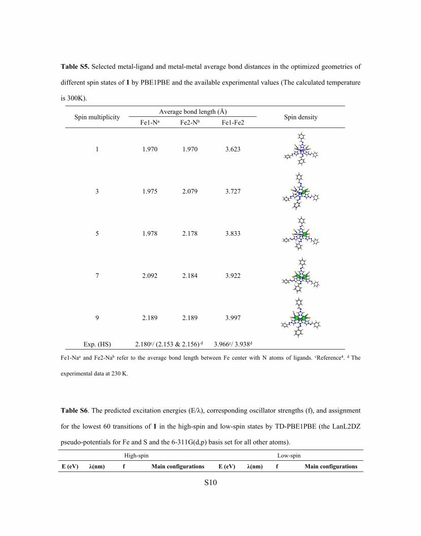
Table S5. Selected metal-ligand and metal-metal average bond distances in the optimized geometries of

different spin states of 1 by PBE1PBE and the available experimental values (The calculated temperature

is 300K).

Average bond length (Å)Spin multiplicity

Fe1-Na Fe2-Nb Fe1-Fe2Spin density

1 1.970 1.970 3.623

3 1.975 2.079 3.727

5 1.978 2.178 3.833

7 2.092 2.184 3.922

9 2.189 2.189 3.997

Exp. (HS) 2.180c/ (2.153 & 2.156) d 3.966c/ 3.938d

Fe1-Naa and Fe2-Nab refer to the average bond length between Fe center with N atoms of ligands. cReference4. d The

experimental data at 230 K.

Table S6. The predicted excitation energies (E/λ), corresponding oscillator strengths (f), and assignment

for the lowest 60 transitions of 1 in the high-spin and low-spin states by TD-PBE1PBE (the LanL2DZ

pseudo-potentials for Fe and S and the 6-311G(d,p) basis set for all other atoms).

High-spin Low-spin

E (eV) λ(nm) f Main configurations E (eV) λ(nm) f Main configurations

S11

0.3183 3894.68 0.0000 2.2085 561.39 0.0000

0.3230 3839.05 0.0001 2.2298 556.02 0.0000

0.4186 2962.01 0.0000 2.2611 548.34 0.0001

0.4258 2911.46 0.0000 2.2731 545.45 0.0000

1.6585 747.56 0.0000 2.2922 540.91 0.0003

1.6722 741.43 0.0000 2.3028 538.40 0.0001

1.8043 687.16 0.0000 3.1307 396.03 0.0190

1.8114 684.45 0.0000 3.1349 395.49 0.0072

2.7874 444.80 0.0000 3.1590 392.47 0.0224H →L+1 (0.31)

H → L (0.27)

2.7920 444.07 0.0000 3.1764 390.32 0.0036

2.7979 439.67 0.0000 3.1959 387.95 0.0026

2.8200 438.90 0.0000 3.2055 386.78 0.0037

2.8249 385.40 0.0006 3.2149 385.65 0.0033

3.2170 384.36 0.0006 3.2236 384.61 0.0303H-2 → L (0.34)

H-1 → L+1 (0.24)

3.2257 380.93 0.0027274B→277B (0.64)

275B→ 277B (0.38)3.2311 383.72 0.0098

3.2548 380.84 0.0021274B→277B (0.48)

275B→ 278B (0.29)3.2390 382.78 0.0065

3.2555 376.41 0.0006 3.2485 381.66 0.0121

3.2939 375.92 0.0004 3.2586 380.49 0.0090

3.2981 372.83 0.0023 274B→278B (0.82) 3.2627 380.00 0.0013

3.3255 370.72 0.0009 3.2774 378.30 0.0135

3.3444 351.93 0.0000 3.2798 378.02 0.0033

3.5230 350.68 0.0000 3.2858 377.33 0.0152

3.5356 345.85 0.0002 3.3027 375.40 0.0137

3.5849 342.26 0.0003 3.3172 373.76 0.0060

3.6225 342.07 0.0002 3.3277 372.58 0.0013

3.6246 341.50 0.0028 273B→276B (0.65) 3.3325 372.05 0.0054

3.6306 339.69 0.0001 3.3426 370.92 0.0037

3.6499 339.39 0.0001 3.3509 370.00 0.0098

3.6531 338.24 0.0006 3.3558 369.47 0.0008

3.6656 338.06 0.0001 3.3628 368.69 0.0106

3.6675 336.53 0.0012 3.3701 367.89 0.0068

3.6842 336.45 0.0001 3.3874 366.01 0.0122

3.6851 336.15 0.0001 3.3961 365.08 0.0051

3.6883 335.56 0.0001 3.4150 363.06 0.0080

3.6949 335.19 0.0002 3.4273 361.76 0.0079

3.6989 335.12 0.0001 3.4302 361.45 0.0053

S12

3.6996 334.87 0.0004 3.4782 356.46 0.0001

3.7025 334.36 0.0001 3.4846 355.81 0.0000

3.7082 333.86 0.0002 3.4961 354.63 0.0000

3.7137 333.06 0.0001 3.5158 352.65 0.0007

3.7225 332.95 0.0001 3.5425 349.99 0.0003

3.7238 332.33 0.0002 3.5508 349.17 0.0032

3.7308 331.73 0.0002 3.5585 348.42 0.0013

3.7375 331.52 0.0006 3.5671 347.58 0.0007

3.7398 330.67 0.0003 3.5689 347.40 0.0008

3.7494 329.69 0.0001 3.5774 346.57 0.0004

3.7606 329.28 0.0001 3.6050 343.93 0.0000

3.7653 328.57 0.0002 3.6131 343.16 0.0003

3.7734 327.93 0.0000 3.6239 342.12 0.0000

3.7808 327.82 0.0008 3.6341 341.17 0.0001

3.7821 327.54 0.0001 3.7887 327.24 0.0001

3.7853 327.15 0.0001 3.8066 325.71 0.0002

3.7899 326.69 0.0002 3.9375 314.88 0.1023 H-8 → L+1 (0.62)

3.7951 325.27 0.0001 3.9502 313.86 0.0270

3.8117 325.03 0.0007 3.9841 311.20 0.0837H-9 → L+1 (0.42)

H-8 → L+3 (0.30)

3.8145 324.48 0.0001 3.9929 310.51 0.0693

3.8210 324.20 0.0004 4.0206 308.37 0.0180

3.8243 324.12 0.0013 4.0305 307.62 0.0557

3.8253 323.57 0.0003 4.0533 305.89 0.0360

3.8317 326.69 0.0002 4.0719 304.48 0.0087

Table S7. Optimized geometries of 1 in the high-spin state.HS

Atom Elem. X coord. Y coord. Z coord.1 C -4.52491300 -1.21561900 0.018845002 H -5.19944400 -0.45073600 -0.331927003 C -3.73255500 -3.10663600 0.708764004 H -3.70374800 -4.13252300 1.04228300

5 C -7.13886600 -2.33783000 0.58429500

6 H -7.05332600 -1.25817700 0.722992007 C -8.48552900 -2.89081400 0.592594008 C -8.73575300 -4.25111700 0.367987009 H -7.90661600 -4.92210000 0.17126400

S13

10 C 10.03541600 -4.72763000 0.3932640011 H 10.22768800 -5.78103500 0.2175180012 C 11.09756200 -3.85728900 0.6394080013 H 12.11451500 -4.23613200 0.6561070014 C 10.85634700 -2.50591600 0.8595120015 H 11.68193200 -1.82799800 1.0491650016 C -9.55456100 -2.02262100 0.8349830017 H -9.35859600 -0.96818400 1.0054720018 C 0.96199200 3.67650900 -1.2274910019 H 1.98074200 4.01706800 -1.3224110020 C -1.20176300 3.62667200 -1.2624580021 H -2.22739900 3.94525600 -1.3640530022 C 0.67156400 6.54748600 -1.4437120023 H 1.50119600 6.20971400 -0.8184930024 C 0.67231800 7.95279300 -1.8198130025 C -0.30608400 8.50309600 -2.6585200026 H -1.09023400 7.86809700 -3.0561630027 C -0.26394700 9.84987300 -2.9761350028 H -1.02172800 10.27507400 -3.6261160029 C 0.75074400 10.66010700 -2.4660270030 H 0.77870000 11.71508300 -2.7197040031 C 1.72682200 10.11927700 -1.6367740032 H 2.51737100 10.74838400 -1.2413130033 C 1.68955600 8.76895700 -1.3151180034 H 2.44807400 8.33812900 -0.6681420035 C 1.08870800 -1.52717600 -2.4457350036 H 2.11934000 -1.73823300 -2.6791850037 C -1.07545800 -1.55116000 -2.4568920038 H -2.09009600 -1.81886300 -2.7061900039 C 0.92534600 -3.84928600 -4.1847510040 H 1.87086100 -3.71598300 -3.6559850041 C 0.89312500 -4.89943300 -5.1922720042 C -0.25322400 -5.17423600 -5.9499170043 H -1.15348500 -4.59101000 -5.7900980044 C -0.22924100 -6.18419000 -6.8964280045 H -1.11765000 -6.39527700 -7.4827160046 C 0.93292200 -6.92889500 -7.09947300

47 H 0.94575000 -7.71792700 -7.84480700

48 C 2.07367300 -6.66107800 -6.3514230049 H 2.97838600 -7.23869000 -6.50956500

S14

50 C 2.05502000 -5.64931200 -5.4002510051 H 2.94276200 -5.43352000 -4.8131590052 C 3.93914300 -2.84486300 0.7519560053 H 3.96432500 -3.89627400 0.9895010054 C 4.57076000 -0.81325900 0.3558600055 H 5.19776600 0.05757000 0.2455260056 C 6.68157600 -3.29926800 1.6264040057 H 5.93794000 -4.00515000 2.0006540058 C 8.07334900 -3.61653000 1.9162260059 C 9.13172400 -2.80624100 1.4842280060 H 8.92120400 -1.91350400 0.9053710061 C 10.43627400 -3.14849500 1.7973940062 H 11.25431600 -2.51918300 1.4621090063 C 10.70173500 -4.29877800 2.5406440064 H 11.72661100 -4.56167600 2.7827220065 C 9.65660300 -5.10863600 2.9699570066 H 9.86148000 -6.00433400 3.5470620067 C 8.34617200 -4.76959200 2.6588460068 H 7.52489400 -5.39749900 2.9918680069 C -1.07354500 0.06777800 2.5475660070 H -2.09478800 -0.03577500 2.8776320071 C 1.09019100 0.09682700 2.5330440072 H 2.11226200 0.04539500 2.8734900073 C -0.82283900 -0.00228500 5.4342540074 H -1.68168500 0.55470100 5.0535920075 C -0.82144200 -0.29946200 6.8583700076 C 0.20496000 -1.03299600 7.4683210077 H 1.02831000 -1.40410200 6.8677850078 C 0.16087900 -1.28008300 8.8296720079 H 0.95622200 -1.84774300 9.3015200080 C -0.90328100 -0.80302900 9.5954180081 H -0.93252200 -1.00127200 10.6621780082 C -1.92616700 -0.07699800 8.9958540083 H -2.75438300 0.29328100 9.5908770084 C -1.88689000 0.17408900 7.6306560085 H -2.68158300 0.74023900 7.1536090086 C -3.80522800 2.25947900 1.8197280087 C -3.89618800 1.05828800 -3.10791700

88 C 3.72572500 1.23501800 -3.17862500

89 C 3.51576300 3.07049900 1.31105700

S15

90 N -3.22356900 -1.11534500 0.1069120091 N -2.71829200 -2.30560600 0.5502810092 N -4.89263800 -2.46494400 0.4013790093 N -6.11651100 -3.09190500 0.4343770094 N 0.58168500 2.46325700 -0.9306030095 N -0.77959800 2.43256400 -0.9443970096 N -0.13856000 4.44600800 -1.4359410097 N -0.26642300 5.76246800 -1.8210580098 N 0.66915600 -0.61140000 -1.6155630099 N -0.69174100 -0.62853000 -1.61798500100 N 0.01164400 -2.15133200 -2.99563200101 N -0.11090300 -3.13931200 -3.94417500102 N 2.87963800 -2.16977200 0.40941500103 N 3.27998200 -0.88496800 0.16611000104 N 5.03492100 -2.02441600 0.73699700105 N 6.36969600 -2.24115100 0.98001400106 N -0.68149200 0.31019400 1.32571500107 N 0.67884200 0.33638600 1.31707200108 N 0.01967600 -0.06446300 3.34407100109 N 0.14444800 -0.37037400 4.68126400110 N -3.22217600 1.84620400 0.88601900111 N -3.22308800 0.95151600 -2.15014100112 N 3.07760700 1.10404000 -2.20639700113 N 3.08777700 2.12655600 0.75628100114 S -4.61504300 2.83430900 3.12827200115 S -4.83594100 1.21168000 -4.44649900116 S 4.63358300 1.41789800 -4.53381500117 S 4.10996100 4.39264400 2.08679900118 Fe -2.03343000 0.67984800 -0.42199800119 Fe 1.96236600 0.77918000 -0.44979900

Table S8. Optimized geometries of 1 in the low-spin state.Atom Elem. X coord. Y coord. Z coord.

1 C 4.18538300 -1.26216600 0.416687002 H 4.88248800 -0.46169000 0.598799003 C 3.31919900 -3.22714800 0.144500004 H 3.24850600 -4.29877600 0.04036100

5 C 6.75974800 -2.57406100 0.20570500

S16

6 H 6.73962400 -1.52067600 -0.080335007 C 8.07467700 -3.18982400 0.314820008 C 8.24425900 -4.53332300 0.675246009 H 7.37412600 -5.14455900 0.8886430010 C 9.51741400 -5.07103100 0.7570230011 H 9.64689700 -6.11185100 1.0354600012 C 10.63312000 -4.27889200 0.4851150013 H 11.62874900 -4.70568600 0.5530500014 C 10.47207400 -2.94476100 0.1291670015 H 11.33903800 -2.32757400 -0.0821090016 C 9.19696500 -2.40104700 0.0435590017 H 9.06290500 -1.35946200 -0.2334150018 C -0.84357700 3.60831000 0.4018490019 H -1.84852000 3.99407900 0.3760480020 C 1.31216000 3.46078700 0.5923840021 H 2.34581400 3.73709200 0.7207620022 C -0.43458400 6.47148800 0.3480470023 H -1.31352700 6.10921300 -0.1889140024 C -0.34471800 7.91041800 0.5448290025 C 0.70843200 8.50467400 1.2529100026 H 1.48751500 7.88152100 1.6783590027 C 0.74610700 9.87980300 1.4079780028 H 1.56158500 10.33890900 1.9572720029 C -0.26191700 10.67568000 0.8632520030 H -0.22800900 11.75307400 0.9905250031 C -1.31034900 10.09215600 0.1610150032 H -2.09515000 10.71041300 -0.2620660033 C -1.35322100 8.71322800 0.0024480034 H -2.16918100 8.24924800 -0.5437410035 C -1.34268700 -0.83451600 2.4461810036 H -2.39782800 -0.91703400 2.6442970037 C 0.81206800 -0.96719900 2.6443790038 H 1.78514800 -1.21357300 3.0355320039 C -1.44701900 -2.71384100 4.6508450040 H -2.30590100 -2.72237500 3.9771780041 C -1.57815800 -3.48617100 5.8771080042 C -0.56491700 -3.53180000 6.8439940043 H 0.35025700 -2.97117600 6.6874420044 C -0.73947500 -4.28673800 7.9912290045 H 0.04509200 -4.31952300 8.74021300

S17

46 C -1.92127300 -5.00152500 8.18827000

47 H -2.05323800 -5.58967000 9.09090900

48 C -2.93048200 -4.96020900 7.2329280049 H -3.85009500 -5.51523400 7.3860670050 C -2.76102800 -4.20394300 6.0806560051 H -3.54487100 -4.16569300 5.3298540052 C -3.70020700 -2.70877500 -0.5084930053 H -3.75347800 -3.78347100 -0.5785500054 C -4.28234500 -0.62535000 -0.4129360055 H -4.88567900 0.26764200 -0.4225030056 C -6.45197400 -3.21214100 -1.3041320057 H -5.71720400 -3.94794200 -1.6361150058 C -7.85176100 -3.55641300 -1.5104930059 C -8.89634500 -2.71187500 -1.1117890060 H -8.66794300 -1.77101600 -0.6229500061 C 10.21027800 -3.08195600 -1.3429750062 H 11.01778400 -2.42603500 -1.0342640063 C 10.49882700 -4.29467100 -1.9691920064 H 11.53107100 -4.57909400 -2.1471220065 C -9.46731500 -5.13890200 -2.3640930066 H -9.69002700 -6.08268700 -2.8508770067 C -8.14743900 -4.77205200 -2.1353320068 H -7.33622000 -5.42620300 -2.4414180069 C 1.28796100 -0.48258200 -2.3458180070 H 2.32294500 -0.69231500 -2.5569620071 C -0.86835000 -0.35222600 -2.5225940072 H -1.86222800 -0.41464700 -2.9335790073 C 1.26065300 -1.11508000 -5.1660350074 H 2.13495100 -0.56458000 -4.8128930075 C 1.34590900 -1.67919300 -6.5041460076 C 0.31065000 -2.43976600 -7.0640310077 H -0.58888000 -2.62784400 -6.4880230078 C 0.44269100 -2.94691000 -8.3453450079 H -0.35977600 -3.53514300 -8.7783120080 C 1.60398100 -2.70563000 -9.0798460081 H 1.70138000 -3.10698100 10.0836330082 C 2.63596600 -1.95445600 -8.5288970083 H 3.53970700 -1.76704600 -9.0992210084 C 2.50859600 -1.44256800 -7.2443680085 H 3.30997400 -0.85431400 -6.80710800

S18

86 C 3.95337400 1.84340400 -1.5813000087 C 3.52471500 1.50815600 2.81677400

88 C -3.69216700 2.01106400 2.16681500

89 C -3.22130700 2.49676300 -2.1379710090 N 2.88839200 -1.13942600 0.2883170091 N 2.33609300 -2.37351100 0.1104470092 N 4.50138500 -2.57940600 0.3222790093 N 5.69615500 -3.24987300 0.4251180094 N -0.50949400 2.34828300 0.3066080095 N 0.83939100 2.25516100 0.4197770096 N 0.28632300 4.34302100 0.5748490097 N 0.48196400 5.68920000 0.7784190098 N -0.79947400 -0.18543200 1.4497300099 N 0.54987200 -0.27334600 1.56906800100 N -0.35062900 -1.35189200 3.21768000101 N -0.37118000 -2.07332400 4.38808800102 N -2.61808400 -2.01534300 -0.29289900103 N -2.98810200 -0.70380900 -0.24161500104 N -4.77577500 -1.87032800 -0.59765700105 N -6.11971700 -2.09705400 -0.77357600106 N 0.81513800 0.00032100 -1.22625900107 N -0.53387900 0.08927600 -1.33865200108 N 0.25036700 -0.71087500 -3.19139400109 N 0.20573600 -1.25402800 -4.45495900110 N 3.16686000 1.38005000 -0.84769200111 N 2.90670500 1.12658700 1.89810900112 N -2.95038800 1.54925400 1.38705200113 N -2.67455400 1.83164600 -1.34432900114 S 5.06037800 2.48926400 -2.62103900115 S 4.38954400 2.04776700 4.11445200116 S -4.73755800 2.66034500 3.26613200117 S -3.98939100 3.43325000 -3.25878400118 Fe 1.85977200 0.55706200 0.35013500119 Fe -1.74037500 0.81691800 0.03909700

S19

5. Additional Figures

Figure S1. ORTEP drawing of the molecular structure of 1, lattice methanol molecules are omitted

for clarity.

0 50 100 150 200 250 3000.0

1.0

2.0

3.0

4.0

5.0

6.0

7.0

T / K

χ MT

/ cm

3 K m

ol-1

T1/2 T1/2

Figure S2. Magnetic properties 1 under applied field of 5000 Oe, sweeping rate: 1 K mol-1.

S20

Figure S3. Solid-state fluorescence spectra of 1 and pnm at room temperature. Excitation: 347 nm

for pnm, 374 nm for 1. Em: emission.

Figure S4. Temperature-dependent fluorescent emission spectra of pnm in the solid states.

S21

(a)

(b)

S22

(c)

(d)

Figure S5. (a) Temperature-dependent fluorescent emission spectra of 1 in the solid states (80-300

K). (b) Temperature-dependent fluorescent emission spectra of 1 in the solid states (80-125 K). The

S23

arrow indicates the trend of emission intensity with increasing temperature. (c) Temperature-

dependent fluorescent emission spectra of 1 in the solid states (130-145 K). The arrow indicates the

trend of emission intensity with increasing temperature. (d) Temperature-dependent fluorescent

emission spectra of 1 in the solid states (150-300 K). The arrow indicates the trend of emission

intensity with increasing temperature.

Figure S6. Experimental spectrum and electronic absorption spectra predicted by TD-PBE1PBE in

methanol solvent for the high-spin state 1. ( Gaussian HFWD is set to 0.333 eV).

S24

Figure S7. Electronic absorption spectra predicted by TD-PBE1PBE in methanol solvent for the low-

spin state of 1. ( Gaussian HFWD is set to 0.333 eV).

S25

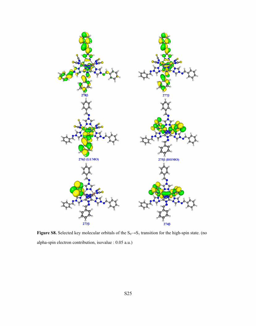
Figure S8. Selected key molecular orbitals of the S0→S1 transition for the high-spin state. (no

alpha-spin electron contribution, isovalue : 0.05 a.u.)

S26

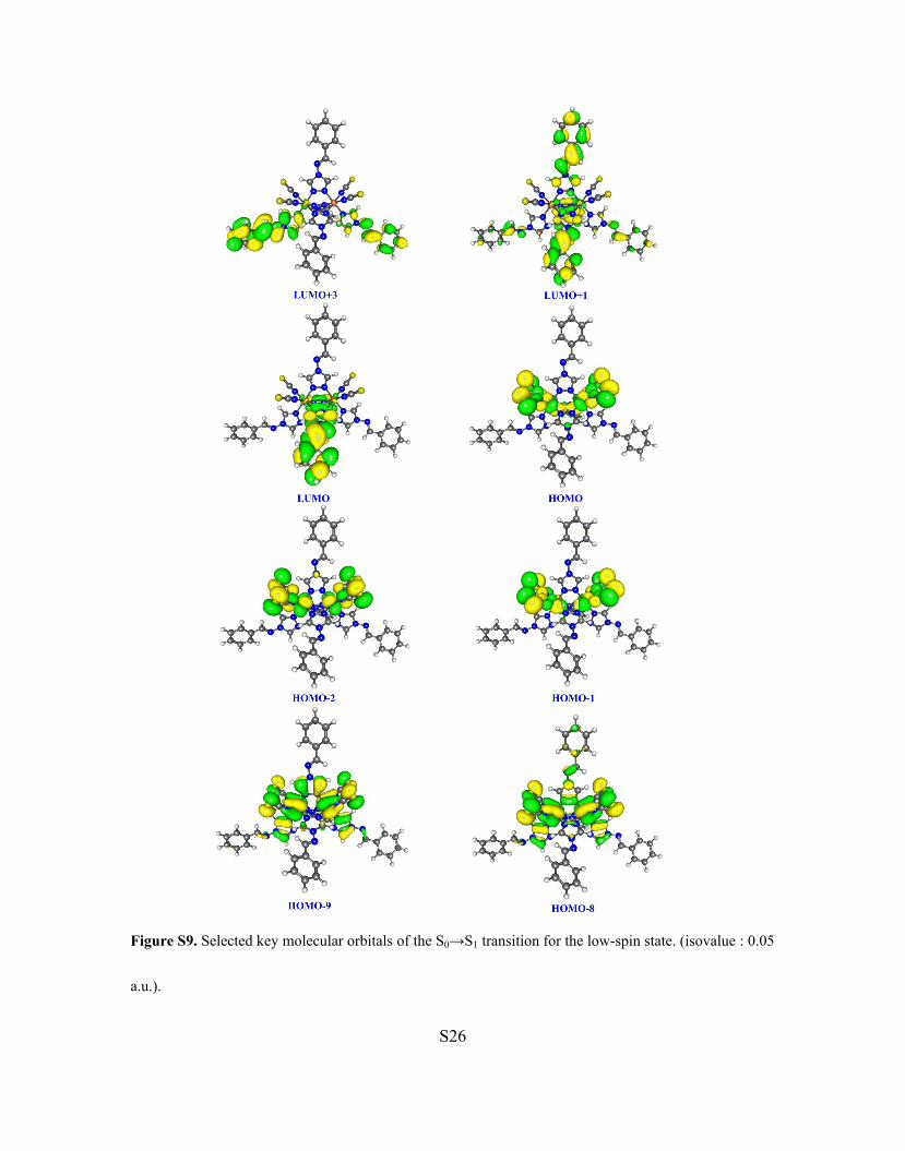
Figure S9. Selected key molecular orbitals of the S0→S1 transition for the low-spin state. (isovalue : 0.05

a.u.).

S27

Figure S10. Electronic absorption spectrum calculated by TD-PBE1PBE in methanol solvent for the

ligand pnm. ( Gaussian HFWD is set to 0.200 eV).

Figure S11. Left: crystal structure of 1 in the LS state obtained by theoretical calculation. Right:

crystal structure of 1 in the HS state obtained by theoretical calculation.

S28

Figure S12. The electronic spin density of 1 in the HS state and in the LS state, respectively, which

were obtained by theoretical calculation.

Figure S13. The normalized diffuse reflectivity spectra (DRS) of pnm.

S29

Figure S14. Normalized excitation spectra and emission spectra of pnm (λex = 347 nm and λem = 466

nm).

S30

6. REFERENCES

(1) Frisch, M. J.; Trucks, G. W.; Schlegel, H. B.; Scuseria, G. E.; Robb, M. A.; Cheeseman, J. R.;

Scalmani, G.; Barone, V.; Mennucci, B.; Petersson, G. A.; Nakatsuji, H.; Caricato, M.; Li, X.; Hratchian,

H. P.; Izmaylov, A. F.; Bloino, J.; Zheng, G.; Sonnenberg, J. L.; Hada, M.; Ehara, M.; Toyota, K.;

Fukuda, R.; Hasegawa, J.; Ishida, M.; Nakajima, T.; Honda, Y.; Kitao, O.; Nakai, H.; Vreven, T.;

Montgomery, J. A., Jr.; Peralta, J. E.; Ogliaro, F.; Bearpark, M.; Heyd, J. J.; Brothers, E.; Kudin, K. N.;

Staroverov, V. N.; Kobayashi, R.; Normand, J.; Raghavachari, K.; Rendell, A.; Burant, J. C.; Iyengar, S.

S.; Tomasi, J.; Cossi, M.; Rega, N.; Millam, J. M.; Klene, M.; Knox, J. E.; Cross, J. B.; Bakken, V.;

Adamo, C.; Jaramillo, J.; Gomperts, R.; Stratmann, R. E.; Yazyev, O.; Austin, A. J.; Cammi, R.; Pomelli,

C.; Ochterski, J. W.; Martin, R. L.; Morokuma, K.; Zakrzewski, V. G.; Voth, G. A.; Salvador, P.;

Dannenberg, J. J.;Dapprich, S.;Daniels,A.D.; Farkas,O.; Foresman, J. B.; Ortiz, J. V.; Cioslowski, J.; Fox,

D. J. Gaussian 09, revision D.01; Gaussian, Inc. : Wallingford, CT, 2009.

(2) Ehlers A W, Böhme M, Dapprich S, Gobbi A, Höllwarth A, Jonas V, Köhler K F, Stegmann R,

Veldkamp A, Frenking G. Chem. Phys. Lett. 1993, 208:111–114

(3) Marenich, A. V.; Cramer, C. J.; Truhlar, D. G. J. Phys. Chem. B 2009, 113, 6378−6396.

(4) Garcia, Y.; Robert, F.; Naik, A. D.; Zhou, G. Y.; Tinant, B.; Robeyns, K.; Michotte, S.; Piraux, L. J.

Am. Chem. Soc. 2011, 133, 15850-15853