improving utilization of associated gas in us tight oil...

Improving utilization of associated gas in US tight oil fields

2


This report was prepared by Carbon Limits AS.

Project title: Improving utilization of associated gas in US tight oil fields

Client: CATF Project leader: Anders Pederstad Project members: Anders Pederstad, Martin Gallardo, Stephanie Saunier Subcontracted companies: Report title: Improving utilization of associated gas in US tight oil fields Report number: Finalized: Revised/Corrected:

April 2015 October 2015

In recent years, tight oil production in the Bakken formation in North Dakota and the Eagle Ford formation in Texas have grown significantly: from 0.2 million barrels a day in 2007 to around 3.1 million barrels a day at the beginning of 2015. Tight oil production now represents a significant share of US oil production. In addition to oil, these wells produce large amounts of natural gas, and in the rush to produce oil, too often this “associated gas” is flared off (burned) instead of being captured and brought to market. Flaring of associated gas in the Bakken and the Eagle Ford basins has dramatically increased, reaching approximately 125 billion cubic feet of gas flared per year by 2013 and remains at similar volumes, enough to provide heat for approximately 1.87 million US homes, until 2015.

This flaring not only wastes energy, it produces air contaminants including toxic volatile organic compounds, smog-forming nitrogen oxides, and particulate matter – most of which is black carbon soot, a very potent climate warmer. And flaring also emits the most prevalent greenhouse gas, carbon dioxide.

The main way to utilize gas is to connect wells to gathering pipelines systems, which convey the gas to a gas processing plant. Gathering systems are in use and being expanded in tight oil production regions in the US. However, pipeline connection is not always feasible, economic, or fast enough to keep up with the rapid pace of oil well development, especially if flaring regulations are lax. In addition, in many locations, flaring at pipeline-connected wells remains a problem because of a lack of compression or other capacity constraints on the gathering system. The technologies that we have identified in this report can minimize flaring at of gas both from wells connected to gas gathering systems and from wells that are isolated from those systems.

In this report, we evaluated nine candidate technologies (beyond gathering pipelines) for capturing and using associated gas. We considered several key factors:

Oil and associated gas production per well declines fast (50-60% in the first year). Ideally, technologies should be able to scale down over time.

On average, 30% of the total well production of associated gas occurs during the first year of production and up to 50% of the total well production of associated gas by the end of the second year. Thus, technologies must be in place as soon as well production begins.

Production volumes have high intraday (x10) variability. Technologies should be able to handle this variability.

Associated gas is generally rich or very rich gas, with substantial amounts of natural gas liquids. Associated gas utilization technologies should work with (and take advantage of) these valuable compounds.

Some wells are isolated and far from both other wells and gas processing infrastructure.

Of the nine alternative technologies that we assessed, the most promising technologies for the utilization of associated gas in the Bakken and the Eagle Ford basins are:

Natural Gas Liquid (NGL) Recovery: separating out heavier hydrocarbons (propane, butane, pentane, etc.), which can easily be transported as liquids, from associated gas. NGL recovery is complementary to other technologies that utilize the remaining gas after NGLs are removed, since this relatively “dry” gas is more suitable for use in compressors and engines and causes fewer problems in gas gathering pipelines.

3


Compressed Natural Gas (CNG) Trucking: compressing associated gas and trucking it to a gas processing plant or other point where it can be transported to market via pipelines.

Gas to Power (to serve local electric demand): generating electrical power with portable units for use at oil and gas production sites.

Gas to Power (grid): generating electrical power for sale to the grid.

These technologies are mature (they have all been deployed commercially at least once in a tight oil development), right-sized and scalable (they can scale up and down depending on the level of gas production at a site), and portable. These technologies are able to handle the conditions found in tight oil formations. In addition to reducing CO2 and other emissions, in many installations, they make money for companies that use them. Based on our research, the other technologies did not meet one or more of our criteria, but they may become mature technologies in the future; flaring regulations may help hasten their commercialization.

Different flaring patterns require different technological approaches. CNG trucking, NGL recovery, and Gas-to-Power (to supply local loads) are best suited for tight oil conditions. Large Gas-to-Power plants for grid power may only be suitable for large multi-well pad developments in areas with small well spacing. Site-by-site variation will also come into play, so decisions about the appropriate gas utilization technology must be based on the specific characteristics of a well site. However, some general findings apply to associated gas from the Bakken and the Eagle Ford:

Bakken Eagle Ford

Characteristic

Very high NGL content (very rich gas)

Greater distance between wells

Harsh winter conditions

High volumes of gas production (high gas-to-oil ratio)

Wells closer together and closer to existing infrastructure

Technology Applicability

Increased profitability of NGL recovery technologies and CNG

Technologies that work well in more remote settings (like gas-to-power for local loads and NGL recovery) will be favorable

Gas-to-power (grid) may be suitable for multi-well pads developments in development “sweet spots”

CNG Trucking most appropriate for wells located relatively close to gas processing plants

Gas-to-power (grid) may be suitable for multi-well pads developments

The technologies identified and described in this study are mature, scalable, portable, and can be economically deployed at tight oil wells. These technologies should be considered during gas capture planning and will give well owners flexibility in identifying beneficial uses for associated gas beyond traditional gas gathering. In short, these technologies make it more feasible to eliminate routine flaring of associated gas. However, this is just one piece of the puzzle, and the flaring problem will continue unless robust regulations limiting routine flaring are put into place in tight oil developments in the US (including Alaska). While there are a variety of technical, geographical, and commercial factors that must be considered, opportunities exist for companies to make a business from the capture and beneficial use of associated gas, making flaring a problem that can be solved.

Special thanks to key technology suppliers and other interviewees that collaborated in the report, among them,

Bakken Express, Hamworthy, GasTechno, LPP Combustion, Blaise Energy, PetroGasSystems, Vortex Tools,

Wellhead Energy Systems, CompactGTL and Wartsila.

Carbon Limits AS accepts no responsibility or liability for the consequences of this document being relied upon by any

other party, or being used for any other purpose, or containing any error or omission which is due to an error or

omission in data supplied to us by other parties. Reproduction is authorized provided the source is acknowledged.

Øvre Vollgate 6

NO-0158 Oslo

Norway

carbonlimits.no

Registration/VAT no.: NO 988 457 930

Carbon Limits is a consulting company with long standing experience in

supporting energy efficiency measures in the petroleum industry. In

particular, our team works in close collaboration with industries,

government, and public bodies to identify and address inefficiencies in the

use of natural gas and through this achieve reductions in greenhouse gas

emissions and other air pollutants.

4


Table of Contents

LIST OF TABLES ....................................................................................................................... 5

LIST OF FIGURES ..................................................................................................................... 5

1. INTRODUCTION .................................................................................................................... 6

CONTEXT AND OBJECTIVES ................................................................................................... 6

BACKGROUND OF THE STUDY ............................................................................................... 7

REASONS FOR FLARING: PIPELINE CONNECTED FLARING VS. ISOLATED WELL FLARING ........... 8

FLARING IN THE BAKKEN AND THE EAGLE FORD ..................................................................... 9

TECHNOLOGY SCREENING .................................................................................................. 11

REPORT STRUCTURE ......................................................................................................... 15

2. FACTORS FOR DETERMINING APPROPRIATE GAS UTILIZATION OPTIONS FOR TIGHT

OIL WELLS .............................................................................................................................. 16

GENERAL TECHNICAL FACTORS .......................................................................................... 16

GENERAL GEOGRAPHIC FACTORS ...................................................................................... 18

GENERAL COMMERCIAL FACTORS ...................................................................................... 18

ENVIRONMENTAL REGULATIONS ......................................................................................... 22

SAFETY REGULATIONS ....................................................................................................... 22

3. EVALUATION OF GAS UTILIZATION TECHNOLOGIES .................................................... 23

COST MODEL USED TO EVALUATE TECHNOLOGIES .............................................................. 23

GAS GATHERING SYSTEMS ................................................................................................. 26

NATURAL GAS LIQUIDS (NGL) RECOVERY ........................................................................... 27

COMPRESSED NATURAL GAS (CNG) TRUCKING,.................................................................. 33

GAS-TO-POWER ................................................................................................................ 36

MINI GAS-TO-LIQUIDS – METHANOL (GTL-MT) ................................................................... 43

GENERAL REMARKS AND COMPARISON ................................................................................ 44

4. TECHNOLOGICAL APPLICABILITY IN THE BAKKEN AND EAGLE FORD ...................... 48

SITE SPECIFIC TECHNICAL FACTORS ................................................................................... 48

SITE SPECIFIC GEOGRAPHICAL FACTORS ............................................................................ 54

SITE SPECIFIC COMMERCIAL FACTORS ............................................................................... 56

5. CASE STUDY: ALASKA ..................................................................................................... 58

OVERVIEW ........................................................................................................................ 58

GAS FLARING REGULATIONS AND MAIN ISSUES REGARDING GAS UTILIZATION OPPORTUNITIES . 59

OPTIONS TO REDUCE FLARING ............................................................................................ 59

TECHNOLOGY APPLICABILITY .............................................................................................. 60

ALASKA SUMMARY ............................................................................................................. 61

6. REFERENCES ..................................................................................................................... 62

5


List of Tables 1. Summary of current flaring regulations in the States of the tight oil plays selected 10 2. Initial Technology Screening 14 3. Gas Gathering Summary 26 4. NGL Constituents 27 5. NGL Summary 29 6. Summary of cost model for NGL recovery (C5+) 31 7. Summary of cost model for NGL recovery (C3+) 32 8. CNG Trucking Summary 33 9. Summary of cost model for CNG trucking 35 10. Gas to Power Summary 38 11. Summary of cost model for gas-to-power (Reciprocating engine) 40 12. Summary of cost model for gas-to-power (Gas turbines) 41 13. Summary of simulation for gas-to-power (Micro turbines) 42 14. Mini Gas-to-liquids (Methanol) Summary 43 15. Expected influence of different variables on project profitability 44 16. Key parameters related to VOC and NOx reduction for selected cases. 46 17. Sensitivity analysis for CNG trucking in a single well with rich associated gas. 46 18. Technical assessment of selected technologies 53 19. Feasibility assessment of selected technologies as a function of geography 56 20. Summary of regulations related to flaring in Alaska 59

List of Figures 1. Estimate of tight oil reserves in major U.S. basins. 2012/2013 data 7 2. Total U.S tight oil production forecast by geologic formation, 2008-2040 (million barrels per day). Forecast in 2013 7 3. Breakdown of Gas Utilization for non-confidential wells in North Dakota in 2013 10 4. Development of associated gas production and gas flared in North Dakota in the last years. Source: NDIC and

rbnenergy.com 10 5. Technologies to reduce associated gas flaring 13 6. Representation of associated gas intraday variations in a tight oil well 17 7. Associated gas production and Technology application strategy: Equipment sized for initial production rates. 19 8. Associated gas production and Technology application strategy: Equipment sized for lifetime average production rates 20 9. Associated Gas production and Technology application strategy: Deployment of three technologies in series with different

production rates. 21 10. Associated Gas production profile for a single well pad 23 11. Associated Gas production profile for a multi well (4) pad 23 12. Hypothetical flaring at a single well with pipeline connection after two years and no other gas utilization technology 24 13. Hypothetical example of flare reduction technology application at a multi well pad 24 14. Range of gas compositions used for the model 25 15. Abatement Cost (left axis) and emission reductions (%) for single and multi-well pads with lean gas composition for

different design of the CNG trucking options 45 16. Net Present Value vs. NOx abatement cost for NGL Recovery C3+ at multi well pad with rich gas. 47 17. Average production profile of a Bakken well based on historical data reported by operators to NDIC until 2014. Profile used

for the economic modeling. 48 18. Expected development of GOR in Bakken, based on the average of historical data reported by operators to NDIC until 2014

48 19. Distribution of associated gas production at different stages of development from wells in the Bakken based on selected

sample 50 20. North Dakota Statewide data on gas utilization for non-confidential wells, data for 2013 51 21. Share of flaring in different months of production per well in the Bakken and Eagle Ford 52 22. Level of flaring and cumulative flaring of all sample wells (different stages of development), sorted by gas produced in Mcf

per day (per well in the Bakken and per lease in Eagle Ford. 53 23. GIS representation of wells in a small area in North Dakota. 54 24. Wellpads (active or under development) in a random location in sweet spots counties in the Bakken and the Eagle Ford.

Both images at the same scale 54 25. Flaring related to distance between wells in Bakken 54 26. North Dakota production wells and tie-ins in 2014 57 27. North Dakota gas plant capacity in 2013 57 28. Shublik/L.Kingak early maturation, peak oil and dry gas windows 58

6


1. Introduction

Context and objectives

Unconventional oil production (also referred to as shale oil or tight oil) is a game-changer in the oil and

gas industry. Upstream exploration and production technologies have helped to unlock oil resources in the

US that were previously uneconomic to recover, leading to rapid growth in domestic petroleum production.

Several basins/formations hold potential for tight oil developments in the US Lower 48 states1: Williston

(Bakken), Niobara, Monterey, Permian (Bone Springs, Wolfberry and Cline), Eagle Ford, Fort Worth, and

Cleveland. The Shublik formation in the North Slope of Alaska2 is also seen as a potentially large play.

While many wells in these basins are drilled primarily to produce petroleum, a significant amount of natural

gas (referred to as associated gas) is produced as well. Thus, this growth in tight oil production has also

led to a significant growth in associated gas production. If the associated gas is captured, it can be sold to

provide additional revenue to oil producers. But, if companies do not proactively create and execute plans

to utilize the associated gas, they must flare (or burn) the gas in order to keep producing oil. Flaring

converts methane and heavier hydrocarbons to carbon dioxide (CO2), black carbon, carbon monoxide,

and various other products of incomplete combustion such as nitrogen oxides. Due to the very rapid ramp-

up in tight oil production, which has outpaced development of infrastructure to handle natural gas, flaring

has markedly increased in the US.

The increase in flaring at the main tight oil plays in the US has raised public concerns over the

environmental harm and wasted resources from this practice. We estimate that approximately 125 billion

cubic feet of gas was flared in the Bakken and the Eagle Ford basins (North Dakota and Texas) in 2013,

which is enough to provide heat for 1.87 million US homes3. Productive utilization of associated gas would

save money, reduce environmental impacts, and make more energy resources available. This report

describes technologies for utilizing associated gas that are relevant for tight oil formations.

Flaring occurs for three main reasons:

Safety Flaring: Flaring may be needed for safety reasons to dispose gases during specific well development and maintenance activities, such as commissioning, start-up/shut-down, and routine or non-routine maintenance. Limited flaring for safety reasons, for short periods of time, may always be necessary, even after a gas gathering pipeline is connected. This type of flaring is not the subject of this report.

Lack of gas utilization capacity – isolated well flaring: If a well begins producing oil and gas with no connection to gas gathering systems or other gas utilization technology, the gas will be flared off.

Lack of gas utilization capacity – pipeline connected well flaring: If a well is connected to gas gathering systems, but those systems cannot handle all of the gas from the well (due to lack of pipeline or compression capacity), some or all of the associated gas from the well will be flared.

Both isolated well flaring and pipeline connected flaring are significant in tight oil basins in the U.S. We

discuss the applicability of technologies for utilizing associated gas examined in this report for both of

these types of flaring.

The most common way of utilizing associated gas, from both tight and conventional oil production, is to

collect gas separated from oil at multiple well pads via a network of gathering pipelines. However, it may

take time to build gas gathering pipeline and other infrastructure for some wells, and often flaring

continues after the pipeline is connected. Therefore, the bulk of this report focuses on other technologies

that can utilize associated gas.

7


Background of the study

1.2.1 Tight oil resources and development4

Tight oil is an industry term that generally refers to medium-to-light grade oil produced from very low

permeability formations, in which oil and gas flow within the rock formation is limited. Production of this

resource requires assistance from advanced drilling and completion processes, such as hydraulic

fracturing and horizontal drilling techniques. Apart from these techniques, tight oil developments follow the

same life cycle as conventional oil developments.

1.2.2 Main tight oil reserves5

Several basins in the US Lower 48 states have potential for tight oil developments: Williston (North Dakota

and Montana); Denver-Julesberg (Eastern Colorado and neighboring states); San Joaquin (the Monterey

Shale formation in California); Permian, Gulf Coast, and Fort Worth in Texas; and Appalachian (where oil

resources are mainly in Ohio)6. The Shublik formation in the Alaskan North Slope is also a potentially large

play7 (Figure 1).

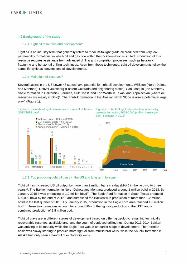
Figure 1: Estimate of tight oil reserves in major U.S. basins. 2012/2013 data8

Figure 2: Total U.S tight oil production forecast by geologic formation, 2008-2040 (million barrels per day). Forecast in 20139

1.2.3 Top producing tight oil plays in the US and long term forecast

Tight oil has increased US oil output by more than 2 million barrels a day (bbl/d) in the last two to three

years10. The Bakken formation in North Dakota and Montana produced around 1 million bbl/d in 2013. By

January 2015 it was producing at 1.2 million bbl/d11. The Eagle Ford formation in South Texas produced

400,000 bbl/d by the end of 201212 and surpassed the Bakken with production of more than 1.2 million

bbl/d in the last quarter of 2013. By January 2015, production in the Eagle Ford area reached 1.6 million

bpd13. These two formations account for around 80% of the tight oil production in the US14 and a

combined production of 2.8 million bpd.

Tight oil plays are in different stages of development based on differing geology, remaining technically

recoverable reserves, available land, and the count of deployed drilling rigs. During 2013-2014 Bakken

was arriving at its maturity while the Eagle Ford was at an earlier stage of development. The Permian

basin was slowly starting to produce more tight oil from multilateral wells, while the Shublik formation in

Alaska had only seen a handful of exploratory wells.

7413

6742

527

1732 3

026

1409

40 1417

35

940

939

9

O I L [ M M B O E ] G A S [ B C F G ] N G L S [ M M B N G L ]

Williston Basin / Bakken (2013)Gulf Coast / Eagle Ford (2012)Alaska - North Slope (2012)Appalachian basin - Marcellus (2012)

8


The EIA expects US tight oil production to grow to a peak of approximately 5 million bbl/d between 2016

and 202515 with the largest production from the Eagle Ford and the Bakken (See Figure 2)16. However,

tight oil wells are characterized by fast decline rates—between 50% and 70% during the first year of

production17. These decline rates and the drilling pace limit production growth. Peak production from the

Bakken and the Eagle Ford could occur as early as 2015 - 201718.

1.2.4 Associated Gas Production and Utilization19

As hydrocarbon fluids are brought to the surface at a tight oil well pad, associated gas is separated from

the oil, water, and other elements. Compared to oil, associated gas has low energy density and value, and

it is challenging to store and transport. Further, compared to processed natural gas distributed to homes

and industries, associated gas at well pads typically contains significant amounts of natural gas liquids

(NGLs).

Based on the above data for the Bakken and the Eagle Ford, we estimate that between 3-4 Bcf per day of

associated gas were produced from tight oil in the US at the end of 2013 and that, under business as

usual conditions, associated gas production will increase in the next few years as tight oil output

increases.

As a general rule of thumb, about half of the lifetime well production of associated gas occurs during the

first two years of production. In order to capture as much of the associated gas produced in the first year

as possible, data from drilling/completion and initial well testing is used to assess expected associated gas

production. Using the expected gas composition, gas decline curve, and other geographical and economic

factors, well owners can find the most appropriate gas utilization option.

Reasons for Flaring: Pipeline Connected Flaring vs. Isolated Well Flaring

It is important to differentiate the reasons for flaring between fields already connected and those not yet

connected to gas infrastructure.

1.3.1 Pipeline connected well flaring

A significant share of the flaring related to tight oil production occurs at well pads that are already

connected via gas gathering networks to centralized, downstream infrastructure20. Aside from safety

flaring, which is not considered in this report, pipeline connected flaring can be related to, among other

things:

Pressure imbalance in the line: Increased infield drilling, especially horizontal drilling, and the fast decline rates of tight oil, has brought many new wells on stream at high rates of production and pressure, relative to the older wells in the same reservoir. Gas from these new wells takes up gas gathering systems capacity and increases the pressure in the gathering system. If compressors are not added to the system, lower pressure gas from older wells cannot send gas into the gathering system, which may result in flaring.

Natural Gas Liquids (NGL) pooling: The rich nature of the associated gas from tight oil makes extraction and processing of NGLs an attractive option. On the other hand, high liquid content can also create some challenges, depending on how the gas is handled and used. NGLs can condense out of the gas stream due to pressure / temperature conditions and pool in the pipes, clogging them. Variations in topography (valleys and hills) will also increase NGL pooling. Liquid condensation can reduce the effective capacity of gas gathering systems and block pipelines in low spots if provision is not made for removing NGLs.

9


Temporarily limitations on gas processing capacity: Gas processing plants may be unavailable during short-term gas oversupplies, operation and maintenance routines, power outages, or expansion of facilities. If oil production is allowed to continue, large-scale flaring (millions of cubic feet of gas and thousands of gallons of NGLs flared per day) may go on for some time.

Long-term limited gas gathering capacity: If the development of gas gathering infrastructure lags behind as drilling moves forward, pipeline capacity may be too low to handle associated gas production.

1.3.2 Isolated well flaring or “Last mile problem”

In the best case, the well will be connected to gas gathering infrastructure before well completion. This is

often made possible by signing an agreement with a midstream company. Such an agreement would

provide revenue stream to the well operator and reduce flaring emissions without significant investment by

the operator. Instead, the midstream company uses its capital and expertise to build the pipeline, and

generate profit by selling the gas. In our interviews with industry sources, we found that some midstream

companies prefer not to tie-in new wells in the first few months of production to the gas gathering systems

due to operational problems caused by the high pressure and volume from these new wells. However, it is

rare for a well operator to build gathering pipelines in the absence of such a midstream agreement. Even

when there is gas processing plant or interstate pipeline nearby, there may still significant cost for the well

operator to tie-in to the pipeline. Deployment of pipelines can be costly – large diameter pipeline costs

between 30,000 and 100,000 USD/inch-mile and increasing rapidly 21– and may take several months to

one year before approval is given and construction finished.

Thus, some isolated wells or well pads are unable tie-in to gas processing plants or existing infrastructure

due to very high costs and extended timelines of gas gathering system deployments. Some wells in

remote areas will flare for 1 or 2 years until a pipeline is in place, and some flare indefinitely over the full

productive life of the well.

Flaring in the Bakken and the Eagle Ford

In North Dakota flaring volumes have increased substantially over the last few years, following the

remarkable increase in the rate of tight oil production. The portion of gas flared has increased from around

5% in 2005 to over 30% by 2010.22. In the Bakken the share of flaring from isolated well and pipeline

connected flaring is quite similar. In 2013, associated gas flaring was around 32%, of which 14% was from

isolated wells, while the remaining 18% was from pipeline connected wells (as shown in Figure 3).

Between November 2013 and May 2014 the amount of pipeline connected flaring rose significantly

because an important gas processing plant was taken off-line for expansion23. Starting in the second half

of 2014, the percent of gas flared in North Dakota has dropped, but the total volume of gas flared has

stayed constant or increased as the growth in production outpaced the progress in capturing gas (as

shown in Figure 4).

In comparison, flaring as a percent of total gas volumes in the Eagle Ford is approximately 10%, which is

partially due to the proximity of oil wells to gas infrastructure in the Eagle Ford. The Eagle Ford contains

both oil wells and wells that are primarily drilled for natural gas, so flaring as a percent of total associated

gas produced at oil wells is likely much higher (combined to the flaring rate for oil and gas wells

combined).

Combining these flaring percentages with the current production rates, a conservative estimate of flared

volumes from the Bakken and the Eagle Ford would be at least 0.35 Bcf per day (over 125 Bcf per year) in

2013. Recovering that gas could meet the annual needs of approximately 1.87 million US homes24.

10


Figure 3: Breakdown of Gas Utilization for non-confidential wells in North Dakota in 201325

Figure 4: Development of associated gas production and gas flared in North Dakota in the last years. Source: NDIC and rbnenergy.com

A number of factors related to well licensing, leasing, and permitting have contributed to flaring in the

Bakken and the Eagle Ford26. Well operators often acquire the right to exploit subsurface oil deposits

through a mineral lease, rather than purchasing the mineral rights. Such a lease, whether obtained from a

public or private landowner, may obligate the oil company to operate the well and produce the oil if a

sufficient quantity is found, with strong incentives for rapid production. Such lease stipulations often

hasten well development and oil production. In the absence of regulations that require companies to

create gas utilization plans in advance, rapid oil well development will lead to increased flaring.

Drilling and completion typically last around a month, and flaring may be substantial during that time

(especially during completion). Once in operation, little additional investment is required for continued oil

production at the well, and oil production from the first year can be very lucrative. Limiting the rate of

extraction during this first year to avoid excessive flaring may not be considered economical by the

operator, and in some cases it is be constrained by contractual agreements. Nevertheless, the rate of oil

production will have a direct impact on flaring if gas infrastructure of sufficient capacity is not in place from

day one.

In addition, many well operators have small leases scattered over a large area. Such a scenario may

make it more challenging for operators to achieve economies of scale to economically develop certain gas

utilization technologies. This trend has begun to abate as the most desirable acreage in the Bakken and

the Eagle Ford have largely already been leased, and producers have sought to achieve economies-of-

scale by buying, selling, and trading assets to increase the size of their continuous lease acreage27. This

tendency for unitization of activities within an area by a single operator could help reduce flaring of

associated, as coordination among different, neighboring well operators to develop gas gathering

infrastructure increases.

Strong regulations will provide incentives for companies to develop gas utilization plans in advance and

can impose penalties for companies that exceed flaring thresholds. Historical oil regions, like Texas,

regulate emissions from flaring either by promoting gas distribution and marketing28 or by requiring gas

reinjection. Texas provides a number of exemptions, and only strictly constrains long term flaring after 6

months from first production from significant sources of flaring (over 50 mscf per day). Until 2014, North

Dakota had fewer regulations to limit flaring (see Table 1).

Table 1: Summary of current flaring regulations in the States of the tight oil plays selected

Texas29 North Dakota30

11


Flaring after completion Allowed for 10 days Allowed for 90 days

Isolated well permit 45 days Operator must meet gas capture targets (“74% of the gas

by October 1, 2014; 77% by January 1, 2015; 85% by

January 1, 2016; and 90% by October 1, 2020”);

percentages only apply to gas produced after 90 days. If

gas capture target is not met, the operator must curtail oil

production at the site (“If such gas capture percentage is

not attained at maximum efficient rate, the well(s) shall be

restricted to 200 barrels of oil per day if at least 60% of the

monthly volume of associated gas produced from the well is

captured, otherwise oil production from such wells shall not

exceed 100 barrels of oil per day.”)

Additional flaring permita 45 days

Maximum permitted

period

First 180 days

After, sources > 50 Mscfd

Long term flaring

allowance

Rare, only if well/compressor need to

be repaired

Pipeline-Connected

flaring allowed under the

following circumstances

Insufficient capacity, gas plant

shutdowns; repairing a compressor or

gas line or well; or other maintenance

Overall Strict on flaring, lax on exemptions New regulations may improve the situation, but still allow 3 months of flaring before restrictions are imposed.

Technology screening

To improve the understanding of why associated gas is being flared and what additional measures can be

taken to minimize flaring related to US tight oil developments, Clean Air Task Force (CATF) commissioned

Carbon Limits to study:

The availability and suitability of alternative technical solutions that can be implemented quickly and at various scales to increase associated gas utilization at single and multi-well pads, and thus reduce flaring of associated gas.

The applicability of these technologies to utilize associated gas in the Bakken and the Eagle Ford basins.

In this report, we present several alternative technologies for utilizing associated gas, each of which is

mature, commercialized, demonstrated in tight oil formations, and able to be scaled sufficiently to utilize

meaningful quantities of associated gas. As described above, flaring from both isolated and pipeline-

connected tight oil wells is significant. Thus, we assessed on-site solutions that can help minimize flaring

in either situation. To avoid flaring, either sufficient infrastructure must be in place to efficiently move the

associated gas into a centralized gas supply system, or the operator must use an on-site gas utilization

technology. These technologies should be considered as part of the decision process before oil

production commences. In a screening process, we examined nine facilities to determine whether they

are presently feasible to utilize associated gas from tight oil formations in order to reduce flaring:

1) Ammonia production: Ammonia is a commodity chemical that can be produced by combining high-pressure hydrogen and nitrogen to produce ammonia. Nitrogen is obtained from air, which is deoxygenated by the combustion of natural gas. Hydrogen can be obtained via steam reforming, which converts methane into a mixture of carbon monoxide and hydrogen.

2) Compressed natural gas (CNG) trucking: Compressing lean associated gas at wellpads and trucking it to consumers, gas gathering systems, etc.

3) Natural gas liquids (NGL) recovery: Separating NGLs (heavier hydrocarbon which can be stored as liquids under pressure) from raw associated gas at wellpads, so that NGLs can be trucked to market. The residual lean associated gas can be utilized further with other technologies, and NGL recovery may make the gas more suitable for those technologies. If not utilized, the residual associated gas is flared, producing less CO2 and other pollutants than if the entire gas stream was flared.

a Document infrastructure plans

12


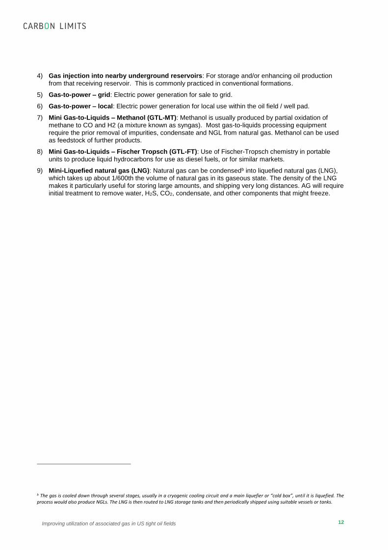
4) Gas injection into nearby underground reservoirs: For storage and/or enhancing oil production from that receiving reservoir. This is commonly practiced in conventional formations.

5) Gas-to-power – grid: Electric power generation for sale to grid.

6) Gas-to-power – local: Electric power generation for local use within the oil field / well pad.

7) Mini Gas-to-Liquids – Methanol (GTL-MT): Methanol is usually produced by partial oxidation of methane to CO and H2 (a mixture known as syngas). Most gas-to-liquids processing equipment require the prior removal of impurities, condensate and NGL from natural gas. Methanol can be used as feedstock of further products.

8) Mini Gas-to-Liquids – Fischer Tropsch (GTL-FT): Use of Fischer-Tropsch chemistry in portable units to produce liquid hydrocarbons for use as diesel fuels, or for similar markets.

9) Mini-Liquefied natural gas (LNG): Natural gas can be condensedb into liquefied natural gas (LNG), which takes up about 1/600th the volume of natural gas in its gaseous state. The density of the LNG makes it particularly useful for storing large amounts, and shipping very long distances. AG will require initial treatment to remove water, H2S, CO2, condensate, and other components that might freeze.

b The gas is cooled down through several stages, usually in a cryogenic cooling circuit and a main liquefier or “cold box”, until it is liquefied. The process would also produce NGLs. The LNG is then routed to LNG storage tanks and then periodically shipped using suitable vessels or tanks.

13


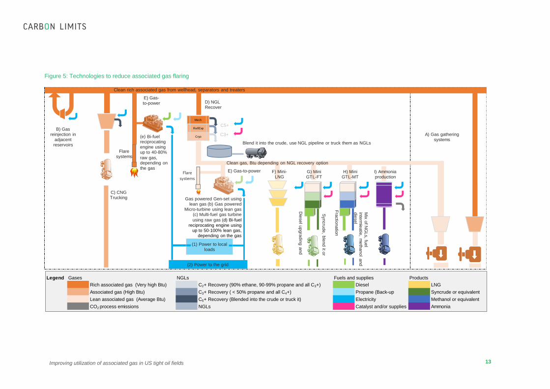
Figure 5: Technologies to reduce associated gas flaring

B) Gas reinjection in

adjacent reservoirs

D) NGL Recover

Mech

Ref/Exp

Cryo

C) CNG Trucking

(e) Bi-fuel reciprocating engine using up to 40-80%

raw gas, depending on the gas

Gas powered Gen-set using lean gas (b) Gas powered

Micro-turbine using lean gas (c) Multi-fuel gas turbine

using raw gas (d) Bi-fuel reciprocating engine using

up to 50-100% lean gas, depending on the gas

(1) Power to localloads

(2) Power to the grid

Flare systems

Flare

systems

Blend it into the crude, use NGL pipeline or truck them as NGLs

Clean rich associated gas from wellhead, separators and treaters

Clean gas, Btu depending on NGL recovery option

F) Mini-LNG

Die

sel u

pgra

din

g a

nd

Syn

cru

de

, ble

nd

it or

Fra

ctio

na

tion

Mix

of N

GLs, fu

el

inte

rmie

atie

, meth

ano

l an

d

die

se

l

G) Mini GTL-FT

E) Gas-to-power

E) Gas-to-power

H) MiniGTL-MT

I) Ammoniaproduction

A) Gas gathering systems

C5+

C3+

Legend Gases NGLs Fuels and supplies Products

Rich associated gas (Very high Btu) C2+ Recovery (90% ethane, 90-99% propane and all C3+) Diesel LNG

Associated gas (High Btu) C3+ Recovery ( < 50% propane and all C4+) Propane (Back-up Syncrude or equivalent

Lean associated gas (Average Btu) C5+ Recovery (Blended into the crude or truck it) Electricity Methanol or equivalent

CO2 process emissions NGLs Catalyst and/or supplies Ammonia

Clean rich associated gas from wellhead, separators and treaters

14


Based on the characteristics of the tight oil formations that we will describe throughout the report, we

considered whether these technologies meet the following criteria:

Mature: The technology is a common in natural gas applications and has been deployed commercially more than once in tight oil developments. Also, the procurement process should allow for delivery within weeks or months.

Right-sized and Scalable: Technology should be able to scale down to the size of the developments (100 – 1,000 Mscfd per well) without becoming prohibitively expensive. Scaling up should be modular and a rapid process for an operator. Different contractual options, like leasing or renting, are a plus but not required.

Portable: The technology should be portable able to be delivered within a week (one day is a plus), during the first year of operations, where most of the value can be captured. After the first year, the equipment can be dismantled or scaled down once a pipeline is in place.

We found that four technologies are suitable for large-scale use to reduce flaring, based on these criteria.

Three of these are proven for utilization of associated gas from tight oil wells. As Table 2 shows, we

further broke out these four technologies into two categories: “Ready for tight oil” and “Ready at larger

scales”. Another category—“On the radar”—includes one additional technology that is ready to

commercialize but not yet commercially proven at tight oil wells.

Table 2: Initial Technology Screening

Ready for tight oil: Proven on tight oil. Scalable and portable technologies. Supply chain ready if

widespread

Economic

model

CNG Trucking - Proven, operating currently at 5 or more well sites Included

NGL Recovery - Proven, current operations at several sites, mainly with relatively simple processes

(minimizing cost, but also limiting NGL recovery) Included

Gas-to-power -

Local loads - Proven, current operations at several sites, including drilling and completion operations Included

Ready at larger scales: Feasible, ready for large developments Economic

model

Gas-to-power –

Grid Connected

- Proven for lean associated gas in tight oil developments

- Scale is too big for average well, completely uneconomic to scale down to single wells due to

the cost of certain equipment. Only feasible when at least 1,000 Mscf associated gas per day is

available; feasibility also depends on distance to electric grid infrastructure

Not

included

On the radar: Ready to commercialize but not commercially proven on tight oil. Scalable and portable

technologies. Supply challenges may occur with widespread use.

Economic

model

Mini GTL-MT - Pilot running on tight oil fields with promising results. Waiting for first commercial deployment Not

included

15


Appendix 2 briefly discusses the remaining four technologies. While they did not meet one or more of our

criteria, they may become mature and commercialized in the future.

For each of the “Ready for tight oil” technologies, we analyzed the economic and environmental impact of

each technology described in this chapter using a simple and straightforward cost model. In this model,

we have made reasonable assumptions about associated gas production and composition in tight oil

formations in the US, and we have used cost data from industry sources to assess the economics of

various project scenarios. The model is meant to be illustrative of the numerous options available for well

operators to reduce flaring. (A more detailed description of the cost model can be found in Appendix 4). As

described in Chapter 2, a number of technical, geographic, and commercial factors influence the

economics of a given technology.

Report structure

In Chapter 1, we provide an overview of problem and describe the scope of our study. In Chapter 2, we

consider technical, geographical, and commercial factors that affect flaring and the economic viability of

flaring alternative technologies. In Chapter 3, we assess information on technologies from a review of

previous studies, technical documents, and interviews with suppliers. We have assessed the advantages

and disadvantages of the five technologies that passed our initial screening. We also present the results of

a cost analysis for several of the technologies. In Chapter 4, we summarize the role that these

technologies can play to improve gas utilization in two tight oil formations in the US: the Eagle Ford in

Texas and the Bakken in North Dakota. In Chapter 5, we summarize the role that these technologies can

play to improve gas utilization in a tight oil basin with a large resource potential which is quite distant from

natural gas consumers: the Shublik on Alaska’s North Slope.

Appendix 1: Summary charts with details on five technologies that passed initial screening.

Appendix 2: A description of technologies that did not pass initial screening.

Appendix 3: Case studies on technologies.

Appendix 4: Description of the economic cost model.

16


2. Factors for determining appropriate gas utilization options for tight

oil wells

In this chapter, we discuss factors that impact the utilization of associated gas from tight oil formations:

Technical: Tight oil formations produce associated gas with highly variable composition, flow rates, and pressures; utilization options must handle this variation. Complex utilization systems complicate well operations with new equipment and processes.

Geographical: Expected production of associated gas from tight oil wells may not justify the cost of connecting wells to distant gathering systems or electrical grids. However, other utilization options can be feasible at greater distances to markets.

Commercial: Feasibility of utilization options varies with different reserves, economic conditions, and corporate characteristics, so no single approach will serve all tight oil wells adequately. Commercial factors may hinder getting gas or electricity to markets.

In addition, a variety of legal and regulatory factors can either hinder or promote the deployment of gas

utilization technologies.

General Technical Factors

2.1.1 Gas Quality

The composition of gas and the presence of natural gas liquids (NGLs, i.e. heavy hydrocarbons, including

ethane, propane, butanes, and other heavier compounds) vary from well to well and at the same well over

time. Compared to processed natural gas distributed to homes and industries, associated gas produced at

tight oil well pads typically contains high levels of NGLs. These components are valuable if they are

extracted from the gas stream and marketed separately, but they may represent a technical challenge for

gas utilization when they are not removed.

Traditional gas processing has better economic returns when the gas stream contains a larger proportion

of heavier hydrocarbons (“rich gas”), while other utilization options, such as electricity generation, typically

require gas with these heavier hydrocarbons largely removed (“lean gas”).

Associated gas composition tends to vary over time as a result of multiple factors, including reservoir

behavior, well depletion, changes in recovery techniques, and operating conditions. Future changes in

associated gas compositions are difficult to predict accurately, making it more challenging to design

facilities for associated gas than for dry natural gas. Different associated gas streams can have large

variations in gas composition and impurities, and thus may require different levels of treatment. The

variation in composition also means that different associated gas streams will provide different product

yields and thus different economic values, even when the same technological solutions are used.

In addition to composition, varying levels of gas pressure (resulting from reservoir conditions and

production facilities design) can cause problems in gas gathering systems. An associated gas stream will

always be more attractive when it is at elevated pressures, due to reduced costs required for treatment

and compression. However, infield drilling and fast decline rates have allowed these high pressure new

wells to come on stream at high rates relative to older wells, and new wells both take up gas gathering

capacity and can knock low-pressure wells off, leading to pipeline connected well flaring.

17


2.1.2 Time-Lapse Distribution

The amount of associated gas produced at a well will decline over time; up to half the total well production

of associated gas usually occurs during the first two years of production. In order to capture as much this

first year production as possible, initial well testing and data compilation must be collected prior to well

development, as all technologies need a preliminary assessment of the amount of gas that can be

expected. Once oil and gas operators have access to the expected gas composition, gas decline curve,

and other geographical and economic factors, they can perform a techno-economic assessment to find

the most appropriate gas utilization option. Given the intrinsic uncertainty associated to well performance,

the assessment could cover several scenario and focus on flexible options.

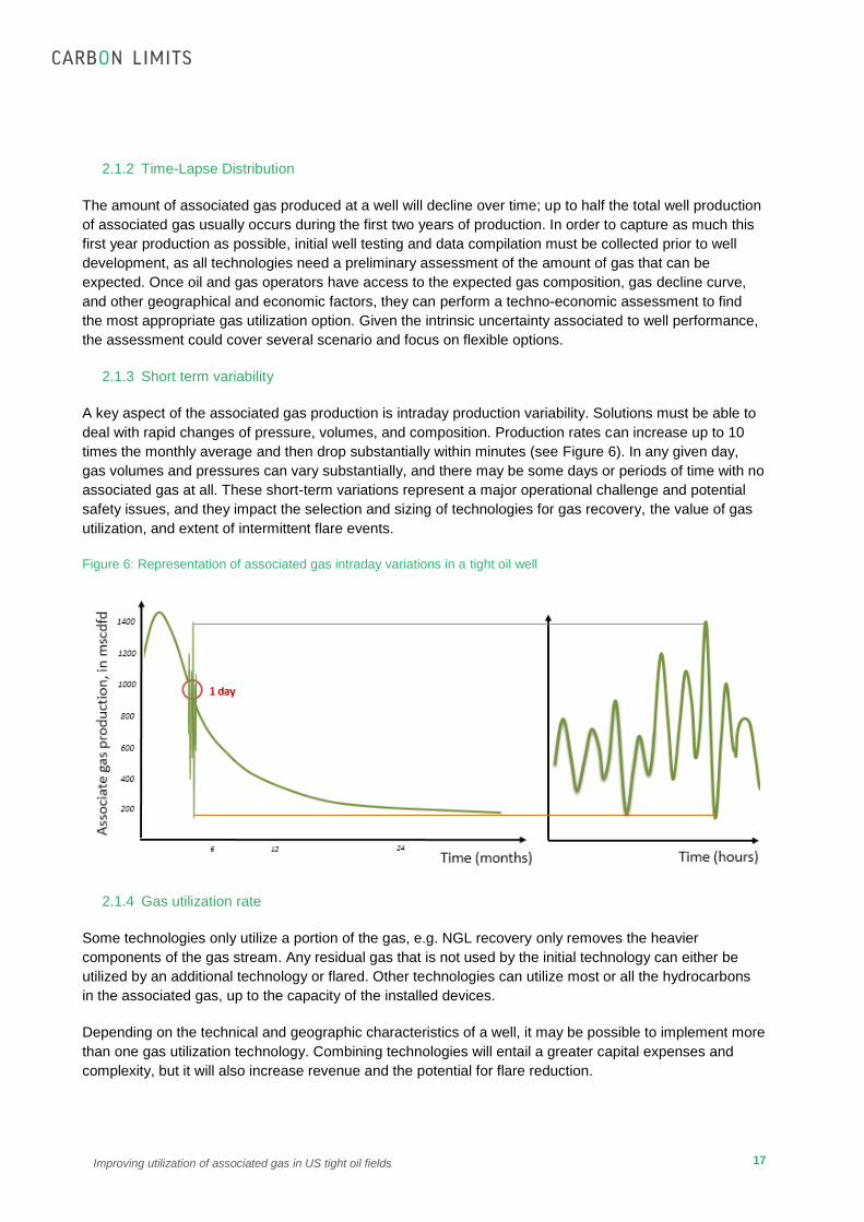
2.1.3 Short term variability

A key aspect of the associated gas production is intraday production variability. Solutions must be able to

deal with rapid changes of pressure, volumes, and composition. Production rates can increase up to 10

times the monthly average and then drop substantially within minutes (see Figure 6). In any given day,

gas volumes and pressures can vary substantially, and there may be some days or periods of time with no

associated gas at all. These short-term variations represent a major operational challenge and potential

safety issues, and they impact the selection and sizing of technologies for gas recovery, the value of gas

utilization, and extent of intermittent flare events.

Figure 6: Representation of associated gas intraday variations in a tight oil well

2.1.4 Gas utilization rate

Some technologies only utilize a portion of the gas, e.g. NGL recovery only removes the heavier

components of the gas stream. Any residual gas that is not used by the initial technology can either be

utilized by an additional technology or flared. Other technologies can utilize most or all the hydrocarbons

in the associated gas, up to the capacity of the installed devices.

Depending on the technical and geographic characteristics of a well, it may be possible to implement more

than one gas utilization technology. Combining technologies will entail a greater capital expenses and

complexity, but it will also increase revenue and the potential for flare reduction.

18


General Geographic Factors

The applicability of gas utilization technologies depends on geography in two ways: (i) the distance from

the well to gas gathering/power networks or infrastructure, and (ii) the concentration of nearby wells. The

closer a well is to gathering/power networks, the more options the operator will have for associated gas

recovery. But, options are still available at remote well sites. Likewise, if a well is located near other well

pads, it may be able to share resources to get gas to market. An isolated well may have fewer options.

2.2.1 Distance

In general, well pads that are located near existing infrastructure and markets will have more gas

utilization options. For wells that are less than 5 miles from existing infrastructure, connection to traditional

gas gathering pipelines may be the most profitable option. If other factors prevent or delay access to the

gas gathering system, several other gas utilization technologies will still be profitable. At medium

distances, some of these technologies will be infeasible or uneconomical. Even remote well pads will have

options to reduce flaring.

2.2.2 Concentration

A higher well concentration enables economies of scale. Moreover, when several associated gas streams

are combined, the overall associated gas stream is more stable. Multi-well pads or several pads together

would also improve the attractiveness of gas utilization options and make these solutions viable even

when further from markets or gas gathering / power networks.

Isolated well sites could also benefit from sharing utility and transportation infrastructure, which may bring

savings and enable economies of scale and collaboration between larger players to develop gas gathering

systems and other gas utilization projects. This requires a high level of planning and cooperation between

the various stakeholders, which often include governments, oil companies, and other investors. Such

coordination would also improve future field design and tight oil operations for associated gas utilization

and flare reduction. If this type of field value optimization were to be turned into a separate business

(perhaps through regulatory or tax benefit encouragement to initiate it), the technology suppliers could

optimize the conditions and field design/operation.

General Commercial Factors

Each well site has a different level of associated gas production and each gas utilization technology

comes with different levels of capital investment, operational expenses, expected revenues, and risk.

Regional market variations can also change capital and operating cost of utilization options, and marketing

and value of the products.

2.3.1 Equipment scaling

Based on the decline pattern of associated gas production at wells, there are three main equipment

scaling options (See Figure 7, Figure 8 and Figure 9).

19


Equipment sized for initial production rates.

As we discussed above, a large amount of associated gas is produced during the initial stages of well production. Thus, operators can select equipment that is large enough to capture this initial surge of gas. Installing capacity sized to initial production rates does not necessarily guarantee capturing all gas during the first months of peak production. This strategy may also leave a very large amount of spare capacity after the peak production period, due to the rapid decline profile. This strategy is not appropriate for technologies that can only operate with a narrow range of gas feed rates. However, if the technology is able to handle these variations, this approach guarantees a substantial gas recovery through the lifetime of the well.

If gas flow from multiple wells (from a single well pad and/or from closely-spaced pads) can be pooled, the relative flow rate variation of the combined flow will be significantly less than the flow from a single well, mitigating this issue considerably, particularly if the wells have staggered initial production dates.

Figure 7: Associated gas production and Technology application strategy: Equipment sized for initial production rates.

20


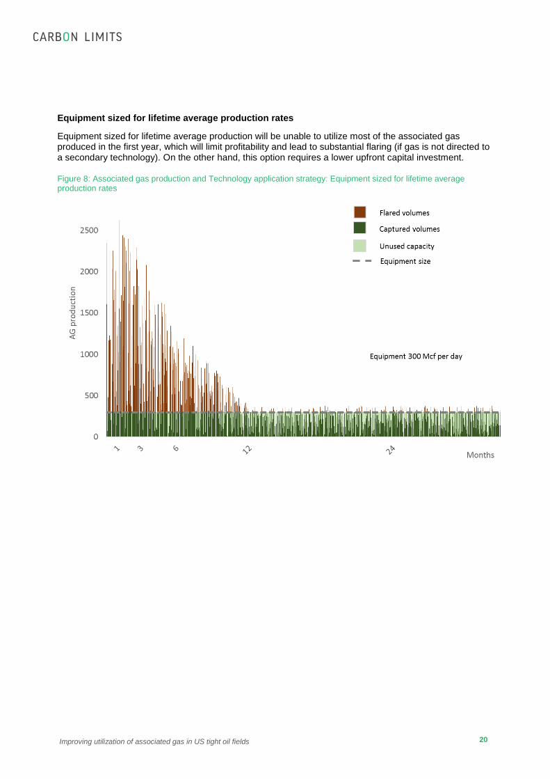
Equipment sized for lifetime average production rates

Equipment sized for lifetime average production will be unable to utilize most of the associated gas produced in the first year, which will limit profitability and lead to substantial flaring (if gas is not directed to a secondary technology). On the other hand, this option requires a lower upfront capital investment.

Figure 8: Associated gas production and Technology application strategy: Equipment sized for lifetime average production rates

21


Leasing, renting, or scaling in series

For some of the gas utilization technologies, operators have the option of leasing equipment, rather than purchasing it outright. This strategy will allow operators to avoid upfront capital costs associated with purchasing equipment, and it will allow them to match equipment size to expected associated gas production volumes at different stages of well production. Also, some of the technologies are portable, so operators can move larger equipment from older wells to new wells. Thus, this strategy can help to optimize the total amount of gas recovered. Flaring may still be required for short periods of time as equipment is switched out. H

Figure 9: Associated Gas production and Technology application strategy: Deployment of three technologies in series with different production rates.

2.3.2 Contracts

The flexibility and profitability of the gas utilization technologies depends on the nature of the contractual

agreements made between the well operator and the midstream gas company. Several different business

models are available—fee for services, monetization of products, etc.—so these contracts can be quite

complex.

It also depends on where the operating company wants to set their upstream/downstream boundaries and

the contractual aspects of each business deal. Larger well operators seem more reluctant to connect

existing wells by tying to gathering lines when they can earn a higher return on investment by drilling new

wells.

We were not able to access to any examples if agreements between gas producers and gas gathering

firms, since they are usually confidential. However, based on our interviews with industry, there seems to

be an imbalance between oil and gas operators, especially small ones, and large midstream companies

operating gas gathering systems and processing plants. In general, midstream companies pay relatively

low prices for rich associated gas given the amount of valuable NGLs it contains. However, well operators

must accept these prices because they have neither the capital nor the expertise to build gathering

22


pipelines themselves. Thus, in some cases, it could be profitable for well operators to invest in alternative

gas utilization technologies.

Developing and implementing gas strategies to deliver CNG, extract NGLs, and utilize associated gas-to-

power local loads could be more economical than waiting to connect to a gas gathering system strained

by lack of capacity and rapid variation in the volume, composition, and pressure of input gas.

Environmental Regulations

Finally, a variety of air quality and natural gas conservation regulations can affect flaring volumes:

Air pollution and conservation regulations vary from state to state, and impose varying restrictions on flaring. On the other hand, venting is often prohibited by pollution and safety regulations, so flaring instead of venting is often required in order to minimize emissions of particulate matter (PM), volatile organic compounds (VOCs), and hazardous air pollutants (HAPs).

Regulations in many states curtail flaring from isolated wells soon after production starts, and they allow pipeline-connected flaring only for safety reasons, with different levels of reporting, restrictions, and exemptions.

Flares may be subject to emission limits and/or permit requirements, but in many jurisdictions crude flaring is allowed, at least under some circumstances.

Safety Regulations

Recent safety regulations in North Dakota prohibit oil producers in the state from blending natural gas

liquids (NGLs) into crude oil (NDIC Order 24665 was enacted in December 2014 and went into effect in

April 2015). Well operators can benefit commercially by blending NGLs into crude oil because this practice

allows them to increase the volume of marketed crude oil; keeping NGLs separated at well pads requires

extra capital expenditure for NGL tanks. However, blending NGLs into crude increases the crude’s

volatility, creating concern because the crude is then more flammable in the event of an incident during rail

transport. The North Dakota regulation was put into place in response to these concerns.

Restrictions associated with blending NGLs into crude oil have implications for some of the gas utilization

options. Instead of being directly blended into the oil at the well pad, NGLs must be stored and trucked to

gas processing plants or NGL pipelines, which increases the investment required for NGL systems.c

In the Eagle Ford, where most crude is transported in pipelines, blending NGLs into crude oil is still

allowed.

c The cost model results presented in Chapter 3 include both cases with these higher capital requirements, when blending into crude is not allowed, and without them, since blending is still permitted in Texas.

23


3. Evaluation of Gas Utilization Technologies

This chapter summarizes the five technologies for on-site flaring reduction that are applicable in tight oil

fields in light of the factors discussed in the previous chapter. We collected and assessed information on

technologies from a review of previous studies, technical documents, and interviews with suppliers.d

Cost Model used to Evaluate Technologies

We analyzed the economic and environmental impact of several of the technologies described in this

chapter using a relatively simple cost model (a more detailed description of the cost model can be found in

Appendix 4). This model aims to present some typical cases and variability, focusing on the assessment

of the impact the size of gas utilization infrastructure has on the economics of the project—as described in

Chapter 2, equipment can be sized to capture maximum associated gas production, average production

over the well’s lifetime, or something in between. We applied the cost model to the technologies

determined to be “Ready for Tight Oil”e: NGL recovery, CNG trucking, and gas-to-power for local loads

(see Table 2). The scenarios documented in this chapter are meant to be illustrative of the economics of

gas utilization projects in US tight oil fields, and they are not meant to model any particular well.

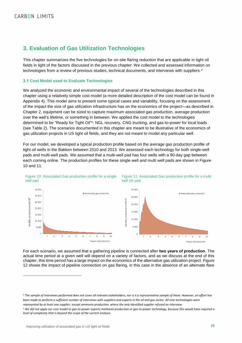
For our model, we developed a typical production profile based on the average gas production profile of

tight oil wells in the Bakken between 2010 and 2013. We assessed each technology for both single-well

pads and multi-well pads. We assumed that a multi-well pad has four wells with a 90-day gap between

each coming online. The production profiles for these single well and multi well pads are shown in Figure

10 and 11.

Figure 10: Associated Gas production profile for a single well pad

Figure 11: Associated Gas production profile for a multi well (4) pad

For each scenario, we assumed that a gathering pipeline is connected after two years of production. The actual time period at a given well will depend on a variety of factors, and as we discuss at the end of this chapter, this time period has a large impact on the economics of the alternative gas utilization project. Figure 12 shows the impact of pipeline connection on gas flaring, in this case in the absence of an alternate flare

d The sample of interviews performed does not cover all relevant stakeholders, nor is it a representative sample of these. However, an effort has

been made to perform a sufficient number of interviews with suppliers and experts in the oil and gas sector. All nine technologies were

represented by at least one supplier, except ammonia production, where the only identified supplier refused an interview. e We did not apply our cost model to gas-to-power exports methanol production or gas-to-power technology, because this would have required a level of complexity that is beyond the scope of the current analysis.

24


reduction technology. We assumed that gas flaring will continue at a rate of 10% even after connection to the gas gathering system, due to operational disturbances at the wellhead and in the gas gathering system.

Figure 12: Hypothetical flaring at a single well with pipeline connection after two years and no other gas utilization technology

Figure 13 is a hypothetical example that shows how the production profile and the sizing and installation

timeline of the gas utilization technology interact over time. In this example, the gas utilization technology

is installed after approximately 1 year. Thus, the gas produced before this time must be flared; we

consider this “value lost from delayed implementation time” (light orange). After 1 year, a flare reduction

technology is installed; this technology captures and utilizes 9,000 Mcsf/month of gas that would otherwise

be flared (light green). Any gas that is produced over and above 9,000 Mscf/month must still be flared; we

consider this “value lost from lack of capacity” (orange). Finally, after about 5 years of operation,

production drops below 9,000 Mscf/month; after this period, the flare reduction technology will capture

nearly all produced gas, but it is larger than necessary. We consider the opportunity cost of having

oversized equipment “value lost from spare capacity” (dark green). We present a similar diagram for each

technology and scenario presented in the remainder of this chapter.

Figure 13: Hypothetical example of flare reduction technology application at a multi well pad

Value lost from delayed implementation time

Value captured by technology

Value lost from lack of capacity

Value lost from spare capacity

For each technology we also evaluated typical lean and rich gas streams (shown in Figure 14). These two

scenarios aim to be representative of the conditions in tight oil production, but the gas composition at a

Pipeline Connection

25


particular site in the Bakken or the Eagle Ford may be quite different due to a high degree of variability in

these basins.

Figure 14: Range of gas compositions used for the model

Lean Gas Composition Rich Gas Composition

It is important to note that this model is intended to be illustrative and was not used to fully explore all the

ways that these technologies can be deployed. For each technology, we investigated the net present

value (NPV) as a function of the size of gas utilization infrastructure for the typical single-well pad and

multi-well pad discussed above. Only single-sized deployments were modeled – scaling in series (see Fig.

9) was not explored. As discussed below, NGL recovery can only utilize a limited portion of an associated

gas stream, but the residual gas remaining after NGL recovery can feasibly be utilized by other

technologies. However, we did not model pairing of technologies in this way (with the exception of

considering revenues from sale of the heavy hydrocarbons that are separated during compression of CNG

without additional equipment). Finally, the simplified model does not capture intraday variability, which will

reduce the amount of gas captured by equipment of any given size.

However, the model illustrates the overall general economics of deploying these technologies at the

different types of production facilities. Below, within the discussion of these technologies, we present data

for costs/NPV for purchase of systems, with the size of the system selected by maximizing NPV. The

model can also assess the economics of rental systems, but in the interest of clarity, we present those

results among several variability factors at the end of this chapter. Depending on the technology type, the

characteristics of the well, and financial factors such as cost of capital, which will vary greatly among well

operators, renting may improve or worsen the economics of the project.

The reduction in flaring and abatement cost per ton of avoided GHG (CO2eq) emissions at the maximum-

NPV size is also presented for each technologyf. For simplicity, we generally only considered the change

in GHG emissions at the well site – secondary effects such as reductions in transport emissions (due to

displacing diesel fuel consumption with associated gas) or increases in transport emissions (for CNG

f Abatement cost per ton of avoided CO2 equivalent includes methane emissions associated with incomplete combustion at flare. We assume a 98.5% combustion efficiency

26


trucking) are not considered. Details on the emissions sources included in this calculation are noted for

each technology.

Flaring produces significant pollution, including carbon dioxide and pollutants such as NOx and VOC that

are detrimental to local air quality. Therefore, from an overall societal perspective, it may be appropriate

to install infrastructure larger than the maximum-NPV size when larger sizes will reduce pollution at low

cost. For example, as discussed in Section 3.7.4, in certain cases larger installations can reduce flaring

significantly more than an installation sized to maximize NPV, while remaining profitable for well owners.

In Section 3.7.4, we also discuss the abatement costs per ton of avoided pollutants such as VOC and NOx

for some technologies.

Gas gathering systems

Gas gathering systems have historically been the main, and often only, means of capturing associated

gas and bringing it to market. These systems are usually several miles of low pressure (20-25 psi) suction

pipelines made of steel or high grade plastic, which collect gas mainly from the oil and gas separators and

treaters, where average maximum field pressure is higher (45-55 psi). This pressure difference makes the

gas flow from the well into the gas gathering system.

In the case of a single well located near existing infrastructure (< 5 miles), investments in gas gathering

are still the most common option for associated gas utilization. However, due to other technical,

geographical and commercial factors described in Chapter 2 (and summarized below), gas gathering

systems might not be connected to wells, especially in the early months of production—when associated

gas production is often at its peak.

Table 3: Gas Gathering Summary

Advantages

Disadvantages

Te

chnic

al

Proven, reliable technology: Pipelines can adapt to small and large volumes.

Capacity: New high producing wells are able to route large volumes of gas into gas gathering systems.

Technical safety: Flaring events may still be necessary for technical safety.

Gas gathering availability: Gas gathering system capacity constraints and availability issues lead to significant flaring of gas from wells on pipeline networks in the Bakken. (Ref to section 1.3.1 for more details)

Com

merc

ial

Fast payback: Cost per well of large developments is low and several mid-stream contractual agreements are available.

Readily scalable to multiple wells: Several wells together can justify longer pipelines and centralized compression facilities.

Waiting for pipeline to come: Pipeline development timing can be long, due to right of ways and permitting processes.

Profitability highly depends on the gas stream volumes: Revenue is tied to gas stream volumes and pipeline and market capacity.

Collaboration or contractual agreements issues between well operators and gas processing plant owners: If the gas processing plants are getting rich gas but paying lean gas price, tight oil operators are losing that value while gas processing plants may flare in excess due to operational issues on gas gathering systems. (Ref to section 1.3.2 for more details)

Compression costs: Inefficient deployment of infield and centralized compression systems may carry significant operating expenses to the gas gathering system.

Geogra

phic

When lines are already located nearby wells (less than a mile distance), hook-up can be rapid and simple.

High capital expenses for remote, small-scale, isolated well pads: Gas gathering development costs are very high for single well developments and the “last mile” cost is also considerable if right-of-ways are required.

27


Natural Gas Liquids (NGL) Recovery31

Natural Gas Liquids (NGLs) are valuable, naturally occurring components of associated gas, and include

hydrocarbons that are heavier than methane (C1), including ethane (C2), propane (C3), butanes (C4), and

pentanes or natural gasoline (C5). NGL recovery involves separating heavier NGLs from lighter gas.

Each hydrocarbon play will present a different range of liquid content in the gas. The liquid constituents

can be removed (condensed) as a liquid from raw natural gas and marketed. The remaining lean

“residual” gas (mainly methane) can be used to power NGL recovery equipment, gathered through

conventional gas gathering systems, used productively in another way (e.g., CNG trucking, generating

power, etc.), or, as a last resort, flared. Thus, NGL recovery can be paired with other technologies

discussed in this report that can utilize the residual gas.

A variety of NGL recovery technologies are available; these technologies vary in effectiveness. Simpler

and cheaper technologies, such as “BTU stripping towers” that use a simple expansion approach will only

remove the heaviest NGLs - C5 and heavier compounds – from raw gas. More expensive and complex

cryogenic technology is required extract ethane from raw gas. The appropriate technology depends upon

the intended use of residual gas and the available means to get NGLs to market. In general we can

summarize the levels of NGL separation for important constituents of raw associated gas as follows:

Table 4: NGL Constituents

Constituent

Ethane (C2)

If separated along with the rest of NGLs,

Decreases the price per gallon of the recovered NGLs

Increases substantially the total volume NGLs recovered

Separation of the ethane from methane is relatively difficult and in general requires a cryogenic unit, making it much more expensive32

If left in the natural gas stream,

Decrease purity and increase heating value of natural gas stream, making it more challenging for gas utilization options like power generation or LNG. Note that some residual ethane is typically acceptable (“pipeline quality” natural gas typically contains several percent ethane)

Main NGLs (C3-C5) No potential issues

Richer gas (C5+)

Larger refrigeration duties, larger heat exchange surface

Higher capital cost

They can be trucked to NGL pipelines or gas processing plants. If allowed, they can be blended into the crude, increasing oil production

Can be marketed separately, with high market prices

Various systems for NGL recovery are available, which recover various amounts of NGLs at very different

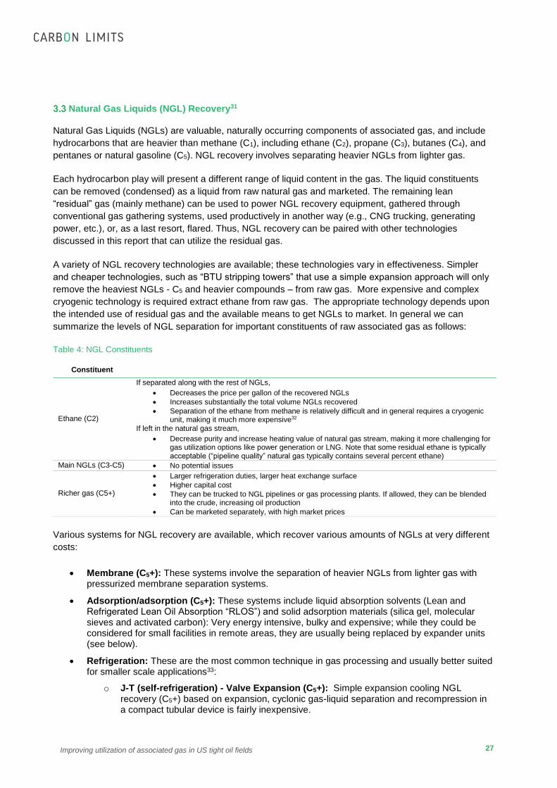
costs:

Membrane (C5+): These systems involve the separation of heavier NGLs from lighter gas with pressurized membrane separation systems.

Adsorption/adsorption (C5+): These systems include liquid absorption solvents (Lean and Refrigerated Lean Oil Absorption “RLOS”) and solid adsorption materials (silica gel, molecular sieves and activated carbon): Very energy intensive, bulky and expensive; while they could be considered for small facilities in remote areas, they are usually being replaced by expander units (see below).

Refrigeration: These are the most common technique in gas processing and usually better suited for smaller scale applications33:

o J-T (self-refrigeration) - Valve Expansion (C5+): Simple expansion cooling NGL recovery (C5+) based on expansion, cyclonic gas-liquid separation and recompression in a compact tubular device is fairly inexpensive.

28


o External Refrigeration (C3+): Simplest and most direct process passing counter-current gas streams through a gas-to-gas heat exchanger and then applying external mechanical refrigeration. This technology can be applied with very rich gas stream, low inlet gas pressures and a wide range of gas rates. The capital and operation cost for this technology are generally relatively low, but ethane is usually not separated from the gas stream and propane is only partially separated. Mechanical (external) refrigeration NGL recovery (C3+) has usually a very short payback time.

o J-T (self-refrigeration) - Low Temperature Separation (LTS) (C3+): These technologies are more suitable when the inlet gas pressure is very high (automatically-operated JT unit). The capital and operating costs are higher than for the external refrigeration technology.

o J-T (self-refrigeration) - Cryogenic or Expander (turbine) (C2+): These technologies can be applied to leaner gas streams, with low inlet gas pressures and very low gas production rates. Cryogenic turbo-expansion recovery is the most expensive NGL separation option. However, these technologies present a higher recovery of C3+ and are more flexible in terms of products specification, in particular if ethane recovery is desired.. If ethane is separated from associated gas, it is expensive to transport and store it due to its low boiling point and density. In general, ethane separation is not suggested unless the gas is going to be used in large gas turbines powering the grid, which require relatively lean gas34.

3.3.1 Application

We focused on NGL recovery technologies that are able to handle the typical volumes of associated gas

from tight oil production and can also be easily deployed. Based on these requirements we can conclude

that simple valve expansion system (C5+) and skid-mounted externally refrigerated systems (C3+) can be

a suitable options. Smallest units are in the range of 100 - 200 Mscf per day35, and industrial larger scale

systems start at 10,000 Mscf per dayg,36.

However, NGL recovery is not a complete gas utilization solution. For instance, a simple valve expansion

system only captures the heavier natural gas liquids components of the associated gas stream. If allowed,

these heavier components are usually blended into the oil while the remaining lean residual gas could be

utilized with other technology or flared. Alternatively, they can be trucked to NGL pipelines or gas

processing plants. Extracting liquids at well pads also eliminates or reduces the problem of liquids

condensing and impeding flow in gathering pipelines. However, commercial factors may limit the ability to

utilize this lean residual gas. For instance, some contracts between well operators and operators of gas

processing plants require the delivery of a certain amount of natural gas liquids, which are highly profitable

for the processerh.

In addition to separating liquids from the gas, making the gas composition more stable, NGL recovery

units act as a buffer for pressure and volume. NGL extraction is also required for hydrocarbon dew point

control and enables delivery of a gas with similar methane number over time. The methane number is a

product of the different constituent gases within the natural gas, particularly the proportions of methane,

ethane, propane, and butane. It gives an indication of the knock tendency of a fuel and it is an important

g NGL expanders of a scale smaller than approximately 25,000 mscfd are not commercially available; typically, approximately 75,000 mscfd is considered the low end of what is considered for commercial design. Recovering natural gas liquids from smaller streams would be performed using other technologies, such as straight refrigeration units or Joule-Thomson plants skid-mounted plants may be as small as 10,000 to 50,000 mscfd h Based on interviews with technology suppliers and stakeholders

29


factor when determining the appropriate engine version to select. Strict NGL removal (C3+) may produce

residual gas that, unlike raw associated gas, is suitable to fuel electrical generators or to be compressed

for CNG trucking (see sections below).

Suppliers of NGL recovery equipment are currently leasing equipment, so it is possible for operators to

lease various types and sizes of NGL recovery to match associated gas production over time. This

eliminates the upfront capital costs and maximizes natural gas recovery over time.

Pipeline connected flaring could be reduced by NGL recovery units installed on-site to solve insufficient

infield capacity and NGL pooling downstream if the agreement between the well pad operator and the

midstream company allows for NGL recovery from the associated gas stream. Even if the midstream

company does not allow NGL recovery from the portion of gas being sold to the midstream company, NGL

recovery could still be implemented on the portion of gas being flared to reduce overall flaring volumes.

Table 5: NGL Summary

Advantages Disadvantages

Te

chnic

al

Enables other solutions: NGL recovery allows certain other gas utilization options, such as power generation with lean gas

Reduces need for pigging (cleaning) of the gathering system

Emissions reduction: In addition to reducing CO2 emissions, NGL recovery generally reduces the emissions of black carbon and VOCs. By recovering the heavy components before flaring the gas, black carbon emissions are reduced.37 As gas flaring may not achieve 100% combustion efficiency, a share of the inlet gas is directly emitted to the atmospherei. When NGL recovery is installed, the gas stream contains significantly less VOCs and thus VOCs emissions are indirectly significantly reduced.

Partial solution: As mentioned above, the main disadvantage of this technology is that on its own, it is only a partial solution. In the absence of a means to export or utilize the lean gas, any residual gas not used to power compressors / refrigeration equipment will be flared.

Ethane is an issue both if it remains in the lean gas (limiting options for gas utilization) or it is taken out, which adds expense for separation, NGL storage, and NGL transport.

Gas liquids are expensive to handle, store, and transport compared to refined products. They require high pressure and/or low temperature to maintain liquid state for shipment and handling highly flammable – vapor “crawls” instead of rising; is heavier than air. They also need special trucks.

Buffer storage: In order to maximize economic potential, a sizable storage tank for gas is needed.

i Flares can achieve very low hydrocarbon emissions when properly sized, maintained and operated. On the other hand, poor design or poor maintenance can lead to significant emissions of unburned hydrocarbons. Additionally, flares will occasionally go out, and while unlit will vent gas.

30



Com

merc

ial

Scaling up or down: Mechanical systems are very flexible regarding scalability.

Contracts available for leasing equipment: Operators can lease NGL recovery equipment: Match size and type of NGL recovery equipment to the volume of the gas stream as it changes over time.

Economic attractiveness: Revenue is highly variable depending on gas composition and volume. As a result, the minimum pay-back time for a purely mechanical NGL unit can be as short as 60 days, while cryogenic NGL equipment can be in the range of 10-12 months, depending on the well productivity. On the other hand, pay-back times can go from 3 to 10 years for lean streams or poor well productivity. Leasing equipment can minimize investment risks.

Lean gas-to-power: If ethane levels are managed by separation, lean gas could power local loads and reduce diesel consumption or deliver power to the grid.

Increase well production with high value products: Full liquids recovery can allow an increase of up to 20% in the ratio of production to reserves (especially due to the ethane and propane volumes).

Promising market outlook: In both North Dakota and Texas, there is a currently a strong market for NGLs. In addition there is an important and increasing demand for ethane in Alberta,38 which could be met partially using the associated gas from North Dakota.

Scaling: Cryogenic systems are more challenging to scale.

Leasing conditions: Monthly payments may have to be carried out even when there is no NGL production.

Storage and trucking: New legislation in North Dakota (Approved Order 25417 in 9th December 2014) not allowing to blend crude into oil increases the level of logistic effort and associated investments (NGL storage tanks and NGL delivery services).

Geogra

phic

All types of NGL recovery could be profitable for wellpads located less than ~25 miles from existing infrastructure. Beyond 25 miles, NGL recovery of C5+ is nearly always profitable. For these remote wells, if increased levels of NGL recovery (C3+) are applied, the residual gas can be used to power local loads.

3.3.2 Cost Model

We modeled two forms of NGL recovery: simple valve expansion systems (C5+) and skid-mounted

externally refrigerated systems (C3+). C2+ recovery is not practical or economic for most oil field

applications due to economies of scale. NGL recovery systems are profitable at sites with rich gas, but,

not surprisingly, the systems will not be profitable and CO2 reductions will be costly at lean gas wells. We

present 4 scenarios for each technology (one for each gas production site type and gas composition

combination), and the operating design size of each scenario was chosen to maximize the NPV of the

system. In all of the rich gas cases, the systems can be built even larger to increase flare reduction /

pollution abatement, while still maintaining favorable economics.

Further details and assumptions on the cost model can be found in Appendix 4.

31


Simple Valve Expansion Systems (C5+): If the equipment is sized to maximize the net present value

(NPV) of the investment, flaring will only be reduced by 4%-5% for rich gas wells. At our model single well

site is not profitable due to NGL storage tank cost while at our model for multi well sites, systems sized

between 300 and 500 Mscfd would be profitable. If the C5+ are blended into the crude, the economics

would improve notably. These larger systems would achieve incremental higher flare reductions but they

would deviate from the optimum economic design. In general C5+ recovery is most economical for rich gas

streams, which have high levels of valuable heavy hydrocarbons. Payback period could be less than a

year according to suppliers of technology. Our assessment estimates that it will highly likely be less than 3

years for rich associated gas streams in multi-well developments.

Table 6: Summary of cost model for NGL recovery (C5+)

Single pad Multi well (4) pad

Rich case Associated Gas profile (inc. Pipeline connection after 24 months) j

Unit Lean Rich Lean Rich

Operating design size Mscf/day 100 100 400 400 Net back costk USD 245,000 245,000 740,000 740,000 NPV after 2 years USD -255,166 -50,803 -782,175 15,404 CO2eq reductions at flarel (98.5% eff. flare)

Tonnes CO2 114 439 412 1,668 % 1 % 4 % 1 % 4 %

Annualized abatement cost

USD/tCO2 4,269 239 4,278 -21

Pay-back time (without pipeline connection)

years

- - - ~2-3 years

Suppliers estimated pay-back time around 1 year for rich streams. Valve expansion technology (low investment cost) could pay-back in some months.

Influence of design for single and multi-well pads for rich streams Dashed lines represent the option of blending the NGLs into the crude Dotted lines represent the option of trucking the NGLs to appropriate markets

j Recovered gas is much smaller than the design size because the system must be designed based on the full associated gas stream, but only captures the heavy components of the stream. k Cost of purchasing equipment minus the estimated value of sales/re-use of equipment after project. l The calculation of CO2 reduction for NGL recovery systems does not include emissions from equipment used to separate NGLs from gas. C5+ separation equipment uses very little or no power.

32


Skid-Mounted Externally Refrigerated Systems (C3+): C3+ recovery requires a higher upfront cost, but

it is also profitable for single and multi-well pads with rich gas streams. They would remain profitable with

oversizing of 50% and Because C3+ separates a larger percentage of liquids from the gas stream than

C5+, flaring reductions are somewhat higher when sized to attain maximum NPV: between 14% and 18%

for wells with rich gas.

Table 7: Summary of cost model for NGL recovery (C3+)


Rich case Associated Gas profile (inc. Pipeline connection after 24 months) m


Operating design size Mscf/day 100 100 500 500

Net back costn USD 330,000 330,000 1,330,000 1,330,000

NPV after 2 years USD -293,409 17,301 -1,160,790 297,581

CO2eq reductions at flareo (98.5% eff. flare)

Tonnes CO2 422 1,639 1,846 7,538

% 5 % 14 % 6 % 18 % Annualized abatement cost

USD/tCO2 1,458 -23 1,408 -89


years

+ 10 years ~2-3 years ~10 years ~2 years

Suppliers estimated pay-back time around 1 year for rich streams.

Influence of design for single and multi-well pads for rich streams Dashed lines represent the option of blending the NGLs into the crude Dotted lines represent the option of trucking the NGLs to appropriate markets

m Recovered gas is much smaller than the design size because the system must be designed based on the full associated gas stream, but only captures the heavy components of the stream. n Cost of purchasing equipment minus the estimated value of sales/re-use of equipment after project. o The calculation of CO2 reduction for NGL recovery systems does not include emissions from equipment used to separate NGLs from gas. Our estimation is that C3+ separation equipment uses little power (10-40 HP). Calculations are based on de-scaling larger designs since C3+ equipment is usually found in larger installations (1-100 MMscfd).

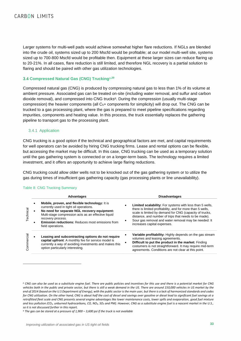
33


Larger systems for multi-well pads would achieve somewhat higher flare reductions. If NGLs are blended

into the crude oil, systems sized up to 200 Mscfd would be profitable; at our model multi-well site, systems

sized up to 700-800 Mscfd would be profitable then. Equipment at these larger sizes can reduce flaring up

to 20-21%. In all cases, flare reduction is still limited, and therefore NGL recovery is a partial solution to

flaring and should be paired with other gas utilization technologies.

Compressed Natural Gas (CNG) Truckingp,39

Compressed natural gas (CNG) is produced by compressing natural gas to less than 1% of its volume at

ambient pressure. Associated gas can be treated on-site (including water removal, and sulfur and carbon

dioxide removal), and compressed into CNG trucksq. During the compression (usually multi-stage

compression) the heavier components (all C5+ components for simplicity) will drop out. The CNG can be

trucked to a gas processing plant, where the gas is prepared to meet pipeline specifications regarding

impurities, components and heating value. In this process, the truck essentially replaces the gathering

pipeline to transport gas to the processing plant.

3.4.1 Application

CNG trucking is a good option if the technical and geographical factors are met, and capital requirements

for well operators can be avoided by hiring CNG trucking firms. Lease and rental options can be flexible,

but accessing the market may be difficult. In this case, CNG trucking can be used as a temporary solution

until the gas gathering system is connected or on a longer-term basis. The technology requires a limited

investment, and it offers an opportunity to achieve large flaring reductions.

CNG trucking could allow older wells not to be knocked out of the gas gathering system or to utilize the

gas during times of insufficient gas gathering capacity (gas processing plants or line unavailability).

Table 8: CNG Trucking Summary


Te

chnic

al

Mobile, proven, and flexible technology: It is currently used in tight oil operations.

No need for separate NGL recovery equipment: Multi-stage compression acts as an effective liquid recovery process.

Emission reductions: Reduces most emissions from field operations.

Limited scalability: For systems with less than 5 wells, there is limited profitability, and for more than 5 wells, scale is limited by demand for CNG (capacity of trucks, distance, and number of trips that needs to be made).

Sour gas removal and water removal may be needed: It increases capital expenses.

Com

merc

ial

Leasing and subcontracting options do not require capital upfront: A monthly fee for service model is currently a way of avoiding investments and makes this option particularly interesting.

Variable profitability: Highly depends on the gas stream volumes and leasing agreements.

Difficult to put the product in the market: Finding costumers is not straightforward. It may require mid-term agreements. Conditions are not clear at this point.

p CNG can also be used as a substitute engine fuel. There are public policies and incentives for this use and there is a potential market for CNG vehicles both in the public and private sector, but there is still a weak demand in the US. There are around 150,000 vehicles in US market by the end of 2014 (based on the U.S Department of Energy), with the public sector is the main user, but there is a lack of harmonized standards and codes for CNG utilization. On the other hand, CNG is about half the cost of diesel and savings over gasoline or diesel lead to significant fuel savings at a retrofitted fleet scale and CNG presents several engine advantages like lower maintenance costs, lower spills and evaporation, good fuel mixture and less pollution (CO2, unburned hydrocarbons, CO, NOX, SOX and PM). However, CNG as a substitute engine fuel is a nascent market in the U.S., so it is not discussed further in this report. q The gas can be stored at a pressure of 1,900 – 3,600 psi if the truck is not available

34



Geogra

phic

CNG trucking technology will work best at a well pad that is located close to a gas processing plant. At medium distance to market, CNG trucking could still be profitable for multi-well sites.

Not ideal for remote and wells more than 20-25 miles away from gas processing infrastructure.

3.4.2 Cost Model

Our cost model shows that the CNG option is profitable for both single and multi-well pads and for both

lean and rich gas, especially when the gas is rich. The heavier components (C5+) that drop out of the

multi-stage compressor are stored in NGL storage tanks until they are trucked to NGL pipelines or gas

processing plants. Blending them into the crude would increase the profitability of the project. NGL price is

“at the wellhead”.

In the cases evaluated, sizing the system for average production is economical, but it does not fully

capture emissions. We present 4 scenarios (one for each gas production and gas composition

combination), and the operating design size of each scenario was chosen to maximize the net present

value of the system. As shown in Table 9, systems can achieve a maximum NPV when sized at

approximately 200 Mscfd for single well pads and 600-700 Mscfd for multi well pads. Such systems can

reduce total flaring by over 90%. Systems can be even larger and remain profitable, up to 300 Mscfd for

single well pads and 850 Mscfd for multi well pads; these systems will remain economical, and achieve

even higher levels of flare reduction.

Total CO2 reductions for this technology, however, are slightly lower (65-85% reduction), due to the

emissions from the equipment needed to compress the natural gas.

Because of the portability of this technology, it can be rented on a temporary basis and the size can be

adjusted to match associated gas production. The renting option reduces flaring nearly as much as the

maximum size strategy, and it is profitable for the operator over a certain size (small wells may not be

profitable due to a standard daily fee). This option is not modeled directly, but it is another profitable option

for well operators.

35


Table 9: Summary of cost model for CNG trucking


Rich case Associated Gas profile (inc. Pipeline connection after 24 months)


Operating design size Mscf/day 200 200r 700 700 Net back costs USD 320,000 320,000 920,000 920,000 NPV after 2 years USD 95,023 679,282 621,634 2,796,320 CO2eq reductions at flare (exc. compression emissions)

tonnes CO2 7,047 10,542 26,406 39,592 % 91 % 93 % 95 % 96 %

Estimated CO2 reductions on-site (inc. compression emissionst)

% 65-85% 65-85% 70-85% 70-85%

Annualized abatement cost (exc. compression emissions)

USD/tCO2 -26 -126 -53 -159


years ~1.5 years ~1.5 year ~1.5 years ~1 year

Suppliers estimated the pay-back time between 1 and 2 years. Renting option should be profitable from the beginning for larger sites (Design of >400 Mscfd)

Influence of size for single well pads

Influence of size for multi-well pads

r Scaling down below 200 mscfd may be difficult (investment on truck capacity) s Cost of purchasing equipment minus the estimated value of sales/re-use of equipment after project. t We adjusted total CO2 reductions to account for total on-site CO2 emissions, including emissions from equipment that is needed to compress natural gas into CNG. Energy requirements for a multi-stage compression are fairly high and could amount to 1MW for large multi-well pads. Up to 10-25% of the gas compressed could be needed as fuel, reducing the final amount of emission reductions. However, we did not include diesel emissions from trucks used to transport the CNG fuel.

36


Gas-to-Power

3.5.1 Power generation technologies

A variety of technologies are available for power generation; reciprocating engines in bi-fuel configuration

and gas turbines (including micro turbines) are the most suitable technologies for associated gas for the

given scale of 0.2 - 10 MW40.

Reciprocating engines are internal combustion engines that are spark-ignited or compression-ignited.

They can be run on a mix of natural gas and diesel, through what is commonly referred to as dual fuel

technology41. The typical gas/diesel ratio for these systems is 60/40, although gas can be increased to

around 65%42,43. Reciprocating engines can achieve cost savings of up to 70% and reduce engine CO2

emissions by 20-30% during combustion by replacing diesel with natural gas44. Associated gas can be

used directly as fuel in reciprocating engines without NGL recovery, but some pretreatment (dewatering) is

still needed45. However, if the NGL levels in the gas are too high in the fuel mixture with diesel can cause

engine knocking (improper engine timing that can be destructive to the long-term health of the engine)46.

Variations in the gas composition and volume of associated gas may reduce the ability to replace diesel

fuel with gas47, limiting the potential applicability of the raw gas into the engines. So, dual-fuel engines

should not exceed 30% of diesel substitution with raw gas, while higher diesel substitution is possible

when NGLs are removed from gas before use as engine fuel.

Gas turbines used at well sites use similar technology as that found in gas power plants, just at a much

smaller scale. Gas turbines have more stringent requirements when it comes to gas stability, impurities,

and C3+ content, so NGL recovery is required prior to combustion. Gas sent to a turbine should be mainly

composed of methane and ethane, with only traces of propane. This can be accomplished through either

external refrigeration or turbo-expander technologies. In some cases, cryogenic refrigeration is needed so

a purer gas can be used for power applications in gas turbines with good performance and output, since

the flow is more stable and the fuel is already pre-compressed. Another option to keep a good fuel mix is

to use a gas reformer to convert heavier hydrocarbons (i.e. propane) into methane, but adding a catalytic

process is not as attractive because it usually requires water and it is expensive to purchase and operate.

There are also new technologies that allow a better pre-mixture, separation of components, and proper

vaporization of the fuel in the chamber, allowing commercial gas turbines to run on dual or multi-fuel

mode. These technologies are becoming available in the market, but they have not been commercially

proven on the context of tight oil production. We expect this option to be very attractive in the near future.

Microturbines could be seen as smaller versions of traditional gas turbines used in large power plants but

they differ substantially on their design, flows, pressures and temperatures. Microturbines can have fewer

stages and fuel burners and a more compact heat regeneration system. Typical power outputs of

microturbines range from 30 to 250 kW. Natural gas is the most common fuel, but other hydrocarbons,

such as kerosene, diesel or bio-fuels can be used as well.

3.5.2 Local Power Needs48

For wells that are not connected to the electric grid, gas-to-power technologies can be used to replace

diesel generations to meet well-pad power needs. Power is needed during oil well drilling and completion,

and during oil production. Wells require a large (but variable) amount of electricity during drilling and

completion, and they require a small (but stable) amount of electricity during production.

Drilling and completion operations last around one month on average. A substantial amount of equipment,

such as rigs, mast, supplementary structures (hydraulic power packs), mud pump, mud tanks, water

tanks, well control, boilers and drill strings, is needed, consuming between 1,000 to 4,000 gallons of diesel

37


per day. Power needs are estimated to be between 0.5 and 3.3 MWu. However, certain operations, like

fracking, can increase these needs up to 15 MW for several hours.

A variety of processes during productionv consume energy, but energy needs in production operations

are, in general, fairly low. Energy needs could be 0.1-0.15 MW for a typical well and 0.25 to 0.4 MW to run

multi-well sites49. Generating power for local use may be an appropriate option for installations of this

size, but given the continual variability of flow (which will go below the equipment’s fuel demand at times

as the well ages), it would generally be necessary to use back-up fuels, such as diesel, and bi-fuel

engines. Single well sites located at medium to long distances to existing infrastructure can use NGL

recovery and gas to local power with the remaining gas.

3.5.3 Grid integration and market

For wells that are connected to the electric grid, gas-to-power technologies can be used to generate

electricity that is sold to the market. It is possible to produce power at a very low costw, since the gas

would otherwise be flared (fuel cost is essentially zero).

While the price of natural gas generators will scale with size almost linearly, with limited economies of

scale, if a grid connection is needed, the roughly fixed cost of other required equipment (DC/AC

converters, auxiliaries, etc.) is a key element. As a result, it is more economical to install a single 3 MW

unit, than a set with more adjustable capacity (6 x 0.5 MW units).

Capital expenses, including auxiliaries, vary depending on the technology and the size. Our interviews and

research found that, as reference, we can take 600,000 USD for a 0.5 MW unit and 1.2 million USD for a 2

MW unit. Operational expenses are expected to be low. Gas-to-grid technologies may be uneconomical

for smaller units due to the high cost of auxiliary infrastructure (Balance of Plant), and it may be infeasible

due to the lack of long-term sales contracts (power purchase agreements) for power generated from

associated gas. Gas-to-Grid should only be considered for larger developments (> 1,000 Mscfd) from

several gas streams. Several wells (between 3 and 10) close to grid infrastructure, with gas pooled to

ameliorate the variability in production from single or small groups of wells, could supply power generation

to the grid.

3.5.4 Application

It is technically straightforward to use lean gas in engines. In cases where the associated gas stream is

rich, gas-to-power should be coupled with NGL recovery. Both NGL recovery units and generators are

available for lease, so operators should be able to lease equipment to meet needs at different stages of

production. If there is enough demand on site, this set up could yield substantial liquids revenue and

diesel fuel savings with a very short pay-back time. Sizing of equipment is complex and typically this

approach will not use all available associated gas.

On the other hand, given capital costs, the economics will be less favorable for single wells, wells with no

prior NGL recovery in place, and wells implementing power generation later than 1 year after initial

u Carbon Limits estimations (using 130 Btu / gallon of diesel, 3,413 Btu / kWh and 30% efficiency) v Such as oil lift, separation, semisubmersible pumps and pump jacks w Maintenance cost for small generators can be in the range of 0.002-0.03 $/kWh, including overhauls, according to different suppliers and bi-fuel substitution case studies

38


production. When these conditions are combined with a lack of on-site demand or integration to the grid at

a preferential price, power generation may be economically unfavorable.

In additional to the significant environmental and economic advantages of substituting gas that otherwise

would be flared for costly diesel, this approach also significantly reduces diesel transportation costs and

emissions.

Table 10: Gas to Power Summary


Te

chnic

al

Flexibility of choice: There are many available engines, allowing the operator to choose based on specific needs for each installation.

High uptime ratio: Maintenance and operation are usually low cost and require minimal downtime. Maintenance services are often available at all times.

Significant CO2 reductions: Generating power in controlled conditions with gas that would otherwise be flared gas yields almost 100% emission reductions. Additional reductions can be achieved if the gas is substituting diesel for powering drilling, completion or production operations. However, gas may still be flared if the power demand is insufficient.

Lean gas is preferred: Use of 100% raw gas limits the choice of engines, and a full substitution on diesel engines it is not yet possible, and presents multiple technical challenges. NGL recovery is needed since it acts as composition and volume buffer.

Scalability depending on technology: One technology will not suit the gas profile, therefore, a normal gas turbine will may have to be substitute by a micro-turbine at some point, or engines changed if not de-rated. Operators are moving to larger and larger units to supply multi-well pads (0.5 – 1 MW).

Coupling demand and supply: Fast changes in volumes and pressure may hinder equipment performance significantly if there is no buffer to drop the pressure down. A back-up system of liquid fuels like ethane and propane (from the NGL recovery or purchased from a gas processing plants) or diesel is usually needed to ensure supply. Operational practices are very important.

Com

merc

ial

Substantial fuel savings: Diesel consumption can be reduced up to 50% using no-cost associated gas, requiring little extra equipment (pretreatment) and investment.

Low cost electricity: Generating electricity from a cost-free fuel and selling it to the grid via a Power purchasing agreement and getting CERs at the same time it is a very attractive incentive to utilize gas in this context

Engagement: Larger oil and gas corporations may not be as interested on entering electricity delivery as smaller oil and gas producers, who want to squeeze every possible dollar out of their assets. In general, only when environmentally concerned employees or management tackle the issue of flaring are companies willing to collaborate and enter into gas utilization options like gas-to-power.

Planning: Oil and gas operators should have planned this option before starting operations, or even drilling. If not, delivery time of the larger units may be longer than expected, especially if they are customized to the gas composition. Grid integration may be bureaucratic and complicated, delaying the project.

Grid integration: The cost of Balance of Plant is a major barrier for small generators

Geogra

phic

Gas-to-power for Local Loads is an excellent choice for remote wells: If gas from several new wells remote from gathering systems can be tied together with stable gas input and back-up / buffering capacity, high diesel prices or high electricity prices, generating power can deliver substantial cost and emission savings, and, if power is sold, significant revenues from sales over several years.

Gas-to-power for Grid Connection requires electricity infrastructure, so not ideal for remote wells or even wells at medium distance to infrastructure.

39


3.5.5 Cost Model for power to local needs

We applied our cost model to three options for converting gas-to-power for local uses: reciprocating

engines, gas turbines, and microturbines. We did not apply the cost model to gas-to-power for grid-

connected loads. Such technology is only applicable for large multi well pads, and an analysis of the costs

of grid interconnection infrastructure is beyond the scope of our model.

For all gas-to-power for local power needs, scale is limited by power demand at the well site: energy

needs could be 0.1-0.15 MW for a typical single well pad and 0.25 to 0.4 MW to run multi well pads. This

translates to between 25-34 Mscf/day for single well pads and 50-100 Mscf/day for multi well pads. Thus,

for a production of 100-300 Mscfd, operators can reduce flaring by 5-20% by using associated gas-to-

power local demand on-site.

Based on the characteristics of tight oil wells that we have identified, including power needs, reciprocating

engine technology is the most economical of the three gas-to-power technologies, and gas turbines also

have a positive NPV under the parameters we have modeled. This technology can reduce flaring by 5-

10% at rich gas wells, and 15-20% at lean gas wells (since the substitution can be greater). Gas-to-power

applications require relatively lean gas, so wells with lean gas streams will be able to use a higher

percentage of their associated gas for on-site power generation, resulting in higher levels of flare

reduction. However, if the gas-to-power technology were paired with an NGL recovery system, a higher

percentage of the rich gas streams could be utilized, but this case is not modeled.

Total CO2 reductions associated with this technology, however, are even greater than these flare

reduction figures would suggest. Burning natural gas for on-site fuel releases less CO2 than burning the

diesel fuel it replaces. If we take into account fuel savings, the emissions reductions can almost double to

10-15% for rich gas wells and ~35% for lean gas wells. In addition, burning natural gas for on-site power

reduces the need to transport diesel fuel to the site, which reduces trucking emissions; however, this is not

included in our model.

Commercial models available (i.e. size) by vendors may limit the range of options available (and the

economic return) for the operator. For example, the minimum equipment size available may be larger than

local power needs, so operators may need to invest in oversized equipment. This scenario is not modeled

directly in our cost model.

40


Table 11: Summary of cost model for gas-to-power (Reciprocating engine)


Lean case Associated Gas profile (inc. Pipeline connection after 24 months)


Diesel substitution % 80 40 80 40

Operating design size (based on site demand)

Mscf/day 41 14 103 36

Net back costx USD 129,917 45,929 519,668 183,714 NPV after 2 years USD 114,778 40,576 494,376 174,773

CO2eq reductions at flare tonnes CO2 1,448 722 5625 2,815

% 18 % 6 % 19 % 7 % CO2eq reductions on sitey (inc. diesel substitution)

% 33% 12% 36% 13%

Annualized abatement cost (exc. diesel substitution)

USD/tCO2 -165 -118 -194 -137


years

1-2 years 1-2 years 1-2 years 1-2 years

Case studies and suppliers estimate the pay-back time up to 3-5 years. As stated, market availability of the equipment will highly probably oversize the equipment and increase pay-back time. If the substitution happens during drilling and completion or sites with large energy needs the pay-back time could become much shorter (~1 year). Fuel prices have a critical influence on the profitability. Lower diesel prices (< 3 USD/gallon) could increase pay-back time to ~3 years.

Influence of design:

Design is limited by power demand on site and market availability.

x Cost of purchasing equipment minus the estimated value of sales/re-use of equipment after project. y We adjusted total CO2 reductions to account for total on-site CO2 emissions, including reductions associated with replacing diesel with natural gas. However, we did not include reductions from trucks used to transport the diesel fuel.

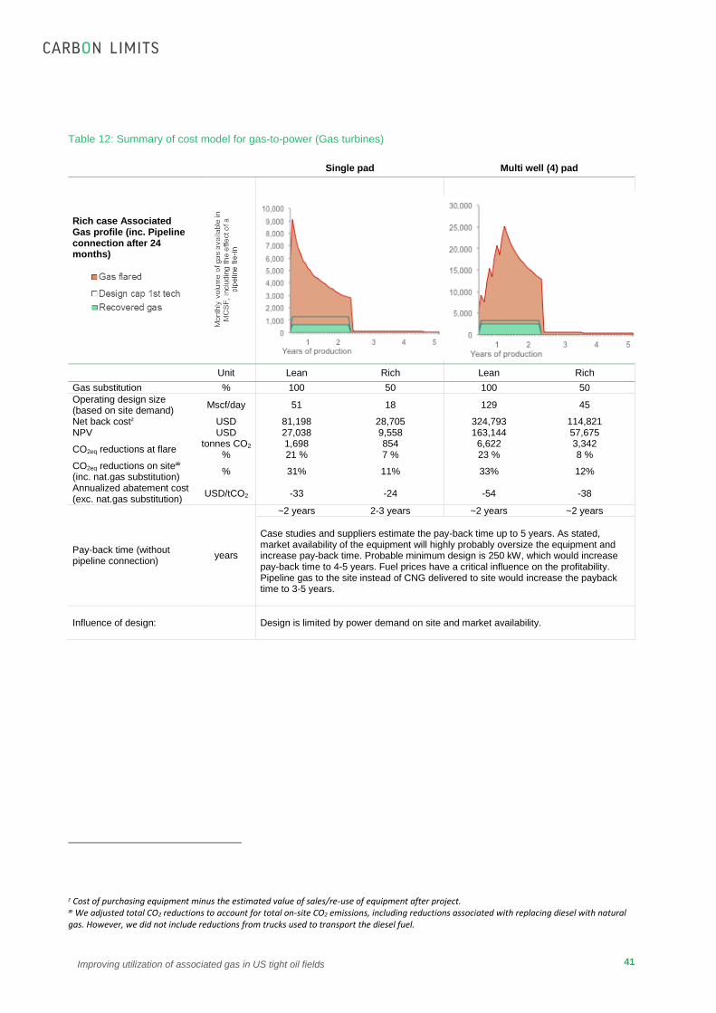
41


Table 12: Summary of cost model for gas-to-power (Gas turbines)




Gas substitution % 100 50 100 50


Mscf/day 51 18 129 45

Net back costz USD 81,198 28,705 324,793 114,821 NPV USD 27,038 9,558 163,144 57,675

CO2eq reductions at flare tonnes CO2 1,698 854 6,622 3,342

% 21 % 7 % 23 % 8 % CO2eq reductions on siteæ (inc. nat.gas substitution)

% 31% 11% 33% 12%

Annualized abatement cost (exc. nat.gas substitution)

USD/tCO2 -33 -24 -54 -38


years

~2 years 2-3 years ~2 years ~2 years

Case studies and suppliers estimate the pay-back time up to 5 years. As stated, market availability of the equipment will highly probably oversize the equipment and increase pay-back time. Probable minimum design is 250 kW, which would increase pay-back time to 4-5 years. Fuel prices have a critical influence on the profitability. Pipeline gas to the site instead of CNG delivered to site would increase the payback time to 3-5 years.



z Cost of purchasing equipment minus the estimated value of sales/re-use of equipment after project. æ We adjusted total CO2 reductions to account for total on-site CO2 emissions, including reductions associated with replacing diesel with natural gas. However, we did not include reductions from trucks used to transport the diesel fuel.

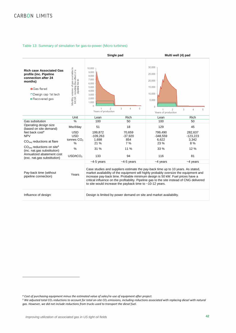
42


Table 13: Summary of simulation for gas-to-power (Micro turbines)




Gas subsitution % 100 50 100 50


Mscf/day 51 18 129 45

Net back costø USD 199,872 70,659 799,490 282,637 NPV USD -109,263 -37,920 -348,559 -123,223

CO2eq reductions at flare tonnes CO2 1,698 854 6,622 3,342

% 21 % 7 % 23 % 8 % CO2eq reductions on siteå (inc. nat.gas substitution)

% 31 % 11 % 33 % 12 %

Annualized abatement cost (exc. nat.gas substitution)

USD/tCO2 133 94 116 81


Years

~4-5 years ~4-5 years ~4 years ~4 years

Case studies and suppliers estimate the pay-back time up to 10 years. As stated, market availability of the equipment will highly probably oversize the equipment and increase pay-back time. Probable minimum design is 50 kW. Fuel prices have a critical influence on the profitability. Pipeline gas to the site instead of CNG delivered to site would increase the payback time to ~10-12 years.



ø Cost of purchasing equipment minus the estimated value of sales/re-use of equipment after project. å We adjusted total CO2 reductions to account for total on-site CO2 emissions, including reductions associated with replacing diesel with natural gas. However, we did not include reductions from trucks used to transport the diesel fuel.

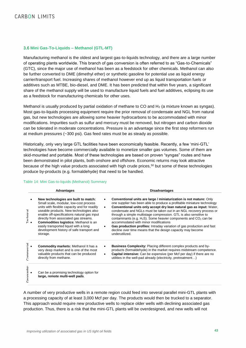
43


Mini Gas-To-Liquids – Methanol (GTL-MT)

Manufacturing methanol is the oldest and largest gas-to-liquids technology, and there are a large number

of operating plants worldwide. This branch of gas conversion is often referred to as “Gas-to-Chemicals”

(GTC), since the major use of methanol has been as a feedstock for other chemicals. Methanol can also

be further converted to DME (dimethyl ether) or synthetic gasoline for potential use as liquid energy

carrier/transport fuel. Increasing shares of methanol however end up as liquid transportation fuels or

additives such as MTBE, bio-diesel, and DME. It has been predicted that within five years, a significant

share of the methanol supply will be used to manufacture liquid fuels and fuel additives, eclipsing its use

as a feedstock for manufacturing chemicals for other uses.

Methanol is usually produced by partial oxidation of methane to CO and H2 (a mixture known as syngas).

Most gas-to-liquids processing equipment require the prior removal of condensate and NGL from natural

gas, but new technologies are allowing some heavier hydrocarbons to be accommodated with minor

modifications. Impurities such as sulfur and mercury must be removed, but nitrogen and carbon dioxide

can be tolerated in moderate concentrations. Pressure is an advantage since the first step reformers run

at medium pressures (~300 psi). Gas feed rates must be as steady as possible.

Historically, only very large GTL facilities have been economically feasible. Recently, a few ‘mini-GTL’

technologies have become commercially available to monetize smaller gas volumes. Some of them are

skid-mounted and portable. Most of these technologies are based on proven “syngas” routes and have

been demonstrated in pilot plants, both onshore and offshore. Economic returns may look attractive

because of the high value products associated with high crude prices,50 but some of these technologies

produce by-products (e.g. formaldehyde) that need to be handled.

Table 14: Mini Gas-to-liquids (Methanol) Summary


Te

chnic

al

New technologies are built to match: Small scale, modular, low-cost process units with flexible capacity and for readily useable products. New technologies also enable off-specifications natural gas input directly from associated gas streams.

Commodities logistics: Methanol is an easily transported liquid with a long development history of safe transport and storage.

Conventional units are large / miniaturization is not mature: Only one supplier has been able to produce a profitable miniature technology

Conventional units only accept dry lean natural gas as input: Water, condensate and NGLs must be taken out in an NGL recovery process or through a simple multistage compression. GTL is also sensitive to contaminants (e.g. H2S). Some heavier components and CO2 can be accommodated with minor modifications

Gas production profiles: Intraday variation of gas production and fast decline over time means that the design capacity may become underutilized.

Com

merc

ial

Commodity markets: Methanol It has a very deep market and is one of the most valuable products that can be produced directly from methane.

Business Complexity: Placing different complex products and by-products (formaldehyde) in the market requires midstream competence.

Capital intensive: Can be expensive (per Mcf per day) if there are no utilities in the well-pad already (electricity, pretreatment…)

Geogra

phic

Can be a promising technology option for large, remote multi-well pads.

A number of very productive wells in a remote region could feed into several parallel mini-GTL plants with

a processing capacity of at least 3,000 Mcf per day. The products would then be trucked to a separator.

This approach would require new productive wells to replace older wells with declining associated gas

production. Thus, there is a risk that the mini-GTL plants will be overdesigned, and new wells will not

44


compensate for the rapid decline rate at older wells. Overall, once methanol production technology

matures a bit more, it will be an attractive option for major tight oil developments.

We did not apply the cost model to methanol production. Such technology is ready for commercialization,

but it is still in the pilot stage. In addition, an analysis of the gas-to-liquids markets is beyond the scope of

our model.

General remarks and comparison

3.7.1 Technologies

In general we see CNG trucking and NGL recovery as the most suitable options for associated gas

utilization in economic terms. In addition, the use of associated gas for on-site power can also be

profitable, especially if the project lifetime is extended (pipeline connection takes longer than 2 years).

3.7.2 Variability factors

As we discuss in Appendix 4, we made a number of assumptions when designing our cost model. A

change in these assumptions could influence the results of our analysis. For example, if the capital

expenditure required is lower than what we assumed, project economics will improve. On the other hand,

if the gas utilization technology is not implemented until a year after production starts at a well, a large

amount of potential revenue will be lost and project economics will worsen. Other factors are more

ambiguous, e.g. for some technologies, single well pads have better economics, but for others, multi well

pads perform better, but as we have seen for each technology, economics are deeply correlated to the

optimization of design size.

We assessed the sensitivity of the model to changes in various parameters. We performed more than 200

different NPV simulations to cover a range of possible cases. Based on these simulations, factors have

been classified depending on the influence they can have on project economics:

Table 15: Expected influence of different variables on project profitability

Only/Mostly positive influence Depending on technology Only/mostly negative influence

Lowest estimation of CAPEX

Richer gas

Lower discount rate

Gathering pipeline connection takes more than 2 years

Single well or multi-well

Renting/leasing agreements

Oversizing equipment to the first months of production

Delay in 1 year of project implementation

3.7.3 Reduction of CO2 Emissions

As we alluded to above, selecting a design size that maximizes economic returns may not result in the

lowest level of flaring.

Figure 15 shows the relationship between emission reduction and abatement cost for CNG trucking. At

single well pads, the lowest abatement cost is at a 100 Mscfd design, but designs up to 400 Mscfd have

reasonable abatement costs per ton of carbon dioxide.

For multi well pads, the lowest abatement cost is at 500 Mscfd, but abatement costs remain negative even

as the system is scaled up.

45


Figure 15. Abatement Cost (left axis) and emission reductions (%) for single and multi-well pads with lean gas composition for different design of the CNG trucking options

3.7.4 Reduction of VOC and NOx Emissions

In addition to the potential reductions in GHG emissions presented in this report, application of gas utilization technologies would also reduce emissions of pollutants that degrade air quality such nitrogen oxides (NOx), volatile organic compounds (VOC), and particulate matter (PM). Here, we consider reductions, and abatement cost per ton of avoided pollutants, for NOx and VOCaa.

Table 16 presents key metrics related to investments in gas utilization technologies for some selected cases presented earlier in this report. It compares the economic returns to the reduction of VOC and NOx emissions from the flare.

These cases are optimized to maximize NPV for each technology, well size, and gas composition

combination. All of these cases have positive NPVs, so the VOC and NOx abatement costs are

consequently negative.

aa As discussed above, these gas utilization technologies all use some amount of associated gas on site as engine fuel for compressors or generators, and in some cases displace other onsite engine fuel (diesel). The additional and displaced engines emit NOx and VOC, but in significantly smaller amounts per unit of fuel burned than flares (assuming the use of modern engines with emission controls), so this analysis only considers emissions from flares.

46


Table 16: Key parameters related to VOC and NOx reduction for selected cases.

Technology Size Gas

Composition

Design

Max

NPV

Flare

reduction

Net

Present

Value

VOCbb NOxcc

Mscf/

day % USD tVOC

USD/tVOC

reduced tNOx

USD/tNOx

reduced

NGL recovery C5+ Single well Rich gas 100 4% -50,084 3 18,078 11 4,735

NGL recovery C5+ Multi-well Rich gas 400 4% 15,404 10 -1,495 41 -378

NGL recovery C3+ Single well Rich gas 100 14% 17,301 11 -1,562 40 -432

NGL recovery C3+ Multi-well Rich gas 500 18% 297,561 41 -7,180 184 -1,614

CNG Trucking Single well Lean gas 200 91% 95,023 3 -34,455 178 -534

CNG Trucking Single well Rich gas 200 93% 679,282 14 -49,799 258 -2,635

CNG Trucking Multi-well Lean gas 700 95% 621,634 16 -39,439 667 -932

CNG Trucking Multi-well Rich gas 700 96% 2,796,320 59 -47,554 968 -2,888

It should be noted, however, that the abatement costs are sensitive to variations in NPV, and the NPVs of actual investment opportunities can vary greatly depending on site-specific characteristics, operations and market opportunities (e.g. gas composition, negotiated price of fuel deliveries, and delays in implementation). Table 17 presents a sensitivity analysis for the VOC and NOx abatement cost associated for one of the cases analyzed: CNG trucking applied to a single well with rich gas.

Table 17: Sensitivity analysis for CNG trucking in a single well with rich associated gas.

Factor Base case

value

Sensitivity

Analyzed Unit

NPV VOC NOx

USD tVOC USD/tVOC

reduced tNOx

USD/tNOx

reduced

Base case 200 - Mscfd 679,282 14 -49,799 258 -2,635

Sensitivity analysis – individual factors/parameters

1 CAPEX 320,000 780,000 USD 224,603 14 -16,466 258 -258

2 Value of CNG 7.85 4.17 $/Mscf 73,057 14 -5,356 258 -283

3 Oversizing 200 400 Mscfd 503,978 18 -28,502 271 -1,860

4 Time of pipeline tie-in 25th 13th month 362,694 8 -44,785 155 -2,854

5 Delay start-up of 6 months 1st 7th month 365,167 11 -31,530 167 -2,173

Sensitivity analysis – combination of multiple factors/parameters

1+2 CAPEX + VALUE

See above

-381,623 14 27,977 258 1,480

1+4 CAPEX + PIPELINE -91,986 8 11,358 155 594

2+5 VALUE + DELAY -44,356 11 3,862 167 266

bb For VOC from flares, we assume 98.5% VOC destruction efficiency, consistent with data supporting EPA’s analysis of flare operation (see AP 42, Fifth Edition, Volume I Chapter 13: Miscellaneous Sources Industrial Flares. Available at: http://www.epa.gov/ttn/chief/ap42/ch13/final/dc13s05_8-19-14.pdf). Note that while the destruction efficiency of flares, while lit, may be considerably higher than 98.5% (see Caulton, et al. Methane Destruction Efficiency of Natural Gas Flares Associated with Shale Formation Wells. Environ. Sci. Technol., 2014, 48 (16), pp 9548–9554. Available at: http://pubs.acs.org/doi/abs/10.1021/es500511w) the emissions factor must also take into account the tendency for flares to go out due to high winds, intermittent flow, etc. Emissions may be significant in the period before the flame is re-lit. These emissions factors are sensitive to the VOC content of associated gas and design and operation of the flare. Poorly designed and/or operated flares can have a large impact on the emissions; an inefficient flare will emit significantly higher levels of VOC than we assume here. cc For NOx from flares, we used an emissions factor of 2.9 lb NOx per MMBtu gas flared, based on EPA’s recommended emissions factor for industrial flares. (AP 42, Fifth Edition, Volume I Chapter 13: Miscellaneous Sources Industrial Flares. Table 13.5.2.) The calorific values of rich gas was assumed to be 1,593 MMBtu per MCF, and lean gas was assumed to be 1,103 MMBtu per MCF.

47


Gas utilization projects are normally seen primarily as resource preservation and CO2 reduction measures or even business opportunities, rather than VOC or NOx reduction measures per se. This is illustrated by the relatively high initial capital requirements per ton of VOC that can be reduced compared to other VOC reduction measures, e.g. methane leak avoidance.

However, an investment in gas utilization technologies with positive NPV presents a good opportunity to minimize VOC and NOx emissions associated with tight oil production. It should be stressed that base cases with poorly designed and/or operated flares can increase the VOC and NOx reduction potential. Furthermore, even some cases with a negative NPV, including overdesigning equipment to capture a larger share of pollutants, may still reduce VOC and NOx emissions at reasonable costs—below $5,000 per ton of avoided emissions. Below (Figure 16) is an illustration of the effect of sizing versus abatement costdd.

Figure 16: Net Present Value vs. NOx abatement cost for NGL Recovery C3+ at multi well pad with rich gas.

Flare Reduction (%) 5 % 8 % 12 % 15 % 18 % 19 % 20 % 21 % 21 % 21 % NOx Reduction (tonnes)

51 87 122 156 184 203 213 216 217 217

dd Systems sized at and above the maximum average daily output of the well pad have a net cost, but the costs are reasonable. As we discussed in Section 2.1.3, associated gas production experiences a high level of intraday variation, which is not captured in our model. So, actual production would spike above the maximum average daily output for short periods, especially during the highest production periods of the well pad. Equipment scaled at the maximum daily average would not capture these gas spikes.

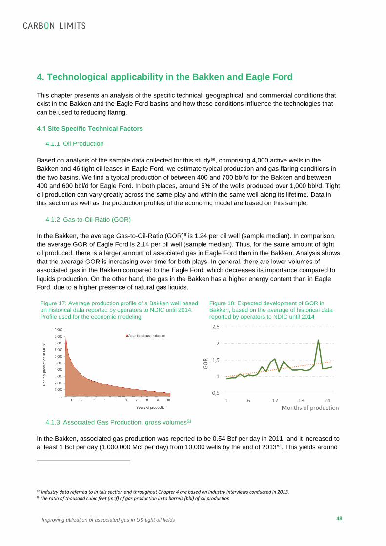
48


4. Technological applicability in the Bakken and Eagle Ford

This chapter presents an analysis of the specific technical, geographical, and commercial conditions that

exist in the Bakken and the Eagle Ford basins and how these conditions influence the technologies that

can be used to reducing flaring.

Site Specific Technical Factors

4.1.1 Oil Production

Based on analysis of the sample data collected for this studyee, comprising 4,000 active wells in the

Bakken and 46 tight oil leases in Eagle Ford, we estimate typical production and gas flaring conditions in

the two basins. We find a typical production of between 400 and 700 bbl/d for the Bakken and between

400 and 600 bbl/d for Eagle Ford. In both places, around 5% of the wells produced over 1,000 bbl/d. Tight

oil production can vary greatly across the same play and within the same well along its lifetime. Data in

this section as well as the production profiles of the economic model are based on this sample.

4.1.2 Gas-to-Oil-Ratio (GOR)

In the Bakken, the average Gas-to-Oil-Ratio (GOR)ff is 1.24 per oil well (sample median). In comparison,

the average GOR of Eagle Ford is 2.14 per oil well (sample median). Thus, for the same amount of tight

oil produced, there is a larger amount of associated gas in Eagle Ford than in the Bakken. Analysis shows

that the average GOR is increasing over time for both plays. In general, there are lower volumes of

associated gas in the Bakken compared to the Eagle Ford, which decreases its importance compared to

liquids production. On the other hand, the gas in the Bakken has a higher energy content than in Eagle

Ford, due to a higher presence of natural gas liquids.

Figure 17: Average production profile of a Bakken well based on historical data reported by operators to NDIC until 2014. Profile used for the economic modeling.

Figure 18: Expected development of GOR in Bakken, based on the average of historical data reported by operators to NDIC until 2014

4.1.3 Associated Gas Production, gross volumes51

In the Bakken, associated gas production was reported to be 0.54 Bcf per day in 2011, and it increased to

at least 1 Bcf per day (1,000,000 Mcf per day) from 10,000 wells by the end of 201352. This yields around

ee Industry data referred to in this section and throughout Chapter 4 are based on industry interviews conducted in 2013. ff The ratio of thousand cubic feet (mcf) of gas production in to barrels (bbl) of oil production.

49


100 Mcf per day per well. Future production of associated gas may increase to 1.4-2.1 Bcf per day in 2017

and 2-3.1 Bcf per day in 202553,gg.

In the Eagle Ford associated gas production was 1.91 Bcf per day in 2009 and accounted for 9.15% of

total US associated gas production of 20.84 Bcf per day, according to the Texas Railroad Commission. By

2012, output of associated gas reached 3.34 Bcf per day, which comprised 15.2% of total US associated

gas production of 21.99 Bcf per day54. Texas (onshore) is estimated to have the largest volumes of natural

gas flared and vented in the US; the majority of gas produced in Texas is from gas wells, while 14% is

associated gas produced at oil wells. Most of the gas produced is either marketed (>90%) or re-

pressurized for re-injection (~7%). Limited amount of gas is flared or vented (0.4%). A small percent of all

gas produced is flared, however, the percent would be higher if we only considered the percent of gas

flared from oil wells rather than combining flaring at both oil and gas wells. We estimate that associated

gas production in the Eagle Ford from tight oil developments is at least 1 Bcf per day and likely more than

2 Bcf per day. There is no clear way to forecast associated gas production, but based on expected

increase in oil production and an increasing GOR over time, we can expect an increase in associated gas

production in the next several years.

4.1.4 Associated gas production, time-lapse distribution

Data for the Bakken show that production rates on average drop to 36%-46% of peak production after 12

months, and further to 14% and 7% of peak production after 24 and 36 months respectively. Data for the

Eagle Ford indicates similar decline rates. Distributions of monthly production after 2, 12, 24, and 36

months of production are illustrated in Figure 21. Less than 5% of the wells in the Bakken produced over

500 Mcf per day of associated gas after one year of production. An average Bakken well will probably

produce around 100 Mcf per day on average after one year of production, with 70% of wells producing

from 30 – 300 Mcf per day.

Gas utilization technologies must be designed and optimized to account for this declining gas production

and variations in associated gas recovery rates. This is particularly critical when associated gas is used for

electricity generation; when associated gas is used to provide electricity for local loads, diesel fuel will

usually be used as a backup fuel. The “balancing act” of managing a variable supply of gas input with

customers’ need for a reliable volume of gas makes associated gas recovery utilization difficult, especially

if gas is used to deliver electricity to the grid, and thus gas to power for grid applications are rarely

appropriate in the Bakken or the Eagle Ford, except in some large, multi-well developments.

gg The EIA has presented figures for the total amount of natural gas annually produced, flared or vented in the US. It is not a straightforward task to disaggregate these figures to obtain associated gas flare estimates related to different categories of reserves (e.g. production of tight oil formations). In order to provide an assessment of the flaring conditions in the different states with current or potential tight oil production, we have coupled gas flared or vented statistics provided with the gas withdrawals by type of product on each state.

50


Figure 19: Distribution of associated gas production at different stages of development from wells in the Bakken based on selected sample

4.1.5 Associated gas production, gas quality

Associated gas from tight oil wells in the Bakken is usually very rich in NGLs (6-12 gallons per Mcf,

minimum heat content of 1,300-1,500 BTU/scf). A typical Bakken well yields around 30-50 barrels of NGLs

per day. It is typically low in sulfur.

The Eagle Ford associated gas is not as rich as that from the Bakken (4-9 gallons per Mcf, heat content

estimated around 1,200 BTU/scf), but due to higher gas production volumes in the Eagle Ford, a typical

well can yield close to 60 barrels of NGLs per day. It is also typically low in sulfur.

4.1.6 Associated gas flaring, gross volumes

In North Dakota gas flared or vented is directly linked to tight oil developments. In August 2013,

associated gas flaring was around 29%, of which 55% was from isolated wells, while the remaining 45%

was from already connected wells. The average for 2013 is shown in Figure 20: . Pipeline connected well

flaring has been more of an issue in central and southwest counties (Slope and Bowman) in North Dakota,

while lack of pipelines in northeast counties (Renville, Bottineau and Ward) has resulted in flaring from

isolated wells.

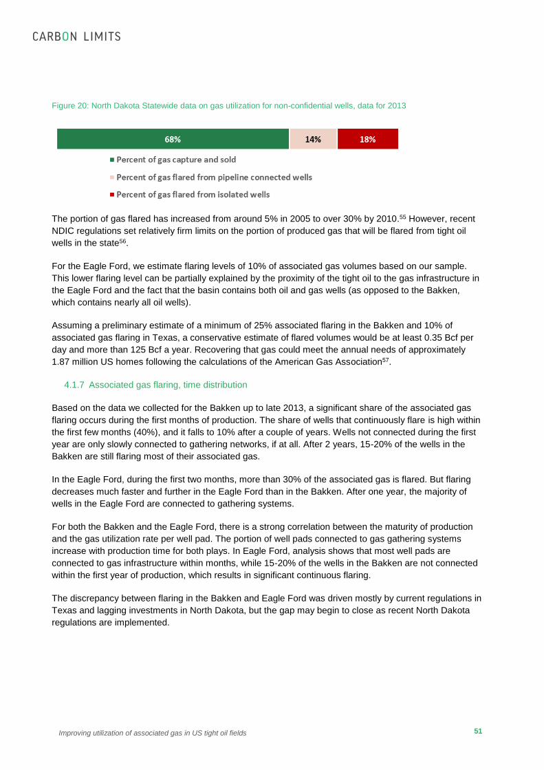
51


Figure 20: North Dakota Statewide data on gas utilization for non-confidential wells, data for 2013

The portion of gas flared has increased from around 5% in 2005 to over 30% by 2010.55 However, recent

NDIC regulations set relatively firm limits on the portion of produced gas that will be flared from tight oil

wells in the state56.

For the Eagle Ford, we estimate flaring levels of 10% of associated gas volumes based on our sample.

This lower flaring level can be partially explained by the proximity of the tight oil to the gas infrastructure in

the Eagle Ford and the fact that the basin contains both oil and gas wells (as opposed to the Bakken,

which contains nearly all oil wells).

Assuming a preliminary estimate of a minimum of 25% associated flaring in the Bakken and 10% of

associated gas flaring in Texas, a conservative estimate of flared volumes would be at least 0.35 Bcf per

day and more than 125 Bcf a year. Recovering that gas could meet the annual needs of approximately

1.87 million US homes following the calculations of the American Gas Association57.

4.1.7 Associated gas flaring, time distribution

Based on the data we collected for the Bakken up to late 2013, a significant share of the associated gas

flaring occurs during the first months of production. The share of wells that continuously flare is high within

the first few months (40%), and it falls to 10% after a couple of years. Wells not connected during the first

year are only slowly connected to gathering networks, if at all. After 2 years, 15-20% of the wells in the

Bakken are still flaring most of their associated gas.

In the Eagle Ford, during the first two months, more than 30% of the associated gas is flared. But flaring

decreases much faster and further in the Eagle Ford than in the Bakken. After one year, the majority of

wells in the Eagle Ford are connected to gathering systems.

For both the Bakken and the Eagle Ford, there is a strong correlation between the maturity of production

and the gas utilization rate per well pad. The portion of well pads connected to gas gathering systems

increase with production time for both plays. In Eagle Ford, analysis shows that most well pads are

connected to gas infrastructure within months, while 15-20% of the wells in the Bakken are not connected

within the first year of production, which results in significant continuous flaring.

The discrepancy between flaring in the Bakken and Eagle Ford was driven mostly by current regulations in

Texas and lagging investments in North Dakota, but the gap may begin to close as recent North Dakota

regulations are implemented.

52


Figure 21: Share of flaring in different months of production per well in the Bakken and Eagle Ford

Bakken wells Eagle Ford Leases

These graphs show the trends in flaring in the Bakken and the

Eagle Ford. The green, orange, and red colors (left axis) show

the share of wells that have no flaring, pipeline connected well

flaring, and continuous flaring.as a function of the number of

months in production. The red line (right axis) shows the

cumulative share of gas flared as a function of months of

production.

Percent of Gas Flared:

100% Isolated Well/Continuous Flaring

75% - 99%

Pipeline Connected Flaring 50% - 75%

25% - 50%

1% - 15%

0% No Flaring

4.1.8 Associated gas flaring, volume distribution

The associated gas volume on an average lease in the Eagle Ford is approximately double associated

gas production from an average lease in the Bakken. This occurs for several reasons: the Eagle Ford has

an average GOR that is more than twice that of the Bakken and because a lease in the Eagle Ford

typically contains more wellpads than a typical lease in the Bakken. Data from both the Bakken and the

Eagle Ford show that well pads with limited gas production (< 1,000 Mcf per day) are less likely to be

connected to gathering systems than larger production sites. Our analysis of flaring in the Bakken and the

Eagle Ford revealed the following:

Small sources of associated gas (< 1,000 Mcf per day) have more cases of continuous flaring (10-20% of the wells for both the Bakken and the Eagle Ford).

The larger the volumes of associated gas (> 1,000 Mcf per day), the higher the share of pipeline connected flaring.

Very large flare events are intermittent and uncommon (<5% of the time). They account for approximately 20-35% of the gas flared resulting from insufficient pipeline capacity.

Large flares are important to solve the problem. For example, in December 2011, the majority of the Bakken wells flared less than 300 Mcf per day, but the wells flaring over 300 Mcf per day flared accounted for half of the total volumes flaredhh.

hh A well in the Bakken may be alone (isolated, single well pad), in the same well pad as other wells (multi well pads) or surrounded by other single well pads.

0%

20%

40%

60%

80%

100%

0 %

20 %

40 %

60 %

80 %

100 %

1 6 12 18 24

Ave

rag

e sh

are

of

the

ga

s Fl

are

d

% o

f w

ells

Months of production

53


Figure 22: Level of flaring and cumulative flaring of all sample wells (different stages of development), sorted by gas produced in Mcf per day (per well in the Bakken and per lease in Eagle Ford.

These graphs show the trends in flaring in the Bakken and the

Eagle Ford. The green, orange, and red colors (left axis) show

the share of wells that have no flaring, pipeline connected well

flaring, and continuous flaring.as a function of the total gas

produced. The red line (right axis) shows the cumulative share

of gas flared as a function of total gas produced.



75% - 99%


25% - 50%

1% - 15%

0% No Flaring

4.1.9 Technology application related to technical factors

Table 18 summarizes three important technical factors for each gas utilization technology. All technologies

require removal of C5+, and gas-to-power systems work best with even leaner gas. NGL recovery and

gas-to-power for local loads are partial gas utilization technologies, while the other technologies can

capture nearly all of the associated gas that is produced.

Table 18: Technical assessment of selected technologies

Level of prior removal NGL

required and suggested Gas utilizationii

Scale

(Best fit)

Btu Stripping – valve

expansion (C5+)

External/JT

(Valve or Self-

ref. (C3+)

Cryogenic

(C2+) % →

Mcf per

day

Gas gathering 75 – 100 Any

NGL Recovery 20-35 Any

CNG Trucking 60-80 200-1,000

Gas-to-power (Local) 10-50 50-100

Gas-to-power (Grid) 0 – 100 >1,000

Mini GTL-MT Depends on the Supplier 80-100 >1.000

ii These numbers are preliminary and represent a range that could change if technical specifications change or technologies improve.

Bakken Wells Eagle Ford Leases

54


Site Specific Geographical factors

4.2.1 Distances between production sites

We studied the relationship of the distances between wells (how isolated well pads are) and flaring in the

Bakken:

Average distance between wells is 0.6 miles

50% of the wells are located within 0.12 mile of each other and can be assumed to be part of the same site (multi-well pads) (Figure 25)

The more isolated a well is, the less likely it is connected to other wells and gas gathering systems.

Well concentration: Wells that have wide spacing have a higher percentage of continuous flaring.

North Dakota data show that multi-well pads flare less than 30% of the produced associated gas, while isolated single wells flare up to 45% of the gas. Well concentrations are high and increasing in sweet spots (multi-well pads), and are lower in the frontiers of the basins

Figure 23: GIS representation of wells in a small area in North Dakota.

Figure 24: Wellpads (active or under development) in a random location in sweet spots counties in the Bakken and the Eagle Ford. Both images at the same scale

Figure 25: Flaring related to distance between wells in Bakken



75% - 99%


25% - 50%

1% - 15%

0% No Flaring

The Bakken has a lower concentration of wells than the Eagle Ford. In the Bakken, there are

approximately 120 is acres/well in the sweet spots but around 640 acres/well in the Sanish & Parshall

Fields. In comparison, in the Eagle Ford there are approximately 125-140 acres/well or even lower58. The

higher concentration in the Eagle Ford may be related to the larger share of multilateral horizontal wells.

Figure 24 show a Google EarthTM image of a small area of North Dakota with some of the wells that are

part of our sample.

25%

30%

35%

40%

45%

50%

0 %

20 %

40 %

60 %

80 %

100 %

0,3 0,6 0,9 1,2 1,6 Ave

rag

e a

sso

cia

ted

ga

s fl

are

d

% o

f w

ells

Distance in miles to the closest well

55


4.2.2 Distance to existing infrastructure

Proximity to existing infrastructure, including gas gathering systems and gas processing plants, facilitates

gas utilization.

Both the Bakken and the Eagle Ford have interstate gas pipelines, and the Eagle Ford also has intrastate

pipelines and two NGL pipelines. However, the most important infrastructure in terms of associated gas

utilization is presence of a gas gathering system to collect associated gas from each tight oil well. These

gas gathering systems must be connected to the individual well pads and gas processing plants with

sufficient capacity. Building these connections, and building out processing capacity, have been the

limiting factors in the expansion of gas gathering systems. Other limiting factors have been the permitting

process and issues with landowners and right-of-ways.

In the Bakken, a substantial number of miles of gas gathering infrastructure have been put in place, and

the pace of tie-ins has recently been on par with drilling activities. However, in order to avoid associated

gas flaring at wells with a gathering connection, there must be gas gathering capacity installed that is

larger than the average production rate, due to the high variability of associated gas production.

Furthermore, many of the more remote regions in northeast North Dakota still lack gas gathering

infrastructure.

In the Eagle Ford, tight oil leases are often relatively close to gas leases that are linked to the gas

gathering systems. Joint ventures and partnerships between energy companies in the area have

accelerated investment and brought much more infrastructure to the sites, especially when leases are

larger and the regulations are tighter.

4.2.3 Other geographical challenges

In rural environments such as western North Dakota and south Texas, it can be can be difficult and costly

to operate and maintain both electric grid and natural gas infrastructure.

Road networks are less developed in these regions, which could eventually pose a problem as some of

the gas utilization technologies like NGL trucking that, if widespread, would eventually increase already

heavily-congested secondary or dirt roads. Many of these roads have already seen a significant increase

in traffic from trucks carrying hydraulic fracturing equipment.

Harsh winter conditions are also a challenge for North Dakota operations. Several technologies may

reduce efficiency or require add-ons like waste heat recovery units. Trucking operations are feasible, but

challenging and accident prone during winter months. But, production also drops significantly during harsh

winter months, partially mitigating these issues.

4.2.4 Technology application related to geographical factors

In Table 19 we present an assessment of different technologies based on the geographical factors

reviewed, estimates on investment costs and the input from interviews with technology suppliers. In

general, gas gathering development over 10-15 km would be constrained to midstream companies

because the high investment cost. NGL recovery should be applicable to even isolated wells, especially

C5+ recovery. CNG trucking agreements are usually reserved to well pads that are within 25 miles from a

Gas Processing Plant. Satisfying local loads should not have a limitation in terms of geography. Actually, it

can benefit from very isolated locations where bringing diesel to site may be even more expensive. On the

other hand, gas-to-grid developments would need to be close to existing power networks or networks on

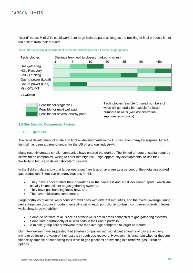
56


“island” mode. Mini-GTL could work from large isolated pads as long as the trucking of final products is not

too distant from their markets.

Table 19: Feasibility assessment of selected technologies as a function of geography

Technologies Distance from well to closest market (in miles)

1 5 10 20 25 50 +50

Gas gathering

NGL Recovery

CNG Trucking

Gas-to-power (Local)

Gas-to-power (Grid)

Mini GTL-MT

LEGEND:

Technologies feasible for small numbers of

wells will generally be feasible for larger

numbers of wells (well concentration

improves economics):

Feasible for single well

Feasible for multi well pad

Feasible for several nearby pads

Site Specific Commercial Factors

4.3.1 Operators

The rapid development of shale and tight oil developments in the US has taken many by surprise. In fact,

tight oil has been a game-changer for the US oil and gas industry59.

Many recently created smaller companies have entered the market. The limited amount of capital required

allows these companies, willing to enter into high risk - high opportunity developments, to use their

flexibility to focus and deliver short-term results60.

In the Bakken, data show that larger operators flare less on average as a percent of their total associated

gas production. There can be many reasons for this:

They have concentrated their operations in the sweetest and most developed spots, which are usually located closer to gas gathering systems,

They have gas handling know-how, and

The have midstream competence.

Large portfolios of active wells consist of well pads with different maturities, and the overall average flaring

percentage can obscure important variability within each portfolio. In contrast, companies operating fewer

wells show large variability:

Some do not flare at all, since all of their wells are in areas connected to gas gathering systems.

Some flare permanently at all well pads in their entire portfolio.

A middle group flare somewhat more than average compared to larger operators.

Our interviewees have suggested that smaller companies with significant amounts of gas are actively

trying to optimize the value of their assets through gas recovery. However, it is uncertain whether they are

financially capable of connecting their wells to gas pipelines or investing in alternative gas utilization

options.

57


4.3.2 Gas gathering and processing capacities

In the Bakken, during 2011, there was more gas processing capacity than associated gas production, yet

30% of the associated gas was flared. This suggests other limiting factors, such as a lack of gas gathering

pipelines and compression that is not optimized. In 2012, close to 2,500 miles of gas pipelines were put in

place61, and the pace of gas tie-ins is now at par with drilling activities, though flaring persists due to the

backlog of isolated wells in addition to pipeline-connected flaring.

Figure 26: North Dakota production wells and tie-ins in 201462

Figure 27: North Dakota gas plant capacity in 201363

In the Bakken, at the end of 2013 there were nearly 20 gas processing plants, with a few more under

construction or in the engineering phase, and capacity upgrades of existing ones in progress. In the Eagle

Ford there is more gas processing capacity since the oil wells are close to the shale gas developments64.

There are also plans to increase capacity and NGL pipelines. During 2013, almost 10 gas processing

plants were under construction with announced capacity of 1,700 – 2,350 MMscfd.

4.3.3 Market conditions

Sale of rich associated gas to firms operating downstream gas infrastructure is currently the dominant

form of marketing of associated gas. Wellhead gas prices in the US have been as low as $2.66/MMBtu in

2012 and as high as $7.97/ MMBtu in 2008, and average at around $4/MMBtu.65 Natural gas prices are

also cyclic in nature, due to the difference between summer (low price ~$3/MMBtu) and winter demand

(high price ~$6/MMBtu). The average forecasted price of natural gas for 2015 ranges between $2 and

$6/MMBtu 66.

The EIA estimates NGL prices at around $11/MMBtu. However, the price of the components of NGL vary

substantially: a very high price potential for natural gasoline (~$20/MMBtu), a high price potential for

butanes ($14-$15/MMBtu), and a medium price potential for propane (~$13/MMBtu). Ethane, which

usually constitutes the largest element of associated gas after methane, has, in contrast, a fairly low value.

The North Dakota pipeline authorities estimated that the price of raw associated gas (including the added

value of heavier natural gas liquids) was $8/Mscf. Assuming an energy content of 1,400 MBtu/scf, this is

equivalent to a price for wellhead gas of $5.7/MMBtu, which takes into account transport tariffs, taxes, etc.

The two prices that are considered most relevant for alternative gas utilization options are those of diesel

and electricity. In March 2015 the price of diesel is approximately of $23/MMBtu or around $3/gallon67.

58


5. Case study: Alaska

Overview

The Shublik formation has been studied in recent years by the scientific community and the Alaska

Department of Mineral Resources as a potential tight oil play68. The studies suggest that it may share

more characteristics with the Eagle Ford than with the Bakkenjj.

Figure 28: Shublik/L.Kingak early maturation, peak oil and dry gas windows69

The U.S Geological Survey assessment of Alaskan unconventional resources (2012) sparked some

industry interest in the region, especially by Great Bear Petroleum and Halliburton70. The state´s

exploration tax credits have helped to overcome high development costs and the barriers associated with

limited infrastructure to start exploration. Production tests at exploration wells flowed at rates of 1,100 to

2,000 barrels per day, confirming the interest71. Oil could be shipped via the Trans-Alaska Pipeline, and it

may be possible to blend NGLs into the crude if there are no constraints on volatility, flow assurance or

safety.

jj Similar ladder-like formations with well-defined gas and oil windows close to each other and a similar oil density (API 24-45º).

59


Gas flaring regulations and main issues regarding gas utilization opportunities

Utilization of associated gas is a key issue that should be assessed before opening the play to further tight

oil developments. Alaska tightly controls gas disposition for conventional oil leases. Monthly reports must

be submitted recording:

Volumes of gas o (1) sold o (2) re-injected o (3) flared or vented for less than 1 hour o (4) flared or vented for more than 1 hour o (5) pilot flare or methane purged from different equipment

Assist gas o (6) used for lease operations (associated gas used for on-site demand).

NGL gas equivalent o (7) produced o (8) purchased o (9) transferred o (10) used for other purposes72

In general, current Alaskan regulations promote gas re-injection. Alaska (onshore) does not currently have

unconventional oil production. The relatively low rate of natural gas venting and flaring is due to gas

reinjection in conventional oil fields for purposes like flaring reduction or enhanced oil recovery.

Table 20: Summary of regulations related to flaring in Alaska

Flaring after completion Flaring or venting is considered waste, unless

it does not exceed one hour and is authorized

for safety purposes. Legislation 73does not

actually require flaring to be minimized or

emissions to be reduced—operators simply

have to track their waste and justify why it

occurred.

Isolated well permit

Additional flaring permit, including documentation on

infrastructure plans

Maximum permitted period

Long term flaring 90 days to answer the enquiry

Intermittent flaring allowed under the following

circumstances

1 hour, describing volumes, reasons, and

actions

Overall Existing regulation will not prevent gas flaring

from future tight oil production

However, Alaskan authorities admit the upcoming challenge of developing expertise and providing

statewide oversight and new regulations for expanded new development activities such as tight oil in

areas that are outside the traditional producing areas of the North Slope and Cook Inlet74.

Options to reduce flaring

There are some options to reduce flaring but all pass by a gas gathering system that can tie close to the

TAPS oil pipeline that cross Alaska. This would add up a gas gathering line of up to 200 km.

60


Fuel Gas Linekk, a natural gas pipeline that parallels the Trans-Alaska pipeline for its northernmost 238 km and powers the first pumping stations along the line75. Options are either to use the gas to pump the stations or develop a line back to Prudhoe Bay for gas use or re-injection. The pumping station requirements (stations 1-4) could be up to 3,500 Mscmd or 127,545 msfcd76. This is equivalent to a dozen of very productive wells or multi-well pads at their initial stage.

Gas Exports through a yet-to-be-developed Trans-Alaskan gas pipeline77.

There are other important factors that are critical to minimize gas flaring:

Harsh winter conditions are a challenge for operations. Several technologies may have reduced efficiency or require add-ons like waste heat recovery units in such conditions. Trucking operations are feasible only on ice-roads. With similar traffic volumes as in North Dakota or Texas, this could represent a challenge in the Arctic. Also, traffic brings increased air pollutants to the region.

NGL pooling: Gas gathering networks may also face decreased capacity due to low winter temperatures. This has to be overcome by means of compression, insulation, pigging, and lower amounts of NGLs in the line.

Well spacing: Great Bear estimates 120-160 acres/well in the North Slope78, similar to the Eagle Ford spacing. In principle, that should make gas gathering easier and more economic.

Distance: The area is huge and undeveloped, with no electricity grid infrastructure. Majority of land being public may allow easier aggregation and planning, but environmental impact assessments of planned gas gathering infrastructure may delay its development. Also, the dry gas and peak oil windows are relatively close, which would allow for a better and cheaper integration of the gas gathering if there is industry collaboration.

Slower pace of development: Since drilling is expected during winters (permafrost protection) it may be beneficial in order to plan and prepare associated gas infrastructure or solutions in autumn for the planned well sites.

Cost of development: Exploitation of these resources is likely to be expensive, due to tight supplier market for drilling operations and high salaries and accommodation in frontier areas.

Technology applicability

If the area is not developed properly and gas gathering networks are not widely available, the

establishment of partial solution like NGL recovery (C3+ or at least C5+) and on-site power production

plus proper flaring efficiency would significantly decrease the final air emissions. However, there would still

be substantial amount of continuous flaring and resulting emissions.

Full solutions like CNG trucking is subject to operability, supplier availability, and road conditions, and is

limited by transport distances to relevant off-takers. CNG/LNG to power drilling rigs may only be seasonal,

but it could be attractive if the gas specifications are met.

Power requirements during stabilized production may be low compared to the amount of gas available,

therefore, using gas-to-power oil wells would only decrease the final local emissions, but diesel

kk Carries natural gas from North Slope fields to fuel pump stations north of the Brooks Range. Generally parallels mainline crude oil pipeline, from Prudhoe Bay to PS 4. Compressors: Two 1,200-hp gas turbine compressors at PS 1 boost gas pressure from approximately 600 psi to 1,100 psi.

61


substitution is still interesting from an economic and environmental point of view (bringing fuel to remote

sites it is costly and requires heavy duty vehicles).

Gas-to-power (Grid) does not seem feasible due to the remoteness of the location. CNG/LNG to a gas

plant could be considered.

There is evidence that these gas utilization technologies are supported by some local communities79.

These communities also express their desire for implementation of further measures like reduced

emissions completions (RECs), coordination with gas transmission development, limits to the gas flared

per well, high flare efficiency (>98%), and best practices during safety flaring.

Alaska Summary

For Alaska to continue its historical achievement of very low flaring of associated gas, significant gas

infrastructure will need to be in place prior to well completion if unconventional oil resources are

developed. This would have to include both local gas gathering networks and either an intrastate pipeline

to deliver gas to customers, or use of the Fuel Gas Line to deliver gas to Prudhoe Bay for re-injection

(assuming that gas could both be delivered to Prudhoe Bay for reinjection and sent to pumping stations in

the south).

Long distances and isolated wells may still lead to continuous flaring in Arctic environments. Pipeline

connected flaring may occur due to liquids dropping and clogging the pipeline, if sufficient equipment is

not in place to remove NGLs as they condense.

Some of the technological solutions assessed in this study could alleviate these issues, especially NGL

recovery and on-site power production, but an efficient, pressure-balanced gas gathering network remains

a key to enable efficient utilization of associated gas from these formations.

Further assessments of development scenarios and alternative gas infrastructure developments are

suggested prior starting tight oil developments in this area.

62


6. References

1 United States Geological Survey (USGS). National Oil and Gas Assessment. Available at: http://energy.usgs.gov/OilGas/AssessmentsData/NationalOilGasAssessment.aspx.

2 Bradner, Tim. Alaska Journal. ”USGS estimates on Slope shale oil, gas puts Alaska near top.” March 2012. Available at: http://www.alaskajournal.com/Alaska-Journal-of-Commerce/AJOC-March-4-2012/USGS-estimates-on-Slope-shale-oil-gas-puts-Alaska-near-top/. Alaska Department of Natural Resources.

3 Calculated based on 5.583 cubic feet of natural gas consumption per month for average US household. EPA. Household Emissions Calculator Assumptions and References. Available at: http://www.epa.gov/climatechange/ghgemissions/ind-assumptions.html. 4 CSUR Canadian Society for Unconventional Resources (CSUR). Understanding Tight Oil. Available at: http://www.csur.com/sites/default/files/Understanding_TightOil_FINAL.pdf


6 United States Geological Survey (USGS). Selected category in interactive chart: Continuous Oil. Available at: http://energy.usgs.gov/OilGas/AssessmentsData/NationalOilGasAssessment.aspx#.Uqg9v_RDtc4.

7 Bradner, Tim. Alaska Journal. ”USGS estimates on Slope shale oil, gas puts Alaska near top.” March 2012. Available at: http://www.alaskajournal.com/Alaska-Journal-of-Commerce/AJOC-March-4-2012/USGS-estimates-on-Slope-shale-oil-gas-puts-Alaska-near-top/. Alaska Department of Natural Resources.


9 U.S. Energy Information Administration (EIA). Annual Energy Outlook 2013. Pg. 82. Available at: http://www.eia.gov/forecasts/archive/aeo13/pdf/0383(2013).pdf.

10 U.S. Energy Information Administration (EIA). Drilling productivity report. Available at: http://www.eia.gov/petroleum/drilling/pdf/dpr-full.pdf.

11 Ausick, Paul. ”January Crude Oil Production Rises in Bakken, Eagle Ford.” 24/7 Wall St. February, 2015. Available at: http://247wallst.com/energy-economy/2015/02/18/january-crude-oil-production-rises-in-bakken-eagle-ford/. (ultimate sources of data is Bentek Energy)

12 Railroad commission of Texas (RRC). Available at: www.rrc.state.tx.us.

13 Ausick, Paul. ”January Crude Oil Production Rises in Bakken, Eagle Ford.” 24/7 Wall St. February, 2015. Available at: http://247wallst.com/energy-economy/2015/02/18/january-crude-oil-production-rises-in-bakken-eagle-ford/. (ultimate sources of data is Bentek Energy)

14 Hughes, J. David. “Drill, Baby, Drill: Can Unconventional Fuels Usher in a New Era of Energy Abundance. Post Carbon Institute: February 2013. Pg. ii. Available at: https://www.scribd.com/fullscreen/126063765?access_key=key-pihert8z84ix7a4e152&allow_share=true&escape=false&view_mode=scroll.

15 U.S. EIA. Annual Energy Outlook 2014. Table 14. 2014 Reference Case. Available at: http://www.eia.gov/oiaf/aeo/tablebrowser/#release=AEO2014&subject=0-AEO2014&table=14-AEO2014&region=0-0&cases=ref2014-d102413a.

16 U.S. Energy Information Administration (EIA). Annual Energy Outlook 2013. Pg. 82. Available at: http://www.eia.gov/forecasts/archive/aeo13/pdf/0383(2013).pdf.

http://energy.usgs.gov/OilGas/AssessmentsData/NationalOilGasAssessment.aspx

http://www.alaskajournal.com/Alaska-Journal-of-Commerce/AJOC-March-4-2012/USGS-estimates-on-Slope-shale-oil-gas-puts-Alaska-near-top/


http://www.epa.gov/climatechange/ghgemissions/ind-assumptions.html


http://energy.usgs.gov/OilGas/AssessmentsData/NationalOilGasAssessment.aspx#.Uqg9v_RDtc4




http://www.eia.gov/forecasts/archive/aeo13/pdf/0383(2013).pdf

http://www.eia.gov/petroleum/drilling/pdf/dpr-full.pdf

http://247wallst.com/energy-economy/2015/02/18/january-crude-oil-production-rises-in-bakken-eagle-ford/

http://www.rrc.state.tx.us/

http://247wallst.com/energy-economy/2015/02/18/january-crude-oil-production-rises-in-bakken-eagle-ford/

https://www.scribd.com/fullscreen/126063765?access_key=key-pihert8z84ix7a4e152&allow_share=true&escape=false&view_mode=scroll


http://www.eia.gov/oiaf/aeo/tablebrowser/#release=AEO2014&subject=0-AEO2014&table=14-AEO2014&region=0-0&cases=ref2014-d102413a

http://www.eia.gov/oiaf/aeo/tablebrowser/#release=AEO2014&subject=0-AEO2014&table=14-AEO2014&region=0-0&cases=ref2014-d102413a

http://www.eia.gov/forecasts/archive/aeo13/pdf/0383(2013).pdf

63


Outrun Change. “Eventual Bakken production – 1.6M barrels a day. Current number of rigs could be in place for 20 years.” Available at: http://outrunchange.com/2013/09/18/eventual-bakken-production-1-6m-barrels-a-day-current-number-of-rigs-could-be-in-place-for-20-years/.

17 Decker, Paul L. “Source-Reservoired Oil Resources: Alaska North Slope.” Alaska Department of Natural Resources, Division of Oil and Gas: September 2011. Available at: http://dog.dnr.alaska.gov/ResourceEvaluation/Documents/Shale_Well_Data_Sampler/NAK_Shale_Resource_Plays_AGS_20110915.pdf.

18 Hughes, J. David. “Drill, Baby, Drill: Can Unconventional Fuels Usher in a New Era of Energy Abundance. Post Carbon Institute: February 2013. Pg. ii. Available at: https://www.scribd.com/fullscreen/126063765?access_key=key-pihert8z84ix7a4e152&allow_share=true&escape=false&view_mode=scroll.

19 U.S. EIA. Natural Gas Gross Withdrawals and Production, Vented and Flared. Available at: http://www.eia.gov/dnav/ng/ng_prod_sum_a_epg0_vgv_mmcf_a.htm & Carbon Limits calculations.

20 U.S. EIA. The Basics of Underground Natural Gas Storage. Available at: http://www.eia.gov/pub/oil_gas/natural_gas/analysis_publications/storagebasics/storagebasics.html.

Center for Energy Economics. Energy Economics Research at the bureau of economic geology. “Interstate Natural Gas—Quality Specifications & Interchangeability”. The University of Texas at Austin: December 2004. Available at: http://www.beg.utexas.edu/energyecon/lng/documents/CEE_Interstate_Natural_Gas_Quality_Specifications_and_Interchangeability.pdf.

21 http://pipelineandgasjournal.com/billions-needed-meet-long-term-natural-gas-infrastructure-supply-demands?page=4

22 North Dakota Industrial Commission (NDIC). “Presentation of the Department of Mineral Resources review of North Dakota Petroleum Council Flaring Task Force Report and Consideration of implementation steps.” March 2014. Available at: https://www.dmr.nd.gov/oilgas/presentations/NDIC030314_100.pdf.

This is confirmed by the data in EIA in 2011, but also by North Dakota Pipeline Authority available webinars and research done using North Dakota Industrial Commission (NDIC) data.

23 Port, Rob. “ND Flaring rate sees major drop.” Shale Plays Media. September 2014. Available at: http://bakken.com/news/id/221196/nd-flaring-rate-sees-major-drop/.

24 Calculated based on 5.583 cubic feet of natural gas consumption per month for average US household. EPA. Household Emissions Calculator Assumptions and References. Available at: http://www.epa.gov/climatechange/ghgemissions/ind-assumptions.html.

25 NDIC. Non-confidential well data reported by operators. Available at: https://www.dmr.nd.gov/oilgas/basic/getwellprod.asp. (Account needed)

26 North Dakota State University. ND Oil and Gas Law, Exploration and Production. Available at: http://www.ag.ndsu.edu/ndoilandgaslaw/exploration-production.

Railroad Commission of Texas (RRC). Oil and Gas Division. Oil & Gas Exploration and Surface Ownership. Available at: http://www.rrc.state.tx.us/about-us/resource-center/faqs/oil-gas-exploration-and-surface-ownership/.

27 World Oil. “Horizontal Drilling, Multi-Stage Fracing Drive Increase in U.S. Crude Production.” March 2013. Available at: http://www.worldoil.com/magazine/2013/march-2013/features/horizontal-drilling-multi-stage-fracing-drive-increase-in-us-crude-production.

28 Gas Well Gas and Casinghead Gas Shall Be Utilized for Legal Purposes. Texas Administrative Code. Title 16 Economic regulations. Part 1. §3.32.(c). Available at: http://www.rrc.state.tx.us/media/8253/chapter3-pdf-march28-2014.pdf.

http://outrunchange.com/2013/09/18/eventual-bakken-production-1-6m-barrels-a-day-current-number-of-rigs-could-be-in-place-for-20-years/

http://outrunchange.com/2013/09/18/eventual-bakken-production-1-6m-barrels-a-day-current-number-of-rigs-could-be-in-place-for-20-years/

http://dog.dnr.alaska.gov/ResourceEvaluation/Documents/Shale_Well_Data_Sampler/NAK_Shale_Resource_Plays_AGS_20110915.pdf




http://www.eia.gov/dnav/ng/ng_prod_sum_a_epg0_vgv_mmcf_a.htm

http://www.eia.gov/pub/oil_gas/natural_gas/analysis_publications/storagebasics/storagebasics.html

http://www.beg.utexas.edu/energyecon/lng/documents/CEE_Interstate_Natural_Gas_Quality_Specifications_and_Interchangeability.pdf

http://www.beg.utexas.edu/energyecon/lng/documents/CEE_Interstate_Natural_Gas_Quality_Specifications_and_Interchangeability.pdf

http://pipelineandgasjournal.com/billions-needed-meet-long-term-natural-gas-infrastructure-supply-demands?page=4

http://pipelineandgasjournal.com/billions-needed-meet-long-term-natural-gas-infrastructure-supply-demands?page=4

https://www.dmr.nd.gov/oilgas/presentations/NDIC030314_100.pdf

http://bakken.com/news/id/221196/nd-flaring-rate-sees-major-drop/


https://www.dmr.nd.gov/oilgas/basic/getwellprod.asp

http://www.ag.ndsu.edu/ndoilandgaslaw/exploration-production

http://www.rrc.state.tx.us/about-us/resource-center/faqs/oil-gas-exploration-and-surface-ownership/

http://www.worldoil.com/magazine/2013/march-2013/features/horizontal-drilling-multi-stage-fracing-drive-increase-in-us-crude-production

http://www.worldoil.com/magazine/2013/march-2013/features/horizontal-drilling-multi-stage-fracing-drive-increase-in-us-crude-production

http://www.rrc.state.tx.us/media/8253/chapter3-pdf-march28-2014.pdf

http://www.rrc.state.tx.us/media/8253/chapter3-pdf-march28-2014.pdf

64


29 Railroad Commission of Texas. “Flaring Regulation.” Available at: http://www.rrc.state.tx.us/about-us/resource-center/faqs/oil-gas-faqs/faq-flaring-regulation/.

30 North Dakota Industrial Commission Order Number 24665. (July 2014). Available at: https://www.dmr.nd.gov/oilgas/or24665.pdf.

31 U.S. EPA Natural Gas STAR. “Salem Unit Casinghead Gas Project.” 2012. Available at: http://www.epa.gov/gasstar/documents/workshops/2012-annual-conf/finch.pdf.

Aspen Engineering Services, , “Solutions for the oil and gas industry: NGL Recovery”. 32 Kolodziej, Scott. “Ethane Rejection and Its Consequences”. January 2013. Available at: http://scottkolo.com/blog/?p=68.

33 Huebel, Robert R. and Michael G. Malsam. “New NGL-recovery process provides viable alternative.” Oil and Gas Journal. September 2011. Available at: http://www.cbi.com/images/uploads/technical_articles/New_NGL_recovery_process.pdf.

34 Kolodziej, Scott. “Ethane Rejection and Its Consequences”. January 2013. Available at: http://scottkolo.com/blog/?p=68.

35 Carbon Limits interviews.

36 Oil and Gas Journal and Carbon Limits suppliers screening overview.

37 Vortex Tools. Available: http://vortextools.com/tools/surface/sx-ngl.html.

38 Alberta’s Energy Reserves 2013 and Supply/Demand Outlook 2014–2023. Alberta Energy Regulator. Available at:: http://www.aer.ca/documents/sts/ST98/ST98-2014.pdf.

39 Application for funding by Bakken Express, LCC. Oil and Gas Research Program. North Dakota Industrial Commission, “Wellhead Gas Capture via CNG Technologies“. Available at: http://www.nd.gov/ndic/ogrp/meet1008/propg-022-c.pdf.

U.S. Environmental Protection Agency (EPA) Natural Gas STAR. “Install Compressors to Capture Casignhead Gas PRO Fact Sheet No. 702,” 2011. Available at: http://www.epa.gov/gasstar/documents/installcompressors.pdf.

PFC Energy World Bank, “Using Russia’s Associated Gas,” December 2007. Available at: http://siteresources.worldbank.org/INTGGFR/Resources/pfc_energy_report.pdf

40 Carbon Limits estimates and Blaise Energy LLC. Available: http://www.blaiseenergy.com/.

41 Carbon Limits estimates and Blaise Energy LLC. Available: http://www.blaiseenergy.com/.

42 Natural gas fuel for drilling and hydraulic fracturing. Diesel displacement / Dual Fuel and Bi-fuel. PbNG. Available at : http://efdsystems.org/pdf/White_Paper_2014-5-01_Diesel_Displacement_final.pdf.

43 Energy and Environmental Research Center (EERC). “Demonstration of Gas-Powered Drilling Operations for Economically Challenged Wellhead Gas and Evaluation of Complementary Platforms.” Prepared for National Energy Technology Laboratory (NETL) and North Dakota Industrial Commission (NDIC): 2013. Available at: http://www.undeerc.org/bakken/pdfs/CW-DOE-1.9-April-2013.pdf.

44 McEwen, James D.N and Mathhew R. Johnson. “Black Carbon Particulate Matter Emission Factors for Buoyancy Driven Associated Gas Flares.” Journal of the Air & Waste Management Association: 2011. Available at http://www.tandfonline.com/doi/abs/10.1080/10473289.2011.650040#.VQhHtIHaFU8.

45 Blaise Energy LLC. Available at: http://www.blaiseenergy.com/.

http://www.rrc.state.tx.us/about-us/resource-center/faqs/oil-gas-faqs/faq-flaring-regulation/

http://www.rrc.state.tx.us/about-us/resource-center/faqs/oil-gas-faqs/faq-flaring-regulation/

https://www.dmr.nd.gov/oilgas/or24665.pdf

http://www.epa.gov/gasstar/documents/workshops/2012-annual-conf/finch.pdf

http://scottkolo.com/blog/?p=68

http://www.cbi.com/images/uploads/technical_articles/New_NGL_recovery_process.pdf

http://scottkolo.com/blog/?p=68

http://vortextools.com/tools/surface/sx-ngl.html

http://www.aer.ca/documents/sts/ST98/ST98-2014.pdf

http://www.nd.gov/ndic/ogrp/meet1008/propg-022-c.pdf

http://www.epa.gov/gasstar/documents/installcompressors.pdf

http://www.blaiseenergy.com/


http://efdsystems.org/pdf/White_Paper_2014-5-01_Diesel_Displacement_final.pdf

http://www.undeerc.org/bakken/pdfs/CW-DOE-1.9-April-2013.pdf

http://www.tandfonline.com/doi/abs/10.1080/10473289.2011.650040#.VQhHtIHaFU8


65


47 Hart Energy. “Producers are Making Use of Natural Gas to Power Rigs.” November, 2012. Available at: http://www.epmag.com/rebecca/2012/11/28/producers-are-making-use-of-natural-gas-to-power-rigs.

48 Encana Resources. “Encana Initiative Underscores Environmental, Economic Benefits of Powering Rigs on Natural Gas.” August 2011. Available at: http://www.aogr.com/index.php/magazine/editors-choice/encana-initiative-environmental-economic-benefits-powering-rigs-natural-gas.

Shauk, Zain. “Fracking with natural gas to trip fuel costs 40%.” Fuel Fix. January 2013. Available at: http://fuelfix.com/blog/2013/01/07/fracking-with-natural-gas-to-trim-fuel-costs-40/.

Harten Energy. “Producers are Making use of Natural Gas to Power Rigs.” November 2012. Available at: http://www.epmag.com/rebecca/2012/11/28/producers-are-making-use-of-natural-gas-to-power-rigs.

Baker Hughes. “Baker Hughes Converts Fleet of Hydraulic Fracturing Units to Bifuel.” November 2012. Available at: http://www.bakerhughes.com/news-and-media/press-center/press-releases/baker-hughes-converts-fleet-of-hydraulic-fracturing-units-to-bifuel.

MBK. “North Dakota/Bakken – Diesel Shortage.” Shale Oil Resources: November 2011. Available at: http://www.shaleoilresource.com/2011/11/15/north-dakotabakken-diesel-shortage-396.

49 “Tech Talk – American Stripper Well Production.” The Oil Drum. May 2011. Available at: http://www.theoildrum.com/node/7947.

50 Dresser Rand / Expansion Energy. “"VX(TM) CYCLE" FOR SMALL-SCALE PRODUCTION OF LIQUEFIED NATURAL GAS (LNG) & CCNG(TM),” Available at: http://www.expansion-energy.com/vx_cycle_for_small-scale_production_of_liquefied_natural_gas_lng.

51 U.S. EIA. Natural Gas Gross Withdrawals and Production, Vented and Flared. Available at: http://www.eia.gov/dnav/ng/ng_prod_sum_a_epg0_vgv_mmcf_a.htm & Carbon Limits calculations.

52 NDIC Department of Mineral Resources. “Directors Cut 8/15/2013.” Available at: https://www.dmr.nd.gov/oilgas/directorscut/directorscut-2013-08-15.pdf. ” (June produced gas was getting close to 1bcf/d)

ND Pipeline Authority. “Natural gas facts.” Available at: http://northdakotapipelines.com/natgasfacts/.

53 Bentek Energy. “The Williston Basin: Greasing the Gears for Growth in North Dakota.” July 2012. Available at: https://ndpipelines.files.wordpress.com/2012/07/bentek-nat-gas-study-july-25-2012.pdf.

54 Platts. “With US focus on shale, associated gas makes up smaller share of total production.” October 2013. Available at: http://www.platts.com/latest-news/natural-gas/houston/with-us-focus-on-shale-associated-gas-makes-up-21738746.

55 North Dakota Industrial Commission (NDIC). “Presentation of the Department of Mineral Resources review of North Dakota Petroleum Council Flaring Task Force Report and Consideration of implementation steps.” March 2014. Available at: https://www.dmr.nd.gov/oilgas/presentations/NDIC030314_100.pdf.

This is confirmed by the data in EIA in 2011, but also by North Dakota Pipeline Authority available webinars and research done using North Dakota Industrial Commission (NDIC) data.

56 North Dakota Industrial Commission Order Number 24665. (July 2014). Available at: https://www.dmr.nd.gov/oilgas/or24665.pdf.

57 Calculated based on 5.583 cubic feet of natural gas consumption per month for average US household. EPA. Household Emissions Calculator Assumptions and References. Available at: http://www.epa.gov/climatechange/ghgemissions/ind-assumptions.html.

58 The shale oil boom: A U.S phenomenon. Leonardo Maugeri. Harvard Kennedy School. Belfer Center for Science and Internatinal Affairs. June 2013. Available at: http://belfercenter.ksg.harvard.edu/files/USShaleOilReport.pdf.

http://www.epmag.com/rebecca/2012/11/28/producers-are-making-use-of-natural-gas-to-power-rigs

http://www.aogr.com/index.php/magazine/editors-choice/encana-initiative-environmental-economic-benefits-powering-rigs-natural-gas

http://www.aogr.com/index.php/magazine/editors-choice/encana-initiative-environmental-economic-benefits-powering-rigs-natural-gas

http://fuelfix.com/blog/2013/01/07/fracking-with-natural-gas-to-trim-fuel-costs-40/

http://www.epmag.com/rebecca/2012/11/28/producers-are-making-use-of-natural-gas-to-power-rigs

http://www.bakerhughes.com/news-and-media/press-center/press-releases/baker-hughes-converts-fleet-of-hydraulic-fracturing-units-to-bifuel

http://www.bakerhughes.com/news-and-media/press-center/press-releases/baker-hughes-converts-fleet-of-hydraulic-fracturing-units-to-bifuel

http://www.shaleoilresource.com/2011/11/15/north-dakotabakken-diesel-shortage-396

http://www.theoildrum.com/node/7947

http://www.expansion-energy.com/vx_cycle_for_small-scale_production_of_liquefied_natural_gas_lng

http://www.expansion-energy.com/vx_cycle_for_small-scale_production_of_liquefied_natural_gas_lng

http://www.eia.gov/dnav/ng/ng_prod_sum_a_epg0_vgv_mmcf_a.htm

https://www.dmr.nd.gov/oilgas/directorscut/directorscut-2013-08-15.pdf

http://northdakotapipelines.com/natgasfacts/

https://ndpipelines.files.wordpress.com/2012/07/bentek-nat-gas-study-july-25-2012.pdf

http://www.platts.com/latest-news/natural-gas/houston/with-us-focus-on-shale-associated-gas-makes-up-21738746

http://www.platts.com/latest-news/natural-gas/houston/with-us-focus-on-shale-associated-gas-makes-up-21738746

https://www.dmr.nd.gov/oilgas/presentations/NDIC030314_100.pdf

https://www.dmr.nd.gov/oilgas/or24665.pdf


http://belfercenter.ksg.harvard.edu/files/USShaleOilReport.pdf

66


59 Fattouh, Bassam, and Amrita Sen. “The US Tight Oil Revolution in a Global Perspective.” The Oxford Institute for Energy Studies. University of Oxford: September 2013. Available at: http://www.oxfordenergy.org/2013/09/the-us-tight-oil-revolution-in-a-global-perspective/.

Taylor, Bertie. “CERA-Week: Tight Oil poised to be a production game-changer.” Oil and Gas Investor: March 2012. Available at: http://www.oilandgasinvestor.com/ceraweek-tight-oil-poised-be-production-game-changer-516216.

60 Hamilton, James. “Making money from the Eagle Ford Shale.” Econbrowser. October 2013. Available at: http://econbrowser.com/archives/2013/10/making_money_fr.

61 Smith, Nick. “ONEOK investing in several projects.” Bismarck Tribune. November 2013. Available at: http://bismarcktribune.com/bakken/oneok-investing-in-several-projects/article_b8147fa6-516d-11e3-8f2d-0019bb2963f4.html.

62 Kringstad, Justin J. “Energy Development and Transmission Committee.” North Dakota Pipeline Authority: July 2014. Slide 21. Available at: http://www.legis.nd.gov/files/committees/63-2013nma/appendices/15_5125_03000appendixh.pdf?20150317120153

63 Kringstad, Justin J. North Dakota Pipeline Authority: May 2013. Slide 35. Available at: http://ndpipelines.files.wordpress.com/2012/04/ndpa-may-17-2013.pdf.

64 Weber, Josh. Howard Energy Partners. “Natural Gas Processing Capacity in the Eagle Ford Shale.” AAPL Texas Land Institute: September 2012. Available at: http://slideplayer.com/slide/1685450/.

65 U.S. EIA. Natural Gas Prices. Available at: http://www.eia.gov/dnav/ng/ng_pri_sum_dcu_nus_m.htm.

66 U.S. EIA. Henry Hub Natural Price. Available at: http://www.eia.gov/forecasts/steo/report/natgas.cfm. (95% NYMEX futures upper and lower confidence interval projections for 2015).

67 U.S. EIA. Gasoline and Diesel Fuel Update. March 2015. Available at: http://www.eia.gov/petroleum/gasdiesel/.


69 “Resources plays could help refill trans-Alaska pipeline.” Oil and Gas Journal: January 2013. Available at: http://www.ogj.com/articles/print/volume-111/issue-1/exploratoin-development/resource-plays-could-help-refill.html. (Modified from Peters et at. 2006)

70 DeMarban, Alex. “New report reveals vast stores of Alaska shale oil and gas.” Alaska Dispatch News: February 2012. Available at: http://www.adn.com/article/new-report-reveals-vast-stores-alaska-shale-oil-and-gas.

71 Bradner, Tim. “Shale oil could be ‘game changer’ for Slope.” Alaska Journal of Commerce: September 2011. Available at: http://www.alaskajournal.com/Alaska-Journal-of-Commerce/September-2011/Shale-oil-could-be-game-changer-for-Slope/.

72 Alaska Oil & Gas Conservation Commission. Available at: http://www.iogcc.state.ok.us/Websites/iogcc/images/2013_SOS/Alaska2012.pdf.

73 Alaska Oil and Gas Conservation Commission (AOGCC) Industry Guidance Bulletin No. 06-05. Gas Disposition Reporting Requirements,. Section 25.235. Available at: http://doa.alaska.gov/ogc/bulletins/bul-06-05.pdf.

74 Alaska Oil and Gas Conservation Commission. Available at: http://doa.alaska.gov/das/pdf/budget-DOA-FY2014-oil-gas-conservation.pdf.

75 Alto, Jalmer V. and Patrick G. McDevitt. “Performance of the Trans-Alaska Pipeline System Fuel Gas Supply Pipeline.” Abailable at: http://pubs.aina.ucalgary.ca/cpc/CPC5-389.pdf.

http://www.oxfordenergy.org/2013/09/the-us-tight-oil-revolution-in-a-global-perspective/

http://www.oxfordenergy.org/2013/09/the-us-tight-oil-revolution-in-a-global-perspective/

http://econbrowser.com/archives/2013/10/making_money_fr

http://bismarcktribune.com/bakken/oneok-investing-in-several-projects/article_b8147fa6-516d-11e3-8f2d-0019bb2963f4.html

http://bismarcktribune.com/bakken/oneok-investing-in-several-projects/article_b8147fa6-516d-11e3-8f2d-0019bb2963f4.html

http://www.legis.nd.gov/files/committees/63-2013nma/appendices/15_5125_03000appendixh.pdf?20150317120153

http://www.legis.nd.gov/files/committees/63-2013nma/appendices/15_5125_03000appendixh.pdf?20150317120153

http://ndpipelines.files.wordpress.com/2012/04/ndpa-may-17-2013.pdf

http://slideplayer.com/slide/1685450/

http://www.eia.gov/dnav/ng/ng_pri_sum_dcu_nus_m.htm

http://www.eia.gov/forecasts/steo/report/natgas.cfm

http://www.eia.gov/petroleum/gasdiesel/



http://www.ogj.com/articles/print/volume-111/issue-1/exploratoin-development/resource-plays-could-help-refill.html

http://www.ogj.com/articles/print/volume-111/issue-1/exploratoin-development/resource-plays-could-help-refill.html

http://www.adn.com/article/new-report-reveals-vast-stores-alaska-shale-oil-and-gas

http://www.alaskajournal.com/Alaska-Journal-of-Commerce/September-2011/Shale-oil-could-be-game-changer-for-Slope/

http://www.alaskajournal.com/Alaska-Journal-of-Commerce/September-2011/Shale-oil-could-be-game-changer-for-Slope/

http://www.iogcc.state.ok.us/Websites/iogcc/images/2013_SOS/Alaska2012.pdf

http://doa.alaska.gov/ogc/bulletins/bul-06-05.pdf

http://doa.alaska.gov/das/pdf/budget-DOA-FY2014-oil-gas-conservation.pdf

http://doa.alaska.gov/das/pdf/budget-DOA-FY2014-oil-gas-conservation.pdf

http://pubs.aina.ucalgary.ca/cpc/CPC5-389.pdf

67


76 Alto, Jalmer V. and Patrick G. McDevitt. “Performance of the Trans-Alaska Pipeline System Fuel Gas Supply Pipeline.” Abailable at: http://pubs.aina.ucalgary.ca/cpc/CPC5-389.pdf. (Converted using: http://ngc.statoil.com/.)

77 BP website, “Alaska.” Available at: http://www.bp.com/en/global/corporate/about-bp/bp-worldwide/bp-in-america/our-us-operations/exploration-and-production/alaska.html.


79 Comments Re: Proposed regulations on hydraulic fracturing and workover operations: 20 AAC §§ 25.280, 25.283, and 25.990. Available at: https://inletkeeper.org/resources/contents/frackingcomment/at_download/file.

http://pubs.aina.ucalgary.ca/cpc/CPC5-389.pdf

http://ngc.statoil.com/

http://www.bp.com/en/global/corporate/about-bp/bp-worldwide/bp-in-america/our-us-operations/exploration-and-production/alaska.html

http://www.bp.com/en/global/corporate/about-bp/bp-worldwide/bp-in-america/our-us-operations/exploration-and-production/alaska.html



https://inletkeeper.org/resources/contents/frackingcomment/at_download/file