Zack LasnerAdvanced Cold Molecule Electron EDM (ACME) collaboration

WIDG, Yale University9/22/15

Improving the search for the electron’s electric dipole moment in ThO

ACMEcollaboration

Electron EDM

Outline

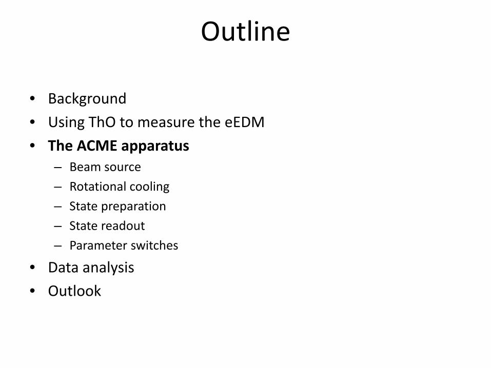
• Background• Using ThO to measure the eEDM• The ACME apparatus• Data analysis• Outlook

Outline

• Background– What is an EDM?– Why is the electron’s EDM small?– Why are we trying to measure it anyway?– How are we trying to do that?

• Using ThO to measure the eEDM• The ACME apparatus• Data analysis• Outlook

Electromagnetic moments of the electron• The electron has spin 𝑆𝑆 = 1/2.• Can specify one axis (plus

overall phase)– Bloch sphere representation

• Allows for only monopole, dipole moments– E.g., quadrupole has two axes

• Dipole parallel to spin axis: 𝑑𝑑 ∝𝑆𝑆

Known and forbidden moments• Electric monopole (charge):

𝐻𝐻𝑞𝑞 =12𝑚𝑚

�⃗�𝑝 − 𝑞𝑞𝐴𝐴2

+ 𝑞𝑞𝑞𝑞

• Magnetic dipole (spin):𝐻𝐻𝜇𝜇 = −�⃗�𝜇 ⋅ 𝐵𝐵

Forbidden:• Magnetic monopole• Toroidal moments (e.g., “anapole moment”)• All higher-order moments (quadrupole, octupole, etc.)

𝐻𝐻𝑑𝑑 = −2𝑑𝑑𝑆𝑆 ⋅ 𝐸𝐸

Symmetry transformations:

• 𝑇𝑇: 𝑆𝑆 → −𝑆𝑆• 𝑇𝑇:𝐸𝐸 → 𝐸𝐸• 𝑃𝑃: 𝑆𝑆 → 𝑆𝑆• 𝑃𝑃:𝐸𝐸 → −𝐸𝐸

So:

𝑇𝑇:𝐻𝐻𝑑𝑑 → −𝐻𝐻𝑑𝑑𝑃𝑃:𝐻𝐻𝑑𝑑 → −𝐻𝐻𝑑𝑑

Why is the electric dipole moment small*?

+++++++

-------S

E

+++++++

-------S

E

-------

+++++++S

E

T

P

𝐻𝐻𝑑𝑑 = +|𝑑𝑑𝐸𝐸|

𝐻𝐻𝑑𝑑,𝑃𝑃 = −|𝑑𝑑𝐸𝐸|

𝐻𝐻𝑑𝑑,𝑇𝑇 = −|𝑑𝑑𝐸𝐸|

*I will say “small compared to what” shortly

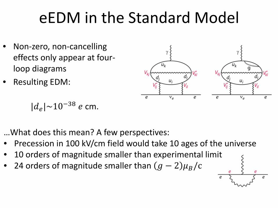
eEDM in the Standard Model• Non-zero, non-cancelling

effects only appear at four-loop diagrams

• Resulting EDM:

|𝑑𝑑𝑒𝑒|~10−38 𝑒𝑒 cm.

…What does this mean? A few perspectives:• Precession in 100 kV/cm field would take 10 ages of the universe• 10 orders of magnitude smaller than experimental limit• 24 orders of magnitude smaller than 𝑔𝑔 − 2 𝜇𝜇𝐵𝐵/c

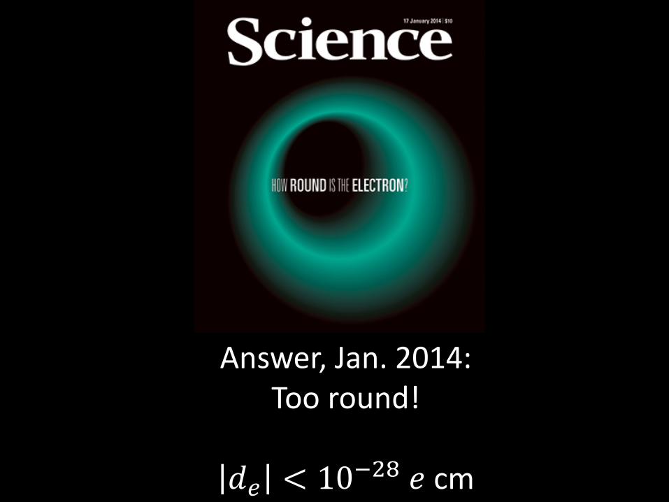
Answer, Jan. 2014:Too round!

𝑑𝑑𝑒𝑒 < 10−28 𝑒𝑒 cm

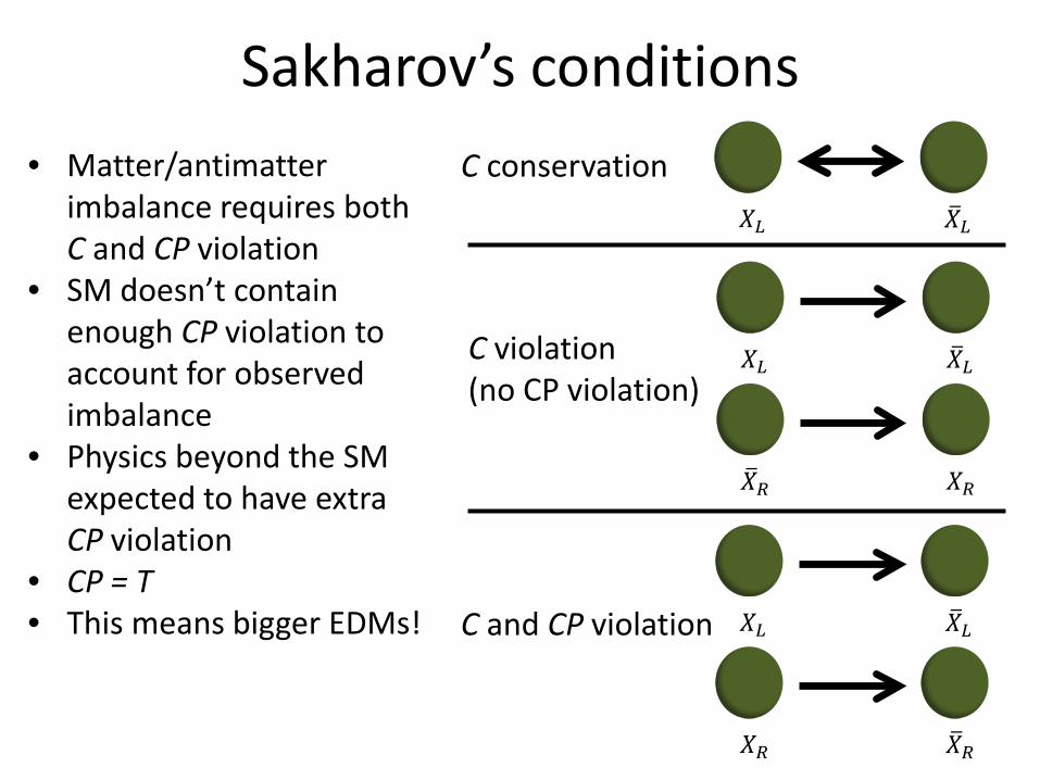
Sakharov’s conditions

𝑋𝑋𝐿𝐿 �𝑋𝑋𝐿𝐿C violation(no CP violation)

�𝑋𝑋𝑅𝑅 𝑋𝑋𝑅𝑅

𝑋𝑋𝐿𝐿 �𝑋𝑋𝐿𝐿

C conservation

𝑋𝑋𝐿𝐿 �𝑋𝑋𝐿𝐿C and CP violation

𝑋𝑋𝑅𝑅 �𝑋𝑋𝑅𝑅

• Matter/antimatter imbalance requires both C and CP violation

• SM doesn’t contain enough CP violation to account for observed imbalance

• Physics beyond the SM expected to have extra CP violation

• CP = T• This means bigger EDMs!

eEDM beyond the Standard Model

With a new particle X and CP-violating phase 𝑞𝑞, a (𝑔𝑔 − 2)-type Feynman diagram (above) gives:

(assuming natural units with 𝑓𝑓~𝑒𝑒 and 𝑞𝑞~1)With 𝑚𝑚𝑋𝑋~10 TeV, obtain 𝑑𝑑𝑒𝑒~5 × 10−29𝑒𝑒 cm.

Outline

• Background• Using ThO to measure the eEDM

– Relativistic enhancement– Benefits of the Ω doublet and 3Δ1 structure– Other benefits of ThO

• The ACME apparatus• Data analysis• Outlook

EDM measurement scheme𝐻𝐻 = −𝜇𝜇 ⋅ 𝐵𝐵 − 𝑑𝑑 ⋅ 𝐸𝐸

Time 𝜏𝜏

Figure of merit: 1Δ𝑑𝑑

∝ 𝐸𝐸𝜏𝜏 �̇�𝑁𝑇𝑇

𝐵𝐵 𝐸𝐸

𝑞𝑞+ = 𝜇𝜇𝐵𝐵𝜏𝜏 + 𝑑𝑑𝐸𝐸𝜏𝜏

Time 𝜏𝜏

𝐵𝐵 𝐸𝐸

𝑞𝑞− = 𝜇𝜇𝐵𝐵𝜏𝜏 − 𝑑𝑑𝐸𝐸𝜏𝜏

𝑑𝑑 ∝ 𝑞𝑞+ − 𝑞𝑞−

𝐸𝐸 = electric field𝜏𝜏 = precession time�̇�𝑁 = experiment repetition rate𝑇𝑇 = integration time

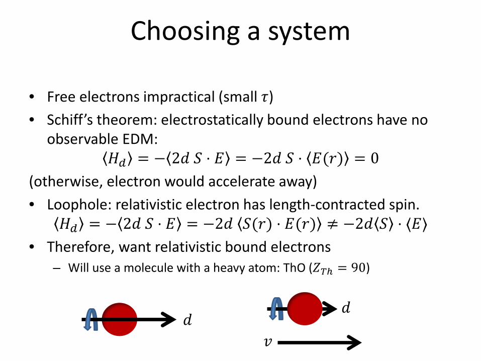
• Free electrons impractical (small 𝜏𝜏)• Schiff’s theorem: electrostatically bound electrons have no

observable EDM:𝐻𝐻𝑑𝑑 = − 2𝑑𝑑 𝑆𝑆 ⋅ 𝐸𝐸 = −2𝑑𝑑 𝑆𝑆 ⋅ 𝐸𝐸(𝑟𝑟) = 0

(otherwise, electron would accelerate away)• Loophole: relativistic electron has length-contracted spin.

𝐻𝐻𝑑𝑑 = − 2𝑑𝑑 𝑆𝑆 ⋅ 𝐸𝐸 = −2𝑑𝑑 𝑆𝑆(𝑟𝑟) ⋅ 𝐸𝐸(𝑟𝑟) ≠ −2𝑑𝑑 𝑆𝑆 ⋅ ⟨𝐸𝐸⟩• Therefore, want relativistic bound electrons

– Will use a molecule with a heavy atom: ThO (𝑍𝑍𝑇𝑇𝑇 = 90)

Choosing a system

𝑑𝑑𝑣𝑣

𝑑𝑑

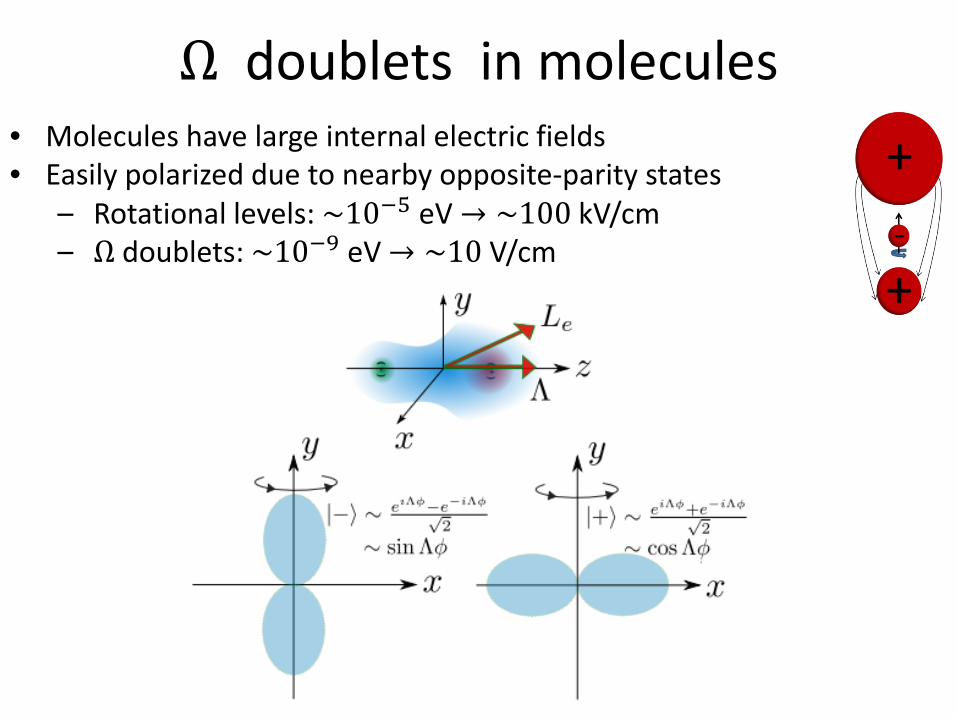
Ω doublets in molecules• Molecules have large internal electric fields• Easily polarized due to nearby opposite-parity states

– Rotational levels: ~10−5 eV → ~100 kV/cm– Ω doublets: ~10−9 eV → ~10 V/cm

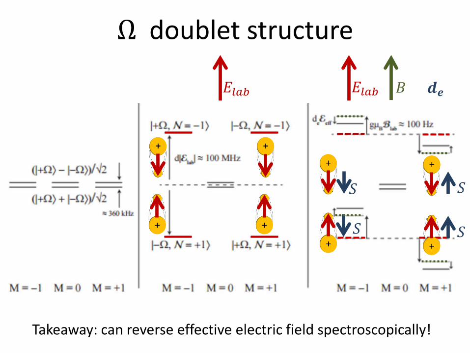
Ω doublet structure

𝐵𝐵𝐸𝐸𝑙𝑙𝑙𝑙𝑙𝑙 𝐸𝐸𝑙𝑙𝑙𝑙𝑙𝑙

𝑆𝑆 𝑆𝑆

𝑆𝑆 𝑆𝑆

𝒅𝒅𝒆𝒆

Takeaway: can reverse effective electric field spectroscopically!

3Δ1 structure

Choose a state with:• |𝑆𝑆𝑧𝑧| = 1• |𝐿𝐿𝑧𝑧| = 2• �̂�𝑆 = −�𝐿𝐿→ |𝜇𝜇𝑡𝑡𝑡𝑡𝑡𝑡| = |𝑔𝑔𝑠𝑠𝑆𝑆𝑧𝑧 + 𝑔𝑔𝐿𝐿𝐿𝐿𝑧𝑧|𝜇𝜇𝐵𝐵

≈ 2 × 1 + 1 × −2 𝜇𝜇𝐵𝐵= 0.

(Actually, 𝑔𝑔𝑡𝑡𝑡𝑡𝑡𝑡 ≈ 10−2.)

+

+

-|𝑆𝑆| = 1

|𝐿𝐿| = 2

Criteria favorable to ThO• Large effective electric field (relativistic; heavy nucleus)• Polarizable (omega doublet)• Orientations in applied field spectroscopically resolvable

• Diatomic (simple spectra)• Transitions accessible by lasers• Spectroscopy worked out before our experiment

• Magnetically insensitive (systematic error rejection)• “Long” lifetime (precession time) in science state: ~1 ms

• Efficiently produced in a beam

Outline

• Background• Using ThO to measure the eEDM• The ACME apparatus

– Beam source– Rotational cooling– State preparation– State readout– Parameter switches

• Data analysis• Outlook

Doing the measurement

1. Create a molecular beam2. Consolidate to a single quantum state3. Transfer to the 3Δ1 science state4. Polarize the molecule5. Orient the spin6. Wait for precession7. Read out the spin precession

12

3-5 6 7

Doing the measurement

𝑋𝑋 𝐽𝐽 = 0,1,2,3 → 𝑋𝑋 𝐽𝐽 = 0𝑋𝑋 𝐽𝐽 = 0 → 𝐻𝐻 𝐽𝐽 = 1 (|+⟩ + |−⟩)

|+⟩ + 𝑒𝑒𝑖𝑖𝑖𝑖𝑖𝑖|−⟩

H

X

I�𝑥𝑥, �𝑦𝑦

cos 𝜔𝜔𝜏𝜏 ∝ 𝑆𝑆𝑦𝑦 − 𝑆𝑆𝑥𝑥

…and actually doing the measurement

Closer look: beam source

𝑋𝑋 𝐽𝐽 = 0,1,2,3 → 𝑋𝑋 𝐽𝐽 = 0𝑋𝑋 𝐽𝐽 = 0 → 𝐻𝐻 𝐽𝐽 = 1 (|+⟩ + |−⟩)

|+⟩ + 𝑒𝑒𝑖𝑖𝑖𝑖𝑖𝑖|−⟩

H

X

I�𝑥𝑥, �𝑦𝑦

cos 𝜔𝜔𝜏𝜏 ∝ 𝑆𝑆𝑦𝑦 − 𝑆𝑆𝑥𝑥

Beam source: laser ablation

• ThO2 ablated by pulsed Nd:YAG laser• Some of the ablation plume is ThO• The plume is entrained in a flow of cold neon buffer gas

• Slow (180 m/s)• Cold (~all ThO molecules in vibronic ground state, 𝑇𝑇𝑟𝑟𝑡𝑡𝑡𝑡~4 K)• Relatively high flux. ThO ablation source: 5 × 1012 mol/sec

Buffer-gas beam source

Thermochemical source● Drive reaction by heating:

● Use 10 W fiber laser

● 10x higher flux!

● Radioactive dust high

● Target lifetimes low

Closer look: Optical pumping

𝑋𝑋 𝐽𝐽 = 0,1,2,3 → 𝑋𝑋 𝐽𝐽 = 0𝑋𝑋 𝐽𝐽 = 0 → 𝐻𝐻 𝐽𝐽 = 1 (|+⟩ + |−⟩)

|+⟩ + 𝑒𝑒𝑖𝑖𝑖𝑖𝑖𝑖|−⟩

H

X

I�𝑥𝑥, �𝑦𝑦

cos 𝜔𝜔𝜏𝜏 ∝ 𝑆𝑆𝑦𝑦 − 𝑆𝑆𝑥𝑥

Rotational cooling

• Rotational temperature ~4 K• Drive population to 𝐽𝐽 = 0• Increase population by ~ 4x• No gain relative to Gen. I

Closer look: STIRAP

𝑋𝑋 𝐽𝐽 = 0,1,2,3 → 𝑋𝑋 𝐽𝐽 = 0𝑋𝑋 𝐽𝐽 = 0 → 𝐻𝐻 𝐽𝐽 = 1 (|+⟩ + |−⟩)

|+⟩ + 𝑒𝑒𝑖𝑖𝑖𝑖𝑖𝑖|−⟩

H

X

I�𝑥𝑥, �𝑦𝑦

cos 𝜔𝜔𝜏𝜏 ∝ 𝑆𝑆𝑦𝑦 − 𝑆𝑆𝑥𝑥

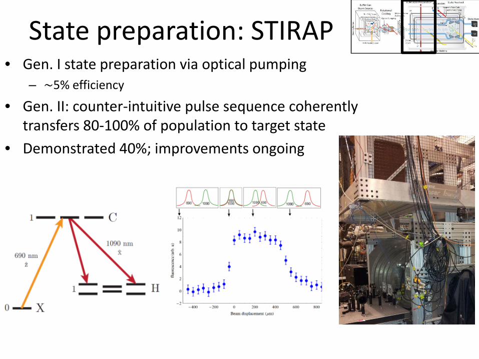
• Gen. I state preparation via optical pumping– ~5% efficiency

• Gen. II: counter-intuitive pulse sequence coherently transfers 80-100% of population to target state

• Demonstrated 40%; improvements ongoing

State preparation: STIRAP

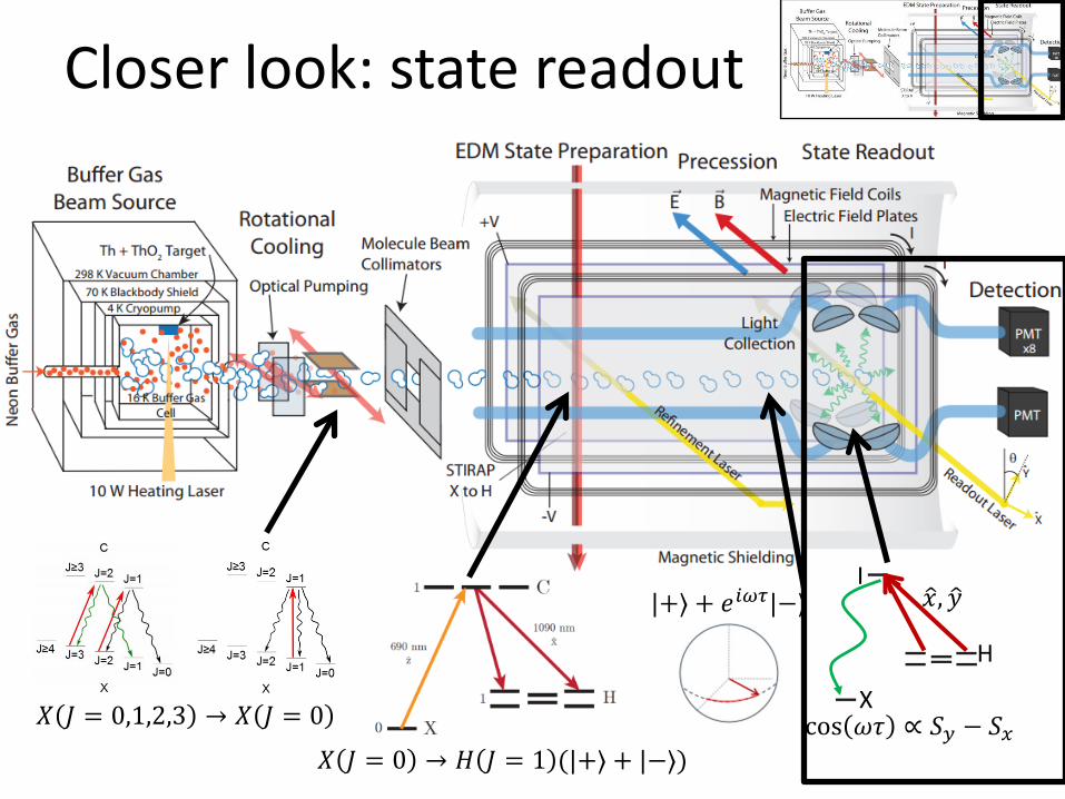
Closer look: state readout

𝑋𝑋 𝐽𝐽 = 0,1,2,3 → 𝑋𝑋 𝐽𝐽 = 0𝑋𝑋 𝐽𝐽 = 0 → 𝐻𝐻 𝐽𝐽 = 1 (|+⟩ + |−⟩)

|+⟩ + 𝑒𝑒𝑖𝑖𝑖𝑖𝑖𝑖|−⟩

H

X

I�𝑥𝑥, �𝑦𝑦

cos 𝜔𝜔𝜏𝜏 ∝ 𝑆𝑆𝑦𝑦 − 𝑆𝑆𝑥𝑥

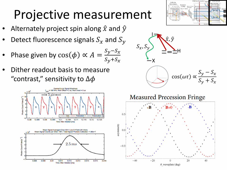
Projective measurement• Alternately project spin along �𝑥𝑥 and �𝑦𝑦• Detect fluorescence signals 𝑆𝑆𝑥𝑥 and 𝑆𝑆𝑦𝑦

• Phase given by cos 𝑞𝑞 ∝ 𝐴𝐴 = 𝑆𝑆𝑦𝑦−𝑆𝑆𝑥𝑥𝑆𝑆𝑦𝑦+𝑆𝑆𝑥𝑥

• Dither readout basis to measure “contrast,” sensitivity to Δ𝑞𝑞 cos 𝜔𝜔𝜏𝜏 ∝

𝑆𝑆𝑦𝑦 − 𝑆𝑆𝑥𝑥𝑆𝑆𝑦𝑦 + 𝑆𝑆𝑥𝑥

H

X

I�𝑥𝑥, �𝑦𝑦

𝑆𝑆𝑥𝑥 , 𝑆𝑆𝑦𝑦

Fluorescence collection

• Collect 512 nm fluorescence using lenses and light pipes– 10-20% photon collection efficiency

• Quantum efficiency with photomultiplier tubes: 20-25%– Overall efficiency: 2-5%

• Very preliminary: switch to silicon photomultipliers? (QE ~40%)

Repeat under different conditions• 1 min: A “block” of data contains all

switches for an independent “EDM experiment”

• 30 mins: A “superblock” contains auxiliary switches for systematic checks

• 1 hr: The magnetic field magnitude is varied across superblocks

• 5 hrs: Some superblocks are performed with parameters intentionally varied (IPV)

• 1 day: The electric field magnitude is changed between “runs”

• 1 wk: The propagation direction of lasers for state preparation and readout is reversed

• 2 wks: All data for the Jan. 2014 result

Before this: 1 year of systematic checks!

Outline

• Background• Using ThO to measure the eEDM• The ACME apparatus• Data analysis

– Extracting the eEDM– Checking for systematic errors

• Outlook

Extracting the eEDMDecompose phase according to parity under experimental switches:

𝑞𝑞 = 𝑞𝑞0 + 𝑞𝑞𝑁𝑁 + 𝑞𝑞𝐸𝐸 + 𝑞𝑞𝐵𝐵 + 𝑞𝑞𝑁𝑁𝐸𝐸 + 𝑞𝑞𝑁𝑁𝐵𝐵 + 𝑞𝑞𝐸𝐸𝐵𝐵 + 𝑞𝑞𝑁𝑁𝐸𝐸𝐵𝐵

𝑁𝑁 = �𝐸𝐸𝑚𝑚𝑡𝑡𝑙𝑙 ⋅ �𝐸𝐸𝑙𝑙𝑙𝑙𝑙𝑙𝐸𝐸 = �𝐸𝐸𝑙𝑙𝑙𝑙𝑙𝑙 ⋅ �̂�𝑧𝐵𝐵 = �𝐵𝐵𝑙𝑙𝑙𝑙𝑙𝑙 ⋅ �̂�𝑧

EDM here! (Or not.)• Reverses with 𝑁𝑁 and 𝐸𝐸• Doesn’t reverse with 𝐵𝐵

𝑞𝑞𝑁𝑁𝐸𝐸 = 2(𝑑𝑑𝐸𝐸𝑚𝑚𝑡𝑡𝑙𝑙)𝜏𝜏 + 𝑞𝑞𝑠𝑠𝑦𝑦𝑠𝑠𝑡𝑡𝑁𝑁𝐸𝐸

Many other terms in the Hamiltonian…

Non-EDM channels used to understand systematic errors

Checking for systematic errors1. Exaggerate parameter variation2. Check effect on 𝑞𝑞𝑁𝑁𝐸𝐸

3. Measure normal parameter variation4. Infer normal effect on 𝑞𝑞𝑁𝑁𝐸𝐸

• Repeat for many parameters…– Laser detuning, power, pointing, polarization– Field plate voltage offset– Molecular beam shape (via clipping)– Magnetic field gradients– Non-reversing electric and magnetic field– Polarization switching rate

• In analysis, vary:– Data cut thresholds, time within molecular pulse profile, correlations

with auxiliary parameters like vacuum pressure, time over dataset…

Outline

• Background• Using ThO to measure the eEDM• The ACME apparatus• Data analysis• Outlook

Outlook• Gen. I:

– good Gaussian statistics– Found Δ𝑑𝑑𝑠𝑠𝑦𝑦𝑠𝑠𝑡𝑡 < Δ𝑑𝑑𝑠𝑠𝑡𝑡𝑙𝑙𝑡𝑡

• Gen. II statistical improvements (250-500x):– State preparation: 8x (16x?)– Fluorescence collection in light pipes: 2x– Detection at 512 nm: 2x– Beam solid angle: 8x

• Gen. III improvements (with above, >104x):– Thermochemical beam source: 10x?– Detection with silicon photomultipliers: 2x?– Electrostatic lens: 3x?– Optical cycling: 6x??

Projected Gen. II improvements

10x8x

8x-16x 2x 2xThermochemical

beam source

Solidangle

STIRAP statepreparation

Fluorescencecollection

PMTs@512 nm

What could go wrong?

Systematics not expected to be limiting…but needs to be thoroughly checked

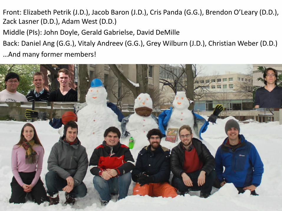
Front: Elizabeth Petrik (J.D.), Jacob Baron (J.D.), Cris Panda (G.G.), Brendon O’Leary (D.D.), Zack Lasner (D.D.), Adam West (D.D.)Middle (PIs): John Doyle, Gerald Gabrielse, David DeMilleBack: Daniel Ang (G.G.), Vitaly Andreev (G.G.), Grey Wilburn (J.D.), Christian Weber (D.D.)…And many former members!

Questions?

Extra slides

How STIRAP works• Foolproof method:

1. Write down Hamiltonian. 2. Diagonalize.3. Look at answer.

• More intuitive example:1. Imagine |1⟩ and |2⟩ have

orthogonal spin projections; each couples to only one laser polarization, �𝑥𝑥 or �𝑦𝑦. Population initially in |1⟩.

2. Turn on laser driving 2 ↔ 3 .3. Slowly rotate polarization.

Population stays in “dark” state (adiabatic theorem).

4. Once polarization is rotated, the “dark” state is 2 .

5. Ramp down laser.

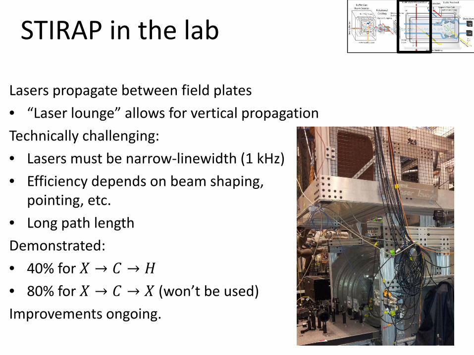
STIRAP in the lab

Lasers propagate between field plates• “Laser lounge” allows for vertical propagationTechnically challenging:• Lasers must be narrow-linewidth (1 kHz)• Efficiency depends on beam shaping,

pointing, etc.• Long path lengthDemonstrated:• 40% for 𝑋𝑋 → 𝐶𝐶 → 𝐻𝐻• 80% for 𝑋𝑋 → 𝐶𝐶 → 𝑋𝑋 (won’t be used)Improvements ongoing.

Forbidden electromagnetic moments

• Magnetic monopole: 𝛻𝛻 ⋅ 𝐵𝐵 = 0• Toroidal monopole: (Static limit) 𝛻𝛻 ⋅ 𝐽𝐽 = 0• Toroidal dipole: Not invariant under

electroweak gauge transformations; not physically meaningful in SM.

• Quadrupole, octupole, etc.: 𝑆𝑆 = 1/2 for the electron