improving simulation of biological molecules:...
TRANSCRIPT

Improving simulationof biological molecules:
refining mathematical, physical andcomputational tools
Pablo García RisueñoDepartamento de Física Teórica, Universidad de
ZaragozaInstituto de Química Física Rocasolano, CSIC


Table of Contents
Aknowledgements i
Resumen (en Español) iii
Summary (in English) vii
1 Aim and scope 1
2 Physical basis 52.1 Quantum Mechanics . . . . . . . . . . . . . . . . . . . . . . . . . . . . 52.2 Density Functional Theory . . . . . . . . . . . . . . . . . . . . . . . . . 102.3 Time-Dependent Density Functional Theory . . . . . . . . . . . . . . . . 272.4 Lower level methods . . . . . . . . . . . . . . . . . . . . . . . . . . . . 302.5 Calculating observable quantities . . . . . . . . . . . . . . . . . . . . . . 34
3 Computational aspects 393.1 Running algorithms in real computers . . . . . . . . . . . . . . . . . . . 393.2 Scientific supercomputing . . . . . . . . . . . . . . . . . . . . . . . . . 43
3.2.1 Introduction . . . . . . . . . . . . . . . . . . . . . . . . . . . . . 433.2.2 Hardware basics . . . . . . . . . . . . . . . . . . . . . . . . . . 443.2.3 Beyond the Von Neumann paradigm . . . . . . . . . . . . . . . . 463.2.4 Parallel computers . . . . . . . . . . . . . . . . . . . . . . . . . 503.2.5 Hybrid and heterogeneous models . . . . . . . . . . . . . . . . . 573.2.6 Distributed computing . . . . . . . . . . . . . . . . . . . . . . . 62
4 Classical potential solvers 654.1 Introduction . . . . . . . . . . . . . . . . . . . . . . . . . . . . . . . . . 654.2 Methods . . . . . . . . . . . . . . . . . . . . . . . . . . . . . . . . . . . 66
4.2.1 Parallel Fast Fourier Transform . . . . . . . . . . . . . . . . . . 674.2.2 Interpolating Scaling Functions . . . . . . . . . . . . . . . . . . 694.2.3 Fast Multipole Method . . . . . . . . . . . . . . . . . . . . . . . 704.2.4 Multigrid . . . . . . . . . . . . . . . . . . . . . . . . . . . . . . 734.2.5 Conjugate gradients . . . . . . . . . . . . . . . . . . . . . . . . 73
4.3 Results . . . . . . . . . . . . . . . . . . . . . . . . . . . . . . . . . . . . 744.4 Conclusions . . . . . . . . . . . . . . . . . . . . . . . . . . . . . . . . . 75
TABLE OF CONTENTS
5 Excited States of the Green Fluorescent Protein 815.1 Introduction . . . . . . . . . . . . . . . . . . . . . . . . . . . . . . . . . 815.2 Computational Details . . . . . . . . . . . . . . . . . . . . . . . . . . . 825.3 Results and Discussion . . . . . . . . . . . . . . . . . . . . . . . . . . . 84
5.3.1 Proton Affinities . . . . . . . . . . . . . . . . . . . . . . . . . . 845.3.2 Excitation Energies . . . . . . . . . . . . . . . . . . . . . . . . . 855.3.3 QM/MM on a Real-Space Grid . . . . . . . . . . . . . . . . . . . 89
5.4 Conclusions . . . . . . . . . . . . . . . . . . . . . . . . . . . . . . . . . 91
6 Flexible derivatives 956.1 Introduction . . . . . . . . . . . . . . . . . . . . . . . . . . . . . . . . . 956.2 Methods . . . . . . . . . . . . . . . . . . . . . . . . . . . . . . . . . . . 98
6.2.1 General Algorithm . . . . . . . . . . . . . . . . . . . . . . . . . 986.2.2 Application to Euclidean coordinates of Molecules . . . . . . . . 102
6.3 Results and Discussion . . . . . . . . . . . . . . . . . . . . . . . . . . . 110
7 Equilibrium of constrained molecular models 1197.1 Introduction . . . . . . . . . . . . . . . . . . . . . . . . . . . . . . . . . 1197.2 Theoretical framework and relation to previous works . . . . . . . . . . . 121
7.2.1 Notation . . . . . . . . . . . . . . . . . . . . . . . . . . . . . . 1227.2.2 Hamiltonian dynamics and Statistical Mechanics without constraints1257.2.3 Types of constraints . . . . . . . . . . . . . . . . . . . . . . . . 1297.2.4 Statistical Mechanics models . . . . . . . . . . . . . . . . . . . . 1387.2.5 Summary, comparisons and the Fixman’s potential . . . . . . . . 155
7.3 Numerical examples . . . . . . . . . . . . . . . . . . . . . . . . . . . . 1627.4 Conclusions and future lines of research . . . . . . . . . . . . . . . . . . 167
8 Efficient inversion of banded matrices 1698.1 Introduction . . . . . . . . . . . . . . . . . . . . . . . . . . . . . . . . . 1698.2 Analytical solution of banded systems . . . . . . . . . . . . . . . . . . . 1708.3 Banded plus sparse systems . . . . . . . . . . . . . . . . . . . . . . . . . 1798.4 Algorithmic implementation . . . . . . . . . . . . . . . . . . . . . . . . 1808.5 Parallelization . . . . . . . . . . . . . . . . . . . . . . . . . . . . . . . . 1838.6 Differences with Gaussian elimination . . . . . . . . . . . . . . . . . . . 1838.7 Numerical tests . . . . . . . . . . . . . . . . . . . . . . . . . . . . . . . 186
8.7.1 Performance for generic random banded systems . . . . . . . . . 1868.7.2 Analytical calculation of Lagrange multipliers in a protein . . . . 189
8.8 Concluding remarks . . . . . . . . . . . . . . . . . . . . . . . . . . . . . 192
9 Lagrange multipliers in biological polymers 1939.1 Introduction . . . . . . . . . . . . . . . . . . . . . . . . . . . . . . . . . 1939.2 Calculation of the Lagrange multipliers . . . . . . . . . . . . . . . . . . 1969.3 Smart ordering of constraints . . . . . . . . . . . . . . . . . . . . . . . . 201
9.3.1 Open, single-branch chain with constrained bond lengths . . . . . 2029.3.2 Open, single-branch chain with constrained bond lengths and bond
angles . . . . . . . . . . . . . . . . . . . . . . . . . . . . . . . . 2039.3.3 Minimally branched molecules with constrained bond lengths . . 204
TABLE OF CONTENTS
9.3.4 Alkanes with constrained bond lengths . . . . . . . . . . . . . . 2049.3.5 Minimally branched molecules with constrained bond lengths and
bond angles . . . . . . . . . . . . . . . . . . . . . . . . . . . . . 2059.3.6 Alkanes with constrained bond lengths and bond angles . . . . . 2059.3.7 Cyclic chains . . . . . . . . . . . . . . . . . . . . . . . . . . . . 2069.3.8 Proteins . . . . . . . . . . . . . . . . . . . . . . . . . . . . . . . 2079.3.9 Nucleic acids . . . . . . . . . . . . . . . . . . . . . . . . . . . . 209
9.4 Numerical calculations . . . . . . . . . . . . . . . . . . . . . . . . . . . 2119.5 Conclusions . . . . . . . . . . . . . . . . . . . . . . . . . . . . . . . . . 215
Appendices 219A Corrections for the Fast Multipole Method in a grid . . . . . . . . . . . . . 219
Method 1: 6-neighbours correction . . . . . . . . . . . . . . . . . . . . . 221Method 2: 124-neighbours correction . . . . . . . . . . . . . . . . . . . 223
B Supplementary information for chapter 5 . . . . . . . . . . . . . . . . . . 227Basis Set Convergence . . . . . . . . . . . . . . . . . . . . . . . . . . . 227Generalized Bond Length Alternation . . . . . . . . . . . . . . . . . . . 227TDDFT Time-Propagation Spectra . . . . . . . . . . . . . . . . . . . . . 228
C Explicit inversion of a sparse banded matrix . . . . . . . . . . . . . . . . . 229D Efficient calculation of derivatives of Lagrange multipliers into Robotics . . 232
Introduction . . . . . . . . . . . . . . . . . . . . . . . . . . . . . . . . . 232Analysing a hexapod-shaped parallel manipulator . . . . . . . . . . . . . 232Exact calculation of derivatives of Lagrange multipliers . . . . . . . . . . 241
Acronyms 245
Bibliography 247
Index 275


Aknowledgements
To my thesis directors, José Luis Alonso, Pablo Echenique and Ángel Rubio.
To all the people who enjoy Science, and work for a better world.
A special dedication for all the people who has helped me during these years.


Resumen
El objetivo de las investigaciones correspondientes a este documento de tesis doctorales la mejora de los métodos para la simulación de moléculas, especialmente moléculasbiológicas, como las proteínas. Las capacidades de los ordenadores han aumentado so-bremanera en las últimas décadas, y actualmente son una herramienta poderosa para elcálculo de magnitudes físicas y químicas. Debido a esto, un gran número de investi-gadores se dedica al desarrollo de métodos computacionales precisos y eficientes, a suuso en simulaciones con fines científicos, a una mezcla de ambos o a otros campos dentrode la ciencia computacional. El trabajo de investigación resumido en esta tesis tiene comofinalidad la mejora de la eficiencia y exactitud de los métodos de simulación de moléculasbiológicas.
Podemos resumir la estructura de esta tesis como sigue:
• En el capítulo 1, titulado “Aim and scope”, se efectúa un breve repaso al campo dela simulación molecular. Los objetivos de esta tesis se explican en la parte final deeste capítulo.
Los capítulos del 2 y 3 son introductorios, al contrario que los capítulos 4 al 9, que estánbasados en trabajos de investigación. Estos capítulos introductorios presentan algunosconceptos fundamentales en que se sustentan los trabajos de investigación.
• El segundo capítulo, titulado “Physical basis”, resume algunos fundamentos de laFísica en que se basan simulaciones moleculares más habituales. Este capítulo sedivide en cinco secciones. Las tres primeras están dedicadas a explicar algunospuntos básicos de la Mecánica Cuántica, en la que se basan muchas simulacionesmoleculares, por describir esta rama de la Física de forma precisa fenómenos queocurren a pequeña escala y que condicionan buena parte del comportamiento molec-ular. En la primera sección, titulada “The basic quantum equations”, presentamosalgunas ecuaciones básicas de la Física Cuántica. Comenzamos por la ecuación deDirac, que por incluir efectos relativistas y campos magnéticos da una descripciónprecisa del comportamiento de los electrones, que a su vez condicionan grande-mente el comportamiento molecular. A continuación, comentamos brevemente lasecuaciones de Pauli y de Schrödinger, que pueden obtenerse de la ecuación de Diracmediante ciertas aproximaciones. En la segunda sección de este segundo capítuloexplicamos algunas nociones básicas de la Teoría del Funcional de Densidad (DFT).Este nivel de teoría es útil para calcular magnitudes físicas de sistemas que se en-cuentran en su estado fundamental. En la sección 2.3 explicamos la Teoría delFuncional de Densidad Dependiente del Tiempo (TDDFT), que puede usarse paracalcular estados excitados de moléculas y algunas de sus propiedades ópticas. Parte

iv RESUMEN
de los cálculos del capítulo 5 están basados en TDDFT, y parte del trabajo pre-sentado en el capítulo 4 consistió en la implementación de nuevos algoritmos enun código (Octopus, [6]) de simulación basada en DFT y TDDFT. La cuarta sec-ción del capítulo 2 explica los fundamentos de métodos de simulación molecularde un nivel más bajo que el de los explicados anteriormente, como son los métodossemiempíricos, la Mecánica Molecular o esquemas mixtos entre Mecánica Cuán-tica y Mecánica Molecular. Finalmente, en la última sección del capítulo 2 (sección2.5) se explican métodos para el cálculo de magnitudes en sistemas moleculares,como son los métodos de Monte Carlo y la Dinámica Molecular.
• El capítulo 3 (“Computational aspects”) explica nociones básicas sobre computación.Esta sección aparece para dar al lector una exposición más amplia del contexto de lasimulación molecular, que está basada en modelos físicos y químicos, pero requiereconocimientos técnicos para la realización práctica de los cálculos. La sección 3.1,titulada “Running algorithms in real computers”, se explican algunos particularessobre el funcionamiento de los ordenadores que pueden afectar a la exactitud y efi-ciencia de cualquier simulación. En la sección 3.2 (“Scientific supercomputing”),explicamos algunos fundamentos acerca de la computación de alto rendimiento.Primero (en la sección “Hardware basics”) explicamos el funcionamiento de un or-denador estándar, para comentar a continuación (en la sección “Beyond the VonNeumann paradigm”) algunas características de los ordenadores más modernos.Después de presentar estos fundamentos, explicamos algunos aspectos de la com-putación de alto rendimiento en sí. En la sección “Parallel computers” se explicandos paradigmas de arquitectura de supercomputadores, los modelos de máquinas dememoria compartida y de memoria distribuída. En la sección “Hybrid an heteroge-neous models” comentamos brevemente otros patrones de arquitectura. Finalmente,en la sección “Distributed computing” se dan algunas nociones sobre métodos decomputación basados en el uso de recursos geográficamente distantes, como la com-putación en grid o en la nube.
Los capítulos 4 al 9 presentan trabajos de investigación encaminados a la mejora de lastécnicas de simulación de moléculas biológicas. Los capítulos 4 y 5 están parcialmentebasados en DFT y TDDFT.
• El capítulo 4 es un estudio de diferentes métodos para calcular el potencial elec-trostático creado por una distribución de carga representada en una red en el es-pacio real. Para tales sistemas, comparamos la exactitud y eficiencia de diferentesmétodos para calcular dicho potencial. Una parte significativa del trabajo resumidoen este capítulo consistió en la implementación de dos métodos populares y moder-nos (la tranformada de Fourier rápida en paralelo y una versión reciente del métodomultipolar rápido) en el código Octopus [6], un programa de simulación basada enDFT y TDDFT.
• El capítulo 5 está basado en el artículo Excited States of the Green Fluorescent Pro-tein Chromophore: Performance of Ab Initio and Semi-Empirical Methods, escritopor M. Wanko, P. García-Risueño and Á. Rubio, y aceptado por Physica Status So-lidi en 2011. Este capítulo es un análisis del rendimiento de diferentes métodos parael cálculo del espectro de absorción óptica de la proteína fluorescente verde. Esta

RESUMEN v
proteína tiene significativas aplicaciones en bioquímica y fisiología, lo que la ha he-cho objeto de numerosos estudios teóricos. En este capítulo se usan varios nivelesde teoría diferentes, como métodos semiempíricos, QM/MM, DFT y TDDFT.
Los capítulos 6 al 9 versan sobre cálculos de magnitudes en sistemas sujetos a ligaduras.Las ligaduras se imponen a los modelos de sistemas moleculares para aumentar la eficien-cia de algunos cálculos, tanto en Dinámica Molecular como en Mecánica Estadística.
• El capítulo 6 se titula “An Exact Expression to Calculate the Derivatives of Position-Dependent Observables in Molecular Simulations with Flexible Constraints”, y estábasado en el artículo del mismo nombre escrito por P. Echenique, C. N. Cavasotto,M. De Marco, P. García-Risueño y J. L. Alonso publicado en PloS One 6(9): (2011)e24563. Cuando se imponen ligaduras (constraints) a un sistema, éstas puedenser flexibles o no flexibles. Las primeras permiten mayor libertad a los sistemas,y por tanto dan lugar (en principio) a descripciones más exactas. Las derivadasde magnitudes que dependen de las posiciones de un sistema molecular puedenser calculadas por diferencias finitas, pero esto da lugar a errores, puesto que elvalor de la derivada depende de la distancia entre los puntos elegidos para hacerlas diferencias finitas. El nuevo algoritmo presentado en este capítulo resuelve esteproblema, calculando el valor exacto del tipo de derivadas que nos ocupa.
• El capítulo 7 se titula “The canonical equilibrium of constrained models”, y estábasado en el artículo homónimo escrito por P. Echenique, C. N. Cavasotto y P.García-Risueño, y aceptado en 2011 por el European Physics Journal. En este capí-tulo se explican los modelos stiff y rígido de la Mecánica Estadística para los casosde ligaduras flexibles y no flexibles. Estos diferentes modelos tienen complejidadesdiferentes, y en principio también precisiones diferentes. A modo de ejemplo, eneste capítulo se incluyen cálculos de los diferentes términos de la energía libre de unsistema sencillo (metanol), para ilustrar las diferencias entre unos modelos y otros.Estos términos son relevantes, porque la energía libre de una conformación dadadetermina el peso de esta conformación en el cálculo de las magnitudes observablescalculadas en el marco de la Mecánica Estadística.
• En el capítulo 8, titulado “Linearly scaling direct method for accurately invertingsparse banded matrices”, se presenta un algoritmo para resolver un sistema linealde ecuaciones Ax = b, con A una matriz de banda N × N. Las matrices de bandason un tipo especial de matrices sparse, en las que todas las entradas no nulas seconcentran en una banda en torno a la diagonal. Estas matrices aparecen en algunosproblemas de Dinámica Molecular ligada, como el del cálculo de multiplicadoresde Lagrange del capítulo 9. Nuestro algoritmo puede resolver el citado sistemalineal de manera analítica, exacta en precisión máquina, y asimismo eficiente, conun scaling de O(N) con un prefactor bajo. Este capítulo se basa en un artículoescrito por P. García-Risueño y P. Echenique, actualmente submitido.
• El capítulo 9, titulado “Exact and efficient calculation of Lagrange multipliers inbiological polymers with constrained bond lengths and bond angles”, explica cómocalcular exactamente los multiplicadores de Lagrange correspondientes a ligaduras

vi RESUMEN
holónomas impuestas en moléculas biológicas. Esto puede hacerse de manera efi-ciente, en O(N) operaciones, siendo N el número de ligaduras impuestas. Esto sedebe a la topología de las moléculas biológicas, como proteínas y ácidos nucle-icos, que es esencialmente lineal. Este capítulo se basa en el artículo escrito por P.García-Risueño, P. Echenique y J. L. Alonso, publicado en J. Comp. Chem. 32, 14(2011) 3039–3046.
Aparte de los artículos nombrados arriba en los que se basa el contenido de esta tesis,tenemos la intención de submitir en breve otros basados en los capítulos 3 y 4.
Tras los capítulos basados en trabajos de investigación incluímos apéndices con in-formación complementaria. En el apéndice A presentamos las fórmulas de dos métodospara incrementar la exactitud del método multipolar rápido usado en el capítulo 4. En elapéndice B incluímos información complementaria al capítulo 5, que incluye datos adi-cionales sobre las bases usadas y los espectros obtenidos en las simulaciones. El apéndiceC es un complemento al capítulo 8, e introduce un algoritmo para calcular explícitamentela inversa de una matriz N × N en O(N2) operaciones. El apéndice D presenta un métodopara calcular de manera precisa y eficiente los multiplicadores de Lagrange de un ma-nipulador paralelo (un tipo de robot) y sus derivadas temporales. Este apéndice es uncomplemento del capítulo 9, y lo incluímos para remarcar la amplitud del campo de apli-cación de los métodos presentados en dicho capítulo.
Finalmente, las últimas tres secciones, que siguen a los apéndices, contienen, respec-tivamente, la lista de acrónimos usados en este documento, la bibliografía de todos loscapítulos y el índice que contiene algunas de las palabras más representativas de estatesis.

Summary
The goal of the research summarized in this Ph. D. dissertation is the improvement of thecomputational methods for simulation of molecules, specially biological molecules suchas proteins. The performance of computers has strongly increased during the last decades,and at present they are a powerful tool for the calculation of physical and chemical quan-tities. Because of this, there exist a large number of researchers who work either as de-velopers of reliable and efficient computational methods to make calculations on physicaland chemical systems, or as users of existing algorithms and programs for scientific pur-poses. The work presented in this dissertation is expected to improve the efficiency andaccuracy of simulations of biological molecules.
The structure of this dissertation can be summarized as follows:
• In chapter 1, entitled “Aim and scope”, a short overview of the field of molecularsimulation is presented. The goal of this dissertation is presented in the last part ofthis chapter.
Chapters 2 and 3 are introductory chapters, while the rest of the chapters (chapters 4 to9) are based on actual research articles such as The introductory chapters present some ofthe fundamental ideas the research the research work of this thesis is based on.
• The second chapter, entitled “Physical basis”, summarizes some fundamentals ofthe Physics behind popular molecular simulations. This chapter is divided into fivesections. We dedicate the first three ones to introducing some fundamentals on cal-culation methods based on Quantum Mechanics, because the physical and chemicalbehaviour of molecules is strongly determined by small scale phenomena which canbe described by Quantum Mechanics. In the first section, which is called “The basicquantum equations”, we present some of its fundamental equations. We start withthe Dirac equation, which includes relativistic corrections and magnetic fields andis very accurate for many calculations on electrons, which have a major influenceon the properties of a molecule. Then, we briefly discuss the equations of Pauliand Schrödinger, which can be derived from the Dirac equation by making someapproximations. In the second section we present the quantum mechanical formal-ism of Density Functional Theory (DFT), which is very useful for the calculationof quantities of systems of molecules whose electrons are lying in its ground statefor given nuclear positions. In section 2.3 we briefly introduce some aspects of theTime-dependent Density Functional Theory (TDDFT) formalism, which is usefulto calculate excited states of molecular systems, as well as some of their opticalproperties. A significant part of the calculations of chapter 5 are based on TDDFT,and part of the work which is presented in chapter 4 was the implementation of

viii SUMMARY
new algorithms in a DFT and TDDFT simulation code (Octopus [6]). The fourthsection of chapter 2 presents some basic ideas about lower level methods to sim-ulate molecules, namely semiempirical methods, Molecular Mechanics and mixedschemes of Quantum Mechanics and Molecular Mechanics (QM/MM). Finally, thelast section of chapter 2 (sec. 2.5) summarizes some methods to calculate observ-able quantities of molecular systems, such as Molecular Dynamics and Monte Carlomethods.
• Chapter 3 (“Computational aspects”) preents some ideas on present day scientificcomputing. We include this section to provide the reader with a complete contextof the field of molecular simulations, which are based on physical and chemicalmodels, but require for its execution the knowledge of technical-computational as-pects. In section 3.1, entitled “Running algorithms in real computers”, we introducesome respects on the way computers work that can affect the efficiency and accuracyof any simulation. In section 3.2 (“Scientific supercomputing”), we discuss somebasics of the High Performance Computing. We first explain the way a standardcomputer works (sec. 3.2.2, “Hardware basics”), and then we outline some charac-teristics of modern computers (sec. “Beyond the Von Neumann paradigm”). Afterintroducing these fundamentals, we discuss methods for High Performance Com-puting itself. In section “Parallel computers” we present some fundamentals on twowidely used paradigms for computer architecture, i.e., shared memory computersand distributed memory computers. In section “Hybrid an heterogeneous models”we briefly discuss on other architectures. Finally, in section “Distributed comput-ing” we introduce some notions on methods of computing which take advantage ingeographically distant computation resources.
Chapters 4 to 9 present research works which are aimed to the improvement of the simu-lation of biological molecules. Chapters 4 and 5 are related with DFT and TDDFT.
• Chapter 4 is a survey of different methods to calculate the electrostatic potentialcreated by a charge distribution which is represented with a real space grid. Theaccuracies and efficiencies of some popular methods to calculate the electrostaticpotential are compared. An important part of the work corresponding to this chapterconsisted of implementing two popular novel methods (the Parallel Fast FourierTransform and a recent version of the Fast Multipole Method) into the Octopuscode [6], a program for simulations based on DFT and TDDFT.
• Chapter 5 is based on the article Excited States of the Green Fluorescent Pro-tein Chromophore: Performance of Ab Initio and Semi-Empirical Methods, by M.Wanko, P. García-Risueño and Á. Rubio and accepted by Physica Status Solidi in2011. This chapter is an analysis of the performance of different simulation meth-ods for the calculation of the optical absorption spectrum of the Green FluorescentProtein. This protein has very useful applications in the fields of biochemistry andphysiology, what makes it the object of many theoretical studies. Different levels oftheory are used in this chapter, such as semiempirical methods, QM/MM, DFT andTDDFT.

SUMMARY ix
Chapters 6 to 9 are related with the calculation of quantities in systems subject to con-straints. Constraints are imposed in models of molecular systems in order to make moreefficient some calculations of static and dynamic properties.
• Chapter 6 is entitled “An Exact Expression to Calculate the Derivatives of Position-Dependent Observables in Molecular Simulations with Flexible Constraints”. It isbased on the homonymous paper by P. Echenique, C. N. Cavasotto, M. De Marco, P.García-Risueño and J. L. Alonso, and appearing in PloS One 6(9): (2011) e24563.Constraints imposed to a system can be either non-flexible or flexible. The lattercase allows more freedom to the systems, and thus it is expected to be more ac-curate. Derivatives of observable quantities which depend on the positions of amolecular system can be calculated by finite differences, but this leads to inaccu-racies, since the value of the derivative depends on the distance between the pointschosen for the difference evaluation. The novel algorithm presented in this chaptersolves this problem, providing a method for the calculation of the exact value ofthese kind of derivatives.
• Chapter 7 is entitled “The canonical equilibrium of constrained molecular models”,and is based on the homonymous paper by P. Echenique, C. N. Cavasotto and P.García-Risueño, accepted by the European Physics Journal in 2011. This chapterintroduces the stiff and rigid models for Statistical Mechanics of constrained sys-tems, for the cases of flexible and non-flexible constraints. These distinct modelshave different complexities, and are expected to have different accuracies for thecalculation of observable quantities as well. Calculations on a simple toy molecule(methanol) are performed to illustrate the differences in the terms of the free energyas a function of the model. These terms are relevant, because the free energy of agiven conformation determines its influence on the value of calculated observablequantities in the framework of Statistical Mechanics.
• In chapter 8, which is entitled “Linearly scaling direct method for accurately in-verting sparse banded matrices”, an algorithm to solve a linear system of equationsAx = b where A is a N × N banded matrix is presented. Banded matrices are a spe-cial kind of sparse matrices whose nonzero entries lie in a band, i.e., within a givendistance from the diagonal. These matrices appear in several problems related toconstrained Molecular Dynamics, such as the calculation of Lagrange multiplierswhich appears in chapter 9. Our algorithm can solve the aforementioned linear sys-tem in an analytical manner, which is exact (up to machine precision), and is alsoefficient, having a linear O(N) scaling with a low prefactor. This chapter is based onthe paper having the same title, by P. García-Risueño and P. Echenique (currentlysubmitted).
• Chapter 9, entitled “Exact and efficient calculation of Lagrange multipliers in bio-logical polymers with constrained bond lengths and bond angles”, explains how tocalculate exactly the Lagrange multipliers corresponding to holonomic constraintsimposed on biological polymers. This can be done in an efficient way, with O(N)scaling if N is the number of constraints imposed on the system, which is due tothe topology of most biological polymers, such as proteins and nucleic acids, which

x SUMMARY
is essentially linear. This chapter is based on the paper by P. García-Risueño, P.Echenique and J. L. Alonso, in J. Comp. Chem. 32, 14 (2011) 3039–3046.
In addition to the aforementioned published, accepted or submitted papers, we expectto submit soon two papers corresponding to chapters 3 and 4.
After the research chapters, several appendices containing complementary informa-tion are included. In Appendix A we present two methods to increase the accuracy of theFast Multipole Method used in chapter 4. In Appendix B, some additional information tochapter 5, including additional data on basis sets and spectra, is presented. Appendix C isa complement to chapter 8. It introduces an algorithm to calculate explicitly the inverseof a N × N banded matrix in O(N2) steps. Appendix D presents a method to accuratelyand efficiently calculate both the Lagrange multipliers of a parallel manipulator (a specialkind of robot) and their time derivatives. This appendix is a complement to chapter 9, andit was included to stress the wide range of application of the methods presented in chapter9.
Finally, the last three sections contain, respectively, the list of acronyms used in thisdissertation, the bibliography of all chapters and the index which contains some of themost representative words appearing in this dissertation.

Chapter 1
Aim and scope
For centuries, humankind had to be content with qualitative notions or rather simple cal-culations of quantities of the physical world. The advent of modern Science, about 400years ago, brought the systematization of our understanding of Nature in the form of sym-bolic equations. However, until very recent times, the means to deepen our knowledge ofthe Universe presented a serious inconvenience: although the equations for the descriptionof many natural phenomena were known, the complexity of many real systems de factoprecluded any quantitative analysis but very simple ones. In words of P. A. M. Dirac, oneof the fathers of Quantum Mechanics, in 1929: “The fundamental laws necessary for themathematical treatment of a large part of Physics and the whole of Chemistry are thuscompletely known, and the difficulty lies only in the fact that application of these lawsleads to equations that are too complex to be solved” [7]. The time proved he was right.When this sentence was pronounced and in the following decades, the basic equationsfor Quantum Mechanics were already known, but could be solved only for very small orsimple systems.
During the last decades, the scenario experienced a change. The emergence of high-performance computing machines boosted the application of computers to scientific anal-ysis, which in the last years has acquired an important role in many scientific branches.The most powerful computer on the world, according to a list released in June 2011(top500), is able to perform over 8 ·1015 floating point operations, like additions and prod-ucts, per second. Users throughout the world can run calculations on common personalcomputers which can perform 10 GFLOPS (1010 floating point operations per second).The availability of machines with such computing capabilities has spurred the develop-ment of programs and algorithms to calculate physical and chemical properties of systemsin silico. This calculation of measurable quantities of systems, being based on the lawsgoverning them and performed in computers, is called simulation.
In order for them to be useful, the results of simulations should be sufficiently sim-ilar to the corresponding measurements of observable quantities that a physical processlike the simulated one would produce (i.e., they should be accurate). To this end, com-puter simulations should be based on the appropriate level of theory, which includes theequations that are suitable to study the systems of interest. Computer programs for sim-ulation calculate values for observable quantities by these solving equations. In addi-tion to accuracy, simulation algorithms and codes should also have efficiency, i.e., theyshould perform their calculations and output their results in a time as short as possible.

2 CHAPTER 1. AIM AND SCOPE
In macroscopic systems, the observable quantities are normally statistical means1 of theirinstantaneous values and, in order to predict them, often a representative part of theirconformational space has to be sampled. The size of this conformational space growsexponentially with the number of degrees of freedom of the system, which roughly growswith its number of atoms. Efficient models and algorithms are essential not to spend toolong times to do samplings which lead to accurate values for observable quantities. Forexample, the folding of typical globular proteins takes from milliseconds to seconds [8–10], and the synthesis of nucleic acids can require times ranging from tens of millisecondsto tens of seconds [11]. The access to many properties of materials, like the mentionedones and others, require time scales in Molecular Dynamics (see sec. 2.5) which are toolong for current computational capabilities [12]. E.g., since the highest frequency motionsof the internal degrees of freedom of molecules impose an upper limit for the MolecularDynamics time step of the order of femtoseconds, about 1015 steps may be necessary tosimulate processes as protein folding. Therefore, the calculations for each step should beperformed as rapidly as possible, for otherwise results would take too long to be obtained.
We can classify the usefulness of the simulation of a physical or chemical process into(at least) the following three situations [13]
é If an experiment reproducing the physical or chemical process which is simulated isnot carried out: Sometimes, one wants to investigate a phenomenon, and making anexperiment for it is too costly, expensive, dangerous, slow, or presents other incon-veniences which advise against carrying it out [14]. In other cases, it simply cannotbe conducted, due to the inexistence of the appropriate conditions or technology. Inthese cases, simulation can generate the sought information.
é If an experiment reproducing the physical or chemical process which is simulated iscarried out, but it is not completely understood: Simulations can also be run in orderto explain phenomena arising in performed experiments, but whose explanation isunclear. With simulation, special conditions can be selected, enabling to focus onarbitrarily chosen aspects.
é If an experiment reproducing the physical or chemical process which is simulated iscarried out, but it can be improved: The conditions for an experiment can be chosenamong an ample collection of possibilities. If experiment and simulation have aninformation feedback, the former can be tuned, and provide researchers with moreaccurate results. A simulation can also be performed prior to the correspondingexperiment, with the goal of obtaining information useful in order to choose whatconcrete experiment to do.
Simulation is specially important for studying atomic and molecular systems becausemany physical and chemical features of systems emerge from small scale phenomena,what frequently hinders direct experimentation and makes in silico techniques advisable
1Molecules forming real-world systems are not at permanent rest, but commonly experiencing motionssatisfying Boltzmann statistics. These motions make molecules be in different conformations, each nor-mally kept in a very short time. This makes the physical observable quantities at macroscopic scale not todepend just on a concrete molecular conformation, but to result from contributions of the many conforma-tions the system takes.

3
or compulsory. During the last years, by virtue of the rise of hardware computational ca-pabilities, together with the improvement of algorithms, simulation has largely increasedits might. Now, at the beginning of the XXIst century, it is a useful tool suitable to cal-culate many quantities in the studied systems, to understand their features and to earnmore insight about them [15–17]. When high accuracy is needed, it is often necessary torely on quantum theories to develop effective computational tools. Quantum methods areuseful to deal with microscopic systems, not only by directly solving quantum equationsfor the analysed system, but also to improve less accurate methods (e.g., Force Fieldsparametrization [18]). Simulation techniques based on Quantum Mechanics (see secs.2.1, 2.2 and 2.3) are suitable to analyse many systems, among which we can highlightbiological molecules —like proteins [15] and nucleic acids [19]—, liquid metals [20],crystalline solids [21], plasmas [22], spin chains [23], semiconductors [24, 25] or solidssuch as graphene [17, 26]. Their importance is also central in fields like quantum control[27] and quantum computing [28, 29]. Quantum-based simulation techniques are acquir-ing an increasingly important role in enzyme catalysis [30] and drug-design [18, 31, 32],as well as in novel technogical developments, among which we can highlight nanotech-nology [33] and material design [25] issues. Other levels of theory, like Quantum Me-chanics/Molecular Mechanics, semiempirical methods and Force Fields (see section 2.4)can be used to try to reproduce experimental results at a lower computational cost.
Our goal in this dissertation is to contribute to an improvement of simulation tech-niques, focusing on biological molecules, specially proteins. We will pursue this goal byworking on increasing both accuracy and efficiency of simulations for practical physicalproblems. As explained in the summary, chapters 2 and 3 are introductory. Chapter 4 isa comparison of the performance of algorithms to calculate the electrostatic potential cre-ated by charge distributions. Some of these algorithms were improven and implementedin the existing simulation code Octopus [6]. In chapter 5 we study a prominent biologicalsystem, the Green Fluorescent Protein [34, 35], using several existing Quantum Chemistrymethods, in order to gauge their performance for this kind of systems. Chapters 6 to 9 arerelated to constrained molecular simulations. The imposition of constraints is customaryin many molecular simulations, as a method to increase their efficiency. In chapter 6 wepresent an algorithm suitable to build accurate expressions for derivatives of observablequantities in simulations subject to holonomic flexible constraints. Chapter 7 is a studyof the accuracy of different approximations when calculating observable quantities usingStatistical Mechanics where constraints were imposed. Different mechanical models (stiffand rigid), and different kinds of constraints (flexible and non-flexible) are analysed. Inchapter 8 we present an algorithm which can be used to solve the linear equations appear-ing in some problems with relatively fine accuracy and efficiency. In chapter 9 we presenta method that can be used to calculate exactly (up to machine precision) the forces ofconstraint in an efficient (linearly scaling) way for biological molecules.


Chapter 2
Physical basis
In this chapter, we summarize the fundamentals of the physical models which are usedin the research chapters of this thesis (chapters 4 - 9). We do it in a bottom-up manner:starting by explaining some basic equations of Quantum Mechanics (sections 2.1, 2.2 and2.3), then we explaining some fundamentals of lower level methods (sec. 2.4), and finallysqueezing some ways to use the presented levels of theory (sec. 2.5).
2.1 Quantum MechanicsIn this section we briefly explain some fundamental quantum mechanical equations, withthe purpose of giving a more complete context to molecular simulation, which comprisesmethods which are based on Quantum Mechanics (QM). Quantum Mechanics is definedby a series of postulates [36], which imply that the state of every particle or system ofparticles is associated to a ray. Such a ray is the set formed by a given vector |Ψ〉 of aHilbert spaceH , plus all vectors |Ψ〉 ′ ofH such that
|Ψ〉 ′ = ξ |Ψ〉 , (2.1)
being ξ a complex number whose modulus equals the unity (|ξ| = 1). According to Quan-tum Mechanics postulates, any vector of this ray contains all the information which canbe known about the corresponding system. These postulates also state that every mea-surable quantity has an operator associated. When this operator is applied to a vector ofthe Hilbert space, another vector of the Hilbert space results. In the context of QuantumMechanics it is customary to focus on the calculation of Ψ(~r1, . . . ,~rN , t) := 〈~r1, . . . ,~rN |Ψ〉,where |~r1, . . . ,~rN 〉 is an eigenvector of the position operator2 ~r and 〈Ψ2|Ψ1〉 is the scalarproduct (associated to the Hilbert space) between vectors |Ψ1〉 and |Ψ2〉. The variableΨ(~r1, . . . ,~rN , t) is called the wavefunction of the system of N particles, and is central toQuantum Mechanics. The square of its modulus (|Ψ(~r1, . . . ,~rN , t)|2) has the physical mean-ing of the probability density at time t of finding particles of the system whose associatedvector is |Ψ〉 in a differential volume around positions ~r1, . . . ,~rN . In order to calculateΨ(~r1, . . . ,~rN , t) there exist several levels of theory, containing several equations. Here, wewill briefly sketch the three most significant ones. These three equations are, ordered byincreasing accuracy, the Schrödinger equation, the Pauli equation and the Dirac equation.
2Throughout this dissertation, the hat notation (q) represents that q is an operator.
6 CHAPTER 2. PHYSICAL BASIS
No spin Non-relativistic Schrödinger Equationspin = ½ Non-relativistic Pauli Equationspin = ½ Relativistic Dirac Equation
Table 2.1: Scheme of three fundamental equations in Quantum Mechanics.
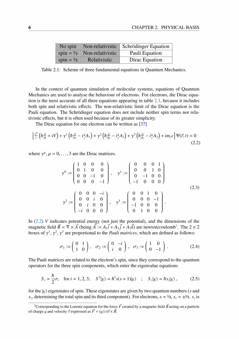
In the context of quantum simulation of molecular systems, equations of QuantumMechanics are used to analyse the behaviour of electrons. For electrons, the Dirac equa-tion is the most accurate of all three equations appearing in table 2.1, because it includesboth spin and relativistic effects. The non-relativistic limit of the Dirac equation is thePauli equation. The Schrödinger equation does not include neither spin terms nor rela-tivistic effects, but it is often used because of its greater simplicity.
The Dirac equation for one electron can be written as [37][γ0
c
(~ ∂∂t + iV
)+ γ1
(~ ∂∂x − i e
c A1
)+ γ2
(~ ∂∂y − i e
c A2
)+ γ3
(~ ∂∂z − i e
c A3
)+ imec
]Ψ(~r, t) = 0
(2.2)
where γµ, µ = 0, . . . , 3 are the Dirac matrices.
γ0 :=
1 0 0 00 1 0 00 0 −1 00 0 0 −1
, γ1 :=
0 0 0 10 0 1 00 −1 0 0−1 0 0 0
γ2 :=
0 0 0 −i0 0 i 00 i 0 0−i 0 0 0
, γ3 :=
0 0 1 00 0 0 −1−1 0 0 00 1 0 0
.(2.3)
In (2.2) V indicates potential energy (not just the potential), and the dimensions of themagnetic field ~B = ∇ × ~A (being ~A := A1~i + A2~j + A3~k) are newton/coulomb3. The 2 × 2boxes of γ1, γ2, γ3 are proportional to the Pauli matrices, which are defined as follows:
σ1 :=(
0 11 0
), σ2 :=
(0 −ii 0
), σ3 :=
(1 00 −1
). (2.4)
The Pauli matrices are related to the electron’s spin, since they correspond to the quantumoperators for the three spin components, which enter the eigenvalue equations
S i =~
2σi for i = 1, 2, 3; S 2|χ〉 = ~2s(s + 1)|χ〉 ; S z|χ〉 = ~sz|χ〉 , (2.5)
for the |χ〉 eigenstates of spin. These eigenstates are given by two quantum numbers (s andsz, determining the total spin and its third component). For electrons, s = ½, sz = ±½. sz is
3Corresponding to the Lorentz equation for the force ~F created by a magnetic field ~B acting on a particleof charge q and velocity ~v expressed as ~F = (q/c)~v × ~B.

2.1. QUANTUM MECHANICS 7
a discrete index for spinorial wavefunctions χ. We can define the spinorial wavefunctionsχ as follows
χsz := 〈sz|χ〉 (2.6)
where 〈sz| is the Hermitian adjoint of an eigenvector of S 3 with eigenvalue ~sz. Thepossible values of sz are −s,−s + 1,−s + 2, . . . ,+s − 1,+s. In agreement with equations(2.5) these values correspond to the spinorial eigenfunctions χ½(sz) and χ-½(sz), whichsatisfy
χ½(½) = 1 , χ½(-½) = 0 , (2.7a)χ-½(½) = 0 , χ−½(-½) = 1 . (2.7b)
The inclusion of both spin and relativistic effects in the Dirac equation (2.2) makesit specially accurate for systems of electrons. However, as it can be noticed in (2.2), thespin (implicit in the Dirac matrices) and the derivatives with respect to space and timeare coupled. This makes the solution of the Dirac equation be much more numericallycomplex than that of the Schrödinger equation (which matches the Dirac equation in thenon-relativistic limit and neglecting magnetic fields), and makes the latter to be preferredto the former whenever the lost of accuracy resulting from this choice is not decisive.The Dirac equation itself is used to simulate a few systems, as those containing heavynuclei [38–40], while the Schrödinger equation is preferred for lighter ones [41]. In bi-ological molecules simulations, the influence of spin-orbit terms is normally slow as aconsequence of the low atomic numbers of the atomic species involved. For example,most proteins are majorly formed by only five different species: Hydrogen (Z=1), Car-bon (Z=6), Nitrogen (Z=7), Oxygen (Z=8) and small amounts of Sulfur (Z=16). Nucleicacids also contain Phosphorus (Z=15), but typically not Sulfur. These six low-Z atomicspecies form an important subset or the simulated biomolecules family. This suggests thatthe Schrödinger equation with an appropriate potential can be useful for Biophysics [42].In condensed matter, the Schrödinger equation is appropriate for most systems [43], andthe Dirac equation is necessary for a few exceptions [44], like one dimensional systems,3D semiconductors with the diamond structure and no gap, and graphene [45].
The Pauli equation [46] is the Dirac equation in the non-relativistic limit. This equa-tion considers particles under the influence of an external magnetic field ~B = ∇ × ~A, whichcouples with the magnetic moments of the analysed particles. The Pauli equation [46] forone electron reads
i~∂
∂tΨ(~r, t) =
(1
2me
(−i~∇ −
ec~A)2
+ V(~r, t) + µB~σ~B)Ψ(~r, t) , (2.8)
where µB the Bohr magneton (a constant) and ~σ a vector whose three components are thethree 2 × 2 Pauli matrices. Wavefunctions which are solution of (2.8) have two compo-nents, each corresponding to one eigenvalue of the spin (½ and -½), so we can expressthem as a 2 × 1 vector
Ψ =
(ψ1( ~r, t)ψ2( ~r, t)
)(2.9)
or as the additionΨ = ψ1( ~r, t) χ½(sz) + ψ2( ~r, t) χ−½(sz) . (2.10)
8 CHAPTER 2. PHYSICAL BASIS
The size of magnetic terms in (2.8) is usually small (of the order of the difference ofenergy levels of electrons divided by 10,000) for low atomic numbers. For example, it isresponsible of the fine structure corrections in Hydrogen [47]. However, increasing theatomic number carries an increasing size of this term. This is the reason why, for electronsorbiting heavy nuclei, equations including spin, like Pauli’s or Dirac’s are usually required[38]. The Pauli equation is expected to be more accurate than the Schrödinger equation,but since it is definitely more complex, it is to be expected that in most cases it has a moretime-consuming solution (i.e., its computational cost is expected to be higher). Becauseof this, it is sometimes used to simulate systems with a small number of electrons [48, 49],like individual atoms.
If we neglect the magnetic terms (i.e., those including ~B and ~A) in the Pauli equationfor one electron (2.8), we obtain the Schrödinger equation for one electron
i~∂
∂tΨ(~r, t) =
(−~2∇2
2me+ V(~r, t)
)Ψ(~r, t) . (2.11)
For a system of N electrons, the Schrödinger equation is [47]
i~∂
∂tΨ(~r1,~r2, . . . ,~rN , t) = HΨ(~r1,~r2, . . . ,~rN , t) (2.12)
=
[−~2
2me
(∇2~r1
+ ∇2~r2
+ . . . + ∇2~rN
)+ V(~r1,~r2, . . . ,~rN , t)
]Ψ(~r1,~r2, . . . ,~rN , t) ,
where ~rα for α = 1, . . . ,N are the R3 vectors for positions of all N electrons. ~ is thePlanck constant divided by 2π and me is the electron mass at rest, while i :=
√−1. The
positions ~rα satisfy
∇2~rα
:=∂2
∂x2α
+∂2
∂y2α
+∂2
∂z2α
, for α = 1, . . . ,N . (2.13)
Equation (2.12) is also valid for N particles of mass m by replacing me in it by m. It isalso valid for N particles with different masses mα, α = 1, . . . ,N just by replacing theterms ∇~rα/me by ∇~rα/mα. The first term in the square brackets in the right hand side ofequation (2.12) corresponds to the kinetic energy of electrons, while the second one Vcorresponds to its potential energy. Operator H stands for the Hamiltonian. This Hamilto-nian does not include any term depending on electronic intrinsic angular momenta (spin),but spin-dependent terms can be included in its solutions. Antisymmetric functions arechosen for these solutions, what ensures the Pauli exclusion principle is satisfied. If thepotential energy does not depend on time explicitl, i.e., if ∂V
∂t = 0, then the total wave-function Ψ can be factorized into a time-dependent term times a coordinates-dependentterm (ψ(~r1,~r2, . . . ,~rN)), what gives rise to the time-independent Schrödinger equation forN electrons:
Eψ(~r1,~r2, . . . ,~rN) = Hψ(~r1,~r2, . . . ,~rN) (2.14)
=
[−~2
2me
(∇2~r1
+ ∇2~r2
+ . . . + ∇2~rN
)+ V(~r1,~r2, . . . ,~rN)
]ψ(~r1,~r2, . . . ,~rN) .
This is an eigenvalue equation, where E the eigenvalue associated to the eigenfunctionψ(~r1,~r2, . . . ,~rN). The physical meaning of E is that it is the energy of the system of Nelectrons.
2.1. QUANTUM MECHANICS 9
By multiplying (2.14) by the position operator eigenvectors |r〉 and integrating withrespect to~r, we obtain another form for the time-independent Schrödinger equation, whichinvolves quantum states and not wavefunctions:
E|Ψ〉 = H|Ψ〉 , (2.15)
where H is the Hamiltonian (with time-independent potential energy) which appears inthe Schrödinger equation. Equation (2.14) is the starting point of ab initio simulationmethods, like Hartree-Fock or Density Functional Theory methods, among others.
When dealing with molecules, the only interaction considered to take part in the po-tential energy V of the equations is frequently the electrostatic one. The velocities4 ofthe particles involved are assumed to be low enough to neglect electromagnetic effects, atleast for not very heavy atoms, as those involved in biological molecules, in physiologicalconditions. So, it is expected that keeping only electrostatics will suffice for many inter-esting phenomena. Regarding the importance of the electrostatic interaction, we dedicatea whole chapter —ch. 4— to study it.
When a system consisting of both nuclei and electrons is to be analysed using Quan-tum Mechanics, a completely rigurous treatment would demand wavefunctions dependingon both nuclear and electronic coordinates Ψ(X, x), where X are the spatial (R) and spino-rial components of all nuclei, and x are that of electrons. In order to save computationaltime, however, the use of the Born-Oppenheimer (BO) approximation is very popular inQuantum Chemistry. It consists of considering that nuclei move in the average electricfield created by electrons, and therefore sequentially solving the electronic system and thenuclear system. This approximation is justified by the relative slowness of nuclei motionwith respect to electronic motion. This slowness is attributable to the high quotient of thenuclear mass divided by electron mass for all atoms. For example, the lightest atom is theHydrogen one (the isotope without any neutron in its nucleus), for which this quotient isabout 1,800. In a common first row nuclei such as Carbon’s, this ratio is above 20,000.
In the BO framework, a time-independent Schrödinger equation is solved for the elec-trons (2.16a), assuming clamped nuclei. I.e., the nuclear positions are assumed to befixed, what makes the nuclear degrees of freedom to appear as parameters in the electronicSchrödinger equation (2.16a). When the electronic ground state wavefunction Ψ0
e(x; R) iscalculated, its energy (E0
e (R), depending on nuclear positions) is included in the Hamil-tonian for nuclei, and then the nuclear Schrödinger equation (2.16b) is solved. The set ofequations for the Born-Oppenheimer approximations is [50]
He(R)Ψ0e(x; R) :=
(Te + VeN(R) + W
)Ψ0
e(x; R) = E0e (R)Ψ0
e(x; R) , (2.16a)
HNΨN(X) :=(TN + WN(R) + E0
e (R))ΨN(X) = ENΨN(X) , (2.16b)
Ψ(x,X) ' Ψ0e(x; R)ΨN(X), E ' EN . (2.16c)
In equations (2.16), the term W indicates the pairwise electron-electron potential energy,the term WN indicates the nucleus-nucleus potential energy and the term VeN indicates theelectrons-nucleus potential energy. The semicolon in Ψ0
e(x; R) indicates that the nuclearpositions R are parameters when Ψ0
e is calculated. Equation (2.16c) represents a special
4When referring to quantum particles, of course, the concept of trajectory is meaningless, and the word’velocity’ may be replaced by an expression like 〈Ψ|P|Ψ〉/me, where P is the linear momentum operator.

10 CHAPTER 2. PHYSICAL BASIS
type of factorization of the total wavefunction of the system. More restricted factorizationsof the type Ψ(x,X) ' Ψ0
e(x)ΨN(X) are precluded by the potential energy term whichcouples electrons with nuclei VeN . In molecular simulations, it is common that the nucleiare considered classical particles. Therefore they are localized, and equations (2.16b) and(2.16c) are not used. In these cases, E0
e (R) acts as a potential energy term for the classicalnuclei.
There exist several (QM) methods to solve the Schrödinger equation of a system ofmany electrons (2.12). One of the simplest examples is the Hartree-Fock (HF) method[50]. It is based on a variational treatment of the Schrödinger equation, what impliesthat calculated HF energy is always higher than the actual ground state physical energy.Inaccuracies of the HF method [13] make it not appropriate for many purposes. It is stilluseful for qualitative estimations, as well as for calculations of the exchange potentials(see hybrid functionals in sec. 2.2).
Improvements in accuracy with respect to HF can be attained with the ConfigurationInteraction (CI) variational method, which uses a linear combination of Slater determi-nants as solution, instead of a single one or the Multi Configuration Self Consistent Field(MCSCF), which is similar in spirit, but technically different. Another approach to solve(2.12) is to use perturbative methods, like the Møller-Plesset (MP) family (with containsMP2, MP3, MP4, etc., depending on the perturbation order). Another hierarchy of meth-ods to solve the Schrödinger equation is the Coupled Cluster (CC) family, which is alsovery popular.
An alternative to tackle the Schrödinger equation (2.12), in a rather different mathe-matical formalism, is Density Functional Theory (DFT). In the framework of DFT onedoes not tackle the Schrödinger equation directly, but instead, one uses the Kohn-Shamequation. DFT has proven to be accurate and efficient at the same time for a large setof applications, and in this Ph. D. dissertation we are going to focus on it in the contextof metods based on Quantum Mechanics. In the following sections (2.2 and 2.3) we aregoing to review some fundamentals of Density Functional Theory and Time-dependentDensity Functional Theory (TDDFT), which are a central tool for quantum ab initio simu-lations. For more information about quantum ab initio methods for molecular simulation,see [51].
2.2 Density Functional TheoryIn section 2.1, the basic equations of Quantum Mechanics were presented. For simulationof molecules of biological systems at physiological conditions, the Schrödinger equationis commonly an appropriate choice. However, the choice of the method to solve theSchrödinger equation, or other equations derived by taking it as the starting point (forexample, the Kohn-Sham equations) is less clear. To this end there exist several methods,each having characteristic efficiency and accuracy. Many of them can be classified intowavefunction methods and density functional theory methods. Let us discuss now someof the fundamental aspects of the latter family of methods5.
We define xα := (~rα, (sz)α) = ((rx)α, (ry)α, (rz)α, (sz)α), being (rx)α, (ry)α, (rz)α the po-sitions in real space of the electron labeled with the index α, and being (sz)α the third
5The calculations presented in this section from this point on are largely based on refs. [52–54].
2.2. DENSITY FUNCTIONAL THEORY 11
component of its spin (see equations (2.5)). As solutions of the equations of a systeminvolving N electrons whose potential does not depend explicitly on time, wavefunctionmethods use functions Ψ(x1, x2, . . . , xN) depending on a set of N different xα vectors, be-ing α = 1, . . . ,N. Ψ(x1, x2, . . . , xN) is the wavefunction corresponding to a vector |Ψ〉 ofa Hilbert space, being |Ψ〉 the vector containing all the information about the quantumsystem that can be known. Since electrons are fermions, the wavefunction of a system ofN electrons should be antisymmetric. This is, by exchanging the positions of two indicesin the wavefunction, the resulting function must be minus the original one:
Ψ(. . . , xk−1, xk, xk+1, . . . , xl−1, xl, xl+1, . . .) = −Ψ(. . . , xk−1, xl, xk+1, . . . , xl−1, xk, xl+1, . . .) .(2.17)
The well-known Pauli exclusion principle is a consequence of antisymmetry. One simpleway to construct a wavefunction which is antisymmetric is the one used in the popularHartree-Fock method [50]. In HF, a Slater determinant, involving N one-electron func-tions φα with α = 1, . . . ,N is used.
A different approach is given by Density Functional Theory. In it, the basic mathe-matical function to solve a quantum equation of a system formed by N identical particlesis not the wavefunction (which depends on N variables xα), but the density function ρ(~r)(or more complicated functions) 6. By virtue of its efficiency, Density Functional Theory(DFT) methods have become very popular for simulation of many small-scale systems,including biological molecules. Although DFT can include both explicit spin and rela-tivistic corrections in the Hamiltonian of the tackled system, (see the Kohn-Sham-Diracequation in [52]), these are beyond the scope of this dissertation.
Given the wavefunction of a system of N electrons (Ψ), which is solution of the Schrö-dinger equation (2.14), we define
γN(x ′1 , . . . , x′
N; x1, . . . , xN) := Ψ∗(x ′1 , . . . , x′
N)Ψ(x1, . . . , xN) , (2.18a)γp(x ′1 , . . . , x
′p ; x1, . . . , xp) :=
:=(Np
) ∫dxp+1dxp+2 . . . dxN Ψ∗(x ′1 , . . . , x
′p , xp+1, . . . , xN)Ψ(x1, . . . , xp, xp+1, . . . , xN)
=
(Np
) ∫dxp+1 . . . dxN γN(x ′1 , . . . , x
′p , xp+1, . . . , xN; x1, . . . , xp, xp+1, . . . , xN)
for 1 ≤ p < N , (2.18b)ρp(x1, . . . , xp) := γp(x1, . . . , xp; x1, . . . , xp) =
=
(Np
) ∫dxp+1 . . . dxN Ψ∗(x1, . . . , xN)Ψ(x1, . . . , xN) for 1 ≤ p ≤ N , (2.18c)
where integrals sweep all possible values of spatial coordinates and spin components (in
6In this section we present the basic equations and methods of Density Functional Theory (relying on theKohn-Sham (KS) ansatz, KS-DFT). Other branches of increasing complexity of DFT, however, do exist. Forexample, if the Hamiltonians depend on spin and magnetic terms, the field studying the related problems isSpin Density Functional Theory; if both spin terms and relativistic corrections are included, the formalismis called Current Density Functional Theory [52]; if different densities are considered for different species,like electrons and nuclei, the field is Multicomponent Density Functional Theory [55]; etc.

12 CHAPTER 2. PHYSICAL BASIS
the latter case, integrals are actually summations). Equations (2.18) imply that
γ1(x ′1 ; x1) := N∫
dx2 . . . dxN Ψ∗(x ′1 , x2, . . . , xN)Ψ(x1, x2, . . . , xN) , (2.19a)
ρ2(x1, x2) :=N(N − 1)
2
∫dx3 . . . dxN Ψ∗(x1, x2, . . . , xN)Ψ(x1, x2, . . . , xN) , (2.19b)
ρ1(x1) := ρ(x1) := N∫
dx2 . . . dxN Ψ∗(x1, x2, . . . , xN)Ψ(x1, x2, . . . , xN) , (2.19c)
ρ(~r1) :=∑
s1
ρ(x1) = N∑
s1
∫dx2dx3 . . . dxN Ψ∗(x1, x2, . . . , xN)Ψ(x1, x2, . . . , xN) .
(2.19d)
In equation (2.19d) a summation for the possible values of spin of one particle of thesystem is evaluated. This equation is to be highlighted, because it defines the electronicdensity, whose use is the basis of Density Functional Theory7. The first three quantitiesof (2.19) suffice to calculate the ground state energy E (2.14) of a quantum system. Theexpresion for the ground state energy can be calculated just by using the antisymmetryproperty of Ψ (2.17) and the mathematical property that any function f (~rα) depending on~rα satisfies
f (~rα) =
∫d~r f (~r) δ
(~r − ~rα
), (2.20)
where δ is the Dirac delta and the integral is performed in the whole space. Therefore,if we transform the time-independent Schrödinger equation (2.15) by using (2.17) and(2.20), and we express the result according to definitions (2.19), we reach
E|Ψ〉 = H|Ψ〉H = T + V + W
=⇒ E = 〈Ψ|H|Ψ〉 = 〈Ψ|T + V + W |Ψ〉 =
−
∫dx ′1
(~2
2me∇2~r1γ1(x ′1 ; x1)
)∣∣∣∣∣∣x1=x ′1
−
∫dx1
M∑µ=1
e2Zµ
4πε|~r1 − ~Rµ|
ρ(x1)
+
∫dx1dx2
e2ρ2(x1, x2)4πε|~r1 − ~r2|
, (2.21)
where |Ψ〉 is the ground state of the system, me and e are the mass and the electric chargeof the electron, ε is the dielectric constant of the medium (usually the vacuum), and M isthe number of the pointlike sources of electric charge like atomic nuclei, whose positionsare ~Rµ
8. The terms of the Hamiltonian are defined as
T := −N∑α=1
~2
2me∇2~rα, (2.22a)
V := −N∑α=1
M∑µ=1
e2Zµ
4πε|~rα − ~Rµ|, (2.22b)
W :=N∑α=1
N∑β>α
e2
4πε |~rα − ~rβ|, (2.22c)
7At least for its basic version of DFT, not including spins.8In eq. (2.21) it is assumed that the wavefunction is normalized. Otherwise, E = 〈Ψ|H|Ψ〉/〈Ψ|Ψ〉.

2.2. DENSITY FUNCTIONAL THEORY 13
where ~r1 and ~r2 stand for electron positions. The first term on the right hand side of eq.(2.21) corresponds to the quantum kinetic energy of electrons, while the third one repre-sents the potential energy associated to the interaction among the electrons themselves.The second term on the right hand side of eq. (2.21), coming from (2.22b), correspondsto the external potential created by the nuclei and acting on the system of N electrons. Init, the term in brackets is the external potential operator V(x1), and therefore this secondterm equals
〈Ψ| V |Ψ〉 =
∫dx1 V(~r1)ρ(x1) = −
∫dr1
M∑µ=1
e2Zµ
4πε|~r1 − ~Rµ|ρ(r1) . (2.23)
Definitions (2.18b), (2.18c) imply that
ρ2(x1, x2) = γ2(x1, x2; x1, x2) , (2.24a)
γ1(x′1; x1) =2
N − 1
∫dx2 γ2(x′1, x2; x1, x2) . (2.24b)
Therefore, γ2(x′1, x2; x1, x2) would suffice to calculate the energy in (2.21), without ex-plicit need of the wavefunction Ψ. One may think that a new formalism based on γ2 maybe used as an alternative to the wavefunction formalism of Quantum Mechanics. Thisformalism is called second order matrix density theory. Although using this formalismis possible, at present it is too computationally demanding, and that is the reason why itis not widely used. Instead, a theory where the basic magnitude is ρ(~r) (or ρ(~r)), Den-sity Functional Theory, is used to overcome the complexity arising from the excess ofelectronic coordinates characteristic to the wavefunction formalism.
Density Functional Theory is based on the Hohenberg-Kohn Theorem [56], (alsoknown as the first Hohenberg-Kohn Theorem) which states:
For ρ0(~r) corresponding to the non-degenerate ground state produced by any externalpotential (i.e., for V-representable densities), this potential V is univocally determinedby ρ0(~r), except for an additive constant. Since V determines the Hamiltonian H of thesystem, ρ0(~r) also determines the wavefunctions corresponding to the ground state and toall excited states. This is,
Ψk(x1, x2, . . . , xN) = Ψk([ρ0]; x1, x2, . . . , xN) , (2.25)
where k labels the entire spectrum of the many-body Hamiltonian H.
Consider a system of N electrons described by a quantum Hamiltonian (like the onedisplayed in equation (2.14)) whose terms do not depend on time explicitly. The Hohenberg-Kohn Theorem implies that its non-degenerate ground state |Ψ〉 (if it exists) correspondsto a given ground state electronic density ρ0(~r) (2.19d), and that there exist one and onlyone potential function V(~r) for a given ρ0(~r). In this context, we consider potentials beingdifferent in just one additive constant as equivalent potentials (V1 ≡ V2 if V1 = V2 + k,being k a constant). The Hohenberg-Kohn Theorem can be proved by reductio ad absur-dum as follows. Consider that there do exist two different potentials V1(~r), V2(~r) beingdifferent in more than one constant, and both correspond to the same given ground state

14 CHAPTER 2. PHYSICAL BASIS
density ρ0(~r). We will first prove that two potentials V1(~r), V2(~r) being different in morethan one constant cannot have a common ground state (also by reductio ad absurdum).Assume V1(~r) and V2(~r) have a common ground state |Ψ〉. Then,
H1|Ψ〉 = (T + W + V1)|Ψ〉 = E1|Ψ〉 , H2|Ψ〉 = (T + W + V2)|Ψ〉 = E2|Ψ〉 . (2.26a)
If we subtract both equations, we reach
(V1 − V2)|Ψ〉 = (E1 − E2)|Ψ〉 . (2.27)
Since (E1 − E2) is a constant, and |Ψ〉 cannot be zero except in a small set of points, wehave reached a contradiction: V1 and V2 are different only in one constant. Therefore,we conclude that two potentials being different in more than one constant cannot havea common ground state, but two different ground state vectors |Ψ1〉 and |Ψ2〉. The non-degeneracy of the ground state makes
〈Ψ1|H1|Ψ1〉 < 〈Ψ2|H1|Ψ2〉 , (2.28)
because the energy of any state |Ψ′〉 should be strictly higher than that of the ground state.If we call E1 and E2 to the energies of the ground states |Ψ1〉 and |Ψ2〉, then (2.28) implies
E1 < 〈Ψ2|H1|Ψ2〉 = 〈Ψ2|H2|Ψ2〉+〈Ψ2|(V1(~r)−V2(~r))|Ψ2〉 = E2+
∫d~r ρ0(~r)
(V1(~r) − V2(~r)
).
(2.29)In order to derive (2.29), we have used the fact that in the Hamiltonians H1 and H2, corre-sponding to two systems of N electrons, the kinetic term and the potential energy term dueto electron-electron interactions are identical. The external potential is the only differentterm, and thus H1 = H2 − V2 + V1. We have also used that 〈Ψ|V(~r)|Ψ〉 =
∫d~r ρ0(~r)V(~r)
(see eq. (2.21)). Operating in an analogous manner, we obtain
E2 < 〈Ψ1|H2|Ψ1〉 = E1 +
∫d~r ρ0(~r)
(V2(~r) − V1(~r)
). (2.30)
Gathering together equations (2.29) and (2.30) we reach a contradiction:
E1 + E2 < E1 + E2 , (2.31)
what proves the first Hohenberg-Kohn Theorem. If we call (ρ0)i, i = 1, 2 to the electronicdensities corresponding to the ground state of systems of N electrons whose externalpotentials are V1, V2, this proves that
((ρ0)1 = (ρ0)2)⇒ (V1 = V2) . (2.32)
The converse ((ρ0)1 = (ρ0)2) ⇐ (V1 = V2) is obvious. Accordingly, there is a bijectionbetween densities and potentials up to a constant: ((ρ0)1 = (ρ0)2)⇔ (V1 = V2). Since adensity ρ0(~r) corresponding to the ground state determines a potential V(~r), it also de-termines the explicit form of the Hamiltonian and that of the Schrödinger equation, andtherefore it determines all its solutions (ground state and excited states).
The formulation of the Schrödinger equation (ignoring the Hohenberg-Kohn Theo-rem) ensures that, for a system of N electrons and M atomic nuclei, the knowledge
2.2. DENSITY FUNCTIONAL THEORY 15
of nuclear positions (~Rµ for µ = 1, . . . ,M) and corresponding atomic numbers (Zµ forµ = 1, . . . ,M) makes the Hamiltonian H known. The knowledge of this Hamiltonianmakes it possible to calculate both the ground state energy E0 and the correspondingground state wavefunction Ψ0(x1, . . . , xN); this wavefunction determines the ground stateelectronic density ρ0(x):
N,Zµ,Rµ for µ = 1, . . . ,M ⇒ H ⇒
Ψ0 ⇒ ρ0(~r)E0
. (2.33)
The Hohenberg-Kohn Theorem enables the mapping in the opposite direction. The knowl-edge of the ground state density ρ0(~r) makes the potential known, what makes nuclei’s po-sitions and atomic numbers also known. As we said before, this makes the HamiltonianH known, what (at least formally) enables to calculate the wavefunction and the energyof the ground state:
ρ0(~r) ⇒ N,Zµ,Rµ for µ = 1, . . . ,M ⇒ H ⇒
Ψ0
E0. (2.34)
Equatioms (2.33) and (2.34) form a closed loop: the knowledge of the Hamiltonian Henables the calculation of the density ρ and the converse. The bijection between groundstate density and ground state energy ρ0(~r) ⇔ E0 makes it possible to define the followingthree functionals of the ground state density
T [ρ0] :=〈Ψ|T |Ψ〉 , (2.35a)
ENe[ρ0] :=〈Ψ|V |Ψ〉 , (2.35b)
Eee[ρ0] :=〈Ψ|W |Ψ〉 . (2.35c)
All three functionals are univocally determined by the ground state density ρ0(~r). Thelinearity of the operators T , V and W (see (2.22)), together with (2.21), yields
〈Ψ0|H|Ψ0 〉 = E[ρ0] = T [ρ0] + ENe[ρ0] + Eee[ρ0] . (2.36)
The relations T = T [ρ0] and Eee = Eee[ρ0] of equations (2.35) are only valid for non-degenerate ground states, because in these cases there exist a bijection |Ψ0〉 ⇔ ρ0. If theground state is degenerate, these relations are no longer satisfied, but anyway, there exista functional F = F[ρ0] which explicitly depends on the ground state density [57], andwhich is defined as
FHK[ρ(~r)] := E[V[ρ(~r)]] −∫
d~r V[ρ(~r)]ρ(~r) = T + Eee , (2.37)
i.e., as the energy of the quantum system (which is determined by the electronic densityρ, by virtue of the Hohenberg-Kohn Theorem) minus the potential energy (which is alsodetermined by ρ, by virtue of (2.23)). The value of this functional matches that of theinternal energy (T + Eee). This functional is called the Hohenberg-Kohn functional FHK
for a given system of electrons under a known external potential V .It is to be stressed that only the ground state density ρ0 can lead to the information
of positions and atomic numbers of nuclei which is necessary to establish the mappingbetween the density and the potential. The density of an excited state cannot be used for

16 CHAPTER 2. PHYSICAL BASIS
this purpose, because in this case the demostration of the Hohenberg-Kohn Theorem (seeearlier in this section) would not be valid.
The bijection between external potentials V and densities ρ (enabled by bijections tothe wavefunction Ψ)
V(~r)1⇐⇒ Ψ(~r1,~r2, . . . ,~rN)
2⇐⇒ ρ(~r) (2.38)
can be broken out of two different phenomena: degeneracy and non-uniqueness [57].Mapping 1 can break down (i.e., cease to be biunivocal) if two different potentials maponto the same wavefunction Ψ. This fact is called non-uniqueness, and can happen alreadyin charge-density-only DFT if finite basis sets are taken to represent Ψ (what is alwaysthe case for real-world simulations). In multi-density DFT’s, like Spin Density FunctionalTheory and Current Density Functional Theory, which involve other basic variables apartfrom ρ(~r), mapping 1 can also break down even in the complete basis set limit, because theinversion of the Schrödinger equation does not establish a unique relation between the setof densities and the set of conjugate potentials [58]. Mapping 2 can break down if differentwavefunctions Ψ correspond to the same ground state density ρ, what is called degeneracy(because it happens for degenerate ground states). The proof of the Hohenberg-KohnTheorem presented above was based in the non-degeneracy of the ground state. Hence,the Hohenberg-Kohn Theorem is no longer valid for degenerate ground states, what isquite common in molecular simulation [52]. However, the validity of Density FunctionalTheory can be restored for these cases, for it can be proven that regardless of any possibledegeneracy or non-uniqueness, two different systems with the same ground state densityhave the same internal energy
〈Ψ|T + W |Ψ〉 = FHK[ρ(~r)] , (2.39)
[57], and therefore the density and the external potential suffice to calculate the energy ofthe quantum system (i.e., no explicit wavefunction is required).
We define the setAρ
Aρ := ρ(~r) | ρ comes from an N-particle ground state |Ψ〉 . (2.40)
Since the energy of the ground state of a quantum system is minimal, the following prop-erty holds
E[V] = minρ ∈ Aρ
FHK[ρ] +
∫d~r V[ρ]ρ
. (2.41)
This relation is called the variational Hohenberg-Kohn Theorem (or the second Hohenberg-Kohn Theorem), and it has strong implications in the procedure to calculate ρ(~r), as wewill see later in this section.
The (first) Hohenberg-Kohn Theorem stated earlier in this section is an existence the-orem, but not a constructive one. This is, it does not give itself information on howthe electronic density can be calculated if the potential V is known, what is usually thecase in molecular simulation (to calculate the quantum state of electrons if the nucleipositions are known; it is useful because the electronic state strongly influences the mo-tion of the nuclei). DFT-based calculations are feasible thanks to the simplified solutionscheme of Kohn-Sham [59], which transforms a computationally heavy many electron

2.2. DENSITY FUNCTIONAL THEORY 17
problem into a computationally more tractable problem of noninteracting electrons [60].So far we have considered Hamiltonians H = T + V + W for a given N-electron system.These Hamiltonians are called interacting Hamiltonians because they contain the term W(2.22c) of electron-electron interaction. The so-called Kohn-Sham ansatz consists of sup-posing that, for any N-electron system, there exist a so-called noninteracting HamiltonianHs := T + Vs = − ~
2
2me
∑α ∇~rα +
∑α Vs(~rα) which lacks the electron-electron term (W := 0)
and whose external potential energy (Vs) is such that the density ρ corresponding to boththe interacting and noninteracting Hamiltonians is the same. Vs is obtained through a pro-cedure that we will explain further in this section. The lack of an electron-electron termstrongly simplifies the calculations. Since electrons are not interacting among themselves,the the ground state Φ of the noninteracting system of N electrons (whose Hamiltonian isHs) can be a Slater determinant:
Φ(x1, x2, . . . , xN) =1√
N!
∣∣∣∣∣∣∣∣∣∣∣∣φ1(x1) φ2(x1) . . . φN(x1)φ1(x2) φ2(x2) . . . φN(x2)...
.... . .
...φ1(xN) φ2(xN) . . . φN(xN)
∣∣∣∣∣∣∣∣∣∣∣∣ , (2.42)
where the spin orbitals φα(xβ) (also called natural spin orbitals or Kohn-Sham orbitals)are subject to the orthonormality constraint
〈φα|φβ〉 = δα,β . (2.43)
We will call Ψ the solution wavefunction of the total interacting system, whose Hamilto-nian does include an electron-electron interaction term W, and Φ the wavefunction of thenoninteracting Kohn-Sham system. By virtue of (2.19c), and applying the antisymmetryproperty (2.17), eq. (2.42) leads to
ρ0(~r) =
N∑α=1
1/2∑sz=−1/2
φα(x)∗φα(x) =
N∑α=1
1/2∑sz=−1/2
|φα(~r, sz)|2 , (2.44)
if the Kohn-Sham ansatz is assumed to hold. This expression for the density correspondsto the particular case where the wavefunction is one Slater determinant (and not a linearcombination of infinite Slater determinants). In this case, we only have N different spinorbitals, whose occupation number is 1.
We derive the basic expression of the Kohn-Sham equations, which are used to cal-culate the electronic density ρ of a N-electron system with Hamiltonian H = T + V +
W (the Hamiltonian of the Schrödinger equation). By hypothesis, ρ is interacting V-representable, i.e., ρ is the density which gives the correct energy E of a N-electron sys-tems whose Hamiltonian is H = T + V + W. This interacting Hamiltionian is determinedby the external potential V , and contains an electron-electron interaction term W. Thebasic assumption of Kohn-Sham is that this ρ is also noninteracting V-representable. I.e.,that the same ρ also gives the same correct energy E for a Hamiltonian Hs = T + Vs lack-ing W term, and whose external potential term Vs is specially arranged to this end. In bothcases (interacting and noninteracting Hamiltonian), the wavefunction corresponding to ρ,according to (2.19c), is the solution of the time-independent Schrödinger equation with

18 CHAPTER 2. PHYSICAL BASIS
the corresponding Hamiltonian (H for the interacting system, Hs for the noninteractingsystem). In the hypothesis of Kohn and Sham, the energy of the system is
E = 〈Φ|Hs|Φ〉 =
N∑α=1
(∫dx φ∗α(x)Tφα(x) +
∫d~r ρ(~r)Vs
)
=
N∑α=1
∫dx
−φ∗α(x)~2∇2
~r
2meφα(x) + φ∗α(x)Vs(~r)φα(x)
. (2.45)
The variational Hohenberg-Kohn Theorem (2.41) states that the energy of the sys-tem should be minimal. Since the Kohn-Sham ansatz requires orthonormal spin orbitals(2.43), these conditions should be included as constraints in the minimization equation9.Therefore, we define the functional
Ω[ρ] := E[ρ[φα]] −N∑α=1
N∑β=1
λα,β(〈φα|φβ〉 − δα,β) , (2.47)
whose minimum stationary condition
δΩ[ρ[φα]] = 0 , (2.48)
is ensured by the variational Hohenberg-Kohn Theorem. If we perform the functionalderivative10 of Ω[ρ[φα]] (with respect to φ∗α(x)), we obtain
hsφα(x) =
(−~2∇2
2me+ Vs(x)
)φα(x) =
N∑β=1
λα,βφβ(x) , (2.49)
where the effective Hamiltonian is defined as hs :=(−~
2∇2
2me+ Vs(x)
). The matrix λα,β in
(2.49) is a Hermitian matrix. The effective Hamiltonian hs is a Hermitian operator, andhence λα,β is a Hermitian matrix, which can be diagonalized by a unitary transformationof the orbitals. This transformation leaves invariant the (Slater) determinant (2.42), andhence leaves invariant the density (2.44) as well. Therefore, the Hamiltonian hs in (2.49) isalso unchanged by this transformation [54]. Consequently, the appropriate unitary trans-formation on spin orbitals φα makes equation (2.49) become
hsφα(x) =
(−~2∇2
2me+ Vs(x)
)φα(x) = λαφα(x) , α = 1, . . . ,N . (2.50)
The functional derivative of Ω[ρ[φα]] with respect to φ and φ∗ results into N equations.Equation (2.50) is an eigenvalue equation, where λα are the eigenvalues.
9If we want to minimize any functional F[φ] (depending on a function φ) which is subject to N con-straints σγ[φ] = 0, γ = 1, . . . ,N we must minimize the new functional
F[φ] −∑γ
λγ σγ[φ] , (2.46)
where the scalars λγ indicate the Lagrange multipliers, which are unknowns to be calculated.10For a definition of the functional derivative, see the appendices of [50].

2.2. DENSITY FUNCTIONAL THEORY 19
We perform an analogous procedure with the interacting system Hamiltonian H =
T + V + W. We will first re-express the energy of the system as
E[ρ] = Ts[ρ] + J[ρ] + Exc[ρ] + V[ρ] , (2.51)
being
Ts[ρ] := 〈Φ|T |Φ〉 = −~2
2me
N∑α=1
〈φα|∇2|φα〉 , (2.52a)
J[ρ] :=e2
2
∫d~r1d~r2
ρ(~r1)ρ(~r2)4πε |~r1 − ~r2|
, (2.52b)
V[ρ] :=∫
dx ρ(~r)V =
∫d~r ρ(~r)
M∑µ=1
−e2Zµ
4πε|~r − ~Rµ|
, (2.52c)
Exc[ρ] := T [ρ] − Ts[ρ] + W[ρ] − J[ρ] . (2.52d)
It is to be stressed that Ts in (2.52a) satisfies
Ts[ρ] = minΦ→ρ〈Φ|T |Φ〉 , (2.53)
i.e., the Slater determinant wavefunction Φ is the one, among all those corresponding tothe same given ρ (see (2.44)), which minimizes the kinetic energy.
Definitions (2.52) ensure that the energy (2.51) equals the total energy of the wholeinteracting system for a given density ρ. Because of the Hohenberg-Kohn theorem, all en-ergy terms must be determined by this electronic density. However, the energy in (2.51)is expressed as a function of the functions φα which determine the solution of the non-interacting system (2.42), taking (2.44) into account. This is because, as stated earlierin this section, the Kohn-Sham ansatz assumes the correct density ρ is the same for boththe interacting system and for the noninteracting system. The term J[ρ], called Hartreepotential, classical potential or electrostatic potential, corresponds to the classical part ofthe electron-electron potential of the interacting system. Its formula matches the classicalelectrostatic formula for charge distributions. In chapter 4 we perform an extended studyon efficient ways to calculate this term, whose accuracy and computational cost are crit-ical for molecular simulations. The term Ts[ρ] := 〈Φ|T |Φ〉 (2.52a) represents the kineticenergy of the noninteracting system in (2.51). It is expected to contain most of the actualkinetic energy of the interacting system T [ρ] := 〈Ψ|T |Ψ〉 (2.22a), but a small correction,which is included in the exchange correlation energy Exc (2.52d). Exc also contains thenon-classical part of the electron-electron potential of the interacting system W (2.22c).The exchange correlation energy is typically only a small part of the total energy of a sys-tem, although it is also commonly responsible of an important part of the forces bindingatoms together [60]. Once again, the functional
Ω[ρ] := E[ρ[φα]] −N∑α=1
N∑β=1
λα,β(〈φα|φβ〉 − δα,β) , (2.54)
is minimum, satisfying the stationary condition
δΩ[ρ[φα]] = 0 , (2.55)

20 CHAPTER 2. PHYSICAL BASIS
by virtue of the variational Hohenberg-Kohn Theorem. In this case, the functional deriva-tive of E[ρ] is
δE = δTs +
∫d~r δρ(~r)
[V(~r) +
∫d~r ′
e2ρ(~r ′)4πε|~r − ~r ′|
+ Vxc(~r)], (2.56)
withVxc(~r) :=
δExc[ρ′]δρ′(x)
∣∣∣∣∣ρ′=ρ
. (2.57)
By using eq. (2.50) and the Green’s Theorem, we obtain [61]
δTs = −
∫d~r Vs(~r)δρ(~r) . (2.58)
By gathering together eqs. (2.54), (2.55), (2.56), (2.58), inserting then the resulting Vs
expression into (2.50) and diagonalizing the λα,β matrix (this leaves invariant the Hamil-tonian) and redefining the Lagrange multipliers, we obtain the celebrated Kohn-Shamequations [54] in their canonical form
hsφα(x) =
(−~2∇2
2me+ Vs(~r)
)φα(x) = λαφα(x) , (2.59a)
Vs(~r) = V(~r) + e2∫
d~r ′ρ(~r ′)
4πε|~r − ~r ′|+ Vxc(~r) , (2.59b)
ρ(~r) =
N∑α=1
1/2∑sz=−1/2
φα(x)∗φα(x) , (2.59c)
where we have also included (2.44).The exchange correlation potential Vxc(~r) is defined in (2.57) as the functional deriva-
tive of the exchange correlation energy Exc(~r) (2.52d) with respect to the density ρ(~r) forthe density which minimizes the energy E (i.e., for the correct physical electronic den-sity). The derivation of the expression of Vxc(~r) is far from trivial. Up to this point, if weassume that non-relativistic Quantum Mechanics is correct and the magnetic terms in theHamiltonian are negligible, all calculations are still exact11. However, in this point furtherapproximations must be performed, since nowadays it does not exist an expression forthe exact exchange correlation potential Vxc(~r). As stated in [54], ’the search for an ac-curate exchange correlation term has encountered tremendous difficulty and continues tobe the greatest challenge in the Density Functional Theory’. There exist several methodsto calculate approximations to Exc, among which we can mention the popular Local Den-sity Approximation [62], Generalized Gradient Approximation [63] and hybrid functionalmethods as B3LYP [64]. Yet, none of them can avoid to make an error when calculatingthe density ρ.
We briefly explain the fundamentals of the Local Density Approximation (LDA). LDAis a simple and efficient approach to calculate the exchange correlation potential, butpresents accuracy drawbacks, as the underestimation of ionization energies. The LocalDensity Approximation consists of assuming a local relation with ρ(~r) when calculating
11If the Hamiltonian depends on spin-magnetic terms, and its solution is treated in terms of the electronicdensity, then the method is called Spin Density Functional Theory (SDFT) [60].

2.2. DENSITY FUNCTIONAL THEORY 21
the exchange correlation potential Vxc(~r). I.e., the value of Vxc(~r) at a given point ~r isassumed to depend just on the value of the density in that very point ρ(~r), and not on thevalues of the density in other points ρ(~r ′) with ~r ′ , ~r. The LDA is used in a variety ofdifferent methods [65–69]. Such methods split the exchange correlation energy into twocontributions
Exc = Ex + Ec , (2.60)
being Ec the correlation contribution, and being Ex the exchange contribution, whichcan be qualitatively understood as due to the fermionic exclusion of electrons. Both aretaken from a reference system, which is the Homogeneous Electron Gas (HEG)12. TheHEG [70] is a model system, consisting of a set of infinite electrons (N → ∞) in aninfinite-volume space (V → ∞), such that the overall charge density N/V equals a givenfinite value ρ. A homogeneous positive background charge distribution is present in theHEG, so that the net total electric charge is null. The HEG is a model which is based onstrict assumptions, and therefore is not expected to be very realistic for the description ofelectrons in many systems. However, in certain limits, it is the only system having knownanalytical expressions for its exchange correlation potential [70], and these expressionscan be used into many systems whose Vxc are unknown, providing reasonable results.
By hypothesis, the exchange correlation energy of any system, according to the LocalDensity Approximation is [54]
ELDAxc [ρ] =
∫d~r ρ(~r)εxc(ρ(~r)) , (2.61)
where εxc(ρ(~r)) is the exchange correlation energy per particle of a Homogeneous Elec-tron Gas having electronic density ρ. By definition (2.57), the corresponding exchangecorrelation potential is
Vxc(~r) =δExc
δρ(~r)= εxc(ρ(~r)) + ρ(~r)
δεxc
δρ(~r). (2.62)
The variable εxc is (arbitrarily) split into two parts
εxc(ρ(~r)) = εx(ρ(~r)) + εc(ρ(~r)) . (2.63)
Commonly, the exchange term εx is by far greater than the correlation term εc [60]. Thisis true not only for the HEG, but for a variety of systems. The correlation energy of anoninteracting uniform electron gas can be calculated by using the HF method [54], andprovides an analytic expression for this correlation energy as a function of the electronicdensity:
εx(ρ(~r)) = −34
(3π
)1/3
ρ(~r)1/3 . (2.64)
The correlation term, in contrast, is more elusive. Its analytical expressions are onlyknown for the limits of high and low density of the HEG. They can be calculated through
12Sometimes also called Uniform Electron Gas

22 CHAPTER 2. PHYSICAL BASIS
perturbative series, giving approximate results per electron [71, 72]
εc = 0.0311ln(rs) − 0.048 + 0.009rsln(rs) − 0.018rs high density limit; (2.65a)
εc = −1.792
rs+
2.660
r3/2s
+br2
slow density limit; (2.65b)
rs :=(
34π
)1/3 mee2
4πε0e2ρ−1/3 . (2.65c)
In (2.65), me is the electron mass, e is the electron charge, ε0 the dielectric permittivityof the vacuum and b a parameter whose value is close to 0 [71]. As we can see, allthese terms depend on the density ρ in just one point, and do not require derivativesor integrals of ρ. If we use (2.65) into (2.62), we will notice that so does Vxc. Thereexist virtually infinite possible choices for εc. Many ones have given rise to popularconcrete LDA methods. Quantum Monte Carlo calculations are specially appropriate todetermine appropriate correlation energies. For example, interpolation of results obtainedvia Quantum Monte Carlo methods is used to build the correlation term of the popularLDA-VWN method [54, 69].
The calculation methods explained above are based on strict assumptions, and conse-quently one might think that the Local Density Approximation cannot produce accurateresults. However, its validity can be confirmed when checking that DFT-LDA calculationsgenerates results which are in good agreement with either experimental data or higher ac-curacy calculation methods. Drawbacks of LDA are the underestimation of charge tranferenergies, and a lack of accuracy of van der Waals interactions [73].
The Generalized Gradient Approximation (GGA) is another method to calculate Vxc.It goes one step further than LDA, because it uses exchange correlation terms dependingon both the electronic density ρ and on its gradient ∇ρ. Instead of (2.61), GGA uses
EGGAxc [ρ] =
∫d~r ρ(~r)εxc(ρ(~r),∇ρ(~r)) . (2.66)
If GGA and LDA (both including spin) are compared, GGA is found to produce bet-ter total energies, atomization energies, energy barriers and structural energy differences[74]. GGA methods can often predict geometries and vibrational frequencies for stablemolecules with the same or even more accuracy than MP2 methods, at a computationalcost of the order of Hartree-Fock methods [51]. For several purposes, gradient correctedmethods perform much better than LDA [51]. When calculating other quantities, how-ever, we could say that GGA gives a slightly better accuracy than LDA at a slightly highercomputational cost (see chapter 5).
Greater accuracy than GGA and LDA, commonly at a cost of higher numerical com-plexity, can be obtained by using hybrid functionals. Hybrid functionals do not merelyuse the exchange potential term corresponding to a HEG, but analytically calculate theexchange term of the analysed system using the Hartree-Fock method, to include it inVxc. The HF method handles Slater determinants, and thus can properly calculate the ex-change term. For example, a popular hybrid functional is B3LYP13 [64]. The exchange
13This name is an acronym for Becke - 3 parameter - Lee/Yang/Parr. It receives this name because of thecontributions of the mentioned researchers.

2.2. DENSITY FUNCTIONAL THEORY 23
correlation energy of B3LYP is
EB3LYPxc [ρ] = (2.67)
ELDAxc [ρ] + a0
(EHF
x [ρ] − ELDAx [ρ]
)+ ax
(EGGA
x [ρ] − ELDAx [ρ]
)+ ac
(EGGA
c [ρ] − ELDAc [ρ]
),
where EHFx indicates the exchange energy of the Hartree-Fock method. The three param-
eters are fit to reproduce heats of formation of small molecules, and their values in thestandard B3LYP are a0 = 0.20, ax = 0.72 and ac = 0.81. For the LDA part, the function-als presented in [69] are to be used. The term multiplying ax is the Becke correction tothe exchange functional presented in [75]. The term multiplying ac is the Perdew-Wangcorrection to the correlation functional presented in [76].
Once the expression for the exchange-correlation term is chosen, the next step is tosolve the Kohn-Sham equations (2.59), what is made in an iterative manner. In fig. 2.1 weschematically depict the main steps of this process. First, an initial guess of the density(i.e., an assumption of a given form of ρ0(~r)) is made. Then, a sequence of iterationsstarts. In iteration i, the effective Kohn-Sham potential V i
s[ρi] is calculated for a given
density ρi. This potential is inserted in the Kohn-Sham equations, which are then solved,what generates new φα spin orbitals , and therefore a new density ρi+1 by using (2.44). Thisnew density can be the input for a new iteration. This process is repeated until a tolerancein some variable is reached (for example, until the variation in the integral of the modulusof ρi − ρi−1 for all space is below a given chosen value). When this happens, we say thecalculations are self-consistent. The loop can also be stopped after a chosen number ofiterations even if the self-consistency criterion has not been satisfied, to avoid too longexecution times and infinite loops. When the iterations are finished, the quantities wewanted to calculate are computed, if they were not found during the self consistent fieldprocess.
The starting point of section 2.1 was the Dirac equation, which is expected to bevery accurate for the analysis of systems of electrons. From that starting point, and upto this point, we have made several assumptions (to neglect relativistic corrections andspin-dependent Hamiltonians, to calculate Vxc by using results from the HEG, etc.). Theaccumulation of assumptions may lead us to have some doubts about the capability ofDFT, for example in LDA and GGA approximations, to provide reasonable results whenused to analyse physical systems. A simple example can help us to dispel our doubts. Infigures 2.2 and 2.3, we display the electronic density of two systems, CH4 and the chro-mophore of the Green Fluorescent Protein [34, 35]. These densities were calculated bothwith DFT-LDA and DFT-GGA using the Octopus code [6], and plots were made usingXCrySDen [78]. The electronic density for a given isovalue14 is plotted as a blue cloud,atoms are represented by spheres and covalent bonds are represented by rods connectingthem. In both figures 2.2 and 2.3, we can easily notice that the electron density occupiespreferentially the regions corresponding to covalent bonds. This explains a physical phe-nomenon, because bonding results from the existence of negative charges lying midwaybetween the positively charged nuclei, what keeps together the nuclei. This is a simplequalitative example, though there is a vast number of examples in the literature which con-firm the reliability of DFT when calculating observable quantities. For example, in [79],enthalpies of formation at 298 K are calculated for a set of 148 different molecules and
14Constant value of the density ρ(~r).

24 CHAPTER 2. PHYSICAL BASIS
Figure 2.1: Scheme of the self-consistent field algorithm to perform calculations on a quantumsystem according to Density Functional Theory using Kohn-Sham equations [77].

2.2. DENSITY FUNCTIONAL THEORY 25
Figure 2.2: Example of how DFT explains the existence of bonds in a molecule (CH4). The elec-tronic density at a given isovalue is represented as a blue cloud. A) Using LDA-VWN functional[69]; B) Using GGA-PBE functional [63, 74].
then compared with experimental values. The mean square deviation for DFT predictionsis found to be 90.9 kcal/mol for (VWN) Spin-LDA, 7.1 kcal/mol for (BLYP) GGA and3.1 kcal/mol for B3LYP. In addition to quantitative results like these, the bonding examplejust presented can help to visualize the power of Quantum Mechanics ab initio methods ingeneral, and of Density Functional Theory in particular (see [54] for further explanationson DFT analysis on bonding phenomena). In chapter 5 we present a deeper study on thefeatures of DFT and TDDFT for the analysis of complex biological molecules, concludingthat the accuracy of these levels of theory for optical spectra calculations is high.
Density Functional Theory methods for simulation of quantum systems have becomeso popular by virtue of their fair accuracy/computational cost ratio. A naive implementa-tion of the most basic DFT method using a basis of N functions has an O(N4) scaling15,corresponding to the calculation of the classical potential J[ρ] (2.52b). This scaling canbe reduced to O(N3) by fitting the density ρ to a linear combination of functions [51].However, there exist methods which can reduce this scaling to a linear one (see chap-ter 4). Hybrid methods can also have an O(N4) scaling. B3LYP, for example, requiresHartree-Fock calculations to be performed, and therefore scales as O(N4) [51, 80] (if sim-ple implementations of Hartree-Fock are used). Other approaches, as DFT with LDA orGGA, in contrast, have lower scalings. For example, the Octopus code [6] includes somealgorithms which have a cubic scaling in the number of mesh points, which comes fromthe Kohn-Sham spin orbitals orthonormalization procedure. Other codes, like Conquest[81], Siesta [82] and Onetep [83], present a linear O(N) scaling. Linearly scaling DFTmethods commonly rely on a reformulation of DFT in terms of a density matrix, and theyapply localization constraints to achieve good scaling with the size of the tackled sys-tem [81]. The efficiency of these linear codes may bring a drop in accuracy; moreover,additional communication bottlenecks can arise having a serious impact on the parallelefficiency [84]. It is worth mentioning that the order of calculations presented here is theorder for any iteration of the self-consistent-field procedure (see fig. 2.1). The choiceof the initial guess and the size or other features of the tackled system can make the selfconsistent field procedure to converge faster or more slowly, thus perhaps having an in-fluence on the scaling. Different ways to calculate the exchange correlation potential,
15I.e., it requires the order of N4 floating point operations

26 CHAPTER 2. PHYSICAL BASIS
Figure 2.3: Example of how QM-DFT explains the existence of bonds in a molecule (Chro-mophore of the Green Fluorescent Protein). The electronic density at a given isovalue is repre-sented as a blue cloud. A) Using LDA-VWN functional [69]; B) Using GGA-PBE functional[63, 74].
like LDA, GGA and hybrid methods have distinct accuracies at different computationalcosts, depending on the analysed system and the purpose of the simulation. The improvedaccuracy of B3LYP, and its relatively low computational cost if compared to other meth-ods, such as, MP2 or Coupled Cluster has made it commonly used method, while LDAand GGA methods are used when some accuracy can be sacrificed for the sake of lowernumerical complexity.

2.3. TIME-DEPENDENT DENSITY FUNCTIONAL THEORY 27
2.3 Time-Dependent Density Functional Theory
Density Functional Theory is said to be a ground state only theory, because it is useful tocalculate the ground state electronic density ρ and associated quantities, but is not capableof doing accurate predictions of the excited states. In the Kohn-Sham algorithm the lowestN eigenvalues (being N the number of electrons) are chosen in the KS equations (2.59).In principle higher eigenvalues and associated eigenvectors may be taken to build a seriesof excited states, but in practice this is theoretically unjustified and gives poor results.Properties of systems in excited states can be calculated using Time-Dependent DensityFunctional Theory (TDDFT). In this section we present a summary of TDDFT, which isa good tool for the calculation of some physical quantities, as optical absorption spectraof molecules, and we use it in chapter 5.
Electronic excited states are physically important, because they can correspond to aquantum system if external fields are present. In the wavefunction formalism, calculatingexcited states is commonly a cumbersome task, because each calculated excited stateshould be orthogonal to all states of lower energy [54].
Consider we have a quantum system whose external potential has an explicit depen-dence on time ∂V
∂t , 0. The quantum state which is solution of the Schrödinger equationfor that system depends on time explicitly, and so does the corresponding electronic den-sity ρ = ρ(~r, t). In order to develop a time-dependent DFT, we need a theorem analogousto the Hohenberg-Kohn Theorem (see section 2.2) for time-dependent systems. This is,we need a proof of an eventual biunivocal mapping between V = V(~r1, . . . ,~rN , t) andρ(~r, t). The proof of the Hohenberg-Kohn Theorem we saw in the previous section cannotbe extended to time-dependent systems because in this proof (see eqs. (2.28) - (2.31))we used the time-independent Schrödinger equation (2.14), which can be built from theSchrödinger equation only when the potential energy does not depend on time explic-itly. The theorem which links time-dependent potentials and time-dependent electronicdensities is called the Runge-Gross theorem [85]. It states that
The densities ρ1(~r, t) and ρ2(~r, t) evolving from a common initial state |Ψ0〉 under theinfluence of two potentials V1(~r, t) and V2(~r, t) are always different provided that thesepotentials differ by more than a purely time-dependent (~r independent) function (i.e., thatV1(~r, t) , V2(~r, t) + c(t), being c(t) a function of time).
The proof of this theorem starts by taking a given initial state |Ψ0〉; first, it is proventhat different potentials acting on the system produce different current densities, and thenit is proven that different currents lead to different electronic densities (see [86] for a com-plete proof). The Runge-Gross Theorem states that the time-dependent charge density,ρ(~r, t), for a given initial condition |Ψ0〉, determines the external potential up to an additivefunction of time. This implies that the wave function is determined up to a multiplicativearbitrary phase factor [87].
The Runge-Gross Theorem only takes electric fields into account, and not magneticfields. As stated in the previous section, this is commonly enough for reasonable ac-curacy in many molecules. If magnetic fields are also to be included (in the context oftime-dependent generalized potentials), the Current Density Functional Theory (CDFT)formalism needs to be used [87].
28 CHAPTER 2. PHYSICAL BASIS
The biunivocal mapping between potentials and densities depending on time in theRunge-Gross Theorem implies a biunivocal mapping between quantum states and densi-ties depending on time (as in the time-independent case). For time-dependent systems,the Kohn-Sham ansatz can be used again (see sec. 2.2 for further explanations). I.e., itis assumed that the density ρ(~r, t) is representable (this is, it corresponds to the solutionof the Schrödinger equation) with both an interacting Hamiltonian including an electron-electron potential energy, and with a noninteracting Hamiltonian lacking that term. Theconsequent time-dependent Kohn-Sham equations are [87, 88]
i~∂φα(~r, t)
∂t= hsφα(~r, t) =
(−~2∇2
2me+ Vs(~r, t)
)φα(x) , (2.68)
Vs(~r) = V(~r, t) + e2∫
d~r ′ρ(~r ′, t)
4πε|~r − ~r ′|+ Vxc(~r, t) , (2.69)
ρ(~r, t) =
N∑α=1
φα(~r, t)∗φα(~r, t) , (2.70)
being
Vxc(~r, t) :=δAxc[ρ]δρ(~r, t)
, (2.71a)
Axc[ρ] := Bs[ρ] − B[ρ] −e2
2
∫ t1
t0d~r1d~r2dt
ρ(~r1, t)ρ(~r2, t)4πε|~r1 − ~r2|
, (2.71b)
B[ρ] :=∫ t1
t0dt
⟨Ψ[ρ(t)]
∣∣∣∣∣i~ ∂∂t− T − W
∣∣∣∣∣ Ψ[ρ(t)]⟩, (2.71c)
Bs[ρ] :=∫ t1
t0dt
⟨Φ[ρ(t)]
∣∣∣∣∣i~ ∂∂t− T
∣∣∣∣∣ Φ[ρ(t)]⟩, (2.71d)
with T and W defined in (2.22a), (2.22c). As in the previous section, Ψ represents thesolution of the Schrödinger equation with interacting Hamiltonian, and Φ represents theone with noninteracting Hamiltonian; φα are the spin orbitals (now explicitly dependingon time) which are used to build the Slater determinant Φ.
As stated in the previous section, an important part of the Kohn-Sham potential (inthis case for time-independent systems) can be exactly calculated. The rest of it, i.e.,the exchange correlation term Vxc is typically calculated by approximation. In the time-dependent case, Vxc(t) depends not only on ρ(t), but also on ρ(t′) for all t0 ≤ t′ < t (thisis, this term has memory), and it also depends on the initial wavefunctions of both theinteracting and noninteracting systems. The latter dependence vanishes in the usual case,in which the initial state is the non-degenerate ground state, since in this case the densityitself determines these states. The memory property of Vxc is neglected in the popularAdiabatic Approximation, and Vxc(t) is assumed to depend only on the density at thattime (Vxc[ρ(t)](~r)). This means that Vxc reacts instantaneously and without memory to anytemporal change in the charge density ρ [87]. This approximation is valid if the time-dependent potential varies very slowly (adiabatically). The assumption that the electronsare always in its ground state is implicit [88]. In the Adiabatic Local Density Approxima-tion (ALDA), calculations on the Homogeneous Electron Gas are used in order to buildan approximation to Vxc for more general systems.

2.3. TIME-DEPENDENT DENSITY FUNCTIONAL THEORY 29
An important part of TDDFT is the study of the linear regime. In it, a time-dependentperturbation term φ(~r, t) is added to the static Hamiltonian H (which satisfies ∂H
∂t = 0), sothat
Vext(~r, t) = V(~r) + φ(~r, t) , (2.72a)
Htot(~r, t) = H(~r) + φ(~r, t) . (2.72b)
If ρH(~r) is the ground state density, corresponding to H, i.e.:
HΨH(~r1, . . . ,~rN) = E0ΨH(~r1, . . . ,~rN) , (2.73a)
ρH(~r1) = N∫
d~r2 . . . d~rN Ψ∗H(~r1, . . . ,~rN)ΨH(~r1, . . . ,~rN) , (2.73b)
then we assume the new density will be ρ(~r, t) = ρH(~r) + δρ(~r, t) [88]. In this context, wealso assume that there exists a function χ(~r, t,~r ′, t′) satisfying
δρ(~r, t) =
∫d~r ′
∫ ∞
−∞
dt′ χ(~r, t,~r ′, t′)φ(~r ′, t′) . (2.74)
The variable δρ is called linear density response. The function χ is called full responsefunction, and it can be proven to be [89]
χ(~r, t,~r ′, t′) :=δρ(~r, t)
δVext(~r ′, t′)
∣∣∣∣∣Vext=V
=i~θ(t − t′)〈ΨH |[ρ(~r, t), ρ(~r ′, t′)]|ΨH〉 , (2.75)
where θ denotes the step function and [A, B] := AB − BA indicate the commutator and|ΨH〉 are the eigenstates of H in the Heisenberg picture. In (2.75), the operators ρ(~r, t) areHeisenberg operators:
ρ(~r, t) := eiHt/~ρH(~r)e−iHt/~ . (2.76)
The calculation of (2.75) or of its Fourier transform is typically rather cumbersome,and the use of a noninteracting Hamiltonian à la Kohn-Sham is commonly preferred. Inthe latter case, the expression for δρ is
δρ(~r, t) =
∫d~r ′
∫ ∞
t0dt′ χKS (~r, t,~r ′, t′)Vs(~r ′, t′) . (2.77)
with
Vs(~r, t) := φ(~r, t) + e2∫
d~r ′ρ(~r ′, t)
4πε |~r − ~r ′|+ e2
∫d~r ′dt′ fxc(~r, t,~r ′, t′)δρ , (2.78a)
fxc(~r, t,~r ′, t′) :=δVxc[ρ(~r, t)]δρ(~r ′, t′)
∣∣∣∣∣ρ=ρH
(2.78b)
The term fxc is the exchange correlation kernel, which in the context of the AdiabaticApproximation, has a simple expression
fxc(~r, t,~r ′, t′) := δ(t − t′)δVxc[ρ(~r)]δρ(~r ′)
∣∣∣∣∣ρ=ρH
. (2.79)
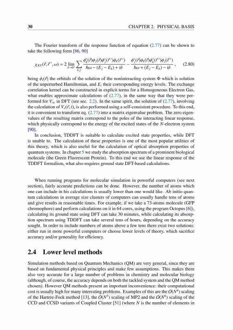
30 CHAPTER 2. PHYSICAL BASIS
The Fourier transform of the response function of equation (2.77) can be shown totake the following form [86, 90]
χKS (~r,~r ′, ω) = 2 limδ→0+
∑k, j
φ∗k(~r)φ j(~r)φ∗j(~r′)φk(~r ′)
~ω − (E j − Ek) + iδ−φ∗j(~r)φk(~r)φ∗k(~r ′)φ j(~r ′)
~ω + (E j − Ek) − iδ, (2.80)
being φi(~r) the orbitals of the solution of the noninteracting system Φ which is solutionof the unperturbed Hamiltonian, and Ei their corresponding energy levels. The exchangecorrelation kernel can be constructed in explicit terms for a Homogeneous Electron Gas,what enables approximate calculations of (2.77), in the same way that they were per-formed for Vxc in DFT (see sec. 2.2). In the same spirit, the solution of (2.77), involvingthe calculation of Vs(~r, t), is also performed using a self-consistent procedure. To this end,it is convenient to transform eq. (2.77) into a matrix eigenvalue problem. The zero eigen-values of the resulting matrix correspond to the poles of the interacting linear response,which physically correspond to the energy of the excited states of the N-electron system[90].
In conclusion, TDDFT is suitable to calculate excited state properties, while DFTis unable to. The calculation of these properties is one of the most popular utilities ofthis theory, which is also useful for the calculation of optical absorption properties ofquantum systems. In chapter 5 we study the absorption spectrum of a prominent biologicalmolecule (the Green Fluorescent Protein). To this end we use the linear response of theTDDFT formalism, what also requires ground state DFT-based calculations.
When running programs for molecular simulation in powerful computers (see nextsection), fairly accurate predictions can be done. However, the number of atoms whichone can include in his calculations is usually lower than one would like. Ab initio quan-tum calculations in average size clusters of computers can usually handle tens of atomsand give results in reasonable times. For example, if we take a 73-atoms molecule (GFPchromophore) and perform calculations on it in 64 cores, using the program Octopus [6]),calculating its ground state using DFT can take 30 minutes, while calculating its absorp-tion spectrum using TDDFT can take several tens of hours, depending on the accuracysought. In order to include numbers of atoms above a few tens there exist two solutions:either run in more powerful computers or choose lower levels of theory, which sacrificeaccuracy and/or generality for efficiency.
2.4 Lower level methodsSimulation methods based on Quantum Mechanics (QM) are very general, since they arebased on fundamental physical principles and make few assumptions. This makes themalso very accurate for a large number of problems in chemistry and molecular biology(although, of course, the accuracy depends on both the tackled system and the QM methodchosen). However QM methods present an important inconvenience: their computationalcost is usually high for many interesting problems. Examples of this are the O(N4) scalingof the Hartree-Fock method [13], the O(N5) scaling of MP2 and the O(N6) scaling of theCCD and CCSD variants of Coupled Cluster [51] (where N is the number of elements in

2.4. LOWER LEVEL METHODS 31
the basis set) the cubic scaling of some real-space DFT codes like Octopus [6] with thenumber of mesh points16. Present computational limitations together with such scalingsmake many biological systems of interest cannot be tackled by using Quantum Chemistrymethods like the mentioned ones.
To treat systems of large sizes, other lower levels methods have been developed thattypically sacrifice accuracy and/or generality if compared to QM methods for the sake ofgreater efficiency. Among these levels of theory are Molecular Mechanics (MM), Quan-tum Mechanics/Molecular Mechanics (QM/MM) and semiempirical methods. In this sec-tion, we provide a brief summary of the basic ideas behind these three methods.
Semiempirical methods [13, 51, 91] are variations of QM methods which avoid thecalculation of the most computationally expensive terms of higher level methods by re-placing them by known functions, which depend on parameters which are fitted to matchexperimental results or more accurate theoretical calculations. Basic versions of HFinvolve integrals depending on four atomic orbitals, thus resulting in an O(N4) scal-ing. Semiempirical HF-based methods17 neglect the integrals depending on four orbitals(among others), and modify the expressions of the non-neglected integrals to compensatethat approximation. To this end, different parameters are to be used into the non-neglectedintegrals. The value of these parameters and the concrete neglected integrals are distinctfor different semiempirical methods [51]. In semiempirical methods, the core orbitals arenot usually explicitly treated, since they are assumed to be sufficiently invariant not toimply chemical consequences [13], what makes calculations more efficient. Commonly,for Hydrogen atoms only s- orbitals are used, while for atoms belonging to the secondand third row of the periodic table only s- and p- orbitals are used in the semiempiricalscheme. Further explanations on the parametrization of semiempirical methods can befound in [91].
The family of methods known as Molecular Mechanics goes one step further anddescribes all the interactions between the atoms without direct reference to the electrons,but instead using known parameterized functions, known as Force Fields, as the potentialenergy dependent on the positions of the (classical) nuclei.
A typical Force Field depends on atom positions and on internal degrees of freedom(bond lengths, bond angles and dihedral angles), which can be described as follows (seefig. 2.4)18:
é Bond length: Distance between two atoms joined by a covalent bond.
é Bond angle: Angle formed by the lines of two covalent bonds that share an atom.
é Dihedral angles: In a molecule, if four atoms (say 1, 2, 3 and 4) are linked bythree covalent bonds, they define two planes, each containing two bonds. The anglebetween these planes is called dihedral angle. There are two kinds of dihedral an-gles. If bonds are 1-2, 2-3 and 3-4, the two planes are those containing atoms 1,2,3and 2,3,4, respectively. This type of angle is called principal dihedral, torsional or
16Please note that these scalings are valid for simple versions of the aforementioned methods, which maynot be the most efficient versions of them.
17Most semiempirical methods are based on the Hartree-Fock level of theory, although there existsemiempirical methods which are based on other theory levels, such as Density Functional Theory [13].
18For a more detailed discussion about the use of internal coordinates, see [92].

32 CHAPTER 2. PHYSICAL BASIS
proper dihedral . If bonds are 1-2, 2-3 and 2-4, the two planes are those containingatoms 1, 2, 3 and 1, 2, 4, respectively. This kind is called phase dihedral, harmonicor improper dihedral.
Figure 2.4: Internal coordinates. Blue lines indicate covalent bonds, while spheres representatoms. On the left side (A) we can see a bond length (d, between atoms 4 and 3), a bond angle (φ,in magenta, involving atoms 4, 3 and 2) and a principal —or proper— dihedral angle θ, in green. θis the angle between the plane determined by atoms 1, 2 and 3 and the plane determined by atoms2, 3 and 4. On the right side (B), we can distinguish a phase —or improper— dihedral angle θ,which is the angle between the plane determined by atoms 1, 2 and 3 and the plane determined byatoms 1, 2 and 4.
The expression of a typical Force Field as a function of this internal coordinates andthe Euclidean positions is a sum of simple known functions. These functions dependon many parameters, whose values are chosen so that results of experiments or higherlevel calculations are reproduced. Since there are different values for different terms ofthe potential (2.81) and for different atoms with different neighbours, FF’s can includethousands of these values [93]. For example, the partial charge in a tetrahedral Carbon isnot the same than the partial charge in a planar Carbon.
Typical (Class 1) Force Fields have the following form
V(q) = VBL(q) + VBA(q) + VPD(q) + V(q)ID + VCoul.(q) + VvdW(q) , (2.81)
where q are all the degrees of freedom of the system. The terms in (2.81) correspond tobond lengths, bond angles, proper dihedral angles, improper dihedral angles, Coulombicinteraction and van der Waals interaction, respectively. Other terms can be added to (2.81),what can increase the accuracy of simulations at the cost of a higher numerical complexity.It is worth remarking that, in order to perform simulations with Force Fields, we need toknow the connectivity of the atoms a priori, because Force Fields cannot account forbond breaking or bond formation. Class 1 Force Fields can neither account for electronicpolarizability. Other ones (polarizable Force Fields) can, but at a computational cost thatis commonly one order of magnitude higher than that of Class 1 Force Fields [13].
The evaluation of the forces associated to internal coordinates VBL, VBA, VID and VPD iscomputationally cheap, since, there are usually only three internal coordinates associatedto every atom of any molecule. As a result, the numerical complexity of these forcesis roughly proportional to the number of atoms of the system. However, the long range
2.4. LOWER LEVEL METHODS 33
terms corresponding to electrostatic and Van der Waals interactions do not present thissatisfactory property. VCoul. and VvdW are often called non-bonded terms, and calculatedonly for atoms not taking part of the same bond length, bond angle or dihedral angle[93]. These terms are pairwise, so they are expected to be harder to deal with, because(in principle) they involve Na(Na − 1)/2 evaluations, where Na is the number of atoms ofthe system. This quadratic scaling can be reduced by a number of methods (see chapter4 for a more detailed review). The electrostacic potential can be calculated, for example,using the Fast Multipole Method [94, 95], the Particle Mesh Ewald method [96], the fastFourier transform [97], the Particle-particle particle-mesh method [98] or several cutoff
methods.Force Fields have proven to be very successful when applied to biological molecules,
like peptides and proteins [99, 100], nucleic acids [101], sugars and fatty acids [93]. ForceFields can also be used in simulations of protein folding processes, which usually takefrom milliseconds to seconds to take place. Time steps required by Molecular Mechanicssimulations are usually of the order of femtoseconds (10−15 s.), what makes the even-tual simulations of protein folding processes to take over 1012 steps for typical proteins.The calculations to be performed in each step scale with the number of atoms. Thesetwo features make the total time that would be necessary for the simulation of the fold-ing of many typical proteins to exceed the current computational capabilities, even forthe most powerful supercomputers. Recently, however, a special-purpose supercomputer(the Anton supercomputer) designed for Molecular Dynamics simulations of biomolec-ular systems using Force Fields has been able to reach that limit [9] for a rather small,fast-folding protein. Molecular Mechanics is also appropriate to simulate nucleic acids.ADN and ARN are formed by only 4 distinct building blocks called nucleotides (in con-trast to proteins, which are commonly formed by 20 distinct blocks). However, ForceFields are sometimes less accurate when dealing with them. This is because nucleic acidsare quite flexible, what makes long-range interactions to have more influence on them,and dispersion forces, which are difficult to simulate, to be central for their stability [102].
Despite their successes, the application of force fields still presents some importantdrawbacks that are worth mentioning. For example, at present, there are no widely dis-tributed Force Fields which accurately model the structure of bioinorganic moleculeswithout ad hoc parameterization [103]. Force Fields have not been quite developed totreat metallic systems, what is attributable to the role of partially occupied d-orbitals inmetals, whose behaviour is hard to parametrize. Promising attempts, however, are ob-ject of current research [104]. Other recent advances have been made to build ForceFields which are accurate for non-metallic condensed matter systems, like liquid waterand molten salts [12]. Class 1 Force Fields are not polarizable, what can make theminacurate for treating metals.
Finally, to close this section, let us mention that MM and QM can be used togetherin what are called QM/MM methods (see chapter 5 for an example of their application).The idea behind QM/MM is simple. In order to deal with a large system, consisting ofmany atoms, this system is split into two regions, each being analysed using a differentlevel of the theory. The part where MM might make significant errors, or the part of thesystem which is most determinant for the quantities we want to calculate is treated usinga QM method, while the rest of the system is treated with Molecular Mechanics, which isgenerally more efficient. As mentioned, the MM part of the Hamiltonian cannot account

34 CHAPTER 2. PHYSICAL BASIS
for breaking and formation of bonds, so it is important that the part of the molecularsystem where these phenomena may take place is included in the region treated withQM19. In the framework of QM/MM, the form of the Hamiltonian is
H = HQM + HMM + HQM/MM , (2.82)
where H is the total Hamiltonian, and HQM, HMM and HQM/MM are the parts correspond-ing to the region treated with Quantum Mechanics, to the region treated with MolecularMechanics and to the interaction between both regions, respectively. HQM/MM typicallycorresponds to nonbonded interactions, including the Coulombic and van der Waals inter-actions [13].
2.5 Calculating observable quantitiesIn previous sections of this chapter, we have presented methods to calculate the potentialenergies of atoms or atomic nuclei20 whose positions are known. Since matter is not static,but in constant motion, the calculation of observable quantities of a system requires theknowledge of the force and potential energy not in only one conformation, but in many.In the rest of this section we will very briefly explain two popular methods to performsimulations of molecular systems: Molecular Dynamics (MD) and Monte Carlo (MC)simulation. We can divide a molecular simulation into two stages: 1) To get the potentialenergies of the atoms (and, if necessary, also forces and higher derivatives), and 2) Toextract physical properties from this potential. The discussions in previous sections (2.1∼ 2.4) refer to stage 1, while MD and MC methods correspond to to stage 2.
Molecular Dynamics [105] is the technique which simulates the motion of atoms bytreating nuclei as classical particles under the forces resulting from potentials calculatedby any suitable method (such as Force Fields or Density Functional Theory). In MD,time is divided into discrete steps (called time steps and with a typically constant lengthdenoted by ∆t), and the quantities of previous steps are used to predict the positions andvelocities of the atoms in subsequent ones. The specific way in which this is done isspecified by a family of algorithms called integrators. They are usually required to havethree features to reliably reproduce physical behaviour of molecules: time-reversibility,symplecticness and stability [106]. Time-reversibility is the property of an algorithm to re-trace its calculated trajectories backwards if the sign of momenta (or velocities) is changed[107]. Symplecticness is the conservation of volume in the phase space throughout thetrajectory. It is important because Hamiltonian systems are symplectic [108], what makessymplectic integrators be much more stable in the long-time than non-symplectic ones(see fig. 2.5). A numerical integrator is said to be asymptotically stable if, for a linearforce model input (satisfying d2x
dt2 = Ax, being A a matrix), the trajectories are asymp-totically bounded [106]. Keeping stability is an important requirement for integrators.Currently known high-order integrators have stability problems, and order 2 ones (i.e.,taking just second derivatives of positions) are typically used for most applications.
19In sec. 2.2 some examples were given on how DFT methods account for the formation of chemicalbonds.
20Some Quantum Chemistry methods treat explicitly only the valence electrons, while the core electronsare assumed to keep attached to the nuclei. The set of a nucleus and its attached core electrons is called ion.In cases like this, Ψ and ρ are used to calculate the forces on ions.

2.5. CALCULATING OBSERVABLE QUANTITIES 35
One of the most popular integrator is the Verlet integrator [51, 109] (the second or-der Leap-frog integrator is equivalent, and also very popular). The purpose of the basicequation of the Verlet integrator (2.83c) is to obtain the positions of a nucleus at iterationi + 1 (~ri+1) from its positions in previous steps (~ri and ~ri−1) and the force acting on it (m~ai,being m the mass of the nucleus). The propagation equation for the Verlet integration canbe derived as follows. At the i-th iteration of a MD simulation, we denote the position ofthe i-th atom with ~ri, its velocity with ~vi, its acceleration with ~ai, the time derivative of itsacceleration (i.e., the third derivative of the position) with respect to the time with ~ai, andthe time step with ∆t. Then, Taylor expansions of the position for the time steps (i − 1)and (i + 1) lead to:
~ri+1 = ~ri + ~vi∆t +~a2
(∆t)2 +~a3!
(∆t)3 + . . . , (2.83a)
~ri−1 = ~ri − ~vi∆t +~a2
(∆t)2 −~a3!
(∆t)3 + . . . , (2.83b)
~ri+1 = 2~ri − ~ri−1 + ~a(∆t)2 + O(∆t)4 , (2.83c)
where (2.83c) is merely the addition of (2.83a) and (2.83b). The error in the trajectoriesmade by this method is proportional to the fourth power of the time step (i.e., O(∆t)4).
The commonly high number of degrees of freedom involved in a MD simulation usu-ally21 makes the system chaotic (i.e., extremely nearby initial conditions span trajecto-ries diverging in time); trajectories in 6Na-dimension phase space diverge exponentially(where Na is the number of atoms of the system). Therefore, in a typical simulation it isabsolutely impossible to follow the actual physical trajectories of the real system. How-ever, although there is not a formal proof of it, MD-modelled evolution of systems tendsto follow shadow orbits. A shadow orbit is a true trajectory of a many body system thatclosely follows the numerical trajectory for a time that is long compared to the time needfor instabilities to appear [105]. Hence, the physical quantities one wants to calculatevia numerical simulation can be reliable although the simulated trajectory is not the ac-tual physical one. The success of MD predictions, confirmed by much numerical data,supports this hypothesis.
Molecular Dynamics calculations can be performed in very powerful PFlops comput-ers22 [14]. MM, using Force Fields, are mostly used when thousands of atoms are to betackled23. A recent breakthrough is the simulation of the protein BPTI in explicit waterof [16], analyzing 17,758 particles at MM level considering O(1012) steps, which is 100times more than the previous state-of-the-art. Another remarkable example is in [111],where 2.64 millions of atoms are simulated using NAMD [108], a MM program speciallydevised to deal with high numbers of atoms.
The spirit of Monte Carlo24 simulation methods is rather different to Molecular Dy-namics’. In the context of Statistical Mechanics, every conformation of a system of Na
atoms must be considered, each conformation being determined by a concrete value of its21“For essentially all systems that we study by MD simulations” [110].22I.e., computers capable of performing 1015 floating point operations per second.23Of course, this statement is valid at present; it is to be expected that both the hardware and software
capabilities will increase much in the coming years.24So called because it involves the use of random numbers [105], as those determining the fortune in
Monaco’s casino.

36 CHAPTER 2. PHYSICAL BASIS
Figure 2.5: Example of influence of symplecticness in the stability of long-time trajectories.Both figures represent the phase space of a one-dimensional harmonic oscilator. Dark regionsrepresent points occupied at any time in a 10,000-step simulation. Left: Using a symplectic in-tegrator (Euler); Right: Using a non-symplectic integrator (Runge-Kutta). The trajectory of thenon-symplectic method does not conserve the energy, while the symplectic method does, and keepsa stable orbit [108].
6Na coordinates in phase space (positions, q and momenta, p). The measured value ofany observable quantity A calculated using Classical Statistical Mechanics in the canoni-cal ensemble is given by
〈A〉 =
∫dp dq A(p,q)exp[−βH(p,q)]∫
dp dq exp[−βH(p,q)], (2.84)
where β := kBT (where kB is the Boltzmann constant and T is its temperature, and H(p,q)is the Hamiltonian of the system. In (2.84), the integration is performed over all possiblevalues of the positions and momenta.
Commonly, the Hamiltonian is an addition of the kinetic and potential energies (H =
T + V). Since the dependence of T with the momenta is quadratic, averages of functionsdepending on p can usually be performed analytically25. If momenta are integrated out,(2.84) becomes
〈A〉 =
∫dq A(q)exp[−βV(q)]∫
dq exp[−βV(q)]. (2.85)
Expression (2.85) is hardly ever analytically integrable. Therefore, the integrals in it areto be replaced by a summation with enough terms to give a good approximation for 〈A〉.Therefore, a set of conformations needs to be chosen, the Hamiltonian and the observableA are to be evaluated for every conformation in the set, and their values are to be includedin the summations for 〈A〉. However, the size of the integration space is exponential in thenumber of degrees of freedom, which precludes any simple choice for this set of confor-mations, such as a regular grid. To solve this problem, a special family of Monte Carlomethods known as importance sampling was introduced at the beginning of the modern
25The integral of the exponential of a quadratic expression of an Na-dimensional vector p involving aNa × Na positive-definite matrix A is
∫dp exp
(−(p)T Ap
)= (πNa/det A)1/2, where the superscript T means
transposed, and det denotes determinant.

2.5. CALCULATING OBSERVABLE QUANTITIES 37
computers era, being one of the best known algorithms in this family the Metropolis algo-rithm [112]. According to this method, the following steps must be performed to producea potentially infinite chain of conformations:
é From the conformation of the present step (step i), qi, to produce a proposed newone q′i , in a way that meets certain technical requirements (e.g., detailed balance)[105]
é To accept or to reject the produced conformation. (q)′ will be accepted as the con-formation of step (i + 1) if its (potential) energy is lower than that of qi: V((qi)′) ≤V(qi); If its energy is higher (V((qi)′) < V(qi)), then (q)′ will be accepted as theconformation of step (i + 1) with a probability of exp[−β(V((q)′) − V(q))].
é To store qi+1.
é To go back to the first point of this list (the new starting point will be qi+1).
The resulting chain can be used to compute (2.85) as indicated, although some compli-cated technical considerations, such as whether or not all conformations should be usedor how long must the chain be, have been deliberately omitted because they fall outsideof the scope of this account.
The high number of steps required for MD and MC simulations and the complexityof calculations for each step lead to perform the corresponding calculations in powerfulcomputers. To this end, there exist a variety of packages for molecular simulations. Somewell-known examples, such as AMBER [113] or Gromacs [114], use Force Fields forpotential energies in Molecular Dynamics. On the other hand, some others as CHARMM[115] or DESMOND [116], allow to perform Monte Carlo calculations as well. Withrespect to levels of the theory rather than Force Fields, there exist a number of codes, suchas NWChem [117] or Octopus [6], that use potential energies which are calculated usingQuantum Mechanics. Popular methods to use QM potentials in Molecular Dynamicssimulations are Car-Parrinello MD [118] and Ehrenfest MD [119].


Chapter 3
Computational aspects
In this chapter, we introduce some basic computational aspects which are related to theresearch chapters of this thesis (chapters 4 - 9). In section 3.1 we present some ideas onhow the daily work of a scientist who uses computational resources in his work can be. Insection 3.2, we present some funtamentals of High Performance Computing.
3.1 Running algorithms in real computersThe increase of existing computational capabilities has made computation to emerge asa third discipline of Science, lying midway between experimental and purely theoreticalbranches [120]. When performing molecular scientific calculations, both software devel-opers and software users should try to avoid some important issues related to methodol-ogy, which are commonly related to accuracy and execution time. We call accuracy tothe similarity between the result of a given calculation and the hypothetical result thatwould be obtained if we were able to perform the same calculation without any numericalerror. When calculating physical quantities, the accuracy26 is essential, because its lackmakes results not to be reliable. The accuracy can be lowered by many sources of errorthat exist for calculations performed in computers. For example, real numbers are usuallyrepresented in floating point notation, each number being encoded in a finite number ofbytes, usually 4 or 8. A real number is said to be represented in single precision if 4bytes (i.e., 32 bits, 32 binary figures) are used, and it is said to be represented in doubleprecision if 8 bytes are used. In the popular IEEE arithmetic, the 32 bits of a single-precision number are distributed as follows: 1 bit for the sign, 8 bits for the exponent,and 23 bits for the fraction [121]. Number e stands for the exponent, while f stands forthe fraction. Together, they represent a real number whose absolute value is 1. f × 2e (thenotation 1. f means that f is the fraction to be added to 1; for example, if the fraction is0.25, then the number to multiply by 2e —the significand— is 1.25). A simple way torepresent integer numbers in binary code is to use the first digit for the sign (0 for -, 1for +) and the n-th digit to be multiplying 2n−1. In this code, for example, the 8-digitsbinary number 01010011 = - (1 × 26 + 0 × 25 + 1 × 24 + 0 × 23 + 0 × 22 + 1 × 21 + 1 × 20
= -83). The integer number for the exponent (e) is sometimes represented in the bias26The word precision is sometimes used as a synonym of accuracy, but we prefer not to use it because,
more properly, ’precision’ means low standard deviation from a mean value, which need not be the actualsought value.

40 CHAPTER 3. COMPUTATIONAL ASPECTS
code, which is different than the one just presented. In the bias code, the number that erepresents is the number its figures represent (according to the encoding just presented)minus a given number, which commonly equals 2bit number−1. For example, in this notation0011 , 3, 0011 := 3 + (−24−1) = −5. In the coding used for the fraction part f , each fig-ure is to be multiplied by the inverse power of 2 corresponding to its place. For example,f = 0100 → f = 0 × 2−1 + 1 × 2−2 + 0 × 2−3 + 0 × 2−4 = 0.25.
The finite size of variables stored by computers implies that a finite number of binaryfigures is used to represent every number. This implies that not all the existing real num-bers, but only a subset of them, can be exactly represented in a computer. In most cases,when representing one number in a computer we are using not that very number, but theclosest number to it that the computer can represent (in a given notation). Every rationalnumber with a denominator which has a prime factor which is not a power of 2 will has aninfinite binary expansion. Let us see an example. If we are dealing with single precision,floating point, real numbers according to IEEE arithmetic, then the number 0.1 is exact inthe decimal notation, but it is periodic in binary notation. Its value is
e = 01111100 = −4; f = 1001100110011001100110011001100 . . .
We can notice that the represented single precision binary number is not exactly the num-ber we wanted to represent:
1 01111100 10011001100110011001100 =
+ 2−4(1 + 1 × 2−1 + 1 × 2−4 + 1 × 2−5 + 1 × 2−8 + 1 × 2−9 + 1 × 2−12 + 1 × 2−13 + . . .)= 0.09999999404 , 0.1 . (3.1)
Errors made in this way are called machine precision errors. If we do an operation withseveral numbers, each represented in limited precision, the errors can accumulate. Forexample, consider we want to calculate the product of two (actual) numbers aa and ba.We cannot represent them exactly in the computer, but we can only represent ar, br suchthat aa = ar + ra and ba = br + rb. If we calculate their product in the computer, we willget (a × b)r = ar × br + ea×b, being
aa × ba ' ar × br + ar × rb + br × ra . (3.2)
If we multiply many numbers, the individual errors can accumulate. Making any otheroperation or sequence of operations using real numbers can propagate errors as well. Insummary, results in a computer calculation are usually not exact, but they depend on theprecision27 (number of bytes used to represent a real number) chosen.
The order the operations are performed in an algorithm makes the machine preci-sion errors to propagate in different ways. There exist virtually an infinity of algo-rithms capable of doing some given calculation, for there exist many mathematicallyequivalent ways to do the calculations aimed to reach a desired result. When these al-gorithms are implemented to do calculations in a computer, the way in which the er-rors accumulate can be quite different. For example, if a and b are real numbers, thena/b , a × (1/b), with a slight difference. We can appreciate it in the following example.
27Do not confuse this (computer precision) with statistical precision, related to typical deviations.

3.1. RUNNING ALGORITHMS IN REAL COMPUTERS 41
Let aux1 be a double precision variable (i.e., it has about 16 decimal digits of precision),the code28
aux1=1234567891011121314150000000000.;for (i = 0; i < 220; i + +) do
aux1=aux1/1.3456789333;end for
gives a result 53.0145642653708151, while the codeaux1=1234567891011121314150000000000.;for (i = 0; i < 220; i + +) do
aux1=aux1*(1./1.3456789333);end for
results in 53.0145642653714972. Hence, both results differ in the 14th figure. This ismerely a simple example, but it can be useful to notice that every algorithm implementa-tion has its own way to propagate errors. In chapter 8 we present an example on how twomathematically equivalent algorithms result in different accuracies for the solution.
In addition to the finite precision and the differences in the algorithms, computers alsointroduce soft errors, which are defined as errors in processor execution that are due toelectrical noise or external radiation rather than design or manufacturing defects [122].
Apart from errors arisen from technological limitations, the algorithm chosen to solvea given problem has also its own sources of error. Every algorithm has its own mathemat-ical definition and is based on a given level of theory. For example, iterative algorithmsrequire an starting guess, which may lead to wrong results if it is not appropriate, and theyalso require a criterion to decide when iterations should stop. The set of equations usedto tackle a system can also be an important source of error, since every system requiresappropriate equations and appropriate input parameters. In any case, the errors in the cal-culations resulting from the theory levels are not algorithmic errors and, in this Ph. D.dissertation, we will refer to accuracy just in terms of algorithmic errors.
Apart from the accuracy, the other main limiting factor in computer simulation isthe execution time. As explained in previous sections, nowadays we do know equationswhich describe small scale phenomena quite well, but whose solution for complex sys-tems is cumbersome, and often unaffordable. The numerical complexity of the solutionof simulation problems usually increases with the size or complexity of the system tack-led. This numerical complexity can be measured with the number of required operations.Some examples of this can be
é If one wants to add N arbitrary numbers, then the number of operations requiredwill be N − 1.
é Solving a linear system of equations Ax = b, being A an N×N dense matrix, requiresof the order of N3 operations using the typical Gaussian elimination scheme (seechapter 8).
é The simplest implementations of the Hartree-Fock method to find the ground stateof the electronic Hamiltonian (see the Schrödinger equation in sec. 2.1) require
28This example is valid just in a given computer under a given programming paradigm, although it cangive an idea on how computers work.

42 CHAPTER 3. COMPUTATIONAL ASPECTS
a number of operations which is proportional to N4, being N the number of basisfunctions used (as explained in sec. 1).
é A naive approach to calculate an estimation of the partition function of a systemdepending on N coordinates, and sampling m different values for each, takes of theorder of mN operations (exponential growth).
In all these examples the size of the system is proportional to a number N, and the increaseof N leads to an increase of the numerical complexity of the solution of the problem. Sincewhen doing any calculation we want its result to be ready within a given time, systemsbeyond a given size will be unaffordable. The scaling of the methods can sometimesbe reduced by doing a number of approximations consisting of neglecting part of theinformation involved in the problem, and expecting it will not have a major influence onresults [14].
The considerations about simulation time are more complex if not running serial pro-grams, but parallel ones. Parallel programs distribute the workload in several computingthreads, each of which is run in a different computing unit. When executing a parallelprogram, it is customary to measure its efficiency with
é The total execution time (wall clock time) which is required for a given task tNc
(which is a function of the number of cores working in it Nc)
é The speedup, which is defined as the quotient S Nc := t1/tNc This is, the time that thetask would last if run in one core divided by the time it lasts when run in Nc cores.
é The quotient S Nc/Nc (sometimes called the efficiency factor)
For a given problem of constant size, the Amdahl’s Law [123] states that if p is the fractionof the problem which can be run in parallel, and therefore s := (1 − p) is the minimumfraction which must be run in serial, then the maximum speedup that can be achieved byusing Nc cores is
S maxNc
=Nc
Nc(1 − p) + p. (3.3)
This expression has an horizontal asymptote in (1 − p)−1. The speedup can be increasedby increasing the total time required by the fraction of the problem which can be run inparallel, what usually can be achieved by increasing the size of the simulated system (forexample, increasing its number of atoms). Commonly, p is not constant, but increasing asthe size of the problem increases. Let us consider a variable-size problem which requires atime of T (s+ pNα
c ) to be solved in serial. In this expression, T is the total time required forsolving the problem of a given size in serial, and the exponent α is a given positive number.If the part that can be parallelized is indeed parallelized (assuming optimal scaling in theNc computing units), the time required by the execution in parallel will be T (s + pNα−1
c ).Applying that s + p = 1 in the ratio of serial and parallel times of a variable-size problemfor 0 < α < 1, we get:
S v :=s + (1 − s)Nc
α
s + (1 − s)Nα−1c
, (3.4)
where S v means speedup factor for variable size algorithms. If α = 0 (i.e., if the problemsize does not increase with Nc) the expression above equals the Amdahl’s Law (3.3). In

3.2. SCIENTIFIC SUPERCOMPUTING 43
the limit of high Nc, eq. (3.4) becomes
S v := 1 +ps
Nα . (3.5)
In the case of α = 1 (linear scaling of the size of the problem with the number of comput-ing units solving it), the ratio of serial and parallel time is
S Gv = s + (1 − s)Nc = (1 − p) + pNc , (3.6)
for the ideal parallelization situation. Equation (3.6) is called the Gustafson’s Law [124]and states that the speedup for solving a problem can be increased by increasing the sizeof its parallelizable part.
Considerations as the ones underlying Amdahl’s and Gustafson Laws can be usefulfor the task of scientific software developers, in order to increase the efficiency of theircodes. Parallelization characteristics of algorithms, however, are commonly much harderto derive than these laws.
3.2 Scientific supercomputing
3.2.1 IntroductionAs presented in chap. 1, scientific simulations are a useful research tool. However, theyare often very costly in numerical terms, and very powerful computers are needed to han-dle the required calculations. In the last decades, computation technologies have improvedenormously, as we will see in the next sections. Currently, even the computers that canbe found in a common computer shop are capable of performing billions (109) of opera-tions per second (datum of late 2011). For scientific purposes there exist special machineswhich largely increase this performance, which is achieved both by doing every opera-tion in a extremely brief time and by having many computing units performing operationssimultaneously. The latter feature is called parallelism, and it is essential for High Per-formance Computing (HPC), also known as supercomputing. Parallelism is a challengeboth for computer architecture designers and for software developers, since data must betransferred throughout the parts of the computer in an efficient way. To this end, specificprogramming interfaces exist, among which we can highlight MPI and OpenMP [125].It is worth stressing that running a parallelizable program in Nc computing units hardlyever makes its execution Nc times faster than running it in just one. This is mainly dueto two reasons. First, most algorithms require data transfer among computing units. Thisslows the calculations down, because the devices for the information transferring amongcomputing units in a computer do work more slowly than the computing units themselves(see sec. 3.2.4). Second, typically algorithms cannot be parallelized in a complete way.Only a part of an algorithm can be shared among several computing units, while the restof it is inherently serial, or it has to be executed in a number of cores lower than theavailable number of cores (see the Amdahl’s Law in the previous section). Despite theseproblems, high performance machines have acquired a major importance in present sci-ence, since they can frequently tackle problems which are otherwise not feasible, amongother utilities.

44 CHAPTER 3. COMPUTATIONAL ASPECTS
In the next sections, we overview the field of High Performance Computing, in anattempt to give a more complete context for the research chapters (4 ∼ 9) of this dis-sertation. All these chapters propose methods for the calculation of physical quantities(simulation), and they all include calculations which were run using high performancecomputing facilities. An important part of the explanations given in this section are basedon [124].
3.2.2 Hardware basicsThe basic scheme of a single computer is simple; it is sketched in fig. 3.1. A computercontains a memory, which is a set of physical devices to store information. The memorycontains both data to use in the calculations, and coded instructions to be provided tothe control unit so that the calculations are run. The control unit controls the data fluxand the operations that are to be performed in the arithmetic-logic unit (ALU). The ALUperforms both arithmetic operations on numbers (like addition and subtraction) and logicoperations (like AND, OR, XOR, etc.) on the binary figures (bits) of the stored variables.Computers also include a clock, which operates at a given frequency (the clock frequencyor clock rate). The clock rate determines the number of maximum operations performedper second: An arithmetic or logic operation (as well as one stage an operation is dividedinto) takes at least one clock cycle. The Control Unit and the Arithmetic Logic Unit formtogether the Central Process Unit (CPU). The basic computer device also includes aninterface which enables its interaction with the human user (input/output). High perfor-mance computers are essentially formed by the accumulation of CPU’s linked in a smartway, as we will see later.
In fig. 3.1, red arrows indicate information flux. This flux can be physically handledby different devices (network). One or several CPU’s together with some communicationdevices can be set on a semiconductor thin layer with electronic circuits (i.e., on a chip),to form a processor or microprocessor.
Figure 3.1: Scheme of the basic parts of a computer [124]. The red arrows indicate informationflux.
The data moves from and towards the ALU through a memory hierarchy followingthe pattern displayed in fig. 3.2. Information can be stored in numerous devices existing

3.2. SCIENTIFIC SUPERCOMPUTING 45
Figure 3.2: Scheme of the flux ofinformation (red arrows) in a com-puter from and towards its Arith-metic Unit through a hierarchy ofmemories [124]. Cache can havemore levels (not necessarily two).Usually, the closer a device tothe Arithmetic Unit, the fastest theinformation transferring, but thelower the storing capacity (see fig.3.3). The disk, as well as even-tual external memories like tape li-braries, are not directly connectedto the CPU. Some architectures alsoinclude direct access paths whichcommunicate the registers with themain memory.
for that purpose (the memory), each having different maximum amount of bytes to store(size) and different bandwidth (maximum rate for information transfer). They also havedistinct latencies (the latency is the time offset to add for any communication). For ex-ample, if y bytes of information are to be transferred from a memory device which has alatency of l seconds, and a bandwidth of b bytes/second, then the minimal time requiredfor the information to be delivered will be t = l + y/b. Not only the different kinds ofmemory have a latency and a bandwidth, but also the network does. Latencies and band-widths have a major influence on computer’s performance. In fig. 3.2 we can see thescheme of connection of an arithmetic unit with several types of memories. Commonly,closer connections are with memories with lower latency and higher bandwidth, thoughsmaller size. A scheme of the memory hierarchy, including their present day typical sizes,bandwidths and latencies, is displayed in fig. 3.3.
Figure 3.3: Hierarchy of memories in a computer [124, 126], with typical values of their la-tency, memory size and bandwidth. The lower the delay in data transferring (latency), the higherthe bandwidth and the lower the size of the memory. Blue borders indicate elements typical insupercomputers, while black borders indicate elements which are present both in supercomputersand in personal computers. White shapes do not represent memories, but networking devices forinterconnection of nodes in supercomputers.
The information which is expected to be used immediately by the CPU is stored in its

46 CHAPTER 3. COMPUTATIONAL ASPECTS
registers, which have a very low latency, but can only store a small amount of information.At present, typical CPU’s have between 16 and 128 user-visible registers [124]. The nextlevel in the hierarchy of memories (after the registers) is the level of cache memories.There exist typically three different levels within this one, which are usually denotedwith L1, L2, L3. When the CPU needs some data, it first checks whether or not theyare stored in the cache. Efforts in circuit integration are specially aimed to increase thestorage capabilities of caches, in order to reduce the time to access the information theCPU requires.
After caches, the next level in the memory hierarchy is the main memory (which issometimes called RAM, although these acronym refers to a concrete type of technology).
The disk (hard disk drive, or HDD) has larger storage space, but higher latency andlower bandwidth. Although access to disk is the slowest if compared to acess to othermemories, it is the only memory capable of storing information permanently [84] (exceptfor external memories, such as CD-ROMs, pen drives, etc.).
The first disk memory was developed by IBM in 1956. This first device was able tostore 2 kilobits/in2, while disks manufactured today can store data at densities of 0.25Terabits/in2 [127]. In the last decades, the space of data volumes is doubling each year oreven faster [128, 129]. It is worth mentioning that the increase in disk memory capabil-ities has been boosted by the discovery of the giant magnetoresistance [130, 131]. Thisphenomenon makes it possible to manufacture MRAM memories which store information(bits) in magnetic layers [132].
The increase in memory size of devices such as caches, RAMs and disks is quiteuseful for simulation, because much information of the tackled complex systems has tobe frequently stored during the calculation process, what makes memory an importantlimiting factor for in silico scientific calculations. Data storage is reported to be a bigenergy consumer; moreover, its power intake tends to grow because storage requirementsare increasing over and over, and disks are faster and faster [133] . The low speed toaccess the information of disks is another drawback of the current technology. I/O (inputand output to disk) bandwidth has not advanced as much as storage capacity. As stated in[128]: ’In the decade 1995-2005, while capacity has grown more than 100-fold, storagebandwidth has improved only about 10-fold’.
External29 devices to store information close the hierarchy of memories. These devicescan be CD or DVD disks, USB flash drives, or different technologies. Massive storagedevices, as tape libraries (see fig. 3.4), are often used in supercomputers. Sometimes, theexpressions primary memory for registers, cache and main memory, secondary memoryfor hard disks and tertiary memory for non-local memories are used.
3.2.3 Beyond the Von Neumann paradigmThe basic computer scheme of fig. 3.1 comes from the Von Neumann paradigm, whichwas defined in the early times of computer architecture. This scheme has been kept acrosstime because new designs have been required to deal with previous software [134], which(in the beginning) was devised to be coherent with Von Neumann’s pattern. However, thisarchitecture is not optimal for many present day purposes, since it is inherently sequential[134]. The CPU can only deal with one instruction with (possibly) a single operand or
29Sometimes called non-local.

3.2. SCIENTIFIC SUPERCOMPUTING 47
Figure 3.4: Non-local tape memory at the JSC (Jülich, Germany).
a group of operands at a time (i.e., at a clock cycle). Another main drawback is the VonNeumann bottleneck, resulting from the fact that data and instructions must be continuallyprovided to the CPU, thus making inevitable to perform many time-consuming accessesto the memory. Attempts to improve the speed to perform operations continue to bedeveloped. Some of them are related to software techniques and compilers, while someother are related to the CPU machinery. Among the latter, we highlight the following ones[124]:
é Integration: Semiconductors research has boosted the miniaturization of transis-tors, enabling an exponential growth of the number of them which can be includedon a single chip (see fig. 3.5). Since the 1960s, the number of transistors that can beincluded on a semiconductor chip approximately doubles every two years. This factis know as Moore’s Law. Most transistors on a chip are used to store information inthe cache memories. Since the time required to access cache’s information is muchlower than that of other memories (see fig. 3.3), this integration of transistors makescomputations faster. Processors released in the years 2008-2011 have typically ofthe order of 109 transistors, and their surface is of the order of squared centimeters.
é Clock rate increase: Until recent times, the clock frequency has followed its own’Moore’s Law’, growing exponentially, although at a lower rate than the numberof transistors per chip (increasing about 1.75 times every two years). This growthhas recently (c. 2006) collapsed [129] (see fig. 3.5) because the higher the clockrate, the larger the power consumption, which scales with the cube of the clock rate[134, 135], and higher rates would require cumbersome cooling systems.
é Pipelining: It consists of making different functional parts of the CPU to performdifferent stages of a more complex task. For example, assume an instruction con-sists of 5 stages, and each has to be performed by a different part of the CPU afterthe previous stage has been completed. If every stage takes one clock cycle, then toperform the whole instruction would require 5 cycles. But if every part is giving oneresult per clock cycle, up to 5 instructions could be run every 5 cycles (the optimalperformance for pipelining is one instruction per cycle). Splitting instructions intomany stages can therefore increase the speed of calculations. Pipelining enables

48 CHAPTER 3. COMPUTATIONAL ASPECTS
greater clock rates, but these are limited by the power consumption. Modern pro-cessors are strongly pipelined, and some of them divide basic instructions into over30 stages.
é Superscalarity: It is the capability of CPU’s to provide more than one result perclock cycle. It is partly based on pipelining, but not limited to it. Other features alsocontribute to superscalarity. For example, if some parts of the CPU are redundant,further parallelization can be attained. The CPU design can also be tuned so thatmultiple instructions (3 to 6 nowadays) can be fetched and decoded at a time. Theavailability of very fast caches, which can perform over one load or store operationper cycle, also improves superescalarity. The compiler should take advantage onthe superscalarity features of a computer.
é Multicore architecture for processors: In order to overcome the limitations givenby the sequential nature of the Von Neumann model, a powerful solution is to in-clude not only one, but several CPU’s (cores) per socket30, thus forming multicoreprocessors. This new paradigm uses the additional available transistors to put newcomputation units to work, rather than to try to make a single core faster [129].Multicore solutions are more and more employed in common PC’s. They are also acommon solution to circumvent the problem of the high energy consumption in su-percomputers [135, 136], since the performance of the processor can be increasedeven when reducing the clock rate. The many core processor architecture sharesthe increasing available transistors (being doubled every two years according toMoore’s Law) among the cores. The inclusion of more cores, however, also car-ries inconveniences, because the growth of the number of cores per chip impliesa reduction in both the main memory bandwidth and the cache size available foreach core. Another inconvenience of multicore architecture is that the presence ofmany CPU’s simultaneously solving the same problem implies that the code of theprograms should be devised to provide them with the appropriate parallel instruc-tions, which they should execute at the same time. The recent trend to use multicoreprocessors can be appreciated in fig. 3.5. It is worth remarking that, while pipelin-ing and superscalarity are perfectly compatible with the Von Neumann model, themulticore architecture is not. It is a modification of that paradigm, which entailsnew rules for the flow of information and the way in which the computer acts on it.The multiple cores of a processor can either lie on the same chip or not, but theylie on the same socket. Some examples of multicore schemes are displayed in fig.3.6. Typical PC’s have a single socket, while servers commonly content two to foursockets, all sharing the same main memory. Big parallel computers (see sec. 3.2.4)commonly contain many sockets.
é SIMD instructions: SIMD (single instruction multiple data) instructions enabledata parallelism by performing arithmetic operations not on a single number, buton a vector of them. The supercomputers of the 1980s and early 1990s were basedon this principle (although at a much larger scale) and they were called vector ma-chines. Although big vector machines are rare at present, its principle can still beuseful for other computers.
30A socket is the physical package where the multiple cores are joined. See figure 3.8.

3.2. SCIENTIFIC SUPERCOMPUTING 49
é Out of order execution: If the arguments of the instructions are not available inregisters when they must be used, what can happen if the memory is too slow to keepup with processor speed, out-of-order execution can avoid idle cores by executinginstructions that appear later in the instruction stream but have their parametersavailable. The compiler, after analysing the relations among different instructions,can change its order so that some slow memory readings start earlier.
é Simplified instruction sets: Paradigms of instructions which are rather simple (asopposed to previous models) but can be executed much more quickly. The RISC(Reduced Instruction Set Computer) paradigm was adopted during the eighties, re-sulting in efficiency increases.
Figure 3.5: Evolution in time of the number of transistors per chip (blue), clock rate (red)and number of cores per processor (purple). It can be appreciated that during the last years theclock rate has collapsed, while multicore solutions have started to be implemented. The number oftransistors grows exponentially at a steady rate, making Moore’s Law to be still satisfied (Courtesyof J. Dongarra; data from [134])
The trends in the evolution of the degree of integration of processors, their clock ratesand their numbers of cores are displayed in fig. 3.5. We could say that the time of steadygrowth of single-processor performance seems to be over [129], what has spurred thesemiconductors industry to start a transition from sequential to parallel computers. Theintroduction of multicore processors in 2004 (see purple line in fig. 3.5) marked the endof a 30-year period during which sequential computer performance increased from a 40%to a 50% yearly. The trends displayed in fig. 3.5 have lead to a reinterpretation of Moore’sLaw. In words of Jack Dongarra (coordinator of the top500 project): ’The number of coresper chip doubles every 2 year, while clock speed decreases (not increases). The numberof threads31 of execution doubles every 2 years’. This increase in the number of threads
31Parallel work lines.

50 CHAPTER 3. COMPUTATIONAL ASPECTS
Figure 3.6: Two possible schemes for a multicore processor. A) Hexa-core processor chip withseparate L1 caches, shared L2 caches for pairs of neighbouring cores and a shared L3 cache for allcores; B) Quad-core processor chip with separate L1 and L2, but shared L3 cache [124].
results from both the multi-core solutions and from the hardware modifications whichenable CPU’s to work in other tasks when one executing thread is stalled (for example,waiting for data) [84]. These capabilities increase computer performance, but requirethe software to be well suited to the hardware to reach maximum performance. Althougheventual physical limitations for technologies might make the thread increase trend stop inthe next years, important advances are being achieved in the direction of core integration.Intel has recently presented a prototype research chip which implements 80 simple cores,each containing two programmable floating point engines. This is the maximum singlechip integration to date, and reaches TFLOPS performance32 [14].
3.2.4 Parallel computersAs stated above, the idea behind most powerful computers nowadays is the use of manycores (which globally contain many CPU’s). A given program is divided into severalexecution lines (threads) which are simultaneously run in the different cores. Therefore,these cores solve the problem in a cooperative way. The number of cores used by a super-computer is increasing over and over in time. The definition of ’supercomputer’ or ’highperformance computer’ is rather arbitrary, because these expressions refer to computerswhich are much more powerful than common computers. Because of the technologicaladvances, it is said that today’s supercomputers are tomorrow’s PC’s (see fig. 3.15; sincea nowadays laptop is capable of doing about 1010 operations per second, it is as powerfulas a supercomputer was 14 years ago). The use of standard computer components to buildsupercomputers (the so-called commodity clusters) has made these high performance ma-chines accessible for many research groups throughout the world.
We call a parallel computer to a collection of connected cores lying in different nodes,which are connected by networks. The cores of an operating parallel computer work si-multaneously in a cooperative manner. A parallel computer is formed following a schemesuch as the one displayed in fig. 3.7. It can be decomposed into four levels: cores, proces-
32http://software.intel.com/en-us/articles/developing-for-terascale-on-a-chip-first-article-in-the-series/?wapkw=%28terascale%29

3.2. SCIENTIFIC SUPERCOMPUTING 51
Figure 3.7: Scheme of a parallel computer. It can be divided into four levels (core, processor,node and parallel computer itself). Each core contains a CPU, the basic computing unit.
sors, nodes and the parallel computer itself. Components inside a given level have distinctfeatures (e.g., bandwidth, latency, etc.) when communicating with other components in-side or outside its own module (e.g., a core communicating with one core in the sameprocessor will do it much more rapidly than with a core lying in other processor). We cansummarize the four levels of a parallel computer as follows33:
é Core: It contains one control unit, and one or several arithmetic-logic units (andtherefore one CPU). For example, cores devised under the Intel Core microarchi-tecture have three ALU’s [137]. A core can run one or several execution threadssimultaneously.
é Processor: Integrated circuit which contains one or several cores and is lying onone semiconductor layer. One or several processors are inserted in one socket34. Asocket (see fig. 3.8-b) provides a processor with physical anchoring and electricalconnection to the motherboard.
é Node: Set of processors which share a common main memory, and commonly alsoshare other resources, such as a hard disk drive or a network connection. It usu-ally consists of one motherboard where there are several sockets (although in somecases, the so-called twin motherboards, two different sets of processors joined totwo different main memories can lie on one motherboard). Communication amongprocessors in a given node is rather fast, and is provided by buses.
é Parallel computer: It comprises all nodes and the communications among them,which are provided by networks such as Infiniband or Gigabit Ethernet.
In fig. 3.8, images corresponding to the different levels enumerated above are dis-played. A) displays a processor, which contains two cores (each containing several con-trol and arithmetic-logic units). B) Displays a socket, where the processor is inserted and
33The following definitions are commonly accepted, but not universal at all. In the field of computerarchitecture there is some confusion with the nomenclature.
34The names of components are sometimes conflicting in this context. Some authors call a processorwhat we call a core, and a multi-core processor what we call merely a processor (containing several cores).

52 CHAPTER 3. COMPUTATIONAL ASPECTS
Figure 3.8: Examples of the constituents of a typical parallel computer. A) Processor (Dual-CoreAthlon 64x2 - 6400plus); B) Socket (Intel Socket 370); C) Node (the image corresponds to themotherboard of a node of the Juropa cluster at the JSC, lacking the Hard Disk); D) Cluster (theimage corresponds to parallel computers at the JSC, Jülich, Germany). Image C) is a courtesy ofJ. Alberdi. Images A) and B), Copyright (c) 2011 Pablo García Risueño. Permission is grantedto copy, distribute and/or modify these images under the terms of the GNU Free DocumentationLicense, Version 1.2 or any later version published by the Free Software Foundation; with noInvariant Sections, no Front-Cover Texts, and no Back-Cover Texts. A copy of the license can befound in http://www.gnu.org/licenses/fdl-1.2.html.
anchored to a motherboard. A motherboard (C), together with devices joined to it, form anode. Several nodes linked by interconnection networks form a parallel computer (D).
Networks connecting the constituent of a parallel computer have a critical importancefor the parallel performance of applications in it. This is because data transferring typ-ically is the dominant performance-limiting factor in scientific code [124]. The mostimportant network characteristics that need to be taken into account in order to produceefficient parallel code are its network topology (the way the nodes are connected) and itsnetwork bandwidth and latency (see fig. 3.3). These features have an important influenceon the performance of the parallel computer. Examples of common topologies are ring,grid, torus in 2 or 3 dimensions or tree [84].
3.2. SCIENTIFIC SUPERCOMPUTING 53
We will now describe briefly various types of existing parallel supercomputers. Wewill first introduce the essentials of computer parallel computers, and then some funda-mentals of other devices, like GPU’s, special-purpose computers and heterocomputers,and of other types of computation, like the cloud computing and grid computing.
Parallel computers are commonly classified into two paradigms: shared memory anddistributed memory. The latter are also known as clusters. Both operate under the MIMDparadigm, i.e., multiple instructions are given to multiple cores, which deal with multipleinput variables (data). Other systems35, like GPU’s, vector machines or microprocessorsusing SIMD protocols (explained in sec. 3.2.2) follow the SIMD paradigm, executing asingle instruction on a set of multiple data. A shared memory parallel computer is defined[124] as a system in which a number of CPU’s operate in a common shared physicaladdress space. Important versions of this paradigm are:
é UMA (uniform memory address): The access time of all processors for the mainmemory is (essentially) the same. This is attained with communication deviceshaving the same latency and bandwidth.
é ccNUMA (cache-coherent Non-uniform Memory Access): The main memory isphysically distributed across the various processors, but the circuits (logics) of themachine make this set of main memories to appear as only one large memory, sothe access to different parts is done using global memory addresses. The accesstime is different for different processors and different parts of the memory, as in adistributed memory computer.
The scheme of the UMA paradigm can be found in fig. 3.9. In UMA architectures,a device called chipset controls the information flux between the main memory and thecores. The simplest example of UMA is the dual core machinery, that recently has becomevery popular [14]. The complexity of the circuits required to keep uniform the access timemakes that, at present, the largest UMA systems with scalable bandwidth (the NEC SX-9vector nodes) have sixteen sockets [124].
Typical patterns of shared-memory ccNUMA machines are displayed in figures 3.10and 3.11. A ccNUMA computer consists of several local domains, whose memories arelocally connected (each local domain being basicly a UMA). The memories of differentlocal domains are communicated via so called coherent links. This architecture is appro-priate for large shared memory machines, but is more often used to build small 2 or 4socket nodes in supercomputers.
An architecture which is more widely used to build large supercomputers (up to thou-sands of cores) is the one whose scheme appears in fig. 3.11. Each processor socket isconnected to a communication interface (S), that provides memory access to the propri-etary NUMALink network. The NUMALink network uses routers (R) for connectionswith nonlocal units. The asymmetry of this design makes the access times very variablefor different processors and different memory positions. ccNUMA machines also havethe drawback that two or more different processors may try to access the information at agiven memory position simultaneously, and thus they would compete for its resources. Inaddition, the input/output human interface is connected with only one local domain.
35Please note that the classifications presented in this chapter not universal.
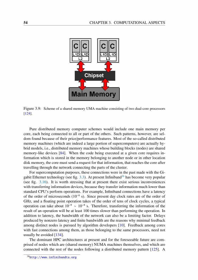
54 CHAPTER 3. COMPUTATIONAL ASPECTS
Figure 3.9: Scheme of a shared memory UMA machine consisting of two dual-core processors[124].
Pure distributed memory computer schemes would include one main memory percore, each being connected to all or part of the others. Such patterns, however, are sel-dom found because of their price/performance features. Most of the so-called distributedmemory machines (which are indeed a large portion of supercomputers) are actually hy-brid models, i.e., distributed memory machines whose building blocks (nodes) are sharedmemory-like devices [84]. When the code being executed at a given core requires in-formation which is stored in the memory belonging to another node or in other locationdisk memory, the core must send a request for that information, that reaches the core aftertravelling through the network connecting the parts of the cluster.
For supercomputation purposes, these connections were in the past made with the Gi-gabit Ethernet technology (see fig. 3.3). At present Infiniband36 has become very popular(see fig. 3.16). It is worth stressing that at present there exist serious inconvenienceswith transferring information devices, because they transfer information much lower thanstandard CPU’s perform operations. For example, Infiniband connections have a latencyof the order of microseconds (10−6 s). Since present day clock rates are of the order ofGHz, and a floating point operation takes of the order of tens of clock cycles, a typicaloperation can take about 10−9 ∼ 10−8 s. Therefore, transferring the information of theresult of an operation will be at least 100 times slower than performing the operation. Inaddition to latency, the bandwidth of the network can also be a limiting factor. Delaysproduced by nonzero latency and finite bandwidth are the reasons why minimal feedbackamong distinct nodes is pursued by algorithm developers [10]. Feedback among coreswith fast connections among them, as those belonging to the same processors, need notusually be avoided [134].
The dominant HPC architectures at present and for the foreseeable future are com-prised of nodes which are (shared memory) NUMA machines themselves, and which areconnected with the rest of the nodes following a distributed memory pattern [125]. A
36http://www.infinibandta.org

3.2. SCIENTIFIC SUPERCOMPUTING 55
Figure 3.10: Pattern of a ccNUMA system with two locality domains and eight cores. Red arrowsindicate information flux. The information is managed by a memory interface. Memory interfacesare connected via coherent links (for example, the central red arrow in this picture) [124].
Figure 3.11: A ccNUMA system with four locality domains, each comprising one socket withtwo cores. Each socket is linked to a communication interface S, and the traffic of information ismanaged by some routers R [124].

56 CHAPTER 3. COMPUTATIONAL ASPECTS
Figure 3.12: Pattern of a distributed memory computer. Red lines indicate information flux[124].
Figure 3.13: The panel of an Infiniband switch. Infiniband is a high-performance network systemwhich is present in many present supercomputers. Copyright (c) of this image: 2011 Pablo GarcíaRisueño. Permission is granted to copy, distribute and/or modify these images under the termsof the GNU Free Documentation License, Version 1.2 or any later version published by the FreeSoftware Foundation; with no Invariant Sections, no Front-Cover Texts, and no Back-Cover Texts.A copy of the license can be found in http://www.gnu.org/licenses/fdl-1.2.html
popular architecture of distributed memory computers is IBM’s Blue Gene (see fig. 3.14).In Blue Gene [138], processors lie in the vertices of a cubic grid. Each processor is com-municated with its six nearest neighbours in a 3D torus topology (the last processor, inthe border of the grid, is linked with the first one, in all three directions).
If a problem is to be solved in a cooperative manner by the various cores of a cluster,the code to be executed must be written so that the workload is shared among them. TheMPI protocol [139] is appropriate for writing codes that run in parallel in distributed mem-ory machines, being also valid for shared memory machines. The increasing popularityof MPI at present comes from its simplicity and its availability of standard libraries. Theparallelizations of many quantum simulation programs are based on MPI, although otherprograms parallelization paradigms are also used [84]. Despite its remarkable advantages,the MPI paradigm has an important drawback. Information transferring between two par-allel threads requires both of them to reach a synchronization, i.e., one must execute the

3.2. SCIENTIFIC SUPERCOMPUTING 57
Figure 3.14: The cluster supercomputer Jugene (IBM Blue Gene / P technology), in the JSC(Jülich, Germany) in Sept. 2010. In that moment, it consisted of 294,912 cores, what made it themost powerful computer in Europe, and the fifth most powerful computer in the world.
instruction for sending information —MPI_SEND— and the other one must execute theinstruction for receiving it —MPI_RECV—. In this way, the sender core will be idle untilits information is be received. The limitations of the MPI scheme can be overcome byproviding facilities for a process to access data of another process without that process’its direct participation [84]. Performance in shared memory machines can be increased byusing the OpenMP interface. Since most supercomputers have hybrid shared-distributedmemory architectures, mixed use of different programming codes, including both MPIand OpenMP is advisable [125]. However, many programmers use just MPI, for the sakeof simplicity in their codes.
3.2.5 Hybrid and heterogeneous models
A supercomputer can either be formed by the repetition of processors of the same kind, orby different ones, such as general purpose processors, graphics processing units or special-purpose chips, among others. In the former case, the architecture is called homogeneous,while in the latter case, it is called heterogeneous [140]. Heterogeneous machines canhave advantages with respect to homogeneous machines in power consumption, efficiencyof data transfer and parallel speedup. The Cray supercomputers37 are examples of hetero-geneous machines, which get high performance by using different kinds of processorswithin the same cluster computer.
Using graphics processing units (GPU’s [141]) as a part of (heterogeneous) clustersis a more and more popular solution. GPU’s were originally devised to perform fastcalculations on data for creating images. However, in recent times, they have becomecelebrated in the context of supercomputing. This is because they are capable of treating
37http://www.cray.com

58 CHAPTER 3. COMPUTATIONAL ASPECTS
much data (vectors of data, rather than single variables) simultaneously. A GPU canperform some given tasks several orders of magnitude faster than a CPU. For example,in some problems of data analysis, GPU’s performance can gain about a factor of 200with respect to CPU’s performance38. For general purpose computation issues, GPU’scan either be included in motherboards together with CPU’s, or a different type of devices(GPGPU’s39 [136]) can be produced that can work without a CPU. Full clusters can bebuilt on GPGPU’s instead of CPU’s. As a sign of the current success of GPU-basedsolutions, it can be noticed that four out of the ten most powerful supercomputers (in thelist of top500 of June 2011) do include GPU’s.
A different kind of supercomputing facility is the one formed by the special purposecomputers. These machines cannot deal with a very broad range of different tasks, as thegeneral purpose computers (PC’s, laptops, most supercomputers, etc.) can do. Instead,they are devised to execute a limited set of algorithms, but with a great efficiency. An ex-ample of a special purpose computer is Anton40, which is dedicated to protein MolecularDynamics. Anton was able to run a simulation corresponding to 1 ms (in a huge numberof steps, since ∆t is of the order of fs in proteins), realizing the hard task of predictingthe folding of a protein [9, 142]. Other examples of special purpose computers are Janus[143], which is used for simulation of spin glasses, and GRAPE-6 [144], for astronomy.
Figure 3.15: Evolution of computational capabilities: purple line: Aggregated power of all 500most powerful computers in the world, according to the top500 list; blue line: most powerfulcomputer on the world, according to the top500 list; orange line: 500th most powerful computeron the world. Notice that the vertical axis is logarithmic. Source: top500 (www.top500.org).
Fig. 3.5 and some of the subjects discussed so far can give us an idea of the evolu-tion of computational capabilities of modern computers, which grow very rapidly, in anexponential way. In order to quantify this evolution, twice a year a list of the 500 mostpowerful computers on the world, the top500 list, is released. In order to measure theefficiency of computers, a benchmark (the HPLINPACK benchmark [145]) is run. Theessential task of the HPLINPACK benchmarks is to solve a linear system Ax = b whosecoordinate matrix A is dense (i.e., contains no null entries) with partial pivoting (see chap.
38http://www.hpcwire.com/hpcwire/2011-03-29/comparing_gpus_and_cpus.html39General Purpose Graphic Processing Units.40www.deshawresearch.com

3.2. SCIENTIFIC SUPERCOMPUTING 59
Figure 3.16: Evolution of the performance of the twenty most powerful computers on the worldduring the decade 2001-2010. The names on the left hand side correspond to most powerfulcomputers on the January 2010 top500 list. (Courtesy of J. Dongarra).
8). Performance is measured in number of floating point operations per second (FLOPS)that the machine is able to perform. It is worth remarking that special purpose computerscan hardly appear on the top500 list, because it is essential to run the HPLINPACK bench-mark to appear in it, and many special purpose computers are not capable of doing it. Infig. 3.15 we can appreciate that the exponential increase of supercomputing performanceof the machines in the top500 list, both for individual supercomputers (the most powerfulone, and the one in the 500 position, appearing in the figure) and for the aggregated powerof all computers on the list. From 1993 to 2009, the computing power of the collectionof all 500 most powerful computers on the world followed its own ’Moore’s Law’, sinceit increased about 1.9 times per year (almost twice as fast as the increase in integrationpredicted by Moore’s Law). By comparing charts 3.5 and 3.15, we can appreciate that thetrends in chip integration, clock rate and number of cores per processor and the power ofhigh performance computers are closely related. In fig. 3.16, we can see the evolution ofthe 20 most powerful computers during the last decade. The vertical axis of this graphis not logarithmic, so the dramatic increase can be noticed in a more clear manner. Infig. 3.17, some features of the top500 computers are summarized. Chart A shows thenumber of cores high performance computers consist of. Chart B quantifies somethingwe mentioned earlier in this section, that vector computers are no longer popular, andmost modern computers are scalar (i.e., every CPU deals with an scalar variable at a time,not with a vector containing many values simultaneously). Chart C gives an idea of thecomputer power distributed by countries. Finally, chart D gives a notion on the network
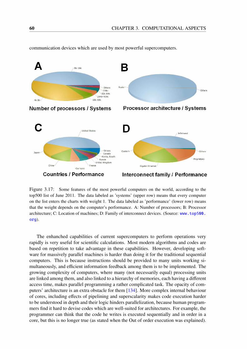
60 CHAPTER 3. COMPUTATIONAL ASPECTS
communication devices which are used by most powerful supercomputers.
Figure 3.17: Some features of the most powerful computers on the world, according to thetop500 list of June 2011. The data labeled as ’systems’ (upper row) means that every computeron the list enters the charts with weight 1. The data labeled as ’performance’ (lower row) meansthat the weight depends on the computer’s performance. A: Number of processors; B: Processorarchitecture; C: Location of machines; D: Family of interconnect devices. (Source: www.top500.org).
The enhanched capabilities of current supercomputers to perform operations veryrapidly is very useful for scientific calculations. Most modern algorithms and codes arebased on repetition to take advantage in these capabilities. However, developing soft-ware for massively parallel machines is harder than doing it for the traditional sequentialcomputers. This is because instructions should be provided to many units working si-multaneously, and efficient information feedback among them is to be implemented. Thegrowing complexity of computers, where many (not necessarily equal) processing unitsare linked among them, and also linked to a hierarchy of memories, each having a differentaccess time, makes parallel programming a rather complicated task. The opacity of com-puters’ architecture is an extra obstacle for them [134]. More complex internal behaviourof cores, including effects of pipelining and superscalarity makes code execution harderto be understood in depth and their logic hinders parallelization, because human program-mers find it hard to devise codes which are well-suited for architectures. For example, theprogrammer can think that the code he writes is executed sequentially and in order in acore, but this is no longer true (as stated when the Out of order execution was explained).

3.2. SCIENTIFIC SUPERCOMPUTING 61
Programmer is helped by modern compilers, which include several levels of optimiza-tion, what can do more efficient mapping in data transferring and result in large efficiencyimprovements. In order to devise more efficient software codes, tracing and profilingsoftware tools can be very useful [146]. Moore’s Law is said to have enabled cheaper(more efficient) execution of programs, but at a higher cost of developing new programs,by reason of the increasing complexity of computers [129]. In words of J. Dongarra, ’Forthe last decade or more, the research investment strategy has been overwhelmingly biasedin favor of hardware. This strategy needs to be rebalanced, since barriers to progress areincreasingly on the software side. Moreover, the return on investment is more favorableto software. Hardware has a half-life measured in years, while software has a half-lifemeasured in decades. Unfortunately, we don’t have a Moore’s Law for software, algo-rithms and applications’. This does not mean that the seek of efficient algorithms has notbeen successful (see chapter 4), but that modern algorithms and programs should be well-suited to current machine component features and computer architectures (an example ofthis adaptation can be found in [14], where the efficiency is increased by means as op-timizations of the transfer of data). Indeed, smart software parallelization schemes, alsoincluding new paradigms, can be the only tool to improve supercomputers’ performancein an eventual framework of exhausting of hardware capabilities increase [134].
Machines supporting High Performance Computing have to brave an important ob-stacle since some years ago: the significant rise of power consumption. The increase ofclock rates has boosted power dissipation [124], because the power consumed by a corescales with the cube of its clock rate [135]. This is attributable to the fact that the poweris proportional to the square of the voltage multiplied by the frequency, but the voltageitself is proportional to the clock frequency. Power dissipation generates heat, what isan important drawback because semiconductor materials in computers require not veryhigh temperatures in order to work properly. To this end, cooling systems must be imple-mented. 1980s computers did not need heat sinks; the heat sinks used in the nineties wereof moderate size; today’s cooling systems are very big. In PC’s and laptops air coolingsystems (fans) are usually enough, but in supercomputers water-based cooling systemsmay be mandatory in a nearby future [134]. The work of cooling systems entails seri-ous power consumptions which must be added to that resulting from processors’ work.As a result of these high power needs, the budget for electrical energy of the computingfacilities of a research group may be easily exceeded. As an example [147], a 16 coreprocessor with every core consuming an average of 20 Watts will lead to 320 Watts totalpower when all cores are active, what will have a non-negligible economic cost. Anotherexample is given by Amazon.com [148]. The energy bill of its data centers costs about the42% of the total budget of the center (the cooling system consuming more energy than theoperation of CPU’s). Many ways to reduce the impact of excessive power consumptionare being proposed [149, 150]. Architectures for many core machines should be carefullydevised to minimize it. A possible solution is to simplify processor designs. Using largercaches is another option, although there is a limit beyond which a larger cache will not payoff any more in terms of performance, due to bandwidth limitations. Multicore processorsare the solution which most present computer manufacturers prefer [124].

62 CHAPTER 3. COMPUTATIONAL ASPECTS
3.2.6 Distributed computing
Data of the top500 refers to well localized large supercomputers (like the one displayedin fig. 3.14). However, in recent times, other solutions for HPC, such as grid computing,cloud computing and volunteer computing, have become very popular. These three moremodern ways of computing are said to be ways of distributed computing. Distributedcomputing is based on the concept of doing high performance calculations using geo-graphically distant machines, what has been enabled with the advent of the internet andhigh speed networks. Computers participating in a given problem can lie thousands ofkilometers away from each other, but they can share information through the internet.
Grid computing [151] uses geographically distant nodes to solve a given problem si-multaneously in a cooperative way. Grid computing capabilities are usually managed bya given organization, and the computational resources (mediated by physical machinery)which supports calculation are contributed by different supporting institutions and organi-zations, which can be companies, research groups, laboratories, universities, etc. A man-agement committee distributes the computational capabilities at every moment among therequests of different groups of users. The groups of people taking part in grid computingprojects for solving problems are usually called virtual organizations, since these groupsare frequently heterogeneous, being formed by many people from different organizationswhich are geographically distributed. The essential aspect of a virtual organization is thatit is formed for a specific project. Virtual organizations can act either as producers or con-sumers of resources (or both). Various virtual organizations involved in a grid computingproject are mutually accountable; i.e., if one misbehaves, the others can cease sharingresources with it. Since many computer cores throughout the world are working together,much computing power can be accumulated, what enables solving many problems whosesolution may not be feasible even in the most powerful supercomputing clusters. This gen-erates vast amounts of data, what spurs the creation of large collective databases [128].Large grid computer facilities are often used by big numbers of users, what helps to matchthe demand of the computational resources with their availability.
It is also worth noticing that grid computing projects commonly operate under open-source software standards, which eases the development of software applications and thecooperation among groups. A popular software package to manage grids is the GlobusToolkit, including the GRAM software as a tool for the users. As well as cluster comput-ers, grid facilities frequently run in Linux operating systems.
Grid computing has been successful in numerous research fields, like drug design,biomolecular simulation, engineering and computation for industry, Chemistry, Geology(e.g. earthquake simulations) or meteorology [151, 152]. It also plays an important rolein Particle Physics. For example, the Large Hadron Collider of the CERN sends hugeamounts of experimental data to its associated grid facility (the Worldwide LHC Com-puting Grid, WLCG), so that many scientific groups throughout the world analyse them.WLCG41 involves over 140 computing centres in 35 countries, and includes several na-tional and international grid projects.
Recently, another kind of distributed computing, volunteer computing, has become auseful tool for scientific purposes. Volunteer computing consists of using the computationpower of machines which were neither devised nor purchased to use them to do scientific
41http://lcg.web.cern.ch/lcg

3.2. SCIENTIFIC SUPERCOMPUTING 63
Figure 3.18: A scheme of geographical distribution of computing nodes of the egee grid (http://www.eu-egee.org). Current grid computing projects often involve facilities in many countries.
calculations, but for daily life use. Common PC’s and laptops connected to the internet, asthose standing in millions of homes, can perform calculations to solve scientific problems.It is only necessary that the owner of the computer agrees and installs the appropriate soft-ware (this is the reason why this kind of computing is called Volunteer Computing). Asstated in [10], there are hundreds of millions of idle PC’s potentially available for usein every moment, and the majority of them are strongly underused. Moreover, whilethe complexity and the network efficiency have increased following their own Moore’sLaws, the number of computer users has increased at even a higher rate during the lastdecades, what makes the potential capabilities of volunteer computing huge [10]. Volun-teer computing has produced many remarkable scientific results in the last decade [153].Some examples of volunteer computing are the Ibercivis project42, seti@home43 —forthe search of extraterrestrial intelligent life— and folding@home44[154] —for statisticalcalculations of Molecular Dynamics trajectories for models of biological systems—. Thelast one is a particularly good example of how important scientific results can be producedwith volunteer computing in problems which are unaffordable for other HPC schemes[10]. Volunteer computing projects often rely on the BOINC open-source software45,which is also appropriate for grid computing. Although grid computing and volunteercomputing share some features, there is a key difference between them. Grid computingis commonly symmetric while volunteer computing is commonly asymmetric. I.e., in theformer, one organization can borrow resources one day, and supply them the next; in thelatter, contributors (particular computer owners) commonly just provide resources to theproject.
Distributed computing has become a powerful research tool because of its numerous
42http://www.ibercivis.net43http://setiathome.berkeley.edu44http://folding.stanford.edu45http://boinc.berkeley.edu
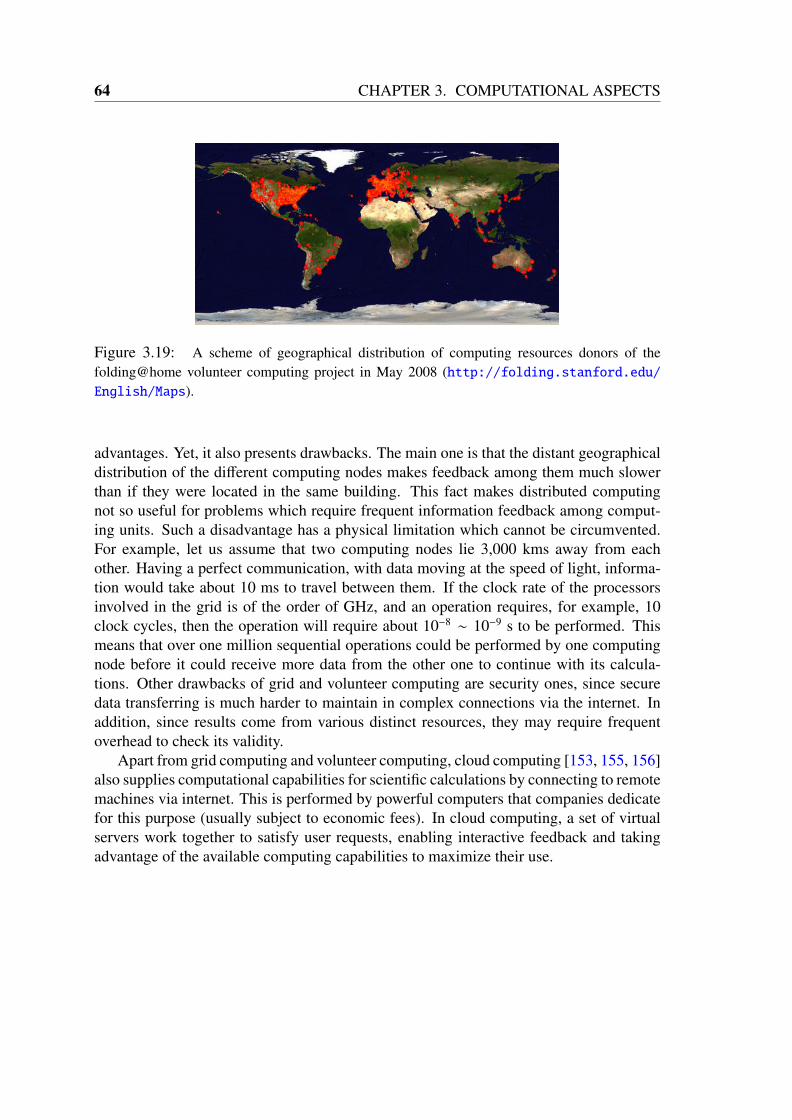
64 CHAPTER 3. COMPUTATIONAL ASPECTS
Figure 3.19: A scheme of geographical distribution of computing resources donors of thefolding@home volunteer computing project in May 2008 (http://folding.stanford.edu/English/Maps).
advantages. Yet, it also presents drawbacks. The main one is that the distant geographicaldistribution of the different computing nodes makes feedback among them much slowerthan if they were located in the same building. This fact makes distributed computingnot so useful for problems which require frequent information feedback among comput-ing units. Such a disadvantage has a physical limitation which cannot be circumvented.For example, let us assume that two computing nodes lie 3,000 kms away from eachother. Having a perfect communication, with data moving at the speed of light, informa-tion would take about 10 ms to travel between them. If the clock rate of the processorsinvolved in the grid is of the order of GHz, and an operation requires, for example, 10clock cycles, then the operation will require about 10−8 ∼ 10−9 s to be performed. Thismeans that over one million sequential operations could be performed by one computingnode before it could receive more data from the other one to continue with its calcula-tions. Other drawbacks of grid and volunteer computing are security ones, since securedata transferring is much harder to maintain in complex connections via the internet. Inaddition, since results come from various distinct resources, they may require frequentoverhead to check its validity.
Apart from grid computing and volunteer computing, cloud computing [153, 155, 156]also supplies computational capabilities for scientific calculations by connecting to remotemachines via internet. This is performed by powerful computers that companies dedicatefor this purpose (usually subject to economic fees). In cloud computing, a set of virtualservers work together to satisfy user requests, enabling interactive feedback and takingadvantage of the available computing capabilities to maximize their use.

Chapter 4
A survey of the performance of classicalpotential solvers for chargedistributions
4.1 IntroductionIn the context of Quantum Mechanics, electrons are delocalized, and so is their electricalcharge. If Ψ(x1, . . . , xN) is the wavefunction of a system of N electrons (as defined inchapter 2), then the electronic density of the system is given by (2.19d)
ρ(~r) := N∑
s1
∫dx2dx3 . . . dxN |Ψ(x1, x2, . . . , xN)|2 , (4.1)
and the charge distribution of the system equals −eρ(~r), being e the electron charge. Acharge density ρ creates an electrostatic potential V in all points ~r of the space Ω, whichis given by [157]
V(~r) =
∫Ω
d~r ′
4πε0
ρ(~r ′)|~r − ~r ′|
, (4.2)
where ε0 is the electrical permitivity of the vacuum . If the medium is not the vacuum, ε0
must be replaced by the permitivity of the medium, ε, which can be local.In 3 dimensions, eq. (4.2) is equivalent to the differential Poisson equation [158, 159]
∇2V(~r) +ρ(~r)ε0
= 0 . (4.3)
This equation can be derived from (4.2), which makes the Gauss’ Law to be satisfied∫Ω
~E(~r)d~s =1ε0
∫Vρ(~r)d~r , (4.4)
where Ω is the surface which covers volume V . The divergence theorem plus the fact thatthe electric field can be expressed as the gradient of a potential (~E(~r) = −∇V(~r)) lead to(4.3). In the case that ε is local, eq. (4.3) becomes ∇(ε(~r)∇V(~r)) + ρ(~r) = 0 [160]. If the

66 CHAPTER 4. CLASSICAL POTENTIAL SOLVERS
volume V taken in (4.4) is all the infinite space, then the boundary conditions for (4.3) canbe taken as null. However, in more realistic cases where V is finite, some given boundaryconditions must be given in order to be able to solve (4.3). Having the two forms (4.2) and(4.3) for the Hartree potential equation is useful because, while some methods are basedon the former, other rely on the latter.
The electrostatic Hartree potential appearing in (4.2) and (4.3) has a major importance,since it can be found in nearly every field of Physics and Chemistry [161]. It is speciallyimportant in Density Functional Theory and Time-Dependent Density Functional Theory,because it appears in the Kohn-Sham (2.59) and Time-Dependent Kohn-Sham equations(2.68) [54, 87, 88]. In a computational framework, the charge density ρ in (4.2) can bemodelled in several ways. Some programs [162, 163] use a set of functions as a basis,and build the density as a function of them. Other ones [6] store the information of thesystem in a grid of points. For example, the latter approach can also be used for atom’spartial charges in the context of quantum Chemistry [164], and it is typical to find it in theliterature [161].
During the recent times, a wide variety of software has been developped to performcalculations based on Quantum Mechanics [6, 117, 162, 163, 165–168]. These programsare run in increasingly powerful computers, as explained in section 3.2. Modern super-computers are a challenge for sofware developpers [129], since the computational task toperform must parallelized [169, 170] so that the different computing units can share theworkload and the time for the simulation is therefore lowered. The methods for the calcu-lation of the Hartree potential (also known as Poisson solvers) analysed in this chapter arestrongly parallelizable, but their relative performance is to be gauged. The elaboration ofthis chapter required thorough implementation tasks.
Our goal in this chapter is to compare the relative parallel performance of severalpopular solvers for the Hartree potential created by a charge distribution. We focus on thetypical representation of charge distributions modelled as values on a grid, and our testsare run in the Octopus code [6, 171]. In the discretized 3D space, the continuous variablesbecome discrete, and therefore we will use:
• ~r → r j,k,l
• ρ(~r) → ρ(r j,k,l) := ρ j,k,l
• V(~r) → V(r j,k,l) := V j,k,l = 14πε0
∑m,o,p
ρm,o,p
|r j,k,l−rm,o,p |= 1
4πε0
∑m,o,p
ρm,o,p
|r j−m,k−o,l−p |
This chapter is structured as follows. In section 4.2, we briefly explain the theoreticalbasis of Poisson solvers; in section 4.3 we summarize the results of our test for comparingthe performance of these solvers; finally, in section 4.4, we present the conclusions ofthis work. Our conclusions are expected to be useful to spot the relative advantages ofthe various analysed methods, what can help to improve the accuracy and efficiency ofsimulations of many quantum systems.
4.2 MethodsSince the limiting factor of many quantum simulations (specially those involving largenumbers of atoms) is the execution time, techniques have to be developped and imple-mented to reduce it. If the modelled charge distribution is represented as a set of values

4.2. METHODS 67
corresponding to a grid in real space, the direct evaluation of (4.2) in every point wouldtake O(N2) operations, being N the number of poins of our grid, what is prohibitive formany interesting systems (those exceeding a given size).
There exist a variety of methods to overcome this problem; among them, we have triedto take some the most celebrated ones in order to perform a survey on Poisson solvers’accuracy and performance. When, at the beginning of the 3rd millenium, the AmericanSociety for Industry and Applied Mathematics (SIAM) published its list of the "Top-10algorithms with the greatest influence on the development and practice of science and en-gineering in the 20th century" [172], three of them having a special usefulness to calculatethe electrostatic Hartree potential were chosen, what gives an idea of the importance of theHartree term both for Science and Technology issues. These three methods are the Krylovsubspace iteration method (with implications in the conjugate gradient method), the FastMultipole Method (FMM) and the Fast Fourier Transform (FFT). Apart from these, wehave also included in our tests the interpolating scaling functions (also based on FFT) andthe multigrid method.
Isaac Newton’s 1687 pairwise formulation for potentials, as well as the subsequentdifferential form given by P. S. Laplace (1799), involved O(N2) calculations. In 1921,P. Ewald [173] was able to reduce this to O(N3/2). The boost of computers spurred thedevelopment of efficient potential calculation during the second half of the twentieth cen-tury. In 1952 the conjugate gradients methods were re-discovered [174] and, in 1965, sowas the Fast Fourier Transform [97] (which perhaps should be called the Heaviside trans-form [175]). Later, other efficient algorithms like multigrid solvers (1977), the Barnes-HutTree-code (1986) and the Fast Multipole Method were proposed (1987, 1997). Algorithmsare, in any case, evolving systems, which are constantly being extended and improved.
In this section we briefly explain some of the most popular Poisson solvers, so thatthe computational scientist can have an intuitive idea of how they work. Since there existmany versions of the methods explained here, we focus on the implementations we haveemployed for our tests, which are expected to be representative of the current trends incomputation.
4.2.1 Parallel Fast Fourier Transform
The Fast Fourier Transform46 was first introduced by C. F. Gauss in 1805 [177], and laterrediscovered [97]. Its current applications are huge, both for scientific and technologicalpurposes. The discrete Fourier transform (DFT 47) Xk of a set of N values xn is defined asfollows:
X j :=n0−1∑m=0
xmexp(−i
2π jmn0
)for j = 0, . . . , n0 − 1 , (4.5)
46As a curiosity, we shall reproduce a remark of the scholar C. F. Van Loan, taken from his book [176]:The Fast Fourier Transform is one of the truly great computational developments of this century. It haschanged the face of science and engineering so much so that it is not an exaggeration to say that life as weknow it would be very different without the FFT.
47In this chapter, DFT stands for ’Discrete Fourier Transform’; please, do not confuse with the sameacronym which stands for ’Density Functional Theory’ in other chapters.

68 CHAPTER 4. CLASSICAL POTENTIAL SOLVERS
being (i =√−1). The inverse discrete Fourier transform (DFT−1) is:
x j :=1n0
n0−1∑m=0
Xmexp(+i
2π jmn0
)for j = 0, . . . , n0 − 1 , (4.6)
what enables to recover the original data (x j = DFT−1(DFT (x j))).Evaluating all Xk of (4.7) by direct calculation requires O(n2
0) operations. FFT is amethod to calculate X j in only O(n0log2n0) operations. If we define ξk := exp
(−i2πk
N
),
then eq. (4.7) can be decomposed into two sums
Xk :=N−1∑n=0
xnξnk = (x0 + ξ2
k x2 + ξ4k x4 + . . .) + ξk(x1 + ξ2
k x3 + ξ4k x5 + . . .)
:= S even(ξ2k ) + ξkS odd(ξ2
k ) . (4.7)
We can continue to do subdivisions like this (dividing every S into further summations)until all S ’s are formed by only two terms (xm + ξn0/2xm+n0/2 for m = 0, . . . , n0/2 − 1, if n0
is even). Due to the symmetry in the powers of ξk ((ξk)p = (ξk+n0/p)p = (ξk+2n0/p)p = . . .,being p a natural number) the terms appearing in the summation required for X j are thesame for different values of j, which enables computational savings.
If the dataset is a set in 3 dimensions (x j,k,l with j = 0, . . . , n0 − 1, k = 0, . . . , n1 − 1,l = 0, . . . , n2 − 1), then the expression of its Discrete Fourier Transform is
X j,k,l :=n0−1∑m=0
n1−1∑o=0
n2−1∑p=0
xm,o,p exp(−i2π
(jmn0
+kon1
+lpn2
)) for j = 0, . . . , n0 − 1,k = 0, . . . , n1 − 1,l = 0, . . . , n2 − 1,
(4.8)
and its inverse transform is
x j,k,l :=1
n0n1n2
n0−1∑m=0
n1−1∑o=0
n2−1∑p=0
Xm,o,p exp(+i2π
(jmn0
+kon1
+lpn2
)) for j = 0, . . . , n0 − 1,k = 0, . . . , n1 − 1,l = 0, . . . , n2 − 1,
(4.9)In these expressions it can be viewed that the DFT in 3D requires parallelepiped grids,this is, it is necessary that the indices j, k, l of x j,k,l run from 0 to n0, n1 and n2, respec-tively. Consequently, if the original dataset is not parallelepiped it will have to be fulfilledusing zeroes so that it becomes parallelepiped. In these expressions we can also noticethat performing a DFT (or, equivalently, a FFT) in 3D consists of performing three one-dimensional DFTs like (4.7) sequentially.
The mathematical definition of the Fourier transform (FT) makes the Fourier trans-form of the convolution of two functions to equal the product of their respective Fouriertransforms. The Fourier transform of a function is proportional to the DFT of the dis-cretized function. This enables to solve (4.2) just by evaluating one DFT (that of ρ) andone inverse DFT (that of DFT (ρ) FT (1/|~r|)) in three dimensions (see [159]). The use ofboth FTs has the advantage that the term 1/|~r| is treated in as continuous (not discrete as ρ),thus increasing the accuracy of the method. The Discrete Fourier Transforms involved inthe calculation of V can be evaluated efficiently by using the Fast Fourier Transform tech-nique. As stated earlier in this chapter, hi-performance computing requires parallelization.

4.2. METHODS 69
Figure 4.1: Distribution of a three-dimensional dataset of size n0 × n1 × n2 = 8 × 4 × 4 ona two-dimensional grid of processors of size P0 × P1 = 4 × 2.
The recent library pfft [178] parallelizes the calculation of DFTs in 3 dimensions in an ef-ficient way. To this end, it creates a (virtual) grid in 2 dimensions with the availableprocessors, each of which performs a one-dimensional FFT (using the library FFTW48).This action is repeated three times, what requires transposition of the data involved, andfeedback among processors. The scheme the 2D grid of processors deals with the 3D datais presented in fig. 4.1. For example, if the FFT requires a summation in the index j ofx j,k,l, a given processor evaluates the one-dimensional FFT for a given value of k, l, thenfor another value of k, l, and so on.
4.2.2 Interpolating Scaling FunctionsIf our charge density corresponds to a set of values corresponding to points in a grid(ρi1,i2,i3), a way to do calculations with ρ in a physical accurate way is to express it in abasis of interpolating scaling functions, being their coefficients calculated from ρi, j,k. In-terpolating scaling functions (isf) arise in the context of wavelet theory [179]. There existmany wavelet families, but all they are formed by translations and refinements (changesof scale) of a given mother wavelet and a given interpolating scaling function (φ(x)). Forexample, in 1D, in the equation below, i represents a translation and k represents a levelof the wavelet family [180, 181]
φki (x) ∝ φ(2kx − i) . (4.10)
A representation of ρ from ρi1,i2,i3 can be efficiently built, and efficient iterative solversfor the potential can be taylored from ordinary steepest descent or conjugate gradienttechniques [181]. A non-iterative and accurate way to do so [161] is to use the FastFourier Transform (FFT) in addition to wavelets. If we represent
ρ(~r) =∑
i1,i2,i3
ρi1,i2,i3φ(x − i1)φ(y − i2)φ(z − i3) , (4.11)
being φ interpolating scaling functions in one dimension, then (4.2) turns to
V j1, j2, j3 =∑
i1,i2,i3
ρi1,i2,i3 K(i1, j1; i2, j2; i3, j3) , (4.12)
48http://www.fftw.org

70 CHAPTER 4. CLASSICAL POTENTIAL SOLVERS
where
K(i1, j1; i2, j2; i3, j3) :=∫
Ω
d~r ′φi1(x′)φi2(y
′)φi3(z′)
|~r − ~r ′|. (4.13)
Due to the definition of the isf, the discrete kernel K satisfies K(i1, j1; i2, j2; i3, j3) = K(i1−
j1; i2 − j2; i3 − j3), and therefore (4.12) is a convolution, which can be efficiently treatedusing FFT’s as explained in the previous section. The evaluation of (4.13) is approximatedexpressing the inverse of r is a Gaussian basis (1/r '
∑k ωkexp(−pkr2)), what also enables
efficient treatment. All this makes the order of this method be Nlog2(N). Our parallelimplementation for it is based on the code presented in [161].
4.2.3 Fast Multipole MethodThe Fast Multipole Method was first proposed in 1987 for 2D systems [95], and the exten-sion to 3D was presented soon after [182]. The performance of this method was initiallyrather low [94]; only O(N) operations were necessary, but first versions required veryhigh orders of multipole expansion, which in practice made the calculations prefactor sobig that it was only slightly cheaper than the direct O(N2) evaluation of the potentials fortypical systems. This could only be avoided when the desired accuracy was low. Afterthorough research that lasted years, it was possible to develop a competitive version ofFMM [183]. At present, there exist very accurate and efficient ones [184], and FMM is alargely celebrated method [172].
Although the original FMM was devised to deal with pointlike particles, there existversions for charge distributions using basis functions [185–187]. In [187], the density isexpressed as a sum of Gaussians multiplied by a polynomial. Although this implemen-tation is popular, it has been object of some criticism [161]. Our representation of ρ in adiscrete grid precludes the straightforward use of these techniques, what made us choosea version of FMM devised for discrete point charges [184] and to modify it so that theelectrostatic potential is reliably reproduced. The implementation of FMM we used ishighly parallelizable.
The Fast Multipole Method allows to compute the pairwise interactions of N particleswith charge or mass qi with O(N) complexity. The Coulomb potential at position ~ri forsuch a system with open boundary conditions can be written as
V(~ri) =
N∑j=1
q j
ri j. (4.14)
Since we have to compute the potential at all N particle positions ~ri with i ∈ 1 . . .N thisleads to O(N2) operations. However, simulations involving such long-range interactionscan be reduced to an optimal complexity of O(N).
To obtain an improved complexity with the FMM one has to factorize the inverseparticle–particle distance 1/|~r − ~a|. The inverse distance can be factorized by a bipoloarexpansion into three individual parts (see figure 4.2). We use49 a chargeless multipoleexpansion Olm(~ai) around a first coordinate system’s center O1, a multipole expansionω jk(~b) around a second coordinate system’s center O2 and an operator M2L j+l,m+k(~R) to
49Our notation is that of [188].

4.2. METHODS 71
Figure 4.2: Equation (4.15) is only valid, if we use the corresponding coordinate systemsfor the multipole expansions Olm(~a) and ωlm(~b).
translate the multipole expansions around O2 into Taylor coefficients µlm around O1. TheCoulomb (far field) potential of the expanded coordinates up to order p then reads
ΦFF(~ai) =
p∑l=0
l∑m=−l
p∑j=0
j∑k=− j
(−1) jOlm(~ai)M2L j+l,m+k(~R)ω jk(~b)
=
p∑l=0
l∑m=−l
Olm(~ai)µlm(~R + ~b) . (4.15)
This expansion has a complexity of O(p4) with respect to the order of poles p. Thespherical multipole expansionωlm can be obtained from the particle coordinates~a j = (a j, α j, β j)with respect to coordinate system O1 or O2 by
ωlm(q j, ~a j) = q jOlm(~a j) = q jaljPlm(cosα j)e−imβ j . (4.16)
The Taylor-like coefficients from remote particles r j = (r j, θ j, φ j) are computed froma multipole expansion ωlm. In comparison to a tree-code, where these coefficients aredirectly computed from the particles via
µlm(q j,~r j) = q j1
rl+1j
P′lm(cos θ j)eimφ j . (4.17)
We use the scaled associated Legendre polynomials Plm and P′lm to ensure numerical sta-bility and to simplify the FMM operators. These polynomials are defined as follows:
Plm :=1
(l + m)!Plm and P′lm := (l − m)!Plm .
The expansion in spherical coordinates has several advantages for a general FMM imple-mentation, especially since higher moments can be obtained by addition theorems easilyand the memory complexity only increases quadratically. Also, the convergence of thesemoments for the minimum separation criterion ws = 1 is adequate; 25 poles are sufficientfor machine precision with 16 digits for most particle systems.

72 CHAPTER 4. CLASSICAL POTENTIAL SOLVERS
All necessary interactions now can be performed with the help of this bipolar expan-sion. However, convergence conditions of equation 4.15 demand |~a| + |~b| < |~R|. To avoidconvergence issues, the FMM tree can be subdivided until the condition is met, or in-teractions violating the convergence condition can be performed directly in the so callednear field. Thus, in general the computation is split up into a far field (FF) part where theinteractions take place via the expansion and a near field (NF) part, where the interactionis computed classically
V = ΦNF + ΦFF . (4.18)
However, the splitting of these to parts is not easily obtained, since the number of par-ticles in the near field must be very small to avoid the computational overhead from thequadratical complexity. The definition of “very small” depends on the costs of the O(N2)operations in the near field and the costs of the O(N p3) operations in the far field.
In contrast to the original FMM, we used the implementation [184], which uses theM2L, M2M and L2L operators in a rotation-based fashion [189]. Therewith, the theoret-ical complexity can be improved from O(p4) to O(p3), which is advantageous for largermultipole orders in high precision calculations. There exist other schemes; e.g. additionalexponential expansions [183] with even better theoretical complexity of O(p2). Never-theless, we decided against such a representation, since the arising integrals have to besolved numerically building up additional errors and additional memory requirements.We implemented an expansion order up to 50 to provide results for very high precisioncalculations in quadruple precision.
The version of FMM summarized above is suitable to calculate the potential createdby pointlike charged particles. In our case, yet, we have a collection of points in a gridin space, each with an associated value of the charge density, so we adapted the potentialcalculated by this FMM (= VFMM) in three ways
é Since in every point we have a density of charge ρ rather than a charge, we had tomultiply the density in each point by the volume of the associated grid cell Ωcell
(which is commonly a constant value).
é At every grid point, we had to calculate a potential created by the density within thegrid cell centered in that point (VS el f Int.).
é In order to reduce the error without losing efficiency, we built a correction term forthe potential in every point (VCorr(~r0;~rneigh.)). It calculates the density in 6 pointsneighbouring ~r0, at a distance h/2 (being h the grid spacing) of ~r0 in all three cardi-nal directions using cubic interpolation, and thus the potential created in ~r0 by thedensity in these six smaller cells. Including this correction term, the error in thepotential (measured as the error in the Hartree energy) is reduced about one orderof magnitude for representative test cases and, surprisingly, is more accurate thanother correction terms involving higher order interpolation polynomials.
Due to the referred corrections, the equation for the potential at point ~r0 is
V(~r0) = VFMM(~r0)Ωcell + VS el f Int.(~r0) + VCorr(~r0;~rneigh.) , (4.19)
where ~rneigh. stands for the grid points neighbouring ~r0. Further explanations and explicitexpressions for these terms can be found in the appendix A.

4.2. METHODS 73
4.2.4 Multigrid
Multigrid methods [190–194] are suitable to solve partial differential equations in an it-erative fashion, so they can be used to solve (4.3). The idea behind multigrid methodsis simple. Variables are defined in a grid, and partial derivatives are converted into finitedifferences, thus turning differential equations to finite diference equations. These aresolved iteratively, i.e., giving to some terms in the equations the value that was obtainedfor them in a previous step of the iterative process. The grid is divided into a hierarchy ofgrids of different spacing (multigrid levels), where the equations are solved. The solutionin broader grids (larger spacing, less points) is used to correct the iterative solution in thefiner grids. By operating in this way, accurate solutions for the Poisson equation can beobtained in O(N) flops.
4.2.5 Conjugate gradients
Like multigrid methods, conjugate gradients [174] methods can be used to solve dis-cretized (4.3) in an iterative manner. They are efficient to solve linear systems L~V = ~ρwhere ~V is the unknowns vector, ~ρ is the inhomogeneous term and L is a sparse coordinatematrix (which is the case if L is the discrete Laplacian operator, provided that its order ismuch lower than the number of grid points). In the standard form of the conjugate gradi-ents method, L must be symmetric and positive definite. The conjugate gradients methodbuilds ~V as a linear combination of a set of orthogonal vectors ~pk. In every iteration, anew term is added
~Vk+1 = ~Vk + αk+1~pk+1 , (4.20)
which attempts to minimize
f (~V) :=12~VT L~V − ~VT~ρ , (4.21)
whose minimum equals the solution of L~V = ~ρ. The term added to the potential initeration k is built so that ~V moves essentially in the direction of the gradient of f ( ~pk,the direction of its maximum variation), but the added new term being orthogonal to theprevious ones (i.e. pT
k Lpi = 0 for i = 1, 2, . . . , k − 1). The gradient of f (~V) satisfies
−∇ f (~V) = ~ρ − L~V . (4.22)
Therefore ~Vk+1 equals ~Vk plus ∇ f (~Vk) minus the projection of ∇ f (~Vk) on ∇ f (~Vi) for i =
1, . . . , k − 1
~pk+1 =(~ρ − L~Vk
)−
∑i≤k
~pTi L(~ρ − L~Vk)~pT
i L~pi~pi , (4.23)
We can fix αk+1 to be that of (4.24) by considering L~Vk+1 ' ~ρ. If we multiply (4.20) bythe left by ~pT
k+1L, we obtain
~pTk+1L~Vk+1 = ~pT
k+1L~Vk + αk+1~pTk+1L~pk+1 ⇒ αk+1 =
~pTk+1(~ρ − L~Vk)~pT
k+1L~pk+1
. (4.24)

74 CHAPTER 4. CLASSICAL POTENTIAL SOLVERS
In our tests, we use a corrected version of the conjugate gradients method to solvefor the Hartree potential [195], which uses an analytically built auxiliary denstity ρaux(~r),whose associated potential can also be calculated analytically. This auxiliary density is amultipole expansion of the original density ρ(~r) (see [159] for explicit formulae). In thiscontext, the potential created by ρ is
V[ρ](~r) = Vcon j.grad.[ρ − ρaux](~r) + Vanalyt.[ρaux](~r) , (4.25)
where V[ρ′](~r ′) stands for the electrostatic potential created in the point ~r ′ by the chargedistribution ρ′ and the subscript of V means the method used to calculate it. Using ρ − ρaux
instead of ρ into conjugate gradients method is expected to reduce the error of the calcu-lations keeping O(N) numerical complexity.
Apart from the methods to calculate the Hartree potential which are summarized in thissection, there exist other ones, among which we can stress the hierarchical tree methods[196], the particle-mesh Ewald summation [96] and the particle-particle particle-mesh[197], being all three O(NlogN) methods.
4.3 ResultsWe have implemented the Fast Multipole Method and the Parallel Fast Fourier Transformin the Octopus code [159], which uses charge densities represented in equispaced pointsin a real space grid. Our implementations are still in an improvement process, which isexpected to improve the accuracy of FMM and the efficiency of PFFT. We have comparedthe efficiencies and accuracies of (the tentative versions of) PFFT and FMM with theseof other Poisson solvers already implemented in Octopus, which are the popular methodsof Multigrid (MG), Conjugate Gradients (CG) and Interpolating Scaling Functions (ISF).The systems chosen for our tests are grids inside cubic boxes with variable edge (L) andconstant spacing between consecutive points (s = 0.2 Å). The charge density in thesepoints has a Gaussian shape, with the same expression for all cases. The classical potentialcreated by a Gaussian distribution of charge has the advantage that it can be calculatedanalytically, and therefore the error made by any method can be accurately measured bycomparison numerical-analytical. We have used two different variables to measure theaccuracy of a Poisson solver: D and F. If ~ri jk are all the points of the analysed grid, Va isthe analytically calculated potential, Vn is the potential calculated by either FMM, PFFT,MG, CG or ISF, and v is the volume of a cell of the grid (v = s3) then
D :=∑i jk
|Va(~ri jk) − Vn(~ri jk)| , (4.26a)
Ea =v2
∑i jk
ρ(~ri jk)Va(~ri jk) , (4.26b)
En =v2
∑i jk
ρ(~ri jk)Vn(~ri jk) , (4.26c)
F :=Ea − En
Ea, (4.26d)

4.4. CONCLUSIONS 75
where Ea and En are the expressions for the Hartree energies calculated using the poten-tials which were calculated analytically and numerically, respectively.
In order to gauge the efficiency of a Poisson solver, we have measured the total timethat the calculation of the classical potential took for each method as a function of thenumber of cores involved in the resolution. In figures in this section, charts showing thesetotal times appear, as well as the corresponding speed-ups (see section 3.1 for a definitionof speed-up). Apart from these figures, tables displaying the accuracy can be viewed inthe following pages. Please, note that the values of D and F of FMM appearing in thetables correspond to non-corrected versions of FMM; with our correction (see appendixA), D and F are typically reduced in an order of magnitude.
4.4 Conclusions
By looking at the tables and figures which summarize the compared performance of Pois-son solvers, we can conclude that methods based on reciprocal space techniques (ISF andPFFT) are more accurate than the rest, but all methods present a good accuracy (for ex-ample, the error in the Hartree energy is of the order of its total value divided by 105 inthe worst cases).
The efficiency of the different methods seems to depend strongly on the used numberof cores (Nc) and on the size of the analysed system. The scaling of FMM is linear forhigh values of the number of cores, but since it is much slower than others, like ISF, forlow Nc, it competitive only when Nc increases much. However, this is an important ad-vantage of FMM, because the efficiency of ISF collapses beyond a given Nc. The currentimplementation of PFFT (which has a bottleneck in the part of the code correspondingto the flux of the input data, which is currently being solved) seems to be efficient onlyfor the smallest system. Multigrid and Conjugate Gradients show a behaviour similar tothat of FMM. Yet, CG shows values of D comparatively low, and both CG and MG arenot accurate if amorphous boxes are used, what is often the case for Octopus. It is worthremarking that neither Multigrid nor Conjugate Gradients can reach acceptable accuracyif the dataset is not compact (spheric or parallelepiped space for ρ, or similar ones), byreason of the accumulation of errors in the multipolar expansion they use.
As a general conclusion, we could state that ISF should be chosen is a low number ofcores is used, and FMM could be preferred if the number of cores is beyond a given num-ber (depending on the size of the analysed system). PFFT is expected to be competitivewhen fully implemented.

76 CHAPTER 4. CLASSICAL POTENTIAL SOLVERS
Figure 4.3: Comparison of efficiencies of Poisson solvers in a cubic grid of edge L = 15.0, andspacing 0.2. A) Total execution time B) Speed-up.
Method D FISF 7.65949·10−7 1.68101·10−8
FMM 0.00079145 9.09115·10−5
PFFT 0.000940834 4.158·10−8
MG 1.66441·10−6 -7.01204·10−8
CG 0.000917706 -1.83039·10−5
Table 4.1: Comparison of accuracies of Poisson solvers in a cubic grid of edge L = 15.0,and spacing 0.2.

4.4. CONCLUSIONS 77
Figure 4.4: Comparison of efficiencies of Poisson solvers in a cubic grid of edge L = 20.8, andspacing 0.2. A) Total execution time B) Speed-up.
Method D FISF 2.7185·10−9 -1.67912·10−8
FMM 0.000791303 9.08779·10−5
PFFT 0.00018344 -2.8457·10−8
MG 1.06968·10−6 3.78875·10−7
CG 0.003960558 8.27857·10−6
Table 4.2: Comparison of accuracies of Poisson solvers in a cubic grid of edge L = 20.8,and spacing 0.2.

78 CHAPTER 4. CLASSICAL POTENTIAL SOLVERS
Figure 4.5: Comparison of efficiencies of Poisson solvers in a cubic grid of edge L = 22.1, andspacing 0.2. A) Total execution time B) Speed-up.
Method D FISF 3.6538·10−9 -1.67912·10−8
FMM 0.000791303 9.08779·10−5
PFFT 0.00180488 -2.84589·10−8
MG 1.01595·10−5 2.37786·10−7
CG 0.008210422 0.000144291
Table 4.3: Comparison of accuracies of Poisson solvers in a cubic grid of edge L = 22.1,and spacing 0.2.

4.4. CONCLUSIONS 79
Figure 4.6: Comparison of efficiencies of Poisson solvers in a cubic grid of edge L = 25.9, andspacing 0.2. A) Total execution time B) Speed-up.
Method D FISF 7.9398·10−9 -1.67912·10−8
FMM 0.000791303 9.08779·10−5
PFFT 0.000201231 -5.1353·10−8
MG 9.86096·10−5 1.41009·10−6
CG 0.124884674 -1.67987·10−8
Table 4.4: Comparison of accuracies of Poisson solvers in a cubic grid of edge L = 25.9,and spacing 0.2.


Chapter 5
Excited States of the Green FluorescentProtein Chromophore: Performance ofAb Initio and Semi-Empirical Methods
This chapter is based on the article:Marius Wanko, Pablo Garcia-Risueno and Ángel Rubio, Excited States of the Green Fluores-cent Protein Chromophore: Performance of Ab Initio and Semi-Empirical Methods, Phys. StatusSolidi B, DOI 10.1002/pssb.201100536, (2011). [5]
5.1 IntroductionIn this chapter we study some physical properties of a prominent biological molecule,the Green Fluorescent Protein (GFP) [35]. The applications of this protein, specially inbiomedicine, are huge. It has made it possible to obtain accurate images of tiny systems,which has deepen the understanding of many biochemical processes. Capital discoverieson the GFP were awarded with the Nobel Prize in Chemistry 2008 [34]. The theorylevels used in the simulations summarized in this chapter were introduced in chapter 2.Most of the calculations corresponding to these simulations (the most costly) were run insupercomputing facilities, as those depicted in chap. 3.
Since the publication of the first xray crystal structures of the GFP in 1996 [198, 199],many theoretical studies have been performed to determine the protonation states andstructural features of the chromophore and binding pocket that give rise to the fascinatingspectroscopic features of this protein. A challenge that appears to remain until now is toaccurately predict the absorption maximum of its chromophore, 4-hydroxybenzylidene-2,3-dimethyl-imidazolinone (HBDI) in different protonation states and different environ-ments. Early INDO/S calculations [200] assigned the two absorption peaks at 477 and397 nm to the zwitterionic and cationic form, respectively. This was later revised byOM2/MRCI calculations [201], which obtained 2.79 eV for the anionic and 3.71 eV forthe neutral HBDI in vacuo and suggested a realistic scheme of GFP photophysics based oncalculated excited-state reaction barriers for photoisomerization. Afterwards, the first ex-perimental absorption energy for anionic HBDI in vacuo was published (2.59 eV) [202].
82 CHAPTER 5. EXCITED STATES OF THE GREEN FLUORESCENT PROTEIN
A SAC-CI study [203] obtained considerably lower excitation energies on B3LYP ge-ometries for anionic (2.22 eV) and neutral (3.33 eV) HBDI and also fluorescence ener-gies based on the CIS/6-31G* geometry of the S1 minimum (2.14 and 2.82 eV for an-ionic and neutral forms). A following CASPT2(12,11) study [204] reported anionic stateexcitation (emission) energies of the smaller HBI analog (CASSCF geometry) of 2.67(2.44 eV), respectively, again closer to the OM2/MRCI results, but the correspondingStokes shift is much larger than the experimental one for GFP [205, 206]. A proceedingCASSCF/CASPT2 study [207], however, emphasized the importance of solvent effectson chromophore geometry and charge distribution, in particular for anionic form. Theyobserved an enhanced charge transfer (CT) which may increase the potential of the pro-tein to tune the absorption energy and suggests a combination of electrostatic and stericinteractions responsible for the quenching of internal conversion in the protein.
Using a larger CAS(14,13) reference, Li et al. [208] reported MS-CASPT2 resultssimilar to those of [204] and SAC-CI excitation energies that are lower (anionic 2.55,neutral 3.67 eV). Also TD-B3LYP (2.57 eV) and ZINDO/S (2.60 eV) calculations [209]reproduced the experimental gas phase reference for anionic HBDI. Filippi et al. [210]performed MS-CASPT2/cc-pVDZ calculation using a different zeroth-order Hamiltonian,which changes the result by up to 0.45 eV. They obtained significantly higher absorptionenergies for the anionic (2.92) and lower for the neutral HBDI (3.58 eV). They report amulticonfigurational character of S1 in neutral HBDI and require a CAS(14,13) for con-verged CASPT2 results. They find a high anionic value also from EOM-CCSD, TDDFT,and QMC (2.93–3.04 eV) and question the experimental value of 2.59 eV. Rajput et al.[211] measured action spectra of neutral HBDI analogs (with a positive spectator charge).They also presented CC2 and TD-B3LYP calculations that are in excellent agreementwith experiment for their most representative analog “E”, but these were not in agree-ment concerning the shift between the analogs with spectator charge and the true neutralHBDI. The case of the neutral chromophore is interesting because most theoretical meth-ods predict gas-phase absorption significantly blue-shifted compared to solution spectra(3.30-3.40 eV) [212]. The absorption maximum in GFP (3.10 eV) is even further red-shifted than in solution, whereas the anionic B form in GFP absorbs still around 2.60 eV,similar to many gas-phase calculations.
In this chapter, we revisit the performance of theoretical methods for application toHBDI in vacuo and to GFP in an QM/MM approach and discuss their dependence on basissets, geometry, and aspects of QM/MM models, in particular equilibration via MD simula-tion and the extend of the QM region. We report SORCI and semi-empirical OM2/MRCIcalculations, which are much less sensitive to the quality of the reference than CASPT2calculations, and compare them with CC2 calculations to elucidate the role of static corre-lation. Further, we reinvestigate the shift between neutral HBDI and analog “E” of Rajputet al. to alleviate the interpretation of the experimental benchmark data. Finally, we test areal-space TDDFT code for its applicability to QM/MM problems.
5.2 Computational Details
For gas-phase calculations on HBDI, the geometry was optimized using HF, DFT (PBEand B3LYP functionals), and the CC2 method, as implemented in turbomole [213]. For
5.2. COMPUTATIONAL DETAILS 83
geometry optimization, the TZVP basis set was used. Excited-state calculations wereperformed with TDDFT (PBE and B3LYP functionals) and CC2 (turbomole), and SORCI[214] (orca [215]). For excitation energy calculations, the employed basis sets are 6-311++G(d,p) (TDDFT) and Ahlrich’s SV(P) basis augmented with diffuse functions fromthe aug-cc-pVDZ set (CC2 and SORCI). CC2 test calculations with larger basis sets (seeappendix B) indicate convergence of the aug-SV(P) results within 0.05 eV. In the SORCIcalculations, we use a CAS(2,2) reference in the preliminary MRDDCI2 calculations toproduce approximate natural orbitals (ANO). The final MRDDCI3+Q calculations arecarried out using a reference which covers 13 ANO’s of π character and configurationsselected (Tpre = 10−3) from a RAS(14: 6 2 /2/ 5 2) space. The unselected configurations(Tsel = 10−6) are treated with perturbation theory.
Real space TDDFT calculations were performed with octopus [216] (revision 6194)using pseudopotentials for core electrons and a grid spacing of 0.175 Å.
Semi-empirical OM2/MRCISD calculations [217] were performed with version 6.1 ofthe MNDO99 program using active orbital windows of (26,24) and (28,28) for QM1 andQM2 regions, respectively. The active orbitals are selected from a preliminary CI run. Thereference space comprised the HF and the HOMO-LUMO singly excited determinants.
GFP calculations employ the hybrid quantum mechanical molecular mechanical ap-proach (QM/MM) using the CHARMM Force Field [218] for the MM region. For molec-ular dynamics (MD) simulations and geometry optimization, the SCC-DFTB method[219] with 3rd-order correction [220] was used as the QM method. For excited-statecalculations, the point charges of the CHARMM Force Field are used in the external po-tential of the QM Hamiltonian (electronic embedding). The protein setup is based on the1.85 Å xray crystallographic structure of Van Thor et al. [221] (PDB code 1W7S). Stan-dard protonation states are assumed, except for the chromophore and Glu222 in the I andB state. The screening effect of bulk solvent on the surface-exposed charged amino acidswas accounted for by the charge scaling scheme proposed by Dinner et al. [222] Thestability of the setup was tested by extended MD simulations (1 ns for each setup). In thegeometry optimizations and MD simulations, heavy atoms separated by more than 10 Åfrom any chromophore atom where harmonically constrained to their crystallographicpositions with force constants based on their B-factors. In a range between 10 and 5 Å,the force constants were scaled down to zero, i.e., within 5 Å from the chromophore noconstraints were applied.
Despite high resolution, the 1W7S structure does not resolve two additional watermolecules that are found in the 1EMA structure of the S65T mutant (W383 and W320).These connect to the three water molecules above the chromophore that form a hydrogenbonded network (HBN) connecting Glu222, Thr203, Gln69, Ser65, and the backbone ofVal68. During MD simulations, we find one of these water molecule repeatedly escapinginto the cavity that is occupied by W383 and W320. As suggested by Helms et al. [223],we include these two water molecules in our setup, which yields a stable HBN and waterpositions in good agreement with the xray structure. The same cavity provides space fora third water molecule. When added, we obtain a very similar HBN that is also consistentwith the xray structure. These two alternative setups are referred to as “add2w” and“add3w” below.
The structure of the B-form was build by manually transferring the proton from Tyr66to Glu222 and re-orienting Thr203 to form a hydrogen bond with the phenolate group of

84 CHAPTER 5. EXCITED STATES OF THE GREEN FLUORESCENT PROTEIN
Figure 5.1: QM regions and different protonation states of HBDI in the GFP setup. Top:QM1, A form. Bottom: QM2, B form.
the anionic chromophore (see Figure 5.1). This structure is stable in our MD simulations.We use two different QM regions. A minimal QM1 region (36 atoms) that contains the
three chromophore residues and backbone C and O of Phe64. A larger QM2 region (73atoms) adds the hydrogen-bonded network (HBN) that connects the chromophore phenolwith the proton acceptor Glu222 (Thr203, water 223, Ser205) and waters 80, 220, and245 (see Figure 5.1). The larger QM region allows for inter-residual charge exchangethat may affect the excitation energy. It also yields a more accurate structure from theQM/MM optimization.
5.3 Results and Discussion
5.3.1 Proton Affinities
As Table 5.1 shows, the proton affinities of glutamic acid (side chain) and the HBDI chro-mophore are calculated in very good agreement by DFT and post-HF methods. OM2 un-derestimates the PA of both molecules and the resulting difference is too small by 0.55 eV,using CC2 as a reference. Adding π correlation to the OM2 calculation of HBDI does notalter the PA. It is interesting that the PBE functional exactly reproduces the CC2 PA. In

5.3. RESULTS AND DISCUSSION 85
DFTB OM2 PBE B3LYP MP2 CC2HBDI 14.49 13.43 14.44 14.62 14.65 14.47Glu 15.40 14.00 15.44 15.51 15.58 15.49∆ 0.91 0.57 1.00 0.89 0.93 1.02
Table 5.1: Proton Affinities (eV). The applied basis sets are TZVP (DFT) and def2-TZVP(MP2, CC2).
TD-DFTB ZINDO/S OM2/MRCI TD-PBE TD-B3LYP CC2 SORCI Expanionic 2.88 2.61 2.61 2.93 3.07 2.88 2.57 2.59neutral 3.17 3.48 3.80 3.20 3.47 3.72 3.57neutral+ (E)a 3.15 3.21 3.52 3.12 3.35 3.42 3.17 3.35∆anionic−neutral -0.29 -0.87 -1.19 -0.27 -0.40 -0.84 -1.00∆anionic−E -0.28 -0.60 -0.96 -0.19 -0.28 -0.54 -0.60 -0.76
Table 5.2: HBDI Gas phase Absorption Energy (eV): Method Dependency. The appliedbasis sets are 6-311++G(d,p) (TD-DFT) and aug-SV(P) (CC2, SORCI). Geometries wereoptimized using B3LYP and the def2-TZVP basis set. a“Model E” analog of neutral HBDIfrom ref [211]. bRefs [202, 211].
systems with an excess charge that can delocalize within a conjugated π-system, GGA’stend to exaggerate this delocalization and the charged species is described too stable withrespect to the neutral one. In the case of a protonated Schiff base, this leads to an over-estimation of the PA, as the charged species is the protonated cation [224]. A naturalpopulation analysis shows that the negative excess charge of the anionic form is alreadydelocalized at the HF level. PBE therefore yields an almost even distribution between thephenolate and the imidazole rings, similar to HF or CASSCF (see ref [207]). As shownby Altoé et al., charge localization increases in solution. As we discuss below, this appliesalso to the protein environment, where a larger variation of the predicted PA’s should beexpected.
5.3.2 Excitation EnergiesAs Table 5.2 shows, the absolute excitation energy of the HBDI chromophore in vacuois reasonably well reproduced by the applied semi-empirical and ab initio methods, witherrors in the usual range. Merely the overestimation of the anionic HBDI by TD-B3LYP(0.48 eV) appears remarkable. More interesting is the prediction of the shift due to pro-tonation of the chromophore. Here, we find quite some variation between the methodsranging from 0.2 to 1.0 eV. No experimental data of neutral HBDI in vacuo is available,as action spectroscopy requires charged species. The closest experimental benchmarksystem is augmented with a “spectator charge” shielded by methyl groups (model E ana-log in Ref [211]). The shift between this analog and anionic HBDI is best reproducedby SORCI and ZINDO/S, which slightly underestimate the shift, and OM2/MRCI, whichslightly overestimates it. The CC2 shift is smaller than the SORCI one (29% smallerthan experiment) while TDDFT underestimates it by a factor of 2.7 (4) using the PBE(B3LYP) functional, respectively. The comparison between the true neutral and anionic

86 CHAPTER 5. EXCITED STATES OF THE GREEN FLUORESCENT PROTEIN
geometry GBLA TD-PBE TD-B3LYP CC2 SORCIanionic HBDI
DFTB -0.820 2.83 2.96 2.77 2.44PBE -0.811 2.89 3.02 2.84 2.51CC2 -0.822 2.88 3.02 2.84 2.49B3LYP -0.797 2.93 3.07 2.88 2.57HF -0.767 3.00 3.16 2.99 2.72
neutral HBDIDFTB -0.212 3.06 3.32 3.50 3.39PBE -0.209 3.13 3.38 3.58 3.46CC2 -0.209 3.15 3.41 3.61 3.48B3LYP -0.190 3.20 3.47 3.72 3.57HF -0.147 3.37 3.67 3.92 3.80
Table 5.3: HBDI Gas phase Absorption Energy (eV): Geometry Dependency. The appliedbasis sets are 6-311++G(d,p) (TD-DFT), aug-SV(P) (CC2, SORCI). Geometries wereoptimized with the specified method and the TZVP (DFT) and def2-TZVP (HF, CC2)basis sets.
HBDI shows the same trend but more pronounced.Our SORCI results for the neutral HBDI are consistent with recent CASPT2/cc-pVDZ
calculations using large CASSCF(13,14) references [210]. For anionic HBDI, they agreebetter with the earlier CASPT2 [204] and with experiment than with the recent CASPT2study, which reported a higher value (2.92 eV) using a new zero-order Hamiltonian. Onthe other hand, the deviation from experiment in the latter work can also be accounted forby the lack of diffuse basis functions in the CASPT2 calculations. We obtain a blueshiftof 0.33 eV (SORCI) for both protonation states when omitting the diffuse functions, theeffect is less drastic for CC2 (see appendix B). Note that also our CC2 results indicatea rather high (-0.84 eV) shift between anionic and neutral protonation states and that wereproduce exactly the CC2 result for model E of [211], but not that for the true neutralHBDI, which appears to be a misprint in [211].
Further, we do not find any multi-reference character for the S1 state in neutral HBDI,as indicated by the CASSCF calculations of ref [210]. The D1 diagnostic from the CC2calculation is small (0.075), even smaller than that of the anionic HBDI S1 state (0.108).The same applies to the norm of the T2 amplitude, also an empirical indicator for multi-reference character, which is 0.078 for neutral and 0.092 for anionic HBDI. In our SORCIcalculations, we obtain the same high coefficient for the HOMO–LUMO singly excitedconfiguration and the same reference weight for both protonation states. Also the S0-S1-averaged natural orbital occupations from the MRDDCI2 wave functions are similar.
Table 5.3 shows how calculated excitation energies depend on the method used for ge-ometry optimization. PBE geometries agree remarkably well with CC2 optimized ones,whereas B3LYP geometries result in slightly higher excitation energies. HF is not rec-ommended, resulting in significantly blue-shifted spectra. The same applies for CASSCF(see Li et al. [208]).
Depending on the treatment of electron correlation, the resonance structures are dif-

5.3. RESULTS AND DISCUSSION 87
2.6
2.8
3.0
3.2
3.4
3.6
3.8
4.0
−0.06 −0.04 −0.02 0.00 0.02 0.04 0.06 0.08
CC
2 e
xcita
tio
n e
ne
rgy [
eV
]
GBLA
anionic HBDIGFP (B)
neutral HBDIGFP (A)
Figure 5.2: Correlation between GBLA and CC2 excitation energy. The plot contains thedata from Table 5.3 and GFP QM/MM calculations (QM1) without point charges.
ferently weighted, which is reflected in the bond lengths of conjugated systems. As theseweights are very different for the ground and excited state, this variation in geometry trans-lates directly into a variation in excitation energy. In the case of linear polyenes, a simplelinear correlation between the bond length alternation (difference between the average sin-gle and double bond length) and the excitation energy is found. In the case of HBDI, thesituation is complicated by the partial aromaticity of the phenol ring. Nonetheless, a cor-relation between Raman C=O stretching modes and excitation energy was found [225].Laino et al. [226] suggested a linear combination of bond lengths with fitted coefficients,which correlates with the excitation energy. We use a more simple and less empiricalcoordinate by projecting the cartesian gradient of the excitation energy onto bond lengths.This generalized bond length alternation (GBLA) is defined in the appendix B. As shownin Figure 5.2, a strong linear correlation is obtained for all gas-phase CC2 calculations.The weight vector has been normalized to 1 for the plot, i.e., the GBLA has formally theangstrom unit and the different slopes for anionic and neutral chromophore reflect the dif-ferent sensitivity of the excitation energy to changes in the bond lengths. The same GBLAcoordinates are expected to correlate also with electrostatically induced shifts in differentprotein environments, but we do not have enough data to investigate such correlation.
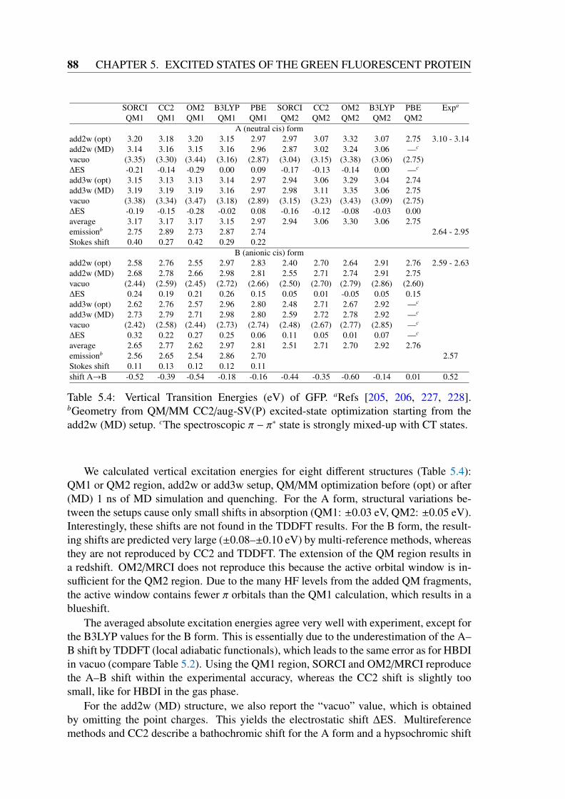
88 CHAPTER 5. EXCITED STATES OF THE GREEN FLUORESCENT PROTEIN
SORCI CC2 OM2 B3LYP PBE SORCI CC2 OM2 B3LYP PBE Expa
QM1 QM1 QM1 QM1 QM1 QM2 QM2 QM2 QM2 QM2A (neutral cis) form
add2w (opt) 3.20 3.18 3.20 3.15 2.97 2.97 3.07 3.32 3.07 2.75 3.10 - 3.14add2w (MD) 3.14 3.16 3.15 3.16 2.96 2.87 3.02 3.24 3.06 —c
vacuo (3.35) (3.30) (3.44) (3.16) (2.87) (3.04) (3.15) (3.38) (3.06) (2.75)∆ES -0.21 -0.14 -0.29 0.00 0.09 -0.17 -0.13 -0.14 0.00 —c
add3w (opt) 3.15 3.13 3.13 3.14 2.97 2.94 3.06 3.29 3.04 2.74add3w (MD) 3.19 3.19 3.19 3.16 2.97 2.98 3.11 3.35 3.06 2.75vacuo (3.38) (3.34) (3.47) (3.18) (2.89) (3.15) (3.23) (3.43) (3.09) (2.75)∆ES -0.19 -0.15 -0.28 -0.02 0.08 -0.16 -0.12 -0.08 -0.03 0.00average 3.17 3.17 3.17 3.15 2.97 2.94 3.06 3.30 3.06 2.75emissionb 2.75 2.89 2.73 2.87 2.74 2.64 - 2.95Stokes shift 0.40 0.27 0.42 0.29 0.22
B (anionic cis) formadd2w (opt) 2.58 2.76 2.55 2.97 2.83 2.40 2.70 2.64 2.91 2.76 2.59 - 2.63add2w (MD) 2.68 2.78 2.66 2.98 2.81 2.55 2.71 2.74 2.91 2.75vacuo (2.44) (2.59) (2.45) (2.72) (2.66) (2.50) (2.70) (2.79) (2.86) (2.60)∆ES 0.24 0.19 0.21 0.26 0.15 0.05 0.01 -0.05 0.05 0.15add3w (opt) 2.62 2.76 2.57 2.96 2.80 2.48 2.71 2.67 2.92 —c
add3w (MD) 2.73 2.79 2.71 2.98 2.80 2.59 2.72 2.78 2.92 —c
vacuo (2.42) (2.58) (2.44) (2.73) (2.74) (2.48) (2.67) (2.77) (2.85) —c
∆ES 0.32 0.22 0.27 0.25 0.06 0.11 0.05 0.01 0.07 —c
average 2.65 2.77 2.62 2.97 2.81 2.51 2.71 2.70 2.92 2.76emissionb 2.56 2.65 2.54 2.86 2.70 2.57Stokes shift 0.11 0.13 0.12 0.12 0.11shift A→B -0.52 -0.39 -0.54 -0.18 -0.16 -0.44 -0.35 -0.60 -0.14 0.01 0.52
Table 5.4: Vertical Transition Energies (eV) of GFP. aRefs [205, 206, 227, 228].bGeometry from QM/MM CC2/aug-SV(P) excited-state optimization starting from theadd2w (MD) setup. cThe spectroscopic π − π∗ state is strongly mixed-up with CT states.
We calculated vertical excitation energies for eight different structures (Table 5.4):QM1 or QM2 region, add2w or add3w setup, QM/MM optimization before (opt) or after(MD) 1 ns of MD simulation and quenching. For the A form, structural variations be-tween the setups cause only small shifts in absorption (QM1: ±0.03 eV, QM2: ±0.05 eV).Interestingly, these shifts are not found in the TDDFT results. For the B form, the result-ing shifts are predicted very large (±0.08–±0.10 eV) by multi-reference methods, whereasthey are not reproduced by CC2 and TDDFT. The extension of the QM region results ina redshift. OM2/MRCI does not reproduce this because the active orbital window is in-sufficient for the QM2 region. Due to the many HF levels from the added QM fragments,the active window contains fewer π orbitals than the QM1 calculation, which results in ablueshift.
The averaged absolute excitation energies agree very well with experiment, except forthe B3LYP values for the B form. This is essentially due to the underestimation of the A–B shift by TDDFT (local adiabatic functionals), which leads to the same error as for HBDIin vacuo (compare Table 5.2). Using the QM1 region, SORCI and OM2/MRCI reproducethe A–B shift within the experimental accuracy, whereas the CC2 shift is slightly toosmall, like for HBDI in the gas phase.
For the add2w (MD) structure, we also report the “vacuo” value, which is obtainedby omitting the point charges. This yields the electrostatic shift ∆ES. Multireferencemethods and CC2 describe a bathochromic shift for the A form and a hypsochromic shift

5.3. RESULTS AND DISCUSSION 89
TD-PBE TD-B3LYP CC2 SORCI OM2/MRCIneutral HBDI (vacuo) -1.2b 0.4 0.8 3.7 1.8anionic HBDI (vacuo) 2.7 1.7 1.6 2.3 1.5GFP A (neutral)a -2.3b 1.0 5.0 5.4 5.8GFP B (anionic)a -0.6b 0.5 3.8 4.6 5.1
Table 5.5: Difference Dipole Moments |µ(S1) − µ(S2)| for the lowest π − π∗ Excitation(debye). aadd2w (MD) GFP setup with QM1 region. bThe minus sign indicates transferof electron density from the imidazole to the phenolate moiety.
for the B form. The latter is partially preserved when omitting the point charges in theQM2 calculation and hence partially caused by residues therein. Interestingly, the ∆ESshift is strongly underestimated by TDDFT methods, TD-PBE even inverts the shift forthe A form.
An explanation for this behavior can be found by analyzing the difference dipole mo-ments, i.e. the charge transfer associated with the excitation (Table 5.5). In vacuo, theS1 ←S0 excitation carries very little charge transfer. SORCI, OM2/MRCI, and CC2predict an increased CT character for this excitation in the protein, in agreement withCASSCF calculations with polarizable continuum models [207]. The obtained differencedipole moment for the B state agrees fairly well with the experimental estimate fromStark spectroscopy at 77 K of 6 debye [206]. Compared with the retinal chromophorein rhodopsins, this CT is still small and explains the moderate influence of the proteinelectrostatic environment. The PBE functional, like other GGA’s strongly underestimatesthe CT and even predicts an inverted direction from the imidazole to the phenolate moietyin most cases. In cases where the π − π∗ state mixes with CT states (not shown), GGA’spredict large unphysical difference dipole moments that are not along the molecular axis.
In Table 5.4, we report also emission energies. The geometries of the fluorescentstate were obtained from excited-state optimization at the CC2 level using a fixed MMenvironment. Based on this structure, all applied methods predict a rather small Stokesshift (0.1 eV) for the B form, in agreement with measurements at 77 K (0.06 eV) and RT(0.14 eV) [229]. A previous CASPT2 study on CASSCF/CHARMM QM/MM geometriesobtained a larger value of 0.29 eV. For the A form, a much larger Stokes shift of 0.3–0.4 eVis predicted. This is within the range of experimental estimates (2.64–2.95 eV) [205, 206],but a reliable experimental reference is missing due to the short lifetime of the A∗ species.A previo us SAC-CI study obtained a slightly larger value of 0.53 eV [230].
5.3.3 QM/MM on a Real-Space Grid
In this section, we test the octopus real space code for QM/MM applications. Instead ofthe basis set, the numerical accuracy of real space calculations is limited by the size of thesimulation box and the grid spacing. The simulation box is defined as a superposition ofatom-centered spheres with a radius R. Octopus offers two ways to calculate an TDDFTabsorption spectrum. For the most common Casida formalism of linear density functionalresponse theory, the number of virtual states nvirt is not limited by the number of basisfunctions and has to be specified as input parameter. Alternatively, the spectrum can be

90 CHAPTER 5. EXCITED STATES OF THE GREEN FLUORESCENT PROTEIN
0.0
0.1
0.2
0.3
0.4
0.5
0.6
2.0 2.5 3.0 3.5 4.0 4.5 5.0 5.5 6.0
exci
tatio
n en
ergy
err
or [e
V]
box radius [Å]
linear responsetime propagation
Figure 5.3: Convergence of the π−π∗ excitation energy in CNH+4 w.r.t. the simulation box
radius. The error refers to an LCAO basis set limit calculation. The SVWN functionalwas used.
obtained from a time propagation of the density. The ground-state density is perturbedby a potential of the form xiδ(t − t0), where xi defines the polarization direction of thelight. The absorption cross section is obtained from the Fourier transformation of thetime-dependent dipole moment. Figure 5.3 illustrates the effect of the two parameters Rand nvirt for a protonated Schiff base (CNH+
4 ) in presence of a point charge (-1.2 e) located2.5 Å from the nitrogen. The Casida-type calculation does not converge to the LinearCombination of Atomic Orbitals (LCAO) limit because a constant nvirt is used. Withincreasing box size, the shape and order of the virtual states changes and convergencewith nvirt can change to the worse. As excited states have in general a more extendeddensity than the ground state, the finite-box error always produces a blue shift, whichsystematically reduces with the parameter R.
When point charges are introduced in a real space QM/MM calculation, the problemarises that electrons can leave the QM region and be bound in regions of low electrostaticpotential. In LCAO, this is prevented by the exponential decay of the atom-centeredbasis functions. In order to investigate this problem in a realistic QM/MM situation,we compare LCAO with octopus results for GFP in the A and B forms using differentQM regions and box sizes. As Figure 5.4 shows, the problem does not occur for theS1 excitation when increasing the box radius to 6 Å and the peak positions converge asexpected. An acceptable error is obtained for values between 2.4 and 3.0 Å, the latter isused in the proceeding calculations.
Figure B.1 shows the time-propagation spectra of TD-PBE using either the QM1 orQM2 region and the effect of the electrostatic embedding. In general, the LCAO results(Table 5.4) are well reproduced. Like in the LCAO case, many CT states occur in theregion of the π − π∗ states and below. Where no mixing occurs, the peak positions agree,reproducing the small blue shift due to the point charges and the underestimated A–Bshift. In many cases, the π − π∗ state couples to CT states, which strongly perturbs the

5.4. CONCLUSIONS 91
0.0
0.5
1.0
1.5
2.0
2.5
3.0
2.7 2.8 2.9 3.0 3.1 3.2
Abs
orpt
ion
(a.u
.)
Energy (eV)
A - R=0.30 nmA - R=0.60 nmB - R=0.24 nmB - R=0.60 nm
Figure 5.4: Effect of the box radius R on the π−π∗ peak position of GFP in A and B form.
spectrum due to redistribution of oscillator strength. For the QM2 calculation of the Bform without point charges, e.g., the absorption band appears splitted. The coupling ofπ − π∗ and CT states occurs in an unpredictable fashion and can drastically change due tosmall structural fluctuations or use of different GGA functionals. In the appendix B, weprovide the spectra from BLYP and LDA functionals, which show the same trends.
5.4 ConclusionsFor both gas phase and GFP environment, our SORCI, OM2/MRCI and CC2 calculationsagree closely with experiment for anionic and neutral protonation states. Our results forthe anionic HBDI in vacuo corroborate the gas-phase measurements of Nielsen et al. [202]and we disagree with Filippi et al. that the vertical excitation energy should be in the range2.92–3.04 eV. We rather see the CASPT2 results critical for the large influence of thezeroth-order Hamiltonian (0.45 eV). Also the EOM-CCSD method, which yields 3.04 eVin [210] tends to overestimate excitation energies of conjugated systems [231].
Our results suggest that neutral HBDI in vacuo is blueshifted by 0.3–0.4 eV comparedto the analog “E” investigated by Rajput et al. [211]. The neutral chromophore in GFPon the other hand is more red-shifted than in any solvent [212] and absorbs 0.4–0.5 eVlower in energy than HBDI in vacuo. On the other hand, the anionic form, which showsmuch larger solvent shifts absorbs rather similar in vacuo and in the protein. Nonetheless,the electrostatic influence of the protein matrix is rather limited in both cases, inline withthe SAC-CI study of Hasegawa et al. [230]. Although the protein environment enhancesthe CT character of the π − π∗ excitation in both A and B forms to ca. 6 debye, theelectrostatic influence of the protein is significantly smaller than in rhodopsins. Largerspectral changes are achieved rather by hydrogen bonds, structural changes and geneticor chemical modification of the chromophore.
DFT (PBE) yields ground-state geometries in good agreement with CC2. TDDFT,however, underestimates the shifts between neutral and anionic form, both in vacuo andin GFP. Further, it underestimates the response to the external field of the protein matrix

92 CHAPTER 5. EXCITED STATES OF THE GREEN FLUORESCENT PROTEIN
due to an underestimated CT upon excitation. TD-PBE even inverts the charge transfer insome cases, leading to an increase of charge density on the phenol ring. Furthermore, aplentitude of artificial CT states appears in the TDDFT spectrum of the neutral A form inGFP, which can lead to perturbed unphysical spectra when these CT states mix with thespectroscopically allowed state. Apart from the shortcomings of the density functionals,the octopus real space code is applicable to QM/MM problems and reproduces the resultsof the LCAO calculations.
Appendix B provides data regarding basis set convergence, parameters of the GBLA, and additionalTDDFT spectra.

5.4. CONCLUSIONS 93
0
1
2
3
4
5
1.5 2 2.5 3 3.5 4
Abs
orpt
ion
(a.u
.)
Energy (eV)
Neutral A, gga pbe, t=60
CT-------------------------------(n+π)→π*-----[ CT ]+[ π → π* ] -------------------
π → π*[ π → π* ] + [ CT ]
π → π*π → π*36 atom, w/o p. ch.
36 atom with p. ch.73 atom, w/o p. ch.73 atom, with p. ch.
0
1
2
3
4
5
1.5 2 2.5 3 3.5 4
Abs
orpt
ion
(a.u
.)
Energy (eV)
Anionic B, gga pbe, t=30
π → n+π*
[ π → π* ] + [ CT ]---- [ CT ] + [ π → π* ]
π → π*π → π*
π → π*
35 atom, w/o p. ch.35 atom with p. ch.73 atom, w/o p. ch.73 atom, with p. ch.
Figure 5.5: Assigned peaks in the time-propagation TD-PBE spectrum of A (upper) andB (lower). Calculations with and without point charges are shown using the QM1 (35atom) and QM2 (73 atom) regions.


Chapter 6
An Exact Expression to Calculate theDerivatives of Position-DependentObservables in Molecular Simulationswith Flexible Constraints
This chapter is based on the article:Pablo Echenique, Claudio N. Cavasotto, Monica De Marco, Pablo Garcia-Risueno andJ. L. Alonso An Exact Expression to Calculate the Derivatives of Position-Dependent Observ-ables in Molecular Simulations with Flexible Constraints, PloS One 6(9): (2011) e24563.
6.1 IntroductionIn the theoretical and computational modeling of physical systems, including but not lim-ited to condensed matter materials [232], fluids [107], and biological molecules [233], itis very common to appeal to the concept of constraints. When a given quantity related tothe system under study is constrained, it is not allowed to depend explicitly on time (oron any other parameter that describes the evolution of the system in the problem at hand).Instead, a constrained quantity is either set to a constant value (hard or rigid constraints)or to a function of the rest of degrees of freedom (flexible, elastic or soft constraints); insuch a way that, if it depends on time, it does so through the latter and not in an explicitmanner.
The imposition of constraints is useful in a wide variety of contexts in the fields ofcomputational Physics and Chemistry: For example, we can use constraints to maintainan exact symmetry of the equations of motion; like in Car-Parrinello Molecular Dynam-ics (MD) [118], where the time-dependent Kohn-Sham orbitals need to be orthonormalalong the time evolution of the quantum-classical system, a requirement that can be ful-filled by imposing constraints over their scalar product [234]. In a different context, wecan use constraints, as in the Blue Moon Ensemble technique [235], to fix some macro-scopic, representative degrees of freedom of molecular systems (normally called reactioncoordinates), in order to be able to compute free energy profiles along them that would
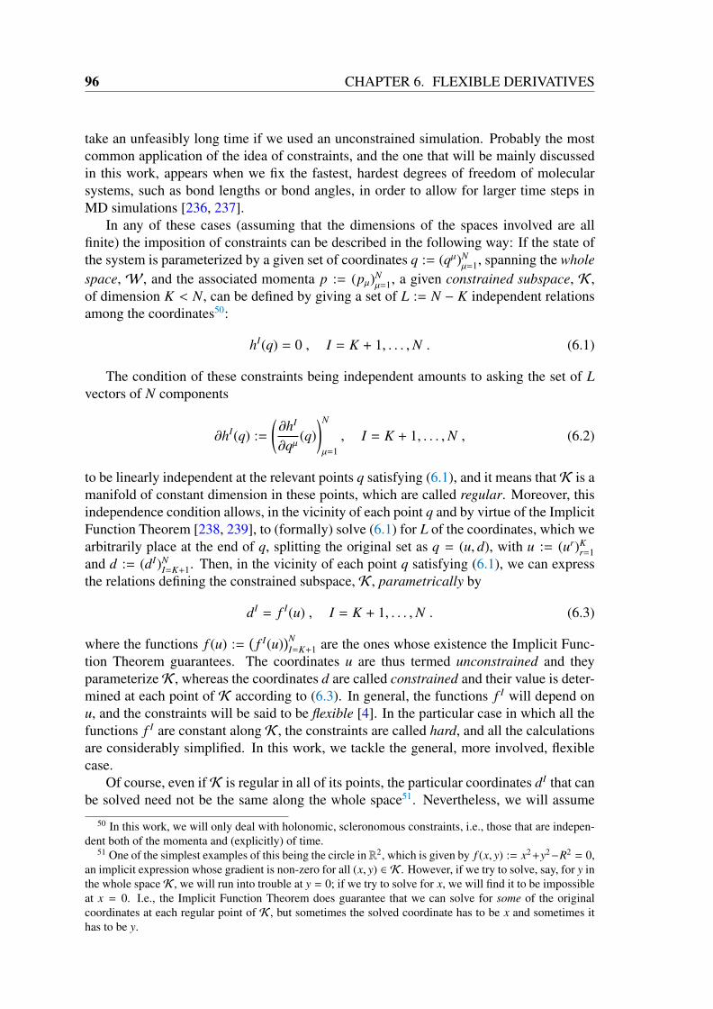
96 CHAPTER 6. FLEXIBLE DERIVATIVES
take an unfeasibly long time if we used an unconstrained simulation. Probably the mostcommon application of the idea of constraints, and the one that will be mainly discussedin this work, appears when we fix the fastest, hardest degrees of freedom of molecularsystems, such as bond lengths or bond angles, in order to allow for larger time steps inMD simulations [236, 237].
In any of these cases (assuming that the dimensions of the spaces involved are allfinite) the imposition of constraints can be described in the following way: If the state ofthe system is parameterized by a given set of coordinates q := (qµ)N
µ=1, spanning the wholespace, W, and the associated momenta p := (pµ)N
µ=1, a given constrained subspace, K ,of dimension K < N, can be defined by giving a set of L := N − K independent relationsamong the coordinates50:
hI(q) = 0 , I = K + 1, . . . ,N . (6.1)
The condition of these constraints being independent amounts to asking the set of Lvectors of N components
∂hI(q) :=(∂hI
∂qµ(q)
)N
µ=1, I = K + 1, . . . ,N , (6.2)
to be linearly independent at the relevant points q satisfying (6.1), and it means thatK is amanifold of constant dimension in these points, which are called regular. Moreover, thisindependence condition allows, in the vicinity of each point q and by virtue of the ImplicitFunction Theorem [238, 239], to (formally) solve (6.1) for L of the coordinates, which wearbitrarily place at the end of q, splitting the original set as q = (u, d), with u := (ur)K
r=1and d := (dI)N
I=K+1. Then, in the vicinity of each point q satisfying (6.1), we can expressthe relations defining the constrained subspace, K , parametrically by
dI = f I(u) , I = K + 1, . . . ,N . (6.3)
where the functions f (u) :=(f I(u)
)NI=K+1 are the ones whose existence the Implicit Func-
tion Theorem guarantees. The coordinates u are thus termed unconstrained and theyparameterizeK , whereas the coordinates d are called constrained and their value is deter-mined at each point of K according to (6.3). In general, the functions f I will depend onu, and the constraints will be said to be flexible [4]. In the particular case in which all thefunctions f I are constant along K , the constraints are called hard, and all the calculationsare considerably simplified. In this work, we tackle the general, more involved, flexiblecase.
Of course, even ifK is regular in all of its points, the particular coordinates dI that canbe solved need not be the same along the whole space51. Nevertheless, we will assume
50 In this work, we will only deal with holonomic, scleronomous constraints, i.e., those that are indepen-dent both of the momenta and (explicitly) of time.
51 One of the simplest examples of this being the circle in R2, which is given by f (x, y) := x2+y2−R2 = 0,an implicit expression whose gradient is non-zero for all (x, y) ∈ K . However, if we try to solve, say, for y inthe whole spaceK , we will run into trouble at y = 0; if we try to solve for x, we will find it to be impossibleat x = 0. I.e., the Implicit Function Theorem does guarantee that we can solve for some of the originalcoordinates at each regular point of K , but sometimes the solved coordinate has to be x and sometimes ithas to be y.
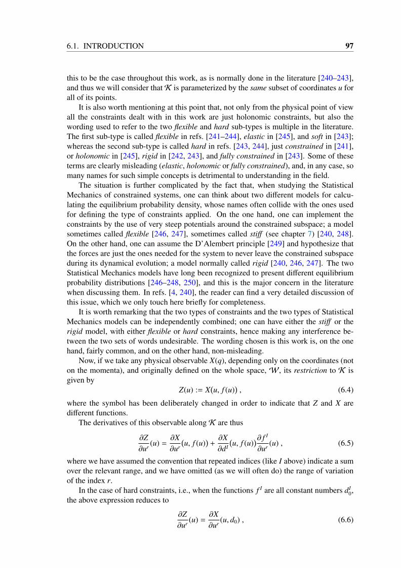
6.1. INTRODUCTION 97
this to be the case throughout this work, as is normally done in the literature [240–243],and thus we will consider thatK is parameterized by the same subset of coordinates u forall of its points.
It is also worth mentioning at this point that, not only from the physical point of viewall the constraints dealt with in this work are just holonomic constraints, but also thewording used to refer to the two flexible and hard sub-types is multiple in the literature.The first sub-type is called flexible in refs. [241–244], elastic in [245], and soft in [243];whereas the second sub-type is called hard in refs. [243, 244], just constrained in [241],or holonomic in [245], rigid in [242, 243], and fully constrained in [243]. Some of theseterms are clearly misleading (elastic, holonomic or fully constrained), and, in any case, somany names for such simple concepts is detrimental to understanding in the field.
The situation is further complicated by the fact that, when studying the StatisticalMechanics of constrained systems, one can think about two different models for calcu-lating the equilibrium probability density, whose names often collide with the ones usedfor defining the type of constraints applied. On the one hand, one can implement theconstraints by the use of very steep potentials around the constrained subspace; a modelsometimes called flexible [246, 247], sometimes called stiff (see chapter 7) [240, 248].On the other hand, one can assume the D’Alembert principle [249] and hypothesize thatthe forces are just the ones needed for the system to never leave the constrained subspaceduring its dynamical evolution; a model normally called rigid [240, 246, 247]. The twoStatistical Mechanics models have long been recognized to present different equilibriumprobability distributions [246–248, 250], and this is the major concern in the literaturewhen discussing them. In refs. [4, 240], the reader can find a very detailed discussion ofthis issue, which we only touch here briefly for completeness.
It is worth remarking that the two types of constraints and the two types of StatisticalMechanics models can be independently combined; one can have either the stiff or therigid model, with either flexible or hard constraints, hence making any interference be-tween the two sets of words undesirable. The wording chosen is this work is, on the onehand, fairly common, and on the other hand, non-misleading.
Now, if we take any physical observable X(q), depending only on the coordinates (noton the momenta), and originally defined on the whole space, W, its restriction to K isgiven by
Z(u) := X(u, f (u)
), (6.4)
where the symbol has been deliberately changed in order to indicate that Z and X aredifferent functions.
The derivatives of this observable along K are thus
∂Z∂ur (u) =
∂X∂ur
(u, f (u)
)+∂X∂dI
(u, f (u)
)∂ f I
∂ur (u) , (6.5)
where we have assumed the convention that repeated indices (like I above) indicate a sumover the relevant range, and we have omitted (as we will often do) the range of variationof the index r.
In the case of hard constraints, i.e., when the functions f I are all constant numbers dI0,
the above expression reduces to
∂Z∂ur (u) =
∂X∂ur (u, d0) , (6.6)

98 CHAPTER 6. FLEXIBLE DERIVATIVES
where X(q) must be a known function of q (in order to have a well-defined problem),and its derivative is typically easy to compute. However, if the constraints are of themore general, flexible form (the ones tackled in this work), the calculation of the partialderivatives (∂ f I/∂ur)(u) cannot be avoided.
If the constraints are assumed to be flexible, it is common in the literature of molecu-lar modeling to define these functions f I(u) as the values taken by the coordinates d if weminimize either the total or the potential energy with respect to all dI at fixed u [4, 240–243]. Since the energy functions used in molecular simulation are typically rather compli-cated, such as the ones in classical Force Fields, with a large number of distinct functionalterms [99, 115, 251–254], or the effective nuclear potential arising from the solution ofthe electronic Schrödinger equation in the ground-state Born-Oppenheimer approxima-tion [50, 240], the minimization of the energy with respect to the coordinates d has to beperformed numerically. Hence, the functions f I(u), which are the output of this process,do not have a compact analytical expression that can be easily differentiated to include itin eq. (6.5).
In this work, we present a parameter-free, exact algorithm (up to machine precision)to calculate the derivatives (∂ f I/∂ur)(u) in such a case. Although several methods existin the literature [241–243] for performing MD simulations with flexible constraints, no-body has dealt, as far as we are aware, with the computation of these derivatives. Sincethe general idea can be applied to any situation in which (1) we have flexible constraints,(2) that are defined in terms of the minimization of some quantity with respect to theconstrained coordinates, we first introduce, the essential part of the algorithm based onthese two points. Then, we develop a more sophisticated application of this idea to thecalculation of the derivatives along the constrained subspace of the Euclidean coordinatesof molecular systems; a problem that we faced in our group when trying to calculate thecorrecting terms associated to mass-metric tensor determinants that appear in the equilib-rium probability density when constraints are imposed [4, 240, 255]. Finally, we performa comparison between the results obtained with our exact algorithm and the calculationof the derivatives by finite differences; this serves the double purpose of numerically val-idating the algorithm and showing the limitations of the latter method, which needs thetuning of a parameter for each particular problem.
6.2 Methods
6.2.1 General Algorithm
As we mentioned in the Introduction, we assume that we are dealing with a constrainedproblem in which the functions f I(u) in eq. (6.3) are defined as taking the values of theconstrained coordinates dI that minimize52 a given function, V(q) = V(u, d), for each fixedu, i.e.,
V(u, f (u)
)≤ V(u, d) , ∀d ∈ D
(f (u)
), (6.7)
52 Depending on the particular application, one can ask the minimum that defines the functions f I(u) tobe global or just local. However, in the cases in which V is the total or the potential energy of a complexmolecular system, it may become very difficult to find its global minimum (resulting from the shear numberof dimensions of the search space), and the local choice is the only reasonable one [4].

6.2. METHODS 99
whereD(f (u)
)is a suitable open set in RL containing the point f (u).
In order to calculate the derivatives along K of any physical observable function ofthe coordinates Z(u) := X
(u, f (u)
), like the one defined in (6.4), we can always follow the
finite-differences approach. However, as we discuss in the Results and Discussion section,finite differences presents intrinsic inaccuracies which are difficult to overcome, speciallyas the system grows larger. Let us now introduce a different way to calculate (∂Z/∂ur)(u)which does not suffer from this drawback.
The starting point is eq. (6.5) in the Introduction, which we copy here for the comfortof the reader:
∂Z∂ur (u) =
∂X∂ur
(u, f (u)
)+∂X∂dI
(u, f (u)
)∂ f I
∂ur (u) . (6.8)
As we mentioned, the expression of X(q), as well as the functions f I(u), must beknown if we wish to have a well-defined constrained problem to begin with. Therefore,the only objects that remain to be computed are the partial derivatives (∂ f I/∂ur)(u).
If we assume that we have available some method to check that the order of the sta-tionary point is the appropriate one (i.e., that it is a minimum, and not a maximum or asaddle point), we can write a set of equations which are equivalent to eq. (6.7), and which(implicitly) define the functions f I(u):
∂V∂dI
(u, f (u)
)= 0 , I = K + 1, . . . ,N . (6.9)
Now, we can take the derivative of this expression with respect to a given uncon-strained coordinate ur:
∂2V∂ur∂dI
(u, f (u)
)︸ ︷︷ ︸HrI(u)
+∂2V∂dJ∂dI
(u, f (u)
)︸ ︷︷ ︸HJI(u)
∂ f J
∂ur (u)︸ ︷︷ ︸F J
r (u)
= 0 , (6.10)
where Hµν(u), with µ, ν = 1, . . . ,N, is the Hessian matrix of V evaluated at(u, f (u)
)∈ K ,
and F Jr (u) is the matrix of unknowns that we want to solve for53. It is worth mentioning
that similar equations to the ones above can be found in classical mechanics anytime thatlocal coordinates are used (the coordinates u in this work). For example, the force insuch a case is defined as ∂V/∂ur and the chain rule can be used in a similar way to whatwe do here. Note, however, that eq. (6.9) does not contain derivatives with respect tour, but to the constrained coordinate dI . This makes the approach slightly different and,indeed, eq. (6.10) would become trivial in the most common hard situation tackled in theliterature, where ∂ f J/∂ur = 0, ∀J, r.
Since we are, by hypothesis, in a minimum of V with respect to the constrained coor-dinates d, the constrained sub-block HJI(u) of the Hessian is a positive definite matrix, andtherefore invertible. Hence, if we multiply eq. (6.10) by its inverse, denoted by HIM(u),sum over I, exploit the fact that Hµν(u) and Hµν(u) are symmetric, and conveniently re-name the indices, we arrive at:
∂ f I
∂ur (u) =: F Ir(u) = −HIJ(u)HJr(u) , (6.11)
53 In the whole document, we adhere to the practice of using different types of indices in order to indicatedifferent ranges of variation. Here, for example, µ, ν, ρ, . . . run from 1 to N; r, s, t, . . . run from 1 to K; andI, J,M, . . . run from K + 1 to N. In the next section, we need to use more types of indices, but the idea is thesame.

100 CHAPTER 6. FLEXIBLE DERIVATIVES
which, as promised, allows us to find the exact derivatives (∂ f I/∂ur)(u) with the onlyknowledge of the Hessian of V at the point
(u, f (u)
), and, upon introduction of the result in
eq. (6.8), also the derivatives along the constrained subspaceK of any physical observableX(q).
As mentioned, several methods exist in the literature [241–243] to perform MD sim-ulations with flexible constraints, however, none of them has tackled the calculation ofthese derivatives, which are very basic objects presumably to be needed in many futureapplications (see, e.g., refs. [4, 240]). Of course, it is always possible to compute deriva-tives using the simple and straightforward method of finite differences. In this work, weuse finite differences as a way of validating the new, exact method and ensuring it is errorfree.
The accuracy of the new algorithm is only limited by the accuracy with which we cancalculate the Hessian of V at
(u, f (u)
)and invert it; there is no tunable parameter that we
need to adjust for optimal accuracy, as in the case of finite differences (see below and alsoResults and Discussion). This makes a difference because, in classical Force Fields [99]and even in some quantum chemical methods (e.g., see chap. 10 of [51]), the Hessian canbe calculated analytically, without the need of finite differences.
Although no optimization of the numerical cost has been pursued in this work, someremarks can be made about it, in comparison with the cost of the finite-differences ap-proach. In order to calculate the partial derivatives ∂Z/∂us with respect to the uncon-strained coordinates u using finite differences, we need to:
é Minimize V(u, d) at fixed u to find f (u).
é Calculate Z(u) := X(u, f (u)
).
é Choose a displacement ∆ and minimize V(u, d) at the point u := (ur)Kr=1, where
ur = ur +∆ if r = s and ur = ur if r , s. This yields f (u) at a nearby point inK withus displaced a quantity ∆ and the rest of unconstrained coordinates kept the same.
é Calculate Z(u) := X(u, f (u)
).
é Calculate∆Z∆us :=
Z(u) − Z(u)∆
(6.12)
as the finite-difference approximation to the sought derivative ∂Z/∂us at the point u.
Note that the third point of this finite-differences approach is essentially a linear sta-bility analysis. When strongly non-equilibrium points are present, such as in the examplesdiscussed in the last section, this approximation fails and the fact that the new algorithmintroduced in this work uses only quantities defined at the point u becomes even moreimportant.
Now, assuming that we have a good enough guess for the parameter ∆, the cost of thisprocedure is dominated by the need to perform K minimizations of the function V , onein each of the directions corresponding to the unconstrained coordinates ur. If we denoteby Nit the average number of iterations needed for these minimizations to converge, andwe define CV and CdV as the numerical costs (in computer time) of computing V andits first derivatives with respect to the constrained coordinates d, respectively, we have

6.2. METHODS 101
that the average cost of calculating the sought derivatives ∂Z/∂ur using finite differenceswill be KNit(CV + CdV) for local optimization methods such as the steepest descent or theconjugate gradient, or KN′itCV for Monte Carlo-based methods in which the derivatives ofV are not needed, such as simulated annealing [256].
On the other hand, the new algorithm does not require the extra minimizations, but itdoes require the calculation of the Hessian of V with respect to the internal coordinates(whose cost we call CH), and the computation of the inverse of its constrained sub-block,HJI , applied to each one of the K L-vectors Fr in eqs. (6.10) and (6.11), of cost CiH;resulting in a total cost of CH + KCiH.
The comparison between the two costs is not trivial and some remarks about it must bemade: First, one must notice that the different individual costs involved, CV , CdV , CH andCiH, are strongly dependent on the characteristics (1) of the coordinates q used and (2) ofthe function V(q). For example, if the coordinates q are the Euclidean ones and the func-tion V(q) is the potential energy of a molecular system as modeled by a typical Force Field[99, 115, 251–254], the most direct algorithms for calculating V and its derivatives yieldcosts CV , CdV and CH which are of order N2, NK and N2, respectively [233]. However,if more advanced long-range techniques are used, such as the particle-particle particle-mesh (P3M) method [257], the fast multipole method [258] or the particle-mesh Ewaldsummation [96], these costs can be reduced to order N log N or even N (for large N andforgetting prefactors). Also, as mentioned, if the coordinates used are not the Euclideanones but some internal coordinates such as the ones used in this work, these costs mustchange in order to account for the transformation between the two. If force fields are notused but, instead, V(q) is the ground-state Born-Oppenheimer energy as calculated usingHartree-Fock [50], then the most naive implementations yield costs for CV , CdV and CH
which are of order N4 [51]. The cost, CiH, of calculating the inverse of HJI applied toa vector Fr can range from order N to order N3 depending on the sparsity of the matrix[256], which, in turn, depends again on the coordinates used and on the structure of V(q).Finally, additional qualifications may complicate the comparison, such as the architectureof the computers in which the algorithms are implemented, parallelization issues, or thefact that, e.g., if we need the Hessian for a different purpose in our simulation, such asthe calculation of the corresponding correcting term that appears both in the constrainedstiff model and in the Fixman potential [240], then the “only” computational step we areadding is the inversion of a matrix.
Despite the complexity and problem-dependence of the cost assessment, it must bestressed that, even in the cases in which the new algorithm turns out to be more expensivethan the alternatives, the fact that it is exact and parameter-free might still make it thepreferred choice in problems where high accuracy is needed. Although a parameter-freestructure does not guarantee higher accuracy, in this case it does, since our method canbe identified as the proper limit of the finite-differences scheme when ∆ → 0. This isillustrated in Results and Discussion.
It is also worth remarking that the new method, as mentioned, is not needed to performMD simulations, which can be run without calculating any of the derivatives tackled inthis work [241–243]. Our method is only needed when some observable in which thesederivatives are included (such as the aforementioned mass-metric tensor determinants)needs to be computed. In such cases, the only two options to get to the final result areeither finite differences or our method, and the most convenient of the two has to be

102 CHAPTER 6. FLEXIBLE DERIVATIVES
chosen; even if its cost is a burden.
6.2.2 Application to Euclidean coordinates of MoleculesIn this section, we will apply the general algorithm introduced above to calculate thederivatives along the constrained subspace of the Euclidean coordinates of molecular sys-tems in a Frame of Reference (FoR) fixed in the molecule. This problem has been faced byour group when trying to calculate the correcting terms associated with mass-metric tensordeterminants that appear in the equilibrium probability density when flexible constraintsare imposed [4, 240, 255]. More specifically, these derivatives are needed to calculatethe determinant of the induced mass-metric tensor g that appears in the constrained rigidmodel, according to the formulae derived in ref. [255].
In such a case, the system of interest is a set of n mass points termed atoms. Thethree Euclidean coordinates of atom α in a FoR fixed in the laboratory are denoted by ~xα,and its mass by mα, with α = 1, . . . , n. However, when no explicit mention to the atomindex needs to be made, we will use x := (xµ)N
µ=1 to denote the N-tuple of all the N := 3nEuclidean coordinates of the system. The masses N-tuple, m := (mµ)N
µ=1, in such a case,is formed by consecutive groups of three identical masses, corresponding to each of theatoms.
Apart from the Euclidean coordinates, one can also use a given set of curvilinearcoordinates (also called sometimes general or generalized), denoted by q := (qµ)N
µ=1, todescribe the system. Both the coordinates x and q parameterize the whole spaceW, andthe transformation between the two sets and its inverse are respectively given by
xµ = Xµ(q) , µ = 1, . . . ,N , (6.13a)qµ = Qµ(x) , µ = 1, . . . ,N . (6.13b)
We will additionally assume that, for the points of interest, this is a proper change ofcoordinates, i.e., that the Jacobian matrix
Jµν :=∂Xµ(q)∂qν
(6.14)
has non-zero determinant.Now, we define a particular FoR fixed in the system to perform some of the calcula-
tions. To this end, we select three atoms (denoted by 1, 2 and 3) in such a way that ~o,the position in the FoR of the laboratory of the origin of the FoR fixed in the system, isthe Euclidean position of atom 1 (i.e., ~o := ~x1). The orientation of the FoR (x ′, y ′, z ′)fixed in the system is chosen such that atom 2 lies in the positive half of the z ′-axis, andatom 3 is contained in the (x ′, z ′)-plane, with projection on the positive half of the x ′-axis(see fig. 6.1). The position of any given atom α in the new FoR fixed in the system isdenoted by ~x ′α. Also, let E(φ, θ, ψ) be the Euler rotation matrix (in the ZYZ convention)that takes a free 3-vector of primed components, ~a ′, to the FoR fixed in the laboratory,i.e., ~a = E(φ, θ, ψ)~a ′ [249].
Although the aforementioned curvilinear coordinates q are a priori general, it is verycommon to take into account the fact that the typical potential energy functions of molec-ular systems in absence of external fields do not depend on ~oT := (ox, oy, oz) nor on the

6.2. METHODS 103
Figure 6.1: Definition of the frame of reference fixed in the system.
angles (φ, θ, ψ), and to consequently choose a set of curvilinear coordinates split into q =
(e, r), where the first six are these external coordinates, e := (eA)6A=1 = (ox, oy, oz, φ, θ, ψ).
As we mentioned before, ~o := (ox, oy, oz) describes the overall position of the system withrespect to the FoR fixed in the laboratory, and its overall orientation is specified by the an-gles (φ, θ, ψ). The remaining N −6 coordinates r := (ra)N
a=7 are called internal coordinatesand determine the positions of the atoms in the FoR fixed in the system [92, 259]. Theyparameterize what we shall call the internal subspace or conformational space, denotedby I, and the coordinates e parameterize the external subspace, denoted by E; conse-quently splitting the whole space asW = E × I (denoting by × the Cartesian product ofsets).
The position, ~x ′α, of any given atom α in the axes fixed in the system is a function,~X ′α(r), of only the internal coordinates, r, and the transformation from the Euclidean co-ordinates x to the curvilinear coordinates q in (6.13a) may be written more explicitly asfollows:
~xα = ~Xα(q) = ~o + E(φ, θ, ψ) ~X ′α(r) . (6.15)
Although general constraints affecting all the coordinates q [like those in (6.1)] canbe imposed on the system, the already mentioned property of invariance of the potentialenergy function under changes of the external coordinates, e, together with the fact thatthe potential energy can be regarded as “producing” the constraints [240], make physicallyfrequent the use of constraints involving only the internal coordinates, r:
hI(r) = 0 , I = K + 1, . . . ,N . (6.16)
Under the common assumptions in the Introduction, these constraints allow us to splitthe internal coordinates as r = (s, d), where the first M := K − 6 = N − L − 6 ones,s := (si)K
i=6+1, are called unconstrained internal coordinates and parameterize the internalconstrained subspace, denoted by Σ. The last L := N−K ones, d := (dI)N
I=K+1, correspondto the constrained coordinates in the Introduction and are called. The external coordi-nates, e, together with the unconstrained internal coordinates, s, constitute the set of all

104 CHAPTER 6. FLEXIBLE DERIVATIVES
unconstrained coordinates of the system, u = (e, s), which parameterize the constrainedsubspace K , being K = E × Σ.
In this situation, the constraints in eq. (6.16) are equivalent to
dI = f I(s) , I = K + 1, . . . ,N , (6.17)
and the functions f I(s) are defined as taking the values of the coordinates dI that minimizethe potential energy with respect to all dI at fixed s [4, 240, 243].
Finally, if these constraints are used, together with (6.15), the Euclidean position ofany atom in the constrained case may be parameterized with the set of all unconstrainedcoordinates, u, as follows:
~xα = ~Zα(u) := ~Xα
(e, s, f (s)
)= ~o + E(φ, θ, ψ)~X ′α
(s, f (s)
)=: ~o + E(φ, θ, ψ)~Z ′α(s) , (6.18)
where the name of the transformation functions has been changed from X to Z, and fromX ′ to Z ′, in order to emphasize that the dependence on the coordinates is different betweenthe two cases.
In order to calculate the derivatives along Σ of the primed atoms positions, ~Z ′α, withrespect to the unconstrained internal coordinates s (needed, for example, in eq. (28) ofref. [255] to compute the determinant of the induced mass-metric tensor g), we first dif-ferentiate with respect to si in ~Z ′α(s) := ~X ′α
(s, f (s)
), arriving to the analogue to eq. (6.8):
∂~Z ′α∂si (s) =
∂~X ′α∂si
(s, f (s)
)+∂~X ′α∂dI
(s, f (s)
)∂ f I
∂si (s) . (6.19)
Now, the derivatives (∂ f I/∂si)(s) can be calculated using the general algorithm intro-duced in the previous section simply noticing that, in this case, V is precisely the potentialenergy of the system. Therefore, the only objects that remain to be computed are thederivatives ∂~X ′α/∂si and ∂~X ′α/∂dI , which can be known analytically (they are geometri-cal [or kinematical] objects, i.e., they do not depend of the potential energy). We nowturn to the derivation of an explicit algorithm for finding them and thus completing thecalculation that is the objective of this section.
In the supplementary material of ref. [255], we give a detailed and explicit way forexpressing any “primed” vector ~X ′α as a function of all the internal coordinates, in the par-ticular coordination scheme known as SASMIC [92]. We could take the final expressionthere [eq. (5)] and explicitly perform the partial derivatives, however, we shall follow adifferent approach that is both more straightforward and applicable to a larger family ofZ-matrix-like schemes for defining internal coordinates.
In non-redundant internal coordinates schemes, whether they are defined as in ref. [92]or not, each atom is commonly regarded as being incrementally added to the growingmolecule for its coordination. This means that the position of the (α > 3)-th atom in thebody-fixed axes is uniquely specified by the values of three internal coordinates that aredefined with respect to the positions of three other atoms with indices β(α), δ(α), γ(α) < α.This is a very convenient practice, and we will assume that we are dealing with a schemethat adheres to it.
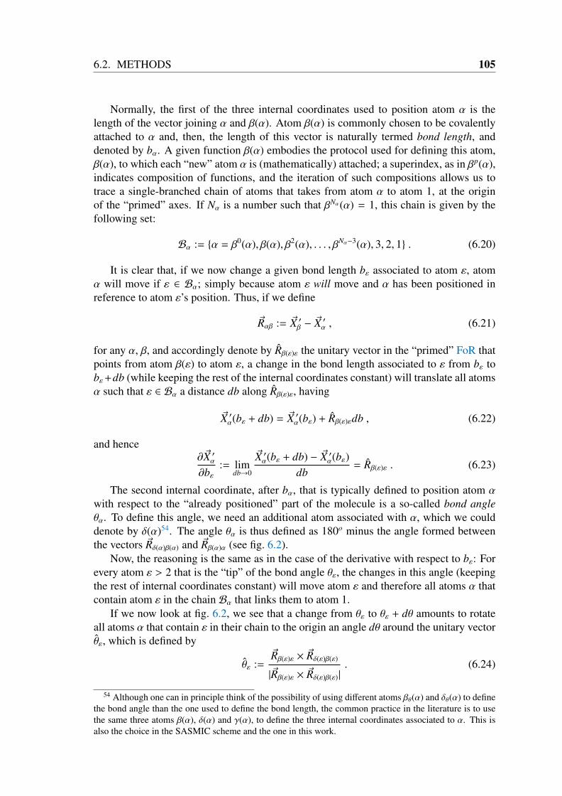
6.2. METHODS 105
Normally, the first of the three internal coordinates used to position atom α is thelength of the vector joining α and β(α). Atom β(α) is commonly chosen to be covalentlyattached to α and, then, the length of this vector is naturally termed bond length, anddenoted by bα. A given function β(α) embodies the protocol used for defining this atom,β(α), to which each “new” atom α is (mathematically) attached; a superindex, as in βp(α),indicates composition of functions, and the iteration of such compositions allows us totrace a single-branched chain of atoms that takes from atom α to atom 1, at the originof the “primed” axes. If Nα is a number such that βNα(α) = 1, this chain is given by thefollowing set:
Bα := α = β0(α), β(α), β2(α), . . . , βNα−3(α), 3, 2, 1 . (6.20)
It is clear that, if we now change a given bond length bε associated to atom ε, atomα will move if ε ∈ Bα; simply because atom ε will move and α has been positioned inreference to atom ε’s position. Thus, if we define
~Rαβ := ~X ′β − ~X′α , (6.21)
for any α, β, and accordingly denote by Rβ(ε)ε the unitary vector in the “primed” FoR thatpoints from atom β(ε) to atom ε, a change in the bond length associated to ε from bε tobε+db (while keeping the rest of the internal coordinates constant) will translate all atomsα such that ε ∈ Bα a distance db along Rβ(ε)ε, having
~X ′α(bε + db) = ~X ′α(bε) + Rβ(ε)εdb , (6.22)
and hence∂~X ′α∂bε
:= limdb→0
~X ′α(bε + db) − ~X ′α(bε)db
= Rβ(ε)ε . (6.23)
The second internal coordinate, after bα, that is typically defined to position atom αwith respect to the “already positioned” part of the molecule is a so-called bond angleθα. To define this angle, we need an additional atom associated with α, which we coulddenote by δ(α)54. The angle θα is thus defined as 180o minus the angle formed betweenthe vectors ~Rδ(α)β(α) and ~Rβ(α)α (see fig. 6.2).
Now, the reasoning is the same as in the case of the derivative with respect to bε: Forevery atom ε > 2 that is the “tip” of the bond angle θε, the changes in this angle (keepingthe rest of internal coordinates constant) will move atom ε and therefore all atoms α thatcontain atom ε in the chain Bα that links them to atom 1.
If we now look at fig. 6.2, we see that a change from θε to θε + dθ amounts to rotateall atoms α that contain ε in their chain to the origin an angle dθ around the unitary vectorθε, which is defined by
θε :=~Rβ(ε)ε × ~Rδ(ε)β(ε)
|~Rβ(ε)ε × ~Rδ(ε)β(ε)|. (6.24)
54 Although one can in principle think of the possibility of using different atoms βθ(α) and δθ(α) to definethe bond angle than the one used to define the bond length, the common practice in the literature is to usethe same three atoms β(α), δ(α) and γ(α), to define the three internal coordinates associated to α. This isalso the choice in the SASMIC scheme and the one in this work.

106 CHAPTER 6. FLEXIBLE DERIVATIVES
Figure 6.2: Rotation associated to a change in a bond angle. Definition of the bondangle θε, associated to atom ε, and the unitary vector θε corresponding to the directionaround which all atoms α with chains Bα containing ε rotate if θε is varied while the restof internal coordinates are kept constant.
The result, ~vrot, of rotating a vector ~v around the direction given by the unitary vectorθ an amount θ is given by the well-known Rodrigues’ rotation formula [249, 260]:
~vrot = ~v cos θ + (θ × ~v) sin θ + θ(θ · ~v)(1 − cos θ) . (6.25)
However, notice that, in order to define a rotation, it is not enough to specify the angleθ and the rotation axis θ, but one additionally needs to specify a fixed point (which canactually be any of the points in a fixed line in the direction of θ). Therefore, the aboveexpression is only correct for either “free” vectors ~v (i.e., those that are not associated toa given point in space), or for vectors ~v whose starting point lies in the aforementionedfixed line.
The fixed point for the rotation we are interested in can be chosen to be β(ε) and, usingeq. (6.25), we have that
~Rβ(ε)α(θε + dθ) = ~Rβ(ε)α(θε) cos dθ
+[θε × ~Rβ(ε)α(θε)
]sin dθ (6.26)
+ θε[θε · ~Rβ(ε)α(θε)
](1 − cos dθ) .
Then, keeping the terms up to first order in dθ, we can easily compute the derivative:
∂~Rβ(ε)α
∂θε= θε × ~Rβ(ε)α , (6.27)
which, since a variation of θε does not move atom β(ε) (i.e. ∂~X ′β(ε)/∂θε = 0), allows us toconclude that
∂~X ′α∂θε
=∂
∂θε
(~X ′β(ε) + ~Rβ(ε)α
)=∂~Rβ(ε)α
∂θε= θε × ~Rβ(ε)α , (6.28)
if ε ∈ Bα.The third and last internal coordinate that is usually defined to position atom α is a
so-called dihedral angle ϕα. To define this angle, we need a third atom associated with α,which we could denote by γ(α). The angle ϕα is thus defined as the oriented angle formed

6.2. METHODS 107
between the plane containing atoms β(α), δ(α) and γ(α) and the plane containing atoms α,β(α) and δ(α). The positive direction of ϕα is the one indicated in fig. 6.3, and, although itis common to find two different covalent arrangements of the four atoms α, β(α), δ(α) andγ(α), termed principal and phase dihedral angles, respectively [92], this does not affectthe mathematical definition of ϕα given in this paragraph, nor the subsequent calculations.
Figure 6.3: Rotation associated to a change in a dihedral angle. Definition of thedihedral angle ϕε, associated to atom ε. The positive direction of rotation is indicated inthe figure, and we can distinguish between two situations regarding covalent connectivity:a) principal dihedral angle, and b) phase dihedral angle (see ref. [92]).
Regarding the derivative of the “primed” position of atom α with respect to a givenϕε, the only difference with the bond angle case is that, now, the rotation is performedaround the direction given by the unitary vector Rδ(ε)β(ε) (see fig. 6.3). The fixed point canbe again chosen as β(ε), and eq. (6.27) (changing θε by ϕε and θε by Rδ(ε)β(ε)), as well asthe fact that changes in ϕε do not move atom β(ε), still hold. Therefore,
∂~X ′α∂ϕε
= Rδ(ε)β(ε) × ~Rβ(ε)α , (6.29)
if ε ∈ Bα.In order to decide whether or not atom α will move upon changes in internal coordi-
nates associated to atoms ε that do not belong to Bα we must first finish the story aboutinternal coordinates definition. Since the argument above to show that α moved whenε ∈ Bα was that ε itself moved and it was used to position α, we must ask

108 CHAPTER 6. FLEXIBLE DERIVATIVES
é whether or not there can be atoms that are also used to position α but that do notbelong to Bα, and
é what happens when we change the internal coordinates associated to them.
The answers to these two questions depend on the particular scheme used to definethe internal coordinates, and we will tackle them referring to the SASMIC scheme [92],which is the one used in this work: According to the SASMIC rules, there are only twosituations in which an atom ε < Bα can be used to position atom α, and they are depictedin fig. 6.4.
Figure 6.4: Special cases. Special cases of atoms that do not belong to the chain Bαconnecting α to atom 1, but that are nevertheless used to position α.
The first case, in fig. 6.4a, attains only the first atoms of the molecule. Typically,atom 1 is not a first-row atom, but a Hydrogen (such is the case of the three moleculesstudied, for example, in Results and Discussion). Hence, after positioning atoms 2 and3, which are typically first-row, it is more representative to choose atom 3 as δ(α) andatom 1 as γ(α) when positioning the rest of the atoms α attached to atom 2. This makes1 = β2(α) , δ(α) and hence δ(α) qualifies as an atom that is used to position α but whichis not included in the chain Bα.
The second case, in fig. 6.4b, corresponds to the situation in which the molecule di-vides into two branches, and it can happen all along its chemical structure. If atom ε is theatom that defines the only principal dihedral over the bond connecting δ(ε) and β(ε) (in

6.2. METHODS 109
the SASMIC scheme, only one principal dihedral can be defined on a given bond [92]),and atom α belongs to a different branch than the one beginning in ε (the branches areindicated with grey broad arrows), then the starting atom ε′ of the branch to which α be-longs (ε′ can be α itself) must be positioned using a phase dihedral in which ε = γ(ε′).Thus, ε is an atom that is used to position α, but which does not belong to the chain Bαconnecting α to atom 1.
In principle, any change in the internal coordinates of atom δ(α), in the first case,or in those of atom ε, in the second case, may move atom α, however, because of thegeometrical characteristics of the internal coordinates, this is not the case.
For example, it is easy to see that, in the case depicted in fig. 6.4a, a variation of thebond length bε (denoting ε := δ(α)) does not move atom α. Regarding the angles, thedihedral ϕε is not defined because ε = 3, and a change in θε can be seen to rotate atomα with fixed point β(ε) = β(α) and around the axis given exactly by θε as defined ineq. (6.24)55. Therefore, the derivative of the Euclidean position of atom α with respect toθε is also given by eq. (6.28) in this special case.
In the situation shown in fig. 6.4b, one can see that neither a change in bε nor in θεmove atom ε′ nor α. However, if we change ϕε, we need to move atom ε′ if we want tokeep ϕε′ constant. Therefore, atom α moves in such a case and it does so by rotating withthe same fixed point β(ε) and the same axis Rδ(ε)β(ε) as in the simpler cases depicted infig. 6.3. This means that, again, we can calculate the sought derivative using the alreadyjustified eq. (6.29).
In summary, only changes in bond lengths associated to atoms ε ∈ Bα affect theposition of atom α:
∂~X ′α∂bε
=
Rβ(ε)ε if ε ∈ Bα0 if ε < Bα
; (6.30)
changes both in bond angles associated to atoms ε ∈ Bα and to δ(α) in fig. 6.4a affect theposition of atom α:
∂~X ′α∂θε
=
θε × ~Rβ(ε)α if ε ∈ Bα ,
or[β(α) = 2, δ(α) = 3)
]0 otherwise
; (6.31)
and changes both in dihedral angles associated to atoms ε ∈ Bα and to those that definethe principal dihedral at a branching point that leads to atom α (see fig. 6.4b) can affectthe position of atom α:
∂~X ′α∂ϕε
=
Rδ(ε)β(ε) × ~Rβ(ε)α if ε ∈ Bα ,
or[ϕε ppal., β(ε) ∈ Bα
]0 otherwise
. (6.32)
Finally, the outline of the algorithm for calculating the sought derivatives ∂~X ′α(s, f (s)
)/∂si
along the constrained subspace Σ is:
55 It is not trivial to see that this motion keeps all the rest of internal coordinates constant, specially thephase dihedral ϕα. The authors found it helpful to imagine that atoms 1, 2 and 3 lie in the plane of the paper,with θε and α coming out of it towards the reader; the first orthogonally and the second not.
110 CHAPTER 6. FLEXIBLE DERIVATIVES
é Calculate the chain Bα that connects atom α with atom 1 and identify the specialcases depicted in fig. 6.4.
é Calculate the derivatives ∂ f I/∂si by solving the system of linear equations in (6.11).
é Calculate the geometric derivatives ∂~X ′α(r)/∂si and ∂~X ′α(r)/∂dI , for I = K+1, . . . ,N,using eqs. (6.30), (6.31) and (6.32).
é Plug all the calculated quantities into eq. (6.19) et voilà.
6.3 Results and DiscussionIn this section, we compare the finite-differences approach (see Methods) to the new al-gorithm introduced in this work with two objectives in mind: the validation of the newscheme, and the identification of the most important pitfalls of the finite-differences tech-nique, which are absent in the new method. It is worth stressing again that the methodpresented here is the first of its kind, as far as we are aware, and the finite-differencesscheme is just a very natural and straightforward method that is always available whenderivatives need to be calculated. In fact, the pitfalls of finite differences which we high-light in this section are very well known, although they have been seldomly presented inthe context of molecular Force Fields. We hope that this section can be additionally usefulto revisit this classical topic from a new angle.
To these two ends, we have applied the more specific algorithm introduced in the pre-vious section for the calculation of the derivatives of the Euclidean coordinates of molec-ular systems to the three biological species in fig. 6.5: methanol, N-methyl-acetamide(NMA), and the tripeptide N-acetyl-glycyl-glycyl-glycyl-amide (GLY3). For each one ofthese molecules, a number of dihedral angles describing rotations around single bonds(and indicated with light-blue arrows in fig. 6.5) have been chosen as the unconstrainedinternal coordinates, s, spanning the corresponding constrained internal subspace Σ. Therest of internal coordinates d (bond lengths, bond angles, phase dihedrals, and princi-pal dihedrals over non-single bonds) are flexibly constrained as described in the previoussections. The numeration of the atoms and the definition of the internal coordinates fol-low the SASMIC scheme, which is specially adapted to deal with constrained molecularsystems [92].
For methanol and NMA, as a result of the small dimensionality of their constrainedsubspaces, the working sets of conformations have been generated by systematically scan-ning their unconstrained internal coordinates at finite steps. For methanol, we produced19 conformations, in which the central dihedral, ϕ6, ranges from 0o to 180o in steps of10o. Similarly, the systematic scanning of the unconstrained dihedrals in NMA produceda set of 588 conformations in which the first and last angles, ϕ6 and ϕ10, range from 0o
to 180o, and the central one, ϕ8, ranges from 0o to 330o, all in steps of 30o. For GLY3,and in view of the dimensionality of its constrained subspace, 1368 conformations weregenerated through a Monte Carlo with minimization procedure.
At each one of these conformations, defined by the value of the unconstrained inter-nal coordinates s, the constrained coordinates d were found by minimizing the potentialenergy V(s, d) at fixed s, thus enforcing the constraints d = f (s) described in Methods.

6.3. RESULTS AND DISCUSSION 111
Figure 6.5: Molecules used in the numerical calculations in this section. (a)Methanol, (b) N-methyl-acetamide (abbreviated NMA), and (c) the tripeptide N-acetyl-glycyl-glycyl-glycyl-amide (abbreviated GLY3). Hydrogens are conventionally white,Carbons are grey, Nitrogens blue and Oxygens red. The unconstrained dihedral anglesthat span the corresponding spaces K are indicated with light-blue arrows, and some in-ternal coordinates and some atoms that appear in the discussion are specifically labeled.The constrained dihedral angle ϕ22 is indicated by a red arrow in GLY3.
Let us remark that this fixing of the coordinates s is just an algorithmic way of sam-pling the constrained subspace defined by the relations d = f (s), and it does not implythat the coordinates s are constrained; indeed, they could take any value in the set ofconformations, whereas the constrained coordinates d are fixed by the aforementioned re-lations. The potential energy and force-field parameters were taken from the AMBER 96parameterization [18, 261], and local energy minimization with respect to the constrainedcoordinates was performed with Gaussian 03 [262]. At the minimized points, the Eu-clidean coordinates, ~Z ′α(s) := ~X ′α
(s, f (s)
), of all atoms in the system-fixed axes defined in
the Methods section were also computed.In order to find the partial derivatives ∂~Z ′α/∂si at the generated points by finite dif-
ferences, we produced, for each conformation in the working sets, M = K − 6 ad-ditional conformations, each one with a single coordinate si displaced to si + ∆. Af-ter the re-minimization of the constrained coordinates at the new points, we were inpossession of all the data needed to compute the estimate of the sought derivative ineq. (6.12) for all unconstrained coordinates. In order to assess the behaviour and ac-curacy of the finite-differences approach, we performed these calculations for the values∆ = 0.01o, 0.05o, 0.1o, 0.5o, 1.0o, 5.0o, 10.0o.
On the other hand, to calculate the derivatives ∂~Z ′α/∂si using the new scheme intro-duced in Methods, we do not need to perform any additional minimization, but we needto know the Hessian matrix of the second derivatives of V(s, d) with respect to the inter-nal coordinates. The Hessian in internal coordinates was calculated with the Gaussian 03package [262].
In order to compare the two methods, we turn first to the smallest system: methanol.

112 CHAPTER 6. FLEXIBLE DERIVATIVES
In fig. 6.6a, we can see the value of the derivative ∂x5/∂ϕ6 of the x-coordinate (in the“primed” axes, but we drop the prime from now on) of Hydrogen number 5 (see fig. 6.5)with respect to the unconstrained dihedral angle ϕ6 that describes the rotation of the al-cohol group with respect to the methyl one. We can see that the agreement between thenew algorithm and the finite-differences approach is good but not perfect, and that thediscrepancy between the two is larger for the smallest (0.01o) and largest (10.0o) valuesof ∆ depicted in the graph.
Figure 6.6: Derivatives of some selected coordinates of methanol. Derivatives of (a)the x coordinate of atom 5 in methanol, (b) the bond length b5 associated to it, (c) thebond angle θ5, and (d) the dihedral angle ϕ5 as a function of the unconstrained coordinateϕ6. Both the results of the new algorithm and those obtained by finite differences (FD) aredepicted. The key for the different types of line is the same in the four graphs.
To track the source of this difference, we can take a look at eq. (6.8), which gives thederivative ∂~Z ′α/∂si as a function of simple, “geometrical” terms, ∂~X ′α/∂si and ∂~X ′α/∂dI ,and the numerical derivatives ∂ f I/∂si. Of course, the choice of one method or anotherdoes not affect the former, but only the latter. In the particular case of ∂x5/∂ϕ6 in fig. 6.6a,if we remove the terms that are zero according to the rules in eqs. (6.30), (6.31) and (6.32),eq. (6.8) becomes
∂x5
∂ϕ6=
∂x5
∂b2
∂b2
∂ϕ6+∂x5
∂b3
∂b3
∂ϕ6+∂x5
∂θ3
∂θ3
∂ϕ6
+∂x5
∂b5
∂b5
∂ϕ6+∂x5
∂θ5
∂θ5
∂ϕ6+∂x5
∂ϕ5
∂ϕ5
∂ϕ6. (6.33)

6.3. RESULTS AND DISCUSSION 113
The numerical derivatives appearing in this expression that are related to the threeconstrained coordinates associated to atom 5 are shown in figs. 6.6b, 6.6c and 6.6d, re-spectively, where we can see that the discrepancy between the new algorithm and thefinite-differences approach is more significant. For the bond angle b5 in fig. 6.6b, we seethat the derivative predicted by finite differences is close to zero for all values of ϕ6 andfor all the tested ∆s, while the behaviour given by the new algorithm is more rich andsubstantially different. This large discrepancy is produced by the fact that bond lengthsare very stiff coordinates in the energy function that we have used here, together withthe default precision of the floating point numbers provided by Gaussian 03 outputs. Intable 6.1, we can see indeed that the last significant figure of bond length b5 only startsto change for ∆ = 5.0o, which makes any algorithm based on finite differences very un-reliable for this particular quantity if small values of ∆ are used. The bond angles anddihedral angles, on the other hand, are somewhat less stiff than bond lengths, as it canalso be seen in tab. 6.1. This makes their derivatives by finite differences more reliable,as one can observe in figs. 6.6c and 6.6d, where the discrepancy with the new method isapparent for small ∆, but becomes gradually smaller as we increase it. Of course, since, inthe new method presented in this work, all quantities are computed at the non-displacedpoint ∆ = 0o, the problem regarding the number of significant figures does not appear. Itis also worth remarking that, in the case of finite differences, the point in which this issuewill appear depends on the number of bits used to represent coordinates, but it will alwaysappear for some small enough value of ∆.
As we noticed in fig. 6.6a, also in the case of the constrained internal coordinates thedifference between the two methods starts to grow again when ∆ reaches 5.0o or 10.0o.This is easily understood if we think that only in the ∆→ 0 limit the estimate in eq. (6.12)converges to the actual value of the partial derivative. In fact, as the complexity of thesystem increases, the error introduced at large ∆ may come not only from continuouschanges in the location of the constrained minima, but also, as fig. 6.7 suggests, it mayoccur that, at a certain value of ∆, the very identity of the minima is altered, thus introduc-ing potentially larger errors. In fig. 6.7a, we can see that the derivative ∂ϕ22/∂ϕ17 in GLY3presents an unusually large error at the conformation 1044. In fig. 6.7b, we see that theminimum-energy value of ϕ22, which is the dihedral angle associated to Carbon 22, de-scribing the rotation around a given peptide bond (see fig. 6.5c), presents an abrupt changewhen ∆ reaches 10o. If we think that the energy landscape of GLY3 is indeed a complexand multidimensional one, it is not difficult to imagine that, as we change ϕ17, i.e., as weincrease ∆, the energy landscape is so altered that some minima disappear, some otherappear, and the energy ordering among them is changed. In such a case, the structuresfound by the minimization procedure will be rather different between, say, ∆ = 0o and∆ = 10o, thus producing a large error in the derivatives calculated by finite differences.Again, the new algorithm, which only uses quantities calculated at ∆ = 0o, does not sufferfrom this drawback.
To sum up, the finite-differences method contains two sources of error which the newmethod does not present: one at small values of ∆, related to the finite precision of thefloating point numbers representing the internal coordinates, and the other at larger valuesof ∆, stemming from the very definition of the partial derivative by finite differences, andaggravated by the complexity of the energy landscapes of large systems. If the derivativesare to be calculated using finite differences, an optimal value of ∆ must be chosen in each

114 CHAPTER 6. FLEXIBLE DERIVATIVES
a
b
Figure 6.7: Metastability of the local minima in GLY4. (a) Derivative ∂ϕ22/∂ϕ17 of theconstrained dihedral angle ϕ22, describing a peptide bond rotation in GLY3, with respectto the unconstrained coordinate ϕ17 for a selected set of conformations in the workingset. (b) Minimum-energy value of the constrained dihedral angle ϕ22 in the conformation1044 of GLY3 for different values of the displacement ∆ in the unconstrained coordinateϕ17.
case so that the possible error is minimized. However, already in the simple exampleof methanol, we saw that the derivatives of different observables, in the same system,may behave differently as we change ∆ (compare the bond length derivative in fig. 6.6bwith that of the angles in figs. 6.6c and 6.6d). In fig. 6.8, we additionally see that thesearch for the optimal ∆ may be further complicated by the fact that the behaviour foundalso depends (strongly) on the system studied, and, in the case of the derivatives of theEuclidean coordinates, on the position of the atom in the molecule.
In fig. 6.8a, we have plotted the normalized average of the absolute value of the errorin the derivatives of the Euclidean coordinates, 〈|eZ |〉, as a function of ∆ for the threemolecular systems studied. This quantity is defined, for a given unconstrained coordinate

6.3. RESULTS AND DISCUSSION 115
a
b
Figure 6.8: Dependence of the error as a function of ∆. Average normalized errorin the derivatives by finite differences as a function of ∆ (see the text for a more precisedefinition). (a) Error averaged to all conformations and all atoms of the three molecularsystems studied. (b) Error averaged to all conformations of the z-coordinate of threeparticular 1st-row atoms in NMA.
si, as
〈|eZ |〉(∆) :=100
Nc(3n − 6)
Nc∑m=1
3n∑µ=1
1δµi
∣∣∣∣∣∣(∂Zµ
∂si
)m
FD(∆) −
(∂Zµ
∂si
)m
NA
∣∣∣∣∣∣ ,where the index m indicates the conformation in the working set, running from 1 to Nc, FDstands for “finite differences”, NA for “new algorithm”, and δµi is a normalizing quantityfor each coordinate xµ chosen as
δµi := max
m
(∂Zµ
∂si
)m
NA−min
m
(∂Zµ
∂si
)m
NA. (6.34)
The graphics in fig. 6.8a of this quantity correspond to the unconstrained dihedralangles ϕ6, ϕ8 and ϕ17 of methanol, NMA and GLY3, respectively (see fig. 6.5). Weobserve that the average error as a function of ∆ presents significantly different behaviours

116 CHAPTER 6. FLEXIBLE DERIVATIVES
in the three molecules, never being smaller than a 2%. Additionally, in fig. 6.8b, we showthe same error but this time individualized to the z-coordinate of three different 1st-rowatoms of NMA: C3, N6 and C8. Although the overall behaviour of the error is similar forthe three atoms, its size is not.
All in all, we see that the need to tune for the optimal ∆ in the finite-differencesapproach not only produces unavoidable errors, but also it must be done in a per-system,per-observable basis, clearly complicating and limiting the use of this technique. The newalgorithm, on the other hand, is only affected by the source of error related to the accuracywith which the Hessian matrix of the potential energy can be calculated and inverted;apart from this, which is a general drawback of any method implemented in a computer,its mathematical definition is “exact”, in the sense that it does not contain any tunableparameter, like ∆, that must be adjusted for optimal accuracy in each particular problem.
Also, and more importantly (since the failure of finite differences was indeed pre-dictable) the good coincidence between the newly introduced, somewhat more involvedmethod and the straightforward finite-differences scheme for the smallest system and insome intermediate range of values of ∆ allows us to regard the new scheme as validatedand error-free.
It is also worth repeating what we discussed in the Methods section, namely, that wehave not pursued here the numerical optimization of the algorithm introduced. Our maininterest has been to present the general theoretical concepts and to show that the newmethod is exact and reliable. The examples tackled in this last section are just a particularexample, but the technique can be used in different systems and with different potentialenergy functions. This point of view has lead us not to present computer costs in thissection, as we believe they will be not significant (attributable to the lack of optimization)and not relevant (attributable to the choice of small systems and a given potential energyfunction). Of course, if any production runs using the new algorithm are attempted, athorough numerical optimization and assessment should be performed, which we deem tobe a very important next step of our work.
In summary, in this work, we have introduced a new, exact, parameter-free methodfor computing the derivatives of physical observables in systems with flexible constraints.The new algorithm has been numerically validated in small molecules against its mostnatural alternative, finite differences. In doing so, numerous pitfalls of the latter methodhave been demonstrated, all arising from the fact that it contains a tunable parameter thathas to be optimally adjusted in each particular problem at hand. In a number of numericalexperiments, we have shown that the finite-differences approach contains two unavoid-able sources of error that are not present in the new method: On the one hand, the finitenumber of significant figures used to represent, in computers, the values of the optimizedcoordinates, together with the fact that these constrained coordinates are typically verystiff, make the changes in this quantities often unobservable or at least badly resolved,thus rendering the finite-differences derivatives unreliable for small values of the displace-ment parameter ∆. On the other hand, the very fact that finite-differences derivatives onlyconverge to the true ones for ∆ → 0, complicated with the possibility that the energylandscapes of complex molecular systems may significantly change their structure whenthe unconstrained coordinates are displaced, introduce new errors as ∆ increases. Thesetwo sources of errors combined make it compulsory the search of an optimal value of ∆
in each particular case, and also establish a minimum error below which is not possible to

6.3. RESULTS AND DISCUSSION 117
go, as it can be seen in fig. 6.8. The new method introduced here, and it is already beingsuccessfully used in a number of works in progress in our group to compute the correct-ing terms appearing in the equilibrium probability distribution when flexible constraintsare imposed on the system [4]. Moreover, given the almost ubiquitous occurrence of theconcept of constraints all throughout the fields of computational Physics and Chemistry, itis expected that the method described in this work will find many applications in presentand future problems. Some examples have been already mentioned in the introduction,notably the case of ground-state Born-Oppenheimer MD [119, 263] (using, e.g., Hartree-Fock [50]), which can be regarded as a flexibly constrained problem in which the softcoordinates are the nuclear positions R, the hard ones are the electronic orbitals ψ, and thefunction to be minimized is the expected value 〈Ψ|He(R)|Ψ〉 of the R-dependent electronicHamiltonian in the N-electron Slater determinant Ψ.
∆ (o) b5 (Å) θ5 (o) ϕ5 (o)0.0 1.090694 109.403 119.2960.01 1.090694 109.404 119.2960.05 1.090694 109.404 119.2970.1 1.090694 109.405 119.2990.5 1.090694 109.409 119.3121.0 1.090694 109.415 119.3295.0 1.090693 109.462 119.474
10.0 1.090692 109.525 119.671
Table 6.1: Stiffness of the constrained coordinates in methanol Values of the con-strained coordinates associated to atom 5 of methanol for different displacements ∆ in theunconstrained coordinate ϕ6. The values correspond to the conformation with ϕ6 = 110o,and the number of significant figures presented is the default one provided by Gaussian03.


Chapter 7
The canonical equilibrium ofconstrained molecular models
This chapter is based on the article:Pablo Echenique, Claudio N. Cavasotto and Pablo Garcia-Risueno, The canonical equilibriumof constrained molecular models, European Physics Journal (special issue) (2011).
7.1 IntroductionSince its first practical applications in the 1950’s (see [263] and references therein for adetailed historical account), Molecular Dynamics (MD) has become a powerful and well-established tool for the study of a wide range of systems, including but not limited tocondensed matter materials [232], fluids [107, 264], polymers and biological molecules[233].
Among the latter, one of the most important families of systems is that of proteins. To-gether with nucleic acids, proteins are one of the main responsible of the enormous com-plexity and versatility that living beings exhibit. Although they are mostly constructed aslinear chains of only twenty different monomers (the twenty proteinogenic amino acids),and these monomers, in turn, are made of only five types of atoms (H, C, N, O and S),the finely tuned combination of these elements is capable of producing remarkable ‘nano-machines’ that perform almost every task that is complex in biological organisms [259].Thus, it is not surprising that a great effort has been invested in the last years in devis-ing new theoretical and computational methods to describe and simulate these importantbiomolecules. In particular, many groups are pushing forward very ambitious scientificand technological agendas to be able to perform longer and more accurate MD simulationsof increasingly larger proteins by different approaches [16, 265, 266]. In this work, wehave in mind the long-term goal of producing more efficient methods for simulating pro-teins, however, the formalism we introduce and the calculations we perform are directlyapplicable to any molecular system, as long as it size makes it manageable in present daycomputers.
The overall accuracy can be divided into that related to the physical model used todescribe the system and the accuracy of the method used for implementing the dynamics.The computational cost, on the other hand, can be split into that associated with increas-ing the size of the system and the cost related to the time-propagation of the dynamics[267]. The fact that all these issues are intricately coupled is easily seen if we consider

120 CHAPTER 7. EQUILIBRIUM OF CONSTRAINED MOLECULAR MODELS
examples such as the comparison between ab initio MD based on the ground-state Born-Oppenheimer approximation [119, 263, 268–270] and MD simulations using as energyfunctions the ones known as classical force fields [99, 115, 251–254]. On the one hand, itis clear that the accuracy of the two physical models is not the same; on the other hand, thesize of the systems that can be practically tackled is also different, since quantum chemi-cal methods present a cost that scales typically faster with the number of atoms than thatof Force Fields [50, 51]. Another example of this interplay between accuracy and costis the use of coarse-grained descriptions, which, by selecting as interaction centers largerentities than individual atoms, and thus changing the physical model, allow to reach largersystems and longer time-scales than atomistic simulations using either Force Fields or abinitio methods [271–275].
Yet another technique which can also be used to try to reduce the computational costof MD simulations by modifying the physical model, and which is the object of this work(and of this special issue of The European Physical Journal), is the imposition of con-straints on some of the degrees of freedom of the system. The concept of constraintsitself is very general, and it can be used in many ways in the context of molecular mod-eling and simulation: For example, in Car-Parrinello molecular dynamics [118], whichis a type of ab initio MD devised to mimic ground-state Born-Oppenheimer MD, thetime-dependent Kohn-Sham orbitals need to be orthonormal; a requirement that can befulfilled imposing constraints on their scalar product [234]. Also, we can use constraintsto fix some slow, representative degrees of freedom of our molecular system, also calledreaction coordinates, in order to produce free energy profiles along them that would havetaken an unfeasibly long time to be calculated should we have used an unconstrained sim-ulation (see the Blue Moon Ensemble technique in ref. [235] and also a number of relatedworks in this special issue [276, 277]). In this review, however, we are only concernedwith the use of constraints in order to fix the fastest, hardest degrees of freedom of molec-ular systems (like, e.g., bond lengths or bond angles), with the objective of both reducingthe effective size of the conformational space, and allowing for larger time-steps in MDsimulations.
The first objective is worth pursuing if we acknowledge that one of the characteristicsof large, flexible molecules like proteins (and many others) is that they have an astro-nomically large conformational space; an issue that may hinder both our understandingof the problem and the possibility of designing algorithms that could efficiently samplethis space [278–280]. These systems additionally exhibit movements with typical timesthat span a very wide time-scale, ranging from very fast bond vibrations in the range oftenths of femtoseconds, to the more interesting conformational changes related to biolog-ical function (like allosteric transitions or protein folding) which can take times of theorder of the millisecond, or even the second [236, 281, 282]. Since the time-step in MDsimulations has to be chosen at least one order of magnitude smaller than the smallesttypical time associated to the motion of the system if we want the results to be accurate[236, 283–286], this means that we need to calculate 1013-1015 MD steps if we want tocapture the mentioned biological phenomena in our simulation.
The imposition of constraints that fix the fastest degrees of freedom holds the promiseof alleviating both these two problems, however, as any modification of the physical modelthat describes our system, it may also carry with it a loss of accuracy that renders the simu-lation useless. In this work, we introduce the rigid and stiff constrained models in order to

7.2. THEORETICAL FRAMEWORK AND RELATION TO PREVIOUS WORKS 121
be able to quantify this loss of accuracy at the level of equilibrium Statistical Mechanics.In doing that, we benefit from the occasion to thoroughly review the relevant literature,and to try to unify the different, sometimes conflicting, vocabulary and mathematical def-initions used to get a handle on the physical concepts. This endeavour is facilitated by thefact that the formalism used in this review is, as far as we are aware, the most general onein the literature, therefore allowing to obtain all previously discussed models as particularcases in which the (often implicit) approximations can be clearly identified.
In sec. 7.2, we introduce the theoretical framework, beginning by the notation insec. 7.2.1, and the Hamiltonian dynamics and Statistical Mechanics of unconstrained sys-tems in sec. 7.2.2. Then, we describe and physically justify in sec. 7.2.3 what types ofconstraints can be applied, both in terms of the set of coordinates chosen to be constrained,and in terms of whether or not their equilibrium values are considered to depend on theconformation of the molecule; we term the constraints flexible if this dependence exists,and hard if the constrained coordinates are assumed to take constant values. In sec. 7.2.4,we introduce the four possible combinations of constrained Statistical Mechanics modelsused in this work and in the literature: the stiff and the rigid model, with either flexibleor hard constraints. In sec. 7.2.5, we comment on the mechanism for comparing the dif-ferent models and introduce the so-called Fixman potential to do so; also, we collect thedifferent approximations made in the literature with respect to the most general cases dis-cussed in this work, and we establish the relevant relationships among them. In sec. 7.3,we provide a numerical example in the simple methanol molecule in order to illustrate theconcepts, and we benefit from the occasion to also review the previous numerical analysesin the literature. Finally, in sec. 7.4, we outline the main conclusions of the work, and wemention possible lines of future research.
7.2 Theoretical framework and relation to previous works
In this section, our objective, which is in fact one of the main objectives of this review,is to lay down the needed mathematical formalism to analyze the equilibrium Statisti-cal Mechanics of constrained molecular models, and to do so in the most general termspossible.
Of course, we are not the first ones discussing constraints in molecular modeling. Aswith any other scientific topic, there is a significant degree of arbitrariness in any attemptto fix its historical beginning, but we can talk about a discussion that has been going on atleast for three or four decades at the moment of the writing of this manuscript.
Therefore, what is the interest of a new account?We are confident to be able to convince the reader in the next subsections that, de-
spite the many great works that have dealt with the problem so far, no article defines theproblem with the same generality that we display here. This general formalism, whichcontains all previous descriptions as particular cases, allows us to clearly identify the dif-ferent approximations that have been assumed in the literature, to relate the many modelswith one another, and to propose a consistent wording and notation which could facilitatethe clarity of future developments.
As we move along, we will indicate at each step which other choices have been madein previous works and how they relate to the general setting.

122 CHAPTER 7. EQUILIBRIUM OF CONSTRAINED MOLECULAR MODELS
7.2.1 Notation
The system of interest (which we could call the molecule) is a set of n mass points termedatoms. The of atom α in a frame of reference fixed in the laboratory are denoted by~rα (Vectors of 3 components in the Euclidean 3-dimensional space are denoted by boldsymbols.), and its mass by mα, with α = 1, . . . , n. However, when no explicit mention tothe atom index needs to be made, we will use rT := (rµ)N
µ=1 to denote the (row) N-tuple ofall the N := 3n of the system. By r, we shall mean the corresponding column N-tuple,or just the ordered set (rµ)N
µ=1 when matrix operations are not involved. These coordinatesparameterize the whole space, denoted byW, and the masses N-tuple, mT := (mµ)N
µ=1, insuch a case, is formed by consecutive groups of three identical masses, corresponding toeach of the atoms56.
Apart from the Euclidean coordinates, we shall also use a given set of curvilinear co-ordinates (also called sometimes general or generalized), denoted by qT := (qµ)N
µ=1, todescribe the system. The transformation between the two sets and its inverse are respec-tively denoted by
rµ = Rµ(q) , µ = 1, . . . ,N , (7.1a)qµ = Qµ(r) , µ = 1, . . . ,N , (7.1b)
and we will assume that, for the points of interest, this is a proper change of coordinates,i.e., that the Jacobian matrix
Jµν :=∂Rµ(q)∂qν
(7.2)
has non-zero determinant, being its inverse
(J−1)µν =∂Qµ(r)∂rν
. (7.3)
Although the curvilinear coordinates q are a priori general, it is very common to takeprofit from the fact that the typical potential energy functions of molecular systems in ab-sence of external fields do not depend on the overall position or orientation, i.e., they areinvariant under overall translations and rotations, in order to choose a set of curvilinearcoordinates split into qT = (eT ,wT ), where the first six, eT := (eA)6
A=1 are any externalcoordinates that parameterize the aforementioned global position and orientation of thesystem57. The remaining N − 6 coordinates wT := (wa)N
a=7 are called internal coordinatesand determine the positions of the atoms in some frame of reference fixed in the system.
56 Some of the quantities appearing in the formalism, such as the velocities r µ, the displacements δr µ,or the mass-metric tensor Gµν (see the following sections), change like tensors of some type under a generalchange of coordinates; in such cases, the position of the indices is dictated by the tensor type (1-time con-travariant tensors in the case of rµ or δr µ, 2-times covariant in the case of Gµν). Some other quantities, suchas r µ, Fµ, mµ or r µ, do not change like any type of tensorial object under a general change of coordinates;in such cases, the position of the indices is chosen according to notational convenience, or to the way inwhich they transform under some particular family of changes (e.g., linear ones).
57 The practice adopted in this section of using different groups of indices, as well as different symbols,for the individual coordinates in each one of the sets r, q, e, etc., allows us to grasp at a first glimpse therange of values in which each of the indices vary. See table 7.1 for a summary of the indices used, thesymbols denoting the sets of coordinates, their meaning and the spaces parameterized by them.

7.2. THEORETICAL FRAMEWORK AND RELATION TO PREVIOUS WORKS 123
They parameterize what we shall call the internal subspace, denoted by I, and the coor-dinates e parameterize the external subspace, denoted by E; hence, we can split the wholespace asW = E × I (denoting by × the Cartesian product of sets).
The reader is probably familiar with the use of frames of reference fixed in the systembased on the center of mass and the principal axes of inertia, but, although this is welladapted to the parameterization of the dynamics of rigid bodies [249], it is less so toflexible entities like molecular systems, where the relative distances of their constituentsare not constant in time. Following ref. [92], we define a more suitable frame of referencefixed in the system to perform some of the calculations, although it is worth stressing thatmost of the mathematical formalism introduced in this work should not depend on thischoice as long as the external and internal subspaces are well separated.
To define this frame of reference, we select three atoms (denoted by 1, 2 and 3 inFig. 6.1) in such a way that ~o, the position in the laboratory frame of reference of theorigin of the frame of reference fixed in the system, is the Euclidean position of atom 1(i.e., ~o := ~r1). The orientation of the frame of reference (x′, y′, z′) fixed in the system ischosen such that atom 2 lies in the positive half of the z′-axis, and atom 3 is containedin the (x′, z′)-plane, with projection on the positive half of the x′-axis (see Fig. 6.1). Theposition of any given atom α in the new frame of reference fixed in the system is denotedby ~r ′α , and we have that the previously unspecified external coordinates are now eT :=(eA)6
A=1 = (ox, oy, oz, φ, θ, ψ), where (φ, θ, ψ) are three ‘Euler angles’ that parameterize theorientation of the ‘primed’ axes with respect to the ‘unprimed’ ones.
More explicitly, if E(φ, θ, ψ) is the Euler rotation matrix (in the ZYZ convention) thattakes a free 3-vector of primed components, ~a ′, to the frame of reference fixed in thelaboratory, i.e., ~a = E(φ, θ, ψ)~a ′, its explicit expression is the following [249]:
E(φ, θ, ψ) =
(cos φ − sin φ 0sin φ cos φ 0
0 0 1
)︸ ︷︷ ︸
Φ(φ)
(− cos θ 0 sin θ
0 1 0− sin θ 0 − cos θ
)︸ ︷︷ ︸
Θ(θ)
(cosψ − sinψ 0sinψ cosψ 0
0 0 1
)︸ ︷︷ ︸
Ψ(ψ)
. (7.4)
The position, ~r ′α , of any given atom α in the axes fixed in the system is by constructiona function, ~R ′α (w), of only the internal coordinates w, and the transformation from the rto the curvilinear coordinates q in (7.1a) may be written as follows:
~rα = ~Rα(q) = ~o + E(φ, θ, ψ) ~R ′α (w) . (7.5)
An additional definition of subsets of the coordinates q is motivated by the imposi-tion of constraints. Assume that we impose L = N − K independent, holonomic andscleronomous constraints to the system:
σI(q) = 0 , I = K + 1, . . . ,N . (7.6)
The usual definition [249] is that the constraints are called holonomic if they canbe written in the form σI(q, t) = 0, and scleronomous when the functions σT (q) :=(σI(q)
)NI=K+1 do not depend explicitly on time t. They are independent if their gradi-
ents((∂σI/∂qµ)(q)
)Nµ=1, I = K + 1, . . . ,N, constitute L linearly independent vectors of N
components for every point q satisfying the constraints [i.e., for every point q such thatσI(q) = 0, I = K + 1, . . . ,N]; or, otherwise stated, the constraints are independent if thematrix with entries (∂σI/∂qµ)(q) has range L. In such a case, the constraints uniquely

124 CHAPTER 7. EQUILIBRIUM OF CONSTRAINED MOLECULAR MODELS
Table 7.1: Symbols and indices used for the different sets of coordinates, as well as thenames of the spaces parameterized by them.
Symbol Indices Range Number Name Space
~r α, β, γ, . . . 1, . . . , n n Atoms —r, q µ, ν, ρ, . . . 1, . . . ,N N = 3n Whole space W
e A, B,C, . . . 1, . . . , 6 6 External E
w a, b, c, . . . 6 + 1, . . . ,N N − 6 Internal I
s i, j, k, . . . 6 + 1, . . . ,K M Unconstrained internal Σ
d I, J,K, . . . K + 1, . . . ,N L = N − K Constrained internal —u r, s, t, . . . 1, . . . ,K K Unconstrained K
define (at least locally) a subspace of W of constant dimension N − L = K, called theconstrained subspace and denoted by K .
Moreover, this independence condition allows, in the vicinity of each point q and byvirtue of the Implicit Function Theorem [238, 239], to (formally) solve eq. (7.6) for Lof the coordinates q, which we arbitrarily place at the end of q, splitting the original setas qT = (uT , dT ), with uT := (ur)K
r=1 and dT := (dI)NI=K+1. Then, in the vicinity of each
point q satisfying (7.6), we can express the relations defining the constrained subspace,K , parametrically by
dI = f I(u) , I = K + 1, . . . ,N , (7.7)
where the functions f T (u) :=(f I(u)
)NI=K+1 are the ones whose existence the Implicit Func-
tion Theorem guarantees. The coordinates u are thus termed unconstrained and theyparameterize K , whereas the coordinates d are called constrained and their value is de-termined at each point of K according to (7.7). As we will see later, in the most generalcase, the functions f will depend on u, and the constraints will be said to be flexible. Inthe particular case in which all the functions f are constant along K , the constraints arecalled hard, and all the calculations are considerably simplified.
Of course, even if K is regular in all of its points, the particular coordinates d that canbe solved need not to be the same along the whole space58. Nevertheless, we will assumethis to be the case throughout this work, as it is normally implicitly done in the literature[240, 242, 243], and thus we will consider that K is parameterized by the same subset ofunconstrained coordinates u in all of its points59.
Although in general the functions σ(q) in (7.6) may involve all the coordinates q, thealready mentioned property of invariance of the potential energy function [or the potentialenergy plus a term related to the determinant of the whole-space mass-metric tensor (seesec. 7.2.4)] under changes of the external coordinates, e, together with the fact (which
58 One of the simplest examples of this being the circle in R2, which is given by f (x, y) := x2+y2−R2 = 0,an implicit expression whose gradient is non-zero for all (x, y) ∈ K . However, if we try to solve, say, for y inthe whole spaceK , we will run into trouble at y = 0; if we try to solve for x, we will find it to be impossibleat x = 0. I.e., the Implicit Function Theorem does guarantee that we can solve for some of the originalcoordinates at each regular point of K , but sometimes the solved coordinate has to be x and sometimes ithas to be y.
59 Note that this qualification is unnecessary in the hard case introduced in sec. 7.2.4, where the uncouplednature of the functions σ(q) makes it possible to solve for the same coordinates at every point.

7.2. THEORETICAL FRAMEWORK AND RELATION TO PREVIOUS WORKS 125
we shall discuss later) that the potential energy (or the aforementioned object) can beregarded as ‘producing’ the constraints, make physically frequent the definition of con-straints affecting only the internal coordinates, w:
σI(w) = 0 . (7.8)
In such a situation, which will be the one treated in this work, the constrained co-ordinates, d, are contained into the internal ones, w, so that the latter can be split aswT = (sT , dT ), where the first M := K − 6 = N − L − 6 ones, sT := (si)K
I=6+1, are calledconstrained internal coordinates and parameterize the constrained internal subspace, de-noted by Σ. Hence, the constrained subspace can be split as K = E × Σ, and the analogueto (7.7) can be written for this case as
dI = f I(s) . (7.9)
Finally, if the constraints in (7.9) are used, together with (7.5), the Euclidean positionof any atom may be parameterized with the set of all unconstrained coordinates, u, asfollows:
~rα = Rα(u) := ~Rα
(e, s, f (s)
)= ~o + E(φ, θ, ψ)~R ′α
(s, f (s)
)=
=: ~o + E(φ, θ, ψ)R ′α (s) , (7.10)
where the name of the transformation functions has been changed from R to R, and fromR ′ to R ′, in order to emphasize that the dependence on the coordinates is different be-tween the two cases.
7.2.2 Hamiltonian dynamics and Statistical Mechanics without con-straints
Let us now briefly introduce the formalism needed to tackle the dynamics and StatisticalMechanics of any molecular system such as the one described in the previous section.We do this only to fix the notation and to write some expressions that will be used later;the interested reader might want to check any of the classical texts in the subject, such as[249, 287, 288].
The central object that determines the behaviour of a classical system is the Hamilto-nian function. If one starts by writing the Lagrangian function in terms of the Euclideancoordinates r and velocities r (with the over-dot denoting the time derivative),
LEuc(r, r) :=12
mµ(rµ)2 − U(r) , (7.11)
where U(r) is the potential energy of the system and the convention prescribing summa-tion on repeated indices has been used, then the Euclidean Hamiltonian can be easilyobtained through the usual Legendre transform:
HEuc(r, π) :=1
2mµ
(πµ)2 + U(r) , (7.12)

126 CHAPTER 7. EQUILIBRIUM OF CONSTRAINED MOLECULAR MODELS
where π are the Euclidean momenta defined as
πµ :=∂LEuc
∂rµ= m(µ)r(µ) , µ = 1, . . . ,N , (7.13)
with the parentheses around the indices indicating that the convention that prescribes sum-mation when indices are repeated is not to be followed.
The dynamics of the system, once the Hamiltonian in eq. (7.12) is known, is given bythe solutions of a set of coupled, first-order differential equations known as Hamilton’sequations:
rµ =∂HEuc(r, π)
∂πµ, (7.14a)
πµ = −∂HEuc(r, π)
∂rµ. (7.14b)
If we now want to describe this dynamics in terms of the curvilinear coordinates qintroduced in sec. 7.2.1, which are better adapted to the covalent connectivity of molec-ular systems, we can start by taking the time derivative of the change of coordinates ineq. (7.1a),
rµ =∂Rµ(q)∂qν
qν , (7.15)
and also noticing that, for any given potential energy U(r) expressed as a function of r, wecan perform the same change of coordinates and define the potential energy as a functionof q by
V(q) := U(R(q)
), (7.16)
which, as we mentioned, typically only depends on the internal ones, i.e., V(q) = V(w).If we take these last two expressions to eq. (7.11), we arrive to the Lagrangian in
curvilinear coordinates, or unconstrained Lagrangian, as we will call it in the rest of themanuscript:
L(q, q) :=12
qνGνρ(q)qρ − V(w) , (7.17)
where the whole-space mass-metric tensor (MMT) Gνρ(q) is defined as
Gνρ(q) :=∂Rµ(q)∂qν
mµ
∂Rµ(q)∂qρ
. (7.18)
Following again the usual process of the Legendre transform, we can derive fromeq. (7.17) the unconstrained Hamiltonian,
H(q, p) :=12
pνGνρ(q)pρ + V(w) , (7.19)
where Gνρ(q) is the inverse of the whole-space MMT in eq. (7.18) and the canonicalconjugate momenta are defined as
pµ :=∂L∂qµ
= Gµν(q)qν . (7.20)

7.2. THEORETICAL FRAMEWORK AND RELATION TO PREVIOUS WORKS 127
Finally, the Hamilton equations in terms of the curvilinear coordinates and momentaare formally identical to those in eqs. (7.14):
qµ =∂H(q, p)∂pµ
, (7.21a)
pµ = −∂H(q, p)∂qµ
, (7.21b)
Under the usual assumptions of ergodicity and equal a priori probabilities [288], it canbe shown that the partition function characterizing the Statistical Mechanics equilibriumof such a dynamics in the canonical ensemble (i.e., at constant volume V , number ofparticles n, and temperature T ) is given by
Z =αQM
hN
∫e−βH(q,p)dqdp , (7.22)
where h is Planck’s constant, we denote β := 1/RT (per mole energy units are usedthroughout the present document, so RT is preferred over kBT ) and αQM is a combinato-rial number that accounts for quantum indistinguishability and that must be specified ineach particular case (e.g., for a gas of n indistinguishable particles, αQM = 1/n!). With∫
dqdp, we denote integration over all positions qµ and their respective momenta pµ, forµ = 1, . . . ,N, being the range of integration usually from −∞ to ∞ for the momenta, andthe appropriate one for each position. For example, if a typical scheme for defining the in-ternal coordinates, such as the SASMIC one [92], is used, bond lengths must be integratedfrom 0 to∞, bond angles from 0 to π, and dihedral angles from −π to π.
The corresponding equilibrium probability density function (PDF) is thus given by
P(q, p) =e−βH(q,p)∫
e−βH(q ′,p ′)dq ′dp ′, (7.23)
being P(q, p)∆q∆p interpreted as the probability of finding the system with positions in(q, q + ∆q), and momenta in (p, p + ∆p), for sufficiently small ∆q, ∆p.
In the same sense, the equilibrium average of any observable O(q, p) is
〈O〉 =
∫O(q, p)P(q, p)dqdp . (7.24)
It is also common in the literature to study observables, or properties, which dependonly on the positions q and not on the momenta p; the native conformation of a proteinbeing a notable example of this [259]. In such a case, we can appeal to the well-knownformula for the N-dimensional Gaussian integral [289],∫ ∞
−∞
· · ·
∫ ∞
−∞
e−12 xµMµνxν+vµxµdx =
√(2π)N
det Me
12 vµMµνvν , (7.25)
where M is an N × N matrix (that must be positive definite in order for the integral to befinite), Mµν denotes the entries of M−1, and v is a (possibly null) N-tuple, to ‘integrate out’the momenta in the partition function in eq. (7.22), yielding:
Z = χ(T )∫
e−β[V(w)−T R2 ln det G(q)]dq , (7.26)

128 CHAPTER 7. EQUILIBRIUM OF CONSTRAINED MOLECULAR MODELS
where
χ(T ) :=(2πβ
)N/2αQM
hN . (7.27)
If we perform the same integration in the joint PDF in eq. (7.23), the factor χ(T )cancels out and we arrive to the marginal equilibrium PDF in the space of the positionsq:
P(q) =e−β[V(w)−T R
2 ln det G(q)]∫e−β[V(w ′)−T R
2 ln det G(q ′)]dq ′=:
e−βF(q)∫e−βF(q ′)dq ′
, (7.28)
where the normal abuse of notation in probability theory has been committed, using thesame symbol, P, for the two different functions in eqs. (7.23) and (7.28), and where wehave defined
F(q) := V(w) − TS k(q) , (7.29a)
S k(q) :=R2
ln det G(q) . (7.29b)
The notation in the equations above is intentional, in the sense that F(q) can be inter-preted as a free or effective energy, since it is obtained via the elimination of some degreesof freedom (the momenta p), and it therefore describes the energetics (at least the equilib-rium one) of the remaining degrees of freedom (the positions q) in a sort of mean-field ofthe ones that have been eliminated. This free or effective character is also emphasized bythe fact that F(q) depends on the temperature T , even if in a simple way, and the analogycan be taken one step further if we regard V(q) as an internal energy and the correctingterm as a kinetic entropy [290]; something which is compatible with its being linear inRT .
Again, the meaning of this last marginal PDF in eq. (7.28) is made explicit if wenote that P(q)∆q is the probability of finding the system with positions in (q, q + ∆q), forsufficiently small ∆q (irrespective of the value of the momenta), and that the equilibriumaverage of any momenta-independent observable O(q) is given by
〈O〉 =
∫O(q)P(q)dq . (7.30)
Now, as we mentioned in sec. 7.2.1, the potential energy of molecular systems inabsence of external fields is typically independent of the external coordinates e, and this iswhy we have written V(w) and not V(q) in all the previous expressions. The whole-spaceMMT G(q) in eq. (7.18) on the other hand, and in particular its determinant in eqs. (7.26)and (7.28), does depend on the external coordinates e. It is thus convenient, in the casethat we are also dealing with observables O(w) which are independent of the externalcoordinates, to try to eliminate them from the expressions if possible. One can indeedformally always integrate over the external coordinates (or any other variables spanningthe probability space) in order to get to the corresponding marginal PDF in the internalspace I, i.e., depending only on the internal coordinates w. However, until recently, it wasnot clear if this process could be performed analytically (specially for the more involved,constrained case in sec. 7.2.4), thus yielding manageable final expressions. In a previouswork by some of us [255], we settled the issue proving that this is in fact possible andproviding the exact analytical expressions to be used for the marginal PDF in I.

7.2. THEORETICAL FRAMEWORK AND RELATION TO PREVIOUS WORKS 129
To integrate out the external coordinates analytically from det G(q), we only needto realize that, since the unconstrained case can be trivially assimilated to a constrainedsituation with the number of constraints, L = 0, all the results regarding the factorizationof the induced MMT determinant that we will introduce later in sec. 7.2.4 apply, and wehave the unconstrained analogue of eq. (7.64):
det G(q) = sin2 θ det G ′(w) , (7.31)
with G ′(w) the N × N matrix obtained from eq. (7.65) if the unconstrained internal co-ordinates s are substituted by all the internal coordinates w, and θ being one of the Eulerangles introduced in sec. 7.2.1.
Now, the external angle θ can be integrated both in the numerator and in the denomi-nator of eq. (7.28), yielding the marginal PDF in the internal space:
P(w) =e−βF(w)∫
e−βF(w ′)dw ′, (7.32)
where we have defined, analogously to eq. (7.29),
F(w) := V(w) − TS k(w) , (7.33a)
S k(w) :=R2
ln det G ′(w) . (7.33b)
Finally, let us remark that every step taken in this section, from the original Hamil-tonian in eq. (7.19) to the marginal PDF in eq. (7.32), is exact. The approximations willarrive when we introduce the constrained models in the following sections.
7.2.3 Types of constraintsIf we assume that the constraints we shall impose on our physical system can be expressedas in (7.9), where w := (s, d) are typical internal coordinates, such as the ones defined inref. [92], then the different types of constraints that can be imposed may be classifiedaccording to two independent criteria, which, together, constitute a definition of the in-ternal constrained subspace Σ, namely, (a) What coordinates are constrained? I.e., whatcoordinates comprise the set d? and (b) Do the values of the constrained coordinates in Σ
depend on the point s, or not?
What coordinates are constrained
Regarding (a), it is typical in the literature to constrain whole groups of coordinates ofthe same type, classifying them both according to whether they are bond lengths, bondangles, etc., and also in terms of the atoms involved in their definition. For example, inref. [266], bond-lengths involving Hydrogen atoms are constrained in a 20 µs MD of theVillin Headpiece; in ref. [265], all bond-lengths are constrained to study the folding ofa modified version of the same protein; in ref. [291] all bond-lengths as well as bondangles of the form H–O–X or H–X–H, being X any atom, are constrained to simulatean 80-residue protein; the same scheme of constraints is applied in ref. [292]; and we

130 CHAPTER 7. EQUILIBRIUM OF CONSTRAINED MOLECULAR MODELS
have the constraining of everything but torsion angles in the so-called torsion-angle MD[293–297].
If the system is close to a local minimum of the potential energy V(w), this way ofproceeding is based on the intuition that we can associate similar vibrational frequen-cies to internal coordinates of the same type, with little influence of the local environ-ment surrounding the atoms that define them. In this way, if we start by constraining thehighest-frequency coordinates, we remove their vibrations from the dynamics, and, as wementioned in sec. 9.1, we can use a larger time-step to integrate the equations of motion.This is only intuitive and not rigorous because (i) the idea is also used away from minima,where ‘vibrational frequencies’ are not properly defined, (ii) even close to a minimum, thevibrational modes of molecules cannot be directly associated to individual internal coor-dinates, but to linear combinations of them, and (iii) even if a vibrational mode is almostpurely associated to a given internal coordinate, its vibrational frequency does depend onthe environment of the atoms defining it; the question is how much.
It is therefore probably a more accurate way of proceeding to define the constrainedcoordinates in an adaptive manner, depending on the conformation of the system; butsuch schemes either do not exist or they are not very popular in the literature as far as weare aware. Therefore, although we remark that any choice of constrained coordinates is inprinciple possible as long as the resulting model is physically accurate, we will be thinkinghere in the simpler case of constraining whole groups of internal coordinates of the sametype (defining type in the common and chemically intuitive way specified above).
Regarding this point, it is also worth remarking that, although we argued in sec. 7.2.1that, by virtue of the Implicit Function Theorem, it is locally equivalent to express theconstraints implicitly, as in eq. (7.8), or parametrically, as in eq. (7.9), the developmentsthat can be performed, the final expressions, and the practical algorithms derived fromthem are different in the two cases. We will base all the discussion on the formalism inwhich the coordinates to be constrained, d, can be identified and the constraints writtenas in eq. (7.9), using the unconstrained coordinates, u, to parameterize the constrainedsubspace. In such a case, it is most natural to assume that these coordinates, q := (u, d),are the typical ones used in molecular simulation [92], however, the possibility also existsto use the implicit constraints in eq. (7.8) and work in Euclidean coordinates. In fact thisis the version that is needed for the Lagrange multipliers formulation in the whole spaceand for the implementation of the vast majority of practical algorithms, both in the flexibleand hard cases discussed later [242, 298]. Related to this, one can also choose a set ofmodified curvilinear coordinates q in which the constrained ones are given exactly by theσ functions in eq. (7.8), and therefore the constraints are expressed just as d = ˙d = 0. Wewill make frequent references to these other choices as we advance in the discussion.
Flexible vs. hard constraints
Once the constrained coordinates d have been selected, we can ask question (b): Do theirvalues in Σ depend on the point or not? I.e., do they depend on the unconstrained internalcoordinates s? We shall call the constraints flexible if the answer is ‘yes’ and hard if it is‘no’.
It is worth mentioning at this point that the wording used to refer to constrained sys-tems in the literature is multiple and often misleading. One of the aims of this work is to
7.2. THEORETICAL FRAMEWORK AND RELATION TO PREVIOUS WORKS 131
clarify the mathematical definitions behind the words and to provide a consistent vocabu-lary to refer to the different types of models. What we have called flexible constraints, forexample, are also called flexible in refs. [241–244, 284, 299], elastic in [245], adiabaticin [300], and soft in [243, 284, 300–302]; whereas the hard case is also called hard inrefs. [243, 244, 284, 300, 301], just constrained in [241], holonomic in [245, 300], rigidin [242, 243], and fully constrained in [243]. In the light of the more formal discussionin what follows, the reader will appreciate that some of these terms are clearly mislead-ing (elastic, holonomic or fully constrained), and, in any case, so many names for suchsimple concepts is detrimental for the understanding in the field. Even if the reader doesnot like the choice advocated in this work, she should recognize that a unification of thevocabulary is desirable.
The situation is further complicated by the fact that, when studying the Statistical Me-chanics of constrained systems, as we will also see later in great detail, one can thinkabout two different models for calculating the equilibrium PDF. The names of these mod-els often collide with the ones used for defining the type of constraints applied. On theone hand, one can implement the constraints by the use of very steep potentials around theconstrained subspace; a model often called flexible [246, 247, 250, 303–306] (the worstoption because of vocabulary clashes), sometimes called soft [233, 307], and sometimesstiff [233, 240, 248, 308–311] (as we advocate in this work). On the other hand, onecan assume D’Alembert’s principle [249, 312] and hypothesize that the forces are just theones needed for the system to never leave the constrained subspace during its dynamicalevolution; a model normally called rigid [240, 246, 247, 250, 303–306, 308–311, 313],as we do here, but sometimes also hard [233, 241, 307], which is a bad choice in termsof clashes. This interference between the two families of wording is entirely unjustified,since, as we will see later, the two types of constraints and the two types of StatisticalMechanics models can be independently combined; one can have either the stiff or therigid model, with either flexible or hard constraints.
As we briefly mentioned in sec. 7.2.1, the most general case from the mathematicalpoint of view is indeed that of flexible constraints, where the functions f in (7.9) arenot constant numbers, and it is also the case that arises more naturally from physicalconsiderations.
Indeed, one way of justifying a given constrained model is by comparing it to theoriginal, unconstrained one. This choice of the reference is not the only possible one; itis also legitimate to compare the constrained models introduced in this work directly toexperimental results, or to more fundamental theoretical descriptions such as those basedon Quantum Mechanics. However, we (and many others [243–245, 284, 293, 294, 301,301, 303, 305, 306, 313–319]) have preferred to use the classical unconstrained modelas a reference to be able to assess the influence of the imposition of constraints in anincremental way consisting of a series of controlled steps. Although some works have ad-vocated the point of view that the proper justification of constrained models should comefrom a quantum mechanical treatment [242, 250, 286, 290, 291, 308, 311, 320–322], andthe comparison to experiment [322] or to Quantum Mechanics is indeed more relevant interms of the absolute accuracy of the constrained models, the approximations connectingthe former to the latter are many, thus obscuring the influence of each individual step.In particular, it is worth mentioning refs. [246, 250, 308, 323] for a clear exposition ofthe many arguments that appear when the comparison is of this second, more convoluted
132 CHAPTER 7. EQUILIBRIUM OF CONSTRAINED MOLECULAR MODELS
class. This is much so that we can find works in the literature that, based on quantummechanical arguments, favour the classical stiff model against the rigid one [250], or viceversa [242]. Before these discrepancies can be solved and a reference classical model canbe rigorously derived from Quantum Mechanics (see refs. [246, 248, 324–331] and alsothe review by Álvarez-Estrada and Calvo in this special issue [332] for the most advancedattempts to do so), we will consider the unconstrained dynamics as a more or less ‘safeharbor’, and as the reference to which assess the classical constrained models discussedin this work. It is also worth remarking that, in doing so, we are also sidestepping thequestion about the accuracy of the potential energy itself (since we compare to the un-constrained dynamics given by the same potential). Although this is an important issueaffecting the absolute accuracy of the results, and it is very likely that classical ForceFields are not enough to describe some phenomena, e.g., those involving charge transfer[270], we can consider the two sources of error separately and analyze each one of themat a time.
In this spirit, we may think that the fact that allows us to treat some coordinates asconstrained and some others as unconstrained is that the former need more energy to beseparated from their minimum-energy values than the latter, and thus this separation ismore unlikely to occur. In principle, these minimum-energy values as well as the energycost needed to separate the system from them can be defined both including the momentaor excluding them, and this can be done either at the dynamical or at the Statistical Me-chanics level.
In this work, we are mainly concerned with the equilibrium properties of constrainedmodels and we point the reader interested in dynamical considerations to [245, 246, 283,284, 301, 303, 306, 310, 324, 333–335], as well to refs. [275, 336–338] in this samespecial issue. In brief, we want to remark that the approach followed in this work is ingeneral simpler and it is subject to less uncertainties than dynamical analyses, but, onthe other hand, its application must be circumscribed to the computation of equilibriumaverages.
In equilibrium Statistical Mechanics, all the information is contained in the differentpartition functions [such as (7.22)] and PDFs [such as (7.23)], and all observable quanti-ties are calculated through integrals, such as (7.24). Therefore, it is most natural to lookfor the regions in which the quantity under the integral sign is non-negligible, and defineour constrained subspace exactly as those regions. Assuming that the observables O(q, p),O(q) are smooth enough functions of their arguments, the constrained subspace so definedcorresponds to the values of the constrained coordinates that maximize the correspondingPDFs for every value of the rest of variables. Once this information is used to definethe constrained subspace [i.e., to answer question (b)], the issue about how to sample theconformations of the system to produce the appropriate equilibrium PDF becomes an al-gorithmic one (we can use Monte Carlo techniques, MD, etc.). If the algorithm used todo the sampling is, as it is often the case, a dynamical one, then nothing in the discussedapproach guarantees that the trajectories obtained are similar in any way to those of theunconstrained system. The only thing that we can be sure of is that the equilibrium av-erages will be indeed consistent with the approximations involved in the definition of theconstrained subspace as that of maximum probability.
In this framework, we have several options to define the most probable values of theconstrained coordinates d, i.e., the functions f in eq. (7.7) or (7.9): The most immediate

7.2. THEORETICAL FRAMEWORK AND RELATION TO PREVIOUS WORKS 133
one is to look at the equilibrium PDF of the unconstrained system in eq. (7.23), beforehaving eliminated the momenta from the description. The values that maximize this PDFare those that minimize the unconstrained Hamiltonian for each value of the rest of thecoordinates, u, and all the momenta, p. This can be formally accounted for by stating thatthe functions f take the values that make H(u, d, p) a local minimum for each fixed u andp, i.e.,
H(u, f , p) ≤ H(u, d, p) , ∀d ∈ D( f ) , (7.34)
whereD( f ) is a suitable open set in RL containing the point f , and therefore the functionsf must satisfy
∂H∂dI (u, f , p) = 0 , I = K + 1, . . . ,N , (7.35)
with the corresponding Hessian,
∂2H∂dI∂dJ (u, f , p) , (7.36)
being a positive definite L × L matrix.Now, since the left-hand side of eq. (7.35) is precisely minus the right-hand side of the
Hamilton equation in eq. (7.21b) for the time derivative pI of the canonical momentumassociated to dI , we have that this kind of constraint is equivalent to asking that
pI = 0 ⇒ pI(t) = pI(t0) , ∀t . (7.37)
Using the definition of the momenta in eq. (7.20), this condition can be seen to definethe following non-holonomic constraint involving the velocities:
GIµ(q)qµ = CI , (7.38)
being CI a constant number dependent on the initial conditions. In fact, if we look atthe implicit definition of the functions f in eq. (7.34) or (7.35), we see that they mustdepend on the momenta, i.e., they are f (u, p) and not f (u), which already clashes with theholonomic scheme introduced in sec. 7.2.1.
Although some interpretation problems are associated to non-holonomic constraints[339], and they are known to not accept in general a closed Hamiltonian formalism [340–342], they are perfectly valid in the algorithmic sense discussed before (i.e., as a tool todefine the integration region in which the integrated quantity is non-negligible in equilib-rium Statistical Mechanics). In fact, when their form is linear in the velocities, as it isthe case of eq. (7.38), the corresponding equations of motion obtained from D’Alembert’sprinciple are very simple [340–342], and, even if they cannot be expressed as the Hamil-ton equations of a given Hamiltonian function, it has been shown that their equilibriumdistribution can be nevertheless computed [343]. In [242], for example, this type of flex-ible constraints are used to build a practical algorithm that is shown to be time-reversibleand to present good energy conservation properties, whereas it is not symplectic; as ex-pected from the non-Hamiltonian character of the dynamics. However, it remains to beproved, maybe using the techniques in [343], what is the equilibrium PDF produced bythis dynamics. Since in this work we are interested in the Statistical Mechanics of con-strained models, we prefer not to deal with this case related to the minimization of H(q, p)until these fundamental problems are solved.

134 CHAPTER 7. EQUILIBRIUM OF CONSTRAINED MOLECULAR MODELS
A different option to define the constrained subspace appears if we consider the fre-quent case of momenta-independent observables O(q). In this situation, as we discussedbefore, the momenta can be ‘integrated out’ from the description, and equilibrium aver-ages are computed as in eq. (7.30), using the marginal PDF defined in eq. (7.28). Fol-lowing the same ideas that we applied in the momenta-dependent case, we see that theregion of position space in which the integrated object in eq. (7.30) will be non-negligibleis the one in which the equilibrium PDF is maximal; or, equivalently, that in which thequantity F(u, d) := V(s, d) − TS k(u, d) defined in eq. (7.29) is made a local minimum foreach value of the unconstrained coordinates u, i.e., we ask the functions f that define theconstrained subspace to satisfy
F(u, f (u)
)≤ F(u, d) , ∀d ∈ D
(f (u)
), (7.39)
where D(f (u)
)is again a suitable open set in RL containing the point f (u), and therefore
we have that
∂F∂dI
(u, f (u)
):=
∂V∂dI
(s, f (u)
)− T
∂S k
∂dI
(u, f (u)
)= 0 , I = K + 1, . . . ,N , (7.40)
with the corresponding Hessian,
∂2F∂dI∂dJ
(u, f (u)
), (7.41)
being a positive definite L × L matrix.In contrast with the previous definition, this one (which has never been used in the lit-
erature as far as we are aware) does produce constraints that are holonomic, i.e., the func-tions f that are now implicitly defined by the equations above depend only on position-like degrees of freedom (the unconstrained coordinates u), and the constrained subspaceis now defined by the holonomic relations in eq. (7.7). Assuming D’Alembert’s principle,these constraints produce a dynamics which is Hamiltonian, which is therefore amenableto symplectic integration methods, and whose equilibrium PDF can be easily computedusing the same standard ideas that we develop in sec. 7.2.4.
In this work, however, for the sake of simplicity, we choose to define the flexibleconstrained subspace in a third, different way which is nevertheless related to both of thedefinitions just discussed. Simply stated, the function of the positions whose minimumwe use to implicitly define the value f of the constrained coordinates d is neither theHamiltonian H(q, p) nor the free energy F(q), but the potential energy V(w), i.e., we askthat, for each fixed value s of the unconstrained coordinates,
V(s, f (s)
)≤ V(s, d) , ∀d ∈ D
(f (s)
), (7.42)
whereD(f (s)
)is a suitable open set in RL containing the point f (s), and we have that
∂V∂dI
(s, f (s)
)= 0 , I = K + 1, . . . ,N , (7.43)
with the corresponding Hessian,
HΣIJ(s) :=
∂2V∂dI∂dJ
(s, f (s)
), (7.44)
being a positive definite L × L matrix.Some points about this last definition are worth remarking before we move on:
7.2. THEORETICAL FRAMEWORK AND RELATION TO PREVIOUS WORKS 135
é This choice, which is also used in refs. [243, 245, 246, 284, 290, 301, 308, 310, 311,316, 317] and in all of the previous works by our group in this topic [3, 240, 255],can immediately be seen to come from either of the two previous definitions ifsome terms are neglected. In the momenta-dependent case, we need to neglect thederivative of the kinetic energy with respect to the constrained coordinates d ineq. (7.35) to arrive to eq. (7.43); in the case in which the constraints are defined byminimizing the free energy F(q), the derivative of S k(q) in eq. (7.40) needs to beneglected to obtain the condition in eq. (7.43). Using that, for any N × N matrixA(x) dependent on a parameter x [289],
∂ det A∂x
= det A · tr(A−1∂A
∂x
), (7.45)
and also that, trivially,
A−1A = I ⇒ tr(A−1A
)= N ⇒ tr
(∂A−1
∂xA)
+ tr(A−1∂A
∂x
)= 0 , (7.46)
the reader can check that the mentioned condition on the kinetic energy implies theone on S k(q) (as expected), but the reverse does not hold in general.
é As we will show in the following sections, if suitable internal coordinates are used[92], the expression of det G(q) as a function of the coordinates is actually verysimple. Therefore, not only all the basic ideas in this work are applicable both tothe definition of constraints using F(q) and the one using V(w), but it is also ratherstraightforward, technically speaking, to add the term associated to the minimiza-tion of S k(q) to the mix. We plan to do this in future works.
é Since, as we mentioned, the potential energy function of molecular systems in theabsence of external fields does not depend on the external coordinates, the con-strained values f defined in this last case do not depend on the whole set of uncon-strained coordinates u, but only on the internal ones s; and the relevant constrainedsubspace is not K but Σ (see sec. 7.2.1).
é For this last case, but also for the previous two, there are at least two reasons whythe definition based on a local minima is more convenient that a possible definitionbased on a global one (such as the one we erroneously advocated in a previous workby some of us [240]): First, the problem of global minimization is a difficult one;for general functions it is known to be NP complete [344, 345], and therefore, evenif we wished for some reason to define the constrained subspace as the place wheresome function attains its global minimum, there is no guarantee that we will findthe practical means to compute it. Secondly, such a definition would very likelycause unphysical effects: Imagine for the sake of simplicity that we have a systemwith two position-like degrees of freedom, denoted by (x, y), and their respectivemomenta. If we identify the coordinate y as ‘stiff’ and want to constraint it to itsglobal minimum-energy value for each value of the unconstrained coordinate x,we could face the situation schematically depicted in fig. 7.1. In such a case, aswe smoothly progress along the coordinate x, we can see that the global minimum

136 CHAPTER 7. EQUILIBRIUM OF CONSTRAINED MOLECULAR MODELS
Figure 7.1: Schematic depiction of an unphysical flip resulting from the use of the globalminimum criterium for defining the constrained subspace. Three sections of the potentialenergy surface are shown at three different values of x. At xA, the minimum 1 is the globalone, whereas, at xC, it is 2. At xB, the potential energy of 1 and 2 are the same, and theglobal minimum criterium becomes ambiguous.
definition might become ambiguous at some value x = xB and then the system caninstantaneously change the value of its coordinate y to one which is close in energyto the previous one but far away in conformational space. The flip is unphysicalsimply because, if the barrier separating the minima is high enough (something weshall need in order to consider y stiff), then it will be a very unlikely event that anunconstrained trajectory actually performs the flip, and even if it does, it will notdo it instantly (and with a discontinuity in the constrained coordinates) as in theflawed constrained approximation based on global minimization. This situation isnot academic but actually very common when we have different molecular isomers,such as the cis and trans forms of the peptide bond in proteins [259].
Using the definition based on the minimization of V(w) from now on, we can nowrelate the possible answers to question (a) in sec. 7.2.3 to the ideas introduced in thissection: Following the reasoning that has led us to this point and which is behind thedefinition of the constrained subspace, a selected set of constrained coordinates, d, willbe a priori a good choice [i.e., a good answer to (a)] if, for ‘small’ variations ∆d in d, ithappens that V
(s, f (s) + ∆d
)− V
(s, f (s)
) RT . If this is so, the statistical weight, which
is proportional to exp(−V(s, d)/RT
), will become negligibly small as soon as we separate
from the constrained subspace Σ by any relevant amount. Albeit intuitively appealing (somuch that we ourselves argued in this line in a previous work [240]), we will leave thisargument at this point remarking that the scary quotes around ‘small’ actually hide realdefinition problems, as anyone can easily see if she considers that, to begin with, someinternal coordinates have length units and some others are angles. We are at the momentpursuing a more mathematically involved and more rigorous definition of the propertiesthat a proper ‘stiff’ constrained coordinate must have, but notice that this only affectsthe quantitative details pertaining what do we mean when we write ‘small’; the basic,intuitive idea that the constrained coordinates are difficult to change because of energeticreasons is still valid.
Of course, the answer to question (b) discussed in this section, i.e., whether or not (or
7.2. THEORETICAL FRAMEWORK AND RELATION TO PREVIOUS WORKS 137
how much) the equilibrium values f (s) of the constrained coordinates depend on the pointin Σ given by s, is also determined (by definition) by the nature of the potential energyused to model the system. Using Quantum Mechanics-based potentials, it has alreadybeen proved in small peptides that, for a given choice of constrained coordinates, theirequilibrium values do depend on the conformation s significantly [240, 346–348]. In thiswork, we will show en passant, as some previous works have already done [242, 243,284, 293, 349], that the functions f (s) also depend on s in the case of the much simplerclassical Force Fields [99, 115, 251–254] typically used for MD of proteins and nucleicacids. This is hardly surprising if we think that the Force Fields potential energy functiontypically has the following form:
VFF(w) :=12
Nl∑α=1
Klα(lα − l0α)2 +
12
Nθ∑α=1
Kθα(θα − θ0α)2 + V t
FF(φα) + V lrFF(w) , (7.47)
where lα are bond lengths, θα are bond angles, and φα are dihedral angles. The integer Nl
is the number of bond lengths, Nθ the number of bond angles, and the quantities Klα , Kθα ,l0α and θ0
α are constant numbers. The term denoted by V tFF(φα) is a commonly included
torsional potential that depends only on the dihedral angles φα60. On the other hand, V lrFF
normally comprises long-range interactions such as Coulomb or van der Waals, whichinvolve O(n2) terms related to all possible atom pairs, each one of them depending on thedifference of the atomic positions ~rα − ~rβ.
It is precisely this last dependence the one that couples all internal coordinates withone another, the one that makes Force Fields non-trivial, and the one that makes theminimum-energy values of, say, bond lengths and bond angles, not the constant numbersl0α and θ0
α in the Force Field but some s-dependent quantities.Although it becomes clear that the most natural way of thinking about the physi-
cal origin of constraints presented in this section suggests that they must be (at least insome degree) flexible, i.e., that the functions f (s) in eq. (7.9) must indeed depend on theunconstrained internal coordinates s, the most common approach (by far) in the com-putational Chemistry literature [233, 237, 250, 293, 294, 296–298, 303–307, 309, 313–315, 318, 319, 350–360] has been to consider them as constants, or hard; existing a fewworks, most of them recent, dealing with the flexible case [241–244, 284, 299, 301, 361],including some previous works by us [3, 240, 255] (although it is worth remarking thatthe basic idea and the fact that it comes more naturally from physical considerations hadbeen mentioned as early as 1969 by Go and Scheraga [290]). This is partly attributableto numerical convenience but it also might be related to the great influence that classicalForce Fields have had in the area. Indeed, if we take a look at the generic expression ineq. (7.47) of such an energy function, we see that the quantities, say, l0
α and θ0α, appear-
ing in the harmonic energy terms associated to bond lengths and bond angles, are readilyavailable to be elected as the candidate constant numbers to which equate this coordi-nates should we want to consider them as ‘stiff’ and constrain them; even if they are not,as mentioned, the actual minimum-energy values of the bond lengths and bond angles inany given conformation of the molecule. If, instead of a Force Field, we consider a less
60 The terms in V tFF(φα) associated to ‘soft’ dihedrals, such as the Ramachandran angles in proteins, are
typically trigonometric functions; whereas those associated to ‘stiff’ dihedrals, such as the peptide-bonddihedral angle ω, are typically harmonic.

138 CHAPTER 7. EQUILIBRIUM OF CONSTRAINED MOLECULAR MODELS
explicit energy function, such as the one produced by the ground-state Born-Oppenheimerapproximation for the electrons in quantum Chemistry [50, 362], then no candidate num-ber appears before our eyes as the constants to be used in the constrained model, and theflexible way of proceeding is even more natural.
A different but related misconception, probably also stemming from the prevalence ofForce Fields in the literature about constraints, is the idea that the steeper the potentialenergy function is when the system leaves the constrained subspace, the better approxi-mation the hard one becomes [246, 250]. This is indeed true if the potential has a formsuch as the one in eq. (7.47), because, as the ‘spring-constants’ Klα and Kθα get largerand larger, the associated harmonic terms overcome the long-range interactions, whichwere, as we argued, the ones responsible for the minimum-energy values of bond lengthsand bond angles not being the constant numbers l0
α and θ0α but conformation-dependent
quantities. However, this particular form of the potential energy function is not the onlypossible choice, and one could perfectly argue that harmonic terms such as the followingones, which contradict the previously stated argument,
12
Nl∑α=1
Klα(lα − l0
α(s))2
+12
Nθ∑α=1
Kθα
(θα − θ
0α(s)
)2 (7.48)
may model the actual Physics of the system more accurately in some cases. Indeed, usingthis kind of functional form, we can have infinitely steep potentials around the constrainedsubspace at the same time that the minimum-energy values of the constrained coordinatesdo depend on s.
In sec. 7.2.5 more information is provided about the use of particular energy functionsin the literature and its influence on the flexible vs. hard issue, as well as on other ap-proximations. We also point the reader to the discussion about the choice of coordinatesin sec. 7.2.4, which is very much related to the issue of the form of the potential energyfunction in the vicinity of the constrained subspace. Finally, in sec. 7.3, we analyze thedifference between flexible and hard constraints in a simple methanol molecule, and someworks are mentioned in which this same comparison has been performed in other practicalcases.
7.2.4 Statistical Mechanics modelsRigid model with flexible constraints
The reasoning based on energetic considerations in the previous section justifies to substi-tute the fact that the system is more likely to evolve close to a given region of its internalspace, namely, the internal constrained subspace Σ, by the approximation that it evolvesonly in that region.
When imposing constraints on a physical system to enforce this approximation, it isvery common (specially in the theoretical Physics literature [249, 287] but also in compu-tational Chemistry works [107, 233]) to assume not only that the constraints are exactlyfulfilled at any given time, but also that D’Alembert’s principle holds, i.e., that the forceof constraint does no work (it is entirely orthogonal to the constrained subspace Σ). It canbe shown that, assuming these hypotheses, the dynamics of the system, described now interms of the unconstrained coordinates u (i.e., the external ones, e, plus the unconstrained

7.2. THEORETICAL FRAMEWORK AND RELATION TO PREVIOUS WORKS 139
internal ones, s) is the solution of the Hamilton equations associated to the following rigidHamiltonian [312]:
Hr(u, η) :=12ηrgrs(u)ηs + VΣ(s) , (7.49)
where the restriction VΣ(s) of the potential energy V(w) to the constrained subspace Σ isdefined as
VΣ(s) := V(s, f (s)
), (7.50)
being the functions f (s) the ones that define the constraints in eq. (7.9) and whose originhas been discussed in the previous section. Of course, in the most general case, thesefunctions do depend on s and we are therefore working in the flexible setting.
Inserting these constraints into the kinetic energy in the unconstrained Lagrangian ineq. (7.17), as well as their time derivatives,
dI =∂ f I(s)∂si si , (7.51)
we obtain the rigid kinetic energy:
Kr(u, u) :=12
urgrs(u)us , (7.52)
where grs(u) is the induced mass-metric tensor (or pull-back), given by
grs(u) := GKrs(u) +∂ f I(u)∂ur GKIs(u) + GKrJ(u)
∂ f J(u)∂us +
∂ f I(u)∂ur GKIJ(u)
∂ f J(u)∂us , (7.53)
being GKµν(u) simply the restriction of the whole-space MMT in eq. (7.18) to the con-strained subspace K = E × Σ, i.e.,
GKµν(u) := Gµν
(e, s, f (s)
). (7.54)
Now eqs. (7.50) and (7.52) allows us to construct the rigid Lagrangian,
Lr(u, u) :=12
urgrs(u)us − VΣ(s) , (7.55)
which finally produces the rigid Hamiltonian in eq. (7.49) via the usual Legendre trans-form, defining the canonical conjugate momenta as
ηr :=∂Lr
∂ur = grs(u)us . (7.56)
The constant-energy dynamics produced by the rigid Hamiltonian in eq. (7.49) (via thecorresponding Hamilton equations) can be implemented in a computer using, for example,the algorithms described in refs. [241–243]. If constant-temperature dynamics needs tobe performed in this setting, one can use any of the methods available for hard rigidsimulations [237, 298, 307, 363], probably after some small adaptation to the flexiblecase [242, 364]. See also refs. [337, 338, 365] in this special issue for more informationabout constrained simulations in ensembles other than the microcanonical one.

140 CHAPTER 7. EQUILIBRIUM OF CONSTRAINED MOLECULAR MODELS
With regard to the associated equilibrium Statistical Mechanics, and making the sameconsiderations we made for the unconstrained case in sec. 7.2.2, we can write the corre-sponding rigid partition function in the canonical ensemble as
Zr =αQM
hK
∫e−βHr(u,η)dudη . (7.57)
Hence, the equilibrium PDF is given by
Pr(u, η) =e−βHr(u,η)∫
e−βHr(u ′,η ′)du ′dη ′, (7.58)
which has the analogous meaning as the one attributed to eq. (7.23) in sec. 7.2.2, beingthe equilibrium average of any observable O(u, η):
〈O〉r =
∫O(u, η)Pr(u, η)dudη . (7.59)
Again, if we are interested in observables that are dependent only on the positions u,we can use eq. (7.25) to integrate out the momenta in eq. (7.57), yielding
Zr = χr(T )∫
e−β[VΣ(s)−T R2 ln det g(u)]du , (7.60)
where
χr(T ) :=(2πβ
)K/2αQM
hK . (7.61)
If we perform the same integration in the joint PDF in eq. (7.58), the factor χr(T )cancels out and we arrive to the marginal equilibrium PDF in the space of the positionsu:
Pr(u) =e−β[VΣ(s)−T R
2 ln det g(u)]∫e−β[VΣ(s ′)−T R
2 ln det g(u ′)]du ′, (7.62)
being the equilibrium average of any momenta-independent observable O(u)
〈O〉r =
∫O(u)Pr(u)du . (7.63)
The same invariance of the potential energy of molecular systems with respect to theexternal coordinates, e, that we used in sec. 7.2.2 to integrate these degrees of freedomout is here applicable as well, and this is why we have written VΣ(s) and not VK (u) in allthe previous expressions. The induced MMT g(u) in eq. (7.53) on the other hand, and inparticular its determinant in eqs. (7.60) and (7.62), does depend on the external coordi-nates. As in sec. 7.2.2, one can always formally integrate over the external coordinatesin order to get to the corresponding marginal PDF in Σ, i.e., depending only on the un-constrained internal coordinates s. However, until recent, it was not clear if this processcould be performed analytically for general flexible constraints, thus yielding manageablefinal expressions. In a previous work [255], we settled the issue proving that this is in factpossible and providing the exact analytical expressions to be used for the marginal PDF

7.2. THEORETICAL FRAMEWORK AND RELATION TO PREVIOUS WORKS 141
in Σ (this case with constraints is much more involved that the unconstrained one men-tioned in sec. 7.2.2, which had been proved long ago by Go and Scheraga using a differentdevelopment [250]).
We showed that the determinant of the reduced MMT g(u) can be written as follows:
det g(u) = sin2 θ det g ′(s) , (7.64)
where θ is one of the external Euler angles and the externals-independent matrix g ′(s) isgiven by
g ′(s) =∑α
mα
I(3) v(R ′α ) · · ·∂R ′α∂s j · · ·
vT (R ′α ) J(R ′α ) · · ·∂R ′α∂s j ×R
′α · · ·
......
...
∂R′Tα∂si
(∂R ′α∂si ×R
′α
)T
· · ·∂R′Tα∂si
∂R ′α∂s j · · ·
......
...
, (7.65)
where I(3) is the 3 × 3 identity matrix, and the matrices v and J are defined as
v(R ′α ) :=
0 −Z ′α Y ′
α
Z ′α 0 −X ′α
−Y ′α X ′α 0
, (7.66)
and
J(R ′α ) :=
Y′ 2α +Z′ 2α −X ′αY
′α −X ′αZ
′α
−X ′αY′α X′ 2α +Z′ 2α −Y ′
αZ′α
−X ′αZ′α −Y ′
αZ′α X′ 2α +Y′ 2α
, (7.67)
respectively, being X ′α , Y ′α andZ ′
α the three Euclidean components of R ′α (see sec. 7.2.1for a precise definition of these quantities).
This result allows to factorize the exponential in eqs. (7.60) and (7.62), and to performa second integration to get rid of the uninteresting external coordinates e, thus arriving tothe marginal equilibrium PDF in the space parameterized by the unconstrained internalcoordinates s, i.e., Σ:
Pr(s) =e−βFr(s)∫
e−βFr(s ′)ds ′, (7.68)
where we have defined
Fr(s) := VΣ(s) − TS kr (s) , (7.69a)
S kr (s) :=
R2
ln det g ′(s) . (7.69b)
Again, the notation in the equations above is intentional, and we regard Fr(s) as a freeor effective energy, and S k
r (s) as a sort of a kinetic entropy.
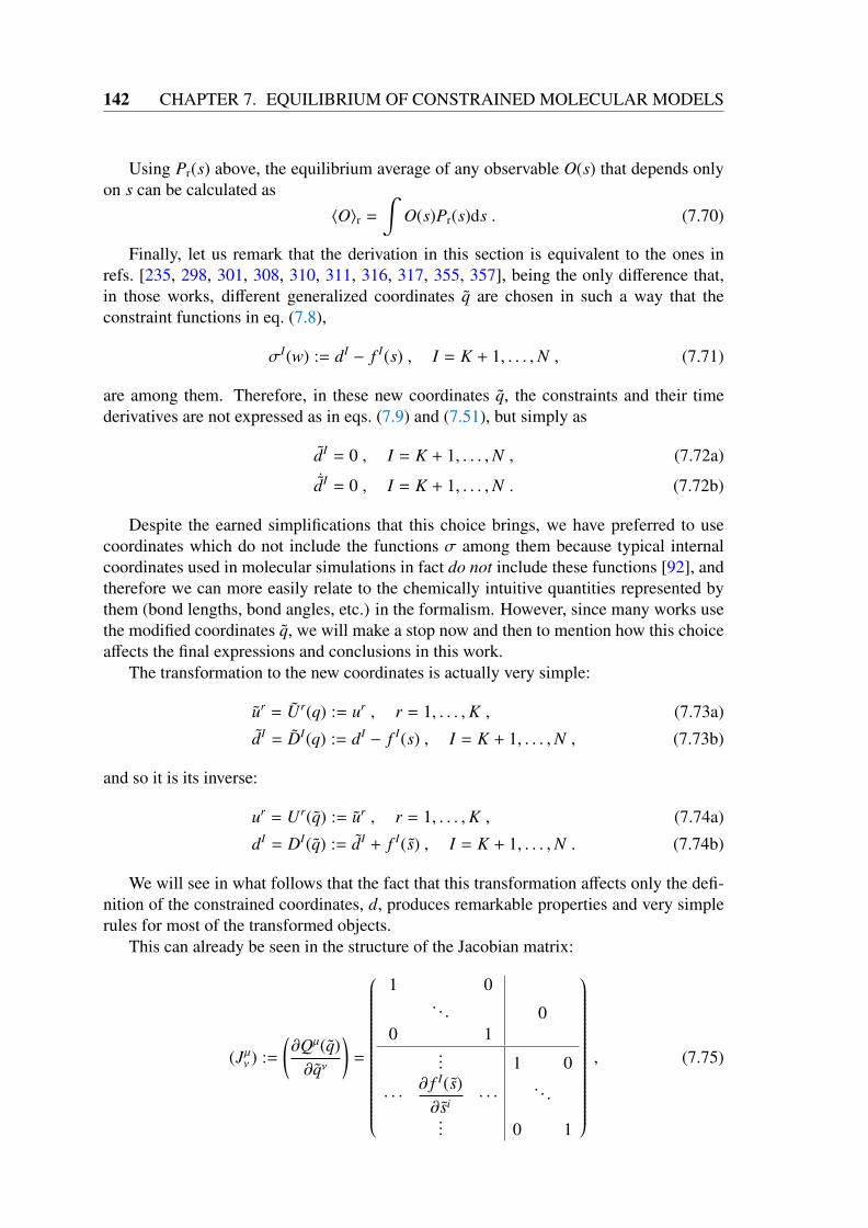
142 CHAPTER 7. EQUILIBRIUM OF CONSTRAINED MOLECULAR MODELS
Using Pr(s) above, the equilibrium average of any observable O(s) that depends onlyon s can be calculated as
〈O〉r =
∫O(s)Pr(s)ds . (7.70)
Finally, let us remark that the derivation in this section is equivalent to the ones inrefs. [235, 298, 301, 308, 310, 311, 316, 317, 355, 357], being the only difference that,in those works, different generalized coordinates q are chosen in such a way that theconstraint functions in eq. (7.8),
σI(w) := dI − f I(s) , I = K + 1, . . . ,N , (7.71)
are among them. Therefore, in these new coordinates q, the constraints and their timederivatives are not expressed as in eqs. (7.9) and (7.51), but simply as
dI = 0 , I = K + 1, . . . ,N , (7.72a)˙dI = 0 , I = K + 1, . . . ,N . (7.72b)
Despite the earned simplifications that this choice brings, we have preferred to usecoordinates which do not include the functions σ among them because typical internalcoordinates used in molecular simulations in fact do not include these functions [92], andtherefore we can more easily relate to the chemically intuitive quantities represented bythem (bond lengths, bond angles, etc.) in the formalism. However, since many works usethe modified coordinates q, we will make a stop now and then to mention how this choiceaffects the final expressions and conclusions in this work.
The transformation to the new coordinates is actually very simple:
ur = Ur(q) := ur , r = 1, . . . ,K , (7.73a)
dI = DI(q) := dI − f I(s) , I = K + 1, . . . ,N , (7.73b)
and so it is its inverse:
ur = Ur(q) := ur , r = 1, . . . ,K , (7.74a)
dI = DI(q) := dI + f I(s) , I = K + 1, . . . ,N . (7.74b)
We will see in what follows that the fact that this transformation affects only the defi-nition of the constrained coordinates, d, produces remarkable properties and very simplerules for most of the transformed objects.
This can already be seen in the structure of the Jacobian matrix:
(Jµν ) :=(∂Qµ(q)∂qν
)=
1 0. . . 0
0 1... 1 0
· · ·∂ f I(s)∂si · · ·
. . .
... 0 1
, (7.75)

7.2. THEORETICAL FRAMEWORK AND RELATION TO PREVIOUS WORKS 143
and its inverse:
((J−1)µν
):=
(∂Qµ(q)∂qν
)=
1 0. . . 0
0 1... 1 0
· · · −∂ f I(s)∂si · · ·
. . .
... 0 1
, (7.76)
both of which have unit determinant: det J = det J−1 = 1.It is also worth mentioning that, if the constraints are defined as hard (see the next
section), then the σ functions in eq. (7.71) become
σI(w) := dI − dI0 , I = K + 1, . . . ,N , (7.77)
being dI0 constant numbers, and in such a case the simplicity of the change of coordinates
is even higher, being the Jacobian and its inverse in the expressions above both exactlyequal to the identity matrix.
In any case, either if the generalized velocities are related as in eq. (7.51) or if theyare zero as in eq. (7.72b) and in refs. [235, 298, 301, 308, 310, 311, 316, 317, 355, 357],it is convenient to bear in mind that momenta and velocities are only proportional whenthe matrix in the kinetic energy is diagonal (e.g., in Euclidean coordinates ), and thestatement sometimes found in the literature [246, 302, 305, 313, 355, 359, 360] about thecancelation of the momenta associated to the constrained coordinates is wrong in general.
Regarding the calculations in this section, the use of the modified coordinates q leadsto a simpler expression for the induced MMT in eq. (7.53):
grs(u) = GKrs(u) , (7.78)
i.e., it is simply the unconstrained-unconstrained block of the whole-space MMT G eval-uated in the constrained subspace (see sec. 7.2.5 for the implications of this in the calcu-lation of Fixman’s potential).
Moreover, if we use eq. (7.109) for the transformation of the whole-space MMT Gtogether with the change of coordinates in eq. (7.74), we can prove that
grs(u) = GKrs(u) := Grs(u, 0)
= Grs(Q(u, 0)
)+∂ f I(u)∂ur GIs
(Q(u, 0)
)+ GrJ
(Q(u, 0)
)∂ f J(u)∂us
+∂ f I(u)∂ur GIJ
(Q(u, 0)
)∂ f J(u)∂us
= Grs(u, f (u)
)+∂ f I(u)∂ur GIs
(u, f (u)
)+ GrJ
(u, f (u)
)∂ f J(u)∂us
+∂ f I(u)∂ur GIJ
(u, f (u)
)∂ f J(u)∂us = grs(u) , (7.79)
i.e., the induced MMT is not modified upon the change of coordinates from q to q; it isthe same as the original one component-wise.

144 CHAPTER 7. EQUILIBRIUM OF CONSTRAINED MOLECULAR MODELS
This directly implies that the calculations associated to the factorization and elimina-tion of the external coordinates in ref. [255], which led us to expressions (7.64), (7.65),and related quantities, still apply in the new modified coordinates. The only change to bedone is to place a ‘tilde’ over the appropriate symbols.
Rigid model with hard constraints
As already mentioned, the most common constrained dynamics considered in the litera-ture is not the rigid one with flexible constraints described in the previous section, but theone with hard constraints. This option, which is numerically simpler, and which can beaccurate enough for certain applications, is described in the following paragraphs.
The key difference between the two models is that, in the hard case, the constrainedcoordinates d are not equal to some functions f (s) of the unconstrained internal coordi-nates, as expressed in eq. (7.9), but to some constant numbers d0:
dI = dI0 , I = K + 1, . . . ,N . (7.80)
This makes all partial derivatives in eqs. (7.51) and (7.53) zero, and converts the in-duced MMT g(u) simply in the unconstrained-unconstrained sub-block of the restrictionto K of the whole-space MMT, i.e.,
grs(u) = GKrs(u) := Grs(e, s, d0) , (7.81)
where we have used an over-bar to denote hard objects. This fact has important impli-cations regarding the Fixman’s compensating potential, introduced in sec. 7.2.5. Alsonotice, that, contrarily to eq. (7.78), which only held in the flexible case if the modifiedcoordinates q were used, we now have this property in the original molecular coordinatesq.
Another, more subtle consequence of the use of hard constraints affects the calcula-tions of the partial derivatives ∂R ′α/∂si, which are a key ingredient of the matrix g ′(s) ineq. (7.65). If we realize that the functions R ′α (s) are implicitly defined in eq. (7.10) as
R′α (s) := ~R ′α
(s, f (s)
), (7.82)
the sought derivatives can be computed using
∂R ′α∂si (s) =
∂~R ′α∂si
(s, f (s)
)+∂~R ′α∂dI
(s, f (s)
)∂ f I
∂si (s) . (7.83)
In the flexible case, all terms in the sum are in principle non-zero, and the fact that thederivatives ∂ f I/∂si must be typically found numerically requires the use of complicatedalgorithms to obtain this quantities (see sec. 7.3 and chapter 6). In the hard case, on theother hand, all these derivatives are zero and eq. (7.83) reduces to
∂R ′α∂si (s) =
∂~R ′α∂si (s, d0) , (7.84)
which contains only explicit derivatives which can typically be computed analytically.The efficient calculation of the MMT, MMT determinants, and related quantities in refs. [303,
7.2. THEORETICAL FRAMEWORK AND RELATION TO PREVIOUS WORKS 145
306, 314, 315, 351, 354, 355], where they consider only hard constraints, is implicitlybased on this fact.
Apart from these (important) differences, the dynamics of the rigid model with hardconstraints is derived following the same steps we took in the previous section, and therigid Hamiltonian in eq. (7.49) is still applicable to this case as long as we compute theinduced MMT as indicated in eq. (7.81). This dynamics can be implemented in a computerusing many different algorithms (see refs. [237, 298, 307], and references therein; andalso [366] in this special issue), and, again, under the usual assumptions of ergodicity andequal a priori probabilities, its Statistical Mechanics equilibrium can be described in aformally identical way to the flexible case, via eqs. (7.68), (7.69a) and (7.69b).
Despite this formal identity, however, it has been shown that the flexible and hard dy-namics produce different physical results (see refs. [242–244, 301, 367] and also sec. 7.3),and indeed in sec. 7.2.3 we built a strong case for considering the latter as an approxima-tion of the former. In sec. 7.3, we will additionally illustrate how this difference in thedynamics produce measurable discrepancies at the level of equilibrium Statistical Me-chanics in a methanol molecule.
Stiff model with flexible constraints
In the previous two sections, we discussed the dynamics as well as the canonical equilib-rium of the so-called rigid model, in which not only the constraints are assumed to holdexactly but also D’Alembert’s principle, which hypothesizes that the components of theforces of constraint tangent to the constrained subspace Σ are zero [249, 312].
Nevertheless, if we accept the unconstrained dynamics as the reference against whichto assess the accuracy of any approximate model (see the discussion supporting this choicein sec. 7.2.3), we must realize that, if the system is in contact with a thermal bath attemperature T , even if there exist strong forces that drive it to the constrained subspaceΣ, there also exist random fluctuations that will inevitably take the system away from thisregion. Moreover, even in the case in which we can assume that the potential energyoutside Σ tends to infinity (a case in which the constraints hold exactly by simple energyconservation arguments [368]), it can be proved that the force on Σ resulting from thislimit procedure not only consists of the orthogonal component needed to keep the systemin the constrained subspace, but also of a non-zero tangent component that must be addedto the expected gradient of VΣ(s), i.e., D’Alembert’s principle, even in the infinitely steepconfining potential case, is not satisfied in general [248, 283, 312, 324, 334, 369].
These two in general violated assumptions confirm what we already suspected: thatthe rigid dynamics and Statistical Mechanics equilibrium are just an approximation of thereal, unconstrained ones (even if we use the more physically sound flexible constraints).Therefore, if the rigid dynamics is to be used in practical simulations in order to gain theadvantages discussed in sec. 9.1, it becomes necessary to assess how much error theseapproximations introduce.
Of course, in order to compare the rigid Statistical Mechanics equilibrium PDF Pr(s)in eq. (7.68) to the unconstrained one in P(w) in eq. (7.32) (or the free energies in theirrespective exponents), we should arrive to some objects that are defined on the samespace, being the most natural candidates Pr(s) itself and the marginal unconstrained PDFin the space, Σ, spanned by the unconstrained internal coordinates s. This last function is

146 CHAPTER 7. EQUILIBRIUM OF CONSTRAINED MOLECULAR MODELS
obtained through the integration of the constrained coordinates d as usual:
P(s) :=∫
P(w)dd . (7.85)
However, in the general case this is only formal, i.e., for a general potential V(w) andgeneral curvilinear coordinates q, this integral cannot be calculated analytically. One ofthe available options is to compute it numerically, with the help of methods for calculatingfree energy differences [235, 276, 277, 370, 371]. In this work, on the other hand, we havechosen to develop a statistical mechanics model, termed stiff, whose effective free energyin Σ can be analytically obtained and compared to the rigid one in a more direct andinsightful way than the result of numerically performing the integral in eq. (7.85), at thesame time that it could be considered an approximation to the unconstrained equilibriumcontaining weaker assumptions than the rigid one. Contrarily to the rigid model, the stiffone does account for the statistical weights of the conformations close to (but out of) Σ,at the same time that it allows for the existence of velocities that are orthogonal to theconstrained subspace. Also, in the derivation of the stiff model, D’Alembert’s principleis never invoked. These arguments, together with the knowledge of the controlled stepsthat take us from the unconstrained case to the stiff model, suggest that one could expectthe stiff equilibrium to be closer to the unconstrained one than the rigid equilibrium notonly conceptually but also in quantitative terms. Although in this chapter we will assumethis to be true and the stiff model will be used as the reference against which to assessthe accuracy of any constrained model, numerical confirmation will be pursued in futureworks.
The first step in the derivation of the stiff model consists of Taylor expanding thepotential energy V(s, d) at a fixed point s, in terms of the constrained coordinates d, aroundthe point d = f (s):
V(s, d) = V(s, f (s)
)+
[∂V∂dI
(s, f (s)
)] (dI − f I(s)
)(7.86)
+12
[∂2V∂dI∂dJ
(s, f (s)
)] (dI − f I(s)
)(dJ − f J(s)
)+ O
((d − f (s)
)3),
or, realizing that to evaluate in(s, f (s)
)is to evaluate in the internal constrained subspace
Σ,
V(s, d) = VΣ(s) + ∂IVΣ(s)(dI − f I(s)
)(7.87)
+12HΣ
IJ(s)(dI − f I(s)
)(dJ − f J(s)
)+ O
((d − f (s)
)3),
where we have used the notation for the constrained Hessian in eq. (7.44), and we haveintroduced the notation ∂IVΣ(s) for the gradient of V(w) restricted to Σ.
The same expansion can be performed on S k(w), yielding
S k(s, d) = S kΣ(s) + ∂IS k
Σ(s)(dI − f I(s)
)(7.88)
+12∂2
IJS kΣ(s)
(dI − f I(s)
)(dJ − f J(s)
)+ O
((d − f (s)
)3),

7.2. THEORETICAL FRAMEWORK AND RELATION TO PREVIOUS WORKS 147
and both of them can be introduced into the integral that appear in the definition of themarginal PDF in eq. (7.85):
P(s) :=∫
P(w)dd =
∫e−β[V(w)−TS k(w)]dd∫
e−β[V(w ′)−TS k(w ′)]ds ′dd ′. (7.89)
Note that expanding the term associated to the determinant of the whole-space MMTdet G in the marginal PDF in positions space is in principle more accurate that the pro-cedure followed in refs. [233, 298, 308, 310, 311, 316–318, 355, 356, 372] or in ourown work in ref. [240], where the dependence of det G on the constrained coordinatesd is simply neglected, evaluating this determinant directly in d = f (s) and thus effec-tively truncating the expansion in eq. (7.88) at zero order (often implicitly). In fact, thispoint and the inclusion of flexible constraints in the mix are the only issues that make theformalism in this work more general than the ones in refs. [240, 308, 310, 311, 316, 317].
Now, if we assume that the constrained coordinates are indeed “stiff”, i.e., that, asmentioned in sec. 7.2.3, for “small” variations ∆d in d, we have V
(s, f (s)+∆d
)−V
(s, f (s)
)
RT , then the quantities under the integral signs, which are proportional to e−V(s,d)/RT , willbecome negligibly small as soon as we separate from the constrained subspace Σ by anyrelevant amount. Moreover, we also know that, close to Σ, the Taylor expansions ineqs. (7.87) and (7.88) can be truncated at low order. Therefore, for each fixed value ofthe unconstrained coordinates s, we can substitute the potential energy and the kineticentropy terms by their respective low-order Taylor expansions. Also note that this verysame argument can be used if we had chosen to define Σ through the minimization of F(q)instead of V(w).
In principle, there is no reason to truncate at different orders the potential energyV(s, d) and the kinetic entropy S k(s, d).
If we truncate both expansions at order zero, we simply have that the exponentialdoes not depend on the constrained coordinates, and the integral
∫1dd cancels out in the
numerator and the denominator of eq. (7.32), yielding the (0,0)-stiff PDF in Σ:
P(0,0)s (s) =
e−βF(0,0)s (s)∫
e−βF(0,0)s (s ′)ds ′
, (7.90)
where we have defined
F(0,0)s (s) := VΣ(s) − TS k
Σ(s) , (7.91a)
S kΣ(s) :=
R2
ln det G ′Σ (s) , (7.91b)
being G ′Σ
(s) the restriction to Σ of the matrix G ′(w).Although this Statistical Mechanics model is well-defined and may be certainly con-
sidered for some applications (in sec. 7.2.5 we mention a number of works in which it hasbeen implicitly used), two issues lead to try to improve it: On the one hand, the truncationof the Taylor expansions at order zero means that we are only looking at points exactly onΣ, and not “close” to it, which was one of the weaknesses, we argued, of the rigid model.On the other hand, the function we are substituting V(s, d) with, i.e., VΣ(s), does not havethe important property of becoming very large when the constrained coordinates get away
148 CHAPTER 7. EQUILIBRIUM OF CONSTRAINED MOLECULAR MODELS
from Σ (because it does not depend on them!). The fact that we could obtain a finite PDF,P(0,0)
s (s), is attributable to the cancellation of an infinite quantity61,∫
1dd, in the numeratorand the denominator. However, if we consider the partition function of the system afterperforming the substitution, Z =
∫e−β(VΣ(s)−TS k
Σ(s))dsdd, we see that it is infinite, which is
certainly a warning and probably a problem.If we truncate both expansions at the first order, and we assume that we are dealing
with flexible constraints defined by the functions f (s) taking the values of the constrainedcoordinates that minimize the potential energy at point s, then the first derivatives ∂IVΣ(s)are zero, and the leading order in the expansion of V(s, d) is again VΣ(s). Therefore,for the (1,1)-stiff model, the exponent in the integral is proportional to VΣ(s) − TS k
Σ(s) −
T∂IS kΣ(s)
(dI − f I(s)
), and, since the sign of the terms ∂IS k
Σ(s) can be anyone, there is no
reason for the integral on the constrained coordinates to be convergent. If we consideredthe definition of Σ involving the minimization not of V(w) but of F(q), the situation isslightly different but simple, since in this case ∂IVΣ(s) − T∂IS k
Σ(s) = 0, and the (1,1)-stiff
model would be equivalent to the (0,0) one.It becomes then clear that the second order terms must be included in the model if
we want to work with finite quantities. Truncating both expansions at second order, andusing eq. (7.25), we find the most general expression for the integral over the constrainedcoordinates that will be considered in this work:∫
exp[− β
(VΣ − TS k
Σ + (∂IVΣ − T∂IS kΣ)(dI − f I)
+12
(dI − f I)AIJ(dJ − f J))]
dd (7.92)
=
(2πβ
) L2
det−12 A exp
[β2
(∂IVΣ − T∂IS kΣ)AIJ(∂JVΣ − T∂JS k
Σ)],
where we have omitted the dependence on s, and we have defined
AIJ := HΣIJ − T∂2
IJS kΣ , (7.93)
in order to lighten the notation. We have also approximated the different ranges of inte-gration of the constrained coordinates all by the (−∞,∞) range (notice that bond lengthsrange from 0 to∞, bond angles from 0 to π, etc.). The reason why this is expected to be agood approximation is the same that supports the rest of the calculations, namely, that theintegrated quantity is only non-negligible close to the constrained subspace Σ, where theconstrained coordinates are typically far away from the true integration limits.
Despite this formal result, one needs to notice that, for the above integral to exist, thematrix A has to be positive definite. If we had chosen the definition of the constrainedsubspace based on the minimization of F(q), this property would be satisfied, since A isprecisely the Hessian of F(q) at a minimum. In the case treated here, however, the positivedefiniteness of A is not guaranteed. If we are in a minimum of the potential energy, theconstrained Hessian HΣ
IJ in eq. (7.44) is indeed positive definite, but the presence of theterm −T∂2
IJS kΣ
spoils this property, in general, for the matrix A. If such a thing happens,or even if it is “close” to happening (for example, if the smallest eigenvalue of A becomes
61 At least if any bond length is included among the constrained coordinates, which is always the case inpractical applications.

7.2. THEORETICAL FRAMEWORK AND RELATION TO PREVIOUS WORKS 149
too close to zero), we must consider the possibility of moving to the model based on theminimization of F(q).
Another issue that may cause the eigenvalues of the matrix A to be small and thusrender the stiff approximation questionable is that the coordinates we have selected asconstrained may actually be a bad choice. Indeed, if the statistical weights of the confor-mations do not become significantly small as we move away from Σ at second order in theunconstrained free energy F(w) := V(w) − TS k(w), then we have little reasons to believethat the situation might change if we include higher orders. Hence, although the (2,2)-stiffmodel might not be a very good approximation at every point s, we should see the positivedefiniteness of the matrix A in eq. (7.93) and the size of its eigenvalues as a consistencycheck, and regard those points at which these conditions fail as points in which the (2,2)-stiff model is a bad approximation of the unconstrained equilibrium, and the constrainedcoordinates are probably not “stiff” enough. Although we have not found conformationsin which A (or H ; see below) contains negative eigenvalues in the practical example insec. 7.3, this is probably so because of the small size of the molecule studied. For largersystems, we have already seen some preliminary indications that these matrices might infact become not positive definite depending on the chosen constrained coordinates.
Now, using eq. (7.92) and recalling that the first derivatives of the potential energyrestricted to Σ are zero in the chosen model, we have that the (2,2)-stiff PDF in Σ is givenby
P(2,2)s (s) =
e−βF(2,2)s (s)∫
e−βF(2,2)s (s ′)ds ′
, (7.94)
with
F(2,2)s (s) := VΣ(s) − TS k
Σ(s) − TS cA(s) −
T 2
2∂IS k
Σ(s)AIJ(s)∂JS kΣ(s) , (7.95)
being AIJ the entries of A−1 and
S cA(s) := −
R2
ln det A(s) , (7.96)
where the letter “c” in the new entropy stands for conformational, in reference to the factthat it appears as the result of eliminating some positions, and not momenta, being rem-iniscent of the conformational or configurational entropies appearing in quasi-harmonicanalysis [318, 319, 373]. The only difference that we would find if we chose the definitionbased on the minimization of F(q) is that the last term in eq. (7.95) would not appear. Aswe mentioned, the (2,2)-stiff model is the most general stiff model in this work and it hasnever been used before in the literature as far as we know.
The calculation of HΣ(s), which appears in A(s), can be performed in many differentways depending on the potential energy we are dealing with (the computation of the otherpart of A is described later). The calculation of det G ′
Σ(s), on the other hand, is entirely
“geometric”, depending only on the scheme of internal coordinates chosen to describe thesystem (assuming that the functions f (s) have already been calculated). The way to com-pute det G ′(w) analytically has been described before, using the analogue of eq. (7.65)but without constraints. However, if a specific set of internal coordinates is chosen, onecan arrive to a much simpler and more explicit expression. In our work in ref. [255], we

150 CHAPTER 7. EQUILIBRIUM OF CONSTRAINED MOLECULAR MODELS
showed that, if the SASMIC internal coordinates [92] for general branched molecules areused (a similar result will hold for any well-designed scheme of internal coordinates), wehave that
det G ′(w) =
n∏α=1
m3α
n∏α=2
l4α
n∏α=3
sin2θα
, (7.97)
where lα are the bond lengths, and θα the bond angles associated to atom α. The massescan be eliminated, since they come out of the logarithm as an additive term, which rep-resents a constant change of reference in the free energy, and has no effect whatsoeverin the equilibrium PDF. Go and Scheraga also proved this result long ago using differentmathematics [250].
This expression, together with the additivity of the logarithm, not only helps to easilycalculate S k(w) [and therefore its restriction S k
Σ(s)], but also its derivatives with respect to
any internal coordinate depending on its type:
∂S k
∂lα(w) =
2Rlα
, (7.98a)
∂S k
∂θα(w) = R cotg θα , (7.98b)
∂S k
∂φα(w) = 0 , (7.98c)
where φα denotes the dihedral angle associated to atom α.Using these results, we can rewrite eq. (7.95) as
F(2,2)s (s) := VΣ(s) − TS k
Σ(s) − TS cA(s) + U (2)
s (s) , (7.99)
withU (2)
s (s) := −1
2β2 D(f I(s)
)AIJ(s)D
(f J(s)
), (7.100)
being D(dI) the function defined as
D(dI) :=
2/dI if dI is a bond lengthcotg dI if dI is a bond angle0 if dI is a dihedral angle
. (7.101)
The entries, ∂2IJS k(w), of the matrix whose restriction to Σ appears in the definition of
A in eq. (7.93) can also be easily computed, yielding
T∂2IJS k(w) = −
1βδIJD2(dI) , (7.102)
where δIJ is the Kronecker’s delta, and D2(dI) is the function defined as
D2(dI) :=
2/(dI)2 if dI is a bond length1/ sin2 dI if dI is a bond angle0 if dI is a dihedral angle
, (7.103)

7.2. THEORETICAL FRAMEWORK AND RELATION TO PREVIOUS WORKS 151
allowing to rewrite eq. (7.93) as
AIJ(s) := HΣIJ(s) +
1βδIJD2
(f I(s)
). (7.104)
Note that both D(dI) and D2(dI) are singular only in points that have little physicalmeaning and that will be never reached in a practical simulation: lα = 0 or θα = 0, π.Not only the energy will be very large (even infinite) at these points, but also the changeof coordinates in eq. (7.1) from the Euclidean to the curvilinear coordinates becomessingular.
Apart from the (2,2)-stiff model, we can also define two other models which yieldconvergent integrals for any point s. However, they are derived truncating the potentialenergy and the kinetic entropy at different orders; something which is, in principle, notjustified.
Particularizing eq. (7.92), we have that the (2,0)-stiff effective free energy is given by
F(2,0)s (s) := VΣ(s) − TS k
Σ(s) − TS cH
(s) , (7.105)
withS cH
(s) := −R2
ln detHΣ(s) . (7.106)
As we discuss in sec. 7.2.5, this model has been implicitly used in some works, in-cluding one by some us [240].
The (2,1)-stiff free energy, in turn, includes an additional term:
F(2,1)s (s) := VΣ(s) − TS k
Σ(s) − TS cH
(s) + U (1)s (s) , (7.107)
defined asU (1)
s (s) := −1
2β2 D(dI(s)
)H IJ
Σ (s)D(dJ(s)
), (7.108)
where we have used again that the first derivatives of the potential energy are zero in Σ,and H IJ
Σ(s) are the entries of the inverse matrix of the constrained Hessian, as usual. If
the definition of the constrained subspace based on the minimization of F(q) is used, thenthe (2,0)- and (2,1)-stiff models become identical.
Now, if the modified coordinates q defined in sec. 7.2.4 are used in the calculationsin this section, several points need to be re-examined. First of all, we have the follow-ing relationship between the whole-space MMT in the coordinates q and the one in thecoordinates q (indeed, we have it for any 2-times covariant tensor [238]):
Gµν(q) =∂Qρ(q)∂qµ
Gρσ
(Q(q)
)∂Qσ(q)∂qν
. (7.109)
Hence, if we use the fact that the determinant of a product of square matrices is theproduct of the determinants, and also the property mentioned in sec. 7.2.4 about the Jaco-bian determinant of the change of coordinates being 1, we have that
det G(q) = det G(Q(q)
). (7.110)
Note that this not only guarantees the factorization of the external coordinates ineq. (7.31), but it also allows us to use the explicit expression (7.97) in terms of the molec-ular coordinates q to compute det G(q) as long as we insert the transformation functions

152 CHAPTER 7. EQUILIBRIUM OF CONSTRAINED MOLECULAR MODELS
Q(q) into the appropriate functional places corresponding to bond lengths and bond an-gles.
Also using the structure of the Jacobian in eq. (7.75), it is easy to prove that thetransformed potential energy,
V(q) := V(Q(q)
), (7.111)
and indeed any scalar function (such as det G above, and hence S k), satisfies
∂V∂dI
(q) =∂V∂dI
(Q(q)
), (7.112)
as well as∂2V∂dI∂dJ
(q) =∂2V∂dI∂dJ
(Q(q)
). (7.113)
These transformation rules guarantee that all the final expressions in this section areidentical in the case that we wished to use the modified coordinates q, as long as we“place tildes” over all relevant objects, such as H(q), A(q) or S k(q). But not only that,they also allow us to compute the objects in the original coordinates q and then simplyperform the substitution Q(q) to find the transformed quantities. This is very convenient,since the coordinates q are defined in terms of the functions f (s), which are typicallyimpossible to express analytically, while the coordinates q are simple functions of theEuclidean coordinates, thus admitting compact algorithms for computing quantities suchas the Hessian of the potential energy, or the functions D(d) and D2(d) in eqs. (7.101)and (7.103), respectively.
It is also worth remarking that, in the derivation of the stiff models in the coordinatesq, the Taylor expansion of the potential energy in eq. (7.86) would be performed at d = 0and take the simpler form
V(s, d) = V(s, 0) +
[∂V∂dI
(s, 0)]
dI +
[∂2V∂dI∂dJ
(s, 0)]
dI dJ + O(d3) , (7.114)
which allows to make contact with some of the potential energy functions in previousworks [245, 301, 308, 311, 316, 317], realizing that the intention of the authors may notbe to restrict themselves to a particular case of the completely general potential consideredhere, but just that they are using the modified coordinates q, instead of the molecular coor-dinates q used in this work. See however the discussion in sec. 7.2.5, about the neglectionof the dependence of the Hessian on s, which is not a general feature of eq. (7.114),irrespective of the coordinates used.
Finally, to close this section, let us raise an important and subtle point related to thestiff model and the dynamics of the system: As we have emphasized in previous sections,the analysis presented in this work is completely at the equilibrium Statistical Mechanicslevel; all approximations are performed in equilibrium PDFs and all constrained mod-els are defined in these terms too. In the previous rigid sections, we briefly commentedthat the rigid equilibrium can be sampled using available dynamical algorithms such asSHAKE [237, 298, 366] or any of its more modern descendants (see ref. [307] and refer-ences therein) for the hard case; and the algorithms in refs. [241–243] if the constraints areflexible. That this sampling can be achieved by such algorithms is easily understandableif we recall that the rigid model is obtained from a Hamiltonian [the one in eq. (7.49)]

7.2. THEORETICAL FRAMEWORK AND RELATION TO PREVIOUS WORKS 153
and thus the corresponding discretized Hamilton equations (properly thermostated [337])will do the trick. Moreover, the fact that the fastest vibrations are absent from this dy-namics makes the integration algorithms potentially more efficient than the unconstraineddynamics, and the whole scheme is thus useful.
In the case of the stiff model introduced in this section, the situation is entirely differ-ent. We may of course ask the theoretical question of which would be a dynamics thatdirectly samples the stiff Statistical Mechanics equilibrium, and we may even find somedynamics that do the job. However, any naive version of such a dynamics will in principlecontain the fast vibrations that we sought to eliminate with the use of constraints, andtherefore any algorithm that implements it would probably be as numerically costly asthe whole unconstrained dynamics (at least). Since the only rationale behind the develop-ment of the stiff model was to provide a good approximation to the unconstrained systemin order to be able to assess the accuracy of the rigid equilibrium, using a new “stiff”dynamics instead of the unconstrained one itself seems a rather unprofitable (and convo-luted) enterprise. In principle, the stiff model should be regarded as an approximation tothe unconstrained equilibrium at the level of Statistical Mechanics, not at the level of thedynamics. However, as we will discuss in sec. 7.2.5, there is a way of sampling the stiffequilibrium using a rigid dynamics with an additional correcting term (see fig. 7.2 for aschematic summary of these ideas). Whether or not the calculation of this correcting termcan be performed fast enough so that we end with a dynamics which has the accuracy ofthe stiff model while retaining the efficiency of the rigid one is, however, a topic that wewill not analyze in depth in this work.
Stiff model with hard constraints
In principle, we can also consider the stiff model defined using the hard constraints ineq. (7.80). The main difference with the flexible case appears in the Taylor expansions ineq. (7.87) and (7.88), which become
V(s, d) = VΣ(s) + ∂IVΣ(s)(dI − dI0) (7.115)
+12HΣ
IJ(s)(dI − dI0)(dJ − dJ
0) + O((d − d0)3) ,
and
S k(s, d) = S kΣ(s) + ∂I S k
Σ(s)(dI − dI0) (7.116)
+12∂2
IJS kΣ(s)(dI − dI
0)(dJ − dJ0) + O
((d − d0)3) ,
where we have used again an over-bar to distinguish objects associated to the hard con-straints from their flexible counterparts (meaning they are evaluated at d = d0 instead ofd = f (s)).
Also, since the values d = d0 do not need to minimize the potential energy at the points [nor the free energy F(q)], the derivatives ∂IVΣ(s), ∂I S k
Σ(s) and ∂IVΣ(s) − T∂I S k
Σ(s) are
all non-zero in general, and neither the Hessian HΣ(s) nor the associated matrix A(s) areguaranteed to be positive definite in the hard case.
All calculations for the hard stiff models are formally identical to the ones in theprevious section as long as we include the terms ∂IVΣ(s) and ∂I S k
Σ(s), and substitute the
functions f (s) by the constant values d0.

154 CHAPTER 7. EQUILIBRIUM OF CONSTRAINED MOLECULAR MODELS
In particular, the hard (2,2)-stiff model has free energy
F(2,2)s (s) := VΣ(s) − TS k
Σ(s) − TS cA(s) + U (2)
s (s) , (7.117)
with
S kΣ(s) :=
R2
ln det G ′Σ (s) , (7.118a)
S cs(s) := −
R2
ln det A(s) , (7.118b)
and
U (2)s (s) := −
12
(∂IVΣ(s) −
D(dI0)
β
)AIJ(s)
(∂JVΣ(s) −
D(dJ0)
β
),
being
AIJ(s) := HΣIJ(s) +
1βδIJD2(dI
0) . (7.119)
As in the flexible case, the substitution of the second order expansion of the free energyinto the integral in eq. (7.89) is only justified if A is positive definite and has large enougheigenvalues. In the case of the hard (2,2)-stiff model, the failure of such a property can becaused not only by the fact that the chosen constrained coordinates are actually not very“stiff” or because we have decided to minimize V(w) instead of F(q) (as it happened forthe flexible case in the previous section), but also because of having expanded around avalue, d0, which is not a minimum of the potential energy [or of F(q)], thereby possiblydistorting the observed curvature encoded in HΣ and A.
The only hard stiff model that presents an equilibrium PDF that is convergent for allpoints s (but a partition function that is infinite) is the (0,0)-stiff model, whose free energyis given by
F(0,0)s (s) := VΣ(s) − TS k
Σ(s) . (7.120)
As in the flexible case, the first order truncation produces models that are, in general,non-convergent, while we can still define two models that may be well-behaved dependingon the properties of the hard constrained Hessian HΣ: the (2,0)- and (2,1)-stiff models.Notice, on the one hand, that these two models were convergent at all points s in theflexible case, because the flexible constrained Hessian is, by construction, positive defi-nite. On the other hand, the same caution applies in the hard case regarding the a priorijustification of truncating the potential energy V(s, d) and the kinetic entropy S k(s, d) atdifferent orders.
The hard (2,0)-stiff model has free energy
F(2,0)s (s) := VΣ(s) − TS k
Σ(s) − TS cH
(s) + U (0)s (s) , (7.121)
with
U (0)s (s) := −
12∂IVΣ(s)H IJ
Σ (s)∂JVΣ(s) , (7.122)
and
S cH
(s) := −R2
ln det HΣ(s) , (7.123)

7.2. THEORETICAL FRAMEWORK AND RELATION TO PREVIOUS WORKS 155
Figure 7.2: Summary and relationships among the models discussed in this work. Fora precise definition of the different mathematical objects and the meaning of the models,see the main body of the chapter.
whereas the free energy of the hard (2,1)-stiff model is given by
F(2,0)s (s) := VΣ(s) − TS k
Σ(s) − TS cH
(s) + U (1)s (s) , (7.124)
being
U (1)s (s) := −
12
(∂IVΣ(s) −
D(dI0)
β
)H IJ
Σ (s)(∂JVΣ(s) −
D(dJ0)
β
). (7.125)
It is also worth noting here that, in the hard case treated in this section, there is nodifference between minimizing V(w) or F(q), because the constrained subspace is notdefined through any minimization, but it is postulated to simply be d = d0.
Some of these models have been implicitly used in the literature before, as we mentionin the next section. In fact, being the hard constraints more popular, their use have beenmore common than that of their flexible counterparts in sec. 7.2.4.
7.2.5 Summary, comparisons and the Fixman’s potentialIn fig. 7.2, a schematic depiction of the models discussed in the previous sections canbe found, together with the relationships among them, as well as the basic mathemati-cal expressions used to describe their respective Statistical Mechanics in the constrainedsubspace. In the figure, only the flexible versions of the constrained models have beendetailed, and only the more accurate (2,2)-type of stiff model is shown. An equivalentscheme will be obtained if we define the constrained subspace Σ using the hard relationsd = d0 or we truncate the Taylor expansions defining the stiff model at a different orderthan 2.

156 CHAPTER 7. EQUILIBRIUM OF CONSTRAINED MOLECULAR MODELS
In words, we have the unconstrained dynamics, which, we have argued, is the refer-ence to which we will judge the accuracy of any constrained model. On the other end ofthe scheme, we have the rigid dynamics, which is potentially faster than the unconstrainedone because the fastest vibrations have been eliminated from the system by constrainingthe associated degrees of freedom. Despite this better numerical profile, the rigid dy-namics, and its corresponding Statistical Mechanics equilibrium in the constrained sub-space Σ are based on some questionable assumptions, such as D’Alembert’s principle,or the imposition that the dynamics takes place exactly on Σ, thus forbidding the systemto present velocities that are orthogonal to this space. These strong approximations re-quire that we assess the accuracy of the rigid model against the reference unconstrainedsituation. In this work, we choose to do so at the level of equilibrium Statistical Me-chanics, where the key object is the PDF and the free energy that appears in its exponent.Given the typical complexity of molecular potential energy functions, the integral neededto marginalize the unconstrained PDF to the constrained subspace Σ and thus be able tocompare it with the rigid one is too complicated to be performed analytically. This iswhy we have introduced an approximation to the unconstrained equilibrium, which hasΣ as its natural probability space, which is based on weaker assumptions than the rigidmodel, and which is termed stiff model. Now, by comparing the rigid equilibrium tothe stiff one, the accuracy of the former can be assessed. That they are indeed appre-ciably different has long be known in the literature and many works have discussed it[8, 233, 246, 248, 250, 284, 290, 298, 303–306, 308–311, 313–317, 355, 359, 374].
The most natural way to perform this assessment is to compare the two effective freeenergies that appear in the exponents of their respective PDFs. For example, if we considerthe more general case of flexible constraints, and we use the most accurate (2,2)-stiffmodel, we can define the following function of the unconstrained coordinates s:
VF(s) := F(2,2)s (s) − Fr(s) = TS k
r (s) − TS kΣ(s) − TS c
A(s) + U (2)s (s) , (7.126)
which quantifies the difference between the two free energies, and contains many of theterms related to the MMT and Hessian determinants that we have introduced in the pre-vious sections (but notice that the constrained potential energy VΣ(s) has been canceledout).
This function was first introduced by Fixman [355] (although in a much more simpli-fied version) and it is thus normally called Fixman’s potential. Apart from quantifyingthe discrepancies between the equilibrium Statistical Mechanics of the rigid model andthe, in principle, more accurate stiff one, it can be easily seen that the addition of VF(s)to the original potential energy VΣ(s) in the rigid dynamics produces an evolution of thesystem whose equilibrium is now given by the stiff PDF, at the same time that the fastestvibrations remain absent from the dynamics (assuming that VF(s) has not reintroducedthem). Indeed, if we modify the rigid Hamiltonian in eq. (7.49) and use the following oneinstead:
HFr (u, η) :=
12ηrgrs(u)ηs + VΣ(s) + VF(s) , (7.127)
it is immediate to see that the canonical equilibrium PDF of the corresponding dynamics(after integrating out the momenta and the external coordinates as we described in the

7.2. THEORETICAL FRAMEWORK AND RELATION TO PREVIOUS WORKS 157
previous sections) will be given by
PFr (s) =
e−βFFr (s)∫
e−βFFr (s ′)ds ′
, (7.128)
where the obtained free energy FFr (s) can be checked to be exactly the stiff one after some
simple cancelations:
FFr (s) = VΣ(s) − TS k
r (s) + VF(s)= VΣ(s) − TS k
r (s) + TS kr (s) − TS k
Σ(s) − TS cA(s) + U (2)
s (s)= VΣ(s) − TS k
Σ(s) − TS cA(s) + U (2)
s (s)=: F(2,2)
s (s) . (7.129)
This practical use of the Fixman’s potential to sample the stiff equilibrium using amodified rigid dynamics has often been discussed in the literature [8, 246, 284, 301,303, 305, 306, 306, 309, 313, 313, 314, 316, 317, 333, 357, 359], and it is probable themain motivation behind its first introduction [355]. In this work, however, no dynamicaltreatment is going to be performed, and we will use VF(s) simply as a way of quantifyingthe difference between the stiff and rigid models at the level of equilibrium StatisticalMechanics. As we discussed before, this comparison can be understood as an assessmentof the accuracy of the rigid equilibrium and, indirectly, as an evaluation of how much errorthe approximations behind the rigid model (including D’Alembert’s principle) produce inthe resulting Statistical Mechanics of the system.
We also point out that, if the justification of constrained models is not based on theircomparison to the classical unconstrained case, as in this work, but to quantum mechanicalcalculations, then it can be argued that the equilibrium produced by the rigid dynamicsis the “correct” one, and therefore no corrections such as VF(s) are needed [242]. Wediscussed this issue in detail in sec. 7.2.3.
Apart from the introduction of VF(s), Fixman proved in his celebrated paper [355] atheorem that, as we will see later, allows to simplify some MMT determinants in somecases. This useful result has been used in some works to compute certain PDFs evenwhen no comparisons between stiff and rigid models are sought [235, 298, 370]. Addi-tionally, the issue of the comparison between constrained models in which the orthogonalvelocities to the constrained subspace are activated and those in which they are assumedto be zero is central to the interpretation of the methods for computing free energy dif-ferences along a reaction coordinate [235, 276, 277, 370, 372, 375]; however, despite theformal similarity, the reasons for imposing constraints and the physical considerations be-hind them are very different in the two cases. We suspect that these facts add even moreconfusion and complexity to some of the accounts about the topic.
It is also worth pointing out that the dynamics produced by the modified Hamiltonianin eq. (7.127) needs not to bear any resemblance to either the original rigid dynamics orthe unconstrained one. The only convenient features of this dynamics, by construction,are the ones we have mentioned: (i) its equilibrium Statistical Mechanics is the stiff one,and (ii) assuming that VF(s) does not introduce new fast oscillations, the dynamics is stillrigid-like, in the sense that the fastest degrees of freedom have been removed and thus itcan be integrated with a larger time-step than the unconstrained dynamics. In [283], for

158 CHAPTER 7. EQUILIBRIUM OF CONSTRAINED MOLECULAR MODELS
example, it is shown, under reasonable assumptions, that the averaged dynamics in theinfinitely stiff case satisfies some modified equations of motion that evolve the trajectoryin the constrained subspace, and whose modification is not the force corresponding to theFixman’s potential introduced here. This discrepancy could have several origins:
é The differences in the dynamics could be averaged out at equilibrium and the re-sulting PDF may turn out to be the same for the two cases [as we said, the dynamicsproduced by eq. (7.127) are only good for Statistical Mechanics sampling]. Sincethe dynamics in eq. (12) of [283] is, in principle, non-Hamiltonian, the techniquesin [343] should be used to obtain its equilibrium PDF.
é As we mentioned in sec. 9.1 and we will develop further later in this section, the cal-culations in this work and the definition of Fixman’s potential in eq. (7.126) are themost general in the literature as far as we are aware. In every other work, including[283], the version of the Fixman’s potential that is used includes approximations.Therefore, a comparison of the modified dynamics in [283] to the one produced bythe Hamiltonian in eq. (7.127) could yield different conclusions.
é Although the truncation of the Taylor expansion that took us to our definition of thestiff model in sec. 7.2.4 seems very much related to the “infinitely stiff” limit of theequations of motion in [283], there may exist subtle differences that could make thetwo physical situations sit on a different basis.
We do not pretend to solve this issue here, and the only reason why we have com-mented on it is to highlight the fact that dynamical analyses of constrained models aremuch more involved than the straightforward approach in this work, based on equilibriumproperties. If one disregards the accuracy of the trajectories, the fact that the modifiedHamiltonian in eq. (7.127) produces the stiff equilibrium through a constrained dynamicsis very easy to prove and uncontroversial, as we have shown. Since the stiff model doesnot invoke in its derivation the D’Alembert principle, it is also clear that VF(s) is an ap-propriate way of quantifying the accuracy of such an approximation; even if it were notthe appropriate choice for doing the same thing at the dynamical level. It is also worthremarking that, doing similar dynamical analyses as those in [283], Reich finds a correct-ing term for the unconstrained coordinates which does seem to agree with the Fixmanpotential [301, 367].
Having these issues in mind, as we mentioned, the calculations in this work are themost general in the literature as far as we are aware. This is so because of a number ofpoints:
é Apart from the requirement that they are “stiff”, no special property has been as-sumed about the constrained coordinates d. On the other hand, in many works[245, 298, 301, 308, 310, 311, 316, 317, 355, 357], the constraint functionsσI(w) :=dI − f I(s) in eq. (7.71) have been chosen as the set d. In such a case, as wehave discussed in the previous sections, many simplifications occur. For exam-ple, the induced MMT g in the rigid models in secs. 7.2.4 and 7.2.4 is actually theunconstrained-unconstrained sub-block of the whole-space MMT restricted to K ,GK . Therefore, the theorem by Fixman [355] applies, and we have the following

7.2. THEORETICAL FRAMEWORK AND RELATION TO PREVIOUS WORKS 159
relation, which helps to more efficiently compute the difference TS kr (s)− TS k
Σ(s) in
VF(s), and which has been used in many previous works [233, 298, 304, 305, 308,314, 316, 317]:
det g ′(s)det G ′
Σ(s)∝
det g(u)det GK (u)
= det hK (u) , (7.130)
where h denotes the constrained-constrained sub-block of G−1:
hIJ :=∂QI
∂rµ1
mµ
∂QJ
∂rµ. (7.131)
The reason for expressing the above quotient of determinants as a function of det his that the entries of h are in principle very easy to calculate if q are the typicalmolecular coordinates consisting of bond lengths, bond angles, and dihedral angles[92], since each one of the functions Q depends only on a few Euclidean coordinatesr. This is however not true if the modified coordinates q including the σ functionsare used. Indeed, if we compute the matrix h in the q coordinates and use thetransformation rules in eq. (7.73), we find that
hIJ(q) :=∂QI
∂rµ(R(q)
) 1mµ
∂QJ
∂rµ(R(q)
)=
∂QI
∂qν(Q(q)
)∂Qν
∂rµ(R(q)
) 1mµ
∂Qρ
∂rµ(R(q)
)∂QJ
∂qρ(Q(q)
)=
∂ f I
∂ur
∂Qr
∂rµ1
mµ
∂Qs
∂rµ∂ f J
∂us −∂QI
∂rµ1
mµ
∂Qs
∂rµ∂ f J
∂us
−∂ f I
∂ur
∂Qr
∂rµ1
mµ
∂QJ
∂rµ+∂QI
∂rµ1
mµ
∂QJ
∂rµ
=∂ f I
∂ur hrs∂ f J
∂us − hIs∂ f J
∂us −∂ f I
∂ur hrJ + hIJ , (7.132)
where we have extended the definition in eq. (7.131) to run in the whole rangeµ, ν = 1, . . . ,N, and we have dropped the dependencies towards the end of thecalculation to make the expressions lighter. Now, we can conclude that, even ifin the flexible case one can use the modified coordinates q and the theorem byFixman in eq. (7.130) still applies, it is not very useful. This is so because, althoughthe terms related to the untransformed matrix h in the above expression are stilleasy to compute, the derivatives ∂ f /∂u are typically non-trivial, and they must befound numerically (see sec. 7.3 and chapter 6). In the hard case, however, we havef I(s) = dI
0, and the relation between h and h becomes
hIJ(q) = hIJ(Q(q)), (7.133)
I.e., in the hard case, eq. (7.130) is not only true, but also useful. In sec. II ofref. [246], a very simple model illustrates how the choice of coordinates discussedin this point might have implications on the whole formalism apart from the Fixmantheorem. In sec. 2.4 of ref. [245], the authors briefly agree with us about the factthat the use of the coordinates q assumes that they have already been identified(computed), but this is non-trivial in general.

160 CHAPTER 7. EQUILIBRIUM OF CONSTRAINED MOLECULAR MODELS
é We have worked in the more general flexible setting, which includes the more re-stricted (and much more popular [233, 237, 250, 293, 294, 296–298, 303–307, 309,313–315, 318, 319, 350–360]) hard models as a particular case. Note that, ac-cording to the discussion in sec. 7.2.4, it is clear that this issue is coupled to thechoice of coordinates discussed in the first point of this list. Indeed, if the mod-ified coordinates q introduced in the previous sections are used, we have that theTaylor expansion of the potential energy around the constrained subspace is givenby eq. (7.114). Since the orders higher than 2 will also be multiplied by the undis-placed constrained coordinates d, we have that, in the coordinates q, the constraintsdefined through the minimization of the potential energy are effectively hard, i.e.,d = 0. However, despite this reformulation, the vast majority of the works in the lit-erature do not refer to this, but actually to constraints with the form d = d0 being thecoordinates d typically bond angles and bond lengths, which is not a reformulationbut a restriction to a more particular case than the general, flexible one discussedhere.
é The Taylor expansion used to build the stiff model in sec. 7.2.4 has been truncatedat the highest possible order compatible with the possibility of having analyticalintegrals, thus producing more accurate corrections, such as the ones including thederivatives of the determinant of the whole-space MMT G. This Taylor expansionof the term −TS k(q) has not be accounted for in any previous work as far as we areaware (even in those works in which the treatment is most general [240, 308, 310,311, 316, 317]), thus effectively making the most accurate stiff model consideredso far the (2,0) one in sec. 7.2.4. Also, it is often assumed in the literature that thezero-order restriction to Σ, −TS k
Σ(s), does not depend on s [250, 304, 315, 318, 356,
359, 360]. The first approximation is wrong in general both in the flexible and hardcases [it is sufficient to look at eq. (7.97), where the dependence of det G ′ on thetypically constrained bond lengths and bond angles is explicit]. However, if hardconstraints are chosen, and all bond lengths and bond angles are constrained, thendet G ′ is a constant and it can be canceled out from the expressions [250, 303, 304,306, 315, 356]. On the other hand, if at least some bond angles are consideredunconstrained (as it is common in the literature [265, 266, 291, 292, 305, 359]),we have that (i) −TS k(q) depends on the constrained coordinates, thus suggestingthe necessity of performing the Taylor expansion in eq. (7.88), and (ii) even thezero-order restriction to Σ, −TS k
Σ(s), does depend on s, also in the hard case.
é The Taylor expansion mentioned in the previous point has also been performed hereon the potential energy, thus producing correcting terms which include the Hessianmatrix. In fact, since the best stiff model that appears in the previous literatureis, as we mentioned, the (2,0) one, the matrix A in sec. 7.2.4 is never found, onlythe Hessian (at most). This correction related to the Hessian has not been con-sidered in a number of works, thus reducing the stiff model used to the (0,0)-type[233, 298, 304, 309, 313, 318, 355, 357, 359, 360] (sometimes legitimately so, be-cause of the restricted form of the potential energy used [303, 306, 314, 315]), and ithas been included (or at least mentioned) by some others [242, 245, 250, 290, 301,305, 308, 310, 311, 316, 317, 356]. However, even in the second family of papers, itis often assumed that the Hessian does not depend on the unconstrained coordinates

7.2. THEORETICAL FRAMEWORK AND RELATION TO PREVIOUS WORKS 161
s [250, 301, 305, 356], which leads to effectively discard it. It is also worth point-ing out that this last approximation is sometimes justified by the fact that the ForceField-like potential energy functions [such as the one in eq. (7.47)] typically haveconformation-independent spring constants [250, 305]. However, even if we acceptto particularize the calculations to classical Force Fields, the spring constants canonly be assimilated to the Hessian in the infinite stiffness limit, which is not clear tobe reached in force fields, specially for bond angles. Finally, we can think that theassumption that the zero-point energy of the quantum harmonic oscillators associ-ated to the constrained coordinates is s-independent in quantum models is somehowrelated to this point [242, 250, 290].
é The potential energy used to model the system and to define the constrained sub-space in the flexible case has been considered to be completely general. It is com-mon in the literature to explicitly or implicitly assume that a Force Field-like func-tion [such as the one in eq. (7.47)] is used [245, 250, 284, 290, 301, 305, 308,311, 316, 317, 355], or even simpler ones [303, 306, 314, 315], which leads tomore restricted versions of the objects computed here. For example, in ref. [303],(and similarly in [306]) a polymer is considered whose potential energy is just theharmonic terms in eq. (7.47), i.e.,
V(w) :=∑
I
12
KI(dI − dI0)2 . (7.134)
In such a case, the flexible constraints, as defined in this work, become d = d0, i.e.,exactly hard; with the associated simplifications discussed in the previous points.In the celebrated paper by Fixman [355] a similar choice is made. Also, as wementioned in sec. 7.2.4, the choice of coordinates discussed in the first point of thislist is related to the issue of the form potential energy. The Taylor expansion of thepotential energy around the constrained subspace in the modified coordinates q isgiven by eq. (7.114), which is in agreement with the potential used in some previ-ous works [245, 284, 290, 308, 311, 316, 317], implying that maybe the authorswere not considering a restriction to a force field-like function, but simply usingthe coordinates q. Remember however what we discussed about these coordinatesin the first point, and also note that in some of these studies it is typically assumedthat the Hessian is independent from the conformation [284, 301], which is not ageneral feature of eq. (7.114). In sec. II of ref. [246], the relationship between thecoordinates chosen and the form of the potential energy is clearly illustrated usinga simple 2-dimensional system, and see also sec. 7.2.3 for more implications aboutthis point in relation to flexible constraints.
In summary, in this work, all quantities appearing in the expressions: the MMT andHessian determinants, the functions f , the derivatives of the potential energy, etc., havebeen considered to change with every variable that they can in principle depend on. No“constancy” assumption has been made in our development. They have been expanded tothe highest possible order compatible with analytical results, and no special form of thepotential energy has been assumed.
The first issue on the above list affects the form of the final expressions and thereforecomplicates the “translation” between our results and those in other works, but it does not
162 CHAPTER 7. EQUILIBRIUM OF CONSTRAINED MOLECULAR MODELS
introduce additional approximations. The rest of the assumptions (that we did not makehere) effectively restrict the generality of the treatment, therefore potentially introducingmodeling inaccuracies. Both types of issues typically produce simpler expressions andalgorithms than the ones discussed here, being probably this practical benefit the originalreason behind them. The most radical example of this is the case of a freely jointed chainwith constrained bond lengths and bond angles, and no other potential energy than theharmonic oscillators in charge of enforcing these constraints [303, 306, 314, 315, 359,360]. In such a situation, all terms in VF(s) become independent from the conformations (the torsional angles in this case), except for S k
r (s); and therefore all the differencebetween the rigid and stiff models can be attached to det g, which, in addition, can be veryrapidly computed in terms of banded matrices [314, 315].
Finally, it is worth remarking that, apart from the works that assume some of theapproximations discussed above, the vast majority of constrained MD simulations in theliterature do not consider any correcting term to VΣ at all; sometimes giving analytical ornumerical reasons for it, sometimes simply not mentioning the issue [242, 243, 286, 293,294, 296, 297, 307, 319, 350, 352, 353, 358, 376].
7.3 Numerical examples
In this section, we provide a numerical example of the application of the general formal-ism introduced in this work to a real molecular system, using a classical Force Field.
It is worth mentioning at this point that many numerical studies about the equilibriumof constrained systems exist in the literature, each one of them containing some of theapproximations which we carefully enumerated in the previous section, and which areavoided in this work.
Regarding the articles in which the stiff and rigid equilibrium distributions are com-pared, we can mention ref. [304], where a simplified model of N-butane is studied andthe Fixman potential is found to be negligible; they use hard constraints, and they neglectboth the Hessian and the s-dependence of det G, effectively using the (0,0)-stiff modelintroduced in the previous sections. In ref. [313], the same molecule is studied, underthe same approximating assumptions; they find that the probability of the trans-gauchetransition state is changed in a 20-30% by the Fixman correction. N-butane is also an-alyzed in ref. [306], where they do not see an appreciable effect in transition rates orrelaxation times if the Fixman potential is included; they assume again that the Hessianand the s-dependence of det G are negligible, and they impose hard constraints. Underthe same assumptions, in ref. [359], the equilibrium of N-butane is shown to be altered bythe inclusion of the Fixman correction if bond angles are constrained, but not if only bondlengths are (see below for more works discussing the bond angles issue). In ref. [246],the equilibrium distribution of certain angles in simplified models of three and four beadsis found to be different between the stiff and rigid models. The same four-beads modelis simulated in ref. [303], where the same comparison is performed and the rigid-plus-Fixman simulation is shown to be both equivalent to the unconstrained one, and differentfrom the rigid simulation without correcting terms. In both ref. [246] and ref. [303], thesimplicity of the model and the potential energy used to describe its behaviour make thehard and (0,0) assumptions exact. In ref. [314], a linear freely jointed chain is considered,

7.3. NUMERICAL EXAMPLES 163
and the stiff torsional angles distribution is shown to be recovered from rigid simulationsif the Fixman potential is included, which they find to have a non-negligible effect; theyassume again the approximations that produce the (0,0)-stiff model, and they use hardconstraints. The same system is studied in ref. [315], where Fixman’s potential effects aremeasured as a function of the chain length, finding it non-negligible; again, the Hessianand the dependence of det G on s are not considered.
A different but related family of works have numerically compared flexible and hardconstraints. Among them, we can mention ref. [244], were they measure appreciablediscrepancies between the two types of constraints in the calculation of the free energydifference between liquid water and methanol. In ref. [242], the unconstrained dynamicsis taken as the reference to which the flexible and hard rigid models are compared in thecomputation of the velocity autocorrelation function of liquid water; the authors find thatthe predictions of the unconstrained and flexible rigid models are very similar, and dif-ferent from those of the hard rigid case. In ref. [243] the same conclusion is drawn. Inref. [284], a simple four-beads system is studied and it is shown that the unconstrainedaverage variation in bond angles is recovered if flexible constraints are used. A similarstudy in N-butane can be found in ref. [301], where the unconstrained distribution of thecentral torsion angle is shown to be well reproduced by the flexible rigid (plus Fixman)simulation, but not by the hard one. Finally, in ref. [367], flexible constraints are provedto better reproduce the low-frequency part of the vibrational spectrum than hard ones in asimple toy model. The reader should notice that only in ref. [301] the Fixman potential isused to correct the rigid dynamics, which makes the agreement between the flexible rigidsimulations and the unconstrained ones in the rest of works somehow surprising, proba-bly suggesting that the Fixman correction is not significantly important in the particularsystems that have been explored.
It is also worth to mention at this point the general agreement in the literature aboutbond angle constraints changing too much the equilibrium distribution with respect to theunconstrained case. Many works have studied this issue and have recommended not toconstrain bond angle coordinates on the basis of their numerical findings [293, 294, 305,318, 319, 358]. However, all the simulations in these works have been performed (i) usinghard constraints, and (ii) without including the Fixman correction. We have showed in thiswork that both these two assumptions should be considered approximations that mightpotentially compromise the accuracy of the final results. Therefore, we agree with theauthor of ref. [301] in suggesting the possibility that, perhaps, constraining bond anglescan be made accurately if flexible constraints are used and the most general form of theFixman correction introduced in this work is used to produce stiff averages (the numericalcost of such an approach is very relevant too, but it is independent from the accuracyissue). The checking of this hypothesis in biologically relevant molecules is currently inprogress and it shall be reported elsewhere.
In the example calculation presented in this section, we have deliberately chosen asimple system in order to illustrate the theoretical concepts introduced in the previoussections. We study here the methanol molecule schematically depicted in fig. 7.3, andwe compute its potential energy using the AMBER 96 Force Field [18, 261]. The nu-meration of the atoms and the definition of the internal coordinates follow the SASMICscheme, which is specially adapted to deal with constrained molecular systems [92]. Allthe internal coordinates have been constrained, except for the principal dihedral angle, ϕ6,

164 CHAPTER 7. EQUILIBRIUM OF CONSTRAINED MOLECULAR MODELS
Figure 7.3: The methanol molecule studied in this section. The only unconstrained coor-dinate, the dihedral angle ϕ6, is indicated with a blue arrow.
-0.6
-0.4
-0.2
0
0.2
0.4
0.6
0 20 40 60 80 100 120 140 160 180-0.0025
-0.002
-0.0015
-0.001
-0.0005
0
0.0005
0.001
0.0015
Fs(2
,2) (s
) (k
cal/
mol)
VF(s
) (k
cal/
mol)
ϕ6 (o
)
Fs(2,2)
(s)VF(s)
Figure 7.4: Free energy, F(2,2)s (s), of the flexible (2,2)-stiff model, and Fixman’s potential,
VF(s), as a function of the dihedral angle ϕ6 in methanol. Both quantities have been addedan irrelevant energy reference in order for them to have zero average.
which then becomes the only variable parameterizing the internal constrained subspace Σ.In order to produce the conformations in which all the quantities introduced in this workhave been measured, we have scanned this dihedral angle from 0o to 180o, in steps of 10o.At each point, we have generated the hard conformations simply by setting all the con-strained coordinates to the constant values appearing in the Force Field, and the flexibleconformations have been produced by minimizing the potential energy with respect to theconstrained coordinates at fixed ϕ6. These minimizations in internal coordinates, as wellas the computation of the potential energy Hessian, have been performed with Gaussian03 [262]. All correcting terms to the different Statistical Mechanics models discussed inthe previous section have been computed using home-made programs.
First of all, we measured the most accurate version of the flexible stiff free energyin sec. 7.2.4, the quantity F(2,2)
s (s), as a function of ϕ6, as well as the Fixman potential,VF(s), in eq. (7.126), which quantifies the difference between the stiff equilibrium and therigid one. The results, depicted in fig. 7.4, indicate that the variations in VF(s) are at leasttwo orders of magnitude smaller than those in F(2,2)
s (s), and indeed much smaller than thethermal noise RT ' 0.6 kcal/mol at room temperature, allowing us to conclude that, in thiscase, it is safe to neglect the Fixman correction. However, if we take a look at the variation

7.3. NUMERICAL EXAMPLES 165
Flexible HardStd.a Max.b Std.a Max.b
VΣ 0.37100819 1.02289469 0.37164847 1.02456429−TS k
r 0.01116055 0.03295965 0.00000028 0.00000098−TS k
Σ0.00008127 0.00022596 0.00000000 0.00000000
−TS cH
0.01079596 0.03198016 0.01071757 0.03179323−TS c
A 0.01078666 0.03146866 0.01070879 0.03176306U (0)
s N/A N/A 0.00358154 0.01322298U (1)
s 0.00000004 0.00000013 0.00358563 0.01325454U (2)
s 0.00000004 0.00000013 0.00357814 0.01322534
Table 7.2: aStandard deviation, and bmaximum variation in the conformational spaceof the methanol molecule of the different terms introduced in sec. 7.2.4 which affect theequilibrium free energy of constrained models. All values are in kcal/mol.
of the different terms involved in the definition of VF(s) in tab. 7.2, we see that −TS kr (s)
and −TS cA(s) show a variation which is one order of magnitude larger than that of VF(s).
What is happening is that these two quantities are much correlated in methanol and haveopposite signs, thus almost canceling out. Preliminary data in larger systems indicatesthat this feature is only present in small molecules such as the one studied here. Also, thesignificance of VF(s) appears to grow with molecular size. Therefore, the particular resultsin methanol should not be extrapolated in face value, but rather seen as an illustration ofthe concepts involved (probably the same can be said about the works discussed at thebeginning of this section which analyze small toy systems and N-butane).
The difference between flexible and hard constraints in this molecule is larger thanthe difference between the stiff and rigid models, as we can appreciate in fig. 7.5, wherethe hard rigid model is compared both to the flexible (2,2)-stiff one (fig. 7.5b) and to theflexible rigid one (fig. 7.5c). In both cases, the maximum variation of the difference in theconformational space of methanol is approximately 0.04 kcal/mol, an order of magnitudelarger than the variation of VF(s) in fig. 7.4. We can also see that both the difference be-tween the flexible and hard potential energies, VΣ(s) − VΣ(s), and the difference betweenthe correcting terms in the respective models contribute to the total discrepancy betweenthe flexible and hard cases, being the second contribution somewhat larger than the firstone. The fact that the graphs in figs. 7.5b and 7.5c seem identical to the eye (they are notexactly the same numerically) is again caused by the already mentioned correlation be-tween the terms −TS k
r (s) and −TS cA(s) in methanol. Preliminary data in larger molecules
suggest that these two comparisons are different in general, and also that the differenceVΣ(s) − VΣ(s) becomes increasingly more important with system size if the bond anglesremain among the constrained coordinates. This is probably resulting from the possibil-ity of more steric clashes in longer, more flexible chains, and it is in agreement with theworks discussing the bond angles issue that we have summarized at the beginning of thissection.
Finally, we can see in fig. 7.6 that the constrained coordinates depend on the confor-

166 CHAPTER 7. EQUILIBRIUM OF CONSTRAINED MOLECULAR MODELS
Figure 7.5: Assessment of the hard rigid model for the methanol molecule. (a) Compar-ison between the flexible (2,2)-stiff free energy, F(2,2)
s (s), and the hard rigid one, Fr(s) asa function of the dihedral angle ϕ6. (b) Difference between the two free energies in (a),as well as the difference between the potential energies, VΣ(s) − VΣ(s), and the correctingterms involved in the two models. (b) Difference between the flexible rigid free energy,Fr(s), and the hard rigid one, Fr(s). Again the difference between the potential energies,VΣ(s)−VΣ(s), and the difference between the respective correcting terms are also depicted.

7.4. CONCLUSIONS AND FUTURE LINES OF RESEARCH 167
Figure 7.6: Variation of the constrained coordinates in the flexible case in methanol, asa function of the unconstrained dihedral angle ϕ6. (a) Variation of the bond lengths, (b)bond angles, and (c) phase dihedral angles with respect to the constant values appearingin the Force Field and defining the hard models.
mation in the more general flexible case, as expected from the discussion in sec. 7.2.3.
7.4 Conclusions and future lines of researchIn this review, we have attempted to provide a unifying view of the statistical equilibriumof constrained classical mechanics models of molecular systems. To this end, we have in-troduced the most general formalism (i.e., including the fewest approximations) compat-ible with the possibility of having analytical results. From this advantageous standpoint,we have been able to rationalize most of the previous works in the literature, clearly iden-tifying the underlying (often implicit) assumptions behind the different analyses. Also, wehave tried to provide the reader with a coherent vocabulary which we hope facilitates fu-ture comparisons and reviews. Finally, we have shown a practical example of the differenttheoretical concepts.
Along the text, we have suggested a number of possible future lines of research thatwe believe could be interesting for distinct reasons, and some of which we have alreadystarted to pursue. We conclude this account by briefly collecting and commenting them:
é Define the constrained coordinates in an adaptive way, instead of simply pickingwhole sets of internal molecular coordinates of the same type (e.g., all bond an-gles involving Hydrogens). If properly done, such an scheme could not only helpto make calculations more accurate, but also to assess how good are the simplerapproaches followed at the moment in the literature.

168 CHAPTER 7. EQUILIBRIUM OF CONSTRAINED MOLECULAR MODELS
é Develop a rigorous and general quantum mechanical derivation of constrained molec-ular models that could help decide which one of the classical models discussed inthis work is more appropriately justified on physical grounds (if any of them).
é Compute the equilibrium PDF of the non-Hamiltonian, flexibly constrained dynam-ics described in ref. [242], maybe using the technique in ref. [343].
é Compare the option chosen in this work for defining the flexible constraints basedon the minimization of the potential energy V(w) to the alternative discussed insec. 7.2.3, which uses the free energy F(q) that appears in the exponent of themarginal PDF of the unconstrained dynamics in the space of the positions.
é Use techniques for the computation of free energy differences in order to numeri-cally calculate the marginal PDF of the unconstrained dynamics in the space of theunconstrained coordinates u [see eq. (7.85)], and compare it to the approximationto it provided by the stiff model.
é Solve the discrepancy between the correction to the rigid dynamics found fromstatistical analyses like the one in this work (i.e., the Fixman potential), and thoseobtained in some studies based on dynamical considerations, such as ref. [283]. Seealso sec. 7.2.5 for further details.
é Extend the analysis in sec. 7.3 to larger, more relevant biological molecules.
é Explore the hypothesis, mentioned in sec. 7.3, that flexibly constraining bond an-gles and including the most general form of the Fixman potential to correct therigid equilibrium may result in more accurate constrained simulations than the onesreported so far in the literature, where constraining bond angles is typically notrecommended.

Chapter 8
Linearly scaling direct method foraccurately inverting sparse bandedmatrices
8.1 IntroductionIn this article we present the efficient formulae and subsequent algorithms to solve thesystem of linear equations
Ax = b , (8.1)
where A is a n × n matrix, x is the n × 1 vector of unknowns, b is a given n × 1 vector andA satisfies the equations below for known values of mu,ml < n
AI,I+K = 0 ∀ K > mu , ∀I , (8.2a)AI+L,I = 0 ∀ L > ml , ∀I , (8.2b)
i. e., A is a banded matrix and (8.1) is a banded system. We also investigate how to solvesimilar systems where there are some non-zero entries not lying in the diagonal band.
Banded systems like this are abundant in computational physics and computationalchemistry literature, especially because the discretization of differential equations, trans-forming them into finite-difference equations, often results in banded matrices [377, 378].Many examples of this can be found in boundary value problems [379–381], in fluidmechanics [382–384], thermodynamics [385], classical wave mechanics [379], structuremechanics [386], nanoelectronics [387], circuit analysis [388], diffusion equations andMaxwell’s first-order curl equations [378]. In quantum chemistry, finite difference meth-ods using banded matrices are used both in wavefunction formalism [389–391] and in den-sity functional theory [6, 171]. In addition to finite-difference problems, banded systemsare present in several areas, such as constrained molecular simulation [237, 329, 392],including the calculation of Lagrange multipliers in classical mechanics [393]. An im-portant case for the calculation of Lagrange multipliers deals with molecules with angularconstraints. The banded method presented here is suitable to calculate the associated La-grange multipliers exactly and efficiently (see chapter 9 [2]). Banded matrix techniques

170 CHAPTER 8. EFFICIENT INVERSION OF BANDED MATRICES
are useful not only in linear systems, but also in linearized ones, which also appear fre-quently in the literature [237, 380, 382–385].
The solution of a linear system with A being a n×n dense matrix requiresO(n3) floatingpoint operations62 (a floating point operation is an arithmetic operation, like addition, sub-traction, multiplication and ratio, involving real numbers which are represented in floatingpoint notation, the customary nomenclature in computers). However, banded systems canbe solved in O(nmuml) floating point operations using very simple recursive formulae, andthe explicit form of A−1 can be obtained in O(n2) floating point operations. As mentionedearlier, there exist a number of physical problems whose behaviour is described by bandedsystems where mu,ml n. This makes it possible to get large computational savingsif suitable algorithms are used, what is even more important for computationally heavyproblems like those in which the calculation of relevant quantities requires many iterations(Molecular Dynamics [119, 390], Monte Carlo simulationsindexMonte Carlo simulation[395], quantum properties calculations via self-consistent field equations [50, 396], etc.).
In this work, we introduce a new algorithm for solving banded systems and invert-ing banded matrices that presents very competitive numerical properties, in many casesoutperforming other commonly used techniques. Additionally, we provide the explicitrecursive expressions on which the algorithm is based, thus facilitating further analyti-cal developments. The linear (O(n)) scaling of the presented algorithm is a remarkablefeature since efficiency is commonly essential in today’s computer simulation of physicalsystems, specially in fields such as molecular mechanics [397–399] (using efficient forcefields) and quantum ab initio methods [82, 83, 400].
The article is structured as follows: in section 8.2, we derive simple recursive formu-lae for the efficient solution of a linear banded system. These formulae enable the solutionof (8.1) in O(nmuml) floating point operations and are suitable to be used in a serial ma-chine. In section 8.3, we extend these formulae to systems where some entries outside theband are also non-zero. In section 8.6, we briefly discuss the differences between our newalgorithm and one standard method to solve banded systems. In sec. 8.7 we quantitativelycompare the performance of both algorithms in terms of accuracy and numerical cost. Forthis comparison, in sec. 8.7.1 we use randomly generated banded systems for inputs. Insection 8.7.2 we apply the algorithms to the problem of calculating the Lagrange multi-pliers which arise when imposing holonomic constraints on proteins. Finally, in section8.8, we state the most important conclusions of the work. In the Appendix C we provideequations for the explicit expression of the entries of A−1. Some remarks on the algorith-mic implementation of the methods presented here, their source code and remarks on theirparallelization can be found in the supplementary material.
8.2 Analytical solution of banded systemsOne of the most common ways of solving the linear system in equation (8.1) is by gradu-ally changing the different entries of the matrix A to zero through the procedure of Gaus-sian elimination [256, 401, 402]. This procedure is based on the possibility of writing Aas A = LU, where L is a lower triangular matrix and U is an upper triangular matrix. This
62This is true for a typical Gaussian elimination scheme; for example, this can be reduced toO(nlog27≈2.807)[394].

8.2. ANALYTICAL SOLUTION OF BANDED SYSTEMS 171
way of writing A, called LU-decomposition, is possible (i.e., L and U exist), if, and onlyif A is invertible and all its leading principal minors are non-zero [403]. If one of the twomatrices L or U is chosen to be unit triangular, i.e., with 1’s on its diagonal, the matricesnot only exist but are also unique.
The analytical calculations and algorithms introduced in this work are based on adifferent but closely related property of A, namely, the possibility of finding Q (a lowertriangular matrix) and P (an upper triangular one), so that we have
QAP = I ⇒ A−1 = PQ , (8.3)
where I is the identity matrix.The requirements in order for these two matrices to exist are the same as those in the
LU-decomposition, because in fact, the two propositions are equivalent. The existence ofa ‘QP-decomposition’ arises from the existence of the LU decomposition. This triviallyproved if we make Q = L−1 and P = U−1. The converse implication follows from thefollowing facts. A must be invertible so that equation (8.1) has a unique solution. Thefact that its determinant (det A) is different from zero and the relation det Q det A det P =
det I = 1 force both Q and P to have non-zero determinants and therefore to be invertible.This enables one to write A = Q−1P−1, and since the inverse of a triangular matrix is atriangular matrix of the same kind, we can identify L = Q−1 and U = P−1 thus proving theexistence of the LU-decomposition. This equivalence also enables one to say that, as longas one of the two matrices Q and P is unit triangular, the QP-decomposition is unique.
An important qualification of this situation is that in order to solve the system in equa-tion (8.1), using QP (or LU) decomposition is not the only option. We can also solvethe system by performing a Gaussian elimination process that is based on the QP (orLU) decomposition of a matrix A, which is obtained from A by permuting its rows and/orcolumns. If these permutations are performed (what is called pivoting), the condition forQAP = I (or A = LU) to hold is simply that A is invertible. Typically, the algorithmsobtained from the pivoting case are more stable. For the sake of simplicity, derivations ofthis chapter deal only with the non-pivoting case (the reader should notice that pivotingcan be included in the debate with minor adjustments). In the supplementary material,algorithms including and lacking pivoting can be analysed.
Let us now build the matrices P and Q that satisfy (8.3) for a given matrix A. Whenwe have obtained them, they can be used to compute the inverse A−1, and then we will beable to solve (8.1). However, in this section (see also ref. [404]) we will see that there isno need to explicitly build A−1, and the information needed to calculate P and Q can beused in a different way to solve (8.1).
We begin by writing P and Q as follows
P := P1P2 . . . Pn =
n∏K=1
PK , (8.4a)
Q := QnQn−1 . . .Q1 =
1∏K=n
QK , (8.4b)

172 CHAPTER 8. EFFICIENT INVERSION OF BANDED MATRICES
being
PK :=
1. . .
1ξKK ξK,K+1 . . . ξK,K+mu
1. . .
1. . .
1
, (8.5)
and
QK :=
1. . .
1ξK+1,K 1...
. . .
ξK+ml,K 1. . .
1
, (8.6)
where K = 1, . . . , n, and all the non-specified entries are zero. Note that PK equals theidentity matrix except in its K-th row, and QK equals the identity matrix except in its K-thcolumn.
Now, the trick is to choose all coefficients ξIJ in the preceding matrices so that wehave QAP = I in (8.3) (whenever the conditions for this to be possible are satisfied; seethe beginning of this section).
First we must notice that given (8.5), multiplying a generic matrix G (by its right)by PK is equivalent to adding the K-th column of G multiplied by the corresponding ξcoefficients to several columns of G, while at the same time multiplying the K-th columnof the original matrix by ξKK:
(GPK)IJ = GIJ for J < K and J > K + mu , (8.7a)(GPK)IK = GIKξKK , (8.7b)(GPK)IJ = GIJ + GIKξKJ for K < J ≤ K + mu . (8.7c)
If we take this into account, we can choose ξ11 so that (AP1)11 = 1, and (AP1)1J = 0 forJ = 2, . . . , n. Given the fact that A is banded (see, in particular (8.2a, 8.2b)), we have that
(AP1)11 = A11ξ11 = 1 ⇒ ξ11 = 1/A11 , (8.8a)
(AP1)1J = A1J + A11ξ1J = 0 ⇒ ξ1J = −A1J
A11, 1 < J ≤ 1 + mu . (8.8b)
Operating in this way, we have ‘erased’ (i.e., turned into zeros) the superdiagonal entries63
of A that lie on its first row, and we have done this by multiplying A on the right by P1
63 We call superdiagonal entries of a matrix A to the entries AIJ with I < J, and subdiagonal entries tothe entries AIJ with I > J.

8.2. ANALYTICAL SOLUTION OF BANDED SYSTEMS 173
with the appropriate ξ1J. Then, if we multiply (AP1) on the right by P2 and choose thecoefficients ξ2J in the analogous way, we can erase all the superdiagonal entries in thesecond row and change its diagonal entry to 1. In general, multiplying (AP1 · · · PK−1)by PK erases the superdiagonal entries of the K-th row of (AP1 · · · PK−1), and turns itsdiagonal KK entry to 1. This procedure is called Gaussian elimination [403], and after nsteps, the resulting matrix is a lower unit triangular matrix A
∏nK=1 PK = AP.
The expression for the coefficients ξIJ, with I ≤ J and I > 1 is more complex than(8.8) because, as a consequence of (8.7a, 8.7b, 8.7c), whenever we multiply a matrix onthe right by PK , not only is its K-th row (the one we are erasing) affected, but also allthe rows below are affected (the ml rows below in the case of a banded matrix like (8.3)).However, the matrix A
∏K−1L=1 PL is 0 in all its superdiagonal entries belonging to the first
K − 1 rows, and multiplying it on the right by PK has no influence on these rows. Hence,the fact that we have chosen to erase the superdiagonal entries of A from the first row tothe last row allows us to express the general conditions that the ξ coefficients belongingto different PK’s must satisfy the following:A
I∏K=1
PK
II
= 1 , (8.9a)AI∏
K=1
PK
IJ
= 0 for I < J . (8.9b)
Now, using (8.9a) together with (8.7b), we can derive the following expression for thecoefficient ξII in terms of the previous steps of the process:A
I∏K=1
PK
II
=
AI−1∏K=1
PKPI
II
=
AI−1∏K=1
PK
II
ξII = 1
=⇒ ξII =1(
A∏I−1
K=1 PK
)II
. (8.10)
Analogously, using (8.9b) and (8.7c), we can write an explicit expression for ξIJ withI < J: A
I−1∏K=1
PKPI
IJ
=
AI−1∏K=1
PK
IJ
+
AI−1∏K=1
PK
II
ξIJ = 0
=⇒ ξIJ = −
(A
∏I−1K=1 PK
)IJ(
A∏I−1
K=1 PK
)II
= −
AI−1∏K=1
PK
IJ
ξII . (8.11)
Also according to (8.7a, 8.7b, 8.7c), for I ≤ JAL∏
K=1
PK
IJ
= AIJ +
L∑M=J−mu
AM−1∏K=1
PK
IM
ξMJ , I > L . (8.12)
Note that, in this equation we have I > M64, which entails that(A
∏M−1K=1 PK
)IM
aresubdiagonal entries. This enables one to calculate the coefficients ξIJ with I > J, i.e.,
64Because I > L by hypothesis, and L ≥ M.

174 CHAPTER 8. EFFICIENT INVERSION OF BANDED MATRICES
those that correspond to the matrices QK , once all the coefficients in the matrices PK havealready been evaluated. We know that AP is a unit lower triangular matrix. This meansthat its subdiagonal I,M entry (with I > M) equals ξIJ, because no other changes affectthis entry when multiplying AP by the different QK’s. If G is a generic matrix, then (8.6)implies
(QKG)IJ = GIJ for I ≤ K and I > K + ml , (8.13a)(QKG)IJ = GIJ + GKJξIK for K < I ≤ K + ml, for all J . (8.13b)
If T is any unit lower triangular matrix (this is, its diagonal entries equal 1 and its super-diagonal entries are zero, TII = 1, TIJ = 0 for I < J), then (8.6) implies
(QKT )IJ = TIJ for I ≤ K and I > K + ml , (8.14a)(QKT )IJ = TIJ + TKJξIK for K < I ≤ K + ml, J ≤ K , (8.14b)(QKT )IJ = TIJ for K < I ≤ K + ml, J > K . (8.14c)
Moreover, if S K−1 is a unit lower triangular matrix satisfying (S K−1)IJ = 0 for I > J,J < K, then equations (8.14a, 8.14b, 8.14c) become
(QK(S K−1))IJ =(S K−1)IJ for I ≤ K and I > K + ml , (8.15a)(QK(S K−1))IJ =(S K−1)IK + (S K−1)KKξIK for K < I ≤ K + ml , (8.15b)(QK(S K−1))IJ =(S K−1)IJ for K < I ≤ K + ml, J > K . (8.15c)
Multiplying Q1 on the left by (AP) erases the subdiagonal entries of the first column of(AP), and multiplying (Q1AP) on the left by Q2 erases the subdiagonal entries of the sec-ond column of (Q1AP). By repeating this procedure, multiplying QK by (QK−1 · · ·Q1AP)by the left, the subdiagonal entries of the K column of (QK−1 · · ·Q1AP) are erased. There-fore, (QK−1 · · ·Q1AP) satisfies the conditions of S K−1, and hence it satisfies equations(8.15a, 8.15b, 8.15c). The conditions for the correct erasing are:
(QK(QK−1 · · ·Q1AP))IK = (8.16a)(QK−1 · · ·Q1AP)IK + (QK−1 · · ·Q1AP)KKξIK = 0 for K < I ≤ K + ml .
The expressions in (8.16a) can be simplified. Equation (8.15c) implies
(QK−1 · · ·Q1AP)IK = (QK−1(QK−2 · · ·Q1AP))IK = (8.17a)(QK′(QK′−1 · · ·Q1AP))I,K′+1 = (QK′−1 · · ·Q1AP)I,K′+1 = (QK−2 · · ·Q1AP)IK ,
where we have defined K′ := K − 1. By repeating operations like this, it is easy to obtain
(QK−1 · · ·Q1AP)IK = (AP)IK for K < I ≤ K + ml , (8.18a)(QK−1 · · ·Q1AP)KK = (AP)KK = 1 . (8.18b)
In addition, we must consider that (8.7a, 8.7b, 8.7c) implyAM−1∏L=1
PL
IM
=
An∏
L=1
PL
IM
/ξMM = (AP)IM/ξMM for I > M . (8.19)

8.2. ANALYTICAL SOLUTION OF BANDED SYSTEMS 175
Using (8.18a, 8.18b, 8.19) into (8.16a) we obtainAM−1∏L=1
PL
IM
= −ξIM/ξMM for I > M . (8.20)
If we apply this on the right hand side of (8.12), then insert the resulting expressionwith J = I and L = I − 1 into (8.10) and also insert it with L = I − 1 into (8.11), we getthe following recursive equations
ξII =
AII −
I−1∑M=I−mu
ξIM
ξMMξMI
−1
, (8.21a)
ξIJ = ξII
−AIJ +
I−1∑M=I−mu
ξIM
ξMMξMJ
for I < J . (8.21b)
Following an analogue procedure, we obtain
ξIJ = ξII
−AIJ +
J−1∑M=J−ml
ξIM
ξMMξMJ
for I > J . (8.22)
For efficiency reasons, we prefer to define χIJ := ξIJ/ξII for I > J. This makes (8.21a,8.21b, 8.22) become
ξII =
AII −
I−1∑M=I−mu
χIMξMI
−1
, (8.23a)
ξIJ = ξII
−AIJ +
I−1∑M=I−mu
χIMξMJ
for I < J , (8.23b)
χIJ = −AIJ +
J−1∑M=J−ml
χIMξMJ for I > J . (8.23c)
The three equations above can be further modified with the aim of improving thenumerical efficiency of the algorithms derived from them. The starting point for the sum-mations in (8.23) must be the value of M such that both ξIM and ξMJ are non-zero. Wemust take into account that in a banded matrix the number of non zero entries above andon the left of the I, J entry depends on the values of I, J:
é There are mu + (I − J) non-zero entries immediately above AIJ.
é There are ml − (I − J) non-zero entries immediately on the left of AIJ.
These properties are also satisfied in A∏K
L=1 PL for all K. Therefore, if we define
µIJ := minmu + (I − J),ml − (I − J) ,µ′ := minmu,ml ,
176 CHAPTER 8. EFFICIENT INVERSION OF BANDED MATRICES
we can re-express (8.23a, 8.23b, 8.23c) as
ξII =
AII −
I−1∑M=max1,I−µ′
χIMξMI
−1
, (8.25a)
ξIJ = ξII
−AIJ +
I−1∑M=max1,I−µIJ
χIMξMJ
for I < J , (8.25b)
χIJ = −AIJ +
J−1∑M=max1,J−µIJ
χIMξMJ for I > J . (8.25c)
In the restricted but very common case in which ml = mu =: m, the previous equationsbecome
ξII =
AII −
I−1∑M=max(1,I−m)
χIMξMI
−1
, (8.26a)
ξIJ = ξII
−AIJ +
I−1∑M=max1,J−m
χIMξMJ
for I < J , (8.26b)
χIJ = −AIJ +
J−1∑M=max1,I−m
χIMξMJ for I > J . (8.26c)
If the matrix A is symmetric (AIJ = AJI), we can avoid performing many operations simplyby using
χIJ = ξJI/ξJJ , for I > J , (8.27)
instead of (8.25c). Equation (8.27) can easily be obtained from (8.25) by induction.The reader must also note that, although the coefficients ξIJ have been obtained by
performing the products∏1
K=n QKA∏n
L=1 PL in a certain order, they are independent ofthis choice. Indeed, if we take a look to expressions (8.4a), (8.4b), (8.5), and (8.6), we cansee that the K-th row (or column) is always erased before the (K + 1)-th one. It does notmatter if we apply first QK or PK to erase the K row (or column); the result of the operationwill be the same. In both cases, −GIKGKJ/GKK (where G :=
∏1M=K−1 QMA
∏K−1L=1 PL) is
added to all the entries of GIJ such that I ∈ K +1, . . . ,K +ml and J ∈ K +1, . . . ,K +mu.This is valid when both the K-th row and the K-th column are not erased yet. If one ofthem is already erased, erasing the other has no influence on GIJ with I ∈ K + 1, . . . ,K +
ml and J ∈ K + 1, . . . ,K + mu. In both cases ξIK = −GIK/GKK for I > K, and ξKJ =
−GKJ/GKK for J > K. This is because all the previous rows (or columns) have beennullified before, and adding columns (or rows) has no influence on the K-th one.
Now, the algorithm to solve (8.1) can be divided into three stages (in our implemen-tation we join together the first and second ones). Since A−1 = PQ (8.3), these stepsare:
é To obtain the coefficients ξ.
é To obtain the intermediate vector c := Qb.

8.2. ANALYTICAL SOLUTION OF BANDED SYSTEMS 177
é To obtain the final vector x = Pc.
Now, using the results derived above, let us calculate the expressions for the secondand third steps:
Whenever we multiply a generic n×1 vector v on the left by QK (see (8.6)), we modifyits K-th to (K + ml)-th rows in the following way:
(QKv)I = vI for I ≤ K, I > K + ml , (8.28a)(QKv)I = vI + ξIKvK for K < I ≤ K + ml . (8.28b)
Since Q := QnQn−1 . . .Q1, using the expression for each of the QK in (8.6), and the factthat ξIJ = 0 for I > J + ml, we have
QIJ = 0 for I < J , (8.29a)QII = 1 , (8.29b)
QIJ =
I−1∑M=maxI−ml,1
ξIMQMJ for I > J . (8.29c)
where the maximum in the lower limit of the sum accounts for boundary effects andensures that M is never smaller than 1.
From these relations between the entries of Q, we can get the components cI of theintermediate vector c in the second step above:
cI =
n∑J=1
QIJbJ =
I∑J=1
QIJbJ = bI +
I−1∑J=1
I−1∑M=maxI−ml,1
ξIMQMJ
bJ
= bI +
I−1∑M=maxI−ml,1
ξIM
I−1∑J=1
QMJbJ = bI +
I−1∑M=maxI−ml,1
ξIMcM
= bI +
I−1∑M=maxI−ml,1
χIMξMMcM . (8.30)
In the first row of the equation above, we applied (8.29a), and then (8.29c). In the secondrow of the equation above, we performed a feedback in the equation.
We will now turn to the third and final step of the process, which consists of calculatingthe final vector x = Pc. Whenever we multiply a generic n × n matrix G on the left byPK (see equation (8.5)), the resulting matrix is the same as G in all its rows except for theK-th one, which is equal to a linear combination of the first mu + 1 rows below it:
(PKG)IJ = GIJ for I , K , (8.31a)
(PKG)KJ =
minK+mu,n∑L=K
ξKLGLJ , (8.31b)
where the minimum in the upper limit of the sum accounts for boundary effects and en-sures that K + L is never larger than n.

178 CHAPTER 8. EFFICIENT INVERSION OF BANDED MATRICES
If we now use the relations above to construct P as in (8.4a), i.e., we first take Pn andmultiply it on the left by Pn−1, then we multiply the result, Pn−1Pn, on the left by Pn−2,etc., we arrive to:
PII = ξII , (8.32a)
PIJ =
minI+mu,n∑K=I+1
ξIKPKJ for I < J , (8.32b)
PIJ = 0 for I > J , (8.32c)
meaning that every row of P is a linear combination of the following rows, plus a term inthe diagonal.
These expressions allow us to obtain the last equation that is needed to solve the linearsystem in (8.1):
xI =
n∑J=1
PIJcJ =
n∑J=I
PIJcJ = ξIIcI +
n∑J=I+1
minI+mu,n∑K=I+1
ξIKPKJ
cJ
= ξIIcI +
minI+mu,n∑K=I+1
ξIK
n∑J=I+1
PKJcJ
= ξIIcI +
minI+mu,n∑K=I+1
ξIK xK . (8.33)
Now, we can use expressions (8.25a), (8.25b), and (8.25c) in order to obtain the coef-ficients ξ, and then plug them into (8.30) and (8.33) in order to finally solve (8.1).
To conclude, let us focus on the computational cost of this procedure. From (8.25a),(8.25b), and (8.25c), it follows that obtaining the coefficients ξ requiresO(n) floating pointoperations. Being more precise, the summations in (8.25a), (8.25b), and (8.25c), requireµIJ products and µIJ − 1 additions (2µIJ − 1 floating point operations)65. If, without lossof generality, we consider mu ≥ ml, it is easy to check that the following computationalcosts hold:
é Obtaining one diagonal ξII takes 2µ′ + 2 ' 2mu floating point operations.
é Obtaining one superdiagonal coefficient ξIJ (where I < J) takes about 2 minml,mu−
(J − I) floating point operations. Hence, in order to obtain all the coefficients in acolumn above the diagonal, there are two sets of ξ’s that require a different numberof operations. The lower one requires 2ml floating point operations and the upperone requires 2(mu − (J − I)) floating point operations. All in all, obtaining ξJ−I,J forI = 1, . . . ,mu takes about ml(2mu − ml) floating point operations.
é In order to obtain the ξIJ coefficient in a subdiagonal row (I > J), the number offloating point operations to be performed is minmu,ml− (I − J) = ml− (I − J); thisis performed in such a way that the total number of floating point operations relatedto this row is approximately m2
l .
65The meaning of mu,ml can be noticed in (8.2a, 8.2b).

8.3. BANDED PLUS SPARSE SYSTEMS 179
Finally, obtaining all coefficients ξ would require slightly less operations (due to theboundary effects) than 2nmuml floating point operations. Once they are known (or partlyknown during the procedure to get them), we can obtain the solution vector x using thesimple recursive relationships presented in this section at a cost of 4n(mu + ml) floatingpoint operations.
8.3 Banded plus sparse systemsA slight modification of the calculations presented in the previous section is requiredto tackle systems where not all the non-zero entries are within the band. The resultingmodified procedure is described in this section.
If we have
A′ := A +
Tmax∑T=1
A′RT S T∆RT S T , (8.34)
with A banded (see eqs. (8.2a) and (8.2b)) and the matrix ∆RT S T consisting of entries(∆RT S T )IJ = δI,RT δJ,S T , δIJ being the Kroenecker delta, we shall say that A′ is a banded plussparse matrix, and
A′x = b (8.35)
a banded plus sparse system. We call an extra-band entry any nonzero entry which doesnot lie in the band (this is, A′IJ is an extra-band entry if it is not zero and I < J, J > I + mu
or I > J, J > J + ml).In the pure banded system (section 8.2) only ξK,K+J and ξK+I,K with K = 1, . . . , n;
J = 1, . . . ,mu; I = 1, . . . ,ml had to be calculated. In this case, we also need to obtain
ξIS T if RT < S T , for I = RT ,RT + 1, . . . , S T − mu − 1 ,ξRT J if RT > S T , for J = S T , S T + 1, . . . ,RT − ml − 1 ,
with T = 1, . . . ,Tmax.As seen in the previous section, in order to erase (i.e., turn to 0) entry GIJ, with I < J,
of a generic matrix G, we can multiply it by a matrix PI (see (8.5, 8.7a, 8.7b, 8.7c)). Thisaction adds the column I (times given numbers) of matrix G to other columns of G. Thiserases GIJ, but (in general) adds nonzero numbers to the entries below it (KJ entries withK > I). Therefore, if these entries were zero before performing the product GPI , they willin general be nonzero after it. This implies that they will also have to be erased. Hence,erasing the extra-band entry IJ of A′ will not suffice; the entries I + 1, J, I + 2, J, . . .,J − mu + 1, J will also have to be erased. If the extra-band entry to erase A′IJ is below thediagonal (I > J), then the QJ matrices (8.6, 8.13a, 8.13b) can be used to this end, sincethey add rows when multiplied by a generic matrix. Erasing A′IJ will probably make thatentries A′IK with K = J + 1, . . . , I −ml − 1 become nonzero, and these entries will have tobe also erased.
In order to erase the extra-band entries, the expressions presented in the previous sec-tion can be used. All extra-band entries can lie in an extended band wider than the originalband. But, for the sake of efficiency, the entries in the extended band which are zero duringthe erasing procedure must not enter the sums for the coefficients ξ, χ.

180 CHAPTER 8. EFFICIENT INVERSION OF BANDED MATRICES
We define
νRT I := maxRT , I − ml , (8.37a)ρS T J := maxS T , J + mu . (8.37b)
If RT < S T (superdiagonal extra-band entry), in addition to coefficients appearing in(8.25a, 8.25b, 8.25c) we have to calculate
ξRT S T = −ξRT RT A′RT S T, (8.38a)
ξIJ = ξII
I−1∑M=ν
χIMξMJ
for RT < I < S T − mu ; (8.38b)
and if RT > S T (subdiagonal extra-band entry), in addition to coefficients appearing in(8.25a, 8.25b, 8.25c) we have to calculate
ξRT S T = −A′RT S T, (8.39a)
χIJ =
J−1∑M=ρ
ξIMχMJ for S T < J < I − ml . (8.39b)
The coefficients appearing in (8.38a, 8.38b, 8.39a, 8.39b) arise from merely applyingequations (8.25a, 8.25b, 8.25c) and avoiding to include in them the coefficients ξ, χ whichare zero due to the structure of A′.
Equations (8.38a, 8.38b, 8.39a, 8.39b) have to be modified for I < J if there ex-ist A′RxS T
with Rx < RT . This is because erasing the upper non-zero entries by addingcolumns creates new non-zero entries below them, and the new relations must take thisinto account. Analogous corrections must be done for I > J if there exist A′RT S x
withS x > S T . The general rule to proceed in sparse plus banded systems is to apply equations(8.25a, 8.25b, 8.25c) using the maximum m′u, m′l so that all the nonzero entries of A′ liewithin the enhanched band (given by m′u, m′l), and avoid that the coefficients (ξ, χ) whichare zero take part in the sums. The coefficients ξKL which are zero are those given by thefollowing rules:
é If K < L, ξKL = 0 if A′ML = 0 for M = 1, . . . ,K
é If K > L, ξKL = 0 if A′KM = 0 for M = 1, . . . , L
The computational cost of solving banded plus sparse systems scales with n, as longas the number of columns above the band and rows below it containing non-zero entriesA′RT S T
is small ( n). The example code for an algorithm for sparse plus banded systemscan be found in the supplementary material; the performance of this algorithm is presentedin sec. 8.7.2.
8.4 Algorithmic implementationBased on the expressions (8.25a, 8.25b, 8.25c, 8.30, 8.33) derived in the chapter, we havecoded several different algorithms that efficiently solve the linear system in (8.1). The dif-ference between the method in this chapter and the most commonly used implementation

8.4. ALGORITHMIC IMPLEMENTATION 181
of Gaussian elimination techniques, such as the ones included in LAPACK [402], Numer-ical Recipes in C [256], or those discussed in ref. [401] is that these methods perform anLU factorization of the matrix A, and the coefficients ξ for the Gaussian elimination areobtained in several steps, whereas the method introduced here does not perform such anLU factorization, and it obtains the coefficients ξ in a single step.
In order to obtain the solution of (8.1) we need to get the coefficients ξ for Gaus-sian elimination as explained in section 8.3. That is, one diagonal coefficient for eachrow/column, plus mu coefficients in each row and ml coefficients in each column (exceptfor the last ones, where less coefficients have to be calculated). More accuracy in thesolution is obtained by pivoting, i.e., altering the order of the rows and columns in theprocess of Gaussian elimination so that the pivot (the element temporarily in the diago-nal and by which we are going to divide) is never too close to zero. Double pivoting (inrows and columns) usually gives more accurate results than partial pivoting (in rows orcolumns). However, the former is seldom preferred for banded systems, since it requiresO(n2) operations, while the latter requires only O(n). In the implementations described inthis section, we have chosen to perform partial pivoting on rows, as in refs. [256, 402]. Inthe same spirit, and in order to save as much memory as possible, we store matrices bydiagonals (see [256]).
We proceed as follows: For each given I, we obtain ξII (using (8.25a)), and then ξJI
(using (8.25c)) for J = I + 1, . . . , I + ml. If |ξJI | > |ξII |, we exchange rows I and J inthe matrix A and in the vector b. This is called partial pivoting in rows, and it usuallygives greater numerical stability to the solutions; in our tests of section 8.6 the error waslowered in two orders of magnitude by partial pivoting. Next, we calculate ξIJ (using(8.25b)) for J = I + 1, . . . , I + mu. When we have calculated all the relevant coefficientsξ for a given I, we calculate cI using (8.30). We repeat these steps for all rows I, startingby I = 1 and moving one row at a time up to I = n. This ordering enables us to solvethe system using eqs. (8.25), (8.30), (8.33), because the superdiagonal ξIJ (i.e., those withI < J) only require the knowledge of the coefficients with a lower row index I, while thesubdiagonal coefficients ξIJ with I > J only require the knowledge of coefficients with alower column index. We have additionally implemented a procedure to avoid performingdummy summations (i.e., those where the term to add is null), which eliminates the needfor evaluating µIJ in every step. According to the pivotings performed before starting tocalculate a given ξ, a different number of terms will appear in the summation to obtainit. This procedure uses the previous pivoting (i. e., row exchanging) information anddetermines how many ξ coefficients have to be obtained in any row or column, and howmany terms the summation to obtain them will consist of (this procedure is not indicatedin the pseudo-code below for the sake of simplicity). The final step consists of obtainingx from b using (8.33).
The pseudo-code of the algorithm can be summarized as follows:
// Steps 1 and 2: Calculating the coefficients ξ and the vector cfor (K = 1, K ≤ n, K + +) do
// Calculating the diagonal ξ’s:ξKK = 1/(AKK +
∑K−1M=K−µ′ ξKMξMK)
// Calculating the subdiagonal ξ’s:for (I = K + 1, I ≤ I + ml, I + +) do

182 CHAPTER 8. EFFICIENT INVERSION OF BANDED MATRICES
ξIK = −AIK +∑K−1
M=K−µIKξIMξMK for I > J
end for
// Pivoting:if ∃ |ξJI | > |ξII | for J = I + 1, . . . , I + ml then
for (K = 1, K ≤ n, K + +) doAIK ↔ AJK
end forbI ↔ bJ
end if
// Calculating the superdiagonal ξ’s:for (J = K + 1, J ≤ K + mu, J + +) doξKJ = −ξKKAKJ +
∑K−1M=K−µKJ
ξKMξMJ
end for
// Calculating cK = (Qb)K:cK = bK
for (L = K − ml, L ≤ K − 1, L + +) docK+ = ξK,LcL
end forend for
// Step 3: Calculating xK = (Pc)K = (PQb)K:for (K = n, K ≥ 1, K − −) do
xK = ξKKcK
for (L = K + 1, L ≤ K + mu, L + +) doxK+ = ξK,LxL
end forend for
In the actual computer implementation we split the most external loop into three loops(I = 1, . . . , 2m, I = 2m+1, . . . , n−2m, and I = n−2m+1, . . . , n), because the summationsto obtain the coefficients ξ lack some terms in the initial and final rows. We store A bydiagonals in a n × (2mu + ml + 1) matrix in order to save memory and, with the sameobjective, we overwrite the original entries AIJ with the calculated ξIJ for I ≤ J, and westore the ξIJ with I > J in another n × (2ml) matrix.
One possible modification to the algorithm presented above is to omit the pivoting.This usually leads to larger errors in the solution, but results in important computationalsavings. It can be used in problems where computational cost is more important thanachieving a very high accuracy. In any case, one must note that the accuracy of thealgorithm is typically acceptable without pivoting, so in many cases no pivoting will benecessary.
In (8.33) we can see that no subdiagonal coefficients (ξIJ with I > J) are needed toobtain x from c. In (8.30), we can see that only ξIK are necessary in order to obtain cI , thusmaking it unnecessary to know ξLK for L < I. Therefore, we can get rid of them once cI is

8.5. PARALLELIZATION 183
known. Since we calculate cI immediately after calculating all ξIK , we can overwrite ξI+1,K
on the memory position of ξIK . If we do so, about one third of the memory is saved, sinceless coefficients must be stored, however, according to some preliminary tests, this optionis also 20% slower than the simpler one in which all coefficients are stored independently.
It is also worth remarking at this point that the present state of the algorithm is notyet completely optimized at the low level and, therefore, it cannot be directly comparedto the thoroughly optimized routines included in commonly used scientific libraries suchas LAPACK [402]. This further optimization will be pursued in future works.
8.5 ParallelizationThere exist many works in the literature aiming at parallelizing the calculations neededto solve a banded system [377, 386, 405–416]. The decision about which one to choose,and, in particular, which one to apply to the algorithms presented in this work depends,of course, on the architecture of the machine in which the calculations are going to beperformed. The choice is additionally complicated by the fact that, normally, only thenumber of floating point operations required by each scheme is reported in the articles.However, the number of floating point operations is known to be a poor measure of thereal wall-clock performance of computer algorithms and, especially, parallel ones, for anumber of reasons:
é Not all the floating point operations require the same time. For example, in currentlycommon architectures, a quotient takes 4 times as many cycles as an addition or aproduct.
é A floating point operation usually requires access to several positions of memory.Each access is much slower than the floating point operation itself [126]. Moreover,the number of memory accesses does not need to be proportional to the number offloating point operations.
é Transferring information among nodes in a cluster is commonly much slower thanaccessing a memory position or performing a floating point operation [126].
Despite these unavoidable complexities and the fact that rigorous tests should be madein any particular architecture, two parallelizing schemes seem well suited for the methodpresented in this work: the one in ref. [407] for shared memory machines and the onein ref. [386] for distributed memory machines. The former is faster if the communica-tion time among nodes tends to zero, whereas the latter tackles the communication timeproblem by significantly reducing the number of messages that need to be passed.
8.6 Differences with Gaussian eliminationIn order to asess the performance of the method derived in the previous sections, we willpresent results of numerical tests of real systems. In sec. 8.7, we compare the absoluteaccuracy and numerical efficiency of our New Algorithm with those of the banded solverdescribed in the well-known book Numerical Recipes in C [256]. However, before doing

184 CHAPTER 8. EFFICIENT INVERSION OF BANDED MATRICES
that, we can make some general remarks about the validity of the new method from thenumerical point of view.
At this point, it is worth remarking that the present state of our New Algorithm forbanded systems is not yet completely optimized at the low level. Therefore, it cannotbe directly compared to the thoroughly optimized routines included in commonly usedscientific libraries such as LAPACK [402]. This further optimization will be pursued infuture works. At the current state, it is natural to compare our algorithm to an explicit,high-level, not optimized routine, such as the ones in Numerical Recipes in C [256], andthe results here should be interpreted as a hint of the final performance when all levels ofoptimization are tackled.
Our New Algorithm (NA) is based on equations (8.26a, 8.26b, 8.26c), (8.30) and(8.33). The source code of its different versions can be found in the supplementary ma-terial. The solver of [256] (NRC) belongs to a popular family of algorithms (see, forexample, [401]) which work by calculating the ξ coefficients involved in the Gaussianelimination procedure in different iterations. Both for NA and for NRC, the ξ coefficientsrequired for the resolution result from the summation of several terms. For a given setof ξ’s, Gaussian elimination-based methods first obtain the first term of the summation ofevery ξ then the corresponding second terms of the summations, and so on. In contrast,our method first obtains the final value of a given ξ by calculating all the terms in thecorresponding summation; then once a given ξIJ is known, it computes ξI,J+1, and so on.
Both the NRC Gaussian elimination method for banded systems and our New Algo-rithm perform the same number of operations (i.e., the same number of additions, thesame number of products, etc.). However, their efficiencies are different, as is shown insec. 8.7.1. We believe this is due to the way the computers which run the algorithmsaccess the memory positions which store the variables involved in the problem. The timethat modern computers take to perform a floating point operation with two variables canbe much smaller than the time required to access the memory positions of these two vari-ables. In a modern computer, an addition or product of real numbers can take of the orderof 10−9-10−8 s. If the variables involved are stored in the cache memory, to access themcan take also 10−9-10−8 s. If they are stored in the main memory, the access can take theorder of 10−7 s [124, 126]. The speed to access one position of memory is given not onlyby the level of memory (cache, main memory, disk, etc.) where it lies, but also by theproximity of the position of memory which was immediately read previously. Therefore,it is expected that two different algorithms will require different execution times if theyaccess the computer memory in different ways, even if they perform the same operationswith the same variables.
In the NRC Gaussian elimination procedure, a given number of floating point variablesis added to each entry AIJ. The same number of floating point variables has to be added toAIJ to calculate ξIJ in the New Algorithm. However, the order it is done is different in bothcases. In Gaussian elimination, one row of A times a given number is added to another rowof A, and this is repeated many times. For example, for erasing the subdiagonal entriesof the first column of A, the first row (times the appropriate numbers) is added to rows2 to ml + 1. Then, to erase the (new) second column, the (new) second row is added torows 3 to ml + 2, and so on. Let us consider A4,3, without a loss of generality. A givennumber is added to A4,3 when the first row is added to its lower rows; after some steps,another number is added to A4,3, when the second row is added to its lower rows. Again

8.6. DIFFERENCES WITH GAUSSIAN ELIMINATION 185
after some steps, another number is added to A4,3 (when the third row is added to its lowerrows). In this procedure, the memory positions that are accessed move away from theposition of A4,3, and then they come back to it, which can be suboptimal. However, inour New Algorithm, numbers are added to a memory position (say A4,3) only once (see8.25c), making the sweeping of memory positions more efficient. Some simple tests seemto support this hypothesis. We define the following loops:
é Loop 1: (Analogous to loop of NRC-Gaussian elimination)for (K = 0, K < 1000000, K + +) do
for (I = 0, I < ml, I + +) dofor (J = 0, J < mu − 1, J + +) do
A[ml][J]+ = A[I][J]end for
end forend for
é Loop 2: (Analogous to the loop of the New Algorithm)for (K = 0, K < 1000000, K + +) do
for (I = 0, I < mu − 1, I + +) doA[ml][I]+ = A[0][I] + . . . + A[ml − 2][I]
end forend for
The way in which Loop 1 sweeps the memory positions is analogous to that of the Gaus-sian elimination method (NRC), because it adds the different numbers to a given memoryposition (A[ml][I]) in different iterations within the intermediate loop. The way Loop 2sweeps the memory positions is analogous to that of the New Algorithm (NA), becauseit adds the different numbers to a given memory position (A[ml][I]) just at a stretch. Ifwe compare the times required by their executions (using mu = 10), we find the results oftable 8.1.
ml tLoop1 tLoop2 tLoop1/tLoop2 tNRC/tNA
3 0.379 0.169 2.243 1.14510 1.255 0.509 2.466 1.78030 3.788 1.473 2.563 2.360
Table 8.1: Comparison of the execution times of simple tests. The last column corre-sponds to data taken from sec. 8.7.
This simple test gives us a clue on how the different ways to sweep memory positionscan result in rather different execution times. The comparison between tLoop1/tLoop2 andtNRC/tNA associated with the actual NRC and NA algorithms (without pivoting, with N =
106 and mu = ml, see sec. 8.7) is merely qualitative. This is because the way the memoryaccess takes place in Loop 1 is not exactly the same as the way the memory access takesplace in NRC, nor is it the same for Loop 2 and NA (and also the mu’s are different).The reason why the relative performance of NA vs. NRC decreases with m for m > 35approximately can be due to the fact that in our implementation, NA uses matrices whichare larger than those of NRC.

186 CHAPTER 8. EFFICIENT INVERSION OF BANDED MATRICES
8.7 Numerical testsIn this section we quantitatively compare our New Algorithm with the banded solver basedon Gaussian elimination of [256]. We do so by comparing the accuracy and efficiency ofboth algorithms for solving given systems. For the sake of generality, in the first part ofthis section (8.7.1) we use random banded systems as inputs for our tests. In the secondpart (8.7.2), we use them (plus a modified version of NA) to solve a physical problem, thecalculation of the Lagrange multipliers in proteins.
8.7.1 Performance for generic random banded systemsIn the test systems for our comparisons we imposed mu = ml = m for the sake of simplic-ity. We took n = 103, 104 and 105 and m = 3, 10, 30, 100 and 300 for all of them in ourtests. In addition to this, we took n = 106 with m = 3, 10 and 30. For each given pairof values of n and m, we generated a set of 1000 random n × n banded matrices whoseentries are null, except the diagonal ones and their first m neighbours on the right and onthe left. The value of these entries is a random number between 500 and −500 with 6figures. The components of the independent term (the vector b in (8.3)) are random num-bers between 0 and 1000, also with 6 figures. We tested both algorithms (from [256] andour NA) with and without pivoting. We used PowerPC 970FX 2.2 GHz machines, and nospecific optimization flags were given to the compiler apart from the basic one (g++ -osolver solver.cpp). Every point in our performance plots corresponds to the mean of 1000tests and, in each point, we used the same random system as the input for both algorithms.
We measured the efficiency of a given algorithm by using an average of its executiontimes for given banded systems. In the measurement of such execution times, we consid-ered only the computation time; i.e., the measured execution times correspond only to thesolution of the banded systems, and not to other parts of the code such as the generation ofrandom matrices and vectors, the initialization of variables or the checking and the stor-age of the results. The measurements of the execution times start immediately after theinitialization, and the clock is stopped immediately after the unknowns x are calculated.The concrete information on how the measurement of times was implemented can be canbe found in the source code of the programs used for our tests, which are included in thesupplementary material. As is shown there, standard C libraries were used to measure thetimes.
The accuracy of the algorithms was determined by measuring the error of the solutionsthey provide (x). We quantified the error with the following formula, which correspondsto the normalized deviation of Ax from b:
Error :=∑n
I=1 |∑n
J=1 AIJ xJ − bI |∑nI=1 |xI |
. (8.40)
In the first diagrams of this section (figs. 8.1, 8.2, 8.3 and 8.4) we present the absoluteand relative accuracy and efficiency of the NA and NRC algorithms for the cases withand without pivoting. In these figures, the yellow spheres represent the calculated points,which correspond to the average of 1000 tests with different input random matrices andvectors. For the sake of visual confort, interpolating surfaces have been produced with

8.7. NUMERICAL TESTS 187
Figure 8.1: Properties of the New Algorithm introduced in this work, with pivoting, as a functionof the size of the matrix n and the width of the band m in random banded test systems. a) Itsaccuracy, as measured by the error defined in equation (9.38). b) Its numerical efficiency, measuredby the execution time.
cubic splines and the x and y axes (labeled n and m) are in logarithmic scale. In figures8.2, 8.4 we compare quantities between the two algorithms; a blue plane at z = 1 isincluded. Above this plane, NA is more competitive than NRC; below this plane, theconverse is true.
In figure 8.1a, we can see that our algorithm with pivoting has very good accuracy,with the error satisfying log(Error) ∝ log(m). The error is proportional to a power of mwith a small exponent (' 1.4). In the same figure we notice that this error is approximatelyindependent of n. The execution time in the tested region (see figure 8.1b) is proportionalto n and also approximately proportional to m1.7, not to m2 as one would expect fromthe number of floating point operations (∝ nm2). This suggests that memory access is animportant time-consuming factor, in addition to floating point operations.
Figure 8.2: Comparison between the properties of the New Algorithm introduced in this work(NA) and the one in ref. [256] (NRC), both with pivoting, as a function of the size of the matrixn and the width of the band m in random banded test systems. a) Relative accuracy, as measuredby the ratio of the errors defined in equation (9.38). b) Relative numerical efficiency, measured bythe ratio of the execution times.
In figure 8.2a, we can see that, if pivoting is performed, our New Algorithm is alwaysmore accurate than NRC, except for a narrow range of m between 1 and 4. The typical

188 CHAPTER 8. EFFICIENT INVERSION OF BANDED MATRICES
Figure 8.3: Histogram of the errors made by the algorithms NA and NRC for solving randombanded systems without pivoting. The data corresponds to 1000 random inputs with n = 105 andm = 10.
increase in accuracy is around a 5%, reaches almost 15% for some values of n and m. Infigure 8.2b, we can see that, if pivoting is performed, the New Algorithm is also fasterthan NRC for most of the studied values of n and m, with typical speedups of around 40%and the largest ones of almost 80%.
If pivoting is not performed, the accuracy decreases typically by two or three ordersof magnitude (but errors still remain very low, usually around 10−10).In the non-pivotingcase, we also see that a few of the calculations (around 1 in 500) present errors signif-icantly larger than the average. This probably suggests that the random procedure hasproduced a matrix that is close to singular with respect to the hypotheses introduced insec. 8.2. In fig. 8.3, we show a typical example of the distribution of errors for the non-pivoting banded solvers NA and NRC in figure 8.3. The data corresponds to the errors of1000 random input matrices with n = 105 and m = 10. In such a case, the average of theerror is less representative. In this example test, the highest error in NRC is 1.57·10−9, andin NA is 2.53 · 10−9, although these numbers are probably anecdotal. One must also notethat 99% of the errors are O(10−10) or smaller. A comparison of the red and green barsin the histogram suggests that there are no big differences in the errors of both algorithms(NA and NRC) without pivoting.
Despite these problems in dealing with almost singular matrices, algorithms withoutpivoting have an important advantage regarding computational cost, and they can be use-ful for problems in which the matrices are a priori known to be well behaved. Thesecomputational savings are noticed if we compare figs. 8.1b, and 8.4a. In figure 8.4b, wecan additionally see that the New Algorithm introduced in this work is always faster thanNRC for the explored values of n and m if no pivoting is performed; the increase in ef-ficiency reaching almost to a factor of 3 for some values of n and m, and being typicallyaround a factor of 2.

8.7. NUMERICAL TESTS 189
Figure 8.4: a) Numerical complexity of the New Algorithm introduced in this work, withoutpivoting, when solving random banded test systems. Execution time is shown as a function of thesize of the matrix n and the width of the band. b) Comparison between the numerical complexityof NA and NRC.
8.7.2 Analytical calculation of Lagrange multipliers in a proteinIn Molecular Dynamics simulations, it is a common practice to constrain some of theinternal degrees of freedom of the involved systems. This enables an increase in thesimulation time step, makes the simulation more efficient, and is expected not to severelydistort the value of the observable quantities calculated in the simulation [106, 417]. Thebond lengths of a molecule can be constrained by including algebraic restrictions such asthe following one:
|~xα − ~xβ|2 − (aα,β)2 = 0 (8.41)
in the system of classical equations of motion of the atoms. In this expression, the posi-tions of atoms in a molecule formed by Na atoms are given by ~xα, ~xβ, with α, β = 1, . . . ,Na.The parameter aα,β is the length of the bond which links atoms α and β.
The imposition of holonomic constraints such as (9.7) under the assumption of theD’Alembert principle makes the so-called constraint forces appear. These forces areproportional to their associated Lagrange multipliers, which have to be calculated in or-der to evaluate the dynamics of the system. Proteins, nucleic acids and other biologicalmolecules have an essentially linear topology, which makes it possible to calculate theLagrange multipliers associated to their constrained internal degrees of freedom by solv-ing banded systems. More explanations on how to impose constraints on molecules andon how to calculate the Lagrange multipliers in biomolecules can be found in chapter 9.
In this section, we compare the efficiencies and accuracies of three methods to solvethe banded systems associated with the calculation of Lagrange multipliers of a family ofrelevant biological molecules (polyalanines). The three methods we compare are:
é The Gaussian elimination algorithm for banded systems presented in [256] (NRC)
é The New Algorithm (NA) presented here, based on equations (8.26a, 8.26b, 8.26c)
é A modified version of the New Algorithm presented here, which uses the methodsdiscussed in sec. 8.3 and takes advantage in the symmetry of the system (i.e., it usesequation (8.27) instead of (8.26c))

190 CHAPTER 8. EFFICIENT INVERSION OF BANDED MATRICES
All three methods are implemented without pivoting. The accuracies and efficiencies ofthe first two ones were compared in sec. 8.7.1 for banded matrices with random entries.
In our tests, we calculated the Lagrange multipliers of α-helix shaped polyalaninechains (as the one displayed in fig. 8.5) with different numbers of residues (R). See chapter9 for further information on the way the systems of equations to solve were generated. Inour tests, we measured the error as calculated with (9.38), as well as the execution timeof the algorithms. We ran them in a MacBook6,1 with a 2.26 GHz Intel Core 2 Duoprocessor.
Figure 8.5: Polyalanine chain of 40 residues in a α-helix shape. White spheres indicate H atoms,dark spheres indicate C atoms, blue spheres indicate N atoms and red spheres indicate O atoms.The covalent bonds appear as rods connecting them. Diagram made with Avogadro [418].
The results are displayed in figures 8.6 and 8.7. For all the polypeptide lengths rep-
0
0.0005
0.001
0.0015
0.002
0.0025
0.003
40 50 60 70 80 90 100
t (s
)
R
NRC (Gaussian elimination)New Algorithm
New Algorithm (modified)
Figure 8.6: Comparison of the execution times (t) of different algorithms to solve banded systemsin the calculation of the Lagrange multipliers in a polyalanine chain of R residues. Vertical crosses:NRC (Gaussian elimination); Diagonal crosses: NA; Squares: modified New Algorithm.
resented in fig. 8.6, the execution time of the Gaussian elimination algorithm (NRC) isabout 1.57 times the execution time of the New Algorithm (1.57 ± 0.01). The modifiedNew Algorithm (squares in figures 8.6 and 8.7) is about 2.70 times faster than the NRC

8.7. NUMERICAL TESTS 191
algorithm. These results were the expected results for the used values of n, mu and ml
(mu = ml = m = 6, n = 10R + 2), according to the tendencies observed in the previoussection. Higher values of m are expected to result in better relative efficiency of the NewAlgorithm (see sec. 8.7.1). A situation that we can meet, for example, if not only bondlengths, but also bond angles, are constrained, and if the branches of the molecule arelonger (for example, the side chains of the arginine residue are longer than the side chainsof the alanine residue).
The errors made by the three tested algorithms are displayed in fig. 8.7. As expected
0.8 ! 10-15
1.0 ! 10-15
1.2 ! 10-15
1.4 ! 10-15
1.6 ! 10-15
1.8 ! 10-15
2.0 ! 10-15
2.2 ! 10-15
40 50 60 70 80 90 100
Err
or
R
NRC (Gaussian elimination)New Algorithm
New Algorithm (modified)
Figure 8.7: Comparison of the errors made by different algorithms in the solution of banded sys-tems for the calculation of the Lagrange multipliers in a polyalanine chain of R residues. Verticalcrosses: NRC (Gaussian elimination); diagonal crosses: NA; squares: modified New Algorithm.
for the case without pivoting (see sec. 8.7.1), the errors of the NRC and NA algorithmsare similar, and both are very small (similar to the errors arisen from the finite machineprecision). The error of the modified version of the New Algorithm is typically less thathalf of the error of the other two methods. This can be due to the fact that the modifiedversion uses equation (8.27) instead of (8.26c). Therefore, fewer numbers (about half ofthem) are present in the calculation, and hence fewer potential sources of error are present.
We conclude that, for the systems tested in this section, the new algorithm introducedin this work is competitive both in accuracy and in computational efficiency when com-pared with a standard method for inverting banded matrices. This holds true both withand without pivoting. We stress we are comparing two algorithms which are not yet thor-oughly optimized (as LAPACK is).

192 CHAPTER 8. EFFICIENT INVERSION OF BANDED MATRICES
8.8 Concluding remarksIn this chapter, we have introduced a new linearly scaling method to invert the bandedmatrices that so often appear in problems of Computational Physics, Chemistry and otherdisciplines. We have proven that this new algorithm is capable of being more accurate thanstandard methods based on Gaussian elimination at a lower computational cost, whichopens the door to its use in many practical problems, such as the ones described in theintroduction.
Moreover, we have produced the analytical expressions that allow us to directly obtain,in a recursive manner, the solution to the associated linear system in terms of the entries ofthe original matrix. To have these licit formulae (which have also been presented for thecalculation of the full inverse matrix in the Appendix) at our disposal not only simplifiesthe task of coding the needed computer algorithms, but it may also be useful to facilitateanalytical developments in the problems in which banded matrices appear.
In addition, we have checked its performance for general trial systems, and proven itsusefulness for real physical problems (calculations on dynamics of proteins).

Chapter 9
Exact and efficient calculation ofLagrange multipliers in biologicalpolymers with constrained bond lengthsand bond angles
This chapter is based on the article:Pablo Garcia-Risueno, Pablo Echenique and Jose Luis Alonso, Exact and efficient calculationof Lagrange multipliers in biological polymers with constrained bond lengths and bond angles:Proteins and nucleic acids as example cases, J. Comp. Chem. 32, 14 (2011) 3039–3046.
9.1 IntroductionAs a result of the high frequency of the fastest internal motions in molecular systems, thediscrete time step for Molecular Dynamics simulations must be very small (of the order offemtoseconds), while the actual span of biochemical processes typically require the choiceof relatively long total times for simulations (e.g., from microseconds to milliseconds forprotein folding processes). In addition, since biologically interesting molecules (such asproteins [259] and DNA [419]) consist of thousands of atoms, their trajectories in con-figuration space are esentially chaotic, and therefore reliable quantities can be obtainedfrom the simulation only after statistical analysis [420]. In order to cope with these tworequirements, which necessitate the computation of a large number of dynamic steps inorder for predictions to be made, great effort is being made towards both hardware [9, 84]and software [108, 397] solutions. In fact, it is only very recently that simulations forinteresting systems of hundreds of thousand of atoms in the millisecond scale are startingto become affordable, since, as already mentioned, the main limitation of these computa-tional techniques is the large difference between the elemental time step used to integratethe equations of motion and the total time span needed to obtain useful information. Inthis context, strategies to increase the time step are very valuable.
A widely used method to this end is to constrain some of the internal degrees offreedom [421] of a molecule (typically bond lengths, sometimes bond angles and rarelydihedral angles). For a Verlet-like integrator [109, 233], stability requires the time step tobe at least about five times smaller than the period of the fastest vibration in the studied
194 CHAPTER 9. LAGRANGE MULTIPLIERS IN BIOLOGICAL POLYMERS
system [286]. Here is where constraints come into play. By constraining the hardestdegrees of freedom, the fastest vibrational motions are frozen, and thus larger time stepsstill produce stable simulations. If constraints are imposed on bond lengths involvingHydrogens, the time step can typically be increased by a factor of 2 to 3 (from 1 fs to 2 or 3fs) [422]. Constraining additional internal degrees of freedom, such as heavy atoms bondlengths and bond angles, allows even larger timesteps [286, 423], but one has to be carefulsince, as more and softer degrees of freedom are constrained, the more likely it is that thephysical properties of the simulated system could be severely distorted [240, 319, 424].
Essential ingredients in the calculation of the forces produced by the imposition ofconstraints are the so-called Lagrange multipliers [249], and their efficient numericalevaluation (or that of related quantities, as modified Lagrange multipliers which avoidany drift on constraints) is therefore of the utmost importance. In this work, we show thatthe fact that many interesting biological molecules are esentially linear polymers allowsthe Lagrange multipliers to be calculated in order Nc operations (for a molecule where Nc
constraints are imposed) in an exact (up to machine precision), non-iterative way. More-over, we provide a method to do so which is based on a skilful ordering of the constraintsindices, and in a recently introduced algorithm for solving linear banded systems [1].
There exist some previous works which comment that solving this kind of linear prob-lems (or related ones) is costly (but without giving further details) [237, 298, 425, 426],and some other works explicitly state that such a computation must take O(N3
c ) [427] orO(N2
c ) [393, 428] operations. We prove here that this can be done in O(Nc) steps.In a more related family of works, linear algebra techniques for sparse systems have
been used to tackle the problem of constrained Molecular Dynamics in the same spirit asthis work. The most prominent examples [424] use sparse linear algebra codes (MA28and SPARSPAK) to achieve more efficient matrix factorizations. They use a matrix equa-tion similar to the one appearing in SHAKE [237], which is derived from the equationσ(t + ∆t) = 0. Then, the sparse algebra algorithms reorder the rows and columns of thismatrix in a way which makes Gaussian elimination efficient (i.e., which generates few fill-ins). Simpler sparse techniques are used in other methods, as those in [422, 428–431]. Inthe constant matrix approximation introduced in [422], small value entries of the inverseof a given sparse matrix are neglected, and this sparse approximation to the inverse is usedin an iterative procedure in the search for modified Lagrange Multipliers which satisfy theconstraints without any drift. In P-SHAKE [428], the sparseness of some different but re-lated matrices is also used to accelerate the computation of matrix-vector products with thesame aim. In a parallel implementation [429] of the well-known SHAKE method [237], aconjugate gradient minimization step is made efficient due, again, to sparse matrix-vectorproducts. Coming to not only sparse systems but banded ones, we can mention the workby Mazars [432], who showed that the Lagrange multipliers can be computed analyti-cally for the simple linear chain by inverting a tridiagonal matrix (a particular case ofthe more general calculations introduced in the present chapter). The method known asMILC-SHAKE [430], takes the efficient inversion of this tridiagonal matrix to the prac-tical arena, introducing a method to implement constraints based on SHAKE. However,this method, as the calculations in ref. [432], is only applicable to a very small family ofsystems (linear chains and rings). MILCH-SHAKE [431] neglects small entries in the co-ordinate matrix to invert so that it is tridiagonal, and uses its solution as starting guess foran iterative procedure. Also, in ref. [433], the overdamped Langevin dynamics of a molec-
9.1. INTRODUCTION 195
ular system is considered, and a banded matrix appears which involves the constraints aswell as the friction. This matrix, which is different from the one discussed in this work,can also be inverted using similar techniques. It is also worth mentioning that the idea ofavoiding operating on zeros to reduce the scaling of the solution of sparse systems has along history and has been used in other contexts. For example, in ref. [434], the “nesteddisection” method is introduced. This approach is related to the solution of a linear sys-tem related to a finite-differences problem in a regular mesh, and the matrix A to invert isN × N, with N = (n + 1)2, being n the size of the mesh. Since each row/column of thismatrix contains approximately n ' N1/2 non-zero elements, the solution of the associatedlinear system needs of the order of n3 operations, or N3/2, which is harsher than the caseof a linear polymer presented in our work, in which we have an N-independent number ofnon-zero elements per row/column, and hence can achieve order N scaling. Also, a theo-rem by Rose [435] mentioned in this work indicates that our approach is close to optimalfor the given problem we are dealing with. Finally, in the field of robot kinematics, manyO(Nc) algorithms have been devised to deal with different aspects of constrained physicalsystems (robots in this case) [436–438], but none of them tackles the exact calculation ofthe Lagrange multipliers themselves.
In summary, despite these previous developments along similar lines to the one fol-lowed in this work, as far as we are aware, the method introduced here represents the firsttime in which the matrix to invert in order to find the Lagrange multipliers is explicitlyconstructed for a general biological polymer, in such a way that it is not only sparse butalso banded, therefore allowing to solve the associated linear problem in just O(Nc) steps.
This chapter is structured as follows. In sec. 9.2, we introduce the basic formalismfor the calculation of constraint forces and Lagrange multipliers. In the section 9.3 weexplain how to index the constraints in order for the resulting linear system of equationsto be banded with the minimal bandwidth (which is essential to solve it efficiently). Wedo this by starting with very simple toy systems and building on complexity as we moveforward towards the final discussion about DNA and proteins; this way of proceeding isintended to help the reader build the corresponding indexing for molecules not coveredin this work. It covers both bond length and bond angle constraints, but its basis is alsovalid for efficient constraining of dihedral angles In sec. 9.4, we apply the introducedtechnique to a series of polyalanine peptides using the AMBER package, comparing therelative efficiency between the calculation of the Lagrange multipliers in the traditionalway (O(N3
c )) and in the new way presented here (O(Nc)). It is also worth pointing outthat it is well-known that the use of the exact Lagrange multipliers (the ones computedby the new method discussed in this work) to solve the underlying ordinary differentialequations behind the differential-algebraic problem introduced in sec. 9.2 produces unsta-ble algorithms in which the system abandons the constrained subspace [237, 433, 439].However, the Lagrange multipliers and the matrix that needs to be inverted to find themare quantities that are intrincately related with every formalism dealing with constraints,therefore participating of the methods that do solve the problem correctly, i.e., exactly en-forcing the constraints at each time step [237, 417]. This makes the calculations presentedhere potentially very useful for the improvement of many of these methods. In sec. 9.5,we not only summarize the main conclusions of this work, but we also outline a numberof examples in which the new technique can be applied in practical algorithms.

196 CHAPTER 9. LAGRANGE MULTIPLIERS IN BIOLOGICAL POLYMERS
9.2 Calculation of the Lagrange multipliersIf holonomic, rheonomous constraints are imposed on a classical system of n atoms, andthe D’Alembert’s principle is assumed to hold, its motion is the solution of the followingsystem of differential equations [249, 440]:
mα
d2~xα(t)dt2 = ~Fα(x(t)) +
Nc∑I=1
λI(t)~∇ασI(x(t)) , α = 1, . . . , n , (9.1a)
σI(x(t)) = 0 , I = 1, . . . ,Nc , (9.1b)x(t0) = x0 , (9.1c)
dx(t0)dt
= x0 , (9.1d)
where (9.1a) is the modified Newton’s second law and (9.1b) are the equations of theconstraints themselves; λI are the Lagrange multipliers associated with the constraints;~Fα represents the external force acting on atom α, ~xα is its Euclidean position, and xcollectively denote the set of all such coordinates. The term
∑NcI=1 λI~∇ασ
I(x) should beregarded as the force of constraint acting on atom α.
Also, in the above expression and in this whole document we will use the followingnotation for the different indices:
• α, β, γ, ε, ζ = 1, . . . , n (except if otherwise stated) for atoms.
• µ, ν = 1, . . . , 3n (except if otherwise stated) for the atoms coordinates when noexplicit reference to the atom index needs to be made.
• I, J = 1, . . . ,Nc for constraints and the rows and columns of the associated matrices.
• k, l as generic indices for products and sums.
The existence of Nc constraints turns a system of N = 3n differential equations with Nunknowns into a system of N + Nc algebraic-differential equations with N + Nc unknowns.The constraint equations in (9.1b) are the new equations, and the Lagrange multipliers arethe new unknowns whose value must be found in order to solve the system.
If the functions σI(x) are analytical, the system of equations in (9.1) is equivalent tothe following one:
mα
d2~xα(t)dt2 = ~Fα(x(t)) +
Nc∑I=1
λI(t)~∇ασI(x(t)) , (9.2a)
σI(x(t0)) = 0 , (9.2b)dσI(x(t0))
dt= 0 , (9.2c)
d2σI(x(t))dt2 = 0 , ∀t , (9.2d)
x(t0) = x0 , (9.2e)dx(t0)
dt= x0 . (9.2f)

9.2. CALCULATION OF THE LAGRANGE MULTIPLIERS 197
In this new form, there exists a more direct path for the solution of the Lagrangemultipliers: If we explicitly calculate the second derivative in eq. (9.2d) and then substituteeq. (D.1) where the accelerations appear, we arrive at
d2σI
dt2 =∑µ
1mµ
Fµ +∑
J
λJ∂σJ
∂xµ
∂σI
∂xµ+
∑µ,ν
dxµ
dtdxν
dt∂2σI
∂xµ∂xν
:= pI + qI +∑
J
RIJλJ = 0 , I = 1, . . . ,Nc , (9.3)
where we have implicitly defined
pI :=∑µ
1mµ
Fµ
∂σI
∂xµ=
∑α
1mα
~Fα · ~∇ασI , (9.4a)
qI :=∑µ,ν
dxµ
dtdxν
dt∂2σI
∂xµ∂xν, (9.4b)
RIJ :=∑µ
1mµ
∂σI
∂xµ∂σJ
∂xµ=
∑α
1mα
~∇ασI · ~∇ασ
J , (9.4c)
and it becomes clear that, at each t, the Lagrange multipliers λJ are actually a knownfunction of the positions and the velocities.
We shall use the shorthand
oI := pI + qI , I = 1, . . . ,Nc , (9.5)
and, o, p, and q to denote the whole Nc-tuples, as usual.Now, in order to obtain the Lagrange multipliers λJ, we just need to solve∑
I
RIJλJ = −(pI + qI
)⇒ Rλ = −o . (9.6)
This is a linear system of Nc equations and Nc unknowns. In the following, we willprove that the solution to it, when constraints are imposed on typical biological polymers,can be found in O(Nc) operations without the use of any iterative or truncation procedure,i.e., in an exact way up to machine precision. To show this, first we will prove that thevalue of the vectors p and q can be obtained in O(Nc) operations. Then, we will show thatthe same is true for all the non-zero entries of matrix R, and finally we will briefly discussthe results in [1], where we introduced an algorithm to solve the system in (9.6) also inO(Nc) operations.
It is worth remarking at this point that, in this work, we will only consider constraintsthat hold the distance between pairs of atoms constant, i.e.,
σI(α,β)(x) := | ~xα − ~xβ|2 − (aα,β)2 , (9.7)
where aα,β is a constant number, and the fact that we can establish a correspondencebetween constrained pairs (α, β) and the constraints indices has been explicitly indicatedby the notation I(α, β).
This can represent a constraint on:

198 CHAPTER 9. LAGRANGE MULTIPLIERS IN BIOLOGICAL POLYMERS
• a bond length between atoms α and β,
• a bond angle between atoms α, β and γ, if both α and β are connected to γ throughconstrained bond lengths,
• a principal dihedral angle involving α, β, γ and δ (see [441] for a rigorous definitionof the different types of internal coordinates), if the bond lengths (α, β), (β, γ) and(γ, δ) are constrained, as well as the bond angles (α, β, γ) and (β, γ, δ),
• or a phase dihedral angle involving α, β, γ and δ if the bond lengths (α, β), (β, γ)and (β, δ) are constrained, as well as the bond angles (α, β, γ) and (α, β, δ).
This way of constraining degrees of freedom is called triangularization. If no trian-gularization is desired (as, for example, if we want to constrain dihedral angles but notbond angles), different explicit expressions from those in the following paragraphs mustbe written down, but the basic concepts introduced here are equally valid and the mainconclusions still hold. If the constrains are complicated functions of the atomic positions(not simple lengths) but still involve each one of them a small number of atoms (such asthe cosine of a dihedral angle), we can see from the definition of matrix R in eq. (9.4c)that the associated linear system will be again sparse.
Now, from eq. (9.7), we obtain
~∇γσI(α,β) = 2( ~xα − ~xβ)(δγ,α − δγ,β) . (9.8)
where δ represents the Kroenecker delta. Inserting this into (9.4a), we get a simpleexpression for pI(α,β)
pI(α,β) :=∑µ
1mµ
Fµ
∂σI(α,β)
∂xµ=
∑γ
1mγ
~Fγ · ~∇γσI(α,β) (9.9)
=∑γ
2mγ
~Fγ · ( ~xα − ~xβ)(δγ,α − δγ,β) = 2( ~xα − ~xβ) ·
~Fα
mα
−~Fβ
mβ
.The calculation of qI(α,β) is more involved, but it also resolves into a simple expression:
First, we remember that the indices run as µ, ν = 1, . . . , 3n, and α = 1, . . . , n, and weproduce the following trivial relationship:
~xα = x3α−2i + x3α−1 j + x3αk
⇒∂~xα∂xµ
=∂(x3α−2i + x3α−1 j + x3αk)
∂xµ= δ3α−2,µi + δ3α−1,µ j + δ3α,µk , (9.10)
where i, j and k are the unitary vectors along the x, y and z axes, respectively.Therefore, we can compute the first derivative of σI(α,β):
∂σI(α,β)
∂xµ=
∂((~xα − ~xβ)2 − a2α,β)
∂xµ
= 2(~xα − ~xβ) · [(δ3α−2,µi + δ3α−1,µ j + δ3α,µk)−(δ3β−2,µi + δ3β−1,µ j + δ3β,µk)] , (9.11)

9.2. CALCULATION OF THE LAGRANGE MULTIPLIERS 199
and also the second derivative:
∂2σI(α,β)
∂xµ∂xν= 2[(δ3α−2,µi + δ3α−1,µ j + δ3α,µk) − (δ3β−2,µi + δ3β−1,µ j + δ3β,µk)]
· [(δ3α−2,ν i + δ3α−1,ν j + δ3α,νk) − (δ3β−2,ν i + δ3β−1,ν j + δ3β,νk)]= 2(δ3α−2,µδ3α−2,ν + δ3β−2,µδ3β−2,ν − δ3α−2,µδ3β−2,ν − δ3β−2,µδ3α−2,ν
+ δ3α−1,µδ3α−1,ν + δ3β−1,µδ3β−1,ν − δ3α−1,µδ3β−1,ν − δ3β−1,µδ3α−1,ν
+ δ3α,µδ3α,ν + δ3β,µδ3β,ν − δ3α,µδ3β,ν − δ3β,µδ3α,ν) . (9.12)
Taking this into the original expression for qI(α,β) in eq. (9.4b) and playing with thesums and the deltas, we arrive at
qI(α,β) :=∑µ,ν
dxµ
dtdxν
dt∂2σI(α,β)
∂xµ∂xν
= 2(dx3α−2
dt
)2
+ 2(dx3β−2
dt
)2
− 4(dx3α−2
dtdx3β−2
dt
)+ 2
(dx3α−1
dt
)2
+ 2(dx3β−1
dt
)2
− 4(dx3α−1
dtdx3β−1
dt
)+ 2
(dx3α
dt
)2
+ 2(dx3β
dt
)2
− 4(dx3α
dtdx3β
dt
)= 2
∣∣∣∣∣∣d~xαdt−
d~xβdt
∣∣∣∣∣∣2 . (9.13)
Now, eqs. (9.5), (9.9) and (9.13) can be gathered together to become
oI(α,β) = 2
∣∣∣∣∣∣d~xαdt−
d~xβdt
∣∣∣∣∣∣2 + 2( ~xα − ~xβ) ·
~Fα
mα
−~Fβ
mβ
, (9.14)
where we can see that the calculation of oI(α,β) always takes the same number of operations,independently of the number of atoms in our system, n, and the number of constraintsimposed on it, Nc. Therefore, calculating the whole vector o in eq. (9.6) scales like Nc.
In order to obtain an explicit expression for the entries of the matrix R, we now intro-duce eq. (9.8) into its definition in eq. (9.4c):
RI(α,β),J(γ,ε) :=n∑ζ=1
1mζ
~∇ζσI(α,β) · ~∇ζσ
J(γ,ε)
=
n∑ζ=1
4mζ
(~xα − ~xβ) · (~xγ − ~xε)(δζ,α − δζ,β)(δζ,γ − δζ,ε)
= 4(~xα − ~xβ) · (~xγ − ~xε)(δα,γ
mα
−δα,ε
mα
−δβ,γ
mβ
+δβ,ε
mβ
), (9.15)
where we have used thatn∑ζ=1
δζ,αδζ,β = δα,β . (9.16)

200 CHAPTER 9. LAGRANGE MULTIPLIERS IN BIOLOGICAL POLYMERS
Looking at this expression, we can see that a constant number of operations (indepen-dent of n and Nc) is required to obtain the value of every entry in R. The terms proportionalto the Kroenecker deltas imply that, as we will see later, in a typical biological polymer,the matrix R will be sparse (actually banded if the constraints are appropriately orderedas we describe in the following sections), being the number of non-zero entries actuallyproportional to Nc. More precisely, the entry RIJ will only be non-zero if the constraints Iand J share an atom.
Now, since both the vector o and the matrix R in eq. (9.6) can be computed in O(Nc)operations, it only remains to be proved that the solution of the linear system of equationsis also an O(Nc) process, but this is a well-known fact when the matrix defining the systemis banded. In [1], we introduced a new algorithm to solve this kind of banded systemswhich is faster and more accurate than existing alternatives. Essentially, we showed thatthe linear system of equations
Ax = b , (9.17)
where A is a d × d matrix, x is the d × 1 vector of the unknowns, b is a given d × 1 vectorand A is banded, i.e., it satisfies that for known m < n
AI,I+K = 0 ∀ K > m ,∀I , (9.18)AI+L,I = 0 ∀ L > m ,∀I , (9.19)
can be directly solved up to machine precision in O(d) operations.This can be done using the set of recursive equations for the auxiliary quantities ξIJ,
χIJ which was introduced in chap. 8 (equations (8.25a, 8.25b, 8.25c, 8.30 and 8.33):
ξII =
AII −
I−1∑M=max(1,I−m)
χIMξMI
−1
, (9.20a)
ξIJ = ξII
−AIJ +
I−1∑M=max1,J−m
χIMξMJ
, for I < J , (9.20b)
χIJ = −AIJ +
J−1∑M=max1,I−m
χIMξMJ , for I > J , (9.20c)
cI = bI +
I−1∑M=maxI−m,1
χIMξMMcM , (9.20d)
xI = ξIIcI +
minI+m,n∑K=I+1
ξIK xK . (9.20e)
In (9.20), the ξ coefficients are related to the process of Gaussian elimination (GE),which is used to solve linear systems of equations by adding their equations multipliedby appropriate terms. In GE, the matrix A in (8.1) is gradually convered to the identitymatrix, while the independent term b is consistently modified. In ref. [1] it is explicitlyexplained how to derive (9.20).
If the matrix A is symmetric (AIJ = AJI), as it is the case with R [see (9.4c)], we canadditionally save about one half of the required operations just by using
χIJ = ξJI/ξJJ , for I > J , (9.21)

9.3. SMART ORDERING OF CONSTRAINTS 201
instead of (9.20c). Eq. (9.21) can be obtained from (9.20) by induction. In GE, thecoefficients ξII are not univocally determined, so their exact expression is to be cho-sen among infinite proportional ones. We recommend the form given in (9.20) for theξ coefficients because other valid ones (like, for example, considering ξIJ = ξJI , ξII =
1/√
AII −∑I−1
M=max(1,I−m) ξIMξMI , which involves square roots) are computationally moreexpensive.
Being the constraints indexed in a smart way, such as the one presented in sec. 9.3, notonly will the matrix R in eq. (9.6) be banded, allowing the use of the method describedabove, but it will also have a minimal bandwidth m, which is also an important point,since the computational cost for solving the linear system scales as O(Ncm2) (when thebandwidth is constant).
9.3 Smart ordering of constraints
In this section, we describe how to index the constraints applied to the bond lengths andbond angles of a series of model systems and biological molecules with the already men-tioned aim of minimizing the computational cost associated with obtaining the Lagrangemultipliers. The presentation begins with deliberately simple systems and proceeds to in-creasingly more complicated molecules with the intention that the reader is not only ableto use the final results presented here, but also to devise appropriate indexings for differ-ent molecules not covered in this work. Although there exist sparse algebra libraries thatcan reorder the constraints in a way which makes solving through Gaussian eliminationefficient [424], the guidelines presented here avoid the need to spend computation time inthat stage. Moreover, they are explicit, thus providing more insight about the problem.
The main idea we have to take into account, as expressed in section 2 of the mainbody of this chapter, is to use nearby numbers to index constraints containing the sameatoms. If we do so, we will obtain banded R matrices. Further computational savingscan be obtained if we are able to reduce the number of ξ coefficients in eqs. (2.20) inthe main body to be calculated. In more detail, solving a linear system like (2.6) in themain body where the R is Nc × Nc and banded with semi-band width (i.e., the number ofnon-zero entries neighbouring the diagonal in one row or column) m requires O(Ncm2)operations if m is a constant. Therefore, the lower the value of m, the smaller the numberof required numerical effort. When the semi-band width m is not constant along thewhole matrix, things are more complicated and the cost is always between O(Ncm2
min)and O(Ncm2
max), depending on how the different rows are arranged. In general, we wantto minimize the number of zero fillins in the process of Gaussian elimination (see [1]for further details), which is achieved by not having zeros below non-zero entries. Thesmart ordering of equations to minimize the number of fill-ins in Gaussian eliminationprocesses in biological molecules (and thus their computational cost) was already pointedout in [424].
This is easier to understand with an example: Consider the following matrices, whereΩ and ω represent different non-zero values for every entry (i.e., not all ω, nor all Ω musttake the same value, and different symbols have been chosen only to highlight the main

202 CHAPTER 9. LAGRANGE MULTIPLIERS IN BIOLOGICAL POLYMERS
diagonal):
A :=(
Ω ω ω ω 0 . . .Ω 0 0 0 . . .
), B :=
(Ω ω ω 0 0 . . .
Ω ω 0 0 . . .
). (9.22)
During the Gaussian elimination process that is behind (2.20) in the main body, in A,five coefficients ξ above the diagonal are to be calculated, three in the first row and twoin the second one, because the entries below non-zero entries become non-zero too as theelimination process advances (this is what we have called “zero filling”). On the otherhand, in B, which contains the same number of non-zero entries as A, only three coeffi-cients ξ have to be calculated: two in the first row and one in the second row. Whether Rlooks like A or like B depends on our choice of the constraints ordering.
One has also to take into account that no increase in the computational cost occursif a series of non-zero columns is separated from the diagonal by columns containing allzeros. I.e., the linear systems associated to the following two matrices require the samenumerical effort to be solved:
C :=
Ω ω ω 0 0 ω ω 0 . . .Ω ω 0 0 ω ω 0 . . .
Ω 0 0 ω ω 0 . . .
, D :=
Ω ω ω ω ω 0 . . .Ω ω ω ω 0 . . .
Ω ω ω 0 . . .
.(9.23)
9.3.1 Open, single-branch chain with constrained bond lengthsWe start by a simple model of a biomolecule: an open linear chain without any branch.In this case, the atoms should be trivially numbered as in fig. 9.1 (any other arrangementwould have to be justified indeed!).
If we only constrain bond lengths, the fact that only consecutive atoms participate ofthe same constraints allows us to simplify the notation with respect to eq. (2.7) in the mainbody and establish the following ordering for the constraints indices:
I(α) = α , I = 1, . . . , n − 1 , (9.24)
withσI(α)(~xα, ~xα+1) := (~xα − ~xα+1)2 − (aα,α+1)2 = 0 . (9.25)
This choice results in a tridiagonal matrix R, whose only non-zero entries are thoselying in the diagonal and its first neighbours. This is the only case for which an exactcalculation of the Lagrange multipliers exists in the literature as far as we are aware [432].
Figure 9.1: Numbering of the atoms in an open, single-branch chain.

9.3. SMART ORDERING OF CONSTRAINTS 203
Figure 9.2: Segment of a single-branch chain with constrained bond lengths and bondangles. In solid line, the distances that have to be kept constant to constrain the former; indashed line, those that have to be kept constant to constrain the latter.
9.3.2 Open, single-branch chain with constrained bond lengths andbond angles
The next step in complexity is to constrain the bond angles of the same linear chain thatwe discussed above. The atoms are ordered in the same way, as in fig. 9.1, and the trick togenerate a banded matrix R with minimal bandwidth is to alternatively index bond lengthconstraints with odd numbers,
I(α) = 2α − 1 = 1, 3, 5, . . . , 2n − 3 , with α = 1, 2, . . . , n − 1 , (9.26)
and bond angle constraints with even ones,
J(β) = 2β = 2, 4, 6, . . . , 2n − 4 , with β = 1, 2, . . . , n − 2 , (9.27)
where the regular pattern involving the atom indicies that participate of the same con-straints again allowed the use a lighter notation.
The constraints equations in this case are
σI(α)(~xα, ~xα+1) = (~xα − ~xα+1)2 − (aα,α+1)2 = 0 , (9.28a)
σJ(β)(~xβ, ~xβ+2) = (~xβ − ~xβ+2)2 − (aβ,β+2)2 = 0 , (9.28b)
respectively, and, if this indexing is used, R is a banded matrix where m is 3 and 4 inconsecutive rows and columns. Therefore, the mean 〈m〉 is 3.5, and the number of ξcoefficients that have to be computed per row in the Gaussian elimination process is thesame because the matrix contains no zeros that are filled.
A further feature of this system (and other systems where both bond lengths and bondangles are constrained) can be taken into account in order to reduce the computationalcost of calculating Lagrange multipliers in a molecular dynamics simulation: A segmentof the linear chain with constrained bond lengths and bond angles is represented in fig. 9.2,where the dashed lines correspond to the virtual bonds between atoms that, when kept con-stant, implement the constraints on bond angles (assuming that the bond lengths, depictedas solid lines, are also constrained).
Resulting from the fact that all these distances are constant, many of the entries of Rwill remain unchanged during the Molecular Dynamics simulation. As an example, we

204 CHAPTER 9. LAGRANGE MULTIPLIERS IN BIOLOGICAL POLYMERS
Figure 9.3: Numbering of the atoms in a minimally branched molecule.
can calculate
R2α−1,2α−2 =1
mα
(~xα − ~xα+1) · (~xα − ~xα+2) =aα,α+1aα,α+2
mα
cos ∠(α + 1, α, α + 2)
=1
2mα
(a2α,α+1 + (aα,α+2)2 − a2
α+1,α+2) . (9.29)
where we have used the law of cosines. The right-hand side does not depend on any time-varying objects (such as ~xα), being made of only constant quantities. Therefore, the valueof R2α−1,2α−2 (and many other entries) does not need to be recalculated in every time step,which saves computation time in a Molecular Dynamics simulation.
9.3.3 Minimally branched molecules with constrained bond lengths
In order to incrementally complicate the calculations, we now turn to a linear moleculewith only one atom connected to the backbone, such the one displayed in figure 9.3.
The corresponding equations of constraint and the ordering in the indices that mini-mizes the bandwidth of the linear system are
σ1 = (~x1 − ~x2)2 − a21,2 = 0 , (9.30a)
σI(α) = (~xα − ~xα+1)2 − a2α,α+1 = 0 , I(α) = α = 2, 4, 6, . . . , n − 2 , (9.30b)
σJ(β) = (~xβ − ~xβ+2)2 − a2β,β+2 = 0 , J(β) = β + 1 = 3, 5, 7, . . . , n − 1 , (9.30c)
where the trick this time has been to alternatively consider atoms in the backbone andatoms in the branches as we proceed along the chain.
The matrix R of this molecule presents a semi-band width which is alternatively 2and 1 in consecutive rows/columns, with average 〈m〉 = 1.5 and the same number ofsuperdiagonal ξ coefficients to be computed per row.
9.3.4 Alkanes with constrained bond lengths
The next molecular topology we will consider is that of an alkane (a family of moleculeswith a long tradition in the field of constraints [237]), i.e., a linear backbone with two1-atom branches attached to each site (see fig. 9.4).
The ordering of the constraints that minimizes the bandwidth of the linear system for

9.3. SMART ORDERING OF CONSTRAINTS 205
this case is
σ1 = (~x1 − ~x2)2 − a21,2 = 0 , (9.31a)
σI(α) = (~xα − ~xα+3)2 − a2α+3,α = 0 , I(α) = α = 2, 5, 8, . . . , n − 3 , (9.31b)
σJ(β) = (~xβ − ~xβ+1)2 − a2β+1,β = 0 , J(β) = β + 1 = 3, 6, 9, . . . , n − 2 , (9.31c)
σK(γ) = (~xγ − ~xγ+2)2 − a2γ+2,γ = 0 , K(γ) = γ + 2 = 4, 7, 10, . . . , n − 1 , (9.31d)
where the trick has been in this case to alternatively constrain the bond lengths in thebackbone and those connecting the branching atoms to one side or the other. The resultingR matrix require the calculation of 2 ξ coefficients per row when solving the linear system.
9.3.5 Minimally branched molecules with constrained bond lengthsand bond angles
If we want to additionally constrain bond angles in a molecule with the topology in fig. 9.3,the following ordering is convenient:
σ1 = (~x1 − ~x2)2 − a21,2 = 0 , (9.32a)
σ2 = (~x2 − ~x3)2 − a22,3 = 0 , (9.32b)
σ3 = (~x1 − ~x4)2 − a21,4 = 0 , (9.32c)
σI(α) = (~xα − ~xα+1)2 − a2α,α+1 = 0 , I(α) = 2α − 2 = 4, 8, 12, . . . , 2n − 4 , (9.32d)
σJ(β) = (~xβ − ~xβ+2)2 − a2β,β+2 = 0 , J(β) = 2β + 2 = 5, 9, 13, . . . , 2n − 3 , (9.32e)
σK(γ) = (~xγ − ~xγ+1)2 − a2γ,γ+1 = 0 , K(γ) = 2γ − 2 = 6, 10, 14, . . . , 2n − 6 , (9.32f)
σL(δ) = (~xδ − ~xδ+4)2 − a2δ,δ+4 = 0 , L(δ) = 2δ + 3 = 7, 11, 15, . . . , 2n − 5 . (9.32g)
This ordering produces 16 non-zero entries above the diagonal per each group of 4rows in the matrix R when making the calculations to solve the associated linear system.That is, we will have to calculate a mean of 16/4 = 4 super-diagonal coefficients ξ perrow. When we studied the linear molecule with constrained bond lengths and bond angles,this mean was equal to 3.5, so including minimal branches in the linear chain makes thecalculations just slightly longer.
9.3.6 Alkanes with constrained bond lengths and bond anglesIf we now want to add bond angle constraints to the bond length ones described insec. 9.3.4 for alkanes, the following ordering produces a matrix R with a low half-band
Figure 9.4: Numbering of the atoms in a model alkane chain.

206 CHAPTER 9. LAGRANGE MULTIPLIERS IN BIOLOGICAL POLYMERS
Figure 9.5: Numbering of the atoms for cyclic molecules: a) without branches; b) mini-mally branched.
width:
σ1 = (~x2 − ~x1)2 − a21,2 = 0 , (9.33a)
σ2 = (~x3 − ~x2)2 − a22,3 = 0 , (9.33b)
σ3 = (~x4 − ~x2)2 − a22,4 = 0 , (9.33c)
σ4 = (~x5 − ~x1)2 − a21,5 = 0 , (9.33d)
σ5 = (~x5 − ~x3)2 − a23,5 = 0 , (9.33e)
σ6 = (~x5 − ~x4)2 − a24,5 = 0 , (9.33f)
σI(α) = (~xα − ~xα+3)2 − a2α,α+3 = 0 , I(α) = 2α + 3 = 7, 13, 19, . . . , 2n − 3 , (9.33g)
σJ(β) = (~xβ − ~xβ+1)2 − a2β,β+1 = 0 , J(β) = 2β − 2 = 8, 14, 20, . . . , 2n − 8 , (9.33h)
σK(γ) = (~xγ − ~xγ+2)2 − a2γ,γ+2 = 0 , K(γ) = 2γ − 1 = 9, 15, 21, . . . , 2n − 7 , (9.33i)
σL(δ) = (~xδ − ~xδ+6)2 − a2δ,δ+6 = 0 , L(δ) = 2δ + 6 = 10, 16, 22, . . . , 2n − 6 , (9.33j)
σM(ε) = (~xε − ~xε+2)2 − a2ε,ε+2 = 0 , M(ε) = 2ε − 1 = 11, 17, 23, . . . , 2n − 5 , (9.33k)
σN(ζ) = (~xζ − ~xζ+1)2 − a2ζ,ζ+1 = 0 , N(ζ) = 2ζ − 2 = 12, 18, 24, . . . , 2n − 4 . (9.33l)
In this case, the average number of ξ coefficients to be calculated per row is approxi-mately 5.7.
9.3.7 Cyclic chainsIf we have cycles in our molecules, the indexing of the constraints is only slightly modifiedwith respect to the open cases in the previous sections. For example, if we have a single-branch cyclic topology, such the one displayed in fig. 9.5a, the ordering of the constraintsis as follows:
σI(α) = (~xα − ~xα+1)2 − (aα,α+1)2 = 0 , I(α) = 1, . . . , n − 1 = α , (9.34a)
σn = (~x1 − ~xn)2 − (a1,n)2 = 0 . (9.34b)
These equations are the same as those in 9.3.1, plus a final constraint correspondingto the bond which closes the ring. These constraints produce a matrix R where only the

9.3. SMART ORDERING OF CONSTRAINTS 207
diagonal entries, its first neighbours, and the entries in the corners (R1,n and Rn,1) arenon-zero. In this case, by taking the off-diagonal non-zero entries to the diagonal in anNc-independent number of steps, the associated linear system in eq. (2.6) of the mainbody can also be solved in O(Nc) operations. The more technical details of the processare discussed in [1]. In general, this is also valid whenever R is a sparse matrix withonly a few non-zero entries outside of its band, and therefore we can apply the techniqueintroduced in this work to molecular topologies containing more than one cycle.
The ordering of the constraints and the resulting linear systems for different cyclicspecies, such as the one depicted in fig. 9.5b, can be easily constructed by the readerusing the same basic ideas.
9.3.8 Proteins
As we discussed in the introduction of this chapter, proteins are one of the most importantfamilies of molecules from the biological point of view: Proteins are the nanomachinesthat perform most of the complex tasks that need to be done in living organisms, andtherefore it is not surprising that they are involved, in one way or another, in most of thediseases that affect animals and human beings. Given the efficiency and precision withwhich proteins carry out their missions, they are also being explored from the techno-logical point of view. The applications of proteins even outside the biological realm aremany if we could harness their power [259], and Molecular Dynamics simulations of greatcomplexity and scale are being done in many laboratories around the world as a tool tounderstand them [9, 442, 443].
Proteins present two topological features that simplify the calculation of the Lagrangemultipliers associated to constraints imposed on their degrees of freedom:
• They are linear polymers, consisting of a backbone with short (17 atoms at most)groups attached to it [259]. This produces a banded matrix R, thus allowing the so-lution of the associated linear problem inO(Nc) operations. Even if disulfide bridgesor any other covalent linkage that disrupts the linear topology of the molecule ex-ist, the solution of the problem can still be found efficiently if we refer to the ideasdiscussed in sec. 9.3.7.
• The monomers that typically make up these biological polymers, i.e., the residuesassociated to the proteinogenic amino acids, are only 20 different molecular struc-tures. Therefore, it is convenient to write down explicitly one block of the R matrixfor each known monomer, and to build the R matrix of any protein simply join-ing together the precalculated blocks associated to the corresponding residues theprotein consists of.
The structure of a segment of the backbone of a protein chain is depicted in fig. 9.6.The green spheres represent the side chains, which are the part of the amino acid residuethat can differ from one monomer to the next, and which usually consist of several atoms:from 1 atom in the case of glycine to 17 in arginine or tryptophan. In fig. 9.6a, we presentthe numbering of the atoms, which will support the ordering of the constraints, and, infig. 9.6b, the indexing of the constraints is presented for the case in which only bond

208 CHAPTER 9. LAGRANGE MULTIPLIERS IN BIOLOGICAL POLYMERS
Figure 9.6: Scheme of the residue of a protein. a) Numbering of the atoms; α representsthe first numbered atom in each residue (the amino nitrogen) and T is the number ofatoms in the side chain. b) Indexing of the bond length constraints; I denotes the indexof the first constraint imposed on the residue (the N-H bond length) and T ′ is the variablenumber of constraints imposed on the side chain.
lengths are constrained (the bond lengths plus bond angles case is left as an exercise forthe reader).
Using the same ideas and notation as in the previous sections and denoting by RMthe block of the matrix R that corresponds to a given amino acid residue M, with M =
1, . . . ,NR, we have that, for the monomer detached from the rest of the chain,
RM =
Ω ωω Ω ω ω ω
ω Ω ω ω
ω ω ωS
ω ω ω Ω ω ωω Ω ωω ω Ω
, (9.35)
where the explicit non-zero entries are related to the constraints imposed on the backbone

9.3. SMART ORDERING OF CONSTRAINTS 209
and S denotes a block associated to those imposed on the bonds that belong to the differentsidechains. The dimension of this matrix is T ′ + 6 and the maximum possible semi-bandwidth is 12 for the bulkiest residues.
A protein’s global matrix R has to be built by joining together blocks like the oneabove, and adding the non-zero elements related to the imposition of constraints on bondlengths that connect one residue with the next. These extra elements are denoted by ωC
and a general scheme of the final matrix is shown in fig. 9.7.
Figure 9.7: Scheme of the matrix R for a protein molecule withNR residues. In black, werepresent the potentially non-zero entries, and each large block in the diagonal is givenby (2.4c) in the main body.
The white regions in this scheme correspond to zero entries, and we can easily checkthat the matrix is banded. In fact, if each one of the diagonal blocks is constructed con-veniently, they will contain many zeros themselves and the bandwidth can be reducedfurther. The size of the ωC blocks will usually be much smaller than that of their neigh-bouring diagonal blocks. For example, in the discussed case in which we constrain allbond lengths, ωC are 1× 2 (or 2× 1) blocks, and the diagonal blocks size is between 7× 7(glycine) and 25 × 25 (tryptophan).
9.3.9 Nucleic acidsNucleic acids are another family of very important biological molecules that can be tack-led with the techniques described in this work. DNA and RNA, the two subfamilies ofnucleic acids, consist of linear chains made up of a finite set of monomers (called “bases”).This means that they share with proteins the two features mentioned in the previous sec-tion and therefore the Lagrange multipliers associated to the imposition of constraints ontheir degrees of freedom can be efficiently computed using the same ideas. It is worthmentioning that DNA typically appears in the form of two complementary chains whosebases form Hydrogen-bonds. Since these bonds are much weaker than a covalent bond,imposing bond length constraints on them such as the ones in eq. (2.7) in the main bodywould be too unrealistic for many practical purposes.

210 CHAPTER 9. LAGRANGE MULTIPLIERS IN BIOLOGICAL POLYMERS
In fig. 9.8, and following the same ideas as in the previous section, we propose a wayof indexing the bond length constraints of a DNA strand which produces a banded matrixR of low bandwidth. Green spheres represent the (many-atom) bases (A, C, T or G), andthe general path to be followed for consecutive constraint indices is depicted in the upperleft corner: first the sugar ring, then the base and finally the rest of the nucleotide, beforeproceeding to the next one in the chain.
This ordering translates into the following form for the block of R corresponding toone single nucleotide detached from the rest of the chain:
RM =
R1,1M
R1,2M
R1,3M
R2,1M
S
R3,1M
R3,3M
, (9.36)
where S is the block associated with the constraints imposed on the bonds that are con-
Figure 9.8: Constraints indexing of a DNA nucleotide a) General order to be followed. b)Indexing of the bond length constraints; I denotes the index of the first constraint imposedon the nucleotide and T ′ is the variable number of constraints imposed on the bonds inthe base.

9.4. NUMERICAL CALCULATIONS 211
tained in the base, R1,2M
, R1,3M
, R2,1M
, and R3,1M
are very sparse rectangular blocks with only afew non-zero entries in them, and the form of the diagonal blocks associated to the sugarring and backbone constraints is the following:
R1,1M
=
Ω ω ωω Ω ω ω ω
ω Ω ω ωω ω Ω ωω ω ω Ω ω ω
ω Ω ωω ω Ω ω
ω Ω ω ωω Ω ω
ω ω ω Ω
, (9.37a)
R1,1M
=
Ω ω ω ωω Ω ω ωω ω Ω ωω ω ω Ω ω
ω Ω ω ω ωω Ω ω ωω ω Ω ωω ω ω Ω ω
ω Ω
. (9.37b)
Analagously to the case of proteins, as many blocks as those in eq. (9.36) as nu-cleotides contains a given DNA strand have to be joined to produce the global matrix Rof the whole molecule, together with the ωC blocks associated to the constraints on thebonds that connect the different monomers. In fig. 9.9, a scheme of this global matrix isdepicted and we can appreciate that it indeed banded. The construction of the matrix Rfor a RNA molecule should follow the same steps and the result will be very similar.
9.4 Numerical calculationsIn this section, we apply the efficient technique introduced in this work to a series ofpolyalanine molecules in order to calculate the Lagrange multipliers when bond lengthconstraints are imposed. We also compare our method, both in terms of accuracy and nu-merical efficiency, to the traditional inversion of the matrix R without taking into accountits banded structure. Notice that the example in this section involves constraints only inbond lengths for simplicity, but the whole formalism can be straightforwardly applied tobond angle constraints, as it is clear from the discussion in the previous section and theexamples in the supplementary material.
We used the code Avogadro [418] to build polyalanine chains of Nres =2, 5, 12, 20, 30,40, 50, 60, 80, 90 and 100 residues, and we chose their initial conformation to be approx-imately an alpha helix, i.e., with the values of the Ramachandran angles in the backboneφ = −60o and ψ = −40o [259]. Next, for each of these chains, we used the MolecularDynamics package AMBER [444] to produce the atoms positions (x), velocities (v) and

212 CHAPTER 9. LAGRANGE MULTIPLIERS IN BIOLOGICAL POLYMERS
Figure 9.9: Scheme of the matrix R for a DNA molecule with NN nucleotides. In black,we represent the potentially non-zero entries, and each large block in the diagonal is givenby (9.36).
external forces (F) needed to calculate the Lagrange multipliers (see sec. 9.2) after a shortequilibration Molecular Dynamics simulations. We chose to constrain all bond lengths,but our method is equally valid for any other choice, as the more common constrainingonly of bonds that involve Hydrogens.
In order to produce reasonable final conformations, we repeated the following processfor each of the chains:
• Solvation with explicit water molecules.
• Minimization of the solvent positions holding the polypeptide chain fixed (3,000steps).
• Minimization of all atoms positions (3,000 steps), without constraints.
• Thermalization: changing the temperature from 0 K to 300 K during 10,000 Molec-ular Dynamics steps. With constraints.
• Stabilization: 20,000 Molecular Dynamics steps at a constant temperature of 300K. With constraints.
• Measurement of x, v and F.
Neutralization is not necessary, because our polyalanine chains are themselves neutral.In all calculations we used the force field described in [445], chose a cutoff for Coulombinteractions of 10 Å and a time step equal to 0.002 ps, and imposed constraints on allbond lengths as mentioned. In the thermostated steps, we used Langevin dynamics with acollision frequency of 1 ps−1.
Using the information obtained and the indexing of the constraints described in thiswork, we constructed the matrix R and the vector o and proceeded to find the Lagrange
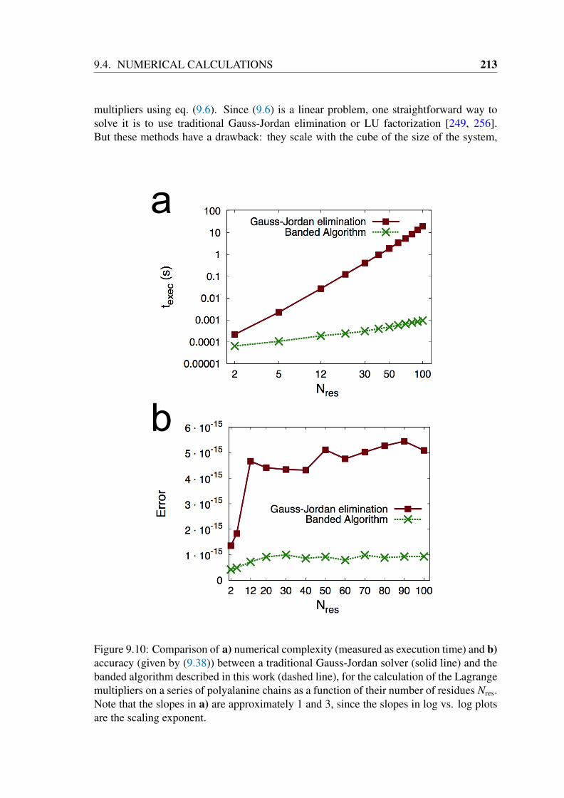
9.4. NUMERICAL CALCULATIONS 213
multipliers using eq. (9.6). Since (9.6) is a linear problem, one straightforward way tosolve it is to use traditional Gauss-Jordan elimination or LU factorization [249, 256].But these methods have a drawback: they scale with the cube of the size of the system,
a
b
Figure 9.10: Comparison of a) numerical complexity (measured as execution time) and b)accuracy (given by (9.38)) between a traditional Gauss-Jordan solver (solid line) and thebanded algorithm described in this work (dashed line), for the calculation of the Lagrangemultipliers on a series of polyalanine chains as a function of their number of residues Nres.Note that the slopes in a) are approximately 1 and 3, since the slopes in log vs. log plotsare the scaling exponent.

214 CHAPTER 9. LAGRANGE MULTIPLIERS IN BIOLOGICAL POLYMERS
Nres Gauss-Jordan Banded Alg. Gauss-Jordan Banded Alg.Error Error texec (s) texec (s)
2 1.355 · 10−15 4.193 · 10−16 2.185 · 10−4 6.500 · 10−5
5 1.829 · 10−15 4.897 · 10−16 2.263 · 10−3 1.059 · 10−4
12 4.660 · 10−15 7.244 · 10−16 2.733 · 10−2 1.897 · 10−4
20 4.413 · 10−15 9.160 · 10−16 0.1239 2.407 · 10−4
30 4.340 · 10−15 9.975 · 10−16 0.4075 3.115 · 10−4
40 4.318 · 10−15 8.591 · 10−16 0.9669 3.975 · 10−4
50 5.113 · 10−15 9.209 · 10−16 1.877 4.811 · 10−4
60 4.761 · 10−15 7.906 · 10−16 3.457 5.751 · 10−4
70 5.026 · 10−15 9.868 · 10−16 5.381 6.664 · 10−4
80 5.271 · 10−15 8.843 · 10−16 8.633 7.605 · 10−4
90 5.448 · 10−15 9.287 · 10−16 13.42 8.527 · 10−4
100 5.091 · 10−15 9.342 · 10−16 19.69 9.484 · 10−4
Table 9.1: Comparison of numerical complexity and accuracy between a traditionalGauss-Jordan solver and the banded algorithm described just before this, for the calcu-lation of the Lagrange multipliers on a series of polyalanine chains as a function of theirnumber of residues Nres.
i.e., if we imposed Nc constraints on our system (and therefore we needed to obtain Nc
Lagrange multipliers), the number of floating point operations that these methods wouldrequire is proportional to N3
c . However, as we showed in the previous sections, the factthat many biological molecules, and proteins in particular, are essentially linear, allowsthe constraints to be indexed in such a way that the matrix R in eq. (9.6) is banded, anddifferent techniques to be used for solving the problem which require only O(Nc) floatingpoint operations [1].
In fig. 9.10 and table 9.4, we compare both the execution time (a) and the accuracy (b)of the two different methods: Gauss-Jordan elimination [256], and the banded recursivesolution advocated here and made possible by the appropriate indexing of the constraints.The calculations have been run on a Mac OS X laptop with a 2.26 GHz Intel Core 2 Duoprocessor, and the errors were measured using the normalized deviation of Rλ from −o,i.e., if we denote by λ the solution provided by the numerical method,
Error :=
∑NcI=1
∣∣∣∑NcJ=1 RIJλJ + oI
∣∣∣∑NcI=1 |λI |
. (9.38)
From the obtained results, we can see that both methods produce an error which is verysmall (close to machine precision), being the accuracy of the banded algorithm advocatedin this work slightly higher. Regarding the computational cost, as expected, the Gauss-Jordan method presents an effort that approximately scales with the cube of the number ofconstraints Nc (which is approximately proportional to Nres), while the banded techniqueallowed by the particular structure of the matrix R follows a fairly accurate linear scaling.Although it is typical that, when two such different behaviours meet, there exists a rangeof system sizes for which the method that scales more rapidly is faster and then, at a givensystem size, a crossover takes place and the slower scaling method becomes more efficient

9.5. CONCLUSIONS 215
from there on, in this case, and according to the results obtained, the banded techniqueis less time-consuming for all the explored molecules, and the crossover should exist at avery small system size (if it exists at all). This is very relevant for any potential uses ofthe methods introduced in this work.
9.5 ConclusionsWe have shown that, if we are dealing with typical biological polymers, whose covalentconnectivity is that of essentially linear objects, the Lagrange multipliers that need to becomputed when Nc constraints are imposed on their internal degrees of freedom (such asbond lengths, bond angles, etc.) can be obtained in O(Nc) steps as long as the constraintsare indexed in a convenient way and banded algorithms are used to solve the associatedlinear system of equations. This path has been traditionally regarded as too costly inthe literature [237, 298, 393, 425–428], and, therefore, our showing that it can be im-plemented efficiently could have profound implications in the design of future MolecularDynamics algorithms.
Since it is well-known that the use of the exact Lagrange multipliers to solve the un-derlying ordinary differential equations produces unstable algorithms [237, 439], the fieldof imposition of constraints in Molecular Dynamics simulations is dominated by methodsthat ensure that the system stays exactly on the constrained subspace as the simulationproceeds, being some of the most popular approaches SHAKE [237], RATTLE [446] andLINCS [417]. The technique introduced in this work can be used to improve this type ofmethods:
• SHAKE and RATTLE consider a system of equations (σ = 0) which ensures thatconstraints are satisfied for every time step within a given tolerance. To this end,they iteratively solve an approximated linear problem. Although they do not ex-plicitly calculate the exact Lagrange multipliers, but approximations to them thatenforce the satisfaction of the constraints, the (non-symmetric) matrices appearingin both algorithms can be expressed as banded matrices if the constraints are clev-erly ordered (see supplementary material), and therefore they can be inverted witha banded algorithm like the one described here.
• LINCS does use the same equation (d2σdt2 = 0) as we do to calculate the Lagrange
multipliers, and then adds a correction term to ensure that the constraints are satis-fied in every time step. But instead of explicitly inverting R in (9.6), LINCS con-siders B := I − R (being I the identity matrix), and then approximates (I − B)−1 '
I+B+B2+B3+B4. This assumption is very efficient, but is only valid when the abso-lute value of all eigenvalues of B is less than 1, what in practice precludes the impo-sition of constraints on bond angles [417]. Our banded method can efficiently solvethe system without having this drawback, thus allowing to be inserted into LINCSto constrain bond angles. We call this method ILVES (Finnish word for “lynx”).The number of floating point operations required by ILVES and LINCS (taken asan estimation of their numerical complexities) is similar for the step of solving thelinear system, as it can be seen in fig. 9.11. We calculated the number of floatingpoint operations as follows. For ILVES (as can be seen in [1], where the banded

216 CHAPTER 9. LAGRANGE MULTIPLIERS IN BIOLOGICAL POLYMERS
Figure 9.11: Comparison of the efficiencies to solve the linear sparse system (8.1). Itis expressed as the quotient of the number of floating point operations of the bandedalgorithm (ILVES, based on (9.20)) divided by that of the approximation (I − B)−1 '
I + B + B2 + B3 + B4 (LINCS) as a function of the semi-band width m of the sparse bandedmatrix B.
operations are described), getting the diagonal ξ’s in (9.20) takes about 2mNc float-ing point operations, being m the semi-band width of the matrix R; calculating theξ’s above the diagonal takes about m2Nc floating point operations, and calculatingthose below the diagonal only mNc floating point operations using (9.21). Onceall ξ’s are known, solving the system takes about 8mNc floating point operations.Therefore, ILVES takes about (m2 + 11m)Nc floating point operations to solve thelinear banded system. If we use (I − B)−1 ' I + B + B2 + B3 + B4 being B a bandedmatrix with semi-band width m, we first have to build B from R, what takes Nc float-ing point operations. Then matrix-vector products are performed, each taking about(2m + 1)Nc products and 2mNc additions. Since it has to be done four times, and thecorresponding terms have to be added, the total number of floating point operationswill be about (16m + 9)Nc. The quotient between both numerical complexities in-creases as a function of m, but in the most interesting cases of biological polymers,m will not be very large, as we have shown in the previous sections. Notice that,in fig. 9.11, we are not comparing the total number of operations of ILVES andLINCS, but only the part of them in which R−1o is computed. Building the matrixR and the calculation of the subsequent correcting terms are common steps in bothalgorithms.
It is worth mentioning that the accuracy up to which constraints are satisfied dependson the method to implement them. SHAKE and RATTLE rely on an iterative procedure,which is repeated until every constraint is satisfied within a chosen arbitrary tolerance
9.5. CONCLUSIONS 217
[237, 447]. The accuracy of LINCS depends on the order used in the expansion (I−B)−1 '
I + B+ B2 + B3 + B4 + . . .. For MD calculations a fourth order in the expansion is normallyenough, while for Brownian dynamics (with longer time steps) an eighth order expansionmay be necessary [448]. In any case, higher accuracies require more time-consumingcalculations (this increase in the cost can be very high [449]). Therefore, an equilibriumbetween accuracy and numerical complexity has to be sought by an appropriate choice ofthe parameters present in any method (except for methods such as the one introduced here,which does not contain any parameter). To this end, prior to any simulation, some testshave to be performed. These tests (which can be run either on the system we are going tosimulate or on a toy one) must measure the accuracy of a series of observable quantity asa function of the parameter contained in the method (like TOL in Amber’s [254] SHAKE,shake_tol in Gromacs’ [114] SHAKE or lincs_order in Gromacs’ LINCS). With thisdata, together with the computational cost as a function of the same parameter, a practicaldecision must be taken based on available resources and desired accuracy.
It is clear from the presented examples that, in addition to its application to SHAKE,RATTLE and LINCS, the new techniques introduced here can be applied to many ofthe rest of approaches mentioned in sec. 9.1, as well as to the development of new suchtechniques.
Finally, we are exploring an extension of the ideas introduced here to the calculationnot only of the Lagrange multipliers but also of their time derivatives (see appendix D),to be used in higher order integrators than Verlet. Since the sparsity of the matrices tocalculate these derivatives is the same as that of the matrix R in this work, the samebanded techniques can be used to solve the problem.

Appendices
A Corrections for the Fast Multipole Method in a gridThe fast multipole method (FMM) [258, 450] was devised to efficiently calculate pairwisepotentials created by pointlike charges, like pairwise Coulomb potential. In the literatureit is possible to find some modifications of the traditional FMM which deal with chargeswhich are modelled as Gaussian functions. Such modifications of FMM can be used intoLCAO codes as Gaussian [162] or FHI-Aims [163]. However, they cannot be used whenthe charge distribution is represented through a set of discrete charge density values. TheFast Multipole Method presented in [184] belongs to the kind of pointlike charges FMM’s.The referred implementation is very accurate and efficient, but it requires some modifica-tions to work in programs like Octopus. Octopus [6, 171] is a code for ab initio quantumdensity functional theory calculations which operates with the electronic density (ρ) asvariable. This electronic density is a continuous variable, but is sampled in Octopus intodiscrete values (see chap. 4). The electronic density used by Octopus is an R3 → R field,where the values of the R3 set correspond to a equispaced mesh (see fig. A.1 c) ). Forexample, if the spacing in the x direction is L1, the spacing in the y direction is L2 andthe spacing in the z direction is L3, some points ~x of the mesh can be (−3L1,−3L2,−3L3),(−3L1,−3L2,−2L3), (−3L1,−3L2,−L3), . . ., (−2L1,−3L2,−3L3), . . ., (3L1, 3L2, 3L3). Usu-ally, L1 = L2 = L3 := L. The only constraints on the electronic density ρ(~x) are
• ρ(~x) is negative for all ~x
• ρ(~x) is expected to vary slowly among nearby ~x points
In Octopus, every value of ρ(~r0) represents the electronic density in a cubic cell ofvolume L1L2L3 centered in~r0. In the currently implemented version of FMM for Octopus,the total potential in ~x (i.e., V(~r0)) is calculated as the summation of FMM point pairwisecalculation plus a self interaction term for the cell centered in ~r0 itself. So
V(~r0) = VFMM(~r0)L3 + VS el f Int.(~r0) , (A.1)
being
VS el f Int.(~r0) =
∫Cell
d~xρ(~x)|~x − ~r0|
= ρ(~r0)∫
Celld~x
1|~x − ~r0|
' ρ(~r0)∫ R
0dr
∫ 2π
0dφ
∫ π
0dθ
r2sen(θ)r
= ρ(~r0)2πL2(
34π
)2/3
. (A.2)

220 APPENDICES
Figure A.1: Simple scheme to give a notion of the way to correct the integrals for theHartree potential. Green points indicate grid points. Magenta points are are auxiliarypoints which neighbour a given grid point (P).
In (A.3) we have not integrated over a cubic cell, but over a spherical cell whose volumeis the same as that of the original cubic cell (L3). This determines the value of R (L3 =
4/3πR3). Numerical integration of the cubic cell gives almost the same result. In (A.1) wecan notice a factor L3. It comes with the potential calculated by FMM because the inputoctopus provides FMM is a charge density, rather than a charge.
If Li for i = 1, 2, 3 are not equal, then
VS el f Int.(~r0) = ρ(~r0)2π(L1L2L3)2/3(
34π
)2/3
. (A.3)
The formula of (A.1) results in a global accuracy which we need to improve in orderto have reliable results for quantum systems. For these, charge distribution is expectedto be similar to sets of Gaussians centered in the atoms of the system. For Gaussiandistributions, the greatest concavity near the center of the Gaussian make (as far as weknow) the influence of neighbouring points to be major for V . As we can see in thescheme of fig. A.1 a)-b), considering semi-neighbours of point P (in~r0), i.e., points whosedistance to ~r0 is not L, but L/2, the integral of (A.1) can be calculated in a much more

A CORRECTIONS FOR THE FAST MULTIPOLE METHOD IN A GRID 221
accurate way. So, we would like to have an expression for V such as
V(~x) = VFMM(~x)L3 + VS el f Int.(~x) + VCorrect.(~x) , (A.4)
where VCorrect.(~x) is a function of the charge in the points neighbouring ~x. If Li vary,replace L3 above by L1L2L3
Method 1: 6-neighbours correctionWe build a corrective term by calculating the charg in the 6 semi-neighbours of everypoint of the mesh ~r0 (see fig. A.2 for a intuitive scheme). We use the formula por the 3rddegree interpolation polynomial:
f (0) =−116
f(−32
L)
+9
16f(−L2
)+
916
f(L
2
)+−116
f(32
L), (A.5a)
f(−L2
)=−116
f (−2L) +916
f (−L) +916
f (0) +−116
f (L) , (A.5b)
f(L
2
)=−116
f (−L) +9
16f (0) +
916
f (L) +−116
f (2L) . (A.5c)
So, the semi-neighbours of ~r0 = (x0, y0, z0) are
ρ(x0 − L/2, y0, z0) =−116ρ (x0 − 2L, y0, z0) +
916ρ (x0 − L, y0, z0) +
916ρ (x0, y0, z0) −
116ρ (x0 + L, y0, z0) ; (A.6a)
ρ(x0 + L/2, y0, z0) =−116ρ (x0 − L, y0, z0) +
916ρ (x0, y0, z0) +
916ρ (x0 + L, y0, z0) −
116ρ (x0 + 2L, y0, z0) ; (A.6b)
ρ(x0, y0 − L/2, z0) =−116ρ (x0, y0 − 2L, z0) +
916ρ (x0, y0 − L, z0) +
916ρ (x0, y0, z0) −
116ρ (x0, y0 + L, z0) ; (A.6c)
ρ(x0, y0 + L/2, z0) =−116ρ (x0, y0 − L, z0) +
916ρ (x0, y0, z0) +
916ρ (x0, y0 + L, z0) −
116ρ (x0, y0 + 2L, z0) ; (A.6d)
ρ(x0, y0, z0 − L/2) =−116ρ (x0, y0, z0 − 2L) +
916ρ (x0, y0, z0 − L) +
916ρ (x0, y0, z0) −
116ρ (x0, y0, z0 + L) ; (A.6e)
ρ(x0, y0, z0 + L/2) =−116ρ (x0, y0, z0 − L) +
916ρ (x0, y0, z0) +
916ρ (x0, y0, z0 + L) −
116ρ (x0, y0, z0 + 2L) . (A.6f)
We consider all this six charges to be homogeneously distributed in cells whose volume isL3/8. The distance between the center of these small cells and the center of the cell whoseV we are calculating (i.e., the cell centered in ~r0) is L/2. So the first part of VCorrect.(~r0) is

222 APPENDICES
VCorr.+ = (A.7)(L3
8
) (1
L/2
) [ρ(x0 − L/2, y0, z0) + ρ(x0 + L/2, y0, z0) + . . . + ρ(x0, y0, z0 + L/2)
].
Since we have created these new 6 cells, we must substract its corresponding volume fromthe cells whose space is occupied by these new cells. This amount is
VCorr.− = (ρ(x0 − L, y0, z0) + ρ(x0 + L, y0, z0) + ρ(x0, y0 − L, z0) + ρ(x0, y0 + L, z0)
+ ρ(x0, y0, z0 − L) + ρ(x0, y0, z0 + L))(
L3
16
) (1L
)+ αVS el f Int. . (A.8)
The parameter α is to be tuned, because the integral in (A.4) is not homogeneously dis-tributed, and therefore α does not need to be 6/(2 · 8). Our first stimation gave a valueα = 6/20.3 (this value minimized the errors in the potentials).
If L1 , L2 , L3
ρ(x0 − L1/2, y0, z0) =−116ρ (x0 − 2L1, y0, z0) +
916ρ (x0 − L1, y0, z0) +
916ρ (x0, y0, z0) −
116ρ (x0 + L1, y0, z0) ; (A.9a)
ρ(x0 + L1/2, y0, z0) =−116ρ (x0 − L1, y0, z0) +
916ρ (x0, y0, z0) +
916ρ (x0 + L1, y0, z0) −
116ρ (x0 + 2L1, y0, z0) ; (A.9b)
ρ(x0, y0 − L2/2, z0) =−116ρ (x0, y0 − 2L2, z0) +
916ρ (x0, y0 − L2, z0) +
916ρ (x0, y0, z0) −
116ρ (x0, y0 + L2, z0) ; (A.9c)
ρ(x0, y0 + L2/2, z0) =−116ρ (x0, y0 − L2, z0) +
916ρ (x0, y0, z0) +
916ρ (x0, y0 + L2, z0) −
116ρ (x0, y0 + 2L2, z0) ; (A.9d)
ρ(x0, y0, z0 − L3/2) =−116ρ (x0, y0, z0 − 2L3) +
916ρ (x0, y0, z0 − L3) +
916ρ (x0, y0, z0) −
116ρ (x0, y0, z0 + L3) ; (A.9e)
ρ(x0, y0, z0 + L3/2) =−116ρ (x0, y0, z0 − L3) +
916ρ (x0, y0, z0) +
916ρ (x0, y0, z0 + L3) −
116ρ (x0, y0, z0 + 2L3) . (A.9f)
We consider all this six charges to be homogeneously distributed in cells whose volume isL1L2L3/8. The distance between the center of these small cells and the center of the cellwhose V we are calculating (i.e., the cell centered in ~r0) is L1/2, L2/2 or L3/2. So the firstpart of VCorrect.(~r0) is
A CORRECTIONS FOR THE FAST MULTIPOLE METHOD IN A GRID 223
VCorr.+ =
(L1L2L3
8
) [(ρ(x0 − L1/2, y0, z0) + ρ(x0 + L1/2, y0, z0))
(1
L1/2
)+
(ρ(x0, y0 − L2/2, z0) + ρ(x0, y0 + L2/2, z0))(
1L2/2
)+
(ρ(x0, y0, z0 − L3/2) + ρ(x0, y0, z0 + L3/2))(
1L3/2
) ]. (A.10)
Since we have created these new 6 cells, we must substract its corresponding volume fromthe cells whose space is occupied by these new cells. This amount is
VCorr.− =
(L1L2L3
16
) [(ρ(x0 − L1, y0, z0) + ρ(x0 + L1, y0, z0))
(1L1
)+ ((ρ(x0, y0 − L2, z0) + ρ(x0, y0 + L2, z0))
(1L2
)(A.11)
+ ((ρ(x0, y0, z0 − L3) + ρ(x0, y0, z0 + L3))(
1L3
) ]+ αVS el f Int. .
Thus, VCorrect = VCorr.+ − VCorr.−, and we can build a correction for V(~r0) that is onlyfuncion of ρ(~r0) and of the charges neighbouring ~r0 (two first neighbours in all 3 cardinaldirections). In our tests, we used R :=
√∑i(VExact(~xi) − VFMM(~xi))2, index i running for
all points of the system. The inclusion of the correcting term introduced in this sectionreduced R in a factor about 50.
Method 2: 124-neighbours correction
This method is similar to the one explained in the previous section, but with two differ-ences
é It uses 3D interpolation polynomials, instead of 1D polynomials. Then, it considers53−1 = 124 neighbours in a cube of edge 5L centered in~r0 to calculate the correctiveterm for V(~r0)
é The interpolation polynomials representing ρ(x, y, z) are numerically integrated (af-ter their division by r). This is, we calculate
VCorr.+(~r0) =
∫Cell−125L3
d~xρ(~x)|~x − ~r0|
'
∫Cell−125L3
d~xPol(~x)|~x − ~r0|
. (A.12)
The integration is to be performed between -5/2L and 5/2L for x, y and z. The interpolationpolynomial (with 125 support points) Pol(~x) is
Pol(~x) =
5∑i=1
5∑j=1
5∑k=1
ρ(x0 + (i − 3)L, y0 + ( j − 3)L, z0 + (k − 3)L)αi(x)α j(y)αk(z) , (A.13)

224 APPENDICES
Figure A.2: 2D example of the position of cells containing semi neighbours. Assume thecenter of the plots is ~r0, the point where we want to calculate the correcting term for thepotential. The volume of semi-neighbour cells is L2/4 in 2D, and L3/8 in 3D. One half ofthe semi-neighbour cell occupies the voulume of a neighbour cell (the cell whose centeris L away from ~r0). The other half of the semi-neighbour cell occupies the space of the~r0-centered cell itself.
being
α1(ξ) :=ξ4
24−ξ3
12−ξ2
24+ξ
12, (A.14a)
α2(ξ) := −ξ4
6+ξ3
6+
2ξ2
3−
2ξ3, (A.14b)
α3(ξ) :=ξ4
4−
5ξ2
4+ 1 , (A.14c)
α4(ξ) := −ξ4
6−ξ3
6+
2ξ2
3+
2ξ3, (A.14d)
α5(ξ) :=ξ4
24+ξ3
12−ξ2
24−ξ
12. (A.14e)
The quotient of the polynomials αi(x)α j(y)αk(z) divided by |~x − ~r0| can be numericallyintegrated through the cubic cell of edge 5L and centered in x0. Such integrals can indeed

A CORRECTIONS FOR THE FAST MULTIPOLE METHOD IN A GRID 225
be tabulated, because equation (A.12) implies VCorr.+(~r0) = VCorr.+(~r0)|L=1 · L2. Termsof αi(x)α j(y)αk(z)/|~x − ~r0| are often odd functions whose integral is null. The non-zerointegrals taking part in (A.3) with L = 1 are displayed below.∫ 1/2
−1/2dx
∫ 1/2
−1/2dy
∫ 1/2
−1/2dz
x0y0z0
|~x − ~r0|= 2.38008 , (A.15a)∫
x2y0z0
|~x − ~r0|=
∫x0y2z0
|~x − ~r0|=
∫x0y0z2
|~x − ~r0|= 0.160099 , (A.15b)∫
x4y0z0
|~x − ~r0|=
∫x0y4z0
|~x − ~r0|=
∫x0y0z4
|~x − ~r0|= 0.0224242 , (A.15c)∫
x2y2z0
|~x − ~r0|=
∫x2y0z2
|~x − ~r0|=
∫x0y2z2
|~x − ~r0|= 0.0117336 , (A.15d)∫ 1/2
−1/2dx
∫ 1/2
−1/2dy
∫ 1/2
−1/2dz
x2y2z2
|~x − ~r0|= 0.000888104 , (A.15e)∫
x0y2z4
|~x − ~r0|=
∫x0y4z2
|~x − ~r0|=
∫x2y0z4
|~x − ~r0|= 0.00167742 , (A.15f)∫
x2y4z0
|~x − ~r0|=
∫x4y0z2
|~x − ~r0|=
∫x4y4z0
|~x − ~r0|= 0.00167742 , (A.15g)∫
x1y4z4
|~x − ~r0|=
∫x4y1z4
|~x − ~r0|=
∫x4y4z1
|~x − ~r0|= 0.000241275 , (A.15h)∫
x4y2z2
|~x − ~r0|=
∫x2y4z2
|~x − ~r0|=
∫x2y2z4
|~x − ~r0|= 0.000128276 , (A.15i)∫
x4y4z2
|~x − ~r0|=
∫x2y4z4
|~x − ~r0|=
∫x4y2z4
|~x − ~r0|= 0.0000185935 , (A.15j)∫ 1/2
−1/2dx
∫ 1/2
−1/2dy
∫ 1/2
−1/2dz
x4y4z4
|~x − ~r0|= 0.00000270259 . (A.15k)
Therefore
VCorr.+(~r0) =
5∑i=1
5∑j=1
5∑k=1
ρ(x0 + (i − 3)L, y0 + ( j − 3)L, z0 + (k − 3)L) ·∫Cell−125L3
d~xαi(x)α j(y)αk(z)|~x − ~r0|
=
5∑i=1
5∑j=1
5∑k=1
ρ(x0 + (i − 3)L, y0 + ( j − 3)L, z0 + (k − 3)L) ·
5∑l=1
5∑m=1
5∑n=1
αi,lα j,mαk,n
∫Cell−125L3
d~xxl−1ym−1zn−1
|~x − ~r0|
=
5∑i=1
5∑j=1
5∑k=1
ρ(x0 + (i − 3)L, y0 + ( j − 3)L, z0 + (k − 3)L) ·
5∑l=1
5∑m=1
5∑n=1
αi,lα j,mαk,nβ(l − 1,m − 1, n − 1)L2 , (A.16)

226 APPENDICES
where αi,l is the coefficient of ξl−1 if αi(ξ) and
β(l,m, n) :=∫ 1/2
−1/2dx
∫ 1/2
−1/2dy
∫ 1/2
−1/2dz
xlymzn√x2 + y2 + z2
. (A.17)
In this case, VCorr.− is equal to all the contributions to V(~r0) due to charges whose position(x, y, z) satisfies
|x − x0| <= 2L; |y − y0| <= 2L; |z − z0| <= 2L , (A.18)
including self-interaction integral.This way to calculate VCorr.+ is not inefficient, because only 27 integrals are not null,
and both α and β are known. In order to calculate VCorr.+(~r0) we need 125 products andadditions, what is essentially the same number of operations which is required in order tocalculate the potential created in ~r0 by the neighbouring points (whose calculation can beremoved and then saved). Surprisingly, results using this correction method were worsethan that obtained using the first method.

B SUPPLEMENTARY INFORMATION FOR CHAPTER 5 227
B Supplementary information for chapter 5
Basis Set ConvergenceTable B.2 shows the convergence of the CC2 excitation energy for the anionic and neutralHBDI chromophore in vacuo. Diffuse augmentation is required for gas-phase calcula-tions. An even faster convergence is expected in the condensed phase. The aug-SV(P)basis produces converged results and is used throughout the paper for CC2 and SORCIcalculations.
basis set anionic neutralSV(P) 3.07 3.91cc-pVDZ 3.04 3.84aug-SV(P) 2.88 3.72aug-cc-pVDZ 2.88 3.69aug-cc-pVTZ 2.87 3.68
Table B.2: CC2 S1 Excitation Energies (eV) of HBDI in Vacuo. The B3LYP/TZVP ge-ometry has been used in all cases.
Generalized Bond Length AlternationWe define a generalized bond length alternation (GBLA) by projecting the cartesian gra-dient G of the excitation energy onto bonds
GBLA =∑
i ζi|RA − RB| ; ζi =
∑i(RA − RB) · (GA −GB)
|(RA − RB|, (B.1)
where i runs over all bonds within the π-system of HBDI. Adopting the bond numberingof Laino et al. [226], the normalized coefficients ζi obtained from an CC2/aug-SV(P)gradient calculation of the S1 ←S0 excitation energy are given in Table B.3. The onlyarbitrariness consists in the choice of the reference geometry, which we choose to be theCC2/aug-SV(P) ground state minimum. Values for the planar excited state minimum areshown for comparison.
bond 1 2 3 4 5 6 7 8anionic -0.0172 -0.0097 -0.0142 -0.0494 0.0329 -0.0359 0.0088 0.0165neutral -0.0564 0.0649 -0.1137 0.0853 0.0775 -0.0885 0.0458 -0.0204bond 9 10 11 12 13 14 15anionic 0.0183 -0.0195 0.0093 0.0278 -0.0274 0.0239 -0.0319neutral -0.0359 0.0263 -0.0205 -0.0041 0.0121 -0.0368 0.0117
Table B.3: CC2/def2-TZVP Gradient of the HBDI S1 ←S0 Excitation Energy Projectedonto Bonds.. Bonds are numbered following Ref [226].

228 APPENDICES
TDDFT Time-Propagation Spectra
0
1
2
3
4
5
1.5 2 2.5 3 3.5 4
Abs
orpt
ion
(a.u
.)
Energy (eV)
Neutral A, gga pbe, t=60
CT-------------------------------(n+π)→π*-----[ CT ]+[ π → π* ] -------------------
π → π*[ π → π* ] + [ CT ]
π → π*π → π*36 atom, w/o p. ch.
36 atom with p. ch.73 atom, w/o p. ch.73 atom, with p. ch.
0
1
2
3
4
5
1.5 2 2.5 3 3.5 4
Abs
orpt
ion
(a.u
.)Energy (eV)
Anionic B, gga pbe, t=30
π → n+π*
[ π → π* ] + [ CT ]---- [ CT ] + [ π → π* ]
π → π*π → π*
π → π*
35 atom, w/o p. ch.35 atom with p. ch.73 atom, w/o p. ch.73 atom, with p. ch.
0
1
2
3
4
5
1.5 2 2.5 3 3.5 4
Abs
orpt
ion
(a.u
.)
Energy (eV)
Neutral A, gga blyp, t=60
[ CT ] + [ π → π* ] --------------------CT ------------ --------------- CT
(n+π)→π*---------------
[ π → π* ] + [ CT ] ------------------π → π*--- π → π*
π → π*36 atom, w/o p. ch.36 atom with p. ch.73 atom, w/o p. ch.73 atom, with p. ch.
0
1
2
3
4
5
1.5 2 2.5 3 3.5 4
Abs
orpt
ion
(a.u
.)
Energy (eV)
Anionic B, gga blyp, t=30
[ CT ] + [ π → π* ]
--- [ CT ] + [ π → π* ]
π → π*
π → n+π*
π → π*
π → π*
35 atom, w/o p. ch.35 atom with p. ch.73 atom, w/o p. ch.73 atom, with p. ch.
0
1
2
3
4
5
1.5 2 2.5 3 3.5 4
Abs
orpt
ion
(a.u
.)
Energy (eV)
Neutral A, lda vwn, t=60
CT-------------------------------- -------------- CT (n+π)→π*------------CT ------
π → π*----------------------π → π*
π → π*π → π*36 atom, w/o p. ch.36 atom with p. ch.73 atom, w/o p. ch.73 atom, with p. ch.
0
1
2
3
4
5
1.5 2 2.5 3 3.5 4
Abs
orpt
ion
(a.u
.)
Energy (eV)
Anionic B, lda vwn, t=30
π → n+π*
[ π → π* ] + [ CT ] --- [ CT ] + [ π → π* ]
π → π*π → π*
π → π*
35 atom, w/o p. ch.35 atom with p. ch.73 atom, w/o p. ch.73 atom, with p. ch.
Figure B.1: TDDFT time-propagation spectra of GFP in A and B form for differentGGA/LDA functionals. Results with QM1 (36 atoms) and QM2 (73 atoms) regions arepresented.
Figure B.1 shows the simulated absorption spectra from TDDFT time propagation.The band were assigned by comparison with linear-response LCAO calculations.
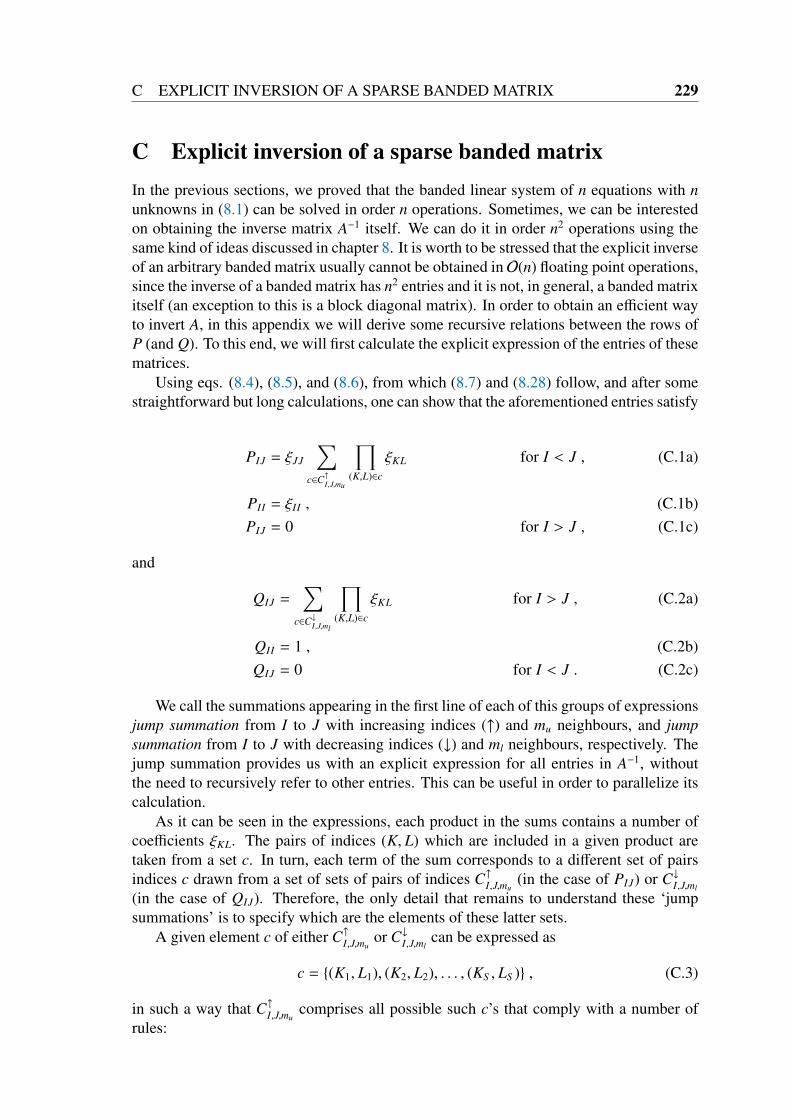
C EXPLICIT INVERSION OF A SPARSE BANDED MATRIX 229
C Explicit inversion of a sparse banded matrixIn the previous sections, we proved that the banded linear system of n equations with nunknowns in (8.1) can be solved in order n operations. Sometimes, we can be interestedon obtaining the inverse matrix A−1 itself. We can do it in order n2 operations using thesame kind of ideas discussed in chapter 8. It is worth to be stressed that the explicit inverseof an arbitrary banded matrix usually cannot be obtained in O(n) floating point operations,since the inverse of a banded matrix has n2 entries and it is not, in general, a banded matrixitself (an exception to this is a block diagonal matrix). In order to obtain an efficient wayto invert A, in this appendix we will derive some recursive relations between the rows ofP (and Q). To this end, we will first calculate the explicit expression of the entries of thesematrices.
Using eqs. (8.4), (8.5), and (8.6), from which (8.7) and (8.28) follow, and after somestraightforward but long calculations, one can show that the aforementioned entries satisfy
PIJ = ξJJ
∑c∈C↑I,J,mu
∏(K,L)∈c
ξKL for I < J , (C.1a)
PII = ξII , (C.1b)PIJ = 0 for I > J , (C.1c)
and
QIJ =∑
c∈C↓I,J,ml
∏(K,L)∈c
ξKL for I > J , (C.2a)
QII = 1 , (C.2b)QIJ = 0 for I < J . (C.2c)
We call the summations appearing in the first line of each of this groups of expressionsjump summation from I to J with increasing indices (↑) and mu neighbours, and jumpsummation from I to J with decreasing indices (↓) and ml neighbours, respectively. Thejump summation provides us with an explicit expression for all entries in A−1, withoutthe need to recursively refer to other entries. This can be useful in order to parallelize itscalculation.
As it can be seen in the expressions, each product in the sums contains a number ofcoefficients ξKL. The pairs of indices (K, L) which are included in a given product aretaken from a set c. In turn, each term of the sum corresponds to a different set of pairsindices c drawn from a set of sets of pairs of indices C↑I,J,mu
(in the case of PIJ) or C↓I,J,ml
(in the case of QIJ). Therefore, the only detail that remains to understand these ‘jumpsummations’ is to specify which are the elements of these latter sets.
A given element c of either C↑I,J,muor C↓I,J,ml
can be expressed as
c = (K1, L1), (K2, L2), . . . , (KS , LS ) , (C.3)
in such a way that C↑I,J,mucomprises all possible such c’s that comply with a number of
rules:

230 APPENDICES
• K1 = I, and LS = J.
• Kr < Lr, for r = 1, . . . , S .
• Kr+1 = Lr, for r = 1, . . . , S .
• Lr − Kr ≤ mu, for r = 1, . . . , S .
Let us see an example:∑c∈C↑3,6,2
∏(K,L)∈c
ξKL = ξ3,4ξ4,5ξ5,6 + ξ3,4ξ4,6 + ξ3,5ξ5,6 . (C.4)
The rules to determine the elements of C↓I,J,mlare analogous to the ones above but
taking into account that the indices decrease:
• K1 = I, and LS = J.
• Kr > Lr, for r = 1, . . . , S .
• Kr+1 = Lr, for r = 1, . . . , S .
• Kr − Lr ≤ ml, for r = 1, . . . , S .
An example would be:∑c∈C↓5,1,3
∏(K,L)∈c
ξKL = ξ5,4ξ4,3ξ3,2ξ2,1 + ξ5,3ξ3,2ξ2,1 + ξ5,4ξ4,2ξ2,1
+ ξ5,4ξ4,3ξ3,1 + ξ5,3ξ3,1 + ξ5,2ξ2,1 + ξ5,4ξ4,1 . (C.5)
If we first focus on P, it is easy to see that, according to the properties of the jumpsummation, we have∑
c∈C↑I,J,mu
∏(K,L)∈c
ξKL = ξI,I+1
∑c∈C↑I+1,J,mu
∏(K,L)∈c
ξKL
+ ξI,I+2
∑c∈C↑I+2,J,mu
∏(K,L)∈c
ξKL
+ . . . + ξI,I+mu
∑c∈C↑I+mu ,J,mu
∏(K,L)∈c
ξKL . (C.6)
If we insert a multiplicative factor ξJJ at both sides and use (C.1), this equation be-comes eq. (8.32) obtained in sec. 8.2:
PIJ =
minI+mu,n∑K=I+1
ξIKPKJ for I < J .
An analogous expression for Q can be obtained in a similar way:
QIJ =
minJ+ml,n∑L=J+1
QILξLJ for I > J .

C EXPLICIT INVERSION OF A SPARSE BANDED MATRIX 231
Now, if we define µ1 := minmu, J − I, and µ2 := minml, I − J, since A−1 = PQ (see(8.3)), we have that
(A−1)IJ = (PQ)IJ =
n∑K=1
PIKQKJ =
n∑K=J
PIKQKJ =
=
n∑K=J
I+µ1∑L=I+1
PLKξIL
QKJ =
I+µ1∑L=I+1
ξIL
n∑K=J
PLKQKJ
=
I+µ1∑L=I+1
ξIL(A−1)LJ for I < J , (C.7)
which is a recursive relationship for the superdiagonal entries of A−1.Peforming similar computations, we have
(A−1)II = ξII +
I+µ1∑L=I+1
ξIL(A−1)LJ = ξII +
J+µ2∑L=J+1
ξLJ(A−1)IL , (C.8)
(A−1)IJ =
J+µ2∑L=J+1
ξLJ(A−1)IL for I > J . (C.9)
Using the last three equations, we can easily construct an algorithm to compute A−1 inO(n2) floating point operations. This algorithm would first calculate (A−1)nn = ξnn. Thenit would use (C.7) to obtain, in this order, (A−1)n−1,n, (A−1)n−2,n, . . ., (A−1)1n. These are thesuperdiagonal (I < J) entries of the n-th column. Then, it would use (C.9) to obtain, inthis order, (A−1)n,n−1, (A−1)n,n−2, . . ., (A−1)n1, i.e., the subdiagonal (I > J) entries of then-th row. Once the n row and column of A−1 are known, (A−1)n−1,n−1 can be obtained with(C.8), and then (C.7) and (C.9) can be used to obtain the entries of this (n − 1) columnand row, respectively. When calculating the entries of a column J, i.e., ξKJ with K < J,ξLJ is to be obtained always before ξL−1,J. When calculating the entries of a row I, i.e.,ξIK with I > K, ξIK is to be obtained always before ξI,K−1. This procedure can be repeatedfor all rows and columns of A−1, and the calculation of the K-th row and column can beperformed in parallel.

232 APPENDICES
D Efficient calculation of derivatives of Lagrange multi-pliers into Robotics
IntroductionIn this Ph. D. dissertation, statements about efficient construction of a linear system forthe calculation of Lagrange multipliers and the efficient solution of it were presented inchapters 8 and 9. The schemes of these chapters can be applied to calculate the constraintforces in robot arms and parallel manipulators as the ones displayed in fig. D.1.
Motion of mechanic articulated systems can be described by using adapted coordi-nates subject to holonomic non-flexible constraints (i. e., whose expression f (x, a) = 0being x positions in the system and a constant parameters). Computer simulation of themotion of such systems requires the evaluation of the forces acting on them, and amongthese are those forces arising from the imposition of constraints (constraint forces). Ei-ther the system trajectories are to be calculated with a more and more accuracy, or thesimulation time step is to be increased, integrators of increasing order are to be chosen,what will require the evaluation of the derivatives of the constraint forces. Frequently, thegeometry of articulated systems is essentially linear (e.g. arm-shaped, like a robot arm,or branched-trunk-shaped, like a parallel manipulator). For a system with Nc constraints,such geometry permits to calculate the constraint forces acting on it and their derivativesin order Nc operations, instead of the common order N3
c operations. This can be doneexactly (up to machine precision), without any iterative procedure involved. In this re-port we present the essentials of the mathematics that could be used to efficiently solvea rototic articulated system (hexapod parallel manipulator). It is devised as the first stepfor its computer implementation, which must be obtained after a brief algebra and theapplication of standard calculation routines.
Analysing a hexapod-shaped parallel manipulatorThis section is an attempt to improve the efficiency of the dynamics simulation of a typicalparallel manipulator. More efficiency in real-time simulations as the one presented in[451] is expected to enable the use of higher order integrators (see the next section) thusallowing also higher accuracy for the simulated quantities.
The hexapod we are going to analyse is the one displayed in fig. D.2. It is formed bysix legs, an upper plate and a lower plate fixed to the floor. Each leg is formed by twocoaxial cylinders, the upper terminal of the upper one being jointed to the upper plate bya spherical articulation, and the lower terminal of the lower one being jointed to the lowerplate by another spherical articulation. All twelve cylinders and the upper plate are treatedas rigid solids. Since every rigid solid has six degrees of freedom (DOF’s), our hexapodhas N := 78 DOFs’ (which will be reduced after the imposition of constraints).
We will describe the motion of every rigid solid by using adapted coordinates, whichare the position of its mass center and the three Euler angles giving its orientation in theZXZ convention (of course, any other could be used, but this one is expected to havegreater efficiency) The use of internal coordinates (i.e., bond lengths, bond angles anddihedral angles between different parts of our system) may slow the calculations downwhen calculating different quantities (since many transformations could be required) and

D EFFICIENT CALCULATION OF DERIVATIVES OF LAGRANGEMULTIPLIERS INTO ROBOTICS 233
Figure D.1: Top: Picture of a standard robot arm. Bottom: Scheme of a parallel manipu-lator. Courtesy of M. Díez.
may also lead to instabilities during the simulation [452]. The only external forces actingon our parallel manipulator are the gravity and the motor force, which is exerted withinevery hexapod leg. Gravity is only acting on mass center coordinates (we consider ~gconstant, thus not genetating any torque). The motor forces are assumed to be known. Weconsider they move the center of mass of the upper cylinder of every leg in the directionof its axis without any friction. This implies they are neither generating any torque. Inaddition to these external forces, the articulations between the different rigid solids areexerting contact constraint forces. We will assume the D’Alembert principle (i.e., we willconsider the constraint forces are not doing any work).
In this section we will use the following notation
• α , β = 1, . . . , 13 for rigid solids
• µ , ν = 1, . . . , 78 for coordinates of rigid solids

234 APPENDICES
Figure D.2: Top: Scheme of the analysed hexapod-shaped parallel manipulator. Courtesyof M. Díez and A. Zubizarreta.
• I, J = 1, . . . , 48 for constrains and for rows and columns of matrices
• i = 1, . . . , 6 for legs of the hexapod
• j = 1, 3, 5, 7, 9, 11 for lower cylinders
• k = 2, 4, 6, 8, 10, 12 for upper cylinders
We are going to calculate the constraints using eq. (9.3), which requires to knowthe second temporal derivatives of all coordinates. We will find them using the Euler-Lagrange equations. Equations presented in the previous section are valid for Cartesian

D EFFICIENT CALCULATION OF DERIVATIVES OF LAGRANGEMULTIPLIERS INTO ROBOTICS 235
coordinates. This is, expressions (9.1a), (9.3) and (9.4) are valid whenever the involvedcoordinates (xµ) are coordinates of mass center positions. When other than strictly Carte-sian coordinates are used, the Euler-Lagrange equations are no longer (9.1a), but [453]
ddt
[∂T∂qµ
]−∂T∂qµ
= Fµ(q(t)) +
Nc∑I=1
λI∂σI
∂qµ(q(t)), µ = 1, . . . ,N, (D.1)
where T stands for the kinetic energy, Fµ stands for the external "force" acting on thecoordinate, and the rest of the right hand side correspond to the total constraint "force" onit. These terms are not actually forces, but rather generalized momenta (the inclusion ofEuler angles will make the derivatives of T with respect to them not to have dimensionsof force). In the general case, Fµ =
∑ξ( ~Fext)ξd~xξ/dqµ with ξ sweeping all the differentials
of volume of the body. However, in our case, we won’t have to perform calculations likethese, since no net external "force" is acting on the Euler angles, and if qµ is a Cartesiancoordinate (as is the case for centers of mass), Fµ has dimensions of force.
In the adapted coordinates we are using, the kinetic energy T of a rigid body is
T = TCM + T ∗ , (D.2a)
TCM =M2~x 2
CM , (D.2b)
T ∗ =12ωT Iω , (D.2c)
where M is the mass of the rigid body, ~xCM is the position of its center of mass, ω is itsangular velocity and I its inertia tensor.
The angular velocity as a function of the Euler angles [453] is
ω1
ω2
ω3
=
sin(θ)sin(ψ) cos(ψ) 0sin(θ)cos(ψ) −sin(ψ) 0
cos(θ) 0 1
φθψ
. (D.3)
The inertia tensors of the lower cylinders, upper cylinders and upper plate are, respec-tively
Ilc =
I1l 0 00 I1l 00 0 I2l
; Iuc =
I1u 0 00 I1u 00 0 I2u
; Iup =
Iu 0 00 Iv 00 0 Iw
. (D.4)
Equations (D.2c), (D.3) and (D.4) make that the angular components of the kinetic energy

236 APPENDICES
for the lower cylinders (lc), upper cylinders (uc) and upper plate (up) are
T ∗lc =12
(I1lsin2(θ j) + I2lcos2(θ j))φ j2
+ I2lcos(θ j)φ jψ j +I1l
2θ j
2+
I2l
2ψ j
2
for j = 1, 3, . . . , 11 , (D.5a)
T ∗uc =12
(I1usin2(θk) + I2ucos2(θk))φk2
+ I2ucos(θk)φkψk +I1u
2θk
2+
I2u
2ψk
2
for k = 2, 4, . . . , 12 , (D.5b)
T ∗up =Iu
2(sin2(θ13)sin2(ψ13)φ2
13 + cos2(ψ13)θ213 + 2sin(θ13)sin(ψ13)cos(ψ13)φ13 ˙θ13)+
Iv
2(sin2(θ13)cos2(ψ13)φ2
13 + sin2(ψ13)θ213 − 2sin(θ13)sin(ψ13)cos(ψ13)φ13 ˙θ13)+
Iw
2(cos2(θ13)φ2
13 + ψ213 + 2cos(θ13)φ13ψ13) . (D.5c)
These expressions for the kinetic energy make the left hand side of (D.1) be
qi = φ j → (I1l − I2l)2cos(θ j)sin(θ j)φ jθ j
+ (I1l + I2l)φ j + I2lcos(θ j)ψ j − I2lsin(θ j)ψ jθ j (D.6a)
qi = θ j → I1lθ j + (I2l − I1l)cos(θ j)sin(θ j)φ2 + I2lsin(θ j)φ jψ j (D.6b)qi = ψ j → I2lcos(θ j)φ j − I2l(sin(θ j)φ jθ j + I2lψ j , (D.6c)
qi = φk → (I1u − I2u)2cos(θk)sin(θk)φkθk
+ (I1u + I2u)φk + I2ucos(θk)ψk − I2usin(θk)ψkθk (D.6d)
qi = θk → I1uθk + (I2u − I1u)cos(θk)sin(θk)φ2 + I2usin(θk)φkψk (D.6e)qi = ψk → I2ucos(θk)φk − I2u(sin(θk)φkθk + I2uψk , (D.6f)
qi = φ13 → φ13(Iusin2(θ13)sin2(ψ13) + Ivsin2(θ13)cos2(ψ13) + Iwcos2(θ13))+ θ13(Iu − Iv)sin(θ13)sin(ψ13)cos(ψ13) + ψ13(Iw)cos(θ13)
+ θ213(Iu − Iv)cos(θ13)sin(ψ13)cos(ψ13)
+ φ13θ13(Iusin2(θ13) + Ivcos2(θ13) − Iw)2sin(θ13)cos(θ13)
+ φ13ψ13(Iu − Iv)2sin2(θ13)sin(ψ13)cos(ψ13)
+ θ13ψ13
((−Iu − Iv)sin(θ13)sin2(ψ13)
− Ivsin(θ13)cos2(ψ13) − Iwsin(θ13)), (D.6g)
qi = θ13 → φ13(Iu − Iv)sin(θ13)sin(ψ13)cos(ψ13)
+ θ13(Iucos2(ψ13) + Ivsin2(ψ13)
+ φ213(−Iusin2(ψ13) − Ivcos2(ψ13) + Iw)
+ φ13ψ13sin(θ13)((Iu − Iv)(cos2(ψ13) − sin2(ψ13)) + Iw)+ θ13ψ13(−Iu + Iv)2sin(ψ13))cos(ψ13) , (D.6h)
qi = ψ13 → φ13Iwcos(θ13) + ψ13Iw
+ φ13θ13sin(θ13)((Iv − Iu)(cos2(ψ13) − sin2(ψ13)) − Iw
)
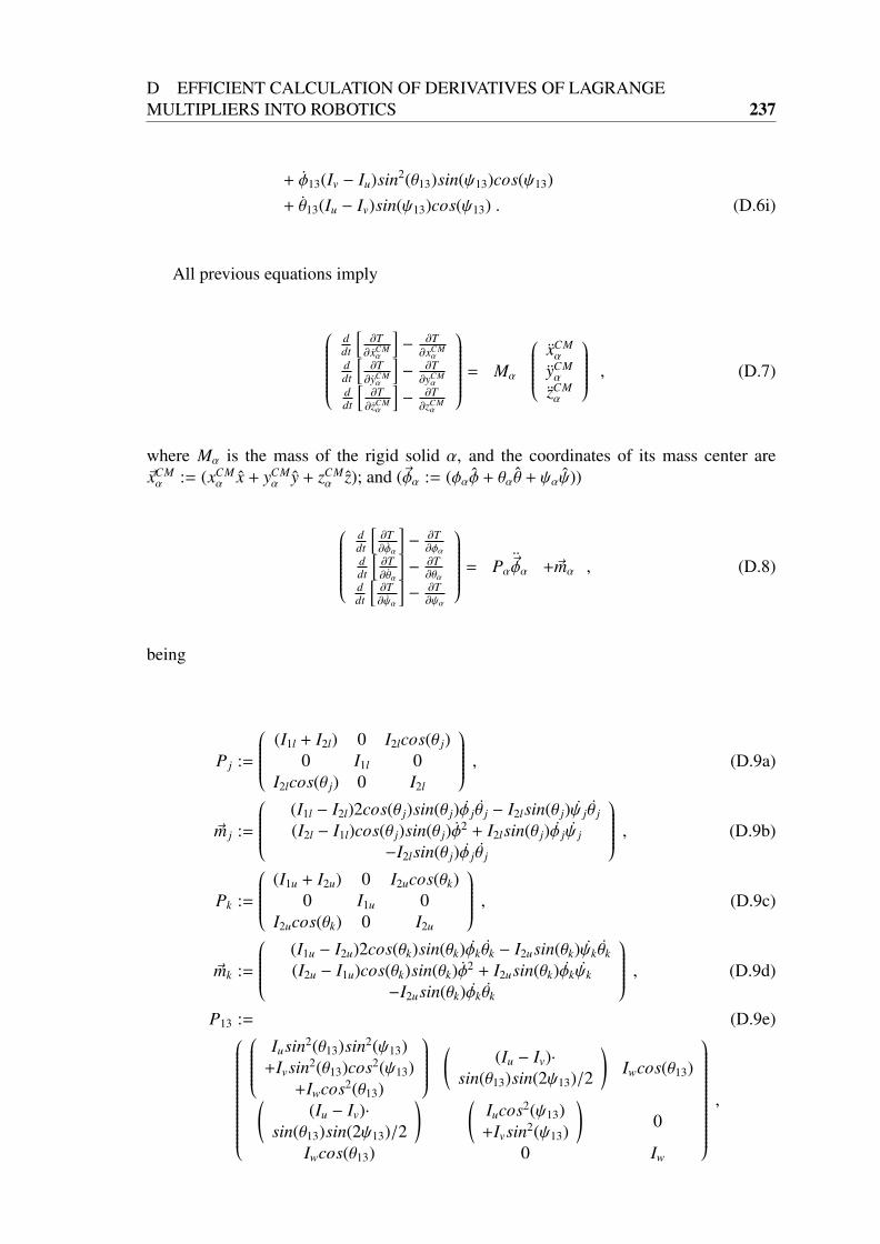
D EFFICIENT CALCULATION OF DERIVATIVES OF LAGRANGEMULTIPLIERS INTO ROBOTICS 237
+ φ13(Iv − Iu)sin2(θ13)sin(ψ13)cos(ψ13)+ θ13(Iu − Iv)sin(ψ13)cos(ψ13) . (D.6i)
All previous equations imply
ddt
[∂T∂xCM
α
]− ∂T
∂xCMα
ddt
[∂T∂yCM
α
]− ∂T
∂yCMα
ddt
[∂T∂zCMα
]− ∂T
∂zCMα
= Mα
xCMα
yCMα
zCMα
, (D.7)
where Mα is the mass of the rigid solid α, and the coordinates of its mass center are~xCMα := (xCM
α x + yCMα y + zCM
α z); and (~φα := (φαφ + θαθ + ψαψ))
ddt
[∂T∂φα
]− ∂T
∂φαddt
[∂T∂θα
]− ∂T
∂θαddt
[∂T∂ψα
]− ∂T
∂ψα
= Pα~φα +~mα , (D.8)
being
P j :=
(I1l + I2l) 0 I2lcos(θ j)0 I1l 0
I2lcos(θ j) 0 I2l
, (D.9a)
~m j :=
(I1l − I2l)2cos(θ j)sin(θ j)φ jθ j − I2lsin(θ j)ψ jθ j
(I2l − I1l)cos(θ j)sin(θ j)φ2 + I2lsin(θ j)φ jψ j
−I2lsin(θ j)φ jθ j
, (D.9b)
Pk :=
(I1u + I2u) 0 I2ucos(θk)0 I1u 0
I2ucos(θk) 0 I2u
, (D.9c)
~mk :=
(I1u − I2u)2cos(θk)sin(θk)φkθk − I2usin(θk)ψkθk
(I2u − I1u)cos(θk)sin(θk)φ2 + I2usin(θk)φkψk
−I2usin(θk)φkθk
, (D.9d)
P13 := (D.9e)
Iusin2(θ13)sin2(ψ13)+Ivsin2(θ13)cos2(ψ13)
+Iwcos2(θ13)
(
(Iu − Iv)·sin(θ13)sin(2ψ13)/2
)Iwcos(θ13)(
(Iu − Iv)·sin(θ13)sin(2ψ13)/2
) (Iucos2(ψ13)+Ivsin2(ψ13)
)0
Iwcos(θ13) 0 Iw
,

238 APPENDICES
~m13 :=
θ213(Iu − Iv)cos(θ13)sin(2ψ13)/2
+φ13θ13(Iusin2(θ13) + Ivcos2(θ13) − Iw)sin(2θ13)+φ13ψ13(Iu − Iv)2sin2(θ13)sin(2ψ13)/2+θ13ψ13
((−Iu − Iv)sin(θ13)sin2(ψ13)
−Ivsin(θ13)cos2(ψ13) − Iwsin(θ13))
+φ213(−Iusin2(ψ13) − Ivcos2(ψ13) + Iw)
+φ13ψ13sin(θ13)((Iu − Iv)(cos(2ψ13) + Iw)+θ13ψ13(−Iu + Iv)sin(2ψ13)) ,
φ13θ13sin(θ13)((Iv − Iu)(cos(2ψ13) − Iw)+φ13(Iv − Iu)sin2(θ13)sin(2ψ13)/2
+θ13(Iu − Iv)sin(2ψ13)/2 .
. (D.9f)
Shall we define
P :=
M1I3P1
M2I3P2
. . .
M13I3P13
;
~m :=
~g~m1
~FMotor2 /M2 + ~g
~m2...~g~m13
; ~u :=
~xCM1~φ1
~xCM2~φ2...
~xCM13~φ13
(D.10)
where ~g is the acceleration of the gravity, I3 is the identity matrix of rank 3 and Mα is themass of the respective rigid solid. The inverse of P is a block diagonal matrix
P−1 :=
1M1I3
P−11
1M2I3
P−12
. . .1
M13I3
P−113
(D.11)
It is to be stressed that the sparsity is essentially kept when inverting Pα. If α = 1, . . . , 12,

D EFFICIENT CALCULATION OF DERIVATIVES OF LAGRANGEMULTIPLIERS INTO ROBOTICS 239
then it can be used that
Pα =
(I1 + I2) 0 I2cos(θ)0 I1 0
I2cos(θ) 0 I2
⇒P−1α =
−1I22 sin2(θ) + I1I2
−I2 0 I2cos(θ)0 1/I1 0
I2cos(θ) 0 −(I1 + I2)
. (D.12)
Sparsity kept is important for efficiency in the calculations. The matrix P−1 is not diagonal,but almost diagonal.
If we gather together eqs. (D.1), (D.7), (D.8) and (D.9) we obtain
P~u = ~m + ~f c , (D.13)
where ~f c =∑Nc
I=1 λI~∇σI(x(t)) stands for the constraint force. In (D.13) we can notice
that the gravity is acting only on the mass centers, but not on the Euler angles, and themotor acceleration (which we assume is known) is acting only on the upper cylinders.The constraint forces, however, are acting on all the degrees of freedom. The vector ~u isthe vector of second derivatives, which is required to be inserted into eq. (9.3):
d2σI
dt2 =∑µ
d2xµ
dt2
∂σI
∂xµ+
∑µ,ν
dxµ
dtdxν
dt∂2σI
∂xµ∂xν= 0 , (D.14)
in order to build an equation we can solve for the Lagrange multipliers:∑µ
[P−1(~m + ~f c)]µ∂σI
∂xµ+
∑µ,ν
dxµ
dtdxν
dt∂2σI
∂xµ∂xν= 0 , (D.15)
so they can be obtained usingY~λ = ~v , (D.16)
where
YIJ :=∑µ
∑ν
P−1µ,ν
∂σJ
∂xµ∂σI
∂xν, (D.17a)
vI := −∑µ,ν
dxµ
dtdxν
dt∂2σI
∂xµ∂xν−
∑µ
∑ν
P−1µ,νmν
∂σJ
∂xµ, (D.17b)
The matrix Y is a sparse matrix, formed by a banded matrix plus some non-zero entriesnot lying in the band, so it can be solved using efficient Gaussian elimination, avoiding tooperate in null entries [1, 256, 403].
We still have to define the constraints σI so that (D.17) can be built and therefore(D.16) can be solved. We choose them so that Y is as banded as possible, what will maketo solve it more efficient. For every leg (i = 1, . . . , 6), we are going to impose 8 constraints(what makes 48 constraints for the whole system). We will call xl
i,1 the first coordinateof the position of the mass center of the lower cylinder of the i-th leg, xu
i,2 the secondcoordinate of the position of the mass center of the upper cylinder of the i-th leg, φl
i the

240 APPENDICES
first Euler angle of the lower cylinder of the i-th leg, and so on. The lower terminals of thelower cylinders are linked to the points ~Ai (whose positions are constant), and the upperterminals of the upper cylinders are linkded to the points ~Bi (whose positions dependon the degrees of freedom of the upper plate, as we will see later). The indices of theconstraints are as follows: The first 8 indices (I = 1, . . . , 8) correspond to constraints inthe first leg; the next 8 ones (I = 9, . . . , 16) correspond to the second leg; this way tonumber is repeated until the sixth leg (I = 41, . . . , 48). Therefore, for i = 1, . . . , 6
σI=8i−7 = tg(φli) +
xli,1 − Ai,1
xli,2 − Ai,2
= 0 , (D.18a)
σI=8i−6 = φui − φ
li = 0 , (D.18b)
σI=8i−5 = sin(θli) −
√(xl
i,1 − Ai,1)2 + (xli,2 − Ai,2)2
li,1/2= 0 , (D.18c)
σI=8i−4 = θui − θ
li = 0 , (D.18d)
σI=8i−3 = (~xli −
~Ai)2 − (li,1/2)2 = 0 , (D.18e)
σI=8i−2 =xu
i,1 − Ai,1
xli,1 − Ai,1
−xu
i,3 − Ai,3
xli,3 − Ai,3
= 0 , (D.18f)
σI=8i−1 =xu
i,3 − Ai,3
xli,3 − Ai,3
−xu
i,2 − Ai,2
xli,2 − Ai,2
= 0 , (D.18g)
σI=8i = (~xui −
~Bi)2 − (li,2/2)2 = 0 . (D.18h)
The fifth and the eight constraint equations are simply the equations for constant distancebetween two points, and correspond to spherical articulations. The second and the fourthmean that the orientation of the upper cylinder is the same as that of the correspondinglower cylinder. The first and the third equations of constraint fix the orientation of thelower cylinder as a function of the positions of its mass center and the correspondingpoint ~A. The sixth and seventh equations ensure that the two mass centers of every legand the corresponding ~A belong to the same straight line. The coordinates of points Bdo vary, and they depend on coordinates of the system (this has to be taken into accountwhen calculating their derivatives to build Y).
~Bi(t) = ~xCM13 (t) + MB~Bi(0) , (D.19)
being
~B1(0) =
(2a1 + a2
2√
3,−a2
2, 0
), (D.20a)
~B2(0) =
(2a1 + a2
2√
3,
a2
2, 0
), (D.20b)
~B3(0) =
(−a1 + a2
2√
3,
a1 + a2
2, 0
), (D.20c)
~B4(0) =
(−a1 − 2a2
2√
3,
a1
2, 0
), (D.20d)

D EFFICIENT CALCULATION OF DERIVATIVES OF LAGRANGEMULTIPLIERS INTO ROBOTICS 241
~B5(0) =
(−a1 − 2a2
2√
3,−a1
2, 0
), (D.20e)
~B6(0) =
(−a1 + a2
2√
3,−a1 − a2
2, 0
), (D.20f)
MB := (D.20g)
cos(φ13)cos(ψ13)−sin(φ13)cos(θ13)cos(ψ13)
−cos(φ13)sin(ψ13)−sin(φ13)cos(θ13)cos(ψ13) sin(φ13)sin(θ13)
sin(φ13)cos(ψ13)+cos(φ13)cos(θ13)cos(ψ13)
−sin(φ13)sin(ψ13)+cos(φ13)cos(θ13)cos(ψ13) −cos(φ13)sin(θ13)
sin(θ13)sin(ψ13) sin(θ13)cos(ψ13) cos(θ13)
In the equations above, a1 is the length of the long edge of the upper plate, and a2
is the length of the short edge (i.e., a1 is the distance between say ~B2 and ~B3, and a2 isthe distance between say ~B1 and ~B2, see fig. D.2). With all the equations above, it isstraightforward to build the Y matrix and the ~v vector in (D.16), which can be solvedexactly and efficiently using sparse techniques [1, 256]. The use of these techniquesis expected to speed the calculations up in all cases, since the operations in Gaussianelimination are aditive (i.e., the sparse techniques are essentially based on not to add nullterms, that can be so frequent). Anyway, it is recommended to use already implementedlibraries which can reorder the rows and colums of Y and solve (D.16) in an efficient way.
Calculating exact Lagrange multipliers (LM’s) and integrating the equations ofmotion in discrete time makes drift in constraints to appear. In the context of MolecularDynamics, this problem is usually overcome using SHAKE [237] or LINCS [417]. In bothcases our sparse techniques are suitable. SHAKE calculates not the Lagrange multipliersthemselves, but an approximation to them. Because of this reason, its matrix Y (R) is notsymmetric, but it has the same sparsity as the ours. LINCS does calculate the Lagrangemultipliers as we do, but it adds an arbitrary force term to avoid the drift in every timestep. In the context of robotics, several methods have been implemented to annihilate thisdrift [454–457].
Exact calculation of derivatives of Lagrange multipliersSometimes we can be interested in calculating the time derivatives of the Lagrange multi-pliers apart than the multipliers themselves. This may increase both the accuracy and theefficiency of the simulation. Using derivatives of the forces when integrating the equationsof motion will describe the motion more accurately. In principle, however, this would slowthe calculations down, since the derivatives of the forces have to be computed, as well asnew terms arisen from them. However, due the higher accuracy in the trajectory, the timestep can be increased, thus making it possible to achieve both higher accuracy and lowercomputational cost. Shall we outlook the following example. A second order integrator,as the Leap-frog integrator, has an error of O(∆t4), and requires to calculate the forcesonce per time step. If we use a fourth order integrator, our error in the trajectory will beO(∆t6); we will require the second derivatives of the forces, which could be calculatedusing finite differences in time (this will require to calculate the forces four times per time
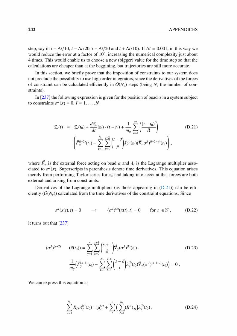
242 APPENDICES
step, say in t − ∆t/10, t − ∆t/20, t + ∆t/20 and t + ∆t/10). If ∆t = 0.001, in this way wewould reduce the error at a factor of 106, increasing the numerical complexity just about4 times. This would enable us to choose a new (bigger) value for the time step so that thecalculations are cheaper than at the beggining, but trajectories are still more accurate.
In this section, we briefly prove that the imposition of constraints to our system doesnot preclude the possibility to use high order integrators, since the derivatives of the forcesof constraint can be calculated efficiently in O(Nc) steps (being Nc the number of con-straints).
In [237] the following expression is given for the position of bead α in a system subjectto constraints σI(x) = 0, I = 1, . . . ,Nc
~xα(t) = ~xα(t0) +d~xαdt
(t0) · (t − t0) +1
mα
∞∑l=2
((t − t0)l
l!
)(D.21) ~F(l−2)
α (t0) −Nc∑I=1
l−2∑p=0
(l − 2
p
)λ
(p)I (t0)(~∇ασI)(l−2−p)(t0)
,where ~Fα is the external force acting on bead α and λI is the Lagrange multiplier asso-ciated to σI(x). Superscripts in parenthesis denote time derivatives. This equation arisesmerely from performing Taylor series for xα and taking into account that forces are bothexternal and arising from constraints.
Derivatives of the Lagrange multipliers (as those appearing in (D.21)) can be effi-ciently (O(Nc)) calculated from the time derivatives of the constraint equations. Since
σI(x(t), t) = 0 ⇒ (σI)(s)(x(t), t) = 0 for s ∈ N , (D.22)
it turns out that [237]
(σI)(s+2) (~x(t0)) =
n∑γ=1
s+1∑k=0
(s + 1
k
)~∇γ(σI)(k)(t0) · (D.23)
1mγ
(~F(s−k)γ (t0) −
Nc∑J=1
s−k∑l=0
(s − k
l
)λ(l)
J (t0)~∇γ(σJ)(s−k−l)(t0))
= 0 ,
We can express this equation as
Nc∑J=1
RIJλ(s)J (t0) = µ(s)
I +
∗∑l
( Nc∑J=1
(R′l)
JI
)λ(l)
J (t0) , (D.24)

D EFFICIENT CALCULATION OF DERIVATIVES OF LAGRANGEMULTIPLIERS INTO ROBOTICS 243
where
RJI :=n∑ζ=1
1mζ
~∇ζσJ(t0)~∇lσ
I(t0) , (D.25a)
µ(s)I :=
n∑ζ=1
s+1∑k=1
1mζ
~F(s−k)ζ (t0)~∇ζ(σI)(k)(t0) , (D.25b)
(R′l)
JI :=n∑ζ=1
∑k
(s + 1
k
)(s − k
l
)( 1mζ
)~∇ζ(σJ)(s−k−l)(t0)~∇ζ(σI)(k)(t0) . (D.25c)
The asterisk in the superscript of∑∗
l means that the term k = 0, l = s is to be skipped.Therefore
R~λ(s) = ~µ + R′1~λ(1) + R′2~λ(2) + . . . + R′s−1~λ(s−1) . (D.26)
Using (9.8), (D.25a) turn to (9.15), as seen in sec. 9.2. Provided that σI(α,β) := ( ~xα−~xβ)2−
(aα,β)2, σJ(γ,ε) := ( ~xγ − ~xε)2 − (aγ,ε)2, eqs. (D.25b) and (D.25c) become
µ(s)I = 2
s+1∑k=1
( ~F(s−k)α
mα
−
~F(s−k)β
mβ
)(~x(k)
α − ~x(k)β ) , (D.27a)
(R′l)
JI =
s+1∑k=0
(s + 1
k
)(s − k
l
)(~x(s−k−l)
γ − ~x(s−k−l)ε ) · (~x(k)
α − ~x(k)β )(
δαγ
mα
−δβγ
mβ
−δαεmα
+δβε
mβ
), (D.27b)
where ~F(−1)α := mαd~xα/dt. So every row of vector ~µ can be obtained in order s + 1 op-
erations (being s the order of the derivative of the Lagrange multipliers we are lookingfor) and R′ is a sparse matrix with the same zero entries that the R matrix calculated inprevious sections for logical geometries. Hence the product of R′l by any vector can beagain obtained again in Nc operations (where Nc is the number of rows of this vector).Equations (D.24), (D.25) and (D.26) ensure that the Nc × 1 vector of the s-th derivative ofthe Lagrange multipliers sought ~λ(s) can be obtained in order Nc · (s + 1) operations, thuspreventing the number of calculations to scale with the square or cube of any magnitude.The previous equations are the generalization of (9.14).
Let’s see an example of a possible Algorithm 7 (of third order). Its scheme is asfollows. We could use a procedure to re-calculate positions of order above 2:
~xα(t0 + ∆t) = ~xα(t0) +d~xα(t0)
dt∆t +
+1
mα
(~Fα(t0) +
∑I
λI~∇ασI(t0)
)∆t2 +
+1
mα
(d ~Fα(t0)dt
+∑
I
γI~∇ασI(t0) +
∑I
λI
∑β
∂2σI(t0)∂β∂α
~xβ(t0)dt
)∆t3 (D.28)

244 APPENDICES
where we have used that
dσI(t0)dt
=∑β
~∇βσI(t0)
d~xβ(t0)dt
. (D.29)
γI are a set of parameters that sustitute dλI (t0)dt in (D.28). They are arbitrarily arranged for ~x
not to leave the constrained subspace. They are to be obtained through σI(~x(t0 + ∆t)) = 0.This can be done with a method analogous to SHAKE [237]. The higher order of thismethod allows to increase the time step with respect to algorithms of lower order.
We have just introduced the scheme of a method of order 3. However, the concept itis based on can be used to build methods of any order. These methods will require deriva-tives of the forces and of the Lagrange multipliers (see (D.28)), that can be calculatedusing the values of variables in previous times in difference quotients.

Acronyms
ALDA Adiabatic Local Density Approximation. 28
ALU arithmetic-logic unit. 44
BO Born-Oppenheimer. 9
CC Coupled Cluster. 10
CI Configuration Interaction. 10
CPU Central Process Unit. 44
CT charge transfer. 82, 89–91
DFT Density Functional Theory. 10, 11
FFT Fast Fourier Transform. 67
FMM Fast Multipole Method. 67
FoR Frame of Reference. 102–104
GFP Green Fluorescent Protein. 81–83, 92
GGA Generalized Gradient Approximation. 22
GLY3 N-acetyl-glycyl-glycyl-glycyl-amide. 108, 110, 111
HBDI 4-hydroxybenzylidene-2,3-dimethyl-imidazolinone. 81
HEG Homogeneous Electron Gas. 21
HF Hartree-Fock. 10
HPC High Performance Computing. 43, 63
KS Kohn-Sham. 11, 27
LCAO Linear Combination of Atomic Orbitals. 90, 92, 221
LDA Local Density Approximation. 20

246 Acronyms
MC Monte Carlo. 34, 37
MCSCF Multi Configuration Self Consistent Field. 10
MD Molecular Dynamics. 34, 35, 37, 112, 131
MM Molecular Mechanics. 31, 33, 35
MMT mass-metric tensor. 128, 141, 142, 145, 146, 148, 153, 158–160, 162, 163
MP Møller-Plesset. 10
NMA N-methyl-acetamide. 108, 111
PDF equilibrium probability density function. 129–131, 133–136, 141–143, 147–149,151, 154, 156–159, 169
QM Quantum Mechanics. 5, 10, 33
QM/MM Quantum Mechanics/Molecular Mechanics. 31, 83
TDDFT Time-dependent Density Functional Theory. 10, 25

Bibliography
[1] P. Garcia-Risueno and P. Echenique, Linearly scaling direct method for accurately invertingsparse banded matrices, Accepted by the J. of Phys. A: Math. and Theor. (2011) , http://arxiv.org/abs/1009.0938. 194, 197, 200, 201, 207, 214, 215, 239, 241
[2] P. Garcia-Risueno, P. Echenique, and J. L. Alonso, Exact and efficient calculation of La-grange multipliers in constrained biological polymers: Proteins and nucleic acids as exam-ple cases, J. Comput. Chem. 32 (2011) 3039–3046. 169
[3] P. Echenique, C. N. Cavasotto, M. De Marco, P. Garcia-Risueno, and J. L. Alonso, Anexact expression to calculate the derivatives of position-dependent observables in molecularsimulations with flexible constraints, PLoS ONE 6(9): e24563, 2010. 135, 137
[4] P. Echenique, C. N. Cavasotto, and P. Garcia-Risueno, The canonical equilibrium of con-strained molecular models, Eur. Phys. J. ST 200 (2011) 5–54, http://arxiv.org/abs/1105.0374. 96, 97, 98, 100, 102, 104, 117
[5] M. Wanko, P. Garcia-Risueno, and A. Rubio, Excited States of the Green FluorescentProtein Chromophore: Performance of Ab Initio and Semi-Empirical Methods, Phys. StatusSolidi (Special Issue) (2011) , DOI 10.1002/pssb.201100536. 81
[6] A. Castro, H. Appel, M. Oliveira, C. A. Rozzi, X. Andrade, F. Lorenzen, M. A. L. Mar-ques, E. K. U. Gross, and A. Rubio, Octopus: a tool for the application of time-dependentdensity functional theory, Phys. Stat. Sol 243 (2006) 2465. iv, viii, 3, 23, 25, 30, 31, 37,66, 169, 219
[7] P. A. M. Dirac, Quantum Mechanics of Many-Electron Systems’, Proceedings of the RoyalSociety 123 (1929) 714–733. 1
[8] S. Reich, Smoothed Langevin dynamics of highly oscillatory systems, Physica D 118 (2000)210–224. 2, 156, 157
[9] D. E. Shaw, R. Ron O. Dror, J. Salmon, J. Grossman, K. Mackenzie, J. Bank, C. Young,B. Batson, K. Bowers, E. Edmond Chow, M. Eastwood, D. Ierardi, J. John L. Klepeis,J. Jeffrey S. Kuskin, R. Larson, K. Kresten Lindorff-Larsen, P. Maragakis, M. M.A.,S. Piana, S. Yibing, and B. Towles, Millisecond-Scale Molecular Dynamics Simulationson Anton, In Proceedings of the ACM/IEEE Conference on Supercomputing (SC09), ACMPress, New York, (2009) . 2, 33, 58, 193, 207
[10] V. S. Pande, I. Baker, J. Chapman, S. P. Elmer, S. Khaliq, S. M. Larson, Y. M. Rhee, M. R.Shirts, C. D. Snow, E. J. Sorin, and B. Zagrovic, Atomistic protein folding simulationson the submillisecond time scale using worldwide distributed computing, Biopolymers 68(2003) 91–109. 2, 54, 63
[11] T. Guo-Quing, R. P. Bandwar, and S. S. Patel, Extended Upstream A-T Sequence IncreasesT7 Promoter Strength, J. Biol. Chem. 280 (2005) 40707–40713. 2

248 BIBLIOGRAPHY
[12] B. Rotenberg, M. Salanne, C. Simon, and R. Vuilleumier, From Localized Orbitals toMaterial Properties: Building Classical Force Fields for Nonmetallic Condensed MatterSystems, Phys. Rev. Lett. 104 (2010) 138301. 2, 33
[13] C. J. Cramer, Essentials of Computational Chemistry: Theories and Models, John Wiley& Sons, Chichester, 2nd edition, 2002. 2, 10, 30, 31, 32, 34
[14] T. C. Germann, K. Kadau, and S. Swaminarayan, 369 Tflop/s molecular dynamics simula-tions on the petaflop hybrid supercomputer ”Roadrunner”, Concurrency and Computation:Practice and Experience 21 (2009) 2143–2159. 2, 35, 42, 50, 53, 61
[15] M. A. L. Marques, X. Lopez, D. Varsano, A. Castro, and A. Rubio, Time-DependentDensity-Functional Approach for Biological Chromophores: The Case of the Green Fluo-rescent Protein, Phys. Rev. Lett. 90 (2003) 258101. 3
[16] D. E. Shaw, R. O. Dror, J. K. Salmon, J. P. Grossmann, K. M. Mackenzie, J. A. Bank,C. Young, M. M. Deneroff, B. Batson, K. J. Bowers, E. Chow, M. P. Eastwood, D. J.Ierardi, J. L. Klepeis, J. S. Kuskin, R. H. Larson, K. Lindorff-Larsen, P. Maragakis,M. A. Moraes, S. Piana, Y. Shan, and B. Towles, Millisecond-scale molecular dynamicssimulations on Anton, in Proceedings of the ACM/IEEE Conference on Supercomputing(SC09), pp. 14–20, Portland, Oregon, 2009. 3, 35, 119
[17] D. Marx, Proton Transfer 200 Years after von Grotthuss: Insights from Ab Initio Simula-tions, ChemPhysChem 7 (2006) 1848–1870. 3
[18] W. D. Cornell, P. Cieplak, C. I. Bayly, I. R. Gould, J. Merz, K. M., D. M. Ferguson, D. C.Spellmeyer, T. Fox, J. W. Caldwell, and P. A. Kollman, A second generation force fieldfor the simulation of proteins, nucleic acids, and organic molecules, J. Am. Chem. Soc.117 (1995) 5179–5197. 3, 111, 163
[19] P. Hobza and J. Sponer, Structure, Energetics, and Dynamics of the Nucleic Acid Base PairsNonempirical Ab Initio Calculations, Chemical Reviews 99 (1999) 3247-3276. 3
[20] G. Kresse and J. Hafner, Ab initio molecular dynamics for liquid metals, Phys. Rev. B 47(1993) 558–561. 3
[21] R. Dovesi, B. Civalleri, C. Roetti, V. R. Saunders, and R. Orlando, Ab Initio QuantumSimulation in Solid State Chemistry, pp. 1–125, John Wiley & Sons, Inc., 2005. 3
[22] P. Gibbon, R. Speck, A. Karmakar, L. Arnold, W. Frings, B. Berberich, D. Reiter, andM. Masandek, Progress in Mesh-Free Plasma Simulation With Parallel Tree Codes, PlasmaScience, IEEE Transactions on 38 (2010) 2367–2376. 3
[23] G. Vidal, Efficient Simulation of One-Dimensional Quantum Many-Body Systems, Phys.Rev. Lett. 93 (2004) 040502. 3
[24] G. Kresse and J. Furthmller, Efficiency of ab-initio total energy calculations for metals andsemiconductors using a plane-wave basis set, Computational Materials Science 6 (1996)15 - 50. 3
[25] H. Katayama-Yoshida and K. Sato, Materials design for semiconductor spintronics by abinitio electronic-structure calculation, Physica B: Condensed Matter 327 (2003) 337 - 343.3
[26] A. H. Castro-Neto, F. Guinea, N. M. R. Peres, K. S. Novoselov, and A. K. Geim, Theelectronic properties of graphene, Rev. Mod. Phys. 81 (2009) 109–162. 3
[27] M. Shapiro and P. Brumer, Principles of the Quantum Control of Molecular Processes,Wiley-VCH, 2003. 3
BIBLIOGRAPHY 249
[28] G. Vidal, Efficient Classical Simulation of Slightly Entangled Quantum Computations,Phys. Rev. Lett. 91 (2003) 147902. 3
[29] J. I. Cirac and P. Zoller, Quantum Computations with Cold Trapped Ions, Phys. Rev. Lett.74 (1995) 4091–4094. 3
[30] R. A. Friesner and V. Guallar, Ab initio quantum chemical amd mixed Quantum Me-chanics/Molecular Mechanics (QM/MM) methods for studyng enzymatic catalysis, AnnualReview of Physical Chemistry 56 (2005) 389-427. 3
[31] B. Fischer, K. Fukuzawa, and W. Wenzel, Receptor-specific scoring functions derived fromquantum chemical models improve affinity estimates for in-silico drug discovery, Proteins:Structure, Function, and Bioinformatics 70 (2008) 1264–1273. 3
[32] J. H. Lin, A. L. Perryman, J. R. Schames, and J. A. McCammon, Computational drug designaccommodating receptor flexibility: The relaxed complex scheme, J. Am. Chem. Soc. 124(2002) 5632-5633. 3
[33] A. S. Barnard, How can ab initio simulations address risks in nanotech?, Nature Nan-otechnology 4 (2009) 332–335. 3
[34] M. Zimmer, GFP: from jellyfish to the Nobel prize and beyond, Chem. Soc. Rev. 38 (2009)2823-2832. 3, 23, 81
[35] R. Y. Tsien, The Green Fluorescent Protein, Annual review of biochemistry 67 (1998)509–544. 3, 23, 81
[36] C. Cohen-Tannoudji, B. Diu, and F. Laloe, Quantum Mechanics, Hermann and John Wiley& Sons, Paris, 2nd edition, 1977. 5
[37] W. Greiner, Relativistic Quantum Mechanics, Wave Equations, Springer-Verlag, 1990. 6
[38] D. E. Kharzeev and D. T. Son, Testing the Chiral Magnetic and Chiral Vortical Effects inHeavy Ion Collisions, Phys. Rev. Lett. 106 (2011) 062301. 7, 8
[39] A. J. Baltz, Exact Dirac Equation Calculation of Ionization and Pair Production Inducedby Ultrarelativistic Heavy Ions, Phys. Rev. Lett. 78 (1997) 1231–1234. 7
[40] J. Lindhard and A. H. So/rensen, Relativistic theory of stopping for heavy ions, Phys. Rev.A 53 (1996) 2443–2456. 7
[41] H. Nakashima and H. Nakatsuji, How Accurately Does the Free Complement Wave Func-tion of a Helium Atom Satisfy the Schrödinger Equation?, Phys. Rev. Lett. 101 (2008)240406. 7
[42] H. Frauenfelder, P. G. Wolynes, and R. H. Austin, Biological Physics, Rev. Mod. Phys.71 (1999) S419–S430. 7
[43] W. Kohn, An essay on condensed matter physics in the twentieth century, Rev. Mod. Phys.71 (1999) S59–S77. 7
[44] J. Gonzalez, F. Guinea, and M. A. H. Vozmediano, The electronic spectrum of fullerenesfrom the Dirac equation, Nucl. Phys. B 406 (1993) 771–794. 7
[45] R. Jackiw, A. I. Milstein, S.-Y. Pi, and I. S. Terekhov, Induced current and Aharonov-Bohmeffect in graphene, Phys. Rev. B 80 (2009) 033413. 7
[46] W. Greiner, Quantum Mechanics, An introduction, Springer-Verlag, 1989. 7
[47] R. Eisberg and R. Resnick, Física cuántica: átomos, moléculas, sólidos, núcleos y partícu-las, Limusa Noriega Editores, 1985. 8
250 BIBLIOGRAPHY
[48] J. R. Vazquez de Aldana and L. Roso, Spin effects in the interaction of atoms with intenseand high-frequency laser fields in the non-relativistic regime, J. Phys. B: At. Mol. Opt.Phys. 33 (2000) 3701. 8
[49] S. Furuta, C. H. W. Barnes, and C. J. L. Doran, Single-qubit gates and measurements inthe surface acoustic wave quantum computer, Phys. Rev. B 70 (2004) 205320. 8
[50] P. Echenique and J. L. Alonso, A mathematical and computational review of Hartree-FockSCF methods in Quantum Chemistry, Mol. Phys. 105 (2007) 3057–3098. 9, 10, 11, 18, 98,101, 117, 120, 138, 170
[51] F. Jensen, Introduction to Computational Chemistry, John Wiley & Sons, Chichester, 1998.10, 22, 25, 30, 31, 35, 100, 101, 120
[52] H. Eschrig, The fundamentals of Density Functional Theory, Eagle, Leipzig, 2nd edition,2003. 10, 11, 16
[53] J. L. Alonso, Notes on Density Functional Theory, 2011, Dept. de Física Teórica, Univer-sidad de Zaragoza. 10
[54] R. G. Parr and W. Yang, Density Functional Theory of Atoms and Molecules, Oxford, NewYork, 1989. 10, 18, 20, 21, 22, 25, 27, 66
[55] R. Van Leeuwen and E. K. U. Gross, in Time-Dependent Density Functional Theory, editedby M. A. L. Marques, C. A. Ullrich, F. Nogueira, A. Rubio, K. Burke, and E. K. U. Gross,Springer, 2006. 11
[56] P. Hohenberg and W. Kohn, Inhomogeneous Electron Gas, Phys. Rev. 136 (1964) B864–B871. 13
[57] K. Capelle, C. A. Ullrich, and G. Vignale, Degenerate ground states and nonuniquepotentials: Breakdown and restoration of density functionals, Phys. Rev. A 76 (2007)012508. 15, 16
[58] J. E. Harriman, Geometry of density matrices. IV. The relationship between density matricesand densities, Phys. Rev. A 27 (1983) 632–645. 16
[59] W. Kohn and L. J. Sham, Self-Consistent Equations Including Exchange and CorrelationEffects, Phys. Rev. 140 (1965) A1133–A1138. 16
[60] J. P. Perdew, A. Ruzsinszky, L. A. Constantin, J. Sun, and G. I. Csonka, Some Fundamen-tal Issues in Ground-State Density Functional Theory: A Guide for the Perplexed, J. Chem.Theory Comput. 5 (2009) 902-908. 17, 19, 20, 21
[61] R. M. Dreizler and E. K. U. Gross, Density Functional Theory, Springer Verlag Heidel-berg, 1990. 20
[62] W. Kohn and L. J. Sham, Self-consistent equations including exchange and correlationeffects, Phys. Rev. 140 (1965) A1133–A1138. 20
[63] J. P. Perdew, K. Burke, and M. Ernzerhof, Generalized gradient approximation madesimple, PRL 77 (1996) 3865. 20, 25, 26
[64] P. J. Stephens, F. J. Devlin, C. F. Chabalowski, and M. J. Frisch, Ab initio calculation ofvibrational absorption and circular dichroism spectra using density functional force fields,J. Phys. Chem. 98 (1994) 11623–11627. 20, 22
[65] J. P. Perdew and A. Zunger, Self-interaction correction to density-functional approxima-tions for many-electron systems, Phys. Rev. B 23 (1981) 5048–5079. 21
[66] L. A. Cole and J. P. Perdew, Calculated electron affinities of the elements, Phys. Rev. A 25(1982) 1265–1271. 21
BIBLIOGRAPHY 251
[67] J. P. Perdew and Y. Wang, Accurate and simple analytic representation of the electron-gascorrelation energy, Phys. Rev. B 45 (1992) 13244–13249. 21
[68] L. Hedin and B. I. Lundqvist, Explicit local exchange-correlation potentials, Journal ofPhysics C: Solid State Physics 4 (1971) 2064. 21
[69] S. H. Vosko, L. Wilk, and M. Nusair, Accurate spin-dependent electron liquid correlationenergies for local spin density calculations: a critical analysis, Can. J. Phys. 58 (1980)1200–1211. 21, 22, 23, 25, 26
[70] W. Koch and M. C. Holthausen, A chemist’s guide to Density Functional Theory, Wiley,1999. 21
[71] W. J. Carr, Energy, Specific Heat, and Magnetic Properties of the Low-Density ElectronGas, Phys. Rev. 122 (1961) 1437–1446. 22
[72] W. J. Carr and A. A. Maradudin, Ground-State Energy of a High-Density Electron Gas,Phys. Rev. 133 (1964) A371–A374. 22
[73] W. Kohn, Y. Meir, and D. E. Makarov, van der Waals Energies in Density FunctionalTheory, Phys. Rev. Lett. 80 (1998) 4153–4156. 22
[74] J. P. Perdew, K. Burke, and M. Ernzerhof, Generalized gradient approximation madesimple, PRL 78 (1997) 1396(E). 22, 25, 26
[75] A. D. Becke, A multicenter numerical integration scheme for polyatomic molecules, J.Chem. Phys. 88 (1988) 2547. 23
[76] J. P. Perdew, in Electronic Structure of Solids, edited by P. Ziesche and H. Eschrig,Akademie Verlag, Berlin, 1991. 23
[77] R. M. Martin, Electronic Structure, Cambridge University Press, 2004. 24
[78] A. Kokalj, Computer graphics and graphical user interfaces as tools in simulations ofmatter at the atomic scale, Comp. Mat. Sci. 28 (2003) 155–168, http://www.xcrysden.org. 23
[79] L. A. Curtiss, K. Raghavachari, P. C. Redfern, and J. A. Pople, Assessment of Gaussian-2and density functional theories for the computation of enthalpies of formation, J. Chem.Phys. 106 (1997) 1063. 23
[80] V. M. Oltedal, Thesis for the Degree of Doctor Scientiarum: Chemical Insights from Car-bon 1s Photoelectron Spectroscopy and Theoretical Modeling, Department of Chemistry -University of Bergen, 2007. 25
[81] D. R. Bowler and T. Miyazaki, Calculations for millions of atoms with density functionaltheory: linear scaling shows its potential, J. Phys. Condens. Matter 22 (2010) 074207. 25
[82] J. M. Soler, E. Artacho, J. D. Gale, A. Garcia, J. Junquera, P. Ordejon, and D. Sanchez-Portal, The SIESTA method for ab initio order- N materials simulation, Journal of Physics:Condensed Matter 14 (2002) 2745. 25, 170
[83] N. Hine, P. Haynes, A. Mostofi, C.-K. Skylaris, and M. Payne, Linear-scaling density-functional theory with tens of thousands of atoms: Expanding the scope and scale of cal-culations with ONETEP, Computer Physics Communications 180 (2009) 1041 - 1053. 25,170
[84] W. A. de Jong, E. Bylaska, N. Govind, C. L. Janssen, K. Kowalski, T. Muller, I. M. B.Nielsen, H. J. J. van Dam, V. Veryazov, and R. Lindh, Utilizing high performance computingfor chemistry: parallel computational chemistry, Phys. Chem. Chem. Phys. 12 (2010)6896–6920. 25, 46, 50, 52, 54, 56, 57, 193

252 BIBLIOGRAPHY
[85] E. Runge and E. K. U. Gross, Density-Functional Theory for Time-Dependent Systems,Phys. Rev. Lett. 52 (1984) 997. 27
[86] E. K. U. Gross and W. Kohn, in Density Functional Theory of many-fermion systems, editedby P.-O. Lowdin and S. B. Trickey, Elsevier, Adv. Quant. Chem 21, 1990. 27, 30
[87] M. E. Casida and M. Huix-Rotllant, Progress in Time-Dependent Density-FunctionalTheory (2011) , arXiv:1108.0611v1. 27, 28, 66
[88] E. K. U. Gross and K. Burke, in Time-Dependent Density Functional Theory, edited byM. A. L. Marques, C. A. Ullrich, F. Nogueira, A. Rubio, K. Burke, and E. K. U. Gross,Springer, 2006. 28, 29, 66
[89] M. Plischke and B. Bergersen, Equilibrium Statistical Physics, World Scientific, 3rdedition, 2005. 29
[90] N. L. Doltsinis, in Computational Nanoscience: Do It Yourself!, edited by J. Grotendorst,S. Blugel, and D. Marx, volume 31, pp. 357–373, NIC Series, John von Neumann Institutefor Computing, Jülich, 2006. 30
[91] M. C. Zerner, Semiempirical Molecular Orbital Methods, in Reviews in ComputationalChemistry vol. 2, pp. 313–365, John Wiley & Sons, Inc., 1991. 31
[92] P. Echenique and J. L. Alonso, Definition of Systematic, Approximately Separable and Mod-ular Internal Coordinates (SASMIC) for macromolecular simulation, J. Comput. Chem. 27(2006) 1076–1087. 31, 103, 104, 107, 108, 109, 110, 123, 127, 129, 130, 135, 142, 150,159, 163
[93] C. Oostenbrink, A. Villa, A. E. Mark, and W. F. van Gunsteren, A Biomolecular ForceField Based on the Free Enthalpy of Hydration and Solvation: The GROMOS Force-FieldParameter Sets 53A5 and 53A6, J. Comput. Chem 26 (2005) 1719–1751. 32, 33
[94] H. Cheng, L. F. Greengard, and V. Rokhlin, A new version of the fast multipole method forthe Laplace equation in three dimensions, J. Comp. Phys 155 (1999) 468–498. 33, 70
[95] L. F. Greengard and V. Rokhlin, A fast algorithm for particle simulations, J. Comp. Phys.73 (1987) 325. 33, 70
[96] T. A. Darden, D. York, and L. Pedersen, Particle mesh Ewald: An N log(N) method forEwald sums in large systems, J. Chem. Phys. 98 (1993) 10089–10092. 33, 74, 101
[97] J. W. Cooley and J. W. Tukey, An algorithm for the machine calculation of complex Fourierseries, Math. Comput. 19 (1965) 297–301. 33, 67
[98] Q. Lu and R. Luo, A Poisson-Boltzmann dynamics method with nonperiodic boundarycondition, J. Chem. Phys. 119 (2003) 11035–11047. 33
[99] J. W. Ponder and D. A. Case, Force fields for protein simulations, Adv. Prot. Chem. 66(2003) 27–85. 33, 98, 100, 101, 120, 137
[100] M. Rueda, C. Ferrer-Costa, T. Meyer, A. Perez, J. Camps, A. Hospital, J. L. Gelpi, andM. Orozco, A consensus view of protein dynamics, Proc. Natl. Acad. Sci. USA 104,3(2007) 796–801. 33
[101] S. A. Harris, E. Gavathiotis, M. S. Searle, M. Orozco, and C. A. Laughton, Cooperativityin Drug-DNA Recognition: A Molecular Dynamics Study, JACS 123 (2001) 12658–12663.33
[102] M. Orozco and F. J. Luque, The impact of theoretical chemistry on biology, Contributionsto Science 6 (2010) 133–142. 33

BIBLIOGRAPHY 253
[103] M. Zimmer, Are classical molecular mechanics calculations still useful in bioinorganic sim-ulations?, Coordination Chemistry Reviews 253 (2009) 817 - 826, Theory and Computingin Contemporary Coordination Chemistry. 33
[104] P. Comba and M. Kerscher, Computation of structures and properties of transition metalcompounds, Coordination Chemistry Reviews 253 (2009) 564 - 574, Theory and Comput-ing in Contemporary Coordination Chemistry. 33
[105] D. Frenkel and B. Smit, Understanding Molecular Simulation, Academic Press - HarcourtInc., 2nd edition, 2002. 34, 35, 37
[106] B. Leimkuhler and S. Reich, Simulating Hamiltonian dynamics, Cambridge UniversityPress - Cambridge monographs on applied and computational Mathematics, 1st edition,2004. 34, 189
[107] M. P. Allen and D. J. Tildesley, Computer simulation of liquids, Clarendon Press, Oxford,2005. 34, 95, 119, 138
[108] J. C. Phillips, R. Braun, W. Wei, J. Gumbart, E. Tajkhorshid, E. Villa, C. Chipot, R. D.Skeel, L. Kale, and K. Schulten, Scalable molecular dynamics with NAMD, JCC 26,16(2005) 1781–1802. 34, 35, 36, 193
[109] L. Verlet, Computer ”experiments” on classical fluids. I. Thermodynamical properties ofLennard-Jones molecules, Phys. Rev. 159 (1967) 98–103. 35, 193
[110] D. Frenkel, Monte Carlo simulations and molecular dynamics, 2007,http://www.jncasr.ac.in/ccms/ums2007/lecturenotes/Bangalore07.pdf. 35
[111] K. Y. Sanbonmatsu and C.-S. Tung, High performance computing in biology: Multimillionatom simulations of nanoscale systems, Journal of Structural Biology 157 (2007) 470 - 480,Advances in Molecular Dynamics Simulations. 35
[112] N. Metropolis, A. N. Rosenbluth, M. N. Rosenbluth, A. H. Teller, and E. Teller, Equa-tion of state calculation by fast computing machines, J. Chem. Phys. 21 (1953) 1087–1092.37
[113] D. A. Case, T. A. Darden, T. E. Cheatham III, C. L. Simmerling, J. Wang, R. E. Duke,R. Luo, M. Crowley, R. C. Walker, W. Zhang, K. M. Merz, B. Wang, S. Hayik, A. Roit-berg, G. Seabra, I. Kolossvary, K. F. Wong, F. Paesani, J. Vanicek, X. Wu, S. R. Brozell,T. Steinbrecher, H. Gohlke, L. Yang, C. Tan, J. Mongan, V. Hornak, G. Cui, D. H. Math-ews, M. G. Seetin, C. Sagui, V. Babin, and P. A. Kollman, AMBER 11 User’s Manual,University of California, San Francisco, 2010. 37
[114] D. van der Spoel, E. Lindahl, B. Hess, G. Groenhof, A. E. Mark, and H. J. C. Berendsen,GROMACS: fast, flexible and free, J. Comput. Chem. 26 (2005) 1701–1719. 37, 217
[115] B. R. Brooks, C. L. Brooks III, A. D. MacKerell, L. Nilsson, R. J. Petrella, B. Roux,Y. Won, G. Archontis, C. Bartels, S. Boresch, A. Caflisch, L. Caves, C. Cui, A. R. Din-ner, M. Feig, S. Fischer, J. Gao, M. Hodoscek, W. Im, K. Kuczera, T. Lazaridis, J. Ma,V. Ovchinnikov, E. Paci, R. W. Pastor, C. B. Post, J. Z. Pu, M. Schaefer, B. Tidor, R. M.Venable, H. L. Woodcock, X. Wu, W. Yang, D. M. York, and M. Karplus, CHARMM:The biomolecular simulation program, J. Comput. Chem. 30 (2009) 1545–1615. 37, 98,101, 120, 137
[116] K. J. Bowers, E. Chow, H. Xu, R. O. Dror, M. P. Eastwood, B. A. Gregersen, J. L.Klepeis, I. Kolossvary, M. A. Moraes, F. D. Sacerdoti, J. K. Salmon, Y. Shan, and D. E.Shaw, Scalable algorithms for molecular dynamics simulations on commodity clusters, inProceedings of the 2006 ACM/IEEE conference on Supercomputing, SC ’06, New York,NY, USA, 2006, ACM. 37

254 BIBLIOGRAPHY
[117] M. Valiev, E. Bylaska, N. Govind, K. Kowalski, T. Straatsma, H. V. Dam, D. Wang,J. Nieplocha, E. Apra, T. Windus, and W. de Jong, NWChem: A comprehensive andscalable open-source solution for large scale molecular simulations, Computer PhysicsCommunications 181 (2010) 1477 - 1489. 37, 66
[118] R. Car and M. Parrinello, Unified Approach for Molecular Dynamics and Density-Functional Theory, Phys. Rev. Lett. 55 (1985) 2471–2474. 37, 95, 120
[119] J. L. Alonso, X. Andrade, P. Echenique, F. Falceto, D. Prada-Gracia, and A. Rubio, Ef-ficient formalism for large-scale ab initio molecular dynamics based on time-dependentdensity functional theory, Phys. Rev. Lett. 101 (2008) 096403. 37, 117, 120, 170
[120] G. Makov, C. Gattinoni, and A. D. Vita, Ab initio based multiscale modelling for materialsscience, Modelling and Simulation in Materials Science and Engineering 17 (2009) 084008.39
[121] D. Goldberg, Appendix H: Computer Arithmetic, in Computer Architecture, A QuantitativeApproach, edited by J. L. Hennessy and D. A. Patterson, Morgan Kaufmann - Elsevier, SanMateo, CA, 2003. 39
[122] P. Shivakumar, M. Kistler, S. Keckler, D. Burger, and L. Alvisi, Modeling the effect oftechnology trends on the soft error rate of combinational logic, in Dependable Systems andNetworks, 2002. DSN 2002. Proceedings. International Conference on, pp. 389–398, 2002.41
[123] G. M. Amdahl, Validity of the single processor approach to achieving large scale computingcapabilities, in Proceedings of the April 18-20, 1967, spring joint computer conference,AFIPS ’67 (Spring), pp. 483–485, New York, NY, USA, 1967, ACM. 42
[124] G. Hager and G. Wellein, Introduction to High Performance Computing for Scientists andEngineers, CRC Press - Taylor & Francis Group, 1st edition, 2011. 43, 44, 45, 46, 47, 50,52, 53, 54, 55, 56, 61, 184
[125] J. Haoqiang, D. Jespersen, P. Mehrotra, R. Biswas, H. Lei, and B. Chapman, High perfor-mance computing using MPI and OpenMP on multi-core parallel systems, Parallel Com-puting In Press, Corrected Proof (2011) . 43, 54, 57
[126] J. L. Hennessy and D. A. Patterson, Computer Architecture, A Quantitative Approach,Morgan Kaufmann - Elsevier, San Mateo, CA, 3rd edition, 2003. 45, 183, 184
[127] R. Wood, Future hard disk drive systems, Journal of Magnetism and Magnetic Materials321 (2009) 555 - 561, Current Perspectives: Perpendicular Recording. 46
[128] J. Gray, D. T. Liu, M. Nieto-Santisteban, A. Szalay, D. J. DeWitt, and G. Heber, Scientificdata management in the coming decade, SIGMOD Rec. 34 (2005) 34–41. 46, 62
[129] J. Larus, Spending Moore’s dividend, Commun. ACM 52 (2009) 62–69. 46, 47, 48, 49,61, 66
[130] M. N. Baibich, J. M. Broto, A. Fert, F. N. Van Dau, F. Petroff, P. Etienne, G. Creuzet,A. Friederich, and J. Chazelas, Giant Magnetoresistance of (001)Fe/(001)Cr MagneticSuperlattices, Phys. Rev. Lett. 61 (1988) 2472–2475. 46
[131] C. Chappert, A. Fert, and F. N. Van Dau, The emergence of spin electronics in data storage,Nat. Mater. 6 (2007) 813–823. 46
[132] G. Sun, X. Dong, Y. Xie, J. Li, and Y. Chen, in A novel architecture of the 3D stackedMRAM L2 cache for CMPs in IEEE 15th International Symposium on High PerformanceComputer Architecture, pp. 239–249, IEEE, 2009. 46
BIBLIOGRAPHY 255
[133] Y. Jin and K. Li, An optimal multimedia object allocation solution in multi-powermodestorage systems, Concurrency and Computation: Practice and Experience 22 (2010) 1852–1873. 46
[134] K. Olukotun and L. Hammond, The Future of Microprocessors, Queue 3 (2005) 26–29. 46,47, 49, 54, 60, 61
[135] A. Buttari, J. Dongarra, J. Kurzak, J. Langou, P. Luszczek, and S. Tomov, The impact ofmulticore on math software, in Proceedings of the 8th international conference on Appliedparallel computing: state of the art in scientific computing, PARA’06, pp. 1–10, Berlin,Heidelberg, 2007, Springer-Verlag. 47, 48, 61
[136] S. Zhou, D. Duffy, T. Clune, M. Suarez, S. Williams, and M. Halem, The impact ofIBM Cell technology on the programming paradigm in the context of computer systems forclimate and weather models, Concurrency and Computation: Practice and Experience 21(2009) 2176–2186. 48, 58
[137] Intel, Intel 64 and IA-32 Architectures Software Developer’s Manual, 2011, Intel orderNumber: 325462-039US. 51
[138] C. Sosa and B. Knudson, IBM System Blue Gene Solution: Blue Gene/P Application De-velopment, IBM Redbooks, 2009. 56
[139] J. Dongarra, D. Walker, E. Lusk, M. Snir, W. Gropp, A. Geist, S. Otto, R. Hempel,J. Cownie, T. Skjelum, L. Clarke, R. Littlefield, M. Sears, and S. Huss-Lederman, MPI:A Message-Passing Interface Standard, University of Tennessee, Knoxville, Tennessee, 4thedition, 2003. 56
[140] R. Kumar, D. Tullsen, N. Jouppi, and P. Ranganathan, Heterogeneous chip multiproces-sors, Computer 38 (2005) 32–38. 57
[141] E. Lindholm, J. Nickolls, S. Oberman, and J. Montrym, NVIDIA Tesla: A Unified Graphicsand Computing Architecture, Micro, IEEE 28 (2008) 39 -55. 57
[142] R. O. Dror, M. O. Jensen, D. W. Borhani, and D. E. Shaw, Exploring atomic resolutionphysiology on a femtosecond to millisecond timescale using molecular dynamics simula-tions, The Journal of Cell Biology 135 (6) (2010) 555–562. 58
[143] F. Belletti, M. Cotallo, A. Cruz, L. A. Fernandez, A. Gordillo-Guerrero, M. Guidetti,A. Maiorano, F. Mantovani, E. Marinari, V. Martin-Mayor, A. Munoz-Sudupe,D. Navarro, G. Parisi, S. Perez-Gaviro, M. Rossi, J. J. Ruiz-Lorenzo, S. F. Schifano,D. Sciretti, A. Tarancon, R. Tripiccione, J. L. Velasco, D. Yllanes, and G. Zanier, Janus:An FPGA-Based System for High-Performance Scientific Computing, Computing in Sci-ence and Engineering 11 (2009) 48-58. 58
[144] M. J., F. T., K. M., and N. K., GRAPE-6: The massively-parallel special-purpose computerfor astrophysical particle simulations, Publ. Astron. Soc. Japan 55 (2003) 1163. 58
[145] J. J. Dongarra, P. Luszczek, and A. Petitet, The LINPACK benchmark: Past, present andfuture, Concurrency and Computation: Practice and Experience 15 (2003) 803–820. 58
[146] B. Mohr, B. J. N. Wylie, and F. Wolf, Performance measurement and analysis tools forextremely scalable systems, Concurrency and computation: Practice and experience 22(2010) 2212–2229. 61
[147] D. H. Woo and H.-H. Lee, Extending Amdahl’s Law for Energy-Efficient Computing in theMany-Core Era, Computer 41 (2008) 24 -31. 61

256 BIBLIOGRAPHY
[148] J. Hamilton, CooperativeExpendableMicro-SliceServers (CEMS): Low Cost, Low PowerServers for Internet-Scale Services, Proc. 4th Biennial Conf. Innovative Data Systems Re-search (CIDR), Asilomar, CA, USA, January., 2009. 61
[149] L. Barroso and U. Holzle, The Case for Energy-Proportional Computing, Computer 40(2007) 33 -37. 61
[150] A. Berl, E. Gelenbe, M. d. Girolamo, G. Giuliani, H. De Meer, Q. D. Mihn, and K. Pen-tikousis, Energy-Efficient Cloud Computing, The Computer Journal 53 (2010) 1045–1051.61
[151] B. Wilkinson, Grid Computing: Techniques and Applications, Chapman & Hall/CRCComputational Science, 1st edition, 2009. 62
[152] M.-A. Thyveetil, P. V. Coveney, H. C. Greenwell, and J. L. Suter, Computer SimulationStudy of the Structural Stability and Materials Properties of DNA-Intercalated LayeredDouble Hydroxides, J. Am. Chem. Soc. 130 (2008) 4742-4756. 62
[153] D. Kondo, B. Javadi, P. Malecot, F. Cappello, and D. P. Anderson, Cost-benefit analysisof Cloud Computing versus desktop grids, Parallel and Distributed Processing Symposium,International 0 (2009) 1-12. 63, 64
[154] A. L. Beberg, D. L. Ensign, G. Jayachandran, S. Khaliq, and V. S. Pande, Folding@home:Lessons from eight years of volunteer distributed computing, Parallel and Distributed Pro-cessing Symposium, International 0 (2009) 1-8. 63
[155] C. Hoffa, G. Mehta, T. Freeman, E. Deelman, K. Keahey, B. Berriman, and J. Good, Onthe Use of Cloud Computing for Scientific Workflows, in eScience, 2008. eScience ’08.IEEE Fourth International Conference on, pp. 640 –645, 2008. 64
[156] I. Foster, Y. Zhao, I. Raicu, and S. Lu, Cloud Computing and Grid Computing 360-DegreeCompared, Grid Computing Environments Workshop, 2008. GCE ’08 (2009) 1–10. 64
[157] A. R. Leach, Molecular Modelling: principles and applications, Pearson Education -Prentice Hall, 2nd edition, 2001. 65
[158] M. H. Nayfeh and M. K. Brussel, Electricity and magnetism, John Wiley & sons, 1985. 65
[159] A. Castro, A. Rubio, and M. J. Stott, Solution of Poisson’s equation for finite systemsusing plane-wave methods, Canadian Journal of Physics 81 (2003) 1151–1164. 65, 68, 74
[160] J. Tomasi and M. Persico, Molecular Interactions in Solution: An Overview of MethodsBased on Continuous Distributions of the Solvent, Chemical Reviews 94 (1994) 2027-2094.65
[161] L. Genovese, T. Deutsch, A. Neelov, S. Goedecker, and G. Beylkin, Efficient solution ofPoisson’s equation with free boundary conditions, Journal of Chemical Physics 125 (2006)074105, Genovese, L. and Deutsch, T. and Neelov, A. and Goedecker, S. and Beylkin, G.66, 69, 70
[162] M. J. Frisch, G. W. Trucks, H. B. Schlegel, G. E. Scuseria, M. A. Robb, J. R. Cheese-man, G. Scalmani, V. Barone, B. Mennucci, G. A. Petersson, H. Nakatsuji, M. Caricato,X. Li, H. P. Hratchian, A. F. Izmaylov, J. Bloino, G. Zheng, J. L. Sonnenberg, M. Hada,M. Ehara, K. Toyota, R. Fukuda, J. Hasegawa, M. Ishida, T. Nakajima, Y. Honda, O. Ki-tao, H. Nakai, T. Vreven, J. A. Montgomery, Jr., J. E. Peralta, F. Ogliaro, M. Bearpark,J. J. Heyd, E. Brothers, K. N. Kudin, V. N. Staroverov, R. Kobayashi, J. Normand,K. Raghavachari, A. Rendell, J. C. Burant, S. S. Iyengar, J. Tomasi, M. Cossi, N. Rega,J. M. Millam, M. Klene, J. E. Knox, J. B. Cross, V. Bakken, C. Adamo, J. Jaramillo,R. Gomperts, R. E. Stratmann, O. Yazyev, A. J. Austin, R. Cammi, C. Pomelli, J. W.

BIBLIOGRAPHY 257
Ochterski, R. L. Martin, K. Morokuma, V. G. Zakrzewski, G. A. Voth, P. Salvador,J. J. Dannenberg, S. Dapprich, A. D. Daniels, O. Farkas, J. B. Foresman, J. V. Ortiz,J. Cioslowski, and D. J. Fox, Gaussian 09 Revision A.1, 2009, Gaussian Inc. WallingfordCT 2009. 66, 219
[163] V. Blum, R. Gehrke, F. Hanke, P. Havu, V. Havu, X. Ren, K. Reuter, and M. Scheffler,Ab initio molecular simulations with numeric atom-centered orbitals, Computer PhysicsCommunications 180 (2009) 2175 - 2196. 66, 219
[164] DelPhi Macromolecular Electrostatics Modelling Package, http://wiki.c2b2.columbia.edu/honiglab_public/index.php/Software:DelPhi. 66
[165] R. Ahlrichs, M. Bar, M. Haser, H. Horn, and C. Kolmel, Electronic structure calculationson workstation computers: The program system turbomole, Chemical Physics Letters 162(1989) 165 - 169. 66
[166] R. J. Needs, M. D. Towler, N. D. Drummond, and L.-R. P, CASINO Version 2.3 UserManual, University of Cambridge, Cambridge, UK, 2009. 66
[167] M. F. Guest, I. J. Bush, H. J. J. Van Dam, P. Sherwood, J. M. H. Thomas, J. H. Van Lenthe,R. W. A. Havenith, and J. Kendrick, The GAMESS-UK electronic structure package: algo-rithms, developments and applications, Mol. Phys. 6-8 (2005) 719–747. 66
[168] G. Karlstrom, R. Lindh, P.-A. Malmqvist, B. O. Roos, U. Ryde, V. Veryazov, P.-O. Wid-mark, M. Cossi, B. Schimmelpfennig, P. Neogrady, and L. Seijo, MOLCAS: a programpackage for computational chemistry, Computational Materials Science 28 (2003) 222 -239, Proceedings of the Symposium on Software Development for Process and MaterialsDesign. 66
[169] J. Kurzak and B. M. Pettitt, Massively parallel implementation of a fast multipole methodfor distributed memory machines, J. of parallel and distributed computing 65 (2005) 870–881. 66
[170] S. Lee, Z. Jiang, H. Ryu, and G. Klimeck, Million Atom Electronic Structure and DeviceCalculations on Peta-Scale Computers, in Computational Electronics, 2009. IWCE ’09.13th International Workshop on, pp. 1 –4, 2009. 66
[171] M. A. L. Marques, A. Castro, G. F. Bertsch, and A. Rubio, octopus: a first-principles toolfor excited electron-ion dynamics, Computer Physics Communications 151 (2003) 60. 66,169, 219
[172] B. A. Cipra, The Best of the 20th Century: Editors Name Top 10 Algorithms, SIAM news33, 4 (2000) . 67, 70
[173] P. Ewald, Ann. Phys. 64 (1921) 251. 67
[174] M. R. Hestenes and E. Stiefel, Methods of conjugate gradients for solving linear systems,J. of research of the national bureau of standards 49 (1952) 409–436. 67, 73
[175] J. L. B. Cooper, Heaviside and the Operational Calculus, The Mathematical Gazette 36(1952) pp. 5-19. 67
[176] C. F. Van Loan, Computational frameworks for the fast Fourier transform, SIAM, 1992.67
[177] R. N. Bracewell, The Fourier transform, Scientific American (1989) 62–69. 67
[178] M. Pippig, An Efficient and Flexible Parallel FFT Implementation Based on FFTW, 2010,http://www-user.tu-chemnitz.de/~mpip/paper/CiHPC.pdf. 69
[179] I. Daubechies, Ten Lectures on Wavelets, SIAM, Philadelphia, PA, 1998. 69

258 BIBLIOGRAPHY
[180] S. Goedecker and O. V. Ivanov, Linear scaling solution of the Coulomb problem usingwavelets, Solid State Communications 105 (1998) 665-669. 69
[181] S. Goedecker, Wavelets and their application for the solution of partial differential equa-tions in physics, Presses Polytechniques et Universitaires Romandes, 1998. 69
[182] L. F. Greengard and V. Rokhlin, The Rapid Evaluation of Potential Fields in Three Dimen-sions, Springer Press, Berlin, Heidelberg, 1988. 70
[183] L. F. Greengard and V. Rokhlin, A new version of the fast multipole method for the Laplaceequation in three dimensions, Acta Numerica 6 (1997) 229. 70, 72
[184] H. Dachsel, An error controlled fast multipole method, J. Chem. Phys. 132 (2010) 119901.70, 72, 219
[185] C. A. White, B. G. Johnson, P. M. W. Gill, and M. Head-Gordon, The continuous fastmultipole method, Chem. Phys. Lett. 230 (1994) 8–16. 70
[186] C. A. White, B. G. Johnson, P. M. W. Gill, and M. Head-Gordon, Linear scaling densityfunctional calculations via the continuous fast multipole method, Chem. Phys. Lett. 253(1996) 268–278. 70
[187] M. Strain, G. Scuseria, and M. Frisch, Science 107 (1996) 51–53. 70
[188] C. A. White and M. Head-Gordon, Derivation and efficient implementation of the fastmultipole method, J. Chem. Phys. 101 (1994) 6593–6605. 70
[189] C. A. White and M. Head-Gordon, Rotating around the quartic angular momentum barrierin fast multipole method calculations, J. Chem. Phys. 105 (1996) 5061–5067. 72
[190] P. Wesseling, An introduction to multigrid methods, John Wiley & Sons, 1992. 73
[191] J. Zhang, Fast and High Accuracy Multigrid Solution of the Three Dimensional PoissonEquation, J. Comp. Phys. 149 (1998) 449–461. 73
[192] W. L. Briggs, A multigrid tutorial, Wiley, New York, 1987. 73
[193] A. Brandt, Math. Comput 31 (1977) 333-390. 73
[194] T. T. Beck, Rev. Mod. Phys. 72 (2000) 1041. 73
[195] H. Flocard, S. E. Koonin, and M. S. Weiss, Three-dimensional time-dependent Hartree-Fock calculations: Application to 16O+16O collisions, Phys. Rev. C: Nucl. Phys. 17 (1978)1682–1699. 74
[196] J. Barnes and P. Hut, A hierarchical O(NlogN) force-calculation algorithm, Nature 324(1986) 446–449. 74
[197] R. W. Hockney and J. W. Eastwood, Computer simulation using particles, McGraw-Hill,New York, 1981. 74
[198] M. Ormo and S. J. Remington, Crystal structure of the Aequorea victoria green fluorescentprotein, Science 273 (1996) 1392-1395. 81
[199] F. Yang, L. G. Moss, and G. N. P. Jr., The molecular structure of green fluorescent protein,Nat. Biotechnol. 14 (1996) 1246-1251. 81
[200] A. A. Voityuk, M.-E. Michel-Beyerle, and N. Rosch, Protonation effects on the chro-mophore of green fluorescent protein. Quantum chemical study of the absorption spectrum,Chem. Phys. Lett. 272 (1997) 162–167. 81
[201] W. Weber, V. Helms, J. A. McCammon, and P. W. Langhoff, Shedding light on the darkand weakly fluorescent states of green fluorescent proteins, PNAS 96 (1999) 6177–6182.81

BIBLIOGRAPHY 259
[202] S. B. Nielsen, A. Lapierre, J. U. Andersen, U. V. Pedersen, S. Tomita, and L. H. Andersen,Absorption spectrum of the green fluorescent protein chromophore anion in vacuo, Phys.Rev. Lett. 87 (2001) 228102. 81, 85, 91
[203] A. K. Das, J.-Y. Hasegawa, T. Miyahara, M. Ehara, and H. Nakatsuji, Electronic Excita-tions of the Green Fluorescent Protein Chromophore in Its Protonation States: SAC/SAC-CIStudy, J. Comput. Chem. 24 (2003) 1421–1431. 82
[204] M. E. Martin, F. Negri, and M. Olivucci, Origin, nature, and fate of the fluorescent stateof the green fluorescent protein chromophore at the CASPT2//CASSCF resolution, J. Am.Chem. Soc. 126 (2004) 5452–5464. 82, 86
[205] A. F. L. Creemers, C. H. W. Klaassen, P. H. M. Bovee-Geurts, R. Kelle, U. Kragl, J. Raap,W. J. de Grip, J. Lugtenburg, and H. J. M. de Groot, Solid state N-15 NMR evidencefor a complex Schiff base counterion in the visual G-protein-coupled receptor rhodopsin,Biochemistry 38 (1999) 7195–7199. 82, 88, 89
[206] M. Chattoraj, B. A. King, G. U. Bublitz, and S. G. Boxer, Ultra-fast excited state dy-namics in green fluorescent protein: Multiple states and proton transfer, PNAS 93 (1996)8362–8367. 82, 88, 89
[207] P. Altoe, F. Bernardi, M. Garavelli, G. Orlandi, and F. Negri, Solvent Effects on theVibrational Activity and Photodynamics of the Green Fluorescent Protein Chromophore: AQuantum-Chemical Study, J. Am. Chem. Soc. 127 (2005) 3952-3963. 82, 85, 89
[208] X. Li, L. W. Chung, H. Mizuno, A. Miyawaki, and K. Morokuma, A Theoretical Study onthe Nature of On- and Off-States of Reversibly Photoswitching Fluorescent Protein Dronpa:Absorption, Emission, Protonation, and Raman, J. Phys. Chem. B (2009) –. 82, 86
[209] S. B. Wan, S. S. Liu, G. J. Zhao, M. D. Chen, K. Han, and M. T. Sun, Photoabsorptionof green and red fluorescent protein chromophore anions in vacuo, Biophys. Chem. 129(2007) 218–223. 82
[210] C. Filippi, M. Zaccheddu, and F. Buda, Absorption Spectrum of the Green FluorescentProtein Chromophore: A Difficult Case for ab Initio Methods?, J. Chem. Theory Comput.5 (2009) 2074–2087. 82, 86, 91
[211] J. Rajput, D. B. Rahbek, L. H. Andersen, T. Rocha-Rinza, O. Christiansen, K. B. Bravaya,A. V. Erokhin, A. V. Bochenkova, K. M. Solntsev, J. Dong, J. Kowalik, L. M. Tolbert,M. A. Petersen, and M. B. Nielsen, Photoabsorption studies of neutral green fluorescentprotein model chromophores in vacuo., Phys Chem Chem Phys 11 (2009) 9996–10002. 82,85, 86, 91
[212] J. Dong, K. M. Solntsev, and L. M. Tolbert, Solvatochromism of the green fluorescenceprotein chromophore and its derivatives, J. Am. Chem. Soc. 128 (2006) 12038–12039. 82,91
[213] TURBOMOLE V6.1 2009, a development of University of Karlsruhe and Forschungszen-trum Karlsruhe GmbH, 1989-2007, TURBOMOLE GmbH, , http://www.turbomole.com. 82
[214] F. Neese, A spectroscopy oriented configuration interaction procedure, J. Chem. Phys. 119(2003) 9428–9443. 83
[215] F. Neese, ORCA–An Ab Initio, DFT and Semiempirical electronic structure package, Ver-sion 2.7 - Revision 0, Universität Bonn, 2009. 83

260 BIBLIOGRAPHY
[216] A. Castro, H. Appel, M. Oliveira, C. Rozzi, X. Andrade, F. Lorenzen, M. Marques,E. Gross, and A. Rubio, Octopus: a tool for the application of time-dependent densityfunctional theory, Phys. Stat. Sol. B 243 2465-2488 (2006), Phys. Stat. Sol. B 243 (2006)2465-2488. 83
[217] W. Weber and W. Thiel, Orthogonalisation corrections for semiempirical methods, Theor.Chem. Acc. 103 (2000) 495-506. 83
[218] A. D. MacKerell, D. Bashford, M. Bellott, R. L. Dunbrack, J. D. Evanseck, M. J. Field,S. Fischer, J. Gao, H. Guo, S. Ha, D. Joseph-McCarthy, L. Kuchnir, K. Kuczera, F. T. K.Lau, C. Mattos, S. Michnick, T. Ngo, D. T. Nguyen, B. Prodhom, W. E. Reiher III, B. Roux,M. Schlenkrich, J. C. Smith, R. Stote, J. Straub, M. Watanabe, J. Wiorkiewicz-Kuczera,D. Yin, and M. Karplus, All-Atom Empirical Potential for Molecular Modeling and Dy-namics Studies of Proteins., J. Phys. Chem. B 102 (1998) 3586–3616. 83
[219] M. Elstner, D. Porezag, G. Jungnickel, J. Elsner, M. Haugk, T. Frauenheim, S. Suhai, andG. Seifert, Self-consistent-charge density-functional tight-binding method for simulationsof complex material properties, Phys. Rev. B 58 (1998) 7260-7268. 83
[220] M. Gaus, Q. A. Cui, and M. Elstner, DFTB3: Extension of the Self-Consistent-ChargeDensity-Functional Tight-Binding Method (SCC-DFTB), Journal of Chemical Theory andComputation 7 (2011) 931–948. 83
[221] J. J. van Thor, G. Y. Georgiev, M. Towrie, and J. T. Sage, Ultrafast and low barriermotions in the photoreactions of the green fluorescent protein, J. Biol. Chem. 280 (2005)33652–33659. 83
[222] A. R. Dinner, X. Lopez, and M. Karplus, A charge-scaling method to treat solvent inQM/MM simulations., Theor. Chem. Acc. 109 (2003) 118. 83
[223] V. Helms, T. P. Straatsma, and J. A. McCammon, Internal Dynamics of Green FluorescentProtein, J. Phys. Chem. B 103 (1999) 3263-3269. 83
[224] M. Wanko, M. Hoffmann, T. Frauenheim, and M. Elstner, Computational Photochemistryof Retinal Proteins, J. Comput.-Aided Mol. Des. 20 (2006) 511–518. 85
[225] A. F. Bell, X. He, R. M. Wachter, and P. J. Tonge, Probing the ground state structureof the green fluorescent protein chromophore using Raman spectroscopy, Biochemistry 39(2000) 4423–4431. 87
[226] T. Laino, R. Nifosi, and V. Tozzini, Relationship between structure and optical properties ingreen fluorescent proteins: a quantum mechanical study of the chromophore environment,Chem. Phys. 298 (2004) 17–28. 87, 227
[227] R. Y. Tsien, The Green Fluorescent Protein, Annu. Rev. Biochem. 67 (1998) 509–544. 88
[228] J. T. M. Kennis, D. S. Larsen, N. H. M. van Stokkum, M. Vengris, J. J. van Thor, andR. van Grondelle, Uncovering the hidden ground state of green fluorescent protein, PNAS101 (2004) 17988–17993. 88
[229] K. Brejc, T. K. Sixma, P. A. Kitts, S. R. Kain, R. Y. Tsien, M. Ormo, and S. J. Remington,Structural basis for dual excitation and photoisomerization of the Aequorea victoria greenfluorescent protein, PNAS 94 (1997) 2306–2311. 89
[230] J. Y. Hasegawa, K. Fujimoto, B. Swerts, T. Miyahara, and H. Nakatsuji, Excited statesof GFP chromophore and active site studied by the SAC-CI method: Effect of protein-environment and mutations, J. Comput. Chem. 28 (2007) 2443–2452. 89, 91

BIBLIOGRAPHY 261
[231] M. Schreiber, M. R. Silva-Junior, S. P. A. Sauer, and W. Thiel, Benchmarks for electron-ically excited states: CASPT2, CC2, CCSD, and CC3, J. Chem. Phys. 128 (2008) 134110.91
[232] D. C. Rapaport, The art of molecular dynamics simulation, Cambridge University Press,2nd edition, 2004. 95, 119
[233] D. Frenkel and B. Smit, Understanding molecular simulations: From algorithms to appli-cations, Academic Press, Orlando FL, 2nd edition, 2002. 95, 101, 119, 131, 137, 138, 147,156, 159, 160, 193
[234] J. Hutter and A. Curioni, Car-Parrinello molecular dynamics on massively parallel com-puters, ChemPhysChem 6 (2005) 1788–1793. 95, 120
[235] E. A. Carter, G. Ciccotti, J. T. Hynes, and R. Kapral, Constrained reaction coordinatedynamics for the simulation of rare events, Chem. Phys. Lett. 5 (1989) 472–477. 95, 120,142, 143, 146, 157
[236] T. Schlick, E. Barth, and M. Mandziuk, Biomolecular dynamics at long timesteps: Bridg-ing the timescale gap between simulation and experimentation, Annu. Rev. Biophys.Biomol. Struct. 26 (1997) 181-222. 96, 120
[237] J. P. Ryckaert, G. Ciccotti, and H. J. C. Berendsen, Numerical integration of the Cartesianequations of motion of a system with constraints: Molecular dynamics of n-alkanes, J.Comput. Phys. 23 (1977) 327–341. 96, 137, 139, 145, 152, 160, 169, 170, 194, 195, 204,215, 217, 241, 242, 244
[238] B. A. Dubrovin, A. T. Fomenko, and S. P. Novikov, Modern Geometry — Methods andApplications, Springer, Berlin, 1992. 96, 124, 151
[239] E. W. Weisstein, Ordinary Differential Equations, from MathWorld – A Wolfram WebResource. http://mathworld.wolfram.com/OrdinaryDifferentialEquations.html, 2009. 96, 124
[240] P. Echenique, I. Calvo, and J. L. Alonso, Quantum mechanical calculation of the effectsof stiff and rigid constraints in the conformational equilibrium of the Alanine dipeptide, J.Comput. Chem. 27 (2006) 1748–1755. 97, 98, 100, 101, 102, 103, 104, 124, 131, 135, 136,137, 147, 151, 160, 194
[241] M. Christen and W. F. van Gunsteren, An approximate but fast method to impose flexibledistance constraints in molecular dynamics simulations, J. Chem. Phys. 122 (2005) 144106.97, 98, 100, 101, 131, 137, 139, 152
[242] B. Hess, H. Saint-Martin, and H. J. C. Berendsen, Flexible constraints: An adiabatictreatment of quantum degrees of freedom, with application to the flexible and polarizablemobile charge densities in harmonic oscillators model for water, J. Chem. Phys. 116 (2002)9602. 97, 98, 100, 101, 124, 130, 131, 132, 133, 137, 139, 145, 152, 157, 160, 161, 162,163, 168
[243] J. Zhou, S. Reich, and B. R. Brooks, Elastic molecular dynamics with self-consistentflexible constraints, J. Chem. Phys. 112 (2000) 7919. 97, 98, 100, 101, 104, 124, 131, 135,137, 139, 145, 152, 162, 163
[244] M. Christen, C. D. Christ, and W. F. van Gunsteren, Free energy calculations usingflexible-constrained, hard-constrained and non-constrained molecular dynamics simula-tions, ChemPhysChem 8 (2007) 1557–1564. 97, 131, 137, 145, 163
[245] C. J. Cotter and S. Reich, Adiabatic invariance and applications from molecular dynamicsto numerical weather prediction, BIT Num. Math. 44 (2004) 439–455. 97, 131, 132, 135,152, 158, 159, 160, 161
262 BIBLIOGRAPHY
[246] E. Helfand, Flexible vs. rigid constraints in Statistical Mechanics, J. Chem. Phys. 71(1979) 5000. 97, 131, 132, 135, 138, 143, 156, 157, 159, 161, 162
[247] P. Pechukas, Comment on: ”Flexible vs. rigid constraints in Statistical Mechanics”, J.Chem. Phys. 72 (1980) 6320. 97, 131
[248] N. G. Van Kampen and J. J. Lodder, Constraints, Am. J. Phys. 52 (1984) 419–424. 97,131, 132, 145, 156
[249] H. Goldstein, C. Poole, and J. Safko, Classical Mechanics, Addison-Wesley, 3rd edition,2002. 97, 102, 106, 123, 125, 131, 138, 145, 194, 196, 213
[250] N. Go and H. A. Scheraga, On the use of classical statistical mechanics in the treatment ofpolymer chain conformation, Macromolecules 9 (1976) 535. 97, 131, 132, 137, 138, 141,150, 156, 160, 161
[251] D. A. Pearlman, D. A. Case, J. W. Caldwell, W. R. Ross, T. E. Cheatham III, S. DeBolt,D. Ferguson, G. Seibel, and P. Kollman, AMBER, a computer program for applying molec-ular mechanics, normal mode analysis, molecular dynamics and free energy calculations toelucidate the structures and energies of molecules, Comp. Phys. Commun. 91 (1995) 1–41.98, 101, 120, 137
[252] W. L. Jorgensen and J. Tirado-Rives, The OPLS potential functions for proteins. Energyminimization for crystals of cyclic peptides and Crambin, J. Am. Chem. Soc. 110 (1988)1657–1666. 98, 101, 120, 137
[253] W. L. Jorgensen, D. S. Maxwell, and J. Tirado-Rives, Development and testing of theOPLS all-atom force field on conformational energetics and properties of organic liquids,J. Am. Chem. Soc. 118 (1996) 11225–11236. 98, 101, 120, 137
[254] D. A. Case, T. A. Darden, T. E. Cheatham III, C. L. Simmerling, J. Wang, R. E. Duke,R. Luo, M. Crowley, R. C. Walker, W. Zhang, K. M. Merz, B. Wang, S. Hayik, A. Roit-berg, G. Seabra, I. Kolossvary, K. F. Wong, F. Paesani, J. Vanicek, X. Wu, S. R. Brozell,T. Steinbrecher, H. Gohlke, L. Yang, C. Tan, J. Mongan, V. Hornak, G. Cui, D. H. Math-ews, M. G. Seetin, C. Sagui, V. Babin, and P. A. Kollman, AMBER 10, University ofCalifornia, San Francisco, 2008. 98, 101, 120, 137, 217
[255] P. Echenique and I. Calvo, Explicit factorization of external coordinates in constrainedStatistical Mechanics models, J. Comput. Chem. 27 (2006) 1733–1747. 98, 102, 104, 128,135, 137, 140, 144, 149
[256] W. H. Press, S. A. Teukolsky, W. T. Vetterling, and B. P. Flannery, Numerical recipes.The art of scientific computing, Cambridge University Press, New York, 3rd edition, 2007.101, 170, 181, 183, 184, 186, 187, 189, 213, 214, 239, 241
[257] J. W. Eastwood and R. W. Hockney, Shaping the force law in two-dimensional particlemesh models, J. Comput. Phys. 16 (1974) 342–359. 101
[258] L. Greengard and V. Rokhlin, A fast algorithm for particle simulations, J. Comput. Phys.73 (1987) 325–348. 101, 219
[259] P. Echenique, Introduction to protein folding for physicists, Contemp. Phys. 48 (2007)81–108. 103, 119, 127, 136, 193, 207, 211
[260] S. Belongie, Rodrigues’ Rotation Formula, from MathWorld – A Wolfram Web Resource.http://mathworld.wolfram.com/ImplicitFunctionTheorem.html, 2009. 106

BIBLIOGRAPHY 263
[261] P. Kollman, R. Dixon, W. Cornell, T. Fox, C. Chipot, and A. Pohorill, The Develop-ment/Application of a ’Minimalist’ Organic/Biochemical Molecular Mechanic Force Fieldusing a Combination of ab Initio Calculations and Experimental Data, in Computer Sim-ulations of Biomolecular Systems, edited by W. F. Van Gunsteren, P. K. Weiner, and A. J.Wilkinson, volume 3, pp. 83–96, Kluwer Academic Publishing, Dordrecht, 1997. 111, 163
[262] M. J. Frisch, G. W. Trucks, H. B. Schlegel, G. E. Scuseria, M. A. Robb, J. R. Cheese-man, J. A. Montgomery, Jr., T. Vreven, K. N. Kudin, J. C. Burant, J. M. Millam, S. S.Iyengar, J. Tomasi, V. Barone, B. Mennucci, M. Cossi, G. Scalmani, N. Rega, G. A. Pe-tersson, H. Nakatsuji, M. Hada, M. Ehara, K. Toyota, R. Fukuda, J. Hasegawa, M. Ishida,T. Nakajima, Y. Honda, O. Kitao, H. Nakai, M. Klene, X. Li, J. E. Knox, H. P. Hratchian,J. B. Cross, V. Bakken, C. Adamo, J. Jaramillo, R. Gomperts, R. E. Stratmann, O. Yazyev,A. J. Austin, R. Cammi, C. Pomelli, J. W. Ochterski, P. Y. Ayala, K. Morokuma, G. A.Voth, P. Salvador, J. J. Dannenberg, V. G. Zakrzewski, S. Dapprich, A. D. Daniels, M. C.Strain, O. Farkas, D. K. Malick, A. D. Rabuck, K. Raghavachari, J. B. Foresman, J. V. Or-tiz, Q. Cui, A. G. Baboul, S. Clifford, J. Cioslowski, B. B. Stefanov, G. Liu, A. Liashenko,P. Piskorz, I. Komaromi, R. L. Martin, D. J. Fox, T. Keith, M. A. Al-Laham, C. Y. Peng,A. Nanayakkara, M. Challacombe, P. M. W. Gill, B. Johnson, W. Chen, M. W. Wong,C. Gonzalez, and J. A. Pople, Gaussian 03, Revision E.01, 2007, Gaussian, Inc., Walling-ford, CT. 111, 164
[263] X. Andrade, A. Castro, D. Zueco, J. L. Alonso, P. Echenique, F. Falceto, and A. Rubio,Modified Ehrenfest formalism for efficient large-scale ab initio molecular dynamics, J.Chem. Theory Comput. 5 (2009) 728–742. 117, 119, 120
[264] T. Hundertmark and S. Reich, On the use of constraints in molecular and geophysical fluiddynamics, Eur. Phys. J. ST (2011) . 119
[265] D. L. Ensign, P. M. Kasson, and V. S. Pande, Heterogeneity even at the speed limit of fold-ing: Large-scale molecular dynamics study of a fast-folding variant of the Villin-Headpiece,J. Mol. Biol. 374 (2007) 806–816. 119, 129, 160
[266] P. L. Freddolino and K. Schulten, Common structural transitions in explicits-solvent sim-ulations of villin headpiece folding, Biophys. J. 97 (2009) 2338–2347. 119, 129, 160
[267] J. L. Klepeis, K. Lindorff-Larsen, R. O. Dror, and D. E. Shaw, Long-timescale moleculardynamics simulations of protein structure and function, Curr. Opin. Struct. Biol. 19 (2009)1–8. 119
[268] D. Marx and J. Hutter, Ab initio molecular dynamics: Theory and implementation, inModern Methods and Algorithms of Quantum Chemistry, edited by J. Grotendorst, vol-ume 3, pp. 329–477, Jülich, 2000, John von Neumann Institute for Computing. 120
[269] A. M. N. Niklasson, C. J. Tymczak, and M. Challacombe, Time-reversible Born-Oppenheimer molecular dynamics, Phys. Rev. Lett. 97 (2006) 123001. 120
[270] V. M. Anisimov, V. L. Bugaenko, and C. N. Cavasotto, Quantum mechanical dynamics ofcharge transfer in ubiquitin in aqueous solution, ChemPhysChem 10 (2009) 3194–3196.120, 132
[271] A. Liwo, S. Oldziej, C. Czaplewski, D. S. Kleinerman, P. Blood, and H. A. Scheraga,Implementation of molecular dynamics and its extensions with the coarse-grained UNRESforce field on massively parallel systems: Toward millisecond-scale simulations of proteinstructure, dynamics and thermodynamics, J. Chem. Theory Comput. (2010) 890–909. 120
[272] C. Czaplewski, S. Kalinowski, A. Liwo, and H. A. Scheraga, Application of multiplexedreplica exchange molecular dynamics to the UNRES force field: Tests with α and α + β
proteins, J. Chem. Theory Comput. 5 (2009) 627–640. 120

264 BIBLIOGRAPHY
[273] A. Emperador, O. Carrillo, M. Rueda, and M. Orozco, Exploring the suitability of coarse-grained techniques for the representation of protein dynamics, Biophys. J. 95 (2008) 2127–2138. 120
[274] W. Han, C.-K. Wan, and Y.-D. Wu, Toward a coarse-grained protein model coupled with acoarse-grained solvent model: Solvation free energies of amino acid side chains, J. Chem.Theory Comput. 4 (2008) 1891–1901. 120
[275] J. A. de la Torre, G. Ciccotti, P. Espanol, and M. Ferrario, Constraints and coarse-graining, Eur. Phys. J. ST (2011) . 120, 132
[276] C. Hartmann and G. Ciccotti, On two possible definitions of the free energy for collectivevariables, Eur. Phys. J. ST (2011) . 120, 146, 157
[277] J. Schlitter, Constraint methods for determining pathways and free energy of activatedprocesses, Eur. Phys. J. ST (2011) . 120, 146, 157
[278] K. A. Dill, Polymer principles and protein folding, Prot. Sci. 8 (1999) 1166–1180. 120
[279] K. A. Dill and H. S. Chan, From Levinthal to pathways to funnels: The “new view” ofprotein folding kinetics, Nat. Struct. Biol. 4 (1997) 10–19. 120
[280] C. Levinthal, How to fold graciously, in Mossbauer Spectroscopy in Biological Systems,edited by J. T. P. DeBrunner and E. Munck, pp. 22–24, Allerton House, Monticello, Illinois,1969, University of Illinois Press. 120
[281] V. Daggett and A. Fersht, The present view of the mechanism of protein folding, Nat. Rev.Mol. Cell Biol. 4 (2003) 497. 120
[282] M. Karplus and J. A. McCammon, Molecular dynamics simulations of biomolecules, Nat.Struct. Biol. 9 (2002) 646–652. 120
[283] F. A. Bornemann and C. Schutte, A mathematical approach to smoothed molecular dy-namics: Correcting potentials for freezing bond angles, Technical report, Konrad-Zuse-Zentrum für Informationstechnik Berlin, 1995. 120, 132, 145, 157, 158, 168
[284] B. J. Leimkuhler, S. Reich, and R. D. Skeel, Integration Methods for Molecular Dynam-ics, in Mathematical approaches to biomolecular structure and dynamics, edited by J. P.Mesirov and K. Schulten, Springer, 1996. 120, 131, 132, 135, 137, 156, 157, 161, 163
[285] M. M. Chawla, On the order and attainable intervals of periodicity of explicit Nystrommethods for y′′ = f (t, y), SIAM J. Numer. Anal. 22 (1985) 127–131. 120
[286] K. A. Feenstra, B. Hess, and H. J. C. Berendsen, Improving Efficiency of Large Time-scaleMolecular Dynamics Simulations of Hydrogen-rich Systems, J. Comput. Chem. 20 (1999)786–798. 120, 131, 162, 194
[287] J. V. Jose and E. J. Saletan, Classical dynamics: a contemporary approach, CambridgeUniversity Press, 1998. 125, 138
[288] R. Balescu, Equilibrium and nonequilibrium statistical mechanics, John Wiley & Sons,New York, 1975. 125, 127
[289] K. B. Petersen and M. S. Pedersen, The Matrix Cookbook, 2010, http://matrixcookbook.com. 127, 135
[290] N. Go and H. A. Scheraga, Analysis of the contributions of internal vibrations to thestatistical weights of equilibrium conformations of macromolecules, J. Chem. Phys. 51(1969) 4751. 128, 131, 135, 137, 156, 160, 161
BIBLIOGRAPHY 265
[291] P. Eastman and V. S. Pande, Constant Constraint Matrix Approximation: A Robust, Paral-lelizable Constraint Method for Molecular Simulations, J. Chem. Theory Comput. 6 (2010)434–437. 129, 131, 160
[292] B. Hess, P-LINCS: A parallel linear constraint solver for molecular simulation, J. Chem.Theory Comput. 4 (2008) 116–122. 129, 160
[293] J. Chen, W. Im, and C. L. Brooks III, Application of torsion angle molecular dynamics forefficient sampling of protein conformations, J. Comput. Chem. 26 (2005) 1565–1578. 130,131, 137, 160, 162, 163
[294] K. Hinsen and G. R. Kneller, Influence of constraints on the dynamics of polypeptidechains, Phys. Rev. E 52 (1995) 6868–6874. 130, 131, 137, 160, 162, 163
[295] A. M. Mathiowetz, A. Jain, N. Karasawa, and W. A. Goddard III, Protein simulationsusing techniques suitable for large systems: The cell multipole method for nonbond interac-tions and the Newton-Euler inverse mass operator method for internal coordinate dynamics,PROTEINS: Struct. Funct. Gen. 20 (1994) 227–247. 130
[296] A. K. Mazur and R. A. Abagyan, New Methodology For Computer-Aided Modelling ofBiomolecular Structure and Dynamics. 1. Non-Cyclic Structures, J. Biomol. Struct. Dyn. 6(1989) 815–832. 130, 137, 160, 162
[297] A. K. Mazur, Quasi-Hamiltonian equations of motion for internal coordinate moleculardynamics of polymers, J. Comput. Chem. 18 (1997) 1354–1364. 130, 137, 160, 162
[298] G. Ciccotti and J. P. Ryckaert, Molecular dynamics simulation of rigid molecules, Comput.Phys. Rep. 4 (1986) 345–392. 130, 137, 139, 142, 143, 145, 147, 152, 156, 157, 158, 159,160, 194, 215
[299] H. Saint-Martin, B. Hess, and H. J. C. Berendsen, An application of flexible constraintsin Monte Carlo simulations of the isobaric–isothermal ensemble of liquid water and ice Ihwith the polarizable and flexible mobile charge densities in harmonic oscillators model, J.Chem. Phys. 120 (2004) 11133–11143. 131, 137
[300] U. Stocker, D. Juchli, and W. F. van Gunsteren, Increasing the time step and efficiency ofMolecular Dynamics simulations: Optimal solutions for equilibrium simulations or struc-ture refinement of large biomolecules, Mol. Simul. 29 (2003) 123–138. 131
[301] S. Reich, Torsion dynamics of molecular systems, Phys. Rev. E 53 (1996) 53–58. 131, 132,135, 137, 142, 143, 145, 152, 157, 158, 160, 161, 163
[302] S. Reich, Modified potential energy functions for constrained Molecular Dynamics, Num.Alg. 19 (1998) 213–221. 131, 143
[303] M. R. Pear and J. H. Weiner, Brownian dynamics study of a polymer chain of linked rigidbodies, J. Chem. Phys. 71 (1979) 212. 131, 132, 137, 144, 156, 157, 160, 161, 162
[304] N. G. Almarza, E. Enciso, J. Alonso, F. J. Bermejo, and M. Álvarez, Monte Carlo simula-tions of liquid n-butane, Mol. Phys. 70 (1990) 485–504. 131, 137, 156, 159, 160, 162
[305] H. J. C. Berendsen and W. F. Van Gunsteren, Molecular Dynamics with constraints, inThe Physics of Superionic Conductors and Electrode Materials, edited by J. W. Perram,volume NATO ASI Series B92, pp. 221–240, Plenum Press, 1983. 131, 137, 143, 156, 157,159, 160, 161, 163
[306] D. Perchak, J. Skolnick, and R. Yaris, Dynamics of rigid and flexible constraints forpolymers. Effect of the Fixman potential, Macromolecules 18 (1985) 519–525. 131, 132,137, 145, 156, 157, 160, 161, 162

266 BIBLIOGRAPHY
[307] D. Dubbeldam, G. A. E. Oxford, R. Krishna, L. J. Broadbelt, and R. Q. Snurr, Distanceand angular holonomic constraints in molecular simulations, J. Chem. Phys. 133 (2010)034114. 131, 137, 139, 145, 152, 160, 162
[308] D. C. Morse, Theory of constrained Brownian motion, Adv. Chem. Phys. 128 (2004)65–189. 131, 135, 142, 143, 147, 152, 156, 158, 159, 160, 161
[309] E. J. Hinch, Brownian motion with stiff bonds and constraints, J. Fluid Mech. 271 (1994)219–234. 131, 137, 156, 157, 160
[310] E. A. J. F. Peters, Polymers in flow. Modelling and simulation, PhD thesis, TechnischeUniversiteit Delft, 2000. 131, 132, 135, 142, 143, 147, 156, 158, 160
[311] J. M. Rallison, The role of rigidity constraints in the rheology of dilute polymer solutions,J. Fluid Mech. 93 (1979) 251–279. 131, 135, 142, 143, 147, 152, 156, 158, 160, 161
[312] G. Gallavotti, The Elements of Mechanics, Ipparco Editore, 2007, http://ipparco.roma1.infn.it/pagine/libri.html. 131, 139, 145
[313] D. Chandler and B. J. Berne, Comment on the role of constraints on the conformationalstructure of n-butane in liquid solvent, J. Chem. Phys. 71 (1979) 5386–5387. 131, 137,143, 156, 157, 160, 162
[314] M. Pasquali and D. C. Morse, An efficient algorithm for metric correction forces in simu-lations of linear polymers with constrained bond lengths, J. Chem. Phys. 116 (2002) 1834.131, 137, 145, 156, 157, 159, 160, 161, 162
[315] A. Patriciu, G. S. Chirikjian, and R. V. Pappu, Analysis of the conformational dependenceof mass-metric tensor determinants in serial polymers with constraints, J. Chem. Phys. 121(2004) 12708–12720. 131, 137, 145, 156, 160, 161, 162, 163
[316] W. K. Den Otter and W. J. Briels, The calculation of free-energy differences by constrainedmolecular-dynamics simulations, J. Chem. Phys. 109 (1998) 4139. 131, 135, 142, 143, 147,152, 156, 157, 158, 159, 160, 161
[317] W. K. Den Otter and W. J. Briels, Free energy from molecular dynamics with multipleconstraints, Mol. Phys. 98 (2000) 773–781. 131, 135, 142, 143, 147, 152, 156, 157, 158,159, 160, 161
[318] M. Karplus and J. N. Kushick, Method for estimating the configurational entropy of macro-molecules, Macromolecules 14 (1981) 325–332. 131, 137, 147, 149, 160, 163
[319] W. F. Van Gunsteren and M. Karplus, Effects of constraints on the dynamics of macro-molecules, Macromolecules 15 (1982) 1528–1544. 131, 137, 149, 160, 162, 163, 194
[320] A. K. Mazur, B. G. Sumpter, and D. W. Noid, Internal coordinate phase space analysis ofmacromolecular systems, Comput. Theor. Polym. Sci. 11 (2001) 35–47. 131
[321] N. Saito, K. Okano, S. Iwayanagi, and T. Hideshima, Molecular motion in solid state poly-mers, Solid State Phys. 14 (1963) 343–502. 131
[322] I. G. Tironi, R. M. Brunne, and W. F. van Gunsteren, On the relative merits of flexibleversus rigid models for use in computer simulations of molecular liquids, Chem. Phys.Lett. 250 (1995) 19–24. 131
[323] A. K. Mazur, Internal coordinate simulation method, in Computational Biochemistry andBiophysics, edited by O. M. Becker, A. D. MacKerell Jr., B. Roux, and M. Watanabe,Marcel Dekker Inc., 2001. 131
[324] R. Froese and I. Herbst, Realizing holonomic constraints in classical and quantum me-chanics, Commun. Math. Phys. 220 (2001) 489–535. 132, 145

BIBLIOGRAPHY 267
[325] R. C. T. da Costa, Constraints in quantum mechanics, Phys. Rev. A 25 (1982) 2893–2900.132
[326] R. F. Álvarez-Estrada, A quantum mechanical Hamiltonian for unhindered macromolec-ular chains: consistency with Gaussian models, Macromol. Theory Simul. 7 (1998) 457–468. 132
[327] R. F. Álvarez-Estrada, Models of macromolecular chains based on Classical and QuantumMechanics: comparison with Gaussian models, Macromol. Theory Simul. 9 (2000) 83–114. 132
[328] R. F. Álvarez-Estrada and G. F. Calvo, Models for biopolymers based on quantum me-chanics, Mol. Phys. 100 (2002) 2957–2970. 132
[329] R. F. Álvarez-Estrada and G. F. Calvo, Flexible macromolecular chains with constraints:a quantum mechanical approach, J. Phys.: Condens. Matter 16 (2004) S2037–S2046. 132,169
[330] G. F. Calvo and R. F. Álvarez-Estrada, Three-dimensional models for homogeneous DNAnear denaturation, J. Phys.: Condens. Matter 17 (2005) 7755–7781. 132
[331] G. F. Calvo and R. F. Álvarez-Estrada, The time duration for DNA thermal denaturation,J. Phys.: Condens. Matter 20 (2008) 035101. 132
[332] R. F. Álvarez-Estrada and G. F. Calvo, Constrained macromolecular chains at thermalequilibrium: A quantum-mechanical approach, Eur. Phys. J. ST (2011) . 132
[333] M. Fixman, Simulation of polymer dynamics. I. General theory, J. Chem. Phys. 69 (1978)1527. 132, 157
[334] F. A. Bornemann and C. Schutte, Homogenization of highly oscilatory Hamiltonian sys-tems, Technical report, Konrad-Zuse-Zentrum für Informationstechnik Berlin, 1995. 132,145
[335] N. G. van Kampen, Elimination of fast variables, Phys. Rev. 124 (1985) 69–160. 132
[336] R. D. Skeel and R. S., Corrected potential energy functions for constrained moleculardynamics, Eur. Phys. J. ST (2011) . 132
[337] J. Bajars, J. Frank, and B. Leimkuhler, A gentle thermostat for holonomically constrainedsystems, Eur. Phys. J. ST (2011) . 132, 139, 153
[338] J. Maddocks and C. Hartmann, Ambient space formulations and statistical mechanics ofholonomically constrained Lagrangian systems, Eur. Phys. J. ST (2011) . 132, 139
[339] M. R. Flannery, The enigma of nonholonomic constraints, Am. J. Phys. 73 (2005) 265–272. 133
[340] W. S. Koon and J. E. Marsden, The Hamiltonian and Lagrangian approaches to the dy-namics of nonholonomic systems, Rep. Math. Phys. 40 (1997) 21–62. 133
[341] A. J. van der Schaft and B. M. Maschke, On the Hamiltonian formulation of nonholonomicmechanical systems, Rep. Math. Phys. 34 (1994) 225–233. 133
[342] M. Molina-Becerra, E. Freire, and J. G. Vioque, Equations of motion of nonholo-nomic Hamiltonian systems, 2010, http://www.matematicaaplicada2.es/data/pdf/1276179170_1811485430.pdf. 133
[343] M. E. Tuckerman, Y. Liu, G. Ciccotti, and G. J. Martyna, Non-Hamiltonian moleculardynamics: Generalizing Hamiltonian phase space principles to non-Hamiltonian systems,J. Chem. Phys. 115 (2001) 1678–1702. 133, 158, 168

268 BIBLIOGRAPHY
[344] T. Weise, Global Optimization Algorithms –Theory and Application–, 2009, http://www.it-weise.de. 135
[345] S. Kirkpatrick, C. D. Gelatt, and M. P. Vecchi, Optimization by simulated annealing,Science 220 (1983) 671–680. 135
[346] C.-H. Yu, M. A. Norman, L. Schafer, M. Ramek, A. Peeters, and C. van Alsenoy, Abinitio conformational analysis of N-formyl L-alanine amide including electron correlation,J. Mol. Struct. 567–568 (2001) 361–374. 137
[347] L. Schafer, M. Cao, and M. J. Meadows, Predictions of protein backbone bond distancesand angles from first principles, Biopolymers 35 (1995) 603–606. 137
[348] L. Schafer, M. Cao, M. Ramek, B. J. Teppen, S. Q. Newton, and K. Siam, Conformationalgeometry functions: additivity and cooperative effects, J. Mol. Struct. 413–414 (1997)175–204. 137
[349] A. T. Hagler, P. S. Stern, R. Sharon, J. M. Becker, and F. Naider, Computer simulationof the conformational properties of oligopeptides: Comparison of theoretical methods andanalysis of experimental results, J. Am. Chem. Soc. 101 (1978) 6842–6852. 137
[350] R. A. Abagyan and A. K. Mazur, New Methodology for Computer-Aided Modelling ofBiomolecular Structure and Dynamics. 2. Local Deformations and Cycles, J. Biomol.Struct. Dyn. 6 (1989) 833–845. 137, 160, 162
[351] H. Abe, W. Braun, and N. Go, Rapid calculation of first and second derivatives of confor-mational energy with respect to dihedral angles for proteins. General recurrent equations,Comp. Chem. 8 (1984) 239–247. 137, 145, 160
[352] R. Edberg, D. J. Evans, and G. P. Morris, Constrained molecular dynamics: Simulationsof liquid alkanes with a new algorithm, J. Chem. Phys. 84 (1986) 6933–6939. 137, 160,162
[353] A. K. Mazur, V. E. Dorofeev, and R. A. Abagyan, Derivation and testing of explicit equa-tions of motion for polymers described by internal coordinates, J. Comput. Phys. 92 (1991)261–272. 137, 160, 162
[354] T. Noguti and N. Go, A method of rapid calculation of a second derivative matrix ofconformational energy for large molecules, J. Phys. Soc. Japan 52 (1983) 3685–3690. 137,145, 160
[355] M. Fixman, Classical Statistical Mechanics of constraints: A theorem and application topolymers, Proc. Natl. Acad. Sci. USA 71 (1974) 3050–3053. 137, 142, 143, 145, 147, 156,157, 158, 160, 161
[356] D.-W. Li and R. Bruschweiler, In silico relationship between configurational entropy andsoft degrees of freedom in protein and peptides, Phys. Rev. Lett. 102 (2009) 118108. 137,147, 160, 161
[357] J. Schlitter and M. Klan, The free energy of a reaction coordinate at multiple constraints:a concise formulation, Mol. Phys. 101 (2003) 3439–3443. 137, 142, 143, 157, 158, 160
[358] W. F. van Gunsteren and H. J. C. Berendsen, Algorithms for macromolecular dynamicsand constraint dynamics, Mol. Phys. 34 (1977) 1311–1327. 137, 160, 162, 163
[359] W. F. van Gunsteren, Constrained dynamics of flexible molecules, Mol. Phys. 40 (1980)1015–1019. 137, 143, 156, 157, 160, 162

BIBLIOGRAPHY 269
[360] W. F. Van Gunsteren, Methods for calculation of free energies and binding constants:Successes and problems, in Computer Simulations of Biomolecular Systems, edited byW. F. Van Gunsteren and P. K. Weiner, pp. 27–59, Escom science publishers, Netherlands,1989. 137, 143, 160, 162
[361] B. Hess, H. Saint-Martin, and H. J. C. Berendsen, An application of flexible constraintsin Monte Carlo simulations of the isobaric-isothermal ensemble of liquid water and ice Ihwith the polarizable and flexible mobile charge densities in harmonic oscillators model, J.Chem. Phys. 120 (2004) 11133–11143. 137
[362] A. Szabo and N. S. Ostlund, Modern Quantum Chemistry: Introduced to Advanced Elec-tronic Structure Theory, Dover Publications, New York, 1996. 138
[363] M. Ferrario and J. P. Ryckaert, Constant pressure-constant temperature molecular dy-namics for rigid and partially rigid molecular systems, Mol. Phys. 54 (1985) 587–603.139
[364] B. Hess, Private communication, 2011. 139
[365] T.-Q. Yu and M. Tuckerman, Constraints in the isothermal isobaric ensemble: A simplifiedROLL algorithm with application to the prediction of crystalline polymorphs via adiabaticfree energy dynamics, Eur. Phys. J. ST (2011) . 139
[366] R. Elber and B. Hess, Strategies to parallelize SHAKE, Eur. Phys. J. ST (2011) . 145, 152
[367] S. Reich, Smoothed dynamics of highly oscillatory Hamiltonian systems, Physica D 89(1995) 28–42. 145, 158, 163
[368] V. I. Arnold, Mathematical Methods of Classical Mechanics, Graduate Texts in Mathe-matics, Springer, New York, 2nd edition, 1989. 145
[369] H. Rubin and P. Ungar, Motion under a strong constraining force, Commun. Pure Appl.Math. X (1957) 65–87. 145
[370] G. Ciccotti, R. Kapral, and E. Vanden-Eijnden, Blue moon sampling, vectorial reactioncoordinates, and unbiased constrained dynamics, ChemPhysChem 6 (2005) 1809–1814.146, 157
[371] G. M. Torrie and J. P. Valleau, Nonphysical sampling distributions in Monte-Carlo free-energy estimation: Umbrella sampling, J. Comput. Phys. 23 (1977) 187–199. 146
[372] J. Schlitter and M. Klan, A new concise expression for the free energy of a reactioncoordinate, J. Chem. Phys. 118 (2003) 2057. 147, 157
[373] I. Andricioaei and M. Karplus, On the calculation of entropy from covariance matrices ofthe atomic fluctuations, J. Chem. Phys. 115 (2001) 6289–6292. 149
[374] O. Hassager, Kinetic theory and rheology of bead-rod models for macromolecular solu-tions. I. Equilibrium and steady flow properties, J. Chem. Phys. 60 (1974) 2111–2124.156
[375] C. Hartmann and C. Schutte, Comment on two distinct notions of free energy, Physica D228 (2007) 59–63. 157
[376] S. Toxvaerd, O. J. Heilmann, T. Ingebrigtsen, T. B. Schrøder, and J. C. Dyre, Time-reversible molecular dynamics algorithms with bond constraints, J. Chem. Phys. 131 (2009)064102. 162
[377] J. Dongarra and S. L. Johnson, Solving banded systems on a parallel processor, ParallelComputing 5 (1987) 219–246. 169, 183
270 BIBLIOGRAPHY
[378] J. Hyman, J. Morel, M. Shashkov, and S. Steinberg, Mimetic finite difference methods fordiffusion equations, Computational Geosciences 6 (2002) 333–352. 169
[379] R. E. Shaw and L. E. Garey, A fast method for solving second order boundary valuevolterra integro-differential equations, International Journal of Computer Mathematics 65,1-2 (1997) 121–129. 169
[380] M. Paprzycki and I. Gladwell, Solving almost block diagonal systems on parallel comput-ers, Parallel Computing 17 (1991) 133–153. 169, 170
[381] S. J. Wright, Stable parallel algorithm for two-point boundary value problems, SIAM J.Sci. Stat. Comput. 13 (1992) 742–764. 169
[382] P. D. Ariel, Hiemenz flow in hydromagnetics, Acta Mechanica 103 (1992) 31–43. 169, 170
[383] O. M. Haddad, M. A. Al-Nimr, and G. H. Shatnawi, Free Convection Gas Flow in PorousMicro-Channels, Selected Papers from the WSEAS Conferences in Spain, September 2008Santander, Cantabria, Spain (2008) . 169, 170
[384] W. R. Briley and H. McDonald, Solution of the multidimensional compressible Navier-Stokes equations by a generalized implicit method, J. Comp. Phys. 24, 4 (1977) 372–397.169, 170
[385] O. Haddad, M. Abuzaid, and M. Al-Nimr, Entropy Generation Due to Laminar Incom-pressible Forced Convection Flow Through Parallel-Plates Microchannel, Entropy 6, (5)(2004) 413–416. 169, 170
[386] E. Polizzi and A. H. Shameh, A parallel hybrid banded system solver: the SPIKE algorithm,Parallel Computing 32 (2006) 177–194. 169, 183
[387] E. Polizzi and N. Ben Abdallah, Subband decomposition approach for the simulation ofquantum electron transport in nanostructures, Journal of Computational Physics 202, 1(2004) 150–180. 169
[388] A. Lumsdaine, J. White, D. Webber, and A. Sangiovanni-Vincentelli, A Band RelaxationAlgorithm for Reliable and Parallelizable Circuit Simulation, Research Laboratory of Elec-tronics Dept. of Electrical Engineering and Computer Science Massachusetts Institute ofTechnology Cambridge, MA 02139, CH2657-5/88/0000/0308 01.000 1988IEEE (1988) .169
[389] J. M. Sanz-Serna and I. Christie, A simple adaptive technique for nonlinear wave problems,J. Comp. Phys. 67, 2 (1986) 348–360. 169
[390] R. Guantes and S. C. Farantos, High order finite difference algorithms for solving theSchrödinger equation in molecular dynamics, J. Chemi. Phys. 111, 24 (1999) 10827–10835. 169, 170
[391] R. Guardiola and J. Ros, On the numerical integration of the Schrdinger equation in thefinite-difference schemes, Journal of Computational Physics 111, 24 (1999) 374–389. 169
[392] G. F. Calvo and R. F. Alvarez-Estrada, Three-dimensional models for homogeneous DNAnear denaturation, Journal of Physics: Condensed Matter 17 (2005) 7755. 169
[393] M. Mazars, Holonomic Constraints: An Analytical Result, Journal of Physics A: Mathe-matical and Theoretical 40, 8 (2007) 1747–1755. 169, 194, 215
[394] V. Strassen, Gaussian elimination is not optimal, Numerische Mathematik 13 (1969)354–356. 170
[395] W. K. Hastings, Monte Carlo Sampling Methods Using Markov Chains and Their Appli-cations, Biometrika 57, 1 (1970) 97–109. 170

BIBLIOGRAPHY 271
[396] O. V. Gritsenko, A. Rubio, L. C. Balbas, and J. A. Alonso, Self-consistent local-densityapproximation with model Coulomb pair-correlation functions for electronic systems, Phys-ical Review A 47 (1993) 1811–1816. 170
[397] D. A. Pearlman, D. A. Case, J. W. Caldwell, W. R. Ross, T. E. Cheatham III, S. DeBolt,D. Ferguson, G. Seibel, and P. Kollman, AMBER, a computer program for applying molec-ular mechanics, normal mode analysis, molecular dynamics and free energy calculations toelucidate the structures and energies of molecules, Comp. Phys. Commun. 91 (1995) 1–41.170, 193
[398] C. N. Cavasotto and A. J. W Orry, Ligand Docking and Structure-based Virtual Screeningin Drug Discovery, Current Topics in Medicinal Chemistry 7 (2007) 1006-1014. 170
[399] V. M. Anisimov and C. N. Cavasotto, Quantum mechanical binding free energy calculationfor phosphopeptide inhibitors of the Lck SH2 domain, Journal of Computational Chemistry32 (2011) 2254–2263. 170
[400] M. Gillan, D. Bowler, A. Torralba, and T. Miyazaki, Order-N first-principles calcu-lations with the conquest code, Computer Physics Communications 177 (2007) 14 - 18,Proceedings of the Conference on Computational Physics 2006 - CCP 2006, Conference onComputational Physics 2006. 170
[401] D. S. Wakins, Fundamentals of Matrix Computations, Wiley Inter-Science, New York, 2ndedition, 1991. 170, 181, 184
[402] E. Anderson, Z. Bai, and C. e. a. Bischof, LAPACK User’s Guide, SIAM, Philadelphia,release 3.0 edition, (1999). 170, 181, 183, 184
[403] G. H. Golub and C. F. Van Loan, editors, Matrix Computations, The Johns HopkinsUniversity Press, Baltimore and London, 2nd edition, 1993. 171, 173, 239
[404] A. Castro, M. A. L. Marques, and A. Rubio, Propagators for the time-dependent Kohn-Sham equations, J. Chem. Phys. 121 (2004) 3425–3433. 171
[405] S. Chandrasekaran and M. Gu, Fast and stable algorithms for banded plus semiseparablesystems of linear equations, SIAM Journal on Matrix Analysis and its Applications 25(2)(2003) 373–384. 183
[406] D. A. Bini and B. Meini, Effective methods for solving banded Toeplitz systems, SIAM J.Matrix Anal. Appl. 20 (1999) 700–719. 183
[407] U. Meier, A parallel partition method for solving banded systems of linear equations,Parallel Computing 2 (1985) 33–23. 183
[408] H. Zhang and W. F. Moss, Using parallel banded linear system solvers in generalizadeigenvalue problems, Parallel Computing 20, 8 (1994) 1089–1105. 183
[409] D. H. Lawrie and A. H. Sameh, The computation and Communications complexity of aparallel banded system solver, ACM Transactions on Mathematical Software 10, 2 (1984)185–195. 183
[410] S. L. Johnson, Solving narrow Systems on ensemble architectures, ACM Transactions onMathematical Software 11 (1985) 271–288. 183
[411] S. C. Chen, D. J. Kuck, and A. H. Sameh, Practical parallel band triangular system solvers,ACM Transactions on Mathematical Software 4 (1978) 270–277. 183
[412] D. J. Evans and M. Hatzopoulos, The solution of certain banded Systems of linear equationsusing the holding algorithm, The Computer Journal 19, 2 (1976) 184–187. 183
272 BIBLIOGRAPHY
[413] L. E. Garey and R. E. Shaw, Solving banded and near symmetric systems, Applied Math-ematics and Computation 5, 311 (2000) 133–143. 183
[414] P. Arbenz and W. Gander, A survey of direct parallel algorithms for banded linear systems,Technical Report TR 221, Inst. for Scientific Comp., ETH, Zürich (1994) . 183
[415] G. H. Golub, A. H. Sameh, and V. Sarin, A parallel balance scheme for banded linearsystems, Numerical linear algebra with applications 8 (2001) 297–316. 183
[416] J. Dongarra and A. H. Sameh, On some parallel banded system solvers, Parallel Computing1 (1984) 223–235. 183
[417] B. Hess, H. Bekker, H. J. C. Berendsen, and J. G. E. M. Fraaije, LINCS: A Linear con-straint solver for molecular simulations, J. Comput. Chem. 18 (1997) 1463–1472. 189,195, 215, 241
[418] Avogadro: an open-source molecular builder and visualization tool. Version 1.0.1, 2010,http://avogadro.openmolecules.net/. 190, 211
[419] H. Cedar and Y. Bergman, Linking DNA methylation and histone modification: patternsand paradigms, Nat. Rev. Genet. 10 (2009) 295–-304. 193
[420] S. Piana, K. Sarkar, K. Lindorff-Larsen, G. Minghao, M. Gruebele, and D. E. Shaw,Computational Design and Experimental Testing of the Fastest-Folding β-Sheet Protein, J.Mol. Biol. 405 (2011) 43–48. 193
[421] P. Gonnet, J. H. Walther, and P. Koumoutsakos, Theta SHAKE: An extension to SHAKEfor the explicit treatment of angular constraints, Journal of Chemical Physics 180 (2009)360–364. 193
[422] P. Eastman and V. S. Pande, Constant Constraint Matrix Approximation: A Robust, Paral-lelizable Constraint Method for Molecular Simulations, Journal of Chemical Theory andComputation 6 (2) (2010) 434–437. 194
[423] A. K. Mazur, Hierarchy of Fast Motions in Protein Dynamics, J. Phys. Chem. B 102 (1998)473–479. 194
[424] E. Barth, K. Kuczera, B. Leimkuhler, and R. D. Skeel, Algorithms for constrained molec-ular dynamics, Journal of Computational Physics 16 (10) (1995) 1192–1209. 194, 201
[425] J. L. M. Dillen, On the use of constraints in molecular mechanics. II. The Lagrange mul-tiplier method and non-full-matrix Newton-Raphson minimization, J. Comput. Chem. 8,8(1987) 1099–1103. 194, 215
[426] T. R. Forester and W. Smith, SHAKE, Rattle, and Roll: Efficient Constraint Algorithms forLinked Rigid Bodies, Journal of Chemical Physics 19 (1997) 102–111. 194, 215
[427] V. Krautler, W. F. Van Gunsteren, and P. H. Hunenberger, A fast SHAKE Algorithm toSolve Distance Constraint Equations for Small Molecules in Molecular Dynamics Simula-tions, J. Comput. Chem. 22 (2001) 501–508. 194, 215
[428] P. Gonnet, P-SHAKE: a quadratically convergent SHAKE in O(n squared), J. Chem. Phys.220 (2006) 740–750. 194, 215
[429] Y. Weinbach and R. Elber, Revisiting and parallelizing SHAKE, J. Comput. Phys. 209(2005) 193–206. 194
[430] A. G. Bailey, C. P. Lowe, and A. P. Sutton, Efficient constraint dynamics using MILCSHAKE, Journal of Chemical Physics 227 (2008) 8949–8959. 194
[431] A. G. Bailey and C. P. Lowe, MILCH SHAKE: An efficient method for constraint dynamicsapplied to alkanes, J. Comput. Chem. 30 (2009) 2485–2493. 194

BIBLIOGRAPHY 273
[432] M. Mazars, Holonomic constraints, an analytical result, J. Phys. A: Math. Theor. 49(2007) 1747–1755. 194, 202
[433] N. Grønbech-Jensen and S. Doniach, Long Time Overdamped Langevin Dynamics ofMolecular Chains, J. Comput. Chem. 15 (9) (1994) 997–1012. 194, 195
[434] A. George, Nested dissection of a regular finite element mesh, SIAM J. Num. Anal. 10(1973) 345–363. 195
[435] D. J. Rose, A graph-theoretic study of the numerical solution of sparse positive definitesystems of linear equations, in Graph Theory and Computing, edited by R. Read, AcademicPress, New York, 1972. 195
[436] R. Featherstone, A Divide-and-Conquer Articulated-Body Algorithm for Parallel O(log(n))Calculation of Rigid-Body Dynamics. Part 1: Basic Algorithm, Int. J. of Rob. Res. 18 (1999)867. 195
[437] D.-S. Bae and E. Haug, A recursive formulation for constrained mechanical system dynam-ics: Part I. Open loop systems., Mech. Struct. and Mach. 15 (1987) 359–382. 195
[438] K. Lee, Y. Wang, and G. Chirikjian, O(n) mass matrix inversion for serial manipulatorsand polypeptide chains using Lie derivatives, Robotica 25 (2007) 739–750. 195
[439] K. Brenan and L. Campbell, Petzold, Numerical solution of initial-value problems indifferential-algebraic equations, Elsevier Science Publishing Co., New York, 1st edition,1989. 195, 215
[440] M. Henneux and C. Teitelboim, Quantization of gauge fields, Princeton Univesity Press,1992. 196
[441] P. Echenique and J. L. Alonso, Definition of Systematic, Approximately Separable and Mod-ular Internal Coordinates (SASMIC) for macromolecular simulation, J. Comput. Chem. 27(2006) 1076–1087. 198
[442] D. Lucent, V. Vishal, and V. S. Pande, Protein folding under confinement: A role forsolvent, Proc. Natl. Acad. Sci. USA 104,25 (2007) 10430–10434. 207
[443] P. L. Freddolino and K. Schulten, Common Structural Transitions in Explicit-Solvent Sim-ulations of Villin Headpiece Folding, Biophys. J. 97 (2009) 2338–2347. 207
[444] D. A. Case, T. Darden, T. E. Cheatham, C. Simmerling, W. Junmei, D. R. E., R. Luo, K. M.Merz, M. A. Pearlman, M. Crowley, R. Walker, Z. Wei, W. Bing, S. Hayik, A. Roitberg,G. Seabra, W. Kim, F. Paesani, W. Xiongwu, V. Brozell, S. Tsui, H. Gohlke, Y. Lijiang,T. Chunhu, J. Mongan, V. Hornak, P. Guanglei, C. Beroza, D. H. Mathews, C. Schafmeis-ter, W. S. Ross, and P. A. Kollman, AMBER 9 User’s Manual, University of California:San Francisco, 2006. 211
[445] D. Yong, W. Chun, S. Chowdhury, M. C. Lee, X. Guoming, Z. Wei, Y. Rong, P. Cieplak,R. Luo, L. Taisung, J. Caldwell, J. Wang, and P. Kollman, A point-charge force fieldfor molecular mechanics simulations of pro- teins based on condensed-phase quantum me-chanical calculations, J. Comput. Chem. 24 (2003) 1999–2012. 212
[446] H. C. Andersen, Rattle: A “velocity” version of the Shake algorithm for molecular dynam-ics calculations, J. Comput. Phys. 52 (1983) 24–34. 215
[447] P. Minary, G. J. Martyna, and M. E. Tuckerman, Algorithms and novel applications basedon the isokinetic ensemble. I. Biophysical and path integral molecular dynamics, J. Comput.Chem. 118, 6 (2003) 2510–2526. 217

274 BIBLIOGRAPHY
[448] E. Apol, R. Apostolov, H. J. C. Berendsen, A. van Buuren, P. Bjelkmar, R. van Drunen,A. Feenstra, G. Groenhor, P. Kasson, P. Larsson, P. Meulenhoff, T. Murtola, S. Pall,S. Pronk, R. Schulz, M. Shirts, A. Sijbers, P. Tieleman, B. Hess, D. van der Spoel, andE. Kindahl, GROMACS user manual version 4.5.4 (2010) . 217
[449] T. N. Heinz, W. F. van Gunsteren, and P. H. Hunenberger, Comparison of four methodsto compute the dielectric permittivity of liquids from molecular dynamics simulations, J.Comput. Chem. 115, 3 (2001) 1125–1136. 217
[450] R. K. Beatson and L. Greengard, A short course on fast multipole methods, in Wavelets,Multilevel Methods and Elliptic PDEs, edited by M. Ainsworth, Clarendon Press, 1997.219
[451] O. Altuzarra, A. Zubizarreta, I. Cabanes, and C. Pinto, Dynamics of a four degrees-of-freedom parallel manipulator with parallelogram joints, Mechatronics 19 (2009) 1269–1279. 232
[452] S.-H. Lee, K. Palmo, and S. Krimm, A Comparative Study of Molecular Dynamics in Carte-sian and in Internal Coordinates: Dynamical Instability in the Latter Caused by Nonlinear-ity of the Equations of Motion, J. Comput. Chem. 28 (2007) 1107–1118. 233
[453] E. J. Saletan and A. H. Cromer, Theoretical Mechanics, John Wiley and Sons, 1971. 235
[454] J. Baumgarte, Stabilization of constraints and integrals of motion in dynamical systems,Computer methods in applied mechanics and engineering 1 (1972) 1–16. 241
[455] S. Yoon, R. Howe, and D. Greenwood, Geometric elimination of constraint violations innumerical simulation of Lagrangian equations, J. of Mech. Design 116 (1994) 1058–1064.241
[456] W. Blajer, Elimination of constraint violation and accuracy aspects in numerical simula-tion of multibody systems, Multibody system dynamics 7 (2002) 265–284. 241
[457] J. C. Garcia-Orden and R. A. Ortega, A conservative Augmented Lagrangian algorithmfor the dynamics of constrained mechanical systems, Mechanics based design of structuresand machines 34 (2006) 449–468. 241
Index
ab initio method, 9, 10, 25, 30, 85accuracy, 5, 10, 39, 156, 211, 213, 214, 216algorithm
to calculate derivatives of observables withflexible constraints, 98–117
procedure, 109to solve banded systems, 169Top-10 of 20th century, 67
alkanes, 204, 205with constrained bond lengths and bond an-
gles, 205alkanes with constrained bond lengths, 204ALU, 44Amber package, 37, 163, 195, 211, 217Amdahl’s Law, 42, 43amino acid, 119, 207, 208Anton supercomputer, 58arithmetic-logic unit, 44astronomy, 58
B3LYP, 20, 82, 83, 85, 86, 88backbone, 204, 205, 207, 208, 211banded matrix, 169, 229banded system, 169, 170, 179–181, 184, 186,
189problems with, 169
bandwidth, 45, 46, 48, 51–53, 61basic computer, 44basic quantum equations, 10biological molecules, 2, 3, 7, 9, 11, 25, 33, 95,
119, 168Blue Moon Ensemble technique, 95, 120Bond angle, 31bond angle, 129, 137, 138, 142, 150, 152, 159,
160, 162, 193, 195, 201, 203–205of heavy atoms, 194
Bond length, 31bond length, 127, 129, 137, 138, 142, 148, 150,
152, 159, 160, 162, 193, 195, 201–205, 207–209
involving Hydrogens, 194of heavy atoms, 194
Born-Oppenheimer, 101bottleneck, 25, 47bus, 51byte, 39
cache, 46–48, 50, 53, 61calculation of Lagrange multipliers in biological
polymers with constrained bond lengthsand bond angles, 193–217
canonical equilibrium of constrained molecules,119–168
Car-Parrinello, see Molecular DynamicsCarbon, 7, 9, 111, 113, 119CASPT2, 82, 86, 89, 91CASSCF, 82, 85, 86, 89CH4, 23chaotic, 35, 193charge transfer, 82, 89–92CHARMM package, 37, 83, 89chip, 44, 50clock, 44
frequency, 44, 47–49, 54, 61rate, 44, 47–49, 54, 61
cloud computing, 62cluster, 30, 53cluster supercomputer, 50, 54, 62
heterogeneous, 57computation, 43–64computational cost, 119, 120computing
distributed, 62computing node, 51–54, 62–64condensed matter, 7, 95, 119
non-metallic, 33constrained subspace, 97, 98, 100, 102, 109,
110, 124, 125, 129, 132, 134–136, 138,139, 143, 145–148, 151, 155–158, 160,161, 164
internal, 103constraint, 18, 95, 120, 121, 123–125, 129–131,
133–135, 138, 139, 141, 143–145, 147,

276 INDEX
153, 157, 158, 161–163, 168, 194–197,208–212, 215, 216
elastic, 95, 97flexible, 95, 97, 121, 131hard, 121holonomic, 97, 134non-holonomic, 133on bond angles, 203–206on bond lengths, 194, 202–207, 209orthonormality, 17soft, 95types, 129–138
cooling system, 61coordinates
curvilinear, 102, 103, 123, 126, 130, 146,151
Euclidean, 98, 102, 111, 114, 122, 123, 125,130, 143, 152, 159
external, 122, 124, 128, 129, 140, 141, 144,156
internal, 122, 123, 125, 127–130, 136, 140,142, 144, 145, 149, 150, 163, 198
mass center, 233SASMIC notation, 104, 105, 108–110, 127,
150, 163unconstrained, 125
core, 30, 31, 34, 48–51, 53–55, 57, 59–62Coupled Cluster, 10, 26, 30, 82CPU, 44–48, 50, 54, 58, 59, 61Cray supercomputers, 57curvilinear coordinates, 102, 103, 123, 126, 130,
146, 151cutoff methods, 33cyclic chains, 206
D’Alembert principle, 97, 131, 133, 134, 138,145, 146, 156–158, 196
degeneracy and non-uniqueness, 16Density Functional Theory, 9–11, 20, 25
example of efficiency, 30dihedral angle, 31, 159, 193
improper, 32phase, 107, 110, 167principal, 107–110, 163proper, 32
disk, 46, 54dissertation goal, 3distributed computing, 62distributed memory machine, 53, 54, 56, 57, 183
dominant HPC architectures, 54double precision, 39drug-design, 3dual core, 53, 54
efficiency, 3, 10, 195, 207, 211eigenvalue, 6, 18, 27, 30
equation, 18eigenvector, 5, 27electric power, 48, 57, 61electronic density, 12
in example bonds, 23enzyme catalysis, 3Euclidean coordinates, 98, 102, 111, 114, 122,
123, 125, 130, 143, 152, 159Euler angles, 232, 235, 239, 240Euler rotation matrix, 102Euler-Lagrange equations, 234evolution of computers, 49exchange correlation potential, 25
definition, 20for B3LYP, 23for GGA, 22for LDA, 20of an electron gas, 21
excited states, 14, 27, 30execution time, 39, 41explicit inversion of a sparse banded matrix, 229–
231external coordinates, 122, 124, 128, 129, 140,
141, 144, 156external memories, 45, 46
fast multipole method, 101fastest vibrations, 156, 194fatty acids, 33fermion, 11fermionic exclusion, 21finite-differences, 99–101, 110–113, 116Fixman potential, 101, 121, 158, 162, 163, 168Fixman Theorem, 157–159floating point notation, 39floating point operation, 1, 25, 35, 170, 178,
179, 183, 184, 187, 214–216, 231number of clock cycles, 54
FLOPS, 1, 35, 50, 59GFLOPS, 1PFLOPS, 35TFLOPS, 50

INDEX 277
Force Field, 83, 120, 132, 137, 138, 161–164,167
Force Fields, 31–33, 98, 101, 110applications, 33
fraction, 39Frame of Reference, 102, 103, 105functional derivative, 18, 20
Gaussian 03 package, 111, 113Gaussian elimination, 170, 171, 173, 181, 184,
186, 189–192, 203Generalized Gradient Approximation, 22, 25
PBE, 25, 26, 82, 84–86, 89–92Gigabit Ethernet, 51Gigabit ethernet, 45goal of more efficient methods, 119goal of the current dissertation, 3GPGPU, 58GPU, 57graphene, 3, 7Graphics Processing Unit, 57gravity, 233, 238, 239Green Fluorescent Protein, 23, 26, 81–83, 90–
92Green’s Theorem, 20grid computing, 62Gromacs package, 37ground state, 12, 14, 16, 30
density, 29ground state only theory, 27
Gustafson’s Law, 43
hardware, 3, 35, 50, 61, 193half-life, 61
Hartree potential, 19Hartree-Fock, 101, 117Hartree-Fock method, 10, 22, 41, 82, 83
scaling, 30HBDI, 81, 82, 84–88, 91
anionic, 81, 82, 84–86, 91neutral, 81, 82, 85–87, 91, 92
heavy nuclei, 7, 8Hessian, 99–101, 111, 133, 134, 146, 148, 151–
154, 156, 160–164Hessian matrix, 99, 111, 116heterogeneous computer, 57hexa-core, 50hierarchy of memories, 44, 45, 60high performance computing, 44
volunteer computing, 62
Hohenberg-Kohn functional, 15Hohenberg-Kohn Theorem, 13, 15, 16, 19, 27HOMO, 83, 86HPC networks, 45HPLINPACK benchmark, 58, 59HPLINPACK benchmarks, 58hybrid functional, 20, 22Hydrogen, 7–9, 31, 108, 111, 112, 119, 129,
167, 194, 212bond, 209
IBM Blue Gene, 56, 57ILVES, 215, 216Implicit Function Theorem, 96, 124, 130Infiniband, 51, 54integrator
Leap-frog, 35, 241integrator of eqs. of motion, 36
Runge-Kutta, 36Verlet, 35, 193, 217
internal coordinates, 122, 123, 125, 127–130,136, 140, 142, 144, 145, 149, 150, 163,198
unconstrained, 129isovalue, 23
Jack Dongarra, 49, 59, 61Jacobian, 143, 151, 152Jacobian matrix, 142Janus supercomputer, 58Jugene, 57jump summation, 229, 230
Kohn-Sham ansatz, 17, 19for time-dependent systems, 28
Kohn-Sham equationtime-dependent, 28
Kohn-Sham equations, 10, 20Kohn-Sham orbital, 17
Lagrange multiplier, 18, 20, 130, 169, 193–217Lagrange multipliers, 232, 239, 241, 243
derivatives of, 242Langevin dynamics, 212LAPACK, 181, 183, 184, 191laptop, 50, 58, 61, 63latency, 45, 46, 51–54LCAO, 90, 92Legendre transform, 125, 126, 139LINCS, 215, 217, 241

278 INDEX
linear response, 30linear scaling, 25Local Density Approximation, 20, 22, 26
VWN, 25, 26LU-decomposition, 171LUMO, 83, 86
MA28, 194machine precision, 3, 98, 194, 197, 200, 214machine precision error, 40main memory, 53, 54
bandwidth, 48RAM, 46
mass center coordinates, 233mass-metric tensor, 122, 124, 126, 139
correcting terms of determinant, 102mass-metric tensor determinant, 101memory, 45
disk, 46, 54hierarchy, 44, 45main memory, 48, 53, 54non-local, 45, 46primary, 46RAM, 46registers, 46secondary, 46tertiary, 46
memorycache, 46
metal, 33liquid, 3
methanol, 110, 111, 114, 115Minimally branched molecules with constrained
bond lengths, 204Minimally branched molecules with constrained
bond lengths and bond angles, 205Molecular Dynamics, 34–35, 58, 63, 119, 120,
129, 130, 132, 137, 162, 193, 194, 203,204, 207, 211, 212, 215
Car-Parrinello, 37, 95Ehrenfest, 37with Force Fields, 37with quantum potentials, 37
Molecular Mechanics, 31–33molecule, 3, 9, 33molten salts, 33Monte Carlo, 101, 110, 132Monte Carlo simulation, 34, 35Moore’s Law, 47–49, 61, 63
most powerful computer on the world, 58motherboard, 51, 58MPI, 57MPI_RECV, 57MPI_SEND, 57MRAM memory, 46multicore, 50multicore processor, 48, 50, 61
80 core chip, 50dual core, 53, 54hexa-core, 50
NAMD package, 35nanotechnology, 3network, 44, 45, 54, 59
Gigabit ethernet, 45HPC networks, 45Infiniband, 54NUMALink, 53topology, 52
Nitrogen, 7, 111, 119node, 51, see computing nodenoninteracting Hamiltonian, 17nucleic acids, 2, 33, 209, 210numerical complexity, 32, 41Numerical Recipes in C, 181, 183, 184
Octopus code, 23, 25, 30, 37, 66, 83, 89, 90, 92Open, single-branch chain with constrained bond
lengths, 202open, single-branch chain with constrained bond
lengths and bond angles, 203OpenMP, 57operator
external potential, 13for spin components, 6Hermitian, 18
Out of order execution, 49Oxygen, 7, 111, 119
packages for molecular simulations, 37Amber, 37, 163, 195, 211, 217CHARMM, 37Gaussian 03, 111, 113Gromacs, 37NAMD, 35
parallel computer, 50, 51parallel computer supercomputer
scheme, 51parallel thread, 49, 50, 56

INDEX 279
parallelism, 43parallelization, 101
of a banded solver, 183parametrization of Force Fields, 3parametrization of semiempirical methods, 31Paul Adrien Maurice Dirac, 1Pauli equation, 7PBE, 26, 82, 84–86, 89–92PC, 1, 48, 50, 58, 63peptides, 33Phosphorus, 7pipelining, 47pivoting, 171, 181, 182, 185–188, 190, 191plasma, 3Poisson equation, 65Poisson solver, 66, 67
conjugate gradients, 73Fast Fourier Transform, 67Fast Multipole Method, 70Interpolating scaling functions, 69multigrid, 73particle-mesh Ewald, 74particle-particle particle-mesh, 74tree methods, 74
polyalanine, 189, 190, 211post Hartree-Fock methods, 84power consumption, 47, 48, 57, 61processor, 44, 48–51, 53, 54, 56, 57, 60, 61programming language
C, 181protein, 2, 3, 58, 119, 120, 127, 129, 137, 193,
195, 207, 214atomic species in, 7folding, 2folding prediction, 58Green Fluorescent Protein, 23, 26, 81–83,
90–92polyalanine, 211
protein folding simulation, 33proteins, 33Proton Affinities, 84–85protonation states, 81, 83, 85, 86, 91
QM/MM methods, 33, 82–84, 88–91Quantum Chemistry, 34, 100, 120, 138quantum equations, 5–10Quantum Mechanics, 1, 5, 10, 25, 30, 131, 132,
137Quantum Monte Carlo, 22, 82
random number, 35RATTLE, 215–217ray, 5reaction coordinates, 95, 120, 157registers, 46relativistic corrections, 6, 7, 11rigid model, 146, 147, 152, 156–158, 162, 163,
165, 166with flexible constraints, 138–144with hard constraints, 144–145
robot, 232parallel manipulator, 232
robotics, 232Runge-Gross Theorem, 27Runge-Kutta integrator, 36
SASMIC notation, 104, 105, 108–110, 127, 150,163
scaling, 25, 30, 31, 195, 213, 214linear, 3, 25, 170, 178, 181, 192, 214of quantum ab initio methods, 25, 30
Schrödinger equation, 10time-independent, 8
second order matrix density theory, 13self consistent field, 23–25, 30semiconductor, 3, 7, 44, 47, 49, 61semiempirical, 31Semiempirical methods, 31shadow orbit, 35SHAKE, 244SHAKE algorithm, 192, 194, 215–217shared memory machine, 53, 54, 56, 57, 183
ccNUMA, 53UMA, 53
significand, 39SIMD instructions, 48Simplified instruction set, 49simulation, 1, 16, 34, 35, 58
(quantum-based) examples of use, 3protein folding, 33usefulness, 2
single precision, 39Slater determinant, 11, 22, 28socket, 48, 51, 53, 55soft errors, 41software, 35, 46, 50, 61–63, 66, 193
BOINC, 63Globus Toolkit, 62half-life, 61
280 INDEX
software developer, 43, 60sparse matrix, 169, 217sparse plus banded system, 179SPARSPAK, 194special purpose computer, 58, 59speedup, 42spin, 6–8, 11, 12, 25
chains, 3glass, 58Spin Density Functional Theory, 20
spin orbitals, 17, 18, 23, 28orthonormalization, 25
Statistical Mechanics, 35, 121, 127, 132, 133,140, 145, 147, 153, 155–158, 164
equilibrium, 132, 133, 145, 152, 156, 157models, 97, 121, 131, 138–144, 155of constrained systems, 97, 131of unconstrained systems, 121stiff, 153without constraints, 125–129
stiff model, 132, 155, 156, 158, 160, 162–164,168
with flexible constraints, 145–153with hard constraints, 153–155
sugars, 33Sulfur, 7, 119supercomputer, 33, 45, 48, 50, 51, 53, 54, 58,
60, 61Anton, 33, 58Cray, 57definition, 50GRAPE-6, 58hybrid, 57IBM Blue Gene, 56, 57Janus, 58Jugene, 57special purpose, 33
supercomputing, 43superscalarity, 48symplecticness, 34synchronization, 56
theoremFixman, 157–159Green’s, 20Hohenberg-Kohn, 13, 15, 16, 19, 27Implicit Function, 96, 124, 130variational Hohenberg-Kohn, 16, 18, 20
time
densities depending on, 28dependence of potential, 8, 27efficiency, 1latency, 45of biological molecules processes, 2of memory access, 53reversibility, 34step, 2, 33, 35
larger, 96to access memory, 46, 47typical time of motion, 120unfeasibly long, 96
time step, 193–195, 212, 215, 217Time-Dependent Density Functional Theory, 27–
30example of efficiency, 30
time-dependent Kohn-Sham equations, 28time-independent Schrödinger equation, 8, 12,
17Top 500 list, 49, 50, 58, 59, 62turbomole, 82
UMA shared memory machine, 53unconstrained coordinates, 125unconstrained internal coordinates, 129underestimation of ionization energies, 20, 22unitary vectors, 198unstable algorithms, 215user
computer, 63of grid computing, 62
van der Waals interaction, 22, 32, 34variational Hohenberg-Kohn Theorem, 16, 18,
20vector machine, 48, 53, 59Verlet integrator, 35, 193, 217
equations, 35volunteer computing, 62Von Neumann computer paradigm, 46
wall clock time, 42wavefunction, 5, 12, 13, 16, 17
antisymmetry, 11wavefunction method, 10, 27work of a computational scientist, 39world’s most powerful computer, 1Worldwide LHC Computing Grid, 62
Z (atomic number), 7

INDEX 281
Z-matrix, 104ZXZ convention, 232ZYZ convention, 102