improving resource utilization of enterprise-level world
TRANSCRIPT
Improving Resource Utilization of Enterprise-Level
World-Wide Web Proxy Servers
by
Carl G. Maltzahn
Dipl. Inf. (Univ.), University of Passau, 1991
M.S., University of Colorado, 1997
A thesis submitted to the
Faculty of the Graduate School of the
University of Colorado in partial fulfillment
of the requirements for the degree of
Doctor of Philosophy
Department of Computer Science
1999
This thesis entitled:Improving Resource Utilization of Enterprise-Level World-Wide Web Proxy Servers
written by Carl G. Maltzahnhas been approved for the Department of Computer Science
Dirk Grunwald
Associate Professor James H. Martin
Dr. Kathy J. Richardson
Date
The final copy of this thesis has been examined by the signatories, and we find that both thecontent and the form meet acceptable presentation standards of scholarly work in the above
mentioned discipline.

iii
Maltzahn, Carl G. (Ph.D., Computer Science)
Improving Resource Utilization of Enterprise-Level World-Wide Web Proxy Servers
Thesis directed by Associate Professor Dirk Grunwald
The resource utilization of enterprise-level Web proxy servers is primarily dependent on
network and disk I/O latencies and is highly variable due to a diurnal workload pattern with very
predictable peak and off-peak periods. Often, the cost of resources depends on the purchased
resource capacity instead of the actual utilization. This motivates the use of off-peak periods to
perform speculative work in the hope that this work will later reduce resource utilization during
peak periods. We take two approaches to improve resource utilization.
In the first approach we reduce disk I/O by cache compaction during off-peak periods
and by carefully designing the way a cache architecture utilizes operating system services such
as the file system buffer cache and the virtual memory system. Evaluating our designs with
workload generators on standard file systems we achieve disk I/O savings of over 70% compared
to existing Web proxy server architectures.
In the second approach we reduce peak bandwidth levels by prefetching bandwidth dur-
ing off-peak periods. Our analysis reveals that 40% of the cacheable miss bandwidth is prefetch-
able. We found that 99% of this prefetchable bandwidth is based on objects that the Web proxy
server under study has not accessed before. However, these objects originate from servers which
the Web proxy server under study has accessed before. Using machine learning techniques we
are able to automatically generate prefetch strategies of high accuracy and medium coverage.
A test of these prefetch strategies on real workloads achieves a peak-level reduction of up to
12%.
Dedication
To Zulah.

v
Acknowledgements
Three years ago Dirk Grunwald took me on as one of his minions and his support and ad-
vice made this research possible. I started this research during a summer internship at DEC NSL
working for Kathy Richardson and she provided me endless hours of mentoring and guidance.
Jim Martin got me into web caches during a short project on information retrieval.
My defense committee, Dirk Grunwald, Kathy Richardson, Jim Martin, Dennis Heim-
bigner, and Gary Nutt, patiently endured a long and detailed defense. I am grateful for their
input and support.
Skip Ellis and Gary Nutt got me out of Germany and brought me to the University of
Colorado at Boulder. In addition to doing interesting work with them for three years they also
assigned me to the office on the eighth floor with the most beautiful views over Boulder. I
stayed there long enough to meet my wife Zulah Eckert. Zulah waited three long years for me
to graduate and put up with a lot of the stress and sacrifices that come with graduate school –
and read all my papers and thesis drafts.
The fun part about graduate school are the many interesting people that you meet. Here
are the ones who provided the most interesting input and diversions: Jeff Paffendorf, Mike
Doherty, Julie DiBiase, Jeff McWhirter, Andre van der Hoek, Christian Och, Rick Osborne,
John Todd, Evan Zweifel, Jon and Jeanine Cook, Artur Klauser, Bobbie Manne, Karl Meyer,
Anshu Aggarval, Liz Jessup, Nikki Lesley, Tony Sloane, David Vollmar, Chris DiGiano, Linda
Keyes, and the Tunas.

vi
This research was funded by the Network Systems Laboratory of Compaq Computer
Corporation.
Contents
Chapter
1 Introduction 1
2 Background and Related Work 4
2.1 Web Proxy Servers . . . . . . . . . . . . . . . . . . . . . . . . . . . . . . . . 4
2.1.1 Common Architectures . . . . . . . . . . . . . . . . . . . . . . . . . . 4
2.1.2 CERN . . . . . . . . . . . . . . . . . . . . . . . . . . . . . . . . . . . 6
2.1.3 SQUID . . . . . . . . . . . . . . . . . . . . . . . . . . . . . . . . . . 7
2.2 Web Caching . . . . . . . . . . . . . . . . . . . . . . . . . . . . . . . . . . . 9
2.2.1 Cache Coherency . . . . . . . . . . . . . . . . . . . . . . . . . . . . . 9
2.2.2 Demand-driven Caching . . . . . . . . . . . . . . . . . . . . . . . . . 11
2.2.3 Prefetching . . . . . . . . . . . . . . . . . . . . . . . . . . . . . . . . 12
2.2.4 Web Cache Disk I/O . . . . . . . . . . . . . . . . . . . . . . . . . . . 15
2.3 Web Proxy Server Traffic . . . . . . . . . . . . . . . . . . . . . . . . . . . . . 16
2.3.1 The HTTP protocol and its Performance . . . . . . . . . . . . . . . . . 17
2.3.2 Wide-Area Network Traffic . . . . . . . . . . . . . . . . . . . . . . . 18
2.3.3 Web Proxy Server Traffic . . . . . . . . . . . . . . . . . . . . . . . . . 19
2.4 Machine Learning . . . . . . . . . . . . . . . . . . . . . . . . . . . . . . . . . 20
2.5 Summary . . . . . . . . . . . . . . . . . . . . . . . . . . . . . . . . . . . . . 22
viii
3 Resource Utilization of Web Proxy Servers 23
3.1 Introduction . . . . . . . . . . . . . . . . . . . . . . . . . . . . . . . . . . . . 23
3.2 Methodology . . . . . . . . . . . . . . . . . . . . . . . . . . . . . . . . . . . 23
3.2.1 Workload . . . . . . . . . . . . . . . . . . . . . . . . . . . . . . . . . 23
3.2.2 SQUID versions . . . . . . . . . . . . . . . . . . . . . . . . . . . . . . 24
3.2.3 Measurement Framework . . . . . . . . . . . . . . . . . . . . . . . . 26
3.3 Results . . . . . . . . . . . . . . . . . . . . . . . . . . . . . . . . . . . . . . . 27
3.3.1 Resource Requirements . . . . . . . . . . . . . . . . . . . . . . . . . 27
3.3.2 Quality of Service . . . . . . . . . . . . . . . . . . . . . . . . . . . . 35
3.4 Discussion . . . . . . . . . . . . . . . . . . . . . . . . . . . . . . . . . . . . . 36
3.5 Conclusions . . . . . . . . . . . . . . . . . . . . . . . . . . . . . . . . . . . . 38
4 Reducing the Disk I/O of Web Proxy Server Caches 40
4.1 Introduction . . . . . . . . . . . . . . . . . . . . . . . . . . . . . . . . . . . . 40
4.2 Cache Architectures of Web Proxy Servers . . . . . . . . . . . . . . . . . . . . 41
4.2.1 The Unix Fast File System . . . . . . . . . . . . . . . . . . . . . . . . 41
4.2.2 File System Aspects of Web Proxy Server Cache Workloads . . . . . . 42
4.2.3 Cache Architectures of Existing Web Proxy Servers . . . . . . . . . . . 46
4.2.4 Variations on the SQUID Cache Architecture . . . . . . . . . . . . . . 47
4.3 Experimental Methodology . . . . . . . . . . . . . . . . . . . . . . . . . . . . 53
4.4 Results . . . . . . . . . . . . . . . . . . . . . . . . . . . . . . . . . . . . . . . 55
4.5 Summary . . . . . . . . . . . . . . . . . . . . . . . . . . . . . . . . . . . . . 58
5 Management of Memory-mapped Web Caches 59
5.1 Introduction . . . . . . . . . . . . . . . . . . . . . . . . . . . . . . . . . . . . 59
5.2 Memory-mapped Files . . . . . . . . . . . . . . . . . . . . . . . . . . . . . . 59
5.3 Management of Memory-Mapped Web Caches . . . . . . . . . . . . . . . . . 61
5.3.1 Replacement strategies . . . . . . . . . . . . . . . . . . . . . . . . . . 62
ix
5.3.2 “Future-looking” Replacement . . . . . . . . . . . . . . . . . . . . . . 63
5.3.3 LRU Replacement . . . . . . . . . . . . . . . . . . . . . . . . . . . . 64
5.3.4 Frequency-based Cyclic (FBC) Replacement . . . . . . . . . . . . . . 64
5.3.5 Cache Compaction . . . . . . . . . . . . . . . . . . . . . . . . . . . . 65
5.4 Methodology . . . . . . . . . . . . . . . . . . . . . . . . . . . . . . . . . . . 67
5.5 Results . . . . . . . . . . . . . . . . . . . . . . . . . . . . . . . . . . . . . . . 68
5.6 Conclusions . . . . . . . . . . . . . . . . . . . . . . . . . . . . . . . . . . . . 69
6 The Potential of Bandwidth Smoothing 70
6.1 Introduction . . . . . . . . . . . . . . . . . . . . . . . . . . . . . . . . . . . . 70
6.2 Prefetchable Bandwidth . . . . . . . . . . . . . . . . . . . . . . . . . . . . . . 72
6.2.1 Definitions . . . . . . . . . . . . . . . . . . . . . . . . . . . . . . . . 73
6.2.2 Experimental Measurement and Evaluation Environment . . . . . . . . 74
6.2.3 Prefetchable Bandwidth Analysis . . . . . . . . . . . . . . . . . . . . 75
6.2.4 Bandwidth Smoothing Potential . . . . . . . . . . . . . . . . . . . . . 78
6.3 Summary . . . . . . . . . . . . . . . . . . . . . . . . . . . . . . . . . . . . . 81
7 Generating Prefetch Strategies using Machine Learning 82
7.1 Introduction . . . . . . . . . . . . . . . . . . . . . . . . . . . . . . . . . . . . 82
7.2 Machine Learning . . . . . . . . . . . . . . . . . . . . . . . . . . . . . . . . . 82
7.3 Training . . . . . . . . . . . . . . . . . . . . . . . . . . . . . . . . . . . . . . 85
7.4 Training and Testing Methodology . . . . . . . . . . . . . . . . . . . . . . . . 86
7.5 Prefetch Performance . . . . . . . . . . . . . . . . . . . . . . . . . . . . . . . 87
7.6 Experiments . . . . . . . . . . . . . . . . . . . . . . . . . . . . . . . . . . . . 90
7.7 Results . . . . . . . . . . . . . . . . . . . . . . . . . . . . . . . . . . . . . . . 90
7.8 Discussion . . . . . . . . . . . . . . . . . . . . . . . . . . . . . . . . . . . . . 94
7.9 Summary . . . . . . . . . . . . . . . . . . . . . . . . . . . . . . . . . . . . . 94
x
8 Conclusions 96
8.1 Summary . . . . . . . . . . . . . . . . . . . . . . . . . . . . . . . . . . . . . 96
8.1.1 Resource Utilization . . . . . . . . . . . . . . . . . . . . . . . . . . . 96
8.1.2 Reducing Disk I/O . . . . . . . . . . . . . . . . . . . . . . . . . . . . 97
8.1.3 Increasing Web Cache Hit Rate During Peak Periods . . . . . . . . . . 98
8.2 Future Work . . . . . . . . . . . . . . . . . . . . . . . . . . . . . . . . . . . . 99
Bibliography 100
Figures
Figure
3.1 Selected load profiles . . . . . . . . . . . . . . . . . . . . . . . . . . . . . . . 25
3.2 CPU utilization . . . . . . . . . . . . . . . . . . . . . . . . . . . . . . . . . . 28
3.3 Overall memory utilization . . . . . . . . . . . . . . . . . . . . . . . . . . . . 32
3.4 Disk I/O utilization . . . . . . . . . . . . . . . . . . . . . . . . . . . . . . . . 35
3.5 Service time distributions . . . . . . . . . . . . . . . . . . . . . . . . . . . . . 37
3.6 Service time percentiles . . . . . . . . . . . . . . . . . . . . . . . . . . . . . . 37
4.1 Dynamic size distribution of cached objects . . . . . . . . . . . . . . . . . . . 43
4.2 Locality of server names . . . . . . . . . . . . . . . . . . . . . . . . . . . . . 49
4.3 Number of files per directory in SQUIDL . . . . . . . . . . . . . . . . . . . . . 50
4.4 Disk I/O of CERN and SQUID . . . . . . . . . . . . . . . . . . . . . . . . . . 56
4.5 Disk I/O of SQUID derived architectures . . . . . . . . . . . . . . . . . . . . . 57
4.6 Cumulative hit distribution over memory-mapped file . . . . . . . . . . . . . . 58
5.1 Disk I/O, hit rates, and wall clock times of replacement strategies . . . . . . . . 68
6.1 Typical bandwidth usage profile . . . . . . . . . . . . . . . . . . . . . . . . . 70
6.2 Smoothing effect of demand-based caching . . . . . . . . . . . . . . . . . . . 73
6.3 Components of the reference bandwidth . . . . . . . . . . . . . . . . . . . . . 76
6.4 Distribution of prefetchable bandwidth over servers . . . . . . . . . . . . . . . 77
6.5 Reliability of simple heuristic depending on number of servers . . . . . . . . . 78
xii
6.6 Schematic illustration of bandwidth smoothing potential . . . . . . . . . . . . 79
6.7 Validation of uniformity assumption . . . . . . . . . . . . . . . . . . . . . . . 81
7.1 Positive and negative training data components . . . . . . . . . . . . . . . . . 87
7.2 Prefetch performance and the resulting target levels . . . . . . . . . . . . . . . 89
7.3 Impact on prefetch performance . . . . . . . . . . . . . . . . . . . . . . . . . 91
7.4 Impact on bandwidth profile . . . . . . . . . . . . . . . . . . . . . . . . . . . 92
7.5 Common properties of generated rules . . . . . . . . . . . . . . . . . . . . . . 93
Tables
Table
3.1 Components of CPU cycles per request . . . . . . . . . . . . . . . . . . . . . 30
3.2 Kernel components of CPU cycles per request . . . . . . . . . . . . . . . . . . 31
5.1 Disk I/O, hit rates, and wall clock times of replacement strategies . . . . . . . . 69
5.2 Comparison of FBC without compaction and with compaction (FBC/C) . . . . 69
Chapter 1
Introduction
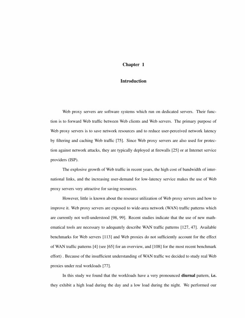
Web proxy servers are software systems which run on dedicated servers. Their func-
tion is to forward Web traffic between Web clients and Web servers. The primary purpose of
Web proxy servers is to save network resources and to reduce user-perceived network latency
by filtering and caching Web traffic [75]. Since Web proxy servers are also used for protec-
tion against network attacks, they are typically deployed at firewalls [25] or at Internet service
providers (ISP).
The explosive growth of Web traffic in recent years, the high cost of bandwidth of inter-
national links, and the increasing user-demand for low-latency service makes the use of Web
proxy servers very attractive for saving resources.
However, little is known about the resource utilization of Web proxy servers and how to
improve it. Web proxy servers are exposed to wide-area network (WAN) traffic patterns which
are currently not well-understood [98, 99]. Recent studies indicate that the use of new math-
ematical tools are necessary to adequately describe WAN traffic patterns [127, 47]. Available
benchmarks for Web servers [113] and Web proxies do not sufficiently account for the effect
of WAN traffic patterns [4] (see [65] for an overview, and [108] for the most recent benchmark
effort) . Because of the insufficient understanding of WAN traffic we decided to study real Web
proxies under real workloads [77].
In this study we found that the workloads have a very pronounced diurnal pattern, i.e.
they exhibit a high load during the day and a low load during the night. We performed our
2
study in an enterprise environment where Web proxy servers are deployed at the firewall of a
large internal corporate network. Later studies confirm the diurnal pattern at enterprise-level
Web traffic workloads [55, 109]. The difference between peak and off-peak load levels can be
an order of magnitude which leads to significant under-utilization of resource during off-peak
periods.
The use of real workloads in our study lead us to explore the opportunities that high
variance traffic patterns offer: This work develops and analyzes approaches that uses ex-
tra resources during off-peak periods to reduce resource utilization and user-perceived
network latency during peak periods.
The study also shows that network and disk I/O latencies have a significant influence on
Web proxy server performance. We found that memory and CPU utilization correlates more
with the number of open connections within a Web proxy server than with the request rate
[77]. If network latencies are low or the cache hit rate high, requests are completed quickly
and memory and CPU utilization is low even at peak workloads. This confirms our conjecture
that benchmarks which do not accurately model WAN latencies do not adequately measure Web
proxy server performance. Furthermore, we found that Web caching in the environment under
study actually slows down fast Internet responses. Also, the CPU and memory utilization of
Web proxy servers with caches more strongly correlates with workload than the utilization of the
same Web proxy servers without caches. These findings indicate that disk I/O is a performance
bottleneck. Later studies confirm this result [4, 109].
A surprising result of our study in [77] is that a Web proxy server architecture (CERN)
that relies heavily on file system services exhibited similar disk I/O as a Web proxy server
architecture (SQUID) which keeps meta-data in primary memory to avoid disk I/O. The results
of our subsequent study in [78] indicate that CERN’s access to the file system translates the
good locality of Web traffic [23, 104], into good buffer cache performance while SQUID does
not. In the same study we also show that by adjusting the Web proxy server interaction with a
standard Unix file system we achieve a reduction of disk I/O by 50% to 70%. We achieve even
3
further reductions of disk I/O by cache compaction during off-peak periods [78].
Resources are frequently purchased or leased in quanta of capacity, e.g. a T1 line, a disk
drive, or server hardware. For a network to perform well (i.e. low user-perceived latency), the
purchased resources need to match the peak traffic levels. Diurnal traffic patterns with high
variations therefore imply that a significant amount of resources are under-utilized during off-
peak periods and can be used at no extra cost. Past research on how to utilize idle times in
computer systems (see [54] for an overview) deals primarily with the discovery and utilization
of idle times in the scale from miliseconds to minutes.
In [79] we present an approach we call “bandwidth smoothing” that uses the extra band-
width capacity during the nightly off-peak periods of enterprise-level Web traffic to prefetch
Web content in order to increase the cache hit rate during peak periods. Other work in Web
prefetching attempt to improve performance over a smaller time window and accepts an in-
crease of bandwidth cost to reduce latency [70, 16, 14, 80, 27, 57]. We use machine learning
techniques to automatically generate prefetching strategies on a daily basis. This makes this
approach highly adaptable to Web traffic changes. The prefetching strategies perform with
high accuracy and medium coverage. Machine learning has been successfully applied in other
research areas such as branch prediction in computer architecture [21].
After providing the background for this work in Chapter 2 we study the resource uti-
lization of Web proxy servers under real workloads (Chapter 3). In Chapter 4 we evaluate
approaches to reduce disk I/O by adjusting Web proxy server interaction with a standard Unix
file system. In Chapter 5 we explore strategies to further reduce disk I/O using cache com-
paction during off-peak periods. Chapter 6 shows the potential of bandwidth smoothing and
introduces a mathematical model for evaluating the prefetch potential for any given bandwidth
profile. In Chapter 7 we evaluate automatically learned prefetch strategies using machine learn-
ing techniques. We conclude this work with Chapter 8.

Chapter 2
Background and Related Work
2.1 Web Proxy Servers
The function of a Web proxy is to relay a request in the form of a Uniform Resource
Locator (URL)[30] from a client to a server, receive the response of a server and send it back to
the client. If the proxy is configured to have a disk or memory cache, the proxy tries to serve a
client’s request out of its cache and only contacts the server in the case of a cache miss. A cache
miss occurs when the object is not in the cache or it has expired. When the request is relayed to
a server, the proxy translates the server name contained in the URL into an IP address in order
to establish a connection. This usually requires a query to the Domain Name Service (DNS)
[84, 85], which is typically implemented on a separate host on the same network as the proxy
to service all external mappings of host name to IP address for the enterprise.
2.1.1 Common Architectures
Most of the wallclock time of processing a single request is spent on waiting for I/O
to complete. For an enterprise-level Web proxy server with tens or hundreds of requests per
second it is therefore infeasible to process requests sequentially. There are multiple ways to
parallelize a Web proxy server (see [75] for a more detailed overview):
Process Forking The easiest way to parallelize request processing is to fork one process per
request and let the process terminate once the request is processed. Forking a process
5
for each request however introduces CPU overhead due to the fork system call. It
is now widely considered to be an inefficient solution [24, 83]. We found evidence
that the efficiency of this architecture seems to mainly depend on the efficiency of the
operating system’s process management [77]. Each process also replicates its own
name space which increases memory overhead and makes it more difficult to share
global information among processes. The advantage of this architecture is that Process
Forking is very robust: an error within one process does not affect any other processes.
A well known implementation of this architecture is CERN’s httpd [76] which was
the first available Web cache.
Process Mobs Another way to alleviate the forking overhead is to pre-fork a sufficiently large
number of processes and then delegate requests to them. A disadvantage is that long-
running processes might aggravate memory leaks, making this architecture less robust.
Existing Web proxy servers with this architecture often periodically restart processes
within the “mob” where the restart frequency is much lower than the arrival rate of
requests. Commercial Web caches such as Netscape’s Proxy Server seem to favor the
pre-forked architecture [75, 31]. A non-commercial implementation of this architec-
ture is “Jigsaw” which serves as a reference implementation of HTTP servers for the
World-Wide Web Consortium [8]. Jigsaw is designed as an experimental platform and
geared towards extensibility instead of high performance.
Multithreaded Both of the above architectures can be implemented by using multiple threads
instead of processes. This reduces the cost of context switching and reduces the state
size because all threads share the same address space. But because of this shared ad-
dress space, the code becomes harder to maintain. This architecture can also be com-
bined with multiprocess architectures where multiple threads are used where context
switching overhead would be high otherwise and multiple processes where the sepa-
ration of address spaces simplifies code maintenance. High end Netscape Web proxy
6
servers [75] use this architecture in combination with the process mob architecture.
Single Process, Asynchronous I/O This architecture avoids context switching overhead alto-
gether. It is an event-based architecture that is built around an event-loop. Web requests
are processed until the next potentially blocking I/O request. Each I/O request is reg-
istered at the event-loop and processing resumes whenever one of the registered I/O
requests become ready. The disadvantage of this architecture is the vulnerability due
to memory-leaks and the fact that processing of one request is not insulated from pro-
cessing of other requests. One error in the processing of one request can affect the
operation of the entire Web proxy server. SQUID which is currently the most pop-
ular non-commercial Web cache uses this architecture [123]. Because the design of
Squid is intended to ensure high performance and portability it bypasses some com-
mon operating system services by implementing its own virtual memory management
and scheduling. Beside the many advantages of portability it has the disadvantage of
not being able to take advantage of innovations in various operating systems as they
mature in a high traffic network environment [77]. Network Appliance’s Netcache is a
commercial Web proxy server based on this architecture [36]. Inktomi’s traffic server
[63] uses a combination of a multi-threaded and event-based architecture where threads
service an event loop.
In the following sections we will examine the architectures of two existing Web proxy
servers which will serve as reference for the rest of this paper. We chose these two architectures
because we found that their architectural differences combined with differences in performance
illuminates a number of general performance issues of Web proxy servers (see Chapter 3).
2.1.2 CERN
The first Web server was developed at the European Laboratory of Particle Physics
(CERN) and is called httpd for “HTTP daemon” [76]. httpd can also be used as a Web
7
proxy server. For the rest of this paper we will refer to the httpd operating in proxy mode as
CERN.
The CERN proxy forks a new process to handle each request. In caching configurations
CERN uses the file system to cache both data (Web objects) and proxy meta-data (expiration
times, content type). It translates the request into an object file name which it derives from the
structure of the URL: each URL component is translated into a directory name. The resulting
file name is a path through one or more directories. Thus, the length of the path depends on the
number of URL components. We call this path without the last component the URL directory.
The names of objects and their expiration dates are stored in a separate “meta-data file”
for each URL directory. To find out whether a request can be served from the cache, CERN
tries to open the meta-data file in the URL directory. Every component of the URL directory
name needs to be resolved. If the meta-data file exists and it lists the object file name as not
expired, CERN serves the request from the cache. In any other case, CERN relays the request to
the appropriate server and passes the server’s response to the client and stores it in its cache.
In a cacheless configuration, CERN only relays requests to server and passes responses
to clients. Processes are created to serve a single request after which they terminate. Objects
are removed from the cache by a separate “garbage collection” process that checks for expired
objects and deletes them.
2.1.3 SQUID
The SQUID proxy is the public domain network object cache portion [24] of the Har-
vest system [18]. The architecture was designed to be portable and to overcome performance
weaknesses of CERN: It uses its own non-blocking network I/O abstractions built on top of
widely available system calls and it avoids forking new processes except for relaying FTP re-
quests. “For efficiency and portability across UNIX-like platforms, the cache implements its
own non-blocking disk and network I/O abstractions directly atop a BSD select loop” (section
2.8 in [24]).

8
In managing its own resources, SQUID attempts to isolate itself from the operating sys-
tem. SQUID keeps meta-data about the cache contents in main memory. This enables SQUID to
determine whether it can serve a given request from its cache without accessing the disk. It also
maintains its own memory pools to reduce memory allocation and deallocation overhead.
SQUID maps URLs to files that are stored in a balanced directory tree. The balancing
of this tree is achieved by storing each successive miss in a different directory using a round-
robin scheme. The directories are created at start-up time and the number of directories is
configurable.
The cache has a LRU expiration policy which is activated once the cache size reaches
a configurable high mark, and deactivated once the cache size falls below a configurable low
mark. SQUID also uses main memory to cache objects that are currently in transit, to cache the
most recently used objects in a hot cache, and to cache error responses which resulted from bad
requests. In-transit objects have priority over error responses and hot cache objects.
SQUID implements its own DNS cache and uses a configurable number of “dns server”
processes to which it can dispatch non-blocking DNS requests.
The choice of this architecture has some interesting consequences:
• Each connection from a client and each connection to a server is represented as a
file descriptor. This means that a potentially large number of file descriptors must be
managed by a single process. This has repercussions on the overhead of system calls
• Operating system facilities such as the management of physical memory and file sys-
tem functionalities are replicated within the proxy
• Storing the meta-data for each cached object in memory means that main memory
utilization grows with the number of objects cached or the proxy cache size. Increasing
the cache size requires increasing both disk and main memory.
9
2.2 Web Caching
Web proxy servers are almost always configured to cache Web objects. Cceres et al. dis-
tinguish between data caching and connection caching. Data caching is the process of storing
requested objects on disk in the hope that subsequent requests will reference this object so that
it can be served locally instead of fetching it across the Internet. Connection caching reuses
connections between clients and the proxy server and the proxy server and the origin servers
(i.e. Web server which are the origin of Web objects). As we will describe in section 2.3.1 the
HTTP protocol requires a new connection for a request and a connection termination after the
response. Cceres et al. found that connection caching has a greater potential for saving latency
than data caching.
In most cases Web caching saves bandwidth and latency. Cceres et al. found that in
cases where the client/proxy connection is slow and the proxy/server connection is fast, a Web
cache can increase the bandwidth usage depending on how often clients abort requests. Proxy
server decouple the slow client connection from the fast server connection. This allows the
origin server to serve data much faster than if the server were directly connected to the client.
Thus, more bandwidth is used during the time period between client request and client abort.
2.2.1 Cache Coherency
Cache coherency is mechanism on which copies of a Web object are kept up-to-date. We
call a (cached) copy of an object “stale”, “invalid”, or “expired” if the original object changed,
and the copy does not reflect these changes. The likelyhood that a copy is stale is called the
“stale rate”. The “staleness” is the time since a copy became stale. The “expiration time stamp”
is the point in time at which a copy is predicted to become stale.
Although Web objects are changed frequently most Web objects do not have an expira-
tion time stamp. The best guarantee of cache consistency is therefore a Web cache invalidation
protocol such as the one proposed in [121]. In such a scheme Web servers keep track of objects
10
they served to caches. If an object at a server changes, the server notifies all caches that have
a copy of this object in order to invalidate those copies. Cache invalidation protocols require
extra communication overhead.
In [58] Gwertzman and Seltzer compare invalidation protocols with static and age-based
“Time-to-live fields” (TTLs). TTLs are an a priori estimate of an object’s life time that are
used to determine how long cached data remain valid. The challenge in supporting TTLs lies
in selecting the appropriate time out value. If a TTL is set for a too short interval the cache will
invalidate the object too soon and therefore reduce the hit rate. Setting a TTL for a too long
interval will increase the hit rate but also increase the likelyhood of serving stale objects. While
static TTLs carry fixed life times, age-based TTLs base life time predictions on the object’s age.
Based on trace-driven simulation Gwertzman and Seltzer show that age-based TTLs reduce
network bandwidth consumption by an order of magnitude and produces a stale rate of less than
5%. The simulated stale rate matches measurements reported by Glassman in [53] (he used
TTLs which equal 100% of the object’s age and found a stale rate of 8%). In the same study
Glassman also found that in the cases where the TTL was estimated too long, the time the page
actually changed was distributed roughly uniformly over the predicted TTL period. This means
that to reduce the stale data rate by half one had to reduce the TTLs by half and that, in turn,
would reduce the cache hit rate by half.
Krishnamurthy and Wills explore a technique they call “Piggyback Cache Validation”
(PCV) [68]. Instead of sending separate validation requests to servers, the cache piggybacks
a list of documents to be validated whenever it forwards requests to servers. According to
simulation results PCV reduces the proxy server communication while maintaining close-to-
strong cache coherency.
Dingle and Partl propose a number of improvements to the TTL cache consistency mech-
anism in [40]. One of these is to base age calculation of age-based TTLs not on the retrieval
time stamp of the object but on a time stamp at which it was last known to be non-stale. This
differentiation becomes necessary in cache meshes where both time stamps are equal only at
11
the origin server of the object. They furthermore advocate that users should be able to specify
a maximum staleness for each request. The HTTP 1.1 specification [48] incorporates the above
improvements.
As the Internet became more commercial a phenomena known as “cache busting” ap-
peared. Internet content providers rely increasingly on advertisement as main source of profit.
The evaluation of advertisement effectiveness is usually measured by the number of requests a
particular Web object receives (see [91, 100] for more information on this). The more requests
an object receives the more valuable it becomes as an advertisement site. Web caches are ex-
plicitly designed for reducing the number of requests at origin servers. With the proliferation
of Web caches Internet content providers started to make their Web objects uncacheable; for
example by setting the expiration date of an object to a time in the past and the last modifica-
tion date to a moment in the future. In the IETF Internet draft [87] propose a “hit metering”
protocol that specifies how caches can record request counts and report them back to servers. It
is still open whether the information demands of advertisers justify the introduction of an extra
protocol or whether other measures suffice that are either solely based on existing mechanisms
or on sampling and statistical methods [100].
2.2.2 Demand-driven Caching
Various researchers seem to agree that the maximum possible hit rate and byte hit rate
of demand-driven Web caching lies in between 30-50% [53, 1, 126, 6]. More recent studies
show that the hit rate is dependent on the proxy server’s client population size and the number
of requests seen by the proxy [23, 55, 42]. the maximal hit rates are around 50%. Depending
on network connectivity and disk I/O latencies the hit time can be orders of magnitude different
from the miss time. Thus a comparatively low Web cache hit rate can still achieve a significant
time improvement.
For caches of small size the cache replacement strategy is an important factor in de-
termining the hit rate. The most commonly implemented cache replacement strategy is Least
12
Recently Used (LRU) which removes cached objects with the least recent access time stamps.
As reported in [126] LRU is sub-optimal because it ignores the size of documents. Extending
LRU with sensitivity to size improves the hit rate. Arlitt found that a combination of Least
Frequently Used (LFU) and aging yields the best results [7]. Furthermore, their trace driven
simulations seem to indicate that thresholding policies and cache partitioning policies do not
appear to be effective. Recent publications propose caching strategies which account for the
relative retrieval latency of an object (i.e. the time to fetch an object from its server devided by
its size) [111, 129, 74].
With the decreasing cost of secondary storage devices it becomes practical to use “infinite
caches”, i.e. objects are removed from the cache not because of limited space but because of
their staleness. Thus, strategies to determine staleness become more influential on hit rate than
cache replacement algorithms [120, 90]. In section 2.2.4 we will discuss the benefit of caching
approaches which use primary memory only. The greater cost of primary memory limits the
cache size and increases the importance of replacement algorithms.
Once an “infinite cache” is available, two ways to improve Web caching remain: the hit
rate can be increased by prefetching and the overall service time can be reduced by shorter hit
times. In the following two sections we survey the literature on prefetching and disk I/O.
2.2.3 Prefetching
Prefetching can be used to achieve two complementary goals: the first one is to reduce
network latency as it is perceived by Web users by increasing hit rate, and the second goal is
to “smooth” bandwidth consumption such that more bandwidth is consumed during idle times
and less bandwidth is consumed during peak times (see Chapter 6 and 7 or [79]). In both cases
a prefetching mechanism attempts to anticipate future references to Web objects in order to be
able to serve them from a cache when they are actually needed.
The greatest challenge in prefetching is to achieve efficient prefetching. In [119] Wang
and Crowcroft define prefetching efficiency as the ratio of prefetch hit rate (the probability
13
of a correct prefetch) and the relative increase of bandwidth consumption to achieve that hit
rate. Assuming a simplifying queueing model (M/M/1) they show an exponential relationship
between the bandwidth utilization of the network link and the required prefetching efficiency to
ensure network latency reduction. Crovella and Barford propose “rate controlled prefetching”
in which traffic due to prefetching is treated as a lower priority than traffic due to actual client
requests [33].
Prefetching will never be able to reduce bandwidth consumption. But it can be used to
reduce the required bandwidth capacity of a network connection. In [32] Crovella and Barford
show that bandwidth smoothing can lead to an overall reduction of queueing delays in a network
and therefore to an improvement of network latency. We are not aware of any work (other
than ours) that investigates real Web traffic work loads in terms of shifting peak bandwidth
usage to off-peak periods through prefetching; Most work on prefetching focuses on short-term
prefetching to reduce interaction latency.
The overview given in [119] distinguishes two approaches of prefetching: server-initiated
and client-initiated prefetching. These approaches differ based on whether prefetching decisions
are inferred from data located at a Web server or at a Web client respectively. This data can be
either statistical or deterministic. Statistical data is usually based on access history and provides
conditional probabilities of object references given a certain set of references. Deterministic
data are prefetch instructions that are either defined by the content provider at the server side
or as user preferences at the client side. In [45] the authors distinguish three prefetching cate-
gories depending on where prefetching is applied: (1) between Web servers and browser clients;
(2) between Web servers and proxies; and (3) between proxies and browser clients. The work
mentioned so far belongs to the first category.
A server-initiated, client/server prefetching approach based on the structure of Web ob-
jects and user access heuristics as well as statistical data is presented in [118]. Padmanabhan
and Mogul present an evaluation of a server-initiated approach in which the server sends replies
to clients together with “hints” indicating which objects are likely to be referenced next [95].
14
Their trace-driven simulation showed that their technique could significantly reduce latency at
the cost of an increase in bandwidth consumption by a similar fraction. Padmanabhan and
Mogul’s approach is based on small extensions to the existing HTTP protocol. A similar study
but with an idealized protocol was performed by Bestavros [15, 14] in which the author pro-
poses “speculative service” in which a server sends replies to clients together with a number of
entire objects. This method achieved up to ca. 50% reduction in perceived network latency.
In [70] Kroeger et al. examine the potential latency reduction by applying prefetching
between servers and proxies. Their study is based on the same traces as our analysis in sec-
tion 6.2.3. They found that a combined caching and prefetching approach can at best reduce
latency by 60%. Furthermore, the potential latency reduction depends on how far in advance
an object can be prefetched. For prefetch lead times below 100 seconds, the latency reduc-
tion is significantly lower. In bandwidth smoothing we assume a diurnal bandwidth profile and
prefetch lead times of up to twelve hours. Markatos and Chronaki [80] propose that Web servers
regularly push their most popular documents to Web proxies, which then push those documents
to clients. Their results suggest that this technique can anticipate more than 40% of a client’s
requests. Similar techniques are explored by Cohen [27]. Wcol [62] is a proxy-initiated ap-
proach which parses HTML files and prefetches links and embedded images but does not push
the documents to clients. Gwertzman and Seltzer [57] propose a technique called “geographical
push-caching” where Web servers push Web objects to caches that are closest to its clients. The
technique assumes sufficiently accurate knowledge of network topology.
There are two commercial products available which use proxy/server prefetching tech-
nologies. CacheFlow, Inc. uses “Active Web Caching” in their Web proxy cache server which
keeps cached popular Web objects updated [20]. The CacheFlow product uses access history
information to determine the popularity of objects. SkyCache, Inc. addresses the problem that
the sample of individual caching sites might not be sufficient for good predictions [112]. Their
approach is to maintain large national caches and continually broadcast the most popular and
up-to-date content over a satellite link to Web caches at Internet service providers (ISPs). Popu-
15
larity is determined by collecting access statistics from each ISP cache. The advantage of using
satellite links for prefetching is that it avoids network congestion points and relieves traditional
links from high bandwidth prefetch traffic. Broadcasting content to ISP caches scales well and
simplifies keeping ISP caches up-to-date.
Client/proxy approaches also have the advantage that they do not increase the usually
expensive bandwidth on proxy/server links and that they have more information about client
behaviour. Loon and Bharghavan [73] present a design and implementation of a client-initiated,
client/proxy approach which performs prefetching, image filtering, and hoarding for mobile
clients. In [45] Fan et al. study a similar system and show that a combination of large caches at
Web clients and delta-compression can reduce user-perceived latency up to 23%. The authors
use the Prediction-by-Partial-Matching (PPM) algorithm whose accuracy ranges from 40% to
73% depending on its parameters. The authors also find that it is important that their predictor
observe all user accesses, including browser cache hits. Browser cache hits are not visible at
Web server proxies.
The PPM algorithm is inspired by a study by Krishnan and Vitter demonstrating the
relationship between data compression and prediction [117, 35]. Most file system studies about
cache-based approaches to file prefetching [56, 115, 97] use compressor-based predictors.
2.2.4 Web Cache Disk I/O
Apart from network latencies the bottleneck of Web cache performance is disk I/O
[4, 109, 124]. An easy but expensive solution would be to just keep the entire cache in pri-
mary memory. However, various studies have shown that the Web cache hit rate grows in a
logarithmic-like fashion with the amount of traffic and the size of the client population [55,
42, 23] as well as logarithmic-proportional to the cache size [5, 53, 23, 126, 55, 104, 34, 42]
(see [19] for a summary and possible explanation). In practice this results in cache sizes in the
order of ten to hundred gigabytes or more [116]. To install a server with this much primary
memory is in many cases still not feasible.
16
Addressing the disk I/O bottleneck in Web caching can be classified into three categories
depending on the technology used to interface with disk drives. The most promising but also
most expensive approach is to use a special purpose operating system. Commercial products
such as CacheFlow [20] and Network Appliance’s NetCache [36] use this approach. Related to
this approach are commercial products that use standard operating systems which are specifi-
cally tuned for the Web caching software and a hardware platform, e.g. Inktomi’s Traffic Server
[63] and Cobalt’s CacheQube [26].
A more portable solution is to build a special purpose file system which is tuned to Web
traffic. The Squid developer community is starting to build a “squidfs” [72]. This approach
allows to tune disk layout, disk access, and buffering to the specific needs of Web caching. Pai
et al. [96] propose a workload balancing approach for Web cache clusters which takes request
locality into account. The improvement of performance is due to a better utilization of standard
file system buffer caches.
Nishikawa et al. [89] suggests that main-memory-based caching architectures become
feasible if only frequently accessed objects are stored and distribution of content among clus-
tered main-memory-based caches is carefully tuned. Their results are based on a statistical
analysis of traces data and suggest that their strategies can reduce the necessary cache size by
orders of magnitude without affecting hit rate. Unfortunately, the authors do not specify the size
of source of their traces.
2.3 Web Proxy Server Traffic
The world-wide Web traffic is using a number of protocols, however by far the most traf-
fic is based on the Hypertext Transfer Protocol (HTTP) [121]. The following section considers
the performance of the HTTP protocol since it has implications to bandwidth consumption and
network latency and thus impacts Web cache performance. We then look at Web proxy traf-
fic characteristic and review recent findings about wide-area network traffic characteristics and
conclude with an overview of existing benchmarks which aim to simulate Web proxy server

17
traffic.
2.3.1 The HTTP protocol and its Performance
The HTTP protocol is layered over a reliable, connection oriented protocol, normally
TCP [101]. Each HTTP interaction consists of a request sent from the client to the server, fol-
lowed by a response sent from the server to the client. Requests and response are expressed in
a simple ASCII format. The precise specification of HTTP is in an evolving state. Most exist-
ing implementations are based on the HTTP 1.0 specification [11] (see also the informational
document [13]). Implementors of widely used HTTP applications are planning to soon release
versions which conform to the new HTTP 1.1 specification. HTTP 1.1 is currently a proposed
standard in the Internet Engineering Task Force (IETF) standardization process [48].
An HTTP request includes several elements: a Method such as GET or PUT or POST,
an object name and a set of Hypertext Request headers, with which a client specifies things
such as the kinds of documents it is willing to accept, authentication information, etc.; and
an optional data field, used with certain methods such as PUT. The server parses the request,
then takes action according of the specified method. It then sends a response to the client,
including a status code to indicate if the request succeeded, or a reason, why it didn’t succeed;
a set of object headers including meta-information about the object returned by the server and
optionally including the “content-length” of the response; and a Data field, containing the object
requested. Note that both requests and responses end with a data field of arbitrary length. The
HTTP protocol specifies three possible ways to indicate the end of the data field: (1) if the
“content-length” field is present, it indicates the size of the data field; (2) the “content-type”
field may specify a delimiter of a MIME multipart message [17]; and (3) the server (but not the
client) may indicate the end of the message simply by closing the TCP connection after the last
data byte.
In [94, 114] the authors identify a number of inefficiencies of the HTTP 1.0 protocol.
HTTP opens and closes a TCP connection for every single object which requires at least two
18
network round trips per object (one for opening the connection and one for requesting and trans-
mitting the data). This is exacerbated by Hypertext Markup Language (HTML) objects [12]
which typically include references to in-lined images which need to be requested separately
each. Other inefficiencies are caused by connection setup and tear-down processing overhead
and by TCP’s “TIME-WAIT” states. The latter is caused by the requirement of the TCP specifi-
cation to remember certain per-connection information for four minutes [101]. On a busy server
this can either lead to dropped connections or excessive connection table management costs. In
[3] the authors report a factor of two to nine increase of service times because of connections in
“TIME-WAIT” states.
Improvements of the HTTP 1.0 protocol come from the HTTP 1.1 protocol specification
[48] which most importantly introduces persistent connections. This allows a client to issue
multiple requests and receive multiple responses over a single connection. This leads to less
connection setup and tear-down overhead, fewer round-trips and more efficient use of TCP
packets because of buffering. There are also investigations into more efficient HTTP carrier
protocols [59].
2.3.2 Wide-Area Network Traffic
Analytical models of computer systems are commonly based on Queueing Theory [66,
67]. These models have been proven to be quite accurate in their predictions and much easier
to construct and evaluate than simulations [64]. These models commonly assume that arrival
of requests are independent from each other, i.e. the arrival process follows a Poisson pro-
cess. Paxson and Floyd [99, 98] show that wide-area network (WAN) arrival processes clearly
does not follow a Poisson model and that the inter-arrival times have heavy-tailed distributions
suggesting long-term dependencies. This has far-reaching implications for the performance
analysis of systems which are exposed to WAN traffic. Since these heavy-tailed distributions
often have infinite means, well-known analytical tools based on Mean-Value Analysis (MVA)
[71, 106, 128] become meaningless. Recent work by Feldmann et al. [47] suggest that WAN
19
traffic can be robustly modeled by multifractal processes (see for example [44, 61]). To our
knowledge the equivalent of queueing theory for WANs does not exist, yet. Finding the appro-
priate mathematical tools is still on-going research.
2.3.3 Web Proxy Server Traffic
The above results make quantitative predictions of Web proxy server performance dif-
ficult. Current work on Web proxy server traffic characterization is motivated by a best-effort
approach and has focussed on traffic characterizations which aid the design of Web proxy server
components that are believed to have potential for improving performance. One such com-
ponent is Web caching. Breslau et al. [19] summarize the research on Web cache centered
characterization of Web proxy server traffic and mathematically reduce commonly observed
phenomena to one common observation which states that the popularity of Web objects follows
a Zipf-like distribution Ω/iα very well (where Ω = (∑N
i=1 1/iα)−1 and i is the ith most popular
Web object). The α values range from 0.64 to 0.83. Traces with homogenous communities have
a larger α value than traces with more diverse communities. The traces generally do not follow
Zipf’s law which states that α = 1 [130]. The authors show that this implies the following
commonly observed properties:
• The Web cache hit rate grows in a logarithmic-like fashion with the amount of traffic
and the size of the client population [55, 42, 23]
• The hit rate grows in a logarithmic-like fashion with the cache size [5, 53, 23, 126, 55,
104, 34, 42]
• The traffic exhibits excellent temporal locality: the probability that a document will be
referenced k times after it was last referenced tends to be proportional to 1/k [104, 23].
There is low correlation between the popularity of an object and its size, even though the
average size of unpopular objects is larger than the average size of popular objects (see Chapter 4

20
and [22, 78]). The more popular an HTTP object is, the more likely it stays a popular object.
The day-to-day membership variation of the top 1% most popular objects is much lower than
the variation in the top 10% most popular objects (see Chapter 6 and [22, 79]). This allows for
relatively static working set capture algorithms as is demonstrated by Rousskov et al. [110]. In
a study which explores rate of change, age, and inter-modification time of Web objects, Douglis
et al. [41] find that 22% of the resources referenced in their traces are accessed more than once,
but about half of all references were to those 22%. Of this half, 13% were to a resource that had
been modified since the previous traced reference to it. The same study also finds that content
type and rate of access have a strong influence on rate of change, age, and inter-modification
time, the domain has a moderate influence, and size has little effect.
Feldmann et al. [46] demonstrate that the analysis of low-level packet traces of HTTP
traffic reveal a number of new Web proxy server performance issues. In particular the authors
distinguish between environment with mismatching bandwidths, i.e. slow client/proxy link
but fast proxy/server link, and high-bandwidth-only environments. According to their trace-
driven simulation, the latency reduction due to caching in an environment with mismatching
bandwidths is only 8% and the bandwidth might even increase due to aborted connections. Their
results suggest that caching connections instead of data could reduce the latency by 25%. In a
high-bandwidth environment, data cache improves latency by 38%, connection cache improves
it by 35%, and the combination of the two improves it by 65%.
2.4 Machine Learning
Machine-learning methods are appropriate whenever hand-engineering of software is
difficult and yet data is available for analysis by learning algorithms. Web caches continually
produce access data of rapidly growing traffic with frequently changing characteristics. Hence
it becomes necessary to frequently adapt a Web caching task that requires traffic analysis to new
traffic patterns.
Learning tasks that the Machine Learning research area considers can generally be di-
21
vided into one-shot decision tasks (classification, prediction) and sequential decision tasks (con-
trol, optimization, planning). One-shot decision tasks are usually formulated as supervised
learning tasks, where the learning algorithm is given a set of input-output pairs (labeled data).
The input describes the information available for making the decision and the output describes
the correct decision [38].
Sequential decision tasks are usually formulated as reinforcement learning tasks, where
the learning algorithm is part of an agent that interacts with an “external environment.” At
each point, the agent observes the current state of the environment (or some aspects of the
environment). It then selects and executes some action, which usually causes the environment
to change state. The environment then provides some feedback (e.g., immediate reward) to the
agent. The goal of the learning process is to learn an action-selection policy that will maximize
the long-term rewards received by the agent [38] (see [49] for an overview).
Because we are interested in the automatic analysis of labeled data based on Web cache
traces we will focus on supervised learning tasks.
The result of a learning task is a classification model which allows the classification of
unseen data below a certain error rate. There are a multiple classification formalisms avail-
able: inductive classification, instance-based classifiers, neural networks, genetic algorithms,
and statistical nearest-neighbor methods (see [102] for a short overview of these methods). In
the following sections we will focus on inductive classification.
The result of inductive classification are decision trees which have the advantage that
they classify data very efficiently once they are created. This is due to the fact that they directly
map to the “if-then-else” program language construct. Decision trees can become very large
and difficult to understand. There are various approaches to make decision trees more readable
to humans. In [102] Quinlan derives production rules from decision trees, a format that appears
to be more intelligible than trees.
The approach that we intend to use in Chapter 7 is implemented as a publicly available
tool called RIPPER [29] which produces and evaluates production rule sets on labeled training

22
and test data.
2.5 Summary
We introduced the common architectures of Web proxy servers and presented the two
reference Web proxy servers of this paper in more detail. While the functionality of Web proxy
servers is very simple, the fact that it is necessary to process many requests in parallel without
incurring much latency, makes the choice of architectural features a non-trivial task. As we will
see in Chapter 3 some of the performance impacts of the above architecture are not obvious.
We also surveyed the research literature on HTTP performance, Web traffic, Web cache
caching strategies and prefetching, Web cache consistency, and machine learning.
Chapter 3
Resource Utilization of Web Proxy Servers
3.1 Introduction
In this Chapter we will analyze the resource utilization of CERN and SQUID under real
workloads. This includes the memory, CPU, and disk utilization. The comparison of CERN
and SQUID is interesting because CERN’s architecture is simple and relies heavily on standard
operating system services, while SQUID duplicates many operating system services in order
to have more control over them. By closely studying the resource utilization of these two
architectures we gain better understanding of the interaction of web proxy servers with operating
system which in turn prompts ways to improve web proxy server performance.
3.2 Methodology
3.2.1 Workload
Our workload is taken from the web traffic at Digital Equipment Corporation’s (Digital)
Palo Alto Gateway which has a web proxy located at and managed by the Network Systems Lab
at Palo Alto, CA. The gateway relays web communication between much of Digital’s intranet
and the Internet. A large fraction of the North American and Asian sites use this gateway. A
measurement infrastructure allows us to collect system and application performance data on a
daily basis in a fully automated fashion. We have collected almost a year’s worth of data during
24
the deployment of various commercial and non-commercial web proxies1.
Real world workloads are by definition not repeatable, and contain a multitude of errors.
The chosen workload samples strive to represent best case workload patterns because it is easier
to find comparable best workloads than comparable failure modes. For the analysis presented
in this paper we decided to select workloads based on the following criteria:
• The load occurred during a business day. We are interested in high load testing -
business days exhibit a two to three time higher load than weekends.
• The proxy under test delivers 24 hours of uninterrupted service. This was a surprisingly
limiting criterion: the proxies were unreliable especially in a caching configurations.
• Little detectable anomalous network behavior. We used the the length of the system
network tcp queue for pending connections to the Internet (SYN SENT queue) and the
access level for indicators of network problems. Unusually large SYN SENT queues
or unusually low access levels are generally caused by Internet service failures.
• The Domain Name Service (DNS) average service time is reasonably short for the en-
tire 24 hour period. Occasionally, the DNS degenerates, which increases proxy service
time and skews our measurements.
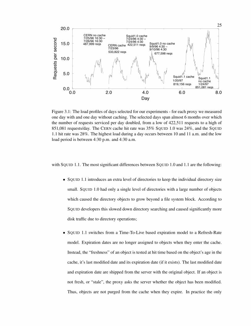
Selecting workloads based on the above criteria results in a selection which represents
best cases instead of average cases. The curves of the selected workloads are shown in fig-
ure 3.1. Each workload is taken from a 24 hour time period. The selected workloads are from
days which span almost six months over which the number of daily requests almost doubled.
3.2.2 SQUID versions
At the time we started our experiments SQUID 1.0 was the most recent version available.
Half a year later SQUID seemed to have matured significantly and we repeated the experiments1 Colleagues have collected proxy request traces that are now available for public use [69]. The current traces
contain data taken between 29 August 1996 and 22 September 1996. This is a total of 24,477,674 references.
25
0.0 2.0 4.0 6.0 8.0Day
0.0
5.0
10.0
15.0
20.0
Requ
ests
per
sec
ond
CERN no cache7/25/96 16:30 −7/26/96 16:30
CERN cache7/23/96
Squid1.0 cache7/23/96 4:30 −7/24/96 4:30 Squid1.0 no cache
9/9/96 4:30 −9/10/96 4:30
Squid1.1 cache Squid1.1no cache1/24/97
1/20/97
487,999 reqs
533,822 reqs
422,511 reqs
677,598 reqs
819,156 reqs851,081 reqs
Figure 3.1: The load profiles of days selected for our experiments - for each proxy we measuredone day with and one day without caching. The selected days span almost 6 months over whichthe number of requests serviced per day doubled, from a low of 422,511 requests to a high of851,081 requests/day. The CERN cache hit rate was 35% SQUID 1.0 was 24%, and the SQUID1.1 hit rate was 28%. The highest load during a day occurs between 10 and 11 a.m. and the lowload period is between 4:30 p.m. and 4:30 a.m.
with SQUID 1.1. The most significant differences between SQUID 1.0 and 1.1 are the following:
• SQUID 1.1 introduces an extra level of directories to keep the individual directory size
small. SQUID 1.0 had only a single level of directories with a large number of objects
which caused the directory objects to grow beyond a file system block. According to
SQUID developers this slowed down directory searching and caused significantly more
disk traffic due to directory operations;
• SQUID 1.1 switches from a Time-To-Live based expiration model to a Refresh-Rate
model. Expiration dates are no longer assigned to objects when they enter the cache.
Instead, the “freshness” of an object is tested at hit time based on the object’s age in the
cache, it’s last modified date and its expiration date (if it exists). The last modified date
and expiration date are shipped from the server with the original object. If an object is
not fresh, or “stale”, the proxy asks the server whether the object has been modified.
Thus, objects are not purged from the cache when they expire. In practice the only
26
difference between the two schemes is that the Refresh-Rate model keeps objects after
they have expired and is able to use the object if the server reports that the object has
not been modified.
3.2.3 Measurement Framework
The proxy experiments used two dedicated Digital Alpha Station 250 4/266 machines
with 512 MB of main memory and 8 GB of proxy cache disk space. DNS round-robin split
the load between the two to insure that each had more than sufficient hardware resources. An
additional process logged system statistics every 15 minutes; once a day all logs were shipped
to other machines for log processing and archiving.
A set of standard Unix tools ran every 15 minutes to measure proxy resource consump-
tion. Among other things, these tools provided information about the CPU idle time (iostat), the
memory allocated by processes (ps) and by the network (netstat), and the total number of disk
accesses per second (iostat). Each of these measurements are snapshots and do not summarize
the activity of the whole 15 minutes.
This sampling approach allows us to continuously monitor the overall system behavior,
collecting data for months on end. From this we know the baseline performance of the system,
the expected load for a given day and time, and have the ability to detect network problems
that are unrelated to the proxy yet affect its performance or the service seen by the clients. By
monitoring the length of the tcp (SYN SENT queue) we can detect quality of service failures
to portions of the Internet. Monitoring the length of the tcp (SYN RCVD queue) we can detect
failures on the corporate Intranet.
Snapshot measures provide an accurate measure of system behavior at a single point
in time; this preserves details that might be lost when aggregating the performance over large
periods of time. Collecting sufficient samples over long periods of time produces a full range of
expected behavior and errors. The drawback of this technique is that it is not possible to tightly
correlate events. This would be difficult even with precisely correlated measurements because

27
proxy service is a pipeline within which arbitrary delay and queueing occur. Thus, the request
rate is decoupled from the serviced request rate.
The regular logs of CERN and SQUID did not give us precise information about the
duration of the proxy service times. To obtain more accurate data we instrumented CERN and
SQUID 1.0. The service time duration is the time from receiving a request from a client to
terminating the connection to a client, effectively the time that the end user waits for a request
to be completed. We summarize the service time durations and the number of requests serviced
per second (rps) every 15 minutes taking the mean and distribution of all measurement points.
3.3 Results
Two different configurations were evaluated for each of the three proxies: a proxy with-
out cache and a proxy with 8 GB disk space for caching. For the caching configurations we set
the time-to-live or refresh-rate to 50% of the time since last modification.
For cache configurations the performance is also dependent on cache hit rate. CERN’s
hit rate was 35%, SQUID 1.0 was 24%, and SQUID 1.1 had a hit rate of 28%. Different hit rates
have an impact on average service times and resource utilization. We will discuss these hit rate
differences in section 3.3.2.
3.3.1 Resource Requirements
CPU utilization
Proxy CPU requirements determine the basic load that a workstation or server can han-
dle. If the CPU requirements scale linearly with load, then CPU load characterization can
establish server requirements for expected workloads. Understanding the components of the
CPU requirements allow one to predict the CPU requirements on other systems or other config-
urations.
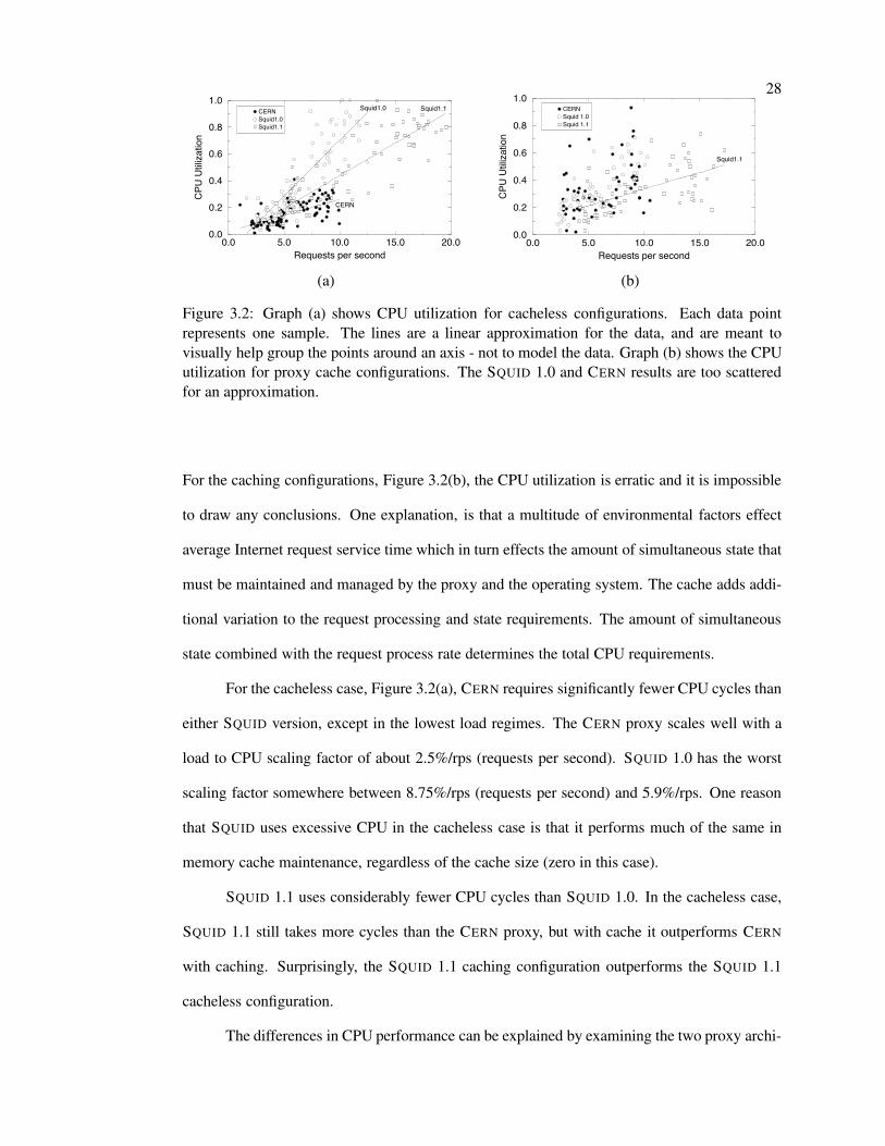
The CPU utilization of CERN and SQUID are shown in Figure 3.2. The CPU usage is
not as tightly correlated with the workload request per second service rate as one would hope.
28
0.0 5.0 10.0 15.0 20.0Requests per second
0.0
0.2
0.4
0.6
0.8
1.0
CPU
Utiliz
atio
n
CERNSquid1.0Squid1.1
Squid1.0 Squid1.1
CERN
0.0 5.0 10.0 15.0 20.0Requests per second
0.0
0.2
0.4
0.6
0.8
1.0
CPU
Utiliz
atio
n
CERNSquid 1.0Squid 1.1
Squid1.1
(a) (b)
Figure 3.2: Graph (a) shows CPU utilization for cacheless configurations. Each data pointrepresents one sample. The lines are a linear approximation for the data, and are meant tovisually help group the points around an axis - not to model the data. Graph (b) shows the CPUutilization for proxy cache configurations. The SQUID 1.0 and CERN results are too scatteredfor an approximation.
For the caching configurations, Figure 3.2(b), the CPU utilization is erratic and it is impossible
to draw any conclusions. One explanation, is that a multitude of environmental factors effect
average Internet request service time which in turn effects the amount of simultaneous state that
must be maintained and managed by the proxy and the operating system. The cache adds addi-
tional variation to the request processing and state requirements. The amount of simultaneous
state combined with the request process rate determines the total CPU requirements.
For the cacheless case, Figure 3.2(a), CERN requires significantly fewer CPU cycles than
either SQUID version, except in the lowest load regimes. The CERN proxy scales well with a
load to CPU scaling factor of about 2.5%/rps (requests per second). SQUID 1.0 has the worst
scaling factor somewhere between 8.75%/rps (requests per second) and 5.9%/rps. One reason
that SQUID uses excessive CPU in the cacheless case is that it performs much of the same in
memory cache maintenance, regardless of the cache size (zero in this case).
SQUID 1.1 uses considerably fewer CPU cycles than SQUID 1.0. In the cacheless case,
SQUID 1.1 still takes more cycles than the CERN proxy, but with cache it outperforms CERN
with caching. Surprisingly, the SQUID 1.1 caching configuration outperforms the SQUID 1.1
cacheless configuration.
The differences in CPU performance can be explained by examining the two proxy archi-
29
tectures and the system cost of various operations which all proxies rely on heavily. CERN forks
a new process for each request, and keeps no meta-data or state internally in the process (the
cache is implemented entirely on disk). Each process has very little state to scan or to pass into
the kernel for network related system calls. Forking a process for each request incurs a large
overhead which is eliminated in the SQUID architecture. The SQUID architecture eliminates
process forking; it implements asynchronous I/O within a single thread and stores all the cache
meta-data in main memory in order to improve cache response time. This results in additional
CPU cycles to manage all the network connections in a single process, to process much more
state for network system calls, and to manage the in-memory meta-data.
With the Digital Continuous Profiling Infrastructure (DCPI2) [10] we compared the CPU
usage profile of CERN and SQUID 1.1. For the DCPI results, we collected two sets of samples,
of 20 minutes for each configuration. The two cacheless configurations were run in parallel,
and the two cached configurations were run in parallel. This eliminates differences in external
network behavior between the samples. Prior to the final DCPI run, many other samples were
taken; the cycles/request varied somewhat but the conclusions were consistent reguardless of
load or time of day. Furthermore, these results are consistent with the measurements shown in
Figure 3.2 and with the related work in [3]. The latter demonstrates that a vast majority of the
CPU time is spent in kernel routines and implies that a proxy’s major function is to manage
network connections and pass data.
Table 3.1 shows the profiling results normalized to the number of cycles required to
process a request (cpr) (kernel idle cycles were filtered out). The most obvious result is that the
native proxy executes only 12% – 18% of the cycles required to process a request. CERN relies
directly on the kernel to manage resources while SQUID manages many of its own resources via2 DCPI: The Digital Continuous Profiling Infrastructure for Digital Alpha platforms permits continuous low-
overhead profiling of entire systems, including the kernel, user programs, drivers, and shared libraries. The systemis efficient enough that it can be left running all the time, allowing it to be used to drive on-line profile-basedoptimizations for production systems. The Continuous Profiling Infrastructure maintains a database of profile infor-mation that is incrementally updated for every executable image that runs. A suite of profile analysis tools analyzesthe profile information at various levels. The tools used for this analysis show the fraction of cpu cycles spentexecuting the kernel and each user program procedure.
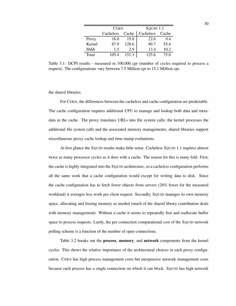
30CERN SQUID 1.1
Cacheless Cache Cacheless CacheProxy 16.0 19.8 22.6 9.4Kernel 87.9 128.6 89.7 55.4Shlib 1.5 2.9 13.4 10.2Total 105.4 151.3 125.6 75.0
Table 3.1: DCPI results - measured in 100,000 cpr (number of cycles required to process arequest). The configurations vary between 7.5 Million cpr to 15.1 Million cpr.
the shared libraries.
For CERN, the differences between the cacheless and cache configuration are predictable.
The cache configuration requires additional CPU to manage and lookup both data and meta-
data in the cache. The proxy translates URLs into file system calls; the kernel processes the
additional file system calls and the associated memory managements; shared libraries support
miscellaneous proxy cache lookup and time-stamp evaluations.
At first glance the SQUID results make little sense. Cacheless SQUID 1.1 requires almost
twice as many processor cycles as it does with a cache. The reason for this is many fold. First,
the cache is highly integrated into the SQUID architecture, so a cacheless configuration performs
all the same work that a cache configuration would except for writing data to disk. Since
the cache configuration has to fetch fewer objects from servers (28% fewer for the measured
workload) it averages less work per client request. Secondly, SQUID manages its own memory
space, allocating and freeing memory as needed (much of the shared library contribution deals
with memory management). Without a cache it seems to repeatedly free and reallocate buffer
space to process requests. Lastly, the per connection computational cost of the SQUID network
polling scheme is a function of the number of open connections.
Table 3.2 breaks out the process, memory, and network components from the kernel
cycles. This shows the relative importance of the architectural choices in each proxy configu-
ration. CERN has high process management costs but inexpensive network management costs
because each process has a single connection on which it can block. SQUID has high network
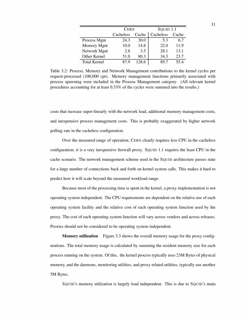
31CERN SQUID 1.1
Cacheless Cache Cacheless CacheProcess Mgnt 24.3 30.0 5.3 6.7Memory Mgnt 10.0 14.8 22.0 11.9Network Mgnt 2.6 3.5 28.1 13.1Other Kernel 51.0 80.3 34.3 23.7Total Kernel 87.9 128.6 89.7 55.4
Table 3.2: Process, Memory and Network Management contributions to the kernel cycles perrequest-processed (100,000 cpr). Memory management functions primarily associated withprocess spawning were included in the Process Management category. (All relevant kernelprocedures accounting for at least 0.33% of the cycles were summed into the results.)
costs that increase super-linearly with the network load, additional memory management costs,
and inexpensive process management costs. This is probably exaggerated by higher network
polling rate in the cacheless configuration.
Over the measured range of operation, CERN clearly requires less CPU in the cacheless
configuration; it is a very inexpensive firewall proxy. SQUID 1.1 requires the least CPU in the
cache scenario. The network management scheme used in the SQUID architecture passes state
for a large number of connections back and forth on kernel system calls. This makes it hard to
predict how it will scale beyond the measured workload range.
Because most of the processing time is spent in the kernel, a proxy implementation is not
operating system independent. The CPU requirements are dependent on the relative use of each
operating system facility and the relative cost of each operating system function used by the
proxy. The cost of each operating system function will vary across vendors and across releases.
Proxies should not be considered to be operating system independent.
Memory utilization Figure 3.3 shows the overall memory usage for the proxy config-
urations. The total memory usage is calculated by summing the resident memory size for each
process running on the system. Of this, the kernel process typically uses 23M Bytes of physical
memory, and the daemons, monitoring utilities, and proxy related utilities, typically use another
5M Bytes.
SQUID’s memory utilization is largely load independent. This is due to SQUID’s main
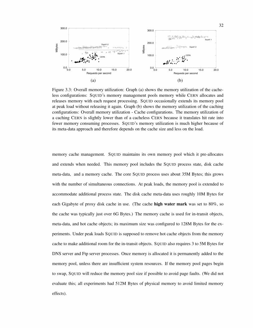
32
0.0 5.0 10.0 15.0 20.0Requests per second
0.0
100.0
200.0
300.0
MBy
tes
CERN
Squid1.0
Squid1.1
0.0 5.0 10.0 15.0 20.0Requests per second
0.0
100.0
200.0
300.0
MBy
tes
Squid1.1
Squid1.0
CERN
(a) (b)
Figure 3.3: Overall memory utilization: Graph (a) shows the memory utilization of the cache-less configurations: SQUID’s memory management pools memory while CERN allocates andreleases memory with each request processing. SQUID occasionally extends its memory poolat peak load without releasing it again. Graph (b) shows the memory utilization of the cachingconfigurations: Overall memory utilization - Cache configurations. The memory utilization ofa caching CERN is slightly lower than of a cacheless CERN because it translates hit rate intofewer memory consuming processes. SQUID’s memory utilization is much higher because ofits meta-data approach and therefore depends on the cache size and less on the load.
memory cache management. SQUID maintains its own memory pool which it pre-allocates
and extends when needed. This memory pool includes the SQUID process state, disk cache
meta-data, and a memory cache. The core SQUID process uses about 35M Bytes; this grows
with the number of simultaneous connections. At peak loads, the memory pool is extended to
accommodate additional process state. The disk cache meta-data uses roughly 10M Bytes for
each Gigabyte of proxy disk cache in use. (The cache high water mark was set to 80%, so
the cache was typically just over 6G Bytes.) The memory cache is used for in-transit objects,
meta-data, and hot cache objects; its maximum size was configured to 128M Bytes for the ex-
periments. Under peak loads SQUID is supposed to remove hot cache objects from the memory
cache to make additional room for the in-transit objects. SQUID also requires 3 to 5M Bytes for
DNS server and Ftp server processes. Once memory is allocated it is permanently added to the
memory pool, unless there are insufficient system resources. If the memory pool pages begin
to swap, SQUID will reduce the memory pool size if possible to avoid page faults. (We did not
evaluate this; all experiments had 512M Bytes of physical memory to avoid limited memory
effects).
33
The memory usage for SQUID 1.1. with a cache, shown in Figure 3.3(b), matches the
predicted usage: 23+5M Bytes for the kernel and daemon processes, 35M Bytes for core proxy,
5M Bytes for DNS and Ftp servers, 128M Bytes for the memory cache, and 60M Bytes for the
proxy cache meta-data, totaling 256M Bytes. Without a cache, SQUID should use about 196M
Bytes. Figure 3.3(a) shows both SQUID versions use only 125-150M Bytes of memory. Since
there are no cacheable objects SQUID probably does not allocate the entire 128M Bytes for the
memory cache; it only requires space for in-transit objects.
The two distinct memory usage bands seen in Figure 3.3(a) for SQUID 1.1 are due to a
memory pool extension during load peak time: The lower level points (125 M Bytes) represent
measurements taken before the load peak, and the higher level points (150 M Bytes) are taken
after the load peak. With a cache, SQUID 1.0 uses only slightly more memory than the cacheless
configuration. This is probably due to a bug in its memory management [122].
The CERN proxy memory usage is entirely load dependent. Other system components,
such as the operating system still require independent memory. Each CERN process uses 280K
Bytes. Higher loads result in a larger number of simultaneous processes, which require more
memory. Slower Internet response increases the average life time of a process which increases
the number of simultaneous processes and the corresponding memory requirements. For the
cacheless CERN configuration, there were about 145 processes for a load of 10 requests per
second, and for the cache configuration about 125 processes. Faster service times for cache hits
translate into shorter process lifetimes and fewer simultaneous memory consuming processes
for the same load. For this reason, a caching CERN uses less memory than a cacheless CERN
for the same load (comparing graph (a) and (b) in figure 3.3).
Although we report load as the number of requests per second, memory usage is actually
related to the number of simultaneous connections the proxy must support. By carefully se-
lecting workloads from days with few Internet service problems, the requests/second metric is
relatively proportional to the amount of state required for our site. A site with less connectivity
will see higher request service times, which requires more simultaneous processes/threads/state
34
to support the same load. For SQUID the process state requirements are minimal in comparison
with the meta-data and memory cache usage. For CERN the process state directly determines
its memory usage.
At measured load levels CERN requires less memory than SQUID but its memory utiliza-
tion is linearly load dependent. At 20 requests/second all three cacheless proxies should require
about the same amount of memory. For the cache case CERN and SQUID 1.1 probably will not
converge until about 30 requests/second. Although they will use identical amounts of memory,
SQUID has a single process space which reduces replication, and will allow it to use a larger
portion of its memory for meta-data and in-memory caching to speed up request processing.
CERN is also more susceptible to external network/Internet problems. Its memory usage is di-
rectly related to Internet performance; poor Internet performance could increase the memory
requirements and cause paging.
Disk I/O utilization Figure 3.4 shows the disk utilization for the three caching proxy
configurations. For the cacheless configurations, disk use is negligible. Disk utilization for
the three caching proxies is remarkably similar. The fact that CERN’s simple architecture of
directly accessing the file system on every request works almost as well as the SQUID meta-
data approach could indicate that the file system’s caching of directory path name translations
works well even on large working sets: as described in Chapter 2 CERN accesses the file system
to see whether a requested object is in the proxy cache. In the case of a proxy cache miss,
the corresponding path name translation is in the file system cache when CERN subsequently
writes the requested object to the proxy cache. SQUID does not access the file system to find out
whether a requested object is in the proxy cache. But it does access the file system to retrieve a
proxy-cached object in case of a proxy cache hit or to write a new object into the proxy cache in
case of a proxy cache miss. In either case the corresponding path name translation is not reused.
Furthermore, CERN stores adjacent objects, i.e., objects with URLs that only differ in their last
path component, in the same leaf directory. One access to such a leaf directory would bring all
adjacent objects into the file system’s data cache. Assuming that objects with adjacent URLs
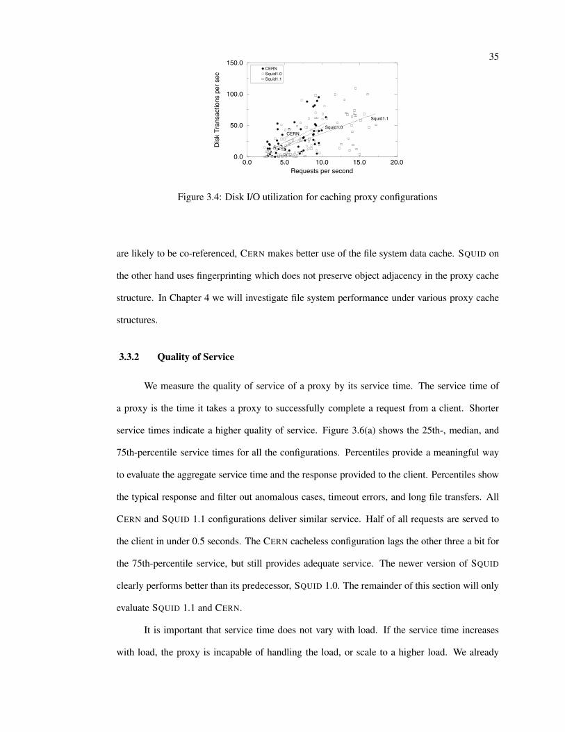
35
0.0 5.0 10.0 15.0 20.0Requests per second
0.0
50.0
100.0
150.0
Disk
Tra
nsac
tions
per
sec
CERNSquid1.0Squid1.1
Squid1.1
Squid1.0CERN
Figure 3.4: Disk I/O utilization for caching proxy configurations
are likely to be co-referenced, CERN makes better use of the file system data cache. SQUID on
the other hand uses fingerprinting which does not preserve object adjacency in the proxy cache
structure. In Chapter 4 we will investigate file system performance under various proxy cache
structures.
3.3.2 Quality of Service
We measure the quality of service of a proxy by its service time. The service time of
a proxy is the time it takes a proxy to successfully complete a request from a client. Shorter
service times indicate a higher quality of service. Figure 3.6(a) shows the 25th-, median, and
75th-percentile service times for all the configurations. Percentiles provide a meaningful way
to evaluate the aggregate service time and the response provided to the client. Percentiles show
the typical response and filter out anomalous cases, timeout errors, and long file transfers. All
CERN and SQUID 1.1 configurations deliver similar service. Half of all requests are served to
the client in under 0.5 seconds. The CERN cacheless configuration lags the other three a bit for
the 75th-percentile service, but still provides adequate service. The newer version of SQUID
clearly performs better than its predecessor, SQUID 1.0. The remainder of this section will only
evaluate SQUID 1.1 and CERN.
It is important that service time does not vary with load. If the service time increases
with load, the proxy is incapable of handling the load, or scale to a higher load. We already
36
saw that there are adequate system resources for an increased load. Figure 3.6(b) shows the
75th-percentile service time correlates with the requests/second load. There is no degradation
in serve time as the load increases. This is true for all percentile measures.
For a caching proxy configuration, the service times include both hits and misses. The
variance for hit service times is considerably lower than the variance of the miss service times.
To evaluate the impact of of hit rate on service, we plotted the hit rate with the requests/second
load. The hit rate is constant across load. The CERN cache hit rate is 35% SQUID 1.0 is 24%,
and the SQUID 1.1 hit rate is 28%. By comparing the service time distributions of caching and
cacheless configurations we can quantify the contribution of caching to the quality of service.
In a cacheless proxy configuration, service times consist only of miss times.
Figure 3.5 shows that in almost 90% of all cases the service time difference between a
caching and a cacheless configuration is less than a second. Thus, service times are not much
improved by caching. This is especially true for SQUID 1.1. CERN’s service time is more
sensitive to caching than other proxies. We conclude from this that caching is not as important
to service times as other aspects of proxy architectures. Figure 3.6 illustrates this more clearly:
the various percentile service times for CERN and SQUID 1.1 in a cacheless configuration do not
differ significantly from the corresponding caching configurations. However, across different
architectures, the service times are in some cases very different.
3.4 Discussion
In the light of SQUID’s sophisticated architecture we found the above results surprising.
SQUID and its predecessor, the Harvest Object Cache are perceived as at least an order of mag-
nitude faster than CERN [24, 125]. We found that the service times of CERN and SQUID are
about the same. The load used in the performance analysis of the Harvest Object Cache [24]
is very small compared to our load. The Harvest Object Cache’s architecture addresses perfor-
mance issues that are visible at low load, such as the elimination of context switches and the
introduction of the DNS cache. These features should also significantly improve performance
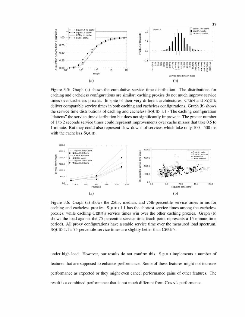
37
101 102 103 104 105
msec
0.00
0.25
0.50
0.75
1.00
cum
ulat
ive s
ervic
e tim
e di
strib
utio
n Squid 1.1 no cacheSquid 1.1 cacheCERN no cacheCERN cache
bin
= [0
,1)
[1,2
)[2
,4)
[4,8
)[8
,16)
[16,
32)
[32,
64)
[64,
128)
[128
,256
)[2
56.5
12)
[512
,1K)
[1K,
2K)
[2K,
4K)
[4K,
8K)
[8K,
16K)
[16K
,32K
)[3
2K,6
4K)
[64K
,128
K)[1
28K,
256K
)[2
56K,
512K
)[5
12K,
1M)−0.1
0.0
0.1
0.2
Frac
tion
of R
eque
sts
Squid 1.1 no cacheSquid 1.1 cachecache − no cache
Squid1.1
Service time bins in msec
(a) (b)
Figure 3.5: Graph (a) shows the cumulative service time distribution. The distributions forcaching and cacheless configurations are similar: caching proxies do not much improve servicetimes over cacheless proxies. In spite of their very different architectures, CERN and SQUIDdeliver comparable service times in both caching and cacheless configurations. Graph (b) showsthe service time distributions of caching and cacheless SQUID 1.1 - The caching configuration“flattens” the service time distribution but does not significantly improve it. The greater numberof 1 to 2 seconds service times could represent improvements over cache misses that take 0.5 to1 minute. But they could also represent slow-downs of services which take only 100 - 500 mswith the cacheless SQUID.
20.0 30.0 40.0 50.0 60.0 70.0 80.0Percentile
0.0
500.0
1000.0
1500.0
2000.0
2500.0
3000.0
Serv
ice T
ime
(mse
c)
Squid 1.1 No CacheSquid 1.1 CacheCERN no cacheCERN cacheSquid 1.0 No CacheSquid 1.0 Cache
0.0 5.0 10.0 15.0 20.0Requests per second
0.0
1000.0
2000.0
3000.0
4000.0
75−p
erce
ntile
ser
vice
time
[mse
c] Squid 1.1 cacheSquid 1.1 no cacheCERN cacheCERN no cache
(a) (b)
Figure 3.6: Graph (a) shows the 25th-, median, and 75th-percentile service times in ms forcaching and cacheless proxies. SQUID 1.1 has the shortest service times among the cachelessproxies, while caching CERN’s service times win over the other caching proxies. Graph (b)shows the load against the 75-percentile service time (each point represents a 15 minute timeperiod). All proxy configurations have a stable service time over the measured load spectrum.SQUID 1.1’s 75-percentile service times are slightly better than CERN’s.
under high load. However, our results do not confirm this. SQUID implements a number of
features that are supposed to enhance performance. Some of these features might not increase
performance as expected or they might even cancel performance gains of other features. The
result is a combined performance that is not much different from CERN’s performance.

38
With heavy real workload external network factors such as network latency become more
important. It is therefore important to isolate a proxy from the network as much as possible.
SQUID’s DNS caching is a good start: on a day with good DNS performance, SQUID’s DNS
caching saves on average 250 ms per request service time. However, our primary DNS server
occasionally has severe performance failures if its translation table exceeds the physical memory
size. In this case, a DNS lookup might take several seconds. SQUID’s DNS cache has a high hit
rate and therefore significantly reduces the impact of these DNS service malfunction on overall
proxy server performance.
Although hit rate is typically seen as an important factor for network latency and band-
width savings our results show it has a much more profound effect on reducing resource utiliza-
tion.
The following anecdote during our measurements also illustrates the importance of real
workload as opposed to artificial loads which do not account for wide-area network latencies:
as we mentioned earlier we observed an extreme two hour peak of 30K requests per 15 minutes
during a day at which we happened to monitor SQUID. During these two hours the average
service time and the average time spent on request errors dropped considerably and SQUID
used less resources than we expected. After studying the logs we found that the load had been
generated by a local web robot repeatedly accessing a local web server through the proxy. All
of these connections were fast and therefore did not consume many resources. This short period
made SQUID 1.0 appear as though it could easily scale up to 30K per 15 minutes, whereas our
results indicate that this is not the case. A benchmark such as the SPECweb96 [113] would test
a proxy under conditions that are similar to this incident.
3.5 Conclusions
Implementation is at least as an important factor in performance as architecture. SQUID’s
sophisticated architecture should significantly improve performance under high load. However,
our results do not confirm this and some of SQUID’s features are often costly to implement. For
39
instance, SQUID uses the CPU cycles it saved by not forking processes to implement memory
management and non-blocking network communication. CERN’s architecture is inherently in-
efficient, but manages to efficiently use underlying operating systems constructs. As a result
CERN has comparable performance.
With cache hit rates of around 30% we were unable to see a significant difference in the
service time profiles between caching and cacheless proxy configurations. Caching might have a
larger impact on service times at sites with less available bandwidth than our test site, Although
hit rate is typically seen as an important factor for network latency and bandwidth savings our
results show it has a much more profound effect on reducing the resource utilization.
CERN uses memory for process state such that its memory utilization grows linearly with
the number of processes that are required to support a given request load. SQUID keeps global
cache and process state in main memory. This state is largely independent of load. CERN and
SQUID use the same amount of memory at around 20 to 25 requests per second. CERN requires
less memory than SQUID at a load below 20 requests per second while SQUID is likely to require
less memory than CERN at a load above 25 requests per second. Poor network connectivity is
likely to lower the indifference point.
Although SQUID has many features designed to reduce disk traffic, our measurements did
not show any discernable difference between the two architectures. As we will see in Chapter 4
the CERN access patterns maps very well to the file system caching strategy, and the operating
system effectively eliminates many of the potential CERN disk accesses.
Another important aspect of this study is the large, diurnal variation of workload. Other
studies such as [107] and [55] confirm that this workload variation is characteristic for enterprise-
level web proxy servers. To our knowledge, no web proxy server is able to take advantage of
unused resources during off-peak periods in order to reduce resource utilization during peak
periods. In Chapter 5 and Chapter 6 we will introduce techniques that will take advantage of
extra resources availabe during off-peak time.
Chapter 4
Reducing the Disk I/O of Web Proxy Server Caches
4.1 Introduction
With the availability of faster processors and cheaper main memory, the common bottle-
neck of today’s large Web proxy servers is disk I/O [4, 107, 124]. One could store the entire
cache in main memory. However, web caching frequently requires large cache sizes in the order
of 10G Bytes (see Chapter 2). Maintaining a cache of this size in primary memory is often still
infeasible.
Until main memory becomes cheap enough, Web caches will use disks, so there is a
strong interest in reducing the overhead of disk I/O. Some commercial Web proxy servers come
with hardware and a special operating system that is optimized for disk I/O. However, these
solutions are expensive and in many cases not affordable. There is a wide interest in portable,
low-cost solutions which require not more than standard off-the-shelf hardware and software.
In this paper we are interested in exploring ways to reduce disk I/O by changing the way a Web
proxy server application utilizes a general-purpose Unix file system using standard Unix system
calls.
In this Chapter we compare the file system interactions of two existing Web proxy
servers, CERN [76] and SQUID [123]. We show how adjustments to the current SQUID cache
architecture can dramatically reduce disk I/O.
Our findings suggest that two strategies can significantly reduce disk I/O: (1) preserve
locality of the HTTP reference stream while translating these references into cache references,
41
and (2) use virtual memory instead of the file system for objects smaller than the system page
size. We support our claims using measurements from actual file systems exercised by a trace
driven workload collected from proxy server log data at a major corporate Internet gateway.
4.2 Cache Architectures of Web Proxy Servers
We define the cache architecture of a Web proxy server as the way a proxy server
interacts with a file system. A cache architecture names, stores, and retrieves objects from a file
system, and maintains application-level meta-data about cached objects.
To better understand the impact of cache architectures on file systems we first review
the basic design goals of file systems and then describe the Unix Fast File System (FFS), the
standard file system available on most variants of the UNIX operating system.
4.2.1 The Unix Fast File System
Since the speed of disks lags far behind the speed of main memory the most important
factor in I/O performance is whether disk I/O occurs at all ([60], page 542). File systems use
memory caches to reduce disk I/O. The file system provides a buffer cache and a name cache.
The buffer cache serves as a place to transfer and cache data to and from the disk. The name
cache stores file and directory name resolutions which associate file and directory names with
file system data structures that otherwise reside on disk.
The Fast File System (FFS) [81] divides disk space into blocks of uniform size (either
four or eight kilobytes). These are the basic units of disk space allocation. These blocks may
be sub-divided into fragments of 1 kilobytes for small files or files that require a non-integral
number of blocks.
Blocks are grouped into cylinder groups which are sets of typically sixteen adjacent
cylinders. These cylinder groups are used to map file reference locality to physically adjacent
disk space. FFS tries to store each directory and its content within one cylinder group and each
file into a set of adjacent blocks. The FFS does not guarantee such file layout but uses a simple
42
set of heuristics to achieve it. As the file system fills up, the FFS will increasingly often fail
to maintain such a layout and the file system gets increasingly fragmented. A fragmented file
system stores a large part of its files in non-adjacent blocks. Reading and writing data from and
to non-adjacent blocks causes longer seek times and can severely reduce file system throughput.
Each file is described by meta-data in the form of inodes. An inode is a fixed length
structure that contains information about the size and location of the file as well as up to fifteen
pointers to the blocks which store the data of the file. The first 12 pointers are direct pointers
while the last three pointers refer to indirect blocks, which contain pointers to additional file
blocks or to additional indirect blocks. The vast majority of files are shorter than 96 kilobytes,
so in most cases an inode can directly point to all blocks of a file, and storing them within the
same cylinder group further exploits this reference locality.
The design of the FFS reflects assumption about file system workloads. These assump-
tions are based on studies of workloads generated by workstations [93, 103]. These workstation
workloads and Web cache request workloads share many, but not all of the same characteristics.
Because most of their behavior is similar, the file system works reasonably well for caching
Web pages. However there are differences; and tweaks to to the way cache objects map onto
the file system produce significant performance improvements.
We will show in the following sections that some file system aspects of the workload
characteristics generated by certain cache architectures can differ from usual workstation work-
loads. These different workload characteristics lead to poor file system performance. We will
also show that adjustments to cache architectures can dramatically improve file system perfor-
mance.
4.2.2 File System Aspects of Web Proxy Server Cache Workloads
The basic function of a Web proxy server is to receive a request from a client, check
whether the request is authorized, and serve the requested object either from a local disk or
from the Internet. Generally, objects served from the Internet are also stored on a local disk so
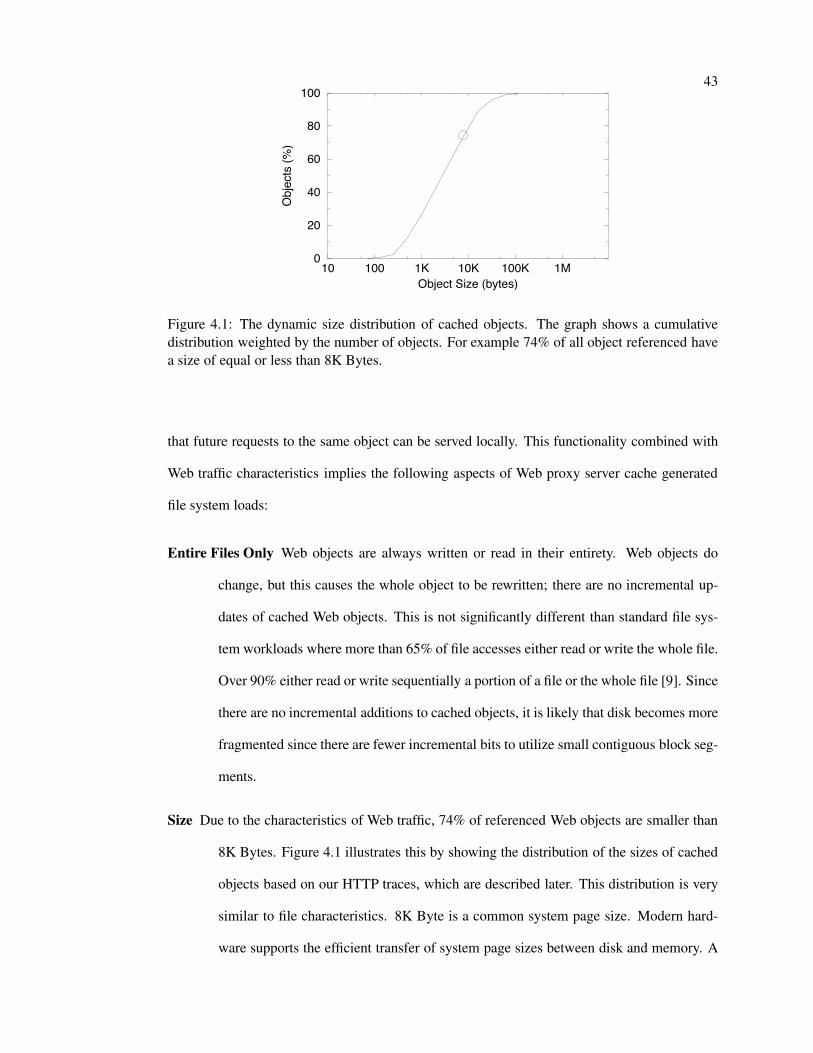
43
10 100 1K 10K 100K 1MObject Size (bytes)
0
20
40
60
80
100
Obj
ects
(%)
Figure 4.1: The dynamic size distribution of cached objects. The graph shows a cumulativedistribution weighted by the number of objects. For example 74% of all object referenced havea size of equal or less than 8K Bytes.
that future requests to the same object can be served locally. This functionality combined with
Web traffic characteristics implies the following aspects of Web proxy server cache generated
file system loads:
Entire Files Only Web objects are always written or read in their entirety. Web objects do
change, but this causes the whole object to be rewritten; there are no incremental up-
dates of cached Web objects. This is not significantly different than standard file sys-
tem workloads where more than 65% of file accesses either read or write the whole file.
Over 90% either read or write sequentially a portion of a file or the whole file [9]. Since
there are no incremental additions to cached objects, it is likely that disk becomes more
fragmented since there are fewer incremental bits to utilize small contiguous block seg-
ments.
Size Due to the characteristics of Web traffic, 74% of referenced Web objects are smaller than
8K Bytes. Figure 4.1 illustrates this by showing the distribution of the sizes of cached
objects based on our HTTP traces, which are described later. This distribution is very
similar to file characteristics. 8K Byte is a common system page size. Modern hard-
ware supports the efficient transfer of system page sizes between disk and memory. A

44
number of Unix File Systems use a file system block size of 8K and a fragment size
of 1K. Typically the performance of the file system’s fragment allocation mechanism
has a greater impact on overall performance than the block allocation mechanism. In
addition, fragment allocation is often more expensive than block allocation because
fragment allocation usually involves a best-fit search.
Popularity The popularity of Web objects follows a Zipf-like distribution [53, 19]. The rel-
ative popularity of objects changes slowly (on the order of days and weeks). This
implies that for any given trace of Web traffic, the first references to popular objects
within a trace tend to occur early in the trace. The slow migration to new popular items
allows for relatively static working set capture algorithms (see for example [110]). It
also means that there is little or no working set behavior attributable to the majority
of the referenced objects. File system references exhibit much more temporal locality;
allocation and replacement policies need to react rapidly to working set changes.
Data Locality A large number of Web objects include links to embedded objects that are ref-
erenced in short succession. These references commonly refer to the same server and
tend to even have the same URL prefix. This is similar to the locality observed in
workstation workloads which show that files accessed in short succession tend to be in
the same file directory.
Meta-data Locality The fact that objects with similar names tend to be accessed in short suc-
cession means that information about those objects will also be referenced in short
succession. If the information required to validate and access files is combined in the
same manner as the file accesses it will exhibit temporal locality (many re-references
within a short time period). The hierarchal directory structure of files systems tends to
group related files together. The meta-data about those files and their access methods
are stored in directory and inodes which end up being highly reused when accessing a
group of files. Care is required to properly map Web objects to preserve the locality of
45
meta-data.
Read/Write Ratio The hit rate of Web caches is low (30%-50%, see Chapter 2). Every cache
hit involves a read of the cache meta-data and a read of the cached data. Every miss
involves a read of the cache meta-data, a write of meta-data, and a write of the Web
object. Since there are typically more misses than hits, the majority of disk accesses are
writes. File systems typically have many more reads than writes [93]; writes require
additional work because the file system data must be properly flushed from memory
to disk. The high fraction of writes also causes the disk to quickly fragment. Data is
written, removed and rewritten quickly; this makes it difficult to keep contiguous disk
blocks available for fast or large data writes.
Redundancy Cached Web objects are (and should be) redundant; individual data items are not
critical for the operation of Web proxy caches. If the cached data is lost, it can always
be served from the Internet. This is not the case with file system data. Data lost before
it is securely written to disk is irrecoverable. With highly reliable Web proxy servers
(both software and hardware) it is acceptable to never actually store Web objects to
disk, or to periodically store all Web objects to disk in the event of a server crash. This
can significantly reduce the memory system page replacement cost for Web objects. A
different assessment has to be made for the meta data which some web proxy server
use for cache management. In the event of meta data loss, either the entire content
of the cache is lost or has to be somehow rebuilt based on data saved on disk. High
accessibility requirements might neither allow the loss of the entire cache nor time
consuming cache rebuilds. In that case meta data has to be handled similarly to file
system data. The volume of meta data is however much smaller than the volume of
cached data.
46
4.2.3 Cache Architectures of Existing Web Proxy Servers
We use CERN and SQUID as baseline architectures for our investigations. The general
differences between these architectures are explained in Chapter 2. The following reviews archi-
tecture details that are relevant for this Chapter. We then describe how the SQUID architecture
could be changed to improve performance. All architectures assume infinite cache sizes. We
discuss the management of finite caches in Chapter 5.
4.2.3.1 CERN
The forked processes of CERN use the file system not only to store cached copies of
Web objects but also to share meta-information about the content of the cache and to coordinate
access to the cache. To find out whether a request can be served from the cache, CERN first
translates the URL of the request into a URL directory (as described in Chapter 2) and checks
whether a lock file for the requested URL exists. This checks requires the translation of each
path component of the URL directory into an inode. Each translation can cause a miss in the
file system’s name cache in which case the translation requires information from the disk.
The existence of a lock file indicates that another CERN process is currently inserting the
requested object into the cache. Locked objects are not served from the cache but fetched from
the Internet without updating the cache. If no lock file exists, CERN tries to open the meta-
data file in the URL directory. A failure to do so indicates a cache miss in which case CERN
fetches the object from the Internet and inserts it into the cache thereby creating the necessary
directories, temporary lock files, and meta-data files. All these operations require additional
disk I/O in the case of misses in the file system’s name and buffer cache. If the meta-data file
exists and it lists the object file name as not expired, CERN serves the request from the cache.
4.2.3.2 SQUID
SQUID keeps meta-data about the cache contents in main memory. Each entry of the
47
the meta-data maps a URL to a unique file number and contains data about the “freshness”
of the cached object. If the meta-data does not contain an entry for the requested URL or the
entry indicates that the cached copy is stale, the object is fetched from the Internet and inserted
into the cache. Thus, with in-memory meta-data the disk is never touched to find out whether a
request is a Web cache miss or a Web cache hit.
A unique file number n maps to a two-level file path that contains the cached object. The
file path follows from the unique file number using the formula
(x, y, z) = (n mod l1, n/l1 mod l2, n)
where (x, y, z) maps to the file path “x/y/z”, and l1 and l2 are the numbers of first and second
level directories. Unique file numbers for new objects are generated by either incrementing
a global variable or reusing numbers from expired objects. This naming scheme ensures that
the resulting directory tree is balanced. The number of first and second level directories are
configurable to ensure that directories do not become too large. If directory objects exceed the
size of a file block, directory look-up times increase.
4.2.4 Variations on the SQUID Cache Architecture
The main difference between CERN and SQUID is that CERN stores all state on disk
while SQUID keeps a representation of the content of its cache (the metadata) in main memory.
It would seem straightforward to assume that CERN’s architecture causes more disk I/O than
SQUID’s architecture. However, as we showed in Chapter 3 (and [77]), CERN’s and SQUID’s
disk I/O are surprisingly similar for the same workload.
Our conjecture was that this is due to the fact that CERN’s cache architecture preserves
some of the locality of the HTTP reference stream, while SQUID’s unique numbering scheme
destroys locality. Although the CERN cache has a high file system overhead, the preservation
of the spatial locality seen in the HTTP reference stream leads to a disk I/O performance com-
parable to the SQUID cache.
48
We have designed two alternative cache architectures for the SQUID cache that improve
reference locality. We also investigated the benefits of circumventing the common file sys-
tem abstractions for storing and retrieving objects by implementing memory-mapped caches.
Memory mapped caches can reduce the number of file-system system calls and effectively use
large primary memories. However, memory-mapped caches also introduce more complexity
for placement and replacement policies. We will examine several such allocation policies.
4.2.4.1 SQUIDL
We designed a modified SQUID cache architecture, SQUIDL, to determine whether a
locality-preserving translation of an HTTP reference stream into a file system access stream
reduces disk I/O. The only difference between SQUID and SQUIDL is that SQUIDL derives the
URL directory name from the URL’s host name instead of calculating a unique number. The
modified formula for the file path of a cached object is now
(x, y, z) = (h(s) ∧ml1 , h(s) ∧ml2 , n)
where s is the host name of the requested URL, h is a hash function, ∧ is the bitwise conjunction,
ml1 a bit mask for the first level directories, and ml2 for the second level directories.
The rationale of this design is based on observation of the data shown in figure 4.2 (based
on our HTTP traces, see below): the temporal locality of server names in HTTP references is
high. One explanation for this is the fact that a large portion of HTTP requests are for objects
that are embedded in the rendition of a requested HTML object. HTTP clients request these
“inlined” objects immediately after they parsed the HTML object. In most HTML objects all
inlined objects are from the same server. Since SQUIDL stores cached objects of the same
server in the same directory, cache references to linked objects will tend to access the same
directory. This leads to a burst of requests to the same directory and therefore increases the
temporal locality of file system requests.
One drawback of SQUIDL is that a single directory may store many objects from a pop-
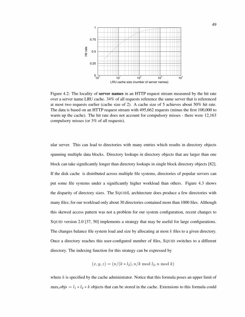
49
100 101 102 103 104
LRU cache size (number of server names)
0
0.25
0.5
0.75
1
Hit r
ate
Figure 4.2: The locality of server names in an HTTP request stream measured by the hit rateover a server name LRU cache. 34% of all requests reference the same server that is referencedat most two requests earlier (cache size of 2). A cache size of 5 achieves about 50% hit rate.The data is based on an HTTP request stream with 495,662 requests (minus the first 100,000 towarm up the cache). The hit rate does not account for compulsory misses - there were 12,163compulsory misses (or 3% of all requests).
ular server. This can lead to directories with many entries which results in directory objects
spanning multiple data blocks. Directory lookups in directory objects that are larger than one
block can take significantly longer than directory lookups in single block directory objects [82].
If the disk cache is distributed across multiple file systems, directories of popular servers can
put some file systems under a significantly higher workload than others. Figure 4.3 shows
the disparity of directory sizes. The SQUIDL architecture does produce a few directories with
many files; for our workload only about 30 directories contained more than 1000 files. Although
this skewed access pattern was not a problem for our system configuration, recent changes to
SQUID version 2.0 [37, 50] implements a strategy that may be useful for large configurations.
The changes balance file system load and size by allocating at most k files to a given directory.
Once a directory reaches this user-configured number of files, SQUID switches to a different
directory. The indexing function for this strategy can be expressed by
(x, y, z) = (n/(k ∗ l2), n/k mod l2, n mod k)
where k is specified by the cache administrator. Notice that this formula poses an upper limit of
max objs = l1 ∗ l2 ∗ k objects that can be stored in the cache. Extensions to this formula could
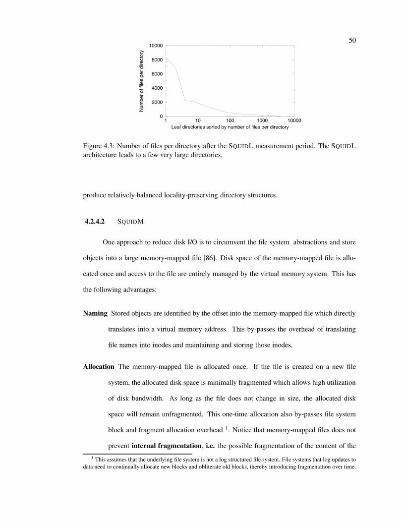
50
1 10 100 1000 10000Leaf directories sorted by number of files per directory
0
2000
4000
6000
8000
10000
Num
ber o
f file
s pe
r dire
ctor
yFigure 4.3: Number of files per directory after the SQUIDL measurement period. The SQUIDLarchitecture leads to a few very large directories.
produce relatively balanced locality-preserving directory structures.
4.2.4.2 SQUIDM
One approach to reduce disk I/O is to circumvent the file system abstractions and store
objects into a large memory-mapped file [86]. Disk space of the memory-mapped file is allo-
cated once and access to the file are entirely managed by the virtual memory system. This has
the following advantages:
Naming Stored objects are identified by the offset into the memory-mapped file which directly
translates into a virtual memory address. This by-passes the overhead of translating
file names into inodes and maintaining and storing those inodes.
Allocation The memory-mapped file is allocated once. If the file is created on a new file
system, the allocated disk space is minimally fragmented which allows high utilization
of disk bandwidth. As long as the file does not change in size, the allocated disk
space will remain unfragmented. This one-time allocation also by-passes file system
block and fragment allocation overhead 1. Notice that memory-mapped files does not
prevent internal fragmentation, i.e. the possible fragmentation of the content of the1 This assumes that the underlying file system is not a log structured file system. File systems that log updates to
data need to continually allocate new blocks and obliterate old blocks, thereby introducing fragmentation over time.
51
memory-mapped file due to application-level data management of the data stored in
memory-mapped files. Since we assume infinite caches, internal fragmentation is not
an issue here. See Chapter 5 for the management of finite memory-mapped caches.
Paging Disk I/O is managed by virtual memory which takes advantage of hardware optimized
for paging. The smallest unit of disk I/O is a system page instead of the size of the
smallest stored object.
Thus, we expect that memory-mapping will benefit us primarily in the access of small
objects by eliminating the opening and closing of small files. Most operating systems have
limits on the size of memory-mapped files, and care must be taken to appropriately choose the
objects to store in the limited space available. In the cache architecture SQUIDM we therefore
chose the system page size (8K Byte) as upper limit. Over over 70% of all object references are
less or equal than 8K bytes (see figure 4.1 which is based on our HTTP traces). Objects larger
than 8Kbytes are cached the same way as in SQUID.
To retrieve an object from a memory-mapped file we need to have its offset into the
memory-mapped file and its size. In SQUIDM offset and size of each object are stored in in-
memory meta-data. Instead of keeping track of the actual size of an object we defined five
segment sizes (512, 1024, 2048, 4,096, or 8,192 Bytes). This reduces the size information from
thirteen bits down to three bits. Each object is padded to the smallest segment size. In Chapter 5
we will show more advantages of managing segments instead of object sizes.
These padded objects are contiguously written into the mapped virtual memory area in
the order in which they are first referenced (and thus missed). Our conjecture was that this
strategy would translate the temporal locality of the HTTP reference stream into spatial locality
of virtual memory references.
We will show that this strategy also tends to concentrate very popular objects in the
first few pages of the memory-mapped file; truly popular objects will be referenced frequently
enough to be at the beginning of any reference stream. Clustering popular objects significantly
52
reduces the number of page faults since those pages tend to stay in main memory. Over time, the
set of popular references may change, increasing the page fault rate. In Chapter 5 we explore
compaction methods to improve reference locality.
4.2.4.3 SQUIDML
The SQUIDML architecture uses a combination of SQUIDM for objects smaller than 8K
Byte and SQUIDL for all other objects.
4.2.4.4 SQUIDMLA
The SQUIDMLA architecture combines the SQUIDML architecture with an algorithm
to align objects in the memory mapped file such that no object crosses a page boundary. An
important requirement of such an algorithm is that it preserves reference locality. We use a
packing algorithm, shown in Algorithm 1 that for the given traces only slightly modifies the
order in which objects are stored in the memory-mapped file. The algorithm insures that no
object crosses page boundaries.
Given a list of object sizes of which none is greater than 8K Bytes, the algorithm gen-
erates a corresponding list of offsets which are aligned to 1K, 2K, 4K, and 8K Bytes blocks.
The algorithm maintains five offset pointers which point to the lowest available offset for each
of the five segment sizes. Zero values of the first four pointers indicate that no segment of the
corresponding size is available and that a segment of the next available larger size needs to be
broken up. For example, if the first four values are zero and the segment size of the current
object is 512 Bytes, the offset returned for the object is the value of the fifth pointer. The fifth
pointer is then incremented by 8K, the first pointer is set to offset + 512, the second pointer to
offset +1K, the third pointer to offset +2K, and the fourth pointer to offset +4K. If the next
object is of segment size 1K Bytes, the value of the second pointer is returned as offset and the
pointer is set to zero. If then the next object is another 1K object, the value of the third pointer
is returned as offset, the third pointer is set to zero, and the second pointer is set to the returned
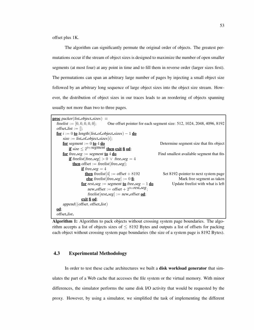
53
offset plus 1K.
The algorithm can significantly permute the original order of objects. The greatest per-
mutations occur if the stream of object sizes is designed to maximize the number of open smaller
segments (at most four) at any point in time and to fill them in reverse order (larger sizes first).
The permutations can span an arbitrary large number of pages by injecting a small object size
followed by an arbitrary long sequence of large object sizes into the object size stream. How-
ever, the distribution of object sizes in our traces leads to an reordering of objects spanning
usually not more than two to three pages.
proc packer(list object sizes) ≡freelist := [0, 0, 0, 0, 0]; One offset pointer for each segment size: 512, 1024, 2048, 4096, 8192offset list := [];for i := 0 to length(list of object sizes)− 1 do
size := list of object sizes[i];for segment := 0 to 4 do Determine segment size that fits object
if size ≤ 29+segment then exit fi od;for free seg := segment to 4 do Find smallest available segment that fits
if freelist [free seg] > 0 ∨ free seg = 4then offset := freelist [free seg];
if free seg = 4then freelist [4] := offset + 8192 Set 8192-pointer to next system pageelse freelist [free seg] := 0 fi; Mark free segment as taken
for rest seg := segment to free seg − 1 do Update freelist with what is leftnew offset := offset + 29+rest seg ;freelist [rest seg] := new offset od;
exit fi od;append((offset , offset list)
od;offset list .
Algorithm 1: Algorithm to pack objects without crossing system page boundaries. The algo-rithm accepts a list of objects sizes of ≤ 8192 Bytes and outputs a list of offsets for packingeach object without crossing system page boundaries (the size of a system page is 8192 Bytes).
4.3 Experimental Methodology
In order to test these cache architectures we built a disk workload generator that sim-
ulates the part of a Web cache that accesses the file system or the virtual memory. With minor
differences, the simulator performs the same disk I/O activity that would be requested by the
proxy. However, by using a simulator, we simplified the task of implementing the different
54
allocation and replacement policies and greatly simplified our experiments. Using a simulator
rather than a proxy allows us to use traces of actual cache requests without having to mimic the
full Internet. Thus, we could run repeatable measurements on the cache component we were
studying – the disk I/O system.
The workload generators are driven by actual HTTP Web proxy server traces. Each trace
entry consists of a URL and the size of the referenced object. During an experiment a workload
generator sequentially processes each trace entry – the generator first determines whether a
cached object exists and then either “misses” the object into the cache by writing data of the
specified size to the appropriate location or “hits” the object by reading the corresponding data.
Our workload generators process requests sequentially and thus our experiments do not account
for the fact that the CERN and SQUID architecture allow multiple files to be open at the same
time and that access to files can be interleaved. Unfortunately this hides possible file system
locking issues.
We ran all experiments on a dedicated Digital Alpha Station 250 4/266 with 512M Byte
main memory. We used two 4G Byte disks and one 2G Byte disk to store cached objects. We
used the UFS file system that comes with Digital Unix 4.0 for all experiments except those that
calibrate the experiments in this paper to those in earlier work. The UFS file system uses a
block size of 8192 Bytes and a fragment size of 1024 Bytes. For the comparison of SQUID and
CERN we used Digital’s Advanced File System (AdvFS) to validate our experiments with the
results presented in Chapter 3.
UFS cannot span multiple disks so we needed a separate file system for each disk. All
UFS experiments measured SQUID derived architectures with 16 first-level directories and 256
second-level directories. These 4096 directories were distributed over the three file systems,
820 directories on the 2G Byte disk and 1638 directories on each of the 4G Byte disks. When
using memory-mapped caches, we placed 2048 directories on each 4G Byte disk and used
the 2G Byte disk exclusively for the memory-mapped file. This also allowed us to measure
memory-mapped-based caching separately from file-system-based caching.
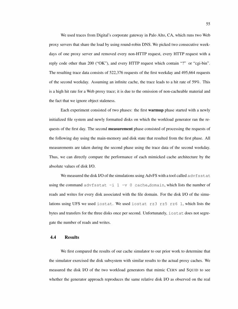
55
We used traces from Digital’s corporate gateway in Palo Alto, CA, which runs two Web
proxy servers that share the load by using round-robin DNS. We picked two consecutive week-
days of one proxy server and removed every non-HTTP request, every HTTP request with a
reply code other than 200 (“OK”), and every HTTP request which contain “?” or “cgi-bin”.
The resulting trace data consists of 522,376 requests of the first weekday and 495,664 requests
of the second weekday. Assuming an infinite cache, the trace leads to a hit rate of 59%. This
is a high hit rate for a Web proxy trace; it is due to the omission of non-cacheable material and
the fact that we ignore object staleness.
Each experiment consisted of two phases: the first warmup phase started with a newly
initialized file system and newly formatted disks on which the workload generator ran the re-
quests of the first day. The second measurement phase consisted of processing the requests of
the following day using the main-memory and disk state that resulted from the first phase. All
measurements are taken during the second phase using the trace data of the second weekday.
Thus, we can directly compare the performance of each mimicked cache architecture by the
absolute values of disk I/O.
We measured the disk I/O of the simulations using AdvFS with a tool called advfsstat
using the command advfsstat -i 1 -v 0 cache domain, which lists the number of
reads and writes for every disk associated with the file domain. For the disk I/O of the simu-
lations using UFS we used iostat. We used iostat rz3 rz5 rz6 1, which lists the
bytes and transfers for the three disks once per second. Unfortunately, iostat does not segre-
gate the number of reads and writes.
4.4 Results
We first compared the results of our cache simulator to our prior work to determine that
the simulator exercised the disk subsystem with similar results to the actual proxy caches. We
measured the disk I/O of the two workload generators that mimic CERN and SQUID to see
whether the generator approach reproduces the same relative disk I/O as observed on the real
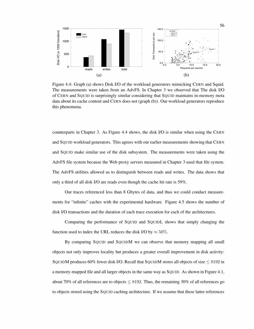
56
reads writes total0
500
1000
1500
Disk
I/O
(x 1
000
trans
fers
)
CernSquid
0.0 5.0 10.0 15.0 20.0Requests per second
0.0
50.0
100.0
150.0
Disk
Tra
nsac
tions
per
sec
CERNSquid1.0Squid1.1
Squid1.1
Squid1.0CERN
(a) (b)
Figure 4.4: Graph (a) shows Disk I/O of the workload generators mimicking CERN and Squid.The measurements were taken from an AdvFS. In Chapter 3 we observed that The disk I/Oof CERN and SQUID is surprisingly similar considering that SQUID maintains in-memory metadata about its cache content and CERN does not (graph (b)). Our workload generators reproducethis phenomena.
counterparts in Chapter 3. As Figure 4.4 shows, the disk I/O is similar when using the CERN
and SQUID workload generators. This agrees with our earlier measurements showing that CERN
and SQUID make similar use of the disk subsystem. The measurements were taken using the
AdvFS file system because the Web proxy servers measured in Chapter 3 used that file system.
The AdvFS utilities allowed us to distinguish between reads and writes. The data shows that
only a third of all disk I/O are reads even though the cache hit rate is 59%.
Our traces referenced less than 8 Gbytes of data, and thus we could conduct measure-
ments for “infinite” caches with the experimental hardware. Figure 4.5 shows the number of
disk I/O transactions and the duration of each trace execution for each of the architectures.
Comparing the performance of SQUID and SQUIDL shows that simply changing the
function used to index the URL reduces the disk I/O by ≈ 50%.
By comparing SQUID and SQUIDM we can observe that memory mapping all small
objects not only improves locality but produces a greater overall improvement in disk activity:
SQUIDM produces 60% fewer disk I/O. Recall that SQUIDM stores all objects of size ≤ 8192 in
a memory-mapped file and all larger objects in the same way as SQUID. As shown in Figure 4.1,
about 70% of all references are to objects ≤ 8192. Thus, the remaining 30% of all references go
to objects stored using the SQUID caching architecture. If we assume that these latter references
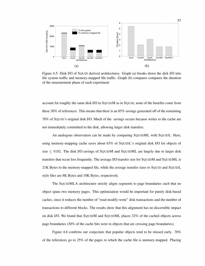
57
Squid SquidL SquidM SquidML SquidMLAArchitecture
0
1000
2000
3000
Disk
I/O
[100
0 tra
nsfe
rs] To file system
To memory−mapped file
Squid SquidM SquidL SquidML SquidMLAArchitecture
0
1
2
3
4
5
6
Dura
tion
[hou
r]
(a) (b)
Figure 4.5: Disk I/O of SQUID derived architectures. Graph (a) breaks down the disk I/O intofile system traffic and memory-mapped file traffic. Graph (b) compares compares the durationof the measurement phase of each experiment
account for roughly the same disk I/O in SQUIDM as in SQUID, none of the benefits come from
these 30% of references. This means that there is an 85% savings generated off of the remaining
70% of SQUID’s original disk I/O. Much of the savings occurs because writes to the cache are
not immediately committed to the disk, allowing larger disk transfers.
An analogous observation can be made by comparing SQUIDML with SQUIDL. Here,
using memory-mapping cache saves about 63% of SQUIDL’s original disk I/O for objects of
size ≤ 8192. The disk I/O savings of SQUIDM and SQUIDML are largely due to larger disk
transfers that occur less frequently. The average I/O transfer size for SQUIDM and SQUIDML is
21K Bytes to the memory-mapped file, while the average transfer sizes to SQUID and SQUIDL
style files are 8K Bytes and 10K Bytes, respectively.
The SQUIDMLA architecture strictly aligns segments to page boundaries such that no
object spans two memory pages. This optimization would be important for purely disk-based
caches, since it reduces the number of “read-modify-write” disk transactions and the number of
transactions to different blocks. The results show that this alignment has no discernible impact
on disk I/O. We found that SQUIDM and SQUIDML places 32% of the cached objects across
page boundaries (30% of the cache hits were to objects that are crossing page boundaries).
Figure 4.6 confirms our conjecture that popular objects tend to be missed early. 70%
of the references go to 25% of the pages to which the cache file is memory-mapped. Placing
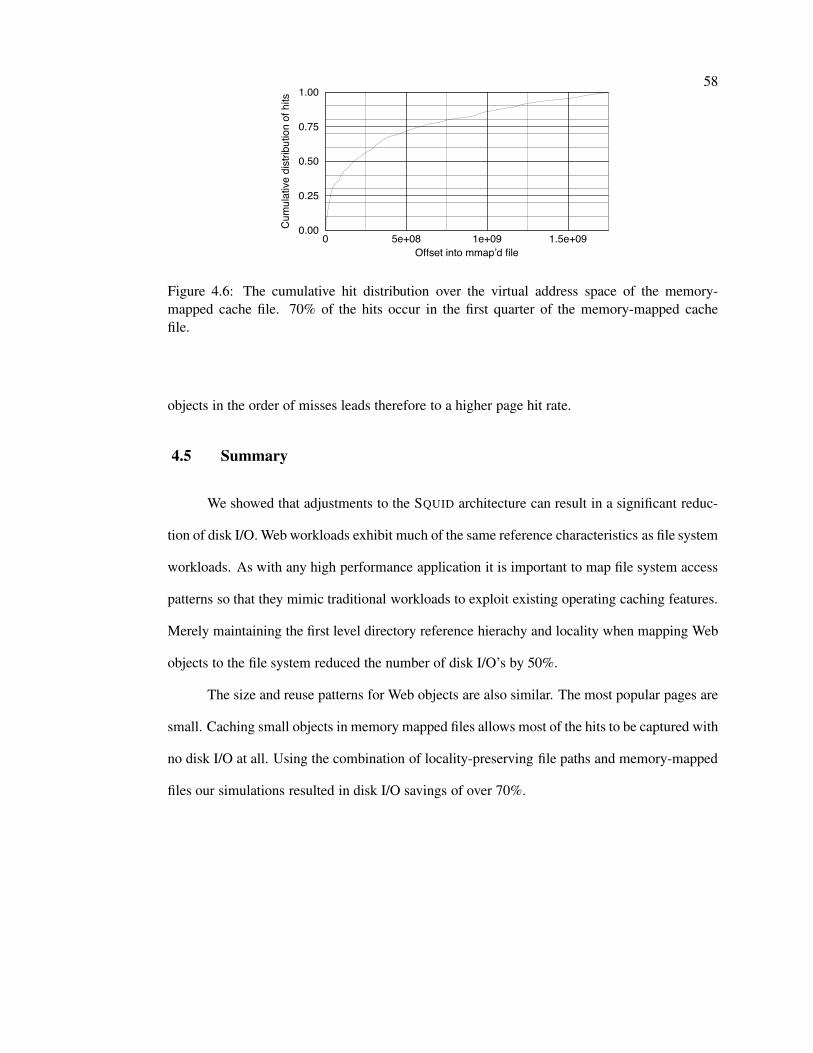
58
0 5e+08 1e+09 1.5e+09Offset into mmap’d file
0.00
0.25
0.50
0.75
1.00
Cum
ulat
ive d
istrib
utio
n of
hits
Figure 4.6: The cumulative hit distribution over the virtual address space of the memory-mapped cache file. 70% of the hits occur in the first quarter of the memory-mapped cachefile.
objects in the order of misses leads therefore to a higher page hit rate.
4.5 Summary
We showed that adjustments to the SQUID architecture can result in a significant reduc-
tion of disk I/O. Web workloads exhibit much of the same reference characteristics as file system
workloads. As with any high performance application it is important to map file system access
patterns so that they mimic traditional workloads to exploit existing operating caching features.
Merely maintaining the first level directory reference hierachy and locality when mapping Web
objects to the file system reduced the number of disk I/O’s by 50%.
The size and reuse patterns for Web objects are also similar. The most popular pages are
small. Caching small objects in memory mapped files allows most of the hits to be captured with
no disk I/O at all. Using the combination of locality-preserving file paths and memory-mapped
files our simulations resulted in disk I/O savings of over 70%.

Chapter 5
Management of Memory-mapped Web Caches
5.1 Introduction
In Chapter 4 we show that storing small objects in a memory-mapped file can signifi-
cantly reduce disk I/O. We assumed infinite cache size and therefore did not address replace-
ment strategies. In this Chapter we explore the effect of replacement strategies on disk I/O of
finite cache achitectures which use memory-mapped files.
Cache architectures which use the file system to cache objects to either individual files
or one memory-mapped file are really two-level cache architectures: the first-level cache is the
buffer cache in the primary memory and the second-level cache is the disk. However, standard
operating systems generally do not support sufficient user-level control on buffer cache man-
agement to control primary memory replacement. This leaves us with the problem of replacing
objects in secondary memory in such a way that disk I/O is minimized.
In the following sections we first review relevant aspects of system-level management
of memory-mapped files. We then introduce three replacement algorithms and evaluate their
performance.
5.2 Memory-mapped Files
A memory-mapped file is represented in the virtual memory system as a virtual memory
object associated with a pager. A pager is responsible for filling and cleaning pages from and
to a file. In older Unix systems the pager would operate on top of the file system. Because
60
the virtual memory system and the file system used to be two independent systems, this led to
the duplication of each page of a memory-mapped file. One copy would be stored in a buffer
managed by the buffer cache and another in a page frame managed by the virtual memory. This
duplication is not only wasteful but also leads to cache inconsistencies. Newer Unix imple-
mentations have a “unified buffer cache” where loaded virtual memory pages and buffer cache
buffers can refer to the same physical memory location.
If access to a virtual memory address causes a page fault, the page fault handler is se-
lecting a target page and passes control to the pager which is responsible for filling the page
with the appropriate data. A pager translates the virtual memory address which caused the page
fault into the memory-mapped file offset and retrieves the corresponding data from disk.
In the context of memory-mapped files, a page is dirty if it contains information that
differs from the corresponding part of the file stored on disk. A page is clean if its information
matches the information on the associated part of the file on disk. We call the process of writing
dirty pages to disk cleaning. If the target page of a page fault is dirty it needs to be cleaned
before it can be handed to the pager. Dirty pages are also cleaned periodically, typically every
30 seconds.
Except for very large files the latency of a disk transaction does not depend on the amount
of data transferred but on disk arm repositioning and rotational delays. The file system as well as
disk drivers and disk hardware are designed to minimize disk arm repositioning and rotational
delays for a given access stream by reordering access requests depending on the current position
of the disk arm and the current disk sector. However, reordering can only occur to a limited
extent. Disk arm repositioning and rotational delays are still mainly dependent on the access
pattern of the access stream and the disk layout.
Studies on file systems (e.g. [93]) have shown that the majority of file system access is a
sequential access of logically adjacent data blocks. File systems therefore establish disk layout
which is optimized for sequential access by placing logically adjacent blocks into physically
adjacent sectors of the same cylinder whenever possible [82]. Thus, a sequential access stream
61
minimizes disk arm repositioning and rotational delays and therefore reduces the latency of disk
transactions.
If the entire memory-mappped file fits into primary memory, the only disk I/O is caused
by periodic page cleaning and depends on the number of dirty pages per periodic page cleaning
and the length of the period between page cleaning. The smaller the fraction of the memory-
mapped file which fits into primary memory, the higher the number of page faults. Each page
fault will cause extra disk I/O. If page faults occur randomly throughout the file, each page fault
will require a separate disk I/O transaction. The larger the number of dirty pages the higher the
likelyhood that the page fault handler will choose dirty target pages which need to be cleaned
before being replaced. Cleaning target pages will further increase disk I/O.
The challenge of using memory-mapped files as caches is to find replacement strategies
that keep the number of page faults as low as possible, and that create an access stream as
sequential as possible.
5.3 Management of Memory-Mapped Web Caches
We are looking for cache management strategies in memory-mapped Web caches which
optimize hit rate and minimize disk I/O. We first introduce a strategy that requires knowledge
of the entire trace. Even though this strategy is not practical it serves as an illustration on how
to ideally avoid disk I/O. We then investigate the use of the most common replacement strategy,
LRU and discuss its possible drawbacks. This motivates the design of a third replacement strat-
egy which uses a combination of cyclic and frequency-based replacement. This strategy also
generates information which can be used to reorganize the cache during off-peak periods. We fi-
nally describe a cache compaction method that can be used in conjunction with any replacement
strategy which keeps reference counts of each object.

62
5.3.1 Replacement strategies
Before we look at specific replacement algorithms it is useful to review an object re-
placement in terms of disk I/O. All replacement strategies are extensions of the SQUIDMLA
cache architecture except the first strategy which is an extension of SQUIDML (see Chapter 4).
The replacement strategies act on segments. Thus the size of an object is either 512, 1K, 2K,
4K, or 8K Bytes. For simplicity an object can replace another object of the same segment size
only. We call objects to be replaced the target object and the page on which the target object
resides, the target object’s page. Notice that this is not the same as the target page which is
the page to be replaced in a page fault (see section 5.2). What disk I/O is caused by a object
replacement depends on the following factors:
Whether the target object’s page is loaded If the target object’s page is already loaded in pri-
mary memory, no immediate disk I/O is necessary. Like in all other cases the replace-
ment dirties the target object’s page. All following factors assume that the target ob-
ject’s page is not loaded.
Object’s size Objects of size 8K Bytes replace the entire content of the object’s target page. If
the object is of a smaller segment size the target object’s page needs to be faulted into
memory to correctly initialize primary memory.
Whether the target page is dirty If the target object’s page needs to be loaded, it is written to
a memory location of a target page (we assume the steady-state where loading a page
requires to clear out a target page). If the target page is dirty it needs to be written to
disk before it can be replaced.
The best case for a replacement is when the target object’s page is already loaded. In
the worst case a replacement case causes two disk I/O transactions: one to write a dirty page to
disk, and another to fault in the target object’s page for an object of a segment size smaller than
8K Bytes.

63
Beside the synchronous disk I/O there is also disk I/O caused by the periodic page clean-
ing of the operating system. If a replacement strategy creates a large number of dirty pages, the
disk I/O of page cleaning is significant and can delay read and write system calls.
5.3.2 “Future-looking” Replacement
Our “future looking” strategy modifies the SQUIDML architecture to use a pre-computed
placement table that is derived from the entire trace, including all future references. The intent
is to build a “near optimal” allocation policy, while avoiding the computational complexity of
implementing a perfect bin-packing algorithm, which would take non-polynomial time. The
placement table is used to determine whether a reference is a miss or a hit, whether an object
should be cached, and where it should be placed in the cache. We use the following heuristics
to build the placement table:
(1) All objects that occur in the workload are sorted by their popularity and all objects that
are only referenced once are discarded, since these would never be re-referenced in the
cache.
(2) The remaining objects are sorted by descending order of their popularity. The packer
algorithm of SQUIDMLA (see algorithm 1) is then used to generate offsets until objects
cannot be packed without exceeding the cache size.
(3) Objects which do not fit into the cache during the second step are then placed such
that they replace the most popular object, and the time period between the first and last
reference of the new object does not overlap with the time period between the first and
last reference of the replaced object.
The goal of the third step is to place objects in pages that are likely to be memory resident
but without causing extra misses. Objects that cannot be placed into the cache without generat-
ing extra misses to cached objects are dropped on the assumption that their low popularity will
not justify extra misses to more popular objects.
64
5.3.3 LRU Replacement
The LRU strategy combines SQUIDMLA with LRU replacement for objects stored in
the memory-mapped file. The advantage of this strategy is that it keeps popular objects in
the cache. The disadvantage of LRU in the context of memory-mapped files is that it has no
concept of collocating popular objects on one page and therefore tends to choose target objects
on pages that are very likely not loaded. This has two effects: First it causes a lot of page
faults since a large percentage of target objects are of smaller segement size than 8K. Second,
the large number of page faults creates a large number of dirty pages which causes significant
page cleaning overhead and also increases the likelyhood of the worst case where a replacement
causes two disk I/O transactions. A third disadvantage of LRU replacement is that the selection
of a target page is likely to generate a mostly random access stream instead of a more sequential
access stream (see section 5.2).
5.3.4 Frequency-based Cyclic (FBC) Replacement
We now introduce a new strategy we call Frequency-based Cyclic (FBC) replacement.
FBC maintains access frequency counts of each cached object and a target pointer that points to
the first object that it considers for replacement. Which object actually gets replaced depends
on the reference frequency of that object. If the reference frequency is equal or greater than
Cmax, the target poiner is advanced to the next object of the same segment size. If the the
reference frequency is less than Cmax, the object becomes the target object for replacement.
After replacing the object the target pointer is advanced to the next object. If the target pointer
reaches the end of the cache it is reset to the beginning. Frequency counts are aged whenever
the average reference count of all objects becomes greater than Amax . If the average value
reaches this value, each frequency count c is reduced to (c/2). Thus, in the steady state the sum
of all reference counts stay between N ×Amax/2 and N ×Amax (where N is the number of
cached objects). The ceiling function is necessary because we maintain a minimum referency
65
count of one. This aging mechanism follows the approach mentioned in [105, 43].
Since Web caching has a low hit rate, most cached objects are never referenced again.
This in turns means that most of the time, the first object to which the target pointer points
becomes the target object. The result is an almost sequential creation of dirty pages and page
faults which is likely to produce a sequential access stream. Skipping popular pages has two
effects. Firstly, it avoids replacing popular objects, and secondly the combination of cyclic
replacement and aging factors out references to objects that are only popular for a short time.
Short-term popularity is likely to age away within a few replacement cycles.
The two parameters of FBC, Cmax and Amax have the following intuitive meaning.
Cmax determines the threshold below which a page is replaced if cyclic replacement points to
it (otherwise it is skipped). For high Cmax the hit rate suffers because more popular objects are
being replaced. For low Cmax more objects are skipped and the access stream becomes less
sequential. With the Zipf-like distribution of object popularity (see Chapter 2), most objects
are only accessed once. This allows low values for Cmax without disturbing sequential access.
Amax determines how often objects are aged. For high Amax aging takes place at a low fre-
quency which leaves short-term-popular objects with high reference counts for a longer period
of time. Low Amax values culls out short-term popularity more quickly but also make popu-
lar objects with a low but stable reference frequency look indistinguishable from less popular
objects. Because of the Zipf-like distribution of object popularity, a high Amax will introduce
only a relatively small set of objects that are popular for a short term only.
5.3.5 Cache Compaction
An useful side effect of FBC replacement is the fact that it keeps popularity information
about cached objects. We can use this information to reorganize the content of a memory-
mapped file such that all objects which have been proven to be popular over a time period of,
say, a day are packed into a small set of pages. As we have seen in Chapter 2, popular Web
objects are likely to stay popular. Thus, cache compaction is likely to reduce the number of
66
pages necessary to capture the working set which translates into lower disk I/O.
Cache compaction can obviously introduce a significant amount of disk I/O. However,
cache compaction can be performed during the off-peak period, distributing the extra disk I/O
overhead over the entire length of the off-peak period to minimize interference with regular disk
I/O.
Our implementation of cache compaction works the as follows. First we scan the cache
from beginning to end and append each object that has a reference count greater or equal Cmax
to a list of popular objects and each object that has a count less or equal Cmin to a list of
unpopular objects. Note that both lists are in the order of their cache location. The list of
popular objects is then sorted by descending order of popularity. The two lists are then used
to swap the locations of popular objects with the locations of unpopular objects. The result is
that popular objects are concentrated to the pages at the beginning of the cache. We use the
beginning of the cache because it is the natural location of popular objects during the cache
warmup phase (see figure 4.6).
The two parameters of cache compaction, Cmax and Cmin have the following intuitive
meaning. Cmax determines the popularity threshold above which a object is seen as popular.
The higher Cmax, the fewer objects will be moved to the beginning of the cache at the end
of day. This creates a higher concentration of popularity at the beginning of the cache and
reduces the one-time disk I/O caused by the cache reorganization. A low Cmax creates a
lower concentration of popularity but moves more objects to the beginning of the cache. The
Zipf-like object popularity distribution allows for low Cmax values because of the majority of
single reference objects. Cmin determines the popularity threshold below which an object is
considered not popular. Given the large set of pages with only one reference, Cmin should
always be 1.
67
5.4 Methodology
We use a similar approach as in Chapter 4 consisting of workload generators. We also use
the same traces. Because we are only interested in the performance of memory-mapped files,
we removed from the traces all references to objects larger than 8K Bytes since these would be
stored as individual files and not in the memory-mapped file. We also use a smaller system
with 64M Bytes primary memory and a 1.6G Bytes disk. We set the size of the memory-mapped
file to 160M Bytes. This size ensures ample exercise of the Web cache replacement strategies
we are testing. The size is also roughly six times the size of the amount of primary memory
used for memory-mapping (about 24M Bytes; the workload generator used 173M Bytes of
virtual memory and the resident size stabilized at 37M Bytes). This creates sufficient pressure
on primary memory to see the influence of the tested replacement strategies on buffer cache
performance. As described in Chapter 4 each experiment consists of a warmup phase and a
measurement phase. As before, we measure the disk I/O with iostat.
This study has also the same limitation as the study in Chapter 4. We do not account for
object staleness and the read and write access generated by the workload generator is strictly
sequential.
Cache compaction introduces extra disk I/O during off-peak period because the reorgani-
zation of the cache significantly changes the working set. We performed the cache compaction
at the end of the warmup phase. To factor out the increased disk I/O at the beginning of the mea-
surement phase we split the trace for the measurement phase and used one part to warmup the
buffer cache. We assume a diurnal traffic pattern, the beginning of each trace to be midnight,
and the beginning of the peak period to be 4:30 AM. We used the the trace portion between
midnight and 4:30 AM for the buffer cache warmup phase. To compare the effect of cache
compaction we compared the total disk I/O of the measurement phase with and without cache
compaction, using the remaining measurement trace (requests after 4:30 AM) only.
As parameters for FBC we used Cmax = 3 and Amax = 100. For cache compaction
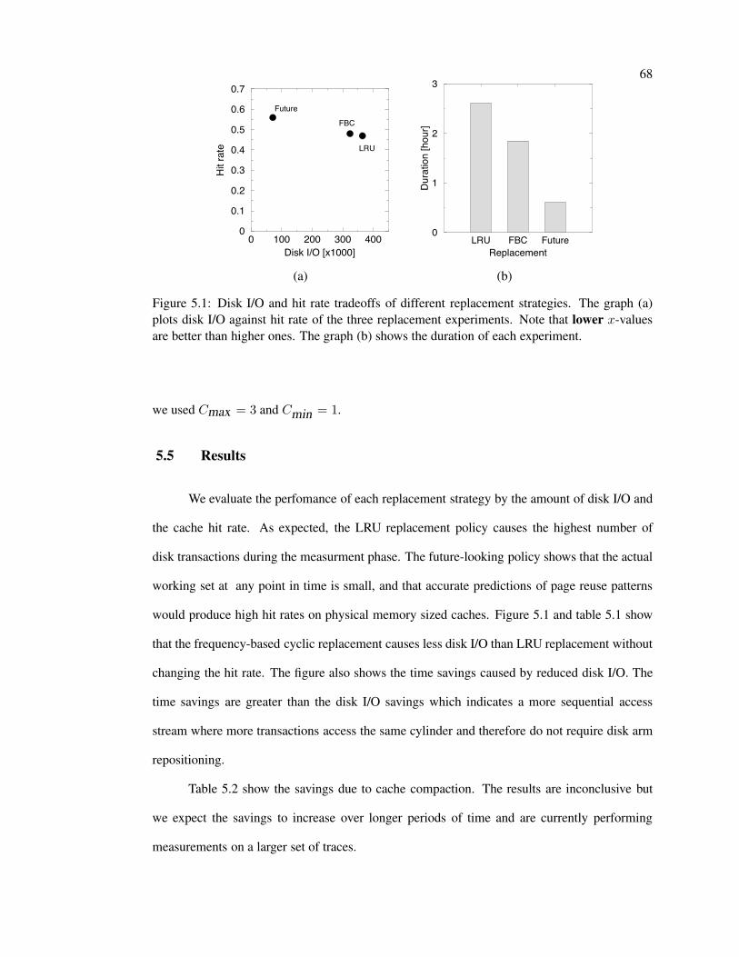
68
0 100 200 300 400Disk I/O [x1000]
0
0.1
0.2
0.3
0.4
0.5
0.6
0.7
Hit r
ate
FBCFuture
LRU
LRU FBC FutureReplacement
0
1
2
3
Dura
tion
[hou
r]
(a) (b)
Figure 5.1: Disk I/O and hit rate tradeoffs of different replacement strategies. The graph (a)plots disk I/O against hit rate of the three replacement experiments. Note that lower x-valuesare better than higher ones. The graph (b) shows the duration of each experiment.
we used Cmax = 3 and Cmin = 1.
5.5 Results
We evaluate the perfomance of each replacement strategy by the amount of disk I/O and
the cache hit rate. As expected, the LRU replacement policy causes the highest number of
disk transactions during the measurment phase. The future-looking policy shows that the actual
working set at any point in time is small, and that accurate predictions of page reuse patterns
would produce high hit rates on physical memory sized caches. Figure 5.1 and table 5.1 show
that the frequency-based cyclic replacement causes less disk I/O than LRU replacement without
changing the hit rate. The figure also shows the time savings caused by reduced disk I/O. The
time savings are greater than the disk I/O savings which indicates a more sequential access
stream where more transactions access the same cylinder and therefore do not require disk arm
repositioning.
Table 5.2 show the savings due to cache compaction. The results are inconclusive but
we expect the savings to increase over longer periods of time and are currently performing
measurements on a larger set of traces.
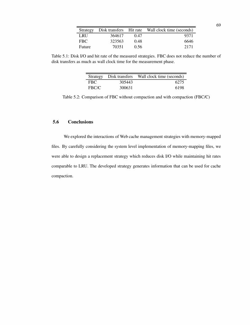
69Strategy Disk transfers Hit rate Wall clock time (seconds)LRU 364617 0.47 9371FBC 323563 0.48 6646Future 70351 0.56 2171
Table 5.1: Disk I/O and hit rate of the measured strategies. FBC does not reduce the number ofdisk transfers as much as wall clock time for the measurement phase.
Strategy Disk transfers Wall clock time (seconds)FBC 305443 6275FBC/C 300631 6198
Table 5.2: Comparison of FBC without compaction and with compaction (FBC/C)
5.6 Conclusions
We explored the interactions of Web cache management strategies with memory-mapped
files. By carefully considering the system level implementation of memory-mapping files, we
were able to design a replacement strategy which reduces disk I/O while maintaining hit rates
comparable to LRU. The developed strategy generates information that can be used for cache
compaction.
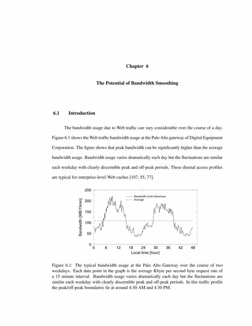
Chapter 6
The Potential of Bandwidth Smoothing
6.1 Introduction
The bandwidth usage due to Web traffic can vary considerable over the course of a day.
Figure 6.1 shows the Web traffic bandwidth usage at the Palo Alto gateway of Digital Equipment
Corporation. The figure shows that peak bandwidth can be significantly higher than the average
bandwidth usage. Bandwidth usage varies dramatically each day but the fluctuations are similar
each weekday with clearly discernible peak and off-peak periods. These diurnal access profiles
are typical for enterprise-level Web caches [107, 55, 77].
0 6 12 18 24 30 36 42 48Local time [hour]
0
50
100
150
200
250
Band
widt
h [M
B/15
min
] Bandwidth of all referencesAverage
Figure 6.1: The typical bandwidth usage at the Palo Alto Gateway over the course of twoweekdays. Each data point in the graph is the average Kbyte per second byte request rate ofa 15 minute interval. Bandwidth usage varies dramatically each day but the fluctuations aresimilar each weekday with clearly discernible peak and off-peak periods. In this traffic profilethe peak/off-peak boundaries lie at around 4:30 AM and 4:30 PM.
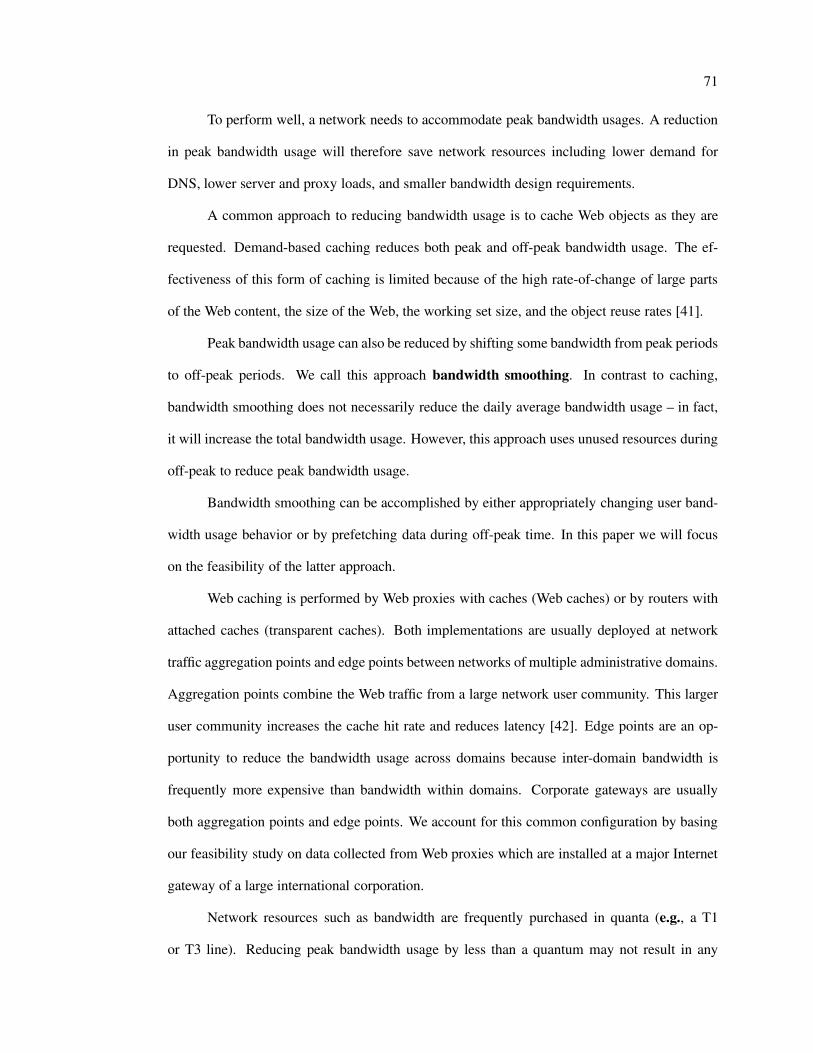
71
To perform well, a network needs to accommodate peak bandwidth usages. A reduction
in peak bandwidth usage will therefore save network resources including lower demand for
DNS, lower server and proxy loads, and smaller bandwidth design requirements.
A common approach to reducing bandwidth usage is to cache Web objects as they are
requested. Demand-based caching reduces both peak and off-peak bandwidth usage. The ef-
fectiveness of this form of caching is limited because of the high rate-of-change of large parts
of the Web content, the size of the Web, the working set size, and the object reuse rates [41].
Peak bandwidth usage can also be reduced by shifting some bandwidth from peak periods
to off-peak periods. We call this approach bandwidth smoothing. In contrast to caching,
bandwidth smoothing does not necessarily reduce the daily average bandwidth usage – in fact,
it will increase the total bandwidth usage. However, this approach uses unused resources during
off-peak to reduce peak bandwidth usage.
Bandwidth smoothing can be accomplished by either appropriately changing user band-
width usage behavior or by prefetching data during off-peak time. In this paper we will focus
on the feasibility of the latter approach.
Web caching is performed by Web proxies with caches (Web caches) or by routers with
attached caches (transparent caches). Both implementations are usually deployed at network
traffic aggregation points and edge points between networks of multiple administrative domains.
Aggregation points combine the Web traffic from a large network user community. This larger
user community increases the cache hit rate and reduces latency [42]. Edge points are an op-
portunity to reduce the bandwidth usage across domains because inter-domain bandwidth is
frequently more expensive than bandwidth within domains. Corporate gateways are usually
both aggregation points and edge points. We account for this common configuration by basing
our feasibility study on data collected from Web proxies which are installed at a major Internet
gateway of a large international corporation.
Network resources such as bandwidth are frequently purchased in quanta (e.g., a T1
or T3 line). Reducing peak bandwidth usage by less than a quantum may not result in any
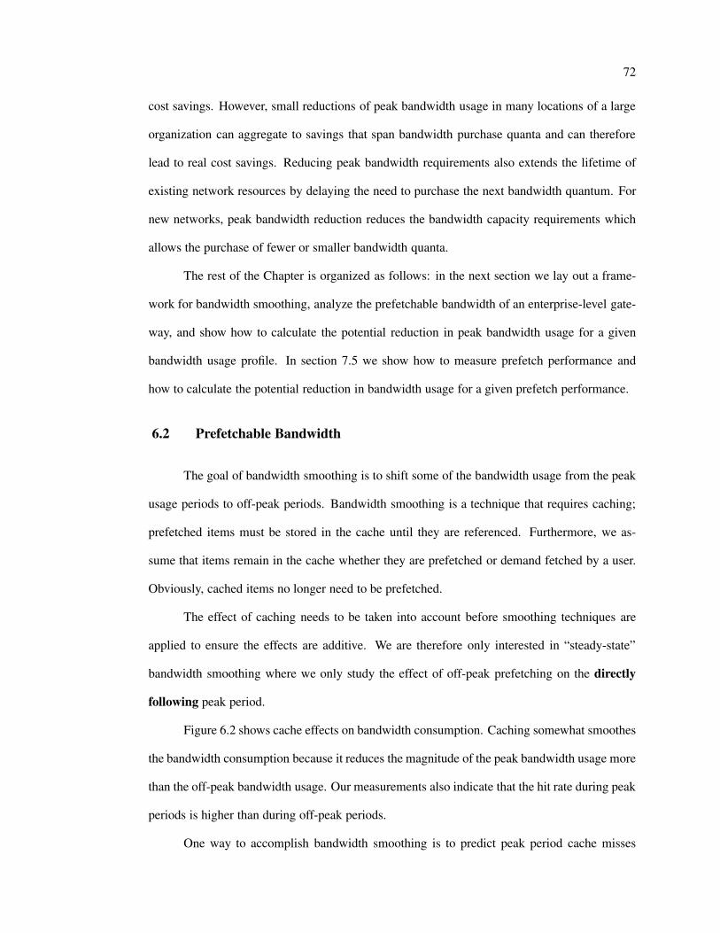
72
cost savings. However, small reductions of peak bandwidth usage in many locations of a large
organization can aggregate to savings that span bandwidth purchase quanta and can therefore
lead to real cost savings. Reducing peak bandwidth requirements also extends the lifetime of
existing network resources by delaying the need to purchase the next bandwidth quantum. For
new networks, peak bandwidth reduction reduces the bandwidth capacity requirements which
allows the purchase of fewer or smaller bandwidth quanta.
The rest of the Chapter is organized as follows: in the next section we lay out a frame-
work for bandwidth smoothing, analyze the prefetchable bandwidth of an enterprise-level gate-
way, and show how to calculate the potential reduction in peak bandwidth usage for a given
bandwidth usage profile. In section 7.5 we show how to measure prefetch performance and
how to calculate the potential reduction in bandwidth usage for a given prefetch performance.
6.2 Prefetchable Bandwidth
The goal of bandwidth smoothing is to shift some of the bandwidth usage from the peak
usage periods to off-peak periods. Bandwidth smoothing is a technique that requires caching;
prefetched items must be stored in the cache until they are referenced. Furthermore, we as-
sume that items remain in the cache whether they are prefetched or demand fetched by a user.
Obviously, cached items no longer need to be prefetched.
The effect of caching needs to be taken into account before smoothing techniques are
applied to ensure the effects are additive. We are therefore only interested in “steady-state”
bandwidth smoothing where we only study the effect of off-peak prefetching on the directly
following peak period.
Figure 6.2 shows cache effects on bandwidth consumption. Caching somewhat smoothes
the bandwidth consumption because it reduces the magnitude of the peak bandwidth usage more
than the off-peak bandwidth usage. Our measurements also indicate that the hit rate during peak
periods is higher than during off-peak periods.
One way to accomplish bandwidth smoothing is to predict peak period cache misses
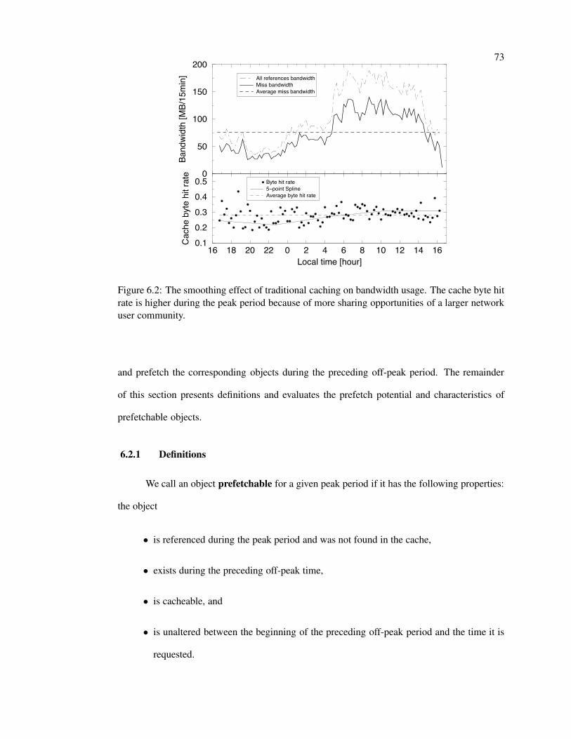
73
0
50
100
150
200
Band
widt
h [M
B/15
min
] All references bandwidthMiss bandwidthAverage miss bandwidth
16 18 20 22 0 2 4 6 8 10 12 14 16Local time [hour]
0.10.20.30.40.5
Cach
e by
te h
it ra
teByte hit rate5−point SplineAverage byte hit rate
Figure 6.2: The smoothing effect of traditional caching on bandwidth usage. The cache byte hitrate is higher during the peak period because of more sharing opportunities of a larger networkuser community.
and prefetch the corresponding objects during the preceding off-peak period. The remainder
of this section presents definitions and evaluates the prefetch potential and characteristics of
prefetchable objects.
6.2.1 Definitions
We call an object prefetchable for a given peak period if it has the following properties:
the object
• is referenced during the peak period and was not found in the cache,
• exists during the preceding off-peak time,
• is cacheable, and
• is unaltered between the beginning of the preceding off-peak period and the time it is
requested.
74
If an object fails to meet any of these conditions for a given peak period we call it
non-prefetchable for that peak period. Because of the first condition a non-prefetchable ob-
ject during one peak period can be a prefetchable object during another peak period. Non-
prefetchable objects which meet all prefetchability conditions except the first are called no-
miss-prefetchable objects.
The combined size of all prefetchable objects of a given peak period is the prefetchable
bandwidth. There are three disjoint kinds of prefetchable objects, depending on the Web access
history of the aggregated network user community:
• Seen prefetchable objects have names which were previously referenced. These are
either revalidation misses (caused by stale data) or capacity misses (caused by finite-
capacity caches).
• Seen-server prefetchable objects are referenced for the first time, but they are served
from previously accessed Web servers. These are compulsory misses because they
have not been seen before.
• The names and servers of unseen-server prefetchable objects were unknown prior
to the current reference. Neither the object nor the server were previously accessed.
These are also compulsory misses because the data has not been seen before
We distinguish seen-server prefetchable and unseen-server prefetchable objects be-
cause predicting the latter kind of objects is more difficult: the proxy access history offers no
information about the existence of unseen servers.
6.2.2 Experimental Measurement and Evaluation Environment
In order to estimate the prefetchable bandwidth for bandwidth smoothing we analyzed
the Digital WRL HTTP proxy request traces [69]. The instrumented HTTP proxies were in-
stalled at a gateway that connects a large international corporate intranet to the Internet. The
75
traces were “sanitized” to protect individual privacy and other sensitive information such as in-
dividual Web site access counts. As a consequence, each Web server host, path, query, client,
and URL (combination of host, path, and query) are encoded by identity preserving, unique
numbers. The traces cover the days from August 29th through September 22nd, 1996 and con-
sist of over 22 million requests.
For the sake of simplicity we divided bandwidth usage into off-peak periods starting
at 4:30 PM and ending at 4:30 AM each weekday, and peak periods starting at 4:30 AM and
ending at 4:30 PM each weekday (see figure 6.1). We analyzed the HTTP traffic to obtain object
age information in order to identify prefetchable objects.
To identify misses in the Digital WRL trace (which was generated by a cacheless Web
proxy), we assumed (1) a cache of infinite size, (2) a cache hit is represented by a re-reference
of an object with the same modification date as the previous reference1, and (3) the cache never
serves a stale object. From this cache model we determine the list of objects and the miss
bandwidth for peak and off-peak periods.
To preclude any cache cold-start effects on our measurements we applied this model for
at least two days worth of trace data before taking any bandwidth measurements.
6.2.3 Prefetchable Bandwidth Analysis
Figure 6.3 shows the composition of the miss bandwidth during a typical weekday peak
period of the Digital trace out of an infinite cache. About 40% of the miss bandwidth is prefetch-
able.
Almost all the prefetchable bandwidth consists of seen-server prefetchable objects. The
other prefetchable components (seen prefetchable and unseen-server prefetchable objects)
are negligible. With a fixed size cache the number of seen prefetchable objects would increase
through capacity misses. Unseen-server prefetchable objects are entirely workload dependent1 The modification date must be non-zero. By convention a modification date of zero is used for dynamic and
non-cacheable objects, i.e. these objects always miss in the cache. Some researchers use modification date and sizeto differentiate objects [88]. However, we are not aware of any Web caches which do not determine object stalenesssolely based on object age.
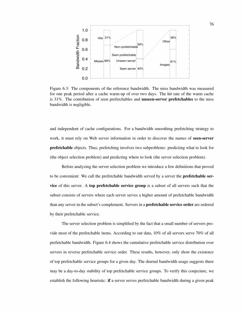
76
0.0
0.2
0.4
0.6
0.8
1.0
Band
widt
h Fr
actio
n
Hits
Misses
Non−prefetchable
Unseen server
Seen prefetchable
Seen serverImages
Other31%
69%
59%
40%
61%
39%
Figure 6.3: The components of the reference bandwidth. The miss bandwidth was measuredfor one peak period after a cache warm-up of over two days. The hit rate of the warm cacheis 31%. The contribution of seen prefetchables and unseen-server prefetchables to the missbandwidth is negligible.
and independent of cache configurations. For a bandwidth smoothing prefetching strategy to
work, it must rely on Web server information in order to discover the names of seen-server
prefetchable objects. Thus, prefetching involves two subproblems: predicting what to look for
(the object selection problem) and predicting where to look (the server selection problem).
Before analyzing the server selection problem we introduce a few definitions that proved
to be convenient: We call the prefetchable bandwidth served by a server the prefetchable ser-
vice of this server. A top prefetchable service group is a subset of all servers such that the
subset consists of servers where each server serves a higher amount of prefetchable bandwidth
than any server in the subset’s complement. Servers in a prefetchable service order are ordered
by their prefetchable service.
The server selection problem is simplified by the fact that a small number of servers pro-
vide most of the prefetchable items. According to our data, 10% of all servers serve 70% of all
prefetchable bandwidth. Figure 6.4 shows the cumulative prefetchable service distribution over
servers in reverse prefetchable service order. These results, however, only show the existence
of top prefetchable service groups for a given day. The diurnal bandwidth usage suggests there
may be a day-to-day stability of top prefetchable service groups. To verify this conjecture, we
establish the following heuristic: if a server serves prefetchable bandwidth during a given peak
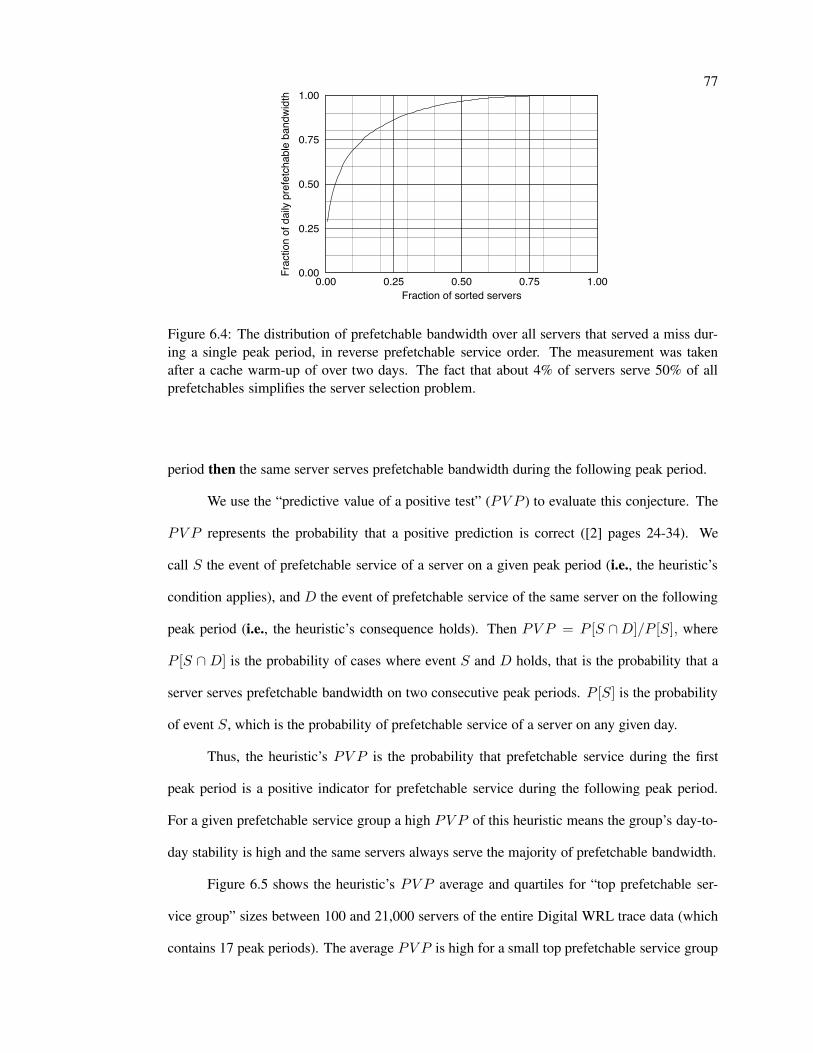
77
0.00 0.25 0.50 0.75 1.00Fraction of sorted servers
0.00
0.25
0.50
0.75
1.00
Frac
tion
of d
aily
pref
etch
able
ban
dwid
th
Figure 6.4: The distribution of prefetchable bandwidth over all servers that served a miss dur-ing a single peak period, in reverse prefetchable service order. The measurement was takenafter a cache warm-up of over two days. The fact that about 4% of servers serve 50% of allprefetchables simplifies the server selection problem.
period then the same server serves prefetchable bandwidth during the following peak period.
We use the “predictive value of a positive test” (PV P ) to evaluate this conjecture. The
PV P represents the probability that a positive prediction is correct ([2] pages 24-34). We
call S the event of prefetchable service of a server on a given peak period (i.e., the heuristic’s
condition applies), and D the event of prefetchable service of the same server on the following
peak period (i.e., the heuristic’s consequence holds). Then PV P = P [S ∩D]/P [S], where
P [S ∩ D] is the probability of cases where event S and D holds, that is the probability that a
server serves prefetchable bandwidth on two consecutive peak periods. P [S] is the probability
of event S, which is the probability of prefetchable service of a server on any given day.
Thus, the heuristic’s PV P is the probability that prefetchable service during the first
peak period is a positive indicator for prefetchable service during the following peak period.
For a given prefetchable service group a high PV P of this heuristic means the group’s day-to-
day stability is high and the same servers always serve the majority of prefetchable bandwidth.
Figure 6.5 shows the heuristic’s PV P average and quartiles for “top prefetchable ser-
vice group” sizes between 100 and 21,000 servers of the entire Digital WRL trace data (which
contains 17 peak periods). The average PV P is high for a small top prefetchable service group
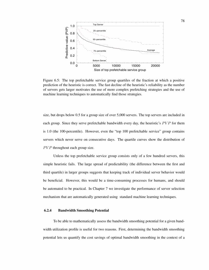
78
0 5000 10000 15000 20000Size of top prefetchable service group
0.0
0.2
0.4
0.6
0.8
1.0
Pred
ictive
val
ue (P
VP)
50−percentile
75−percentile
25−percentile
Top Server
Bottom Server
Average
Figure 6.5: The top prefetchable service group quartiles of the fraction at which a positiveprediction of the heuristic is correct. The fast decline of the heuristic’s reliability as the numberof servers gets larger motivates the use of more complex prefetching strategies and the use ofmachine learning techniques to automatically find those strategies.
size, but drops below 0.5 for a group size of over 5,000 servers. The top servers are included in
each group. Since they serve prefetchable bandwidth every day, the heuristic’s PV P for them
is 1.0 (the 100-percentile). However, even the “top 100 prefetchable service” group contains
servers which never serve on consecutive days. The quartile curves show the distribution of
PV P throughout each group size.
Unless the top prefetchable service group consists only of a few hundred servers, this
simple heuristic fails. The large spread of predictability (the difference between the first and
third quartile) in larger groups suggests that keeping track of individual server behavior would
be beneficial. However, this would be a time-consuming processes for humans, and should
be automated to be practical. In Chapter 7 we investigate the performance of server selection
mechanism that are automatically generated using standard machine learning techniques.
6.2.4 Bandwidth Smoothing Potential
To be able to mathematically assess the bandwidth smoothing potential for a given band-
width utilization profile is useful for two reasons. First, determining the bandwidth smoothing
potential lets us quantify the cost savings of optimal bandwidth smoothing in the context of a
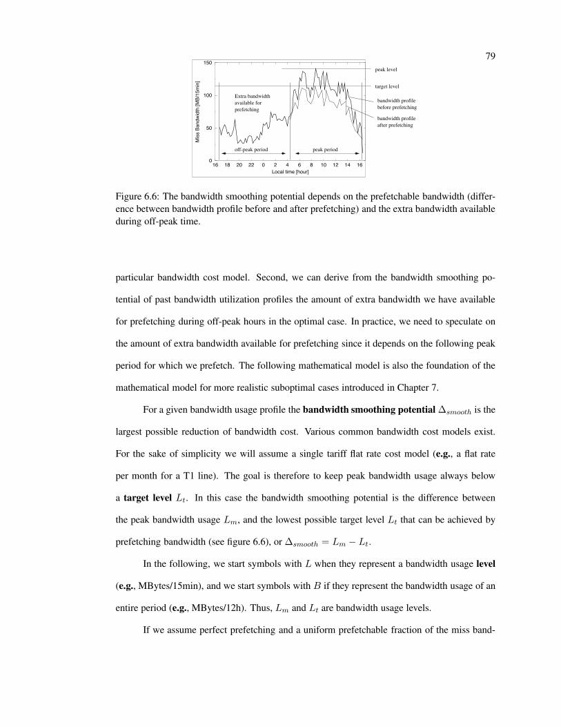
79
16 18 20 22 0 2 4 6 8 10 12 14 16Local time [hour]
0
50
100
150
Miss
Ban
dwid
th [M
B/15
min
]
peak level
off-peak period peak period
target level
Extra bandwidthavailable for prefetching
bandwidth profilebefore prefetching
bandwidth profileafter prefetching
Figure 6.6: The bandwidth smoothing potential depends on the prefetchable bandwidth (differ-ence between bandwidth profile before and after prefetching) and the extra bandwidth availableduring off-peak time.
particular bandwidth cost model. Second, we can derive from the bandwidth smoothing po-
tential of past bandwidth utilization profiles the amount of extra bandwidth we have available
for prefetching during off-peak hours in the optimal case. In practice, we need to speculate on
the amount of extra bandwidth available for prefetching since it depends on the following peak
period for which we prefetch. The following mathematical model is also the foundation of the
mathematical model for more realistic suboptimal cases introduced in Chapter 7.
For a given bandwidth usage profile the bandwidth smoothing potential ∆smooth is the
largest possible reduction of bandwidth cost. Various common bandwidth cost models exist.
For the sake of simplicity we will assume a single tariff flat rate cost model (e.g., a flat rate
per month for a T1 line). The goal is therefore to keep peak bandwidth usage always below
a target level Lt. In this case the bandwidth smoothing potential is the difference between
the peak bandwidth usage Lm, and the lowest possible target level Lt that can be achieved by
prefetching bandwidth (see figure 6.6), or ∆smooth = Lm − Lt.
In the following, we start symbols with L when they represent a bandwidth usage level
(e.g., MBytes/15min), and we start symbols with B if they represent the bandwidth usage of an
entire period (e.g., MBytes/12h). Thus, Lm and Lt are bandwidth usage levels.
If we assume perfect prefetching and a uniform prefetchable fraction of the miss band-
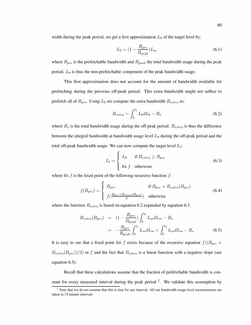
80
width during the peak period, we get a first approximation L0 of the target level by:
L0 = (1− Bpre
Bpeak)Lm (6.1)
where Bpre is the prefetchable bandwidth and Bpeak the total bandwidth usage during the peak
period. L0 is thus the non-prefetchable component of the peak bandwidth usage.
This first approximation does not account for the amount of bandwidth available for
prefetching during the previous off-peak period. This extra bandwidth might not suffice to
prefetch all of Bpre. Using L0 we compute the extra bandwidth Bextra as:
Bextra =∫ t0
0L0dL0 −Bo (6.2)
where Bo is the total bandwidth usage during the off-peak period. Bextra is thus the difference
between the integral bandwidth at bandwidth usage level L0 during the off-peak period and the
total off-peak bandwidth usage. We can now compute the target level Lt:
Lt =
L0 if Bextra ≥ Bpre
fix f otherwise(6.3)
where fix f is the fixed point of the following recursive function f :
f(Bpre) =
Bpre if Bpre = Bextra(Bpre)
f(Bpre+Bextra(Bpre)2 ) otherwise
(6.4)
where the function Bextra is based on equation 6.2 expanded by equation 6.1:
Bextra(Bpre) = (1− Bpre
Bpeak)∫ t0
0LmdLm −Bo
= − Bpre
Bpeak
∫ t0
0LmdLm +
∫ t0
0LmdLm −Bo (6.5)
It is easy to see that a fixed point for f exists because of the recursive equation f((Bpre +
Bextra(Bpre))/2) in f and the fact that Bextra is a linear function with a negative slope (see
equation 6.5).
Recall that these calculations assume that the fraction of prefetchable bandwidth is con-
stant for every measured interval during the peak period 2. We validate this assumption by2 Note that we do not assume that this is true for any interval. All our bandwidth usage level measurements are
taken in 15 minute intervals
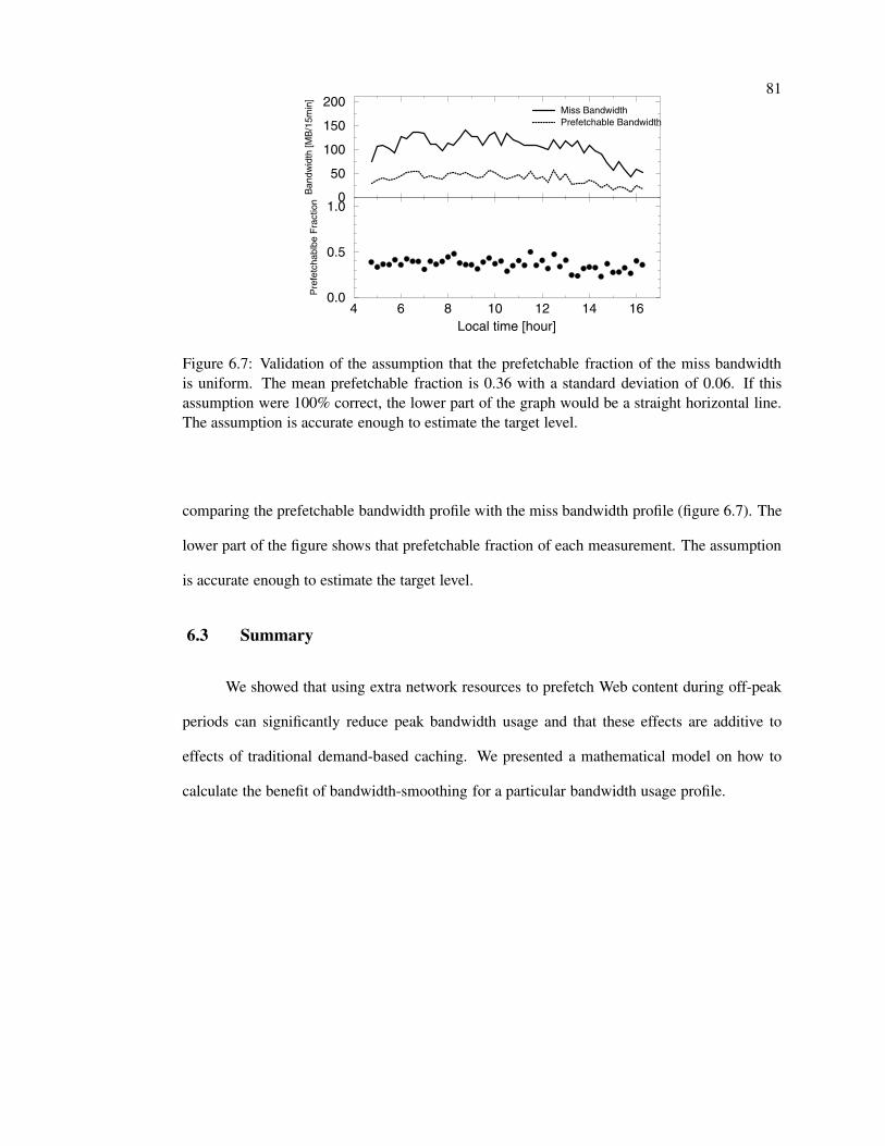
81
0
50
100
150
200
Ban
dwid
th [M
B/1
5min
]
Miss BandwidthPrefetchable Bandwidth
4 6 8 10 12 14 16Local time [hour]
0.0
0.5
1.0
Pre
fetc
habl
be F
ract
ion
Figure 6.7: Validation of the assumption that the prefetchable fraction of the miss bandwidthis uniform. The mean prefetchable fraction is 0.36 with a standard deviation of 0.06. If thisassumption were 100% correct, the lower part of the graph would be a straight horizontal line.The assumption is accurate enough to estimate the target level.
comparing the prefetchable bandwidth profile with the miss bandwidth profile (figure 6.7). The
lower part of the figure shows that prefetchable fraction of each measurement. The assumption
is accurate enough to estimate the target level.
6.3 Summary
We showed that using extra network resources to prefetch Web content during off-peak
periods can significantly reduce peak bandwidth usage and that these effects are additive to
effects of traditional demand-based caching. We presented a mathematical model on how to
calculate the benefit of bandwidth-smoothing for a particular bandwidth usage profile.

Chapter 7
Generating Prefetch Strategies using Machine Learning
7.1 Introduction
As we have seen in Chapter 6, the performance of simple prefetch strategies is unsatis-
fying. More complex strategies are necessary to achieve higher performance. However, more
complex strategies will likely be more specific to the particular traffic for which they are de-
signed for. Furthermore, the particular traffic is changing over time, degrading the performance
of complex prefetch strategies over time. Thus, hand-coding a prefetch strategy might be too
slow and tedious of a process to be feasible.
In this Chapter we demonstrate and discuss the performance of machine learning tech-
niques to automatically and quickly develop prefetch strategies. First we give an overview
of machine learning techniques and give an introduction of the particular technique we chose.
Then we show how we generate prefetch strategies and finally we evaluate the performance of
generated strategies and analyze their composition.
7.2 Machine Learning
There are many approaches to machine learning. We used an approach called supervised
learning, where the learning algorithm is given a set of input-output pairs (labeled data). The
input describes the information available for making the decision and the output describes the
correct decision [38]. As we demonstrate below, trace data of Web proxy servers and content
on the Web provide a wealth of labeled data.
83
The result of a learning task is a classification model (also called a classifier) which
allows the classification of unseen data below a certain error rate. For generating prefetch
strategies we use a tool called RIPPER [28] which efficiently produces and evaluates a classifier
in form of a propositional rule set and which is freely available for non-commercial use at [29].
To illustrate what RIPPER does we use a simple learning task from the golf playing
domain. First we need to declare the values of attributes and classes:
Play, ’No Play’.
outlook: sunny, overcast, rain.
temperature: continuous.
humidity: continuous.
windy: true, false.
The first line defines the possible class values (either “Play” or “No Play”). The last four lines
define the name and possible values of each attribute that characterizes each training case. Each
line in the following training data shows an example of when to play or not to play golf. The
first four values correspond to the four attribute definition above, and the last value marks the
classification of the example.
sunny, 85, 85, false, ’No Play’.
sunny, 80, 90, true, ’No Play’.
overcast, 83, 78, false, Play.
rain, 70, 96, false, Play.
rain, 68, 80, false, Play.
rain, 65, 70, true, ’No Play’.
overcast, 64, 65, true, Play.
sunny, 72, 95, false, ’No Play’.
sunny, 69, 70, false, Play.
rain, 75, 80, false, Play.
84
sunny, 75, 70, true, Play.
overcast, 72, 90, true, Play.
overcast, 81, 75, false, Play.
rain, 71, 80, true, ’No Play’.
From this data RIPPER constructs a classifier in the form of three rules: two rules on when not
to play and one rule that defines the default value as “Play”. The first rule means,“if it is windy
and rain is to be expected, do not play golf,” and the second, “if the humidity is 85% or higher
and the outlook is sunny, do not play golf.”
’No Play’ :- windy=true, outlook=rain (2/0).
’No Play’ :- humidity>=85, outlook=sunny (3/0).
default Play (9/0).
The golf data set is a coherent data set, i.e. none of the examples contradict each other. This
is reflected in the parenthesized values after each rule which indicate the number of examples
which support the rule and the number of examples which do not match the rule. In a coherent
data set the latter is always zero. The real strength of RIPPER is its ability to deal with incoherent
data sets with contradicting examples. In this case RIPPER attempts to identify a classifier with
a low error rate.
RIPPER also supports the construction of ensembles of classifiers. An ensemble of
classifiers is a set of classifiers whose individual decisions are combined in some way, usually
by weighted voting (see [39] for an overview). Our results include performance data using
an ensemble construction algorithm called ADABOOST [52, 51]. The technique is also called
boosting and works roughly like this: Each classifier is constructed using a “weak learner”
such as RIPPER. The difference between the individual classifiers is that they are trained on
increasingly more difficult learning problems. The first classifier is learned by the original
training data. The next learning problem is constructed by adding weight to the examples which
are misclassified by the first classifier. This more difficult learning problem is used to train the

85
next classifier. The examples misclassified by the second classifier receive additional weight in
the next learning problem, and so on.
7.3 Training
In order to find a prefetch strategy, one has to find training data consisting of positive evi-
dence, i.e. examples of objects that should be prefetched, and negative evidence, i.e. examples
of objects that should not be prefetched.
Access log data from Web proxy servers provides positive evidence because it includes
sufficient information to identify prefetchable objects (in the strict sense of our definition of
prefetchable objects). Negative evidence consists of objects that do not meet all prefetchability
conditions. Access log data provides some negative evidence as it includes all objects that are
missed during a peak period but either didn’t exist during the preceding off-peak time, were
not cacheable, or were modified between the beginning of the preceding off-peak period and
the time it was requested. However, access log data does not include any evidence of no-miss-
prefetchables, objects that meet all prefetchability conditions except they are not missed during
a peak period. This information is only available from a content summary of Web servers which
include the name and other attributes about each potentially prefetchable object.
There are multiple ways to acquire this information which differ in their impact on band-
width consumption and their requirements on local services. For example, if the local site also
runs a large search engine, the negative evidence can be derived from the search engine index as
long as the search index contains information about textual as well as non-textual objects (see
for example [16]). This approach has very little impact on bandwidth consumption. If no local
search engine is available, a remote search engine could offer a service that allows querying
for a very compact representation of the names and attributes of objects with certain properties.
Finally, servers themselves could provide such a querying service in some well-known manner.
86
7.4 Training and Testing Methodology
We collected access log data of 14 days of full gateway traffic at Digital WRL (Monday,
5/18/1998 - Sunday, 5/31/1998). Near the end of the 14 day period, during Friday, 5/29/1998,
we identified the top 320 prefetchable service group which serves about 45% of the total
prefetchable bandwidth during the 11 day period prior to Friday. Having none of the above
services available for efficiently acquiring Web server content information, we used a “Web
robot” to scan these 320 servers during the weekend (5/30-31/1998). The resulting scan con-
tains information on 1,935,086 objects. Limited resources prevented us from scanning more
than 320 servers and because of time constraints we were unable to completely scan these 320
servers. To estimate the relative size of the scan data sample, we assume that prefetchable ob-
jects are uniformly distributed in any scan data. Since we know the amount of prefetchable
bandwidth from the access log data we can then approximate the scan data sample size by the
fraction of the prefetchable bandwidth contained in the scan data. According to this approxi-
mation our scan data sample size is about 22% of the size of the entire content of the scanned
servers.
For the positive evidence we identified and encoded each prefetchable object in the ac-
cess log by six attributes: (1) age, (2) MIME type, (3) size, (4) server name, (5) top level
domain, (6) the label that marks this entry as prefetchable, and (7) a weight proportional to the
size. The first three attributes train object selection, the fourth and fifth attribute train server se-
lection, and the weight represents the relative significance of an entry to the overall bandwidth
consumption.
For the negative evidence we collected each day’s no-miss-prefetchable objects from the
scan data. Recall that no-miss-prefetchable objects are objects that meet all prefetchability con-
ditions as described in section 6.2.1 except the first condition, i.e. the object is not missed during
the peak period of the current day. Each no-miss-prefetchable object is encoded and weighted
in the same way as prefetchable objects except that the entry is labeled as non-prefetchable.
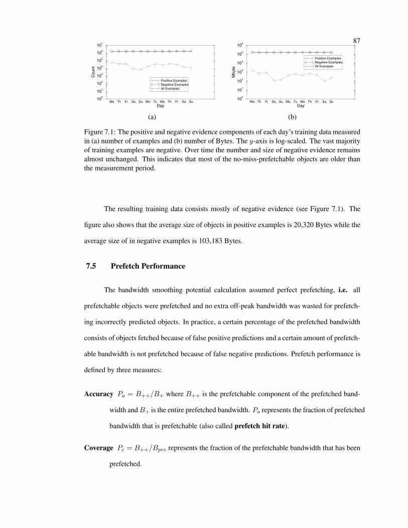
87
We Th Fr Sa Su Mo Tu We Th Fr Sa SuDay
100
101
102
103
104
105
106
107
Coun
t
Positive ExamplesNegative ExamplesAll Examples
We Th Fr Sa Su Mo Tu We Th Fr Sa SuDay
100
101
102
103
104
105
106
Mby
te
Positive ExamplesNegative ExamplesAll Examples
(a) (b)
Figure 7.1: The positive and negative evidence components of each day’s training data measuredin (a) number of examples and (b) number of Bytes. The y-axis is log-scaled. The vast majorityof training examples are negative. Over time the number and size of negative evidence remainsalmost unchanged. This indicates that most of the no-miss-prefetchable objects are older thanthe measurement period.
The resulting training data consists mostly of negative evidence (see Figure 7.1). The
figure also shows that the average size of objects in positive examples is 20,320 Bytes while the
average size of in negative examples is 103,183 Bytes.
7.5 Prefetch Performance
The bandwidth smoothing potential calculation assumed perfect prefetching, i.e. all
prefetchable objects were prefetched and no extra off-peak bandwidth was wasted for prefetch-
ing incorrectly predicted objects. In practice, a certain percentage of the prefetched bandwidth
consists of objects fetched because of false positive predictions and a certain amount of prefetch-
able bandwidth is not prefetched because of false negative predictions. Prefetch performance is
defined by three measures:
Accuracy Pa = B++/B+ where B++ is the prefetchable component of the prefetched band-
width and B+ is the entire prefetched bandwidth. Pa represents the fraction of prefetched
bandwidth that is prefetchable (also called prefetch hit rate).
Coverage Pc = B++/Bpre represents the fraction of the prefetchable bandwidth that has been
prefetched.
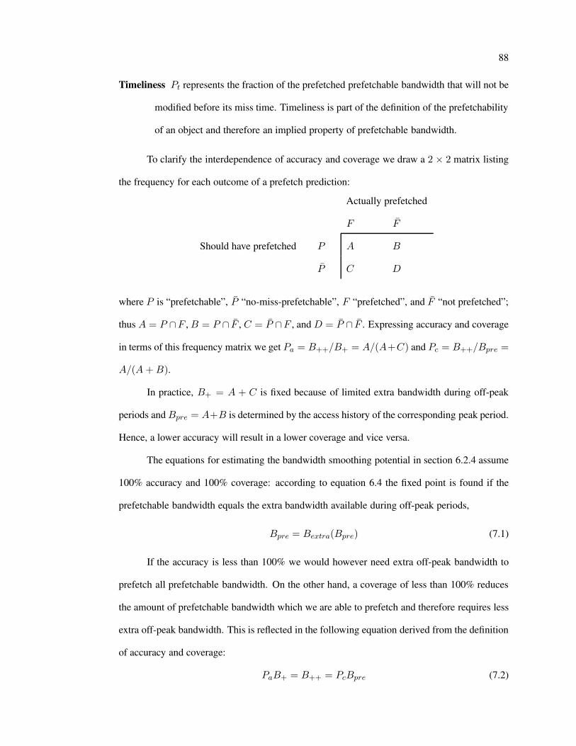
88
Timeliness Pt represents the fraction of the prefetched prefetchable bandwidth that will not be
modified before its miss time. Timeliness is part of the definition of the prefetchability
of an object and therefore an implied property of prefetchable bandwidth.
To clarify the interdependence of accuracy and coverage we draw a 2 × 2 matrix listing
the frequency for each outcome of a prefetch prediction:
Actually prefetched
F F
Should have prefetched P A B
P C D
where P is “prefetchable”, P “no-miss-prefetchable”, F “prefetched”, and F “not prefetched”;
thus A = P ∩F , B = P ∩ F , C = P ∩F , and D = P ∩ F . Expressing accuracy and coverage
in terms of this frequency matrix we get Pa = B++/B+ = A/(A+C) and Pc = B++/Bpre =
A/(A+B).
In practice, B+ = A + C is fixed because of limited extra bandwidth during off-peak
periods and Bpre = A+B is determined by the access history of the corresponding peak period.
Hence, a lower accuracy will result in a lower coverage and vice versa.
The equations for estimating the bandwidth smoothing potential in section 6.2.4 assume
100% accuracy and 100% coverage: according to equation 6.4 the fixed point is found if the
prefetchable bandwidth equals the extra bandwidth available during off-peak periods,
Bpre = Bextra(Bpre) (7.1)
If the accuracy is less than 100% we would however need extra off-peak bandwidth to
prefetch all prefetchable bandwidth. On the other hand, a coverage of less than 100% reduces
the amount of prefetchable bandwidth which we are able to prefetch and therefore requires less
extra off-peak bandwidth. This is reflected in the following equation derived from the definition
of accuracy and coverage:
PaB+ = B++ = PcBpre (7.2)
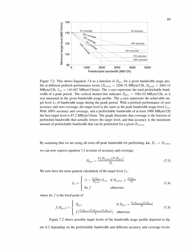
89
0 1000 2000 3000 4000 5000Prefetchable bandwidth [MB/12h]
80
100
120
140
160
Min
imum
targ
et le
vel [
MB/
15m
in]
0% accuracy
25% accuracy
50% accuracy
75% accuracy100% accuracy
0% coverage25% coverage50% coverage75% coverage
100% coverage
Figure 7.2: This shows Equation 7.4 as a function of Bpre for a given bandwidth usage pro-file at different prefetch performance levels (Bextra = 2296.78 MByte/12h, Bpeak = 4968.19MByte/12h, Lm = 140.667 MByte/15min). The x-axis represents the total prefetchable band-width of a peak period. The vertical dashed line indicates Bpre = 1965.93 MByte/12h, as itwas measured in the given bandwidth usage profile. The y-axis represents the achievable tar-get level Lt of bandwidth usage during the peark period. With a prefetch performance of zeroaccuracy and zero coverage, the target level is the same as the peak bandwidth usage level Lm.With 100% accuracy and coverage, and a prefetchable bandwidth of at least 1900 MByte/12hthe best target level is 87.2 MByte/15min. The graph illustrates that coverage is the fraction ofprefetched bandwidth that actually lowers the target level, and that accuracy is the maximumamount of prefetchable bandwidth that can be prefetched for a given Bextra.
By assuming that we are using all extra off-peak bandwidth for prefetching, i.e. B+ = Bextra
we can now express equation 7.1 in terms of accuracy and coverage:
Bpre =PaBextra(PcBpre)
Pc(7.3)
We now have the more general calculation of the target level Lt:
Lt =
(1− PcBpre
Bpeak)Lm if Bextra ≥ PcBpre
Pa
fix f otherwise(7.4)
where fix f is the fixed point of
f(Bpre) =
Bpre if Bpre =PaBextra(PcBpre)
Pc
f(PcBpre+PaBextra(PcBpre)2 ) otherwise
(7.5)
Figure 7.2 shows possible target levels of the bandwidth usage profile depicted in fig-
ure 6.2 depending on the prefetchable bandwidth and different accuracy and coverage levels.
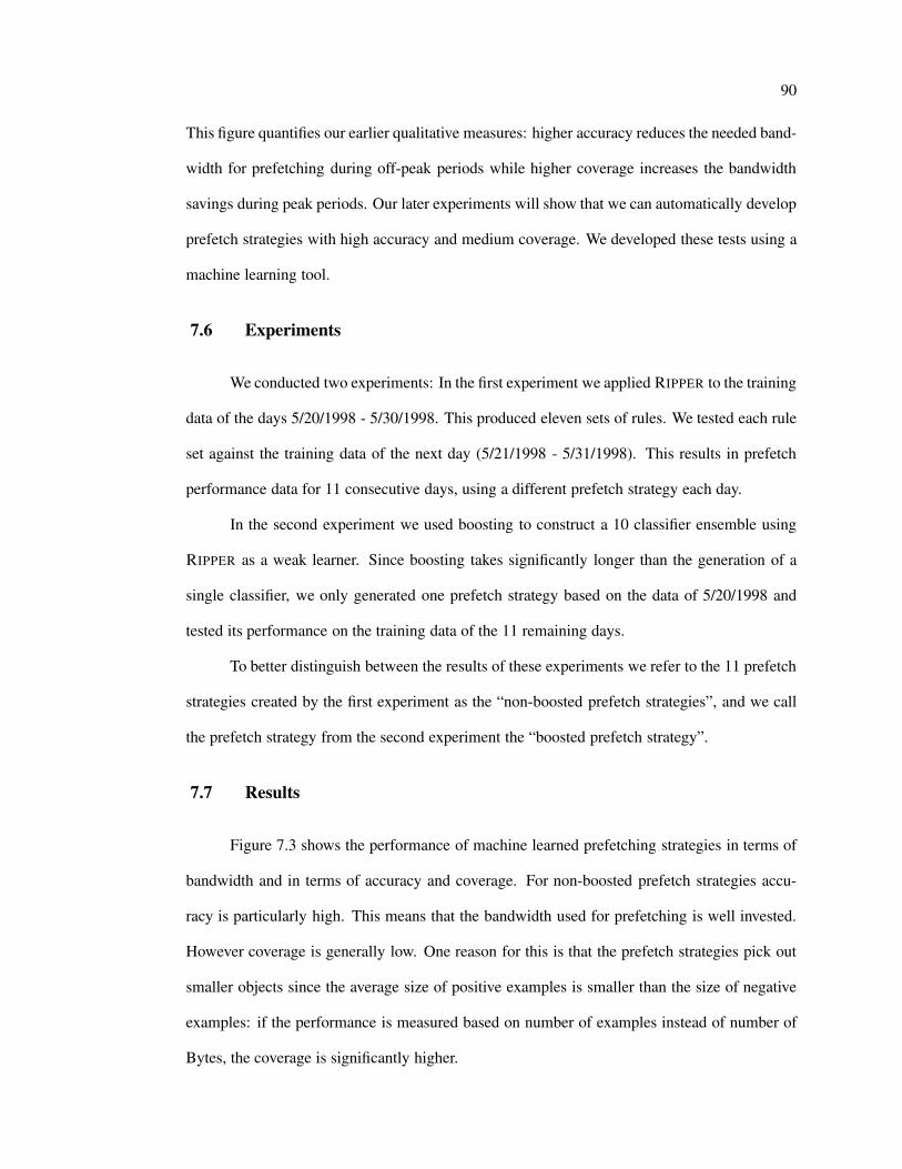
90
This figure quantifies our earlier qualitative measures: higher accuracy reduces the needed band-
width for prefetching during off-peak periods while higher coverage increases the bandwidth
savings during peak periods. Our later experiments will show that we can automatically develop
prefetch strategies with high accuracy and medium coverage. We developed these tests using a
machine learning tool.
7.6 Experiments
We conducted two experiments: In the first experiment we applied RIPPER to the training
data of the days 5/20/1998 - 5/30/1998. This produced eleven sets of rules. We tested each rule
set against the training data of the next day (5/21/1998 - 5/31/1998). This results in prefetch
performance data for 11 consecutive days, using a different prefetch strategy each day.
In the second experiment we used boosting to construct a 10 classifier ensemble using
RIPPER as a weak learner. Since boosting takes significantly longer than the generation of a
single classifier, we only generated one prefetch strategy based on the data of 5/20/1998 and
tested its performance on the training data of the 11 remaining days.
To better distinguish between the results of these experiments we refer to the 11 prefetch
strategies created by the first experiment as the “non-boosted prefetch strategies”, and we call
the prefetch strategy from the second experiment the “boosted prefetch strategy”.
7.7 Results
Figure 7.3 shows the performance of machine learned prefetching strategies in terms of
bandwidth and in terms of accuracy and coverage. For non-boosted prefetch strategies accu-
racy is particularly high. This means that the bandwidth used for prefetching is well invested.
However coverage is generally low. One reason for this is that the prefetch strategies pick out
smaller objects since the average size of positive examples is smaller than the size of negative
examples: if the performance is measured based on number of examples instead of number of
Bytes, the coverage is significantly higher.
91
Th Fr Sa Su Mo Tu We Th Fr Sa SuDay
0
200
400
600
800
1000
MBy
te /
12h
Prefetchable BandwidthPrefetched BandwidthPrefetched Prefetchables
Th Fr Sa Su Mo Tu We Th Fr Sa SuDay
0
0.2
0.4
0.6
0.8
1
Ratio Accuracy
Coverage
(a) (b)
Th Fr Sa Su Mo Tu We Th Fr Sa SuDay
0
200
400
600
800
1000
MBy
te /
12h
Prefetchable BandwidthPrefetched BandwidthPrefetched Prefetchables
Th Fr Sa Su Mo Tu We Th Fr Sa SuDay
0
0.2
0.4
0.6
0.8
1
Ratio Accuracy
Coverage
(c) (d)
Figure 7.3: Graphs (a) and (b) show the performance of non-boosted prefetch strategies, eachone trained on the day previous to the indicated day. Graphs (c) and (d) show the performanceof the boosted prefetch strategy which was learned on the Wednesday prior to the first Thursday.“Prefetchable bandwidth” represents the total prefetchable bandwidth during the peak period ofthe indicated day. “Prefetched bandwidth” shows the total bandwidth prefetched during the off-peak period prior to the peak period of the indicated day. “Prefetched prefetchables” shows thetotal amount of bandwidth saved due to prefetching. The performance on Saturday and Tuesday(Monday was Memorial Day) is weak because of the different traffic pattern of week days andweekend/holidays. In terms of saved bandwidth the boosted prefetch strategy out-performs allnon-boosted strategies but shows lower accuracy, particularly during the weekends.
Notice that the first weekend is Memorial Day weekend. HTTP traffic patterns during
weekends and holidays are different from traffic patterns during work days. Therefore, Friday
provides poor training data for Saturday, and Memorial Monday provides poor training data for
Tuesday. This is reflected by relatively low accuracy on Saturday and Tuesday. A better strategy
would be to use the previous Sunday as training day for a Saturday, and to use previous Friday
as a training day for the first week day, in this case Tuesday.
The performance of the boosted prefetch strategy is particularly high on the first Thurs-
day and Friday because of the proximity to the day of training. In terms of saved bandwidth
the boosted prefetch strategy out-performs all non-boosted strategies but shows lower accuracy,
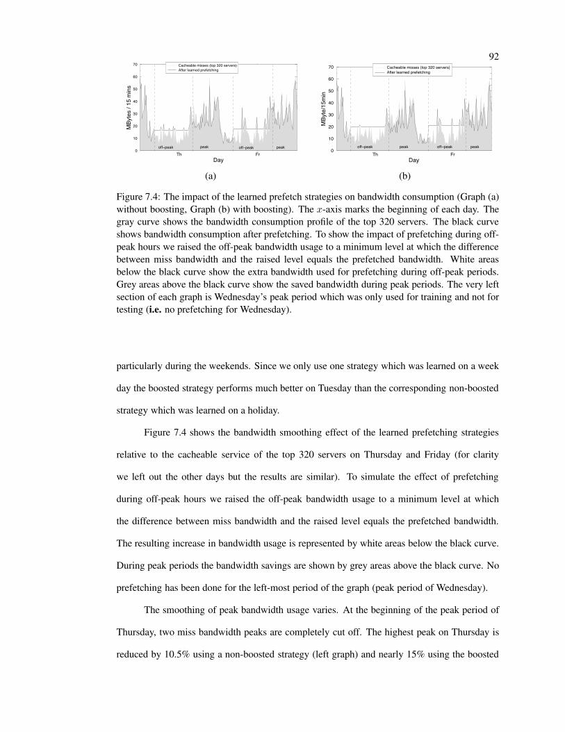
92
Th FrDay
0
10
20
30
40
50
60
70
MBy
tes
/ 15
min
s
Cacheable misses (top 320 servers)After learned prefetching
off−peak peak off−peak peak
Th FrDay
0
10
20
30
40
50
60
70
MBy
te/1
5min
Cacheable misses (top 320 servers)After learned prefetching
off−peak peak off−peak peak
(a) (b)
Figure 7.4: The impact of the learned prefetch strategies on bandwidth consumption (Graph (a)without boosting, Graph (b) with boosting). The x-axis marks the beginning of each day. Thegray curve shows the bandwidth consumption profile of the top 320 servers. The black curveshows bandwidth consumption after prefetching. To show the impact of prefetching during off-peak hours we raised the off-peak bandwidth usage to a minimum level at which the differencebetween miss bandwidth and the raised level equals the prefetched bandwidth. White areasbelow the black curve show the extra bandwidth used for prefetching during off-peak periods.Grey areas above the black curve show the saved bandwidth during peak periods. The very leftsection of each graph is Wednesday’s peak period which was only used for training and not fortesting (i.e. no prefetching for Wednesday).
particularly during the weekends. Since we only use one strategy which was learned on a week
day the boosted strategy performs much better on Tuesday than the corresponding non-boosted
strategy which was learned on a holiday.
Figure 7.4 shows the bandwidth smoothing effect of the learned prefetching strategies
relative to the cacheable service of the top 320 servers on Thursday and Friday (for clarity
we left out the other days but the results are similar). To simulate the effect of prefetching
during off-peak hours we raised the off-peak bandwidth usage to a minimum level at which
the difference between miss bandwidth and the raised level equals the prefetched bandwidth.
The resulting increase in bandwidth usage is represented by white areas below the black curve.
During peak periods the bandwidth savings are shown by grey areas above the black curve. No
prefetching has been done for the left-most period of the graph (peak period of Wednesday).
The smoothing of peak bandwidth usage varies. At the beginning of the peak period of
Thursday, two miss bandwidth peaks are completely cut off. The highest peak on Thursday is
reduced by 10.5% using a non-boosted strategy (left graph) and nearly 15% using the boosted
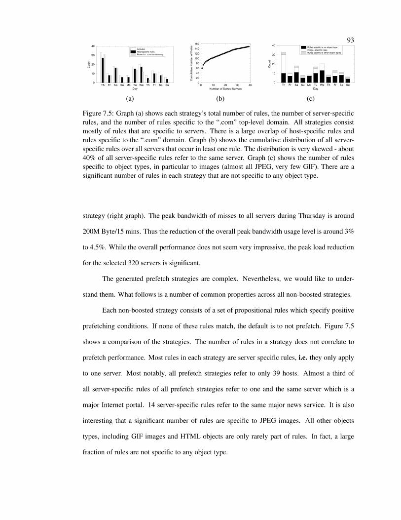
93
Th Fr Sa Su Mo Tu We Th Fr Sa SuDay
0
10
20
30
40
Coun
t
All rulesHost specific rulesRules for .com domain only
0 10 20 30 40Number of Sorted Servers
020406080
100120140160
Cum
ulat
ive N
umbe
r of R
ules
Th Fr Sa Su Mo Tu We Th Fr Sa SuDay
0
10
20
30
40
Coun
t
Rules specific to no object typeImage−specific rulesRules specific to other object types
(a) (b) (c)
Figure 7.5: Graph (a) shows each strategy’s total number of rules, the number of server-specificrules, and the number of rules specific to the “.com” top-level domain. All strategies consistmostly of rules that are specific to servers. There is a large overlap of host-specific rules andrules specific to the “.com” domain. Graph (b) shows the cumulative distribution of all server-specific rules over all servers that occur in least one rule. The distribution is very skewed - about40% of all server-specific rules refer to the same server. Graph (c) shows the number of rulesspecific to object types, in particular to images (almost all JPEG, very few GIF). There are asignificant number of rules in each strategy that are not specific to any object type.
strategy (right graph). The peak bandwidth of misses to all servers during Thursday is around
200M Byte/15 mins. Thus the reduction of the overall peak bandwidth usage level is around 3%
to 4.5%. While the overall performance does not seem very impressive, the peak load reduction
for the selected 320 servers is significant.
The generated prefetch strategies are complex. Nevertheless, we would like to under-
stand them. What follows is a number of common properties across all non-boosted strategies.
Each non-boosted strategy consists of a set of propositional rules which specify positive
prefetching conditions. If none of these rules match, the default is to not prefetch. Figure 7.5
shows a comparison of the strategies. The number of rules in a strategy does not correlate to
prefetch performance. Most rules in each strategy are server specific rules, i.e. they only apply
to one server. Most notably, all prefetch strategies refer to only 39 hosts. Almost a third of
all server-specific rules of all prefetch strategies refer to one and the same server which is a
major Internet portal. 14 server-specific rules refer to the same major news service. It is also
interesting that a significant number of rules are specific to JPEG images. All other objects
types, including GIF images and HTML objects are only rarely part of rules. In fact, a large
fraction of rules are not specific to any object type.

94
7.8 Discussion
The results show (a) and that there is considerable “prefetchable” data available for band-
width smoothing and (b) that automated machine learning is a promising method to rapidly and
automatically develop prefetch strategies.
Our results assume a loss ratio of one. The loss ratio is defined as the cost of false
positives over the cost of false negatives. A loss ratio > 1.0 means that accuracy is valued
higher than coverage, and a loss ratio < 1.0 means that coverage is valued higher than accuracy.
The generated prefetch strategies tend to have high accuracy and low coverage. Furthermore,
figure 7.4 shows that our current prefetch strategies do not fully utilize the extra bandwidth
available during off-peak peak periods. We are currently investigating results with smaller loss
ratios to increase coverage at the expense of accuracy.
The training of these strategies, require information obtained directly from Web sites.
Web site scanning consumes considerable bandwidth since at least the entire HTML content
has to be down-loaded plus header information of images and other objects. Clearly, this time
and resource consuming process would make our approach infeasible. However, a well-known
query interface that allows clients to issue a query to a server or a search engine for information
about objects that match certain properties would significantly reduce the overhead (see for
example [16]). There are also a number of promising projects in the Web metadata community
[92] which are interested in a compact representation of Web content. Finally, we expect that
future search engines will provide detailed profiles of Web server content.
7.9 Summary
We defined prefetch performance in terms of bandwidth smoothing and showed how
prefetch performance impacts our analytical model for smoothing potential introduced in Chap-
ter 6. We showed that machine learning is a promising method to automatically generate
prefetch strategies. These strategies were able to prefetch up to 40% of the prefetchable band-

95
width and do so without wasting significant bandwidth.
Chapter 8
Conclusions
8.1 Summary
In this thesis we studied Web proxy server resource utilization under real work loads.
Real workloads enabled us to identify a number of important performance issues which were not
visible in other, benchmark-oriented studies. In particularly we found that latencies introduced
by disk and network I/O have a significant impact on resource utilization. One can replace
a Web proxy server’s network I/O with disk I/O by introducing Web caching. However, to
improve the resource utilization of Web proxy servers one has to increase the Web cache hit
rate and reduce the disk I/O.
We studied two approaches to improve resource utilization. Both approaches take advan-
tage of the fact that enterprise-level Web proxy servers typically have a diurnal traffic pattern
with very predictable peak and off-peak periods. The first approach investigated the reduction
of disk I/O by carefully designing the way a cache architecture utilizes operating system ser-
vices such as the file system buffer cache and the virtual memory system. The second approach
investigated increasing the Web cache hit rate during peak periods by prefetching bandwidth
during off-peak periods.
8.1.1 Resource Utilization
The details of Web traffic have a significant impact on Web proxy server performance.
We studied the performance of two Web proxy server with significantly different architectures
97
(CERN and SQUID) under real workloads. SQUID’s sophisticated architecture should signifi-
cantly improve performance under high load. However, our results do not confirm this and some
of SQUID’s features are often costly to implement. For instance, SQUID uses the CPU cycles it
saved by not forking processes to implement memory management and non-blocking network
communication. CERN’s architecture is inherently inefficient, but manages to efficiently use
underlying operating systems constructs. As a result CERN has comparable performance.
Although hit rate is typically seen as an important factor for network latency and band-
width savings our results show it has a much more profound effect on reducing the resource
utilization. A low hit rate exposes a Web proxy server to more WAN latencies and increases
the number of open connections. This in turn creates more memory pressure and CPU uti-
lization. In extreme cases, CPU utilization can reach 100% in which case the number of open
connections increase even more.
Although SQUID has many features designed to reduce disk traffic, our measurements
did not show any discernable difference between the two architectures. As we have seen in
Chapter 4 the CERN access patterns maps very well to the file system caching strategy, and the
operating system effectively eliminates many of the potential CERN disk accesses.
Another important aspect of this study is the large, diurnal variation of workload. Other
studies such as [107] and [55] confirm that this workload variation is characteristic for enterprise-
level Web proxy servers. To our knowledge, no available Web proxy server is able to take
advantage of unused resources during off-peak periods in order to reduce resource utilization
during peak periods. In Chapter 5 and Chapter 6 we introduced techniques that take advantage
of extra resources availabe during off-peak time.
8.1.2 Reducing Disk I/O
We showed that adjustments to the SQUID architecture can result in a significant reduc-
tion of disk I/O. Web workloads exhibit much of the same reference characteristics as file system
workloads. As with any high performance application it is important to map file system access
98
patterns so that they mimic traditional workloads to exploit existing operating caching features.
Merely maintaining the first level directory reference hierachy and locality when mapping Web
objects to the file system improved the metadata caching and reduced the number of disk I/O’s
by 50%.
The size and reuse patterns for Web objects are also similar. The most popular pages are
small. Caching small objects in memory mapped files allows most of the hits to be captured with
no disk I/O at all. Using the combination of locality-preserving file paths and memory-mapped
files our simulations resulted in disk I/O savings of over 70%.
We explored the interactions of Web cache management strategies with memory-mapped
files. By carefully considering the system level implementation of memory-mapping files, we
were able to design a replacement strategy which significantly reduces disk I/O while maintain-
ing hit rates comparable to LRU. The developed strategy generates information that can be used
for cache compaction, which reduces disk I/O even further.
8.1.3 Increasing Web Cache Hit Rate During Peak Periods
We showed that using extra network resources to prefetch Web content during off-peak
periods can significantly reduce peak bandwidth usage and that these effects are additive to
effects of traditional demand-based caching. A surprising result is that 99% of the prefetchable
bandwidth consists of new objects from known servers. This result is influenced by the fact that
our notion of prefetchability refers to very stable Web content. However, the result indicates
that prefetch approaches which rely solely on access history information might severely limit
their potential coverage of prefetchable bandwidth. We also presented a mathematical model on
how to calculate the benefit of bandwidth-smoothing for a particular bandwidth usage profile.
We defined prefetch performance in terms of bandwidth smoothing and showed how
prefetch performance impacts our analytical model for smoothing potential introduced in Chap-
ter 6. We showed that machine learning is a promising method to automatically generate
prefetch strategies. These strategies were able to prefetch up to 40% of the prefetchable band-
99
width and do so without wasting significant bandwidth.
8.2 Future Work
Internet information server technology is now a fundamental part of computer science
because of the dominant role of the World-Wide Web in today’s computer usage. For this reason
Web services should join the ranks of fundamental computer services, such as file systems. It
is important to not treat world-wide Web services such as a Web proxy server as just another
application but as a service that should be either integrated into an operating system or at least
well accomodated by operating system services.
In this work we have investigated approaches which do not require any modifications
of operating systems. However, our work on reducing disk I/O suggests that some additional
application level control of the buffer cache would be very useful. We are currently investigating
ways to extend the file system interface to facilitate the implementation of application-level
caches.
Our work on bandwidth smoothing study showed the feasibility of a prefetching ap-
proach under assumption of content summary service. The study shows that Web proxy server
access history alone is a poor basis for prefetching but that access history in combination with
a content summary service is a very promising basis for prefetching. We believe that search
engines are today in a good position to offer valuable Web server content summary services that
would greatly facilitate prefetching. Since our prefetching approach is only concerned with very
stable Web content, it is not critical for us that the content summaries are very current. Ideally
however, Web servers would provide a well known query interface for content summaries. We
are currently in the process of designing such an interface.
Bibliography
[1] Marc Abrams, Charles R. Standridge, Ghaleb Abdulla, Step hen Williaams, and Ed-ward A. Fox. Caching proxies: Limitations and potentials. Available on the World-WideWeb at http://ei.cs.vt.edu/˜succeed/WWW4/WWW4.html.
[2] Arnold O. Allen. Probability, Statistics, and Queueing Theory: with ComputerApplications (2nd edition). Academic Press, San Diego, CA, 1990.
[3] Jussara Almeida, Virgilio Almeida, and David Yates. Measuring the Behavior of a World-Wide Web Server. Technical Report CS 96-025, Boston University, October 29 1996.
[4] Jussara Almeida and Pei Cao. Measuring Proxy Performance with the Wisconsin ProxyBenchmark. Technical Report 1373, Computer Science Department, University ofWisconsin-Madison, April 13 1998.
[5] Virgilio Almeida, Azer Bestavros, Mark Crovella, , and Adriana de Oliveira. Character-izing Reference Locality in the WWW. In IEEE PDIS’96: The International Conferencein Parallel and Distributed Information Systems, Miami Beach, Florida, December 1996.IEEE.
[6] Martin F. Arlitt and Carey L. Williamson. Web Server Workload Characterization: TheSearch for Invariants. In ACM Sigmetrics ’96, pages 126–137, Philadelphia, PA, May23-26 1996. ACM Sigmetrics, ACM.
[7] Martin F. Arlitt and Carey L. Williamson. Trace-Driven Simulation of DocumentCaching Strategies for Internet Web Servers. Simulation, 68(1), January 1997.
[8] Anselm Baird-Smith. Jigsaw Overview. Available on the World-Wide Web athttp://www.w3.org/pub/WWW/Jigsaw/, February 24 1997.
[9] Mary G. Baker, John H. Hartman, Michael D. Kupfer, Ken W. Shirriff, and John K.Ousterhout. Measurements of a Distributed File System. In Proceedings fo theSymposium on Operating Systems Principles (SOSP), pages 198–212. ACM, October1991.
[10] Lance Berc, Sanjay Ghemawat, Monika Henzinger, Shun-Tak Leung, Mitch Licht-enberg, Dick Sites, Mark Vandevoorde, Carl Waldspurger, and Bill Weihl. DIG-ITAL Continuous Profiling Infrastructure. Available on the World-Wide Web athttp://www.research.digital.com/SRC/dcpi/papers/osdi96-wip.html, October 1996.
101
[11] Tim Berners-Lee. Hypertext Transfer Protocol (HTTP), working draft. Available onthe World-Wide Web at http://www.w3.org/pub/WWW/Protocols/HTTP/HTTP2.html,November 1993.
[12] Tim Berners-Lee and Dan Connolly. Hypertext Markup Language - 2.0. Available onthe World-Wide Web at http://ds.internic.net/rfc/rfc1866.txt, November 1995.
[13] Tim Berners-Lee, R. Fielding, and H. Frystyk. Hypertext Transfer Protocol – HTTP/1.0.Available on the World-Wide Web at http://ds.internic.net/rfc/rfc1945.txt, May 1996.
[14] A. Bestavros and C. Cunha. Server-initiated Document Dissemination for the WWW.IEEE Data Engineering Bulletin, 19:3–11, September 1996.
[15] Azer Bestavros. Speculative Data Dissemination and Service to Reduce Server Load,Network Traffic and Service Time for Distributed Information Systems. In ICDE’96:The 1996 International Conference on Data Engineering, New Orleans, Louisiana, March1996.
[16] Krishna Bharat, Andrei Broder, Monika Henzinger, Puneet Kumar, and Suresh Venkata-subramanian. The connectivity server: fast access to linkage information on the web.Computer Networks and ISDN Systems, 30(1-7), April 1998. Special Issue on SeventhInternational World-Wide Web Conference, April 14-18, 1998, Brisbane, Australia.
[17] N. Borenstein and N. Freed. MIME (Multipurpose Internet Mail Extensions) Part One:Meachanisms for Specifying and Describing the Format of Internet Message Bodies.Available on the World-Wide Web at http://ds.internic.net/rfc/rfc1521.txt, September1993.
[18] C. Mic Bowman, Peter B. Danzig, Darren R. Hardy, Udi Man ber, Michael F. Schwartz,and Duane P. Wessels. Harvest: A scalable, customizable discovery and access system.Technical Report CU-CS-732-94, Department of Computer Science, University of Col-orado, Boulder , CO, August 1994 (revised March 1995) 1994.
[19] Lee Breslau, Pei Cao, Li Fan, Graham Phillips, and Scott Shenker. Web Caching andZipf-like Distributions: Evidence and Implications. Technical Report 1371, ComputerSciences Dept, Univ. of Wisconsin-Madison, April 1998.
[20] Inc. CacheFlow. Active Web Caching Technology. Available on the World Wide Web athttp://www.cacheflow.com/info/docs/wp/activecaching.html, February 24 1999.
[21] Brad Calder, Dirk Grunwald, Michael Jones, Donald Lindsay, James Martin, MichaelMozer, and Benjamin Zorn. Evidence-based static branch prediction using machinelearning. ACM Transactions on Programming Languages and Systems, 19(1):188–223,January 1997.
[22] Pei Cao. Characterization of Web Proxy Traffic and Wisconsin Proxy Benchmark 2.0. InW3C Web Characterization Workshop, Nov 5 1998.
[23] Pei Cao and Sandy Irani. Cost-Aware Web Proxy Caching. In Usenix Symposium onInternet Technologies and Systems (USITS), pages 193–206, Monterey, CA, USA, De-cember 8-11 1997. Usenix.
102
[24] Anawat Chankhunthod, Peter B. Danzig, Chuck Neerdaels, Michael F. Schwartz, andKurt J. Worrell. A Hierarchical Internet Object Cache. In 1996 USENIX TechnicalConference, San Diego, CA, January 1996. USENIX.
[25] D. Brent Chapman and Elizabeth D. Zwicky. Building Internet Firewalls. O’Reilly, Se-bastopol, CA, 1995.
[26] Inc. Cobalt Networks. Cobalt Caching Solutions. Available on the World Wide Web athttp://www.cobaltmicro.com/products/cache/page cache.html, August 5 1998.
[27] Edith Cohen, Balachander Krishnamurthy, and Jennifer Rexford. Improving End-to-EndPerformance of the Web Using Server Volumes and Proxy Filters. In SIGCOMM’98,Vancouver, BC, September 1998. ACM.
[28] William W. Cohen. Fast Effective Rule Induction. In Machine Learning: Proceedings ofthe Twelfth International Conference (ML95), 1995.
[29] William W. Cohen. The RIPPER Rule Learner. Available on the World-Wide Web athttp://www.research.att.com/˜wcohen/ripperd.html, November 25 1996.
[30] Dan Connolly and Tim Berners-Lee. Names and Addresses, URIs, URLs, URNs, URCs.Available on the World-Wide Web at http://www.w3.org/pub/WWW/Addressing/, De-cember 1990.
[31] Netscape Communications Corporation. NetscapeProxy Server. Available on the World-Wide Web athttp://home.netscape.com/comprod/server central/product/proxy/index.html, 1997.
[32] Mark Crovella and Paul Barford. The Network Effects of Prefetching. Technical Report97-002, Boston University, CS Dept., February 7 1997.
[33] Mark Crovella and Paul Barford. The Network Effects of Prefetching. In IEEEINFOCOM’98, San Francisco, CA, 29 March - 2 April 1998. IEEE.
[34] Carlos R. Cunha, Azer Bestavros, and Mark E. Crovella. Characteristics of WWWClient-based Traces. Technical Report BU-CS-95-010, Computer Science Department,Boston University, July 18 1995.
[35] Kenneth M. Curewitz, P. Krishnan, and Jeffrey Scott Vitter. Practical prefetching viaData Compression. In SIGMOD’93, pages 257–266. ACM, May 1993.
[36] Peter Danzig. NetCache Architecture and Deployment. Available on the World WideWeb at http://www.netapp.com/technology/level3/3029.html, January 14 1999.
[37] Arjan de Vet. Squid new disk storage scheme. Available on the World Wide Web athttp://www.iaehv.nl/users/devet/squid/new store/, November 17 1997.
[38] Thomas G. Dietterich. Machine Learning. ACM Computing Surveys,28(4es), December 1996. Available on the World-Wide Web athttp://www.acm.org/pubs/citations/journals/surveys/1996-28-4es/a3-dietterich/.
[39] Thomas G. Dietterich. Machine-Learning Research: Four Current Directions. AIMagazine, 18(4):97–136, Winter 1997.
103
[40] Adam Dingle and Tomas Partl. Web Cache Coherence. In Fifth International World-WideWeb Conference, Paris, France, May 6-10 1996. W3C.
[41] Fred Douglis, Anja Feldmann, Balachander Krishnamurthy, and Jeffrey Mogul. Rate ofChange and other Metrics: a Live Study of the World-Wide Web. In Usenix Symposiumon Internet Technologies and Systems (USITS), Monterey, CA, USA, December 8-111997. Usenix.
[42] Brad Duska, David Marwood, and Michael J. Feeley. The Measured Access Charac-teristics of World-Wide Web Client Proxy Caches. In Usenix Symposium on InternetTechnologies and Systems (USITS), Monterey, CA, USA, December 8-11 1997. Usenix.
[43] W. Effelsberg and T. Haerder. Principles of Database Buffer Management. ACMTransactions on Database Systems, 9(4):560–595, December 1984.
[44] C. J. G. Evertsz and B. B. Mandelbrot. Multifractal Measures. In H.-O. Petgen, H. Ju-rgens, and D. Saupe, editors, Chaos and Fractals: New Frontiers in Science. SpringerVerlag, New York, 1992.
[45] Li Fan, Quinn Jacobson, and Pei Cao. Potential and Limits of Web Prefetching BetweenLow-Bandwidth Clients and Proxies. In to appear in SIGMETRICS’99, 1999.
[46] Anja Feldmann, Ramn Cceres, Fred Douglis, Gideon Glass, and Michael Rabinovich.Performance of Web Proxy Caching in Heterogeneous Bandwidth Environments. InINFOCOM’99. IEEE, 1999.
[47] Anja Feldmann, Anna Gilbert, and Walter Willinger. Data networks as cascades: Ex-plaining the multifractal nature of Internet WAN traffic. In SIGCOMM’98, Vancouver,BC, September 1998. ACM.
[48] R. Fielding, J. Gettys, J. C. Mogul, H. Frystyk, and T. Berners-Lee. Hy-pertext Transfer Protocol – HTTP/1.1. Available on the World-Wide Web athttp://www.w3.org/pub/WWW/Protocols/rfc2068/rfc2068, January 1997.
[49] D. H. Fisher, M. J. Pazzani, and P. Langley.Concept Formation: Knowledge and Experience in Unsupervised Learning. MorganKaufmann, San Mateo, CA, 1991.
[50] Stewart Forster. Personal Communication. Description of disk I/O in Squid 1.2, August14 1998.
[51] Y. Freund and R. E. Schapire. A Decision-Theoretic Generalization of On-Line Learningand an Application to Boosting. In Proceedings of the Second European Conference onComputational Learning Theory, pages 23–37, Berlin, 1995. Springer Verlag.
[52] Y. Freund and R. E. Schapire. Experiments with a New Boosting Algorithm. In L. Saitta,editor, Proceedings of the Thirteenth International Conference on Machine Learning,pages 148–156, San Francisco, CA, 1996. Morgan Kaufmann.
[53] Steven Glassman. A caching relay for the world-wide web. In First InternationalWorld-Wide Web Conference, pages 69–76. W3O, May 1994.
104
[54] Richard Golding, Peter Bosch, and John Wilkes. Idleness is not Sloth. Technical ReportHPL-96-140, HP Labs, Hewlett-Packard, October 4 1996.
[55] Steven D. Gribble and Eric A. Brewer. System design issues for Internet MiddlewareServices: Deductions from a large client trace. In Usenix Symposium on InternetTechnologies and Systems (USITS), Monterey, CA, USA, December 8-11 1997. Usenix.
[56] Jim Griffioen and Randy Appleton. Reducing File System Latency Using a Predic-tive Approach. In USENIX Summer 1994 Technical Conference, 197-208, June 1994.Usenix.
[57] James Gwertzman and Marga Seltzer. The Case for Geographical Push Caching. InFifth Annual Workshop on Hot Operating Systems, pages 51–55, Orcas Island, WA,May 1995.
[58] James Gwertzman and Marga Seltzer. World-Wide Web Cache Consistency. In 1996USENIX Technical Conference, San Diego, CA, Jan 1996. USENIX.
[59] John Heidemann, Katia Obraczka, and Joe Touch. Modeling the Performance of HTTPOver Several Transport Protocols. Submitted to IEEE/ACM Transactions on Networking,November 1996.
[60] John L. Hennessy and David A. Patterson. Computer Architecture: A QuantitativeApproach (2nd edition). Morgan Kaufmann, San Francisco, CA, 1996.
[61] R. Holley and E. C. Waymire. Multifractal Dimensions and Scaling Exponents forStrongly Bounded Random Cascades. Annals of Applied Probability, 2:819–845, 1992.
[62] Ken ichi Chinen and Suguru Yamaguchi. An Interactive Prefetching Proxy Server forImprovement of WWW Latency. In inet 97, Kuala Lumpur, Malaysia, June 24-27 1997.ISOC.
[63] Inktomi. Inktomi Traffic Server – Product Info. Available on the World Wide Web athttp://www.inktomi.com/products/traffic/product.html, February 4 1999.
[64] Raj Jain. The Art of Computer Systems Performance Analysis. Wiley, New York, 1991.
[65] Jaeyeon Jung. Proxy Benchmarks. Available on the World Wide Web athttp://www.ircache.net/Hit-N-Miss/archive/n002.19980625/benchmarks.tbl.html, June 91998.
[66] L. Kleinrock. Queueing Systems, Volume 1: Theory. John Wiley & Sons, 1975.
[67] L. Kleinrock. Queueing Systems, Volume 2: Computer Applications. John Wiley &Sons, 1976.
[68] Balachander Krishnamurthy and Craig E. Wills. Study of Piggyback Cache Validation forProxy Caches in the World-Wide Web. In Usenix Symposium on Internet Technologiesand Systems (USITS), Monterey, CA, USA, December 8-11 1997. Usenix.
[69] Thomas Kroeger, Jeffrey Mogul, and Carlos Maltzahn. Digi-tal’s Web Proxy Traces. Available on the World-Wide Web atftp://ftp.digital.com/pub/DEC/traces/proxy/webtraces.html, October 1996.
105
[70] Thomas M. Kroeger, Darrel D. E. Long, and Jeffrey C. Mogul. Exploring the Boundsof Web Latency Reduction from Caching and Prefetching. In Usenix Symposium onInternet Technologies and Systems (USITS), Monterey, CA, USA, December 8-11 1997.Usenix.
[71] Edward D. Lazowska, John Zahorjan, G. Scott Graham, and Kenneth C. Sevcik.Quantitative System Performance: Computer System Analysis Using Queueing NetworkModels. Prentice-Hall, Inc., Englewood Cliffs, NJ, 1984.
[72] Kevin Littlejohn. communications on [email protected]. First prototype of squidfs,January 29 1999.
[73] Tong Sau Loon and Vaduvur Bharghavan. Alleviating the Latency and Bandwidth Prob-lems in WWW Browsing. In Usenix Symposium on Internet Technologies and Systems(USITS), Monterey, CA, USA, December 8-11 1997. Usenix.
[74] Paolo Lorenzetti, Luigi Rizzo, and Lorenzo Vicisano. Replacement Policies for a ProxyCache. Available on the World-Wide Web at http://www.iet.unipi.it/˜luigi/caching.ps.gz,August 2 1996.
[75] Ari Luotonen. Web Proxy Servers. Prentic Hall, Upper Saddle River, NJ, 1998.
[76] Ari Luotonen, Henrik Frystyk Nielsen, and Tim Berners-Lee. CERN httpd 3.0A. Avail-able on the World-Wide Web at http://www.w3.org/pub/WWW/Daemon/, July 15 1996.
[77] Carlos Maltzahn, Kathy Richardson, and Dirk Grunwald. Performance Issues of Enter-prise Level Proxies. In SIGMETRICS ’97, pages 13–23, Seattle, WA, June 15-18 1997.ACM.
[78] Carlos Maltzahn, Kathy Richardson, and Dirk Grunwald. Reducing the Disk I/O of WebProxy Server Caches. In Usenix Annual Technial Conference, Monterey, CA, June 6-111999.
[79] Carlos Maltzahn, Kathy Richardson, Dirk Grunwald, and James Martin. On BandwidthSmoothing. In 4th International Web Caching Workshop (WCW’99), San Diego, CA,March 30 - April 2 1999.
[80] Evangelos P. Markatos and Catherine E. Chronaki. A Top 10 Approach for Prefetchingthe Web. In INET’98, Geneva, July 21-24 1998. Internet Society.
[81] Marshall K. McKusick, William N. Joy, Samual J. Leffler, and Robert S. Fabry. A FastFile System for UNIX. ACM Transactions on Computer Systems, 2(3):181–197, August1984.
[82] Marshall Kirk McKusick, Keith Bostic, Michael J. Karels, and John S. Quarter-man. The Design and Implementation of the 4.4BSD Operating System. Addison Wes-ley, Reading, Massachusetts, 1996.
[83] Ingrid Melve, Lars Slettjord, Henny Bekker, and Ton Verschuren. Building a WebCaching System - Architectural Considerations. In NLANR Web Cache Workshop,Boulder, CO, June 9 - 10 1997.
106
[84] P. Mockapetris. Domain Names - Concepts and Facilities. Available on the World-WideWeb at ftp://ftp.internic.net/rfc/rfc1034.txt, November 1987.
[85] P. Mockapetris. Domain Names - Implementation and Specification. Available on theWorld-Wide Web at ftp://ftp.internic.net/rfc/rfc1035.txt, November 1987.
[86] Jeff Mogul. Personal communication. Idea to mmap a large file for objects less or equalthan system page size, August 1996.
[87] Jeffrey Mogul and Paul J. Leach. Simple Hit Metering and Usage-Limiting for HTTP.Available on the World-Wide Web at http://ds.internic.net/internet-drafts/draft-ietf-http-hit-metering-02.txt, March 1997.
[88] Jeffrey C. Mogul, Fred Douglis, Anja Feldman, and Balachander Krishnamurthy. Po-tential benefits of delta-encoding and data compression for HTTP. In SIGCOMM ’97,Cannes, France, September 1997. ACM.
[89] Norifumi Nishikawaa, Takafumi Hosokawaa, Yasuhide Morib, Kenichi Yoshidab, andHiroshi Tsuji. Memory-based architecture for distributed WWW caching proxy.Computer Networks and ISDN Systems, 30(1-7), April 1998. Special Issue on SeventhInternational World-Wide Web Conference, April 14-18, 1998, Brisbane, Australia.
[90] Mark Nottingham. Optimizing Object Freshness Controls in Web Caches. In 4thInternational Web Caching Workshop (WCW’99), San Diego, CA, March 31 - April2 1999.
[91] Thomas P. Novak and Donna L. Hoffman. New Metrics for New Media: To-ward the Development of Web Measurement Standards. Available on the World-Wide Web at http://www2000.ogsm.vanderbilt.edu/novak/web.standards/webstand.html,September 26 1996.
[92] International Federation of Library Associations and Institutions (IFLA). Digital Li-braries: Metadata resources page. Available on the World Wide Web at http://www.nlc-bnc.ca/ifla/II/metadata.htm, August 31 1998.
[93] John Ousterhout, Herve Da Costa, David Harrison, John A. Kunze, Mike Kupfer, andJames G. Thompson. A Trace-Driven Analysis of the UNIX 4.2 BSD File System. Tech-nical Report UCB/CSD 85/230, University of California, Berkeley, April 1985.
[94] Venkata N. Padmanabhan and Jeffrey C. Mogul. Improving HTTP Latency. InProceedings of Second WWW Conference ’94: Mosaic and the Web, pages 995–1005,Chicago, IL, October 17-19 1994.
[95] Venkata N. Padmanabhan and Jeffrey C. Mogul. Using Predictive Prefetching to ImproveWorld-Wide Web Latency. In SIGCOMM’96, pages 22–36. ACM, July 1996.
[96] Vivek S. Pai, Mohit Aron, Gaurav Banga, Michael Svendsen, Peter Druschel, WillyZwaenepoel, and Erich Nahum. Locality-Aware Request Distribution in Cluster-basedNetwork Servers. In Eighth International Conference on Architectural Support forProgramming Languages and Operating Systems (ASPLOS-VIII), San Jose, CA, Oc-tober 4-7 1998.
107
[97] Mark Palmer and Stanley B. Zdonik. Fido: A Cache that Learns to Fetch. In 17thInternational Conference on Very Large Database (VLDB’91), pages 255–264, Septem-ber 1991.
[98] Vern Paxson. Why We Don’t Know How To Simulate The Internet. In Proceedings ofthe 1997 Winter Simulation Conference, December 1997.
[99] Vern Paxson and Sally Floyd. Wide-Area Traffic: The Failure of Poisson Modeling.IEEE/ACM Transactions on Networking, 3(3):226–244, June 1995.
[100] James Pitkow. In Search of Reliable Usage Data on the WWW. In WWW 6, 1997.
[101] Jon B. Postel. Transmission Control Protocol, RFC 793,. Available on the World-WideWeb at, September 1981.
[102] J. Ross Quinlan. C4.5: Programs for machine learning. Morgan Kaufmann, San Mateo,CA, 1993.
[103] Kathy J. Richardson. I/O Characterization and Attribute Caches for Improved I/O SystemPerformance. Technical Report CSL-TR-94-655, Stanford University, Dec 1994.
[104] Luigi Rizzo and Lorenzo Vicisano. Replacement Policies for a Proxy Cache. TechnicalReport RN/98/13, University College London, Department of Computer Science, 1998.
[105] John T. Robinson and Murthy V. Devarakonda. Data Cache Management UsingFrequency-Based Replacement. In SIGMETRICS’90, pages 134–142, Boulder, CO,May 22-25 1990. ACM.
[106] J. A. Rolia and K. C. Sevcik. The Method of Layers. IEEE Transactions on SoftwareEngineering, 21(8):689–699, August 1995.
[107] Alex Rousskov. On Performance of Caching Proxies. Available on the World-WideWeb at http://www.cs.ndsu.nodak.edu/˜rousskov/research/cache/squid/profiling/papers/sigmetrics.html, 1997.
[108] Alex Rousskov. Web Polygraph. Available on the World Wide Web athttp://www.ircache.net/Polygraph/, February 2 1999.
[109] Alex Rousskov and Valery Soloviev. A Performance Study of the Squid Proxy onHTTP/1.0. to appear in World-Wide Web Journal , Special Edition on WWW Charac-terization and Performance Evaluation, 1999.
[110] Alex Rousskov, Valery Soloview, and Igor Tatarinov.Static Caching. Available on the World-Wide Web athttp://www.nlanr.net/Cache/Workshop97/Papers/Rousskov/rousskov.html, June 1997.
[111] Peter Scheuermann, Junho Shim, and Radek Vingralek. A Case for Delay-ConsciousCaching of Web Documents. In Sixth International World-Wide Web Conference, SantaClara, CA, April 7-11 1997.
[112] Inc SkyCache. Renovating the Internet. Available on the World Wide Web athttp://www.skycache.com/whitepaper.html, Feb 5 1998.
108
[113] Standard Performance Evaluation Corp. (SPEC). SPECweb96 Benchmark. Available onthe World-Wide Web at http://www.specbench.org/osg/web96/, July 1996.
[114] Simone E. Spero. Analysis of HTTP Performance Problems. Available on the World-Wide Web at http://sunsite.unc.edu/mdma-release/http-prob.html, June 2 1995.
[115] Carl D. Tait and Dan Duchamp. Detection and Exploitation of File Working Sets. Tech-nical Report CUCS-050-90, Computer Science Department, Columbia University, 1990.
[116] Squid Users. Squid-users mailing list archive. Available on the World-Wide Web athttp://squid.nlanr.net/Mail-Archive/squid-users/hypermail.html, August 1998.
[117] Jeffrey Scott Vitter and P. Krishnan. Optimal Prefetching via Data Compression. Journalof the ACM, 143(5):121–130, September 1996.
[118] Stuart Wachsberg, Thomas Kunz, and Johnny Wong. Fast World-Wide WebBrowsing Over Low-Bandwidth Links. Available on the World-Wide Web athttp://ccnga.uwaterloo.ca/˜sbwachsb/paper.html, 1996.
[119] Zheng Wang and Jon Crowcroft. Prefetching in World-Wide Web. Available on theWorld-Wide Web at http://www.cs.ucl.ac.uk/staff/zwang/papers/prefetch/Overview.html,January 30 1996.
[120] Bob Warfield, Terry Mueller, and Peter Sember. Monitoring the Performance of a Cachefor Broadband Customers. In INET’98, Geneva, Switzerland, June 22-25 1998.
[121] Duane Wessels. Intelligent caching for world-wide web objects. Available on the World-Wide Web at http://morse.colorado.edu/˜wessels/Proxy/wessels-inet95.A4.ps.gz, 1995.
[122] Duane Wessels. Personal communication. during which became clear that Squid1.0.beta17 has a memory management bug, August 1996.
[123] Duane Wessels. Squid Internet Object Cache. Available on the World-Wide Web athttp://squid.nlanr.net/Squid/, May 1996.
[124] Duane Wessels. Hierarchical Web Caching. Slides of talk at NANOG ’97, Available onthe World-Wide Web at http://www.nlanr.net/˜wessels/Viewgraphs/NANOG-11Feb97/,February 1997.
[125] Duane Wessels. SQUID Frequently Asked Questions. Available on the World-Wide Webat http://squid.nlanr.net/Squid/FAQ.html, January 1997.
[126] Stephen Williams, Marc Abrams, Charles R. Standridge, Ch aleb Abdulla, and Ed-ward A. Fox. Removal policies in network caches for world-wide web documents. InACM SIGCOMM, pages 293–305, Stanford, CA, August 1996.
[127] W. Willinger, V. Paxson, and M. S. Taqqu. Self-similarity and Heavy Tails: Struc-tural Modeling of Network Traffic. In R. Adler, R. Feldman, and M. S. Taqqu, editors,A Practical Guide to Heavy Tails: Statistical Techniques for Analyzing Heavy-TailedDistributions. Birkhauser, Boston, MA, USA, 1998.
109
[128] C. Murray Woodside, John E. Neilson, Dorina C. Petriu, and Shikharesh Majumdar. TheStochastic Rendezvous Network Model for Performance of Synchronous Client-Server-like Distributed Software. IEEE Transactions on Computers, 44(1):20–34, January 1995.
[129] Roland P. Wooster and Marc Abrams. Proxy Caching That Estimates Page Load Delays.In Sixth International World-Wide Web Conference, Santa Clara, CA, April 7-11 1997.
[130] George Kingsley Zipf. Relative Frequency as a Determinant of Phonetic Change.reprinted from Harvard Studies in Classical Philiology, XL, 1929.