Improving Gas Well Cementing Through Cement Pulsation

GTI Contract Number 6011

Project Technical Report

CTES, L.C. 9870 Pozo Ln, Conroe, TX 77303

Phone 936-521-2209 Fax: 936-521-2297 e-mail: ken.newman@ctes.com

www.ctes.com

LEGAL NOTICE This report was prepared by CTES, L.C. as an account of work sponsored by Gas Research Institute (GRI). Neither GRI, members of GRI, nor any person acting on behalf of either: a. MAKES ANY WARRANTY OR REPRESENTATION, EXPRESS OR IMPLIED WITH RESPET TO THE ACCURACY, COMPLETENESS, OR USEFULNESS OF THE INFORMATION CONTAINED IN THIS REPORT, OR THAT THE USE OF ANY INFORMATION, APPARATUS, METHOD, OR PROCESS DISCLOSED IN THIS REPORT MAY NOT INFRINGE PRIVATELY OWNED RIGHTS, OR b. ASSUMES ANY LIABILITY WITH RESPECT TO THE USE OF, OR FOR ANY AND ALL DAMAGES RESULTING FROM THE USE OF, ANY INFORMATION, APPARATUS, METHOD, OR PROCESS DISCLOSED IN THIS REPORT. c. REFERENCE TO TRADE NAMES OR SPECIFIC COMMERCIAL PRODUCTS, COMMODITIES, OR SERVICES IN THIS REPORT DOES NOT REPRESENT OR CONSTITUTE AN ENDORCEMENT, RECOMMENDATION, OR FAVORING BY GRI OR ITS CONTRACTORS OF THE SPECIFIC COMMERCIAL PRODUCT, COMMODITY, OR SERVICE.

REPORT DOCUMENTATION PAGE Form Approved

OMB No. 0704-0188

Public reporting burden for this collection of information is estimated to average 1 hour per response, including the time for reviewing instructions, searching existing data sources, gathering and maintaining the data needed, and completing and reviewing the collection of information. Send comments regarding this burden estimate or any other aspect of this collection of information including suggestions for reducing this burden to Washington Headquarters Services, Directorate for Information Operations and Reports, 1215 Jefferson Davis Highway, Suite 1204, Arlington, VA 22202-4302, and to the Office of Management and Budget, Paperwork Reduction Project (0704-0188), Washington, D.C. 20503.

1. AGENCY USE ONLY (Leave blank) 2. REPORT DATE

September 2001 3. REPORT TYPE AND DATES COVERED

4. TITLE AND SUBTITLE

Improving Gas Well Cementing Through Cement Pulsation

5. FUNDING NUMBERS

GRI contract no. 6011

6. AUTHOR(S)

K. Newman, P.E., - CTES, L.C. Dr. Andrzej (Andrew) Wojtanowicz. P.E. - LSU

7. PERFORMING ORGANIZATION NAME(S) AND ADDRESS(ES)

CTES, L.C. 9870 Pozos Lane, Conroe, TX 77303 LSU - 449 Daventry Drive, Baton Rouge, Louisiana 70808

8. PERFORMING ORGANIZATION REPORT NUMBER

9. SPONSORING/MONITORING AGENCY NAME(S) AND ADDRESS(ES)

GTI 1700 S. Mount Prospect Rd. Des Plaines, IL 60018

10. SPONSORING/MONITORING AGENCY REPORT NUMBER

GRI-01/0179.1

11. SUPPLEMENTARY NOTES

12a. DISTRIBUTION/AVAILABILITY STATEMENT

12b. DISTRIBUTION CODE

13. ABSTRACT (Maximum 200 words)

CP is a process in which pressure pulses of about 100 psi are applied to the top of the cement column immediately after the cement is pumped. A research project was performed to determine whether Cement Pulsation (CP) would reduce the influx of fluids into the wellbore once the cement is placed. Such fluid influxes result in problems such a gas migration and shallow water flows which are very costly to the oil and gas industry. The results from this project show that cement pulsation:

Sends pulses through mud and cement columns to significant depths Shears the cement preventing it from forming gel strength, and supporting itself on the walls of the

borehole and casing, thus preventing a reduction in hydrostatic pressure. Significantly reduces the probability of gas migration problems. Provides information about the setting of the cement and the quality of the cement job.

14. SUBJECT TERMS

Cementing, Cement pulsation, gas migration

15. NUMBER OF PAGES

91 16. PRICE CODE

17. SECURITY CLASSIFICATION OF REPORT

Unclassified

18. SECURITY CLASSIFICATION OF THIS PAGE

Unclassified

19. SECURITY CLASSIFICATION OF ABSTRACT

Unclassified

20. LIMITATION OF ABSTRACT

NSN 7540-01-280-5500 Standard Form 298 (Rev.2-89)

Research Summary Title Improving Gas Well Cementing Through Cement Pulsation Conroe, Montgomery County, Texas Contractor(s) CTES, L.C. - GRI Contract Number 6011 Principal Investor(s) CTES, L.C. Report Type Final Report Report Period August, 1999 - September, 2001 Objective The objectives of this project were:

Determine if cement pulsation (CP) prevented the reduction in hydrostatic pressure while the cement was setting

Determine if the pulses would travel to the bottom of an average depth well Model the CP process to better understand the physics Determine if CP does mitigate gas migration Determine if surface measurements made during the CP process could yield information

about the cement setting process Transfer CP technology to the industry

Technical Perspective During the cement setting process the hydrostatic pressure in the cement decreases. Often this decrease in hydrostatic pressure allows formation fluids to migrate into the cement. Gas migration problems occur when gas migrates through the cement to other formations or to the surface. Repairing gas migration problems costs the oil and gas industry an estimated 470 million dollars per year. This project continues work begun several years before by John Haberman, then at Texaco, to determine whether applying pressure pulses of about 100 psi to the top of the fluid column in the casing annulus above the cement, would improve the cement job and mitigate gas migration problems.

Technical Approach There were several aspects to the technical approach:

An instrumented CP system was developed to perform the CP process and acquire various measurements during the process.

CP was performed on several wells to prove the system and better understand the process. A downhole pressure and temperature measuring system was developed to measure the

temperature and pressure in the cement during the CP process. This system was used on two wells.

Mathematical models of the CP process were developed and use to analyze the response of the cement to the pulses.

A series of wells in areas with significant gas migration problems were pulsed to prove that CP does indeed mitigate gas migration.

Results This project showed that:

CP does prevent the reduction of hydrostatic pressure while cement is setting CP does reduce or eliminate gas migration problems The pulses do reach the bottom of wells of average depth Measurement of the compressible volume (CV) during the CP process yields useful

information about the cement setting process. Numerous articles and papers were published to inform the industry about CP and its

results. CP was commercialized in Alberta Canada

Project Implications Once CP is used extensively throughout the oil and gas industry, the industry will obtain significant savings due to reduced gas migration problems. Also, the ability to determine when the cement is set by monitoring the CV will eliminate wasted rig time from “waiting on cement” when the cement is already set. Finally, the industry will obtain a better understanding of cement chemistry and rheology from this process.

MEMORANDUM TO: Gas Research Institute (GRI) FROM: CTES, L.C. SUBJECT: Reports GRI-01/0179.1 and GRI-01/0179.2 GRI is authorized to publish, have published, reproduce, have reproduced, distribute, have distributed, and sell or have sold on its behalf this copyrighted work. Permission for further reproduction must be obtained from the copyright owner. __________________________________ (Signature of copyright owner or authorized representative) __________________________________ CTES, L.C. (Signature of copyright owner or authorized representative) __________September 22, 2001____________ Date

1

Table of Contents

Executive Summary ............................................................................................................ 2 Introduction ......................................................................................................................... 4

CP Process ..................................................................................................................... 5 Task List .......................................................................................................................... 7

Task 1 - Gas Migration and the Problems It Causes ........................................................... 8 Task 2 – Identification of Market Barriers ............................................................................ 9 Task 3 - Determine the Effect of CP on the Cement Sheath ............................................. 12 Task 4 - Development of a Self-Contained CP Unit (CPU) ............................................... 13

CPU Skid ....................................................................................................................... 13 CP Unit Data Acquisition and Control System (DAS) .................................................... 14

Task 5- Monitoring Tools and Procedures ........................................................................ 15 Task 6 – Field Evaluation of CP ........................................................................................ 17

CP Field Evaluations Overview ..................................................................................... 17 CP #01, Woolverton #1 ................................................................................................. 17 CP #02, Yturria #3-7 ...................................................................................................... 19 CP #03, Yturria #4-3 ...................................................................................................... 23 CP #04, Campbell #4 .................................................................................................... 26 CP #05, York #5 ............................................................................................................ 29 CP #06, Dinn #2 ............................................................................................................ 31 CP #08, Phelan #1 ........................................................................................................ 34 CP #09, Lewis #B-2 ....................................................................................................... 37

Task 7 – CP Tests with Downhole Measurements ............................................................ 43 CP #07 Mestena #E-25 ................................................................................................. 43 CP #10, Well KWU4082 ................................................................................................ 48 CP # 11, KWU4057 ...................................................................................................... 56

Task 8 - Determine the effectiveness of CP for preventing gas migration ........................ 61 Task 9 - Methods for CP Analysis, Design, and Control ................................................... 63

TASK OBJECTIVE ........................................................................................................ 63 PHYSICAL ANALYSIS OF THE CP PROCESS ............................................................ 63 COMPRESSIBILITY OF CEMENTED WELL ANNULUS .............................................. 64 ALGORITHM FOR CP PROCESS DESIGN ................................................................. 66

Task 10 – Diagnostic model and analysis method for monitoring pressure pulse transmission and quality of CP treatment ......................................................................... 72 Task 11 – Laboratory Evaluation of Cement Slurry for CP Applications ........................... 84

Task Objective ............................................................................................................... 84 Test Protocol ................................................................................................................. 84 Example Application of Testing Method to Fluids and Comparison to Field Results for KWU 4082 ..................................................................................................................... 86

Task 12 – Transfer of CP technology to Industry .............................................................. 91

2

EXECUTIVE SUMMARY

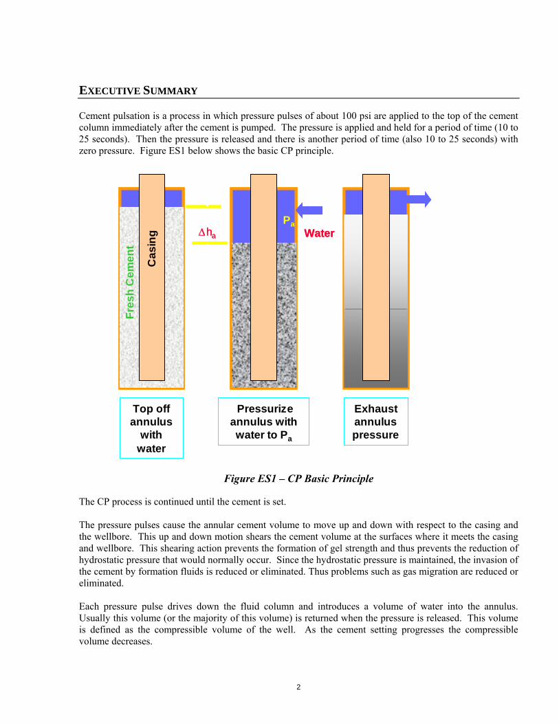
Cement pulsation is a process in which pressure pulses of about 100 psi are applied to the top of the cement column immediately after the cement is pumped. The pressure is applied and held for a period of time (10 to 25 seconds). Then the pressure is released and there is another period of time (also 10 to 25 seconds) with zero pressure. Figure ES1 below shows the basic CP principle.

Figure ES1 – CP Basic Principle

The CP process is continued until the cement is set. The pressure pulses cause the annular cement volume to move up and down with respect to the casing and the wellbore. This up and down motion shears the cement volume at the surfaces where it meets the casing and wellbore. This shearing action prevents the formation of gel strength and thus prevents the reduction of hydrostatic pressure that would normally occur. Since the hydrostatic pressure is maintained, the invasion of the cement by formation fluids is reduced or eliminated. Thus problems such as gas migration are reduced or eliminated. Each pressure pulse drives down the fluid column and introduces a volume of water into the annulus. Usually this volume (or the majority of this volume) is returned when the pressure is released. This volume is defined as the compressible volume of the well. As the cement setting progresses the compressible volume decreases.

Top off annulus

with water

Pressurize annulus with water to Pa

Exhaustannulus pressure

ha

Pa

Ca

sin

g

Fre

sh

Ce

me

nt

Water

Top off annulus

with water

Pressurize annulus with water to Pa

Exhaustannulus pressure

ha

Pa

Ca

sin

g

Fre

sh

Ce

me

nt

Water

3

This research project has proven the following major points about CP:

The pulses do not damage the cement sheath The attenuation of the pressure pulses is small, so that they are capable of reaching the bottom of

fairly deep wells. Measurement of the compressible volume yields information about the setting process of the

cement. CP was used in shallow gas fields in Alberta Canada in which 25% to 50% of the wells have historically had gas migration problems. Of the 22 wells pulsed and completed in these fields to date, none have experienced gas migration problems.

4

INTRODUCTION

The purpose of this project was to advance the cement vibration technology patented1 by John Haberman of Texaco E&P Technology Department and developed with GTI funding. Prior to the current project, Haberman evaluated different prototype configurations of the technology in gas wells under a variety of conditions2. These evaluations indicated that cement vibration, labeled “cement pulsation (CP)” by the current project, might provide at least two important benefits during cementing of gas wells. First, it might be more economical than cement additives, special cement slurries, and remedial cement squeezes for reducing gas migration. Second, CP technology might provide a means for real-time monitoring of cement slurry after its placement in a well. The second benefit was the subject of a second patent filed by Haberman3. However, the existing CP hardware and operating procedures needed refinements in order to deliver the full potential of this technology. Moreover, additional field evaluation and economic analyses were necessary to demonstrate the economic advantages of CP compared to the alternatives for reducing gas migration and to prepare it for future commercialization CTES, L.C. was the prime contractor for the CP project and supervisor of the four subcontractors:

Griffin Cement Consulting LLC Cementing Solutions, Inc. (CSI) Louisiana State University (LSU) Gelb Consulting Group, Inc.

In addition to the expertise of the CTES and subcontractor personnel working on this project, CTES formed an industry advisor group (IAG) to improve the project’s credibility within the E&P industry and to provide input for the CP field evaluations. The IAG members included:

Dan Mueller - BJ Services Company Ronald Sweatman - Halliburton Energy Services Craig Gardner - Chevron Petroleum Technology Co. Glen Benge - Mobil E&P Technical Center Lawrence Weber – Unocal Claude Cooke – Exxon (retired)

A CD containing further information from this project is available as report number GRI-01/0179.2 This CD contains the full reports and software developed by LSU, Gelb Consulting and CSI. It also contains the data measured during the pulsation of the two wells, which had downhole pressure and temperature gauges installed.

1 US Patent 5,377,753 - “Method and Apparatus to Improve the Displacement of Drilling Fluid by Cement Slurries During Primary and Remedial Cementing Operations and to Improve Cement Bond Logs and to Reduce or Eliminate Gas Migration Problems” 2 Haberman, J. P. and Wolhart, S.L., "Reciprocating Cement Slurries After Placement by Applying Pressure Pulses in the Annulus", SPE/IADC paper 37619, 1997 SPE/IADC Drilling Conference. 3 US Patent 6,053,245 – “Method for Monitoring the Setting of Well Cement”

5

CP Process

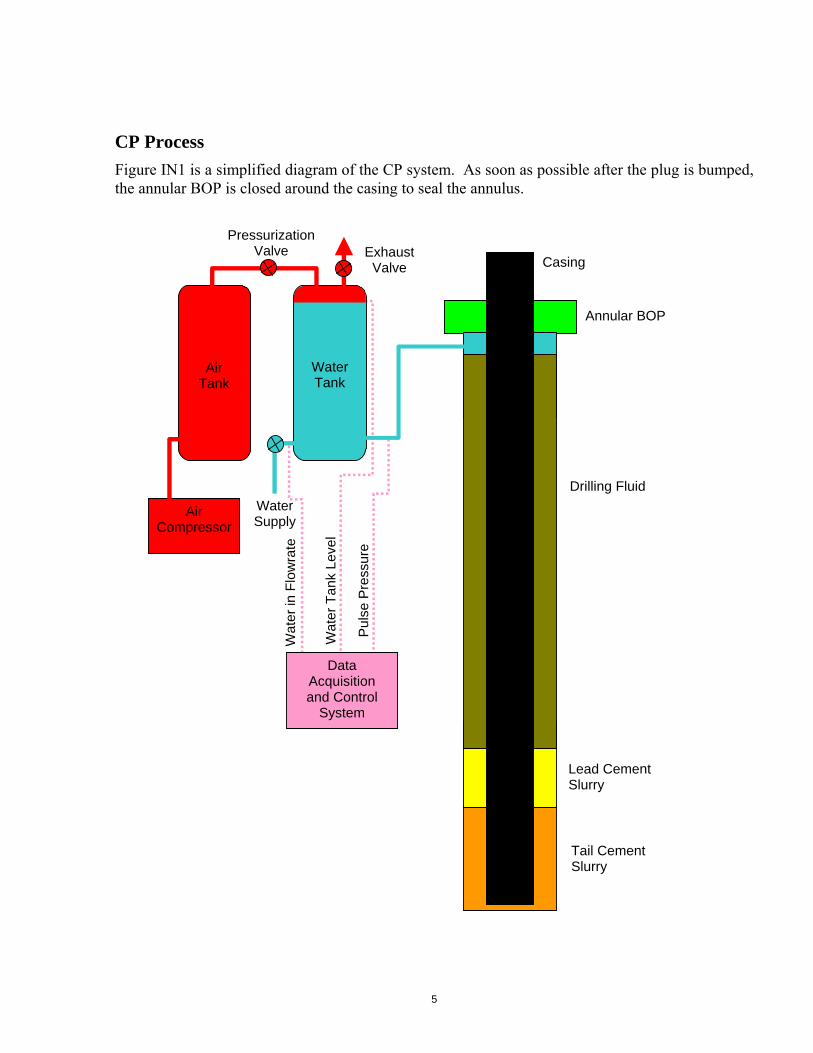
Figure IN1 is a simplified diagram of the CP system. As soon as possible after the plug is bumped, the annular BOP is closed around the casing to seal the annulus.

WaterTank

Air Tank

Annular BOP

Drilling Fluid

Lead Cement Slurry

Tail Cement Slurry

Casing

Air Compressor

Pressurization Valve Exhaust

Valve

Data Acquisition and Control

System

Water Supply

Wat

er T

ank

Leve

l

Wat

er in

Flo

wra

te

Pul

se P

ress

ure

6

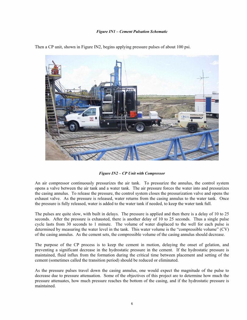
Figure IN1 – Cement Pulsation Schematic

Then a CP unit, shown in Figure IN2, begins applying pressure pulses of about 100 psi.

Figure IN2 – CP Unit with Compressor

An air compressor continuously pressurizes the air tank. To pressurize the annulus, the control system opens a valve between the air tank and a water tank. The air pressure forces the water into and pressurizes the casing annulus. To release the pressure, the control system closes the pressurization valve and opens the exhaust valve. As the pressure is released, water returns from the casing annulus to the water tank. Once the pressure is fully released, water is added to the water tank if needed, to keep the water tank full. The pulses are quite slow, with built in delays. The pressure is applied and then there is a delay of 10 to 25 seconds. After the pressure is exhausted, there is another delay of 10 to 25 seconds. Thus a single pulse cycle lasts from 30 seconds to 1 minute. The volume of water displaced to the well for each pulse is determined by measuring the water level in the tank. This water volume is the “compressible volume” (CV) of the casing annulus. As the cement sets, the compressible volume of the casing annulus should decrease. The purpose of the CP process is to keep the cement in motion, delaying the onset of gelation, and preventing a significant decrease in the hydrostatic pressure in the cement. If the hydrostatic pressure is maintained, fluid influx from the formation during the critical time between placement and setting of the cement (sometimes called the transition period) should be reduced or eliminated. As the pressure pulses travel down the casing annulus, one would expect the magnitude of the pulse to decrease due to pressure attenuation. Some of the objectives of this project are to determine how much the pressure attenuates, how much pressure reaches the bottom of the casing, and if the hydrostatic pressure is maintained.

7

Task List

The CP project completed the following tasks: 1. Characterize the nature of gas migration and the technical and economic problems it causes. [CSI] 2. Identify cultural, technical, and economic barriers to commercialization of CP technology. [Gelb

Consulting Group] 3. Determine the effects of pressure pulses on the cement sheath’s ability to control vertical movement

of gas. [CSI] 4. Develop a self-contained CP system with an electronic data acquisition system (DAS). [CTES] 5. Develop tools, procedures, mathematical models and analysis techniques for monitoring downhole

cement slurry movement and properties using the CP system. [CTES and Griffin] 6. Perform field-testing and evaluation to determine the operating limits and performance capabilities

of the CP technology. [CTES and Griffin] 7. Perform field-testing with downhole measurements. [CTES and Griffin] 8. Determine the effectiveness of CP for preventing gas migration. [CTES] 9. Methods and mathematical models for CP design and control. [LSU] 10. Diagnostic model and analysis method for monitoring pressure pulse transmission and quality of CP

treatment. [LSU] 11. Laboratory procedure for testing cement slurry properties needed for CV design, monitoring and

diagnosis. [LSU] 12. Transfer CP technology to industry. [All Participants]

8

TASK 1 - GAS MIGRATION AND THE PROBLEMS IT CAUSES

A 1995 study by Westport Technology revealed that 15% of primary cement jobs fail, and these cementing problems cost oil and gas producing companies about $470MM annually. Approximately one-third of these problems is attributable to gas migration or formation water flow during placement and curing of the cement in the wellbore. Approximately one-third of these problems are attributable to gas migration or formation water flow during placement and transition of the cement to set. In the 1990’s John Haberman of Texaco E&P proposed applying pressure pulses to the casing annulus above the cement to delay the onset of cement gelation and maintain the hydrostatic pressure. If the hydrostatic pressure is maintained, formation fluid influx during the cement transition period should be eliminated.

9

TASK 2 – IDENTIFICATION OF MARKET BARRIERS

Gelb Consulting Group, Inc. were hired to perform a study of the potential CP market. The objectives of this market study were to determine:

What are the barriers and facilitators to a successful market entry? How attractive are the potential applications? What is the price sensitivity for the cement vibration service?

The study method was:

Phase One: Personal interviews with 8 cementing specialists and one service company o Fred Sabins of Benchmark Research attended all interviews

Phase Two: 51 telephone interviews with cementing specialists and drilling personnel who have significant cementing experience

o Cementing specialists had worldwide responsibility o Drilling personnel had primarily North America responsibility

Respondents were told that this was a new technology from Texaco and shown a brief presentation o See the Appendix for a copy of the questionnaire

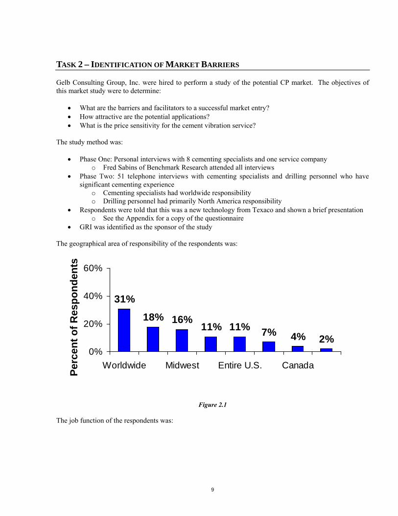
GRI was identified as the sponsor of the study The geographical area of responsibility of the respondents was:

Figure 2.1

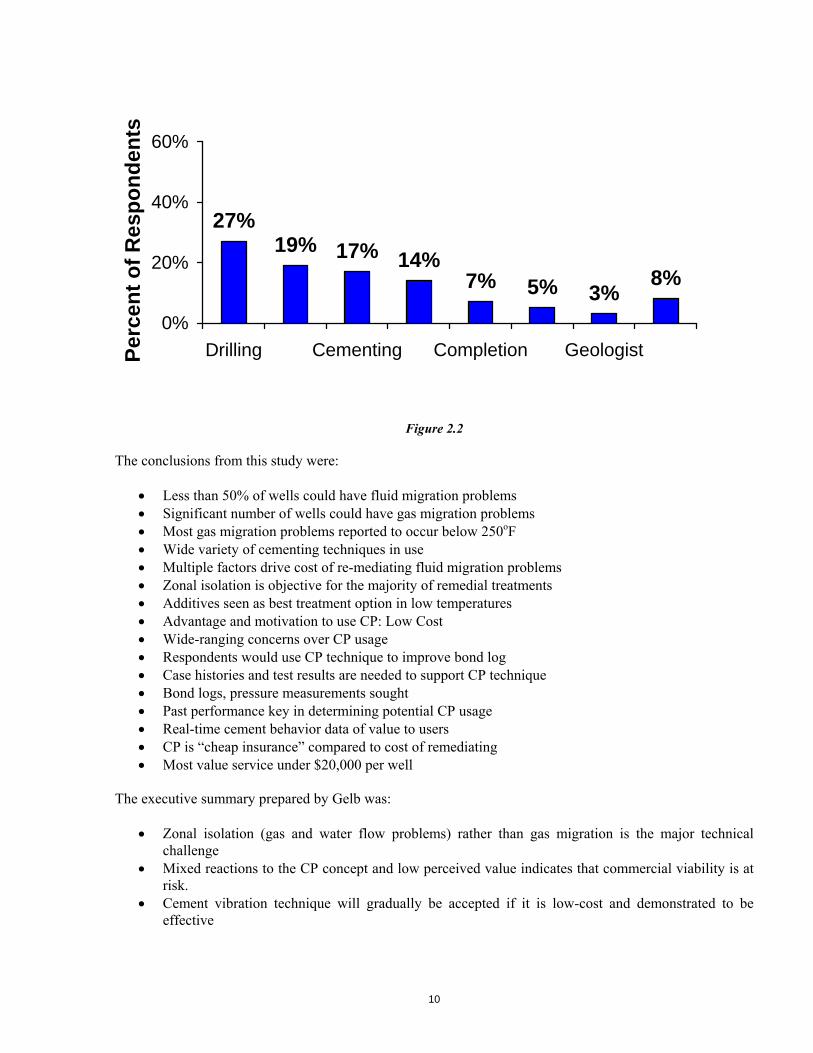
The job function of the respondents was:

31%

18% 16%11% 11% 7% 4% 2%

0%

20%

40%

60%

Worldwide Midwest Entire U.S. Canada

Per

cen

t o

f R

esp

on

den

ts

10

Figure 2.2

The conclusions from this study were:

Less than 50% of wells could have fluid migration problems Significant number of wells could have gas migration problems Most gas migration problems reported to occur below 250oF Wide variety of cementing techniques in use Multiple factors drive cost of re-mediating fluid migration problems Zonal isolation is objective for the majority of remedial treatments Additives seen as best treatment option in low temperatures Advantage and motivation to use CP: Low Cost Wide-ranging concerns over CP usage Respondents would use CP technique to improve bond log Case histories and test results are needed to support CP technique Bond logs, pressure measurements sought Past performance key in determining potential CP usage Real-time cement behavior data of value to users CP is “cheap insurance” compared to cost of remediating Most value service under $20,000 per well

The executive summary prepared by Gelb was:

Zonal isolation (gas and water flow problems) rather than gas migration is the major technical challenge

Mixed reactions to the CP concept and low perceived value indicates that commercial viability is at risk.

Cement vibration technique will gradually be accepted if it is low-cost and demonstrated to be effective

27%19% 17% 14%

7% 5% 3%8%

0%

20%

40%

60%

Drilling Cementing Completion GeologistPer

cen

t o

f R

esp

on

den

ts

11

o Buyers want test results and case histories documenting successes of the cement vibration technique

o Improved cement bond log seen as a valuable reason to use the service o CP must become part of “standard cementing practice” to gain widespread acceptance. This

means CP must work regardless of the slurry design. o Cementing service company resistance at the district level may slow market acceptance o Price point should be under $5,000 per job.

For more details see the full report from Gelb in GRI report number GRI-01/0179.2.

12

TASK 3 - DETERMINE THE EFFECT OF CP ON THE CEMENT SHEATH

The purpose of this task of the Pulsation project was to determine the effects of pressure pulses through unset cement upon shear bond of the cement to pipe and compressive strength. One specific cement composition was tested in the pulsation test model. Pressure pulses were generated through the cement at two different displacements and velocities until the cement samples reached sufficient strength to resist at least 100-psi differential pressure (pulse test 3 could not be pulsed more than 74-psi because the differential pressure just leveled out). The 100-psi differential pressure corresponds to a static gel strength of 13,125-lbs/100 ft2. This is significantly higher than static gel strength equivalent to initial set (1,500 lbs/100ft2). This value was chosen to intentionally simulate a worst-case condition. After additional static cure time both “shear bond” and “compressive strength” measurements were conducted on the set cement. From the data generated in this task of the Pulsation project it is apparent that the effect of pulsation on the properties of cement systems are not significant. The data from this task illustrates this even though the cement slurries were intentionally pulsed past maximum static gel strength and compressive strength initial set. The pulsation does not produce lower shear bonds or compressive strengths than the comparison slurries that were not pulsed. The final report from CSI, which discusses testing program details and results, is included in report GRI-01/0179.2.

13

TASK 4 - DEVELOPMENT OF A SELF-CONTAINED CP UNIT (CPU)

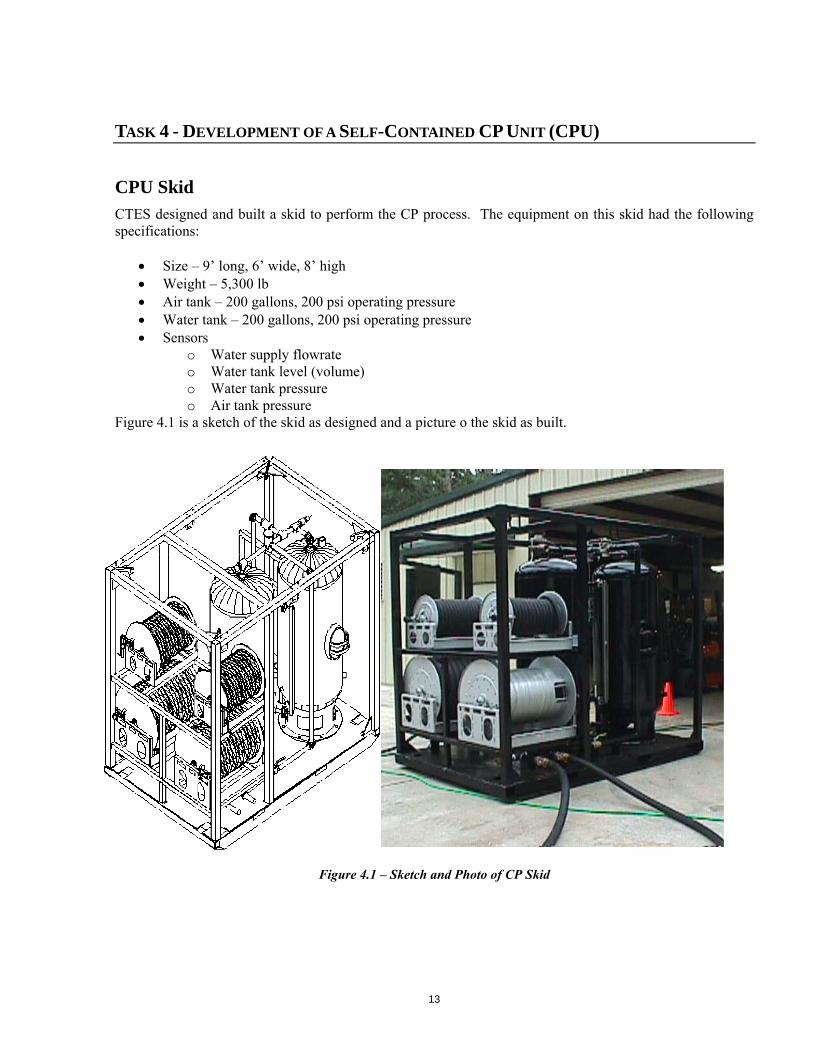
CPU Skid CTES designed and built a skid to perform the CP process. The equipment on this skid had the following specifications:

Size – 9’ long, 6’ wide, 8’ high Weight – 5,300 lb Air tank – 200 gallons, 200 psi operating pressure Water tank – 200 gallons, 200 psi operating pressure Sensors

o Water supply flowrate o Water tank level (volume) o Water tank pressure o Air tank pressure

Figure 4.1 is a sketch of the skid as designed and a picture o the skid as built.

Figure 4.1 – Sketch and Photo of CP Skid

14

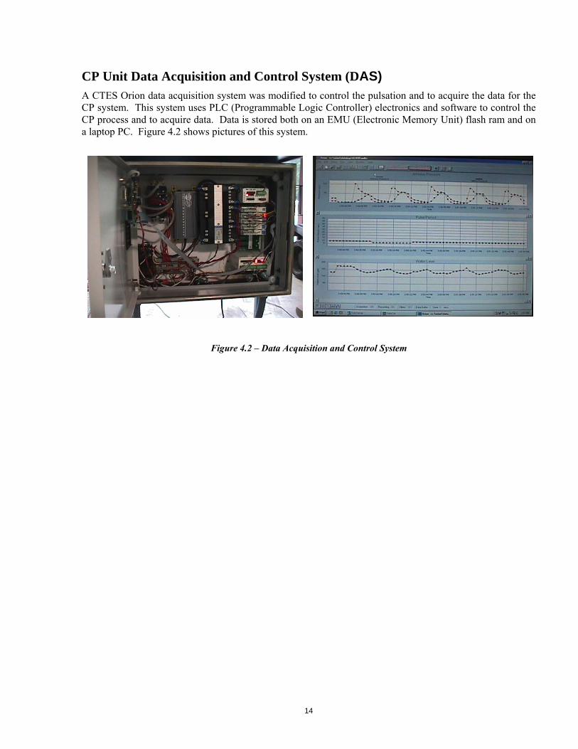
CP Unit Data Acquisition and Control System (DAS) A CTES Orion data acquisition system was modified to control the pulsation and to acquire the data for the CP system. This system uses PLC (Programmable Logic Controller) electronics and software to control the CP process and to acquire data. Data is stored both on an EMU (Electronic Memory Unit) flash ram and on a laptop PC. Figure 4.2 shows pictures of this system.

Figure 4.2 – Data Acquisition and Control System

15

TASK 5- MONITORING TOOLS AND PROCEDURES

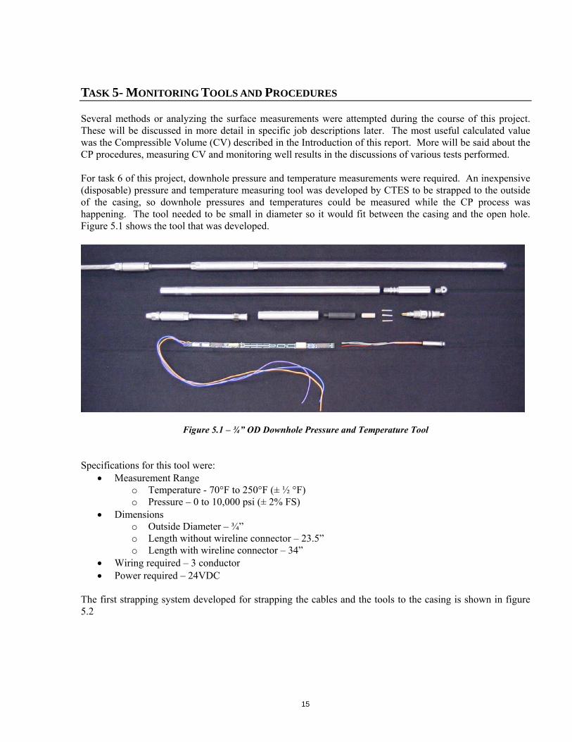
Several methods or analyzing the surface measurements were attempted during the course of this project. These will be discussed in more detail in specific job descriptions later. The most useful calculated value was the Compressible Volume (CV) described in the Introduction of this report. More will be said about the CP procedures, measuring CV and monitoring well results in the discussions of various tests performed. For task 6 of this project, downhole pressure and temperature measurements were required. An inexpensive (disposable) pressure and temperature measuring tool was developed by CTES to be strapped to the outside of the casing, so downhole pressures and temperatures could be measured while the CP process was happening. The tool needed to be small in diameter so it would fit between the casing and the open hole. Figure 5.1 shows the tool that was developed.

Figure 5.1 – ¾” OD Downhole Pressure and Temperature Tool

Specifications for this tool were:

Measurement Range o Temperature - 70°F to 250°F (± ½ °F) o Pressure – 0 to 10,000 psi (± 2% FS)

Dimensions o Outside Diameter – ¾” o Length without wireline connector – 23.5” o Length with wireline connector – 34”

Wiring required – 3 conductor Power required – 24VDC

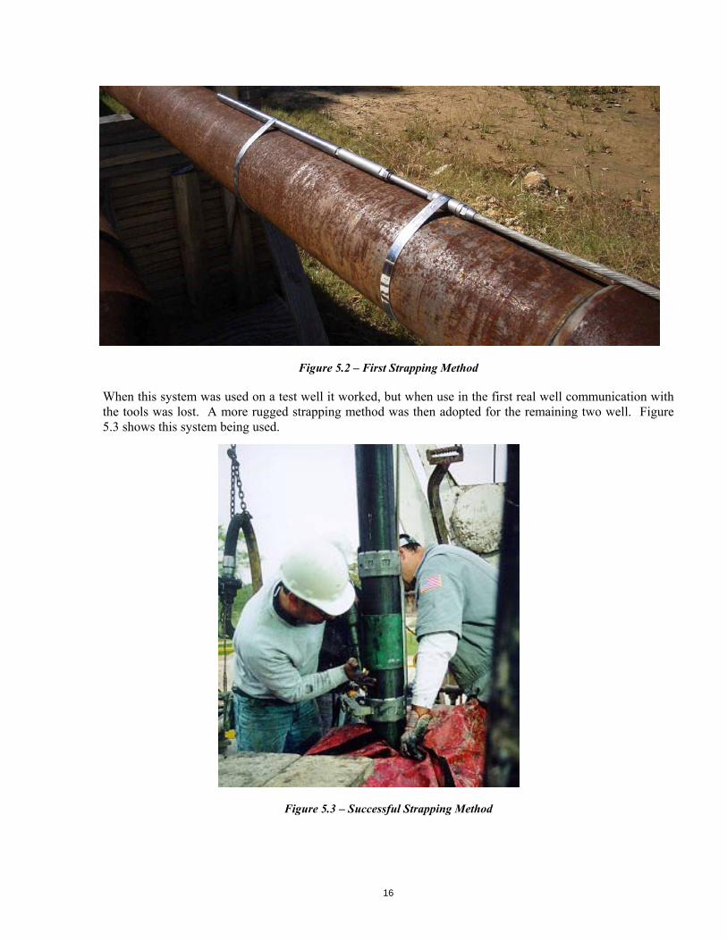
The first strapping system developed for strapping the cables and the tools to the casing is shown in figure 5.2

16

Figure 5.2 – First Strapping Method

When this system was used on a test well it worked, but when use in the first real well communication with the tools was lost. A more rugged strapping method was then adopted for the remaining two well. Figure 5.3 shows this system being used.

Figure 5.3 – Successful Strapping Method

17

TASK 6 – FIELD EVALUATION OF CP

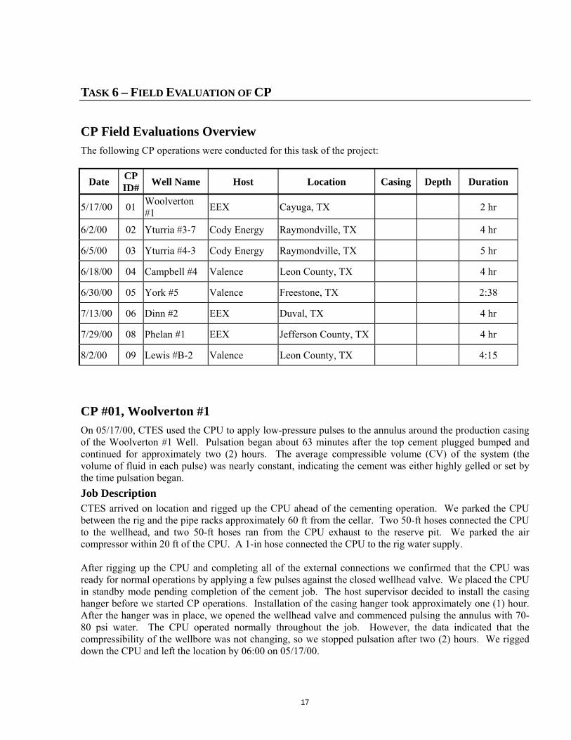
CP Field Evaluations Overview The following CP operations were conducted for this task of the project:

Date CP ID#

Well Name Host Location Casing Depth Duration

5/17/00 01 Woolverton #1

EEX Cayuga, TX 2 hr

6/2/00 02 Yturria #3-7 Cody Energy Raymondville, TX 4 hr

6/5/00 03 Yturria #4-3 Cody Energy Raymondville, TX 5 hr

6/18/00 04 Campbell #4 Valence Leon County, TX 4 hr

6/30/00 05 York #5 Valence Freestone, TX 2:38

7/13/00 06 Dinn #2 EEX Duval, TX 4 hr

7/29/00 08 Phelan #1 EEX Jefferson County, TX 4 hr

8/2/00 09 Lewis #B-2 Valence Leon County, TX 4:15

CP #01, Woolverton #1 On 05/17/00, CTES used the CPU to apply low-pressure pulses to the annulus around the production casing of the Woolverton #1 Well. Pulsation began about 63 minutes after the top cement plugged bumped and continued for approximately two (2) hours. The average compressible volume (CV) of the system (the volume of fluid in each pulse) was nearly constant, indicating the cement was either highly gelled or set by the time pulsation began.

Job Description CTES arrived on location and rigged up the CPU ahead of the cementing operation. We parked the CPU between the rig and the pipe racks approximately 60 ft from the cellar. Two 50-ft hoses connected the CPU to the wellhead, and two 50-ft hoses ran from the CPU exhaust to the reserve pit. We parked the air compressor within 20 ft of the CPU. A 1-in hose connected the CPU to the rig water supply. After rigging up the CPU and completing all of the external connections we confirmed that the CPU was ready for normal operations by applying a few pulses against the closed wellhead valve. We placed the CPU in standby mode pending completion of the cement job. The host supervisor decided to install the casing hanger before we started CP operations. Installation of the casing hanger took approximately one (1) hour. After the hanger was in place, we opened the wellhead valve and commenced pulsing the annulus with 70-80 psi water. The CPU operated normally throughout the job. However, the data indicated that the compressibility of the wellbore was not changing, so we stopped pulsation after two (2) hours. We rigged down the CPU and left the location by 06:00 on 05/17/00.

18

Results

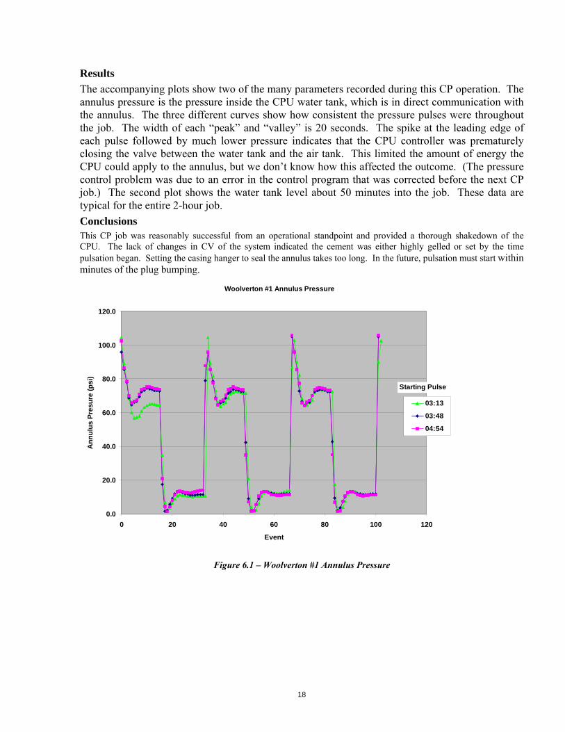
The accompanying plots show two of the many parameters recorded during this CP operation. The annulus pressure is the pressure inside the CPU water tank, which is in direct communication with the annulus. The three different curves show how consistent the pressure pulses were throughout the job. The width of each “peak” and “valley” is 20 seconds. The spike at the leading edge of each pulse followed by much lower pressure indicates that the CPU controller was prematurely closing the valve between the water tank and the air tank. This limited the amount of energy the CPU could apply to the annulus, but we don’t know how this affected the outcome. (The pressure control problem was due to an error in the control program that was corrected before the next CP job.) The second plot shows the water tank level about 50 minutes into the job. These data are typical for the entire 2-hour job.

Conclusions This CP job was reasonably successful from an operational standpoint and provided a thorough shakedown of the CPU. The lack of changes in CV of the system indicated the cement was either highly gelled or set by the time pulsation began. Setting the casing hanger to seal the annulus takes too long. In the future, pulsation must start within minutes of the plug bumping.

Figure 6.1 – Woolverton #1 Annulus Pressure

Woolverton #1 Annulus Pressure

0.0

20.0

40.0

60.0

80.0

100.0

120.0

0 20 40 60 80 100 120

Event

An

nu

lus

Pre

sure

(p

si)

03:13

03:48

04:54

Starting Pulse

19

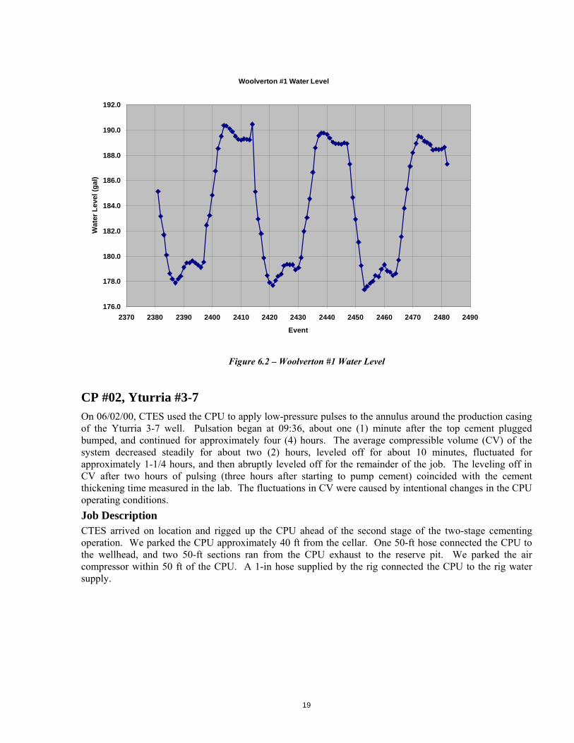
Figure 6.2 – Woolverton #1 Water Level

CP #02, Yturria #3-7 On 06/02/00, CTES used the CPU to apply low-pressure pulses to the annulus around the production casing of the Yturria 3-7 well. Pulsation began at 09:36, about one (1) minute after the top cement plugged bumped, and continued for approximately four (4) hours. The average compressible volume (CV) of the system decreased steadily for about two (2) hours, leveled off for about 10 minutes, fluctuated for approximately 1-1/4 hours, and then abruptly leveled off for the remainder of the job. The leveling off in CV after two hours of pulsing (three hours after starting to pump cement) coincided with the cement thickening time measured in the lab. The fluctuations in CV were caused by intentional changes in the CPU operating conditions.

Job Description CTES arrived on location and rigged up the CPU ahead of the second stage of the two-stage cementing operation. We parked the CPU approximately 40 ft from the cellar. One 50-ft hose connected the CPU to the wellhead, and two 50-ft sections ran from the CPU exhaust to the reserve pit. We parked the air compressor within 50 ft of the CPU. A 1-in hose supplied by the rig connected the CPU to the rig water supply.

Woolverton #1 Water Level

176.0

178.0

180.0

182.0

184.0

186.0

188.0

190.0

192.0

2370 2380 2390 2400 2410 2420 2430 2440 2450 2460 2470 2480 2490

Event

Wat

er L

evel

(g

al)

20

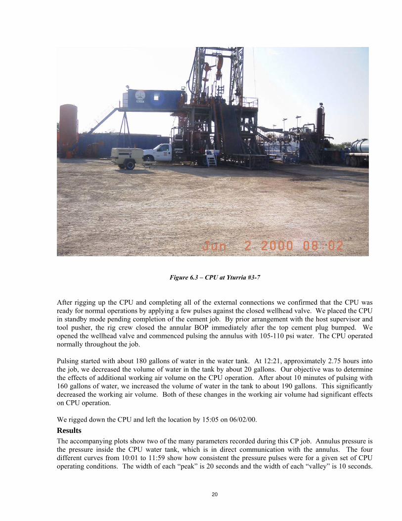
Figure 6.3 – CPU at Yturria #3-7

After rigging up the CPU and completing all of the external connections we confirmed that the CPU was ready for normal operations by applying a few pulses against the closed wellhead valve. We placed the CPU in standby mode pending completion of the cement job. By prior arrangement with the host supervisor and tool pusher, the rig crew closed the annular BOP immediately after the top cement plug bumped. We opened the wellhead valve and commenced pulsing the annulus with 105-110 psi water. The CPU operated normally throughout the job. Pulsing started with about 180 gallons of water in the water tank. At 12:21, approximately 2.75 hours into the job, we decreased the volume of water in the tank by about 20 gallons. Our objective was to determine the effects of additional working air volume on the CPU operation. After about 10 minutes of pulsing with 160 gallons of water, we increased the volume of water in the tank to about 190 gallons. This significantly decreased the working air volume. Both of these changes in the working air volume had significant effects on CPU operation. We rigged down the CPU and left the location by 15:05 on 06/02/00.

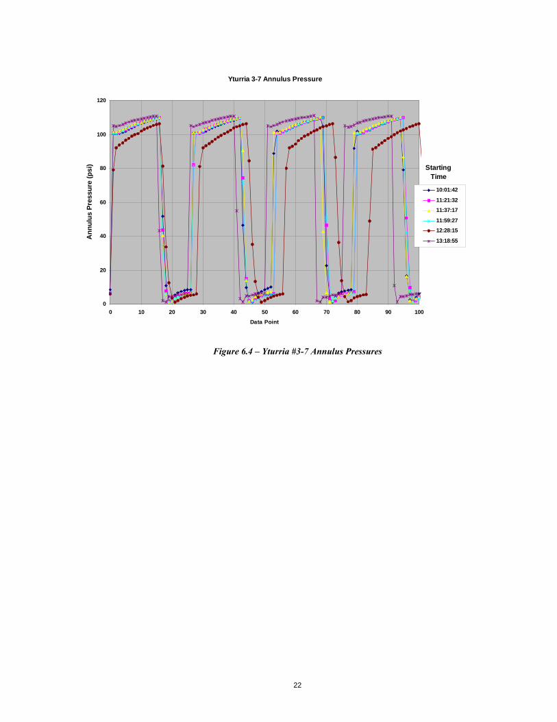
Results The accompanying plots show two of the many parameters recorded during this CP job. Annulus pressure is the pressure inside the CPU water tank, which is in direct communication with the annulus. The four different curves from 10:01 to 11:59 show how consistent the pressure pulses were for a given set of CPU operating conditions. The width of each “peak” is 20 seconds and the width of each “valley” is 10 seconds.

21

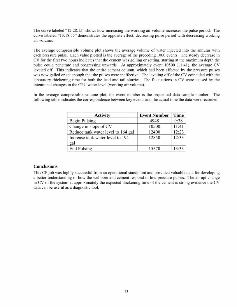
The curve labeled “12:28:15” shows how increasing the working air volume increases the pulse period. The curve labeled “13:18:55” demonstrates the opposite effect; decreasing pulse period with decreasing working air volume. The average compressible volume plot shows the average volume of water injected into the annulus with each pressure pulse. Each value plotted is the average of the preceding 1000 events. The steady decrease in CV for the first two hours indicates that the cement was gelling or setting, starting at the maximum depth the pulse could penetrate and progressing upwards. At approximately event 10500 (11:41), the average CV leveled off. This indicates that the entire cement column, which had been affected by the pressure pulses was now gelled or set enough that the pulses were ineffective. The leveling off of the CV coincided with the laboratory thickening time for both the lead and tail slurries. The fluctuations in CV were caused by the intentional changes in the CPU water level (working air volume). In the average compressible volume plot, the event number is the sequential data sample number. The following table indicates the correspondence between key events and the actual time the data were recorded.

Activity Event Number Time Begin Pulsing 4948 9:38 Change in slope of CV 10500 11:41 Reduce tank water level to 164 gal 12400 12:23 Increase tank water level to 194 gal

12850 12:33

End Pulsing 15570 13:33

Conclusions This CP job was highly successful from an operational standpoint and provided valuable data for developing a better understanding of how the wellbore and cement respond to low-pressure pulses. The abrupt change in CV of the system at approximately the expected thickening time of the cement is strong evidence the CV data can be useful as a diagnostic tool.

22

Figure 6.4 – Yturria #3-7 Annulus Pressures

Yturria 3-7 Annulus Pressure

0

20

40

60

80

100

120

0 10 20 30 40 50 60 70 80 90 100

Data Point

An

nu

lus

Pre

ssu

re (

psi

)

10:01:42

11:21:32

11:37:17

11:59:27

12:28:15

13:18:55

Starting Time

23

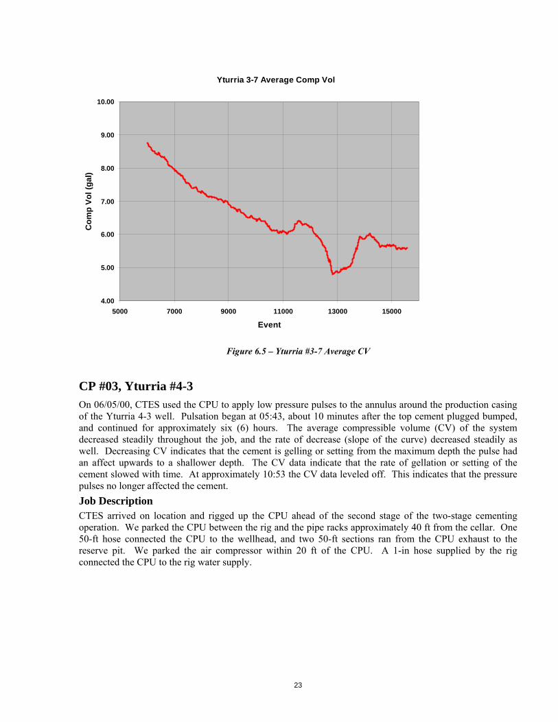
Figure 6.5 – Yturria #3-7 Average CV

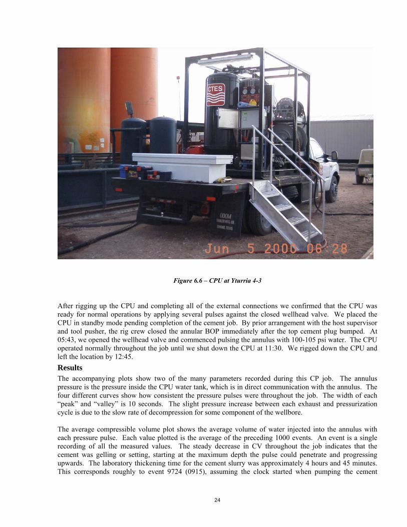
CP #03, Yturria #4-3 On 06/05/00, CTES used the CPU to apply low pressure pulses to the annulus around the production casing of the Yturria 4-3 well. Pulsation began at 05:43, about 10 minutes after the top cement plugged bumped, and continued for approximately six (6) hours. The average compressible volume (CV) of the system decreased steadily throughout the job, and the rate of decrease (slope of the curve) decreased steadily as well. Decreasing CV indicates that the cement is gelling or setting from the maximum depth the pulse had an affect upwards to a shallower depth. The CV data indicate that the rate of gellation or setting of the cement slowed with time. At approximately 10:53 the CV data leveled off. This indicates that the pressure pulses no longer affected the cement.

Job Description CTES arrived on location and rigged up the CPU ahead of the second stage of the two-stage cementing operation. We parked the CPU between the rig and the pipe racks approximately 40 ft from the cellar. One 50-ft hose connected the CPU to the wellhead, and two 50-ft sections ran from the CPU exhaust to the reserve pit. We parked the air compressor within 20 ft of the CPU. A 1-in hose supplied by the rig connected the CPU to the rig water supply.

Yturria 3-7 Average Comp Vol

4.00

5.00

6.00

7.00

8.00

9.00

10.00

5000 7000 9000 11000 13000 15000

Event

Co

mp

Vo

l (g

al)

24

Figure 6.6 – CPU at Yturria 4-3

After rigging up the CPU and completing all of the external connections we confirmed that the CPU was ready for normal operations by applying several pulses against the closed wellhead valve. We placed the CPU in standby mode pending completion of the cement job. By prior arrangement with the host supervisor and tool pusher, the rig crew closed the annular BOP immediately after the top cement plug bumped. At 05:43, we opened the wellhead valve and commenced pulsing the annulus with 100-105 psi water. The CPU operated normally throughout the job until we shut down the CPU at 11:30. We rigged down the CPU and left the location by 12:45.

Results The accompanying plots show two of the many parameters recorded during this CP job. The annulus pressure is the pressure inside the CPU water tank, which is in direct communication with the annulus. The four different curves show how consistent the pressure pulses were throughout the job. The width of each “peak” and “valley” is 10 seconds. The slight pressure increase between each exhaust and pressurization cycle is due to the slow rate of decompression for some component of the wellbore. The average compressible volume plot shows the average volume of water injected into the annulus with each pressure pulse. Each value plotted is the average of the preceding 1000 events. An event is a single recording of all the measured values. The steady decrease in CV throughout the job indicates that the cement was gelling or setting, starting at the maximum depth the pulse could penetrate and progressing upwards. The laboratory thickening time for the cement slurry was approximately 4 hours and 45 minutes. This corresponds roughly to event 9724 (0915), assuming the clock started when pumping the cement

25

commenced. At approximately event 14000 (10:53), the average CV leveled off. This indicates that the entire cement column, which had been affected by the pressure pulses was now gelled or set enough that the pulses were ineffective. The following table shows the correspondence between selected event numbers and clock time.

Activity Event Number TimeBegin pulsing 186 05:43Thickening time 9724 09:15CV leveling off 14000 10:53End pulsing 16029 11:34

Conclusions This CP job was highly successful from an operational standpoint and provided valuable data for developing a better understanding of how the wellbore and cement respond to low-pressure pulses.

Figure 6.7 – Yturria #4-3 Annulus Pressures

Yturria 4-3 Annulus Pressures

0

20

40

60

80

100

120

0 10 20 30 40 50 60 70 80

Data Point

An

nu

lus

Pre

ssu

re (

psi

)

06:45

07:30

08:59

10:27

Starting Time

26

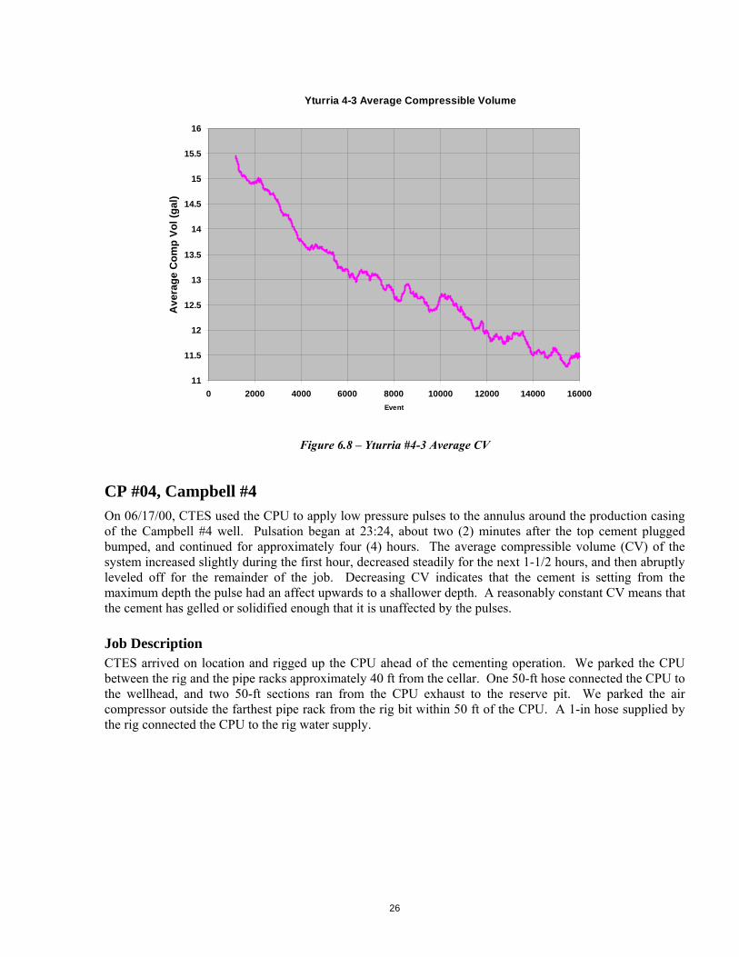
Figure 6.8 – Yturria #4-3 Average CV

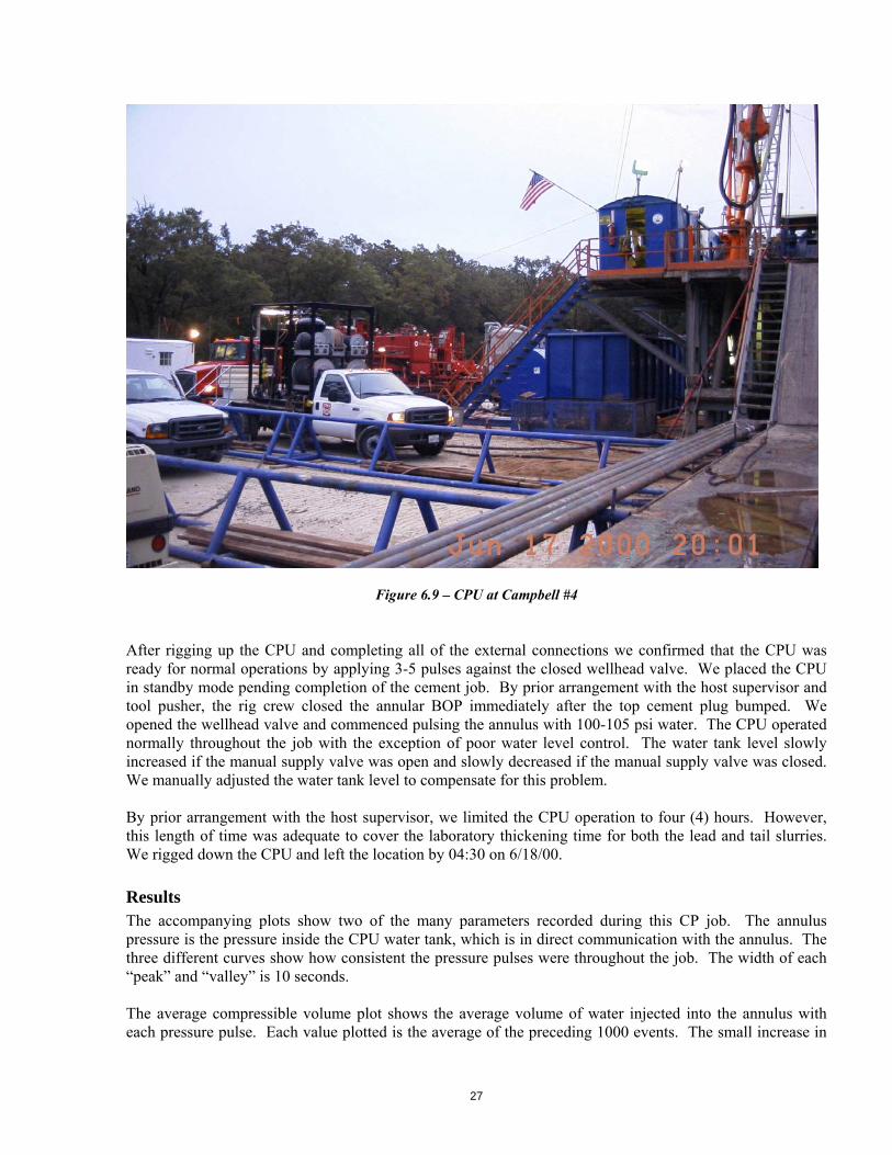
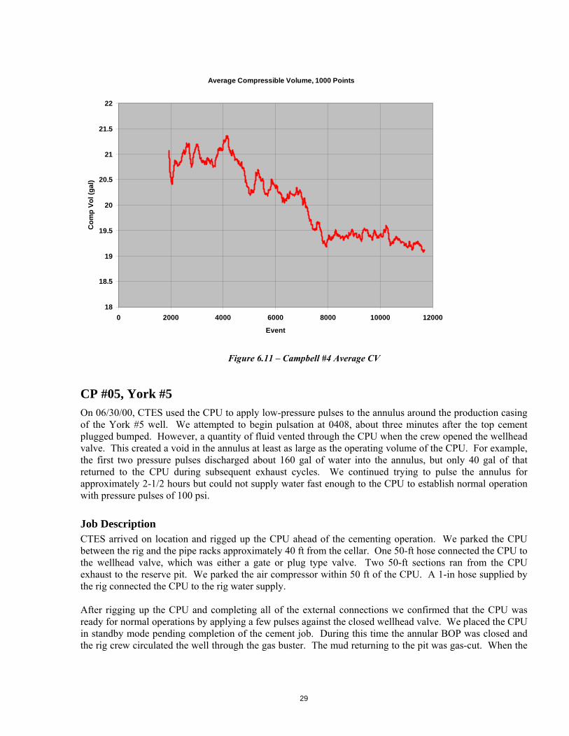
CP #04, Campbell #4 On 06/17/00, CTES used the CPU to apply low pressure pulses to the annulus around the production casing of the Campbell #4 well. Pulsation began at 23:24, about two (2) minutes after the top cement plugged bumped, and continued for approximately four (4) hours. The average compressible volume (CV) of the system increased slightly during the first hour, decreased steadily for the next 1-1/2 hours, and then abruptly leveled off for the remainder of the job. Decreasing CV indicates that the cement is setting from the maximum depth the pulse had an affect upwards to a shallower depth. A reasonably constant CV means that the cement has gelled or solidified enough that it is unaffected by the pulses.

Job Description CTES arrived on location and rigged up the CPU ahead of the cementing operation. We parked the CPU between the rig and the pipe racks approximately 40 ft from the cellar. One 50-ft hose connected the CPU to the wellhead, and two 50-ft sections ran from the CPU exhaust to the reserve pit. We parked the air compressor outside the farthest pipe rack from the rig bit within 50 ft of the CPU. A 1-in hose supplied by the rig connected the CPU to the rig water supply.

Yturria 4-3 Average Compressible Volume

11

11.5

12

12.5

13

13.5

14

14.5

15

15.5

16

0 2000 4000 6000 8000 10000 12000 14000 16000

Event

Av

era

ge

Co

mp

Vo

l (g

al)

27

Figure 6.9 – CPU at Campbell #4

After rigging up the CPU and completing all of the external connections we confirmed that the CPU was ready for normal operations by applying 3-5 pulses against the closed wellhead valve. We placed the CPU in standby mode pending completion of the cement job. By prior arrangement with the host supervisor and tool pusher, the rig crew closed the annular BOP immediately after the top cement plug bumped. We opened the wellhead valve and commenced pulsing the annulus with 100-105 psi water. The CPU operated normally throughout the job with the exception of poor water level control. The water tank level slowly increased if the manual supply valve was open and slowly decreased if the manual supply valve was closed. We manually adjusted the water tank level to compensate for this problem. By prior arrangement with the host supervisor, we limited the CPU operation to four (4) hours. However, this length of time was adequate to cover the laboratory thickening time for both the lead and tail slurries. We rigged down the CPU and left the location by 04:30 on 6/18/00.

Results The accompanying plots show two of the many parameters recorded during this CP job. The annulus pressure is the pressure inside the CPU water tank, which is in direct communication with the annulus. The three different curves show how consistent the pressure pulses were throughout the job. The width of each “peak” and “valley” is 10 seconds. The average compressible volume plot shows the average volume of water injected into the annulus with each pressure pulse. Each value plotted is the average of the preceding 1000 events. The small increase in

28

CV during the first hour (2000 events » 0.75 hr) may indicate that the pulses were able to break the gel structure in the cement column to some depth. The steady decrease in CV for the next 1-1/2 hours indicates that the cement was gelling or setting, starting at the maximum depth the pulse could penetrate and progressing upwards. At approximately event 8000 (02:06), the average CV leveled off. This indicates that the entire cement column, which had been affected by the pressure pulses was now gelled or set enough that the pulses were ineffective. The laboratory thickening time for both the lead and tail slurries was approximately 3 hours and 20 minutes. This corresponds roughly to event 7435, assuming the clock started when pumping the cement commenced.

Conclusions This CP job was highly successful from an operational standpoint and provided valuable data for developing a better understanding of how the wellbore and cement respond to low pressure pulses. The abrupt change in CV of the system at approximately the expected thickening time of the cement is strong evidence the CV data can be useful as a diagnostic tool.

Figure 6.10 – Campbell #4 Annulus Pressures

Annulus Pressure

0

20

40

60

80

100

120

0 10 20 30 40 50 60 70

Data Point

An

nu

lus

Pre

ssu

re (

psi

)

2000

6000

10,000

FirstEvent

29

Figure 6.11 – Campbell #4 Average CV

CP #05, York #5 On 06/30/00, CTES used the CPU to apply low-pressure pulses to the annulus around the production casing of the York #5 well. We attempted to begin pulsation at 0408, about three minutes after the top cement plugged bumped. However, a quantity of fluid vented through the CPU when the crew opened the wellhead valve. This created a void in the annulus at least as large as the operating volume of the CPU. For example, the first two pressure pulses discharged about 160 gal of water into the annulus, but only 40 gal of that returned to the CPU during subsequent exhaust cycles. We continued trying to pulse the annulus for approximately 2-1/2 hours but could not supply water fast enough to the CPU to establish normal operation with pressure pulses of 100 psi.

Job Description CTES arrived on location and rigged up the CPU ahead of the cementing operation. We parked the CPU between the rig and the pipe racks approximately 40 ft from the cellar. One 50-ft hose connected the CPU to the wellhead valve, which was either a gate or plug type valve. Two 50-ft sections ran from the CPU exhaust to the reserve pit. We parked the air compressor within 50 ft of the CPU. A 1-in hose supplied by the rig connected the CPU to the rig water supply. After rigging up the CPU and completing all of the external connections we confirmed that the CPU was ready for normal operations by applying a few pulses against the closed wellhead valve. We placed the CPU in standby mode pending completion of the cement job. During this time the annular BOP was closed and the rig crew circulated the well through the gas buster. The mud returning to the pit was gas-cut. When the

Average Compressible Volume, 1000 Points

18

18.5

19

19.5

20

20.5

21

21.5

22

0 2000 4000 6000 8000 10000 12000

Event

Co

mp

Vo

l (g

al)

30

gas content of the mud returns decreased to a level acceptable to the host supervisor, the cementing operation started. The annular BOP remained closed during the cementing operation and the CP operation. We opened the wellhead valve about three minutes after the plug bumped and attempted to start pulsing the annulus with 100-105 psi water. However a quantity of fluid from the annulus vented through the CPU before the pressurization cycle started. This created a void in the annulus at least as large as the operating volume of the CPU. For example, the first two pressure pulses discharged about 160 gal of water into the annulus, but only 40 gal of that returned to the CPU during subsequent exhaust cycles. We continued trying to pulse the annulus for approximately 2-1/2 hours but could not supply water fast enough to the CPU to establish normal operation with pressure pulses of 100 psi.

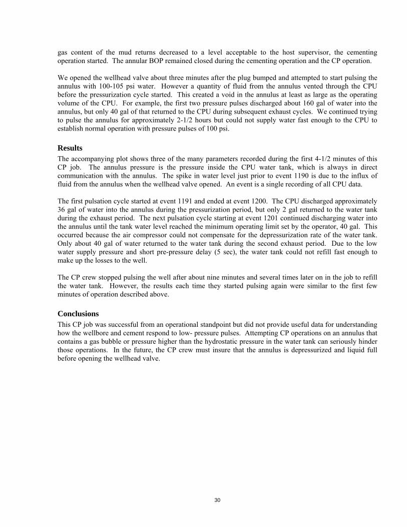
Results The accompanying plot shows three of the many parameters recorded during the first 4-1/2 minutes of this CP job. The annulus pressure is the pressure inside the CPU water tank, which is always in direct communication with the annulus. The spike in water level just prior to event 1190 is due to the influx of fluid from the annulus when the wellhead valve opened. An event is a single recording of all CPU data. The first pulsation cycle started at event 1191 and ended at event 1200. The CPU discharged approximately 36 gal of water into the annulus during the pressurization period, but only 2 gal returned to the water tank during the exhaust period. The next pulsation cycle starting at event 1201 continued discharging water into the annulus until the tank water level reached the minimum operating limit set by the operator, 40 gal. This occurred because the air compressor could not compensate for the depressurization rate of the water tank. Only about 40 gal of water returned to the water tank during the second exhaust period. Due to the low water supply pressure and short pre-pressure delay (5 sec), the water tank could not refill fast enough to make up the losses to the well. The CP crew stopped pulsing the well after about nine minutes and several times later on in the job to refill the water tank. However, the results each time they started pulsing again were similar to the first few minutes of operation described above.

Conclusions This CP job was successful from an operational standpoint but did not provide useful data for understanding how the wellbore and cement respond to low- pressure pulses. Attempting CP operations on an annulus that contains a gas bubble or pressure higher than the hydrostatic pressure in the water tank can seriously hinder those operations. In the future, the CP crew must insure that the annulus is depressurized and liquid full before opening the wellhead valve.

31

Figure 6.12 – York #5 Operating Data

CP #06, Dinn #2 On 07/13/00, CTES used the CPU to apply low-pressure pulses to the annulus around the production casing of the Dinn #2 well. This was the deepest well attempted to date and the first job with oil-based mud in the annulus. Pulsation began about 10 minutes after the top cement plugged bumped and continued for approximately four (4) hours. The average compressible volume (CV) of the system (the volume of fluid in each pulse) decreased slightly during this time but did not indicate any distinctive change in the cement gel strength. The tall column (11,495 ft) of 17 ppg oil-based mud may have attenuated the 105 psi pressure pulses or masked the response of the relatively short (2600 ft) column of cement.

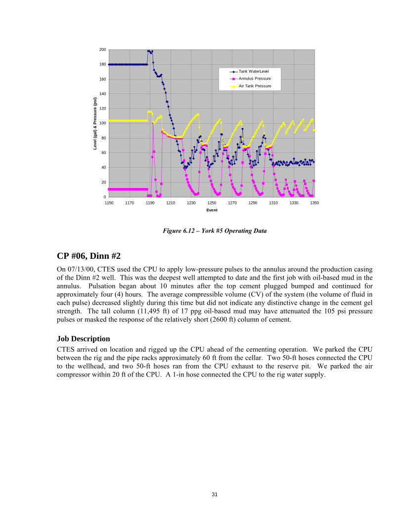
Job Description CTES arrived on location and rigged up the CPU ahead of the cementing operation. We parked the CPU between the rig and the pipe racks approximately 60 ft from the cellar. Two 50-ft hoses connected the CPU to the wellhead, and two 50-ft hoses ran from the CPU exhaust to the reserve pit. We parked the air compressor within 20 ft of the CPU. A 1-in hose connected the CPU to the rig water supply.

0

20

40

60

80

100

120

140

160

180

200

1150 1170 1190 1210 1230 1250 1270 1290 1310 1330 1350

Event

Lev

el (

gal

) &

Pre

ssu

re (

psi

)

Tank WaterLevel

Annulus Pressure

Air Tank Pressure

32

Figure 6.13 – CPU at Dinn #2

After rigging up the CPU and completing all of the external connections we confirmed that the CPU was ready for normal operations by applying a few pulses against the closed wellhead valve. We placed the CPU in standby mode pending completion of the cement job. By prior arrangement with the host supervisor and tool pusher, the rig crew closed the BOP pipe rams shortly after the top cement plug bumped. At 20:02, we opened the wellhead valve and commenced pulsing the annulus with 105-110 psi water. The CPU operated normally, but the water tank level slowly increased throughout the job due to flow from the well. This flow decreased from about 0.3 gpm to 0.1 gpm during the job and was probably due to thermal expansion of the oil-based mud. We manually released the extra volume at several times during the job in order to keep the water tank from overflowing. The CPU data indicated that the compressibility of the wellbore was not changing, so we stopped pulsation after four (4) hours. We rigged down the CPU and left the location by 01:00 on 07/14/00.

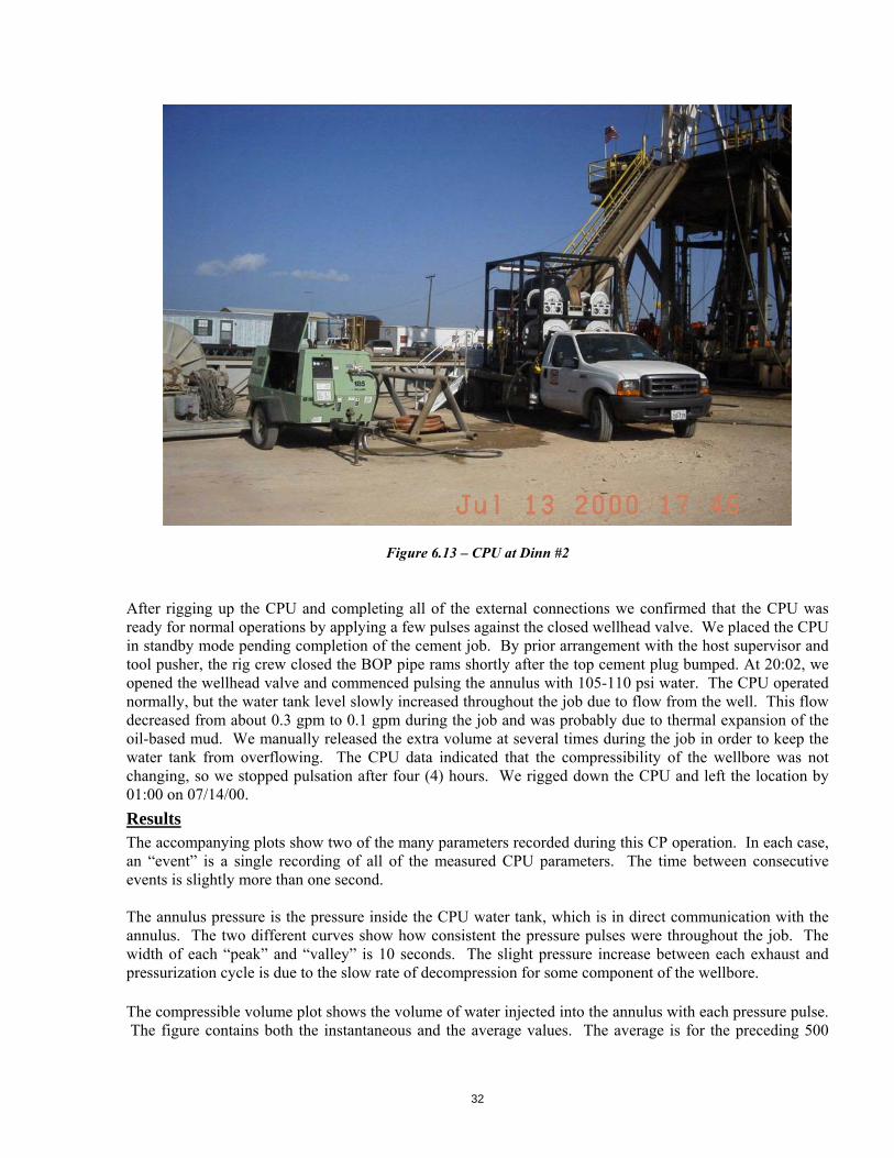
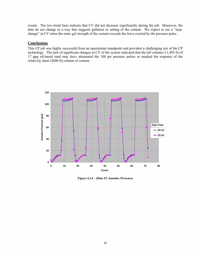
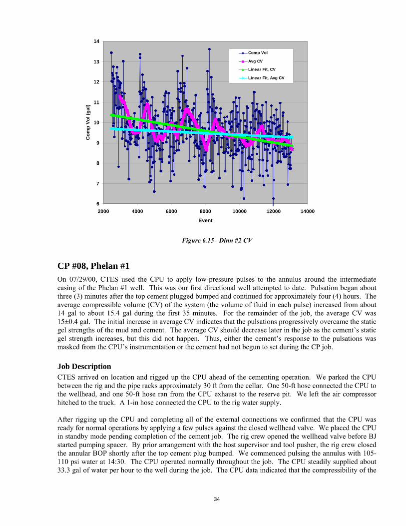
Results The accompanying plots show two of the many parameters recorded during this CP operation. In each case, an “event” is a single recording of all of the measured CPU parameters. The time between consecutive events is slightly more than one second. The annulus pressure is the pressure inside the CPU water tank, which is in direct communication with the annulus. The two different curves show how consistent the pressure pulses were throughout the job. The width of each “peak” and “valley” is 10 seconds. The slight pressure increase between each exhaust and pressurization cycle is due to the slow rate of decompression for some component of the wellbore. The compressible volume plot shows the volume of water injected into the annulus with each pressure pulse. The figure contains both the instantaneous and the average values. The average is for the preceding 500

33

events. The two trend lines indicate that CV did not decrease significantly during the job. Moreover, the data do not change in a way that suggests gellation or setting of the cement. We expect to see a “step-change” in CV when the static gel strength of the cement exceeds the force exerted by the pressure pulse.

Conclusions This CP job was highly successful from an operational standpoint and provided a challenging test of the CP technology. The lack of significant changes in CV of the system indicated that the tall column (11,495 ft) of 17 ppg oil-based mud may have attenuated the 100 psi pressure pulses or masked the response of the relatively short (2600 ft) column of cement.

Figure 6.14 – Dinn #2 Annulus Pressures

0

20

40

60

80

100

120

0 10 20 30 40 50 60 70 80

Event

An

nu

lus

Pre

ssu

re (

psi

)

20:10

22:53

Start Time

34

Figure 6.15– Dinn #2 CV

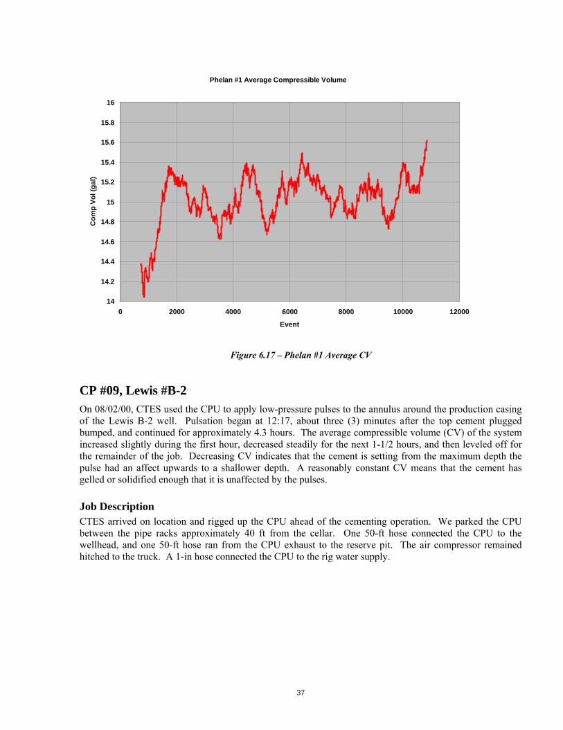
CP #08, Phelan #1 On 07/29/00, CTES used the CPU to apply low-pressure pulses to the annulus around the intermediate casing of the Phelan #1 well. This was our first directional well attempted to date. Pulsation began about three (3) minutes after the top cement plugged bumped and continued for approximately four (4) hours. The average compressible volume (CV) of the system (the volume of fluid in each pulse) increased from about 14 gal to about 15.4 gal during the first 35 minutes. For the remainder of the job, the average CV was 15±0.4 gal. The initial increase in average CV indicates that the pulsations progressively overcame the static gel strengths of the mud and cement. The average CV should decrease later in the job as the cement’s static gel strength increases, but this did not happen. Thus, either the cement’s response to the pulsations was masked from the CPU’s instrumentation or the cement had not begun to set during the CP job.

Job Description CTES arrived on location and rigged up the CPU ahead of the cementing operation. We parked the CPU between the rig and the pipe racks approximately 30 ft from the cellar. One 50-ft hose connected the CPU to the wellhead, and one 50-ft hose ran from the CPU exhaust to the reserve pit. We left the air compressor hitched to the truck. A 1-in hose connected the CPU to the rig water supply. After rigging up the CPU and completing all of the external connections we confirmed that the CPU was ready for normal operations by applying a few pulses against the closed wellhead valve. We placed the CPU in standby mode pending completion of the cement job. The rig crew opened the wellhead valve before BJ started pumping spacer. By prior arrangement with the host supervisor and tool pusher, the rig crew closed the annular BOP shortly after the top cement plug bumped. We commenced pulsing the annulus with 105-110 psi water at 14:30. The CPU operated normally throughout the job. The CPU steadily supplied about 33.3 gal of water per hour to the well during the job. The CPU data indicated that the compressibility of the

6

7

8

9

10

11

12

13

14

2000 4000 6000 8000 10000 12000 14000

Event

Co

mp

Vo

l (g

al)

Comp Vol

Avg CV

Linear Fit, CV

Linear Fit, Avg CV

35

wellbore was not changing, so we stopped pulsation after four (4) hours. We rigged down the CPU and left the location by 19:15.

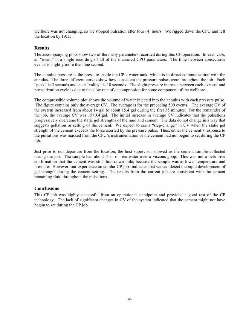
Results The accompanying plots show two of the many parameters recorded during this CP operation. In each case, an “event” is a single recording of all of the measured CPU parameters. The time between consecutive events is slightly more than one second. The annulus pressure is the pressure inside the CPU water tank, which is in direct communication with the annulus. The three different curves show how consistent the pressure pulses were throughout the job. Each “peak” is 5 seconds and each “valley” is 10 seconds. The slight pressure increase between each exhaust and pressurization cycle is due to the slow rate of decompression for some component of the wellbore. The compressible volume plot shows the volume of water injected into the annulus with each pressure pulse. The figure contains only the average CV. The average is for the preceding 500 events. The average CV of the system increased from about 14 gal to about 15.4 gal during the first 35 minutes. For the remainder of the job, the average CV was 15±0.4 gal. The initial increase in average CV indicates that the pulsations progressively overcame the static gel strengths of the mud and cement. The data do not change in a way that suggests gellation or setting of the cement. We expect to see a “step-change” in CV when the static gel strength of the cement exceeds the force exerted by the pressure pulse. Thus, either the cement’s response to the pulsations was masked from the CPU’s instrumentation or the cement had not begun to set during the CP job. Just prior to our departure from the location, the host supervisor showed us the cement sample collected during the job. The sample had about ½ in of free water over a viscous goop. This was not a definitive confirmation that the cement was still fluid down hole, because the sample was at lower temperature and pressure. However, our experience on similar CP jobs indicates that we can detect the rapid development of gel strength during the cement setting. The results from the current job are consistent with the cement remaining fluid throughout the pulsations.

Conclusions This CP job was highly successful from an operational standpoint and provided a good test of the CP technology. The lack of significant changes in CV of the system indicated that the cement might not have begun to set during the CP job.

36

Figure 6.16 – Phelan #1 Annulus Pressures

Phelan #1 Annulus Pressure

0

20

40

60

80

100

120

0 10 20 30 40 50 60 70

Event

An

nu

lus

Pre

ssu

re (

psi

)

14:45

16:42

18:13

Start Time

37

Figure 6.17 – Phelan #1 Average CV

CP #09, Lewis #B-2 On 08/02/00, CTES used the CPU to apply low-pressure pulses to the annulus around the production casing of the Lewis B-2 well. Pulsation began at 12:17, about three (3) minutes after the top cement plugged bumped, and continued for approximately 4.3 hours. The average compressible volume (CV) of the system increased slightly during the first hour, decreased steadily for the next 1-1/2 hours, and then leveled off for the remainder of the job. Decreasing CV indicates that the cement is setting from the maximum depth the pulse had an affect upwards to a shallower depth. A reasonably constant CV means that the cement has gelled or solidified enough that it is unaffected by the pulses.

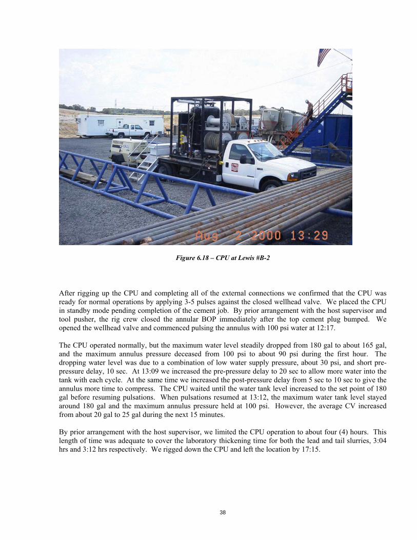
Job Description CTES arrived on location and rigged up the CPU ahead of the cementing operation. We parked the CPU between the pipe racks approximately 40 ft from the cellar. One 50-ft hose connected the CPU to the wellhead, and one 50-ft hose ran from the CPU exhaust to the reserve pit. The air compressor remained hitched to the truck. A 1-in hose connected the CPU to the rig water supply.

Phelan #1 Average Compressible Volume

14

14.2

14.4

14.6

14.8

15

15.2

15.4

15.6

15.8

16

0 2000 4000 6000 8000 10000 12000

Event

Co

mp

Vo

l (g

al)

38

Figure 6.18 – CPU at Lewis #B-2

After rigging up the CPU and completing all of the external connections we confirmed that the CPU was ready for normal operations by applying 3-5 pulses against the closed wellhead valve. We placed the CPU in standby mode pending completion of the cement job. By prior arrangement with the host supervisor and tool pusher, the rig crew closed the annular BOP immediately after the top cement plug bumped. We opened the wellhead valve and commenced pulsing the annulus with 100 psi water at 12:17. The CPU operated normally, but the maximum water level steadily dropped from 180 gal to about 165 gal, and the maximum annulus pressure deceased from 100 psi to about 90 psi during the first hour. The dropping water level was due to a combination of low water supply pressure, about 30 psi, and short pre-pressure delay, 10 sec. At 13:09 we increased the pre-pressure delay to 20 sec to allow more water into the tank with each cycle. At the same time we increased the post-pressure delay from 5 sec to 10 sec to give the annulus more time to compress. The CPU waited until the water tank level increased to the set point of 180 gal before resuming pulsations. When pulsations resumed at 13:12, the maximum water tank level stayed around 180 gal and the maximum annulus pressure held at 100 psi. However, the average CV increased from about 20 gal to 25 gal during the next 15 minutes. By prior arrangement with the host supervisor, we limited the CPU operation to about four (4) hours. This length of time was adequate to cover the laboratory thickening time for both the lead and tail slurries, 3:04 hrs and 3:12 hrs respectively. We rigged down the CPU and left the location by 17:15.

39

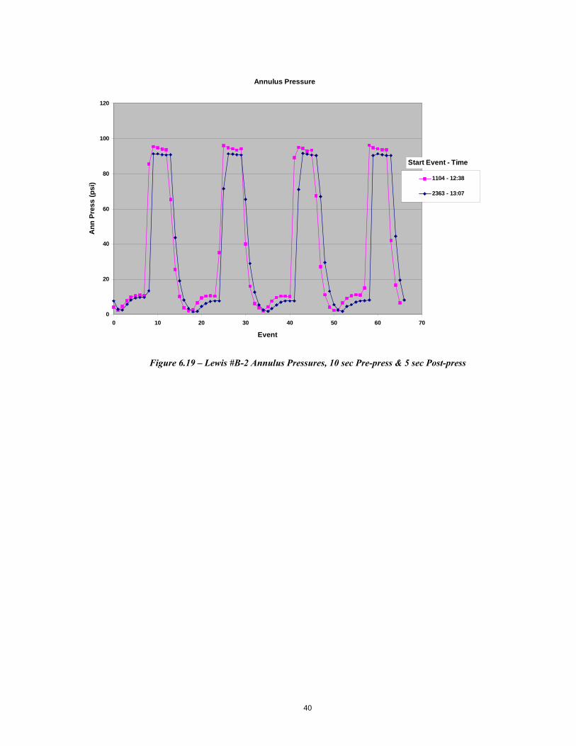
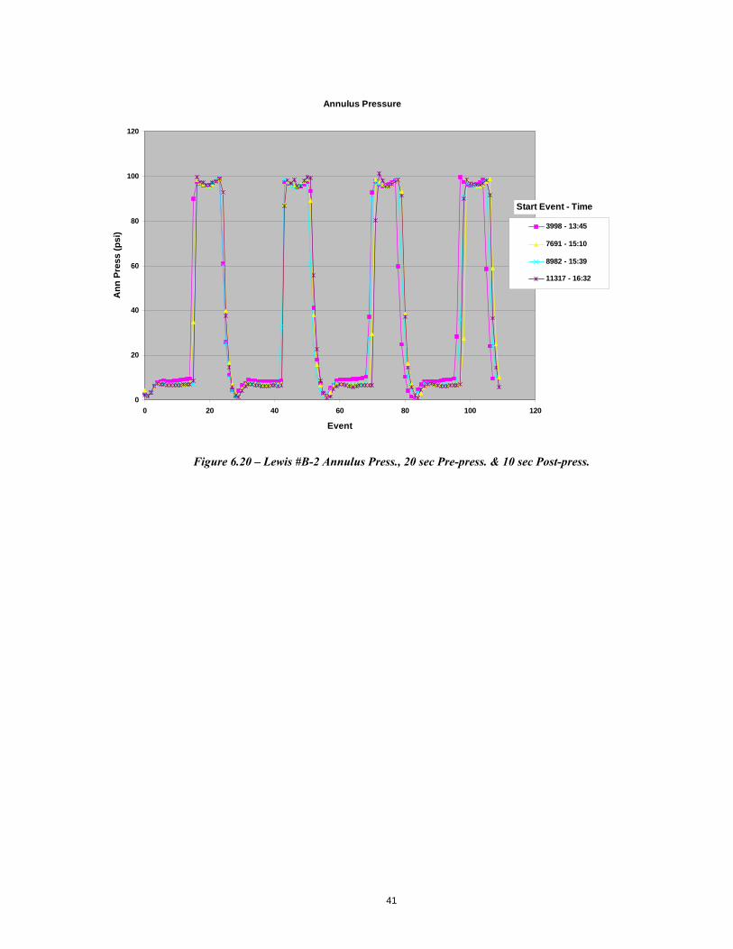
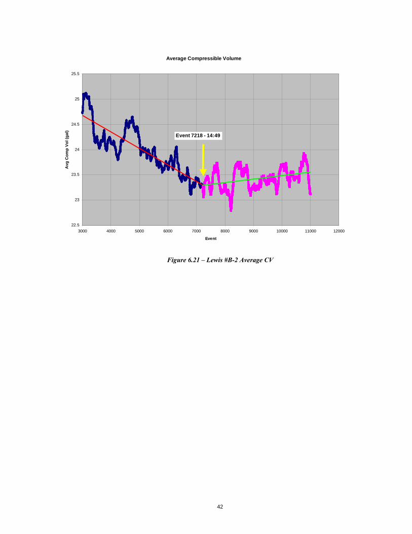
Results The first plot below shows the pressure inside the CPU water tank, which is in direct communication with the annulus, during the first hour of operation. The pre-pressure delay was 10 sec (valley) and the post-pressure delay was 5 sec (peak). An event is one recording of all measured parameters. The x-axis is the number of the event relative to the start of the pulsation cycle. The event shown in the plot legend is relative to the start of the job. Note the decrease in maximum pressure and corresponding increase in cycle time for the 30-min period represented by the plot. These changes were due to the decreasing water tank level. The second plot below shows selected annulus pressures later in the job when the pre-pressure delay was 20 sec (valley) and the post-pressure delay was 10 sec (peak). The maximum water tank level had stabilized by 13:35. Note the consistency of the data over a 3-hr period. The average compressible volume plot shows the average volume of water injected into the annulus with each pressure pulse. Each value plotted is the average of the preceding 500 events. The x-axis is the event relative to the start of the job, and the plot starts after the CPU operation had stabilized from resetting the pressure delays. The steady decrease in CV for about 1-1/2 hours indicates that the cement was gelling or setting, starting at the maximum depth the pulse could penetrate and progressing upwards. At approximately event 7218 (14:49), the average CV leveled off. This indicates that the volume of cement that had been affected by the pressure pulses was now gelled or set enough that the pulses were ineffective. The laboratory thickening time for both the lead and tail slurries was approximately 3:08 hours. This corresponds roughly to 14:38 (event 6292), assuming the clock started when pumping the cement commenced.

Conclusions This CP job was reasonably successful from an operational standpoint and provided valuable data for developing a better understanding of how the wellbore and cement respond to low-pressure pulses. The abrupt change in CV of the system at approximately the expected thickening time of the cement is strong evidence the CV data can be useful as a diagnostic tool.

40

Figure 6.19 – Lewis #B-2 Annulus Pressures, 10 sec Pre-press & 5 sec Post-press

Annulus Pressure

0

20

40

60

80

100

120

0 10 20 30 40 50 60 70

Event

An

n P

ress

(p

si)

1104 - 12:38

2363 - 13:07

Start Event - Time

41

Figure 6.20 – Lewis #B-2 Annulus Press., 20 sec Pre-press. & 10 sec Post-press.

Annulus Pressure

0

20

40

60

80

100

120

0 20 40 60 80 100 120

Event

An

n P

ress

(p

si)

3998 - 13:45

7691 - 15:10

8982 - 15:39

11317 - 16:32

Start Event - Time

42

Figure 6.21 – Lewis #B-2 Average CV

Average Compressible Volume

22.5

23

23.5

24

24.5

25

25.5

3000 4000 5000 6000 7000 8000 9000 10000 11000 12000

Event

Avg

Co

mp

Vo

l (g

al)

Event 7218 - 14:49

43

TASK 7 – CP TESTS WITH DOWNHOLE MEASUREMENTS

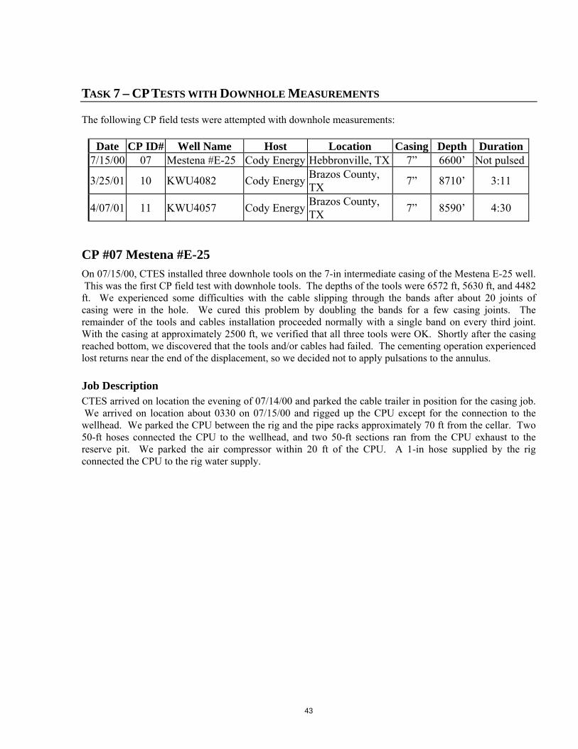
The following CP field tests were attempted with downhole measurements:

Date CP ID# Well Name Host Location Casing Depth Duration7/15/00 07 Mestena #E-25 Cody Energy Hebbronville, TX 7” 6600’ Not pulsed

3/25/01 10 KWU4082 Cody EnergyBrazos County, TX

7” 8710’ 3:11

4/07/01 11 KWU4057 Cody EnergyBrazos County, TX

7” 8590’ 4:30

CP #07 Mestena #E-25 On 07/15/00, CTES installed three downhole tools on the 7-in intermediate casing of the Mestena E-25 well. This was the first CP field test with downhole tools. The depths of the tools were 6572 ft, 5630 ft, and 4482 ft. We experienced some difficulties with the cable slipping through the bands after about 20 joints of casing were in the hole. We cured this problem by doubling the bands for a few casing joints. The remainder of the tools and cables installation proceeded normally with a single band on every third joint. With the casing at approximately 2500 ft, we verified that all three tools were OK. Shortly after the casing reached bottom, we discovered that the tools and/or cables had failed. The cementing operation experienced lost returns near the end of the displacement, so we decided not to apply pulsations to the annulus.

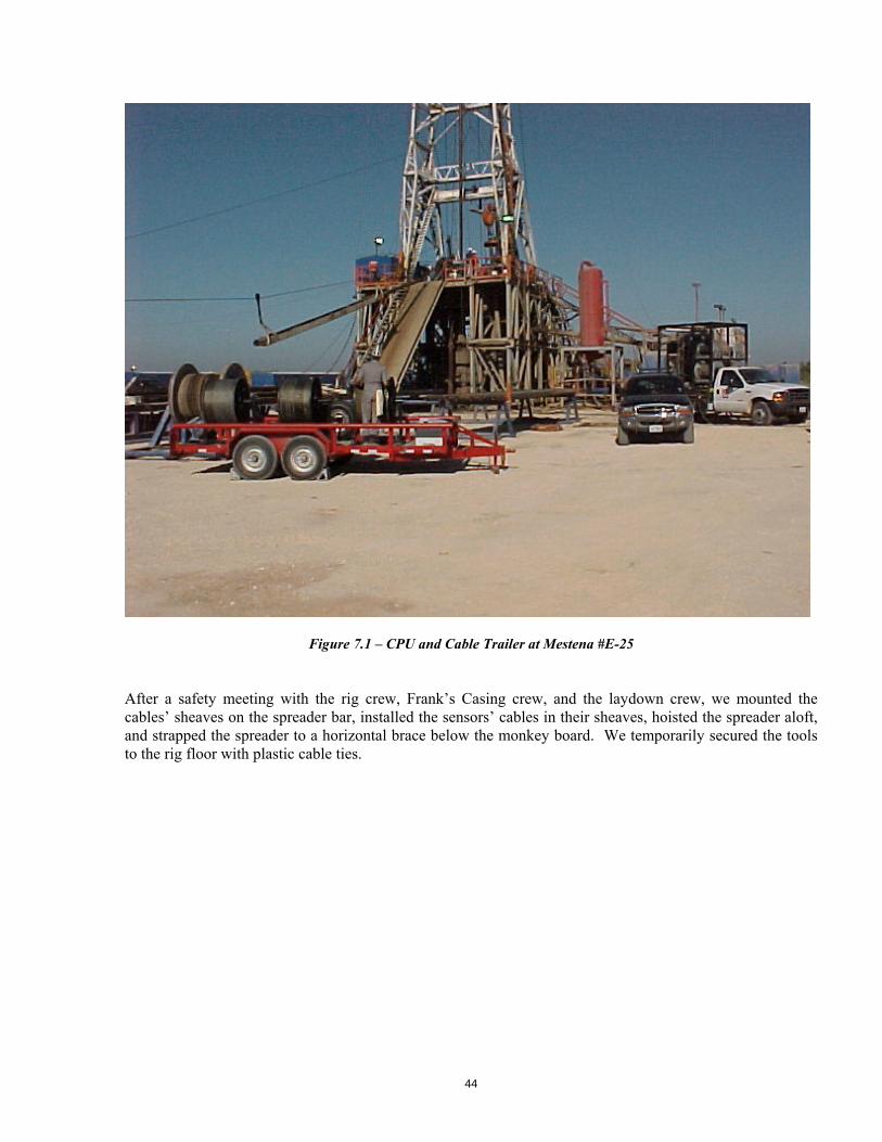
Job Description CTES arrived on location the evening of 07/14/00 and parked the cable trailer in position for the casing job. We arrived on location about 0330 on 07/15/00 and rigged up the CPU except for the connection to the wellhead. We parked the CPU between the rig and the pipe racks approximately 70 ft from the cellar. Two 50-ft hoses connected the CPU to the wellhead, and two 50-ft sections ran from the CPU exhaust to the reserve pit. We parked the air compressor within 20 ft of the CPU. A 1-in hose supplied by the rig connected the CPU to the rig water supply.

44

Figure 7.1 – CPU and Cable Trailer at Mestena #E-25

After a safety meeting with the rig crew, Frank’s Casing crew, and the laydown crew, we mounted the cables’ sheaves on the spreader bar, installed the sensors’ cables in their sheaves, hoisted the spreader aloft, and strapped the spreader to a horizontal brace below the monkey board. We temporarily secured the tools to the rig floor with plastic cable ties.

45

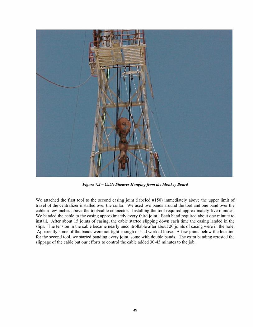
Figure 7.2 – Cable Sheaves Hanging from the Monkey Board

We attached the first tool to the second casing joint (labeled #150) immediately above the upper limit of travel of the centralizer installed over the collar. We used two bands around the tool and one band over the cable a few inches above the tool/cable connector. Installing the tool required approximately five minutes. We banded the cable to the casing approximately every third joint. Each band required about one minute to install. After about 15 joints of casing, the cable started slipping down each time the casing landed in the slips. The tension in the cable became nearly uncontrollable after about 20 joints of casing were in the hole. Apparently some of the bands were not tight enough or had worked loose. A few joints below the location for the second tool, we started banding every joint, some with double bands. The extra banding arrested the slippage of the cable but our efforts to control the cable added 30-45 minutes to the job.

46

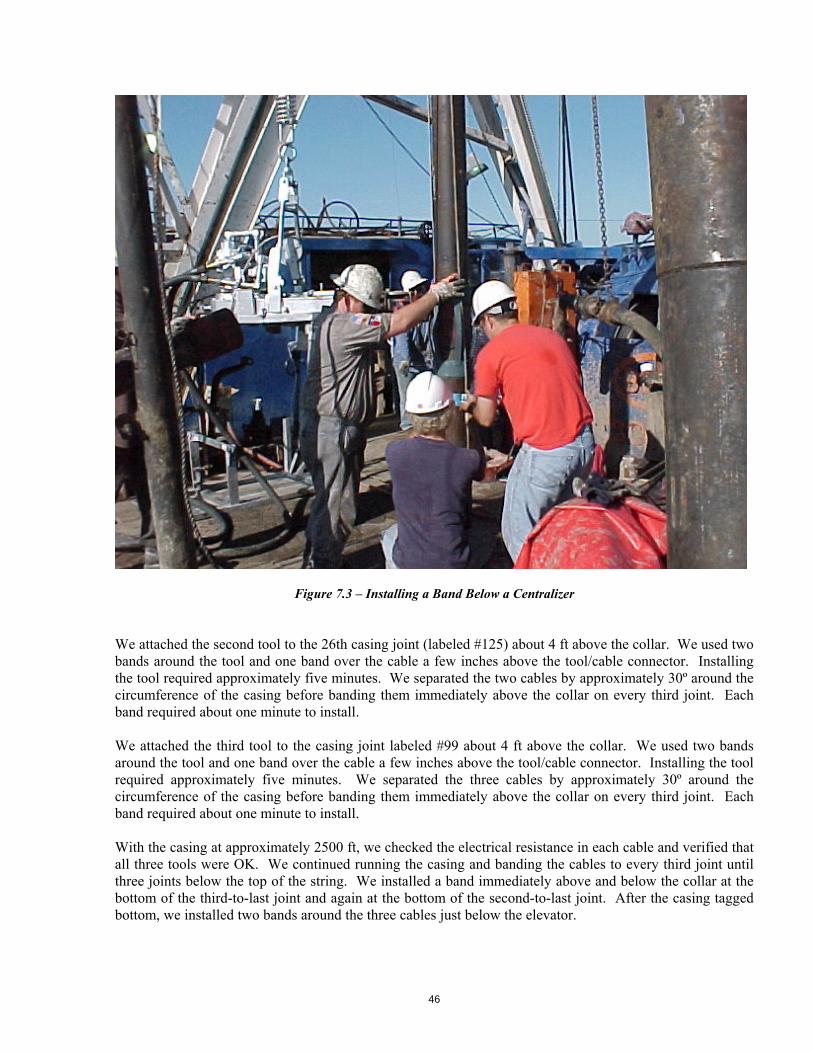
Figure 7.3 – Installing a Band Below a Centralizer

We attached the second tool to the 26th casing joint (labeled #125) about 4 ft above the collar. We used two bands around the tool and one band over the cable a few inches above the tool/cable connector. Installing the tool required approximately five minutes. We separated the two cables by approximately 30º around the circumference of the casing before banding them immediately above the collar on every third joint. Each band required about one minute to install. We attached the third tool to the casing joint labeled #99 about 4 ft above the collar. We used two bands around the tool and one band over the cable a few inches above the tool/cable connector. Installing the tool required approximately five minutes. We separated the three cables by approximately 30º around the circumference of the casing before banding them immediately above the collar on every third joint. Each band required about one minute to install. With the casing at approximately 2500 ft, we checked the electrical resistance in each cable and verified that all three tools were OK. We continued running the casing and banding the cables to every third joint until three joints below the top of the string. We installed a band immediately above and below the collar at the bottom of the third-to-last joint and again at the bottom of the second-to-last joint. After the casing tagged bottom, we installed two bands around the three cables just below the elevator.

47

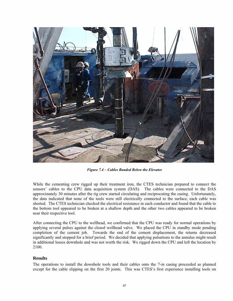
Figure 7.4 – Cables Banded Below the Elevator

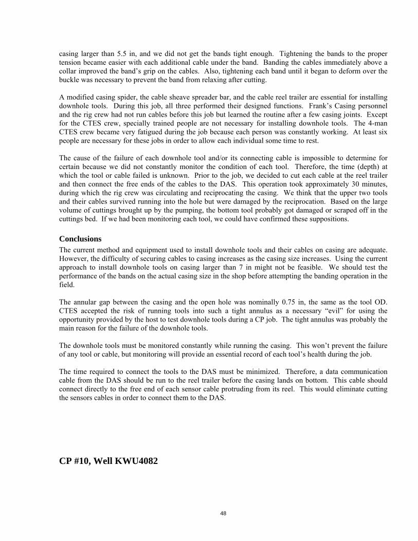
While the cementing crew rigged up their treatment iron, the CTES technician prepared to connect the sensors’ cables to the CPU data acquisition system (DAS). The cables were connected to the DAS approximately 30 minutes after the rig crew started circulating and reciprocating the casing. Unfortunately, the data indicated that none of the tools were still electrically connected to the surface; each cable was shorted. The CTES technician checked the electrical resistance in each conductor and found that the cable to the bottom tool appeared to be broken at a shallow depth and the other two cables appeared to be broken near their respective tool. After connecting the CPU to the wellhead, we confirmed that the CPU was ready for normal operations by applying several pulses against the closed wellhead valve. We placed the CPU in standby mode pending completion of the cement job. Towards the end of the cement displacement, the returns decreased significantly and stopped for a brief period. We decided that applying pulsations to the annulus might result in additional losses downhole and was not worth the risk. We rigged down the CPU and left the location by 2100.

Results The operations to install the downhole tools and their cables onto the 7-in casing proceeded as planned except for the cable slipping on the first 20 joints. This was CTES’s first experience installing tools on

48

casing larger than 5.5 in, and we did not get the bands tight enough. Tightening the bands to the proper tension became easier with each additional cable under the band. Banding the cables immediately above a collar improved the band’s grip on the cables. Also, tightening each band until it began to deform over the buckle was necessary to prevent the band from relaxing after cutting. A modified casing spider, the cable sheave spreader bar, and the cable reel trailer are essential for installing downhole tools. During this job, all three performed their designed functions. Frank’s Casing personnel and the rig crew had not run cables before this job but learned the routine after a few casing joints. Except for the CTES crew, specially trained people are not necessary for installing downhole tools. The 4-man CTES crew became very fatigued during the job because each person was constantly working. At least six people are necessary for these jobs in order to allow each individual some time to rest. The cause of the failure of each downhole tool and/or its connecting cable is impossible to determine for certain because we did not constantly monitor the condition of each tool. Therefore, the time (depth) at which the tool or cable failed is unknown. Prior to the job, we decided to cut each cable at the reel trailer and then connect the free ends of the cables to the DAS. This operation took approximately 30 minutes, during which the rig crew was circulating and reciprocating the casing. We think that the upper two tools and their cables survived running into the hole but were damaged by the reciprocation. Based on the large volume of cuttings brought up by the pumping, the bottom tool probably got damaged or scraped off in the cuttings bed. If we had been monitoring each tool, we could have confirmed these suppositions.

Conclusions The current method and equipment used to install downhole tools and their cables on casing are adequate. However, the difficulty of securing cables to casing increases as the casing size increases. Using the current approach to install downhole tools on casing larger than 7 in might not be feasible. We should test the performance of the bands on the actual casing size in the shop before attempting the banding operation in the field. The annular gap between the casing and the open hole was nominally 0.75 in, the same as the tool OD. CTES accepted the risk of running tools into such a tight annulus as a necessary “evil” for using the opportunity provided by the host to test downhole tools during a CP job. The tight annulus was probably the main reason for the failure of the downhole tools. The downhole tools must be monitored constantly while running the casing. This won’t prevent the failure of any tool or cable, but monitoring will provide an essential record of each tool’s health during the job. The time required to connect the tools to the DAS must be minimized. Therefore, a data communication cable from the DAS should be run to the reel trailer before the casing lands on bottom. This cable should connect directly to the free end of each sensor cable protruding from its reel. This would eliminate cutting the sensors cables in order to connect them to the DAS.

CP #10, Well KWU4082

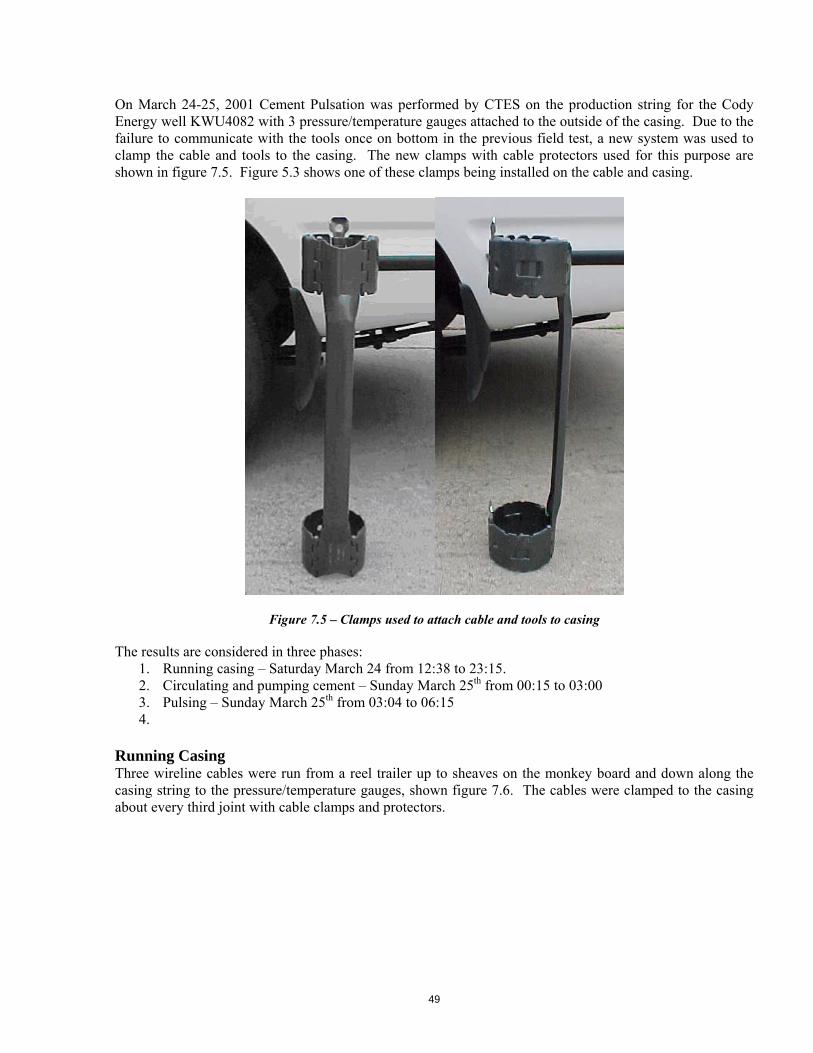
49

On March 24-25, 2001 Cement Pulsation was performed by CTES on the production string for the Cody Energy well KWU4082 with 3 pressure/temperature gauges attached to the outside of the casing. Due to the failure to communicate with the tools once on bottom in the previous field test, a new system was used to clamp the cable and tools to the casing. The new clamps with cable protectors used for this purpose are shown in figure 7.5. Figure 5.3 shows one of these clamps being installed on the cable and casing.

Figure 7.5 – Clamps used to attach cable and tools to casing

The results are considered in three phases: 1. Running casing – Saturday March 24 from 12:38 to 23:15. 2. Circulating and pumping cement – Sunday March 25th from 00:15 to 03:00 3. Pulsing – Sunday March 25th from 03:04 to 06:15 4.

Running Casing Three wireline cables were run from a reel trailer up to sheaves on the monkey board and down along the casing string to the pressure/temperature gauges, shown figure 7.6. The cables were clamped to the casing about every third joint with cable clamps and protectors.

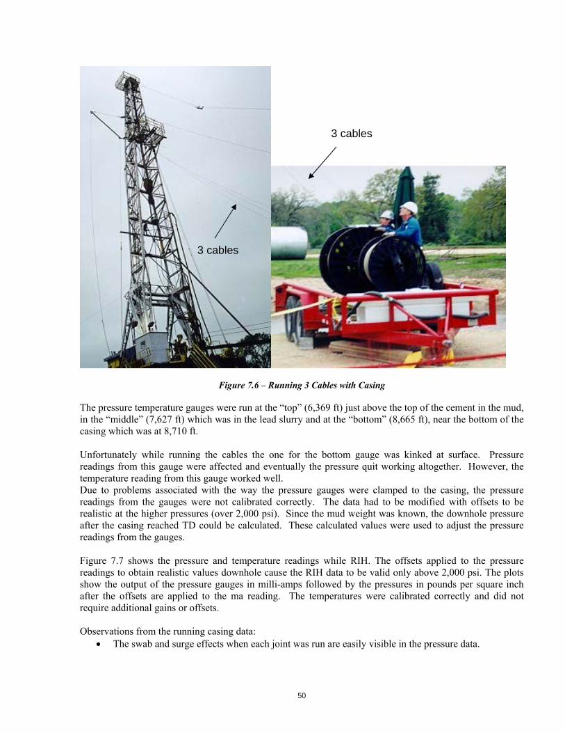
50

Figure 7.6 – Running 3 Cables with Casing

The pressure temperature gauges were run at the “top” (6,369 ft) just above the top of the cement in the mud, in the “middle” (7,627 ft) which was in the lead slurry and at the “bottom” (8,665 ft), near the bottom of the casing which was at 8,710 ft. Unfortunately while running the cables the one for the bottom gauge was kinked at surface. Pressure readings from this gauge were affected and eventually the pressure quit working altogether. However, the temperature reading from this gauge worked well. Due to problems associated with the way the pressure gauges were clamped to the casing, the pressure readings from the gauges were not calibrated correctly. The data had to be modified with offsets to be realistic at the higher pressures (over 2,000 psi). Since the mud weight was known, the downhole pressure after the casing reached TD could be calculated. These calculated values were used to adjust the pressure readings from the gauges. Figure 7.7 shows the pressure and temperature readings while RIH. The offsets applied to the pressure readings to obtain realistic values downhole cause the RIH data to be valid only above 2,000 psi. The plots show the output of the pressure gauges in milli-amps followed by the pressures in pounds per square inch after the offsets are applied to the ma reading. The temperatures were calibrated correctly and did not require additional gains or offsets. Observations from the running casing data:

The swab and surge effects when each joint was run are easily visible in the pressure data.

3 cables

3 cables

51

They stopped running casing at several points to fill the casing with mud. As would be expected, the pressure in the annulus was constant during these stops. It is interesting that during these stops the temperatures decreased slightly due to the casing and mud cooling down the annulus.

During one stop at 17:45 mud was pumped through the casing to verify that circulation could be established through the float shoe. This is seen by the dip in temperature primarily at the bottom and middle gauges.

The casing reached bottom at 23:17. The cables were banded high enough to allow for the travel when the casing was reciprocated. Circulating and Cementing Figure 7.8 shows the data for this stage. Mud was circulated until 1:22 am at which time Schlumberger began rigging up for pumping cement. During this time the temperature at all 3 gauges decreased significantly as the mud cooled the annulus. There is an interesting stretch of time from 1:22 when circulation was stopped until 1:40 when Schlumberger began recording surface data. During this time the temperature continued to decrease as would be expected. However, the pressure at both gauges also decreased very linearly by about 225 psi. This pressure did not seem to recover. Currently we cannot explain this pressure drop. At 1:43 Schlumberger circulated very briefly. The resulting pressure spike can be seen at surface and at the downhole gauges. They pressure tested at 1:52 and began pumping cement. The surface pressure decreased as the heavier cement was pumped and then increased as the cement circulated up the annulus until the plug was bumped at 3:00. Pulsing Figure 7.9 shows the data for this stage. About 4 minutes after the plug was bumped the cement pulsation (CP) system began applying 100 psi pulses to the casing annulus at surface. The data gathered during the pulsing is shown in the attached “Pulsation Data” graphs. Observations from this data:

As can be seen from the “One Minute of Pulsing” graph, it took about 2 seconds to apply the 100 psi of pressure. This pressure was held for 10 seconds and then was released. There was then a 10 second delay before the next pulse was applied.

About 2 seconds after the pressure was applied at surface, the pressure began to increase at the top gauge. A short time later the pressure began to increase at the middle gauge. Data was being acquired at 1-second intervals which is not fast enough to accurately measure the speed of sound in the mud.

During the initial pulsation the amplitude of the pulse at the top gauge was about 90 psi. The amplitude of the pulse at the middle gauge starts out at about 64 psi.

As the cement set, the amplitude of the pressure at the middle gauge (which was near the bottom of the lead slurry) decreased gradually to zero amplitude over 3 hours. During this time the hydrostatic pressure remained fairly constant at 3,990 psi, decreasing only about 40 psi at the end of the cement setting.

The pulsation did not seem to have any affect on the temperatures, which rose steadily towards the surrounding ambient temperature. There was no significant increase in temperature seen due to the exothermic reaction of the cement setting.

If the entire annulus was full of cement, we would expect the compressible volume to decrease to zero as the cement sets. However, for this well the cement only filled the bottom 25% of the column.

There was one point at which the compressible volume decreased suddenly from about 14 gallons to about 11 gallons. This corresponded to an abrupt inflow of a couple of gallons of water to the

52

system. Air trapped in the system must have suddenly escaped through the annular preventer, decreasing the compressibility of the system. After this sudden change, some water was continually added to the system at a rate of about 5 gallons per hour. This was probably due to observed leakage around the cables through the annular with each pulse.

Summary It is clear that pressure pulses did reach the top and middle gauges. The pressure attenuation in the mud was 1.6 psi per 1,000 ft. The attenuation in the lead slurry was 20.7 psi per 1,000 ft. However, due to the calibration problems discussed previously we cannot be certain about these attenuations. The pressure pulses did keep the hydrostatic pressure from decreasing significantly at the middle gauge.

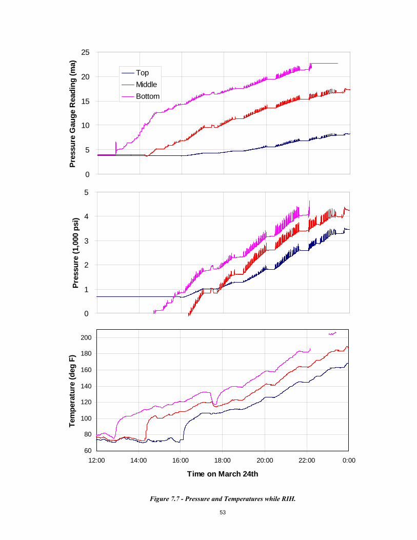
53

Figure 7.7 - Pressure and Temperatures while RIH.

0

5

10

15

20

25

Pre

ssu

re G

aug

e R

ead

ing

(m

a)Top

Middle

Bottom

0

1

2

3

4

5

Pre

ssu

re (

1,00

0 p

si)

60

80

100

120

140

160

180

200

12:00 14:00 16:00 18:00 20:00 22:00 0:00

Time on March 24th

Tem

per

atu

re (

deg

F)

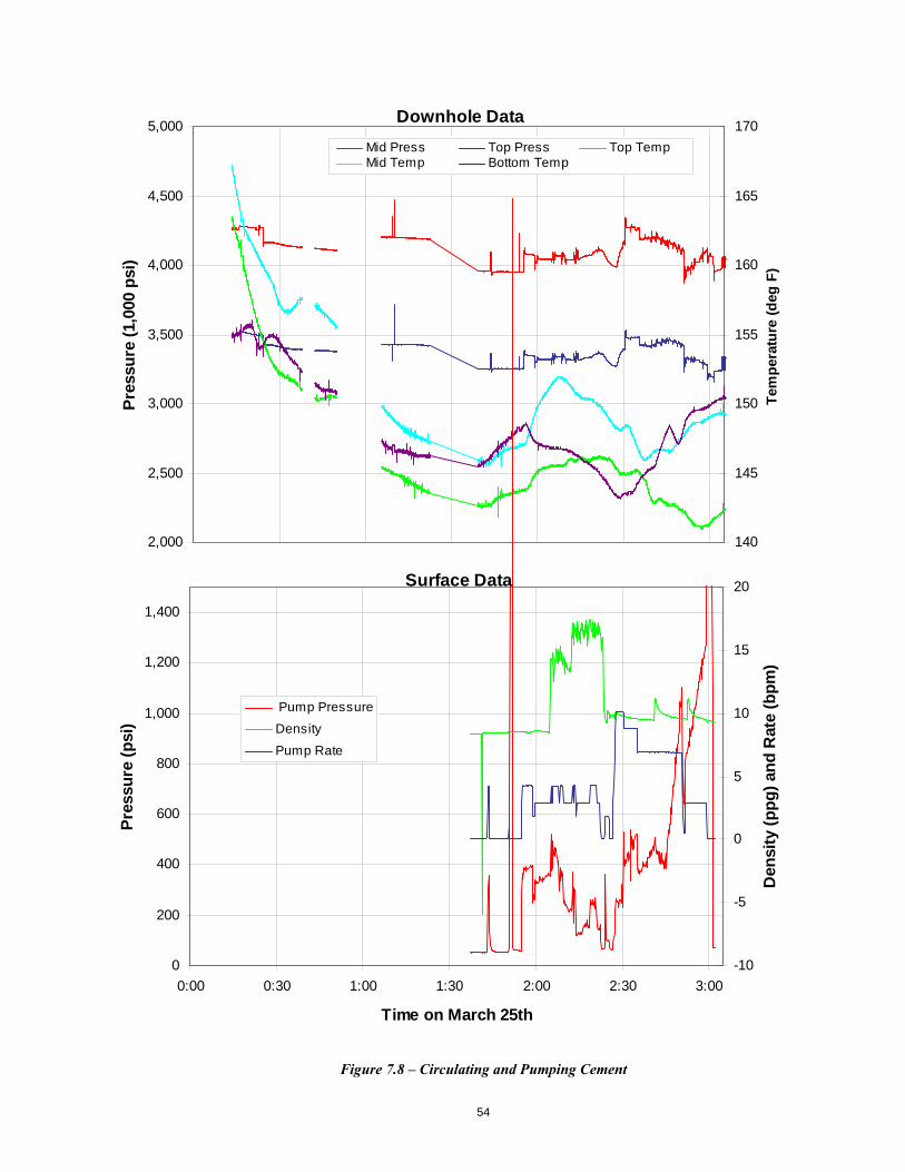
54

Figure 7.8 – Circulating and Pumping Cement

Downhole Data

2,000

2,500

3,000

3,500

4,000

4,500

5,000P

ress

ure

(1,

000

psi

)

140

145

150

155

160

165

170

Tem

per

atu

re (

deg

F)

Mid Press Top Press Top TempMid Temp Bottom Temp

Surface Data

0

200

400

600

800

1,000

1,200

1,400

0:00 0:30 1:00 1:30 2:00 2:30 3:00

Time on March 25th

Pre

ssu

re (

psi

)

-10

-5

0

5

10

15

20

Den

sity

(p

pg

) an

d R

ate

(bp

m)

Pump Pressure

Density

Pump Rate

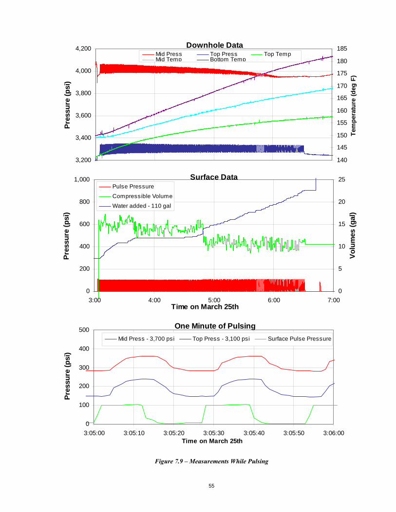
55

Figure 7.9 – Measurements While Pulsing

Downhole Data

3,200

3,400

3,600

3,800

4,000

4,200

Pre

ssu

re (

psi

)

140

145

150

155

160

165

170

175

180

185

Tem

per

atu

re (

deg

F)

Mid Press Top Press Top TempMid Temp Bottom Temp

Surface Data

0

200

400

600

800

1,000

3:00 4:00 5:00 6:00 7:00Time on March 25th

Pre

ssu

re (

psi

)

0

5

10

15

20

25

Vo

lum

es (

gal

)

Pulse Pressure

Compressible Volume

Water added - 110 gal

One Minute of Pulsing

0

100

200

300

400

500

3:05:00 3:05:10 3:05:20 3:05:30 3:05:40 3:05:50 3:06:00Time on March 25th

Pre

ssu

re (

psi

)

Mid Press - 3,700 psi Top Press - 3,100 psi Surface Pulse Pressure

56

CP # 11, KWU4057

On April 6-7, 2001 Cement Pulsation was performed on the production string for the Cody Energy well KWU4057 with 3 pressure/temperature gauges attached to the outside of the casing. The results are considered in three phases:

5. Running casing – from 16:25 PM on April 6th till 00:45 AM on April 7th 6. Circulating and pumping cement – from 1:00 AM till 3:55 AM on April 7th 7. Pulsing – from 4:01 AM till 8:30 AM on April 7th

Running Casing The pressure temperature gauges were run at the “top” (6,986 ft) at the top of the lead slurry, in the “middle” (7,800 ft) which was in the top of the tail slurry and at the “bottom” (8,544 ft), near the bottom of the casing which was at 8,590 ft. Due to problems associated with the way the pressure gauges were clamped to the casing, the pressure readings from the gauges were not calibrated correctly. Calibration curves were developed after the job to correct for these problems. Since the mud weight was known, the downhole pressure at various depths could be calculated. These calculated values were used to adjust the pressure readings from the gauges. The plots in Figure 7.10 show the pressure and temperatures while RIH. Observations from the running casing data:

The swab and surge effects when each joint was run are easily visible in the pressure data. They stopped running casing at several points to fill the casing with mud. As would be expected,

the pressure in the annulus was fairly constant during these stops. During one stop at 20:23 mud was pumped through the casing to verify that circulation could be

established through the float shoe. A slight upward blip is seen in the pressure when the pumping started. A dip is seen in the temperature at the bottom gauge as cooler fluid from above was circulated through the float shoe.

The last few minutes of data show an increase in pressure as they started circulating mud after the casing was on bottom. This caused a rapid decrease in the temperature at the bottom gauge as cooler mud was circulated through the float shoe. The temperature from the middle gauge actually increases slightly as warmer mud from below moves up the annulus.

The temperature of the bottom gauge seems too close to the temperature of the middle gauge. At this point it is not clear if this is correct or an error in the measurement. Unlike the pressure calibration, no adjustments have been made to the temperature calibration for any of the gauges.

The casing reached bottom at 00:45 AM. The cables were banded high enough to allow for the travel when the casing was reciprocated. Circulating and Cementing Figure 7.11 shows the data from the circulating and cementing operation. Mud was circulated until 2:19 am at which time Schlumberger began rigging up for pumping cement. They pressure tested at 2:51 and started pumping at 2:53. They must have circulated very briefly at 2:48, though they didn’t record any surface data at that time. From the data it appears that they finished pumping cement at 3:20 and began displacing with water at 3:26. The cement appears to have reached the shoe at 3:42, the bottom pressure gauge at 3:43, and the middle pressure gauge at 3:46. The pump rate was reduced at 3:52 from 7 bpm to 2.5 bpm and the plug was bumped at 3:55.

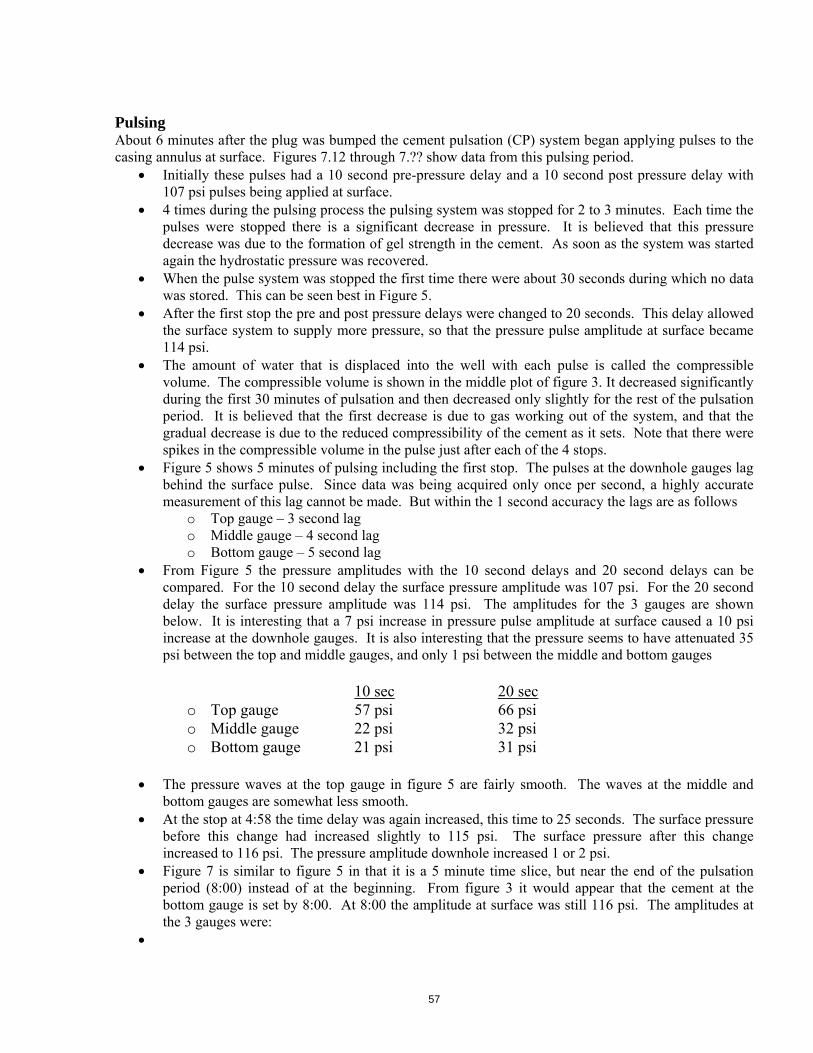
57

Pulsing About 6 minutes after the plug was bumped the cement pulsation (CP) system began applying pulses to the casing annulus at surface. Figures 7.12 through 7.?? show data from this pulsing period.

Initially these pulses had a 10 second pre-pressure delay and a 10 second post pressure delay with 107 psi pulses being applied at surface.

4 times during the pulsing process the pulsing system was stopped for 2 to 3 minutes. Each time the pulses were stopped there is a significant decrease in pressure. It is believed that this pressure decrease was due to the formation of gel strength in the cement. As soon as the system was started again the hydrostatic pressure was recovered.

When the pulse system was stopped the first time there were about 30 seconds during which no data was stored. This can be seen best in Figure 5.

After the first stop the pre and post pressure delays were changed to 20 seconds. This delay allowed the surface system to supply more pressure, so that the pressure pulse amplitude at surface became 114 psi.

The amount of water that is displaced into the well with each pulse is called the compressible volume. The compressible volume is shown in the middle plot of figure 3. It decreased significantly during the first 30 minutes of pulsation and then decreased only slightly for the rest of the pulsation period. It is believed that the first decrease is due to gas working out of the system, and that the gradual decrease is due to the reduced compressibility of the cement as it sets. Note that there were spikes in the compressible volume in the pulse just after each of the 4 stops.

Figure 5 shows 5 minutes of pulsing including the first stop. The pulses at the downhole gauges lag behind the surface pulse. Since data was being acquired only once per second, a highly accurate measurement of this lag cannot be made. But within the 1 second accuracy the lags are as follows

o Top gauge – 3 second lag o Middle gauge – 4 second lag o Bottom gauge – 5 second lag

From Figure 5 the pressure amplitudes with the 10 second delays and 20 second delays can be compared. For the 10 second delay the surface pressure amplitude was 107 psi. For the 20 second delay the surface pressure amplitude was 114 psi. The amplitudes for the 3 gauges are shown below. It is interesting that a 7 psi increase in pressure pulse amplitude at surface caused a 10 psi increase at the downhole gauges. It is also interesting that the pressure seems to have attenuated 35 psi between the top and middle gauges, and only 1 psi between the middle and bottom gauges

10 sec 20 sec

o Top gauge 57 psi 66 psi o Middle gauge 22 psi 32 psi o Bottom gauge 21 psi 31 psi

The pressure waves at the top gauge in figure 5 are fairly smooth. The waves at the middle and

bottom gauges are somewhat less smooth. At the stop at 4:58 the time delay was again increased, this time to 25 seconds. The surface pressure

before this change had increased slightly to 115 psi. The surface pressure after this change increased to 116 psi. The pressure amplitude downhole increased 1 or 2 psi.

Figure 7 is similar to figure 5 in that it is a 5 minute time slice, but near the end of the pulsation period (8:00) instead of at the beginning. From figure 3 it would appear that the cement at the bottom gauge is set by 8:00. At 8:00 the amplitude at surface was still 116 psi. The amplitudes at the 3 gauges were:

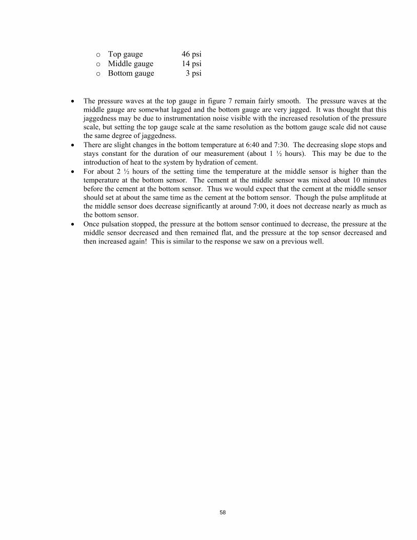
58

o Top gauge 46 psi o Middle gauge 14 psi o Bottom gauge 3 psi

The pressure waves at the top gauge in figure 7 remain fairly smooth. The pressure waves at the middle gauge are somewhat lagged and the bottom gauge are very jagged. It was thought that this jaggedness may be due to instrumentation noise visible with the increased resolution of the pressure scale, but setting the top gauge scale at the same resolution as the bottom gauge scale did not cause the same degree of jaggedness.

There are slight changes in the bottom temperature at 6:40 and 7:30. The decreasing slope stops and stays constant for the duration of our measurement (about 1 ½ hours). This may be due to the introduction of heat to the system by hydration of cement.

For about 2 ½ hours of the setting time the temperature at the middle sensor is higher than the temperature at the bottom sensor. The cement at the middle sensor was mixed about 10 minutes before the cement at the bottom sensor. Thus we would expect that the cement at the middle sensor should set at about the same time as the cement at the bottom sensor. Though the pulse amplitude at the middle sensor does decrease significantly at around 7:00, it does not decrease nearly as much as the bottom sensor.

Once pulsation stopped, the pressure at the bottom sensor continued to decrease, the pressure at the middle sensor decreased and then remained flat, and the pressure at the top sensor decreased and then increased again! This is similar to the response we saw on a previous well.

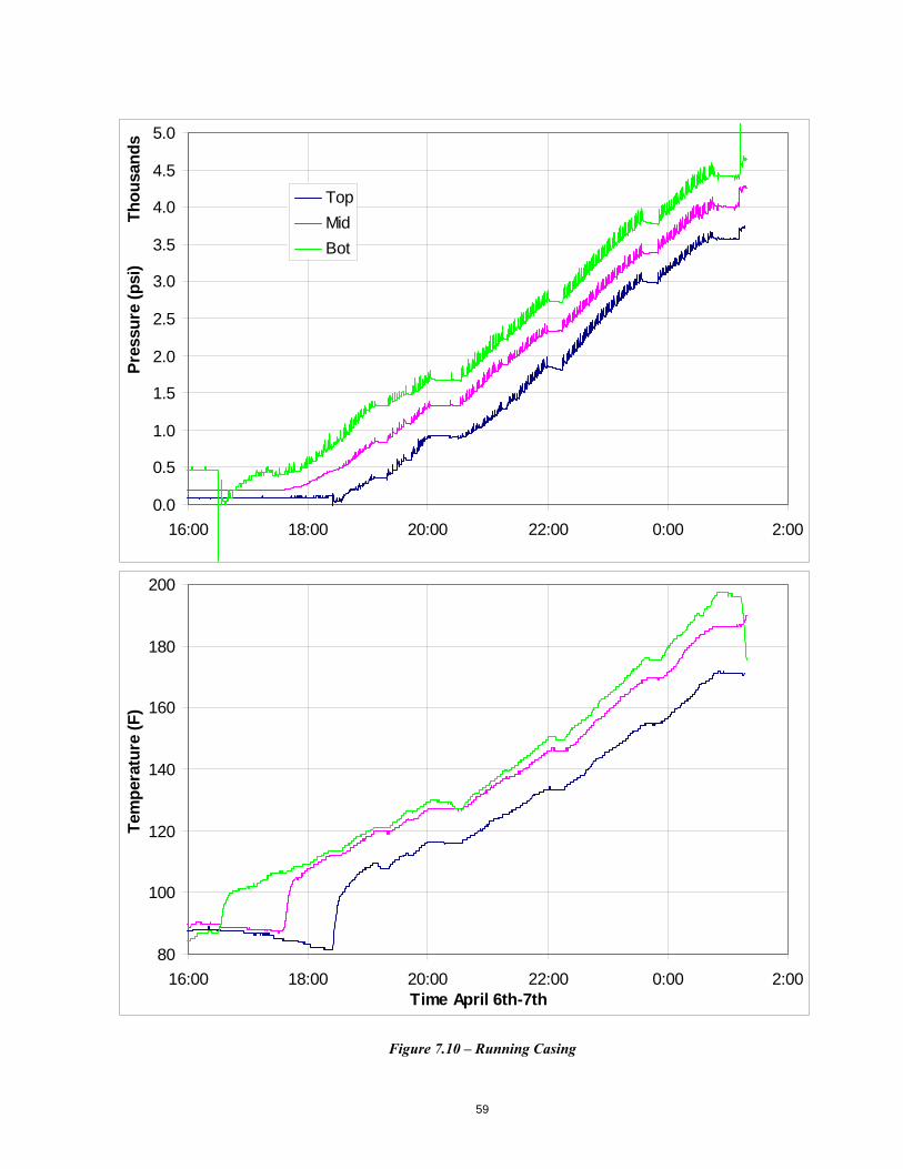
59

Figure 7.10 – Running Casing

0.0

0.5

1.0

1.5

2.0

2.5

3.0

3.5

4.0

4.5

5.0

16:00 18:00 20:00 22:00 0:00 2:00

Th

ou

san

ds

Pre

ssu

re (

psi

)

Top

Mid

Bot

80

100

120

140

160

180

200

16:00 18:00 20:00 22:00 0:00 2:00Time April 6th-7th

Tem

per

atu

re (

F)

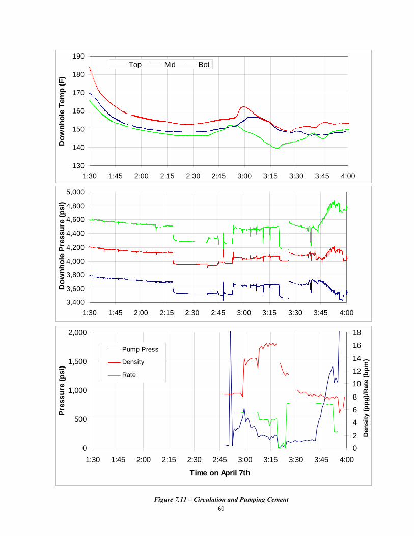
60 Figure 7.11 – Circulation and Pumping Cement

130

140

150

160

170

180

190

1:30 1:45 2:00 2:15 2:30 2:45 3:00 3:15 3:30 3:45 4:00

Do

wn

ho

le T

emp

(F

)Top Mid Bot

3,400

3,600

3,800

4,000

4,200

4,400

4,600

4,800

5,000

1:30 1:45 2:00 2:15 2:30 2:45 3:00 3:15 3:30 3:45 4:00

Do

wn

ho

le P

ress

ure

(p

si)

0

500

1,000

1,500

2,000

1:30 1:45 2:00 2:15 2:30 2:45 3:00 3:15 3:30 3:45 4:00

Time on April 7th

Pre

ssu

re (

psi

)

0

2

4

6

8

10

12

14

16

18

Den

sity

(p

pg

)/R

ate

(bp

m)

Pump Press

Density

Rate

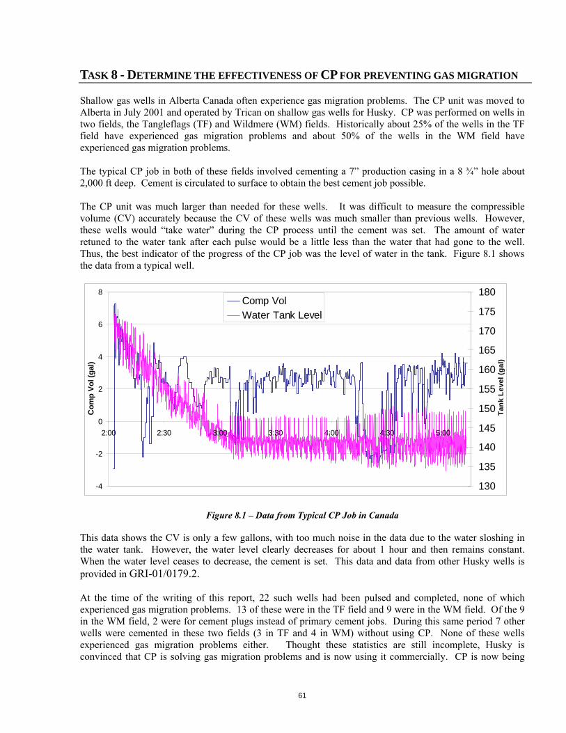
61

TASK 8 - DETERMINE THE EFFECTIVENESS OF CP FOR PREVENTING GAS MIGRATION

Shallow gas wells in Alberta Canada often experience gas migration problems. The CP unit was moved to Alberta in July 2001 and operated by Trican on shallow gas wells for Husky. CP was performed on wells in two fields, the Tangleflags (TF) and Wildmere (WM) fields. Historically about 25% of the wells in the TF field have experienced gas migration problems and about 50% of the wells in the WM field have experienced gas migration problems. The typical CP job in both of these fields involved cementing a 7” production casing in a 8 ¾” hole about 2,000 ft deep. Cement is circulated to surface to obtain the best cement job possible. The CP unit was much larger than needed for these wells. It was difficult to measure the compressible volume (CV) accurately because the CV of these wells was much smaller than previous wells. However, these wells would “take water” during the CP process until the cement was set. The amount of water retuned to the water tank after each pulse would be a little less than the water that had gone to the well. Thus, the best indicator of the progress of the CP job was the level of water in the tank. Figure 8.1 shows the data from a typical well.

Figure 8.1 – Data from Typical CP Job in Canada

This data shows the CV is only a few gallons, with too much noise in the data due to the water sloshing in the water tank. However, the water level clearly decreases for about 1 hour and then remains constant. When the water level ceases to decrease, the cement is set. This data and data from other Husky wells is provided in GRI-01/0179.2. At the time of the writing of this report, 22 such wells had been pulsed and completed, none of which experienced gas migration problems. 13 of these were in the TF field and 9 were in the WM field. Of the 9 in the WM field, 2 were for cement plugs instead of primary cement jobs. During this same period 7 other wells were cemented in these two fields (3 in TF and 4 in WM) without using CP. None of these wells experienced gas migration problems either. Thought these statistics are still incomplete, Husky is convinced that CP is solving gas migration problems and is now using it commercially. CP is now being

-4

-2

0

2

4

6

8

2:00 2:30 3:00 3:30 4:00 4:30 5:00

Co

mp

Vo

l (g

al)

130

135

140

145

150

155

160

165

170

175

180

Ta

nk

Le

ve

l (g

al)

Comp Vol

Water Tank Level

62

performed in another field in which 100% of all wells have leaked. Results from this third field are not yet available. More statistics will be published when the wells are completed.

63

TASK 9 - METHODS FOR CP ANALYSIS, DESIGN, AND CONTROL

Methods and Mathematical Models for CP Design and Control Submitted by: Andrew K. Wojtanowicz Craft and Hawkins Department of Petroleum Engineering Louisiana State University Baton Rouge, Louisiana August 19, 2001

TASK OBJECTIVE

Objective of Task 9 was to describe analytically the process of CP treatment and create a method to design the process. Specifically, the objective should be accomplished in the following steps:

Analyze physical principles of the CP process and simplify the process for the purpose of modeling; Develop analytical expressions describing stress (pressure)-strain(displacement) mechanism in the

CP process; Formulate mathematical model of CP describing pressure pulse transmission and displacemnt

amplitude distribution vs. depth and time; Define treatment depth; Verify the model in full-scale experiments; Develop a CP design model - an algorithm for designing CP treatments in wells with known

properties of annulus, drilling fluid and cement slurries; Validate the design model using field data from CP treatments in wells.

PHYSICAL ANALYSIS OF THE CP PROCESS Efficient transmission of small top pressure pulses over several thousand feet down the annular column of Non-Newtonian fluids with yield stress could only be efficient if the column yields only at the walls while the bulk fluid remains not sheared. From the analysis of flow of Bingham fluid in the annulus (Thesis,Section 2.1.1) it has become clear that velocities required to shear the whole volume such that there is no plug within the annular fluid are very high and practically un attainable. Thus, the model employs the plug flow concept and formulas to describe partial attenuation of pressure in the annulus. Moreover, since the slurry moves only as a plug its reciprocating motion can be converted to an equivalent slow continuous motion in the plug flow regime. After a few modeling attempts aimed at pressure wave propagation and other effects of pressure transient the modeling focused on a pseudo dynamic concept where the velocity of the fluid and the deformation of the annular walls is considered, while the transient effects are neglected. The simplification is based on evaluation of the pressure pulse propagation velocity in the annular system (Thesis, Appendix A) for different annular sizes. It was found that the velocity of pressure wave in the annulus would range between 2500 ft/second to 4200 ft/sec. As the typical pressure pulse duration used in TCP is of the order of the 10’ s of seconds and the velocity of pulse application is low the pressure transients are negligible. During the CP operation cement slurry at depth is sheared at the walls as it reciprocates upwards and downwards. As the annulus is a closed system the slurry movement in the annulus is caused by elastic deformation of the fluid and the annular walls. Thus, the displacement amplitude is caused by pressure at depth and controlled by compressibility of the annulus below this depth.

64

Designing of CP treatment for a well involves determination of parameters such as pressure pulse amplitude, pulse cycle duration, and the maximum depth of treatment. Interestingly, the three parameters are somewhat dependent on each other as well as they would obviously relate to the properties of cement, mud, rock, and annular geometry of the well. Hence, mathematical modeling of pressure pulse transmission (attenuation) becomes a basis for the design. The applied pressure is “spent” on overcoming system compressibility and frictional force. In the modeling we do not quantify the effect of shearing rate on slurry gelation process. Based on our experiments (Manowski Thesis, and Martin Thesis) we assume that as long as the slurry is sheared at the wall its gelation is effectively retarded disregarding the shearing rate value. Thus, the CP treatment is effective when pressure value at depth exceeds the time-dependent value of static gel strength of the slurry. The condition would define the depth of (effective) treatment.

PLUG FLOW PRESSURE GRADIENT Movement of annular fluid during CP has been described using the Bingham fluid flow model. The model has been improved for accuracy by removing the conventional assumption that the shear stress at wall is more than twice the yield of the fluid. The modification resulted in a non-linear (cubic) flow equation. Since this equation does not have an analytical solution an approximate solution has been derived. The approximation requires that conventional equation for frictional losses is multiplied by a correction factor and is very easy to use in the closed-form. Moreover, validity of the approximation has been evaluated and found suitable for CP computations.

COMPRESSIBILITY OF CEMENTED WELL ANNULUS

Included in this task is the derivation of expressions for finding compressibility of the annular system for openhole, cased hole and for the open hole with several rock layers having different properties. The compressibility expressions relate elastic properties of the material on the annular walls (rock and steel), compressibility of the fluids and geometry of the annulus to the value of applied pressure pulse and resulting volume change. The system compressibility for the whole annulus consisting of both open hole and cased hole sections has been calculated by taking the volume-weighted average of the individual section compressibilities. A procedure has been also developed for computing elastic properties of the rock (Poisson Ratio and Young’s Modulus) using empirical correlations. An example demonstrates the procedure for a hypothetical well in the Gulf Coast area.

MATHEMATICAL MODEL OF CP PULSE TRANSMISSION Derivation of the mathematical model is based on the following assumptions:

Reciprocating motion of slurry is represented by equivalent continuous motion with average velocity (Thesis, Equ. 4.1);

The annular fluids follow Bingham plastic model in plug flow; System compressibility applies and the annular system behaves elastically; Pressure pulse duration is sufficiently long so inertial effects can be neglected; Time dependent slurry properties (yield stress and plastic viscosity are known; The applied top pressure is balanced by the total distributed friction due to slurry movement; i.e

frictional pressure loss in plug flow controls pressure transmission downhole;

65

Duration of time lapse between the two consecutive pulses is sufficiently long so that the stress from the previous pulse fully diminishes; i.e. displacement amplitude is not affected by residual stresses;

There is an active mechanism of stress relaxation in the annular fluid column – fluid loss to the rock; Displacement amplitude is distributed and it depends on the compressibility and pressure

distributions. Based upon these assumptions, equivalent velocity is given by the formula:

fzyzv *)(2

1)( …………………………………………………………………….(4.1)

The top pressure pulse, p0, transmission formula is:

dzGvKpzp )()( 0 …………………………………………………..………...(4.2)

where:

12122

12

ln0614.0936.0)(200)(1000 dd

vC

dd

CG

dd

CK f

yfPf

and displacement amplitude is described by the equation:

)]1)[exp(1)(5.0)exp( cGzcpzczKfycpdz

dyoo (4.14)

which gives distributed displacement formula:

3)exp(

3)exp())exp(1()(

32

32

0

azzaz

aZZaZcpzy p

pp (4.17)

where:

)exp(25.0 0cpcKfa

From the model, the depth of CP treatment, Zt, and the top displacement amplitude, Y0, are calculated from the equation:

3)exp())exp(1(

32

0

taZZaZcpY pto (4.18)

by the method of iteration described in the Final Report (Thesis, Section 4.3, and 6). Finally, the bottomhole pressure at any time is computed as:

)21.4.....(..............................).........)(4

())(4

()(1212

tsp

tss Z

DDgZZ

DDgZp

The mathematical model was used to evaluate relative effect of the parameters involved in CP. The study revealed that:

Large well annuli improve pulse transmission significantly; There is almost linear increase of treatment depth with the size of top pressure pulse; Low-frequency pulses (f<0.1) would significantly increase treatment depth;

66

Annular system with large compressibility would slightly reduce treatment depth.

ALGORITHM FOR CP PROCESS DESIGN An algorithm and Excel spread sheet have been developed to design the CP process. The algorithm expands the mathematical model which was developed for an annular system with uniform and constant hole diameter, homogeneous single fluid. It uses the model to design CP in the systems with varying annular diameters, mud column above the cement, and cement columns having different gelling properties. Given the rock properties, fluid properties and well geometry the algorithm would calculate cement /mud top displacement, depth of treatment, and bottom hole pressure at any given point of time. As the computations are carried out in the step-wise manner until the cement setting time is reached, the output gives a complete description of the depth of treatment, top displacement amplitude, and bottomhole pressure vs. the treatment time. The algorithm has been structured in a modular format with the following modules: Compressibility module; Fluid property module; and, Cement pulsation module. The compressibility module computes the compressibility of the open hole and cased hole separately to be used then by the cement pulsation module to determine the system compressibility at each time step. An Excel spread sheet has been created to determine the cased hole compressibility using just one formula (Thesis, Eq. 3.23) The spread sheet uses equal values for fluid compressibility of the mud and cement slurry. Open hole compressibility is calculated using another Excel spread sheet, which calculates compressibility of each of the zones with different rock properties and annular sizes (Thesis, Eqs. 3.14, and 3.14), and then calculates the open hole compressibility (Thesis, Eqs. 3.15). In case the properties of the wellbore rocks are not known a default spread sheet for the Gulf Coast area could be used (Thesis, Fig. 6.4). The default-spread sheet utilizes the equations and correlations developed for the Gulf Coast area and returns just estimates of the Young’s modulus and Poisson’s ratio values to be used for finding estimated open hole compressibility. A flowchart of compressibility module’s algorithm (Thesis, Fig. 6.1) demonstrates the calculations. The fluid properties module calculates average property of the CP-treated annular fluid, at a particular point in time. The averaging transforms the actual system to an ideal one having uniform hole diameter and a single fluid with constant properties throughout the well.. The equivalent average property for the single fluid in a uniform hole diameter is calculated taking the volumetric averages of the properties of the actual fluid columns. Average hole diameter is computed, first. Then, the average YP and PV values are calculated using the following formulas (Thesis, Eqs. 6.1-6.3):

)3.6......(..........................................................................................)(300

)2.6.........(............................................................

)1.6......(............................................................

120

avg

avg

avg

YP

DDpZp

YPcLctLm

LctYPm

LctLm

LmYP

PVcLctLm

LctPVm

LctLm

LmPV

where: Zt = Lm + Lct

Equation 6.3 gives the first approximated depth of pressure pulse transmission which is a function of the average yield point. Hence equations 6.2 and 6.3 are iterated over the length of cement treated and the

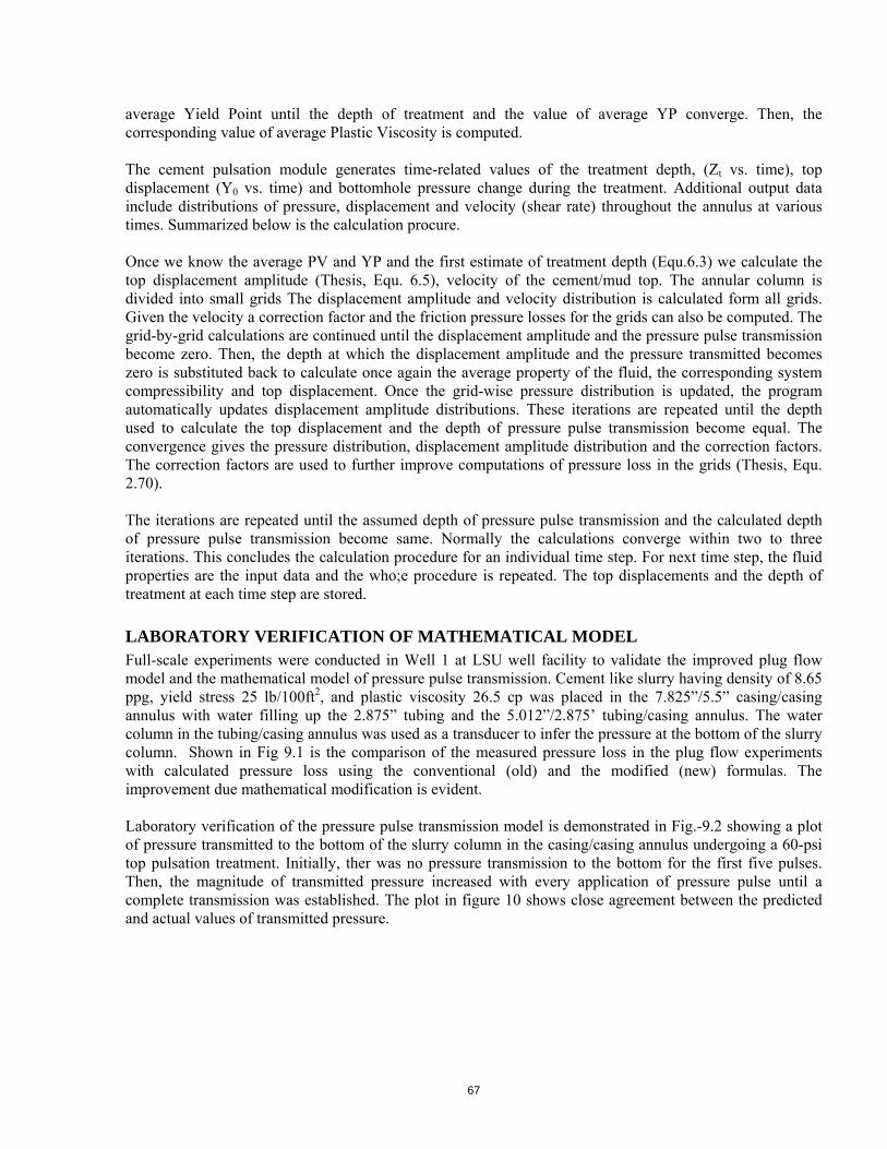
67

average Yield Point until the depth of treatment and the value of average YP converge. Then, the corresponding value of average Plastic Viscosity is computed. The cement pulsation module generates time-related values of the treatment depth, (Zt vs. time), top displacement (Y0 vs. time) and bottomhole pressure change during the treatment. Additional output data include distributions of pressure, displacement and velocity (shear rate) throughout the annulus at various times. Summarized below is the calculation procure. Once we know the average PV and YP and the first estimate of treatment depth (Equ.6.3) we calculate the top displacement amplitude (Thesis, Equ. 6.5), velocity of the cement/mud top. The annular column is divided into small grids The displacement amplitude and velocity distribution is calculated form all grids. Given the velocity a correction factor and the friction pressure losses for the grids can also be computed. The grid-by-grid calculations are continued until the displacement amplitude and the pressure pulse transmission become zero. Then, the depth at which the displacement amplitude and the pressure transmitted becomes zero is substituted back to calculate once again the average property of the fluid, the corresponding system compressibility and top displacement. Once the grid-wise pressure distribution is updated, the program automatically updates displacement amplitude distributions. These iterations are repeated until the depth used to calculate the top displacement and the depth of pressure pulse transmission become equal. The convergence gives the pressure distribution, displacement amplitude distribution and the correction factors. The correction factors are used to further improve computations of pressure loss in the grids (Thesis, Equ. 2.70). The iterations are repeated until the assumed depth of pressure pulse transmission and the calculated depth of pressure pulse transmission become same. Normally the calculations converge within two to three iterations. This concludes the calculation procedure for an individual time step. For next time step, the fluid properties are the input data and the who;e procedure is repeated. The top displacements and the depth of treatment at each time step are stored.

LABORATORY VERIFICATION OF MATHEMATICAL MODEL Full-scale experiments were conducted in Well 1 at LSU well facility to validate the improved plug flow model and the mathematical model of pressure pulse transmission. Cement like slurry having density of 8.65 ppg, yield stress 25 lb/100ft2, and plastic viscosity 26.5 cp was placed in the 7.825”/5.5” casing/casing annulus with water filling up the 2.875” tubing and the 5.012”/2.875’ tubing/casing annulus. The water column in the tubing/casing annulus was used as a transducer to infer the pressure at the bottom of the slurry column. Shown in Fig 9.1 is the comparison of the measured pressure loss in the plug flow experiments with calculated pressure loss using the conventional (old) and the modified (new) formulas. The improvement due mathematical modification is evident. Laboratory verification of the pressure pulse transmission model is demonstrated in Fig.-9.2 showing a plot of pressure transmitted to the bottom of the slurry column in the casing/casing annulus undergoing a 60-psi top pulsation treatment. Initially, ther was no pressure transmission to the bottom for the first five pulses. Then, the magnitude of transmitted pressure increased with every application of pressure pulse until a complete transmission was established. The plot in figure 10 shows close agreement between the predicted and actual values of transmitted pressure.

68

Figure 9.1 Plug Flow Model Comparison

Figure 9.2 Predicted vs Measured Pulses from LSU Well 1

VERIFICATION OF CP DESIGN MODEL WITH FIELD DATA To date, CTES – a lead investigator of the project – performed four cement pulsation field tests in non-instrumented wells (no down hole pressure sensors) and two tests in the instrumented wells with down hole

New model describes plug flow better than old model;LSU Well 1 flow experiments with Bingham slurry

0.015

0.02

0.0250.03

0.035

0.04

0.045

0.05

0.055

0.06

Time, minutes

Pre

ssu

re G

rad

ien

t p

si/f

t

New model

Measured

Old model

0 10 20 30 40 50

New model describes plug flow better than old model;LSU Well 1 flow experiments with Bingham slurry

0.015

0.02

0.0250.03

0.035

0.04

0.045

0.05

0.055

0.06

Time, minutes

Pre

ssu

re G

rad

ien

t p

si/f

t

New modelNew model

MeasuredMeasured

Old modelOld model

0 10 20 30 40 50

Mathematical model describes pulse pressure transmission;Pulsation experiment in LSU Well 1

0

5

10

15

20

25

30

0 5 10 15 20 25 30 35Pulse number

Pre

ssu

re, p

si

Pulsemeasured

Pulsepredicted

Pulsation stopped for 15 minutes

Mathematical model describes pulse pressure transmission;Pulsation experiment in LSU Well 1

0

5

10

15

20

25

30

0 5 10 15 20 25 30 35Pulse number

Pre

ssu

re, p

si

Pulsemeasured

Pulsepredicted

Pulsemeasured

Pulsepredicted

Pulsemeasured

Pulsepredicted

Pulsation stopped for 15 minutes

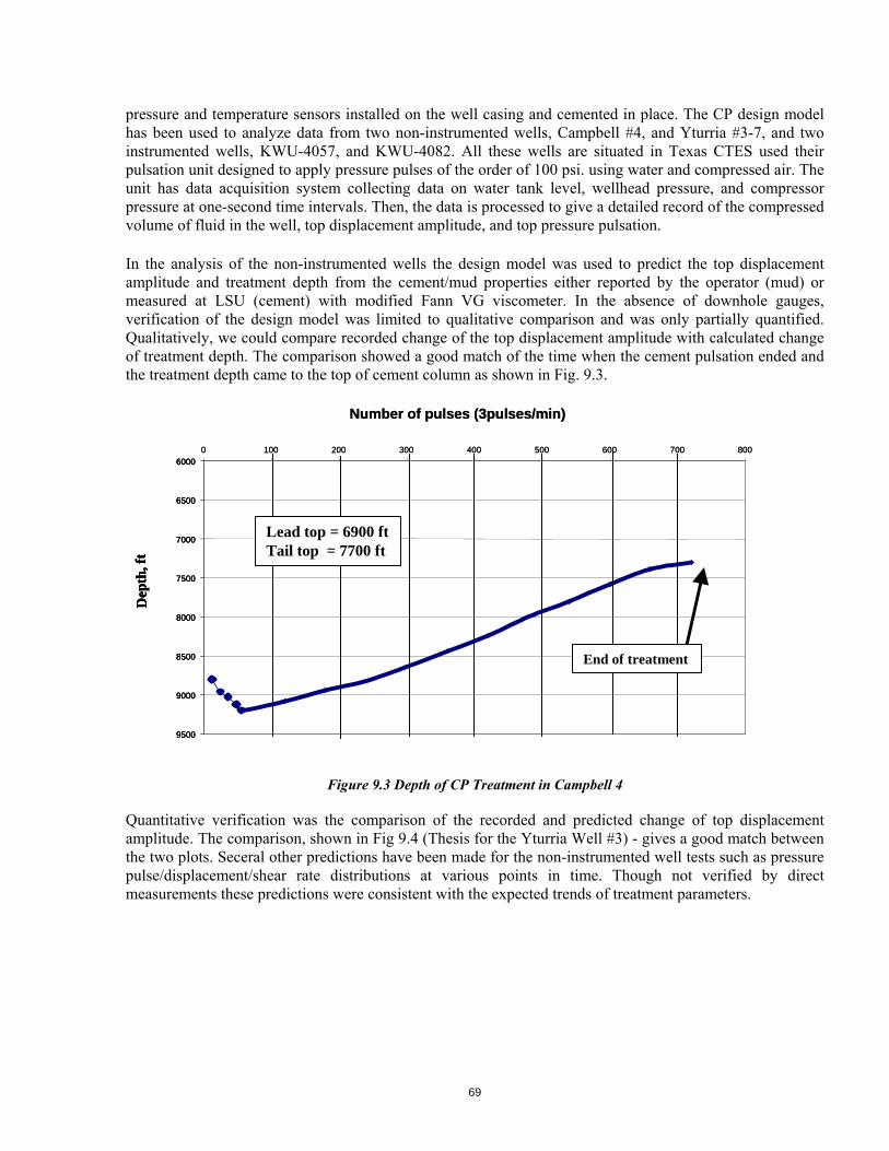
69

pressure and temperature sensors installed on the well casing and cemented in place. The CP design model has been used to analyze data from two non-instrumented wells, Campbell #4, and Yturria #3-7, and two instrumented wells, KWU-4057, and KWU-4082. All these wells are situated in Texas CTES used their pulsation unit designed to apply pressure pulses of the order of 100 psi. using water and compressed air. The unit has data acquisition system collecting data on water tank level, wellhead pressure, and compressor pressure at one-second time intervals. Then, the data is processed to give a detailed record of the compressed volume of fluid in the well, top displacement amplitude, and top pressure pulsation. In the analysis of the non-instrumented wells the design model was used to predict the top displacement amplitude and treatment depth from the cement/mud properties either reported by the operator (mud) or measured at LSU (cement) with modified Fann VG viscometer. In the absence of downhole gauges, verification of the design model was limited to qualitative comparison and was only partially quantified. Qualitatively, we could compare recorded change of the top displacement amplitude with calculated change of treatment depth. The comparison showed a good match of the time when the cement pulsation ended and the treatment depth came to the top of cement column as shown in Fig. 9.3.

Figure 9.3 Depth of CP Treatment in Campbell 4

Quantitative verification was the comparison of the recorded and predicted change of top displacement amplitude. The comparison, shown in Fig 9.4 (Thesis for the Yturria Well #3) - gives a good match between the two plots. Seceral other predictions have been made for the non-instrumented well tests such as pressure pulse/displacement/shear rate distributions at various points in time. Though not verified by direct measurements these predictions were consistent with the expected trends of treatment parameters.

0 100 200 300 400 500 600 700 800

Number of pulses (3pulses/min)

6000

6500

7000

7500

8000

8500

9000

9500

Dep

th, f

t

Lead top = 6900 ftTail top = 7700 ft

End of treatment

0 100 200 300 400 500 600 700 800

Number of pulses (3pulses/min)

6000

6500

7000

7500

8000

8500

9000

9500

Dep

th, f

t

6000

6500

7000

7500

8000

8500

9000

9500

Dep

th, f

t

Lead top = 6900 ftTail top = 7700 ft

End of treatment

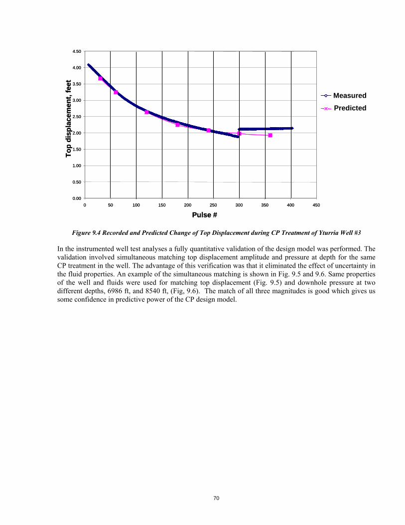
70

Figure 9.4 Recorded and Predicted Change of Top Displacement during CP Treatment of Yturria Well #3

In the instrumented well test analyses a fully quantitative validation of the design model was performed. The validation involved simultaneous matching top displacement amplitude and pressure at depth for the same CP treatment in the well. The advantage of this verification was that it eliminated the effect of uncertainty in the fluid properties. An example of the simultaneous matching is shown in Fig. 9.5 and 9.6. Same properties of the well and fluids were used for matching top displacement (Fig. 9.5) and downhole pressure at two different depths, 6986 ft, and 8540 ft, (Fig, 9.6). The match of all three magnitudes is good which gives us some confidence in predictive power of the CP design model.

0.00

0.50

1.00

1.50

2.00

2.50

3.00

3.50

4.00

4.50

0 50 100 150 200 250 300 350 400 450

Pulse #

To

p d

isp

lace

men

t, f

eet

Measured

Predicted

0.00

0.50

1.00

1.50

2.00

2.50

3.00

3.50

4.00

4.50

0 50 100 150 200 250 300 350 400 450

Pulse #

To

p d

isp

lace

men

t, f

eet

Measured

Predicted

MeasuredMeasured

Predicted

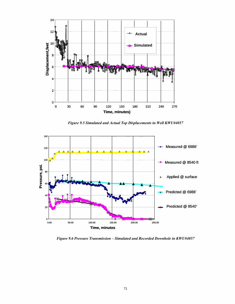
71

Figure 9.5 Simulated and Actual Top Displacements in Well KWU#4057

Figure 9.6 Pressure Transmission – Simulated and Recorded Downhole in KWU#4057

0

2

4

6

8

10

12

14

0 30 60 90 120 150 180 210 240 270

Time, minutes)

Dis

pla

cem

ent,

feet

Actual

Simulated

0

2

4

6

8

10

12

14

0 30 60 90 120 150 180 210 240 270

Time, minutes)

Dis

pla

cem

ent,

feet

Actual

Simulated

Actual

Simulated

0

20

40

60

80

100

120

140

0.00 50.00 100.00 150.00 200.00 250.00

Time, minutes

Pre

ssu

re, p

si.

Measured @ 6986’

Measured @ 8540 ft

Applied @ surface

Predicted @ 6986’

Predicted @ 8540’

0

20

40

60

80

100

120

140

0.00 50.00 100.00 150.00 200.00 250.00

Time, minutes

Pre

ssu

re, p

si.

Measured @ 6986’

Measured @ 8540 ft

Applied @ surface

Predicted @ 6986’

Predicted @ 8540’

72

TASK 10 – DIAGNOSTIC MODEL AND ANALYSIS METHOD FOR MONITORING PRESSURE

PULSE TRANSMISSION AND QUALITY OF CP TREATMENT

Task 10 Introduction The volumes of water pumped into the annulus and returned during TCP is monitored and converted to Top Cement Displacement Record (TCDR). TCDR is basically the same as the compressible volume (CV), discussed in other tasks of this paper, except it is measured in length units. The length is the displacement of the top of the cement. It had been postulated that TCDR might provide valuable information on the quality of cement setting in the annulus of the well. Consequently the record should some how be analyzed to determine fluid loss volume, initial/final position of top of cement and identify problems such as high fluid loss, bridging; identify presence of high temperature zones. The paper presents a diagnostic method based on recognition of TCDR patterns. From mathematical modeling of pulse transmission, different characteristic patterns have been derived. In the method the TCDR recorded from actual TCP data is compared with the expected TCDR. Then, a difference in the TCDR pattern between the expected and the actual TCDR is analyzed. From the analysis it can be determined what might have happened to the fluids placed in the annulus. The compressible volume of water pumped during each pulse into the annulus and thereby the depth of treatment depends on (1) system compressibility of the annulus as cement goes from liquid to solid state, (2) yield stress of fluids that are being treated, (3) fluid loss, and (4) cement Shrinkage. Cement shrinkage and fluid loss result in volume reduction and need additional volume to be pumped during pulsation. System compressibility during pulsation depends on (1) compressibility of cement and other fluids in the treated column, (2) compressibility due to ballooning of the outer casing, (3) compressibility due to compression of the inner casing, and (4) compressibility due to ballooning of the formation in the open hole.

Inverse Problem Solution A direct problem is one in which the known system and system inputs are used to find the output. An inverse problem is one in which the inputs and outputs are known whereas the system is unknown or only a few characteristics of the system are known. The known inputs and outputs can be used to find the response of the system. This type of a solution is called inverse problem solution. A well in which TCP is applied can be considered as an unknown system. The known input is the pulse pressure applied. The known output is the Top Cement Displacement Record (TCDR). The inverse problem solution in this case involves generating TCDR and using it to evaluate the cement setting process during pulsation. Figure 2 shows the approach to well diagnosis and the type of information that can be diagnosed about the system. Solution of the inverse problem is usually not unique. But the number of alternative solutions decreases as the number and the range of output signal measurements increase. Given below are the mathematical models that are needed for the diagnosis of well.

Mathematical Diagnostic Model In order to do the well diagnosis, the input, the output, and the known system properties should be linked using mathematical models as shown in figure 10.1. There are two mathematical models that can be used to do the well diagnosis. They are (1) pressure transmission model and (2) TCDR model. Pressure Transmission Model

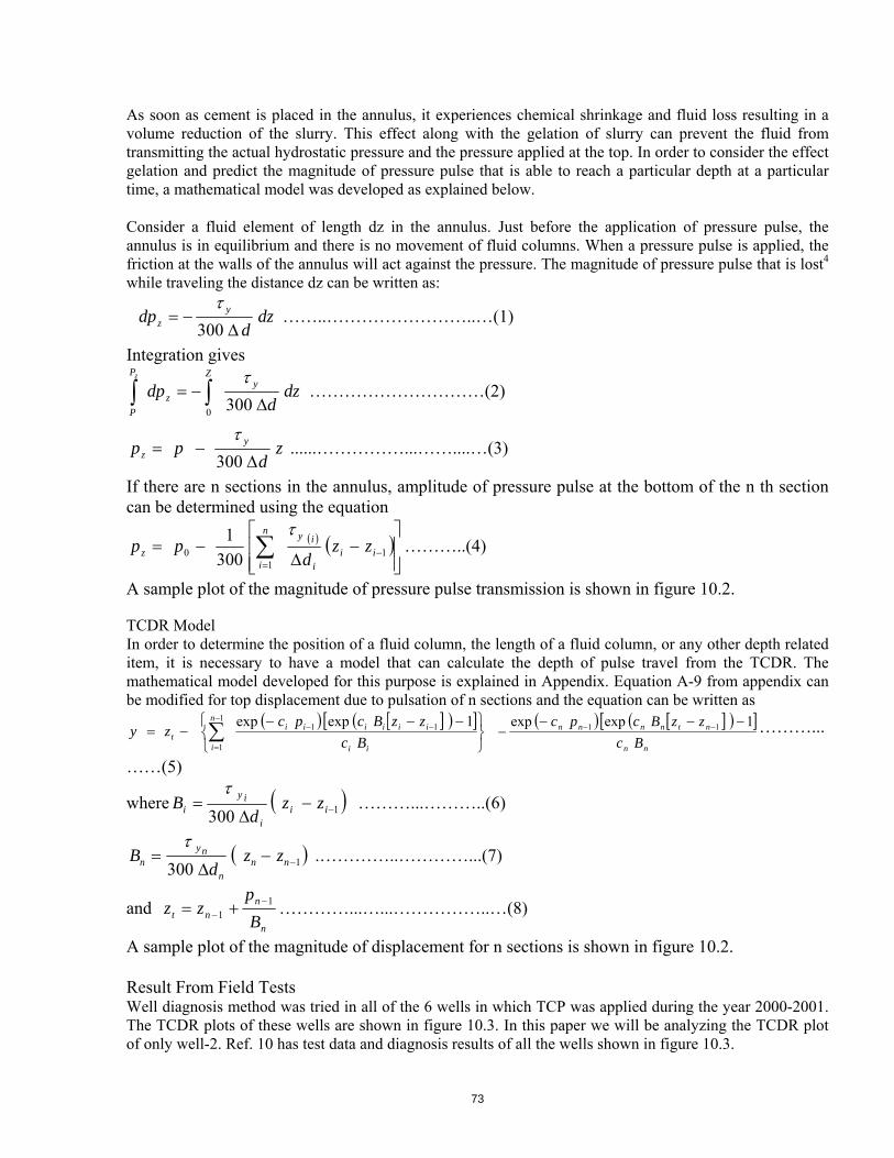
73

As soon as cement is placed in the annulus, it experiences chemical shrinkage and fluid loss resulting in a volume reduction of the slurry. This effect along with the gelation of slurry can prevent the fluid from transmitting the actual hydrostatic pressure and the pressure applied at the top. In order to consider the effect gelation and predict the magnitude of pressure pulse that is able to reach a particular depth at a particular time, a mathematical model was developed as explained below. Consider a fluid element of length dz in the annulus. Just before the application of pressure pulse, the annulus is in equilibrium and there is no movement of fluid columns. When a pressure pulse is applied, the friction at the walls of the annulus will act against the pressure. The magnitude of pressure pulse that is lost4 while traveling the distance dz can be written as:

dzd

dp yz

300

……..……………………..…(1)

Integration gives

dzd

dp yZ

z

P

P

z

3000

…………………………(2)

zd

pp yz

300

......……………...……....…(3)

If there are n sections in the annulus, amplitude of pressure pulse at the bottom of the n th section can be determined using the equation

1

10 300

1ii

i

iyn

iz zz

dpp

………..(4)

A sample plot of the magnitude of pressure pulse transmission is shown in figure 10.2. TCDR Model In order to determine the position of a fluid column, the length of a fluid column, or any other depth related item, it is necessary to have a model that can calculate the depth of pulse travel from the TCDR. The mathematical model developed for this purpose is explained in Appendix. Equation A-9 from appendix can be modified for top displacement due to pulsation of n sections and the equation can be written as

ii

iiiiiin

it Bc

zzBcpczy

1expexp 111

1

nn

ntnnnn

Bc

zzBcpc 1expexp 11 ………...

……(5)

where 1300

iii

iy

i zzd

B

………...………..(6)

1300

nnn

ny

n zzd

B

.…………..…………...(7)

and n

nnt B

pzz 1

1

…………...…...……………..…(8)

A sample plot of the magnitude of displacement for n sections is shown in figure 10.2. Result From Field Tests Well diagnosis method was tried in all of the 6 wells in which TCP was applied during the year 2000-2001. The TCDR plots of these wells are shown in figure 10.3. In this paper we will be analyzing the TCDR plot of only well-2. Ref. 10 has test data and diagnosis results of all the wells shown in figure 10.3.

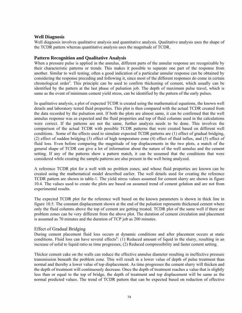
74

Well Diagnosis Well diagnosis involves qualitative analysis and quantitative analysis. Qualitative analysis uses the shape of the TCDR pattern whereas quantitative analysis uses the magnitude of TCDR. Pattern Recognition and Qualitative Analysis When a pressure pulse is applied in the annulus, different parts of the annular response are recognizable by their characteristic patterns or trends. This makes it possible to separate one part of the response from another. Similar to well testing, often a good indication of a particular annular response can be obtained by considering the response preceding and following it, since most of the different responses do come in certain chronological order5. This principle can be used to confirm thickening of cement, which usually can be identified by the pattern at the last phase of pulsation job. The depth of maximum pulse travel, which is same as the event of minimum cement yield stress, can be identified by the pattern of the early pulses. In qualitative analysis, a plot of expected TCDR is created using the mathematical equations, the known well details and laboratory tested fluid properties. This plot is then compared with the actual TCDR created from the data recorded by the pulsation unit. If both the plots are almost same, it can be confirmed that the well annulus response was as expected and the fluid properties and top of fluid columns used in the calculations were correct. If the patterns are not the same, further analysis needs to be done. This involves the comparison of the actual TCDR with possible TCDR patterns that were created based on different well conditions. Some of the effects used to simulate expected TCDR patterns are (1) effect of gradual bridging, (2) effect of sudden bridging (3) effect of high temperature zone (4) effect of fluid influx, and (5) effect of fluid loss. Even before comparing the magnitude of top displacements in the two plots, a match of the general shape of TCDR can give a lot of information about the nature of the well annulus and the cement setting. If any of the patterns show a pattern match, it can be assumed that the conditions that were considered while creating the sample patterns are also present in the well being analyzed. A reference TCDR plot for a well with no problem zones, and whose fluid properties are known can be created using the mathematical model described earlier. The well details used for creating the reference TCDR pattern are shown in table-1. The yield stress values assumed for cement slurry are shown in figure 10.4. The values used to create the plots are based on assumed trend of cement gelation and are not from experimental results. The expected TCDR plot for the reference well based on the known parameters is shown in thick line in figure 10.5. The constant displacement shown at the end of the pulsation represents thickened cement where only the fluid columns above the top of cement are getting treated. TCDR plot of the same well if there are problem zones can be very different from the above plot. The duration of cement circulation and placement is assumed as 70 minutes and the duration of TCP job as 200 minutes.

Effect of Gradual Bridging During cement placement fluid loss occurs at dynamic conditions and after placement occurs at static conditions. Fluid loss can have several effects6: (1) Reduced amount of liquid in the slurry, resulting in an increase of solid to liquid ratio as time progresses, (2) Reduced compressibility and faster cement setting. Thicker cement cake on the walls can reduce the effective annulus diameter resulting in ineffective pressure transmission beneath the problem zone. This will result in a lower value of depth of pulse treatment than normal and thereby a lower value of top displacement. As time progresses the cement slurry will thicken and the depth of treatment will continuously decrease. Once the depth of treatment reaches a value that is slightly less than or equal to the top of bridge, the depth of treatment and top displacement will be same as the normal predicted values. The trend of TCDR pattern that can be expected based on reduction of effective

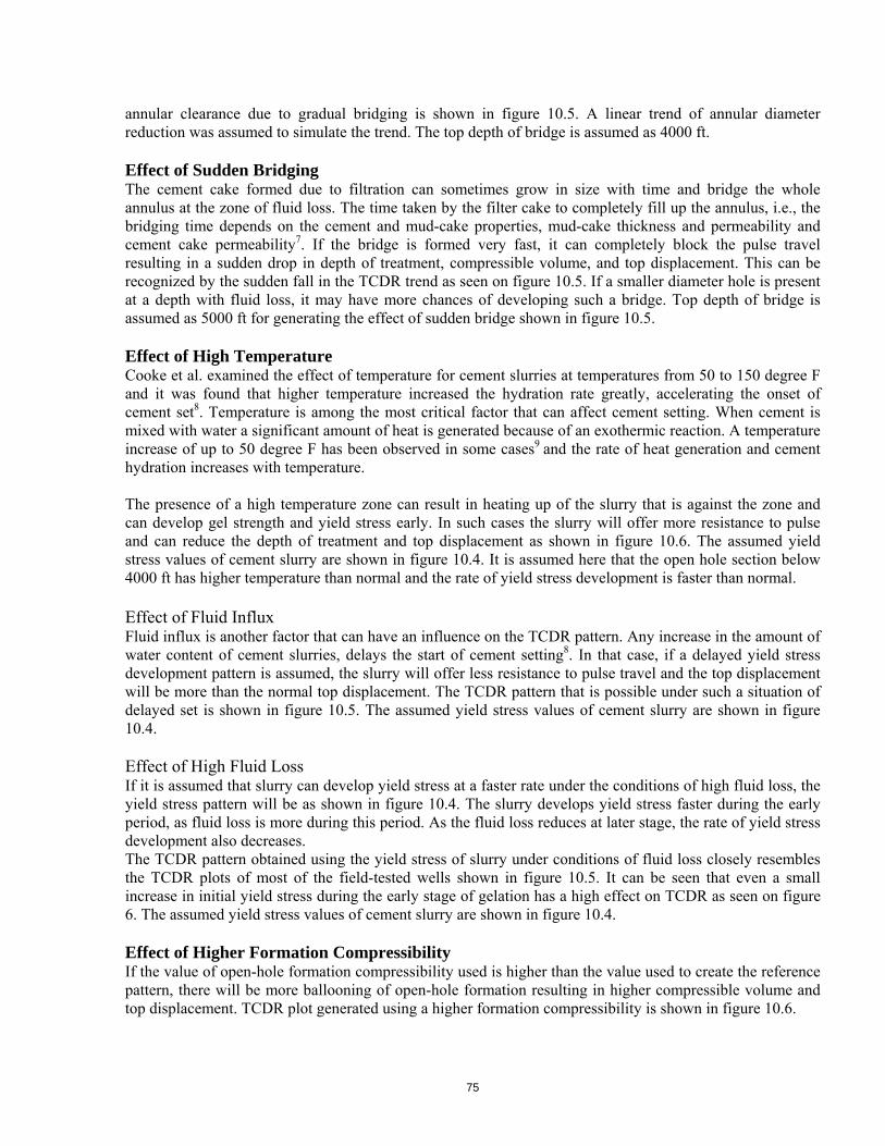
75

annular clearance due to gradual bridging is shown in figure 10.5. A linear trend of annular diameter reduction was assumed to simulate the trend. The top depth of bridge is assumed as 4000 ft. Effect of Sudden Bridging The cement cake formed due to filtration can sometimes grow in size with time and bridge the whole annulus at the zone of fluid loss. The time taken by the filter cake to completely fill up the annulus, i.e., the bridging time depends on the cement and mud-cake properties, mud-cake thickness and permeability and cement cake permeability7. If the bridge is formed very fast, it can completely block the pulse travel resulting in a sudden drop in depth of treatment, compressible volume, and top displacement. This can be recognized by the sudden fall in the TCDR trend as seen on figure 10.5. If a smaller diameter hole is present at a depth with fluid loss, it may have more chances of developing such a bridge. Top depth of bridge is assumed as 5000 ft for generating the effect of sudden bridge shown in figure 10.5. Effect of High Temperature Cooke et al. examined the effect of temperature for cement slurries at temperatures from 50 to 150 degree F and it was found that higher temperature increased the hydration rate greatly, accelerating the onset of cement set8. Temperature is among the most critical factor that can affect cement setting. When cement is mixed with water a significant amount of heat is generated because of an exothermic reaction. A temperature increase of up to 50 degree F has been observed in some cases9 and the rate of heat generation and cement hydration increases with temperature. The presence of a high temperature zone can result in heating up of the slurry that is against the zone and can develop gel strength and yield stress early. In such cases the slurry will offer more resistance to pulse and can reduce the depth of treatment and top displacement as shown in figure 10.6. The assumed yield stress values of cement slurry are shown in figure 10.4. It is assumed here that the open hole section below 4000 ft has higher temperature than normal and the rate of yield stress development is faster than normal. Effect of Fluid Influx Fluid influx is another factor that can have an influence on the TCDR pattern. Any increase in the amount of water content of cement slurries, delays the start of cement setting8. In that case, if a delayed yield stress development pattern is assumed, the slurry will offer less resistance to pulse travel and the top displacement will be more than the normal top displacement. The TCDR pattern that is possible under such a situation of delayed set is shown in figure 10.5. The assumed yield stress values of cement slurry are shown in figure 10.4. Effect of High Fluid Loss If it is assumed that slurry can develop yield stress at a faster rate under the conditions of high fluid loss, the yield stress pattern will be as shown in figure 10.4. The slurry develops yield stress faster during the early period, as fluid loss is more during this period. As the fluid loss reduces at later stage, the rate of yield stress development also decreases. The TCDR pattern obtained using the yield stress of slurry under conditions of fluid loss closely resembles the TCDR plots of most of the field-tested wells shown in figure 10.5. It can be seen that even a small increase in initial yield stress during the early stage of gelation has a high effect on TCDR as seen on figure 6. The assumed yield stress values of cement slurry are shown in figure 10.4. Effect of Higher Formation Compressibility If the value of open-hole formation compressibility used is higher than the value used to create the reference pattern, there will be more ballooning of open-hole formation resulting in higher compressible volume and top displacement. TCDR plot generated using a higher formation compressibility is shown in figure 10.6.

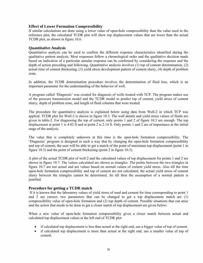
76

Effect of Lower Formation Compressibility If similar calculations are done using a lower value of open-hole compressibility than the value used in the reference plot, the calculated TCDR plot will show top displacement values that are lower than the actual TCDR plot, as shown in figure 10.6. Quantitative Analysis Quantitative analysis can be used to confirm the different response characteristics identified during the qualitative pattern analysis. Most responses follow a chronological order and the qualitative decision made based on indication of a particular annular response can be confirmed by considering the response and the depth of action preceding and following. Quantitative analysis involves (1) top of cement determination, (2) actual time of cement thickening, (3) yield stress development pattern of cement slurry, (4) depth of problem zone. In addition, the TCDR determination procedure involves the determination of fluid loss, which is an important parameter for the understanding of the behavior of well. A program called ‘Diagnosis’ was created for diagnosis of wells treated with TCP. The program makes use of the pressure transmission model and the TCDR model to predict top of cement, yield stress of cement slurry, depth of problem zone, and length of fluid columns that were treated. The procedure for quantitative analysis is explained below using data from Well-2 in which TCP was applied. TCDR plot for Well-2 is shown in figure 10.3. The well details and yield stress values of fluids are given in table-2. For diagnosing the top of cement, only points 1 and 2 of figure 10.3 are enough. The top displacement at point 1 is 4.02 ft and at point 2 is 2.14 ft. Only points 1 and 2 are of importance at the initial stage of the analysis. The value that is completely unknown at this time is the open-hole formation compressibility. The ‘Diagnosis’ program is designed in such a way that by changing the open-hole formation compressibility and top of cement, the user will be able to get a match of the point of maximum top displacement (point 1 in figure 10.3) and the point of cement thickening (point 2 in figure 10.3). A plot of the actual TCDR plot of well-2 and the calculated values of top displacement for points 1 and 2 are shown in figure 10.7. The values calculated are shown as triangles. The points between the two triangles in figure 10.7 are not actual and are values based on normal values of cement yield stress. Also till the time open-hole formation compressibility and top of cement are not calculated, the actual yield stress of cement slurry between the triangles cannot be determined. So till then the assumption of a normal pattern is justified. Procedure for getting a TCDR match If it is known that the laboratory values of yield stress of mud and cement for time corresponding to point 1 and 2 are correct, two parameters that can be changed to get a top displacement match are (1) compressibility value of open-hole formation and (2) top depth of cement. Possible situations that can arise and the action that needs to be done to get a closer match of top displacement are given below: When a new value of open-hole formation compressibility gives a closer match between actual and calculated top displacement values at the left end of TCDR plot

if calculated top displacement is less than actual at the right end, use a bigger value of top of cement. if calculated top displacement is more than actual at the right end, use a smaller value of top of

cement.

77

When a new value of open-hole formation compressibility gives a closer match between actual and calculated top displacement values at the right end of TCDR plot

if calculated top displacement is less than actual at the left end, use a smaller value of top of cement. if calculated top displacement is more than actual at the left end, use a bigger value of top of cement.

When a new value of top of cement gives a closer match between actual and calculated top displacement values at the left end of TCDR plot

if calculated top displacement is less than actual at the right end, use a bigger value of open-hole formation compressibility.

if calculated top displacement is more than actual at the right end, use a smaller value of open-hole formation compressibility.

When a new value of top of cement gives a closer match between actual and calculated top displacement values at the right end of TCDR plot

if calculated top displacement is less than actual at the left end, use a bigger value of open-hole formation compressibility.

if calculated top displacement is more than actual at the left end, use a smaller value of open-hole formation compressibility.

Using the above actions as guidelines, it is possible to find a closer match of point 1 and 2 of figure 10.7. Once a closer match is obtained the solver function of Excel can be used to find the top of cement value, till the actual and calculated top displacement values for point 1 and 2 match. A final plot of calculated TCDR that matches exactly with the actual TCDR is shown in figure 10.7. The compressibility of open-hole formation calculated is 5.3E-6 psi -1, and top of cement calculated is 3489 ft. Yield stress values of cement during TCP. Once the top of cement, and open-hole formation compressibility are known, the yield stress of cement at any time between point 1 and 2 can be easily calculated. The same ‘Diagnosis’ program can be used to calculate the yield stress by matching the actual and calculated top displacement of the point of interest. When all the points are matched, the calculated TCDR pattern will have the same magnitude and shape as the actual plot. Depth of problem zone The presence problem zones can be identified by pattern recognition and qualitative analysis method described earlier. Once the compressibility of open-hole formation and depth of top of cement are determined, the ‘Diagnosis’ program can be used to find the top of problem zone. If TCDR from a pulsation job looks like the one shown in figure 6, point P can be used to find the top of problem zone. The depth of pulsation and top depth of problem zone should be the same at point P. This is based on the fact that when the depth of pulsation starts to become less than the top of problem zone, the top displacement should match with the normal value of top displacement expected or calculated. The point at the beginning that corresponds to the start of pattern change from the actual top displacement gives the start time of problem. Fluid Loss The amount of fluid loss in the annulus can be calculated by finding the difference between the volume of water that was pumped into the annulus and the amount of water that came back from the annulus10. Length of Treated Fluid Column Once the formation compressibility and the top of cement are calculated, the length of fluid column that was treated by pulse at any time of interest can be calculated. This is done by finding the depth of treatment based on the top displacement at the point of interest.

78

Conclusions 1. All analyzed wells showed effects of fluid loss. 2. Actual yield stress development, affected by temperature and fluid loss has a high influence on the

top cement displacement record (TCDR) trend patterns. 3. Diagnosis method can be used as a tool to determine the top of cement and time of cement

thickening. 4. Diagnosis method can be used as a tool to determine the length of fluid column that was treated. 5. Diagnosis method can be used to determine the presence of any problem zones and their possible top

depth.

Nomenclature p = pressure, psi z = depth, ft τy = yield stress, lbf/ 100 sq. ft B = pressure reduction gradient, psi/ft c = compressibility, psi-1

d = difference in diameter, in

Subscripts z = depth i = index/ initial n = number of sections t = treatment References

1. Haberman, J.P., and Wolhart, S. L.: “Reciprocating Cement Slurries After Placement by Applying Pressure Pulses in the annulus,” SPE/IADC 37619, March 1997.

2. Martin, J.N.: “Laboratory and full-scale investigation of factors influencing the effectiveness of cement pulsation,” MS Thesis, LSU 2001.

3. Cooke, C.E., Gonzalez, O. J., and Broussard, D. J.: “Primary Cementing Improvement by Casing Vibration During Cement Curing time,” SPE 14199, 1985.

4. Bourgoyne, A.T., Chenvert, M.E., Millheim, K.K., and Young, F.S.: Applied Drilling Engineering, page 154, SPE textbook series,Vol. 2.

5. Horne, R.N.: Modern Well Test Analysis, 2nd edition, 1995. 6. Daccord, G. and Baret, J.F.: “How Fluid Loss Influences Primary Cementing: Literature review and

Methodology,” SPE 25150, 1994. 7. Baret, J.F.: “Why Cement Fluid Loss Additives are Necessary,” SPE 17630, 1988. 8. Chow, T.W., Mcintire, L.V., Kunze, K.R., and Cooke, C.E.: “The Rheological Properties of Cement

Slurries; Effects of Vibration, Hydration Conditions, and Additives,” SPE 13936, November 1988. 9. Romeo, J., and Loizzo, M.: “The importance of Hydration Heat on Cement Strength Development

for Deep Water Wells,” SPE 62894. 10. Kunju, M.R.: “Post-treatment diagnosis of cement pulsation in wells,” MS Thesis, LSU 2001.

Appendix—TCDR Model Bulk compressibility is defined as

dp

dV

Vc

1 …………………………...……….(A-1)

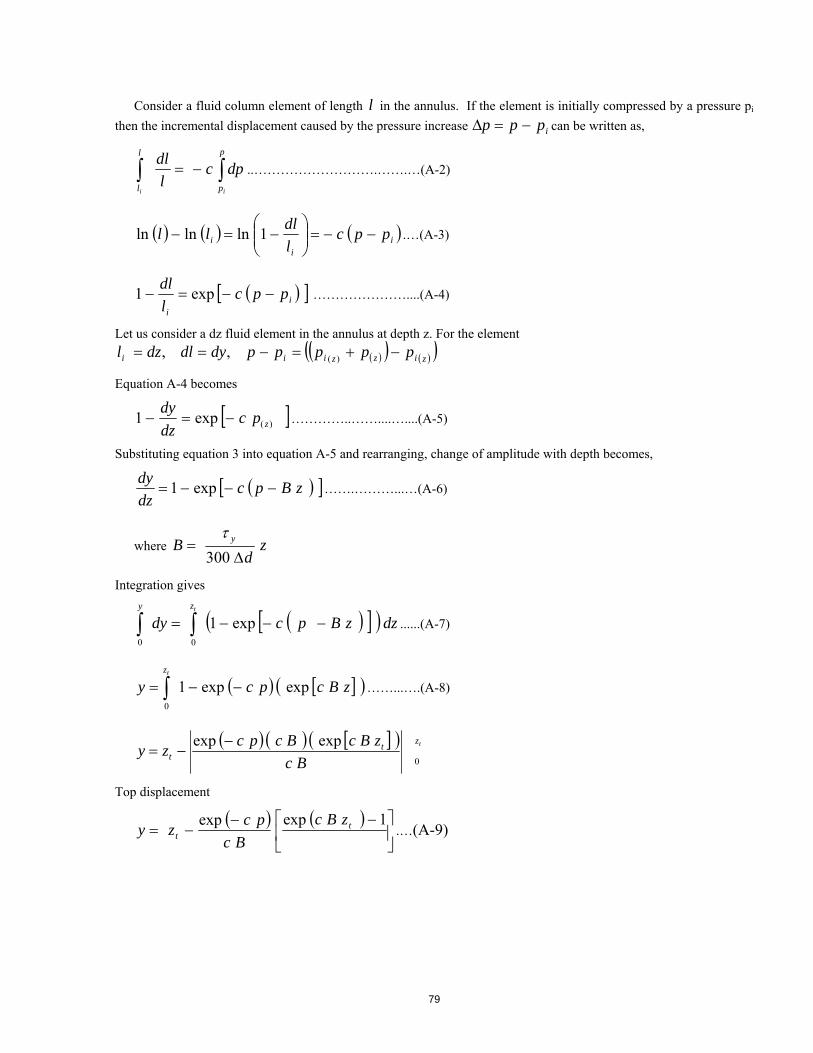
79

Consider a fluid column element of length l in the annulus. If the element is initially compressed by a pressure pi

then the incremental displacement caused by the pressure increase ippp can be written as,

p

p

l

l ii

dpcl

dl..……………………….…….…(A-2)

ii

i ppcl

dlll

1lnlnln .…(A-3)

ii

ppcl

dl exp1 …………………....(A-4)

Let us consider a dz fluid element in the annulus at depth z. For the element

zizziii pppppdydldzl )(,,

Equation A-4 becomes

)(exp1 zpcdz

dy …………..……....…....(A-5)

Substituting equation 3 into equation A-5 and rearranging, change of amplitude with depth becomes,

zBpcdz

dy exp1 …….………...…(A-6)

where zd

B y

300

Integration gives

dzzBpcdytzy

exp100

......(A-7)

zBcpcytz

expexp10

……...….(A-8)

tzt

t Bc

zBcBcpczy

0

expexp

Top displacement

1expexp tt

zBc

Bc

pczy .…(A-9)

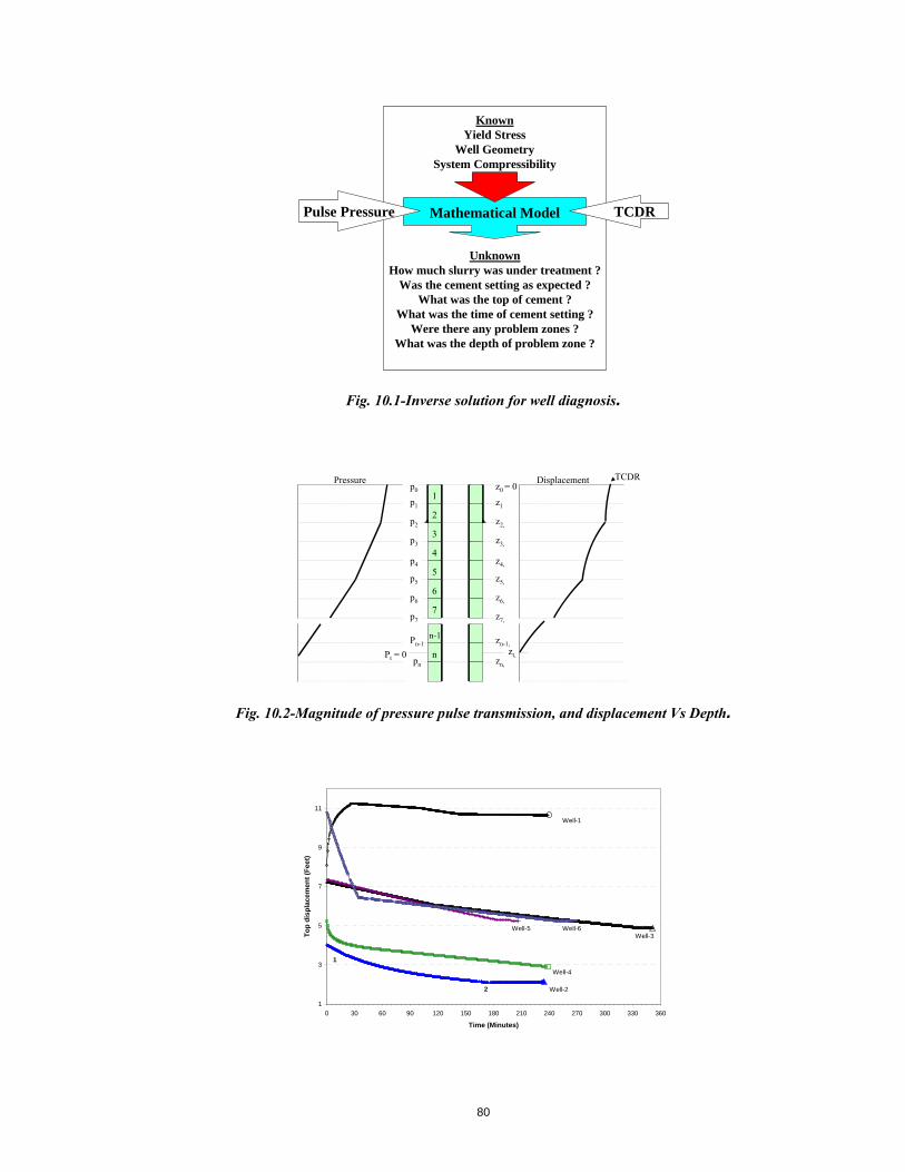
80

KnownYield Stress

Well GeometrySystem Compressibility

UnknownHow much slurry was under treatment ?

Was the cement setting as expected ?What was the top of cement ?

What was the time of cement setting ?Were there any problem zones ?

What was the depth of problem zone ?

Mathematical Model TCDRPulse Pressure

Fig. 10.1-Inverse solution for well diagnosis.

Pressure

z2,

z3,

z4,

z5,

z6,

z7,

zn-1,

zn,

zt,

1

2

3

4

5

6

7

n-1

z1p1

p2

p4

p5

p6

p7

Pn-1

Pt = 0pn

p3

p0 z0 = 0

n

Displacement TCDR

Fig. 10.2-Magnitude of pressure pulse transmission, and displacement Vs Depth.

1

3

5

7

9

11

0 30 60 90 120 150 180 210 240 270 300 330 360

Time (Minutes)

To

p d

isp

lace

men

t (F

eet)

Well-1

Well-2

Well-4

Well-5Well-3

Well-6

1

2

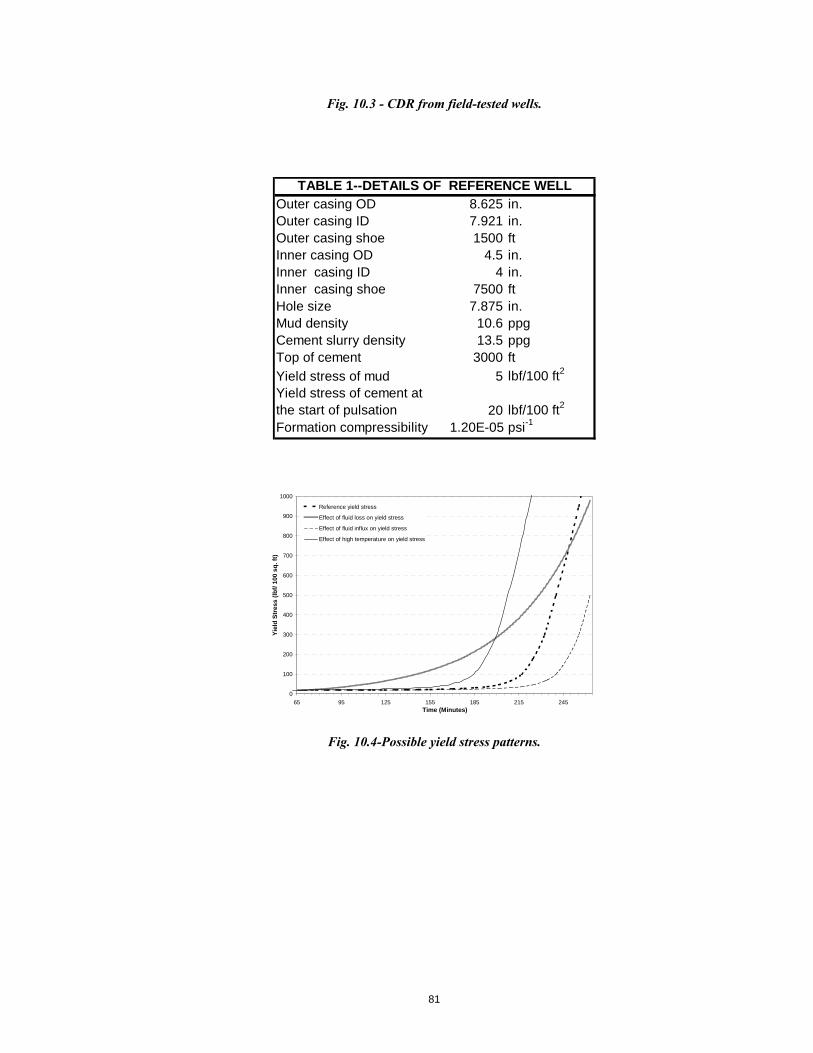
81

Fig. 10.3 - CDR from field-tested wells.

Outer casing OD 8.625 in.Outer casing ID 7.921 in.Outer casing shoe 1500 ftInner casing OD 4.5 in.Inner casing ID 4 in.Inner casing shoe 7500 ftHole size 7.875 in.Mud density 10.6 ppgCement slurry density 13.5 ppgTop of cement 3000 ft

Yield stress of mud 5 lbf/100 ft2

Yield stress of cement at the start of pulsation 20 lbf/100 ft2

Formation compressibility 1.20E-05 psi-1

TABLE 1--DETAILS OF REFERENCE WELL

0

100

200

300

400

500

600

700

800

900

1000

65 95 125 155 185 215 245Time (Minutes)

Yie

ld S

tres

s (l

bf/

100

sq

. ft)

Reference yield stress

Effect of fluid loss on yield stress

Effect of fluid influx on yield stress

Effect of high temperature on yield stress

Fig. 10.4-Possible yield stress patterns.

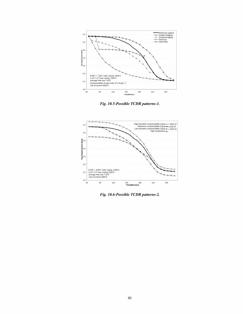
82

2.0

2.5

3.0

3.5

4.0

4.5

5.0

5.5

65 95 125 155 185 215 245

Time(Minutes)

To

p D

isp

acem

ent

(fee

t)

Reference patternSudden bridgingGradual bridgingFluid lossFluid influx

8 5/8" x 7.921" outer casing, 1500 ft4 1/2" x 4" inner casing, 7500 ftAverage hole size 7.875"

Compressibility of open hole 12 E-6 (psi -1) Top of cement 3000 ft

P

Fig. 10.5-Possible TCDR patterns-1.

2.0

2.5

3.0

3.5

4.0

4.5

5.0

5.5

65 95 125 155 185 215 245Time(Minutes)

To

p D

isp

acem

ent

(fee

t)

1.300E-05

1.20E-05

1.000E-05

High formation compressibility (1/psi)Reference compressibility (1/psi)

Low formation compressibility (1/psi)High temperature

8 5/8" x 8.097" outer casing, 1500 ft4 1/2" x 4" inner casing 7500 ftAverage hole size 7.875"Top of cement 3000 ft

Fig. 10.6-Possible TCDR patterns-2.

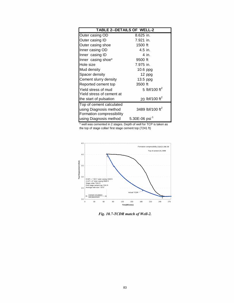
83

Outer casing OD 8.625 in.Outer casing ID 7.921 in.Outer casing shoe 1500 ftInner casing OD 4.5 in.Inner casing ID 4 in.Inner casing shoe* 9500 ftHole size 7.975 in.Mud density 10.6 ppgSpacer density 12 ppgCement slurry density 13.5 ppgReported cement top 3500 ft

Yield stress of mud 5 lbf/100 ft2

Yield stress of cement at the start of pulsation 20 lbf/100 ft2

Top of cement calculated using Diagnosis method 3489 lbf/100 ft2

Formation compressibility using Diagnosis method 5.30E-06 psi-1

TABLE 2--DETAILS OF WELL-2

* well was cemented in 2 stages. Depth of well for TCP is taken as the top of stage collar/ first stage cement top (7241 ft)

2.0

2.5

3.0

3.5

4.0

4.5

0 30 60 90 120 150 180 210 240 270

Time(Minutes)

To

p D

isp

ac

em

en

t (f

ee

t)

5.30E-06

3489

Formation compressibility (1/psi)

Top of cement (ft.)

1

2

8 5/8" x 7.921" outer casing 1500 ft4 1/2" x 4" inner casing 9500 ftStage collar 7241 ftFirst stage cement top 7241 ftAverage hole size 7.975"

Cement circulationand placement

Actual TCDR

Fig. 10.7-TCDR match of Well-2.

84

TASK 11 – LABORATORY EVALUATION OF CEMENT SLURRY FOR CP APPLICATIONS

Task Objective Develop a simple cement testing laboratory procedure to determine properties needed for CP design, monitoring and diagnosis. The procedure will provide input data to the models used in CP design and post-treatment analysis.

Test Protocol The following protocol for testing cements and drilling fluids prior to a cement pulsation job is proposed. These tests have two general purposes. The first is to verify the feasibility of cement pulsation and that up to 30 minutes downtime to hook up and begin pulsation will not cause excessive mud and cement gelation. The second is to measure the fluid properties for use with the CP model and in simple calculations to predict or analyze job performance. This protocol is intended to provide the same type of information for cement pulsation that conventional cement testing provides for a cement job. Descriptions of example tests performed on both mud and cement from an actual job are provided in Appendix 2, and example calculations using the test results are included herein.

Tests

Drilling Fluid (Mud): 1) Measure and record dial readings at 3, 6, 100, 200, 300, 600 rpm with standard Fann viscometer and

calculate YP3,6M and PVCPM. Use either the YP3,6M to make a quick prediction of pressure losses in mud column in annulus above cement or both for predictions using the CP model.

2) Measure and record 10 second, 10 minute, and 30 minute gel strengths. Cement: 1) Measure cement rheology at initiation of pulsation -- Prepare a sample of each slurry following API

Specification 10A. Condition each sample in an atmospheric consistometer with a temperature schedule versus time to simulate pumping time for proposed job. Remove sample from the consistometer and pour into a pre-heated, modified, twelve-speed Fann viscometer. The viscometer should be modified by using a knurled, 1.2276 cm radius bob with a standard F1 spring (an F2 spring and the appropriately revised equations can be used to double the maximum shear stress that can be measured, up to approximately 1500 lb/100sf). Measure 3, 6, 30, 60, 100, 200, 300 rpm dial readings and calculate YP3,6C and PVCPC. The YP3,6c can be used to make a quick prediction of pressure losses in cement column in the annulus at initial conditions. YP3,6C and PVCPC can similarly be used for predictions at initial conditions using the CP model. Measure and record 10 second and 10 minute gel strengths.

2) Measure static gel strength -- Prepare a sample of each slurry following API Specification 10A and condition each sample in a MACS Analyzer using the consistometer mode with temperature and pressure schedule and time to simulate pumping time for proposed job. Switch to the static gel strength (SGS) mode and measure SGS versus time, using a temperature schedule appropriate for cement curing. Continue for 30 minutes or until SGS = 500 lb/100sf, whichever occurs first. Optionally, measurements may continue if SGS is less than 500 lb/100sf and a measurement of SGS versus time is desired. This measurement provides a baseline prediction of SGS development if cement pulsation is not used.

3) Optional measurement of maximum treatment time -- Prepare a sample of each slurry following API Specification 10A and condition each sample in a MACS Analyzer using the consistometer mode with a

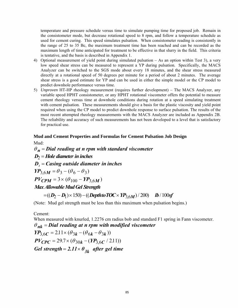
85

temperature and pressure schedule versus time to simulate pumping time for proposed job. Remain in the consistometer mode, but decrease rotational speed to 8 rpm, and follow a temperature schedule as used for cement curing. This speed simulates pulsation. When consistometer reading is consistently in the range of 25 to 35 Bc, the maximum treatment time has been reached and can be recorded as the maximum length of time anticipated for treatment to be effective in that slurry in the field. This criteria is tentative, and the basis is described in Appendix 1.

4) Optional measurement of yield point during simulated pulsation – As an option within Test 3), a very low speed shear stress can be measured to represent a YP during pulsation. Specifically, the MACS Analyzer can be switched to the SGS mode about every 18 minutes, and the shear stress measured directly at a rotational speed of 50 degrees per minute for a period of about 2 minutes. The average shear stress is a good estimate for YP and can be used in either the simple model or the CP model to predict downhole performance versus time.

5) Unproven HT-HP rheology measurement (requires further development) – The MACS Analyzer, any variable speed HPHT consistometer, or any HPHT rotational viscometer offers the potential to measure cement rheology versus time at downhole conditions during rotation at a speed simulating treatment with cement pulsation. These measurements should give a basis for the plastic viscosity and yield point required when using the CP model to predict downhole response to surface pulsation. The results of the most recent attempted rheology measurements with the MACS Analyzer are included as Appendix 2B. The reliability and accuracy of such measurements has not been developed to a level that is satisfactory for practical use.

Mud and Cement Properties and Formulas for Cement Pulsation Job Design

Mud: n Dial reading at n rpm with standard viscometer

D Hole diameter in inches2

inchesindiameteroutsideCasingD1

YP M3 6 3 6 3, ( )

PV YPCPM M 3 100 3 6( ),

Max Allowable MudGel Strength

D D DepthtoTOC YP lb sfM (( ) ) (( ) / ) /,2 1 3 6150 200 100

(Note: Mud gel strength must be less than this maximum when pulsation begins.) Cement: When measured with knurled, 1.2276 cm radius bob and standard F1 spring in Fann viscometer. nk Dial reading at n rpm with modified viscometer

YP C k k k3 6 3 6 3211, . ( ( ))

PV YPCPC k C 29 7 21130 3 6. ( ( / . )),

timegelafterθ2.11strengthGel 3k

86

Est Max Depthof Treatment Depth toTOC D D YP

DepthtoTOC YP D DC

M

. (( ( ) / )

( (( ) / ( ( )))),

,

300

100 3002 1 3 6

3 6 2 1

Max AllowableYP

D D DepthtoTOC YP lb sf

C

M

36

2 1 3 6150 200 100

,

,(( ) ) (( ) / ) /

Notes: 1) Cement yield point (or gel strength if cement pulsation has stopped) greater than this maximum will

prevent effective pulsation of any of the cement in the annulus. 2) All maximum values assume 100 psi pulse amplitude. 3) If the maximum depth of treatment is equal to or greater than the depth to the base of a lead slurry, the

length of the lead slurry can be added to the formula and the pressure lost in the lead slurry can be subtracted from the term that begins with 100.

Example Application of Testing Method to Fluids and Comparison to Field Results for KWU 4082

Example Calculation of Mud and Cement Properties

Mud: (from KWU #4057, no sample available from #4082) 3 2

6 2 5 .

100 14

D inches2 7875 .

D1 550 . inches

YP lb sfM3 6 2 2 5 2 15 100, ( . ) . /

PV cpCPM 3 14 15) 37 5( . .

Max Allowable Mud Gel Strength

lb sf (( . . ) ) (( . ) / ) /7875 550 150 6570 15 200 307 100

Cement: Measured with Fann viscometer using F1 spring and modified with knurled, 1.2276 cm radius bob, 3 11k

6 14k

30 17 3k estimated .

YP lb sfC3 6 211 11 14 11 16 9 100, . ( ( )) . /

PV cpCPC 29 7 17 3 16 9 211 276. ( . ( . / . ))

minutesafterlb/100sfstrengthGel 103617112 .

Est Max Depthof Treatment

ft

. (( ( . . ) / . )

( (( . ) / ( ( . . )))) ,

6570 300 7 875 550 16 9

100 6570 15 300 7 875 550 10 187

87

Note: This calculation is for the lead slurry. The top of the tail slurry was at 7725 feet, and total

depth was 8710 feet. Therefore this calculation is really only significant in the sense that it predicts

that pulsation will be effective over the entire length of lead slurry.

Max AllowableYP for pulsation or Cement Gel Strength when begin or resume pulsation

lb sfC36

7875 550 150 6570 15 200 307 100,

(( . . ) ) (( . ) / ) /

Comparison of Example Calculations to Field Results

Pulsation through the mud column Use of the calculated YP3,6M = 1.5 lb/100sf in the simple static equation proposed by Martin et al1 indicates that the pulse strength should be attenuated about 13 psi by the depth of the top pressure sensor. The attenuation reported in the field was 12 psi2. The calculated attenuation is 2.1 psi per 1000 feet of depth, which is comparable to the actual loss of 1.9 psi per 1000 feet of depth reported in the field. The 10 percent difference is well within the accuracy of measuring such small shear stresses with a rotational viscometer and of this simple model. Pulsation through the lead cement slurry column Use of the calculated initial YP3,6C = 17 lb/100sf in the simple static equation together with the measurements for the mud column allows prediction of pressure pulse amplitude at the middle pressure sensor at a depth of 7627 feet. The actual attenuation in the mud column to 6570 feet should be 12 psi. The initial attenuation in the cement slurry is estimated to be 25 psi for a total attenuation of 37 psi. The actual initial attenuation was reported to be 36 psi2. The calculated attenuation in the cement is 24 psi/1000 feet of depth, which is larger than the 19.1 psi per 1000 feet of depth reported in the field2. However, the pressure reported in the field indicates an attenuation rate of 22 psi/1000 feet of depth. In any event, use of YP3,6C results in better estimates of pressure pulse attenuation in the cement than conventional definitions of YP, YP3,6 measured with a standard viscometer, or YP estimated from the MACS Analyzer measurements described in Appendix 2B. The second part (Test 2) in the cement protocol is intended to determine static gel strength (SGS) development in the cement during the operational transition from the cement pumping job to cement pulsation. This test would be performed using the MACS Analyzer or other static gel strength measuring device. It was not conducted for this slurry. However, the average shear stress readings taken during a 5 minute pause in the simulated pulsation with the MACS Analyzer were from 211 to 300 lb/100sf and should be roughly equivalent to SGS. In addition, the gel strength measured with a viscometer after 10 minutes was 36 lb/100sf. Given that pulsation was in fact successful in the field when initiated within 4 minutes after the cement was placed, it is likely that the actual cement gel strength was considerably less than the “maximum allowed” value of 307 lb/100sf. Therefore the MACS Analyzer shear stress readings seem high in comparison to both the viscometer gel strengths measured at atmospheric pressure and the pulsation effectiveness in the field. A description of the overall complications encountered with the MACS Analyzer is included in Appendix 2B. Pulsation did support very effective pressure maintenance in the cement column of KWU #4082 for about 2 hours, but the pulse amplitude also decreased with time and eventually disappeared, see Figure 1. This is expected as the cement begins to cure and develops structure.

88

Figure 1 – Pulsation History for KWU 4082 Well

Attempts to simulate this behavior are the purpose of optional Cement Tests 3) and 4). While not conducted in exactly the same manner as proposed, results from a similar test simulating pulsation with the MACS Analyzer, see Figure 2 and Appendix 2B, do correspond roughly with results in the field. Specifically, low rpm consistency began increasing rapidly in the MACS Analyzer about 115 minutes after beginning simulated pulsation (at 175 minutes elapsed time). In the field, pulse amplitude gradually declined throughout the pulsation period indicating a progressive change in fluid properties downhole. However, an increase in the pulse amplitude attenuation rate and a decreasing trend in bottomhole pressure that occur about 120 minutes after pulsation began in the field seem to correlate with the change observed in the MACS Analyzer.

Figure 2 – Simulated Pulsation of KWU 4082 Lead Slurry in MACS Analyzer

Pulsation Period

KWU4082 Pressure Data

-

200

400

600

800

1,000

1,200

0:00 1:00 2:00 3:00 4:00 5:00 6:00 7:00

Time

Pre

ssur

e (p

si)

Mid - 3,100 psi

Top - 3,100 psi

Surf Press

Pulsation Test No. 1 - June 13, 2001 4,000 psi and 150 deg. F.

0

10

20

30

40

50

60

0 50 100 150 200 250

Elapsed Time (Minutes)

Co

nsi

sten

cy (

Bc)

0

20

40

60

80

100

120

140

160

180

Ro

tati

on

al S

pee

d (

rpm

) an

d T

emp

erat

ure

(F

)Max Consistency (BC)

Ave Consistency (BC)

Cell Wall Temp (F).

Rotation Speed (rpm)

Note increase in Consistency whenspeed slowed from 8 rpm to 4 rpm

Simulated Pumping Schedule

Simulated Pulsation

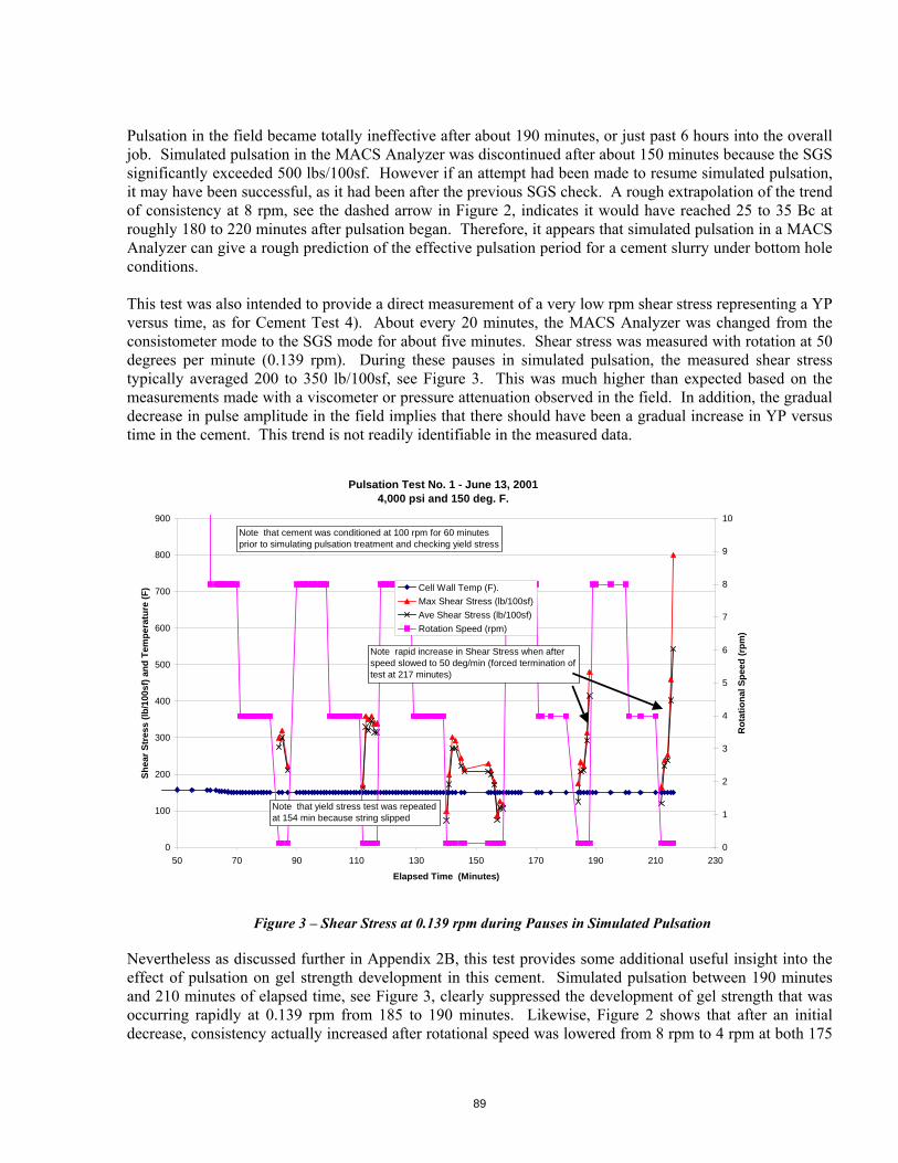
89

Pulsation in the field became totally ineffective after about 190 minutes, or just past 6 hours into the overall job. Simulated pulsation in the MACS Analyzer was discontinued after about 150 minutes because the SGS significantly exceeded 500 lbs/100sf. However if an attempt had been made to resume simulated pulsation, it may have been successful, as it had been after the previous SGS check. A rough extrapolation of the trend of consistency at 8 rpm, see the dashed arrow in Figure 2, indicates it would have reached 25 to 35 Bc at roughly 180 to 220 minutes after pulsation began. Therefore, it appears that simulated pulsation in a MACS Analyzer can give a rough prediction of the effective pulsation period for a cement slurry under bottom hole conditions. This test was also intended to provide a direct measurement of a very low rpm shear stress representing a YP versus time, as for Cement Test 4). About every 20 minutes, the MACS Analyzer was changed from the consistometer mode to the SGS mode for about five minutes. Shear stress was measured with rotation at 50 degrees per minute (0.139 rpm). During these pauses in simulated pulsation, the measured shear stress typically averaged 200 to 350 lb/100sf, see Figure 3. This was much higher than expected based on the measurements made with a viscometer or pressure attenuation observed in the field. In addition, the gradual decrease in pulse amplitude in the field implies that there should have been a gradual increase in YP versus time in the cement. This trend is not readily identifiable in the measured data.

Figure 3 – Shear Stress at 0.139 rpm during Pauses in Simulated Pulsation

Nevertheless as discussed further in Appendix 2B, this test provides some additional useful insight into the effect of pulsation on gel strength development in this cement. Simulated pulsation between 190 minutes and 210 minutes of elapsed time, see Figure 3, clearly suppressed the development of gel strength that was occurring rapidly at 0.139 rpm from 185 to 190 minutes. Likewise, Figure 2 shows that after an initial decrease, consistency actually increased after rotational speed was lowered from 8 rpm to 4 rpm at both 175

Pulsation Test No. 1 - June 13, 2001 4,000 psi and 150 deg. F.

0

100

200

300

400

500

600

700

800

900

50 70 90 110 130 150 170 190 210 230

Elapsed Time (Minutes)

Sh

ear

Str

ess

(lb

/100

sf)

and

Tem

per

atu

re (

F)

0

1

2

3

4

5

6

7

8

9

10

Ro

tati

on

al S

pee

d (

rpm

)

Cell Wall Temp (F).

Max Shear Stress (lb/100sf)

Ave Shear Stress (lb/100sf)

Rotation Speed (rpm)

Note rapid increase in Shear Stress when afterspeed slowed to 50 deg/min (forced termination of test at 217 minutes)

Note that cement was conditioned at 100 rpm for 60 minutesprior to simulating pulsation treatment and checking yield stress

Note that yield stress test was repeated at 154 min because string slipped

90

minutes and 200 minutes into the test. This gives evidence that there is some relationship between rate of gel strength development and shear rate or velocity of cement motion, at least near the cement setting period.

Summary and Conclusions 1) The fluid property definitions proposed herein provide a reasonable basis for simple predictions of

cement pulsation feasibility and performance. Specifically, the proposed YP criteria for the drilling fluid and cement can be used to predict attenuation and therefore pulse amplitude when cement pulsation is initiated. These criteria and gel strength also provide a basis for quick estimates of treatment depth and pulsation feasibility.

2) The proposed applications for the MACS Analyzer are not as well proven. However, the MACS Analyzer should be applicable for measuring cement static gel strength versus time under realistic conditions, as it was intended to do. In addition, it can be used at low rpm to simulate pulsation to determine an approximate maximum pulsation treatment time. It should also be useful for measuring YP during the pulsation period, but this application was not satisfactory in these tests. It may also be useful as a HTHP rheometer for cement pulsation, but that application is presently unreliable and requires additional development.

3) Results from the MACS Analyzer demonstrate that simulated pulsation does suppress and therefore delay development of cement gel strength. This effect was shown to be dependent on the velocity of the motion in the cement when the cement is close to setting. The opportunity to improve pulsation effectiveness near the end of a treatment by increasing pulsation frequency should be investigated.

91

TASK 12 – TRANSFER OF CP TECHNOLOGY TO INDUSTRY

The CP technology has been and is being transferred to the industry through presentations to interested groups such as the DEA and CEA, and through publication of the results. The publications to date are:

1. J. Martin, J.R. Smith, A. Wojtanowicz; “Experimental Assessment of Methods to Maintain Bottomhole Pressure After Cement Placement”, ETCE2001/DRILL-17133, ASME Engineering Technology Conference on Energy, Houston, February 2001

2. M. Kunju, A. Wojtanowicz; “Well Cementing Diagnosis From Top Cement Pulsation Record”, SPE 71387, SPE Annual Technical Conference and Exhibit, New Orleans, September 2001

3. K. Newman, A. Wojtanowicz, B. C. Gahan; “Cement Pulsation Improves Gas Well Cementing”, World Oil Magazine, July 2001

4. K. Newman, A. Wojtanowicz, B. C. Gahan; “Improving Gas Well Cement Jobs with Cement Pulsation”, GTI GasTIPS, Fall 2001, Volume 7, Number 3

The first 2 publications above are contained on the CD GRI-01/0179.2. Additional publications will be made as more statistical results are obtained from the commercial CP operation in Canada.