IMPROVEMENTS IN MAGNETIC RESONANCE

IMAGING USING INFORMATION REDUNDANCY

A Dissertation

Presented to the Faculty of the Graduate School

of Cornell University

in Partial Fulfillment of the Requirements for the Degree of

Doctor of Philosophy

by

Ashish Raj

May 2005

c© 2005 Ashish Raj

ALL RIGHTS RESERVED

IMPROVEMENTS IN MAGNETIC RESONANCE IMAGING USING

INFORMATION REDUNDANCY

Ashish Raj, Ph.D.

Cornell University 2005

This thesis describes a number of algorithms related to the acquisition, reconstruc-

tion and post-processing of Magnetic Resonance data. The basic theme underlying

each of these algorithms is the use of a unified systems approach to exploit infor-

mation redundancy available in MR imaging. There are three basic contributions.

The first concerns the development of a new motion correction algorithm for

Time-Resolved MR Angiography. Motion artifacts in angiography data are very

difficult to remove without affecting vascular evolution. Our algorithm uses suc-

cessive POCS iterations to remove unwanted artifacts without degrading quality.

Double-blind testing has indicated significant improvement over angiograms cre-

ated manually by experienced radiologist. In summary, our method seeks to exploit

temporal redundancy to remove motion artifacts.

The second contribution is our recent work on Parallel MR imaging in presence

of sensitivity errors using a Maximum Likelihood technique. It can be shown that

standard phased array reconstruction using popular parallel imaging methods is

inappropriate in presence of errors in measuring sensitivity maps of coils. Since

these errors are actually quite common and unavoidable, current reconstruction

methods can produce excessively noisy images. We describe a new algorithm that

uses a Maximum Likelihood formulation that is tolerant to such errors. Our results

indicate almost 20 dB improvement in SNR for noisy cases compared to standard

SENSE. In summary, this method effectively exploits receiver redundancy for res-

olution and scan time improvements.

The third major contribution involves exploiting prior information during the

reconstruction of parallel data in MR. We develop a Markovian field model for the

MR image prior and use it to perform Bayesian reconstruction of parallel data.

This involves solving a complicated energy function with extremely challenging

numerical properties. To make the approach practical, we have developed a fast

graph cut based energy minimization algorithm. It turns out that the same algo-

rithm is effective for all multi-dimensional problems involving linear systems with

non-negative elements. We thus generalize our method to cover a larger set of tar-

get problems, including image deconvolution, motion deblurring, etc. Our results

on reconstructed MR Angiography data suggests significant improvement in SNR

compared to standard SENSE reconstruction. Results for image deconvolution are

also very promising, and preliminary testing on several images has reported small

but significant gains in peak SNR. In summary, the graph cut approach is a natural

and powerful way to exploit spatial redundancy present in MR data.

Taken together, these contributions may have the potential to significantly alter

the current state of the art in MR imaging, especially MR angiography.

BIOGRAPHICAL SKETCH

Ashish Raj was born in Godda, India, in 1976. He received the B.E. degree in

Electrical and Electronic Engineering from the University of Auckland in 1998.

He joined the graduate program in Electrical Engineering at Cornell in the Fall of

1998, and received the M.S. degree in Electrical Engineering in 2001, specialising

in signal and image processing. Since then he has worked on medical imaging

problems, particularly MRI.

iii

ACKNOWLEDGEMENTS

First of all I would like to thank my advisor and mentor Professor Ramin Zabih

for his constant guidance and encouragement. He has helped me learn how to con-

duct independent research, while at the same time making judicious interventions

whenever I seemed to lose focus. His expertise and ”feel” for the issues involved

have greatly impacted my work and perhaps made up for some of my own short-

comings and lack of breadth. He has also done a marvelous job navigating several

bodies of terrifying bureaucracy on my behalf. I thank him for these and many

other ways he has guided me.

I would like to thank my parents for instilling in me an ethos and a culture of

academic pursuit. Without their guidance and encouragement this thesis could not

be written. I would like to thank Professors Thomas Parks, Dan Huttenlocher, Yi

Wang and Martin Prince for forming a very effective and constructive committee.

In particular Professors Wang and Prince deserve my unending gratitude for first

introducing me to this amazing field, and then extending every possible guidance

to help me understand the issues involved. I would like to acknowledge my col-

legues and fellow students Amy Gale, Junhwan Kim, Vladimir Kolmogorov, Pascal

Spincemaille, Bryan Kressler, Ryan Brown, Zhenghui Zhang and Darian Muresan

for many illuminating discussions. I thank Professor Charles Van Loan for his

suggestions on Total Least Squares techniques. Finally, thanks are due to ECE

administrative assistants Jamie Dal Cero and Cynthia Robinson who helped out

with countless little chores.

iv

TABLE OF CONTENTS

1 Introduction 11.1 Synopsis . . . . . . . . . . . . . . . . . . . . . . . . . . . . . . . . . 11.2 Why MRI? . . . . . . . . . . . . . . . . . . . . . . . . . . . . . . . 31.3 A unified view of the algorithmic problem in MR imaging . . . . . . 6

1.3.1 A linear systems approach to MR imaging . . . . . . . . . . 91.3.2 A summary of contributions . . . . . . . . . . . . . . . . . . 14

2 Introduction to MR Imaging 172.1 A brief introduction to MR imaging . . . . . . . . . . . . . . . . . . 17

2.1.1 Sampling k-space along trajectories . . . . . . . . . . . . . . 202.2 Accelerated scanning using parallel imaging . . . . . . . . . . . . . 22

2.2.1 System model . . . . . . . . . . . . . . . . . . . . . . . . . . 24

3 Motion Correction in Time-Resolved MR Angiography Using Con-vex Projections 283.1 Introduction . . . . . . . . . . . . . . . . . . . . . . . . . . . . . . . 293.2 Overview of Proposed Method . . . . . . . . . . . . . . . . . . . . . 31

3.2.1 Assumptions . . . . . . . . . . . . . . . . . . . . . . . . . . . 333.2.2 Related Work . . . . . . . . . . . . . . . . . . . . . . . . . . 33

3.3 POCS Based Motion Correction . . . . . . . . . . . . . . . . . . . . 363.3.1 P1 : K-space Box Constraint Step . . . . . . . . . . . . . . . 373.3.2 P2 : Phase Correction Step . . . . . . . . . . . . . . . . . . . 393.3.3 P3 : Parenchyma Correction Step . . . . . . . . . . . . . . . 413.3.4 P4 : Background Forcing Step . . . . . . . . . . . . . . . . . 41

3.4 A High-Pass Phase Filter for Suppression of Translation Artifacts . 423.4.1 Proof of Convexity of P2 . . . . . . . . . . . . . . . . . . . . 443.4.2 Phase Artifacts For a Piece-wise Motion Model . . . . . . . 463.4.3 Expression For Phase Difference . . . . . . . . . . . . . . . . 483.4.4 Special Case 1: K2 is small . . . . . . . . . . . . . . . . . . . 503.4.5 Special Case 2: K1 is small . . . . . . . . . . . . . . . . . . . 523.4.6 Special Case 3: K1 and K2 are equal . . . . . . . . . . . . . 52

3.5 Results . . . . . . . . . . . . . . . . . . . . . . . . . . . . . . . . . . 533.5.1 Materials and methods . . . . . . . . . . . . . . . . . . . . . 533.5.2 In-plane motion in a single frame: Simulation Results . . . . 543.5.3 Completely un-supervised clinical MR-DSA: a joint classifi-

cation and motion correction algorithm . . . . . . . . . . . . 613.5.4 Limitations and further improvements . . . . . . . . . . . . 65

3.6 Conclusion . . . . . . . . . . . . . . . . . . . . . . . . . . . . . . . . 67

v

4 Total Least Sense: A Maximum - Likelihood Approach to ParallelMR Imaging with Sensitivity Noise 684.1 Parallel Imaging and Sensitivity Noise . . . . . . . . . . . . . . . . 69

4.1.1 System matrix structure under Cartesian sampling . . . . . 714.1.2 System matrix structure under arbitrary sampling . . . . . . 744.1.3 Our noise model . . . . . . . . . . . . . . . . . . . . . . . . 74

4.2 Related Work . . . . . . . . . . . . . . . . . . . . . . . . . . . . . . 764.2.1 Total Least Squares . . . . . . . . . . . . . . . . . . . . . . . 764.2.2 Constrained Total Least Squares . . . . . . . . . . . . . . . 77

4.3 The TL-SENSE Algorithm . . . . . . . . . . . . . . . . . . . . . . . 784.3.1 Deriving the likelihood function (x) . . . . . . . . . . . . . 784.3.2 Minimization Algorithms . . . . . . . . . . . . . . . . . . . . 80

4.4 Results . . . . . . . . . . . . . . . . . . . . . . . . . . . . . . . . . . 834.4.1 Simulation results . . . . . . . . . . . . . . . . . . . . . . . . 834.4.2 Experiments with Sensitivity mismatch on phantom data . . 864.4.3 In vivo imaging with a 4-element torso coil array . . . . . . 884.4.4 Parallel Brain Imaging With An 8-Element Head Coil . . . . 92

4.5 Conclusions . . . . . . . . . . . . . . . . . . . . . . . . . . . . . . . 93

5 A Graph Cut Energy Minimization Algorithm for a New Class ofPixel Labeling Problems 975.1 Introduction . . . . . . . . . . . . . . . . . . . . . . . . . . . . . . . 97

5.1.1 Chapter Overview . . . . . . . . . . . . . . . . . . . . . . . . 995.2 Linear Inverse Problems in Machine Vision . . . . . . . . . . . . . . 99

5.2.1 Problem definition . . . . . . . . . . . . . . . . . . . . . . . 1015.3 Related Work . . . . . . . . . . . . . . . . . . . . . . . . . . . . . . 1015.4 Graph Cuts for H . . . . . . . . . . . . . . . . . . . . . . . . . . . . 1035.5 Approximating the Energy . . . . . . . . . . . . . . . . . . . . . . . 106

5.5.1 Further improvements . . . . . . . . . . . . . . . . . . . . . 1115.6 Experimental results - low level vision . . . . . . . . . . . . . . . . . 112

5.6.1 Deblurring Results . . . . . . . . . . . . . . . . . . . . . . . 1135.6.2 Motion Deblurring . . . . . . . . . . . . . . . . . . . . . . . 115

5.7 Graph Cuts in MR Reconstruction . . . . . . . . . . . . . . . . . . 1155.8 Experimental results on parallel MR . . . . . . . . . . . . . . . . . 1195.9 Extensions . . . . . . . . . . . . . . . . . . . . . . . . . . . . . . . . 120

6 Conclusions 1266.1 Extensions . . . . . . . . . . . . . . . . . . . . . . . . . . . . . . . . 128

6.1.1 TL-SENSE for arbitrary sampling . . . . . . . . . . . . . . . 1286.1.2 TL-SENSE for general noise models . . . . . . . . . . . . . . 1286.1.3 Graph Cut methods for arbitrary linear systems . . . . . . . 129

Bibliography 130

vi

LIST OF TABLES

3.1 Results of a Double Blind Comparison of Manual versus AutomaticPOCS Angiograms . . . . . . . . . . . . . . . . . . . . . . . . . . . 66

5.1 PSNR evaluation. Larger numbers indicate better performance(note that the measurements are in dB, so the scale is logarith-mic.) . . . . . . . . . . . . . . . . . . . . . . . . . . . . . . . . . . 117

vii

LIST OF FIGURES

1.1 Various sources of artifacts in MR imaging, and ways to removethem. . . . . . . . . . . . . . . . . . . . . . . . . . . . . . . . . . . 8

2.1 Schematic description of frequency- and phase-encoding steps usedto acquire k-space data. . . . . . . . . . . . . . . . . . . . . . . . . 20

2.2 Popular k-space trajectories. . . . . . . . . . . . . . . . . . . . . . 212.3 Schematic description of the parallel imaging process for the lth

coil. Note that the multiplication of X and Sl takes place pixel bypixel. . . . . . . . . . . . . . . . . . . . . . . . . . . . . . . . . . . 25

3.1 Overview of Motion Correction on MRA: the kth frame has motionartifacts, which are removed by the POCS algorithm by using thereference frame . . . . . . . . . . . . . . . . . . . . . . . . . . . . . 32

3.2 The POCS Motion Correction Algorithm: each box represents aconvex projection. . . . . . . . . . . . . . . . . . . . . . . . . . . . 37

3.3 The k-space box constraint imposed by P1 . . . . . . . . . . . . . . 383.4 A typical peripheral 2D MRA case (a) Original frame, image space,

(b) Difference image (c) Plot of k-space magnitudes vs. distance tocenter, and (d) ratio of vasculature magnitude to overall magnitude. 40

3.5 Typical power spectra of phase signals in k-space, obtained fromthe phase difference between consecutive frames: (a) Non-globaltranslation; (b) phase due to vasculature, obtained from an artifact-free sequence. . . . . . . . . . . . . . . . . . . . . . . . . . . . . . . 43

3.6 Frequency response of the high-pass phase filter. . . . . . . . . . . 433.7 Relationship between phase difference φ and translation phase

shift δ . . . . . . . . . . . . . . . . . . . . . . . . . . . . . . . . . 503.8 Averaged power spectra of phase signals: (a) Case A, α = |K2|/|K| =

0.2; (b) Case B, α = 0.9; (c) General intermediate case, α = 0.7. . . 513.9 Example of non-global step translation occurring in middle of k-

space acquisition: (a) Uncorrupted frame, (b) Corrupted frame,(c) Original angiogram, (d) Motion-corrupted angiogram, and (e)Corrected using POCS, with λ = 0.8 . . . . . . . . . . . . . . . . . 55

3.10 Motion Correction (a) Motion Corrupted Difference Image, and (b)Corrected using POCS Algorithm, with λ = 0.8 . . . . . . . . . . . 56

3.11 Non-global random-walk translation, plotted as a function of thephase encode index. The top curve shows translation in the PEdirection, while the bottom curve shows translation in FE direction. 57

3.12 Example of non-global random-walk translation occurring in mid-dle of k-space acquisition: (a) Original angiogram, (b) Motion-corrupted angiogram, and (c) Corrected using POCS Algorithm,with λ = 0.8 . . . . . . . . . . . . . . . . . . . . . . . . . . . . . . 58

3.13 Combined non-global rotation and translation mapped in k-space . 59

viii

3.14 Non-global rotation as well as translation, both occurring in mid-dle of k-space acquisition: (a) Original angiogram, (b) Motion-corrupted angiogram, and (c) Corrected using POCS Algorithm,with λ = 0.8 . . . . . . . . . . . . . . . . . . . . . . . . . . . . . . 60

3.15 Motion Correction of clinical peripheral MRA case (a) Motion Cor-rupted Difference Image, and (b) Corrected using POCS Algorithm,with λ = 0.8 . . . . . . . . . . . . . . . . . . . . . . . . . . . . . . 63

3.16 Clinical peripheral MRA example (a) Best manual angiogram, and(b) Output of automatic POCS algorithm . . . . . . . . . . . . . . 63

3.17 Another example: (a) Best manual angiogram, and (b) Output ofautomatic POCS algorithm . . . . . . . . . . . . . . . . . . . . . . 64

4.1 Structure of matrix E under regular Cartesian sampling. Non-zeroelements are indicated with an asterix. As a consequence of thepartitioning, image column x(i) separates into R aliasing components 73

4.2 Structure of matrix E under regular Cartesian sampling . . . . . . 734.3 TL-SENSE algorithm for Cartesian sampling . . . . . . . . . . . . 824.4 (a) Standard SENSE, and (b) TL-SENSE, with R = 4, L = 5 and

input SNR of 45 dB . . . . . . . . . . . . . . . . . . . . . . . . . . 844.5 The SNR performance of standard and TL-SENSE . . . . . . . . . 854.6 Data received by a coil within a 4-coil arrangement. (a) shows the

(unaliased) output of the HiRes pahntom within a PVC tube, and(b) shows sensitivity map obtained from a uniform phantom. . . . 88

4.7 Reconstruction results of HiRes data in figure 4.6, with R = 3,L = 4: (a) Standard SENSE, (b) TL-SENSE, and (c) StandardSENSE with regularization . . . . . . . . . . . . . . . . . . . . . . 89

4.8 Aliased coil data from a torso scan with R = 3, L = 4 . . . . . . . 914.9 Reconstruction results of torso data from figure 4.8: (a) Standard

SENSE, and (b) TL-SENSE, with R = 3, L = 4 . . . . . . . . . . . 924.10 Reconstruction results of torso scan : (a) Standard SENSE, and

(b) TL-SENSE, with R = 3, L = 4 . . . . . . . . . . . . . . . . . . 934.11 Aliased coil data from a head scan with R = 4, L = 8 . . . . . . . . 944.12 Reconstruction results of head scan data in figure 4.11: (a) Stan-

dard SENSE, (b) Standard SENSE with regularization, and (c)TL-SENSE, with R = 4, L = 8 . . . . . . . . . . . . . . . . . . . . 95

5.1 Deconvolution results on “Lighthouse” image. The original image(a) is convolved with h1

blur to obtain (b). Deconvolving this gives(c) and (d). Zooming in on one of the boards in (a)–(d) producesthe results shown in (e)–(h) . . . . . . . . . . . . . . . . . . . . . . 114

5.2 Motion deblurring results on “Biker” image. Original image (a) isblurred with hmotion

blur to obtain (b). Deblurring results are shown in(c), (d). Zooming in on biker’s sleeve produces results in (e)–(h) . . 116

ix

5.3 Parallel reconstruction results on HiRes data: 4 coils and acceler-ation factor of 3. The original un-aliased reconstruction is shownin (a), SENSE reconstruction in (b), regularized SENSE in (c) andour GCMR method in (d). . . . . . . . . . . . . . . . . . . . . . . 121

5.4 Zoomed up portion of images in figure 5.3: (a) original un-aliasedimage, (b) SENSE reconstruction, (c) regularized SENSE, and (d)GCMR method. . . . . . . . . . . . . . . . . . . . . . . . . . . . . 122

5.5 MR parallel reconstruction results on leg data: 4 coils, 3x accel-eration. The original un-aliased data shown in (a), SENSE recon-struction in (b), and GCMR method in (c). Zooming in on oneportion of the image produces (d)–(f). . . . . . . . . . . . . . . . . 123

5.6 Another zoomed portion of data presented in figure 5.5 (a), SENSEreconstruction, (b)SENSE and (c) GCMR. . . . . . . . . . . . . . . 124

x

Chapter 1

Introduction

1.1 Synopsis

Contemporary medical imaging has evolved to the point where it is now possible

to image the interior of the human body in detail and speed that was considered,

even a few years ago, to be improbable if not impossible. In turn, some major

advances are currently on way that promise to further revolutionize the field. It

is safe to surmise that in the next few years we will be able to perform imaging

tasks now considered quite impossible. Most of these advances have come, and

will continue to come, not from the basic hardware of imaging systems - which

have remained largely unaltered over the years - but from new developments in

acquisition, reconstruction and post processing methods (these will be defined and

explained in a later section). In other words, advances in algorithms and software

are currently the most compelling driver of improvements in imaging technologies,

and this is likely to remain the case for the foreseeable future.

A very large number of problems that naturally occur in medical imaging -

spanning acquisition, reconstruction and post-processing algorithms - in fact have

surprisingly close counterparts in various fields of engineering and computer sci-

ence. For example, the problem of reconstructing images from data acquired from

MRI scanners is basically a problem of linear estimation. Consequently, the field

could benefit from insights from the large body of work done in estimation theory,

1

2

ranging from array processing to communication systems. For example, a large

body of work exists in these fields that handle information redundancy to improve

performance. We show in this thesis that these methods can be modified to achieve

similar improvements in medical imaging. Some imaging modalities make avail-

able a set of time-resolved images which provide temporal redundancy. Several

new techniques acquire data from multiple receiver, resulting in receiver redun-

dancy. Finally, individual medical images themselves contain considerable spatial

redundancy which can be exploited.

Unfortunately, until very recently there have been few and sporadic attempts at

exploiting and adapting existing methods from engineering and computer science

to the problems that arise in medical imaging. In this thesis we will attempt to fill

this gap by using various ideas from estimation and detection theory, graph theory

and multi-variate optimization. The common theme underlying the various pieces

of this work is the problem of exploiting information redundancy for improved

imaging. Our work has largely concentrated on various MR imaging modalities,

for reasons that we describe below. We present new algorithms for some challenging

data acquisition, reconstruction and post-processing tasks in MRI which have the

potential to result in disruptive innovations in the field.

In particular we describe in this thesis our work on the general problem of

estimating the structural or functional image representing the region of interest,

from a sequence of MR projection data. This data is obtained from measurement

of echoes produced by molecules of various tissues in the region of interest, and is

typically acquired in a Fourier-encoded space. We will describe several recent meth-

ods that exploit information redundancy and result in considerable improvements

in acquisition speed and resolution, but in turn make the reconstruction problem

3

quite challenging. Another problem, common to all medical imaging modalities,

is the retrospective removal of imaging artifacts. Again, using the redundancy

present in the data, we are able to remove some of these artifacts. In particular,

we will describe our work on removing motion artifacts, some of the most debili-

tating artifacts in MR. We argue that the issue of removing artifacts and the issue

of improving resolution or speed are not separate, but complementary. Thus each

method described in this thesis is in a rather fundamental way addressing the same

problem. We explain this point in detail in §1.3. While there are existing methods

to solve many of these problems, they are ad hoc and arguably sub-optimal, as we

describe later. Our contribution consists of applying theoretical and computational

approaches developed in electrical and computer engineering to all these problem

areas keeping optimality and efficiency in mind. The result of this effort has been

a set of methods based on well-known principles, but involving some non-trivial

innovation in their use for MRI. Our results suggest considerable improvement in

performance over existing methods, in each problem area we have addressed.

1.2 Why MRI?

This thesis is mainly concerned with techniques involving MR imaging. This is not

merely a matter of choice. In recent years no other medical imaging technology has

seen as much technical and clinical advancement as MRI, and no other technology

has attracted as much attention. Technologies like x-ray, Computed Tomography

(CT), Positron Emission Tomography (PET), etc that have played very important

roles in medical imaging in the past are now slowly being complemented, sometimes

displaced, by MRI. In a recent monograph, McRobbie et al.state that “MR imaging

has evolved from unpromising beginnings in the 1970s to become nowadays the

4

imaging method of choice for a large proportion of radiological examinations and

the ’jewel in the crown’ of medical technology.” [DEMM03], page 1.

One of the main reasons for the popularity of MR is that unlike other imaging

technologies, it does not produce ionizing radiation, and is therefore safe even under

prolonged imaging durations. MRI has displaced certain previous methods, for

instance x-ray fluoroscopy for obtaining angiograms (images of blood vessels). X-

ray fluoroscopy was earlier used only in very serious cases due to its high mortality

rate and serious side effects. The advent of MR - based angiography suffers from

none of these problems, and has consequently become a routine but life-saving

procedure. There are numerous other examples of imaging applications which

used to be rare due to radiation side effects, but are now routinely performed

using MRI.

Perhaps even more compelling, from a radiological point of view, is the fact

that MRI can image a large spectrum of tissue properties, unlike other imaging

methods which basically measure x-ray or positron absorption by tissues in the

ray path. Since the other technologies measure only a single property of tissues,

they are very limited in the kinds of features, anatomical or functional, that they

can measure. However, MR methods have been developed to image a large num-

ber of tissue properties. Depending on the parameters used during the scanning

process, it is now possible to obtain good tissue contrast for numerous target ar-

eas. Furthermore, it is now possible to perform functional imaging, where one is

not interested in the structure of the tissue, but its dynamic behaviour over time

signifying some functional properties. For instance, MR-based functional brain

imaging or functional MRI (fMRI), has revolutionized the fields of psychology and

neuroscience. This capability is possible only using MR technology.

5

A related point is that MR imaging is much more flexible that other technolo-

gies. By simply adjusting the scan parameters on basically the same hardware,

it is possible to perform vastly different imaging applications. For example, one

can use a standard protocol to obtain a structural image of the brain. Then, by

changing the scan parameters with the same physical setup, one can perform spec-

troscopic imaging, which measures the concentration of certain chemicals in brain

tissue, for example Choline. This level of flexibility is entirely absent in most other

imaging technologies. For all these reasons we have concentrated mainly on MRI

techniques and modalities.

There are, to be sure, some disadvantages to MRI compared to other methods

in specific imaging situations. For example, MRI is in general much slower than

other methods. This is a serious disadvantage for several reasons. First, long scan

times translate into expensive imaging - far fewer patients can be scanned per hour

than would be possible in other methods. Second, few patients are very comfortable

inside an MR scanner, and scans taking several minutes, by no means rare, can

take a heavy toll on patients’ stress and discomfort levels. But most importantly,

long scan times increase the possibility of patient motion, which can cause severe

artifacts. In fact it is very difficult to ensure an entirely motion-free scan, especially

in applications like cardiac imaging where the motion may be physiological (e.g.

induced by breathing) rather than external. Due to the nature of data acquisition

in MR, motion within the field of view (FOV) is handled extremely poorly, and can

cause severe degradation in image quality. The slowness of MRI must therefore be

seen not merely as a factor in making the procedure costly, but as a fundamental

factor limiting the quality of MR images and the number of applications to which

MR methods can be put. MRI also suffers from some other sources of artifacts, like

6

non-uniform magnetic fields and off-resonance effects in certain MR modalities.

However, there are strong indications that the speed problem of MR may fi-

nally be on its way out. In fact a great deal of the “buzz” generated in the MR

community in recent years has revolved around some new developments in acqui-

sition and reconstruction techniques which promise to provide speed-up by several

factors. The potential of such high speed-ups has re-energized the development of

new clinical applications of MR which were previously considered impractical or

impossible. This thesis will describe these new developments in some detail, and

propose some original algorithms to further improve them.

1.3 A unified view of the algorithmic problem in MR imag-

ing

Magnetic Resonance Imaging involves a fundamental trade-off between image qual-

ity and scan time [WBP04]. The data is acquired in k-space via a number of tra-

jectories of certain kinds, for example Cartesian, spiral or radial. Each trajectory

takes a certain amount of time to be acquired, and this acquisition time limits the

overall scan speed. For a given sampling scheme one needs to acquire a sufficiently

large number of k-space points in order to densely sample the space, i.e. satisfy

the Nyquist sampling criterion. Therefore any reduction in scan time must come

from either subsampling the trajectories, or by reducing the extent of k-space to

be sampled. The former case will lead to aliasing artifacts since the Nyquist cri-

terion will in general be violated, and must be redressed by multiple-coil-based

parallel imaging techniques described earlier. It is well known that even if aliasing

is completely removed by SENSE or other reconstruction methods, there is still a

7

net loss of SNR compared to the fully-sampled acquisitions. The latter case does

not produce aliasing, but results in loss of resolution, since the radius of k-space

traversed is directly related to the fine-ness of resolvable image space details. In

either case, it can be argued, the result is loss of quality. Therefore decreasing

the scan time results in loss of quality, either in terms of SNR, aliasing artifacts,

or poor resolution. At this point one may raise the question of what happens if

one is only interested in the overall quality of the image, regardless of the time

taken to obtain it. Theoretically, if sufficient scan time is expended, it is possible

to obtain images of arbitrarily high quality in terms of resolution. But as we have

described earlier, this comes at the expense of higher risk of motion corruption.

In some dynamic applications like angiography, fMRI, cardiac imaging, etc, high

scan times can make the scan completely useless. Therefore, one always hits upon

a ceiling of MR image quality, regardless of how much or how little time was spent

during data acquisition, and regardless of which reconstruction method was used

to remove aliasing. In this thesis we argue that all algorithmic advances that

have occurred in the field, or are likely to occur in the immediate future, essen-

tially involve shifting this trade-off point between scan time and image quality in

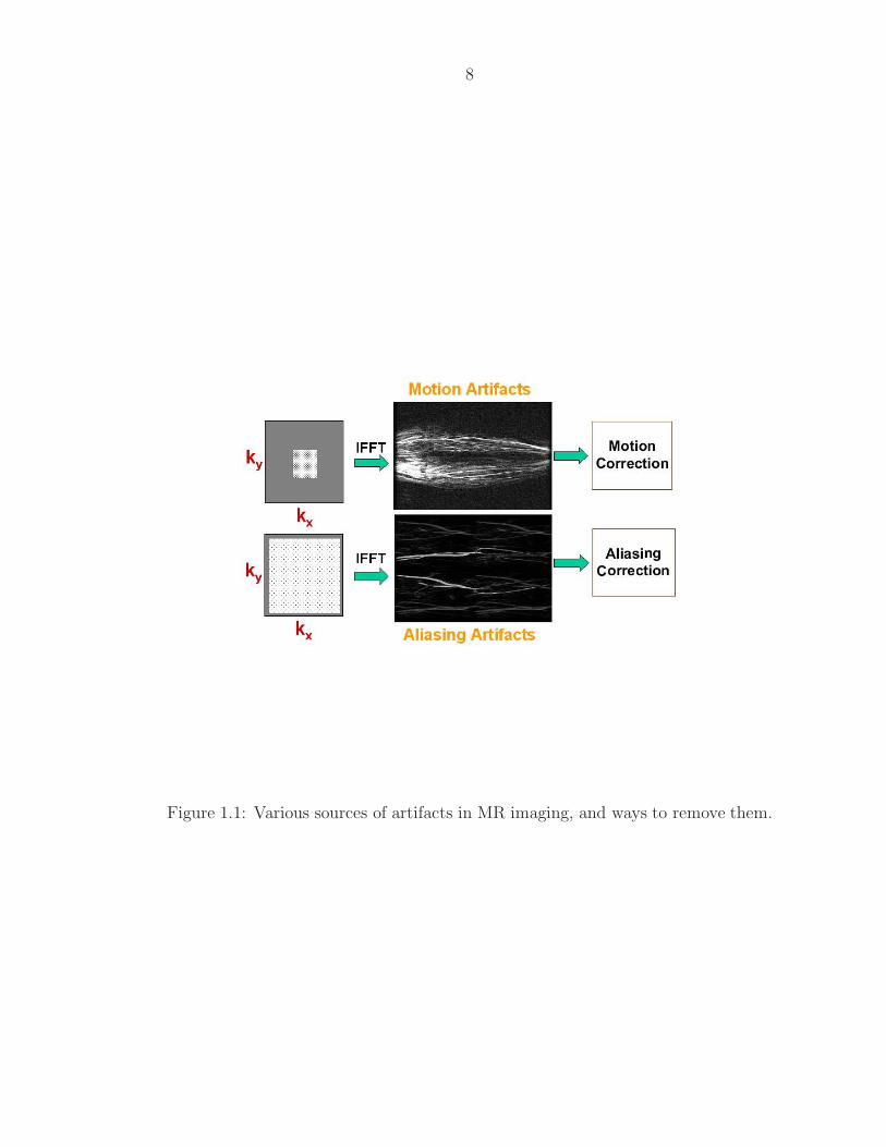
a favourable direction. This point is pictorially represented by figure 1.1.

The images shown in the figure are of the vasculature of the trifurcation re-

gion. As indicated, short scan times cause aliasing artifacts, whereas long scan

times cause motion artifacts. The figure also suggests two possible approaches for

removing these problems: one can either de-aliase the images (parallel imaging),

or remove artifacts caused by long scans (motion correction). The former approach

is useful at the acquisition and reconstruction stages, while the latter is basically

a retrospective post-processing approach. Either approach achieves a favourable

8

Figure 1.1: Various sources of artifacts in MR imaging, and ways to remove them.

9

shift in the tradeoff point, albeit in completely different but complementary ways.

In the following chapters we will present three different algorithmic approaches

to improve MR acquisition, reconstruction and post-processing. These approaches

seem, at first sight, to be rather disparate, intended for different applications. How-

ever, each approach essentially exploits information redundancy to obtain better

image quality for a given scan time, or reduces scan time for constant quality.

The first technique is on correction of motion artifacts in MR Angiography data.

The second technique provides a new reconstruction algorithm for parallel imaging

under a more realistic noise model than what is assumed in conventional methods

like SENSE. The third technique performs fast, stable reconstruction of parallel

data using an edge-preserving Markov Random Field (MRF) - based Bayesian es-

timation algorithm. Each of these methods is a “standalone” application, meaning

they can be used independently or in combination with each other. But as we have

emphasized above, they must be viewed as attempting to solve the same funda-

mental problem: how to use information redundancy to get better quality images

for a certain scan time, and vice versa. We now present a unified description which

connects all these approaches through a linear systems viewpoint.

1.3.1 A linear systems approach to MR imaging

Problems in MR imaging, whether for multiple coils or single coil, can in general

be viewed as the following linear system

y = Ex + n, (1.1)

where x is the desired image to be estimated, y represents observed data, n is addi-

tive instrumentation noise and E is the system matrix. The quantities concerned

10

are defined either in k-space or image space. We will describe in chapter 2 the

detailed derivation of this model for single and multiple receiver coils. When using

a single coil no speed-up is possible, and the data needs to be acquired densely in

k-space. As we have pointed out, this lengthens the scan time, which can limit

image quality due to motion artifacts. So the first and most obvious algorith-

mic challenge is to perform some kind of retrospective motion correction on the

fully sampled Fourier-space data. A new algorithm performing this task, based on

convex projections and called POCS motion correction, is described in chapter 3.

Since the motion problem can be quite difficult to remove in general, it is usually

desirable to reduce its likelihood by accelerating the acquisition process via parallel

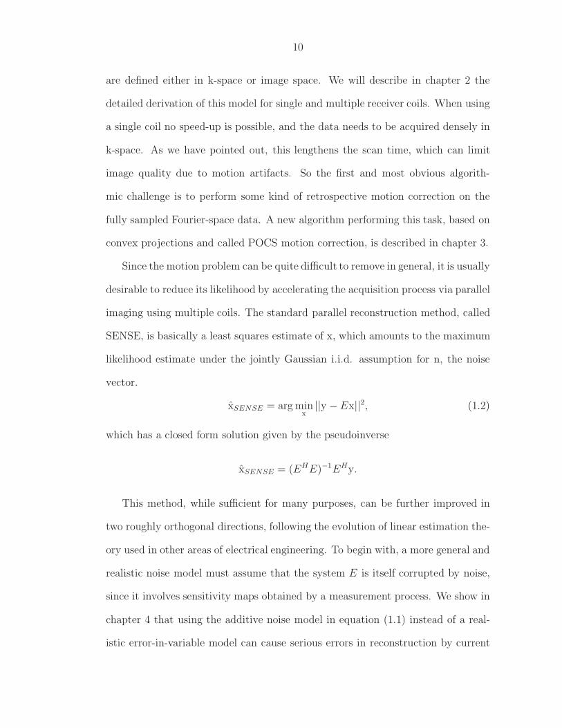
imaging using multiple coils. The standard parallel reconstruction method, called

SENSE, is basically a least squares estimate of x, which amounts to the maximum

likelihood estimate under the jointly Gaussian i.i.d. assumption for n, the noise

vector.

xSENSE = arg minx

||y −Ex||2, (1.2)

which has a closed form solution given by the pseudoinverse

xSENSE = (EHE)−1EHy.

This method, while sufficient for many purposes, can be further improved in

two roughly orthogonal directions, following the evolution of linear estimation the-

ory used in other areas of electrical engineering. To begin with, a more general and

realistic noise model must assume that the system E is itself corrupted by noise,

since it involves sensitivity maps obtained by a measurement process. We show in

chapter 4 that using the additive noise model in equation (1.1) instead of a real-

istic error-in-variable model can cause serious errors in reconstruction by current

11

methods. Methods such as SENSE assume that the coil outputs contain noise, but

that the sensitivity maps are noiseless. In practice, however sensitivity maps are

subject to a wide variety of errors, and we must consider a new generalized noise

model

y = (E + E)x + n, (1.3)

where we have now introduced an error term in the system matrix E, caused

by sensitivity measurement errors. The exact form of E and the ways to solve

systems of the above kind constitute major sections of chapter 4, but a brief outline

is given here. At first glance, sensitivity noise appears to result in an errors-in-

variables problem of the kind in equation (1.3) that is typically solved using Total

Least Squares (TLS) [GL96]. However, existing TLS algorithms are inappropriate

for the specific type of block structure that arises in parallel imaging. We have

taken a maximum likelihood approach to the problem of parallel imaging in the

presence of independent Gaussian sensitivity noise. This results in a non-quadratic

multivariate optimization problem in chapter 4, which also describes a fast and

efficient algorithm for implementing it.

Another way to extend the standard SENSE reconstruction is to exploit prior

information about the desired image. Indeed, for any given noise model, a Bayesian

estimate is likely to provide significant improvement over SENSE, which is essen-

tially a maximum likelihood method. Most imaging situations allow the estimation

of some useful a priori information about the image to be obtained. One of the

most widely used methods is the Wiener estimate, which is a linear estimator

satisfying the maximum a posteriori (MAP) criterion:

xMAP = arg maxx

Pr(y|x) · Pr(x) (1.4)

It is well-known [Kay93] (chapter 12) that if the additive noise vector n is

12

Gaussian distributed with covariance matrix Rn, and the desired signal x is also

Gaussian distributed with covariance Rx, then the Wiener estimate

xwiener = arg minx

(y − Ex)HRn(y − Ex) + xHRxx, (1.5)

is the optimal estimator, and has a closed form shown below:

xwiener = RxEH(ERxE

H + Rn)−1y. (1.6)

The Wiener estimate for parallel MR reconstruction of MR angiography data

looks very promising compared to standard SENSE. However, the prior parameters,

namely Rn and Rx must be deduced from incompletely sampled data, and therefore

this method is appropriate for dynamic sequences like MRA, where a large number

of frames are available.

For single-frame acquisitions, the Wiener method may not work very well. Fur-

thermore, the Gaussian assumption about MR data is frequently inappropriate in

real imaging situations. This brings us to general Bayesian estimation techniques.

The use of a priori information in a Bayesian context has led to substantial perfor-

mance gains in many areas of engineering, like signal/image denoising and restora-

tion, image deblurring, radar processing, multiuser detection in cellular systems,

etc. We posit that a Bayesian approach can similarly impact the quality of MR im-

age reconstruction. In particular, Bayesian methods relying upon Markov Random

Fields (MRFs) have become very popular in recent work in multi-dimensional in-

verse problems, for many reasons. Many multi-dimensional signals displaying local

(e.g. spatial) correlation seem to be most naturally expressed in terms of MRFs.

Many forms of distribution functions over MRFs, like Gaussian or Gibbsian, have

been proposed to model real life images, videos and medical data. One of the

major properties of non-Gaussian distributions like Gibbsian is that they are more

13

robust to outliers, and result in less smearing of important image features like

edges. A large number of papers have proposed these general signal models for

images, both consumer as well as medical [Li95]. For a general linear system as in

equation (1.1), the MRF-based Bayesian methods seek an estimate of

xMRF = arg minx

||y −Ex||2 + GMRF (x), (1.7)

where GMRF (x) is the a priori term. We use the class of discontinuity-preserving

Gibbsian distribution given by

GMRF (x) =∑

(p,q)∈NV (xp, xq). (1.8)

The neighborhood system N consists of pairs of adjacent pixels, usually the 4-

connected neighbors. The smoothness cost V (l, l′) gives the cost to assign l and l′

to neighboring pixels. Typically the smoothness cost has a discontinuity-preserving

form such as V (l, l′) = min(|l − l′|, K) for some metric |·| and constant K. Such a

smoothness term incorporates discontinuity-preserving priors, which can be justi-

fied in terms of Markov Random Fields [Li95].

Unfortunately, while such models are relatively easy to formulate and under-

stand, the optimization problem associated with them is extremely challenging

from a computational point of view. This is because the associated energy func-

tion is highly non-convex, and can be expected to contain numerous local minima.

Traditional multivariate continuous optimization methods fare rather poorly in

this environment, displaying slow convergence and getting trapped in poor local

minima.

We propose a graph cut-based method to perform fast Bayesian estimation

of x under a Gaussian or Gibbsian distribution defined on a Markov Random

Field. Graph cuts have been used in recent year with spectacular effect on the

14

problem of stereo vision, which is a non-linear inverse problem where the underlying

image is assumed to have a Gibbs distribution over an MRF. Unfortunately this

body of work cannot be easily extended to the case of general linear inversion. In

chapter 5 we develop a new graph cut algorithm which works on general linear

inverse problems, provided the system matrix has non-negative entries. The MR

reconstruction problem with Cartesian sampling falls under this category, as does

general image restoration and deblurring. We provide results of our method on

each of these applications.

1.3.2 A summary of contributions

We provide here a brief overview of each technique developed and described in this

thesis.

1. Correction of motion artifacts in MRA: Chapter 3 presents an automatic

method to remove motion artifacts via a novel application of convex pro-

jections. High-pass phase filtering is combined with convex projections in

Fourier-space and image-space successively to remove motion artifacts. The

method effectively removes motion artifacts without degrading vascular in-

formation. In effect, the method seeks to exploit temporal redundancy to

remove motion artifacts.

2. A Maximum likelihood approach to parallel imaging with sensitivity noise:

This work, presented in Chapter 4, develops a maximum likelihood approach

to solving MR reconstruction problems of the kind shown in equation (1.3),

by allowing for errors in sensitivity maps. This looks at first glance to be a

classic error-in-variables problem usually solved by total least squares (TLS)

15

methods. However, we show that TLS algorithms are inappropriate for the

specific type of block structure that arises in parallel imaging. We start

from first principles and derive a simple energy cost minimization, and show

that this results in a quasi-quadratic objective function. We discuss efficient

algorithms for energy minimization under Cartesian sampling schemes. This

method effectively exploits receiver redundancy for resolution and scan time

improvements.

3. Bayesian MR reconstruction from multiple coil data: In Chapter 5 we present

a general and powerful approach of using graph cuts to solve Bayesian re-

construction problems under MRF-based priors. MRF based approaches

are popular due to locally adaptive reconstruction and their edge-preserving

nature. We show however that the resulting reconstruction problem is com-

putationally prohibitive, and suggest a new graph cut energy minimization

approach. However, existing graph cut methods cannot be used for this prob-

lem, and we develop a modified algorithm. Our technique is a natural and

powerful way to exploit spatial redundancy present in MR data.

4. Using Graph Cut Techniques for Other Linear Inversion Problems: We show

further that apart from MR reconstruction, many pixel labeling problems in

early vision, such as image restoration, motion deblurring, etc can benefit

from the graph cut approach. In fact most linear multi-dimensional systems

involving non-negative matrix elements can be solved within a Bayesian MRF

framework using small modifications of our algorithm. We present results on

image deblurring and motion deblurring.

16

We point out that the first technique is geared specifically towards MR angiog-

raphy, while the other techniques are more generally applicable. It is noteworthy

however, that the techniques contained in this thesis are especially suited for MRA,

an important and life-saving procedure. Taken together, these techniques hold the

promise of significantly improving the state of the art in MRA. This is owing to

the fact that MRA suffers more than most other modalities from time, artifact,

noise and resolution constraints. A combination of motion correction, realistic

noise models, and MRF-based Bayesian reconstruction can be easily developed for

MRA, and holds great potential in this area.

Chapter 2

Introduction to MR Imaging

This chapter provides a short description of MR imaging principles and techniques.

The chapter is divided into two parts. The first part, §2.1, contains a brief overview

of the fundamentals of MR imaging, including the underlying physics. The second

part, §2.2, describes the imaging process in MR, both for single as well as multiple

receivers. The second case in particular is a relatively new development in MR,

and is popularly referred to as Parallel Imaging. We discuss this case in some

detail, since it forms the basis of our work in accelerated acquisition techniques,

described in chapters 4 and 5.

2.1 A brief introduction to MR imaging

Differing contrast response of different tissues in the body is the basis for MR imag-

ing. In contrast to other technologies like CT, the contrast behaviour of these tissue

regions can be altered drastically by using different acquisition techniques (called

pulse sequences). This is one of the main reasons for the power and popularity of

MRI. The MR image is produced by mapping the magnetization properties of pro-

tons within tissues. The mechanics of MRI are very complex, and we will provide

a very brief overview of the same. For a simple, readable and non-mathematical

introduction to MR physics and engineering, we refer the reader to the excellent

monograph by McRobbie et al.[DEMM03]. A more comprehensive and technical

treatment, from a signal processing point of view, may be found in [LL99].

During scanning, the MR scanner creates a magnetic field B0 along which the

17

18

spinning protons align themselves, a process called magnetization. The proton

spins in turn precess about th external field at the frequency, called Larmor fre-

quency, which is proportional to the external field:

ν = γB0.

The strength of this magnetization is proportional to the density of proton dipoles

within tissue regions, referred to as proton density or PD. To acquire data, an

additional radio-frequency (RF) pulse in the transverse direction is applied, which

tips the spinning dipoles into the transverse plane. During the period these dipoles

re-align themselves back to B0, they emit RF signals which are picked up by

receiver coils placed around the tissue. By a carefully orchestrated sequence of

field gradients and other hardware, the resulting signal is frequency encoded, i.e.

the frequency of the RF signal emitted by tissue protons varies according to their

spatial position. It turns out that this frequency encoding is exactly identical to

the well-known Fourier Transform. Hence the data points acquired by the receiver

coils map directly onto the space of Fourier coefficients of image dimensions. For a

three-dimensional image, the raw data get mapped to the (kx, ky, kz)-space, usually

referred to within the MR community as k-space.

To demonstrate frequency encoding, let us consider an experiment, where we

are interested in imaging a one-dimensional image, along the x-direction. Suppose

the external B0 field is varied linearly along x, as per B = B0 + xGx. Then the

frequency of the signal generated by the magnetization at x will be given by

ν(x) = γ(B0 + xGx) = ν0 + γGxx.

In other words, the frequency content of the received signal is a direct mapping

of the one-dimensional image! The overall received signal due to the spin density

19

I(x) (corresponding to the tissue under investigation) for any given gradient value

Gx is given by

y(t) = constant ·∫

I(x) exp(−iγGxxt)dx.

Now Gx is time-dependent in general, and we introduce kx =∫ t

0γGx(τ )τdτ , and

obtain

y(kx) = constant ·∫

I(x) exp(−ikxx)dx,

which is nothing but the Fourier transform of I(x)! Therefore, we can recover the

”image” I(x) by simply performing the inverse Fourier transform of y(kx). The

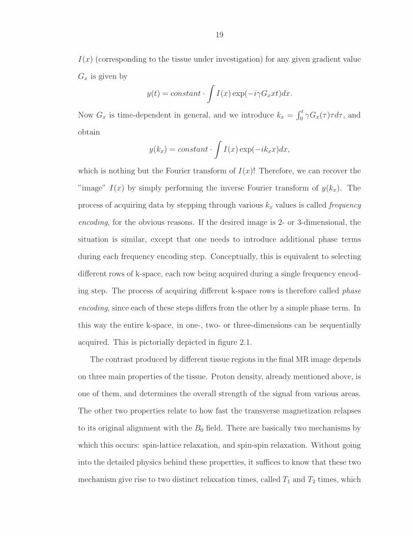
process of acquiring data by stepping through various kx values is called frequency

encoding, for the obvious reasons. If the desired image is 2- or 3-dimensional, the

situation is similar, except that one needs to introduce additional phase terms

during each frequency encoding step. Conceptually, this is equivalent to selecting

different rows of k-space, each row being acquired during a single frequency encod-

ing step. The process of acquiring different k-space rows is therefore called phase

encoding, since each of these steps differs from the other by a simple phase term. In

this way the entire k-space, in one-, two- or three-dimensions can be sequentially

acquired. This is pictorially depicted in figure 2.1.

The contrast produced by different tissue regions in the final MR image depends

on three main properties of the tissue. Proton density, already mentioned above, is

one of them, and determines the overall strength of the signal from various areas.

The other two properties relate to how fast the transverse magnetization relapses

to its original alignment with the B0 field. There are basically two mechanisms by

which this occurs: spin-lattice relaxation, and spin-spin relaxation. Without going

into the detailed physics behind these properties, it suffices to know that these two

mechanism give rise to two distinct relaxation times, called T1 and T2 times, which

20

Figure 2.1: Schematic description of frequency- and phase-encoding steps used to

acquire k-space data.

are intrinsic to the tissue in question. By carefully choosing the acquisition pulse

sequence, the MR technologist can obtain images which are weighted according

to any one of these three tissue properties. The resulting images are then said

to be either T1-weighted, T2-weighted, or PD-weighted. Since different tissues in

the body have different values of these parameters, a radiologist is usually able to

exert great control over the contrast properties of the region being imaged.

2.1.1 Sampling k-space along trajectories

As described above, MR data is acquired in the Fourier- or k-space via a number

of phase-encoding and frequency-encoding steps. We indicated that these steps

are equivalent to acquiring single rows in k-space at a time. But in practice the

data acquired can fall along not just rows, but more general trajectories, although

the pulse sequences for these other trajectory types becomes considerably more

21

Figure 2.2: Popular k-space trajectories.

complex. Some of the most popular trajectory types are listed below, in the

approximate order of popularity. Examples of these different trajectories are shown

in figure 2.2.

1. Cartesian: Linear trajectories with regularly spaced sample points - the

standard row-by-row order mentioned above. Figure 2.1 shows the stan-

dard Cartesian technique. Another Cartesian sampling method called EPI

is shown in figure 2.2.

2. Spiral: Spiral trajectories with several spiral “leaves” oriented regularly around

the circle.

3. Radial: Radial trajectories with regularly spaced sample points along each

radial “spoke”.

Due to the mechanics of the gradient switching and RF pulse sequences used,

it turns out that densely-spaced samples along these trajectories can be acquired

relatively fast. However, the process of going from one trajectory to the next in

k-space requires some time-delay which is dependent on tissue properties like T1,

22

T2 and PD, as well as the particular pulse sequence being used. This time delay is

usually of a magnitude which makes the overall acquisition time of the entire image

quite large, of the order of several seconds for a single 2D image. Thus MRI suffers

from a much slower scanning process than other technologies like CT or PET. Since

the number of trajectories in any given k-space data set must be large enough for

dense sample packing, there is usually a lower limit for any particular situation

below which the scan time cannot be reduced without causing aliasing artifacts

(described in the next section). Some exciting new methods have recently been

discovered that promise to speed up the scanning process, and will be described

in detail in §2.2 below. We note that speedup obtained by these methods is not

due to a basic improvement in MR hardware or pulse sequence design, but rather

in the process of reconstruction.

2.2 Accelerated scanning using parallel imaging

As mentioned in the previous chapter, one of the major disadvantages of using

MRI is its slow scan time. More specifically, there is more or less a linear depen-

dence of imaging resolution with scan time. For certain clinical applications like

cardiac imaging, this problem has limited the use of MR methods. This is because

we need to scan this region quickly to avoid motion artifacts that may result from

the breathing process. However, a high-resolution scan of the cardiac region is not

possible within such a small duration using current techniques. The development

of new accelerated scanning techniques has therefore resulted in bringing several

new MR application areas within feasibility, that were earlier considered impracti-

cal. In the last few years, several techniques have been developed that use multiple

coils to substantially reduce scan time (and thus motion artifacts) without signif-

23

icant loss of image quality. The best-known such technique is SENSE [PWSB01],

although there are also other methods such as SMASH [MOY+01] and GRAPPA

[WND+03]. The basic idea of each of these methods is to speed up the acquisition

by subsampling data in Fourier space, thereby causing aliasing or folding in image

space. The aliasing is removed, and the full-resolution unaliased image recovered,

by the use of multiple receiver coils, in contrast to traditional scanning where a

single receiver coil is used. Although the techniques mentioned above have some

differences in terms of certain specifics, they are all essentially identical from a

high-level viewpoint as described above. These methods have had a significant im-

pact in the medical imaging community; for example, a recent paper [vdBWK+03]

states that “SENSE has opened new horizons in both routine and advanced MR

imaging”. In this thesis we will mainly use the SENSE algorithm when we talk

about parallel imaging, since SENSE is widely recognized as the most general as

well as powerful implementation of parallel imaging concepts [vdBWK+03]. Let

us now describe the method in detail.

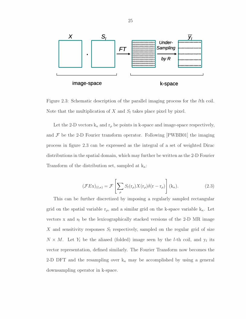
SENSE, like other parallel imaging schemes, uses multiple coils to subsample in

k-space. Each coil also has a sensitivity map, which encodes the different responses

of each coil over the imaging volume. These sensitivity maps are typically obtained

by scanning with a phantom. The outputs of each coil can be combined with the

sensitivity maps to reconstruct a full, unaliased image. The MR parallel imaging

process is most naturally expressed in k-space as a linear system of the form

y = Ex + n, (2.1)

where y contains the (k-space) outputs of the receiver coils, E contains the (k-

space) sensitivity maps, and x is the (k-space) image.1 The reconstruction al-

1See [GBD04] for a study of noise in medical imaging.

24

gorithm used by SENSE assumes that the output of the receiver coils has been

corrupted by noise, represented by the vector n2. A more detailed formalization

of the imaging process will be presented in section 4.1.2. Along with the k-space

input-output model (2.1), we will also use the image-space input-output model:

y = Ex + n, (2.2)

where x, n and y are in the spatial domain. As we will see in section 4.1.2, both

E and E have specific block structures as a result of the imaging process. K-space

noise n is assumed to be Gaussian, independent and identically distributed (i.i.d.).

Then due to the property of the Fourier transform, the image-space noise n is

also i.i.d. Gaussian. The SENSE method takes a least squares approach, which

is natural under these assumptions. Note that the least squares solution is well-

known to be the maximum likelihood estimate [PTVF92, Ch. 15], again assuming

this noise model.

2.2.1 System model

The system matrices E and E represent a concatenation over all coils of the dis-

cretized encoding operator which acts on the input image vector x and k-space

vector x, respectively. The vector x is a discrete representation of the desired MR

image X(rρ), where rρ ∈ Ω is the 2-D spatial vector distributed over the support

Ω of the image, and indexed by ρ, the spatial index. The parallel imaging process

for each coil l can be summarized by figure 2.3, where Sl is the sensitivity map of

the l-th coil, sampled on the same grid as X.

2We will use the notation that x represents a k-space object, while x is animage-space object; we will also denote 1D objects in lower case, and 2D objectsin upper case.

25

X Sl yl

.. FTUnder-

Sampling

by R

image-space k-space

X Sl yl

.. FTUnder-

Sampling

by R

image-space k-space

Figure 2.3: Schematic description of the parallel imaging process for the lth coil.

Note that the multiplication of X and Sl takes place pixel by pixel.

Let the 2-D vectors kκ and rρ be points in k-space and image-space respectively,

and F be the 2-D Fourier transform operator. Following [PWBB01] the imaging

process in figure 2.3 can be expressed as the integral of a set of weighted Dirac

distributions in the spatial domain, which may further be written as the 2-D Fourier

Transform of the distribution set, sampled at kκ:

(FEx)(l,κ) = F[∑

ρ

Sl(rρ)X(rρ)δ(r − rρ)

](kκ). (2.3)

This can be further discretized by imposing a regularly sampled rectangular

grid on the spatial variable rρ, and a similar grid on the k-space variable kκ. Let

vectors x and sl be the lexicographically stacked versions of the 2-D MR image

X and sensitivity responses Sl respectively, sampled on the regular grid of size

N × M . Let Yl be the aliased (folded) image seen by the l-th coil, and yl its

vector representation, defined similarly. The Fourier Transform now becomes the

2-D DFT and the resampling over kκ may be accomplished by using a general

downsampling operator in k-space.

26

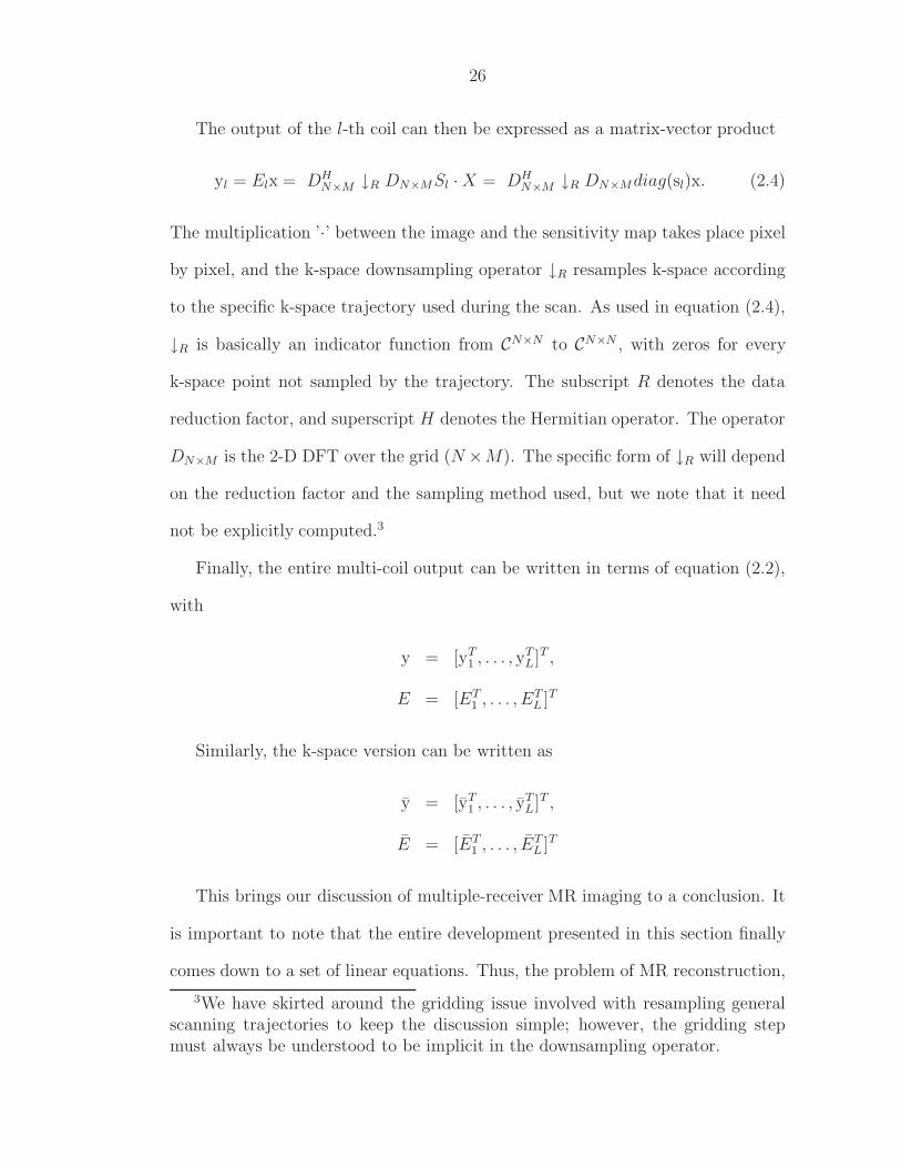
The output of the l-th coil can then be expressed as a matrix-vector product

yl = Elx = DHN×M ↓R DN×MSl · X = DH

N×M ↓R DN×Mdiag(sl)x. (2.4)

The multiplication ’·’ between the image and the sensitivity map takes place pixel

by pixel, and the k-space downsampling operator ↓R resamples k-space according

to the specific k-space trajectory used during the scan. As used in equation (2.4),

↓R is basically an indicator function from CN×N to CN×N , with zeros for every

k-space point not sampled by the trajectory. The subscript R denotes the data

reduction factor, and superscript H denotes the Hermitian operator. The operator

DN×M is the 2-D DFT over the grid (N ×M). The specific form of ↓R will depend

on the reduction factor and the sampling method used, but we note that it need

not be explicitly computed.3

Finally, the entire multi-coil output can be written in terms of equation (2.2),

with

y = [yT1 , . . . , yT

L]T ,

E = [ET1 , . . . , ET

L ]T

Similarly, the k-space version can be written as

y = [yT1 , . . . , yT

L]T ,

E = [ET1 , . . . , ET

L ]T

This brings our discussion of multiple-receiver MR imaging to a conclusion. It

is important to note that the entire development presented in this section finally

comes down to a set of linear equations. Thus, the problem of MR reconstruction,

3We have skirted around the gridding issue involved with resampling generalscanning trajectories to keep the discussion simple; however, the gridding stepmust always be understood to be implicit in the downsampling operator.

27

with either single or multiple coils, is basically one of linear inversion. In the next

three chapters we will describe some new methods of performing this inversion, as

well as some techniques to remove artifacts from already inverted data.

Chapter 3

Motion Correction in Time-Resolved

MR Angiography Using Convex

Projections

Time-resolved 2D Magnetic Resonance Angiography (MRA) is a promising clinical

tool that suffers significantly from motion artifacts. In this chapter we present an

automatic method to remove motion artifacts via a novel application of convex

projections. The method works by exploiting temporal redundancy available in

time-resolved MRA data to remove motion artifacts. We identify a large class

of non-rigid in-plane motions where our method should be effective. High-pass

phase filtering is combined with convex projections in Fourier-space and image-

space successively to remove motion artifacts. The projections are designed to

avoid degrading vasculature information during this process. The algorithm is

stable, and converges quickly, usually within five iterations. Results on a large

set of clinical MRA cases indicate significant improvement in the visual quality of

angiograms. A double-blind evaluation shows that the algorithm produces signifi-

cantly better scores (p = 0.016) when compared to angiograms produced manually

by experienced radiologists.

28

29

3.1 Introduction

Time-resolved 2D Magnetic Resonance Angiography (2D MRA) is a promising

clinical tool for non-invasive diagnosis of vascular diseases [MTJ98]. In 2D MRA a

sequence of 2D MRI images is obtained while a contrast agent is injected. Typically

each image takes approximately 2 seconds to acquire, and the entire sequence lasts

about a minute. Subtraction of pre-contrast images (often called mask images)

from post-contrast (arterial phase) images is then performed to obtain an image of

the vasculature, that is, an angiogram. MRA provides both temporal information

about blood flow as well as anatomic information about the vascular conduit. It

eliminates the risks of iodinated contrast, X-ray radiation and arterial puncture

used with conventional angiography. Instead it utilizes an intravenous injection

of Gadolinium contrast which has an extraordinary safety profile, especially when

compared to iodinated contrast. The MR data can be acquired in just a few

minutes and does not require any of the post-procedural care needed with the

arterial punctures used with conventional angiography. The subtraction of mask

from arterial phase makes the technique very sensitive to Gadolinium so that tiny

doses (e.g. ∼6 ml) can be used.

Patient motion is always a major challenge in MR, but 2D MRA is particularly

susceptible to motion. The action of the contrast agent leads to small changes

changes in intensity, while motion often leads to large intensity changes. Motion

not only reduces the overall image quality, but can also obscure important tem-

poral events like the arrival of contrast agent and the temporal evolution of the

angiogram. As a result, important dynamic data relating to vascular evolution runs

the risk of being completely swamped by even small amounts of patient motion.

Motion of elongated structures (e.g. bones) can create a subtraction artifacts re-

30

sembling arteries. In many cases, the radiologist is forced to discard several frames

with excessive motion artifacts, which can lead to potentially serious gaps in the

temporal MRA record, and may even cause a misdiagnosis.

There has, of course, been a great deal of work on motion correction in MR

(we provide a brief survey in §3.2.2). However, previous work has focused on rigid,

global motion in single-frame MR images. In 2D MRA, however, it is necessary to

handle a much larger variety of motion. Motion in the middle of the acquisition

of a 2D image is particularly challenging, since that is when the low-frequency

components of the image are acquired.

While handling motion in MRA is generally difficult, in 2D MRA the task is

simplified by the availability of a sequence of images. Although patient motion

is difficult to model, it is typically of fairly limited duration, and can potentially

be overcome by exploiting the wealth of temporal data that 2D MRA provides.

To this end, we present an iterative algorithm based on the widely used method

called Projections Onto Convex Sets, or POCS (§3.2 contains a brief review of pre-

vious applications of POCS). By applying POCS in a novel manner, our algorithm

corrects for motion without degrading radiologically important temporal events.

Our POCS-based method iteratively applies successive constraints to the cor-

rupted frame, making it more similar to an artifact-free reference frame that is

computed from other input frames. The constraints applied consist of four projec-

tions, two defined in image space, and two in Fourier space (usually called k-space

in MR). These projections, described in §3.3, were designed specifically to prevent

obliteration of vascular features, and to ensure stability and convergence of the

POCS algorithm. We have identified a large class of non-rigid in-plane motions

(defined formally in §3.4) where our method should be effective. Articulated limb

31

motion (bending, shifting) falls under this category. The results of our algorithm

have been evaluated on a large set of clinical MRA cases collected over several

months. Significant improvement in visual quality was reported in several cases

exhibiting motion. A double-blind evaluation on 47 cases returned a p-value of

0.0162 on a two-tailed t-test, clearly indicating significant overall improvement

over manually obtained angiograms.

The rest of this chapter is organized as follows. Section 3.2 presents an overview

of MRA motion correction and related work, as well as a highlighting some assump-

tions made in our approach. Section 3.3 describes the POCS motion correction

algorithm in detail, with sub-sections (A) to (D) devoted to each of its four convex

projections. Of particular note is a new high-pass phase filtering operation to sup-

press non-global translational motion, described in §3.3.2. While the other three

projections are easy to understand, our high-pass phase filter requires additional

analysis, which is provided in §3.4. We give a detailed spectral analysis which

suggests that a broad class of in-plane motions will result in low-frequency (band-

limited) phase artifacts; such artifacts can be reduced by our high-pass phase filter.

In §3.5 experimental results are presented for simulations as well as real clinical

cases. The data reported by a double-blind evaluation of our technique is also

included, and helps validate the new technique.

3.2 Overview of Proposed Method

Our automatic technique begins by identifying mask and arterial phase MRA frame

using the algorithm described in [KZ03]. Motion-corrupted frames are corrected

using the POCS algorithm, as shown in Figure 3.1. The process repeats for each

corrupted frame in the sequence. The POCS algorithm assumes that an uncor-

32

. . . . . . . . .

IkIk-1Ik-n

I (k)ref POCS Ikcorr

frame number

ref

Figure 3.1: Overview of Motion Correction on MRA: the kth frame has motion

artifacts, which are removed by the POCS algorithm by using the reference frame

rupted reference image can be obtained from the reference set, the set of nref

frames preceding the corrupted frame, as indicated in the figure. A median or

mean operation on the reference set is usually sufficient. The median is preferred

as a more robust average, since it can remove the effect of outliers caused by mo-

tion in the reference set. We note that the implied “direction” in the sequence

(left to right) is entirely arbitrary — the sequence could be processed from right

to left, or different parts of the sequence could be processed in different orders.

The choice of nref is dependent on the levels of motion; it should be the smallest

number sufficient to effectively mitigate motion noise in the reference set. We

also experimented with more elaborate reference sets, for example sets striding

either side of the frame in question, but the improvement was insignificant. Other

enhancements like iterating the process over the entire sequence several times was

found to yield little additional performance, on the other hand suffering from

greater risk of obliterating important radiological features.

33

3.2.1 Assumptions

The most important assumption in our method is that it is possible to obtain a

good reference image. Note that, as described above, the reference image is not a

single image in the input, but rather is computed from nref input images. While

our assumption fails if there is excessive motion in all or a majority of frames, such

situations appear to be infrequent. Isolated instances of motion in the reference set

will be ignored by the median operation. In cases with pervasive motion, taking

the median over the reference set should produce a reference image with low levels

of motion noise.

We also make a few assumptions in our individual projections. The first two

projections, which take place in k-space, assume that the changes in k-space due

to the contrast agent can be distinguished from the changes due to motion. The

first projection (P1 in §3.3) assumes that the vasculature is concentrated in image

space, and hence distributed in k-space. The second projection (P2) can soundly

distinguish the action of the contrast agent, provided the motion arises a large

class of in-plane motions. The image space projections (described under P3 and

P4 in §3.3) estimate the portions of the image that are parenchyma or background

(air). The estimate is designed to be conservative, and assumes that the image

does not have a large amount of overall motion.

3.2.2 Related Work

Several motion correction techniques have been proposed earlier [ea96], [EK02] to

correct for limited rigid, global motion in single-frame MR images, typically using

subspace analysis. Navigator-based correction of rigid translation motion artifacts

has also been proposed, with some success in removing non-rigid motion [MP03].

34

Some correction techniques have also been proposed to correct for global, rigid

in-plane translation in MR temporal sequences [Hog03]. However, this method

only works for rigid, global translation, and assumes that the motion is basically

a step function in time, and occurs between frame acquisitions rather than during

a frame acquisition. These methods are perhaps best suited for brain imaging

since the motion in that case is expected to be rigid. However, none of these tech-

niques are suitable for 2D MRA, because arbitrary amounts of non-rigid motion,

containing rotations as well as translations, can easily occur in the middle of a

frame acquisition. Furthermore, the motion may be non-global in the sense that

certain portions of the field of view of the region imaged may move, while cer-

tain other portions may not. This is particularly relevant for peripheral 2D MRA,

since limbs may move in rather complex ways. Our technique on the other hand

is geared specifically towards motion correction for 2D MRA.

Another technique for mitigating motion was suggested for PET images [PT97]

using motion information from video cameras. This method may be applied to

MRA, but obviously requires additional sophisticated machinery, and tends to be

sensitive to the motion tracking algorithm used. Cardiac gating using EEG has

also been used extensively for peripheral MRA [GWB86], but apart from requiring

additional hardware, its utility in removing patient limb movement is questionable.

A comprehensive survey of correction methods for peripheral DSA is contained

in [MNV99]. While most of these methods are specific to DSA and not readily

applicable to MRA, retrospective methods proposed by the authors are of interest

here. These methods rely on the template matching of moving regions in the

image by using similarity measures bases on cross-correlation and robust measures

of difference. While such techniques are possible for MRA, their utility is much

35

reduced due to the fact that MR images are acquired in k-space. Indeed, the phase

artifacts caused by motion occurring in the middle of k-space acquisition cannot

be removed by purely image-domain methods like template matching. Our POCS

method on the other hand does not suffer from these problems.

POCS methods have been widely used in signal and image processing to per-

form band-limited interpolation and extrapolation [Fer94], image restoration [RA98],

and in optics for non-coherent phase correction, where it is called the Gerchberg-

Papoulis algorithm. These methods have recently been employed with some success

in Partial Fourier MR techniques [OFS88], [XH01]. The success of POCS in so

many different applications stems from the fact that it is a conceptually simple

but powerful way to exploit a-priori constraints and properties that one believes

the solution to possess. A common theme to all these algorithms is that they

try to retrieve missing data from incompletely known data. In particular, Partial

Fourier techniques use POCS to fill-in values for the entire k-space given partial

k-space data covering the central k-space region. The POCS method proposed in

the current work is different from the above POCS applications in the sense that

we do not attempt to retrieve missing data, but to correct corrupted data.

An earlier automatic technique to create angiograms from MRA sequences was

developed by Kim et al. [KPZ+02]. The authors obtain the best angiogram by

evaluating a quality metric, first separating pre- and post-contrast frames. Their

method also identifies motion corrupted frames. Individual frames are not cor-

rected, but if they contain sufficient motion they are not used for subtraction. As

a result, in image sequences with a lot of motion their method can miss impor-

tant events. This algorithm, however, performs a number of useful tasks (such

as detecting contrast agent arrival), and as a result is used as part of the current

36

work.

3.3 POCS Based Motion Correction

POCS motion suppression relies upon projections defined on convex constraint sets.

A set C is said to be convex if and only if for any two members a, b ∈ C a binary

mixture c = αa + (1 − α)b, 0 ≤ α ≤ 1 also belongs to C . Common examples of

convex sets include the set of numbers bounded from above and/or below, and the

set of vectors with magnitudes bounded from above. Each projection is basically a

way to move an arbitrary point in the solution space to a member of the constraint

set that is “nearest” to it. The constraint sets must be convex in order to guarantee

convergence [GPR67, Opi67].

We have used four projections P1 to P4 defined on convex sets, and described in

sections (A) to (D). Starting from the corrupted image, the projections iteratively

reduce motion artifacts by successively making it more similar to the reference

image. The projections have been carefully designed to suppress arbitrary non-

rigid motion artifacts in a variety of ways without degrading vascular enhancement.

In (A)-(D) below and §3.4.1 we present an analysis to ensure that our projections

satisfy this requirement.

Figure 3.2 summarizes our POCS algorithm, with the projections represented

by labeled boxes.

The output of each projection is given by

Ik = (1 − λk)Ik−1 + (λk)Pk(Ik−1), k = 1 . . . , 4, (3.1)

where 0 < λk < 1 are the relaxation factors used to weight the projections, and

Pk are the projections as shown in figure 3.2. The power of the POCS method

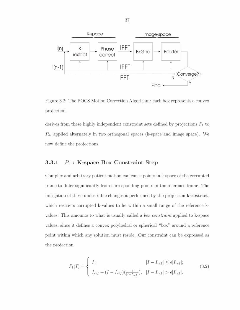
37

I(n)

I(n-1)

IFFT

K-space Image-space

FFT

IFFT

K-

restrictPhase

correctBkGnd Border

N

Y

Converge?

Final

Figure 3.2: The POCS Motion Correction Algorithm: each box represents a convex

projection.

derives from these highly independent constraint sets defined by projections P1 to

P4, applied alternately in two orthogonal spaces (k-space and image space). We

now define the projections.

3.3.1 P1 : K-space Box Constraint Step

Complex and arbitrary patient motion can cause points in k-space of the corrupted

frame to differ significantly from corresponding points in the reference frame. The

mitigation of these undesirable changes is performed by the projection k-restrict,

which restricts corrupted k-values to lie within a small range of the reference k-

values. This amounts to what is usually called a box constraint applied to k-space

values, since it defines a convex polyhedral or spherical “box” around a reference

point within which any solution must reside. Our constraint can be expressed as

the projection

P1(I) =

I, |I − Iref | ≤ ε|Iref |;Iref + (I − Iref )( ε

|I−Iref |), |I − Iref | > ε|Iref |.(3.2)

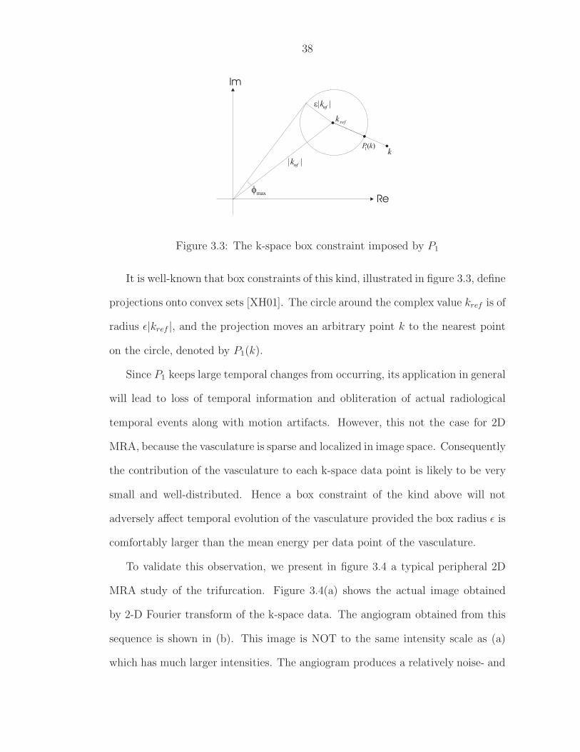
38

Im

Remax

|| refk

|| refk

k)(1 kP

refk

Figure 3.3: The k-space box constraint imposed by P1

It is well-known that box constraints of this kind, illustrated in figure 3.3, define

projections onto convex sets [XH01]. The circle around the complex value kref is of

radius ε|kref |, and the projection moves an arbitrary point k to the nearest point

on the circle, denoted by P1(k).

Since P1 keeps large temporal changes from occurring, its application in general

will lead to loss of temporal information and obliteration of actual radiological

temporal events along with motion artifacts. However, this not the case for 2D

MRA, because the vasculature is sparse and localized in image space. Consequently

the contribution of the vasculature to each k-space data point is likely to be very

small and well-distributed. Hence a box constraint of the kind above will not

adversely affect temporal evolution of the vasculature provided the box radius ε is

comfortably larger than the mean energy per data point of the vasculature.

To validate this observation, we present in figure 3.4 a typical peripheral 2D

MRA study of the trifurcation. Figure 3.4(a) shows the actual image obtained

by 2-D Fourier transform of the k-space data. The angiogram obtained from this

sequence is shown in (b). This image is NOT to the same intensity scale as (a)

which has much larger intensities. The angiogram produces a relatively noise- and

39

background-free rendering of the vasculature. We plot the k-space magnitude of

figure (c) as a function of distance to the center of k-space, in (c). This particular

plot was obtained by averaging the magnitudes of four radial k-space lines — two

vertical and two horizontal. The solid curve is obtained from (b), and the dotted

curve from (c). We note that apart from one or two central pixels containing the

lowest frequencies, the curve of the vasculature maintains almost constant (low)

energy as a function of distance to center. In contrast, the reference data follows

a more pronounced decline in magnitude. To demonstrate that a good choice

of ε will not affect the vasculature data, we plot in (d) the ratio of vasculature

magnitude in k-space to the overall magnitude. Since the ratio is susceptible to

small changes in magnitudes, several radial lines in k-space of several angiograms

had to be averaged to produce the plot. Notice that the highest point of the curve

is lower than 0.25; hence ε > 0.25 will ensure against vascular degradation.

3.3.2 P2 : Phase Correction Step

The second projection, denoted by the box phase-correct, is an interesting phase

filter for correcting translational motion artifacts. It relies on the claim that phase

artifacts due to translation vary smoothly in k-space, whereas the phase informa-

tion due to contrast arrival and vascular evolution is predominantly fast-varying

and erratic. We give experimental evidence for this claim in figure 3.5. While we

cannot prove this claim analytically, we give a theoretical and empirical argument

in favor of it in §3.4, as well as a proof of convexity.

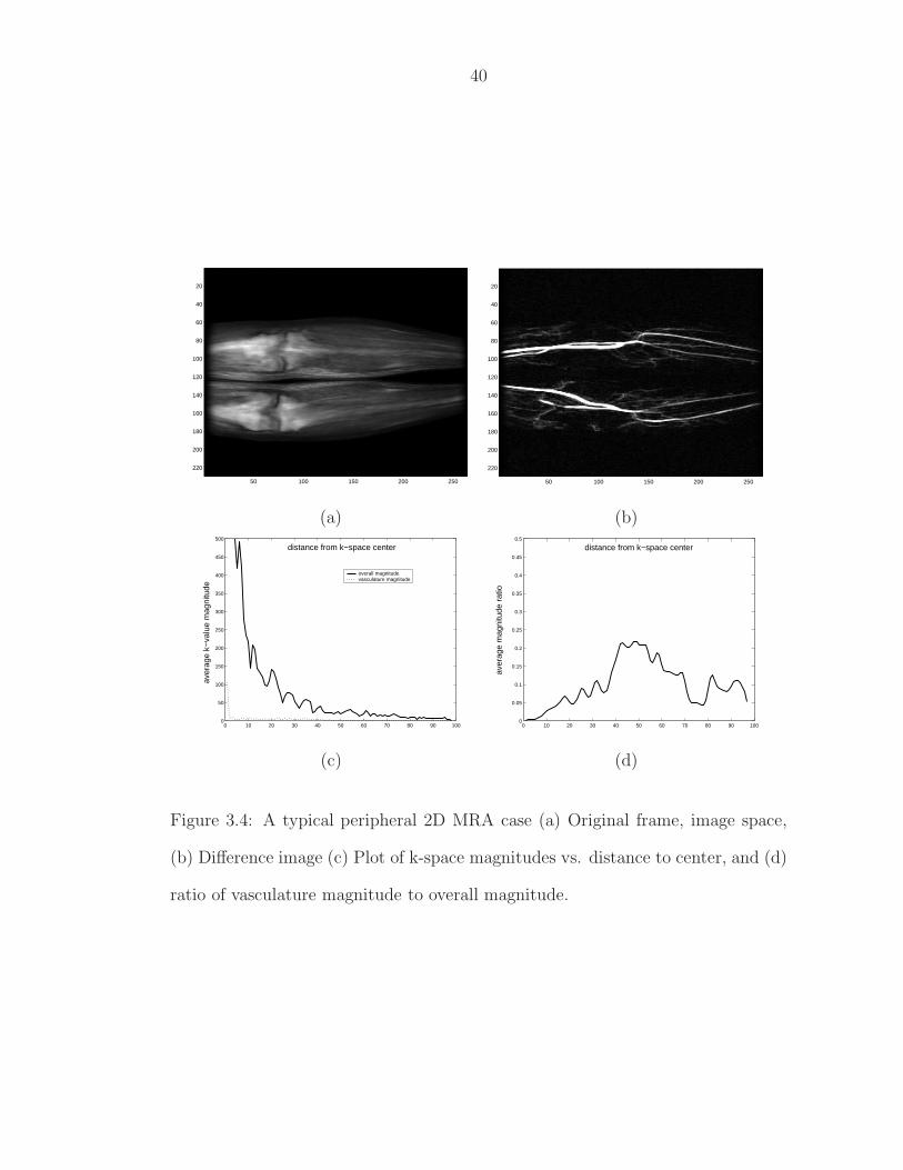
40

50 100 150 200 250

20

40

60

80

100

120

140

160

180

200

220

50 100 150 200 250

20

40

60

80

100

120

140

160

180

200

220

(a) (b)

0 10 20 30 40 50 60 70 80 90 1000

50

100

150

200

250

300

350

400

450

500

distance from k−space center

aver

age

k−va

lue

mag

nitu

de

overall magnitudevasculature magnitude

0 10 20 30 40 50 60 70 80 90 1000

0.05

0.1

0.15

0.2

0.25

0.3

0.35

0.4

0.45

0.5

distance from k−space center

aver

age

mag

nitu

de r

atio

(c) (d)

Figure 3.4: A typical peripheral 2D MRA case (a) Original frame, image space,

(b) Difference image (c) Plot of k-space magnitudes vs. distance to center, and (d)

ratio of vasculature magnitude to overall magnitude.

41

3.3.3 P3 : Parenchyma Correction Step

Projection P3, parenchyma-correct, imposes additional intensity constraints

in image space. It forces the regions of the image reasonably deduced to be

parenchyma (flesh) to be “close” to the corresponding regions of the reference

image via a similar box constraint as in (3.2). Let P be the set of all pixels belong-

ing to regions deduced to be parenchyma. Then for every pixel p in the corrupted

image and the corresponding pixel pref in the reference image

P3(p) =

I(p), p ∈ P ;

I(p), p ∈ P , |I(p) − I(pref )| ≤ η|I(pref )|;I(pref ) + η

I(p)−I(pref)

|I(p)−I(pref)| , p ∈ P |I(p) − I(pref )| > η|I(pref)|.

(3.3)

Again, this is well known to be a projection onto a convex set. Unlike ε, the

box radius η need not be conservative, since we do not expect any useful temporal

information to exist within the parenchyma region. The contrast agent courses

only through the vasculature, and any big or small intensity differences within

parenchyma are likely to be artifacts. The question of deducing the parenchyma

regions from noisy and motion corrupted sequences is quite important. For se-

quences without an enormous amount of motion (§3.2.1) it is possible to obtain

an initial subtracted image of the angiogram from which a reasonable estimate of

the parenchyma regions can be obtained. Fortunately the projection P3 does not

require high accuracy in deducing the parenchyma regions, allowing us to use a

very conservative estimate in order not to introduce subsequent errors.

3.3.4 P4 : Background Forcing Step

The background of an MRA image is the region with no signal, and should ideally

be zero. However, due to instrument noise as well as spurious motion artifacts,

42

this is usually not the case. We therefore impose our final projection P4, BkGnd

in figure 3.2, by deducing the background from the reference image and forcing it

to be zero in the corrupted image. This is clearly a projection onto a convex set,

since any linear combination of two images of zero background produces an image

of zero background. As before, we have used a conservative estimate of background

regions in order not to introduce further errors.

3.4 A High-Pass Phase Filter for Suppression of Transla-

tion Artifacts

In this section we show that phase artifacts caused by general non-global trans-

lation are band-limited to low frequencies through spectral analysis of the phase

under a multi-piece translation model. In figure 3.5 a typical example is shown:

(a) shows a typical spectrum of phase caused by non-global translation (§3.4.4describes how we obtained this plot), and (b) shows a typical spectrum of the

phase caused by the vasculature. This plot was obtained with Burg’s average pe-

riodogram [SM97] from several rows of vasculature phase in k-space. The figure

clearly shows that a modest high-pass phase filter effectively suppresses translation

artifacts. Our filter has an impulse response h = [−0.2,−0.6, 1,−0.6,−0.2], and

the frequency response shown in figure 3.6.

The filter is one-dimensional because we chose to filter only in the Frequency

Encode (FE) direction [MTJ98]. In MRI, it is usually assumed that a single scan

line in the FE direction is sufficiently quick to not suffer from phase distortions like

(3.5) due to patient motion [EK02]. Thus all motion effects may be assumed to

occur between FE lines, not within them. Filtering only in the FE direction there-

43

0 0.1 0.2 0.3 0.4 0.5 0.6 0.7 0.8 0.9 10

0.05

0.1

0.15

0.2

0.25

normalized frequency

pow

er s

pect

ral d

ensi

ty

0 0.1 0.2 0.3 0.4 0.5 0.6 0.7 0.8 0.9 10.2

0.3

0.4

0.5

0.6

0.7

0.8

0.9

normalized frequency

Pow

er S

pect

ral D

ensi

ty

(a) (b)

Figure 3.5: Typical power spectra of phase signals in k-space, obtained from the

phase difference between consecutive frames: (a) Non-global translation; (b) phase

due to vasculature, obtained from an artifact-free sequence.

−1 −0.8 −0.6 −0.4 −0.2 0 0.2 0.4 0.6 0.8 10

0.1

0.2

0.3

0.4

0.5

0.6

0.7

0.8

0.9

1

frequency

Figure 3.6: Frequency response of the high-pass phase filter.

44

fore prevents phase distortion in corrupted FE lines from influencing the phase of

adjacent non-corrupted FE lines. In §3.4.1 we prove the convexity of the projection

defined by the phase filter. The remaining sections discuss the spectral properties

of translation phase.

3.4.1 Proof of Convexity of P2

Proving the convexity of P2 is rather complicated since it acts only on the phase,

and is therefore not guaranteed to define a complex projection in CMN , the space

of M ×N complex images. Theorem 1 proves that this operation does in fact ap-

proximate, to arbitrary accuracy, a convex projection by virtue of the construction

of our algorithm.

Theorem 3.1 Let H(φ(kx, ky)) represent the high pass filtering operation on the

phase image φ(kx, ky) performed by the phase correct step. Let L be the comple-

mentary low-pass filter constructed such that LH = 0. Let C be the set of M × N

complex k-space frames of identical magnitude M(kx, ky), kx = 1 . . . M, ky = 1 . . . N

such that C = M(kx, ky)ei(φ0(kx,ky)+φ(kx,ky)) | L(φ(kx, ky)) = 0. We will drop

the indices (kx, ky) henceforth for convenience. Then

1. The phase correction step defines a projection onto C.

2. Set C approximates a convex set over a region of interest R ⊂ C containing

members with phase bounded by φmax: −φmax ≤ φ ≤ φmax. The error of

approximation is proportional to φ2max.

3. The k-space box projection P1 with box radius ε imposes a bound φ2max on the

phase of the intermediate POCS solution at every iteration, with φmax = ε.

45

Proof:

1. For any A = Mei(φ0+φ), A′ = Mei(φ0+H(φ)) ∈ C , since L(H(φ)) = 0. Hence

phase-correct step with phase filter H defines a projection onto C .

2. Let A1 = Mei(φ0+φ1), A2 = M ei(φ0+φ2) be two members of C . We need to

show that A = αA1 + (1 − α)A2 also belongs to C . We have

A = Meiφ0[αei(φ1) + (1 − α)ei(φ2)].

Linearizing the expression within square brackets by the Taylor Series we

obtain

(α + 1− α) + (αφ1 + (1 − α)φ2)− i

2(αφ2

1 + (1− α)φ22) + higher order terms.

The higher order terms can be omitted since they are likely to be extremely

small for small φ1 and φ2. Expanding this in a Taylor Series in (αφ1 + (1 −α)φ2) by completing the square for the second order terms and omitting

higher terms, we get

A1 = Meiφ0ei((αφ1+(1−α)φ2)) + E,

where the error term E is the residue from completing the square. Now it is

clear that A1 belongs to C up to the error term E, since L(αφ1 +(1−α)φ2) =

0.

Furthermore, it is straightforward to show that E = α(1−α)2

(φ1 −φ2)2. Given

that −φmax ≤ φ1, φ2 ≤ φmax, clearly the maximum error occurs for α = 1/2,

φ1 = −φ2 = φmax, and the maximum error is given by Emax = φ2max/2.

3. From figure 3.3, every k-space data point k of every intermediate solution

must reside within the circle of radius ε|kref | in the complex plane, where kref

46

is the corresponding reference point. Then the maximum phase difference

between any two points in that circle is φmax as shown in the figure. Since a

tangent subtends a right angle at the center, we have sin(φmax) = ε. Result

follows from small angle approximation of sines.

3.4.2 Phase Artifacts For a Piece-wise Motion Model

A global translation of (x,y) in the complex image I(x, y), with K(kx, ky) =

F(I(x, y)) being the k-space image, leads to a linear phase term in k-space given

by K ′(kx, ky) = K(kx, ky) exp(ic(xkx +yky)), for some constant c. The Fourier

transform of this phase is obviously band-limited to low frequencies. We provide

evidence in this section that this continues to be the case even for non-global, non-

rigid translations, provided they can be approximated by the multi-piece motion

model

K ′(kx, ky) =N∑

i=1

Ki(kx, ky) exp(ic(xikx + yiky)), (3.4)

where N is the number of image pieces, and each Ki is the transform of an im-

age piece undergoing translation by (xi,yi). Equation (3.4) is reasonable for

arbitrary non-rigid translation for sufficiently large N .

To begin with, we need a formal definition for band-limited images:

Definition: Let Ω(W ) be defined as the set of two-dimensional smoothly-

varying functions φ(kx, ky) ∈ R2 whose Fourier Transforms F(φ) are

band-limited to the low-frequency band [−W, W ] × [−W, W ], with W

being the angular frequency cutoff.

Using expressions for phase spectra we will argue that the following holds:

47

Proposition 1: The phase difference between the corrupted and ref-

erence frame, φ(K ′, K) = φ(K ′) − φ(K) belongs to Ω(W ), i.e., is

band-limited. Consequently, the power spectral density of φ(K ′, K)

is concentrated in the low frequency region [−W, W ]× [−W, W ].

To keep the analysis uncluttered, we only consider the two-piece model

K ′(kx, ky) = K1(kx, ky) exp(iφ1(kx, ky))

+ K2(kx, ky) exp(iφ2(kx, ky)) · exp(ic(xkx + yky)), (3.5)

where φ(·) denotes the phase of a complex quantity, K1 is the stationary compo-

nent, and K2 undergoes translation. However, this does not cause loss of generality

due to the following theorem.

Theorem 3.2 If Proposition 1 holds for the two-piece model (3.5), then it also

holds for the multi-piece model (3.4). That is, the phase difference φ(K ′, K) is

band-limited for (3.4) as well: φ(K ′, K) ∈ Ω(W ).

Proof: Let

Γnm =

n∑i=m

Ki(kx, ky) exp(ic(xikx + yiky))

γnm =

n∑i=m

Ki(kx, ky)

φ(n) = φ(Γn1 + ΓN

n+1) − φ(Γn−11 + ΓN

n ).

From Proposition 1, φ(n) ∈ Ω(W ) ∀n ∈ [1, N ] since the phase difference is

between two signals differing by only a single component Kn which undergoes

translation. By the definition of φ(n), it is easy to show that

N∑i=1

φ(n) = φ(ΓN1 ) − φ(γN

1 ) = φ(K ′, K).

48

Now the set Ω(W ) is obviously closed under addition, i.e. a sum of signals belong-

ing to Ω(W ) also belongs to Ω(W ). Therefore φ(K ′, K) ∈ Ω(W ).

A general expression of the phase shift is derived (equation (3.6)), but explicit

spectral analysis of this expression is difficult. We instead focus on three separate

cases, whereby the moving piece is considered small, large, and equal, respectively,

compared to the non-moving piece. In each case, a spectrum of φ(K ′, K) is

explicitly derived, and found to be band-limited. We also present computed spectra

of intermediate cases to verify that band-limitedness continues to be true across

all scenarios.

3.4.3 Expression For Phase Difference

We wish to obtain expressions for the phase difference φ = φ′ − φ caused by

the two-piece translation model (3.5). We assume that the phase φ(kx, ky) is a

random process uniformly distributed in [−π, π] with a power spectral density

exhibiting 3 dB cutoff at angular frequency W0. This is reasonable given that

phase is frequently modeled as uniform noise, and that it is quite correlated, if

we neglect instrumentation noise. Let δ(kx, ky) = c(xkx + yky) be the phase

term due to translation. Let φ(kx, ky) be the original phase before motion, and

φ′(kx, ky) be the phase after motion. Figure 3.7 depicts the situation for a single

k-space point. Position A is the original k-value, and position B is the k-value

after translation of K2 by (x,y), causing a phase shift δ. The indices (kx, ky)

have been dropped for simplicity. Theorem 3 summarizes and proves our main

result.

Theorem 3.3 Let δ, φ, φ′ and φ be defined as above, and let the phases of

components K1 and K2 prior to translation be φ1 and φ2 respectively. Let α =

49

|K2|/|K| be the ratio of the moving signal strength to the overall signal strength.

Then

φ = arcsin

(α(sin(φ− φ2) + sin(φ2 − φ + δ))√

1 + 4α2 sin2(δ/2) + 4α sin(φ − φ2 − δ/2) sin(δ/2)

), (3.6)

Proof: In figure 3.7 angle ∠AOX is the original phase φ and ∠ACB = δ. We

wish to find ∠AOB = φ, the phase difference. The displacement caused by

motion is given by

AB = 2K2 sin(δ/2), (3.7)

where AB denotes the distance between A and B. Now ∠AOC = q = φ2 − φ and

∠BAC = π/2 − δ/2. Therefore ∠BAO = π/2 − δ/2 − q. Using the Law of Sines

on triangle OBA, we get

sin(φ) =AB

|K ′| sin(∠BAO). (3.8)

Using the Law of Cosines on OBA, we obtain

|K ′| =

√|K|2 + AB

2 − 2KAB cos(∠BAO). (3.9)

Finally, combining (3.7), (3.8) and (3.9) we get after simplification,

sin(φ) =2K2 sin(δ/2) cos(p + δ/2)√

K2 + 4K22 sin2(δ/2) − 4KK2 sin(δ/2) sin(p + δ/2)

. (3.10)

Using α = |K2|/|K| in above, we obtain (3.6). Although φ was derived only

for the first quadrant of the complex plane, and for increasing δ, the same result

obtains in all cases.

The general spectral analysis of (3.6) is difficult. Instead we present results on

important special cases corresponding to |K1| >> |K2|, |K1| = |K2| and |K1| <<

|K2|, covering all scenarios. As in figure 3.7, let p = φ − φ1and q = φ2 − φ. From

the Law of Sines, we get: sin(p)/|K2| = sin(q)/|K1|. Hence for small K1, q is small;

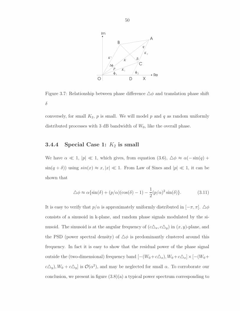
50

O

BA

C

D X

Im

Re

1 2

K'K

1K

2K

p

q

Figure 3.7: Relationship between phase difference φ and translation phase shift

δ

conversely, for small K2, p is small. We will model p and q as random uniformly

distributed processes with 3 dB bandwidth of W0, like the overall phase.

3.4.4 Special Case 1: K2 is small

We have α 1, |p| 1, which gives, from equation (3.6), φ ≈ α(− sin(q) +

sin(q + δ)) using sin(x) ≈ x, |x| 1. From Law of Sines and |p| 1, it can be

shown that

φ ≈ αsin(δ) + (p/α)(cos(δ) − 1) − 1

2(p/α)2 sin(δ). (3.11)

It is easy to verify that p/α is approximately uniformly distributed in [−π, π]. φ

consists of a sinusoid in k-plane, and random phase signals modulated by the si-

nusoid. The sinusoid is at the angular frequency of (cx, cy) in (x, y)-plane, and

the PSD (power spectral density) of φ is predominantly clustered around this

frequency. In fact it is easy to show that the residual power of the phase signal

outside the (two-dimensional) frequency band [−(W0 +cx), W0 +cx]× [−(W0+

cy), W0 + cy] is O(α2), and may be neglected for small α. To corroborate our

conclusion, we present in figure (3.8)(a) a typical power spectrum corresponding to

51

0 0.1 0.2 0.3 0.4 0.5 0.6 0.7 0.8 0.9 10

0.05

0.1

0.15

0.2

0.25

0 0.1 0.2 0.3 0.4 0.5 0.6 0.7 0.8 0.9 10

0.1

0.2

0.3

0.4

0.5

0.6

0.7

0.8

0.9

1

(a) (b)

0 0.1 0.2 0.3 0.4 0.5 0.6 0.7 0.8 0.9 10

0.1

0.2

0.3

0.4

0.5

0.6

0.7

(c)

Figure 3.8: Averaged power spectra of phase signals: (a) Case A, α = |K2|/|K| =

0.2; (b) Case B, α = 0.9; (c) General intermediate case, α = 0.7.

this case. The power spectrum was arrived at for α = 0.2, as follows. Traversing

a typical k-space frame in the frequency-encode direction, we acquired several one

dimensional phase signals. These phase signals were used to model the stochastic

signal p in (3.11). Then we used (3.11) to produce corresponding phase differ-

ence signals. Power spectra of each of these signals was obtained using Welch’s

averaged periodogram method [Wel67]. Figure (3.8)(a) was obtained after aver-

aging these power spectra to produce a relatively noise-free representative power

spectrum. The frequencies are normalized to fall between 0 and 1, with the latter

corresponding to the Nyquist rate. The signal has predominantly low frequencies,

along with a modulation portion centered at the frequency of the phase sinusoid,

at normalized frequency of 0.08, corresponding to 8 percent translation in the field

of view (FOV).

52

3.4.5 Special Case 2: K1 is small

We have α ≈ 1, |q| 1. Let β = |K1|/|K| 1. Equation (3.6) reduces to

φ ≈ arcsin (sin(δ) + β(q/β) cos(δ)(cos(δ) − 1)) , (3.12)

after expanding the denominator of (3.6) as a binomial series and neglecting higher

order terms. As before, q/β is a random process uniformly distributed in [−π, π].

Since the second term is quite small, we can expand the above in a Taylor series

for arcsin(·) about the point sin(δ). We then have, after neglecting higher order

terms,

φ ≈ δ + β(q/β)(cos(δ) − 1). (3.13)

Therefore, the phase difference in this case is basically a linear ramp function,

with a small amount of a modulated random signal of bandwidth W0. The residual

power outside frequency band [−(W0+cx), W0+cx]×[−(W0+cy), W0+cy] is

O(β4), and can be safely neglected. Figure (3.8)(b) presents corroborating evidence

for our conclusion. It was obtained in the same way as described in Case 1, with

α = 0.9, and 8 percent translation.

3.4.6 Special Case 3: K1 and K2 are equal

From figure 3.7 it is easy to show, using basic circle geometry, that

φ = δ/2. (3.14)

This is an interesting result, since it indicates that the phase difference is indepen-

dent of the phase, and is constant! In any case, this is a linear ramp in k-space,

and therefore also lies in the low-frequency region.

53

We have shown that if K2 is much larger, smaller or equal to K1, then the phase

difference in each case is predominantly low-frequency. It is therefore reasonable

to expect that this will continue to be the case for intermediate cases as well.

This is experimentally corroborated by figure (3.8)(c), which shows a typical PSD

corresponding to |K2|/|K| = 0.7.

3.5 Results

3.5.1 Materials and methods

The following data were obtained at 1.5 Tesla with a head coil for signal trans-

mission and reception (LX Horizon, General Electric Medical Systems). Patients

were placed feet-first into the magnet with the legs positioned within the head

coil to image from above the patella down to mid-calf. A sagittal gradient echo

scout sequence was used to position the coronal 2D projection MRA slab so that it

encompassed the entire calf. The 2D projection MRA was performed as a coronal

spoiled gradient echo sequence using the following parameters: TR/TE/ip angle

= 10/2/60 degrees, slab thickness = 7-10 cm, field-of-view = 30cm, matrix =

256x192, bandwidth = 16 kHz. The imaging time was 1.95 seconds per acquisi-

tion, repeated 35 times for a total of 67 seconds. Gadolinium contrast (5-7 ml

at 0.5mol/L) (Magnevist, Berlex Laboratories, Wayne, NJ; Omniscan, Nycomed

Amersham, Princeton, NJ) was injected and flushed with 20 ml saline. The injec-

tion rate was 2.5ml/sec by hand with a SmartSet (TopSpins, Ann Arbor, MI) or

using an automatic injector (Spectris MR Injector, MedRad, Pittsburg, PA). The

injection was initiated simultaneously with image acquisition.

54

3.5.2 In-plane motion in a single frame: Simulation Results

Several experiments were conducted to test the operation of the POCS algorithm

on removing motion artifacts from a single frame within the sequence. For the

purpose of comparison, various kinds of motion were simulated and applied on

an otherwise well-registered and motion-free MRA sequence. The first example

demonstrates POCS results on step-like translational motion as a function of the

PE index, shown in figure 3.9. The translation was non-global - only a part of

the image was caused to move 2 pixels in both the PE and FE directions. In this

example, half of the image undergoes translation after almost half the (Cartesian)

k-space lines have been acquired. This case is exceedingly difficult to correct for

by most current algorithms, since the motion is non-global and has occurred in the

middle of the k-space scan. The results are shown in figure 3.9. The uncorrupted

frame (a) is just prior to the corrupted frame (b) in the MRA sequence. The effect

of the translation is too small to be easily discerned from the actual scans as shown

here, but the resulting difference image, i.e. the angiogram shown in (d) clearly has

significant artifacts when compared to the uncorrupted angiogram shown in (c).

These artifacts make the angiogram quite useless diagnostically. This is a good

example of the extreme sensitivity of 2D MRA to even small amounts of motion.

Part (e) shows the result of the POCS motion correction algorithm applied on the

motion corrupted MRA sequence. Clearly the algorithm has been able to recover

almost all features present in the original uncorrupted angiogram while removing

motion artifacts. The result was obtained after three iterations with relaxation

factor of λ = 0.8.

Figure 3.10 shows another non-global translation example. The amount of

translation was chosen to be large — around a quarter of FOV in the PE direction.

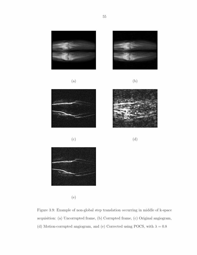
55

(a) (b)

(c) (d)

(e)

Figure 3.9: Example of non-global step translation occurring in middle of k-space

acquisition: (a) Uncorrupted frame, (b) Corrupted frame, (c) Original angiogram,

(d) Motion-corrupted angiogram, and (e) Corrected using POCS, with λ = 0.8

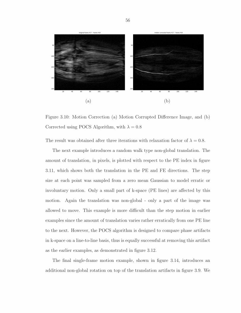
56

original frame #17 − frame #10

20 40 60 80 100 120 140

50

100

150

200

250

motion corrected frame #17 − frame #10

20 40 60 80 100 120 140

50

100

150

200

250

(a) (b)

Figure 3.10: Motion Correction (a) Motion Corrupted Difference Image, and (b)

Corrected using POCS Algorithm, with λ = 0.8

The result was obtained after three iterations with relaxation factor of λ = 0.8.

The next example introduces a random walk type non-global translation. The

amount of translation, in pixels, is plotted with respect to the PE index in figure

3.11, which shows both the translation in the PE and FE directions. The step

size at each point was sampled from a zero mean Gaussian to model erratic or

involuntary motion. Only a small part of k-space (PE lines) are affected by this

motion. Again the translation was non-global - only a part of the image was

allowed to move. This example is more difficult than the step motion in earlier

examples since the amount of translation varies rather erratically from one PE line

to the next. However, the POCS algorithm is designed to compare phase artifacts

in k-space on a line-to-line basis, thus is equally successful at removing this artifact

as the earlier examples, as demonstrated in figure 3.12.

The final single-frame motion example, shown in figure 3.14, introduces an

additional non-global rotation on top of the translation artifacts in figure 3.9. We

57

0 50 100 150 200 250−5

0

5

10

tran

slat

ion

in P

E d

irect

ion

0 50 100 150 200 250−15

−10

−5

0

tran

slat

ion

in F

E d

irect

ion

PE line number

Figure 3.11: Non-global random-walk translation, plotted as a function of the

phase encode index. The top curve shows translation in the PE direction, while

the bottom curve shows translation in FE direction.

58

(a) (b)

(c)

Figure 3.12: Example of non-global random-walk translation occurring in middle

of k-space acquisition: (a) Original angiogram, (b) Motion-corrupted angiogram,

and (c) Corrected using POCS Algorithm, with λ = 0.8

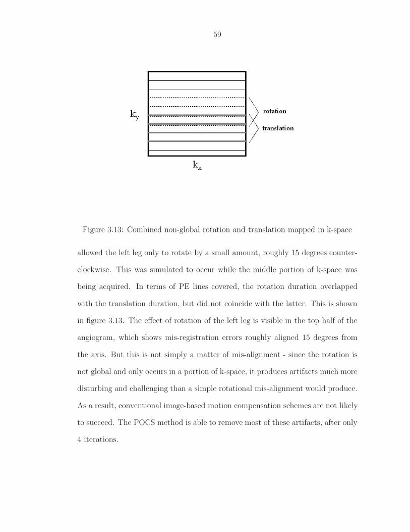
59

Figure 3.13: Combined non-global rotation and translation mapped in k-space

allowed the left leg only to rotate by a small amount, roughly 15 degrees counter-

clockwise. This was simulated to occur while the middle portion of k-space was

being acquired. In terms of PE lines covered, the rotation duration overlapped

with the translation duration, but did not coincide with the latter. This is shown

in figure 3.13. The effect of rotation of the left leg is visible in the top half of the

angiogram, which shows mis-registration errors roughly aligned 15 degrees from

the axis. But this is not simply a matter of mis-alignment - since the rotation is

not global and only occurs in a portion of k-space, it produces artifacts much more

disturbing and challenging than a simple rotational mis-alignment would produce.

As a result, conventional image-based motion compensation schemes are not likely

to succeed. The POCS method is able to remove most of these artifacts, after only

4 iterations.

60

(a) (b)

(c)

Figure 3.14: Non-global rotation as well as translation, both occurring in middle

of k-space acquisition: (a) Original angiogram, (b) Motion-corrupted angiogram,

and (c) Corrected using POCS Algorithm, with λ = 0.8

61

3.5.3 Completely un-supervised clinical MR-DSA: a joint

classification and motion correction algorithm

In clinical practice, after acquisition the MRA sequence is analysed laboriously

by radiologists. Each frame is viewed, and estimates of contrast arrival, arterial

phase (post-contrast), mask phase (pre-contrast) and venous phase are empirically

obtained. Then frames are evaluated according to their quality, and any motion-

corrupted frames are rejected, more or less by trial and error. Then the final

angiogram is obtained by subtracting the set of ”good” mask frames from ”good”

arterial phase frames. A new, automatic MR-DSA algorithm was recently proposed

by Kim et al.[KPZ+02] to automate this time-consuming procedure. In this section

we investigate an extension of this method by incorporating the POCS-based mo-

tion correction algorithm within the automated MR-DSA classification algorithm.

This attempts to remove a major source of error in the work in [KPZ+02], which

was extremely sensitive to motion artifacts. Our unsupervised method performs

motion correction on all frames of all cases. This is obviously both unnecessary

as well as potentially harmful for cases and frames that do not suffer from noise.

However, this approach was necessitated by the fact that the MR-DSA algorithm

did not provide adequate indication of motion corruption. We also wish to demon-

strate that our method is designed to retain radiologically important information.

Clearly, if angiogram quality is degraded if the POCS method is applied on non-

corrupted cases, then that would be a useful piece of information which would help

decide in which situations the method should be applied.

Real clinical cases were obtained from data collected in a recent comparative

study [KPZ+02]. The authors have investigated many peripheral MRA clinical

cases and used a panel of radiologists to identify cases and frames which have mo-

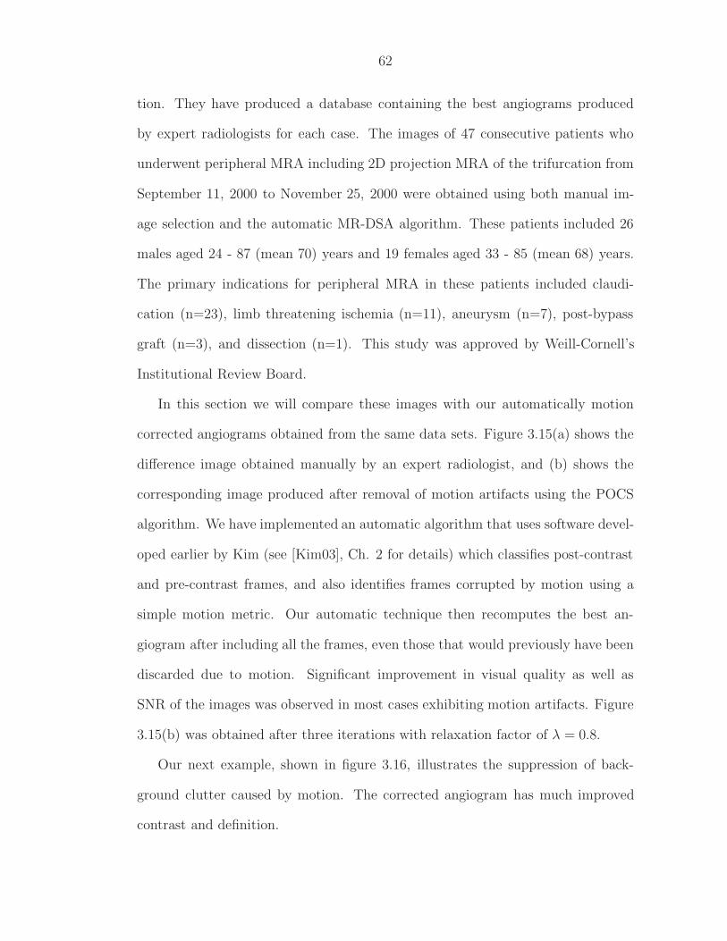
62

tion. They have produced a database containing the best angiograms produced

by expert radiologists for each case. The images of 47 consecutive patients who

underwent peripheral MRA including 2D projection MRA of the trifurcation from

September 11, 2000 to November 25, 2000 were obtained using both manual im-

age selection and the automatic MR-DSA algorithm. These patients included 26

males aged 24 - 87 (mean 70) years and 19 females aged 33 - 85 (mean 68) years.

The primary indications for peripheral MRA in these patients included claudi-

cation (n=23), limb threatening ischemia (n=11), aneurysm (n=7), post-bypass

graft (n=3), and dissection (n=1). This study was approved by Weill-Cornell’s

Institutional Review Board.

In this section we will compare these images with our automatically motion

corrected angiograms obtained from the same data sets. Figure 3.15(a) shows the

difference image obtained manually by an expert radiologist, and (b) shows the

corresponding image produced after removal of motion artifacts using the POCS

algorithm. We have implemented an automatic algorithm that uses software devel-

oped earlier by Kim (see [Kim03], Ch. 2 for details) which classifies post-contrast

and pre-contrast frames, and also identifies frames corrupted by motion using a

simple motion metric. Our automatic technique then recomputes the best an-

giogram after including all the frames, even those that would previously have been

discarded due to motion. Significant improvement in visual quality as well as

SNR of the images was observed in most cases exhibiting motion artifacts. Figure

3.15(b) was obtained after three iterations with relaxation factor of λ = 0.8.

Our next example, shown in figure 3.16, illustrates the suppression of back-

ground clutter caused by motion. The corrected angiogram has much improved

contrast and definition.

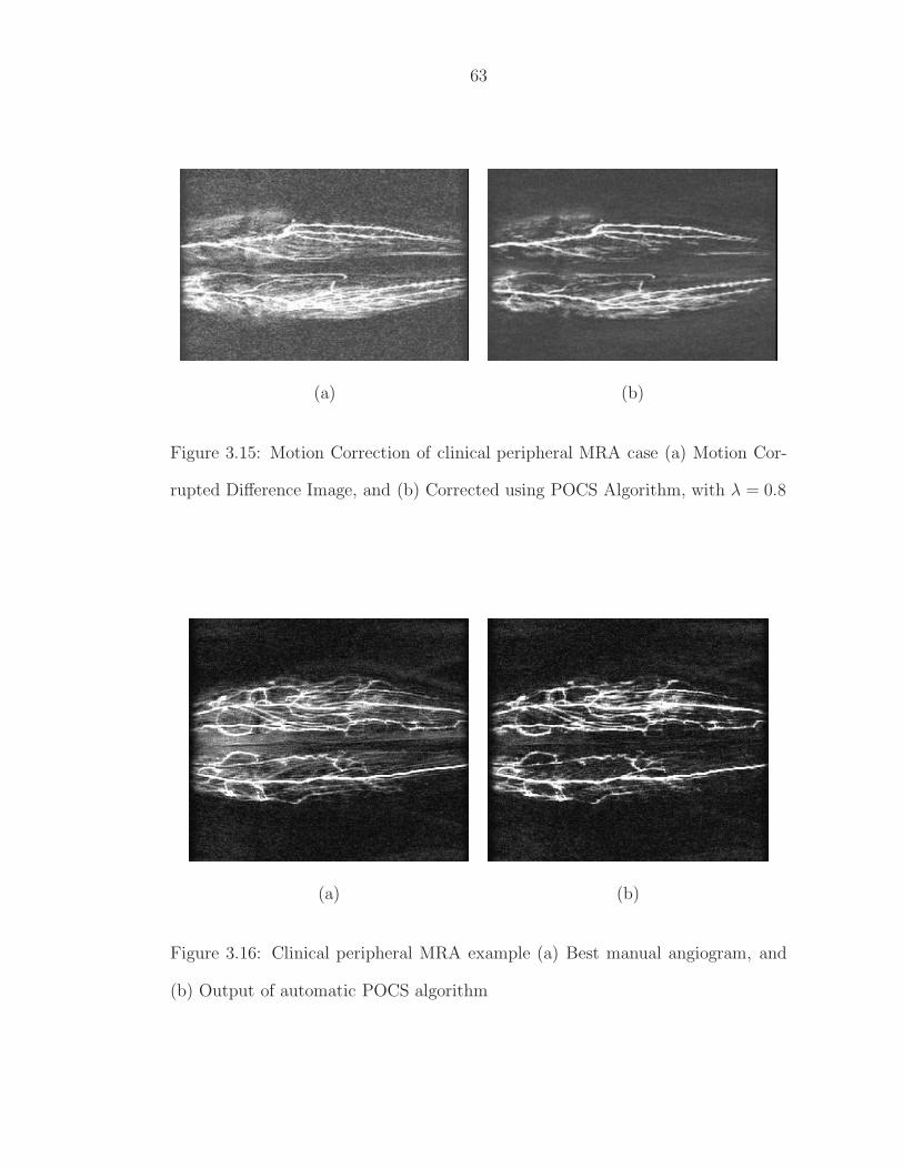
63

(a) (b)

Figure 3.15: Motion Correction of clinical peripheral MRA case (a) Motion Cor-

rupted Difference Image, and (b) Corrected using POCS Algorithm, with λ = 0.8

(a) (b)

Figure 3.16: Clinical peripheral MRA example (a) Best manual angiogram, and

(b) Output of automatic POCS algorithm

64

(a) (b)

Figure 3.17: Another example: (a) Best manual angiogram, and (b) Output of

automatic POCS algorithm

The example in figure 3.17, shown at a different contrast and saturation level,

shows up some limitations of the POCS algorithm. While there is significant

clutter reduction, there seems to be some loss of extremely fine or faint arterial

features. This example illustrates the need to strike a good balance between motion

suppression and loss of some fine features. On the other hand, the definition and

contrast of major arteries is enhanced by our method.

These examples suggest that motion correction inevitably involves some loss

of fine details despite careful design of the algorithm to prevent it. As such,

the method should only be used in cases where significant motion has occurred.

Also, since the best angiogram is obtained by averaging operations on the data

set, the removal of artifacts from individual frames may not necessarily lead to

commensurate improvement in the final angiogram.

In addition to visual evidence, an extensive double-blind comparative study

was conducted to validate the technique. A set of randomized image pairs was

presented to an experienced radiologist, one obtained manually by a specialist, and

65

the other obtained automatically by our technique as described above. A total of 47

cases were studied. The results are shown in Table 3.1. The mean score was 2.74,

on a scale from 1 to 5, with 1 denoting cases where the automatic POCS algorithm

performs much better than manual, and 5 denoting manual performing much better

than POCS. It is noteworthy that the number of cases where our result was deemed

better than the manually obtained result (25) exceeds the number of cases where

manual result outperformed our result (16). The last number mainly corresponds

to those cases which did not have motion artifacts to begin with, and whose fine

features got slightly degraded by the POCS algorithm which was attempting to

remove motion that was not there. Yet overall, the automatic method still does

significantly better than manual method. A two-tailed two-sample (paired) t-test

was conducted on the scores in the table. At 5% level of significance, the quality

score of POCS-corrected angiograms was found to be significantly better than

manually obtained angiograms (t(92) = −2.45, p = 0.0162). Clearly, such a small

p-value indicates significant improvement for real clinical cases. This presents a

strong justification for using the un-supervised method presented here in clinical

MRA exams, perhaps with some operator intervention to identify corrupted cases.

While our results do not indicate improvement over manual methods in all cases,

it may be pointed out that instances in the literature of completely automatic

algorithms even partially outperforming data obtained by an experienced medical

practitioner are relatively rare.

3.5.4 Limitations and further improvements

While there is strong visual and statistical evidence of the success of our method,

we also encountered several problems during the experimental evaluation. The

66

Table 3.1: Results of a Double Blind Comparison of Manual versus Automatic

POCS Angiograms

POCS >> man POCS > man same POCS < man POCS << man

3 22 6 16 0

main problem with the POCS algorithm remains the fact that in order to remove

artifacts resulting from motion, especially arbitrary 3D motion, it is frequently nec-

essary to constrain the time evolution of certain features in the complex frames.

We have provided theoretical and empirical evidence that the POCS algorithm usu-

ally leads to only small amounts of degradation of vascular enhancement. However,

the fact remains that the two goals of preserving useful data and removing arti-

facts are in a way mutually contradictory — there is always some, albeit small,

loss of vascular definition during the process. This problem manifests itself most

often when excessive amounts of artifacts bury small, fine vascular features. In

such cases one may have to settle at a conservative correction if one is interested

in these fine features. In other words, one must decide on the trade-off between

background motion clutter and resolution of fine features on a case-by-case basis.

This suggests the need for some operator involvement in selecting this trade-off

point. The automatic technique presented here relies on the accuracy of the mask

and arterial phase selection algorithm, called MR-DSA [KPZ+02]. Work currently

underway by several workers in this and other labs will likely result in dramatic

improvement in the MR-DSA classification algorithm, which will produce a cor-

responding improvement in the performance of the proposed automatic motion

correction method. In the meantime, our correction method can be applied in the

non-automatic mode, where an operator selects arterial and mask phases and iden-

67

tifies frames corrupted by motion. Further improvements may result from a hybrid

of the proposed method with other motion correction schemes like navigators or

parameter tracking methods. Work is continuing in this direction.

3.6 Conclusion

We have described a convex projection-based algorithm that corrects a motion cor-

rupted frame by iteratively making it more similar to a non-corrupted one. The

algorithm is able to identify and partially correct corrupted features of k-space and

thereby remove artifacts due to complex non-global or non-rigid motion. Radiolog-

ically important temporal events are not degraded by the successive projections.

The technique has the potential to retrieve corrupted angiography data that would

otherwise be unusable due to motion artifacts. Simulated and clinical examples

present visual evidence of the efficacy of our method. The POCS algorithm, af-

ter being incorporated into a completely automatic program, was found to yield

automatic angiogram results that were judged to show significant improvement

over manually obtained angiogram during a double-blind comparative study. The

method can be extended to 3D data, and is able to incorporate additional motion

correction innovations within the general POCS framework.

Chapter 4

Total Least Sense: A Maximum -

Likelihood Approach to Parallel MR

Imaging with Sensitivity Noise

Parallel imaging is a powerful technique to speed up Magnetic Resonance (MR)

image acquisition via multiple coils. Each coil subsamples in k-space at the cost

of introducing aliasing. The output of the coils, plus the sensitivity maps that

describe the different responses of each coil, can then be combined to produce a

non-aliased image. Widely used parallel imaging methods such as SENSE and

its variants assume that the coil outputs contain noise, but that the sensitivity

maps are noiseless. In practice, however sensitivity maps are subject to a wide

variety of errors. At first glance, sensitivity noise appears to result in an errors-

in-variables problem of the kind that is typically solved using Total Least Squares

(TLS). However, existing TLS algorithms are inappropriate for the specific type of

block structure that arises in parallel imaging. Here we take a maximum likelihood

approach to the problem of parallel imaging in the presence of independent Gaus-

sian sensitivity noise. This results in a quasi-quadratic objective function, which

can be efficiently minimized. Experiments demonstrate that our method produces

substantial SNR gains over current methods.

68

69

4.1 Parallel Imaging and Sensitivity Noise

Magnetic resonance imaging involves a fundamental trade-off between image qual-

ity and scan time [WBP04]. As described in chapter 2, parallel imaging techniques

like SENSE [PWSB01], SMASH [MOY+01] and GRAPPA [WND+03] use multiple

coils to reduce scan time. Our work concentrates on the SENSE technique since it

is widely recognized as the most general and powerful one. The sensitivity maps of

receiver coils are used to encode the imaging volume. These sensitivity maps are

typically obtained by scanning with a phantom. The outputs of each coil can be

combined with the sensitivity maps to reconstruct a full, unaliased image. Recall

that the reconstruction algorithm used by SENSE assumes that the output of the

receiver coils has been corrupted by noise, and can be modeled as

y = Ex + n, (4.1)

where n is Gaussian noise, assumed to be independent and identically distributed

(i.i.d.). This noise may arise, for example, from instrumentation error. The SENSE

method takes a least squares approach, which is natural under these assumptions.

Note that the least squares solution is well-known to be the maximum likelihood

estimate [PTVF92, Ch. 15], again assuming this noise model.

In this chapter we address a major shortcoming with SENSE, which is the

assumption that the sensitivity maps are noiseless. The sensitivity maps, however,

are computed from an MR scan, typically of a phantom. As a result, they are

subject to almost the same noise processes that affect the coil outputs during the

scans of the patients. This is not just a theoretical argument; we will demonstrate

in section 4.4 that our reconstruction method, which handles sensitivity noise,

gives significantly better experimental results.

70

As mentioned in chapter 1, we model the imaging process as

y = (E + ∆E)x + n, (4.2)

where ∆E is the noise in the system matrix that results from errors in the sensi-

tivity maps (i.e., sensitivity noise). At first glance, this appears to be an errors-in-

variables problem of the kind commonly addressed with Total Least Squares (TLS)

[HL02]. Indeed, several authors, such as [LBJ+02], have suggested taking a TLS

approach to sensitivity error. However, TLS algorithms assume that ∆E consists

of independent elements. The discussion of noise model in section 2.2 demonstrates

that this assumption is invalid, due to the block structure of the system matrix E

in parallel imaging.

We propose a maximum likelihood approach to solving equation (4.2). Maxi-

mum likelihood can be viewed as a generalization of both least squares [PTVF92]

and total least squares [HL02]. We use the natural model for sensitivity errors,

where each pixel in the sensitivity map is corrupted by i.i.d. noise. The resulting

algorithm, which we call TL-SENSE, gives strong results, even in cases where our

assumed noise model is incorrect. We show a couple of examples later where the

sensitivity errors do not follow the assumed model, but are still mitigated by our

method. A reasonable explanation for this phenomenon is that while out i.i.d.

noise assumption may be inaccurate for these cases, it is still much better than

the conventional assumption of zero sensitivity errors. This is by no means a novel

observation - for many years workers in signal processing, radar systems and mo-

bile communications, to give a few examples, have used i.i.d. Gaussian models to

great effect, even in cases where they are demonstrably inaccurate.

The rest of this chapter is organized as follows. We present our system model

(from §2.2) and our model for sensitivity noise. In §4.2 we discuss related work, and

71

show that sensitivity noise cannot be handled by standard methods such as TLS or

its variants. Section 4.3 derives our new TL-SENSE algorithm from a maximum

likelihood formulation. We also demonstrate that with Cartesian sampling the

general solution can be considerably simplified, and results in a quasi-quadratic

minimization problem directly in image space. We give experimental results on

both simulated and clinical data in section 4.4.

Recall from §2.2 that he output of the l-th coil is

yl = Elx = DHN×M ↓R DN×MSl · X = DH

N×M ↓R DN×Mdiag(sl)x. (4.3)

Also recall that the entire multi-coil output can be written as

y = [yT1 , . . . , yT

L]T ,

E = [ET1 , . . . , ET

L ]T

Similarly, the k-space version becomes

y = [yT1 , . . . , yT

L]T ,

E = [ET1 , . . . , ET

L ]T

4.1.1 System matrix structure under Cartesian sampling

The vast majority of MR scans are done with regular Cartesian sampling in k-space,

which considerably simplifies the problem and produces a specific matrix structure.

The 2-D DFT operator then reduces to two 1-D DFT’s acting separately on rows

and columns. The general-purpose k-space sampling operator ↓R in equation (4.3)

is now redefined as a sub-sampling operator, equivalent to removing rows of k-space.

Writing DN×M = DrowM Dcol

N as the explicit row and column 1-D DFT operations,

since ↓R only acts on columns, we have ↓R DN×M = DrowM ↓R Dcol

N . The output

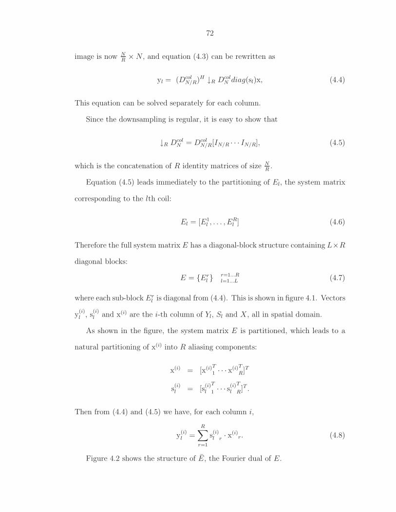
72

image is now NR× N , and equation (4.3) can be rewritten as

yl = (DcolN/R)H ↓R Dcol

N diag(sl)x, (4.4)

This equation can be solved separately for each column.

Since the downsampling is regular, it is easy to show that

↓R DcolN = Dcol

N/R[IN/R · · · IN/R], (4.5)

which is the concatenation of R identity matrices of size NR

.

Equation (4.5) leads immediately to the partitioning of El, the system matrix

corresponding to the lth coil:

El = [E1l , . . . , E

Rl ] (4.6)

Therefore the full system matrix E has a diagonal-block structure containing L×R

diagonal blocks:

E = Erl r=1...R

l=1...L (4.7)

where each sub-block Erl is diagonal from (4.4). This is shown in figure 4.1. Vectors

y(i)l , s

(i)l and x(i) are the i-th column of Yl, Sl and X, all in spatial domain.

As shown in the figure, the system matrix E is partitioned, which leads to a

natural partitioning of x(i) into R aliasing components:

x(i) = [x(i)T

1 · · · x(i)T

R]T

s(i)l = [s

(i)l

T

1 · · · s(i)l

T

R]T .

Then from (4.4) and (4.5) we have, for each column i,

y(i)l =

R∑r=1

s(i)l r · x(i)

r. (4.8)

Figure 4.2 shows the structure of E, the Fourier dual of E.

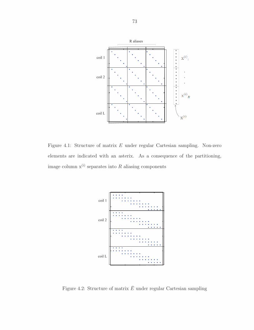
73

coil 1

coil 2

coil L

R aliases

*

*

*

*

*

**

*

*

*

*

**

*

*

*

*

*

.

.

.

Figure 4.1: Structure of matrix E under regular Cartesian sampling. Non-zero

elements are indicated with an asterix. As a consequence of the partitioning,

image column x(i) separates into R aliasing components

coil 1

coil 2

coil L

Figure 4.2: Structure of matrix E under regular Cartesian sampling

74

To maintain readability, we will henceforth drop the superscript (i) denoting

the ith column. We will use the same symbols E, x and y etc. both for arbitrary

and Cartesian sampling, with their meaning being indicated from the context.

4.1.2 System matrix structure under arbitrary sampling

The system matrices E, E have important special forms. The individual blocks

E1, . . . , EL have a Toeplitz structure as shown in figure 4.2, but they have been

decimated by the sampling. (Recall that a Toeplitz matrix is a matrix T = Tij

such that Tij = tj−i for a given row vector t.) If the sampling were not present,

the matrix E would have Toeplitz block structure.

The Toeplitz-type structure of each block results from the convolution operation

in k-space. The decimation of rows results from the subsampling of data points

in k-space. The structure of the corresponding image-space matrix E can be

determined from (4.3) for arbitrary k-space sampling. Unlike the simple closed-

form diagonal-block structure that arises in Cartesian sampling, this structure can

be quite complicated as it depends on the sampling trajectories used.

4.1.3 Our noise model

We use the obvious noise model of i.i.d. Gaussian noise both for sensitivity and

instrumentation noise. We note that the Gaussian assumption is only valid for

complex data; once an actual image is obtained by discarding phase information,

the noise process accociated with such images is well-known to be Rician rather

than Gaussian [GBD04]. Here the quentities involved are complex, hence the

Gaussian assumption is valid. For l ∈ 1, . . . , L, the noise model for the lth coil

75

sensitivity and output, respectively, is given by

Snoisyl = Sl + N s

l (4.9)

Y noisyl = Yl + Nl (4.10)

where the output noise terms Nl are i.i.d. Gaussian with standard deviation σn,

and sensitivity noise terms N sl are i.i.d. Gaussian with standard deviation σns . Let

nl and nsl be their vectorized representations.

Clearly, the structure of E must mimic that of E shown in figure 4.1:

E = Erl r=1...R

l=1...L , (4.11)

and the same holds for the k-space versions E and E. Again, each sub-block Erl

is diagonal, with entries given by the sensitivity map noise terms N sl . Similarly, in

k-space the error matrix E mimics the structure of E as shown in figure 4.2.

The assumption of Gaussian noise in spatial sensitivity measurement is actu-

ally quite a natural one, since sensitivity maps are usually obtained through an

initial scan with a uniform phantom. As a result, the effects of measurement noise

clearly carry over into sensitivity maps. The effect of this noise can frequently

be exacerbated by further processing, like the common practice of dividing by the

body coil output, or the sum-of-squares from all coils [PWBB01]. In addition,

by using two separate scans for sensitivity and data, certain other small errors or

discrepancies can creep in the actual sensitivity map as compared to the measured

sensitivity maps.1 In practical experiments involving phased array coils such dis-

crepancies result from small changes in orientation and positioning of coils, coil

loading effects, non-systematic coil and instrumentation errors, as well as a host

1This is why we explicitly allow for the noise variance of coil output and coilsensitivity to be different.

76

of other errors resulting from random noise. In the absence of a detailed and ex-

haustive error model for parallel imaging, the noise resulting from all these effects

may reasonably be assumed to be i.i.d. Gaussian.

If the noise cannot be modelled accurately as i.i.d. white noise, or if the

noise variance of the coils are different, it is easy to incorporate a more general

non-identically distributed non-white noise model, by pre-multiplying E with a

“whitening” matrix, as described above for coil output data. All correlation be-

tween different coils and sensitivity noise from the same coil can thus be removed,

and we may continue using the i.i.d. Gaussian model.

4.2 Related Work

Equation (4.2) appears to be an errors-in-variables problem of the kind tradition-

ally solved with TLS. Such methods appear not to have been applied to parallel

imaging. This may result from the fact that TLS makes extremely unrealistic as-

sumptions about the structure of the sensitivity noise. There are variants of TLS,

such as Constrained Total Least Squares, that can handle a broad class of matrix

structure, including the structures that arise in parallel imaging. However, these

approaches require the use of very general minimization techniques, which are very

inefficient.

4.2.1 Total Least Squares

The classical TLS theory [GL96] applied on (4.2) attempts to find a solution that

minimizes both the additive noise n as well as the error-in-variables E, as follows:

xTLS = arg minx

|| [E | n] ||F , subject to n + Ex = y − Ex (4.12)

77

where the indicated norm is the Frobenius norm over a matrix obtained by concate-

nating E and n. Note that this problem formulation assumes that the elements

of E are independent (i.e., that E has no structure).

Unfortunately, TLS is ill-equipped to handle the specific system model de-

scribed in §4.1.3. This is because E has a diagonal block structure as shown in

figure 4.1, with off-diagonal elements in the constituent blocks being zero. The

corresponding elements of E will therefore also be zero. As a consequence, the

independence assumption of TLS is always violated, even when the underlying

sensitivity noise process is independent.

A similar situation results if one tries to perform classical TLS on the k-space

imaging model (2.1). The system matrix E derives from the convolution operator,

leading to a Toeplitz-type structure as shown in figure 4.2. This results in the

elements of E, and consequently the elements of E, being algebraically related

to each other, rather than being independent variables.

4.2.2 Constrained Total Least Squares

Several generalizations of TLS have been proposed which handle matrix structure.

The best-known such technique is called Constrained TLS.2 The Constrained TLS

approach was proposed by [AMH91], whose work handles linearly structured matri-

ces — those matrices that can be obtained from a linear combinations of a smaller

perturbation vector.

For a linearly structured matrix E, the CTLS approach works as follows. Let

C = [E|y], and define a perturbation in C as C = [E|n]. CTLS consists of

2An earlier approach, called Structured TLS [MGK95], was shown to be equiv-alent to Constrained TLS in [LdMH96].

78

solving

minv,x

||v||, (4.13)

subject to

(C + C)

x

−1

= 0

and

C = [F1v|F2v| · · · |FN+1v],

where the Fi’s generate the elements of the linearly structured matrix ∆C . Note

that this problem is difficult to solve for an arbitrary linearly structured matrix E,

requiring the use of a general-purpose constrained minimization algorithm.

The system matrix that results from parallel MR (described in §2.2) turns out

to be linearly structured. However, by taking advantage of the particular structure

of the system matrix, we can use much more efficient special-purpose unconstrained

minimization methods.

4.3 The TL-SENSE Algorithm

We will derive a formula for (x), the likelihood of an image x, using the system

model and noise model of section 4.1.3. The TL-SENSE algorithm maximizes (x),

which involves minimizing a quasi-quadratic objective function. Under Cartesian

k-space sampling this objective function can be efficiently minimized using non-

linear least squares.

4.3.1 Deriving the likelihood function (x)

We now derive a formula for the likelihood (x) given the observed data y, which

is by definition Pr(y|x). Define the total noise by g(x) = y−Ex. Under the noise

79

model described in section 4.1.3, this is jointly Gaussian with zero mean. As a

result, and we can express the likelihood as

(x) ∝ exp(−1

2(y − Ex)HR−1

g|x(y − Ex)) (4.14)

where Rg|x = E((g(x))(g(x))H ) is the covariance matrix of the conditional noise

g(x)|x.

The maximum likelihood estimate, which we will denote x, minimizes− log (x),

and is given by

x = arg minx

(y − Ex)HR−1g|x(y − Ex). (4.15)

Under our noise model, Rg|x = E(nnH + (Ex)(Ex)H), and E(nnH ) = σ2nI .

Note that we have omitted the det(R−1g|x) term, for several reasons. This term re-

sults in an additional log term, making the overall cost function very expensive to

compute and analyse. However, the incremental benefit of including this term is

quite small since a log function does not increase as fast as the the rest of the cost

function, and can be safely neglected, especially when the initial “guess” of x is

sufficiently close to the correct estimate. Therefore equation (4.14) entails, strictly

speaking, an approximation of the Gaussian assumption. We point out that this

is a standard omission in many inversion problems. For example, in some image

restoration problems [MGK95], a careful experimentation with Toeplitz systems

exhibited little or no improvement in performance after the log term was included,

at substantial computational cost. Similar behaviour was observed during our ex-

perimentation. Consequently, we shall henceforth drop this term from discussion.

The data-dependent covariance E((Ex)(Ex)H) is an L × L block matrix[(Elx)(El′x)H

]l,l′∈1,...,L with the (l, l′)-th block (Elx)(El′x)H is given by

DHN/R×M ↓R DN×Mdiag(x)E(slsH

l′ )diag(x)DHN×M ↓H

R DN/R×M . This follows

from:

80

Elx = DHN/R×M ↓R DN×Mdiag(sl)x

= DHN/R×M ↓R DN×Mdiag(x)sl.

Due to our noise model, E(slsHl′ ) = σ2

nsδl,l′I . It follows therefore that

Rg|x = σ2n

I + β2

A(x)

. . .

A(x)

, (4.16)

where A(x) = DHN/R×M ↓R DN×Mdiag(|x|2)DH

N×M ↓HR DN/R×M , and β = σns/σn.

Finally, we have

R−1g|x =

1

σ2n

B(x)−1

. . .

B(x)−1

, (4.17)

where B(x) = I + β2DHN/R×M ↓R DN×Mdiag(|x|2)DH

N×M ↓HR DN/R×M . Due to the

block-diagonality, we can write the maximum likelihood estimate as

x = arg minx

∑l

(yl −Elx)HB(x)−1(yl − Elx). (4.18)

In summary, the TL-SENSE algorithm computes the maximum likelihood estimate

given by equation (4.18). Minimizing this expression is numerically expensive in

general. We discuss strategies for doing this in the next section, both for arbitrary

sampling as well as Cartesian sampling.

4.3.2 Minimization Algorithms

Solving equation (4.18) requires solving a non-quadratic minimization problem.

As a general rule, this would require a large number of cost function evaluations,

81

over a solution space of extremely large dimensionality. We now describe an effi-

cient strategy for the arbitrary sampling case. We will also show that in the case

of Cartesian sampled data, (4.18) can be reduced drastically in complexity, and

propose an efficient algorithm.

Each function evaluation of (4.18) for general, arbitrarily sampled data involves

the inversion of NM × NM matrices. Direct inversion is not a good option since

these matrices are unlikely to be sparse for arbitrary sampling schemes. However,

these inversions may be efficiently performed iteratively, since the products Bx and

BHx can be computed at O(NM log(N)) cost due to the presence of the Fourier

operator. Furthermore, B is obviously well-conditioned, which means that a fast

iterative algorithm like Preconditioned CG [GL96] can perform this inversion in

relatively few steps. Since the cost function may be expressed as a data-dependent

weighted least squares problem, powerful non-linear least squares algorithms may

be used to solve the problem efficiently (see [PTVF92, Ch. 10]). The TL-SENSE

solution (4.18) not only reduces drastically in complexity, but is only moderately

more expensive than the standard SENSE algorithm. We now turn to the special

but important case of Cartesian sampling, and obtain an efficent algorithm.

In order to minimize equation (4.18) under Cartesian sampling, we can apply

equation 4.8 with B(x(i)) = diag(1+β2∑R

r=1 |x(i)r |2). This being diagonal, the ML

problem reduces, like standard SENSE, to NM/R subproblems, each with only R

variables. In this section, we describe our non-linear least squares (NLLS) method

with Newton iterations.

From the above and the matrix structure of figure 4.1, the cost minimization

can be performed independently over aliasing elements in image space. Figure 4.3

shows the algorithm to minimize (4.8), one column at a time.

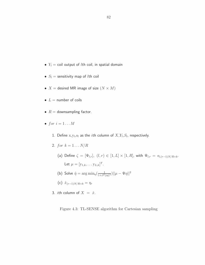
82

• Yl = coil output of lth coil, in spatial domain

• Sl = sensitivity map of lth coil

• X = desired MR image of size (N ×M)

• L = number of coils

• R = downsampling factor.

• for i = 1 . . . M

1. Define x,yl,sl as the ith column of X,Yl,Sl, respectively.

2. for k = 1 . . . N/R

(a) Define ζ = [Ψl,r], (l, r) ∈ [1, L] × [1, R], with Ψl,r = sl,(r−1)N/R+k.

Let µ = [y1,k, . . . yL,k]T .

(b) Solve η = arg minη(1

1+β2||η||2 )||µ − Ψη||2

(c) x(r−1)N/R+k = ηr

3. ith column of X = x.

Figure 4.3: TL-SENSE algorithm for Cartesian sampling

83

The minimization in figure 4.3 is challenging due to the presence of the non-

quadratic term. But the non-quadraticity enters the equation only via a well-

behaved, smooth, slowly-varying function of the norm ||η||2. Consequently, we can

perform the minimization using a non-linear least-squares method to solve

η = arg minη

||F (η)||2, F (η) = q(η)(µ − Ψη), q(η) = 1/√

1 + β2||η||2. (4.19)

This is similar to the standard least squares method for solving the pseudoin-

verse Ψ†. The only difference is that the Jacobian of F is not a constant matrix

any more. Fortunately, the Jacobian in this case is readily available and easily

computed. It is easily shown that

J(η) =∂F (η)

∂η= −q(η) · (Ψ + β2q2(η)(µ − Ψη)ηT ). (4.20)

The additional cost of non-quadratic minimization is not significantly higher than

the function evaluation used in standard pseudoinverse computed through conju-

gate gradients, due to the easy availability of the Jacobian and its cheap evaluation

from (4.20). The algorithm in figure 4.3 was implemented in MATLAB version

R13. Typical execution times for reconstructions of size 256 x 256 were between

three to four times the execution time in Matlab of standard SENSE.

4.4 Results

4.4.1 Simulation results

Cartesian TL-SENSE results were obtained from the following simulation: Sensi-

tivity maps of circular coils positioned uniformly around the FOV are computed

from the Biot-Savart Law. Coil output from each coil is computed by encoding a

Nyquist-sampled full MR image with the coil sensitivity map, followed by down

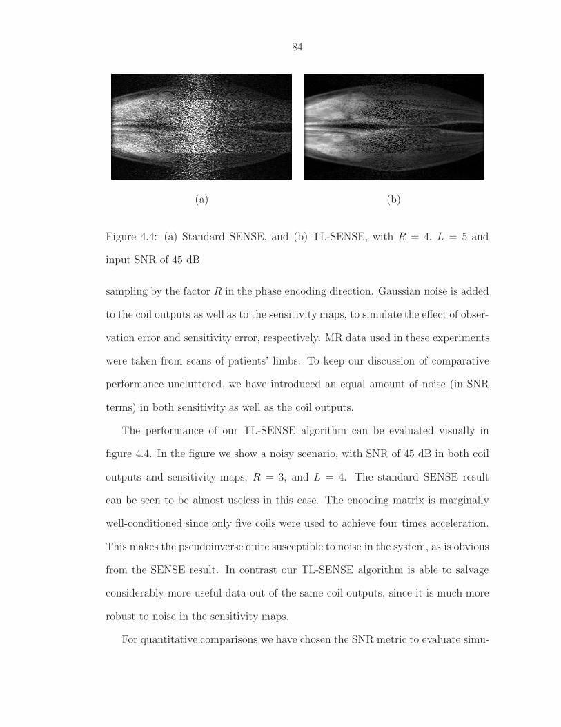
84

(a) (b)

Figure 4.4: (a) Standard SENSE, and (b) TL-SENSE, with R = 4, L = 5 and

input SNR of 45 dB

sampling by the factor R in the phase encoding direction. Gaussian noise is added

to the coil outputs as well as to the sensitivity maps, to simulate the effect of obser-

vation error and sensitivity error, respectively. MR data used in these experiments

were taken from scans of patients’ limbs. To keep our discussion of comparative

performance uncluttered, we have introduced an equal amount of noise (in SNR

terms) in both sensitivity as well as the coil outputs.

The performance of our TL-SENSE algorithm can be evaluated visually in

figure 4.4. In the figure we show a noisy scenario, with SNR of 45 dB in both coil

outputs and sensitivity maps, R = 3, and L = 4. The standard SENSE result

can be seen to be almost useless in this case. The encoding matrix is marginally

well-conditioned since only five coils were used to achieve four times acceleration.

This makes the pseudoinverse quite susceptible to noise in the system, as is obvious

from the SENSE result. In contrast our TL-SENSE algorithm is able to salvage

considerably more useful data out of the same coil outputs, since it is much more

robust to noise in the sensitivity maps.

For quantitative comparisons we have chosen the SNR metric to evaluate simu-

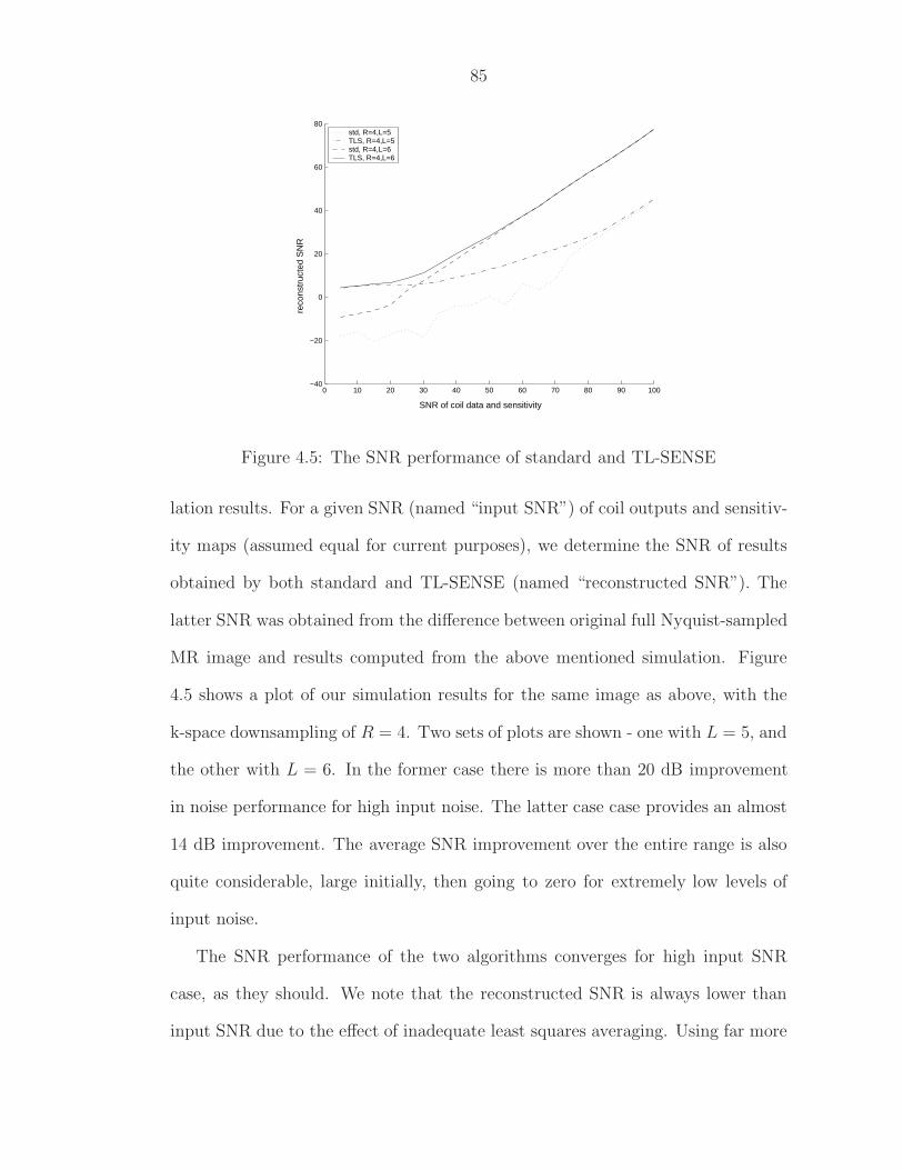
85

0 10 20 30 40 50 60 70 80 90 100−40

−20

0

20

40

60

80

SNR of coil data and sensitivity

reco

nstr

ucte

d S

NR

std, R=4,L=5TLS, R=4,L=5std, R=4,L=6TLS, R=4,L=6

Figure 4.5: The SNR performance of standard and TL-SENSE

lation results. For a given SNR (named “input SNR”) of coil outputs and sensitiv-

ity maps (assumed equal for current purposes), we determine the SNR of results

obtained by both standard and TL-SENSE (named “reconstructed SNR”). The

latter SNR was obtained from the difference between original full Nyquist-sampled

MR image and results computed from the above mentioned simulation. Figure

4.5 shows a plot of our simulation results for the same image as above, with the

k-space downsampling of R = 4. Two sets of plots are shown - one with L = 5, and

the other with L = 6. In the former case there is more than 20 dB improvement

in noise performance for high input noise. The latter case case provides an almost

14 dB improvement. The average SNR improvement over the entire range is also

quite considerable, large initially, then going to zero for extremely low levels of

input noise.

The SNR performance of the two algorithms converges for high input SNR

case, as they should. We note that the reconstructed SNR is always lower than

input SNR due to the effect of inadequate least squares averaging. Using far more

86

coils than strictly required for acceleration will lead to improved SNR performance

overall. Already, going from L = 5 to L = 6 results in significant SNR gain.

The figure also shown an interesting but expected trend - the SNR gain due to

TL-SENSE becomes smaller for better conditioned, more over-determined systems.

This is expected because a highly over-determined, well-conditioned system should

be able to overcome the effect of noise in the system model more effectively than

marginally conditioned ones. The SNR improvement shown in the figure for noisy

cases is quite significant, amounting to almost a hundred times reduction of the

noise energy! This improvement was achieved from the same data set and for

modest additional computation time (of the order of a few minutes, in MATLAB

R13) as compared to standard SENSE.

4.4.2 Experiments with Sensitivity mismatch on phantom

data

Phased array experiments were performed with a high-resolution (HiRes) phantom

as the target, and a uniform spherical phantom to generate sensitivity maps. These

experiments were mainly performed to demonstrate the use of our technique even

for cases where sensitivity noise is not dominated by i.i.d. Gaussian noise, but

other sources of errors like sensitivity mismatch and insufficient FOV. The HiRes

phantom was placed within a plastic tube filled with doped water, and torso coil

pads were wrapped around the tube. In order to acheive sufficient resolution of

the target, the FOV was chosen to be smaller than the diameter of the plastic

tube. This results in controlled aliasing in the reconstructed coil data. Sensitivity

maps were obtained under the same conditions with the uniform phantom, but

now in addition to the uniform phantom signals, we also have contributions from

87

the tube, which also has a uniform response. Un-aliased data received by one coil

within the 4-coil configuration is shown in figure 4.6. Notice that sensitivity re-

sponse has some contributions from the tube, of unequal intensity to the uniform

phantom inside it. This state of affairs is usually quite disastrous for conventional

parallel imaging. In addition, a small mis-alignment of the image was also ob-

served between the sensitivity data and the HiRes data. While this experiment

does not follow the standard parallel imaging set up, it mimics in many ways the

kinds of errors one can expect if sensitivity maps are mis-aligned, incorrect, or

obtained by improper division with a body coil image. The purpose of the exper-

iment was to determine the extent to which such a complicated data set can be

reconstructed under gross inaccuracies in sensitivity data. These errors are quite

unlike the noise model we assumed in this work, and we would like to see if the

technique is still effective. The reconstruction results are shown in figure 4.7. In

addition to standard SENSE, we also show for comparison a Tikhonov-regularized

version of SENSE. This should address the question of whether these errors can

be mitigated simply by regularizing the SENSE reconstruction. It is obvious that

while the standard SENSE method results in considerable errors due to mismatch

and aliasing in the original data, this error can not be easily removed even by

regularizing. The noise levels go down with higher regularization factors, but at

the cost of degraded unfolding performance. This is an expected result - in the

limit when regularization parameter is very large, the matrix inverse corresponds

to a copy of the observation, i.e. no unfolding. The TL-SENSE result on the

other hand is quite a lot more effective at both noise reduction as well as image

unfolding. The effect of sensitivity mismatch and aliasing problems is visible, but

considerably muted compared to SENSE results. The result seems to suggest that

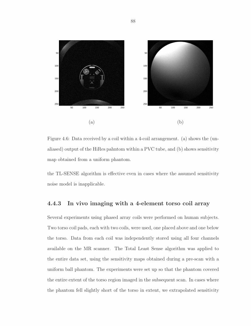
88

50 100 150 200 250

50

100

150

200

250

50 100 150 200 250

50

100

150

200

250

(a) (b)

Figure 4.6: Data received by a coil within a 4-coil arrangement. (a) shows the (un-

aliased) output of the HiRes pahntom within a PVC tube, and (b) shows sensitivity

map obtained from a uniform phantom.

the TL-SENSE algorithm is effective even in cases where the assumed sensitivity

noise model is inapplicable.

4.4.3 In vivo imaging with a 4-element torso coil array

Several experiments using phased array coils were performed on human subjects.

Two torso coil pads, each with two coils, were used, one placed above and one below

the torso. Data from each coil was independently stored using all four channels

available on the MR scanner. The Total Least Sense algorithm was applied to

the entire data set, using the sensitivity maps obtained during a pre-scan with a

uniform ball phantom. The experiments were set up so that the phantom covered

the entire extent of the torso region imaged in the subsequent scan. In cases where

the phantom fell slightly short of the torso in extent, we extrapolated sensitivity

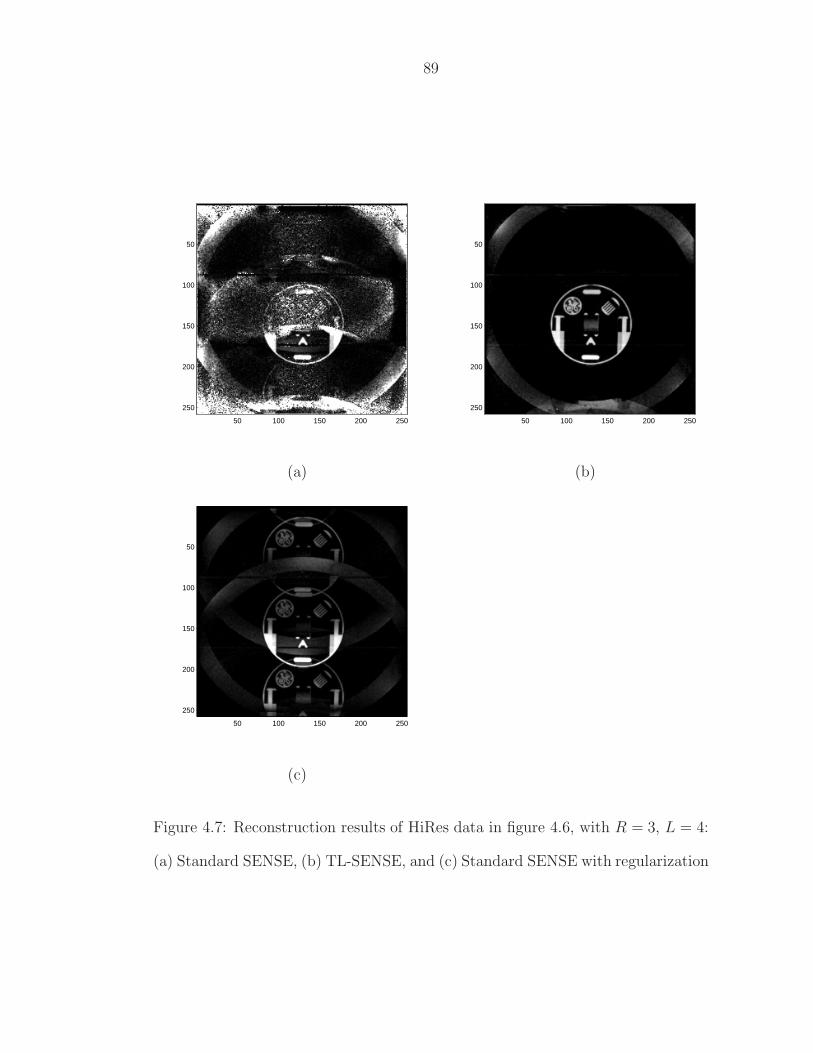
89

50 100 150 200 250

50

100

150

200

250

50 100 150 200 250

50

100

150

200

250

(a) (b)

50 100 150 200 250

50

100

150

200

250

(c)

Figure 4.7: Reconstruction results of HiRes data in figure 4.6, with R = 3, L = 4:

(a) Standard SENSE, (b) TL-SENSE, and (c) Standard SENSE with regularization

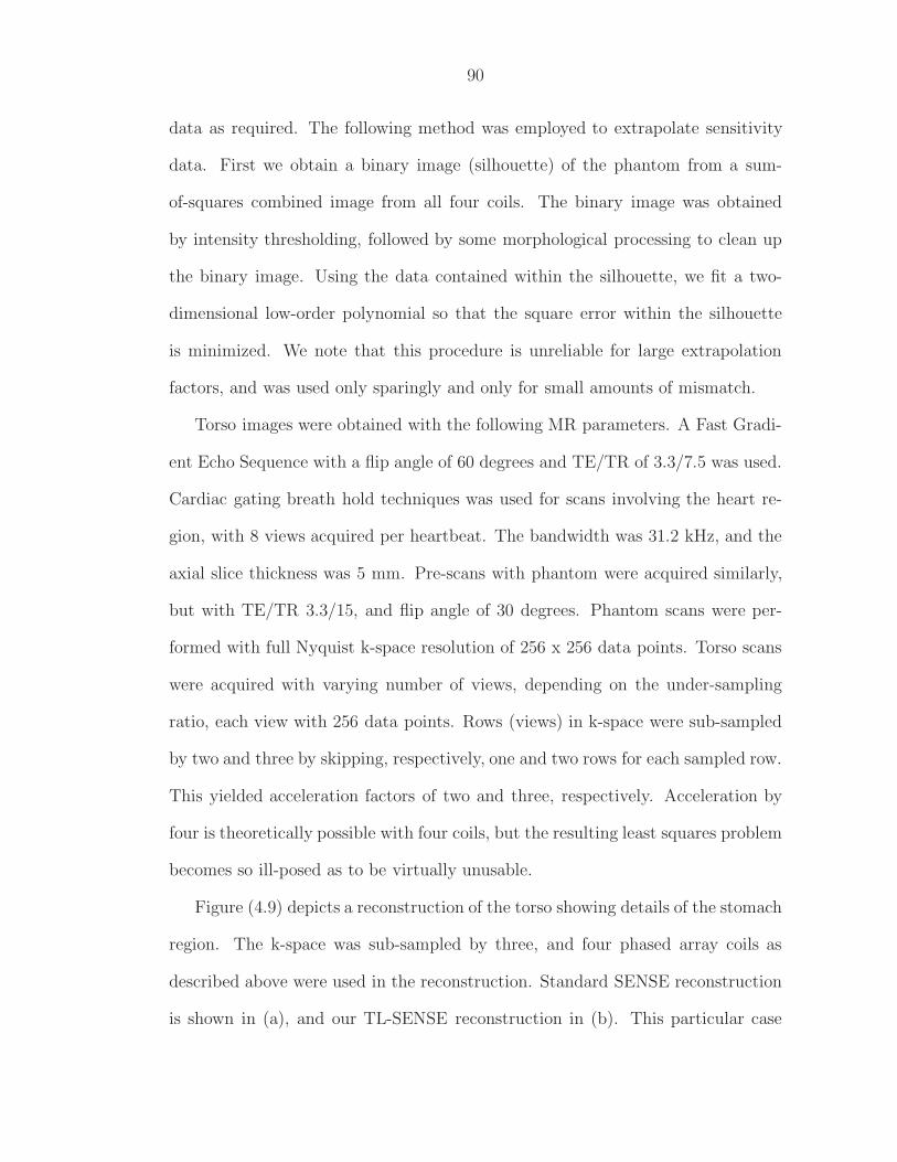
90

data as required. The following method was employed to extrapolate sensitivity

data. First we obtain a binary image (silhouette) of the phantom from a sum-

of-squares combined image from all four coils. The binary image was obtained

by intensity thresholding, followed by some morphological processing to clean up

the binary image. Using the data contained within the silhouette, we fit a two-

dimensional low-order polynomial so that the square error within the silhouette

is minimized. We note that this procedure is unreliable for large extrapolation

factors, and was used only sparingly and only for small amounts of mismatch.

Torso images were obtained with the following MR parameters. A Fast Gradi-

ent Echo Sequence with a flip angle of 60 degrees and TE/TR of 3.3/7.5 was used.

Cardiac gating breath hold techniques was used for scans involving the heart re-

gion, with 8 views acquired per heartbeat. The bandwidth was 31.2 kHz, and the

axial slice thickness was 5 mm. Pre-scans with phantom were acquired similarly,

but with TE/TR 3.3/15, and flip angle of 30 degrees. Phantom scans were per-

formed with full Nyquist k-space resolution of 256 x 256 data points. Torso scans

were acquired with varying number of views, depending on the under-sampling

ratio, each view with 256 data points. Rows (views) in k-space were sub-sampled

by two and three by skipping, respectively, one and two rows for each sampled row.

This yielded acceleration factors of two and three, respectively. Acceleration by

four is theoretically possible with four coils, but the resulting least squares problem

becomes so ill-posed as to be virtually unusable.

Figure (4.9) depicts a reconstruction of the torso showing details of the stomach

region. The k-space was sub-sampled by three, and four phased array coils as

described above were used in the reconstruction. Standard SENSE reconstruction

is shown in (a), and our TL-SENSE reconstruction in (b). This particular case

91

Figure 4.8: Aliased coil data from a torso scan with R = 3, L = 4

possessed reasonably good conditioning properties, and the reconstruction was

well-posed for both standard and TL-SENSE solutions. The data suffered from

random instrumentation noise as well as some amounts of i.i.d. sensitivity noise,

resulting in unwanted noise amplification during standard reconstruction. The

TL-SENSE reconstruction in contrast does not exhibit this noise amplification to

any significant extent.

Figure (4.10) depicts the same torso slice as above, but this time with some

mismatch in measured and actual sensitivity maps. The mismatch was a result

of using flexible torso pads without rigid fastenings - a common issue with torso

coils. The k-space was sub-sampled by three, and four phased-array coils as de-

scribed above were used in the reconstruction. Conditioning of the encoding matrix

was again reasonably good, and the reconstruction was well-posed. However, the

data suffered from some instrumentation noise apart from sensitivity mismatch,

resulting in unwanted noise amplification artifacts during standard reconstruction.

92

(a) (b)

Figure 4.9: Reconstruction results of torso data from figure 4.8: (a) Standard

SENSE, and (b) TL-SENSE, with R = 3, L = 4

The TL-SENSE reconstruction however does not suffer from these reconstruction

artifacts.

4.4.4 Parallel Brain Imaging With An 8-Element Head

Coil

For our next experiment, we scanned some brain data using an eight-element head

coil, one channel per element. The acceleration factor was R = 4. Figure 4.12

shows the results. The standard SENSE reconstruction, shown in (a), leads to

too much noise amplification. In order to demonstrate that this problem cannot

really be addressed by simply performing regularization on the SENSE method,

we show in (b) the output of a Tikhonov-regularized SENSE algorithm, with the

regularization factor set at 0.1, chosen after several trials with other values. While

this procedure is considerably less noise-prone, it has in fact failed to resolve the

aliasing components properly. A smaller value of regularization, say 0.05, would

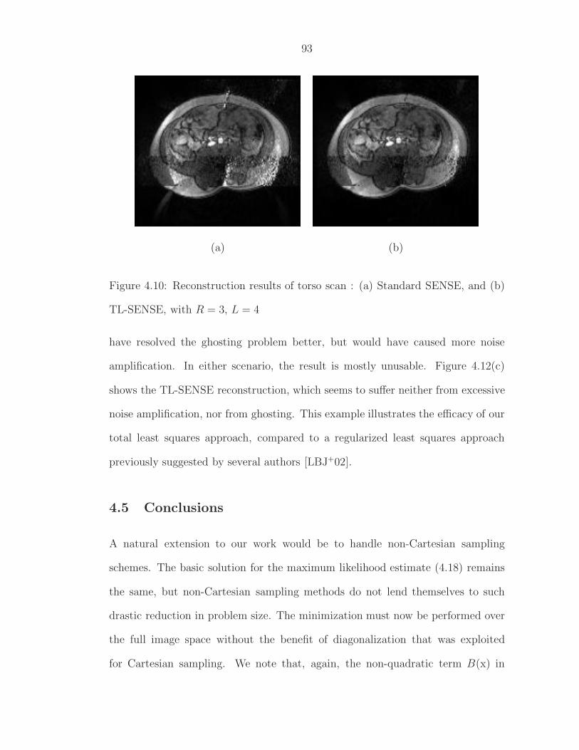
93

(a) (b)

Figure 4.10: Reconstruction results of torso scan : (a) Standard SENSE, and (b)

TL-SENSE, with R = 3, L = 4

have resolved the ghosting problem better, but would have caused more noise

amplification. In either scenario, the result is mostly unusable. Figure 4.12(c)

shows the TL-SENSE reconstruction, which seems to suffer neither from excessive

noise amplification, nor from ghosting. This example illustrates the efficacy of our

total least squares approach, compared to a regularized least squares approach

previously suggested by several authors [LBJ+02].

4.5 Conclusions

A natural extension to our work would be to handle non-Cartesian sampling

schemes. The basic solution for the maximum likelihood estimate (4.18) remains

the same, but non-Cartesian sampling methods do not lend themselves to such

drastic reduction in problem size. The minimization must now be performed over

the full image space without the benefit of diagonalization that was exploited

for Cartesian sampling. We note that, again, the non-quadratic term B(x) in

94

Figure 4.11: Aliased coil data from a head scan with R = 4, L = 8

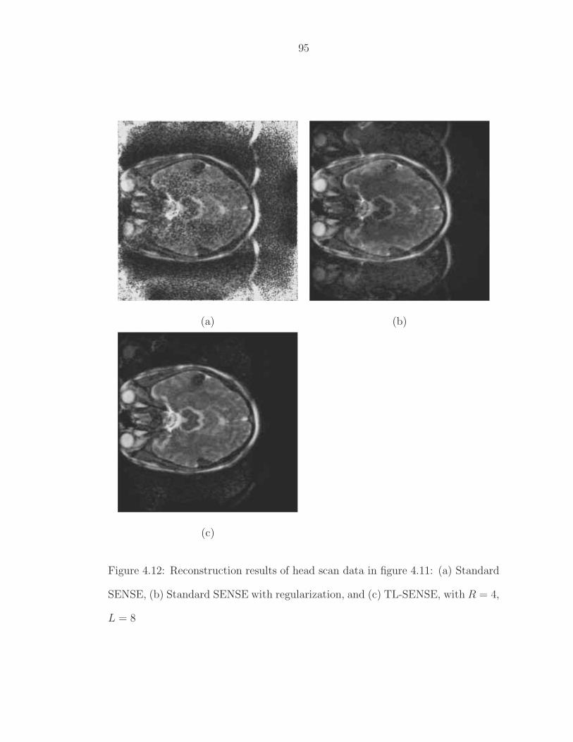
95

(a) (b)

(c)

Figure 4.12: Reconstruction results of head scan data in figure 4.11: (a) Standard

SENSE, (b) Standard SENSE with regularization, and (c) TL-SENSE, with R = 4,

L = 8

96

(4.18) is rather well-behaved compared to the quadratic cost term. Hence, we may

again utilize non-linear least squares techniques using Newton-type direction search

to compute the minimum. The evaluation of the Jacobian and Hessian is again

expected to be cheap due to its block-diagonal nature. For arbitrary sampling

schemes therefore we expect our algorithm to be of the same order of complexity

as standard SENSE algorithms.

We have addressed the problem of obtaining an optimal solution to the parallel

imaging reconstruction problem in the presence of both measurement and sensi-

tivity noise. We have shown that for i.i.d. Gaussian noise the optimal solution is

the minimizer of a weakly non-quadratic objective function which may be solved

efficiently via a non-linear least squares iterative technique with modest additional

complexity compared to standard SENSE algorithms. We have also derived sim-

plified expressions for the cost function as well as the Jacobian of the associated

least squares problem in the case of Cartesian k-space sampling. A fast Newton

algorithm with explicit Jacobian information was developed to solve the problem.

Results for Cartesian k-space sampling indicate impressive improvement in per-

formance compared to standard SENSE, amounting to almost 20 dB SNR gain

in several high-noise cases. The algorithm yields substantial improvement even in

cases where the i.i.d. Gaussian sensitivity noise model implicit in the method is

not accurate.

Chapter 5

A Graph Cut Energy Minimization

Algorithm for a New Class of Pixel

Labeling Problems

5.1 Introduction

A large number of Bayesian estimation problems that arise in medical imaging,

signal and image processing and machine vision can benefit immensely from a

Markov Random Field (MRF) based formulation of a priori information. It is well-

known that the MRF approach is a powerful and natural way to exploit spatial

redundancy present in multi-dimensional data. These problems typically require

inverting a linear system. The MRF approach has found favour in some recent

work in image restoration as well as vision problems like stereo. In this chapter

we propose the use of this approach for enhanced MR reconstruction from parallel

data - in other words exploit both receiver redundancy from multiple coils as

well as spatial redundancy in the form of a spatial prior. It turns out that the

same class of techniques can perform Bayesian estimation in a large number of

linear systems, essentially any problem which involves the estimation of multi-

dimensional spatially correlated signals. Hence we will formulate the problem in

terms of general linear systems, develop our technique in general terms, and then

97

98

specialize to particular applications. The main restriction of our technique is that

it works only on linear systems with non-negative matrix elements. We will show

that Cartesian parallel MR reconstruction problems fall under this category, as

do many other problems in vision and image processing. We will motivate our

approach by discussing linear systems arising in Vision; then we will extend the

discussion to MR reconstruction.

All these linear problems can be made well-posed by adding a regularization

term; this term imposes spatial smoothness, and should preserve discontinuities.

The resulting energy minimization problem is quite challenging, and good algo-

rithms only exist for restricted cases. If the system matrix is diagonal, as occurs

in image denoising, the energy function can be solved by techniques such as graph

cuts. Such algorithms have proven to be very effective for pixel labeling problems;

for example, the majority of the top-ranked stereo algorithms on the Middlebury

benchmarks use graph cuts for energy minimization. This chapter shows how to

use graph cuts to obtain a discontinuity-preserving solution when the system ma-

trix is no longer diagonal, but instead is an arbitrary non-negative matrix. In

such problems, the data cost for a pixel to have a label depends on the hypothe-

sized labels of other nearby pixels, and so existing graph cut methods cannot be

applied to minimize the energy. We use a dynamically chosen approximation to

the energy which can be minimized by graph cuts, and show that minimizing this

approximation also decreases the original energy. We demonstrate our method by

applying it for image deconvolution and motion deblurring on real images, and

achieve promising peak SNR. We also demonstrate our method on parallel MR

reconstruction from raw Fourier data.

99

5.1.1 Chapter Overview

We begin with a discussion of general linear inversion problem arising in vision, in

§5.2. The section also contains a formal description of the graph cut problem for

linear systems. Section 5.3 contains a brief survey of related work in machine vision

and image processing literature. In section 5.4 we give some technical details of

graph cuts, and show that existing methods cannot minimize the energy function

corresponding to MRF-based Bayesian estimation of arbitrary non-diagonal linear

systems. In section 5.5 we show that a dynamically chosen approximation to the

energy function can be minimizedwith graph cuts, and that minimizing the approx-

imation also decreases the original energy. Section 5.6 demonstrates experimental

results for deconvolution and motion deblurring, and shows that our methods in-

crease peak SNR (PSNR). In section 5.7 we extend the graph cut method to MR

reconstruction from parallel data. Preliminary results are contained in §5.8. In

§5.9 we discuss some extensions of this work.

5.2 Linear Inverse Problems in Machine Vision

Many pixel labeling problems in computer vision can be viewed as inverse problems

[BB98] where the observed data y is linearly related to the desired quantity x by

y = Hx + n. (5.1)

Here, H is the system matrix and n is a noise vector. In image denoising, for

example, y and x are intensities and H is the identity matrix. Inverse problems of

this form are ill-posed, and are typically solved by minimizing a regularized energy

function [PTK85]. The energy of a solution x is given by

||y − Hx||22 + G(x), (5.2)

100

which is the sum of a data term and a smoothness term. The data term forces x

to be compatible with the observed data, and the smoothness term G(x) penal-

izes solutions that lack smoothness. This approach can be justified on statistical

grounds, since minimizing equation (5.2) is equivalent to maximum a posteriori

estimation [PTK85] assuming Gaussian noise. The energy is proportional to the

negative logarithm of the posterior: the data term comes from the likelihood, and

the smoothness term comes from the prior.

A wide variety of algorithms have been developed to minimize equation (5.2)

when G imposes global smoothness [PTVF92]. However, global smoothness is

inappropriate for most vision problems, since most underlying quantities change

slowly across most of the image, but have discontinuities at object boundaries.

As a result, some form of discontinuity-preserving G is required, which makes the

energy minimization problem much harder.

A natural class of discontinuity-preserving terms is

GMRF (x) =∑

(p,q)∈NV (xp, xq). (5.3)

The neighborhood system N consists of pairs of adjacent pixels, usually the 4-

connected neighbors. The smoothness cost V (l, l′) gives the cost to assign l and l′

to neighboring pixels. Typically the smoothness cost has a discontinuity-preserving

form such as V (l, l′) = min(|l − l′|, K) for some metric |·| and constant K. Such a

smoothness term incorporates discontinuity-preserving priors, which can be justi-

fied in terms of Markov Random Fields [Li95].

101

5.2.1 Problem definition

The problem we address is to efficiently minimize

E(x) = ||y − Hx||22 + GMRF (x). (5.4)

When H is diagonal, as in image denoising, the data term has a restricted form

that makes it computationally tractable to minimize E. Specifically,

||y − Hx||22 =∑

p

(yp −Hp,pxp)2, (5.5)

which means that the data cost for the pixel p to have the hypothesized label (i.e.,

intensity) xp only depends on xp and yp. With such an H, the energy E can be

efficiently minimized by graph cuts, which have proven to be very effective for pixel

labeling problems such as stereo [SS02].

Graph cuts, however, can only be applied to certain energy functions [KZ04].

We will demonstrate in section 5.4 that existing graph cut energy minimization

methods cannot be applied when H is non-diagonal. Intuitively, this is because the

data cost for a pixel to have a label depends on the hypothesized labels of other

nearby pixels. Many important problems involve a non-diagonal system matrix

whose elements are zero or positive. Examples include deconvolution, motion

deblurring and the reconstruction of MRI images from raw Fourier data.

5.3 Related Work

There are many optimization techniques to solve equation (5.2) when G imposes

global smoothness; examples include Preconditioned Conjugate Gradient, Krylov-

space methods, and Gauss-Siedel [GL96]. Unfortunately, these convex optimiza-

tion methods cannot be applied when the smoothness term is of the discontinuity-

preserving form given by GMRF . This is not surprising, since the most of these

102

methods use some variant of local descent, while pixel labeling problems with

discontinuity-preserving smoothness terms are NP-hard [BVZ01].

Convex optimization techniques can be generalized to handle certain MRF-

based smoothness terms under restricted assumptions. [FL97] presents a com-

pound Gaussian MRF model for image restoration. They introduce additional

parameters describing edge discontinuities into the MRF prior model, but the

underlying image is assumed to have a Gaussian distribution enabling the use

of Tikhonov-regularized inversion. [BS93] considers generalized Gaussian MRF

models, which handle the (highly restricted) class of non-convex priors which can

be turned into Gaussian priors by a non-linear transformation of image intensi-

ties. These approaches, while interesting, cannot be generalized to discontinuity-

preserving smoothness terms like GMRF .

It is also possible that an energy function like ours could be minimized by a

fast algorithm that is not based on graph cuts, such as loopy belief propagation

(LBP) [Pea88]. LBP is a method for inference on graphical models, which has been

reported to produce results that are comparable to graph cuts [TF03]. It is not

clear whether or not LBP could be used for the energy function we examine, as it is

in a different form than the ones where LBP has been applied (such as [TF03]). In

addition, LBP is not guaranteed to converge on problems that arise in early vision,

due to the highly loopy structure of the neighborhood system. In contrast, graph

cut energy minimization algorithms have well-understood convergence properties,

and (as we will demonstrate) can be modified to minimize our energy function.

A related problem is addressed in [TRF04] using LBP. They are concerned with

reducing the number of potential labels that a pixel can have, in order to make

graphical inference more efficient. While they do not minimize a new class of energy

103

functions, their technique can be used to perform deconvolution. Their method

relies on learning, and uses LBP for inference, while we do not use learning and use

graph cuts for energy minimization. While their use of learning is innovative, there

is an advantage to our non-learning based approach, since for many applications

it may be difficult to obtain a representative training set.

5.4 Graph Cuts for H

In the last few years, efficient energy minimization algorithms using graph cuts

have been developed to solve pixel labeling problems [BVZ01]. These algorithms

have proven to be very effective; for example, the majority of the top-ranked stereo

algorithms on the Middlebury benchmarks use graph cuts for energy minimization

[SS02]. The most powerful graph cut method is based upon expansion moves.1

Given a labeling x and a label α, an α-expansion χ = χp | p ∈ P is a new

labeling where χp is either xp or α. Intuitively, χ is constructed from x by giving

some set of pixels the label α. The expansion move algorithm picks a label α, finds

the lowest cost χ and moves there. The algorithm converges to a labeling where

there is no α-expansion that reduces the energy for any α.

The key step in the expansion move algorithm is to compute the α-expansion χ

that minimizes the energy E. This can be viewed as a binary energy minimization

problem, since during an α-expansion each pixel either keeps its old label or moves

to the new label α. An α-expansion χ is equivalent to a binary labeling b =

1The other graph cut methods either have a running time that is quadraticin the number of intensities [BVZ01, Sec. 4] or are cannot handle discontinuity-preserving smoothness terms [Ish03].

104

bp | p ∈ P where

χp =

xp iff bp = 0,

α iff bp = 1.

(5.6)

Just as for a labeling χ there is an energy E, for a binary labeling b there is an

energy B. More precisely, assuming χ is equivalent to b, we define B by

B(b) = E(χ).

We have dropped the arguments x, α for clarity, but obviously the equivalence

between the α-expansion χ and the binary labeling b depends on the initial labeling

x and on α. Since we will focus on problems like image restoration or denoising,

we will assume labels are always intensities, and use the terms interchangeably.

In summary, the problem of computing the α-expansion that minimizes E is

equivalent to finding the b that minimizes B. The exact form of B will depend on

E. Graph cuts can be used to find the global minimum of B, and hence the lowest

cost α-expansion χ, as long as B is of the form

B(b) =∑

p

B1(bp) +∑p,q

B2(bp, bq). (5.7)

Here, B1 and B2 are functions of binary variables; the difference is that B1 depends

on a single pixel, while B2 depends on pairs of pixels. It is shown in [KZ04] that

such a B can be minimized exactly by graph cuts as long as

B2(0, 0) + B2(1, 1) ≤ B2(1, 0) + B2(0, 1). (5.8)

If B2 satisfies this condition, then B is called regular (there is no restriction on the

form of B1)2.

2Terms regular and regularity as used in this chapter should not be confusedwith signal regularity in the Holder sense, nor with regularization of linear inverses

105

When H is diagonal the data term is given in (5.5), which only involves a single

pixel at a time, while the smoothness term involves pairs of pixels. Hence B1 comes

from the data term, while B2 comes from the smoothness term:

B1(bp) =

(yp − Hp,pxp)2 if bp = 0,

(yp − Hp,pα)2 if bp = 1,

(5.9)

while

B2(bp, bq) = V (χp, χq). (5.10)

(Recall that the equivalence between χ and b is given by equation (5.6)). It is

shown in [KZ04] that if V is a metric B2 satisfies equation (5.8). As a result B is

regular, and so the expansion move algorithm can be applied. Fortunately, many

discontinuity-preserving choices of V are metrics (see [BVZ01] for details).

However, the situation is very different when H is non-diagonal. Consider the

correlation matrix of H defined by RH(p, q) =∑N

r=1 Hr,pHr,q. We can then write

||y − Hx||22 =∑

p

y2p − 2

∑p

(∑

q

yqHq,p)xp +

∑p

R2H(p, p)x2

p +∑(p,q)

RH(p, q)xpxq. (5.11)

The first three terms in (5.11) depend only on a single pixel while the last term

depends on two pixels at once. As a result, when H is non-diagonal the second

term in (5.7) is ∑(p,q)

2RH(p, q)χpχq +∑

(p,q)∈NV (χp, χq). (5.12)

Theorem 5.1 When H is non-diagonal, the binary cost function B(b) is not reg-

ular.

Proof: The regularity condition is that for any α and pixel pair (p, q)

RH(p, q)(α2 + xpxq − αxp − αxq) ≤ 0. (5.13)

106

RH is non-negative by construction, and the polynomial in α factors into (α −xp)(α − xq). So equation (5.13) holds iff

xp ≤ α ≤ xq. (5.14)

This is clearly invalid for arbitrary xp, xq and α. Thus, the optimal α-expansion

can only be computed on those pixels p | ∀q xp ≤ α ≤ xq . This is a small subset

of the image.

5.5 Approximating the Energy

We now demonstrate how to use the graph cuts to minimize our energy function for

arbitrary non-negative H. Our approach is to minimize a carefully chosen approx-

imation to the original energy E. The approximation is chosen dynamically (i.e.,

it depends upon x and α), and the α-expansion that most decreases the approx-

imation can be rapidly computed using graph cuts. While we cannot guarantee

that we find the best α-expansion for the original energy function E, we can show

that decreasing our approximation also decreases E.

As before, we will use the expansion move algorithm with a binary energy

function B. We will assume that V is a discontinuity-preserving metric, which

means that we can write B(b) = Bregular(b) + Bcross(b), where

Bcross(b) =∑(p,q)

2RH (p, q)χpχq (5.15)

are the only terms that are not known to be regular. Graph cuts cannot be used

because there will be pairs (p, q) that do not satisfy equation (5.14), and as a result

B is not regular.

We will create a regular approximation B ′ and minimize it instead of B. The

construction proceeds in two steps; first, we introduce an initial modification B,

107

and then we use B to build B ′. Let R denote the set of pairs (p, q) that obey

equation (5.14) at the current labeling x, i.e.

R = (p, q) | xp ≤ α ≤ xq .

For convenience, we will also define R = N \ R, which is the intersection of Nand the complement of R. We can split the pairs of pixels (p, q) into those in Rand those in R. We will use an approximation for those pixels in R.

We begin by approximating Bcross by

Bcross(b) =∑

(p, q) ∈ R

2RH(p, q)χpχq

+∑

(p, q) ∈ R

RH(p, q)(xpχq + χpxq) (5.16)

Our initial approximation is B(b) = Bregular(b)+ Bcross(b). It is straightforward to

show that we can use graph cuts with this approximation.

Theorem 5.2 The energy function B(b) is regular.

Proof: Except for the last term in equation (5.16), all the terms in B(b) either

involve a single pixel or are known to satisfy equation (5.8). Since RH(p, q) is

non-negative, we can simply focus on (xpχq + χpxq). As a result, B(b) is regular if

(xpxq + xpxq) + (xpα + αxq) ≤

(xpxq + αxq) + (xpα + xpxq).

The two sides above are equal.

The obvious question is whether decreasing our modified energy function B

results in a decrease in the original energy function B. Consider an initial labeling

108

x and an α-expansion χ. Both χ and the input labeling x correspond to binary

labelings; χ corresponds to b, and x corresponds to the zero vector, which we will

write as 0. The change in energy when we move from x to χ under the two different

energy functions can be written as

∆B = B(b)− B(0), ∆B = B(b) − B(0). (5.17)

We can use graph cuts to find the b that minimizes B, so ∆B < 0. We wish to

show that this results in a decrease in the original energy function, i.e. ∆B < 0.

Using the definitions of B, B we can write

∆B = ∆B +∑

(p,q)∈RRH(p, q)∆(χp, χq). (5.18)

The function ∆(χp, χq) is defined by

∆(χp, χq) =

0 χp = xp, χq = xq,

xq(xp − α) χp = α, χq = xq,

xp(xq − α) χp = xp, χq = α,

2α(xp+xq

2− α) χp = χq = α.

(5.19)

In order to reduce the value of the original energy function, we need ∆B ≤ 0. It

suffices to show that the second term in equation (5.18) is positive.

Let us define the set of pixel pairs

R′ =

(p, q) ∈ R | xp < α, xq < α,

and the set of pixels

C = p | ∃q s.t. (p, q) ∈ R′ . (5.20)

C is important because if we do not modify pixels in C, then reducing our modified

energy reduces the original energy.

109

Theorem 5.3 Let x be an initial labeling and consider the α-expansion χ corre-

sponding to the binary labeling b. Suppose that b does not modify the label of any

pixel in C. Then if b decreases our modified energy (i.e., ∆B < 0), it also decreases

the original energy (i.e., E(χ) < E(§).

Proof: If p ∈ C, then for some neighbor q at least one of xp, xq is greater than

α. If both xp > α and xq > α, then ∆(χp, χq) ≥ 0, since all of the cases in

equation (5.19) are non-negative. If α lies between xp, xq then (p, q) ∈ R.

We will need a better approximation than B, since minimizing B is sound, but

not practical. In practice, C will be too large for fast convergence, since pixels in Cdo not change. We will further modify the energy to allow all pixels to potentially

change, hence increasing the convergence speed. Our final approximation is

B ′(b) = B(b) +∑p∈C

λbp, (5.21)

where λ is a constant. This imposes a cost of λ for a pixel in C to increase in

brightness to α.

Notice that the new cost only depends on a single pixel at a time, so B ′ is

regular and we can use graph cuts to rapidly compute its global minimum. As

before, we wish to show that reducing B ′ reduces B.

Similarly to equation (5.18) we can write

∆B ′ = ∆B +∑

(p,q)∈R\R′

RH(p, q)∆(χp, χq)

+∑

(p,q)∈R′RH(p, q)∆′(χp, χq). (5.22)

110

Here,

∆′(χp, χq) =

0 χp = xp, χq = xq,

xq(xp − α) + λ′ χp = α, χq = xq,

xp(xq − α) + λ′ χp = xp, χq = α,

2α(xp+xq

2− α) + 2λ′ χp = χq = α,

(5.23)

where λ′ = λ/RH(p, q).

Set λ0 =∑

(p,q)∈R′ RH(p, q)α2. If λ > λ0, we can show that reducing our

modified energy also reduces the original energy.

Theorem 5.4 Let x be an initial labeling and consider the α-expansion χ corre-

sponding to the binary labeling b. Then if b decreases our modified energy (i.e.,

∆B ′ < 0), it also decreases the original energy (i.e., E(χ) < E(§).

Proof:

Note that the second term in equation (5.22) is positive due to Theorem 5.3.

We will show that the third term can also be made positive by ensuring each

case of ∆′(χp, χq) has positive energy. The case χp = χq = α is positive if λ >

RH(p, p)α2, ∀p ∈ P . The second case becomes

∑(p,q)∈R′

RH(p, q)xq(α − xp) + λ ≥∑

(p,q)∈R′RH(p, q)(xq(α − xp) + α2) ≥

∑(p,q)∈R′

RH(p, q)(xqα + (α2 − xpxq)) > 0 (5.24)

since xp < α, xq < α. An identical argument holds for the third case. Thus,

∆′(χp, χq) ≥ 0, and we get B ′(b) < 0 =⇒ B(b) < 0.

111

Our algorithm, then, replaces B by the approximation B ′ and uses graph cuts

to find the global minimum of B ′. We are guaranteed that this decreases the

original energy E which we wish to minimize.

5.5.1 Further improvements

Theorem 5.4 guarantees that the original energy goes down whenever the modi-

fied energy B ′ goes down, for a large enough λ. We note that even B ′ is highly

conservative in terms of satisfying the downhill criterion, for two reasons. First,

the global supremum λ = λ0 is much higher than necessary for many pixels only

slightly below α. Second, ∆′(χp, χq) does not have to be positive for all (p, q);

we only require the last term in equation (5.23) to be positive. So in practice,

one may use a much smaller λ than suggested by Theorem 5.4. Of course, this

might result in a small number of expansion moves producing uphill moves in the

original energy, but we can always evaluate the change in energy, and reject moves

that increase the cost. In most of our experiments, we chose λ < 0.1λ0, without

resulting in more than a few uphill moves. Choosing a small λ is desirable since

the modified cost then becomes closer to the original cost.

Our method has the counterintuitive property that it is not symmetric; it is

more difficult for pixels to become brighter than for pixels to become darker, due to

the cost introduced in equation (5.21). This would seem to make it very difficult

for a dark region of the image to undergo an α-expansion, but very easy for a

bright region. It is easy to fix this asymmetry for many choice of H, by simply

taking the negative of the image. If we normalize the intensities to lie in the range

[0, 1] and define the vector 1 to be all 1’s, then the condition that H is not affected

by inverting the image is (1 − y) = H(1 − x), or H1 = H. Such an H is called

112

energy preserving, since it does not change a uniformly bright image. For most

applications, H is energy preserving and so this transformation can be applied to

increase the set of pixels that can be modified in a single α-expansion.

5.6 Experimental results - low level vision

Our approach is valid for any non-negative H, which covers the vast majority

of linear inverse problems in vision.3 Here we have concentrated on the impor-

tant low-level vision application of image deblurring and motion deblurring. In all

cases, the blurring was simulated by convolving the original uncorrupted image by

a known blurring kernel. We evaluated our algorithm on real images. For com-

parison purposes we also implemented a regularized inverse solution, obtained by

an iterative PCG algorithm. This solution corresponds to using the first deriva-

tive as the smoothness term G in equation (5.2), and is a good representative of

traditional non discontinuity-preserving methods. It is always possible to choose

a smoothing parameter in PCG that gives the same edge crispness as our method,

but this leads to noise amplification (an example is shown in figure 5.1. Also note

that PCG is subject to various numerical issues such as round-off error, which our

method avoids (since we do not perform any floating point calculations). Parame-

ters for our method and for PCG were experimentally chosen from a small number

of trial runs.

In the following experiments we used the truncated linear model for potential

functions between neighbours:

V (l, l′) =µ

Kmin(|l − l′|, K).

3Our method actually covers a larger group of system matrices; we only requirethat RH is non-negative.

113

The factor µ basically provides the weighting between data and prior terms, and

was chosen to be 0.4ymax, where ymax is the highest intensity in the corrupted

image. The cutoff for truncation was chosen to be K = ymax

10. Thus, all intensity

discontinuities greater than a tenth of the largest intensity value were penalized

identically by our potential function. The neighbourhood system N was chosen to

be the 8-connected neighbourhood of a pixel.

5.6.1 Deblurring Results

In all experiments shown below, we introduced in the blurred image independent

Gaussian additive noise with standard deviation σn = 0.02ymax. We used the two

blurring kernels:

h1blur =

1 1 1

1 1 1

1 1 1

h2

blur =

0 1 0

1 3 1

0 1 0

Figure 5.1(a)–(d) show results on a portion of the popular “Lighthouse” image

corrupted by h1blur , which is more severe than the previous example. It is easier

to see the effect of the different methods by zooming in on one of the boards in

the fence, as shown in (e)–(h). In this example, the blurring in (f) has removed

most of the evidence of the edge at the top of the board. PCG and our method

perform similarly on the bottom edge of the board; however, on the interior of the

board our method does a better job of smoothing, where PCG appears to suffer

from noise amplification.

114

(a) Original image (b) Convolved image

(c) PCG result (d) Our result

(e) Original image (zoomed) (f) Convolved image (zoomed)

(g) PCG result (zoomed) (h) Our result (zoomed)

Figure 5.1: Deconvolution results on “Lighthouse” image. The original image (a)

is convolved with h1blur to obtain (b). Deconvolving this gives (c) and (d). Zooming

in on one of the boards in (a)–(d) produces the results shown in (e)–(h)

115

5.6.2 Motion Deblurring

The next experiment was to perform motion deblurring using our technique. For

this purpose we simulated camera motion by convolving the original “Biker” image

with the following kernel:

hmotionblur =

[1 1 1 1 1 1 1

]

This simulates camera motion in the horizontal direction for a camera that

traverses 7 pixel locations within a single exposure. Figures 5.2( a) - (d) show

results on the “Biker” image corrupted by motion blur hmotionblur .

Both the PCG solution and our graph cut solution perform well in removing

the motion blur. However, our solution displays both lower noise levels as well as

better edge preservation. In order to demonstrate the latter property, we show in

figures 5.2(e)–(h) a zoomed portion of the image in figure 5.2. The edge-preserving

property of our solution is more evident now. The sleeve of the biker shows sub-

stantially enhanced sharpness than the PCG solution. Both deblurring methods

provide significant improvement in edge definition compared to the blurred image.

A quantitative evaluation was undertaken by computing the PSNR (peak signal

to noise ratio) of results on several examples. This is presented in table 5.1.

While PSNR is well known not be an ideal measure of visual quality, it is the

standard evaluation metric, and the performance of our method using this metric

is encouraging.

5.7 Graph Cuts in MR Reconstruction

Having developed the graph cut method for linear inverses arising in vision and

image processing, we now turn to MR reconstruction, particularly parallel imaging.

116

(a) Original image (b) Motion blurred image

(c) PCG result (d) Our result

(e) Original (zoomed) (f) Motion blurred (zoomed)

(g) PCG result (zoomed) (h) Our result (zoomed)

Figure 5.2: Motion deblurring results on “Biker” image. Original image (a) is

blurred with hmotionblur to obtain (b). Deblurring results are shown in (c), (d). Zoom-

ing in on biker’s sleeve produces results in (e)–(h)

117

Table 5.1: PSNR evaluation. Larger numbers indicate better performance (note

that the measurements are in dB, so the scale is logarithmic.)

Image Blurred PCG Our method

Lighthouse 24.1 25.4 26.9

Biker 22.1 21.8 24.7

It is easy to see that in spatial domain the multi-coil system model for parallel

imaging shown in equation (2.5) in chapter 2 is a linear system of the form assumed

in equation (5.1) earlier in this chapter. Furthermore, from figure 4.1 we know that

the elements of E form a diagonal block structure for Cartesian sampling, with

each non-zero element being the multiplicative sensitivity map value corresponding

to a certain pixel on a certain receiver coil. For Cartesian sampling, the aliasing

occurs only along the phase encode direction, according to equation (4.8). Since

these values are intensities, they are non-negative. Furthermore, the desired MR

image is likely to exhibit spatial correlation of the type well-captured by MRF-

based models. We conclude that the MR reconstruction problem for Cartesian

sampling is exactly the right candidate for the graph cut method described above.

Let us now formalize the argument.

The problem we address is to efficiently minimize

E(x) = ||y −Ex||22 + GMRF (x). (5.25)

where E is diagonal-block as shown in chapter 4, and the data term y is the

concatenation of aliased outputs from all receiver coils. From (4.8) it can be easily

shown that this has the same form as equation (5.11). Let us first define for each

pixel p = (i, j) in the lth coil output yl, l = 1 . . . L, the set of aliasing pixels in x that

118

contribute to ylp, as follows: For an image x of size M ×N undergoing acceleration

by a factor R, the aliasing only occurs in the phase encode (i.e. vertical) direction.

We will observe that cross terms in the energy function corresponding to Cartesian

MRI involve these aliasing pixels. So let us define the aliasing neighbourhood set as

all such aliasing pairs Na = (pr, pr′); r, r′ = 1 . . . R, where pr = (+(M/R)(r−1), j).

Then we have

||y − Ex||22 =∑

p

∑l

(ylp −

∑r

slpr

xpr)2. (5.26)

After some rearrangement, this expands to

||y − Ex||22 =∑p,l

ylp

2 − 2∑p,r

(∑

l

slpr

ylp)xpr

+∑p,r

(∑

l

slpr

2)xpr

2 + 2∑

p,r,r′;(pr,pr′)∈Na

(∑

l

slpr

slp′r)xprxpr′ . (5.27)

This complicated-looking equation can be written as

a2 − 2∑p,r

b(pr)xpr +∑p,r

c(pr)xpr2 + 2

∑p,r,r′;(pr,pr′)∈Na

d(pr, pr′)xprxpr . (5.28)

The first term is a constant and can be removed frm the energy; the next two

terms depend only on a single pixel while the last term depends on two pixels

at once, both from the aliasing set. Reverting to the notation used earlier, let

pr → p, pr′ → q, and the MR version of the second term in (5.7) becomes

2∑

(p,q)∈Na

d(p, q)χpχq +∑

(p,q)∈NV (χp, χq). (5.29)

This is exactly the same as the cross term in §5.4, except that the neighbour-

hood system of cross terms are different. It is straightforward to show that the

resulting binary energy is non-regular as before, and cannot be solved using a di-

rect application of α-expansion moves. Instead, the entire mathematical machinery

119

developed in preceding sections is applicable, and the same graph cut algorithm

presented in §5.5 can now solve the MR reconstruction problem.

There are some differences in implementation which we would like to point out

at this stage. First, the neighbourhood system pertaining to the cross data terms

in 5.29 is quite different from the vision case. In the latter, the local neighbours,

for instance the eight 1-connected neighbours of every pixel appear in the neigh-

bourhood system of cross data terms, since the blurring operator is assumed to be

over a local window. The situation is quite different in the MR case. From 5.28 it

appears that the cross terms in data cost involve “aliasing neighbours” rather than

physical neighbours. Moreover, we know that aliasing is usually only in one dimen-

sion of the image (i.e. the phase encode direction); thus the “aliasing neighbours”

are also aligned in the phase encode direction. The number of such neighbours is

equal to the undersampling factor R, which is much smaller than the number of

physical neighbours. A major consequence of this is that we can guarantee down-

hill moves (see Theorem 5.4 by imposing considerably less stringent restrictions on

possible expansion moves.

5.8 Experimental results on parallel MR

We evaluated our method on several MR reconstruction data sets, including high-

resolution phantom studies as well as clinical studies. The data presented in this

section were obtained by simulating the parallel imaging process via the Biot-

Savart Law. In figure 5.3 we show results on parallel MR data simulated from an

original, fully-sampled high-resolution phantom data. This example assumes 4 coils

(L = 4), and undersampling by 3 (R = 3). This particular example displays a great

deal of edge sharpness and high contrast, and we use it to demonstrate the edge-

120

preserving nature of our method, compared to standard SENSE reconstruction.

Zoomed-in versions of a portion of the same images are shown in figure 5.4.

In figure 5.5 we show results on parallel MR data simulated from an original,

fully-sampled MRA data set of the leg region. Again we use L = 4, R = 3. The

figure also shows a sub-region which was zoomed-in for clarity. Another zoomed-in

sub-region is shown in figure 5.6.

From all these examples it is obvious that our technique performs better than

either standard SENSE or its regularized counterpart in terms of visual quality

and noise properties. Further work is in progress to quantify these improvements

and analyse the conditions under which improvements occur, or do not occur.

5.9 Extensions

The obvious extension of our work would be to generalize our results to arbitrary

H. We would only need to handle the case where RH can be negative; it seems

plausible that this could be done by further refining our approximation to the

original energy function. Linear inversion problems where RH can be negative,

however, do not appear to arise often in computer vision, and hence our current

results cover the vast majority of applications.

It would also be interesting to compare our method with techniques that per-

form edge-preserving smoothing, such as bilateral filtering [TM98] or anisotropic

diffusion [PM90]. Local operators such as bilateral filtering do not have an obvi-

ous interpretation in terms of energy minimization, so it is unlikely that there is

any theoretical relationship between these methods and our approach. Anisotropic

diffusion, on the other hand, can be viewed as a steepest descent method for an

MRF-based energy function. As a result, it may be possible to compare anisotropic

121

20 40 60 80 100 120 140

20

40

60

80

100

120

20 40 60 80 100 120 140

20

40

60

80

100

120

(a) Non-aliased reconstruction (b) SENSE reconstruction

20 40 60 80 100 120 140

20

40

60

80

100

120

20 40 60 80 100 120 140

20

40

60

80

100

120

(c) Regularized SENSE (d) GCMR reconstruction

Figure 5.3: Parallel reconstruction results on HiRes data: 4 coils and accelera-

tion factor of 3. The original un-aliased reconstruction is shown in (a), SENSE

reconstruction in (b), regularized SENSE in (c) and our GCMR method in (d).

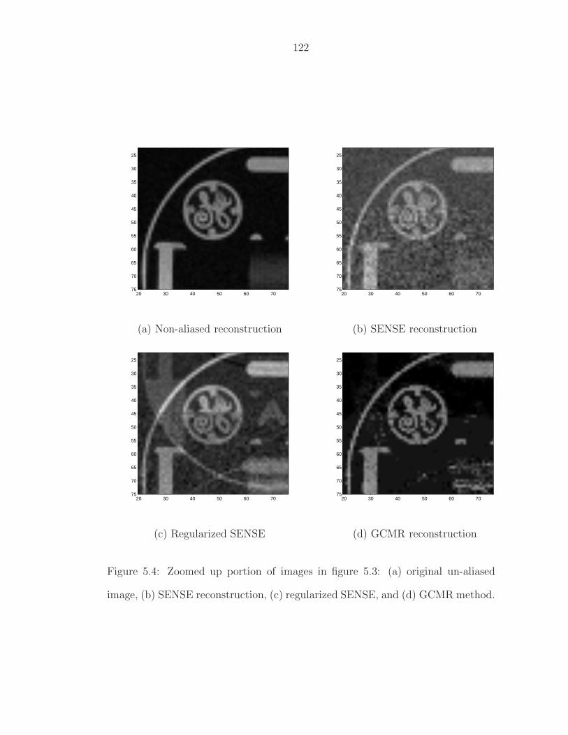
122

20 30 40 50 60 70

25

30

35

40

45

50

55

60

65

70

7520 30 40 50 60 70

25

30

35

40

45

50

55

60

65

70

75

(a) Non-aliased reconstruction (b) SENSE reconstruction

20 30 40 50 60 70

25

30

35

40

45

50

55

60

65

70

7520 30 40 50 60 70

25

30

35

40

45

50

55

60

65

70

75

(c) Regularized SENSE (d) GCMR reconstruction

Figure 5.4: Zoomed up portion of images in figure 5.3: (a) original un-aliased

image, (b) SENSE reconstruction, (c) regularized SENSE, and (d) GCMR method.

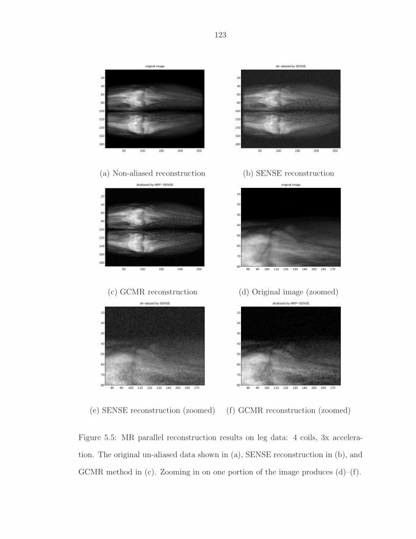
123

original image

50 100 150 200 250

20

40

60

80

100

120

140

160

180

de−aliased by SENSE

50 100 150 200 250

20

40

60

80

100

120

140

160

180

(a) Non-aliased reconstruction (b) SENSE reconstructiondealiased by MRF−SENSE

50 100 150 200 250

20

40

60

80

100

120

140

160

180

original image

80 90 100 110 120 130 140 150 160 170

10

20

30

40

50

60

70

80

(c) GCMR reconstruction (d) Original image (zoomed)de−aliased by SENSE

80 90 100 110 120 130 140 150 160 170

10

20

30

40

50

60

70

80

dealiased by MRF−SENSE

80 90 100 110 120 130 140 150 160 170

10

20

30

40

50

60

70

80

(e) SENSE reconstruction (zoomed) (f) GCMR reconstruction (zoomed)

Figure 5.5: MR parallel reconstruction results on leg data: 4 coils, 3x accelera-

tion. The original un-aliased data shown in (a), SENSE reconstruction in (b), and

GCMR method in (c). Zooming in on one portion of the image produces (d)–(f).

124

original image

50 100 150

120

130

140

150

160

170

180

de−aliased by SENSE

50 100 150

120

130

140

150

160

170

180

(a) Original image (zoomed) (b) SENSE reconstruction (zoomed)dealiased by MRF−SENSE

50 100 150

120

130

140

150

160

170

180

(c) GCMR reconstruction (zoomed)

Figure 5.6: Another zoomed portion of data presented in figure 5.5 (a), SENSE

reconstruction, (b)SENSE and (c) GCMR.

125

diffusion with our method on identical energy functions, much as [TF03] compared

LBP with graph cuts.

In the field of parallel MR reconstruction, a major extension would be to cover

other sampling trajectories like spiral or radial. These trajectories will in general

result in the entries of system matrix E being complex - a case that our current

method is unable to handle. A generalization to arbitrary matrices will remove

this restriction.

Chapter 6

Conclusions

This thesis described a number of algorithms related to the acquisition, recon-

struction and post-processing of Magnetic Resonance data. These algorithms form

parts of an elegant, unified linear systems framework within which fall many excit-

ing and challenging problems in MR. The unified systems approach was inspired by

developments in other computational fields like vision, signal and image processing.

There have been few and sporadic attempts at exploiting the developments in these

other fields for use in MRI, and this thesis should be considered a long-overdue

step in that direction. We have used various ideas from estimation and detection

theory, Graph Theory and multi-variate optimization and put them within the

overall linear systems framework for MR. The algorithms we presented have the

potential to result in disruptive innovations in several areas of MR. We argued

that these techniques address in different but complementary ways the common

goal of improving the fundamental time-quality trade-off in MR imaging. Let us

list some novel ideas contained in the thesis.

We developed a new retrospective motion correction technique based on suc-

cessive convex projections. The method corrects a motion corrupted frame in

MRA sequence by iteratively making it more similar to a non-corrupted one. The

algorithm is able to correct corrupted features both in k-space and image space

without degrading radiologically important temporal events. The technique has

the potential to retrieve corrupted angiography data that would otherwise be un-

usable due to motion artifacts. Results indicate significant improvement in MRA

126

127

quality, both from visual evidence as well as from a double-blind comparison.

A maximum-likelihood algorithm was developed to obtain an optimal solution

to the parallel imaging reconstruction problem in the presence of both measurement

and sensitivity noise. We argued that existing methods prove quite inadequate in

tackling this problem, which is in fact a more natural model of the parallel imaging

process than those used currently. We showed that for i.i.d. Gaussian noise the

optimal solution is the minimizer of a weakly non-quadratic objective function

which we solved efficiently via a non-linear least squares iterative technique with

modest additional complexity compared to standard SENSE algorithms. A fast

Newton algorithm with explicit Jacobian information was developed to solve the

problem. Results for Cartesian k-space sampling indicate impressive improvement

in performance compared to standard SENSE, amounting to almost 20 dB SNR

gain in several high-noise cases. The algorithm yields substantial improvement

even in cases where the i.i.d. Gaussian sensitivity noise model implicit in the

method is not accurate.

Next we developed a new graph cut method to solve Bayesian estimation prob-

lems that arise in medical imaging, signal and image processing and machine vision.

This approach benefits immensely from a Markov Random Field (MRF) based for-

mulation of a priori information. The main restriction of our technique is that it

works only on linear systems with non-negative matrix elements. We developed

the general case, then specialised it to image deconvolution, motion deblurring and

MR reconstruction from parallel data. The basic idea behind MRF-based Bayesian

estimation is to impose a discontinuity-preserving smoothness term, which we ac-

complished by assuming the prior to have a Gibbsian distribution defined on an

MRF. We developed a fast energy minimization method based on graph cuts to

128

solve this rather challenging numerical problem. We demonstrated our method by

applying it for image deconvolution and motion deblurring on real images, as well

as parallel MR reconstruction from raw Fourier data.

Taken separately or in combination with each other, the techniques presented

in this thesis form a promising foundation upon which to build a unified linear

systems approach to solving medical imaging problems.

6.1 Extensions

6.1.1 TL-SENSE for arbitrary sampling

The TL-SENSE algorithm developed in chapter 4 concentrated on the Cartesian

sampling case, which happens to be the most widely used method currently. How-

ever, in the future, other trajectories like spira lor radial are likely to become

very popular, since they intrinsically sample th emiddle of k-space, where most

of the data lies, more densely than outer k-space. Using these nearly-sphericaly-

symmetric trajectries is also very useful during motion correction. Hence a power-

ful extension of the TL-SENSE method would be to allowthe use of these trajec-

tories. The reconstruction can no longer be reduced to independent sub-problems

over columns like the Cartesian case, so the new algorithm is likely to be much

more computationally challenging. But a modified Conjugate Gradients approach

could perform reasonably well without incurring prohibitive compuation time.

6.1.2 TL-SENSE for general noise models

Recall that our algorithm assumes i.i.d. Gaussian noise in sensitivity maps. While

we presented some data to support our contention that the method does well even

129

when this assumption is violated, there is a case for an algorithm that can handle

arbitrary noise models. For instance, consider the situation where the sensitivity

errors are mainly due to mis-orientation of coils between actual scan and pre-scan.

Or the case where flexible receiver pads were used. Sensitivity noise in these cases

can not be easily modelled under the i.i.d. assumption, but it can be safely assumed

that such noise is of a low-frequency nature. We are currently exploring ways to

extend the TL-SENSE algorithm to these noise models. Preliminary results suggest

improvement upon the i.i.d. noise assumption, but much more work needs to be

done before we obtain a final algorithm.

6.1.3 Graph Cut methods for arbitrary linear systems

An obvious extension of our MRF based Bayesian work would be to generalize our

results to arbitrary linear systems, and not merely those with non-negative entries.

Among other things, this will prove useful for arbitrary sampling trajectories in

MR, as well as some deblurring problems (not frequently occurring however) in

images. A general algorithm will make the method useful for other linear systems

outside of vision or medical imaging.

BIBLIOGRAPHY

[AMH91] Theagenis J. Abatzoglou, Jerry M. Mendel, and Gail A. Harada. TheConstrained Total Least Squares technique and its applications toharmonic superresolution. IEEE Transactions on Signal Processing,39(5):1070–1087, May 1991.

[BB98] M Beretro and P Boccacci. Introduction to Inverse Problems inImaging. Institute of Physics Publishing, 1998.

[BS93] Charles Bouman and Ken Sauer. A generalized Gaussian imagemodel for edge preserving MAP estimation. IEEE Transactions onImage Processing, 2(3):296–310, July 1993.

[BVZ01] Yuri Boykov, Olga Veksler, and Ramin Zabih. Fast approximateenergy minimization via graph cuts. IEEE Transactions on Pat-tern Analysis and Machine Intelligence, 23(11):1222–1239, Novem-ber 2001.

[DEMM03] McRobbie DW, Moore EA, Graves MJ, and Prince MR. MRI: FromPicture to Proton. Cambridge, UK, 2003.

[ea96] R. Zoroofi et al. Cancellation of MRI artifacts in image plane. IEEETransactions on Medical Imaging, 5(6):178–182, June 1996.

[EK02] N. Park et al E. Kim. Cancellation of MRI motion artifact in imageplane. IEEE I&M Technical Conference Proceedings, pages 329–334,May 2002.

[Fer94] P. J. Ferreira. Interpolation and the discrete Gerchberg-Papoulisalgorithm. IEEE Transactions on Signal Processing, 42(10):22–29,October 1994.

[FL97] Mario A. Figueiredo and Jose M. Leitao. Unsupervised imagerestoration and edge location using compound Gauss-Markov ran-dom fields and the MDL principle. IEEE Transactions on ImageProcessing, 6(8):1089–1102, August 1997.

[GBD04] P. Gravel, G. Beaudoin, and J.A. DeGuise. A method for modelingnoise in medical images. IEEE Transactions on Medical Imaging,23(10):1221–1232, October 2004.

[GL96] G. Golub and C. Van Loan. Matrix Computations. Johns HopkinsUniversity Press, 1996.

[GPR67] L G Gubin, B T Polyak, and E V Raik. The method of projectionsfor finding the common point of convex sets. USSR ComputationalMathematics and Mathematical Physics, 7:1–24, 1967.

130

131

[GWB86] E. Gmelin, H. D. Weiss, and F. Buchmann. Cardiac gating in intra-venous dsa. European J. Radiology, 6(1):24–29, 1986.

[HL02] Sabine Van Huffel and Philippe Lemmerling. Total Least Squaresand Errors-in-Variables Modeling: Analysis, Algorithms and Appli-cations. Kluwer, 2002.

[Hog03] W. S. Hoge. A subspace identification extension to the phase corre-lation method. IEEE Transactions on Medical Imaging, 22(2):223–227, February 2003.

[Ish03] Hiroshi Ishikawa. Exact optimization for Markov Random Fieldswith convex priors. IEEE Transactions on Pattern Analysis andMachine Intelligence, 25(10):1333–1336, October 2003.

[Kay93] S. Kay. Fundamentals of Statistical Signal Processing: Volume I -Estimation Theory. Prentice-Hall, Upper Saddle River, NJ, 1993.

[Kim03] Junwan Kim. Computer Vision Algorithms in Magnetic ResonanceImaging. PhD thesis, Cornell University, August 2003.

[KPZ+02] Junhwan Kim, Martin R. Prince, Ramin Zabih, Jeff Bezanson,Richard Watts, Hale E. Erel, and Yi Wang. Automatic selec-tion of mask and arterial phase images for temporally-resolved mrdigital subtraction angiography. Magnetic Resonance in Medicine,48(6):1004–1010, 2002.

[KZ03] Junhwan Kim and Ramin Zabih. Automatic segmentation ofcontrast-enhanced image sequences. In International Conference onComputer Vision, pages 502–509, 2003.

[KZ04] Vladimir Kolmogorov and Ramin Zabih. What energy functionscan be minimized via graph cuts? IEEE Transactions on PatternAnalysis and Machine Intelligence, 26(2):147–159, February 2004.

[LBJ+02] Z. P. Liang, R. Bammer, J. Ji, N. Pelc, and G. Glover. Improvedimage reconstruction from sensitivity-encoded data by wavelet de-noising and Tikhonov regularization. In Proc. International SummerSchool on Biomedical Imaging, pages 493–496, 2002.

[LdMH96] Philippe Lemmerling, Bart de Moor, and Sabine Van Huffel. Onthe equivalence of Constrained Total Least Squares and StructuredTotal Least Squares. IEEE Transactions on Signal Processing,44:2908–2911, November 1996.

[Li95] S. Li. Markov Random Field Modeling in Computer Vision.Springer-Verlag, 1995.

132

[LL99] Zhi-Pei Liang and Paul C Lauterbur. Principles of Magnetic Reso-nance Imaging: A Signal Processing Perspective. IEEE Press, 1999.

[MGK95] Vladimir Z. Mesarovic, Nikolas P. Galatsanos, and Aggelos K.Katsaggelos. Regularized Constrained Total Least Squares imagerestoration. IEEE Transactions on Image Processing, 4(8):1096–1108, August 1995.

[MNV99] Erik H. Meijering, Wiro J. Niessen, and Max A. Viergever. Ret-rospective motion correction in digital subtraction angiography: Areview. IEEE Transactions on Medical Imaging, 18(1):2–21, January1999.

[MOY+01] C. A. McKenzie, M. A. Ohliger, E. N. Yeh, M. D. Price, and D. K.Sodickson. Coil-by-coil image reconstruction with SMASH. Mag-netic Resonance in Medicine, 46:619–623, 2001.

[MP03] K. L. Miller and J. M. Pauly. Nonlinear phase correction for navi-gated diffusion imaging. Magnetic Resonance in Medicine, 50:343–353, 2003.

[MTJ98] Prince MR, Grist TM, and Debatin JF. 3D Contrast MR Angiog-raphy. Springer-Verlag, New York, 1998.

[OFS88] P Oskoui-Fard and H Stark. Tomographic image reconstructionusing convex projections. IEEE Transactions on Medical Imaging,7:45–58, March 1988.

[Opi67] Z. Opial. Weak convergence of the sequence of successive approxi-mations for nonexpansive mappings. Bulletin of the American Math-ematical Society, 73:591–597, 1967.

[Pea88] Judeah Pearl. Probabilistic reasoning in intelligent systems: net-works of plausible inference. Morgan Kaufmann, 1988.

[PM90] P. Perona and J. Malik. Scale space and edge detection usinganisotropic diffusion. IEEE Transactions on Pattern Analysis andMachine Intelligence, 12(7):629–639, July 1990.

[PT97] Yani Picard and Christopher J. Thompson. Motion correction ofpet images using multiple acquisition frames. IEEE Transactionson Medical Imaging, 16(2):137–144, April 1997.

[PTK85] Tomaso Poggio, Vincent Torre, and Christof Koch. Computationalvision and regularization theory. Nature, 317:314–319, 1985.

[PTVF92] William Press, Saul Teukolsky, William Vetterling, and Brian Flan-nery. Numerical Recipes in C. Cambridge, 2nd edition, 1992.

133

[PWBB01] K. P. Pruessmann, M. Weiger, Peter Boernert, and Peter Boesiger.Advances in sensitivity encoding with arbitrary k-space trajectories.Magnetic Resonance in Medicine, 46:638–651, 2001.

[PWSB01] K. P. Pruessmann, M. Weiger, M. B. Scheidegger, and Peter Boe-siger. SENSE: sensitivity encoding for fast MRI. Magnetic Reso-nance in Medicine, 42(5):952–962, 2001.

[RA98] K. Ratakonda and N. Ahuja. POCS-based adaptive image magnifi-cation. Proceedings, International Conference on Image Processing,pages 1231–35, October 1998.

[SM97] P. Stoica and R. L. Moses. Introduction to Spectral Analysis.Prentice-Hall, 1997.

[SS02] Daniel Scharstein and Richard Szeliski. A taxonomy and evaluationof dense two-frame stereo correspondence algorithms. InternationalJournal of Computer Vision, 47:7–42, April 2002.

[TF03] M.F. Tappen and W.T. Freeman. Comparison of graph cuts withbelief propagation for stereo, using identical MRF parameters. InInternational Conference on Computer Vision, pages 900–907, 2003.

[TM98] C. Tomasi and R. Manduchi. Bilateral filtering for gray and colorimages. In International Conference on Computer Vision, pages839–846, 1998.

[TRF04] M.F. Tappen, B.C. Russell, and W.T. Freeman. Efficient graphicalmodels for processing images. In IEEE Conference on ComputerVision and Pattern Recognition, pages II: 673–680, 2004.

[vdBWK+03] Johan S. van den Brinka, Yuji Watanabeb, Christiane K. Kuhlc,Taylor Chungd, Raja Muthupillaia, Marc Van Cauterena, Kei Ya-madae, Steven Dymarkowskif, Jan Bogaertf, Jeff H. Makig, CelsoMatosh, Jan W. Casselmani, and Romhild M. Hoogeveena. Impli-cations of SENSE MR in routine clinical practice. European Journalof Radiology, 46(1):3–27, April 2003.

[WBP04] Florian Wiesinger, Peter Boesiger, and Klaas Pruessmann. Elec-trodynamics and ultimate SNR in parallel MR imaging. MagneticResonance in Medicine, 52(2):376–390, August 2004.

[Wel67] P. D. Welch. The use of fast fourier tranforms for the estimationof power spectra: A method based on time averaging over shortmodified periodograms. 15:70–73, 1967.

134

[WND+03] B. J. Wintersperger, K. Nikolaou, O. Dietrich, J. Rieber, M. Nittka,M. F. Reiser, and S. O. Schoenberg. Single breath-hold real-timecine MR imaging: improved temporal resolution using generalizedautocalibrating partially parallel acquisition (GRAPPA) algorithm.European Journal of Radiology, 13(8):1931–1936, May 2003.

[XH01] Yingbiao Xu and E M Haacke. Partial fourier imaging in multi-dimensions: A means to save a full factor of two in time. 14:628–635,2001.