Improvement of Machine Tool Movements for Simultaneous Five-Axes Milling

A. Zabel1, H. Müller

2, M. Stautner

1, P. Kersting

1

1 Department of Machining Technology, University of Dortmund, Germany 2 Department of Computer Graphics, University of Dortmund, Germany

Abstract Generating five-axes NC-paths by a standard CAM-system still contains many problems, especially concerning the simultaneous movements of all axes of a given machine tool. These movements are often not smooth enough and lead to unwanted jerks resulting in a poor quality of the workpiece surface. In order to reduce this effect, two different algorithms are introduced in this paper. First approaches of optimising the machine kinematics by using a standard evolution strategy are presented as well as the integration of these algorithms in a simulation environment for five-axes milling processes.

Keywords: Five-Axes Milling, Kinematic Optimisation, Evolution Strategy, Wavelets

1 INTRODUCTION

In contrast to three-axes milling, the NC-path generation for five-axes processes cannot be considered to be state of the art, especially in the case that complex free-formed surfaces have to be machined. Today NC-paths are usually programmed by a standard CAM-system. These tool paths are often not satisfactory, especially concerning the simultaneous movements of all machine tool axes. Being usually not smooth enough these movements lead to undesirable jerky motion changes which result in a deficient quality of the workpiece surface.

In order to improve this situation, different algorithms have been applied and integrated in a simulation environment for five-axes milling processes. The simulation is placed in the process chain between the CAM-system and the real milling process, and calculates the complete material removal process during milling in an efficient and exact manner. Additionally, the simulation system models the machine tools axes configuration and its dynamic behaviour. The main input are NC-paths, generated by a CAM-system. Additional information concerning the raw stock material and a specification of the milling tool has to be provided by the user.

During the virtual milling process, the input NC-paths are analysed and optimisations can be calculated. A first algorithm for smoothing the movements of the milling tool is working as linear filter. For that purpose, the angles between short segments of the guiding curves for the milling tool are considered. Another more complex approach computes path optimisations based on an evolutionary algorithm (EA). The EA works on a wavelet transformation of the NC-path’s tilt and roll angles and optimises the coefficients of the wavelet functions. Both approaches lead to smooth and jerk-free paths and they improve surface quality of a given workpiece. The optimisations calculated by the algorithms are always carried out under the constraint that the generated tool path should be collision-free and technologically well suited. Therefore, an efficient collision detection engine also plays an important role in the presented approach.

Several approaches to NC-path optimisation with different optimisation objectives have been published in the past. Yoon evaluates optimal cutting positions of a flat or toroidal endmill with respect to the avoidance of tool tip gouging [1]. My at el. [2] introduced an approach for 5-axis tool path optimisation by clustering the optimal cutting direction vector field. Stautner and Zabel [3] have developed a prototype of a semi-automatic optimisation

system which uses evolutionary algorithms to optimise multi-axis tool paths with regard to cutting force reduction and collision prevention. Surmann, Kalveram and Weinert [4] have introduced a simulation system which predicts the vibration behaviour of the cutting tool along arbitrary NC programs for the milling of sculptured surfaces. This software allows the prediction of those segments of an NC-program which are sensitive to chattering vibrations. Their objective is the adaptation of the process parameters using this knowledge. Analysis of research literature shows that the influence of the kinematics of machine elements has not been taken into account by now.

The paper starts with an introduction into the overall milling and kinematic simulation (section 2 and section 3) and its collision detection. In section 4, the algorithms used for the kinematic optimisation are presented as well as their integration into the simulation. Results of both algorithms are presented and discussed in section 5.

Figure 1: Schematic dexel field representation. Left/ Middle: single dexel field without/ with undercuts. Right: a

workpiece consisting of three dexel fields.

2 MILLING SIMULATION

The primary objective of a milling simulation is the imitation of the real milling process behaviour in order to gain insight into the system operation, to detect optimised process parameters, for example for achieving higher product quality and saving costs and time without any risk of collision or of tool breakage, and to translate the simulation results to the real process. Therefore, simulating requires a representation of the relevant characteristics as detailed and realistic as possible. The choice of model for the workpiece and milling tool influences the precision and the running time of the simulation, and therewith depends on the different fields of application [6].

y

x

z

Intelligent Computation in Manufacturing Engineering - 5

Modelling a workpiece for five-axis milling, several requirements have to be regarded, especially the support of undercuts in tolerable precision and running time. In the following, a prototype of a milling simulation is used which depends on a special discrete workpiece representation (dexel field, see Figure 1) and a CSG (Constructive Solid Geometry [5])-based model for the milling tool (Figure 2) as described in [5, 6].

Figure 2: CSG modelled cutter.

3 KINEMATIC SIMULATION

As branch of mechanics, kinematics is concerned with the object motions without taking the forces into account that cause the movement. Depending on their constructive design, the milling machines can be divided into the group of serial and the group of parallel kinematic machines. The actual arrangement of rigid members and joints of a serial kinematic machine is like a chain, whereas parallel kinematic machines are based on a closed-loop mechanism in which the end-effector is connected to the base by at least two independent kinematic chains [8]. This article is focussed on a special parallel kinematic machine (Mikromat 6X Hexa [9]) which is shown in Figure 3. For simulation, the kinematic elements of the milling machine are modelled by triangle meshes.

Figure 3: Extract of the parallel kinematic simulation.

An important objective of kinematic simulation is the detection of collisions between moving machine parts, and the possibility to correct the NC-path before executing the real milling process.

In literature, several algorithms and libraries for collision detection are known [10]. Because the machine parts are modelled by triangle meshes in the introduced simulation prototype, the library VCollide developed by Hudson et al. [11] was chosen. The main idea of VCollide is to use a hierarchical approach in order to find colliding pairs of objects. In a first step, potential colliding pairs are searched, using an n-body sweep-and-prune algorithm on axis-aligned bounding boxes (see [12]). On the next level, collisions are detected based on a hierarchy of oriented bounding boxes (OBB for short) for every object.

The root of the bounding box tree contains the box including the entire object; the leaves contain only one or very few primitives (triangles). Checking for collisions between a pair of objects, their OBB hierarchies are descended in order to find leaves which overlap. In this case, an exact intersection test between the triangles in the overlapping leaves is performed [11].

Using this algorithm in the simulation prototype, the current positions and orientations of the milling machine parts have to be calculated from the active location of the tool centre point and have to be transferred to the VCollide algorithm. The process of calculating the location of the linked structure from the given endpoint (equivalent to the tool centre point in this case) is known as inverse kinematic transformation [9]. In order to calculate the new positions and orientations, the simulation needs a mathematical description of the movement behaviour of every single machine part and information about the way the individual parts are joined.

4 IMPROVEMENT OF MACHINE TOOL MOVEMENTS

The movements of kinematic elements can influence the surface quality. In particular, jerky motion changes of heavy machine components, for example the spindle holder, could result in oscillations and therewith in surface defects on the workpiece (Figure 4).

Figure 4: Extraction of a real workpiece. A/B: surface defects resulting from vibrations of machine elements.

This motivates to analyse and to modify the motion path of individual kinematic elements in order to get an improved surface quality. The idea is to leave the position of the tool centre point unchanged, but allowing the modification of the tilt and roll angles. In this context, it is taken as a useful precondition that modifying the tool angles of ball cutters does not influence the milling result as long as the radial part of the cutting edge is in engagement.

During the combined milling and kinematic simulation of a given NC-path, the angle functions and motion curves of selected machine elements are recorded. The idea is to smooth these angle functions with the restriction of maintaining its principal characteristics and the limitation of considering the quality of the motion curves of a machine element. For that purpose, two different approaches are introduced in the following: a first one, working as linear filter and a second, more complex one based on an evolutionary algorithm.

4.1 Linear Approximation Algorithm

The linear approach is based on the Iri-Imai-Algorithm which was introduced in 1986 by I. Iri and H. Imai [13]. The main idea is to smooth the input curve C consisting of n points P1, …, Pn by reducing the number of points using the following instruction: all points Pk lying between

A

B

two points Pi and Pj could potentially be deleted if the distance between each point Pk and the line PiPj is smaller than a given tolerance ε (see Figure 5).

Figure 5: Tolerance illustration. a) Because the point Pk is located outside the tolerance field, Pi and Pj may not be

connected. b) Enlarging ε legalises this connection.

In order to calculate a smoothed curve C’, a directed graph has to be generated which includes the points of the initial curve C as nodes. Two graph nodes are connected with an edge if PiPj satisfies the given tolerance. Every edge gets a weight indicating how many points Pk could be eliminated from the original curve if the connection between Pi and Pj is admitted. Afterwards, the path C’ from P1 to Pn with maximal weightings is detected.

Due to the linearity of the algorithm, the generated curve still contains more or less sharp edges. In order to correct this effect, the algorithm is applied iteratively with exceeding tolerances until the resulting curve is satisfying. Another possibility is to use a post-processing process in order to smooth the curve, for example by using Hermite interpolation [21]. Examples will be presented and discussed in section 5.

Figure 6: Algorithm overview.

4.2 Wavelet Based Smoothing Algorithm

Because of the linearity of the introduced approximation algorithm, a second approach is now presented which is more complex and combines three general principles: the wavelet transform in order to achieve a representation of the angle functions suitable to optimisation, curve features to express the objectives, and evolutionary

strategies for optimising the angle function. A schematic overview of the algorithm is shown in Figure 6; a more detailed description is given in the following.

The use of evolutionary algorithms is reasonable in this context because the correlation between the variable components is quite complex. In order to reduce the high number of degrees of freedom which is critical for the application of evolution strategies, a matrix splitting approach is used.

Wavelet transform

The following brief introduction of the wavelet transform is limited to those aspects being relevant for this article. Further information can be found in literature [13, 14, 15]. Like the classical Fourier transform [17], the wavelet transform represents a given function as a linear combination of a set of basis functions. In contrast to the Fourier transform, where infinite sine and cosine functions are used, the wavelet functions are usually equal to 0 outside a finite interval and in this way suited for local analysis of restricted regions of interest.

The basis functions of a wavelet transform are distinguished in two groups: the scaling functions and the wavelet functions – or just wavelets for short. While the former type is used to represent a crude approximation of the function, the wavelets represent details of different resolution or frequency. To simplify matters, the scaling functions are omitted and only the wavelets are specified in the following.

The wavelet functions j ,kψ are obtained from a basis ψ

– called mother wavelet (Figure 7) – by dilatation and translation,

2( ) 2 (2 ) ( )j jj,kψ t ψ t k , j,k .= − ∈� (1)

In this context, the functions to be optimised are the sampled angle values at discrete time locations 0, …, n-1. Therefore, the discrete wavelet transform is required which represents a function f(t), t=0, …., n-1, in the following representation form (n=2

m):

1 2 1

0 0

( ) ( ) ( )

jm

0,0 0,0 j,k j,k

j k

f t c φ t d ψ t .

− −

= =

= +∑ ∑ (2)

0,0φ is a scaling function with the scaling coefficient

0,0c .∈� j,kd ∈� are the wavelet coefficients. Thereby,

the number of (scaling and wavelet) coefficients after the transformation is equivalent to the number of input values. The explicit function f(t) can be recalculated from the coefficients of the wavelet transform by the inverted discrete wavelet transform. Efficient algorithms are available for the discrete wavelet transform and the inverted transform as well [16].

Figure 7: Examples of mother wavelets.

Accentuating the influence of the coefficients and their corresponding wavelets on the input function f(t), an intuitive graphical arrangement of the wavelet coefficients

is used, which is shown in Figure 8 for a very small example of 32 data values; in real applications several thousand values are usual. The domain of the given function is represented by the horizontal axis and the level of frequency by the vertical one. This means that the first row contains the coefficient belonging to the function with the largest dilatation, whereas the coefficients corresponding to fine details are located in the last row. Relating to the input function, the largest dilatation has influence on the whole data set, whereas the other coefficients affect just intervals of decreasing length.

Figure 8: Arrangement of wavelet coefficients.

Wavelet based optimisation

The idea of optimising the curve function is to transform the angle values into a wavelet representation and to adjust the corresponding wavelet coefficients before applying the inverse transform (Figure 6). Therefore, a classical evolution strategy is used [17, 18] working on a population of potential solutions – called individuals – and manipulating these individuals with evolutionary operators [20]. In this context, each individual consists of a complete set of wavelet coefficients initialised with the coefficients belonging to the input functions. Furthermore, the (µ+λ)-strategy is applied for avoiding curves with worse progression.

In addition to the mutation and recombination operators, an additional modification – known as wavelet shrinkage [16] – is used which reduces all coefficients smaller than a given threshold value to 0. In this way, the functions get more or less smoothed, dependent on the threshold magnitude.

Since it is more convenient to evaluate angle functions in explicit representation than the wavelet coefficients themselves, an inverse wavelet transform is applied to every individual before evaluating the fitness function. After inverse transformation, the kinematic simulation is started, and new motion curves of relevant kinematic elements are recorded. Afterwards, the weighting function is evaluated for each individual and the characteristics of the angle functions are comprised as well as the motion curves. The best µ individuals are chosen for creating the next generation’s population.

Fitness Function

For quantifying the optimality of a solution (individual) several features of the functions seen as curves are used: the curvature, the length, and the deviation of the modified curve from the original one.

Curvature is chosen as important criterion of curve behaviour because sharp bends in a motion curve mean strong motion changes. Thus, curves of small curvature are preferred. In order to evaluate the curvature, the sum

of absolute cosines of the angles iω between two

adjacent curve segments PiPi+1 and Pi+1Pi+2 are used:

+1 +2 +1

+1 +2 +1=1 =1

n ni i i i

ii i i ii i

P P ,P Pcos ,

P P P Pκ ω

− −

= =

− −∑ ∑ (3)

where Pi are the angle values at the i-th simulation step. To avoid wavy curve results, the curve length is used as another important feature which is calculated from the average sum of Euclidean distances d:

+1

=1

1( )

n

i i

i

l d P , P .n

= ∑ (4)

Taking just curvature and curve length as features into account, the optimisation would always result in a straight line – independently of the shape of the original curve. This effect is not desired, because the angles would not change during the process, and thus, two of the five available degrees of freedom (three along the coordinate axes and two angles) would not be used. For this reason, the deviation from the original curve is chosen as another important criterion, which is evaluated as squared Euclidean distance between the points of the original curve Pi

orig and the ones of the modified curve Pimod:

2

=1

1( )

norig mod

ii

i

a d P , P .n

= ∑ (5)

Providing the different features (curvature κ , curve length l and deviation a from the original curve) with individual weights, the complete evaluation e of a curve

can be calculated as κ l ae g κ g l g a,= + + where κg ∈�

is the weight of curvature κ , lg ∈� the weight of curve

length and ag ∈� the weight of deviation.

For evaluating the complete fitness function the evaluations of the tool attack angles themselves as well as the ones of the motion curves of selected relevant machine components have to be involved:

=1

( )

mκ l a

j j j j

j

q g g κ g l g a ,= + +∑ (7)

where the index j indicates the curve and jg ∈� is the

weight of the j-th curve.

Figure 9: Generating submatrices.

Managing the data

In real applications, several thousand recorded data values are usual which result in the same high number of wavelet coefficients after transformation. Being the input

for the optimisation algorithm, these many of coefficients cause a high number of degrees of freedom which is very critical for the application of evolution strategies. To handle this problem, a technique based on the observation that sharp bends in a curve are reflected in large wavelet coefficient values, has been developed. This feature allows smoothing the curve without modifying any of the values, but just the large ones and those in the neighbourhood of large coefficients. Using this effect, the optimisation of the complete data set can be divided in several smaller optimisation problems around interesting wavelet coefficient values. For the following explanation, the kind of coefficient notation introduced above is used.

Figure 10: Schematic overview of the splitting approach. (*) Regarding the process runtime, only the generated

submatrices (1) are involved into the modifying process, the complete matrix (2) has been retained unchanged.

Scanning the matrix for interesting (large) coefficient values in the bottom row and creating submatrices of constant size consisting of 14 coefficients, is the main idea of this approach. The submatrices are extracted from the complete structure by resetting its coefficients to zero (Figure 9). The inverse wavelet transform is applied to this modified complete matrix, whereas each of the small submatrices is optimised separately by a standard evolution strategy before it is also inversely transformed. Due to the linearity of the wavelet transform [14] the complete and optimised result is obtained by adding the separate inverse transformed modified matrix and the transformed optimised submatrices.

Obviously, splitting the large-sized problem of optimising the complete set of several thousand recorded data values into problems of a smaller number of degrees of

freedom, the optimisation problem gets manageable and the performance of the algorithm is improved. A short schematic process overview is given in Figure 10.

Collision handling

After generating a new NC-path with respect to the optimised angles, a collision test is necessary. Therefore, the new generated tool path is simulated again and detected collisions are eliminated.

Due to the assumption that the original NC-path causes no incidents, the collisions detected by the simulation of the new generated tool path can be treated by using the original data in the environment of critical locations. In order to achieve a smooth fading from the modified to the original curve, a kind of Hermite interpolation [21] is used. As long as the NC-path is modified, the process of simulation, collision detection and correction has to be repeated to be sure to get legal and collision free tool paths.

5 EXAMPLES AND RESULTS

With respect to the objective of milling process optimisation, results of both introduced algorithms are presented and discussed in the following explanations.

At first, a drafted example of linear data optimisation is depicted in Figure 11. Figure 11(a) shows the raw data. In order to avoid a high tolerance value ε, additional data values (white dots in Figure 11(b)) are inserted at long edges. The algorithm is iteratively applied (Figure 11(c)-(d)) resulting in the interpolation shown in Figure 11(e). A relation of the raw data (continuous curve) and the resulting curve (dotted line) is represented in Figure 11(f). The result of the linear approach depends on the choice of the tolerance ε. Too large values of ε results in a straight line, whereas too small ones have no effects. Using additional data values (white dots in Figure 11(b)) results in acceptable angle curves. In the introduced example increasing ε values (ε =0.8, 0.7, … 0.2) were used. The remarkable disadvantage of this approach is the linearity which enforces a post processing editing.

Figure 11: Illustration of the linear optimisation approach.

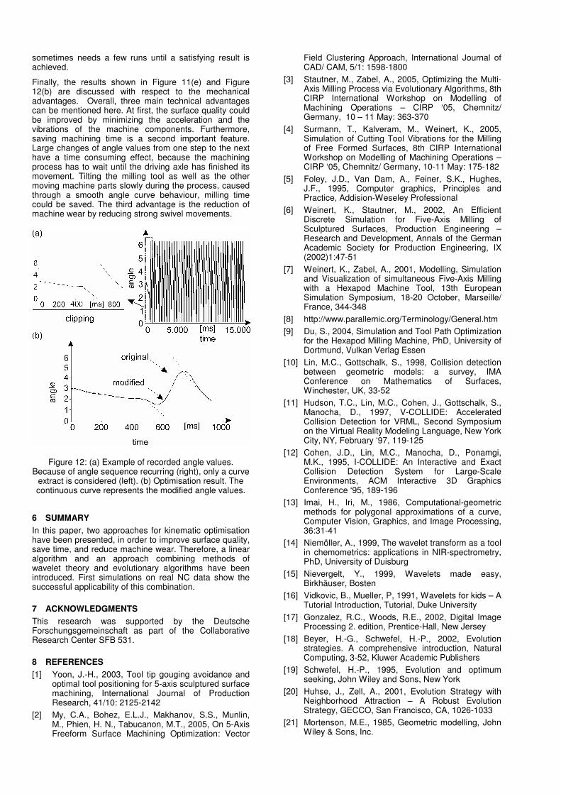
For the purpose of validating the introduced wavelet based approach, the machining of a test workpiece (Figure 4) has been simulated and the required angle data has been recorded. An example of the recorded values is shown in Figure 12(a). The wavelet-based algorithm has been applied with the following adjustments: a (5, 10)-standard evolution strategy with a restricted number of cycles was used and the weights were chosen in a ration of 5:1:3 (length: curvature: deviation). The result (continuous curve) is shown in Figure 12b. Obviously, the sharp bends of the original curve are smoothed, while the mean characteristics of the raw data are kept.

Comparing the introduced approaches, both algorithms offer advantages and disadvantages. In the case of the wavelet-based approach, there is no need of a post- processing. The linear algorithm generates dependably well modelled results, whereas the evolutionary approach

sometimes needs a few runs until a satisfying result is achieved.

Finally, the results shown in Figure 11(e) and Figure 12(b) are discussed with respect to the mechanical advantages. Overall, three main technical advantages can be mentioned here. At first, the surface quality could be improved by minimizing the acceleration and the vibrations of the machine components. Furthermore, saving machining time is a second important feature. Large changes of angle values from one step to the next have a time consuming effect, because the machining process has to wait until the driving axle has finished its movement. Tilting the milling tool as well as the other moving machine parts slowly during the process, caused through a smooth angle curve behaviour, milling time could be saved. The third advantage is the reduction of machine wear by reducing strong swivel movements.

Figure 12: (a) Example of recorded angle values. Because of angle sequence recurring (right), only a curve

extract is considered (left). (b) Optimisation result. The continuous curve represents the modified angle values.

6 SUMMARY

In this paper, two approaches for kinematic optimisation have been presented, in order to improve surface quality, save time, and reduce machine wear. Therefore, a linear algorithm and an approach combining methods of wavelet theory and evolutionary algorithms have been introduced. First simulations on real NC data show the successful applicability of this combination.

7 ACKNOWLEDGMENTS

This research was supported by the Deutsche Forschungsgemeinschaft as part of the Collaborative Research Center SFB 531.

8 REFERENCES

[1] Yoon, J.-H., 2003, Tool tip gouging avoidance and optimal tool positioning for 5-axis sculptured surface machining, International Journal of Production Research, 41/10: 2125-2142

[2] My, C.A., Bohez, E.L.J., Makhanov, S.S., Munlin, M., Phien, H. N., Tabucanon, M.T., 2005, On 5-Axis Freeform Surface Machining Optimization: Vector

Field Clustering Approach, International Journal of CAD/ CAM, 5/1: 1598-1800

[3] Stautner, M., Zabel, A., 2005, Optimizing the Multi-Axis Milling Process via Evolutionary Algorithms, 8th CIRP International Workshop on Modelling of Machining Operations – CIRP ‘05, Chemnitz/ Germany, 10 – 11 May: 363-370

[4] Surmann, T., Kalveram, M., Weinert, K., 2005, Simulation of Cutting Tool Vibrations for the Milling of Free Formed Surfaces, 8th CIRP International Workshop on Modelling of Machining Operations – CIRP ‘05, Chemnitz/ Germany, 10-11 May: 175-182

[5] Foley, J.D., Van Dam, A., Feiner, S.K., Hughes, J.F., 1995, Computer graphics, Principles and Practice, Addision-Weseley Professional

[6] Weinert, K., Stautner, M., 2002, An Efficient Discrete Simulation for Five-Axis Milling of Sculptured Surfaces, Production Engineering – Research and Development, Annals of the German Academic Society for Production Engineering, IX (2002)1:47-51

[7] Weinert, K., Zabel, A., 2001, Modelling, Simulation and Visualization of simultaneous Five-Axis Milling with a Hexapod Machine Tool, 13th European Simulation Symposium, 18-20 October, Marseille/ France, 344-348

[8] http://www.parallemic.org/Terminology/General.htm

[9] Du, S., 2004, Simulation and Tool Path Optimization for the Hexapod Milling Machine, PhD, University of Dortmund, Vulkan Verlag Essen

[10] Lin, M.C., Gottschalk, S., 1998, Collision detection between geometric models: a survey, IMA Conference on Mathematics of Surfaces, Winchester, UK, 33-52

[11] Hudson, T.C., Lin, M.C., Cohen, J., Gottschalk, S., Manocha, D., 1997, V-COLLIDE: Accelerated Collision Detection for VRML, Second Symposium on the Virtual Reality Modeling Language, New York City, NY, February ‘97, 119-125

[12] Cohen, J.D., Lin, M.C., Manocha, D., Ponamgi, M.K., 1995, I-COLLIDE: An Interactive and Exact Collision Detection System for Large-Scale Environments, ACM Interactive 3D Graphics Conference ‘95, 189-196

[13] Imai, H., Iri, M., 1986, Computational-geometric methods for polygonal approximations of a curve, Computer Vision, Graphics, and Image Processing, 36:31-41

[14] Niemöller, A., 1999, The wavelet transform as a tool in chemometrics: applications in NIR-spectrometry, PhD, University of Duisburg

[15] Nievergelt, Y., 1999, Wavelets made easy, Birkhäuser, Bosten

[16] Vidkovic, B., Mueller, P, 1991, Wavelets for kids – A Tutorial Introduction, Tutorial, Duke University

[17] Gonzalez, R.C., Woods, R.E., 2002, Digital Image Processing 2. edition, Prentice-Hall, New Jersey

[18] Beyer, H.-G., Schwefel, H.-P., 2002, Evolution strategies. A comprehensive introduction, Natural Computing, 3-52, Kluwer Academic Publishers

[19] Schwefel, H.-P., 1995, Evolution and optimum seeking, John Wiley and Sons, New York

[20] Huhse, J., Zell, A., 2001, Evolution Strategy with Neighborhood Attraction – A Robust Evolution Strategy, GECCO, San Francisco, CA, 1026-1033

[21] Mortenson, M.E., 1985, Geometric modelling, John Wiley & Sons, Inc.