improvement of weka, a datamining tool
TRANSCRIPT

Spain:
Universidad Politecnica de Catalunya
Facultat Informatica de Barcelona
Belgium:
Universiteit Gent
Toegepaste Wetenschappen
Improvement of Weka, a datamining tool
by
Joachim Naudts
Spanish Promoter: Gavalda Mestre, Ricard
Belgian Promoter: Prof. dr.ir. G. Hoffman
year: 2003–2004

1

2
Copyright notice
“ The author grants the permission to make this thesis available for consultation and to copy
parts of it for personal use.
All other use is subjected to copyright laws, specifically to the obligation to explicitly mention
the source of quoted material. “
Joachim Naudts, June 2004

3
Preface
First of all, I would like to thank Ricard for the assistance and the tremendous amount of work
he did to guide this project to what it has become. Without his aid the result wouldn’t be nearly
as ’finished’ as it is now. Language barriers were non-existent and I enjoyed the collaboration a
lot.
Second I would like to thank all my friends and family, both in Barcelona and in Belgium. They
were always ready for the essential relaxations during this thesis. Especially I want to mention
Raf and Bruno, for the help and occasional discussions about this project.
Without my parents this thesis, but also this Erasmus year, would have been impossible. I
would like to thank them with all my heart for this wonderful opportunity and experience,
which probably changed me for the rest of my life.
Last but not least, I would like to thank Stefanie, for her great support. Even in difficult times,
she was always ready to listen or help in any possible way.
Joachim Naudts, June 2004

4
Improvement of Weka, a datamining toolby
Joachim Naudts
Year 2003–2004
Promoter: Gavalda Mestre, RicardFaculty: FIB
University: Universidad Politecnica de Catalunya
Research group: LSI
Overview
Weka (Waikato Environment for Knowledge Analysis) is a Machine Learning tool written inJava. It has a few hundred algorithms to perform all kinds of Data Mining tasks such asClassification, Clustering and Association. Weka is developed at the University of Waikato inNew Zealand. It was first mentioned in ”Data Mining: Practical Machine Learning Tools andTechniques with Java Implementations” [1].
However, Weka has one disadvantage: it can only handle small datasets. Whenever a set isbigger than a few megabytes an OutOfMemory error occurs. The object of this thesis is to alterWeka in such a way that it can handle ”all” datasets, up until a few gigabytes.
The first part of this thesis consists of designing and implementing some new classes that permita dataset to remain on disk. Of course this will have some drawbacks. The main, but inevitable,problem will be the decrease in performance.
The only solution for this problem is to use more intelligent algorithms. Those algorithms willbe based on sampling: a sample of the dataset is used so that the final result approximates theresult that would be obtained by running the non-sampling algorithm.
The second part will consist of implementing two of those sampling algorithms. The design ofthese algorithms is the responsibility of the director of this thesis (R. Gavalda). Implementationsare given for Sample K-Means, which is a clustering algorithm, and Sample Naıve Bayes, aclassifier algorithm (see Appendix A and B respectively).
Keywords
Java, Weka, Data Mining, Machine Learning, Sampling algorithms, K-Means, Naıve Bayes.

CONTENTS i
Contents
1 Introduction 1
1.1 Context . . . . . . . . . . . . . . . . . . . . . . . . . . . . . . . . . . . . . . . . . 1
1.1.1 Data Mining in general . . . . . . . . . . . . . . . . . . . . . . . . . . . . 1
1.1.2 Data Mining specifics . . . . . . . . . . . . . . . . . . . . . . . . . . . . . 2
1.1.3 Weka . . . . . . . . . . . . . . . . . . . . . . . . . . . . . . . . . . . . . . 3
1.2 Initial description . . . . . . . . . . . . . . . . . . . . . . . . . . . . . . . . . . . . 4
1.3 Requirements for Kiwi . . . . . . . . . . . . . . . . . . . . . . . . . . . . . . . . . 5
1.3.1 Testing Weka . . . . . . . . . . . . . . . . . . . . . . . . . . . . . . . . . . 5
1.3.2 Solution proposal . . . . . . . . . . . . . . . . . . . . . . . . . . . . . . . . 6
1.4 Requirements for the sampling algorithms . . . . . . . . . . . . . . . . . . . . . . 7
1.5 Planning and Cost Estimation . . . . . . . . . . . . . . . . . . . . . . . . . . . . 7
1.5.1 Planning . . . . . . . . . . . . . . . . . . . . . . . . . . . . . . . . . . . . 7
1.5.2 Cost Estimation . . . . . . . . . . . . . . . . . . . . . . . . . . . . . . . . 7
2 Weka for large datasets (aka Kiwi) 11
2.1 Design . . . . . . . . . . . . . . . . . . . . . . . . . . . . . . . . . . . . . . . . . . 11
2.1.1 Arff to Arffn conversion . . . . . . . . . . . . . . . . . . . . . . . . . . . . 11
2.1.2 The Core classes . . . . . . . . . . . . . . . . . . . . . . . . . . . . . . . . 17
2.1.3 The DataSet class . . . . . . . . . . . . . . . . . . . . . . . . . . . . . . . 19
2.1.4 Adaptation of the other classes . . . . . . . . . . . . . . . . . . . . . . . . 28

CONTENTS ii
2.2 Implementation . . . . . . . . . . . . . . . . . . . . . . . . . . . . . . . . . . . . . 30
2.2.1 Java.nio . . . . . . . . . . . . . . . . . . . . . . . . . . . . . . . . . . . . . 30
2.2.2 MappedByteBuffer vs RandomAccessFile . . . . . . . . . . . . . . . . . . 31
2.2.3 ByteBuffer vs Byte array . . . . . . . . . . . . . . . . . . . . . . . . . . . 32
2.2.4 Materialization . . . . . . . . . . . . . . . . . . . . . . . . . . . . . . . . . 33
2.2.5 Object Finalization . . . . . . . . . . . . . . . . . . . . . . . . . . . . . . . 34
2.2.6 Conclusions . . . . . . . . . . . . . . . . . . . . . . . . . . . . . . . . . . . 35
2.3 Performance . . . . . . . . . . . . . . . . . . . . . . . . . . . . . . . . . . . . . . . 36
2.3.1 Introduction . . . . . . . . . . . . . . . . . . . . . . . . . . . . . . . . . . 36
2.3.2 Testing Weka . . . . . . . . . . . . . . . . . . . . . . . . . . . . . . . . . . 37
2.3.3 Testing Kiwi . . . . . . . . . . . . . . . . . . . . . . . . . . . . . . . . . . 38
3 Sampling algorithms 40
3.1 Introduction . . . . . . . . . . . . . . . . . . . . . . . . . . . . . . . . . . . . . . . 40
3.2 Sample K-Means . . . . . . . . . . . . . . . . . . . . . . . . . . . . . . . . . . . . 41
3.2.1 Design . . . . . . . . . . . . . . . . . . . . . . . . . . . . . . . . . . . . . . 41
3.2.2 Implementation . . . . . . . . . . . . . . . . . . . . . . . . . . . . . . . . . 42
3.2.3 Performance . . . . . . . . . . . . . . . . . . . . . . . . . . . . . . . . . . 46
3.2.4 Weka vs Kiwi . . . . . . . . . . . . . . . . . . . . . . . . . . . . . . . . . . 49
3.3 Sample Naıve Bayes . . . . . . . . . . . . . . . . . . . . . . . . . . . . . . . . . . 51
3.3.1 Design . . . . . . . . . . . . . . . . . . . . . . . . . . . . . . . . . . . . . . 51
3.3.2 Implementation . . . . . . . . . . . . . . . . . . . . . . . . . . . . . . . . . 53
3.3.3 Performance . . . . . . . . . . . . . . . . . . . . . . . . . . . . . . . . . . 55
4 Conclusions 60
4.1 General conclusions . . . . . . . . . . . . . . . . . . . . . . . . . . . . . . . . . . . 60
4.1.1 Typical execution flow in Kiwi . . . . . . . . . . . . . . . . . . . . . . . . 60
4.1.2 Major differences between Weka and Kiwi . . . . . . . . . . . . . . . . . . 61

CONTENTS iii
4.2 Planning and economical conclusions . . . . . . . . . . . . . . . . . . . . . . . . . 62
4.2.1 Planning . . . . . . . . . . . . . . . . . . . . . . . . . . . . . . . . . . . . 62
4.2.2 Economical conclusions . . . . . . . . . . . . . . . . . . . . . . . . . . . . 62
A Sample K-Means 64
B Sample Naıve Bayes 70
Bibliography 75

INTRODUCTION 1
Chapter 1
Introduction
1.1 Context
1.1.1 Data Mining in general
Data Mining has numerous definitions. One is given by William J Frawley, Gregory Piatetsky-
Shapiro and Christopher J Matheus as follows:
”Data Mining, or Knowledge Discovery in Databases (KDD) as it is also known, is the non-
trivial extraction of implicit, previously unknown, and potentially useful information from data.
This encompasses a number of different technical approaches, such as clustering, data sum-
marization, learning classification rules, finding dependency networks, analyzing changes, and
detecting anomalies.”
Today’s businesses have the possibility to store large amounts of information, since memory
and connectivity has become really inexpensive. But having the data isn’t enough, an in depth
analysis should be performed also. Information is at the heart of business operations and should
be used to gain valuable insight into the business and, as a consequence, define correct busi-
ness strategies. Analyzing data can reveal information that was previously unknown. This is
where Data Mining or Knowledge Discovery in Databases (KDD) has obvious benefits for any
enterprise.
For more general information about Data Mining, see [2].

1.1 Context 2
1.1.2 Data Mining specifics
In this section some of the basic concepts of Data Mining in general and Data Mining tools will
be discussed.
To be able to do a Data Mining task, a dataset is required. This set will contain records (or
instances). Each record is defined by a number of values for some specific attributes.
For example, a dataset could consist of records representing different persons that are the cus-
tomers of a specific company. For each person some values will be stored in the dataset: the
name, address, inscription date, ... These are the values of the different attributes. Attributes
have a type: numeric, nominal, date, string, etc. The above examples are all strings, except the
’inscription date’.
For a person however we could also include the amount of money he has spent (a numeric
attribute), or whether he is married or not (nominal attribute: discrete amount of possible
values)
It could be seen as a table, where the rows represent the records (persons) and the columns
represent the attributes.
The idea of Data Mining is to build models of these datasets that help to retrieve valuable
information from the set. The ways to come to such models can be divided in different groups
of basic tasks:
� prediction: Assume an attribute is partially defined by others. It could be possible to
predict the value of that attribute for a new record, that does not contain this attribute.
For example, a prediction could be made of the average balance of a new customer if only
some basic attributes are known about him.
� classification: Almost the same as prediction, but with that difference that the value
we want to predict is nominal. With classification it could be possible (for example) to
determine whether a new customer will refund money if it is lent to him.
� clustering : Grouping records in groups of ”similar” records. (’similar’ in the values of their
attributes)
� association: Grouping attributes that seem to have similar values for their values of the
records.

1.1 Context 3
Also some related tasks can be specified:
� Loading datasets from databases, text files, spreadsheets, Internet or other types of sources.
� Preprocessing datasets: Modifying, adding or deleting values and attributes, filtering
records that are not interesting for the evaluation, etc.
� Testing accuracy or predictive value of a model that has been built.
� Visualizing the records or the model, according to different criteria.
1.1.3 Weka
To perform Data Mining tasks, secondary tools that work on top (or with) some existing database
should be used. Weka is such a tool. It was first mentioned in the book: Data Mining: Practical
Machine Learning Tools and Techniques with Java Implementations [1].
An extract from that book:
Weka is developed at the University of Waikato in New Zealand and stands for the Waikato Envi-
ronment for Knowledge Analysis. The system is written in Java, an object oriented programming
language. Java allows us to provide a uniform interface to many different learning algorithms,
along with methods for pre- and postprocessing and for evaluating the result of learning schemes
on any given dataset.”
Weka is free software and distributed under the terms of the GNU General Public License. It
has a variety of options and algorithms. All the possibilities are mentioned below:
� Pre-processing
� Classifiers
� Clustering
� Associators
� Attribute evaluators
� Visualizations

1.2 Initial description 4
Weka is an open source project, so in the course of a few years, it has developed into a very
complete Data Mining tool. An enormous amount of algorithms are included and new ones are
added quite frequently. It was initially designed for the University of Waikato as a research
and experimentation tool, but was quickly noticed by others that saw its huge benefits. In fact,
according to a recent poll of the Knudggets KDD mailing list, about 11% of Data Mining users
perform their analysis using Weka. [3]
Some of Weka’s advantages:
� Contains a lot of algorithms
� Free (most other Data Mining tools are very expensive)
� Open source, so adapting it to your own needs is possible
� Constantly under development (not only by the original designers)
However Weka has some major drawbacks, that might convince some businesses to choose for
more expensive alternatives:
� Lack of possibilities to interface with other software
� Performance is often sacrificed in favor of portability, design transparency, etc.
� Memory limitation, because the data has to be loaded into main memory completely
This last disadvantage will be the topic of a big part of the thesis.
1.2 Initial description
The initial description of this thesis was as follows:
”Weka is a public domain software tool for analyzing data. We propose to improve Weka in 2
ways. One is allowing the analysis of large datasets by keeping it on hard disk. The other is to
design learning algorithms that work faster by using only a random subset of the data.”
The solution for the first part is Kiwi, which stands for ”Kiwi is Weka Improved”. Kiwi can
handle datasets that are unlimited in size. It keeps the complete dataset on disk and will load
a small part of it in main memory, if this is requested. One of the big disadvantages of Weka is
solved with this.

1.3 Requirements for Kiwi 5
In the second part sampling algorithms are implemented that deliver a result that is approx-
imately equal to a non-sampling algorithm and they come to that result by looking only at a
sample of the entire dataset.
1.3 Requirements for Kiwi
1.3.1 Testing Weka
First of all, the real flaws of Weka need to be examined. As stated in the overview, Weka has
problems to handle large datasets. Some test results are shown in table 1.1. The problems start
when the dataset size exceeds 35 MiB.
Dataset size (MiB) Loading time (ms)
0.36 390
3.56 2188
17.8 9531
35.6 31360
53.5 OutOfMemory Error
71.3 OutOfMemory Error
89.1 OutOfMemory Error
Table 1.1: Testing Weka’s capability to handle large datasets
However, the real limit will be a lot less. These results give the ’loading time’ of a dataset,
without including the time used by the GUI or any preprocessing which would happen in a real
work situation.
With respect to the actual Data Mining tasks (classification, clustering, association), of course
the real limit depends on a lot of factors, the main factor is the type of algorithm used. Some of
them only iterate through the dataset in a sequential way, but others copy the dataset several
times, make other datasets which hold results, etc. To demonstrate this, table 1.2 shows the
results of some of the existing algorithms that are implemented in Weka.
It should be clear that this isn’t very efficient: some algorithms copy the dataset (or make a new
one with the same amount of records) up to 26 times. These datasets won’t all be in memory
at the same time, but some of them will. At some times, around 6 datasets can be in memory

1.3 Requirements for Kiwi 6
Test # copies
Filter: discretize 2
Filter: standardize 2
Classify: zeroR 12
Classify: OneR 23
Classify: lazy IBk 23
Cluster: K-Means 8
Cluster: EM 26
Cluster: Farthest-First 6
All Associate algorithms 1
Table 1.2: Testing number of datasets created during algorithm execution
simultaneously, which means that the previous limit (35 MiB) is in fact 6 times less, or around
6 MiB.
Of course another factor for this result is the machine configuration itself. So, with some
computers these results will be more negative then they really are. Also, it is possible to change
the amount of memory the Java Virtual Machine can use. However this will not perform miracles.
The maximum result with this technique may be the double as what is obtained here.
1.3.2 Solution proposal
Kiwi (Kiwi is Weka Improved) will be designed to keep a dataset on disk so the memory usage
is reduced drastically. In order to do this, some of the core classes of Weka need to be changed.
Because disk access is slow, clever buffer and prefetch techniques should be used. The choice
as to which technique should be implemented and which one shouldn’t will be based on the
typical usage of Weka. Data Mining algorithms have a straightforward access pattern, that is
quite different from number-intensive computations, or operating system tasks. If a particular
operation will be used continuously, that operation should function as efficiently as possible. For
other, less frequent, operations these optimizations should be handled with care, because they
will only increase the complexity and no (substantial) gain in performance will be accomplished.
All this has to be done in a transparent way, so that all other classes and packages of Weka
continue to work without any (or as little as possible) changes in the code.
1.4 Requirements for the sampling algorithms 7
1.4 Requirements for the sampling algorithms
To design sampling algorithms, two different approaches are possible: One is to design completely
new algorithms, the other is to adapt existing non-sampling algorithms. This is the approach
that is used in this thesis. The theoretical algorithm design is the responsibility of the director
of this thesis (R. Gavalda) and his collaborators (C. Domingo and O. Watanabe). Together they
published a series of papers from 1999 to 2003 [4].
These algorithms (or at least 2 of them), will be implemented in an efficient way and will be tuned
in collaboration with the designer in order to come to a complete and efficient implementation
of a theoretical algorithm. In the end some empirical evaluations will be performed, in order to
come to a complete conclusion about those algorithms.
The 2 algorithms chosen for this thesis are quite different from one another:
� Sample K-Means: a clustering algorithm
� Sample Naıve Bayes: a classifier
They will be implemented in a similar way to the K-Means and Naıve Bayes algorithms that
already exist in Weka.
1.5 Planning and Cost Estimation
1.5.1 Planning
The planning that was formulated in the preliminary report is repeated in table 1.3.
1.5.2 Cost Estimation
For this thesis, a cost estimation can be made focusing on the following three issues:
The amount of working hours
The tasks can be divided in some typical tasks, that could be performed by different persons,
with different specialties and different hourly wages (see table 1.4).

1.5 Planning and Cost Estimation 8
Dates Work Hours
09/02/2004 15/02/2004 Studying the structure of Weka 25
16/02/2004 22/02/2004 Looking at possibilities to handle large datasets 20
23/02/2004 05/03/2004 Searching for solutions for paging 50
06/03/2004 13/03/2004 Design of the paging system 40
13/03/2004 19/03/2004 Starting implementation of the paging system 40
20/03/2004 21/03/2004 Writing a short review for tribunal 15
22/03/2004 09/04/2004 Finishing implementation of the paging system 60
10/04/2004 23/04/2004 Adapting Weka to the new implementation 60
24/04/2004 26/04/2004 Testing and evaluating the paging system 20
27/04/2004 29/04/2004 Studying random sampling techniques 25
31/04/2004 11/05/2004 Implementing sampling in K-Means 40
12/05/2004 20/05/2004 Implementing sampling in Naıve Bayes 40
21/05/2004 30/05/2004 Experiments and evaluation of the algorithms 40
31/05/2004 16/06/2004 Exams, so 2 weeks of inactivity 0
17/06/2004 29/06/2004 Finishing the final report 100
Total amount of hours 575
Amount of credits (1 ECTS credit = 25-30 hours) 20
Table 1.3: Planning of the project
However to be able to present a real end-product which is ready to be commercialized (or brought
into public), some serious beta testing should be performed, preferably by a large amount of
people. This could be done by releasing a beta-version. During one month of testing, somebody
should be responsible for debugging. This would imply an extra (on average) 80 hours of work
for a programmer (e30/hour), or a total of e2400.
Software
The software programs that are needed for the project basically consist of:
� Weka itself of course. Weka is an open source project and licensed under the terms of the
GNU General Public License, so it can be freely redistributed and modified.

1.5 Planning and Cost Estimation 9
Task Hours Hourly wage Cost of task
Analysis 65 e40 e2600
Software Design 90 e40 e3600
Implementation 240 e30 e7200
Performance tests 60 e30 e1800
Documentation 115 e20 e2300
Total e17500
Table 1.4: Estimated cost for the working hours
� Visual Paradigm will be used for the design (in UML). It has a free ’Community edition’,
which is not for commercial use.
� Eclipse, a Java-IDE, will be used for implementing new or modifying old Weka classes.
Eclipse is free and licensed under the IBM Common Public License (CPL).
� LATEX will be used for writing the final report for the project. LATEX is free and licensed
under The LATEX Project Public License (LPPL).
� OpenOffice.org Drawing tool will be used to make some explanatory figures. OpenOf-
fice.org is free to use and licensed under the GNU Lesser General Public License (LGPL).
� Java is of course inevitable for this project because Weka is written with it. Java is free
to use and licensed under the Sun Community Source Licensing (SCSL).
So, if the project is not to be commercialized, this part of the cost estimation will be free.
Otherwise the only program that would have to be acquired is Visual Paradigm.
Hardware
The hardware configuration that was required for this project consisted of 1 PC. Any PC (with
minimum requirements) would suffice of course, but for this project an AMD 1800 Ghz, with 512
MiB Ram and Windows 2k was used. An average cost for this configuration would be around
e750.
Total Cost
The total cost for this project is summarized in table 1.5.

1.5 Planning and Cost Estimation 10
Parts Cost
Working Hours e17500
Software e0
Hardware e750
Total e18250
Table 1.5: Total cost estimation
Again it should be noted that if this project is to be commercialized, a license for Visual Paradigm
will have to be purchased.

WEKA FOR LARGE DATASETS (AKA KIWI) 11
Chapter 2
Weka for large datasets (aka Kiwi)
Introduction
In this chapter we discuss how to handle large datasets, with the ideas sketched in chapter one.
First the Design will be given (including all possible optimizations).
Then the implementation will be discussed, keeping closely focused on efficiency.
And at last the performance of the given implementation will be shown.
2.1 Design
2.1.1 Arff to Arffn conversion
Why a new format?
Weka works with arff datasets (arff stands for Attribute Relation File Format) [5]. An arff file
consist of a textual (readable) representation of a dataset. This implies that every record has a
different length on disk. But if the dataset is to be kept on disk, every record should be easily
locatable, which means that its exact location on disk has to be known. However if every record
has a different length, this isn’t possible (assuming not only sequential access is required).
For example: to be able to access record x, the exact location (on disk) of that record has to be
calculated. This can be done in different ways:
� A table containing the positions (on disk) of every record could be generated. Then, if

2.1 Design 12
record x is to be retrieved, the position of that record can be found in that table (on the
place with index x).
� The dataset could be rewritten to a binary format, where every record has the same
length. Then, to retrieve record x, the position could be calculated by multiplying x with
the (fixed) length of a record.
Both options would generate a delay during the loading of the dataset: or we have to iterate
the complete dataset to build up a table of positions, or we would have to iterate through the
dataset to reconstruct it in a binary way. The delay of the second option will be bigger, because
we’d probably want to put that new dataset on disk (disk access is time-consuming). However
the first option might be impossible, because this implies creating a table in memory, which
would limit the maximum number of records. This could be solved by putting that table in
secondary storage also, but then we would have 2 disk accesses every time we want to retrieve
a record: one to determine it’s position on disk, and another to actually retrieve it.
So, considering these remarks, the second option is followed in this thesis. The new format will
be ”arffn” (which stands for: arff New), which gives each record a fixed length on disk.
Example of the old format (arff)
% 1. Title: Iris Plants Database
%
% 2. Sources:
% (a) Creator: R.A. Fisher
% (b) Donor: Michael Marshall (MARSHALL%[email protected])
% (c) Date: July, 1988
%
% The Header Information:
%
@RELATION iris
@ATTRIBUTE sepallength NUMERIC
@ATTRIBUTE sepalwidth NUMERIC
@ATTRIBUTE petallength NUMERIC
2.1 Design 13
@ATTRIBUTE petalwidth NUMERIC
@ATTRIBUTE class {Iris-setosa,Iris-versicolor,Iris-virginica}
% The Data Information
@DATA
5.12,3.5,1.14,0.2,Iris-setosa
4,3.0,1.4,0.2,Iris-setosa
4.7,3.2,1.3,0.2,Iris-versicolor
4.6,3.1,1.51,0.11,Iris-versicolor
5.0,3.6,1.4,0.2,Iris-virginica
5.4,3.21,1.7,0.4,Iris-setosa
4.6,3.4,1.4,0.13,Iris-setosa
5.32,3.4,1.5,0.2,Iris-virginica
4.65,2.9,1.4,0.21,Iris-setosa
4.9,3,1.5,0.1,Iris-versicolor
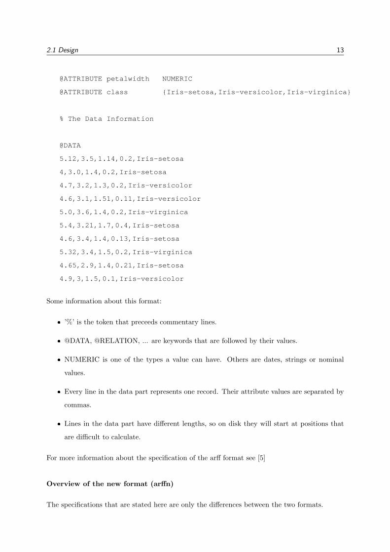
Some information about this format:
� ’%’ is the token that preceeds commentary lines.
� @DATA, @RELATION, ... are keywords that are followed by their values.
� NUMERIC is one of the types a value can have. Others are dates, strings or nominal
values.
� Every line in the data part represents one record. Their attribute values are separated by
commas.
� Lines in the data part have different lengths, so on disk they will start at positions that
are difficult to calculate.
For more information about the specification of the arff format see [5]
Overview of the new format (arffn)
The specifications that are stated here are only the differences between the two formats.

2.1 Design 14
ARFFN files have two distinct sections. The first section is the Header information, which is
followed by the Data information. The Header information is in standard readable text format,
but the Data information is in binary format, so not readable nor editable.
An example of the standard IRIS dataset would look like this:
@ARFFN
% 1. Title: Iris Plants Database
%
% 2. Sources:
% (a) Creator: R.A. Fisher
% (b) Donor: Michael Marshall (MARSHALL%[email protected])
% (c) Date: July, 1988
%
% The Header Information:
%
@RELATION iris
@ATTRIBUTE sepallength NUMERIC
@SIZE 8
@ATTRIBUTE sepalwidth NUMERIC
@SIZE 8
@ATTRIBUTE petallength NUMERIC
@SIZE 8
@ATTRIBUTE petalwidth NUMERIC
@SIZE 8
@ATTRIBUTE class {Iris-setosa,Iris-versicolor,Iris-virginica}
@SIZE 4
% The Data Information
@DATA ????
Changes:

2.1 Design 15
� The fist line (exactly the first!) should contain the ’@arffn’ keyword, specifying that this
file is a arffn file.
� After every attribute specification, there has to be a size specification (with the @size
keyword), which contains the exact size of the attribute value on disk (in bytes).
� The data part starts with the old @data-keyword, but is directly (not on a new line)
followed by the data information (in binary format).
There are two important remarks that can be made concerning this new format:
The @size-keyword specifies a fixed size of an attribute. Also of string attributes and this might
give some implications. Most likely strings have different lengths, so a maximum length should
be chosen. If a string is shorter it should be filled with ’dummy’ values (null characters).
This design choice has the disadvantage that datasets with some long strings may increase in
size unnecessary. But in actual Data Mining tasks, string attributes are rarely relevant and very
often the only string attributes appearing in datasets are short ones, such as record identifiers.
The binary representation is completely defined by the Java Specification and shouldn’t be
altered in any way. In the conversion between arff and arffn, the values will be written in the
default, standard way specified in the Java Specification. Neither the class designers nor the
Kiwi end users will be aware of how values are represented on disk. For example the conversion
of the dataset mentioned above, will write a sequence of 4 double values and 1 integer value to
the file, for every record in the dataset. The amount of bytes, little or big endian, etc. will all be
dependent on the Java Specification. A binary representation of numerical values has the benefit
that it might be less space consuming then a textual representation. This neutralizes more or less
the disadvantage of filling strings with dummy values, as is mentioned in the previous paragraph.
For more information about Java I/O: see [6] (Dutch) and [7] (English).
The conversion algorithm
Figure 2.1 shows the typical usage of the conversion algorithm (which is located in the Convert
class). When an Instances object is created, the arff file will be converted to an arffn file and
that file will then be forwarded to the DataSet class.
Basically what the algorithm has to do is the following:

2.1 Design 16
Figure 2.1: Sequence diagram explaining how an Instances object is created
� Read the header information from the arff file.
� Calculate the length of each attribute.
� Write the header information in arffn format to the target file.
� Write the data information in arffn format (binary) to the target file.
All these steps are quite straightforward, except for the second one: calculating the length of
each attribute. Difficulties arise when a string attribute is found. To be able to calculate the
maximum length for the string attribute, an iteration through the complete dataset is necessary.

2.1 Design 17
2.1.2 The Core classes
In order to alter Weka to be able to handle large datasets, some of its core classes need to be
changed. In particular the Instances class which represents a dataset. This class is one of the
most important ones, because it contains all the information about a dataset. The two main
features it has are:
� A vector that contains the attribute information of the dataset
� A vector that contains all the records of the dataset
In the further design of Kiwi the assumption is made that this first vector can remain in memory.
This will be true for almost all datasets, because it is rather rare for a dataset to have a few
millions of attributes. The second vector however is the one that needs to be changed. It should
be changed with a structure that allows all the records to remain on disk and loaded to memory
whenever this is requested. This structure will be a file on disk, so retrieving a record from the
dataset will result in a disk access. The design of this change has to be as clear as possible in
order to do complex optimizations without sacrificing the readability of the code. Considering
these requirements, the following options are possible:
� Keeping everything in the Instances object and make all the changes in that class.
� Keeping the attribute vector in the Instances object, but making a new class which
handles operations on the dataset.
� Making a new class that handles operations on the dataset and including the attribute
vector in that class.
The first approach is clearly the most unfavorable one, however the reason for this is not per-
formance, but code complexity. The Instances class already is very complex (>2000 lines), so
adding the very complex task of keeping the dataset on disk to that class is really too much.
The third approach seems very clean and transparent: the Instances class would redirect all
requests to that new class, without altering them too much.
But in the end the second approach seems the best because of the following two reasons:
The first is simplicity : all the necessary operations on attributes were already implemented in
the Instances class. Attributes don’t have to be put on disk, so their manipulation can stay

2.1 Design 18
in the Instances class.
The second is clarity : by putting the code for the manipulation of attributes in the Instances
class, we can keep the DataSet class a lot clearer. Instances handles the attributes, DataSet
the records.
Figure 2.2 shows the separation of the Instances class. Instead of a dictionary containing all
the Instances 1, just one single object is used in Kiwi: a DataSet. (See the Weka API [8] for
more information about the Weka class structure) This object will act as an intermediate layer
between the Instances object and the dataset on disk.
(a) (b)
Figure 2.2: (a) Part of Weka’s class diagram, (b) Part of Kiwi’s class diagram.
By doing it this way, all public methods of the Instances class will stay the same and for the
class user this change will remain invisible.
1It’s important to note that Weka uses Instance objects and Instances objects. This can be confusing.
To make things clear, most of the times the term ’record’ is used for an Instance. Sometimes however, if we
talk about the real class that is implemented in Weka (like now), the term Instance is used.

2.1 Design 19
2.1.3 The DataSet class
Introduction
In this section the design of the DataSet class is given. First the basic functionality is explained
and later on all optimizations such as prefetching, buffering, etc. are discussed. The pros
and cons of each optimization are carefully weighed against each other in order to reduce the
complexity, without sacrificing too much efficiency.
Basic functionality of the DataSet class
The basic functionalities the DataSet should have are:
� Retrieving of a random Instance (record) from the dataset.
� Adding an Instance to the end of the dataset.
� Removing a random Instance from the dataset.
� Removing an Attribute (column) from the dataset.
� Inserting an Attribute at an arbitrary location in the dataset.
Note that there is no insert operation for records. They can only be added to the end of the
dataset. This is an important advantage for the design.
In Weka all those functionalities were implemented by the Instances class. This class will act
as a transparent layer to the dataset on disk and will redirect all the requests to the DataSet
class. This class will then do the specific operation and will return the result to the Instances
class, which eventually passes the desired result on to whoever requested it. The sequence
diagram of one of those operations, namely the retrieval of an Instance, is given in figure 2.3.
The sequence diagrams of all other operations are quite similar.
The retrieve and add operation can be implemented quite efficiently (and straightforward). But
the other operations present some problems. In Weka, the records are saved in a vector. If a
record is deleted, all the records after that are shifted in the vector, which implies changing
their indexes. If the same thing is to be done on disk, that operation can be extremely slow. In
the worst case the entire dataset will have to be rewritten. Some proper enhancements will be
needed to make these operations feasible.

2.1 Design 20
Figure 2.3: Sequence diagram explaining how to get an Instance from the dataset.
These enhancements are discussed in the next few sections.
Materializing vs. Calculating
’Materialization’ is a term used for the immediate execution of a process, without thinking of the
possible consequences. A delete operation of one record would result, as is explained previously,
in rewriting almost the entire dataset.
’Calculation’ on the other hand, means that we would ’remember’ which record was deleted,
without actually removing it from the dataset on disk. In Kiwi, the latter option is used for
some of the basic functionalities mentioned above. It is used for removing records and attributes.
However it is not used for inserting attributes, for a reason which is explained later.
Note: It could also be used to insert records into the dataset at an arbitrary location, but this
functionality didn’t exist in Weka, so it isn’t introduced here.
For each of those 2 operations a table is kept with the indexes of the removed records or
attributes. Once the maximum size of those tables is reached, they will be materialized on disk.
This means rewriting the complete dataset, but without the deleted records or attributes. But,
for retrieving records (or deleting others), the exact location on disk should be calculated using
those ’remove’ tables. This increases the code complexity a little, but is justified by the increase
in performance. See figure 2.4 for the sequence diagram of the operation that deletes a record

2.1 Design 21
and figure 2.5 for an example of a remove table.
Figure 2.4: Sequence diagram explaining how to remove an Instance from the dataset.
Note that the remove table contains the indexes of the records on disk, not the indexes that the
user requested to be deleted.
If the user has deleted the first record (number 9, as can be seen in the ’User delete sequence’)
and then requests to remove record 11. The actual record that will be marked for deletion will
be number 12. Logically this is number 11, but physically on disk, this is still number 12.
Buffers
A second optimization that is included in Kiwi is the use of buffers. If the way Weka handles
datasets is examined in detail, one would notice that a lot of algorithms build up new datasets
starting from an empty one and performing add operations, without deleting any records until
the dataset is complete. This is the case, for example, when copying a dataset, a very frequent
operation in Weka. This has been one of the reasons why an add-buffer has been introduced to
Kiwi. The records that are consequently added to the dataset will be stored temporarily in a
add-buffer (or record-buffer). If that buffer is full it will be written to the dataset. By doing
this the amount of disk accesses are limited, which results in a big increase in speed.

2.1 Design 22
0123456789101112131415
3569
1215
ABCDEFGHIJKLMNOP
index record-value Removed indexes (ordered)
User delete sequence: 9 11 5 3 11 4
Records on disk: Remove table:
Figure 2.5: Example of a remove table
When another operation is requested, it will also result in a materialization of the buffer. The
buffer is always written to disk right before the execution of another operation. It is most unlikely
that add-operations are mixed with others, so keeping the add-buffer as it is (in memory), isn’t
really necessary and would only increase the complexity a lot.
See figure 2.6 for the sequence diagram of the add operation.
Additionally the inserting of attributes (the columns of the dataset) could be done with a
buffer. This isn’t done in Kiwi, again: to reduce the complexity, but also (and mainly) because
algorithms that add an attribute are quite rare. In those few cases where it does happen,
maximum one attribute is added, for example to include a summary attribute that summarizes
a record. Immediately after that operation all the values of the new attribute will be added, so
if a buffer was used, this would have meant materializing it directly after its creation.
Instead of including a buffer, the operation to add an attribute will be done immediately, which
implies that the complete dataset needs to be rewritten (because the length of a record has
changed).

2.1 Design 23
Figure 2.6: Sequence diagram explaining how to add an Instance to the dataset.
Prefetching
Prefetching is the act of retrieving records before they are requested. This approach is based
on caching, but is simplified a lot. Instead of using multiple pages, just one page is used. (see
[9], section 2.2.5 for information about caching). Caching techniques are based on two common
phenomena: spatial locality of reference and temporal locality of reference.
Spatial locality of reference observes that a resource is more likely to be referenced if it is near
another resource that was recently referenced.
Temporal locality of reference says a resource is more likely to be accessed if it was recently
accessed.
Data Mining algorithms in general have an enormous spatial locality (almost all records will
be read in a sequential way), but have no temporal locality at all (records that have been read
won’t be read again in the near future). Because of that, we can simplify the caching system a
lot. Multiple pages are useless, because we don’t need to keep records that we read in the past.
So, in the end a 1 page caching mechanism is used, or 1 prefetch buffer as it is called here. If a
record is to be retrieved the prefetch buffer is examined. If the record isn’t located in the buffer,
the buffer will be refilled with sequential records, starting from the record that was requested.
By prefetching records, we will limit the disk accesses a lot. Considering the very high cost of
disk access, this optimization will proof to be very useful.

2.1 Design 24
But there is one problem with prefetching. What if an algorithm retrieves instances in a non-
sequential way? Then every time a record is retrieved, the prefetch buffer will be refilled with
new records. So, instead of consequently reading records, Kiwi would consequently read groups
of records. This will reduce the efficiency a lot for non-sequential algorithms. An easy solution
is to let the algorithm decide if it wants to prefetch the next records or not. However this has
an important drawback, which will be discussed (together with a solution) in the next section.
As the default option, prefetching is set, because it is most likely that an algorithm will need it.
See figure 2.7 for the sequence diagram of the retrieve (or ’get’) operation.
Figure 2.7: Sequence diagram explaining how to retrieve an Instance with prefetching
Prefetch prediction
As mentioned in the previous section, prefetching has an important disadvantage. If records are
read in a non-sequential way and the algorithm has used the standard option for prefetching
(which is: prefetching enabled), then this will be very inefficient. But what can be done against
this misuse of prefetching? The answer is to dynamically predict whether prefetching is required
or not. This prediction should decide whether to refill the buffer if a record is requested that

2.1 Design 25
isn’t located in the buffer yet, or not.
If this problem is examined in more detail, again the analogy with a computer architecture
technique can be made. This time with a 2-bit instruction branch predictor. This predictor
will base its prediction on the two previous times the branch-conditions were evaluated. If the
branch was taken those two times, it will be predicted to take it again. If it wasn’t taken the
last two times, it won’t be taken again. To make the predictor more accurate, wrong predictions
will only be taken into account if they occurred more than 1 time.
To use this technique in Kiwi, almost the exact same thing will be done. There is just one
difference: with a branch predictor, the location where to jump to is known in both cases
(taking the branch, or not taking it). But with prefetching we can’t predict which record has to
be read if it isn’t the next. We can only predict that it’s not possible to use prefetching in that
case. So, the prediction will give an answer to the question: ”Is prefetching useful or not?” If the
answer is yes, the prefetch buffer will be refilled if necessary, if the answer is no, the requested
record will be retrieved from the dataset on disk directly, without any buffering.
A 2-bit dynamical prefetch predictor will be updated every time a decision has to be taken. It’s
functionality is described in figure 2.8. See [9], section 4.5.2 for more information about branch
predictors.
11 10
01 00
Prefetched
Not Prefetched
Predict to prefetch
Predict not to prefetch
Figure 2.8: Functionality of a 2-bit dynamical prefetch predictor

2.1 Design 26
Small improvements
Of course a lot of less important improvements are also possible. Whether they are useful or not,
largely depends on their theoretical frequency of occurrence in Weka. Most of these possible
improvements came to the surface while implementing the sample algorithms in the second
part of this thesis. By studying the way Weka launches and handles algorithms, some request
patterns to the dataset become clear.
In the remainder of this section, those small improvements that were implemented in Kiwi will
be discussed.
Empty prototype datasets are often used in algorithms. These are datasets without any records
in them, that are just used for a representation of the structure of a dataset. The attributes
are saved, together with some other information, but no records are kept at all. Of course
creating a file on disk (even if it just contains the header information and no records) is time
consuming. That’s why a file should only be created if instances are added to it. All the
necessary information is kept in memory.
Add-deleteLast sequences are used quite frequently while filtering a dataset in Weka. A filter
algorithm will read instances sequentially and will put each filtered one in a FIFO-queue. But
most of the time that queue does not consist of more then one instance. The pushed instance is
popped immediately. A FIFO queue is often implemented using an Instances object. Adding
a record, writing it to disk and immediately afterwards removing it again isn’t very efficient.
That’s why the record shouldn’t be written to file, but instead be kept in the add buffer and be
removed from that buffer directly. This way a time consuming disk access is avoided.
Small datasets should be kept in memory all the time, without doing any disk accesses. Small
datasets occur in numerous occasions: sometimes Weka is used to analyze a small dataset,
sometimes large datasets are being evaluated but the evaluation algorithm makes some small
datasets (for example datasets containing one cluster during a clustering operation), etc. To
keep those datasets in memory, it is possible to use the add buffer more extensively. Until that
buffer is exhausted we can keep all the records in it. Once it’s limit is exceeded the buffer has
to be materialized (written to disk). Again, this optimization will limit disk accesses a lot.
Buffer sizes. One remark has to be made about the size of the prefetch buffer and the add
buffer. This size might affect the final performance results a lot. There are two requirements
for the size:

2.1 Design 27
� They shouldn’t be ’too small’. At least a few times the disk-block-size.
� They should be a multiple of that block-size.
If they would be made too small, it would be a lot less efficient, because writing complete blocks
to disk is a lot more efficient than writing just parts. A block-size is typically 4 KiB (but
might vary from configuration to configuration). The higher that ’multiple’ of the block-size
the better, because that way the amount of complete blocks that will be written to disk will
be bigger. However making it too big will increase the memory usage and is therefore also
unfavorable. While doing some basic tests, the above remarks were proven to be correct and a
buffer size of 256 KiB was proposed.

2.1 Design 28
2.1.4 Adaptation of the other classes
As mentioned in 2.1.2 all these changes have to be made as transparent as possible to the other
(non-core) classes and packages in Weka. However, doing this in a complete transparent way
is not possible. The algorithms and the GUI have been programmed with the knowledge that
the datasets fit in memory and they use that knowledge occasionally. So, in order to function
correctly, Weka will need more adaptations then previously thought of. What follows are the
main changes that were needed.
Dataset history
A dataset history (or better known as the possibility to do an ’undo’ operation) is kept for
every dataset in Weka. Each time an algorithm is executed on the dataset, an entry in the
’history table’ is made. That entry consist of a copy of the complete dataset, which is of course
impossible in Kiwi, because datasets probably don’t fit in memory.
There are two solutions to this problem. One is to copy the entire dataset (on disk) to another
file and use the filename as the entry in that history table. But this has 2 major disadvantages:
it would be very slow, because we have to copy the entire dataset every time we execute an
algorithm, and it would be very space-consuming for secondary storage. A second option is
to not save the dataset history, but only the first original dataset file. If an undo-operation is
requested, the original dataset will be reloaded. With this solution all the problems are solved:
the history table would only contain the filename of the dataset, the dataset does not need to
be duplicated so no time is wasted and the dataset is not copied every time again, so we don’t
waste space on secondary storage. Of course the undo operation becomes quite basic with this,
but the disadvantages of having a full-operable undo option are far too big to make it justifiable.
Queues
Queues are, as mentioned in 2.1.3, often used while preprocessing datasets. A filtered record is
put on a FIFO-queue and can be retrieved a lot later. In Weka those queues are represented
by a kind of linked list of records that remains completely in memory. But sometimes all the
processed records from the dataset are pushed one by one, before a pop operation occurs. This
means that the entire dataset will be stored in that linked list in memory, which is of course
impossible.

2.1 Design 29
Again there are two possible solutions: one, alter the linked list so that it keeps its nodes on
disk instead of memory; another, to use a disk-based Instances object instead of a list. Since
the second data structure is already implemented, it was the obvious choice. A queue will then
be represented by an Instances object, the push operation is equal to an add operation and a
pop operation is equal to a deleteLast operation.
The queue belongs to an abstract class that is used as a prototype for every preprocess algorithm.
This class has some standard operations that have to be implemented in every subclass and has
some other operations (and variables) that are equal for every subclass (for example the queue).
This demonstrates the clever object oriented design of Weka and has facilitated the adaptation
of the preprocess algorithms to allow them to work with a queue on disk instead of memory. In
chapter 3 these object oriented techniques are discussed in more detail, because they are also
used for Clustering, Classifying, etc.
Visualization
The Visualization of a dataset results in some serious problems if large datasets are to be treated.
If a dataset is loaded in Weka, it will be read entirely to determine some basic statistics about it
such as the mean value, the standard deviation and the minimum and maximum values of each
attribute. A graph will be constructed that shows the values of a particular attribute. For this
graph an array is constructed containing all the values of that attribute.
These properties have as a consequence that the visualization of the dataset will be very slow
(iterating the entire dataset) and might even be impossible. It will be impossible if an array
containing all the values of one attribute is too big to be kept in memory. A logical solution
is to limit the amount of records that are visualized. For visualizing the values it really isn’t
necessary to get the information of every possible record. Visualizing millions of records is
useless, because neither the computer screen nor the human eye or mind can handle this much
information. That’s why in Kiwi only a random sample (500 records) of the dataset will be used
for visualization.

2.2 Implementation 30
2.2 Implementation
Introduction
In this part the implementation of Kiwi is going to be discussed. The implementation will follow
the design that was proposed in the previous part. The specialized techniques that are used
are discussed in depth, focusing mainly on the efficiency. However this part will not go into too
much code details, because they are of minor importance to the final result. For more detailed
information about the implementation, see the generated API information or the code itself,
which are both located on the CD-ROM that is included with this thesis.
2.2.1 Java.nio
One of the disadvantages of Java is that its IO performance is inferior to that of other pro-
gramming languages. At least, that was a disadvantage in the past. Since Java 1.4 this has
changed with the introduction of the New I/O API (NIO). NIO concentrates on providing con-
sistent, portable APIs to access all sorts of I/O services with minimum overhead and maximum
efficiency. NIO eliminates many of those performance issues, allowing Java to compete on an
equal footing with natively compiled languages. It includes many critical things to write high-
performance, large-scale applications. The buffer management, scalable network and file I/O all
have improved a lot. That is why this new API is used as much as possible in this thesis. In
Kiwi a lot of data is transfered or copied from disk to disk, from memory to disk or from disk
to memory and of course it is this I/O that produces the main bottleneck. More information
about the Java.nio package can be found on [10] (Dutch) and [11] (English).
One thing that is particularly fast in NIO is writing huge amounts of sequentially located data
from one place on disk to another. This is done with two basic structures of NIO: Buffers and
Channels. A typical sequence would be something like this: (details are omitted)
FileChannel chanIn = new FileInputStream(...).getChannel();
FileChannel chanOut = new FileOutputStream (...).getChannel();
ByteBuffer buf = ByteBuffer.allocateDirect(4 * 1024);
while (chanIn.read(buf) != -1){
manipulate(buf);
chanOut.write(buf);

2.2 Implementation 31
}
chanIn.close();
chanOut.close();
This example uses a buffer of 4 KiB to read data from a file, manipulate it and write it to
another file. Because NIO is used, this will be faster then with the classical I/O API.
Sequences like the above one will be frequently used in Kiwi. They will be used for the following
operations:
� Conversion between arff and arffn format: the entire dataset needs to be read, manipulated
and written to another file.
� Materialization of the add buffer: every time this buffer is full, it will be written to the
dataset
� To make an exact copy of the dataset: used for saving a dataset for future usage.
2.2.2 MappedByteBuffer vs RandomAccessFile
However to access a particular record (or a number of sequential records), the above method
can’t be used. A random access to the file is necessary. This is supported in the classical I/O API
by a RandomAccessFile. The equivalent in NIO is a MappedByteBuffer. Both structures are a
mapping to the file on disk. A file pointer exists which can be positioned on an arbitrary location
on the file. A read operation will then get an amount of bytes from that location. However
a MappedByteBuffer will do this more efficient and will take virtual memory techniques into
account.
There is one small particularity that makes this MappedByteBuffer useless however. This par-
ticularity is stated in the Java API (see [12]):
”Many of the details of memory-mapped files are inherently dependent upon the underlying op-
erating system and are therefore unspecified. Whether changes made to the content or size of
the underlying file, by this program or another, are propagated to the buffer is unspecified.”
This makes it impossible (for example) to know what would happen if we try to enlarge the
buffer. This operation is necessary in Kiwi if we want to add records to the end of the dataset.
So, enlarging the file is impossible (sometimes it would succeed, sometimes not). Another pos-
sibility is to close the file, enlarging it, and reopen it afterwards. However this isn’t possible
2.2 Implementation 32
because a MappedByteBuffer is automatically closed when it is garbage collected. It does not
have its own close operation. Closing the underlying RandomAccessFile isn’t allowed either.
All together the use of a MappedByteBuffer is not possible, so the classical Java I/O API will
be used for ’position-based’ retrieval of records. With position-based retrieval is meant the
retrieval of records starting at a random position in the dataset. The operations mentioned
in the Java.nio section read the complete dataset (or read a complete buffer), but don’t need
positioning in it.
A RandomAccessFile will be used for the following operations:
� Filling the prefetch buffer: starting at the position of the requested record, until the buffer
is full (or the end of the dataset is reached).
� Retrieving a record without prefetching.
� Inserting an attribute: positioning is necessary if the dataset is not to be copied but
overwritten (more information in section 2.2.4).
� Swapping of two random records.
� Materialization of the remove tables: if copying of the dataset is to be avoided (overwriting
the dataset is wanted instead), positioning will be necessary (more information on section
2.2.4).
2.2.3 ByteBuffer vs Byte array
For the prefetch buffer and the add buffer some kind of data structure is necessary that holds
records in binary format. Again there is a solution with the NIO API (a ByteBuffer), which can
be compared to a more usual structure. (a simple Byte array). Both solutions can be used in
the same way, so the first implementation of Kiwi contained a ByteBuffer (because of the better
performance of NIO). But after testing, a major drawback was encountered.
ByteBuffers are a lot more memory consuming then simple Byte arrays. Most likely they are
garbage collected a lot later then Byte arrays. In a preliminary version of Kiwi a ByteBuffer
was created, used and overwritten with another one, quite frequently. With this sequence the
memory usage kept increasing. By replacing the ByteBuffer with a Byte array and keeping
the exact same sequence, the memory usage did not increase at all. That’s why in the current
version of Kiwi ByteBuffers aren’t used as a prefetch buffer or an add buffer.

2.2 Implementation 33
2.2.4 Materialization
Recall that there are three operations on datasets that, if done naively, imply rewriting the entire
dataset: deleting records, deleting attributes, and inserting attributes. The first two of those
operations will be ’saved’ temporarily and materialized when necessary to limit the amount of
disk accesses. The third one however will be executed immediately on disk.
The desired way to perform those operations is by overwriting the original dataset and not
duplicating it. Of course records can only be overwritten if they won’t be needed afterwards.
NIO facilitates this process remarkably: a buffer of data is loaded, a transformation is made to
it and then it is written to the appropriate position (see the pseudo code in section 2.2.1).
For the first two operations (deleting records and attributes), this can be done quite straight-
forward: (details are omitted)
int readPosition = 0;
int writePosition = 0;
while (readPosition < dataset.length())
{
file.read (buffer, readPosition);
readPosition += buffer.length();
discardDeletedRecords(buffer);
discardDeletedAttributes(buffer);
write(buffer, writePosition);
writePosition += buffer.length();
}
This can be done with the knowledge that the buffer will not be expanded before writing it
to the dataset. If it would have expanded, some records that have not yet been read could be
overwritten.
However this will not work for the last operation (inserting an attribute), because here the buffer
will expand. One solution would be to write the dataset to a new file, but this is of course a
useless waste of resources. Another solution, and that is the one that is used in Kiwi, is to
rewrite the dataset backwards. The final size of the dataset can be predicted (because the new
attribute has a fixed size), so the updated dataset can be written backwards starting at the end
of the file.

2.2 Implementation 34
In pseudo code (without details) it could be stated as follows:
int readPosition = (numberOfRecords * oldRecordSize)
- oldBufferLength;
int writePosition = (numberOfRecords * (oldRecordSize + attributeSize))
- newBufferLength;
while (readPosition >= 0)
{
file.read (buffer, readPosition);
readPosition -= oldBufferLength;
addNewAttribute(buffer);
write(buffer, writePosition);
writePosition -= newBufferLength;
}
2.2.5 Object Finalization
In order not to waste any valuable resources, the temporary files that are created to store a
dataset need to be ”garbage collected” also. Garbage collection is a java technique in which
the memory resources will be released after an object goes out of scope. This won’t be done
immediately, but ”somewhere in the near future” (when exactly is implementation dependent
of the virtual machine). However, not only the memory resources need to be released, but also
the disk resources. This can be done with a Java feature called Object Finalization, which is
explained in detail in [13].
Basically, what has to be done is redefining an inherited operation from the Object class:
protected void finalize() throws Throwable {
file.delete();
super.finalize();
}
This will have as a consequence that the temporary file will be deleted once the dataset goes
out of scope.

2.2 Implementation 35
2.2.6 Conclusions
Although for some purposes the Java.nio API is a big improvement on the classical I/O in Java,
it has some serious disadvantages concerning memory management and flexibility. But, it isn’t
a substitute for that classical I/O API, it’s more of an addition to it. Some of the problems
mentioned here will probably be solved in future Java releases, but for now a combination of
the two different API’s seemed a good solution and proved to be quite efficient (as will be seen
in the next section).

2.3 Performance 36
2.3 Performance
2.3.1 Introduction
The following performance tests were run on an AMD 1800 Ghz, with 512 MiB RAM and Win-
dows 2k running. The test datasets are sets with records that consist of 2 numerical attributes,
which means that each record will be 16 bytes long in arffn format. Having 2 attributes of 8
bytes or 1 of 16 or something else, doesn’t really matter, because to read a record a byte-stream
of 16 bytes will be read. Splitting this stream to the different attributes is done in main memory
which won’t affect performance.
The results are given in milliseconds (ms).
Tests are run with datasets of different sizes, ranging from 160 KB (10.000 instances) to 40 MB
(2.500.000 instances)
Five different tests are performed: (x is the amount of instances that are handled, or the amount
of times a particular sequence is performed.
� Loading a dataset of x records into Weka/Kiwi
� Sequentially reading all records of a dataset containing x records
� Non-sequential reading all records of a dataset containing x records (between record n and
n+1 there will be at least x/2 records.)
� Adding x records to a new dataset
� Doing an add-deleteLast sequence x times
These tests represent the most common tasks in Weka/Kiwi and were also the basis of the design
of Kiwi. Some types of tests are missing (for example inserting an attribute, deleting random
records, ...), but they really aren’t that important for the overall performance.
The tests are done directly on the Instances class, without loading the GUI etc. This means
that a better performance will be measured for Weka then what is actually the case. This has
been done to keep the results clear enough for evaluation. The time for loading a dataset for
example, really is the time for loading the dataset. No other interfering operations are performed
(such as determining some statistical values, visualizing the attributes, etc.).
2.3 Performance 37
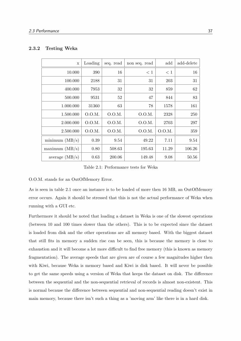
2.3.2 Testing Weka
x Loading seq. read non seq. read add add-delete
10.000 390 16 < 1 < 1 16
100.000 2188 31 31 203 31
400.000 7953 32 32 859 62
500.000 9531 52 47 844 83
1.000.000 31360 63 78 1578 161
1.500.000 O.O.M. O.O.M. O.O.M. 2328 250
2.000.000 O.O.M. O.O.M. O.O.M. 2703 297
2.500.000 O.O.M. O.O.M. O.O.M. O.O.M. 359
minimum (MB/s) 0.39 9.54 49.22 7.11 9.54
maximum (MB/s) 0.80 508.63 195.63 11.29 106.26
average (MB/s) 0.63 200.06 149.48 9.08 50.56
Table 2.1: Performance tests for Weka
O.O.M. stands for an OutOfMemory Error.
As is seen in table 2.1 once an instance is to be loaded of more then 16 MB, an OutOfMemory
error occurs. Again it should be stressed that this is not the actual performance of Weka when
running with a GUI etc.
Furthermore it should be noted that loading a dataset in Weka is one of the slowest operations
(between 10 and 100 times slower than the others). This is to be expected since the dataset
is loaded from disk and the other operations are all memory based. With the biggest dataset
that still fits in memory a sudden rise can be seen, this is because the memory is close to
exhaustion and it will become a lot more difficult to find free memory (this is known as memory
fragmentation). The average speeds that are given are of course a few magnitudes higher then
with Kiwi, because Weka is memory based and Kiwi is disk based. It will never be possible
to get the same speeds using a version of Weka that keeps the dataset on disk. The difference
between the sequential and the non-sequential retrieval of records is almost non-existent. This
is normal because the difference between sequential and non-sequential reading doesn’t exist in
main memory, because there isn’t such a thing as a ’moving arm’ like there is in a hard disk.

2.3 Performance 38
2.3.3 Testing Kiwi
x Loading seq. read non seq. read add add-delete
10.000 359 32 2141 47 78
100.000 1797 140 21250 171 125
400.000 6969 563 84578 968 515
500.000 8484 640 106125 1375 610
1.000.000 17531 1281 211469 2453 1250
1.500.000 27641 2000 336953 3203 1844
2.000.000 36047 2688 447312 5234 2468
2.500.000 49875 3250 564781 6078 3078
minimum (MB/s) 0.43 4.77 0.07 3.25 1.96
maximum (MB/s) 0.90 11.92 0.07 8.92 12.51
average (MB/s) 0.79 10.61 0.07 6.19 10.99
Table 2.2: Performance tests for Kiwi
The first and most important conclusion that can be taken is that Kiwi keeps working, even
for large datasets. But also the performance is quite good. Loading the dataset (including a
conversion to arffn which implies that the dataset is rewritten) is as fast as with Weka. The
main reason for this is the use of Java.nio, which makes reading data from disk faster than
with the classical I/O API. The sequential retrieval and the add operation have remarkable
performances: 10 MB/s, resp. 6 MB/s, on average. This is close to the maximum that could
have been expected. This, in comparison with non-sequential retrieval, proves the correct and
efficient use of the prefetching and buffering. Also in Kiwi the difference of performance for the
sequential retrieval compared to the non-sequential one is quite high. In Weka however these
operations have the same performance. This can be explained by noting that main memory has
no seek-delay, while that delay is quite big when secondary storage is used.
Of course these values are influenced by a lot of things:
� The fragmentation of the hard disk: running these tests on a very fragmented or on a
recently de-fragmented disk might give very different results.
� Amount of space left on the hard disk: when a large dataset is put on disk, it will hardly
ever be put in sequential blocks. The more space is available, the more likely it is that the
2.3 Performance 39
blocks will be closer together.
� Memory fragmentation: if the available memory becomes limited it will be slower to put
something on memory (because an empty block has to be found).
� The disk usage on the time of the performance tests: some swapping might occur, some
other programs might be running in the background, etc.
As a final conclusion of the performance the following points can be noted:
� Kiwi works for all sizes of datasets, without limitations or OutOfMemory errors.
� Prefetching works, which can be seen with the performance of the sequential retrieving.
This operation is very fast compared to non sequential, and ’only’ 20 times slower than in
Weka.
� Add buffers work, which is noted in the performance of the add operation. This operation
is only two times slower than in Weka.
� Loading works very fast. This is due to the use of NIO, but also to the fact that the
records aren’t loaded at all. They stay on disk until they are retrieved.
� The only down side is the non-sequential retrieval of records. This is about 100 times
slower than the sequential retrieval. This result is however quite normal because it is
always the case with secondary storage. Luckily most Data Mining algorithms retrieve
records in a sequential way. This will prove to be a problem with the sampling algorithms
that are discussed next.

SAMPLING ALGORITHMS 40
Chapter 3
Sampling algorithms
3.1 Introduction
This chapter describes the second part of this thesis. It consists of the implementation of some
theoretical sampling algorithms. These algorithms are designed by the director of this thesis
(Gavalda Mestre, Ricard), who has written, together with others, some papers about random
sampling in Data Mining. For this thesis, two well-known data mining algorithms were chosen
and sampling versions of these were developed using the techniques in [4]. An implementation
will be given of a clusterer: Sample K-Means and a classifier: Sample Naıve Bayes.
Random Sampling algorithms in general are used as an alternative to the normal ’sequential’
Data Mining algorithms. They will look at some random records from a dataset until they decide
that enough records have been read to get to a final result. This final result will approximate
the ’correct’ result that would be obtained if a non-sampling algorithm was used. Sampling
algorithms are useful when datasets are too big to be used with non-sampling algorithms. These
algorithms slow down a lot if the datasets get bigger. Typical, they iterate through the entire
dataset a few times before delivering a result.
The two sampling algorithms will be based on their non-sampling counterparts, which both have
some existing implementations in Weka. These implementations will be used as a basis for the
new ones.
As a last point in this introduction it should be stated that these algorithms and their imple-
mentations are purely for scientific research. A theoretical design was made and together with
the implementation, some conclusions will be made on the performance, the correctness, etc.

3.2 Sample K-Means 41
The implementation will be based on that basic assumption, so further optimizations will be
discussed, but not implemented, in order to come to correct conclusions of the original proposed
theoretical algorithms.
3.2 Sample K-Means
3.2.1 Design
The algorithm
Sample K-Means is a sampling algorithm based on the well known K-Means clustering algorithm.
The goal of this algorithm is to find K clusters in a dataset. A cluster can be defined as a set
of points (or records) that have very close values. Finding clusters in a dataset can be a way
to retrieve some valuable information from a dataset. For example a clustering algorithm could
be executed on a dataset containing characteristics of stars: spectrum, color, distance, age,
brightness, etc. Clustering could be used to automatically find structural groups in them (blue
ones, red ones, novas, supernovas, quasars, giant and dwarfs of different types).
However a dataset like this could be updated constantly by gathering information from radio
telescopes that constantly scan the sky. Many new stars are found every day, so in the end the
dataset would become enormous. Clustering those records with a non-sample algorithm would
be very time consuming, because all records will be sequentially read, probably more than once.
This is one of the many examples where sequential clustering is not desirable. A sampling
clustering algorithm will incorporate a stopping condition that evaluates to true the moment
that the resulting clusters are ’likely’ (in a statistical way) to be the correct ones. The proposal
for the Sample K-Means clustering algorithm can be found in Appendix A.
For more information about the normal K-Means clustering algorithm, the book where Weka
was first introduced could be consulted [1]. This algorithm has been introduced several times,
by different independent persons, so J.H. Ward [14] and J.C. Gower [15] should be mentioned
also.

3.2 Sample K-Means 42
Clustering algorithms in Weka/Kiwi
Weka is programmed in Java, an object oriented programming language, which facilitates the
software design a lot. In Weka a lot of design techniques are used to obtain an easily readable
and maintainable program. It also offers a clear and transparent structure for future extension
and new algorithm implementations.
The structure of the clusterer package is given in figure 3.1, which shows the Sample K-
Means class that is to be implemented, together with an example of one of the other algorithms
in that package (Simple K-Means). To implement a new algorithm, the prototype clustering
class should be extended. This class (”Clusterer”) has some abstract operations that need to
be implemented. That way a totally transparent handling of new algorithms is possible. To
add a new clusterer algorithm, the implementation class (which extends the prototype) should
be put in that package and an entry should be made in the property file of Weka. This file
contains a list of all the different algorithms. Note also that an OptionHandler interface should
be implemented, if user input is required in the algorithm (the number of wanted clusters for
example).
Figure 3.1: Class diagram explaining the design structure for clusterers.
3.2.2 Implementation
The basis
In pseudo code the algorithm looks as follows: (for a more complete design see Appendix A)
take k random centroids (k = the number of desired clusters)

3.2 Sample K-Means 43
while (not stable){
while (stopping condition not true){
r = random record from dataset
j = closest cluster for r
accumulate r to the total sum of cluster j
if (smallness condition true){
mark small clusters
}
update statistics needed for the stopping condition
}
change centroids to the average of their cluster values
}
Basically the algorithm will retrieve random records from the dataset until the stopping condition
is true. This stopping condition is based on some statistics that are used to compute the
probability that with the records read so far, a good approximation already is found or not.
These statistical values will be updated at each iteration of the inner loop. Clusters will be
marked ’small’ only one time at each iteration of the outer loop, if the smallness condition
evaluates to true. This is the case if enough records have been read to be able to discard the
clusters that are too small to take into account. After that inner loop (if the stopping condition
became true), the centroids (average value of the clusters) will be updated with the average of
the points (or records) that have been assigned to it. This last step is the same as in the non
Sampling algorithm.
Both of the conditions (stopping and smallness) depend on some user input values. They are
defined as follows:
� ε: The margin that is allowed for a point to be put into the wrong cluster. If a point is a
fraction of ε (relative) away from the border of two clusters, it will be put into the correct
cluster. If it is ε (relative) close to the border of two clusters, it may be put in the wrong
one. (standard value is 0.5)
� θ: A cluster is θ-large if it contains a fraction ≥ θ/k of the total amount of records. Note
that in average a cluster contains a fraction of 1/k of points. Only clusters that are θ-large
are guaranteed to be well approximated by the algorithm. Clusters with fewer points are
3.2 Sample K-Means 44
too expensive to approximate well, so the algorithm will not spend extra time waiting for
these. These clusters will not be dropped, the algorithm will just not wait for them to be
very well approximated, as given by ε. (standard value is 0.5)
� δ: The failure probability. In all sampling algorithms, there is a chance that the randomly
chosen points are very a-typical (for example, that by pure chance no point is found from
a fairly large cluster). The claims that are made about ε and θ will occur with probability
at least 1− δ. (standard value is 0.1)
The details
To be able to give an implementation of a theoretical algorithm design, some topics will need to
be dealt with, that aren’t yet discussed in the design. Some of them, especially the statistical
problems, are solved in co-operation with the director of this thesis, who is responsible for the
theoretical design of the algorithm.
Calculating the maximum and minimum values is needed for some various tasks: for
choosing k random centroids, for evaluating the stopping condition and to perform a normaliza-
tion of the values. The problem is that it is not desirable to iterate through the entire dataset
to determine these values, because this is exactly what is tried to be avoided with sampling.
The maximum and minimum values should be determined with a statistically correct approxi-
mation. To determine such an approximation, the maximum and minimum value of a sample
of the entire dataset will be taken instead. The size of that sample will be computed with the
following formula:2d
δln
(2d
δ
)Where ’d’ is the number of attributes in the dataset.
This formula is correct for a fraction 1 − δ of the points. If δ = 1 at least 90% of the points
will have all their values between the maximum and minimum that is computed. The (at most)
10% remaining records may be discarded because some of their values are too ’strange’.
This step could be avoided if the maximum and minimum value of a dataset was known before-
hand. For example a Data Mining tool (such as Weka or Kiwi) could have retrieved some basic
statistics of a dataset when loading it.

3.2 Sample K-Means 45
Testing for empty clusters was missing in the original design, but is quite important. It
can occur that the stopping condition evaluates to true but that there is one cluster that does
not contain points. For this cluster the centroids can’t be updated (because there are no values
to calculate the average). But, if this centroid is kept, then in the next round again values will
be looked for that cluster. This will slow down the algorithm, because there are (most likely)
almost no points that belong to that centroid. That’s why this cluster will be ’dropped’. As
a consequence the final result will not contain the requested amount of clusters. However the
result will be delivered faster and without a big sacrifice. Very small clusters probably represent
erroneous values that can be discarded.
Nominal values. The algorithm has been designed to deal with numeric attributes only, not
nominal ones. The problem is the updating of the statistical values that are used for the stopping
condition. This stopping condition has to evaluate to true if enough points have been seen to be
sure of an approximately correct clustering. After this stopping condition the centroids will be
recalculated using the average of the values assigned to a particular cluster. However calculating
the average of nominal attributes might lead to erroneous results. What if the average is almost
in the middle of 2 nominal values? For example: if the average of a nominal value (which has
as possible values 0 and 1) is 0.499, then ’0’ would be taken as the average. Of course this isn’t
very meaningful.
Another reason for not including nominal values is that clustering is based on the notion of
”distance” between points. Distance among nominal attributes is a complicated notion.
Random generating of records is one of the topics that the algorithm leaves open for
discussion. The algorithm proposes a (theoretical) infinite array of records. This array will be
read more then 1 time, so the records (or their indexes) that are read will have to be stored. A
possibility for this is using a random generator with a fixed seed. If this generator is created a
second time (with the same seed), it will generate exactly the same sequence of numbers. Doing
it this way, the generated numbers can be used as the index in the dataset. This means we do
not have to store the records (or their indexes) that were read.
The seed will be a user input variable.

3.2 Sample K-Means 46
Other details are ignored here, because they don’t really have anything to do with the
’sampling’ part of this algorithm. For these problems the implementation of other algorithms,
that were already implemented in Weka, is used as a reference. For example the way values are
normalized, the way the distance between points is calculated, etc.
3.2.3 Performance
First test: Synthetic Control
In order to measure the correct performance of Sample K-Means a well known dataset is used:
The Synthetic Control Chart Series. This dataset contains 600 examples of control charts syn-
thetically generated by the process in Alcock and Manolopoulos (1999). It was taken from the
”UCI repository of machine learning databases” [16].
However, it’s extremely difficult to evaluate the accuracy of a clustering result. The only mean-
ingful measure would be to measure the intra and intercluster distances, but these are not
supported by Weka. Even with those methods different results can be labeled as correct. This
is because K-Means is an unsupervised learning algorithm. There is no way of knowing how
correct the result is.
K-Means is known to be unstable, because taking different random centroids in the beginning
of the algorithm, can lead to different clusterings. So even without sampling, it is difficult to
evaluate K-Means and the evaluation will only depend on the subjective interpretation that
somebody could give to the clusters, based upon his or her knowledge of the problem and its
domain. An explanation of this instability can be found at [17]. The best that can be done is
comparing the resulting centroids with the results obtained with a sequential algorithm.
With this Synthetic Control dataset the difference between the Sampling algorithm and a normal
K-Means algorithm will be evaluated. The most important measurement is the amount of records
that have to be read in order to come to a result.
Figure 3.2 shows the relationship between the two algorithms for different ε values. To repeat:
ε is the margin that is allowed for misclassified points.
It should be noted that the smaller ε becomes, the more records will be read using Sample K-
Means. But with a value of 0.5 (or even 0.3 for a small amount of clusters), Sample K-Means will
read a lot less records than K-Means. In table 3.1 the exact values are shown.

3.2 Sample K-Means 47
0,00
5000,00
10000,00
15000,00
20000,00
25000,00
30000,00
35000,00
40000,00
45000,00
0,5 0,3 0,1epsilon
#rec
ords
SampleKMeans (k=2)SampleKMeans (k=3)SampleKMeans (k=5)SimpleKMeans (k=2)SimpleKMeans (k=3)SimpleKMeans (k=5)
k=2k=3
k=5
Figure 3.2: Comparison chart between sampling and non-sampling K-Means with the Synthetic
Control dataset
With these exact values it should be noted that for ε = 0.5 and a small amount of clusters,
Sample K-Means will read a lot less records and produce more or less1 the same result. If the
dataset size would be a lot bigger (multiplied by 10 for example), this positive result could even
be expanded: The 3 horizontal lines representing the normal K-Means algorithm will be placed
10 times higher, but the graphs for the sampling algorithm would remain the same. This is
because the sampling algorithm reads as much data as necessary to reach a safe conclusion, but
not more.
Second test: an obvious dataset
To be able to decide a little more clear that the clustering really works, another dataset was
constructed. This dataset was deliberately made very obvious. Records containing two (nu-1Note that we use this subjective term, because (as explained before) comparing clustering results is rather
subjective.

3.2 Sample K-Means 48
#clusters ε #records with #records without
Sampling Sampling
2 0.1 2853 2400
0.3 252 2400
0.5 85 2400
3 0.1 11172 6000
0.3 409 6000
0.5 231 6000
5 0.1 42663 9600
0.3 13248 9600
0.5 3368 9600
Table 3.1: Comparison between sampling and non-sampling K-Means with the Synthetic Control
dataset
merical) values were used, in order to construct a dataset of four clear clusters, without overlap
between them. All the values are in the range [0,15] and the 4 centroids are: (2.5,2.5), (12.5,2.5),
(2.5,12.5) and (12.5,12.5). Values are randomly generated, but will always be close to one of
those four centroids. The dataset consists of 500000 records. To cluster the four clusters in it,
Simple K-Means will need to read 2000000 records (each record 4 times).
Another purpose of using this dataset, is to demonstrate the impact of the user input variables
(ε, δ and θ).
The results are given in figure 3.3 and in table 3.2.
Some notes and observations:
� When altering one user input value, the others are kept on their standard value (ε = 0.5,
δ = 0.1, θ = 0.5).
� These standard values seem to be quite good, because while using them, the amount of
records that will be read is limited and the results are (approximately) correct.
� With this dataset the correctness of the clusters can be easily seen by looking at the
values for the centroids. The centroids were always close to the centroids that were given
by Simple K-Means. Only for the highest values (close to 1) some errors occurred.
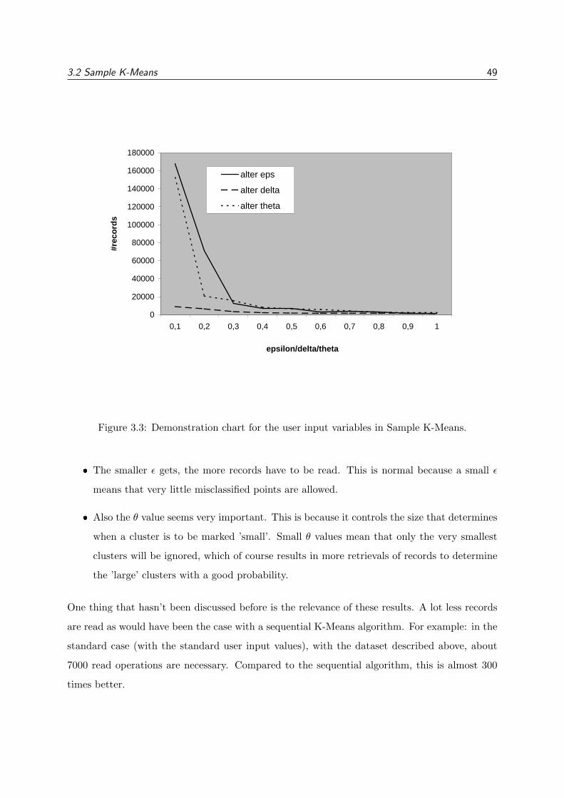
3.2 Sample K-Means 49
0
20000
40000
60000
80000
100000
120000
140000
160000
180000
0,1 0,2 0,3 0,4 0,5 0,6 0,7 0,8 0,9 1
epsilon/delta/theta
#rec
ords
alter eps
alter delta
alter theta
Figure 3.3: Demonstration chart for the user input variables in Sample K-Means.
� The smaller ε gets, the more records have to be read. This is normal because a small ε
means that very little misclassified points are allowed.
� Also the θ value seems very important. This is because it controls the size that determines
when a cluster is to be marked ’small’. Small θ values mean that only the very smallest
clusters will be ignored, which of course results in more retrievals of records to determine
the ’large’ clusters with a good probability.
One thing that hasn’t been discussed before is the relevance of these results. A lot less records
are read as would have been the case with a sequential K-Means algorithm. For example: in the
standard case (with the standard user input values), with the dataset described above, about
7000 read operations are necessary. Compared to the sequential algorithm, this is almost 300
times better.

3.2 Sample K-Means 50
ε/δ/θ values #records when altering ε #records when altering δ #records when altering θ
0.1 167953 8950 152402
0.2 70931 6516 20876
0.3 12351 3494 15645
0.4 7171 2262 8243
0.5 7085 1886 6540
0.6 3201 1617 5842
0.7 3553 1698 4232
0.8 3252 1785 2762
0.9 1451 1808 2392
1.0 1302 1184 2360
Table 3.2: Demonstration for the user input variables in Sample K-Means.
3.2.4 Weka vs Kiwi
If Kiwi is used with this algorithm instead of Weka, the above results should be rescaled. Sample
K-Means will retrieve the records in a non-sequential way. This kind of retrieval is a lot slower
than sequential retrieval in Kiwi. In Weka however, they are almost equal. This is one important
conclusion, because in principle a heavy price (concerning time complexity) is paid for using both
sampling and disk accesses at the same time. Sampling may seem redundant because of this,
but it isn’t. A sampling algorithm (or at least its ideas) could be used in a sequential way if
the data is received completely disordered. If this is the case, reading the next record is the
same as reading the next random record. The dataset will be read sequentially as in a normal
K-Means algorithm and with the same speed, but because sampling is used, it won’t be read
entirely.

3.3 Sample Naıve Bayes 51
3.3 Sample Naıve Bayes
3.3.1 Design
Classifiers in general
The goal of every classifier algorithm is to predict a nominal value, based on the values of the
attributes (except that nominal value) of a record. This can be used to make a guess for this
particular attribute when a new record is found, but with that data missing.
For example: classification could be useful to predict whether a new customer will refund a loan
that will be granted to him. Predicting that the loan will not be refunded, could be used as a
warning, but of course will not be 100% accurate. The prediction will be based on the other
attribute values of the customer: marital status, bank balance, previous loans, ... But also on
the data of the previous customers and whether they refunded the loan or not.
However, to give accurate results (or with an accurate representing error percentage), a big
dataset is preferred. This brings us back to the reason why sampling will be introduced. A
sequential classifier algorithm will typically read the entire dataset one time in a sequential way,
which might be very time consuming.
Sampling will limit that amount by incorporating a stopping condition which evaluates to true,
as soon as the resulting classification model is ’likely’ (in a statistical way) to be correct.
In this thesis Sample Naıve Bayes, which is based on Naıve Bayes, will be implemented.
Naıve Bayes
Naıve Bayes algorithms try to estimate the conditional probability of each class, given that the
record has some given values at the attributes. In symbols this is: Prob[class = c|attribute values].
By some derivation that is omitted, this probability can be estimated with the conditional prob-
abilities Prob [A = v|class = c] (for every individual attribute A and every one of their possible
values v). These probabilities, in turn, can be estimated also. For this estimation the following
two things are needed:
� The number of instances in the dataset having class c, which is denoted by classcount[c].
� The number of instances in the dataset having class c and value v in A, which is denoted
by count [c,a,v].

3.3 Sample Naıve Bayes 52
The main loop of the algorithm will iterate over the dataset in order to compute these classcount
and count values.
The idea of sampling, is to avoid running over the dataset if, from the instances seen so far,
good enough approximations to all the count and classcount values can be deduced. This
’good enough approximation’ will be controlled by a parameter (this will be ε1 in Sample Naıve
Bayes). If some of these values are too small, it will be difficult to approximate them correctly
with sampling. These values will be ignored so no valuable time is spent approximating them
further. To determine when a value is small a second parameter is introduced: ε2.
One could make the analogy with Sample K-Means of course. There ’clusters’ will be discarded
if they are too small, here those clusters will be the ’values’.
The proposal for the Sample Naıve Bayes algorithm can be found in Appendix B.
For more information about the normal Naıve Bayes algorithm the Weka book [1] can be con-
sulted. Again (as with K-Means) this algorithm has been ’rediscovered’ by several different
independent persons, of which [18] and [19] should be mentioned.
Classifier algorithms in Weka/Kiwi
Figure 3.4 explains the design structure for classifiers.
Figure 3.4: Class diagram explaining the design structure for classifiers.
This structure is almost identical to the structure for clustering. The same reasons and benefits
can be noted here. For more information see the description in the section about Sample K-
Means (3.2.1).

3.3 Sample Naıve Bayes 53
3.3.2 Implementation
The basis
In pseudo code the algorithm looks as follows: (for a more complete design see Appendix B)
/ * compute counts: * /
while (stopping condition not true){
r = random record from dataset
increment the counts and the classcounts
update statistical values used for the stopping condition
mark the class c, or the value c,a,v small if necessary
}
/ * compute prior class probabilities and conditional probabilities: * /
for (all classes c){
for (all nominal attributes a){
for (all values v of the attributes){
cond[c][a][v] = compute probability of the v to the class c
}
}
prior[c] = compute the prior class probability
}
Basically the algorithm will first retrieve random records from the dataset until the stopping
condition is true. The class values of these records will be examined and the appropriate counters
will be incremented for each time they occur. The stopping condition takes the small (class)
values into account, because these values can be ignored.
In the second step the probabilities for the classes and the values will be calculated, using those
counters of the first step.
The stopping condition (and marking values ’small’ or not) depends on some user input values.
They are defined as follows:
� ε1: The difference between the sampling and the non-sampling models is at most (mul-
tiplicatively) ε1. However, this is an absolute maximum. The probabilities predicted for

3.3 Sample Naıve Bayes 54
any individual record can vary from 1− ε1 to 1+ ε1 from the value that would be given by
the non-sampling algorithm. But there will almost never be records where this extreme
deviation occurs: on most of the records, the predictions will be a lot closer. (standard
value is 0.5)
� ε2 is introduced to prevent an unnecessary delay for small classes or counts. (standard
value is 0.5)
� δ The failure probability. (standard value is 0.1)
The details
During the implementation, of course some topics will need to be dealt with, that aren’t yet
discussed in the design part. However, compared to Sample K-Means , this algorithm was easier
to implement. Naıve Bayes algorithms tend to be quite straight forward and even with sampling
introduced, this doesn’t change a lot. There was however one important point that needed extra
fine-tuning.
The performance of the algorithm was rather slow. The amount of records that were read
to come to a result was too much, even to perform some basic tests. The algorithm was based on
the assumption that the datasets were really big, not just a few thousands or tens of thousands
records. To solve this a heuristic was proposed, without a complete mathematical justification,
but one that is inspired on the same hypothesis as Naıve Bayes.
The heuristic was to replace
θ =ln(2)
ε1(A + 1)
by
θ =12
ln(2)ε1 ln(A + 1)
(with A = the number of attributes there are in the dataset)
(formulas taken from Appendix B)
This change will limit the amount of records that will be read, because this amount was deter-
mined by A2, which will now be limited to (ln(A))2
With these parameters the algorithm will read a lot less records, without the accuracy being
sacrificed.

3.3 Sample Naıve Bayes 55
3.3.3 Performance
First test: Adult dataset
As with Sample K-Means, also for this algorithm a well known dataset is used: The Adult dataset.
This dataset contains 45222 records which are particularly suitable to perform classification
tests with. The test is described as follows: ”The task is to predict if an individual’s annual
income exceeds $50,000 based on census data.” The records represent persons with some of their
properties, such as age, education, gender, race, occupation, marital-status, etc. This dataset
was also taken from the ”UCI repository of machine learning databases” [16].
Compared to clustering, the accuracy of classification problems can be measured on an objective
basis. Tests can be done with records from that same dataset, to see if they give an accurate
result if classified with the model. The accuracy can then be compared to that of a non-sampling
algorithm (such as Naıve Bayes Simple).
Figure 3.5 shows the relationship between the two algorithms for different ε1 values. To repeat:
the difference between the sampling and the non-sampling models is at most (multiplicatively)
ε1.
As with the ε value in Sample K-Means, which was very important for the overall performance,
the same applies to the ε1 value in this algorithm. This is to be expected since that value
represents the difference between the sampling and the non-sampling algorithm. If a very high
accuracy is wanted, all records should be read, so a low ε1 value is needed, but if an approximation
is enough, a higher ε1 will be necessary.
Note that a with low ε1 value, it is possible that with Sample Naıve Bayes more records are read
then with the non-sampling algorithm. This can be easily solved by introducing a ’check’ in the
code, which checks the amount of instances read so far. If 50% of the records have been read
with the sampling method, sampling will be stopped and the non-sampling algorithm will be
executed. Doing it this way, the combination of the algorithms will never read more than 3/2
of the dataset size. However in this thesis this approach is not taken in order not to influence
the theoretical results.
In table 3.3 the exact values of this test are shown, together with the relationship between the
sampling and the non-sampling algorithm.
It should be noted that with this example dataset, the resulting classification model always had

3.3 Sample Naıve Bayes 56
0,00
100000,00
200000,00
300000,00
400000,00
500000,00
600000,00
700000,00
800000,00
0,1 0,2 0,3 0,4 0,5 0,6 0,7 0,8 0,9 1epsilon1
#rec
ords
Sample Naïve Bayes
Naïve Bayes Simple
Figure 3.5: Comparison chart between sampling and non-sampling Naıve Bayes with the Adult
dataset
the (approximately) same accuracy as Naıve Bayes Simple.
Second test: Forest CoverType
To be able to say something about the real potential of this algorithm, another classical dataset is
proposed: the ”Forest CoverType”, which is known to be a fairly difficult dataset for performing
Data Mining algorithms. It’s also often used as a benchmark dataset for Machine Learning
algorithms. The set gives the forest cover type for 30 x 30 meter cells obtained from US Forest
Service (USFS) Region 2 Resource Information System (RIS) data. It has 581012 records and
each record consists of 54 values, which makes an arff file of 71.6 MiB, which can’t be loaded into
Weka. More information can be found on the ”UCI repository of machine learning databases”
[16], where the dataset was taken from.
The purpose of using this dataset, is to demonstrate the impact of the user input variables (ε1,

3.3 Sample Naıve Bayes 57
ε1 #records with Sampling #records without Sampling#records with Sampling
0.1 691050 0.06
0.2 170847 0.26
0.3 74842 0.60
0.4 41028 1.10
0.5 26456 1.71
0.6 17176 2.63
0.7 13566 3.33
0.8 10380 4.36
0.9 8149 5.55
1.0 6613 6.84
Table 3.3: Comparison between sampling and non-sampling Naıve Bayes with the Adult dataset
ε2 and δ). The results are given in figure 3.6 and in table 3.4.
Values obtained with a non-sampling algorithm are also included in the graph. They were
obtained using Naıve Bayes Simple. With this algorithm, each record will be read exactly once,
so 581.012 sequential read operations will be performed.
δ/ε1/ε2 values #records when altering δ #records when altering ε1 #records when altering ε2
0.1 114475 > 500000 > 500000
0.2 106839 > 500000 > 500000
0.3 103370 318970 1093333
0.4 99880 179448 155122
0.5 97879 114475 114475
0.6 95353 78599 85973
0.7 94101 59058 72395
0.8 92749 44251 71371
0.9 91748 34677 69415
1.0 91052 27967 53543
Table 3.4: Results of Sample Naıve Bayes with the Forest CoverType dataset.
Some notes and observations:
� When altering one user input value, the others are kept on their standard value (ε1 = 0.5,

3.3 Sample Naıve Bayes 58
0
200000
400000
600000
800000
1000000
1200000
0,1 0,2 0,3 0,4 0,5 0,6 0,7 0,8 0,9 1delta/epsilon1/epsilon2
#rec
ords
alter delta
alter epsilon1
alter epsilon2
Naïve Bayes Simple
Figure 3.6: Comparison between sampling and non-sampling Naıve Bayes with the Forest Cover-
Type dataset.
ε2 = 0.5, δ = 0.1).
� The results obtained with these tests were all (approximately) the same as with the non-
sampling algorithm. The amount of correctly classified records was always between 67.44%
and 69.1%, while the non-sampling algorithm got results between 67.3% and 68.94%. So,
even for very high values for the parameters (ε1 = 1.0 for example), the same results are
obtained using the sampling version of Naıve Bayes.
� The standard values for these user input values are chosen like this, because that way they
will deliver a fast result, with a good accuracy.
Again the relevance of these results can be discussed, because reading records sequential or
not sequential is a big difference in Kiwi. 114.475 Records are needed with the standard user
input values, compared to 581.012 with a sequential algorithm. However reading non-sequential
records in Kiwi is a lot slower than reading sequential records, so in the end the Naıve Bayes Sim-

3.3 Sample Naıve Bayes 59
ple algorithm performs better. At least with this dataset. If it would be bigger, the conclusion
would be different, because the amount of records read with the non-sampling algorithm will
rise, while that amount will stay the same for the sampling algorithm.
As a final conclusion about Sample Naıve Bayes , it should be mentioned that even with the
introduced heuristics (see Appendix B), the formulas are probably overestimated, because even
with ’wrong’ values for ε1, ε2 and δ, the results are still correct. This leads to a conclusion that
a theoretical task would be to develop new formulas, with less overestimation. These would
give a positive increase in performance. However this was not the purpose of this thesis and
developing these formulas would be a difficult mathematical task.

CONCLUSIONS 60
Chapter 4
Conclusions
4.1 General conclusions
4.1.1 Typical execution flow in Kiwi
As a conclusion, a normal flow of actions in Kiwi will be discussed, complete with execution
details such as speed, disk usage, amount of records read, etc. Such a normal flow could be:
� Loading a dataset in Kiwi
� Preprocessing this dataset in order to obtain a structure suitable for further Data Mining
tasks
� Saving this preprocessed dataset to disk for future usage
� Performing non-sampling tasks on the dataset if it is small enough
� Performing sampling tasks on the dataset if non-sampling algorithms would result in a big
delay.
As an example, the well-known dataset: ”Forest CoverType”, which was used to test Sample
Naıve Bayes will be used again. This is a dataset of 71.6 MiB (in arff format). With this dataset
a clear view of the performance of Kiwi and Sampling will be given. More information can be
found on the ”UCI repository of machine learning databases” [16], where the dataset was taken
from, or at section 3.3.3.

4.1 General conclusions 61
Task Time (seconds) Disk usage (MiB) #records read
Arff loading and converting to Arffn 38.609 144 581012
Discretize to all nominal values 170.657 121 581012
Saving Arffn file 4.523 121 581012
Simple Naıve Bayes classifier 25.297 121 581012
Arffn loading 19.562 121 581012
Sample Naıve Bayes classifier 88.204 121 114175
Table 4.1: Demonstration of a typical execution flow in Kiwi.
The results1 are summarized in table 4.2.
Some remarks and observations:
� The values demonstrate that with Kiwi large datasets can be evaluated without a lot of
problems or delays
� Running a classifier on the Forest CoverType dataset is relatively fast.
� Sample Naıve Bayes reads 5 times less records than Simple Naıve Bayes. This shows again
that Sampling can be very useful, for example if it is known that the data is stored in a
random fashion and the data could be retrieved in a sequential way.
� Values have to be discretized to nominal values to be able to run a classifier
� The fifth step loads the previously saved Arffn file. This is to demonstrate that loading
doesn’t always means converting an arff file
� The disk usage represents the size of the dataset on disk. As can be seen this size is bigger
than the original arff dataset. This is normal because the original dataset contained a lot
of nominal attributes of which the values consisted of just one character. One character
(1 byte) will be transformed in a numerical value in arffn (probably 4 bytes)
4.1.2 Major differences between Weka and Kiwi
Note that the fact that Sample K-Means and Sample Naıve Bayes are included in Kiwi, has
nothing to do with Kiwi itself. They could also be easily included in Weka. Neither Sample1Tests are run on an AMD 1800 Ghz, 512 MiB RAM and Windows 2k running.

4.2 Planning and economical conclusions 62
Weka Kiwi
Datasets stored in memory stored on disk
Large datasets (> 6MiB) not supported supported (no limit)
Non-sequential retrieval as fast as sequential about 100x slower than sequential
Sampling algorithms non supported Sample K-Means and Naıve Bayes
Visualization all values are visualized only a random subset (500 records)
is visualized
Memory usage not efficient, which may lead efficient, no OutOfMemory errors
to OutOfMemory errors
Performance fast (but limited dataset size) slower (but unlimited dataset size)
Table 4.2: Major differences between Weka and Kiwi
K-Means , nor Sample Naıve Bayes use operations that don’t exist in Weka. However the
benefits of Sampling algorithms increase a lot if larger datasets are being used. Sample K-
Means and Sample Naıve Bayes will therefore be more interesting in combination with Kiwi
than in combination with Weka.
4.2 Planning and economical conclusions
4.2.1 Planning
In the end the planning of this thesis was quite accurate. The difference is 65 hours, which is
11% of the original planning. This difference is basically because of the improvements of the
’paging’ system. In order to make it efficiently enough, a lot of different techniques had to be
introduced. Also the implementation of K-Means took longer than was expected.
A recapitulate of the planning, but with the adjustments, is given in table 4.3.
4.2.2 Economical conclusions
The only difference with the initial Cost Estimation will be the amount of working hours. This
has changed (only 11%) to the following:
This makes a final difference of e1900.

4.2 Planning and economical conclusions 63
Dates Work Hours
09/02/2004 15/02/2004 Studying the structure of Weka 25
16/02/2004 22/02/2004 Looking at possibilities to handle large datasets 20
23/02/2004 05/03/2004 Searching for solutions for paging 50
06/03/2004 13/03/2004 Design of the paging system 40
13/03/2004 19/03/2004 Starting implementation of the paging system 40
20/03/2004 21/03/2004 Writing a short review for tribunal 15
22/03/2004 09/04/2004 Finishing implementation of the paging system 70
10/04/2004 23/04/2004 Adapting Weka to the new implementation 70
24/04/2004 26/04/2004 Testing and evaluating the paging system 30
27/04/2004 02/05/2004 Studying random sampling techniques 20
03/05/2004 27/05/2004 Implementing of sampling in K-Means 70
12/05/2004 20/05/2004 Implementing sampling in Naıve Bayes 30
21/05/2004 30/05/2004 Experiments and evaluation of the algorithms 40
31/05/2004 16/06/2004 Exams, so 2 weeks of inactivity 0
17/06/2004 29/06/2004 Finishing the final report (including some extra experiments) 120
Total amount of hours 640
Amount of credits (1 ECTS credit = 25-30 hours) 20
Table 4.3: Adjusted planning of the project
Task Hours Hourly wage Cost of task
Analysis 65 e40 e2600
Software Design 90 e40 e3600
Implementation 280 e30 e8400
Performance tests 70 e30 e2100
Documentation 135 e20 e2700
Total e19400
Table 4.4: Amount of working hours

SAMPLE K-MEANS 64
Appendix A
Sample K-Means
Title: A version of k-means using sequential sampling - Version 2
From: Ricard G.
To: Joachim N.
Date: May 13th, 2004
We describe a version of the k-means algorithm for grouping a set of points in (at most) k
clusters, each one identified by a centroid. The algorithm does not necessarily read all available
points, but just the necessary ones to reach a partition in clusters that approximates the partition
that would be obtained by running all over points.
We can write the standard k-means algorithm as follows:
1. k-means, version 1:
2. input:
3. a number k > 0,
4. a set of N points in Rd, given as an array x[1..N];
5. choose k centroids at random and place them in array c[1..k];
6. repeat
7. / * assign each x[i] to a cluster * /
8. for i := 1 to N do
9. cluster[i] := j such that c[j] is closest to x[i];

SAMPLE K-MEANS 65
10. endfor;
11. / * compute new centroids * /
12. for j := 1 to k do
13. c[j] := average of all points x[i] such that cluster[i]=j;
14. endfor;
15. until stable
An iteration of the outer (repeat) loop is called a round. Predicate stable is true when the
cluster array has not changed since the previous round. This means that the assignment of
points to cluster has stabilized, and so array c has not changed from the previous round, either.
Computing stable needs an if around lines 8-9, which I omit.
For the choice of initial points, determine for for each coordinate i ∈ {1..d} a value such that
x[1],x[2],...,x[N ] are all in [−Bi, Bi]; then and choose the k initial points in [−B1, B1]×
[−B2, B2]× . . .× [−Bd, Bd] by picking each coordinate independently at random in [−Bi, Bi].
To be more efficient and clear, we rewrite lines 11-14 this way:
1. k-means, version 2:
2. input:
3. a number k > 0,
4. a set of N points in Rd, given as an array x[1..N];
5. choose k centroids at random and place them in array c[1..k];
6. repeat
7. create arrays sum[1..k] of points in Rd and integer num[1..k];
8. / * initially, sum and num are all 0 * /
9. for i := 1 to N do
10. cluster[i] := j such that c[j] is closest to x[i];
11. / * accumulate x[i] to the average for cluster j * /
12. sum[j] += x[i]; / * this is vector sum in Rd* /
13. num[j]++;
14. endfor;
15. for j := to 1 k do
16. c[j] := sum[j] / num[j];
17. endfor

SAMPLE K-MEANS 66
18. until stable
Versions 1 and 2 of the algorithm should give exactly the same results.
The sampling algorithm given next may give different results, but we will claim that it will give
results that are almost as good. The idea is to replace the for loop in line 9 with a while loop
that (1) picks up points from x at random, and (2) does not wait to see N of them; rather, it
waits until enough points have been seen so that sum and numare sufficiently well approximated
from the points seen, with high probability.
The sampling algorithm receives three additional parameters, ε, θ, and δ, which are real numbers
in (0, 1) and have the following meaning:
• ε: measures the degree approximation we want for new centroids, or the “margin” that
we allow for misclassified points. The smaller the ε, the better approximation we will get.
• θ: a cluster is “θ-large” if it contains a fraction ≥ θ/k of the points in x. Note that in
average a cluster contains a fraction of 1/k of points. Only clusters that are θ-large are
guaranteed to be well approximated by the algorithm. Clusters with fewer points are too
expensive to approximate well, so the algorithm will not spend extra time waiting for
these.
• δ: The failure probability. In all sampling algorithm, there is a chance that the randomly
chosen points are very atypical (for example, that by pure chance we see no point from
a fairly large cluster). The claims we made about ε and θ will occur with probability at
least 1− δ.
The algorithm will take more time as ε, θ, and δ become smaller. Actually, some analysis shows
that the running time will be roughly proportional tok
θε2· ln k
δ(ignoring some small factors).
The algorithm is:
1. k-means, version 3:
2. input:
3. a number k > 0,
4. a set of N points in Rd, given as an array x[1..N],
5. numbers ε, θ, δ;
6. T := 0; / * number of times stopping condition has been evaluated * /
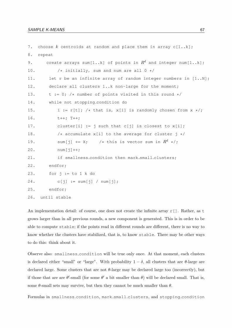
SAMPLE K-MEANS 67
7. choose k centroids at random and place them in array c[1..k];
8. repeat
9. create arrays sum[1..k] of points in Rd and integer num[1..k];
10. / * initially, sum and num are all 0 * /
11. let r be an infinite array of random integer numbers in [1..N];
12. declare all clusters 1..k non-large for the moment;
13. t := 0; / * number of points visited in this round * /
14. while not stopping condition do
15. i := r[t]; / * that is, x[i] is randomly chosen from x * /;
16. t++; T++;
17. cluster[i] := j such that c[j] is closest to x[i];
18. / * accumulate x[i] to the average for cluster j * /
19. sum[j] += X; / * this is vector sum in Rd* /;
20. num[j]++;
21. if smallness condition then mark small clusters;
22. endfor;
23. for j := to 1 k do
24. c[j] := sum[j] / num[j];
25. endfor;
26. until stable
An implementation detail: of course, one does not create the infinite array r[]. Rather, as t
grows larger than in all previous rounds, a new component is generated. This is in order to be
able to compute stable; if the points read in different rounds are different, there is no way to
know whether the clusters have stabilized, that is, to know stable. There may be other ways
to do this: think about it.
Observe also: smallness condition will be true only once. At that moment, each clusters
is declared either “small” or “large”. With probability 1 − δ, all clusters that are θ-large are
declared large. Some clusters that are not θ-large may be declared large too (incorrectly), but
if those that are are θ′-small (for some θ′ a bit smaller than θ) will be declared small. That is,
some θ-small sets may survive, but then they cannot be much smaller than θ.
Formulas in smallness condition, mark small clusters, and stopping condition

SAMPLE K-MEANS 68
will guarantee the following:
Fact: With probability at leat 1− δ, at the end of any round:
• All clusters that are θ-large (with respect to the set of points in x) have been declared
“large”.
• For every a, b such that clusters a and b have been marked “large”, if any point x
whatsoever is assigned to cluster a, then
distance(x, a∗) ≤ (1 + ε) · distance(x, b∗),
where a∗ and b∗ are the centroids that we would get for clusters a and b if we were not
using sampling and running over all x to compute the new centroids.
That is, some points may be classified into different clusters by both the sampling and
non-sampling algorithms. But if a point x is put in cluster a by one and by cluster b
by the other, then x has to be close to the border between a and b, so in some sense
the misclassification is not that bad.
Note that a single misplaced point at one round can change the centroids computed at the
next round. So we do not claim that the solutions computed by the sampling and non-
sampling algorithm look similar in any way, at the end. We just claim that the decisions
(assignments) of the sampling algorithm are almost as good with respect to distances as those
taken by the non-sampling algorithm.
To compute smallness condition:
1. θ′ := θ/3; / * any value θ′ < θ will do * /
2. α := 1− θ′/θ;
3. tmax := 12k · ln(ln(T )/δ)/(θ α2);
4. smallness condition := (t ≥ tmax) but (t− 1 < tmax) ;
Then mark small clusters is as follows: For each cluster j, declare it “small” if
nj <θ + θ′
2k· t,
otherwise declare it “large”.
And stopping condition is a bit more complicated:

SAMPLE K-MEANS 69
1. For each cluster j ∈ {1..k} and each coordinate ` ∈ {1..d} we keep a value εj,` which is
updated at each iteration of the inner loop as follows:
εj,` :=
√2 + 2B/3s[j][`]
· ln ln(T k d)δ
This definition has the property that with probability δ, all s[j][`] are within εj,` of the value
they should have if we added over all points in x, instead of a sample. Let εj stand for the
vector (εj,1, . . . , εj,d).
2. For each i, j, compute farthest(c[i],c[j]), which is the point which is farthest from
c[j] but still within εj of c[i]: for each `, set farthest(c[i],c[j])[`]) to c[i][`] +
εi,` if c[i][`] > c[j][`], and to c[i][`] − εi,` otherwise.
3. Similarly, for each i, j compute closest(c[i],c[j]), which is the point which is closest to
c[j] but still within εj of c[i]: for each `, set closest(c[i],c[j])[`]) to max {c[j][`], c[i][`]−
εi,`} if c[i][`] > c[j][`], and to min {c[j][`], c[i][`] + εi,`} otherwise.
4. Finally, stopping condition is true if
4.1 smallness condition has already occurred (so each cluster is already marked as “large”
or “small”), and
4.2 for every i, j ∈ {1..k}, such that both clusters i and j have been declared “large”,
distance(farthest(c[i], c[j]), (c[i] + c[j])/2)
≤ (1 + ε) · distance(closest(c[i], c[j]), (c[i] + c[j])/2).
Computing this condition directly takes time O(k2 · t) every iteration of the inner loop. Do it
this way for the moment. But I believe there may be more efficient ways to compute it. For
example, at each iteration only one cluster has changed (because only one point is assigned to
it. So maybe we only have to check distances from / to that cluster.

SAMPLE NAIVE BAYES 70
Appendix B
Sample Naıve Bayes
Title: A version of Simple Naive Bayes using sequential sampling - Version 2
From: Ricard G.
To: Joachim N.
Date: June 10th, 2004
Note: We deal with discrete attributes only! No numberic attributes!!
The Simple Naive Bayes algorithm can be written as follows:
1. SimpleNaiveBayes, version 1:
2. / * define some numbers * /
3. N = number of instances
4. A = number of attributes
5. val(a) = number of values of attribute a
6. C = number of classes (= values of the target attribute)
7. V = val(1)+val(2)+...+val(N)+C, total number of values
8. / * create tables for temporary counts, initially all 0 * /
9. create integer classcount[C], a table for holding class counts;
10. create integer count[C][A][val(a)]; / * hope the meaning is clear * /
11. / * count[c][a][v] will hold the number of instances where * /
12. / * class is c and attribute a has value v * /

SAMPLE NAIVE BAYES 71
13. / * compute counts * /
14. for i = 1 to N do
15. get i-th instance, call it x;
16. classcount[class(x)] ++;
17. for a := 1 to A do
18. count[class(x)][a][value of a in x] ++;
19. endfor
20. endfor
21. / * compute prior class probabilities and * /
22. / * conditional probabilities of values to classes * /
23. create float prior[C];
24. create float cond[C][A][val(a)]
25. for c = 1 to C do
26. for a = 1 to A do
27. for v = 1 to val(a) do
28. cond[c][a][v] := (count[c][a][v]+1) / (classcount[c]+val(a));
29. endfor;
30. endfor;
31. prior[c] := (classcount[c]+1) / (N+C);
32. endfor;
33. output the model (prior,cond);
Observe that intuitively, in line 28 we compute Prob(attribute a = v | class = c). That is
(number of instances with a=v and class=c) / (number of instances with class = c). It can be
justified that, because we do not have the true number (over the whole population), but just
a sample, it is convenient to “fake” that we have seen at least one instance with each value
of each attribute. That is why the +1 in the numerator and the +val(a) in the denominator.
This is called “Laplace correction”. In particular, it makes sure that all conditional probabilities
computed are nonzero.
Similarly for the prior probabilities of each class: we must fake that we’ve seen at least one
instance from each class.
The sampling version is similar, except that instead of necessarily going through all the N in-

SAMPLE NAIVE BAYES 72
stances, we pick instances at random from the dataset and stop when some stopping condition
holds. To compute this condition, it is convenient to start “faking” these extra instances from
the start, i.e., when count is created.
The algorithm has three parameters: δ, ε1 and ε2. Their meaning is as follows.
For an instance x and a class c, let M(x, c) be the value assigned to Pr[c|x] by the model obtained
by the sampling algorithm. Let M∗(x, c) be the value assigned to Pr[c|x] by the model built on
all data (that is, without sampling). Then, for all c, with probability 1 − δ (over the choice of
x) we have
(1− ε1) ·M∗(x, c) ≤ M(x, c) ≤ (1 + ε1) ·M∗(x, c)
That is, the difference between the sampling and non-sampling models is at most (multiplica-
tively) ε1.
However, since there may be very small classes and very small conditional probabilities Pr[class =
c ∧ attribute = v] it could take a very very long time to achieve estimations that actually satisfied
this. We introduce ε2 to
prevent the algorithm to take a ridiculously long time because of such very small probabilities.
Formally, we will wait only to make sure that :
1. We have good estimations of Pr[class = c] which are at least as large as ε2/C. Note that the
average Pr[class = c] is 1/C.
2. We have good estimations of Pr[class = c ∧ attribute = v] which are at least as large as
ε2/val(a). Note that the average value of these is is 1/val(a). Also, we do not wait to have good
approximations of these probabilities for classes c which do not pass the test above.
Classes that do not satisfy (1) (resp., counts that do not satisfy (2)) will be called “small”).
So for small classes c or instances with some “small” value attribute = v, we do not claim the
approximation above. There is no formal guarantee that this will not change the classification
error of the newly built model a lot. The hope is that there are few instances where the “winner”
class is really determined by low conditional probabilities.
1. SimpleNaiveBayes, sampling version:
2. inputs ε1, ε2, and δ;
3. / * define some numbers * /

SAMPLE NAIVE BAYES 73
4. N = number of instances
5. A = number of attributes
6. val(a) = number of values of attribute a
7. C = number of classes (= values of the target attribute)
8. V = val(1)+val(2)+...+val(N)+C, total number of values
9. / * create tables for temporary counts, initially all 0 * /
10. create integer classcount[C], a table for holding class counts;
11. create integer count[C][A][val(a)]; / * hope the meaning is clear * /
12. / * count[c][a][v] will hold the number of instances where * /
13. / * class is c and attribute a has value v * /
14. IMPORTANT: initialize all entries of count and classcount to 1,
15. / * compute counts * /
16. t := 0; / * number of iterations * /
17. while not stopping condition do
18. t++;
19. get an instance at random, call it x;
20. classcount[class(x)]++;
21. for a := 1 to A do
22. count[class(x)][a][value of a in x] ++;
23. endfor
24. endfor
25. / * compute prior class probabilities and * /
26. / * conditional probabilities of values to classes * /
27. create float prior[C];
28. create float cond[C][A][val(a)]
29. for c = 1 to C do
30. for a = 1 to A do
31. for v = 1 to val(a) do
32. cond[c][a][v] := count[c][a][v] / (classcount[c]-1+val(a));
33. endfor;
34. endfor;
35. prior[c] := classcount[c] / (N+C);

SAMPLE NAIVE BAYES 74
36. endfor;
37. output the model (prior,cond);
To compute the stopping condition, like in k-means we try to determine that some of the numbers
we try to estimate are “too small”, meaning that it would take too many samples to estimate
accurately. Note that for fixed a and v, if we average Prob[attribute a = v | c] over all classes c
we get average 1/val(a). If an entry looks substantially smaller than that then we will not wait
to have it very well estimated. But we still keep its count. Similarly for classcounts.
The algorithm for computing the stopping condition is then:
1. Let δ′ be δ/(3 · V · ln t)
2. for every c,a,v compute
εc,a,v :=
√3
count[c, a, v]· ln 1
δ′
and for each c compute
εc :=
√3
classcount[c]· ln 1
δ′
Idea: these computations make sure that with high probability, the cond[c,a,v] and prior[c] we
would compute out of these count and classcount are within εc,a,v and εc of the ones we would
get without sampling.
3. for each c which is so far not small: if
(1 + εc) · classcount[c] ≤ t · ε2C
then declare class c “small”.
4. for each c,a,v which is so far not small: if c is small or
(1 + εc,a,v) · count[c, a, v] ≤ (1− εc) · classcount[c] · ε2val(a)
then declare (c,a,v) “small”.
5. Define θ = (ln 2) · ε1/(A + 1).
6. Stop if for all classes c which are not small we have (6.1) θ2 · classcount[c] ≥ 3 ln(1/δ′) and
(6.2) for all counts c,a,v which are not small we have θ2 · count[c, a, v] ≥ 3 ln(1/δ′).
Points 5 and 6 make sure that the value of the resulting model on an instance x will be within
ε1 of the value we would get without sampling, except if some of the conditional probabilities

SAMPLE NAIVE BAYES 75
used to compute the value on x are small, in which case we don’t know. But the idea is that if
class c is winner for x, that is, if the model predicts c as the class with highest probability, no
“small counts” should be used for x and c.
Keeping track of which counts and classcounts are small can be done:
(a) by keeping a separate matrix with boolean entries, of the same sizes as count and classcount
(b) or changing its sign, so a negative count means “small”, and adding an “if” in the algorithm
to do – instead of ++ when computing counts.
(c) other ideas?

BIBLIOGRAPHY 76
Bibliography
[1] Data Mining: Practical Machine Learning Tools and Techniques with Java Implementations.
Morgan Kaufmann Publishers, 2000.
[2] Ruth Dilly. Data mining: An introduction (parallel computer center - queens university
belfast), December 1995.
http://www.pcc.qub.ac.uk/tec/courses/datamining/stu notes/dm book 1.html (June 22,
2004).
[3] Kdnuggets poll: ”data mining tools you regularly use”, May 2003.
http://www.kdnuggets.com/polls/2003/data mining tools.htm (June 25, 2004).
[4] Ricard Gavalda Mestre. Papers by ricard gavalda and coauthors.
http://www.lsi.upc.es/∼gavalda/papers.html (June 22, 2004).
[5] Gordon Paynter. Attribute relation file format (arff), April 2002.
http://www.cs.waikato.ac.nz/∼ml/weka/arff.html (June 8, 2004).
[6] Prof. Dr. K. Coolsaet. Invoer en uitvoer in java (dutch), February 2004.
http://twizz.ugent.be/student/bo/javaio.pdf (June 8, 2004).
[7] Elliotte Rusty Harold. Java I/O. O’Reilly & Associates, 2003-2004.
[8] Weka api (generated documentation).
http://www.cs.waikato.ac.nz/∼ml/weka/doc gui/index.html (June 8, 2004).
[9] Andrew S. Tanenbaum. Structured Computer Organization. Prentice Hall, 2nd edition,
2001.
[10] Prof. Dr. K. Coolsaet. De nieuwe api voor invoer en uitvoer in java (dutch), March 2004.
http://twizz.ugent.be/student/bo/nio.pdf (June 8, 2004).

BIBLIOGRAPHY 77
[11] Ron Hitchens. Java NIO. O’Reilly & Associates, 2003-2004.
[12] Java (tm) 2 platform, standard edition, v 1.4.2 api specification, June 2003.
http://java.sun.com/j2se/1.4.2/docs/api/ (June 23, 2004).
[13] Bill Venners. Inside the Java Virtual Machine. McGraw-Hill, 2nd edition, January 2000.
[14] J. H. Ward. Hierarchical grouping to optimize an objective function. Journal of Amer.
Statist. Assoc. 58: 236-244, 1963.
[15] J. C. Gower. A comparison of some methods of cluster analysis. Biometrics 23: 623-628,
1967.
[16] C.L. Blake and C.J. Merz. Repository of machine learning databases, university of california,
irvine, dept. of information and computer sciences”, May 1998.
http://www.ics.uci.edu/∼mlearn/MLRepository.html (June 27, 2004).
[17] k-means critique.
http://www.clustan.com/k-means critique.html (June 27, 2004).
[18] R.O. Duda and P.E. Hart. Pattern classification and scene analysis. Wiley, 1973.
[19] L.D. Fisher E. Russek, R.A. Kronmal. The effect of assuming independence on applying
Bayes’s theorem to risk estimation and classification in diagnosis. Computers and Biomed-
ical Research 16: 537-552, 1983.

LIST OF FIGURES 78
List of Figures
2.1 Sequence diagram explaining how an Instances object is created . . . . . . . . 16
2.2 (a) Part of Weka’s class diagram, (b) Part of Kiwi’s class diagram. . . . . . . . . 18
2.3 Sequence diagram explaining how to get an Instance from the dataset. . . . . . 20
2.4 Sequence diagram explaining how to remove an Instance from the dataset. . . . 21
2.5 Example of a remove table . . . . . . . . . . . . . . . . . . . . . . . . . . . . . . . 22
2.6 Sequence diagram explaining how to add an Instance to the dataset. . . . . . . 23
2.7 Sequence diagram explaining how to retrieve an Instance with prefetching . . . 24
2.8 Functionality of a 2-bit dynamical prefetch predictor . . . . . . . . . . . . . . . . 25
3.1 Class diagram explaining the design structure for clusterers. . . . . . . . . . . . . 42
3.2 Comparison chart between sampling and non-sampling K-Means with the Syn-
thetic Control dataset . . . . . . . . . . . . . . . . . . . . . . . . . . . . . . . . . 47
3.3 Demonstration chart for the user input variables in Sample K-Means. . . . . . . 49
3.4 Class diagram explaining the design structure for classifiers. . . . . . . . . . . . . 52
3.5 Comparison chart between sampling and non-sampling Naıve Bayes with the
Adult dataset . . . . . . . . . . . . . . . . . . . . . . . . . . . . . . . . . . . . . . 56
3.6 Comparison between sampling and non-sampling Naıve Bayes with the Forest
CoverType dataset. . . . . . . . . . . . . . . . . . . . . . . . . . . . . . . . . . . . 58

LIST OF TABLES 79
List of Tables
1.1 Testing Weka’s capability to handle large datasets . . . . . . . . . . . . . . . . . 5
1.2 Testing number of datasets created during algorithm execution . . . . . . . . . . 6
1.3 Planning of the project . . . . . . . . . . . . . . . . . . . . . . . . . . . . . . . . . 8
1.4 Estimated cost for the working hours . . . . . . . . . . . . . . . . . . . . . . . . . 9
1.5 Total cost estimation . . . . . . . . . . . . . . . . . . . . . . . . . . . . . . . . . . 10
2.1 Performance tests for Weka . . . . . . . . . . . . . . . . . . . . . . . . . . . . . . 37
2.2 Performance tests for Kiwi . . . . . . . . . . . . . . . . . . . . . . . . . . . . . . . 38
3.1 Comparison between sampling and non-sampling K-Means with the Synthetic
Control dataset . . . . . . . . . . . . . . . . . . . . . . . . . . . . . . . . . . . . . 48
3.2 Demonstration for the user input variables in Sample K-Means. . . . . . . . . . . 50
3.3 Comparison between sampling and non-sampling Naıve Bayes with the Adult
dataset . . . . . . . . . . . . . . . . . . . . . . . . . . . . . . . . . . . . . . . . . . 57
3.4 Results of Sample Naıve Bayes with the Forest CoverType dataset. . . . . . . . . 57
4.1 Demonstration of a typical execution flow in Kiwi. . . . . . . . . . . . . . . . . . 61
4.2 Major differences between Weka and Kiwi . . . . . . . . . . . . . . . . . . . . . . 62
4.3 Adjusted planning of the project . . . . . . . . . . . . . . . . . . . . . . . . . . . 63
4.4 Amount of working hours . . . . . . . . . . . . . . . . . . . . . . . . . . . . . . . 63