improve traffic volume estimates from mndot’s regional
TRANSCRIPT

Improve Traffic Volume Estimates from MnDOT’s Regional Traffic Management Center
Taek Kwon, Principal Investigator Department of Electrical Engineering University of Minnesota Duluth
February 2020
Research ProjectFinal Report 2020-02
Office of Research & Innovation • mndot.gov/research

To request this document in an alternative format, such as braille or large print, call 651-366-4718 or 1-800-657-3774 (Greater Minnesota) or email your request to [email protected]. Pleaserequest at least one week in advance.

Technical Report Documentation Page
2. 3. Recipients Accession No.1. Report No.
MN 2020-02
4. Title and Subtitle 5. Report Date
Improve Traffic Volume Estimates from MnDOT’s Regional
Traffic Management Center
February 2020 6.
7. Author(s) 8. Performing Organization Report No.
Taek M. Kwon 9. Performing Organization Name and Address 10. Project/Task/Work Unit No.
Department of Electrical Engineering
University of Minnesota Duluth
271 MWAH, 1023 University Drive
Duluth, MN, 55812
CTS Project# 2017018 11. Contract (C) or Grant (G) No.
(c) 99008 (wo) 251
12. Sponsoring Organization Name and Address 13. Type of Report and Period Covered
Minnesota Department of Transportation Office of Research & Innovation 395 John Ireland Boulevard, MS 330 St. Paul, Minnesota 55155-1899
Final Report 14. Sponsoring Agency Code
15. Supplementary Notes
http:// mndot.gov/research/reports/2020/202002.pdf 16. Abstract (Limit: 250 words)
The Regional Transportation Management Center (RTMC) at the Minnesota Department of Transportation
(MnDOT) deploys a large number of traffic detectors in the Twin Cities’ freeway network and continuously
collects traffic data. While RTMC mainly uses the data for traffic and incident management, the TFA (Traffic
Forecasting and Analysis) office uses the same data for monitoring, forecasting, planning, and reporting of
transportation applications. RTMC provides current and historical volume data generated from its freeway
network, but it does not provide quality information on that data. The objective of this project was to develop a
new tool that can quickly explore the quality of detector data. To allow exploration of data quality, 13 detector-
health parameters were computed using raw volume and occupancy data and then they were stored in a
relational database. The final detector-health system was implemented as a client server-based system, in that a
single server served many remote clients through the Internet. This report provides descriptions of the detector-
health parameters, principles applied, server implementation, client software, and some analyses and application
examples. 17. Document Analysis/Descriptors 18. Availability Statement
Annual average daily traffic, Data quality, Vehicle detectors,
Client server computing, Traffic control centers
No restrictions. Document available from:
National Technical Information Services,
Alexandria, Virginia 22312
19. Security Class (this report) 20. Security Class (this page) 21. No. of Pages 22. Price
Unclassified Unclassified 102

IMPROVE TRAFFIC VOLUME ESTIMATES FROM MNDOT’S
REGIONAL TRAFFIC MANAGEMENT CENTER
FINAL REPORT
Prepared by:
Taek M. Kwon
Department of Electrical Engineering
University of Minnesota Duluth
February 2020
Published by:
Minnesota Department of Transportation
Office of Research & Innovation
395 John Ireland Boulevard, MS 330
St. Paul, Minnesota 55155-1899
This report represents the results of research conducted by the authors and does not necessarily represent the views or policies
of the Minnesota Department of Transportation or the University of Minnesota. This report does not contain a standard or
specified technique.
The authors, the Minnesota Department of Transportation, and the University of Minnesota do not endorse products or
manufacturers. Trade or manufacturers’ names appear herein solely because they are considered essential to this report.

ACKNOWLEDGMENTS
The author would like to thank MnDOT for providing financial and technical support for this research
project. Special thanks go to the Technical Liaison of this project, originally Mark Flinner for inception of
the project ideas, followed by Gene Hicks for carrying on after Mark Flinner’s retirement. Without their
help, this project would not have been successfully started or completed. Thanks are extended to
MnDOT Office of Traffic Forecasting and Analysis (TFA) members Darin Mertig and Christina Prentice for
their direct involvement in trying the detector-health software and providing invaluable feedback.
Thanks are also extended to Doug Lao, at RTMC, for providing assistance on traffic data formats,
incident data, and maintenance data. Special thanks are extended to University of Minnesota-Duluth
graduate students Miles Pierson and Shayan Ali Bhatti for their efforts in many data tests and
verifications.

TABLE OF CONTENTS
CHAPTER 1: INTRODUCTION ...............................................................................................................1
1.1 Background ......................................................................................................................................... 1
1.2 Literature Review................................................................................................................................ 2
CHAPTER 2: DETECTOR-HEALTH PARAMETERS ....................................................................................6
2.1 Detector-Health Parameters .............................................................................................................. 6
2.1.1 Consecutive zero volume (conZeroVol) ....................................................................................... 6
2.1.2 Negative Volume Counts (negVolCnt) ......................................................................................... 6
2.1.3 Consecutive zero occupancy (conZeroOcc) ................................................................................. 7
2.1.4 Negative Occupancy Counts (negOccCnt) ................................................................................... 7
2.1.5 Occupancy lock-on sequence (occLockOn) ................................................................................. 7
2.1.6 Zero-volume on non-zero occupancy (zvolOnOcc) ..................................................................... 7
2.1.7 Volume-over-count (overCnt) ..................................................................................................... 7
2.1.8 Very-high-occupancy (highOcc) .................................................................................................. 7
2.1.9 Constant volume (constVol) ........................................................................................................ 8
2.1.10 Constant occupancy (constOcc) ................................................................................................ 8
2.1.11 Volume on low occupancy (volOnLowOcc) ............................................................................... 8
2.1.12 Correlation Coefficient (CorrCoef) ............................................................................................. 8
2.1.13 Vol/occ ratio (volOccRatio) ....................................................................................................... 9
2.1.14 Conservation-of-vehicles principle ............................................................................................ 9
2.2 Detector-Health-Level Classification ................................................................................................ 10
2.3 COV Application in Station Volume .................................................................................................. 13
2.4 Station Volume Selection RuleS for Computing AADT ..................................................................... 15
2.5 AADT Computation Algorithm .......................................................................................................... 16
CHAPTER 3: Implementation Of Detector-Health System .................................................................. 18

3.1 Overall System .................................................................................................................................. 18
3.2 Database Implementation and Tables .............................................................................................. 20
3.3 Data Processing Steps of the Server Management Software (detHealth_daily) .............................. 25
3.3.1 Step1: Download metro_config.xml ......................................................................................... 25
3.3.2 Step2: Derive three equivalent detector sets for each r_node ................................................ 27
3.3.3 Step 3: Compute all detector-health parameters ..................................................................... 29
3.3.4 Step 4: Apply COV rule-checks for applicable r_nodes ............................................................. 33
3.3.5 Step 5: Adjust HL according to COV tests for r_nodes with main-lane stations ....................... 34
3.3.6 Step 6: Upload health_param and COV_data to the MySQL detectorhealth database ........... 37
3.4 Functions of Server Management Software ..................................................................................... 38
3.5 Client Software: detHealth_app ....................................................................................................... 41
CHAPTER 4: Data Analyses ............................................................................................................... 44
4.1 Histogram Analysis ........................................................................................................................... 44
4.2 Incident Data Analysis ...................................................................................................................... 48
4.3 TESLA Maintenance Data Analysis .................................................................................................... 49
4.4 Detector Replacement: A Known Case ............................................................................................. 49
4.5 Other Examples of detHealth Database Use .................................................................................... 51
CHAPTER 5: Conlusions and Recommendations ................................................................................ 55
5.1 Conclusions ....................................................................................................................................... 55
5.2 Recommendations ............................................................................................................................ 55
REFERENCES .................................................................................................................................... 57
APPENDIX A SAMPLE Histogram Data for Detector-Health Parameters ...............................................1
APPENDIX B Examples of Incident Data Analyses ...............................................................................1
APPENDIX C TESLA Maintenance Log Data Analyses ...........................................................................1

LIST OF FIGURES
Figure 2.1A Pie-Chart Representation of Detector-Health Classification (This pie chart was not generated
from real data, and it is only used for illustration) ..................................................................................... 11
Figure 2.2: Detector-health-level classifier ................................................................................................. 12
Figure 2.3: Equivalent volume relations of a station with presence of entrance and exit nodes between
upstream and downstream stations ........................................................................................................... 13
Figure 2.4: COV relations in an entrance ramp ........................................................................................... 14
Figure 3.1: Client-server implementation of detector-health system ........................................................ 19
Figure 3.2: Numerical and a single-letter representation of Health levels and the three thresholds
defined between four health levels ............................................................................................................ 30
Figure 3.3: Settings window available in detHealth_daily for programming threshold levels ................... 31
Figure 3.4: COV_upgradeDets.20190530.csv ............................................................................................. 36
Figure 3.5: Health level upgrades applied in health_param.20190530.csv for the first four detectors in
Figure 8. ...................................................................................................................................................... 37
Figure 3.6: MySQL script for importing one day of health_param data file ............................................... 37
Figure 3.7: Server management software, detHealth_daily ....................................................................... 40
Figure 3.8: First tab of detHealth_app ........................................................................................................ 41
Figure 4.1: Histograms of ConZeroVol, NegVolCnt, zVolOnOcc and volOccRatio parameters on I-694 2018
data ............................................................................................................................................................. 45
Figure 4.2: Histograms of OccLoackOn, ConstVol, ConstOcc, and volOnLOwOcc parameters on I-694 2018
data ............................................................................................................................................................. 46
Figure 4.3: Histograms of overCnt and highOcc parameters on I-694 2018 data ...................................... 47
Figure 4.4: Consecutive zero volume plot of detector 472 for the period 1-1-2015 to 31-12-2016 .......... 50
Figure 4.5: Daily detector volume total for the period 1-1-2015 to 31-12-2016 ....................................... 51
Figure 4.6: Retrieval of a Continuous Count (CC) station #309 .................................................................. 52
Figure 4.7: Six-month volume data retrieval of temporary detector T35103 ............................................ 53

Figure 4.8: Six-month negVolCnt retrieval of temporary detector T35103 ................................................ 53
Figure 4.9: 30-Second volume and occupancy plots for detector T35103 on April-26-219 ....................... 54
LIST OF TABLES
Table 1: Vol/Occ Ratio Thresholds for 30 Second Loop Data ....................................................................... 9
Table 2: Column Description of health_param Table ................................................................................. 21
Table 3: Column description of “cov_data” Table in detectorhealth Database ......................................... 24
Table 4: Detector Category ......................................................................................................................... 27
Table 5: COV Defines Table ......................................................................................................................... 29
Table 6: Column Headings of Health Parameter Thresholds ...................................................................... 30
Table 7: Column Headings and Data Types of COV_diffRatio.csv Table ..................................................... 35

LIST OF ABBREVIATIONS
MnDOT Minnesota Department of Transportation
FHWA Federal Highway Administration
AASHTO American Association of State Highway and Transportation Officials
RTMC Regional Transportation Management Center
TMC Traffic Management Center
TFA Traffic Forecasting and Analysis
AADT Annual Average Daily Traffic
CC Continuous Count
CSV Comma Separated Values
SC Short-Duration Count
GUI Graphical User Interface

EXECUTIVE SUMMARY
The Regional Transportation Management Center (RTMC) at the Minnesota Department of
Transportation (MnDOT) manages the Twin Cites’ (St. Paul and Minneapolis) freeway network and
aggregates traffic data from a large number of vehicle detectors (about 7,830 detectors in 2019 and
growing every year). Two types of vehicle detectors are mainly deployed, inductive loop detectors and
microwave radar detectors. RTMC saves detector data consisting of volume, occupancy, and speed
(when available) at a data rate of every 30 seconds from all detectors. MnDOT offices, such as Traffic
Forecasting and Analysis (TFA), use this data for Federal Highway Administration (FHWA) reporting,
traffic forecasting, and multiple planning applications.
One of the MnDOT TFA office’s challenges in using RTMC detector data has been unavailability of quality
information. Knowing which detectors have been producing high-quality data is critical for TFA, since
choosing a set of good detectors leads to better or higher-quality design outcomes. For example, a
continuous count (CC) station requires a set of detectors that provide good-quality data throughout the
entire year, from which parameters like seasonal adjustment factors are more accurately computed.
Consequently, quality control of traffic data has been an important issue to TFA. FHWA has also
emphasized the same issue for many years, evidenced by TMG-2016 Section 2.6, which specifically
states, “The TMG recommends that each agency improve the quality of reported traffic data by
establishing quality assurance processes for traffic data collection and processing.”[1] This project was
created to develop a tool for TFA analysts to quickly explore RTMC detector data and identify bad or
good detectors for a given period.
This project was started by reviewing an extensive list of literatures available on traffic detector
diagnostic algorithms and erroneous data detection techniques, and then 13 diagnostic parameters
were adopted. These parameters, which are named detector-health parameters, form the basis for
quality control in this project, and they are all derived from raw 30-second detector volume and
occupancy data. The parameters are computed every day for each detector and then stored in a
relational database. The same parameters for each day are also fed into a classifier that outputs a
health-level of the detector for the day. To simplify quality representation, four health levels were
defined, which are: healthy, tolerable, impaired, and nonfunctional. Detectors in the healthy class were
recommended for vehicle counting programs while the detectors in the tolerable class were
recommended only if no healthy class detectors were available for the same location. The detectors in
impaired or nonfunctional classes were not recommended for counting applications and considered
targets for maintenance operations.
The final detector-health system was implemented as a client-server system, in which a single server
supplies data to many remote clients through the Internet. The server contains a relational database,
and a software tool called “detHealth_Daily.exe” that computes and loads detector-health parameters
to the detector-health database. This software tool connects to a data server called IRIS (Intelligent
Roadway Information System) managed by RTMC, obtains raw volume and occupancy data for each
detector, and then computes all detector-health parameters. For the relational database engine, a free
version of MySQL is used. Currently, only one client program called “detHealth_App” is available, which

is installed on the user’s personal computer. This application software provides detector-health
classification in a pie chart per day, retrieval of health parameters, parameter visualization, station AADT
computation, etc.
This report includes few data analysis examples that were part of testing and development of the
detector-health system (summarized in Chapter 4). Histograms of all detector-health parameters on
interstate highway I-694 were computed, plotted, and analyzed to understand the frequency of
occurrence. In histograms, most parameters exhibited an exponential distribution with a heavy
concentration in the first few bins, which suggests that a majority of detectors were healthy for most of
the time.
RTMC maintains an incident database that stores reported incidents on the Twin Cities’ freeway
network. Part of this data, which was provided to the research team, was a collection of incident data
from the I-694 and I-94 interstate highway systems for the period, from January 1, 2015, to December
31, 2016. In this data, RTMC classified incidents into four categories, which were stall, roadwork, hazard,
and crash. Each incident was recorded as a single database record and its location was specified using
latitude and longitude but without detector IDs. Since incidents were not directly tied to detector IDs,
the research team had to study all potential detectors near the incident location and then figure out
how each incident affected the corresponding detector data. It was found that roadwork and hazard
incidents increased consecutive zero-volume counts, but crash and stall incidents did not noticeably
affect zero-volume counts or daily traffic volumes.
TESLA is a legacy RTMC maintenance logging system that recorded loop maintenance work orders.
RTMC transitioned to a new maintenance logging system called TAMS in the fall of 2016 but provided
the research team with the old TESLA data for 2015 and 2016 for study. As the basic methodology of
investigating this data in relation to detector-health parameters, all stations on I-694 and I-94 were
investigated. For all detectors in every station, whether they have had a record or records in the TESLA
log from January 2015 to December 2016 was checked. If a maintenance record was found, then all
detector-health parameters for that station were investigated. The research team found that detector
repairs resulted in a sequence of event patterns. More specifically, all detectors in the station of repair
event typically stopped producing data for few days before the repair, followed by a large number of
negative volume counts for a few days, and then a normal pattern of traffic data was returned.
In conclusion, this project was born out of the need for quality information on the detector-volume data
provided by RTMC. Since RTMC does not provide quality information on its traffic data, the research
team had to create a wide range of detector-health parameters to use as a quality measure. A database
of these health parameters provided a new tool for exploring quality information of detectors. During
the project period, TFA reported that this new tool was used on several occasions and was effective in
exploring reported problems of some continuous or short-duration count stations, as well as for a
specific detector.

1
CHAPTER 1: INTRODUCTION
1.1 BACKGROUND
Modern transportation systems rely heavily on many traffic sensors and the data they generate. Traffic
management centers (TMCs) in major cities across the U.S. are one example; they typically manage tens
of thousands of traffic detectors installed on their city’s freeways. The data produced from such a large
system are often referred to as ITS (Intelligent Transportation Systems) generated data, because they
are part of a large-scaled, sophisticated ITS network deployed throughout major cities. State
transportation departments in planning and traffic forecasting offices use this available data for
transportation monitoring, forecasting, planning, and reporting applications [1].
ITS-generated traffic data are generally sampled at a higher time resolution than that of traditional
traffic counting devices (such as pneumatic tube counters or piezo-sensor stations) because they are
mainly used for real-time traffic and incident managements. Data are typically recorded every 15 to 30
seconds. Due to a huge number of detectors deployed in TMC-managed freeway networks, it is often
hard to maintain all of them to work in their full capacity, and thus some bad detectors are likely to be
present in the system. The causes could be hardware malfunctions, road constructions, communication
failures, power-supply problems, calibration errors, etc. Since a TMC’s mission is mainly in real-time
traffic management, once the real-time data has been used for applications such as ramp metering or
incident managements, the quality of past data is of less concern and their operations simply move on
to the next phase. However, if the same data are used for transportation planning applications, accuracy
of past traffic data, especially volume, becomes extremely important, because it can affect the
outcomes of analyses, projections, or designs. Although a huge amount of traffic data is available from
TMCs, information on which portion of the data is good or bad is rarely available. Therefore, there is a
need to measure, label, and assure the quality of data before they are used in transportation
applications.
In Minnesota, the Regional Transportation Management Center (RTMC) within the Minnesota
Department of Transportation (MnDOT) manages freeway traffic and incidents in the Twin Cites (St. Paul
and Minneapolis) and aggregates data from about 7,830 detectors (in 2019 and this number grows
every year) installed on the cities’ freeway network. Two types of detectors have mainly been deployed,
which are loop detectors and microwave radar detectors. RTMC daily saves the detector data consisting
of volume, occupancy, and/or speed if it is available, at a data rate of every 30 seconds from all
detectors. Within MnDOT, offices involving transportation planning and forecast, such as Traffic
Forecasting and Analysis (TFA), use this data to produce short-duration and continuous count data for
various Twin Cities’ freeway locations. However, one of the major issues to TFA has been how to know
(or discover) a set of good detectors without availability of data quality information. This project was
created to improve quality of volume data by utilizing some form of detector quality parameters
computed from 30-second volume and occupancy data available from RTMC. A strategy developed in
this project was to create a database for detector-health parameters for each detector per day.

2
It should be mentioned that the effort of establishing a quality-control process at MnDOT TFA goes in
parallel with the FHWA’s efforts in introducing quality control into traffic data collection and processing.
TMG-2016 (Section 2.6) states, “The TMG recommends that each agency improve the quality of
reported traffic data by establishing quality-assurance processes for traffic data collection and
processing.” [2]
1.2 LITERATURE REVIEW
A large volume of research work has been done in the area of understanding faults in loop detectors and
detecting consequential errors from the data. This section reviews literatures available on traffic
detector diagnostic algorithms and erroneous data-detection techniques. Major sources used for this
literature review were from the Transportation Research Record on-line database and Google scholar
searches.
Although numerous vehicle detection technologies, which include magnetic sensors, magnetometers,
inductive loop detectors, video image processors, microwave radars, ultrasonic, acoustic, passive
infrared sensors, etc., have been developed and commercially available for many years, inductive loop
detectors have been by far the most widely used vehicle sensing technology in modern traffic control
systems (Traffic Detector Handbook [2]). Similarly, traffic detectors in the Twin Cities’ freeway network
managed by MnDOT RTMC also consist predominantly of inductive loop detectors. Therefore, this
literature review focuses on loop detector diagnostics, but many of the same techniques could be used
in other types of sensors.
In general, loop detector diagnostic approaches are classified into two levels: microscopic and
macroscopic, initially coined by Jacobson et al. [3]. Microscopic-level diagnostic tests concern individual
vehicle actuation signals or diagnostic indicators output by detector electronics in the field cabinet.
Macroscopic-level diagnostic tests, on the other hand, refer to quality-control algorithms executed at
TMCs after the data have been aggregated from field sensors.
A comprehensive treatment in microscopic-level information on inductive loop detectors can be found
from the Traffic Detector Handbook [2]. It includes detailed descriptions of the underlying physics of
inductance changes by a vehicle passage, proper installations of loop wires and lead-in cables, electronic
units (detector board), acceptance tests, maintenance, and standards. This reference mainly provides
information on basic failure tests at a control cabinet where individual loop detectors are connected.
The tests include open/grounded-loop tests, presence/pulse mode tests, crosstalk detection tests, and
sensitivity setup checks. An example of this type of basic loop signal test can be found from the methods
developed in California, which established loop-detector installation acceptance criterion and
maintenance techniques, as early as in mid-1970s [4].
A large volume of work on microscopic-level loop diagnostics has been developed at the Berkeley
Highway Laboratory (BHL) that uses vehicle actuation signals (event data) in the detector card [5]. Loops
operate in presence mode for freeway operation applications. That is, they turn on and stay on as long
as a vehicle is present on the loop detection zone. This actuation signal, consisting of on-times and off-
times, is sampled at 60 Hz through a controller such as model 170. What is distinctive at BHL was that

3
the on-time/off-time event data were transferred to the central sever located in their TMC and the
event data was then used for developing loop-detector diagnostic algorithms [5]. The main advantage of
tapping into this on-time/off-time vehicle actuation signal is fidelity available for individual vehicle
measurements. For example, Chen and May [6] examined individual vehicle on-time of single loops
against the statistical vehicle on-time data and determined validity of the detector operations. Their
approach was sensitive to additional errors such as pulse breakups, where a single vehicle registers
multiple actuations. Loop diagnostics utilizing on-time of dual loops was devised by Coifman [7]. The
assumption he used was that at free-flow traffic, the on-times from the two loops should be virtually
identical regardless of vehicle length. Loop errors were reported when two on-times differed over a
preset threshold level. Coifman and Dhoorjaty [8] extended this result to include several more detector-
validation tests such as a headway versus on-time ratio test, feasible range of vehicle lengths test,
cumulative distribution of vehicle lengths, etc. Another interesting work was done by Lee and Coifman
[9], in which they devised an algorithm that could detect pulse breakup errors. Diagnosis of pulse
breakup was possible by examining short off-times and then differentiating between pulse breakups and
tailgating. Following BHL studies, a similar detector-event data-collection system was implemented by
the TransNow research team at the University of Washington (UW) [10].
In loop detectors, crosstalk is typically caused by inductive or capacitive coupling between closely placed
loops or closely spaced lead-in wires operating at similar frequencies and leads to false detection and
counting [2]. The Traffic Detector Handbook [2] suggests detailed instructions on how to avoid crosstalk
errors by selecting different frequencies and carefully wiring the lead wires, but it does not provide
information on how to detect them. A systematic approach in detecting crosstalk from loops proposed
by Ernst et al. [11] developed a crosstalk detection algorithm based on a spectral analysis of vehicle
inductance signatures in the frequency domain computed by Fast Fourier Transform (FFT).
Another type of detector error not discussed frequently but important is the segmentation error.
Because loop detector event (actuation) data requires extra storage and bandwidth, controllers in a
cabinet typically aggregate data in a preset interval, such as 30 seconds, into two values, volume and
lane occupancy, which are then sent to TMC. A segmentation error may occur when a vehicle is present
on the loop when the current interval terminates. In this case, the vehicle is counted toward the
following interval, but part of its scan counts for occupancy are mistakenly assigned to the current
interval. This incorrect count of scan in computing occupancy is referred to as a segmentation error. Yu
et al. [12] developed a segmentation error detection algorithm based on loop-detector event data and
was able to use that information to improve speed estimation from single loop detectors. They found
that more than 15% of intervals are, in general, contaminated by segmentation errors [12].
Until now, microscopic-level or control-cabinet level loop-diagnostic techniques have been reviewed.
Next macroscopic-level diagnostics techniques are considered, in which detectors are diagnosed using a
large amount of volume and occupancy data collected at a TMC. Macroscopic algorithms may be further
divided into algorithms based on a single location analysis and a system-level analysis of multiple
locations. As an example of single location analysis, Jacobson et al. [3] devised a diagnostic algorithm
based on an “acceptable region” in the k-q plane, declaring the data good if they fall inside the
acceptable region. The boundaries of the acceptable region are defined by a set of parameters, which

4
are calibrated from historical data. Cleghorn et al. [14] extended the work of Jacobson et al. by
tightening the upper bound for the k-q ratio through the application of traffic-flow theory. Chen et al.
[14] devised an algorithm based on daily statistics of detector error conditions, which is basically
another way of testing acceptable regions of the k-q plane. More specifically, they tested daily statistics
of four conditions: (1) occupancy and flow are mostly zero, (2) non-zero occupancy and zero flow, (3)
very high occupancy, and (4) constant occupancy and flow. In addition, they devised an imputation
algorithm for missing data points. Another algorithm for testing a single location was developed by
Kwon and his students, which tested 10 parameters through a large decision tree [15].
The second type of macroscopic-level diagnostic is based on spatial relations of traffic flow at the system
level, involving multiple detector stations. A detector station here refers to a control cabinet that
aggregates and processes loop signals from all lanes at that location and transfers the aggregated data
(volume and occupancy) to TMC. The most frequently applied principle for system-level analysis is called
the conservation-of-vehicles (COV) principle [16]. It states that, if the total number of vehicles counted
by two consecutive detector stations is observed over a period, the difference in the cumulative counts
at any time should not exceed the number of vehicles that can be accommodated in that length of the
road under the jam density [17]. When the traffic volumes of two consecutive stations violate this
principle, the cause is under or over counts of vehicles in the stations involved. Vanajakshi and Rilett
successfully applied this principle in freeway traffic to diagnose bad loop-detector data [17]. Wall and
Daily [20] used the same principle to adjust highway traffic volumes. Weijermars and Van Berkum [18]
further extended and applied the COV principle in detecting invalid traffic data produced by single loop
detectors at signalized intersections. In Minnesota, Kwon and MnDOT applied the COV principle in
determining equivalent detector sets referred to as primary, secondary, and tertiary detector sets for
computing annual average daily traffic (AADT) of a location [19]. In this approach, when errors were
detected from the primary detector set, AADT was computed using the secondary detector set; when
errors were present in the secondary set as well, AADT was computed from the tertiary detector set. If
all three sets failed, the current data for the corresponding station were thrown away. This approach
was implemented and used by MnDOT.
In California, macroscopic-level diagnostics were applied through a large data aggregation system called
PeMS (Performance Measurement System) [21]. With so much detector data (over 25,000 loops)
collected to one location, many loop detector locations were mislabeled as an error in lane direction.
Kwon et al. [22] developed an approach that can detect incorrect configuration information about the
loop locations. Their method relies on the fact that flow, occupancy, or speed measurements between a
pair of loops that are spatially close must show higher correlations than when they are farther apart.
They found that 15.6% of loops had incorrectly assigned labels on the stretch of road they studied.
Another interesting effort was introduction of a dashboard concept into TMC operations. Hranac and
Petty [23] proposed digital dashboards representing detector health within the framework of PeMS. A
dashboard is a collection of graphical visualizations of key metrics for decision makers. For example, it
could display the percentage of bad detectors in a district, such as 65% of detectors are good and 34% of
detectors are bad. The user can then drill down into the data to discover more details and validate the
data interpretation.

5
Many loop-data screening tests at a macroscopic level are available as summarized above [17-23]. Most
of them focus less on identification of the maintenance-required detectors and more on imputing or
correcting the bad data. One of the interesting approaches might be integrating many of the studies and
practices available into a single integrated solution. This research attempts to identify and integrate
many of the past diagnostic tools into one integrated system to develop a quality-control software tool.

6
CHAPTER 2: DETECTOR-HEALTH PARAMETERS
This chapter describes detector-health parameters and health-level classification developed as a
representation of quality in this project. All diagnostic parameters are integrated into a single database,
and then a system level algorithm is explored using application of the Conservation-Of-Vehicles (COV)
principle.
2.1 DETECTOR-HEALTH PARAMETERS
The raw data available from RTMC detectors are 30-second volume and occupancy data. Occupancy
data are not available for all detectors but volume data are. Each parameter presented in this section
may be classified into one of the four cases: (1) computed from volume data only, (2) computed from
occupancy data only, (3) computed using the relationship between volume and occupancy, and (4)
spatial relation of volume data. Most of the parameters described below are a collection of well-known
detector diagnostic parameters in literatures surveyed in Section 1.2. Some parameters are unrelated to
detector-health measure but included for future utility of the database. Each parameter is described
with its definition and the actual short name used in the database. The short name was the database
column name and is shown as italic letters inside the corresponding parenthesis.
2.1.1 Consecutive zero volume (conZeroVol)
This value is an integer and represents a total number of 30-second time slots comprising a collection of
consecutive zero volumes for 10 or more minutes. More specifically, there are 2,880 30-second time
slots in a day (24 hours), and conZeroVol is obtained by counting the number of time slots only if zero
volumes consecutively occur and it lasts longer than 10 minutes (i.e., zero volumes are found from more
than 20 consecutive 30 second time slots). If the duration of consecutive zero-volumes is less than 10
minutes, it is ignored. A small conZeroVol value may not directly correlate to a faulty condition but when
its value becomes very large, it indicates a potential problem in the sensor or system. For example, if a
detector has consecutive zero volumes for more than 24 hours, it is highly likely that the detector is
experiencing a faulty condition or a lane closure (construction or special event). This parameter has
been used by MnDOT as a quality factor in the past, and it was particularly used as one the main
measures to replace primary set volumes with secondary or tertiary equivalent volumes [19].
2.1.2 Negative Volume Counts (negVolCnt)
Total number of 30-second time slots with negative volumes. Volume values cannot be a negative
number, but it is often used by the system to indicate an error condition. RTMC also places a negative
volume number in 30-second time slots if an error condition was discovered in that slot.

7
2.1.3 Consecutive zero occupancy (conZeroOcc)
Total number of 30-second time slots comprising a collection of continuous time spans with consecutive
zero occupancies for 10 or more minutes. The same reasoning described in the consecutive zero
volumes is applicable to consecutive zero occupancies.
2.1.4 Negative Occupancy Counts (negOccCnt)
Total number of 30-second time slots with negative occupancies. Occupancy values cannot be a
negative number, but it is used by the system or detector to indicate an error condition.
2.1.5 Occupancy lock-on sequence (occLockOn)
Total number of 30-second time slots comprising a collection of time spans of consecutive occupancy
lock-on conditions (i.e., 99<occupancy≤100) for 10 or more minutes. Occupancy values greater than 99
percent are possible in real-world traffic under congestion, but lasting many long hours (such as
consecutive 24 hours) imply an error condition.
2.1.6 Zero-volume on non-zero occupancy (zvolOnOcc)
Total number of 30-second time slots in which zero-volumes were detected on non-zero-occupancy.
Ideally, zero volume should only exist under zero occupancy within each time slot. However, zero
volume on non-zero occupancy may occur if a partial vehicle presence was captured at the end of the
current time slot, and then the same vehicle is again captured and counted in the subsequent time slot.
This problem is often referred to as a segmentation error [12]. If zero volumes persist on non-zero
occupancies, a faulty condition in the detector may be the cause.
2.1.7 Volume-over-count (overCnt)
Total number of 30-second time slots in which volume is greater than 25 but less than 128 (25<vol<128).
The theoretical limit of a single-lane volume for 30 seconds is around 25. If a 30-second volume exceeds
this limit, it is likely caused by a fault such as mutual coupling in which vehicles in adjacent lanes are
counted.
2.1.8 Very-high-occupancy (highOcc)
Total number of 30-second time slots with occupancy greater than 35%. This parameter correlates to
detection of congestion, but it may provide additional information when it is used along with other
parameters. If highOccs are present for a long period, it may be caused by a faulty condition in detector.

8
2.1.9 Constant volume (constVol)
Total number of consecutive 30-second time slots in which volume values remain constant in the range
(0<vol<128) for 10 or more minutes. In normal traffic conditions, volume counts at consecutive time
slots rarely repeat, except for zeroes in low traffic hours. If a non-zero constant volume repeats for more
than 10 minutes from a detector, it is likely caused by a faulty condition in the detector.
2.1.10 Constant occupancy (constOcc)
Total number of consecutive 30-second time slots in which occupancy values remain constant in the
range (0.2<vol<100) for 10 or more minutes. The same reasoning described in the constant volume is
applied to constOcc.
2.1.11 Volume on low occupancy (volOnLowOcc)
Total number of 30-second time slots in which volume is greater than one when occupancy is in the
range occ≤0.2%. In a 30-second time slot, 0.2 percent occupancy can be measured on a 6x6 feet loop by
a single vehicle passage of one feet in length with 80 mph speed. Therefore, an occupancy that is less
than 0.2 percent is unrealistic, and it is only possible by a passage of a segment of a vehicle [12]. This
condition occurs when vehicle on-time is present between two adjacent time slots. Such a low
occupancy should not be counted as a complete vehicle since it is a fragment of a vehicle. Existence of
multiple time slots with volumes greater than one when occ≤0.2% indicates a potential faulty condition
in that detector.
2.1.12 Correlation Coefficient (CorrCoef)
The Correlation Coefficient (CorrCoef ) between volume and occupancy of a detector indicates a degree
of linearity between them, and it is computed using the following formula.
𝐶𝑜𝑟𝑟𝐶𝑜𝑒𝑓 =∑ [(𝑉𝑜𝑙(𝑖)−𝑉𝑜𝑙𝑎𝑣𝑔)(𝑂𝑐𝑐(𝑖)−𝑂𝑐𝑐𝑎𝑣𝑔)]2879
𝑖=0
√∑ (𝑉𝑜𝑙(𝑖)−𝑉𝑜𝑙𝑎𝑣𝑔)22879𝑖=0 √∑ (𝑂𝑐𝑐(𝑖)−𝑂𝑐𝑐𝑎𝑣𝑔)22879
𝑖=0
(1)
where i is an index of 30-second time slots, occ(i) is the occupancy at the ith time slot, vol(i) is the
volume of the ith time slot, and subscription avg indicates an average. If CorrCoef is close to one, it
means that the relation between volume and occupancy is almost perfectly linear, which is only possible
by a “pulse mode” in a loop detector card. Pulse mode does not affect volume counts but affects speed
estimates. Therefore, this parameter is included mainly for detection of pulse modes in loop cards.

9
2.1.13 Vol/occ ratio (volOccRatio)
The volume and occupancy ratio (vol/occ) of a 30-second time slot on a healthy detector should stay
inside the theoretical acceptable bounds. This theory was originally developed by Jacobson et. al [3] and
adopted in this research as one of the detector-health parameters. The vol/occ ratio for a 30-second
data follows the relation [3],
vol/occ = (u * g)/120 (2)
where vol is the 30-second volume, and occ is the 30-second occupancy in percent, u is speed in mph,
and g=K/(vehicle length + detector length) where K is a conversion factor. Simply speaking, g is a
parameter that makes a speed estimation possible using only volume and occupancy, and thus it is a
function of vehicle length. At RTMC, this value is called field length. Table 1 shows the acceptable ranges
of vol/occ under four different ranges of occupancies. It was constructed by only modifying the speed
limits (min and max speeds) of the original table derived by Jacobson et. al [3] to adapt to speed limits of
the TC freeways but using the same g values. If a vol/occ ratio is outside this range, the data is
considered erroneous.
Table 1: Vol/Occ Ratio Thresholds for 30 Second Loop Data
Occupancy Ranges (%)
0.2 – 7.99 8.0 – 25.99 26.0 – 35.99 36.0+
Min g 2.322 2.024 1.754 .980
Max g 3.832 2.526 2.462 1.868
Min speed (mph) 24.22 18.63 8.69 6.83
Max speed (mph) 95 88 50 40
Min Vol/Occ .469 .314 .129 .056
Max Vol/Occ 3.033 1.852 1.026 .623
2.1.14 Conservation-of-vehicles principle
The conservation-of-vehicles (COV) principle is stated as: “the total number of vehicles counted by the
upstream station should be counted by the downstream station at some future point in time if there are
no exits and entrances between them.” [16]
Consider a pair of upstream and downstream stations on the same road with all detectors in the same
direction, and no exits or entrances exist between them. The configuration of this pair of stations must
satisfy the conservation-of-vehicles principle since there are no entrances or exits between them. Let
the cumulative difference of volumes at the k-th 30-second time slot between the pair be denoted D(k).
Then the differences are:
𝐷(𝑘) = 𝑇𝑢(𝑘) − 𝑇𝑑(𝑘 + 𝜏) 𝑘 = 1 … 𝐾 − 𝜏 (3)

10
where Tu is the total volume at upstream, Td is the total volume at downstream, and τ is the time lag to
catch the vehicles coming from upstream. If D(k) increases over time, it implies that some vehicles
counted at upstream are not counted at downstream. If D(k) decreases over time, it implies that some
vehicles not counted at upstream are counted at downstream. If D(k) is zero or near zero, it implies that
vehicles are counted at the same time from both stations, which also indicates an error condition.
A normalized difference ratio (diff_ratio) of volumes between a pair of stations is measured as:
𝑑𝑖𝑓𝑓_𝑟𝑎𝑡𝑖𝑜(𝑣1, 𝑣2) = |𝑣1 − 𝑣2|/(𝑣1+𝑣2
2) (4)
where v1 and v2 are the cumulative station volumes for a single day ending at midnight.
If this ratio is very small such as less than 0.01 when it is computed for the entire day (midnight-to-
midnight), it indicates that the station traffic volumes between the two stations obey the COV rule. This
in turn suggests that all detectors in both stations are working correctly since it is extremely hard to
satisfy COV if any of the detectors in the two consecutive stations are not properly functioning.
Therefore, COV tests are preferably used to detect a set of healthy detectors. This project computes
volumes at three consecutive, equivalent stations and then compares them using diff_ratio in Eq. (4) to
determine a satisfactory condition of COV.
2.2 DETECTOR-HEALTH-LEVEL CLASSIFICATION
This project defines four levels of detector health: healthy, tolerable, impaired, and nonfunctional. A
graphical representation may be expressed using a simple pie chart as shown in Figure 1. Such a chart
could quickly show or summarize the health status of the whole detectors in a system, from which
further information may be queried upon selecting one of the classes, similarly to the dashboard
concept developed in [23].

11
Figure 2.1 A Pie-Chart Representation of Detector-Health Classification (This pie chart was not generated from
real data, and it is only used for illustration)
Healthy60%
Tolerable10%
Impaired10%
Nonfunctional20%
In this classification scheme, detectors in Healthy class are more desirable for vehicle counting
programs, since the detectors in Healthy category provide the highest quality of counting data.
Detectors in Tolerable should be used for counting only if the detectors in Healthy class are no longer
available for the given location.
The detectors in Impaired or Nonfunctional are targets for maintenance operations and not
recommended for vehicle counting programs. Nonfunctional class is assigned to detectors that are
completely broken and do not generate any useable data. These detectors should be considered as the
highest priority targets for maintenance. Detectors in Impaired class generate data that may include a
large portion of them missing or erroneous, and thus considered not accurate enough for use in vehicle
counting programs.
The health level of a detector is determined using a classifier algorithm that takes in N acceptance tests
using the parameters described in Section 2.1. Figure 2 illustrates the concept of this classifier.
Presently, 12 parameters are fed into the algorithm, and threshold levels set by user (user
programmable) determines the classification.

12
Figure 2.2: Detector-health-level classifier
Detector Health-Level Classifier
Test 1
Test 2
Test N
HealthyTolerable
Impaired
Nonfunctional

13
2.3 COV APPLICATION IN STATION VOLUME
The COV principle described in Section 2.1.14 could be applied between two consecutive stations, even
if entrances and/or exits between them may exist. Consider Figure 3 that has one entrance and one exit
between each pair of two consecutive stations. The station in the middle is named Cur_Sta (current
station), and its relations to upstream is called Up_Sta (upstream station) and downstream to Dn_Sta
(downstream station). A simple COV rule is that entrances add while exits reduce the total volume at the
downstream station. Suppose that we wish to estimate Cur_Sta volume in terms of the Up_Sta volume,
and call this volume Equiv_Up_Sta_vol. Then, Equiv_Up_Sta_vol is computed by adding the Entrance_1
volume and subtracting the Exit_1 volume from the Up_Sta volume, i.e., the Eq. (5) holds for cumulative
volumes ending at midnight.
Equiv_Up_Sta_vol = Up_Sta_vol + Entrance_1_vol – Exit_1_vol ≈ Cur_Sta_vol (5)
Similarly, the equivalent downstream volume (Equiv_Dn_Sta_vol ) can be calculated using current
station volume as:
Equiv_Dn_Sta_vol = Dn_Sta_vol - Entrance_2_vol + Exit_2_vol ≈ Cur_Sta_vol (6)
Figure 2.3: Equivalent volume relations of a station with presence of entrance and exit nodes between upstream
and downstream stations
Entrance_1Entrance_2
Exit_1Exit_2
Cur_StaUp_Sta Dn_Sta
This leads to a condition for healthy station as:
Cur_Sta_vol ≈ Equiv_Up_Sta_vol ≈ Equiv_Dn_Sta_vol (7)

14
The basic reasoning for using Eq. 7 as the acceptance condition for a healthy station is that, if one or
more malfunctioning detectors exist in any of the stations under test, it will affect the total volume of
the station and is unlikely to hold COV relations on three equivalent stations. Reviews on actual RTMC
traffic data showed that less than 1 percent of differences exist when all detectors involved are working
correctly. When detector errors exist, the differences were typically higher than 5 percent.
The COV principle may also be applied to detectors in an entrance ramp. Figure 4 illustrates multiple
types of detectors installed in a typical entrance ramp on the Twin Cities’ freeway network. This
particular example has a passage detector (labeled P), a bypass detector (labeled B), a merge detector
(labeled M), and two queue detectors (labeled Q). Queue detectors are used to detect if the vehicles
queued at an entrance ramp are stretched beyond the queue detectors or not. A bypass lane allows
bypass of high-occupancy vehicles (HOVs) where a B detector is placed. Merge detectors count all
vehicles entering the highway from the entrance node where the M detector was installed, resulting in
equal to the sum of traffic volumes in passage and bypass lanes. Therefore, the equivalency relation for
daily volumes of detectors in an entrance ramp is given by:
Vol(all Q) ≈ Vol(P + B) ≈ Vol(M) (8)
Figure 2.4: COV relations in an entrance ramp
Station
Q
P
B
M
Q
X
Main Lane Detectors
Station Station
Exit
Entrance
Main Lane Detectors

15
Eq. (8) describes that volume sum of all Q detectors or M detector should be equal to the volume sum of
P and B detectors. This relation was used to identify good detectors in entrance ramps in a similar
manner as the COV rules applied on consecutive stations.
It should be noted that exit ramps in the Twin Cities’ freeway network do not have redundant detectors
installed, thus the COV principle cannot be applied in exit ramps. It is also important to note that the
COV principle does not reveal information on which detector is bad or good, but it gives information on
which station contains one or more bad detectors. Because of this limitation, it is only used for
identifications of good stations.
2.4 STATION VOLUME SELECTION RULES FOR COMPUTING AADT
For each station, three equivalent station volumes are daily available for computing AADT [24] as
illustrated Figures 3. Therefore, there must be a rule for choosing a station volume from the available
three stations. This section describes the selection rules developed and implemented in this project.
Let the daily station volume be denoted for i-th station on day k as Sta_vol(i, k). Define the equivalent
upstream and downstream volumes as Sta_vol(i+1, k) and Sta_vol(i-1, k), respectively, i.e.,
Sta_vol(i+1, k) = equivalent upstream station volume of station i on day k,
Sta_vol(i, k) = current station volume of station i, on day k,
Sta_vol(i-1, k) = equivalent downstream station volume of station i on day k,
When station volumes are computed, a missing percent of the daily volume is also computed by dividing
the total number of 30-second time slots with missing values. For example, if volume data in a day
include 360 missing slots, the missing percent would be (360/2880)*100=12.5 percent since a single day
has 2,880 30-second time slots. Let the missing percent of a station be denoted as:
Miss_per(i+1,k) = missing percent of Sta_vol(i+1, k)
Miss_per(i,k) = missing percent of Sta_vol(i, k)
Miss_per(i-1,k) = missing percent of Sta_vol(i-1, k)
This missing percent information is used to select a daily station volume out of three available values.
Selection rules were established for the following four cases, which would cover all possible cases.
Case 1: All three station volumes include missing values, i.e., (Miss_per(i,k)>0%), (Miss_per(i+1,k)>0%),
and (Miss_per(i-1,k)>0%)
Select a station volume that has minimum missing percent.
Case 2: All three stations are healthy and their daily volumes include zero missing values.
Use the average of the three station volumes as the station volume, i.e.,

16
[Sta_vol(i, k) + Sta_vol(i+1, k) + Sta_vol(i-1, k)]/3
Case 3: Only one station volume has zero missing values and the other two have missing values
Use the station volume with zero missing values.
Case 4: Two station volumes have no missing values.
Use the average of the two station volumes with zero missing values.
In summary, the above rule selects a station volume with minimum missing percent if all stations have
missing percent. If there exist more than one station volumes with zero missing values, average of them
are used as the station volume.
2.5 AADT COMPUTATION ALGORITHM
The software implementation of AADT computation in this project follows the algorithm published by
AASHTO in 1992 referred often to as “average of averages” [25] and described here for clarification.
1. Compute day-of-week (DOW) ADT (average daily traffic) for each month, i.e., average
volume of Sunday, Monday, Tuesday, Wednesday, Thursday, Friday, and Saturday of the
month. This produces seven values for each month. Call these values ADT_DOW (i,j) where
i=1,2,…,12 are months and j=1,2,…,7 are day-of-week. This produces 84 (12 x 7) values.
2. Compute an average ADT for each day-of-week across 12 months, i.e.,
Avg_ADT_DOW(j) = [∑ ADT_DOW (i, j)12𝑖=1 ]/12 for j=1,2,…,7.
3. AASHTO_AADT = [ ∑ Avg_ADT_DOW(j)7𝑗=1 ]/7
All AADT values implemented in the software were computed using the above algorithm. In the Stations
tab of the software, the rule described in Section 2.4 was used. In the Detectors tab, a user provides a
list of detector IDs, and the software computes combined AADT of all detectors listed, which is called a
station. Daily station volumes were excluded from AADT computation if it meets any of the following
conditions.
Station volume = 0. Zero station volumes can only occur if detectors were faulty or no vehicles
passed through any of the detectors for the whole day. Since either case would introduce a
strong bias to the average, it is excluded from computing the average.
Station volume = -1. Negative one indicates that all volume data are missing and thus no valid
data is included in the data; it is excluded from the AADT computation.
Missing percent ≥ 20%. If a station volume was computed using more than 20 percent of missing
data, it is excluded from the AADT computation because it could introduce a bias in the average.
(Note: A missing-percent threshold, 20%, was used as the default value, and no effort was made

17
to verify this value due to limited time in this project. This limit was recommended by one of the
MnDOT analysts.)

18
CHAPTER 3: IMPLEMENTATION OF DETECTOR-HEALTH SYSTEM
3.1 OVERALL SYSTEM
The final detector-health system developed in this project was designed as a client-server model, in that
a single server serves many remote clients through Internet. This relation is illustrated in Figure 5. The
clients remotely query the detector-health database housed in the server through Internet and support
data needs of the client application. One main advantage of separating between clients from a server is
that both side software can independently evolve over time, as long as the table structure of the
database remains compatible with the client-side applications.
The server-side software comprises of a relational database, archived files of detector-health
parameters, and a data maintenance program. For the relational database engine, a free version MySQL
was used. This version still allows remote access of its databases through Internet. A software tool called
“detHealth_daily.exe” was developed for the server-side software management. This program acquires
raw detector data from the IRIS (Intelligent Roadway Information System) server managed by RTMC,
computes all detector-health parameters, and then loads them to the MySQL database.
Protection of server data is important and must be addressed as part of the overall system maintenance
strategy. Presently, detector-health parameters are produced as CSV (Comma Separated Values) files,
archived, and then loaded to the server database. The table column structures of the CSV files precisely
match with the tables in the database, allowing simple uploading or downloading from one to the other.
By this process, backup of the server database is automatically created and archived in the storage. If
the CSV files were stored in a network attached storage (NAS) with a RAID (Redundant Array of
Inexpensive Disks) configuration, the CSV files would be well protected and served as a backup. The
tables of database can be directly restored using the CSV files stored in NAS. Another protection needed
is robustness and high availability of the server itself. Presently, the server was installed on a regular
personal computer (PC) and placed in an empty table in the office of MnDOT TFA (Traffic Data Forecast
and Analysis). In order to prevent any accidental shut down or catastrophic failure of the server, MnDOT
is considering an option to move the server to a virtual machine (VM). Keeping the server at a VM would
provide a much higher reliability and availability.
Presently, only one client software-package that installs “detHealth_app” has been developed and
distributed to MnDOT in this project. The detHealth_app program can be installed on any user PCs
inside the MnDOT firewall by just few mouse clicks and is available for download from a webpage
provided by the PI of this project. All user interfaces of this software tool were designed using graphic
user interface (GUI) to make it easy to use. This software provides detector-health classification,
retrieval of detector-health parameters, historic parameter retrievals and visualization, station AADT
computation, hourly and daily volumes, station search in a road map, r_node search and information
retrieval, and mapping in a Google map. This software is further described in Section 3.5.

19
It should be noted that the MnDOT Internet firewall prevents any client trying to connect to the server
from outside MnDOT network. However, clients running on any of the PCs inside the MnDOT firewall
should be able to connect to the server even if the office is located outside Twin Cities.
Figure 3.1: Client-server implementation of detector-health system
Detector-Health Server
`
`
`
detHealth_Daily.exe
Clients

20
3.2 DATABASE IMPLEMENTATION AND TABLES
The database engine, MySQL, adopted for this project was an open-source relational database
management system (RDBMS), presently owned and distributed by the Oracle Corporation. Among the
various versions available, the MySQL Community Edition was installed in this project, which is free
under General Public Licensing (GPL). Proprietary licensing versions include Oracle MySQL Cloud Service,
MySQL Enterprise Edition, and MySQL Cluster CGE, which are all very powerful and used by many large
corporations but not free.
MySQL allows creation of multiple databases, but only one database called “detectorhealth” was
sufficient and created for this project. The main table of the database is the health_param table which
consists of 25 columns defined in Table 2. In Table 2, each row corresponds to a column in the
health_param database table. Each database record is equivalent to a single row in the equivalent CSV
file and represents detector-health parameters of a single detector on a single day. The column indices 0
through 8 in Table 2 are used for identification of the detector and date, i.e., they consist of date, route,
dir, station ID, r_node name, lane number, detector category, and currently abandoned or not.
Uniqueness of the row is identified through three primary keys, which are date, r_node, and detector ID.
Column indices 9 through 21 store the detector-health parameters for that day. Column 22 stores the
traffic volume of the day and used for volume retrievals and AADT computations.
Column 24 stores healthLevel, which is a single character and initially determined by the user
programmable threshold levels of health parameters. The entries of healthlevel are shown below; more
details on the classification algorithm is described in subsection 3.3.3.
H=Healthy
T=Tolerable
I=Impaired
N=Nonfunctional
O=Offline (detectors currently offline)
G=Green counter (detector record used for green light counting of ramp)
Column 23, COV_ap, consists of two characters and keeps the status of how the COV principle
application resulted in health level changes. The first character describes the result of health-level
change by the first COV application, and the second character describes the result of second COV
application using multiple r_nodes defined in COV_def. The first COV check is called r_node spatial-
relation check. This process occurs within a single r_node and performs similarity checks of daily
volumes when an r_node contains redundant detectors. For some r_nodes with n_type=Station, a single
lane may contain multiple detectors within a close proximity. Examples include dual detectors installed
for a speed trap or redundant installation due to construction or future uses. If multiple detectors in the
same lane within a single r_node produce similar volumes after counting a whole day, the detectors are
likely working correctly and the health-level is upgraded. Another case occurs when an r_node is an

21
Entrance node (n_type=Entrance). As shown in Figure 4, a fully configured Entrance node includes
passage detectors (P), HOV bypass detectors (B), merge detectors (M), and queue detectors (Q). If all
detectors were working correctly, the volume of P and B detectors combined should be close to the
volume of Q detectors combined or M detectors combined. The test results are stored in the database
using the characters defined by:
N = r_node spatial relation check or COV station test was not applicable.
S = health-level stayed same after checking r_node spatial relation or COV test
U = health-level was upgraded after checking r_node spatial relation or COV test
D = health-level was downgraded after checking r_node spatial relation or COV test
NN = Initialized default value.
The second COV test is performed when an r_node is a Station and has redundant equivalent upstream
and downstream stations. The algorithm of this test was described in Section 2.3, and the result of the
health-level change is specified in the second character of the COV_ap field using one of the four
characters described above.
Table 2: Column Description of health_param Table
Column
Index
Column
Heading
Data
Type
Null Notes
0 det_date date,
primary key
Not
null
Date of this detector-health parameter. Use
format of “yyyy-MM-dd”.
1 route varchar(20),
primary key
Not
null
route name, e.g., “I-94”
2 dir varchar(10) null route direction, e.g., “EB”
3 staID varchar(20) null If n_type is not “Station”, enter n_type, i.e.,
“Exit”, “Entrance”, “Intersection”, or “Access”,
instead of station ID. If it is a Station but
staID=“”, then fill in “Station”
4 r_node varchar(20),
primary key
Not
null
r_node name, it is a string: ex, “rnd_87075”
5 detID varchar(15),
primary key
Not
null
“name” attribute of detector in metro_config.
T####=temporary detectors, R####=Rochester
detectors, ####=TC normal detectors, where
“####” denotes a numeric number
6 lane varchar(1) null lane number, 1, 2, 3, ..., default=“0”
7 det_cat varchar(3) null detector category: A, B, G, M, P, Q, V, X, D, R,
HT, CD, H, O, or default= “”
8 abandoned varchar(1) null ‘t’ or ‘f’
22
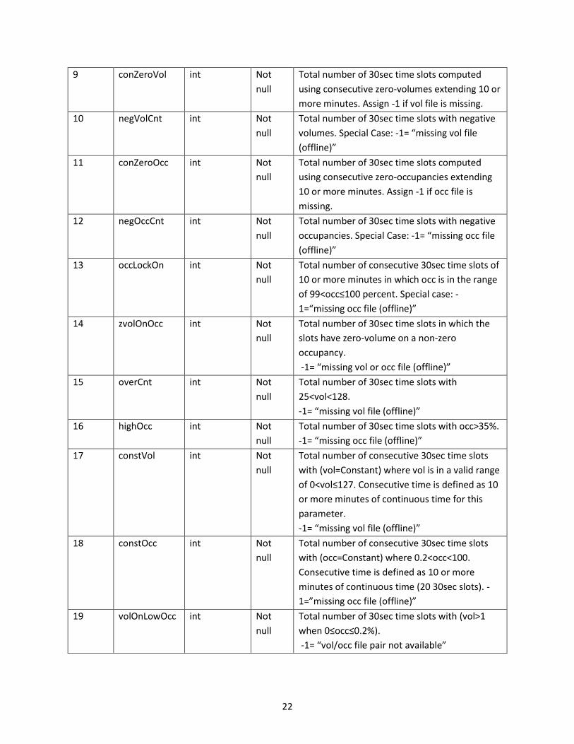
9 conZeroVol int Not
null
Total number of 30sec time slots computed
using consecutive zero-volumes extending 10 or
more minutes. Assign -1 if vol file is missing.
10 negVolCnt int Not
null
Total number of 30sec time slots with negative
volumes. Special Case: -1= “missing vol file
(offline)”
11 conZeroOcc int Not
null
Total number of 30sec time slots computed
using consecutive zero-occupancies extending
10 or more minutes. Assign -1 if occ file is
missing.
12 negOccCnt int Not
null
Total number of 30sec time slots with negative
occupancies. Special Case: -1= “missing occ file
(offline)”
13 occLockOn int Not
null
Total number of consecutive 30sec time slots of
10 or more minutes in which occ is in the range
of 99<occ≤100 percent. Special case: -
1=“missing occ file (offline)”
14 zvolOnOcc int Not
null
Total number of 30sec time slots in which the
slots have zero-volume on a non-zero
occupancy.
-1= “missing vol or occ file (offline)”
15 overCnt int Not
null
Total number of 30sec time slots with
25<vol<128.
-1= “missing vol file (offline)”
16 highOcc int Not
null
Total number of 30sec time slots with occ>35%.
-1= “missing occ file (offline)”
17 constVol int Not
null
Total number of consecutive 30sec time slots
with (vol=Constant) where vol is in a valid range
of 0<vol≤127. Consecutive time is defined as 10
or more minutes of continuous time for this
parameter.
-1= “missing vol file (offline)”
18 constOcc int Not
null
Total number of consecutive 30sec time slots
with (occ=Constant) where 0.2<occ<100.
Consecutive time is defined as 10 or more
minutes of continuous time (20 30sec slots). -
1=”missing occ file (offline)”
19 volOnLowOcc int Not
null
Total number of 30sec time slots with (vol>1
when 0≤occ≤0.2%).
-1= “vol/occ file pair not available”

23
20 corrCoef float4 Not
null
Correlation Coefficient computed using 30sec
vol and occ pairs. Assign corrCoef=0, if the
denominator of the formula becomes zero.
Assign corrCoef= -10 if vol/occ file pair not
available.
21 volOccRatio int Not
null
Total number of 30sec time slots violating the
acceptable range of vol/occ ratio.
-1= “vol/occ file pair not available”
22 detVol int Not
null
Total detector-volume of the day. Exclude
negative 30sec volumes (i.e., vol>127) in the
total.
-1= “missing vol file (offline)”
23 COV_ap varchar(2) null COV application status. N= not applied or
applicable, S=health level stayed same, U=
health-level upgrade, D=health-level
downgrade.
24 healthLevel varchar(1) null H=Healthy, T=Tolerable, I=Impaired,
N=Nonfunctional, O=Offline, G=Green counter
The second table the detectorhealth database is the COV_data table. This table stores the
computational results of COV applied to r_nodes.

24
Table 3: Column description of “cov_data” Table in detectorhealth Database
Column
Index
Column Heading Data
Type
Null Notes
0 cov_date date, primary key Not null format “yyyy-MM-dd”
1 r_node varchar(20),
primary key
Not null r_node name
2 staID varchar(15) null Station name
3 route varchar(20) null route name, ex: “I-694”
4 dir varchar(10) null route direction, ex: “WB”
5 cur_sta_vol int null current station volume from
selected detectors
6 cur_sta_conzero int null conZeroVol added from the main
station detectors
7 cur_sta_negcnt int null negVolCnt added from the main
station detectors
8 cur_offline int null number of off-line detectors at
the current station
9 cur_dets_selected varchar(80) null list of detectors selected for
curr_sta
10 up_sta_vol int null upstream station volume
11 up_sta_conzero int null conZeroVol added from the
upstream detectors
12 up_sta_negcnt int null negVolCnt added from the
upstream station detectors
13 up_offline int null number of off-line detectors at
the upstream station
14 up_dets_selected varchar(80) null list of detectors selected for
up_sta
15 dn_sta_vol int null downstream station volume
16 dn_sta_conzero int null conZeroVol added from the
downstream detectors
17 dn_sta_negcnt int null negVolCnt added from the
downstream station detectors
18 dn_offline int null number of off-line detectors at
the downstream station
19 dn_dets_selected varchar(80) null list of detectors selected for
dn_sta

25
20 lat float8 (string) null current r_node latitude
21 lon float8 (string) null current r_node longitude
Note:
9. The cur_dets_selected field follows the format of detector names separated by “/”.
14. 19. The up_dets_selected and dn_dets_selected fields follow the detector list format used in the Table-4,
COV_def table, columns 7 and 9.
3.3 DATA PROCESSING STEPS OF THE SERVER MANAGEMENT SOFTWARE
(DETHEALTH_DAILY)
The server includes a MySQL database engine and a sever management program called detHealth_daily.
This program is responsible for computing all detector-health parameters and then loading them to the
detectorhealth database. This section describes how the raw detector data are internally processed by
the server software, and then how the produced data are stored into the database. The details on user
level description of this software are available from the user manual, “detHealth_daily: User Manual,”
which is available from the software download web page.
The detHealth_daily program is designed to run daily by a Windows scheduler. The server software is
complex, and this section will attempt to describe the whole process by breaking them down to each
process in subsections.
3.3.1 Step1: Download metro_config.xml
The first process of detHealth_daily is to download information related to all currently- available traffic
detectors managed by RTMC. RTMC publishes most recent traffic detector information in their web site
in a form of compressed file with filename, metro_config.xml.gz. This file is a well-structured xml file
compressed using a gzip utility, which is a utility commonly available in UNIX or Linux operating systems
(OS’s). The record on when the content of this file changed is not available, and thus the history of new
detector allocations or removal can only be kept track of by downloading and archiving the gzip file
daily. Therefore, the first few steps are: download a metro_config.xml.gz file from the RTMC IRIS server,
uncompress it, add a timestamp in the file, and save to a storage. The filename is given a format of
metro_config.yyyymmdd.xml
where yyyy is a four-digit year, mm is a two-digit month, and dd is a two digit day. The folder for storing
this file can be set by user using the “Settings/Parameters” menu, but it is typically saved in the folder
with name “~/traffic/defines/metro_config/” in a file system. If a NAS is available, it should be stored in
a NAS since it is a critical file.

26
Each metro_config.xml file contains an xml data tree with hierarchically structured. At the top, the
whole roadway network is defined by a set of corridors, and then each corridor is defined by a road
name such as ‘I-35E’ and a direction attribute such as ‘SB’. Consequently, each corridor represents only
one direction of the road. The basic structure is described using an example, I-35E. The highway, I-35E,
consists of two corridors, ‘I-35E SB’ and ‘I-35E NB’. Each corridor is then defined using a set of r_nodes
that represent the following types at a location on the corridor.
“Station” (default and means Main),
“Exit”
“Entrance”
“Intersection”
“Access”
“Interchange”
One of the useful attributes of r_node in developing application is the GPS location information,
expressed in longitude and latitude. It can be used to pinpoint in a map where the r_node is and the
detectors belong to that location. Each r_node is next defined through nested elements. The following
xml shows an r_node defined for an entrance ramp in I-35E SB.
<r_node name='rnd_94495' n_type='Entrance' pickable='t' transition='Leg' label='Co Rd 14' lon='-
93.03155' lat='45.16164' lanes='1' shift='6' s_limit='70'>
<detector name='4973' label='35E/CR14SG' category='G'/>
<detector name='6412' label='35E/CR14SM' category='M' controller='ctl_95515'/>
<detector name='6445' label='35E/CR14SB' category='B' controller='ctl_95515'/>
<detector name='6446' label='35E/CR14SQ1' category='Q' lane='1' controller='ctl_95515'/>
<detector name='6447' label='35E/CR14SQ2' category='Q' lane='2' controller='ctl_95515'/>
<meter name='M35ES26' lon='-93.03196' lat='45.16266' storage='445'/>
</r_node>
Detector categories summarized in Table 4 can be seen here as a category attribute in the xml
statement. Detector category information is critical for the data processing and will be used in future
descriptions. Another important information used is the lane numbers, which was used in deriving
relationships of lanes for applying the COV principle.

27
Table 4: Detector Category
Category Description
A Auxilliary detector
B HOV bypass
G Count frame meter (number of greens)
M Merge detector of ramp
P Passage detector
Q Ramp queue meter
V Speed trap
X Exit Detector of ramp
D Shoulder
R Reversible
HT HOT lane
CD Collector/Distributor lanes (local-express
lanes)
H HOV lane
O Bus only lane
“” Blank, main lane default or not defined
3.3.2 Step2: Derive three equivalent detector sets for each r_node
After downloading a metro_config.xml file for the day, the program analyzes each corridor and r_nodes
in the corridor to determine equivalent detector sets. For each r_node with n_type=Station, equivalent
upstream and downstream station volume relations described in Section 2.3 and Figure 3 are derived
from the metro_config.xml file of the day. This result is saved as a CSV file with a timestamped filename
given by:
COV_def.yyyymmdd.csv
This file is saved in the folder “~/traffic/defines/COV_def/” and the timestamp matches with the
corresponding metro_config. yyyymmdd .xml file. The data processing is done by one corridor at a time,
and the following rules are applied in deriving a COV_def file.
Create a list of r_nodes in the order defined in the metro_config.xml file for the given route and
direction. Exclude r_nodes with active=’f’. Exclude all n_type=’Station’ with no detectors.
Include all n_type=’Entrance’ and ‘Exit’ even if they have no detectors. Exclude all r_nodes with
n_type = ‘Intersection’ or ‘Access’.

28
Pick three consecutive Station nodes. Label them upstream, current and downstream stations
following the lane traffic direction.
Derive r_node relations using Exit and Entrance nodes between consecutive Stations by
following the COV principle described using Eq. (5) and (6) in Section 2.3. Create a list of the
detectors corresponding to each r_node including signs determined by Eq. (5) and (6).
Table 5 describes each column of a COV_def CSV file. This table is constructed based on r_nodes, and
the columns 0 – 4 are used as the identity of the current r_node, which are def_date, r_node name,
station ID (staID), route, and direction (dir). To define upstream and downstream equivalent stations, a
list of r_nodes are provided using a separator “&” and “+” or “-“ sign, under the column headings of
up_rnodes and dn_rnodes. For an r_node description, sign prefix is required even for “+”. The following
shows an example.
+rnd_2345&-rnd_34449&+rnd_0899
This string instructs that volumes of r_nodes, rnd_2345 and rnd_0899, must be added, while the volume
of rnd_34449 must be subtracted to compute the total station volume. These r_node relations are
translated into a list of detectors and then stored in column names: cur_det_list, up_det_list, and
dn_det_list.
The data type of cur_det_list column is a text string, and it consists of detector names of the current
station separated by “/”. For example, if string of a current station was “2345/4567/2346”, the station
has detectors with names, “2345”, “4567”, and “2346”. All of them are expressed without sign and takes
positive sign by default, because the current node is always a station. If a lane has more than one
detector, all detectors must be listed, but it does not have to follow the order of lane numbers.
Detector lists stored in up_det_list, and dn_det_list columns use a more complex syntax. Since station
volumes are a function of r_nodes and its node types (n_type), it specifies n_type followed by a list of
detectors of that r_node. The final n_type prefixes used are S= “Station”, E= “Entrance”, and X= “Exit”
with all capital letters. Separator “&” divides r_nodes and “/” divides detectors. A plus sign (“+”)
indicates addition while a negative sign (“–”) indicates subtraction in computing the r_node volumes
from the total station volume, and the signs are only applied at the r_node level (i.e., not detector level).
An example string of an equivalent station with two entrance nodes and one exit node is given by:
+S2456/3457/3458/T5687&-E456/457/458/T5687&-E678/8974/345&+X2456/3457
The volume of this station is computed by:
Station_volume = vol(2456) + vol(3457) + vol (3458) + vol(T5687) - vol (456) - vol (457) – vol(458) –
vol(T5687) – vol(678)-vol(8974) – vol(345) + vol(2456) + vol(3457)
where vol(####) denotes a single day volume of detector name “####”.

29
Some Exit and Entrance nodes may not have any detectors, and thus a syntax with no detectors are
allowed. For example, “+S2435/345&-E&+X” is acceptable and indicates that the Entrance and Exit
r_nodes do not have any detectors. For this specification, all “G” detectors are excluded in the detector
list, since G detectors are not traffic detectors but counters used for storing a number of green light
counts occurred in a freeway Entrance ramp.
Table 5: COV Defines Table
Column
Index
Column
Heading
Data
Type
Null Notes
0 def_date date,
primary key
Not null the date of metro_config file used to
produce this file
1 r_node varchar(20),
primary key
Not null r_node name, only n_type=Station
2 staID varchar(10) null Station name. If staID=“”, leave it as
blank
3 route varchar(20),
primary key
not null route name, ex: I-694
4 dir varchar(10),
primary key
not null direction of the route
5 cur_det_list varchar(80) null list of all detector names defined in the
current station
6 up_rnodes varchar(80) null list of equivalent upstream r_nodes
7 up_det_list varchar(120) null detector list of equivalent upstream
station
8 dn_rnodes varchar(80) null list of equivalent downstream r_nodes
9 dn_det_list varchar(120) null detector list of equivalent downstream
station
10 lat float8 (string) null current r_node latitude
11 lon float8 (string) null current r_node longitude
3.3.3 Step 3: Compute all detector-health parameters
The parameters specified in the columns 9 -24 in Table 2 are computed using the raw volume and
occupancy data queried and received from the IRIS server. For this computation, threshold values of the
health-level classifier described in Figure 2 are first read in from a file. This table is user programmable
and saved in a CSV format given in Table 6. The file is stored in the
“~/traffic/defines/health_thresholds/” folder and has a timestamp in the middle of the filename; the file
name takes the following format:
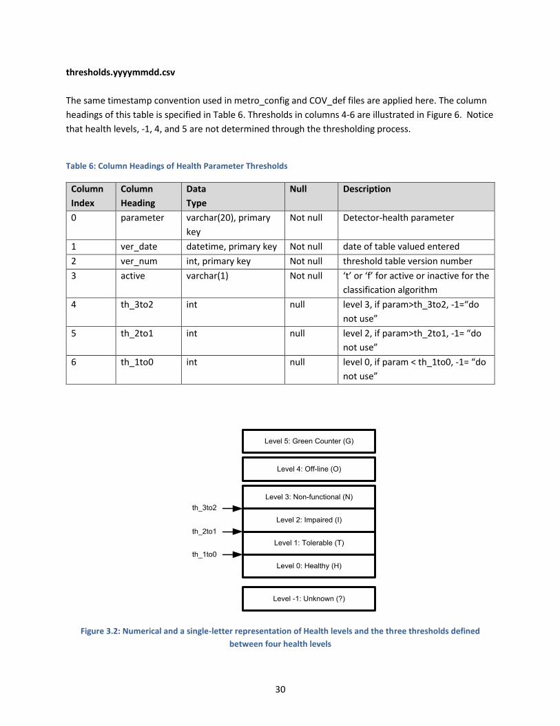
30
thresholds.yyyymmdd.csv
The same timestamp convention used in metro_config and COV_def files are applied here. The column
headings of this table is specified in Table 6. Thresholds in columns 4-6 are illustrated in Figure 6. Notice
that health levels, -1, 4, and 5 are not determined through the thresholding process.
Table 6: Column Headings of Health Parameter Thresholds
Column
Index
Column
Heading
Data
Type
Null Description
0 parameter varchar(20), primary
key
Not null Detector-health parameter
1 ver_date datetime, primary key Not null date of table valued entered
2 ver_num int, primary key Not null threshold table version number
3 active varchar(1) Not null ‘t’ or ‘f’ for active or inactive for the
classification algorithm
4 th_3to2 int null level 3, if param>th_3to2, -1=“do
not use”
5 th_2to1 int null level 2, if param>th_2to1, -1= “do
not use”
6 th_1to0 int null level 0, if param < th_1to0, -1= “do
not use”
Figure 3.2: Numerical and a single-letter representation of Health levels and the three thresholds defined
between four health levels
Level 0: Healthy (H)
Level 3: Non-functional (N)
Level 2: Impaired (I)
Level 1: Tolerable (T)
Level 4: Off-line (O)
th_1to0
th_2to1
th_3to2
Level 5: Green Counter (G)
Level -1: Unknown (?)

31
Figure 3.3: Settings window available in detHealth_daily for programming threshold levels
Threshold levels are designed to be programmable by user using the settings window shown in Figure 7.
It should be noted that entry “-1” means that the corresponding threshold is not used. Below describes
the actual implementation of the thresholding processes in the health level (HL) classification applied in
detHealth_daily.exe. A general rule is given first and then then details of each case is described.
Test is performed starting from HL=4 and then moved down to the next lower level. The cases
survived the last test become HL=0 (healthy).
All if-conditions per given HL are in OR relationship, i.e., if any of the listed conditions is met, it
selects the assigned HL.

32
HL =5 (G), if
Detector category (det_cat) = G, special case, not programmable
else continue
HL =4 (O), if
negVolCnt=-1, special case, not programmable
else continue
HL =3 (N), if
1. zVolOnOcc=2880, special case, not programmable
2. conZeroVol=2880 for five or more days (not implemented yet)
else continue
HL =3 (N), if
1. negVolCnt > 2736 (95%), negVolCnt.th_3to2=2736
2. negOccCnt > 2736 (95%), negOccCnt.th_3to2=2736
3. occLockOn: not used, occLockOn.th_3to2= -1
4. zVolOnOcc: not used, zVolOnOcc.th_3to2= -1
5. overCnt > 2736 (95%), overCnt.th_3to2=2736
6. highOcc: not used, highOcc.th_3to2= -1
7. constVol >240 (2hr), constVol.th_3to2=240
8. constOcc > 240 (2hr), constOcc.th_3to2=240
9. volOnLowOcc: not used, volOnLowOcc.th_3to2= -1
10. volOccRatio: not used, volOccRatio.th_3to2= -1
11. conZeroVol: not used, conZeroVol.th_3to2= -1
12. conZeroOcc: not used, conZeroOcc.th_3to2= -1
13. COV_th: not used, COV_th.th_3to2= -1
else continue
HL = 2 (I), if
1. (conZeroVol + negVolCnt)=2800 and negVolCnt>5, not programmable
2. negVolCnt > 1440 (50%), negVolCnt.th_2to1=1440
3. negOccCnt: not used, negOccCnt.th_2to1= -1
4. occLockOn > 2304 (80%), occLockOn.th_2to1=2304
5. zVolOnOcc > 2304 (80%), zVolOnOcc.th_2to1=2304
6. overCnt > 2304 (80%), overCnt.th_2to1=2304
7. highOcc > 2592 (90%), highOcc.th_2to1=2592
8. constVol : not used, constVol.th_2to1= -1
9. constOcc : not used, constOcc.th_2to1= -1
10. volOnLowOcc: not used, volOnLowOcc. th_2to1= -1
11. volOccRatio> 2304 (80%), volOccRatio.th_2to1=2304
12. conZeroVol>2870 (99%), conZeroVol.th_2to1 = 2870
13. conZeroOcc: not used, conZeroOcc.th_2to1 = -1
14. COV_th: not used, COV_th.th_2to1= -1

33
else continue
HL = 1 (T), if
1. negVolCnt > 120 (1hr), negVolCnt.th_1to0=120
2. negOccCnt: not used, negOccCnt.th_1to0= -1
3. occLockOn > 120 (1hr), occLockOn.th_1to0=120
4. zVolOnOcc > 1152 (40%), zVolOnOcc.th_1to0=1152
5. overCnt > 120 (1hr), overCnt.th_1to0=120
6. highOcc: not used, highOcc. th_1to0= -1
7. constVol > 120 (1 hr), constVol.th_1to0=120
8. constOcc > 120 (1 hr), constOcc.th_1to0=120
9. volOnLowOcc > 120 (1 hr), volOnLowOcc.th_1to0=120
10. volOccRatio: not used, volOccRatio.th_1to0= -1
11. conZeroVol: not used, conZeroVol.th_1to0 = -1
12. conZeroOcc: not used, conZeroOcc.th_1to0 = -1
13. COV_th>30%, COV_th.th_1to0= 30 (algorithm includes more conditions)
else
HL = 0 (H), remaining cases.
The final output file is created as a CSV formatted file that exactly matches with the columns defined in
Table 2. The file name follows the same timestamp convention with the “health_param” prefix, which is
shown below.
health_param.yyyymmdd.csv
This file is save in the default folder, “~/traffic/processed/det_health_param/”, or in a user defined
folder.
3.3.4 Step 4: Apply COV rule-checks for applicable r_nodes
After computation of all parameters as described in Section 3.3.3, HL is first adjusted based on COV
relations within a single r_node. The first character of COV_ap parameter represents the result of this
step. There are two cases, when n_type=’Station’ and more than one detectors per lane exist, and when
n_type= ‘Entrance’. The rules for using spatial relations are described below.
(1) n_type=’Station’
A. If a lane has only a single detector, do nothing
B. If a lane has more than one detector (commonly two):
Let the two detector volumes be denoted x and y.
(i) if x=-1 or y=-1, do nothing
(ii) if x=y=0 and negVolCnt<negVolCnt.th_1to0, assign HL=“T”
(iii) if x=0 and y<>0, assign HL=“I”

34
Otherwise, compute the difference ratio,
𝛼 =|𝑦−𝑥|
(𝑥+𝑦)/2
(iv) if α<0.2, assign both HL=“H”
(v) if 0.2≤ α<0.35, assign HL=“T”, else HL=”I”
(vi) assign the value of COV_ap according to the HL change made (U, D, or S depending on the
change by this process)
(2) n_type = ‘Entrance’
(i) If det_cat = “B” or “O” and negVolCnt < negVolCnt.th_1to0, then HL=”H”.
(ii) If HL of all detectors consist of only “H” and “O”, do not change and exit.
(iii) Spatial relation test. (For volume totals, do not add detVol=-1)
-- Add volumes of all P’s and B’s, and call PB_vol
--Add volumes of all Q’s and call Q_vol
--Add volumes of all M’s and call M_vol
Check if PB_vol≈ Q_vol≈ M_vol and negVolCnt< negVolCnt.th_1to0, then upgrade the corresponding
detectors to HL=“H”. A similarity requirement is satisfied when the differences are less than 10%
(default value).
(3) n_type = ‘Exit’
If det_cat = “O” and negVolCnt < negVolCnt.th_1to0, then assign HL=”H” else no change.
3.3.5 Step 5: Adjust HL according to COV tests for r_nodes with main -lane stations
In Step 4, COV was used within a single r_node when redundant detectors with equivalent traffic flows
are available. In Step 5, the COV principle is applied in three equivalent traffic-flow stations in main
lanes. The equivalent stations consist of three stations: current station, equivalent upstream station,
and equivalent downstream station. How to add or subtract certain detector volumes to maintain the
equivalency between the three stations was described in Section 2.4, and the actual detector volume
relations among associated detectors are defined in the “COV_def.yyyymmdd.csv” file that matches the
date. The computed data according to a “COV_def.yyyymmdd.csv” file is saved in a COV_data.csv file
with the same timestamp included in the COV_def filename, i.e.,
COV_data.yyyymmdd.csv
This file is archived in the “~/traffic/processed/COV_data/” folder and later loaded to the database table
cov_data.
To test if the stations met the requirement of COV rule or not, another intermediate data file is
produced. Let three consecutive equivalent station volumes be denoted: up_vol, cur_vol, and dn_vol.
For similarity measurements, normalized difference ratios are computed following the steps below.

35
Two volumes are considered similar if the difference ratio is less than 0.05 when the difference
ratio between v1 and v2 is computed as:
𝑑𝑖𝑓𝑓_𝑟𝑎𝑡𝑖𝑜(𝑣1, 𝑣2) = |𝑣1 − 𝑣2|/(𝑣1+𝑣2
2)
Compute diff_ratio(up_vol, cur_vol) and diff_ratio(cur_vol, dn_vol)
Detectors are considered healthy if the resulting diff_ratio is less than 0.05, and they are listed under
the column heading good_dets. For example, if diff_ratio(up_vol, cur_vol) is less than 0.05, all detectors
involved in the current and upstream stations are considered to be candidates for HL upgrade. To save
diff_ratio data, a CSV file is created with its data formatted with the columns defined in Table 7. Its
filename starts with “COV_diffRatio” followed by a timestamp of the date, i.e.,
COV_diffRatio.yyyymmdd.csv
This file is stored in the “~/traffic/processed/COV_data/” folder. The detectors listed under the column
heading, good_dets, satisfy the COV rule and are the detectors to be upgraded to HL=H.
Table 7: Column Headings and Data Types of COV_diffRatio.csv Table
Column
Index
Column
Heading
Data
Type
Null Notes
0 route varchar(20),
primary key
not null route name, ex: I-694
1 dir varchar(10),
primary key
not null direction of the route
2 r_node varchar(10),
primary key
not null r_node representing current node
3 up_cur_ratio float4 null Difference of ratio between upstream
and current station volumes. Format
(“F5”)
4 cur_dn_ratio float4 null Difference of ratio between downstream
and current station volumes. Format
(“F5”)
5 good_dets varchar(120) null a list of detectors that are found to be
HL=”H” according to the COV test.

36
In order to keep track of which detectors are upgraded following the main lane COV rules, the detectors
upgraded are listed in COV_upgradeDets.yyyymmdd.csv in which each line is the state before upgrade.
An example of this file is shown in Figure 8, which is the content of the file for May 30, 2019. Again, it
contains the record of each detector before upgraded to H.
Figure 3.4: COV_upgradeDets.20190530.csv
det_date,route,dir,staID,r_node,detID,lane,det_cat,abandoned,conZeroVol,negVolCnt,conZeroOcc,negOccCnt,occLockOn,zvolOnOcc,Over
Cnt,highOcc,constVol,constOcc,volOnLowOcc,corrCoef,volOccRatio,detVol,COV_ap,healthLevel
2019-05-30,I-35E,NB,Exit,rnd_87679,3377,0,X,f,2880,0,2880,0,0,0,0,0,0,0,0,0.000000,0,0,N,I
2019-05-30,I-35W,NB,S1702,rnd_168,6911,1,,f,0,1165,0,1165,0,3,0,0,0,0,0,0.972324,1171,16175,N,T
2019-05-30,I-35W,NB,S1702,rnd_168,6912,2,,f,0,1165,0,1165,0,0,0,0,0,0,0,0.965952,1172,15095,N,T
2019-05-30,I-35W,NB,S1702,rnd_168,6913,3,HT,f,0,1165,0,1165,0,0,0,0,0,0,0,0.972900,1171,11335,N,T
2019-05-30,I-35W,NB,S38,rnd_86379,271,1,,f,0,1160,0,1160,0,0,0,0,0,0,0,0.975868,1166,16216,N,T
2019-05-30,I-35W,NB,S38,rnd_86379,272,2,,f,0,1160,0,1160,0,0,0,0,0,0,0,0.964144,1166,15103,N,T
2019-05-30,I-35W,NB,S38,rnd_86379,541,3,HT,f,0,1160,0,1160,0,2,0,0,0,0,0,0.989233,1170,9590,N,T
2019-05-30,I-35W,NB,S40,rnd_86391,275,1,,f,0,0,0,0,0,0,0,39,0,0,0,0.765087,49,23886,D,I
2019-05-30,I-35W,NB,S55,rnd_95787,5963,1,,f,2876,0,2876,0,0,0,0,0,0,0,0,0.827297,1,4,N,I
2019-05-30,I-35W,NB,S58,rnd_86483,322,4,,f,2880,0,2880,0,0,0,0,0,0,0,0,0.000000,0,0,N,I
2019-05-30,I-35W,NB,S58,rnd_86483,6792,5,HT,f,2880,0,2880,0,0,0,0,0,0,0,0,0.000000,0,0,N,I
2019-05-30,I-35W,NB,ST519,rnd_5771,T3521,1,HT,f,0,818,1683,818,0,0,6,0,0,0,1855,0.000000,818,16691,N,T
2019-05-30,I-35W,NB,S62,rnd_86499,T3506,1,,f,0,1572,0,1572,0,0,0,0,0,0,1072,0.000000,1572,16946,S,I
2019-05-30,I-35W,NB,S664,rnd_87489,2734,3,,f,2880,0,2880,0,0,0,0,0,0,0,0,0.000000,0,0,N,I
2019-05-30,I-35W,SB,S678,rnd_87787,2785,1,,f,2880,0,2880,0,0,0,0,0,0,0,0,0.000000,0,0,N,I
2019-05-30,I-35W,SB,S29,rnd_88039,252,1,,f,0,1160,0,1160,0,0,0,2,0,0,0,0.939849,1168,15115,N,T
2019-05-30,I-35W,SB,S29,rnd_88039,253,2,,f,0,1160,0,1160,0,0,0,8,0,0,0,0.927724,1165,18723,N,T
2019-05-30,I-35W,SB,S29,rnd_88039,1001,3,HT,f,0,1160,0,1160,0,0,0,0,0,0,0,0.980668,1168,11488,N,T
2019-05-30,I-35W,SB,S1715,rnd_177,6908,1,,f,0,1167,0,1167,0,0,0,3,0,0,0,0.935885,1172,15291,N,T
2019-05-30,I-35W,SB,S1715,rnd_177,6909,2,,f,0,1167,0,1167,0,1,0,12,0,0,0,0.931156,1169,18875,N,T
2019-05-30,I-35W,SB,S1715,rnd_177,6910,3,HT,f,0,1167,0,1167,0,2,0,0,0,0,0,0.978746,1168,12036,N,T
2019-05-30,I-394,EB,S284,rnd_88327,793,1,,f,0,0,0,8,0,0,0,255,0,0,0,0.452633,36,23199,D,T
2019-05-30,I-694,WB,S178,rnd_87149,16,3,,f,2880,0,2880,0,0,0,0,0,0,0,0,0.000000,0,0,N,I
2019-05-30,I-694,WB,S176,rnd_87153,762,3,,f,2880,0,2880,0,0,0,0,0,0,0,0,0.000000,0,0,N,I
2019-05-30,T.H.36,WB,S589,rnd_86737,2304,2,,f,2880,0,2880,0,0,0,0,0,0,0,0,0.000000,0,0,N,I
2019-05-30,T.H.36,WB,S612,rnd_86739,2336,2,,f,2880,0,2880,0,0,0,0,0,0,0,0,0.000000,0,0,N,I
2019-05-30,T.H.52,SB,Exit,rnd_89735,5554,0,X,f,2880,0,2880,0,0,0,0,0,0,0,0,0.000000,0,0,N,I
2019-05-30,T.H.61,NB,Exit,rnd_1586,7497,0,X,f,234,166,234,166,0,11,0,0,0,0,0,0.945813,195,2018,N,T
2019-05-30,T.H.61,NB,S1931,rnd_1585,7453,1,,f,0,166,0,166,0,3,0,0,0,0,0,0.944255,187,14650,N,T
2019-05-30,T.H.61,NB,S1931,rnd_1585,7454,2,,f,0,166,0,166,0,7,0,0,0,0,0,0.981343,170,10987,N,T
2019-05-30,T.H.61,SB,S1896,rnd_1266,7378,1,,f,0,166,0,166,0,6,0,0,0,0,0,0.951461,187,14662,N,T
2019-05-30,T.H.61,SB,S1896,rnd_1266,7379,2,,f,27,166,27,166,0,4,0,0,0,0,0,0.986732,170,11709,N,T
2019-05-30,T.H.61,SB,Entrance,rnd_1573,7487,0,M,f,303,166,303,166,0,11,0,0,0,0,0,0.940157,229,2004,N,T
To illustrate the HL changes, the final detector records in the file health_param.20190530.csv are shown
in Figure 9 (only for the first four detector records in Figure 8). Notice that health levels are upgraded to
H from I or T. It can be also seen that COV_ap column is set to “NU” in which “N” indicates that HL was
not modified from the single r_node COV algorithm but “U” indicates that HL was upgraded after
application of the COV rule on the main-lane stations.

37
Figure 3.5: Health level upgrades applied in health_param.20190530.csv for the first four detectors in Figure 3.4.
3.3.6 Step 6: Upload health_param and COV_data to the MySQL detectorhealth
database
The final computed records in CSV files (health_param.yyyymmdd.csv and COV_data. yyyymmdd.csv) for
the day of computation are one-to-one matches with the corresponding database entries, and they are
directly loaded to the detectorhealth database, using two steps: (1) if old data exists for the same day,
delete it first, (2) load the latest data computed. These two steps ensure that only the most-recently
computed data are loaded to the database.
For loading data to MySQL tables, loading each row at a time is not efficient and time consuming. A
more efficient way is used. The solution is use of an import function in MySQL, and it directly loads the
CSV file in bulk to the corresponding table. Only restriction of this approach is that it voids if duplicate
records are found, determine by primary keys. This problem is resolved, if the old data are removed
before importing. This operation is robust and runs much faster than individual loading of records.
Below shows an example of MySQL script used for importing one-day data, which was health_param for
Nov 15, 2018. A similar script was used for COV_data.
Figure 3.6: MySQL script for importing one day of health_param data file
use detectorhealth;
load data local infile 'Y:\\traffic\\processed\\det_health_param\\2018\\health_param.20181115.csv'
into table health_param
fields terminated by ','
lines terminated by '\r\n'
ignore 1 lines;
det_date,route,dir,staID,r_node,detID,lane,det_cat,abandoned,conZeroVol,negVolCnt,conZeroOcc,negOccCnt,occLockOn,zvolOnOcc,Over
Cnt,highOcc,constVol,constOcc,volOnLowOcc,corrCoef,volOccRatio,detVol,COV_ap,healthLevel
2019-05-30,I-35E,NB,Exit,rnd_87679,3377,0,X,f,2880,0,2880,0,0,0,0,0,0,0,0,0.000000,0,0,NU,H
2019-05-30,I-35W,NB,S1702,rnd_168,6911,1,,f,0,1165,0,1165,0,3,0,0,0,0,0,0.972324,1171,16175,NU,H
2019-05-30,I-35W,NB,S1702,rnd_168,6912,2,,f,0,1165,0,1165,0,0,0,0,0,0,0,0.965952,1172,15095,NU,H
2019-05-30,I-35W,NB,S1702,rnd_168,6913,3,HT,f,0,1165,0,1165,0,0,0,0,0,0,0,0.972900,1171,11335,NU,H

38
A total run time for a single day computation and uploading to the database took about 4 minutes of
processing time on a PC with i7 CPU that runs on 3.6 GHz clock and 16GB RAM. This processing time is
highly dependent on Internet traffic and speed but it took less than 5 minutes in most cases.
3.4 FUNCTIONS OF SERVER MANAGEMENT SOFTWARE
Manual management of the detector-health database would be time consuming and tedious. In order to
simplify the sever management operations, a utility program, detHealth_daily.exe, was developed to
automatically control all data processing steps and management of the MySQL database in the server,
i.e., all steps are automated and it runs once daily through a Windows scheduler. This section briefly
describes the features of this software and utilities. The details on how to use this program is available
on-line through a user manual.
Figure 11 shows the GUI of detHealth_daily.exe that is used for illustration. This tool can be used for two
types of runs, manual and scheduled. For manual runs, user selects a date from the DateTimePicker
provided and presses the “One Day Manual Run” button. This will compute all required parameters for
the selected date and then load them to the database. The “Auto Run” button processes (computes and
upload daily data to database) data for one day at a time from the last ending date set in the Settings to
the most recent day (yesterday). This function is called by the Windows Scheduler when daily
scheduled-runs are triggered. When it is manually used, this function allows the process to fill in the
database to the most recent date. For example, suppose that the RTMC IRIS server or the database
server failed for several days. Then, the database must be populated from the date of failure to the most
recent day, and a single press of the “Auto Run” button will do the job for populating the missing data.
There is also a need for creating or restoring data for a specific period defined by user. Suppose that the
database was failed for some reason for a specified period. In such a case, the user should be able to run
and restore data for a specific period. Another case would be to create past data for a period where
data was never created. For these cases, a manual run function for a period defined by Start and End
dates is used, and it can be executed using the interface shown below.
The “Run All in One Click(...)” button function goes through five steps for producing and storing health-
parameters: (1) compute health-parameters, (2) compute COV_def file, (3) compute COV_data and
adjust HL, (4) upload health-parameters to database, and (5) upload COV_data to database. These
individual steps can be run for the given period, one-step at a time using the individual buttons provided

39
in the lower half of the groupbox labeled “Manual Runs from Start-to-End Dates.” It should be cautioned
that Steps 1-3 must run by following the numerical order provided, i.e., (1), (2), and (3). One scenario
that these partial steps could be useful is when the database failed but detHealth_daily ran, resulting
successful production of all health parameters. In this case, steps (4) and (5) could be used to restore the
data.
The second tab (named Test Functions) provides several utilities, mostly for manually testing of the
database. It includes a test function for downloading the most recent metro_config file and six buttons
for database content tests. These tests are all designed to inquire and test a single day data specified in
the date textbox. The first four buttons are to get answers or to take an action related to health_param
in the database. This should be mainly used by a database administrator to check if the processing was
run for a certain date and then to take actions. Here are four tests corresponding to the four buttons.
“Do health-parameters for the given date exist in the database?” This button is used to check if
the data for the Date textbox exists in the database.
“Upload the health-parameter data (in the form of CSV) available for the given date to
database.” This button uploads the health_param.yyyymmdd.csv data in the detector-health
parameter folder to the database, corresponding to the Date textbox.
“Delete the health-parameters from the database for the given date.” This button deletes all
detector-health parameters specified in the Date textbox.
“If data exist in DB for the given date, delete them first then upload.” This button deletes the
health-parameters that already exist in the database for the date given in the Date textbox and
then loads fresh new data for the same date from the detector-health parameter folder.
Existence test and delete functions exist for the COV database. The two buttons available are:
“Does COV_data exist in DB for the given date?”
“Delete the given date of COV_data in the database.” This button checks existence of COV_data
for the date in the Date textbox, and then deletes them if they exist.
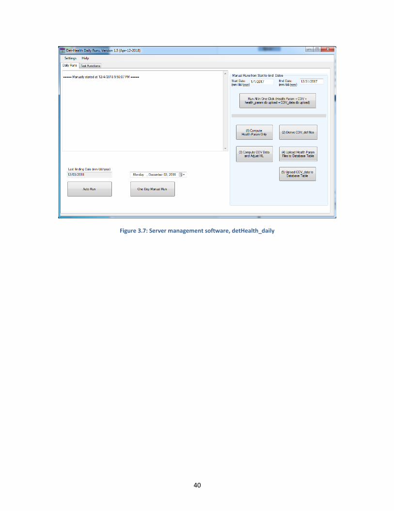
40
Figure 3.7: Server management software, detHealth_daily

41
3.5 CLIENT SOFTWARE: DETHEALTH_APP
A client software tool, called “detHealth_app,” was created to provide a data tool that utilizes the
detector-health database. This utility was designed as an exploration tool for detector and station level
data for up to one year from the ending date entered by user. It also provides utilities with map
interfaces to give spatial information of detectors and stations. Since a separate user manual entitled
“detHealth_app: User Manual” is available on line, only the key features of the software are described.
detHealth_app currently consists of four tabs and its screen capture is shown in Figure 12. Functions
available in each Tab are described based on the Version 2.1 (May 17, 2019). This software continuously
evolves as the MnDOT needs change over time, and future versions will likely be different from the one
described here.
Figure 3.8: First tab of detHealth_app

42
Tab 1: Detectors. This tab provides a pie chart and listboxes of detector classification for the date
selected by the DateTimePicker tool. Five listboxes are provided for five classes: Healthy, Tolerable,
Impaired, Nonfunctional, and Off-line. Pressing any of the detectors in the list immediately displays all
detector-health parameters of the day in the Selected Detector textbox. The first tab also includes a
utility for retrieving historical data. This utility is controlled using the selection tools in the groupbox
labeled “Historic Data of the Selected Detectors” and multiple detectors can be listed with comma
separation in the Detector List textbox. The ending date should be selected using the provided date-time
picker. Historic data is then retrieved with three options: last one month, last six months, or last one
year from the user selected ending date. The retrieved data from database can be viewed using a graph
or an Excel spreadsheet. If one year past data is selected, AADT computed using the AASHTO method
(AASHTO Guidelines for Traffic Data Programs, 2009) is displayed in the graph.
Tab 2: Stations. This tab provides data for a collection of stations that satisfy the COV principle. The data
can be loaded for the date specified in the date-time picker tool. Once it is loaded, a station (main-lane
r_node) can be selected by a mouse click from the map provided or from the listbox, which would then
produce all related information in a callout box as well as in a textbox. The precise location of the station
can also be plotted in a Google map. Historic data of the selected station could be retrieved for one
month, six months, or one year, and then outputted in a graph or a spreadsheet. One year data retrieval
provides an AADT computed using the AASHTO method.
Tab 3: r_node Map. The third tab provides navigation of r_nodes and detectors in the RTMC
metro_config file through a map. RTMC defines a location on a road using an r_node for all roads. Types
of r_nodes include Station, Exit, Entrance, Intersection, Access, and Interchange, and each of the
location is specified using GPS coordinates. If an r_node is a station, it represents a set of detectors on a
road covering all main lanes at that specific location. Exit and Entrance r_nodes are similarly defined,
and all detectors in the Exit or Entrance ramps become members of the r_node. Intersections and
interchanges are transitional r_nodes of roads. Many r_nodes do not have detectors, and it is assigned
for future locations of detectors or for identification of a specific location on the road. One of the useful
tools in this tab is a search function of an r_node or a detector. After entering a detector or an r_node ID
in the respective textbox and then clicking the search button points to the corresponding corridor and
r_node, along with all detector information. The information includes corridor, station ID, node type,
active or not, address, latitude/longitude, and detectors with lane numbers. It also provides a function
to plot the r_node in a Google map. One month worth of volumes for any selected r_node is retrieved
and plotted using the “Plot last one month of the r_Node” button.

43
Tab 4: Data Direct. This tab provides retrieval utilities for volume and detector-health parameters up to
one year without using the detector-health database. One of the data types not available from the
detector-health database is hourly volumes. This tab provides hourly volumes for one day, 10 days, one
month, or six months. It also provides retrieval functions for length-based vehicle classification. Retrieval
types can be selected in intervals of hourly or daily. Since the functions implemented in this tab do not
use the detector-health database, this tool provides access to detector-health data when the database is
not reachable or not available.

44
CHAPTER 4: DATA ANALYSES
This chapter describes some of data studies completed in “Task 2: Evaluation of Detector-Health
Algorithm on a Corridor Study” and few selected examples on the use of the detHealth_app software
tool.
4.1 HISTOGRAM ANALYSIS
Histograms provide information on underlying distribution of the given sample data, and it is commonly
used as a first step to look into the characteristics of the data. In this project, histogram analyses were
used as part of Task 2: Corridor Study, in which I-694 and I-94 data on 2015 and 2016 were used. The
analysis results were reported in the Task 2 report.
This section shows histograms of 2018 data on I-694 (EB and WB). Distribution patterns were very
similar to that of 2015 and 2016. Histogram data were computed using all detectors in I-694 EB and WB,
except for two types of detectors. The first type of detectors excluded were those detectors that are
labeled true in the “abandoned” attribute. Another type of detectors excluded were those detectors
that had “G” in its category name, because they are not actually detectors but green light counters in
highway entrance ramps. The total number of records in 2019 excluding the detectors mentioned above
for I-694 was 139,197.
In all histogram data presented here, bins were created based on the number of 30-second time slots
allocated by increments of one hour, producing 24 bins. Since one hour contains 120, 30-second time
slots, the range was incremented by 120. The label of each bin is expressed using two numbers
separated by a two-character symbol “->”. For example, “120->239” indicates that the range of this bin
is [120,239] or 120 ≤ 𝑥 ≤ 239, and the number in the bin indicates occurrences of detector-health
parameters. For example, consider ConZeroVol, which is a count of consecutive zero volumes in 30-
second time slots. If ConZeroVol of this detector on a day is 180, it means that consecutive zero volumes
were observed for one and half hours and the bin [120, 239] is incremented by one. Because there were
a large number of cases that fall at 0, i.e., zero occurrence of the parameter for the whole day, this case
was assigned to a separate bin labeled “0-only.” Similarly, many cases also fall at 2880, i.e., occurrence
of the parameter for the whole day, and it deserves a separate bin. This bin is labeled “2880-only.” In
summary, all histograms contain twenty-six bins. The complete histogram data for all detector-health
parameters of I-694 in 2018 is attached in Appendix A. The histogram data also includes percentage of
each bin in a separate column.
In general, three distribution patterns were observed. The first type shows very high frequencies in bins
[0-only] and [1, 119] followed by an exponential drop but then frequency rises again in the last bins
[2760, 2879] and [2880-only]. This characteristic is shown in Figure 13, and the parameters showing this
pattern include ConZeroVol, NegVolCnt, zVolOnOcc and volOccRatio. It should be mentioned that the
histogram of ConZeroOcc was nearly identical to that of ConZeroVol and thus omitted.

45
Figure 4.1: Histograms of ConZeroVol, NegVolCnt, zVolOnOcc and volOccRatio parameters on I-694 2018 data
0
20000
40000
60000
80000
100000
120000
0-o
nly
1->
11
9
12
0->
23
9
24
0->
35
9
36
0->
47
9
48
0->
59
9
60
0->
71
9
72
0->
83
9
84
0->
95
9
96
0->
10
79
10
80
->1
19
9
12
00
->1
31
9
13
20
->1
43
9
14
40
->1
55
9
15
60
->1
67
9
16
80
->1
79
9
18
00
->1
91
9
19
20
->2
03
9
20
40
->2
15
9
21
60
->2
27
9
22
80
->2
39
9
24
00
->2
51
9
25
20
->2
63
9
26
40
->2
75
9
27
60
->2
87
9
28
80
-on
ly
Freq
uen
cy
Bin Range in Number of 30 Second Time Slots
ConZeroVol
NegVolCnt
zVolOnOcc
volOccRatio
The second distribution pattern observed was concentration of distribution in the [0-only] bin, which
indicates that these parameters rarely happen. The parameters in this category include OccLoackOn,
ConstVol, ConstOcc, and volOnLOwOcc. Since these parameters rarely happen, two interpretations may
be considered: (1) ignore these parameters in determining detector-health level or (2) consider that the
quality of the detector data on that day is low when one of these parameters is observed. In this test
data, non-zero OccLockOn (10 or more consecutive minutes in which occupancy is in between 99 and
100 percent) occurred only 11 times out of 130,067 detector days (number of detectors * 365), which is
very low and shows that this condition rarely occurred.
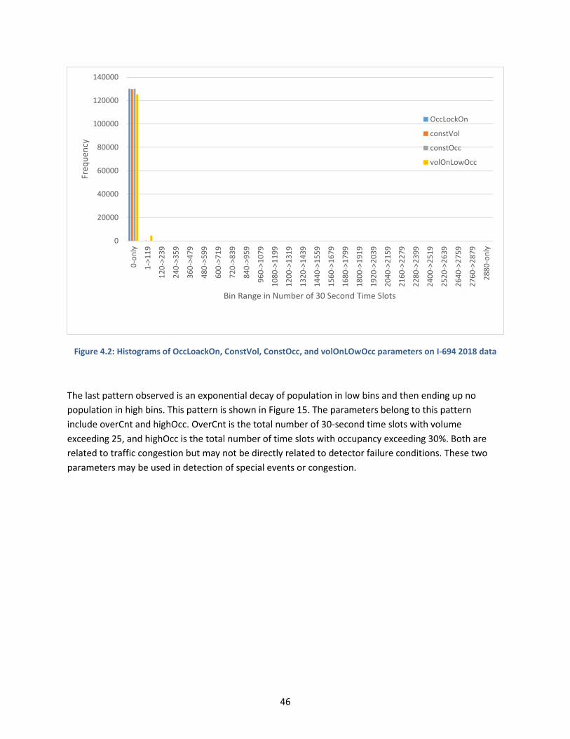
46
Figure 4.2: Histograms of OccLoackOn, ConstVol, ConstOcc, and volOnLOwOcc parameters on I-694 2018 data
0
20000
40000
60000
80000
100000
120000
140000
0-o
nly
1->
11
9
12
0->
23
9
24
0->
35
9
36
0->
47
9
48
0->
59
9
60
0->
71
9
72
0->
83
9
84
0->
95
9
96
0->
10
79
10
80
->1
19
9
12
00
->1
31
9
13
20
->1
43
9
14
40
->1
55
9
15
60
->1
67
9
16
80
->1
79
9
18
00
->1
91
9
19
20
->2
03
9
20
40
->2
15
9
21
60
->2
27
9
22
80
->2
39
9
24
00
->2
51
9
25
20
->2
63
9
26
40
->2
75
9
27
60
->2
87
9
28
80
-on
ly
Freq
uen
cy
Bin Range in Number of 30 Second Time Slots
OccLockOn
constVol
constOcc
volOnLowOcc
The last pattern observed is an exponential decay of population in low bins and then ending up no
population in high bins. This pattern is shown in Figure 15. The parameters belong to this pattern
include overCnt and highOcc. OverCnt is the total number of 30-second time slots with volume
exceeding 25, and highOcc is the total number of time slots with occupancy exceeding 30%. Both are
related to traffic congestion but may not be directly related to detector failure conditions. These two
parameters may be used in detection of special events or congestion.

47
Figure 4.3: Histograms of overCnt and highOcc parameters on I-694 2018 data
0
20000
40000
60000
80000
100000
120000
0-o
nly
1->
11
9
12
0->
23
9
24
0->
35
9
36
0->
47
9
48
0->
59
9
60
0->
71
9
72
0->
83
9
84
0->
95
9
96
0->
10
79
10
80
->1
19
9
12
00
->1
31
9
13
20
->1
43
9
14
40
->1
55
9
15
60
->1
67
9
16
80
->1
79
9
18
00
->1
91
9
19
20
->2
03
9
20
40
->2
15
9
21
60
->2
27
9
22
80
->2
39
9
24
00
->2
51
9
25
20
->2
63
9
26
40
->2
75
9
27
60
->2
87
9
28
80
-on
ly
Freq
uen
cy
Bin Range in Number of 30 Second Time Slots
overCnt
highOcc
Findings from histogram analyses (including the 2015 and 2016 data) are summarized below.
Histograms of conZeroVol (consecutive zero volume) are nearly identical to that of conZeroOcc
(consecutive zero occupancy), which means that using one of them is sufficient for analyzing
detector health.
There are a large number of cases where conZeroVol=2,880 which indicates that zero volumes in
every 30 seconds were recorded for all day for that detector. This occurrence was observed
from about 2.5% of the test data.
occLockOn (occupancy lock on) rarely occurred. For I-694 EB and WB in 2015, occLockOn never
occurred. In 2018, it occurred only 11 time in I-694.
Distribution patterns of zVolOnOcc (zero volume on non-zero occupancy) and overCnt (vol>25)
exhibit a remarkable similarity, although only similarity between them is that both parameters
are not theoretically feasible under realistic traffic conditions.
constVol ( consecutive constant volume) and constOcc ( consecutive constant occupancy)
parameters remain zero nearly 100% cases, and only few are in the range of 1-120 on all routes.
highOcc (occ>35%) indicates congestion time. Since congestions may not occur continuously for
24 hours, highOcc=2880 should indicate some malfunction in a detector. This condition only
occurred in I-94 EB and 25 cases in 2015 and 6 cases in 2016.
volOccRatio (total violation time of vol/occ acceptable range) had a similar distribution as that of
negVolCnt (negative volume count). Since negVolCnt indicates malfunction of detector,
volOccRatio appears a good indicator for detecting negVolCnt or malfunction detectors.

48
Using histograms, several interesting facts were observed as summarized above. However, they did not
lend themselves as a clear indicator for determining detector-health levels, i.e., it is difficult to
determine threshold levels of parameters based on histogram analysis. It is also arguable that quality of
detector data depends on applications. For example, computing AASHTO AADT does not require perfect
data and the threshold for determining good data may be lowered. However, some other applications
may require traffic data requiring minimal missing values. Therefore, setting threshold levels should
probably be based on application requirements and not by histogram analyses.
4.2 INCIDENT DATA ANALYSIS
Incident data of interstate highway I-694 and I-94 for the period of from 1/1/2015 to 12/31/2016 were
provided by RTMC to the research team. The received incident data was stored in a detector-health
database table. Incident data provided latitude and longitude of the incident location but did not
provide detector ID or station numbers that can correlate to the location of incidents. To identify and
analyze the detectors affected by incidents, Google map, MnDOT PDF map, and custom software that
can depict the station locations and road lanes were used. Incidents in the RTMC incident data were
classified into four types, which are STALL, ROADWORK, HAZARD, and CRASH. The detailed analysis
examples are attached in Appendix B. Below summarizes the findings.
Samples of STALL incidents did not show any abnormal traffic volume patterns or detector-
health parameters. It appears that STALL incidents do not affect daily volumes.
Samples of ROADWORK incidents showed consecutive zero volumes for the entire day or longer.
This implies that a lane closure may be associated with ROADWORK.
Samples of CRASH incidents always led to a short period of high highOcc values on that station.
This makes sense since a crash could easily cause congestion. However, it does not appear to
affect daily volume totals.
Samples of HAZARD incidents mostly showed very high conZeroVol (approx. 2880). But in few
cases, HAZARD incidents didn’t end up showing high conZeroVol values.
In summary, conZeroVol was able to detect incident types listed as ROADWORK and HAZARD, while
highOcc was affected in CRASH incidents. STALL did not show a consistent pattern in any of the
detector-health parameters except frequent high conZeroVol values.

49
4.3 TESLA MAINTENANCE DATA ANALYSIS
The TESLA system is a MnDOT legacy maintenance logging database that recorded loop maintenance
tickets. MnDOT transitioned to a new management system called Transportation Asset Management
System (TAMS) in Fall 2016. The research team received the legacy TESLA data for analysis of 2015 and
2016.
As the basic methodology, every station’s detectors on I-694 and I-94 were investigated. Per every
detector, whether it has had a record in the TESLA maintenance log in 2015 or in 2016 was checked. If a
maintenance record is found then all parameters for that station were analyzed for 2 years. Example
analyses can be found in Appendix –C.
The findings are summarized below.
A typical pattern of detector repair observed in the data was that all detectors in the station will
stop giving data for few days and then they will give a large number of negVolCnt. After that,
the detectors start to produce normal patterns of traffic data. The transition from a large
number of negative volumes to normal positive traffic volumes imply a successful repair of
them.
Records on temporary detectors were not found from the TESLA database, meaning no
maintenance operations were done or not recorded for temporary detectors.
The following pattern was observed when a detector was repaired. When a detector in a station
is faulty and is about to be repaired, the whole station gave a large amount of negVolCnt
followed by off-line of the detectors for few days. Once a repair was made, it again gave a large
amount of negVolCnt followed by non-negative normal data. However, some exceptions were
observed in that some detectors generated a normal pattern of data without giving a large
number of negVolCnt.
Temporary detectors were not recorded in the TESLA database, but an interesting pattern was
observed. When a temporary detector was placed, the detector initially produced all zero data, i.e.,
conZeroVol=2880 but with negVolCnt=0. It then began to produce a normal pattern of traffic data.
Appendix-C provides detailed information on data patterns of the detectors recorded in the TESLA
maintenance tickets.
4.4 DETECTOR REPLACEMENT: A KNOWN CASE
RTMC MNIT provided a special known case to the research team in which problematic loops were
replaced with Wavetronix. The location was I-94 WB & 57th Avenue, which corresponds to station ID,
S243. According to an email received, the detectors appear turned off on November 13, 2015 and
turned back on June 16, 2016.

50
The interest to this case is that “Can this event be detected from the detector-health database such that
we can identify the time period in which the detectors were turned off and then back on?” For this
study, all detector-health parameters for station S243 from January 1, 2015 to December 31, 2016 were
retrieved from the database. The main parameters affected by off-line were conZeroVol and negVolCnt,
which become 2880 and -1, respectively. As an example, conZeroVol of the detector # 472 was plotted
for two years and it is shown in Figure 16. ConZeroVol=2880 indicates “detector off-line.” Daily volumes
of the same detector for the same period are shown in Figure 17 for verification. Notice that the relation
is opposite. The rest of detectors in station S243 had the same off-line pattern. The fully off-line periods
detected from data were shown using the orange arrow lines in Figure 16, and the actual off-line periods
were
(1) November 14, 2015 – June 15, 2016 (215 days)
(2) September 1, 2016 – November 27, 2016 (88 days)
(3) December 3, 2016 – December 8, 2016 (6 days)
Note that MNIT only provided the off-line period, November 14, 2015 – June 15, which precisely
matched with the period identified through detector-health parameters. However, this analysis found
that two more periods that were off-lined, and MNIT did not have this record or information. This
demonstrates that the detector-health parameters proposed in this research are sufficient to identify
off-line detectors and will serve as a useful tool for checking when detectors are offline and then online
again.
Figure 4.4: Consecutive zero volume plot of detector 472 for the period 1-1-2015 to 31-12-2016

51
Figure 4.5: Daily detector volume total for the period 1-1-2015 to 31-12-2016
4.5 OTHER EXAMPLES OF DETHEALTH DATABASE USE
MnDOT TFA maintains continuous count (CC) data for the stations allocated in the Twin Cities’ freeway
network using the RTMC detector data. One of the MnDOT data analysts informed the research team
that CC Station# 309 had been giving zero volumes and the final AADT did not make sense in January
2019. This station consists of three detectors and their IDs are 178, 179 and 180. To investigate this
station, detHealth_app was run and the data were retrieved for one year with an ending date March 10,
2019. The retrieved result is shown in Figure 18. According to this data, the problem of three detectors
started from May 23, 2018 and then continued afterword, producing only zero volumes. This would
definitely produce a biased AADT since the volume data are continuously zero for nine months. A
preferred missing pattern of AASHTO AADT computation is availability of at least each day-of-week of
good data per each month, and it does not meet this condition. Therefore, it is clear that the three
detectors in CC #309 were not healthy detectors for the given period, and a different set of detectors for
the AADT computation must be chosen or the volume data from these detectors must be thrown away.

52
Figure 4.6: Retrieval of a Continuous Count (CC) station #309
The next example is an observation of data patterns of temporary detectors. As constructions start in
Spring in Minnesota, MnDOT RTMC creates temporary traffic detectors in relation to a new construction
zone to collect traffic data. Information on these temporary detectors, when and where they were
placed and began operational, is not readily available to MnDOT TFA. One way of finding information is
using the detector-health database. All temporary detector ID starts with a letter “T”. As an example,
consider a detector ID, T35103, which is located in the interstate highway I-35 SB. Using detHealth_app,
six past months of data from the ending date, June 12, 2019, were retrieved for volume and negVolCnt.
Figures 19 and 20 show these results. It should be noted that six-month retrieval only returned past 58
days of data instead of 182 days, which indicates that this detector was created and on line 58 days back
from the ending date June 12, 2019. Figure 19 shows that this temporary detector was on-line on April
16, 2019. However, the detector produced negative-one volume values until April 25, in which -1
indicates erroneous or missing data.
In summary, the information obtained for T35103 was that this detector was on-line on April 16, 2019
but began producing data starting from April 26, 2019. The first day (April 26) data contained negative
volumes on 2,049 30-second time slots and daily volume of 2,565 vehicles on 831 30-second time slots
was recorded. The data was further investigated using the “Get Vol/Occ Graphs” function in
detHealth_app on April 26, 2019 and the result is shown in Figure 21. It turned out missing data
occurred on the first 17 hours of April 26, 2019, i.e., the detector T35103 began operational starting at
5:05PM on April 26. After April 26, the number of time slots on negative volumes dropped below 970
according to Figure 20. After observing Figures 19 and 20, we conclude that the quality of data on this
detector is inconsistent at best even after April 26.

53
Figure 4.7: Six-month volume data retrieval of temporary detector T35103
Figure 4.8: Six-month negVolCnt retrieval of temporary detector T35103

54
Figure 4.9: 30-Second volume and occupancy plots for detector T35103 on April-26-219

55
CHAPTER 5: CONLUSIONS AND RECOMMENDATIONS
5.1 CONCLUSIONS
This project developed a quality-control and data-exploration system targeted for RTMC detector
volume data. The key to this system was characterization of daily detector data in 12 detector-health
parameters and a simplified classification to four classes: healthy, tolerable, impaired, and
nonfunctional. The data from the healthy and tolerable classes were recommended for use in traffic
counting programs while the detectors in impaired or nonfunctional classes were recommended for
maintenance. The COV principle was exploited and found to be a useful tool for confirming or verifying
quality of station data. Violation of COV principle in three consecutive equivalent stations was sufficient
to indicate inclusion of one or more bad detectors.
The final detector-health system was implemented as a client-server model in which a relational
database became the center of the server. A client software program called detHealth_app.exe was
developed, which provided retrieval and visualization of various health parameters along with detector
or station volumes. The front page of this program provided a pie chart and a list of each class for the
overall view of the detector-health state, from which more details were retrieved.
For data analysis of the detector-health system, maintenance records and incident records were studied
and a good correlation to health parameters was observed. The research team was successfully able to
identify a known case of detector replacement provided by RTMC using historical data of the detector-
health parameters.
In conclusion, the detector-health system developed in this project is a useful tool in exploring quality of
detector data and can serve as part of a quality control/assurance program. This tool would help
improve quality of the volume data retrieved from the RTMC detectors by choosing healthy detectors.
5.2 RECOMMENDATIONS
Creation of the detector-health database was an attempt to develop parameters for quality control for
individual detectors when no hardware malfunction data was available. A better solution recommended
would be directly integrating the quality-control parameters in the RTMC raw detector data by recording
all observed malfunctions.
The advantage of having a client server-based system is that all heavy computations are done at the
server side and then the results are shared among clients. This leads to light computations and less
storage requirements at the client end. Another advantage is that client and server software can be
evolved independently as long as the interface rule between them does not change. However, one
critical issue found is that this approach has a single point failure (server) and is expensive in terms of
maintenance, i.e., someone has to manage and take care of the server. More specifically, if the detector-
health database in the server fails, someone has to restore the database service. In government

56
agencies such as MnDOT, adding more IT personal for maintaining the database is not easy under
limited budgets and resources. Therefore, the research team recommends conversion of the present
system to a serverless, standalone system in which a single program installed on a client’s PC provides
the same data service without requiring connection to a server.

57
REFERENCES
[1] Federal Highway Administration. (2016, October). Traffic Monitoring Guide. FHWA, Washington, DC.
[2] Klein, L., M. Mills, & D. Gibson. (2006). Traffic Detector Handbook: Third Edition. Vol I, FHWA-HRT-06-
108. Federal Highway Administration, McLean, VA.
[3] Jacobson, L., N. Nihan, & J. Bender. (1990). Detecting Erroneous Loop Detector Data in a Freeway
Traffic Management System. Transportation Research Record, 1287, 151–166.
[4] James, I. W. (1976, March). The Inductive Loop Vehicle Detector: Installation Acceptance Criteria and
Maintenance Techniques. California Department of Transportation, Sacramento Transportation
Laboratory, Sacramento CA, Federal Highway Administration, Washington, DC.
[5] May, A., B. Coifman, R. Cayford, & G. Merrit. (2004, April). Automatic Diagnostics of Loop Detectors
and the Data Collection System in the Berkeley Highway Lab (California PATH Research Report, UCB-ITS-
PRR-2004-13). Berkeley, CA.
[6] Chen, L., & A. May. (1987). Traffic Detector Errors and Diagnostics. Transportation Research Record,
1132, 82–93.
[7] Coifman, B. (1999). Using Dual Loop Speed Traps to Identify Detector Errors. Transportation Research
Record, 1683, 47–58.
[8] Coifman, B., & S. Dhoorjaty. (2004). Event Data-Based Traffic Detector Validation Tests. ASCE Journal
of Transportation Engineering, 130(3), 313–321.
[9] Lee, H., & B. Coifman. (2011). Identifying and Correcting Pulse-Breakup Errors from Freeway Loop
Detectors. Transportation Research Record, 2256, 68–78.
[10] Zhang, X., Y. Wang, N. Nihan, & M. Hellenbeck. (2003). Development of a System for Collecting
Loop-Detector Event Data for Individual Vehicles. Transportation Research Record, 1855, 168–175.
[11] Ernst, J., D. Lamba, J. Krogmeier, & D. Bullock. (2010). Crosstalk Detection in Signalized-Intersection
Loop Detectors. Transportation Research Record, 2192, 50–63.
[12] Yu, R., G. Zhang, & Y. Wang. (2009). Loop Detector Segmentation Error and Its Impact on Traffic
Speed Estimation. Transportation Research Record, 2099, 50–57.
[13] Cleghorn, D., F. Hall, & D. Garbuio. (1991). Improved Data Screening Techniques for Freeway Traffic
Management Systems. Transportation Research Record, 1320, 17–31.
[14] Chen, C., J. Kwon, J. Rice, A. Skabardonis, & P. Varaiya. (2003). Detecting Errors and Imputing
Missing Data for Single Loop Surveillance Systems. Transportation Research Record, 1855, 160–167.

58
[15] Kwon, T. M. (2009, March). Transportation Data Research Laboratory: Data Acquisition and
Archiving of Large Scaled Transportation Data, Analysis Tool Developments, and On-Line Data Support
(CTS 09-07). ITS Institute, Center for Transportation Studies, Minneapolis, MN.
[16] Daganzo, C. (1997). Fundamentals of Transportation and Traffic Operations. Oxford, UK: Pergamon.
[conservation of vehicle]
[17] Vanajakshi, L., & L. Rilett. (2004). Loop Detector Data Diagnostics Based on Conservation-of-Vehicle
Principle. Transportation Research Record, 1870, 162–169.
[18] Weijermars, W., & E. Van Berkum. (2006). Detection of Invalid Loop Detector Data in Urban Areas.
Transportation Research Record, 1945, 82–88.
[19] Kwon, T. M. (2003, July). TMC Traffic Data Automation for Mn/DOT’s Traffic Monitoring Program
(Report No. MN-RC-02004-29). Minnesota Department of Transportation, St. Paul, MN.
[20] Wall, Z., & D. Dailey. (2003). Algorithm for Detecting and Correcting Errors in Archived Traffic Data.
Transportation Research Record, 1855, 183–193.
[21] Chen C., K. Petty, A. Skabardonis, & P. Varaiya. (2001). Freeway Performance Measurement
System: Mining Loop Detector Data. Transportation Research Record, 1748, 96–102.
[22] Kwon J., C. Chen, & P. Varaiya. (2004). Statistical Methods for Detecting Spatial Configuration Errors
in Traffic Surveillance Sensors. Transportation Research Record, 1870, 124–132.
[23] Hranac, R., & K. Petty. (2007). Dashboards for Transportation Operations: Detector Health Case
Study. Transportation Research Record, 1993, 33–42.
[24] American Association of State Highway and Transportation Officials. (1992). AASHTO Guidelines for
Traffic Data Programs. American Association of State Highway and Transportation Officials, Washington,
DC.

APPENDIX A
SAMPLE HISTOGRAM DATA FOR DETECTOR-HEALTH
PARAMETERS

A-1
Histogram Data of Detector-Health Parameters, I-694 EB/WB, 2018: ConZeroVol, NegVolCnt,
ConZeroOcc, NegOccCnt
Range ConZeroVol
ConZeroVol %
NegVolCnt
NegVolCnt % ConZeroOcc ConZeroOcc %
NegOccCnt NegOccCnt %
0-only 78244 60.2 109240 84 78416 60.3 100421 77.2
1->119 28297 21.8 19104 14.7 28293 21.8 27733 21.3
120->239 9511 7.3 568 0.4 9487 7.3 598 0.5
240->359 4424 3.4 92 0.1 4416 3.4 94 0.1
360->479 2384 1.8 11 0 2375 1.8 30 0
480->599 948 0.7 18 0 944 0.7 30 0
600->719 559 0.4 17 0 557 0.4 22 0
720->839 230 0.2 6 0 227 0.2 7 0
840->959 117 0.1 0 0 118 0.1 3 0
960->1079 106 0.1 11 0 105 0.1 10 0
1080->1199 136 0.1 16 0 134 0.1 18 0
1200->1319 187 0.1 78 0.1 184 0.1 80 0.1
1320->1439 212 0.2 18 0 215 0.2 18 0
1440->1559 231 0.2 21 0 226 0.2 22 0
1560->1679 174 0.1 46 0 180 0.1 45 0
1680->1799 130 0.1 4 0 127 0.1 7 0
1800->1919 82 0.1 0 0 81 0.1 0 0
1920->2039 99 0.1 88 0.1 99 0.1 88 0.1
2040->2159 77 0.1 11 0 77 0.1 10 0
2160->2279 52 0 0 0 51 0 0 0
2280->2399 60 0 0 0 57 0 0 0
2400->2519 37 0 0 0 36 0 2 0
2520->2639 24 0 0 0 24 0 0 0
2640->2759 31 0 0 0 29 0 8 0
2760->2879 483 0.4 718 0.6 439 0.3 815 0.6
2880-only 3232 2.5 0 0 3170 2.4 6 0
Total 130067 100 130067 100 130067 99.9 130067 99.9
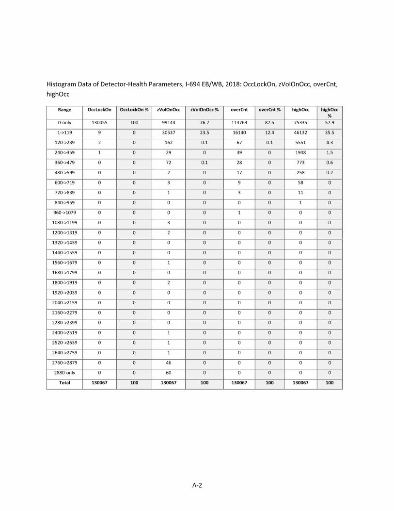
A-2
Histogram Data of Detector-Health Parameters, I-694 EB/WB, 2018: OccLockOn, zVolOnOcc, overCnt,
highOcc
Range OccLockOn OccLockOn % zVolOnOcc zVolOnOcc % overCnt overCnt % highOcc highOcc %
0-only 130055 100 99144 76.2 113763 87.5 75335 57.9
1->119 9 0 30537 23.5 16140 12.4 46132 35.5
120->239 2 0 162 0.1 67 0.1 5551 4.3
240->359 1 0 29 0 39 0 1948 1.5
360->479 0 0 72 0.1 28 0 773 0.6
480->599 0 0 2 0 17 0 258 0.2
600->719 0 0 3 0 9 0 58 0
720->839 0 0 1 0 3 0 11 0
840->959 0 0 0 0 0 0 1 0
960->1079 0 0 0 0 1 0 0 0
1080->1199 0 0 3 0 0 0 0 0
1200->1319 0 0 2 0 0 0 0 0
1320->1439 0 0 0 0 0 0 0 0
1440->1559 0 0 0 0 0 0 0 0
1560->1679 0 0 1 0 0 0 0 0
1680->1799 0 0 0 0 0 0 0 0
1800->1919 0 0 2 0 0 0 0 0
1920->2039 0 0 0 0 0 0 0 0
2040->2159 0 0 0 0 0 0 0 0
2160->2279 0 0 0 0 0 0 0 0
2280->2399 0 0 0 0 0 0 0 0
2400->2519 0 0 1 0 0 0 0 0
2520->2639 0 0 1 0 0 0 0 0
2640->2759 0 0 1 0 0 0 0 0
2760->2879 0 0 46 0 0 0 0 0
2880-only 0 0 60 0 0 0 0 0
Total 130067 100 130067 100 130067 100 130067 100
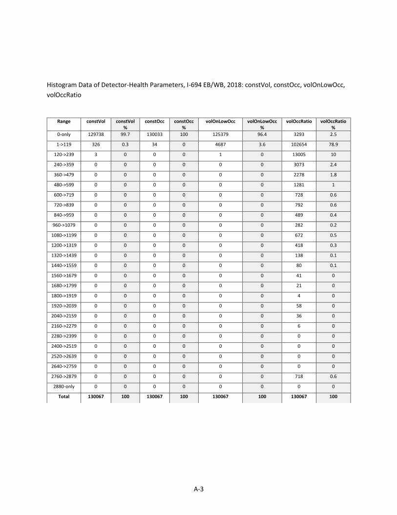
A-3
Histogram Data of Detector-Health Parameters, I-694 EB/WB, 2018: constVol, constOcc, volOnLowOcc,
volOccRatio
Range constVol constVol %
constOcc constOcc %
volOnLowOcc volOnLowOcc %
volOccRatio volOccRatio %
0-only 129738 99.7 130033 100 125379 96.4 3293 2.5
1->119 326 0.3 34 0 4687 3.6 102654 78.9
120->239 3 0 0 0 1 0 13005 10
240->359 0 0 0 0 0 0 3073 2.4
360->479 0 0 0 0 0 0 2278 1.8
480->599 0 0 0 0 0 0 1281 1
600->719 0 0 0 0 0 0 728 0.6
720->839 0 0 0 0 0 0 792 0.6
840->959 0 0 0 0 0 0 489 0.4
960->1079 0 0 0 0 0 0 282 0.2
1080->1199 0 0 0 0 0 0 672 0.5
1200->1319 0 0 0 0 0 0 418 0.3
1320->1439 0 0 0 0 0 0 138 0.1
1440->1559 0 0 0 0 0 0 80 0.1
1560->1679 0 0 0 0 0 0 41 0
1680->1799 0 0 0 0 0 0 21 0
1800->1919 0 0 0 0 0 0 4 0
1920->2039 0 0 0 0 0 0 58 0
2040->2159 0 0 0 0 0 0 36 0
2160->2279 0 0 0 0 0 0 6 0
2280->2399 0 0 0 0 0 0 0 0
2400->2519 0 0 0 0 0 0 0 0
2520->2639 0 0 0 0 0 0 0 0
2640->2759 0 0 0 0 0 0 0 0
2760->2879 0 0 0 0 0 0 718 0.6
2880-only 0 0 0 0 0 0 0 0
Total 130067 100 130067 100 130067 100 130067 100

APPENDIX B
EXAMPLES OF INCIDENT DATA ANALYSES
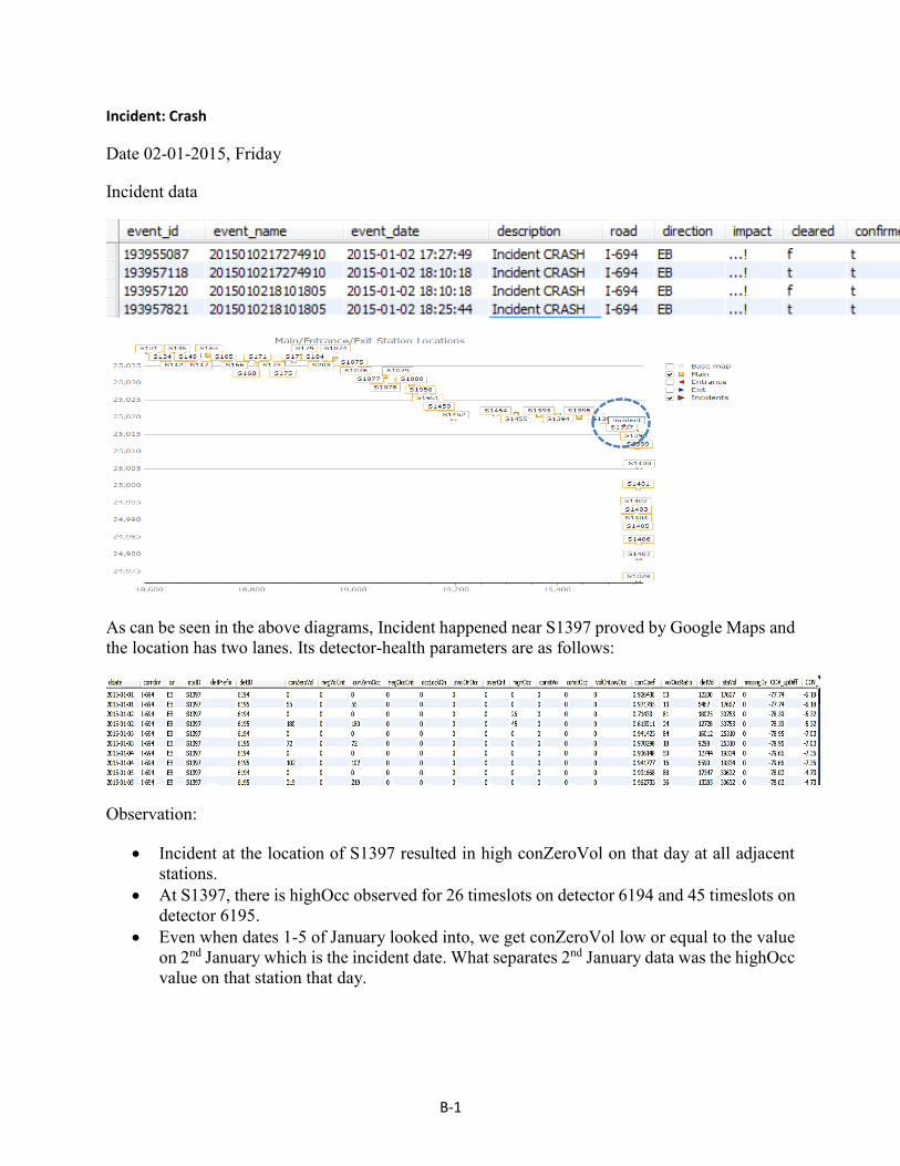
B-1
Incident: Crash
Date 02-01-2015, Friday
Incident data
As can be seen in the above diagrams, Incident happened near S1397 proved by Google Maps and
the location has two lanes. Its detector-health parameters are as follows:
Observation:
Incident at the location of S1397 resulted in high conZeroVol on that day at all adjacent
stations.
At S1397, there is highOcc observed for 26 timeslots on detector 6194 and 45 timeslots on
detector 6195.
Even when dates 1-5 of January looked into, we get conZeroVol low or equal to the value
on 2nd January which is the incident date. What separates 2nd January data was the highOcc
value on that station that day.

B-2
Date 05-01-2015, Monday
Incident data:
'194168394', '2015010522020079', '2015-01-05 22:02:01', 'Incident CRASH', 'I-694', 'EB', '...!',
'f', 't', 'C709', 'Mainline', 'rollover', NULL, '45.0566215515137', '-93.133674621582'
Station S1077, S1078, S1079 and S1080 are near the location of incident. Thus, we analyze their
data trend at adjacent dates 3, 4, 5, 6 of January 2015. The incident occurred on 5th Jan, 2015 at
10pm.
Google Maps of the incident location proves it is S1078.
Observation
The data proves that incident happened on lane 2 of S1078. Hence, the detector on lane 2,
detector ID 4257, shows 166 timeslots of highOcc on 5th January, 2015.

B-3
Date 06-01-2015, Tuesday
Incident data:
'194185364', '2015010522020079', '2015-01-06 04:33:21', 'Incident CRASH', 'I-694', 'EB', '...!', 't',
't', 'C709', 'Mainline', 'rollover', NULL, '45.0566215515137', '-93.133674621582'
According to Google Maps, the location is near S1078 and it has two lanes. We analyze its data
on 5th, 6th, 7th, and 8th of January, 2015.
Observation:
Incident happened on 4am on 6th Jan. 2015. There is no high conZeroVol on S1078 lane
two. However, highOcc value of 25 was observed.

B-4
Date 08-01-2015, Thursday
Incidents:
'194380456', '2015010809204808', '2015-01-08 09:20:48', 'Incident CRASH', 'I-694', 'EB', '.....!.',
'f', 't', 'C7011', 'Mainline', '', NULL, '45.0691528320312', '-93.2802963256836'
'194382064', '2015010809204808', '2015-01-08 09:43:02', 'Incident CRASH', 'I-694', 'EB', '.....!.',
't', 't', 'C7011', 'Mainline', '', NULL, '45.0691528320312', '-93.2802963256836'
The data proves that one incident happened at 9:20am and another at 9:43am over S149 which has
five lanes and five detectors.
Observation:
It can be seen that incidents on 8th Jan 2015 over S149 leads to high highOcc values.

B-5
Incidents:
'194381891', '2015010809410057', '2015-01-08 09:41:02', 'Incident CRASH', 'I-694', 'EB', '..!', 'f',
't', 'C861', 'Exit', '', NULL, '44.9519920349121', '-92.9589004516602'
'194382330', '2015010809410057', '2015-01-08 09:47:50', 'Incident CRASH', 'I-694', 'EB', '..!', 't',
't', 'C861', 'Exit', '', NULL, '44.9519920349121', '-92.9589004516602'
Two incidents happened at S1028 on 8-1-2015 and it shows again high occupancies.

B-6
'194387484', '2015010811182594', '2015-01-08 11:18:26', 'Incident CRASH', 'I-694', 'EB', '..!!',
'f', 't', 'C719', 'Mainline', '', NULL, '45.0322380065918', '-92.9670104980469'
'194389316', '2015010811182594', '2015-01-08 11:49:14', 'Incident CRASH', 'I-694', 'EB', '..!!',
't', 't', 'C719', 'Mainline', '', NULL, '45.0322380065918', '-92.9670104980469'
It can be seen that on 8th Jan, 2015 that two incidents of CRASH occurred, which resulted in
high occupancy values at S1397.
It should also be noted that this incident resulted in a closure of two lanes instead of one in
previous incidents.

B-7
'194390265', '2015010812034773', '2015-01-08 12:03:48', 'Incident CRASH', 'I-694', 'EB', '..!!', 'f',
't', 'C718', 'Mainline', '', NULL, '45.0336532592773', '-92.9810638427734'
'194391100', '2015010812034773', '2015-01-08 12:16:35', 'Incident CRASH', 'I-694', 'EB', '...!', 'f',
't', 'C718', 'Mainline', '', NULL, '45.0336532592773', '-92.9810638427734'
'194397012', '2015010812034773', '2015-01-08 13:47:05', 'Incident CRASH', 'I-694', 'EB', '...!', 't',
't', 'C718', 'Mainline', '', NULL, '45.0336532592773', '-92.9810638427734'
Since S1455, S1393, S1394, S1395, S1396 and S1397 are adjacent, incident at S1396 has effect
on all of them, resulting in high highOcc values at all stations on the date of incident. S1393 was
not working at that time.

B-8
'194390304', '2015010812043678', '2015-01-08 12:04:37', 'Incident CRASH', 'I-694', 'EB', '!..!',
'f', 't', 'C715', 'Mainline', '', NULL, '45.0374145507812', '-93.0440902709961'
'194391513', '2015010812043678', '2015-01-08 12:23:36', 'Incident CRASH', 'I-694', 'EB', '!..!', 't',
't', 'C715', 'Mainline', '', NULL, '45.0374145507812', '-93.0440902709961'
'194391789', '2015010812043678', '2015-01-08 12:27:36', 'Incident CRASH', 'I-694', 'EB', '!..!', 'f',
't', 'C715', 'Mainline', '', NULL, '45.0374145507812', '-93.0440902709961'
'194393899', '2015010812043678', '2015-01-08 13:02:07', 'Incident CRASH', 'I-694', 'EB', '!..!', 't',
't', 'C715', 'Mainline', '', NULL, '45.0374145507812', '-93.0440902709961'
All these incidents happened at S1455. Same patterns as previous are shown. All downstream
stations are affected resulting high occupancies.

B-9
'194390567', '2015010812085843', '2015-01-08 12:08:58', 'Incident CRASH', 'I-694', 'EB', '...!',
'f', 't', 'C706', 'Mainline', '', NULL, '45.0670928955078', '-93.182731628418'
'194390577', '2015010812085843', '2015-01-08 12:09:14', 'Incident CRASH', 'I-694', 'EB', '...!',
't', 't', 'C706', 'Mainline', '', NULL, '45.0670928955078', '-93.182731628418'
The incidents affected occupancies of S203, S184 and S1074.

B-10
'194392694', '2015010812424891', '2015-01-08 12:42:49', 'Incident CRASH', 'I-694', 'EB', '...!!',
'f', 't', 'C704', 'Mainline', '', NULL, '45.0645713806152', '-93.223518371582'
'194404372', '2015010812424891', '2015-01-08 14:45:34', 'Incident CRASH', 'I-694', 'EB', '...!!',
't', 't', 'C704', 'Mainline', '', NULL, '45.0645713806152', '-93.223518371582'
The incidents affected highOcc on S173 and S175.

B-11
Incident: Roadwork
Incidents:
'194787531', '2015011312165690', '2015-01-13 12:16:57', 'Incident ROADWORK', 'I-694', 'EB',
'!!!', 'f', 't', 'C718', 'Exit', '', NULL, '45.0346717834473', '-92.9891204833984'
'194791241', '2015011312165690', '2015-01-13 13:45:11', 'Incident ROADWORK', 'I-694', 'EB',
'!!!', 't', 't', 'C718', 'Exit', '', NULL, '45.0346717834473', '-92.9891204833984'

B-12
As can be seen, highOcc was not affected by ‘Incident Roadwork’ because all lanes were closed
“!!!” in this case. The conZeroVol values seem to be high but it is interesting to note that they are
also high before as well as after the date of incident. Thus, it appears “Incident Roadwork” cause
lane closures and zero volumes.
Incidents:
'195117558', '2015011716115872', '2015-01-17 16:11:59', 'Incident CRASH', 'I-694', 'EB', '!!.....',
'f', 't', 'C701', 'Mainline', '', NULL, '45.0691680908203', '-93.2806396484375'
'195118387', '2015011716115872', '2015-01-17 16:29:43', 'Incident CRASH', 'I-694', 'EB', '!!!....',
'f', 't', 'C701', 'Mainline', '', NULL, '45.0691680908203', '-93.2806396484375'
'195124950', '2015011716115872', '2015-01-17 18:43:38', 'Incident CRASH', 'I-694', 'EB', '!!!....',
't', 't', 'C701', 'Mainline', '', NULL, '45.0691680908203', '-93.2806396484375'

B-13
This CRASH incident happened right after S145 and before S149. High values of highOcc are
mostly visible at the time of the crash incident.
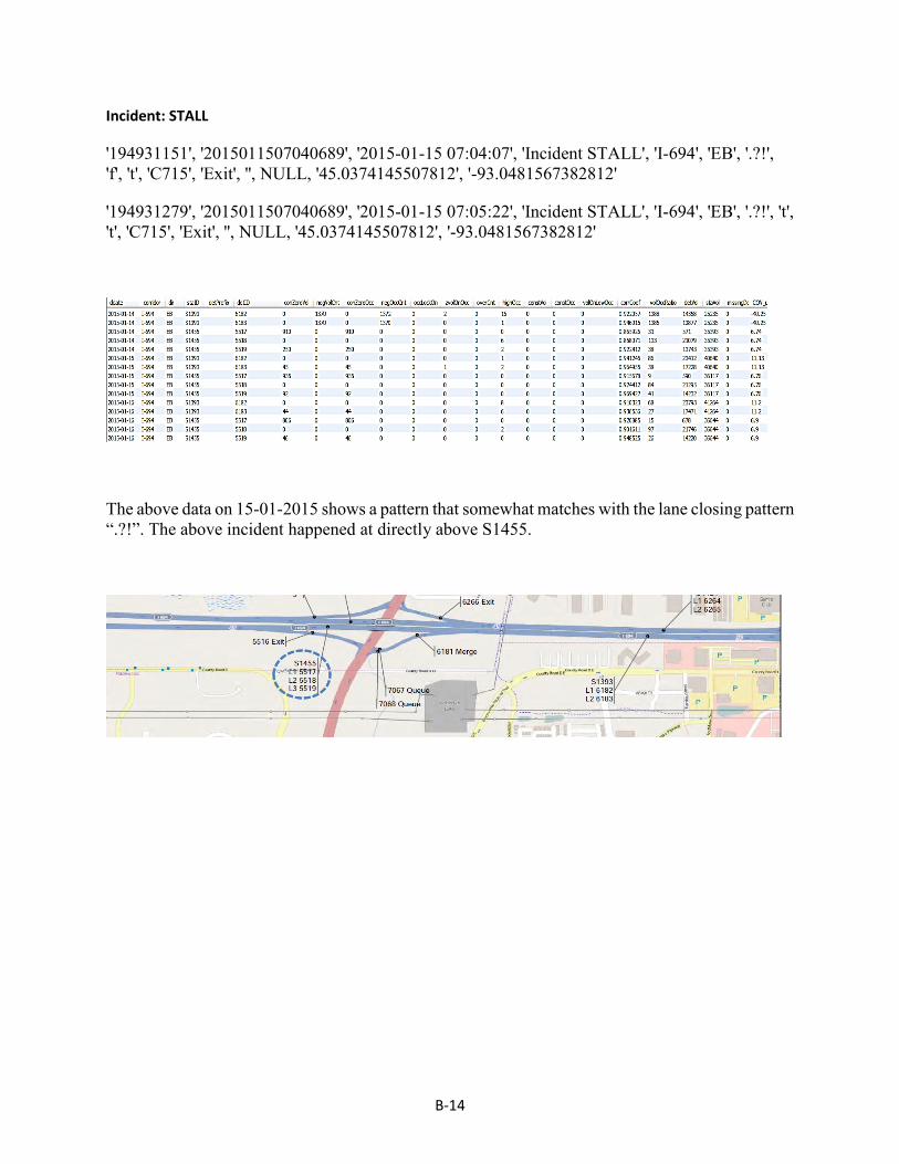
B-14
Incident: STALL
'194931151', '2015011507040689', '2015-01-15 07:04:07', 'Incident STALL', 'I-694', 'EB', '.?!',
'f', 't', 'C715', 'Exit', '', NULL, '45.0374145507812', '-93.0481567382812'
'194931279', '2015011507040689', '2015-01-15 07:05:22', 'Incident STALL', 'I-694', 'EB', '.?!', 't',
't', 'C715', 'Exit', '', NULL, '45.0374145507812', '-93.0481567382812'
The above data on 15-01-2015 shows a pattern that somewhat matches with the lane closing pattern
“.?!”. The above incident happened at directly above S1455.

B-15
'194949148', '2015011510480883', '2015-01-15 10:48:10', 'Incident STALL', 'I-694', 'EB', '..!', 'f',
't', 'C704', 'Exit', '', NULL, '45.0644226074219', '-93.2216796875'
'194952921', '2015011510480883', '2015-01-15 12:17:12', 'Incident STALL', 'I-694', 'EB', '..!', 't',
't', 'C704', 'Exit', '', NULL, '45.0644226074219', '-93.2216796875'
This incident STALL was on S173. Checking both S173 and S175, it does not show any noticeable
increase in health parameters and change in traffic volume.

B-16
Incident: HAZARD
'195061627', '2015011618101286', '2015-01-16 18:10:13', 'Incident HAZARD', 'I-694', 'EB', '.?.',
'f', 't', 'C716', 'Exit', '', NULL, '45.0370445251465', '-93.0217514038086'
'195061729', '2015011618101286', '2015-01-16 18:10:52', 'Incident HAZARD', 'I-694', 'EB', '.?.',
't', 't', 'C716', 'Exit', '', NULL, '45.0370445251465', '-93.0217514038086'
This HAZARD incident happened between S1393 and S1394. It does not show any noticeable
impact on traffic patterns or health parameters.

B-17
Incident: Hazard
'218882207', '2015092011220178', '2015-09-20 11:22:02', 'Incident HAZARD', 'I-694', 'EB', '!!..',
'f', 't', 'C819', 'Mainline', '', NULL, '45.0694808959961', '-93.2978897094727'
'218882209', '2015092011220178', '2015-09-20 11:22:06', 'Incident HAZARD', 'I-694', 'EB', '!!..',
't', 't', 'C819', 'Mainline', '', NULL, '45.0694808959961', '-93.2978897094727'
'218882211', '2015092011220586', '2015-09-20 11:22:06', 'Incident HAZARD', 'I-694', 'EB', '!!..',
'f', 't', 'C819', 'Mainline', 'debris', '2015092011220178', '45.0694808959961', '-93.2978897094727'
'218882297', '2015092011220586', '2015-09-20 11:24:16', 'Incident HAZARD', 'I-694', 'EB', '!!..',
't', 't', 'C819', 'Mainline', 'debris', '2015092011220178', '45.0694808959961', '-93.2978897094727'
This “Incident Hazard” caused lane closures at S134 which has two lanes with detector IDs 681
and 682. Detector 681 was continuously giving 2880 conZeroVol and 0 negVolCnt throughout
two years. It is suspected that there must be construction on that lane, but it needs to be proved
through construction data.
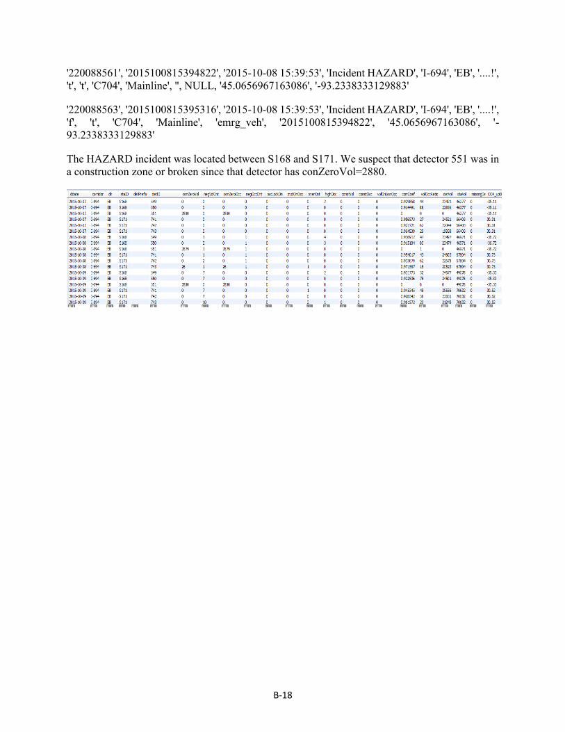
B-18
'220088561', '2015100815394822', '2015-10-08 15:39:53', 'Incident HAZARD', 'I-694', 'EB', '....!',
't', 't', 'C704', 'Mainline', '', NULL, '45.0656967163086', '-93.2338333129883'
'220088563', '2015100815395316', '2015-10-08 15:39:53', 'Incident HAZARD', 'I-694', 'EB', '....!',
'f', 't', 'C704', 'Mainline', 'emrg_veh', '2015100815394822', '45.0656967163086', '-
93.2338333129883'
The HAZARD incident was located between S168 and S171. We suspect that detector 551 was in
a construction zone or broken since that detector has conZeroVol=2880.

B-19
'220365473', '2015101308513143', '2015-10-13 08:51:33', 'Incident HAZARD', 'I-694', 'EB',
'.?....', 'f', 't', 'C702', 'Mainline', '', NULL, '45.0683441162109', '-93.2563629150391'
This HAZARD incident was located between S165 and S163, but the data does not show any sign
of abnormal patterns.

APPENDIX C
TESLA MAINTENANCE LOG DATA ANALYSES

C-1
694-EB, 2015
The following stations in 694-EB had no records in the TESLA Maintenance 2015 and 2016 log,
and thus they are excluded from analyses.
S131, S142, S149, S163, S165, S166, S171, S173, S175, S177, S179, S184, S203, S1074, S1075, S1076,
S1077, S1950, S1951, S1394, S1395, S1396, S1397, S1398, S1399, S1400, S1401, S1402, S1403, S1404,
S1405, S1406, S1407, S1028
The stations that include detectors with one or more maintenance tickets is reviewed one by one.
Station: S134
Detector: 681
It has a TESLA maintenance record in 2015 as follows:
Observations from data:
Detector 681 belongs to station S134 and has a TESLA record on 6/17/2015 as shown above. Data
is reviewed for the date of maintenance, followed by analysis of health parameters for two years.
Observations are summarized below.
S134 has two detectors 681 and 682. 681 had been giving consecutive 0s throughout the
year 2015 and 2016. In contrast, 682 had been working fine during the same time,
producing normal patterns of traffic data.
On 6/17/2015, ‘REPLACE LOOP’ in Ticketstatus can be found from the TESLA log.
In 2015, detector 681 had conZeroVol=2,880 throughout the year except for a few days.
negVolCnt was 1,800 on 12/16/2015 and 1,650 on 12/212015.
It kept the same behavior in 2016. It would either give conZeroVol=2,880 most of the
time or else it gave conZeroVol + negVolCnt =2,880. For example, conZeroVol=1,509
and negVolCnt=1371 on 12/23/2016. The total of conZerovol and negVolCnt was always
near 2,880.
Comments:
Detector 681 gave conZeroVol=2,880 for the most of two years (2015 and 2016) and some
negVolCnt in thousands. The loop was supposed to be replaced on 6/17/2015 but apparently it was
still not replaced or the fix was not successful, because volume counts were either zeros or negative
ones.

C-2
Station: S145
Detectors: 439, 440, 441 and 442
TESLA records were only found in 2016 as follows:
Observations
Maintenance tickets were issued for all four detectors on 3/9/2015 and only detector 442 on
5/3/2015. Data observations are summarized below.
2015
Station S145 has four detectors 439, 440, 441 and 442, in which all of them had been
showing a normal pattern of traffic data in 2015 from 1/1/2015 to 11/29/2015.
After 11/29/2015, volumes become mostly 0’s and conZeroVol=2,880.
negVolCnt was 120 for all detectors on 3/8/2015; 1023 on 8/7/205; 1,023 on 8/7/2015;
and 693 on 12/16/2015.
On 3/9/2015, a ticket was issued for ‘Maintenance Analyze’ for all detectors in S145.
That means that negVolCnt=120 on 3/8/2015 was noticed by MnDOT, from which they
may have placed it in the TESLA maintenance log. On 2nd or 3rd May 2015, data is back
to normal, so the maintenance ticket of detector 442 on 3rd May might have been placed
for confirmation.
2016
conZeroVol becomes large or near 2,880 zeroes starting from 11/30/2015 and it
continues until 1/16/2016.
All detectors or S145 were offline from 1/17/2016 to 7/6/2016.
negVolCnt was 1671 on 7/7/2016, then after which detectors 439 and 440 returned to
normal, whereas detectors 441 and 442 started giving conZeroVol=2,880. This indicates
that detectors 439 and 440 were repaired but not 441 and 442.
On 8/31/2016, the detectors 441 and 442 stop giving conZeroVol=2,880 and returned to
normal. It can be concluded that they finally repaired 441 and 442 in S145.
Comments:

C-3
‘Maintenance Analyze’ tickets were issued on 3/9/2015 and 5/3/2015. Detectors 439 and 440
returned to normal on 7/7/2016, and detectors 441 and 442 on 8/31/2016. This case shows that it
a long delay may be possible between the repair ticket issue and the actual repair.

C-4
Station: S147
Detectors: 3071, 393, 394, 395
Maintenance record was found on 9/16/2015 that detector 394 passed the ‘Operations Test’.
Observations:
2015
Detector 394 gave high conZeroVol (> 2860) until 10/7/2015 and the volume was very
low.
negVolCnt was 120 on 3/8/2015, 1,423 on 5/5/2015, 1,500 on 7-5-2015, 434 on
7/15/2015, then 1,380 on 7/20/2015.
Detector 394 was offline on 5/6/2015 and between 7/16/2015 and 7/20/2015.
2016
conZeroVol seems fine the whole year except on 20 and 21st August, where we get
“conZeroVol > 2600”. Then on 10th and 11th September we get “conZeroVol > 2,600”.
negVolCnt is 120 on 13-3-2016. It is greater than 2,000 on 19th and 20th of June.
Comments
Even though the TESLA data says detector 394 passed ‘Operations Test’ on 9/16/2015, it gave
high conZeroVol (near 2,800) until 10/7/2015. Detector 394 began producing normal data started
staring from 10/8/2015.

C-5
Station: S168
Detectors: 549, 550, 551
It has one maintenance record for detector 551 saying ‘In Repair’ on 9/16/2015.
Observations
2015
Detector 551 kept giving very high conZeroVol (> 2,870) throughout 2015.
Detector 549 and 550 were working fine, and no data was missing throughout 2015.
negVolCnt on detector 551 was 120 on 8th March, 493 on 5th May, and 254 on 15th July.
Volumes of detector 551 were zero throughout 2015.
2016
Detector 551 kept giving very high conZeroVol ( > 2870) throughout 2016.
Detector 549 and 550 were working fine. No data was missing throughout 2016.
For detector 551, negVolCnt was 120 on 13th March, 2,028 on 19th June, and 340 on 20th
June.
Volumes of detector 551 were zero the whole year.
Comment
The detector 551 that was recorded ‘In Repair’ on 16th September 2015 keeps giving conZeroVol
near 2,880 throughout 2015 and 2016. Volumes were zero throughout 2015 and 2016. This
detector is clearly not working in 2015 and 2016, and thus it may never have been repaired, i.e.,
“In Repair” status is probably equivalent to “not repaired yet.”

C-6
Station: S1450
Detectors: 5504, 5505, 5506, 5507, 5508, T6008, T6009, T6010, T6011, T6012
Only one maintenance record was found from detector 5504 for “In Construction” on 4/3/2015.
Observations:
2015
Detector 5504 worked normal from Jan 1 to March 4. Starting March 5, it showed high
conZeroVol and low daily volume (less than 400). Detector 5504 started working normal
after August 23. All other detectors appear to work fine.
negVolCnt was 120 on 8th March for all detectors, 125 on 12th July, 722 on 13th Sept, on,
1,630 on 15th September, 1,416 on 29th September, and 2,190 negVolCnt on 5th October.
Detector 5504 was offline on 14th September and five days between 30th September and
4th October.
Followed by offline, a large negVolCnt value was found in the first online day, i.e., 1,630
on 15th September and 2,190 on 5th October.
Temporary detectors gave no data in 2015. They started giving data from 10th May, 2016.
2016
All detectors work fine until 29th April, 2016 after which only Temporary ‘T’ detectors
work and normal detectors become offline.
negVolCnt was 1,950 on 28th April for all detectors.
Temporary detectors gave 2,072 negVolCnt on 10th May and then started giving normal
data from 11th.
Comments
S1450 has 10 detectors, five of them were temporary and the rest five were regular. Regular
detectors worked fine in 2015 except detector 5504 which had few problems (offline and
negVolCnt). Regular detectors were completely offline starting from April 30, 2016, and then
detectors were switched to temporary detectors and they were online staring from May 10, 2016.
Therefore, there were no detectors activated for 10 days between April 29 – May 9, 2016.
It was observed that negVolCnt was very high just before offline or right after online.

C-7
Station: S1393
Detectors: 6182, 6183
One maintenance record was found for detector 6182 on 10/15/2015:
Observations:
2015
Both detectors were online on January 1, offline until January 13th, and then online again
starting from January 14th and then worked fine for the rest of 2015.
On 1st Jan, 2015 both detectors gave 1396 negVolCnt=1,396. At the first day of online
(January 14), negVolCnt was 1,370 for both detectors.
2016
Detector 6182 started giving conZeroVol=2,880 from January 6th and then until June 26th.
It is strange that it does not give large negVolCnt before and after it starts giving
conZeroVol=2,880.
Starting 27th June, all detectors worked fine and normal.
Comments
The strange thing here is that detector 6182 starts giving 2,880 consecutive zeroes in 2016 and
stops them without the usual pattern of giving large negVolCnt values. It might be due to that the
detectors were placed online near midnight and worked from start.
The TESLA record indicates that a ticket was issued for Lock-On on detector 6182 on October
15, 2015. There were no significant change of data near this log date. However, the data showed
that detector 6182 began working fine starting June 27, 2016, which appears the date of final
repair or recovery from zero volumes.