improve i/o performance and energy eﬃciency in hadoop …

Improve I/O performance and Energy Efficiency in Hadoop Systems

by

Yixian Yang

A dissertation submitted to the Graduate Faculty ofAuburn University

in partial fulfillment of therequirements for the Degree of

Doctor of Philosophy

Auburn, AlabamaAugust 4, 2012

Keywords: MapReduce, Hadoop, HDFS, Data placement, Performance, Energy saving

Copyright 2012 by Yixian Yang

Approved by

Xiao Qin, Chair, Associate Professor of Computer Science and Software EngineeringCheryl Seals, Associate Professor of Computer Science and Software EngineeringDean Hendrix, Associate Professor of Computer Science and Software Engineering

Sanjeev Baskiyar, Associate Professor of Computer Science and Software Engineering

Abstract

MapReduce is one of the most popular distributed computing platforms for the large-

scale data-intensive applications. MapReduce has been applied to many areas of divide-and-

conquer problems like search engines, data mining, and data indexing. Hadoop - developed by

Yahoo - is an open source Java implementation of the MapReduce model. In this dissertation,

we focus on approaches to improving performance and energy efficiency of Hadoop clusters.

We start this dissertation research by analyzing the performance problems of the native

Hadoop system. We observe that Hadoop’s performance highly depends on system settings

like block sizes, disk types, and data locations. A low observed network bandwidth in

a shared cluster raise serious performance issues in the Hadoop system. To address this

performance problem in Hadoop, we propose a key-aware data placement strategy called

KAT for the Hadoop distributed file system (or HDFS, for short) on clusters. KAT is

motivated by our observations that a performance bottleneck in Hadoop clusters lies in

the shuffling stage where a large amount of data is transferred among data nodes. The

amount of transferred data heavily depends on locations and balance of intermediate data

with the same keys. Before Hadoop applications approach to the shuffling stage, our KAT

strategy pre-calculates the intermediate data key for each data entry and allocates data

according to the key. With KAT in place, data sharing the same key are not scattered

across a cluster, thereby alleviating the network performance bottleneck problem imposed

by data transfers. We evaluate the performance of KAT on an 8-node Hadoop cluster.

Experimental results show that KAT reduces the execution times of Grep and Wordcount by

up to 21% and 6.8%, respectively. To evaluate the impact of network interconnect on KAT,

we applied the traffic-shaping technique to emulate real-world workloads where multiple

applications are sharing the network resources in a Hadoop cluster. Our empirical results

ii

suggest that when observed network bandwidth drops down to 10Mbps, KAT is capable

of shortening the execution times of Grep and Wordcount by up to 89%. To make Hadoop

clusters economically and environmentally friendly, we design a new replica architecture that

reduces the energy consumption of HDFS. The core conception of our design is to conserve

power consumption caused by extra data replicas. Our energy-efficient HDFS saves energy

consumption caused by extra data replicas in two steps. First, all disks within in a data node

are separated into two categories: primary copies are stored on primary disks and replica

copies are stored on backup disks. Second, disks archiving primary replica data are kept in

the active mode in most cases; backup disks are placed into the sleep mode. We implement

the energy-efficient HDFS that manages the power states of all disks in Hadoop clusters.

Our approach conserves energy at the cost of performance due to power-state transitions.

We propose a prediction module to hide overheads introduced by the power-state transitions

in backup disks.

iii

Acknowledgments

For this dissertation and other researches at Auburn, I would like to acknowledge the

endless support to me from many persons. It is impossible to finish this dissertation without

them.

First and foremost, I would like to present the appreciation to my advisor, Dr. Xiao

Qin, for his unwavering belief, guidance, and advice on my research. Also, I would like to

thank the effort of Dr. Xiao Qin to revise my dissertation. As my advisor, he did not only

instruct me how to design experiments, develop ideas, and write technical papers, but also

teach me how to communicate with different people and involve in group works.

I would gratefully thank all my committee members, Dr. Dean Hendrix, Dr. Cheryl

Seals, and Dr. Sanjeev Baskiyar, and my university reader, Dr Shiwen Mao from Department

of Electrical and Computer Engineering, for their valuable suggestions and advices on my

research and dissertation. My thanks also go to Dr. Kai Chang and Dr. David Umphress

for their constructive suggestions on my Ph.D. program.

I would like to name all the members in my group. They are Xiaojun Ruan, Zhiyang

Ding, Jiong Xie, Shu Yin, Jianguo Lu, Yun Tian, James Major, Ji Zhang and Xunfei Jiang.

It would be my fortune and my honor to work with such great persons. Also, it would be

my pleasure to name my friends in Auburn. They are Rui Xu, Sihe Zhang, Jiawei Zhang,

Suihan Wu, Qiang Gu, Jingshan Wang, Jingyuan Xiong, Fan Yang, Tianzi Guo, and Min

Zheng.

My deepest gratitude goes to my parents Jinming Yang and Fuzhen Cui for their years

of selfless support. Without them, I would never have a chance to do my research and finish

the dissertation in Auburn. They also gave me such freedom on the choice for my future

career.

iv

At the end, I would like to thank my girlfriend, Ying Zhu, staying by my side during

the toughest days. It was her who encouraged me to fight against myself with calm sense

and strengthen conviction. Her love becomes my power to conquer all problems.

v

Table of Contents

Abstract . . . . . . . . . . . . . . . . . . . . . . . . . . . . . . . . . . . . . . . . . . . ii

Acknowledgments . . . . . . . . . . . . . . . . . . . . . . . . . . . . . . . . . . . . . . iv

List of Figures . . . . . . . . . . . . . . . . . . . . . . . . . . . . . . . . . . . . . . . ix

List of Tables . . . . . . . . . . . . . . . . . . . . . . . . . . . . . . . . . . . . . . . . xiii

1 Introduction . . . . . . . . . . . . . . . . . . . . . . . . . . . . . . . . . . . . . . 1

1.1 Data Location And Performance Problem . . . . . . . . . . . . . . . . . . . 1

1.2 Replica Reliability And Energy Efficiency Problem . . . . . . . . . . . . . . 2

1.3 Contribution . . . . . . . . . . . . . . . . . . . . . . . . . . . . . . . . . . . . 3

1.4 Organization . . . . . . . . . . . . . . . . . . . . . . . . . . . . . . . . . . . 4

2 Hadoop Performance Profiling and Tuning . . . . . . . . . . . . . . . . . . . . . 5

2.1 Introduction . . . . . . . . . . . . . . . . . . . . . . . . . . . . . . . . . . . . 5

2.2 Background and Previous Work . . . . . . . . . . . . . . . . . . . . . . . . . 7

2.2.1 Log Structured File System . . . . . . . . . . . . . . . . . . . . . . . 8

2.2.2 SSD . . . . . . . . . . . . . . . . . . . . . . . . . . . . . . . . . . . . 8

2.3 Hadoop Experiments And Solution Analysis . . . . . . . . . . . . . . . . . . 9

2.3.1 Experiments Environment . . . . . . . . . . . . . . . . . . . . . . . . 9

2.3.2 Experiment Results Analysis . . . . . . . . . . . . . . . . . . . . . . . 10

2.3.3 HDD and SSD Hybrid Hadoop Storage System . . . . . . . . . . . . 17

2.4 Summary . . . . . . . . . . . . . . . . . . . . . . . . . . . . . . . . . . . . . 18

3 Key-Aware Data Placement Strategy . . . . . . . . . . . . . . . . . . . . . . . . 20

3.1 Introduction . . . . . . . . . . . . . . . . . . . . . . . . . . . . . . . . . . . . 20


3.2.1 MapReduce . . . . . . . . . . . . . . . . . . . . . . . . . . . . . . . . 25

vi

3.2.2 Hadoop and HDFS . . . . . . . . . . . . . . . . . . . . . . . . . . . . 26

3.3 Performance Analysis of Hadoop Clusters . . . . . . . . . . . . . . . . . . . . 28

3.3.1 Experimental Setup . . . . . . . . . . . . . . . . . . . . . . . . . . . . 28

3.3.2 Performance Impacts of Small Blocks . . . . . . . . . . . . . . . . . . 28

3.3.3 Performance Impacts of Network Interconnects . . . . . . . . . . . . . 31

3.4 Key-Aware Data Placement . . . . . . . . . . . . . . . . . . . . . . . . . . . 34

3.4.1 Design Goals . . . . . . . . . . . . . . . . . . . . . . . . . . . . . . . 34

3.4.2 The Native Hadoop Strategy . . . . . . . . . . . . . . . . . . . . . . . 38

3.4.3 Implementation Issues . . . . . . . . . . . . . . . . . . . . . . . . . . 39

3.5 Experimental Results . . . . . . . . . . . . . . . . . . . . . . . . . . . . . . . 43

3.5.1 Experimental Setup . . . . . . . . . . . . . . . . . . . . . . . . . . . . 44

3.5.2 Scalability . . . . . . . . . . . . . . . . . . . . . . . . . . . . . . . . . 45

3.5.3 Network Traffic . . . . . . . . . . . . . . . . . . . . . . . . . . . . . . 47

3.5.4 Block Size and Input Files Size . . . . . . . . . . . . . . . . . . . . . 49

3.5.5 Stability of KAT . . . . . . . . . . . . . . . . . . . . . . . . . . . . . 55

3.5.6 Analysis of Map and Reduce Processes . . . . . . . . . . . . . . . . . 59

3.6 Summary . . . . . . . . . . . . . . . . . . . . . . . . . . . . . . . . . . . . . 64

4 Energy-Efficient HDFS Replica Storage System . . . . . . . . . . . . . . . . . . 65

4.1 Introduction . . . . . . . . . . . . . . . . . . . . . . . . . . . . . . . . . . . . 66

4.1.1 Motivation . . . . . . . . . . . . . . . . . . . . . . . . . . . . . . . . . 66


4.2.1 RAID Based Storage Systems . . . . . . . . . . . . . . . . . . . . . . 69

4.2.2 Power Savings in Clusters . . . . . . . . . . . . . . . . . . . . . . . . 70

4.2.3 Disk Power Conservation . . . . . . . . . . . . . . . . . . . . . . . . . 71

4.3 Design and Implementation Issues . . . . . . . . . . . . . . . . . . . . . . . . 71

4.3.1 Replica Management . . . . . . . . . . . . . . . . . . . . . . . . . . . 72

4.3.2 Power Management . . . . . . . . . . . . . . . . . . . . . . . . . . . . 74

vii

4.3.3 Performance Optimization . . . . . . . . . . . . . . . . . . . . . . . . 79

4.4 Experimental Results . . . . . . . . . . . . . . . . . . . . . . . . . . . . . . . 82

4.4.1 Experiments Setup . . . . . . . . . . . . . . . . . . . . . . . . . . . . 82

4.4.2 What Do We Measure . . . . . . . . . . . . . . . . . . . . . . . . . . 83

4.4.3 Results Analysis . . . . . . . . . . . . . . . . . . . . . . . . . . . . . 84

4.4.4 Discussions and Suggestions . . . . . . . . . . . . . . . . . . . . . . . 87

4.5 Summary . . . . . . . . . . . . . . . . . . . . . . . . . . . . . . . . . . . . . 87

5 Conclusion . . . . . . . . . . . . . . . . . . . . . . . . . . . . . . . . . . . . . . . 89

5.1 Observation and Profiling of Hadoop Clusters . . . . . . . . . . . . . . . . . 89

5.2 KAT Data Placement Strategy for Performance Improvement . . . . . . . . 90

5.3 Replica Based Energy Efficient HDFS Storage System . . . . . . . . . . . . . 91

5.4 Summary . . . . . . . . . . . . . . . . . . . . . . . . . . . . . . . . . . . . . 92

6 Future Works . . . . . . . . . . . . . . . . . . . . . . . . . . . . . . . . . . . . . 93

6.1 Data Placement with Application Disclosed Hints . . . . . . . . . . . . . . . 93

6.2 Trace Based Prediction . . . . . . . . . . . . . . . . . . . . . . . . . . . . . . 93

Bibliography . . . . . . . . . . . . . . . . . . . . . . . . . . . . . . . . . . . . . . . . 95

viii

List of Figures

2.1 Wordcount Response Time of the Hadoop Systems With Different Block Sizes

and Input Sizes . . . . . . . . . . . . . . . . . . . . . . . . . . . . . . . . . . . . 10

2.2 Wordcount Response Time of the Hadoop Systems With Different Block Sizes

and Different Number of Tasks . . . . . . . . . . . . . . . . . . . . . . . . . . . 11

2.3 Wordcount I/O Records on Machine Type I with 1GB Input Splited to 64MB

Blocks . . . . . . . . . . . . . . . . . . . . . . . . . . . . . . . . . . . . . . . . . 11


Blocks . . . . . . . . . . . . . . . . . . . . . . . . . . . . . . . . . . . . . . . . . 12


Blocks . . . . . . . . . . . . . . . . . . . . . . . . . . . . . . . . . . . . . . . . . 12


Blocks . . . . . . . . . . . . . . . . . . . . . . . . . . . . . . . . . . . . . . . . . 12

2.7 Wordcount I/O Records on Machine Type I with 1GB Input Splited to 1GB Blocks 13


Blocks . . . . . . . . . . . . . . . . . . . . . . . . . . . . . . . . . . . . . . . . . 13


Blocks . . . . . . . . . . . . . . . . . . . . . . . . . . . . . . . . . . . . . . . . . 13

ix


Blocks . . . . . . . . . . . . . . . . . . . . . . . . . . . . . . . . . . . . . . . . . 14


Blocks . . . . . . . . . . . . . . . . . . . . . . . . . . . . . . . . . . . . . . . . . 14

2.12 Wordcount I/O Records on Machine Type I with 2GB Input Splited to 1GB Blocks 14

2.13 CPU Utilization of Wordcount Executing on Type V . . . . . . . . . . . . . . . 15

2.14 Read Records of Wordcount Executing on Type V . . . . . . . . . . . . . . . . 16

2.15 Write Records of Wordcount Executing on Type V . . . . . . . . . . . . . . . . 16

2.16 CPU Utilization of Wordcount Executing on Type VI . . . . . . . . . . . . . . . 17

2.17 Read Records of Wordcount Executing on Type VI . . . . . . . . . . . . . . . . 17

2.18 Write Records of Wordcount Executing on Type VI . . . . . . . . . . . . . . . . 18

2.19 HDD and SSD Hybrid Storage System for Hadoop Clusters . . . . . . . . . . . 18

2.20 The Wordcount Response Time for Different Types of Storage Disks . . . . . . 19

3.1 An Overview of MapReduce Model [14] . . . . . . . . . . . . . . . . . . . . . . . 26

3.2 CPU utilization for wordcount with block size 64MB . . . . . . . . . . . . . . . 29

3.3 CPU utilization for wordcount with block size 128MB . . . . . . . . . . . . . . 30

3.4 CPU utilization for wordcount with block size 256MB . . . . . . . . . . . . . . 30

3.5 Execution times of WordCount under good and poor network conditions; times

are measured in Second. . . . . . . . . . . . . . . . . . . . . . . . . . . . . . . . 32

x

3.6 Amount of data transferred among data nodes running WordCount under good

and poor network conditions; data size is measured in GB. . . . . . . . . . . . . 33

3.7 Data placement strategy in the native Hadoop. Four key-value pairs (i.e., two

(1, ∗) and two (2, ∗)) are located on node A; four key-value pairs (i.e., two (1, ∗)

and two (2, ∗)) are located on node B. During the shuffling phase, the two (1, ∗)

pairs on node B are transferred to node A; the two (2, ∗) pairs on node A are

delivered to node B. . . . . . . . . . . . . . . . . . . . . . . . . . . . . . . . . . 36

3.8 KAT: a key-based data placement strategy in Hadoop. KAT assigns the four

(1, ∗) key-value pairs to node A and assigns the four (2, ∗) key-value pairs to node

B. This data-placement decision eliminates the network communication overhead

incurred in the shuffling phase. . . . . . . . . . . . . . . . . . . . . . . . . . . . 37

3.9 The architecture of a Hadoop cluster [34]. The data distribution module in HDFS

maintains one queue on namenode to manage data blocks with a fixed size. . . . 42

3.10 Execution Times of Grep and Wordcount on the Hadoop cluster. The number of

data nodes is set to 2, 4, and 8, respectively. . . . . . . . . . . . . . . . . . . . . 46

3.11 Network traffics of the Wordcount and Grep Applications. . . . . . . . . . . . . 48

3.12 Grep with 2GB input in 1Gbps network . . . . . . . . . . . . . . . . . . . . . . 49



3.15 Grep with 2GB input in 10Mbps network . . . . . . . . . . . . . . . . . . . . . 51



xi

3.18 Wordcount with 2GB input in 1Gbps network . . . . . . . . . . . . . . . . . . . 52



3.21 Wordcount with 2GB input in 10Mbps network . . . . . . . . . . . . . . . . . . 54



3.24 Standard deviation of Grep in 1Gbps network . . . . . . . . . . . . . . . . . . . 56

3.25 Standard deviation of Grep in 10Mbps network . . . . . . . . . . . . . . . . . . 56

3.26 Standard deviation of Wordcount in 1Gbps network . . . . . . . . . . . . . . . . 57

3.27 Standard deviation of Wordcount in 10Mbps network . . . . . . . . . . . . . . . 57

3.28 Wordcount Execution process of Traditional Hadoop with 1Gbit/s Bandwidth . 59

3.29 Wordcount Execution process of Traditional Hadoop with 10Mbit/s Bandwidth 60

3.30 Wordcount Execution process of KAT-Enabled Hadoop with 1Gbit/s Bandwidth 60

3.31 Wordcount Execution process of KAT-Enabled Hadoop with 10Mbit/s Bandwidth 61

4.1 Architecture Design of the Energy-Efficient HDFS . . . . . . . . . . . . . . . . . 72

4.2 Data Flow of Copying Data into HDFS . . . . . . . . . . . . . . . . . . . . . . . 73

4.3 Wordcount execution times of the energy efficient HDFS and the native HDFS. 84

4.4 Wordcount power consumptions of energy efficient HDFS and the native HDFS. 85

4.5 Power consumptions of Wordcount on energy-efficient HDFS and the native HDFS. 86

xii

List of Tables

2.1 Comparison of SSD and HDD [45] . . . . . . . . . . . . . . . . . . . . . . . . . 8

2.2 Different Configuration Types of Computing Nodes . . . . . . . . . . . . . . . . 9

3.1 Computing Nodes Configurations . . . . . . . . . . . . . . . . . . . . . . . . . . 28

3.2 Configurations of name and data nodes in the Hadoop cluster. . . . . . . . . . . 45

4.1 Energy-Efficient HDFS Cluster Specifications . . . . . . . . . . . . . . . . . . . 82

xiii

Chapter 1

Introduction

In the past decade, cluster computing model has been deployed to support a variety

of large-scale data-intensive applications. These applications supported out lives in forms

of, for example, the search engines, web indexing, social network data mining and cloud

storage systems. The performance and the energy consumption are two major concerns in

the designs of computation models.

In recent years, MapReduce becomes a excellent computing model in terms of perfor-

mance. It has good scalability and easy usabilities. The programer doesn’t need complicate

distributed programming knowledge to write the parallel program. And MapReduce is guar-

anteed fully fault tolerance. However, MapReduce model is an ”all purpose” computation

model that is not tailored for any particular applications. As its most successful implemen-

tation, Hadoop represents the performance and the energy efficiency of MapReduce model.

The cluster storage system is a essential building block of Hadoop computing clusters.

It supports the distributed computing algorithms as well as the data reliability. On the

other hand, the distributed cluster storage systems cost a huge amount of the energy too.

That means that a better designed storage system can not only improve the performance of

Hadoop systems, but also save a huge amount of power consumptions. The problem can be

divided into two main issues.

1.1 Data Location And Performance Problem

Although most of people improve the Hadoop performance through better scheduling

the tasks and utilizing the CPUs and memories, we want to find the bottleneck and improve

1

it on disk I/Os. Based on what we observed, the locations of the data are divided into two

different kinds, the type of disks and the physical locations related to data nodes.

Two kinds of disks can be utilized as options, the hard drive disks and solid state disks.

The hard drive disks have very good sequential read and write performance. Comparing to

the hard drive disks, SSD has better random read performance but shorter life spans since

the SSDs have limits on the number of writes. According to the Hadoop process, there are

two different kinds of the data too, the input data and the intermediate data. Normally,

both of these data will be accessed randomly. The difference is that the input data will

be read multiple times while the intermediate data will be read and modified many times.

The access natures of different kinds of data indicate the different access patterns, and these

patterns fit to different kinds of disk attributes. So locating the data on the right type of

disks can improve the performance and fully utilize these disks.

The data locations on different data nodes affect the performance as well. The prelimi-

nary results shows multiple replica copies improve the performance and reduce the network

data transfer. Data nodes process more data replica on the local machine when the number

of replica is greater than one. Actually, the network data transfers include the intermediate

data and the original input data. If the cluster is homogenous, the input data locations do

not slow down the performance as long as the data is well balanced. However, the interme-

diate data is required to be transferred during the shuffling stage so that the intermediate

data with the same key can be processed by the same reducer on a data node. This will be

an issue that slow down the performance.

1.2 Replica Reliability And Energy Efficiency Problem

Using replica is a secure method to make the data reliable. The more replica copies are

used, more reliable the data is. Hadoop has rollback mechanism that can recover from a

failed process or even a whole data node. This feature is called fault tolerance in Hadoop

design. The cost of this is paying more for the disk spaces and the power consumptions of

2

these spaces. And it is not only for the economical reason but also for the environmental

consideration to save the energy. There is a tradeoff between the number of replicas and

their energy consumptions. Our goal is to find a solution that can still keep all the copies of

replica while the energy consumption is reduced.

1.3 Contribution

To solve the problem mentioned above, we focus our research on the Hadoop Distributed

File System (HDFS). Our contribution consist with three different parts, the observation,

performance improvement, and energy efficient HDFS.

• We test the Hadoop with different configurations and the combination of different type

of disks. The results show that using the correct disk type and configuration settings

improves the performance. The I/O utilization records show that Hadoop doesn’t have

very intensive reads or writes during the map phase. This becomes the reason that

why we can save the energy from storage system and maintain the same throughput.

• For certain applications whose intermediate key doesn’t require complicate calcula-

tions, we developed a new data placement strategy involving the intermediate key pre-

calculation before the data is distributed to data nodes. When the data is processed

by local mappers, the intermediate data with the same key resides on the same data

nodes. And there is no need to shuffle the data between data nodes. When the network

condition is not very well, this strategy can improve the performance dramaticlly.

• Based on the observations, we propose a new data location strategy to divid the replicas

into two categories, the primary copies and backup copies. And these two kinds of

data are stored separately on different storage disks. At the most of time, the backup

replica disks are kept in standby mode for the energy saving purpose. When the extra

copies are needed, the backup replica disks are waked up to provide services. In this

3

strategy, we save most of the energy consumed by storage system. For its performance

drawbacks, we add the prediction module to minimize the disk wake-up delays.

1.4 Organization

The rest of this dissertation will be organized as following structures.

In Chapter 2, we do a lot of experiments with different system settings as well as

hardware configurations.

Based on the observations in the Chapter 2, the key-aware data placement strategy is

proposed in Chapter 3 to improve the I/O performance of Hadoop systems.

In Chapter 4, we present the energy efficient HDFS design which can save the power

consumptions from the data storage redundancies in current HDFS.

Finally, Chapter 5 summarizes the contributions in this dissertation and Chapter 6

reveals the future research directions for this dissertation.

4

Chapter 2

Hadoop Performance Profiling and Tuning

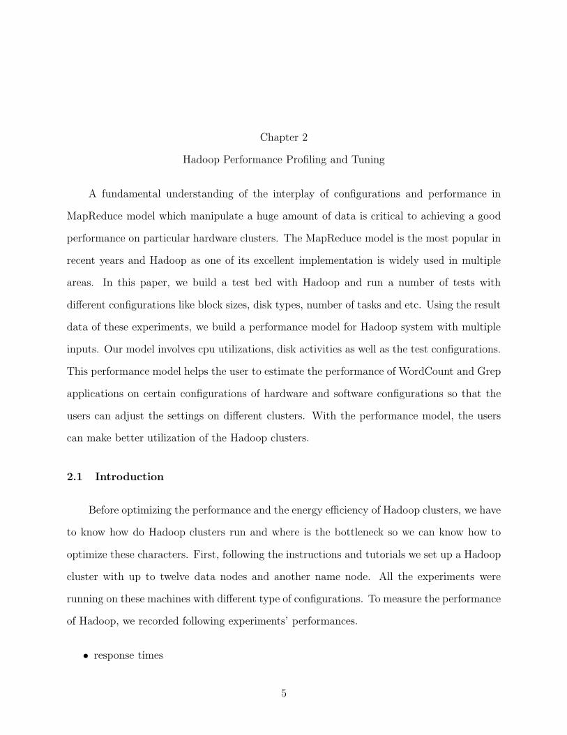
A fundamental understanding of the interplay of configurations and performance in

MapReduce model which manipulate a huge amount of data is critical to achieving a good

performance on particular hardware clusters. The MapReduce model is the most popular in

recent years and Hadoop as one of its excellent implementation is widely used in multiple

areas. In this paper, we build a test bed with Hadoop and run a number of tests with

different configurations like block sizes, disk types, number of tasks and etc. Using the result

data of these experiments, we build a performance model for Hadoop system with multiple

inputs. Our model involves cpu utilizations, disk activities as well as the test configurations.

This performance model helps the user to estimate the performance of WordCount and Grep

applications on certain configurations of hardware and software configurations so that the

users can adjust the settings on different clusters. With the performance model, the users

can make better utilization of the Hadoop clusters.

2.1 Introduction

Before optimizing the performance and the energy efficiency of Hadoop clusters, we have

to know how do Hadoop clusters run and where is the bottleneck so we can know how to

optimize these characters. First, following the instructions and tutorials we set up a Hadoop

cluster with up to twelve data nodes and another name node. All the experiments were

running on these machines with different type of configurations. To measure the performance

of Hadoop, we recorded following experiments’ performances.

• response times

5

• I/O throughputs

• CPU utilizations

• Network traffics

The response times represent the core of performance, cluster speed. The most impor-

tant aspect people concerned is the time used. All we want to do is shorting the response

time while the cost of hardware is limited. That’s the reason why to optimizing the per-

formance through different way. Although we admit that using better scheduling algorithm

can improve the performance, the easiest way to achieve that is changing the system settings

according to the hardware configurations.

I/O throughputs is another important index for utilizations of storage systems. As

all we know, for those I/O intensive applications, the storage system could be the biggest

bottleneck of the whole system. So it is important to make sure all the potentials of the

storage system are utilized.

CPU utilization is definitely an important index of the performance. CPUs are the core

of computing, and their speeds and utilizations directly reflect on the response times and

total system performance. And CPUs now can have at least two cores and these cores run

parallel. Fully utilization of such complicated architecture is not a simple job.

The performance is decided by not only single machine performance but also the com-

munications between different nodes. Sometimes the network conditions have influences on

the performances too. To minimize this part of impacts, a node should send only necessary

messages and data. Another solution is to use faster network like infiniband networks [20].

However, it is not every one that has an infiniband installed because it is expensive and

requires hardware deployment. So minimizing the communication traffic is the most efficient

solution to this problem.

In this chapter, we have done a lot of tests to find the bottlenecks and possible solutions.

From the experiment results, we observed that the disk I/O is not efficient and the potentials

6

of the disk is not well utilized. These observations provide important clues for our works in

next two chapters. In this chapter, we also propose a easy solution to utilize the solid state

disk to improve the I/O speed and shows the evidence that SSD improve the overall system

performance.

2.2 Background and Previous Work

This chapter is about knowing the system and testing the benchmarks first. Then it

comes with some solutions that can improve the performance quick with less effort. There

are many models have been created for Hadoop performance and involve a lot of benchmark

testing. These evidence of the Hadoop performance on different clusters provide us an

example which we can compare to using our own data. And some of these models also

provide hints to improve the performance of Hadoop clusters and data intensive applications.

After google publish the MapReduce computational architecture, a variety of efforts have

been put into the research to understand the performance trends in this systems [17, 12, 49].

The problems in this system have been identified too. For example, there are overheads

between each tasks caused by input requests for shared resources and CPU content exchanges.

Besides the execution time, these tasks may experience two types of delay: (1) queuing delays

due to contention at shared resources, and (2) synchronization delays due to precedence

constraints among tasks [30]. To solve the problems, multiple solutions are proposed. The

most efficient method to improve the performance is adjusting the configurations in the

Hadoop system. In these researches, we found that enabling the JVM reuse eliminate the

Java task initiations before each task starts [47]. When the number of blocks is huge, it saves

a significant time period from the whole process. Based on the optimizations, the literature

is rich of modeling techniques to predict performance of workloads that do not exhibit

synchronization delays. In particular, Mean Value Analysis (MVA) [32] has been applied to

predict the average performance of several applications in various scenarios [23, 48]. Among

these models, it is the massive experiment data that supports their model and prediction

7

results. In this chapter, we are going to follow the same route running massive experiments

and finding solutions from these experiment results in the following chapters.

2.2.1 Log Structured File System

Log structured file system was proposed first in 1988 by John and Fred. And the design

and implementation details are introduced in Mendel and John’s paper in 1992 [39]. The

purpose of log structured file system is to improve the sequential writes’ throughput. Con-

ventional file systems locate files for better read and write performances over the magnetic

and optical disks. The log structured file systems intend to write the file sequentially to the

disks like a log. Log structured file systems save the seek time for disk writes of sequence

files. We tried this file system to improve the I/O performance on Hadoop clusters. However,

it doesn’t work with our Hadoop cluster. The further investigation is needed on Hadoop disk

access patterns.

2.2.2 SSD

A solid state disk refers to the storage device using integrated circuit memories. The SSD

is well known for high speed of random accesses for the data. A comprehensive comparison

table can be found on the wikipedia page [44]. Table 2.2.2 is a short version from sandisk

support website. From the table we observe that SSDs outperform HDDs from several aspect

like power consumption and average access time. There are a number of researches focusing

on improving disk access rate using SSD.

HDD SSDStorage Capacity Up to 4TB Up to 2TB (64 to 256GB are

common sizes for less cost)Avg Access Time 11ms 0.11ms

Noise 29dB NonePower Consumption 20 Watts 0.38 Watts

Table 2.1: Comparison of SSD and HDD [45]

8

2.3 Hadoop Experiments And Solution Analysis

In this section, we will run comprehensive experiments with different hardware and

software configurations. The experiments will keep the records of variety of performance

indexes like CPU utilizations, I/O throughputs and response times. Based on these numbers,

we analysis the system bottleneck and propose possible solutions to improve our Hadoop

system.

2.3.1 Experiments Environment

The experiments run at following hardware configurations in Table 2.3.1. There are

two type of machine with different CPUs. We configure these two machines with different

number of memories and different types of disk. There are two reasons to use different

number of memories. First, we want to test the performance with different input/memory

ratio. Second, for the efficiency of experiments, we cut both the input and memory to

short the response time since the input size has more influences on the response times. In

our experiments, we also involve the SSD based on its great performance in others’ research

mentioned in Section 2.2. Based on all the experiments, we adjust the software configurations

and propose a hybrid disk solution for both performance and reliability. And we will list the

performance results of the WordCount benchmark in Hadoop example packages.

ComputingNode

CPU Memory Disk

Type I Intel 3.0GHz Duo-Core Processor 2GByte Seagate SATA HDDType II Intel 3.0GHz Duo-Core Processor 4GByte Seagate SATA HDDType III Intel 2.4 GHz Quad-Core Processor 2GByte Seagate SATA HDDType IV Intel 2.4 GHz Quad-Core Processor 4GByte Seagate SATA HDDType V Intel 3.0GHz Duo-Core Processor 2GByte Corsair F40A SSDType VI Intel 2.4 GHz Quad-Core Processor 2GByte Corsair F40A SSDType VII Intel 3.0GHz Duo-Core Processor 2GByte Corsair F40A SSD

& Seagate SATA HDD

Table 2.2: Different Configuration Types of Computing Nodes

9

!"

#!"

$!!"

$#!"

%!!"

%#!"

&!!"

&#!"

'!!"

'#!"

#!!"

('" $%)" %#(" #$%" $!%'"

!"#$%&#"'()*

"'+)&'#",%&-.'

/0-%%$'12%,3'4)5"'+61.'

$*+",-./0"

%*+",-./0"

Figure 2.1: Wordcount Response Time of the Hadoop Systems With Different Block Sizesand Input Sizes

2.3.2 Experiment Results Analysis

The first group of tests we did is measure the performances with different Hadoop block

sizes and input file sizes. Figure 2.1 shows the response times of the word count benchmark

with two different input file sizes and five different Hadoop block sizes on machine type I

in table 2.3.1. The results shows that, when the ratio of the input size and the block size

is greater than the number of cores in the CPU, the response time increases dramatically

since the CPU is not fully utilized of every core in it. And the time of processing 2GB input

files is slightly shorter than two times of processing 1GB input files. We can argue that

bigger file size could reduce the ratio of initialization and job processing. At last, the figure

shows the response times of using large blocks is shorter than using the small ones as long

as the ratio of input and block sizes is not exceed the number of CPU cores. Figure 2.2 gives

another evidence supporting the analysis above on a Quad-Core machine. It can improve

the performance that using larger block sizes within the limit. And the number of mappers

affect the performance according to the number of CPU cores.

10

!"

#!"

$!!"

$#!"

%!!"

%#!"

&!!"

&#!"

'!!"

'#!"

#!!"

('" $%)" %#(" #$%"

!"#$%&#"'()*

"'+#",%&-.'

/0-%%$'12%,3'4)5"'+61.'

%"*+,"%"-./01."

'"*+,"%"-./01."

'"*+,"'"-./01."

Figure 2.2: Wordcount Response Time of the Hadoop Systems With Different Block Sizesand Different Number of Tasks

0

2

4

6

8

10

12

14

0 50 100 150 200 250

I/O (MB/s)

Time (in seconds)

Read Write

Figure 2.3: Wordcount I/O Records on Machine Type I with 1GB Input Splited to 64MBBlocks

11

0

1

2

3

4

5

6

7

8

9

10

0 50 100 150 200 250

I/O (MB/s)

Time (in seconds)

Read Write


0

1

2

3

4

5

6

7

8

9

0 50 100 150 200 250

I/O (MB/s)

Time (in seconds)

Read Write


0

2

4

6

8

10

12

14

16

18

20

0 50 100 150 200 250

I/O (MB/s)

Time (in seconds)

Read Write


12

0

2

4

6

8

10

12

14

16

18

20

0 50 100 150 200 250 300 350 400

I/O (MB/s)

Time (in seconds)

Read Write

Figure 2.7: Wordcount I/O Records on Machine Type I with 1GB Input Splited to 1GBBlocks

0

2

4

6

8

10

12

14

16

18

20

0 50 100 150 200 250 300 350 400 450 500

I/O (MB/s)

Time (in seconds)

Read Write


0

2

4

6

8

10

12

14

0 50 100 150 200 250 300 350 400 450

I/O (MB/s)

Time (in seconds)

Read Write


13

0

2

4

6

8

10

12

14

0 50 100 150 200 250 300 350 400 450

I/O (MB/s)

Time (in seconds)

Read Write


0

2

4

6

8

10

12

14

16

18

20

0 50 100 150 200 250 300 350 400 450

I/O (MB/s)

Time (in seconds)

Read Write


0

2

4

6

8

10

12

14

16

18

20

0 50 100 150 200 250 300 350 400 450

I/O (MB/s)

Time (in seconds)

Read Write

Figure 2.12: Wordcount I/O Records on Machine Type I with 2GB Input Splited to 1GBBlocks

14

In last paragraph, we have analyzed the reason and trend of the Hadoop performance.

To backup our results, Figure 2.3-Figure 2.12 present the I/O records of the results in

Figure 2.1. From these records, we have two observations.

• The average of I/O access rate is much lower than the maximum throughput of the

disks. This observation tell us that the WordCount example in the Hadoop package

is a computation intensive application other than a data intensive application. If we

can improve the performance of computation intensive applications through the disk

accesses, then data intensive applications can benefit much more from the solution.

• Between each task runs, the I/O access rate suddenly drops due to the content switches

and disk seek and rotation delay.

These two observations inspire us to propose the hybrid storage system for Hadoop systems

later in this chapter.

!"

#!"

$!"

%!"

&!"

'!"

(!"

)!"

*!"

+!"

#!!"

#"

$$"

&%"

(&"

*'"

#!("

#$)"

#&*"

#(+"

#+!"

$##"

$%$"

$'%"

$)&"

$+'"

%#("

%%)"

%'*"

%)+"

&!!"

&$#"

&&$"

&(%"

&*&"

'!'"

'$("

'&)"

'(*"

'*+"

(#!"

(%#"

('$"

()%"

(+&"

)#'"

)%("

)')"

))*"

)++"

*$!"

*&#"

*($"

**%"

+!&"

+$'"

+&("

+()"

+**"

!"#$%&'()*&+,$-./$

0(12$-324+,5/$

Figure 2.13: CPU Utilization of Wordcount Executing on Type V

Figure 2.13 - Figure 2.15 show the CPU utilization and I/O records of Hadoop running

on a type V machine with 4 mapper. Another important difference is that Hadoop uses a

SSD as it storage disk instead of HDD. The same storage configurations have been applied

on a quad-core machine ( Type VI ) too. And the running records is shown in Figure 2.16 -

Figure 2.18.

In these two experiments, we use 4 GB input size and 4 mappers setting on both

machines. Using 4 mappers simultaneous makes both different types of CPU fully utilized.

15

!"

#"

$"

%"

&"

'"

("

)"

*"

#"

$$"

&%"

(&"

*'"

#!("

#$)"

#&*"

#(+"

#+!"

$##"

$%$"

$'%"

$)&"

$+'"

%#("

%%)"

%'*"

%)+"

&!!"

&$#"

&&$"

&(%"

&*&"

'!'"

'$("

'&)"

'(*"

'*+"

(#!"

(%#"

('$"

()%"

(+&"

)#'"

)%("

)')"

))*"

)++"

*$!"

*&#"

*($"

**%"

+!&"

+$'"

+&("

+()"

+**"

!"#$%&'()*+%

,-."%&*"/01$+%

Figure 2.14: Read Records of Wordcount Executing on Type V

!"

#"

$!"

$#"

%!"

%#"

&!"

&#"

'!"

'#"

$"

%%"

'&"

('"

)#"

$!("

$%*"

$')"

$(+"

$+!"

%$$"

%&%"

%#&"

%*'"

%+#"

&$("

&&*"

&#)"

&*+"

'!!"

'%$"

''%"

'(&"

')'"

#!#"

#%("

#'*"

#()"

#)+"

($!"

(&$"

(#%"

(*&"

(+'"

*$#"

*&("

*#*"

**)"

*++"

)%!"

)'$"

)(%"

))&"

+!'"

+%#"

+'("

+(*"

+))"

!"#$%&'()*+,&

-#.%&'+%/012,&

Figure 2.15: Write Records of Wordcount Executing on Type V

From the time they used, we found that the quad-core machine is much faster than the

duo-core machine even the duo-core machine has faster frequency. The I/O records of both

machine presents a different access pattern than using HDDs. During the experiments, SSD

can continuously provide data while HDD has a rate of zero between tasks because of the

disk seeking delays. The write operations on SSD are distributed more even than the HDD

accesses. After each task, the SSD shows a write burst higher than HDDs for the intermediate

data. All in all, the SSD saves the disk seeking and rotation time and provides continuous

data to the Hadoop system. And the performance bursts show that SSDs have much more

potential for I/O accesses.

16

!"

#!"

$!"

%!"

&!"

'!"

(!"

)!"

*!"

+!"

#!!"

#"

#$"

$%"

%&"

&'"

'("

()"

)*"

*+"

#!!"

###"

#$$"

#%%"

#&&"

#''"

#(("

#))"

#**"

#++"

$#!"

$$#"

$%$"

$&%"

$'&"

$('"

$)("

$*)"

$+*"

%!+"

%$!"

%%#"

%&$"

%'%"

%(&"

%)'"

%*("

%+)"

&!*"

&#+"

&%!"

&&#"

&'$"

&(%"

&)&"

&*'"

&+("

'!)"

'#*"

'$+"

!"#$%&'()*&+,$-./$

0(12$-324+,5/$

Figure 2.16: CPU Utilization of Wordcount Executing on Type VI

!"

#"

$"

%"

&"

'!"

'#"

'"

'#"

#("

($"

$)"

)%"

%*"

*&"

&+"

'!!"

'''"

'##"

'(("

'$$"

'))"

'%%"

'**"

'&&"

'++"

#'!"

##'"

#(#"

#$("

#)$"

#%)"

#*%"

#&*"

#+&"

(!+"

(#!"

(('"

($#"

()("

(%$"

(*)"

(&%"

(+*"

$!&"

$'+"

$(!"

$$'"

$)#"

$%("

$*$"

$&)"

$+%"

)!*"

)'&"

)#+"

)$!"

!"#$%&'()*+%

,-."%&*"/01$+%

Figure 2.17: Read Records of Wordcount Executing on Type VI

2.3.3 HDD and SSD Hybrid Hadoop Storage System

The previous evidences show that SSDs improve the random accesses in Hadoop system.

But SSDs have a fatal disadvantage of their write limits. To solve the problem, we propose

a storage architecture to utilize the random access advantage of the SSD without shorting

its lifetime. Hadoop has two different types of data stored on local file system. The input

data is read by mappers for many times but rarely modified while the output file is written

only once per experiment. The intermediate data is modified over and over again in Hadoop

process. This access pattern can short the lifetime of the SSD dramatically. So we present

a storage structure using the SSD and HDD combination for Hadoop data. SSDs store the

input/output data and HDDs store the intermediate data. This method combines the faster

random accesses of SSDs and the longer lifetime for write operations on HDDs. Figure 2.19

17

!"

#"

$!"

$#"

%!"

%#"

$"

$%"

%&"

&'"

'#"

#("

()"

)*"

*+"

$!!"

$$$"

$%%"

$&&"

$''"

$##"

$(("

$))"

$**"

$++"

%$!"

%%$"

%&%"

%'&"

%#'"

%(#"

%)("

%*)"

%+*"

&!+"

&%!"

&&$"

&'%"

&#&"

&('"

&)#"

&*("

&+)"

'!*"

'$+"

'&!"

''$"

'#%"

'(&"

')'"

'*#"

'+("

#!)"

#$*"

#%+"

#'!"

!"#$%&'()*+,&

-#.%&'+%/012,&

Figure 2.18: Write Records of Wordcount Executing on Type VI

!""#

$$"#

"%&%#'()*#

+,-#

./01&2#31&01&#

./&*45*)6%&*#"%&%#

7*5(48#

$&(4%9*#"6:;:#

Figure 2.19: HDD and SSD Hybrid Storage System for Hadoop Clusters

presents the structure design of our hybrid storage system. In Figure 2.20, we test our

hybrid storage system and compare it with using a single HDD or SSD. The results disclose

that using hybrid storage system is even faster than using a single SSD. This benefit of

performance could come from parallel accesses of HDD and SSD at the same time. This

parallel access pattern reduces the conflicts of I/O activities.

2.4 Summary

In this chapter, we observes the relationship between the system performance and its

hardware/software configurations. Changing the configurations of Hadoop system can easily

18

!"!#

!$%#

!$!#

!!%#

!!!#

!&%#

!&!#

!'%#

!'!#

!(%#

!(!#

)**# )+,-./#0)**122*3# 22*#

!"#$%&#"'()*

"'+#",%&-.'

/012'23%456"'(7$"'

Figure 2.20: The Wordcount Response Time for Different Types of Storage Disks

improve the hardware utilizations and short the response times. Besides of tuning the config-

urations, we found that, between every tasks, there is an I/O impact because of the content

switches and disk seeking/rotation delay. And SSD can eliminate the delays from disk spins

and head seeking movements. In previous researches, SSDs have been proved with limited

write times. So we propose a hybrid storage system using both HDD and SSD to utilize

the high performance of SSDs and the long life of HDDs. The experiment results shows

the performance of hybrid storage system is even higher than our expectation because the

parallel accesses of two disks further reduce the conflicts of disk accesses. The experiment

results in this chapter become fundamental instructions for the future researches in following

chapters.

19

Chapter 3

Key-Aware Data Placement Strategy

This chapter presents a key-aware data placement strategy called KAT for the Hadoop

distributed file system (or HDFS, for short) on clusters. This study is motivated by our

observations that a performance bottleneck in Hadoop clusters lies in the shuffling stage

where a large amount of data is transferred among data nodes. The amount of transferred

data heavily depends on locations and balance of intermediate data with the same keys.

Before Hadoop applications approach to the shuffling stage, our KAT strategy pre-calculates

the intermediate data key for each data entry and allocates data according to the key.

With KAT in place, data sharing the same key are not scattered across a cluster, thereby

alleviating the network performance bottleneck problem imposed by data transfers. We

evaluate the performance of KAT on an 8-node Hadoop cluster. Experimental results show

that KAT reduces the execution times of Grep and Wordcount by up to 21% and 6.8%,

respectively. To evaluate the impact of network interconnect on KAT, we applied the traffic-

shaping technique to emulate real-world workloads where multiple applications are sharing

the network resources in a Hadoop cluster. Our empirical results suggest that when observed

network bandwidth drops down to 10Mbps, KAT is capable of shortening the execution times

of Grep and Wordcount by up to 89%.

3.1 Introduction

Traditional Hadoop systems random strategies to choose locations of primary data

copies. Random data distributions lead to a large amount of transferred data during the

shuffling stage of Hadoop. In this paper, we show that the performance of network intercon-

nects of clusters noticeably affect the shuffling phase in the Hadoop systems. After reviewing

20

the design of the Hadoop distributed file system or HDFS, we observe that a driving force

behind shuffling intermediate data is the random assignments of data with the same key

to different data nodes. We show, in this study, that how to reduce the amount of data

transferred among the nodes by distributing the data according to their keys. We design a

data placement strategy - KAT - to pre-calculate keys and to place data sharing the same

key to the same data node. To further reduce the overhead of the shuffling phase for Hadoop

applications, our KAT data placement technique can be seamlessly integrated with data

balancing strategies in HDFS to minimize the size of transferred data.

There are three factors making our KAT scheme indispensable and practical in the

contact of cluster computing.

• There are growing needs for high-performance computing models for data-intensive

applications on clusters.

• Although the performance of the map and reduce phases in Hadoop systems have been

significantly improved, the performance of the shuffling stage is overlooked.

• The performance of network interconnections of clusters have great impacts on HDFS,

which in turn affects the network performance of the Hadoop run-time system.

In what follows, let us describe the above three factors in details.

The first factor motivating us to perform this study is the growing needs of distributed

computing run-time systems for data-intensive applications. Typical data-intensive appli-

cations include, but not limited to, weather simulations, social network, data mining, web

searching and indexing. These data-intensive applications can be supported by an efficient

and scalable computing model for cluster computing systems, which consists of thousands

of computing nodes. In 2004, software engineers at Google introduced MapReduce - a

new key-value-pair-based computing model [14]. Applying MapReduce to develop programs

leads to two immediate benefits. First, the MapReduce model simplifies the implementa-

tion of large-scale data-intensive applications. Second, MapReduce applications tend to be

21

more scalable than applications developed using other computing models (e.g., MPI, POSIX

threads, and OpenMP [9]). The MapReduce run-time system hides the parallel and dis-

tribute system details, allowing programmers to write code without a requirement of solid

parallel programming skills. Inspired by the design of MapReduce, software engineers at

Yahoo developed Hadoop - an open source implementation of MapReduce using the Java

programming language [7]. In addition to Hadoop, a distributed file system - HDFS - is

offered by Yahoo as an open source file system [13]. The availabilities of Hadoop and HDFS

enable us to investigate the design and implementation of the MapReduce model on clusters.

During the course of this study, we pay particular attention to the performance of network

interconnections in Hadoop clusters.

Second factor that motivates us to conduct this research is the performance issue of

the shuffling stage in Hadoop clusters. Much attention has been paid to improving the

performance of the map and reduce phases in Hadoop systems (see, for example, [46]). To

improve the performance of the scheduler in Hadoop, Zaharia et al. proposed the LATE

scheduler that helps in reducing response times of heterogeneous Hadoop systems [56]. The

LATE scheduler improves the system performance by prioritizing tasks, selecting fast nodes

to run tasks, and preventing thrashing.

The shuffle phase of Hadoop is residing between the map and the reduce phases. Al-

though there are a handful of solutions to improve performance of the map and reduce phases,

these solutions can not be applied to address the performance issues in the shuffling stage,

which may become a performance bottleneck in a Hadoop cluster. A recent study conducted

by Eltabakh et al. suggests that colocating related data on the same group of nodes can

address the performance issue in the shuffling phase [16]. Rather than investigating data

colocation techniques, we aim to boost the performance of the shuffling phase in Hadoop

using pre-calculated intermediate keys.

The third motivation of this study is the impacts of network interconnections in clusters

on the performance of HDFS, which in turn affects the Hadoop run-time system. Our

22

experiments indicate that the performance of Hadoop is affected not only by the the map

and reduce phases, but also by the HDFS and data placement. The performance of the map

and reduce processes largely depends mostly on process speed and main memory capacity.

One of our recent studies shows that the I/O performance of HDFS can be improved through

data placement strategies [52]. In addition to data placement, I/O system configurations

can affect the performance of Hadoop applications running on clusters.

It is arguably true that the network performance greatly affects HDFS and Hadoop

applications due to a large amount of transferred data. Data files are transferred among

data nodes in a Hadoop cluster because of three main reasons. First, data must be moved

across nodes during the map phase due to unbalanced processing capacities. In this case,

one fast node finishes processing its local data whereas other slow nodes have a large set

of unprocessed data. Moving data from the slow nodes to the fast node allows the Hadoop

system to balance the load among all the nodes in the system. Second, unbalanced data

placement forces data to be moved from nodes holding large data sets to those storing small

data sets. Third, during the shuffling process, data with the same key must be grouped

together.

Among the above three types of data transfers, the first two types of data transfers can

be alleviated by load balancing techniques. For example, we recently developed a scheme

called HDFS-HC to place files on data nodes in a way to balanced data processing load [52].

Given a data-intensive application running on a Hadoop cluster, HDFS-HC adaptively bal-

ances the amount of data stored in each heterogeneous computing node to achieve improved

data-processing performance. Our results on two real data-intensive applications show that

HDFS-HC improves system performance by rebalancing data across nodes before performing

applications on heterogeneous Hadoop clusters.

In this study, we focus on the third type of data transfers during the shuffling phase.

We address this data transfer issue by investigating an efficient way to reduce the amount of

transferred data during the shuffling phase. We observe in the shuffling phase data transfers

23

are triggered when the data with the same key are located on multiple nodes. Moving the

data sharing the same key to one node involves data communications among the nodes. We

show that the third type of data transfers can lead to severe performance degradation when

underlying network interconnects are unable to exhibit high observed bandwidth.

We design a key-aware data placement strategy called KAT to improve the performance

of Hadoop clusters by up to 21%. When data are imported into HDFS, KAT pre-processes

data sets before allocating them to data nodes of HDFS. Specifically, KAT first calculates

intermediate keys. Then, based on intermediate key values, KAT uses a hash function to

determine nodes to which data are residing.

We summarize the contributions of this paper as follows:

• We propose a new data placement strategy - KAT - for Hadoop clusters. KAT dis-

tributes data in the way that data sharing the same key are not scattered across a

cluster.

• We implement KAT as a module in the HDFS. The KAT module is triggered when

data is imported into HDFS. The module applies the KAT data placement strategy to

allocate data to nodes in HDFS.

• We conduct extensive experiments to evaluate the performance of KAT on a 8–node

cluster under various settings.

The rest of this paper is organized as follows. Section 4.2 introduces background in-

formation on Hadoop and HDFS. Section 3.3 shows that data transfers during the shuffling

phase can lead to a performance bottleneck problem. We describe our KAT data placement

strategy in Section 4.3. Section 3.5 discusses the experimental results and analysis. Finally,

Section 3.6 concludes the paper.

24


3.2.1 MapReduce

World Wide Web based data intensive applications, like search engines, online auctions,

webmail, and online retail sales, are widely deployed in industry. Even Social Network

Service provider Facebook is using data intensive applications. Other such applications,

like data mining and web indexing, need to access ever-expanding data sets ranging from

a few gigabytes to several terabytes or even petabytes. Google states that they use the

MapReduce model to process approximate twenty petabytes of data in a parallel manner

per day [14]. MapReduce, introduced by Google in 2004, supports distributed computing

with three major advantages. First, MapReduce does not require programmers to have solid

parallel programing experience. Second, MapReduce is highly scalable thereby makes it

capable to be extended to a cluster computing system with a large amount of computing

nodes. Finally, fault tolerance allows MapReduce to recover from errors.

Figure 3.1 presents an overview of the MapReduce model. First, the data is divided

into small blocks. These blocks are assigned to different map phase workers (mapper) to

produce intermediate data. The intermediate data is sorted and assigned to corresponding

reduce phase workers (reducer) to generate the large output files. Since some complexity

is hiden by MapReduce, users only need to defined the jobs for the mappers and reducers,

and sometimes for the combiners ( workers between the map and reduce phases). Each

worker may not be aware of what the other workers are doing thereby complexity will not

be increased significantly. If an error occurs or a worker fails, the job can be redone by the

worker, or by other workers as necessary. Consequently, the system is generally secure from

faults and errors due to its fault tolerance and scalability.

Due to the advantages mentioned above, MapReduce has become one of the most pop-

ular distributed computing model. A number of implementations have been created on

different environments and platforms; for instance, data intensive applications perform well

25

User

Program

Master

(1) fork

worker

(1) fork

worker

(1) fork

(2)

assign

map

(2)

assign

reduce

split 0

split 1

split 2

split 3

split 4

output

file 0

(6) write

worker(3) read

worker

(4) local write

Map

phase

Intermediate files

(on local disks)

worker output

file 1

Input

files

(5) remote read

Reduce

phase

Output

files

Figure 3.1: An Overview of MapReduce Model [14]

on multi-core and memory shared systems using Phoenix system developed by Stanford

University [38]. Mars was developed to apply MapReduce to graphics processors(GPUs) [6].

Hadoop is another MapReduce implementation. Both hadoop and its filesystem HDFS has

been adopted by several Web based companies like Facebook and Amazon [4, 13].

3.2.2 Hadoop and HDFS

Hadoop was a project primarily initiated by Yahoo [4] and is currently maintained

by the Apache software foundation. Yahoo servers still use Hadoop to process hundreds of

terabytes of data on no less than 10000 cores [53]. Amazon, as a successful online retailer,

manages massive amount of data daily using the system [2]. Facebook also employs Hadoop

to manipulate more than 15 terabytes of new data every day. Besides web based applications,

large scale scientific simulations also benefit from the Hadoop system [40] and its high level

implementation such as Hive [18] and Pig [11].

26

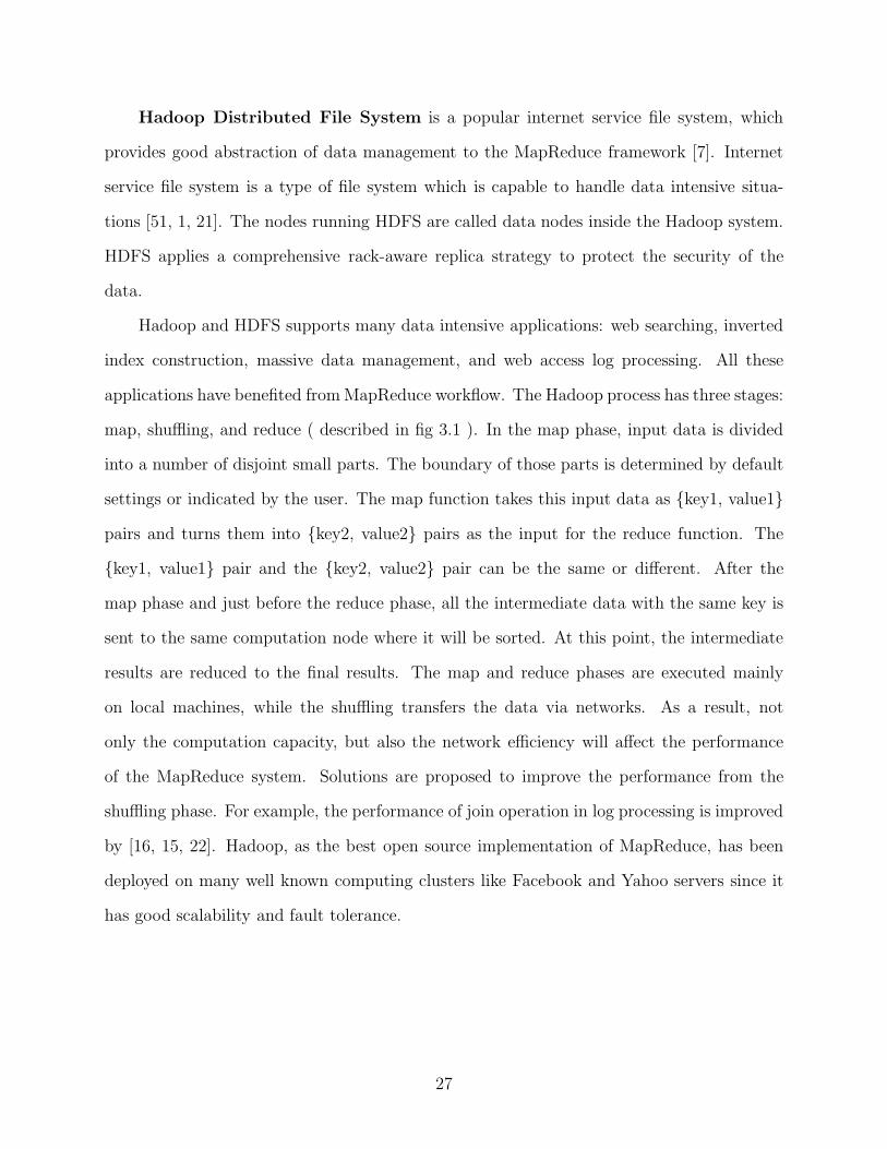
Hadoop Distributed File System is a popular internet service file system, which

provides good abstraction of data management to the MapReduce framework [7]. Internet

service file system is a type of file system which is capable to handle data intensive situa-

tions [51, 1, 21]. The nodes running HDFS are called data nodes inside the Hadoop system.

HDFS applies a comprehensive rack-aware replica strategy to protect the security of the

data.

Hadoop and HDFS supports many data intensive applications: web searching, inverted

index construction, massive data management, and web access log processing. All these

applications have benefited fromMapReduce workflow. The Hadoop process has three stages:

map, shuffling, and reduce ( described in fig 3.1 ). In the map phase, input data is divided

into a number of disjoint small parts. The boundary of those parts is determined by default

settings or indicated by the user. The map function takes this input data as {key1, value1}

pairs and turns them into {key2, value2} pairs as the input for the reduce function. The

{key1, value1} pair and the {key2, value2} pair can be the same or different. After the

map phase and just before the reduce phase, all the intermediate data with the same key is

sent to the same computation node where it will be sorted. At this point, the intermediate

results are reduced to the final results. The map and reduce phases are executed mainly

on local machines, while the shuffling transfers the data via networks. As a result, not

only the computation capacity, but also the network efficiency will affect the performance

of the MapReduce system. Solutions are proposed to improve the performance from the

shuffling phase. For example, the performance of join operation in log processing is improved

by [16, 15, 22]. Hadoop, as the best open source implementation of MapReduce, has been

deployed on many well known computing clusters like Facebook and Yahoo servers since it

has good scalability and fault tolerance.

27

3.3 Performance Analysis of Hadoop Clusters

In order to demonstrate the performance issues in Hadoop clusters, we test the Hadoop

system using various experimental settings. By analyzing performance results collected from

a wide range of experiments, we are able to identify the flaws and bottlenecks lies in tradi-

tional Hadoop systems.

3.3.1 Experimental Setup

We perform experiments in two computing environments - a standalone (i.e., single

node) Hadoop and a multiple-node Hadoop cluster. Table 3.3.1 shows the configurations of

all the computing nodes involved in the our experiments.

Computing Node CPU Memory DiskNode1 Duo-Core 3.0GHz 4G NANode2 Quad-Core 2G NANode3 Quad-Core 2G NANode4 Quad-Core 2G NA

Table 3.1: Computing Nodes Configurations

3.3.2 Performance Impacts of Small Blocks

The focus of the first experiment is to evaluate the impact of small blocks on the

performance of the WordCount application running in the single-node Hadoop system. We

set the block size to 64MB, 128MB, and 256MB, respectively. The input file size is 1GB.

X-axis and Y-axis in Figures 3.2-3.4 represent running time and CPU utilization. A general

observation drawn from the experimental results is that increasing block size noticeably

improves system performance. For example, in the worst case where the block size is as

small as 1MB, the execution time of WordCount is over 2500 seconds. When the block size

is 64MB, it takes the Hadoop system 225 seconds to complete WordCount (see Figure 3.2).

If the block is increased to 256MB, the execution time of WordCount is shorten down to

28

0

10

20

30

40

50

60

70

80

90

0 50 100 150 200 250

%user

Time (in seconds)

Hadoop Wordcount - 1GB file (64MB block size)

Figure 3.2: CPU utilization for wordcount with block size 64MB

205 seconds (see Figure 3.4. We attribute this reduction in execution time to the I/O

improvement, which is illustrated as follows.

Figures 3.2-3.4 show that when the Hadoop system finishes processing a block, the

CPU utilization drops significantly. The CPU utilization periodically slides, because the

CPU must wait a subsequent block to be loaded from the disk. When block size is 64MB

and 128MB, the CPU utilization drops eight and four times, respectively. If we increase

block size up to 256MB, the CPU utilization only periodically drops twice. A large block

size helps to reduce I/O processing time by decreasing the number of I/O accesses. As a

result, the I/O waiting time between two continuous small blocks (see Figure 3.2) is longer

than that of two continuous large blocks (see Figure 3.4).

The above experimental results show that small files have a huge impact on the Hadoop

system. In general, there are the following three approaches to solving the problem caused

by small files.

• Hadoop Archive (HAR). An HAR package compresses multiple small files into a single

large file. Unlike traditional compressed files, each small file in the HAR package can

be directly accessed thanks to an index of the small files maintained by HAR.

29

0

10

20

30

40

50

60

70

80

90

0 50 100 150 200 250

%user

Time (in seconds)



0

10

20

30

40

50

60

70

80

90

100

0 50 100 150 200 250

%user

Time (in seconds)



30

• Combine File Input Format. It is also known as CombineFileInputFormat, which is

implemented as one of the Hadoop’s application programming interfaces (APIs) [50].

The CombineFileInputFormat interface combines small files to form a block in a given

size.

• Sequence File. A sequence file is a flat file that contains binary key value pairs. Hadoop

intermediate results generated during the map phase are collected using this file format.

The above three solutions have some drawbacks. For example, there is no efficient way

to modify HAR files after they are created. If an HAR file is updated, the HAR file must

be recreated from ground up, which is a time consuming process when the HAR file is large.

The combined file input format and sequence file format offered as APIs of Hadoop require

application developers to write specific code to handle small files. If programmers decide to

take the last two approaches to deal with small files, the programmers have to first identify

small files manually and then apply the APIs to handle the small files. Alternatively, the

programmers may write code to automatically identify small files.

In our future study, we plan to design a mechanism to dynamically modify small files

packed inside an HAR file. The goal of this mechanism is to update small files without

recreating the entire HAR file.

3.3.3 Performance Impacts of Network Interconnects

The goal of our proposed KAT is to address the network performance issue raised in the

shuffling phase. We expect that KAT will perform very well if network interconnects become

a performance bottleneck in Hadoop clusters. Before we design and implement KAT, we

illustrate that network interconnects have noticeable impacts on the performance of HDFS,

which relies on high-speed networks for fast data transfers.

There are two general approaches to addressing network problems in Hadoop clusters.

The first approach is to increase the bandwidth of network interconnections; the second one

31

!"

#!"

$!!"

$#!"

%!!"

%#!"

&!!"

&#!"

'!!"

'#!"

%"()*+," '"()*+," -"()*+,"

!"#$%"&'()*+%&,"')-./0)

.)/*0)1(2"34015)("678+"

.)/*0)1(2"34015)("678+"

7(".)/,+"9+2:)/;"

Figure 3.5: Execution times of WordCount under good and poor network conditions; timesare measured in Second.

is to reduce the amount of data being transferred among data nodes. We show below that

network performance affects the execution time of Hadoop applications; we also show that

poor network performance may increase the amount of transferred data. More specifically,

we conduct two experiments to quantitatively show the impact of networks on the execution

times of a Hadoop application (i.e., WordCount) and the amount of data transferred among

the data nodes in a Hadoop cluster.

Although network interconnects in modern Hadoop clusters offer high I/O bandwidth,

observed network bandwidth from the perspective of a single application might be poor

due to resource sharing. Low observed network bandwidth is not uncommon in a cluster

computing environment, where each node is running multiple virtual machines sharing the

bandwidth.

To study the impact of observed network bandwidth available to the tested Hadoop

application, we apply the traffic shaping technique to manipulate observed network band-

width. For example, traffic shaping can significantly reduce each node’s bandwidth allocated

to the map and reduce phases of the WordCount application. We employ the ”TC” utility

32

!"

!#$"

%"

%#$"

&"

&#$"

'"

'#$"

("

&")*+,-" (")*+,-" .")*+,-"

!"#$%"&'()*#+,%)-".&/0)

/*0+1*2)3"40561"

7*829,"

/*0+1*2)3"40561"

7*829,":)"/*0-,"

;,3<*0="

Figure 3.6: Amount of data transferred among data nodes running WordCount under goodand poor network conditions; data size is measured in GB.

program to record an initial data usage on each node as well as data usage on the same node

after WordCount is completed. An entire data usage during the execution of WordCount is

calculated by aggregating all the nodes’ data usage.

In our experiments, the bandwidth is limited to 500Mbps to resemble real-world cases

where two virtual machines are sharing the 1Gbps network. Figure 3.5 shows the response

time of WordCount on the Hadoop cluster. We observe that when the observed network

bandwidth is reduced from 1Gpbs down to 500Mbps, the WordCount’s response time is

increased by 12%. Comparing the 2-node, 4-node, and 8-node Hadoop clusters, we discover

that poor network bandwidth have more negative impacts on the 8-node cluster than on the

2-node cluster. This performance trend implies that when observed network bandwidth is

degraded in a large-scale cluster, Hadoop applications will experience noticeably increased

execution times.

To investigate the reason behind the negative impacts of degraded network intercon-

nects, we measure the amount of transferred data among the nodes running WordCount

under good and poor network conditions. Figure 3.6 shows that the transferred data volume

33

is increased significantly when the bandwidth is shared among multiple virtual machines.

More importantly, Figure 3.6 indicates that when the number of data nodes goes up from 2

to 8, the transferred data volume is increased by a factor of 5 and 3.8 under good and poor

network conditions.

We conclude from the above experimental results that network traffic can inevitably

affect the performance of Hadoop clusters. The preliminary results motivate us to address

the performance problem induced by the increased amount of transferred data among nodes.

In particular, we design the KAT scheme to reduce the amount of transferred data by pre-

calculating intermediate keys according to which input files are placed. KAT can alleviate the

network performance bottleneck problem imposed by data transfers, because data sharing

the same key are not scattered across nodes of a cluster.

3.4 Key-Aware Data Placement

KAT is a key-aware data placement strategy that addresses the data transfer overheads

in the shuffling phase of Hadoop applications. In this section, we discuss challenges and

design issues of developing KAT in HDFS.

3.4.1 Design Goals

We design KAT that can be implemented as a module incorporated into Hadoop’s

HDFS. When HDFS places files on data nodes, HDFS does not take into account the at-

tributes (i.e., keys and values) of input files. HDFS indiscriminately considers all the input

data entries during the data distribution process. Although the benefit of this strategy is

to well balance load across nodes in a Hadoop cluster, it can lead to a large amount of

transferred data during the shuffling stage of Hadoop. To address this problem, we propose

KAT - an intermediate key-aware distribution strategy - to allocate data according to pre-

calculated intermediate key values. In other words, data sets are distributed based on their

34

intermediate keys; the data distribution module is aware of data locations. The data distri-

bution is predictable and controlled by KAT. System administrators, of course, can change

the configurations of KAT according to cluster settings to optimize system performance.

The KAT strategy is implemented at both the application and system level. Since in-

termediate keys may have various values in different applications, we must facilitate each

application with a pre-calculation module. Given a Hadoop application, the Hadoop run-

time system has to be updated to maintain information regarding the pre-calculations of

intermediate keys. During the data distribution process, a hash function is used to decide

target data nodes to which data entries are allocated.

Our KAT strategy aims to improve the performance of Hadoop applications by reducing

network transmission overhead. Data transfer times are shortened during the shuffling stage.

Moreover, performance stability can be improved by KAT thanks to the fact that data allo-

cations are predictable. When using the data placement strategy in the native Hadoop, the

namenode randomly picks a data node for input data. Such a random datanode selection

process may cause two problems. First, data placement might be unbalanced in a Hadoop

cluster due to random datanode selections. In the worst case, all the data may be placed

in a single data node, which becomes a performance bottleneck causing network commu-

nications. Second, randomly selected data data nodes make data placement unpredictable.

Consequently, network communications are unpredictable, thereby making it difficult to con-

trol the performance of Hadoop in a certain range. There is a big difference between the

best data placement decision and the worst one; there is no guarantee that random data

placement delivers the best performance every time. In our solution, data allocations are

judiciously managed by the KAT data-placement strategy. Data placement decisions made

by KAT allow each Hadoop application to exhibit stable performance.

35

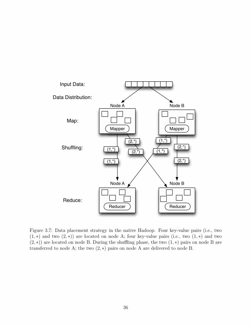
Input Data:

Mapper

Node A

Mapper

Node B

Data Distribution:

Map:

Shuffling:

Reduce:Reducer

Node A

Reducer

Node B

(1,*)

(1,*)

(1,*)

(1,*)

(2,*)

(2,*)(2,*)

(2,*)

Figure 3.7: Data placement strategy in the native Hadoop. Four key-value pairs (i.e., two(1, ∗) and two (2, ∗)) are located on node A; four key-value pairs (i.e., two (1, ∗) and two(2, ∗)) are located on node B. During the shuffling phase, the two (1, ∗) pairs on node B aretransferred to node A; the two (2, ∗) pairs on node A are delivered to node B.

36

Input Data:

Mapper

Node A

Mapper

Node B

Data Distribution:

Map:

Shuffling:

Reduce:Reducer

Node A

Reducer

Node B

(1,*)

(1,*)

(1,*)

(1,*)(2,*)

(2,*)

(2,*)

(2,*)

(2,*)

(2,*)

(2,*)

(2,*)

(1,*)

(1,*)

(1,*)

(1,*)

pre-key-calculator

Figure 3.8: KAT: a key-based data placement strategy in Hadoop. KAT assigns the four(1, ∗) key-value pairs to node A and assigns the four (2, ∗) key-value pairs to node B. Thisdata-placement decision eliminates the network communication overhead incurred in theshuffling phase.

37

3.4.2 The Native Hadoop Strategy

Before presenting the design of KAT, let us briefly describe the data-placement strat-

egy implemented in the native HDFS. To simplify the description, we show how data are

distributed in HDFS in the single-data-replica case, where each data set has one copy in

HDFS.

In native HDFS, data files are written into a disk through a buffer. When the buffer

is filled up with files or there is no more incoming data to the buffer, a waiting process is

triggered to pack the buffered data together and delivers the packed data to a list of target

data nodes. If files only have one local copy without any remote replica, the list of data

nodes is empty. After a data node receives the packed data, the node needs to deal with two

issues. First, the node checks the list of data nodes embedded in the package. If the list is

not empty (i.e., data have remote replicas), the data node will forward the data package to

the first node in the list. Second, the node writes the content of the package into the node’s

disk.

This native data-placement strategy may lead to a potential performance problem -

data with the same keys might be allocated to different data nodes, causing unnecessary

data transfer overheads. Figure 3.7 uses an example to illustrate the above performance

problem. In this example, four key-value pairs (i.e., two (1, ∗) and two (2, ∗)) are located on

node A; similar four key-value pairs (i.e., two (1, ∗) and two (2, ∗)) are located on node B.

During the shuffling phase, the two (1, ∗) key-value pairs residing in node B are transferred

to node A; the two (2, ∗) key-value pairs on node A are delivered to node B.

To address the aforementioned problem, our KAT strategy assigns the four (1, ∗) key-

value pairs to node A and assigns the four (2, ∗) pairs to node B. Figure 3.8 illustrates that

the data-placement decision made by KAT eliminates the network communication overhead

incurred in the shuffling phase.

Now we describe how the data-placement strategy in HDFS chooses target data nodes

when data nodes of a Hadoop cluster are located in multiple racks. Let us consider a

38

case where three different data nodes must be chosen to store data, the strategy in the

native HDFS guarantees that two data nodes are located within one rack while the third

node is residing in another rack. This random-selection scheme is normally employed until

unbalanced data volume reaches a specified threshold. Once the threshold is reached, a

balancing process is activated to reallocate data in a way to balance load among the data

nodes.

3.4.3 Implementation Issues

The Pre-Calculation Module

There are two approaches to reducing network communication overheads in Hadoop

clusters. The first one is to reduce the amount of transferred intermediate data; the second

one is to minimize the size of communication data including data migrated during the load

balancing process. This study is focused on the first approach because of the following

two reasons. First, the amount of migrated data is not as huge as that of transferred

intermediate data. Second, most of the network overhead introduced by migrated data

can not be eliminated. As such, we intend to take the first approach to reducing network

overhead by decreasing the amount of transferred intermediate data.

To reduce the amount of transferred intermediate data, we implement a pre-calculation

module and a data distribution module (see Section 3.4.3). The pre-calculation module (see

Figure 3.8) is responsible for pre-calculating intermediate keys for data entries; the data

distribution module is in charge of allocating data according to the pre-calculated keys. The

pre-calculation module performs in combination with the data distribution module to ensure

that data with the same intermediate key value are placed on the same data node.

The Data Distribution Module

Recall that the data distribution module aims to distribute data entries coupled with

pre-calculated key values to data nodes. In this distribution module, we implement a hash

39

function to map input data keys onto a set of data nodes. Note that the number of data

nodes in our testbed is eight. Input data are evenly distributed to all the available data

nodes. In the best case, all the data nodes complete their map phase at approximately the

same time.

Because of the evenly distributed data processed by the data distribution module in

KAT, a huge amount of migrated data can be avoided in the load balancing process. In

some cases, our hash function in the distribution module can be incorporated with the load

balancing module in the Hadoop runtime system to further improve system performance.

Figure 3.8 shows that thanks to the KAT strategy, key-value pairs with the same key no

long need to be transferred among multiple data nodes after the map phase.

Data Redistribution Module

Now we discuss the implementation issues related to the above two KAT modules. There

two cases in which which the KAT modules are invoked to pre-calculate keys and distribute

files to data nodes in a Hadoop cluster. In the first case, data files are imported into the

HDFS file system. In the second case, updated data files must be redistributed for the

purpose of load balancing.

The first case can be addressed by replacing the current data distribution module in

HDFS with our KAT modules. This approach is inexpensive in terms of computing and

data transfer overheads. The downside of this approach is that the second case can not be

covered. Nevertheless, another data redistribution module must be implemented to handle

the second case. The data redistribution module is implemented in a similar way as that of

the data distribution module in KAT.

Apart from the aforementioned approach, another candidate solution is to trigger the

data redistribution module when a data modification process is finished. This solution

addresses the above two cases. Compared with the first approach, the second solution takes

longer time periods to import files into HDFS for the first time. In the worst case, the second

40

approach needs to relocate all the data imported for the first time. Our goal is to investigate

performance improvement offered by the KAT data-placement strategy and; therefore, we

choose the first approach and implement the data redistribution module coupled with the

two KAT modules.

System-Level Implementation

The two KAT modules along with the data redistribution module can be implemented

at either the application level or the Hadoop system level. Although implementing KAT at

the application level is easy, this approach is not transparent to Hadoop applications. In our

implementation, we add the two KAT modules in the Hadoop system.

The first module is in charge of pre-calculating intermediate keys. This module obtains

intermediate key values from input entries. Hadoop applications offer hints regarding in-

termediate keys to the pre-calculation module in KAT; the hints allow the pre-calculation

module to compute key values prior to the executions of the applications.

The second module is responsible for distributing data to nodes in a Hadoop cluster.

The native module in HDFS (see Figure 3.9) maintains one queue on namenode to manage

data blocks with a fixed size. In our implementation, we extend this existing module so that

data blocks located in the single queue can be delivered to multiple data nodes. There are

the following two ways of extending the module in the native HDFS.

First, we implement multiple queues in the namenode. Each queue is dedicated to

a data node. Data blocks are dispatched to different queues according to hashing results

of intermediate keys. Although this solution is straightforward, it might not be a feasible

solution for large-scale Hadoop clusters where a large number of queues must be maintained

by the namenode.

Second, we implement distributed queues located in all data nodes. In this imple-

mentation, each data entry is examined by the pre-calculation module and is mapped to

a corresponding data node using the hash function. Then, the data entry is sent to the

41

Figure 3.9: The architecture of a Hadoop cluster [34]. The data distribution module inHDFS maintains one queue on namenode to manage data blocks with a fixed size.

42

data node where the local queue is used to manage the data. When the local queue is full,

data stored in the queue are packed to a single data block, which is imported to the local

HDFS space. The drawbacks of this implementation is that separately delivering data entries

inevitably increases network transfer overheads.

When it comes to small-scale Hadoop clusters, the first approach (i.e., centralized queue

in the namenode) is better than the second one (i.e., distributed queues in all data nodes).

In contrast, the second implementation is better than the first one when KAT is applied to

solve the data distribution problem in large-scale Hadoop clusters.

Application-Level Implementation

Implementing KAT at the system level of Hadoop makes KAT transparent to appli-

cations. The system-level implementation has two drawbacks. First, system-level imple-

mentation is more complicated than the application-level counterpart. Second, we have

to implement an application programming interface (API) allowing applications to provide

application-specific algorithms to calculate intermediate keys at the system level. To over-

come the above shortcomings, one may implement KAT at the application level.

Given input files and a Hadoop application, the system-level KAT and application-

level KAT achieve makes the same data-placement decisions. We can use the system-level

implementation to validate the correctness of the application-level implementation, and vice

versa. We implement the KAT module at the application level to distribute data for two

real-world Hadoop applications (i.e., WordCount and Grep). We also use input files of 500

MB to validate the correctness of the KAT modules supporting the WordCount and Grep

applications.

3.5 Experimental Results

In this section, we use two real-world Hadoop applications - WordCount and Grep - to

evaluate the performance of our proposed KAT strategy. We also compare KAT with the

43

data-placement strategy implemented in the native Hadoop system. The size of input files

for the two Hadoop applications is 8 GB. We set the number of data nodes in a Hadoop

cluster to 2, 4, and 8.

3.5.1 Experimental Setup

We implement KAT and evaluate it on a 9-node Hadoop cluster, which consists of a

name node and eight data nodes connected with a 1 Gbps Ethernet switch. Table 3.2 shows

the configuration of the nodes in the tested Hadoop cluster. The name node (see Figure 3.9)

is responsible for assigning jobs and managing the data nodes; there is no map or reduce

task running on this name node. Data are stored on the eight data nodes, on which map

and reduce tasks are running. All the data nodes’ names are listed in a configuration file on

the name node. We change the number of data nodes in the Hadoop cluster by updating

the configuration file for the data-node list.

Two important performance metrics measured in our experiments are execution time

and the amount of transferred data. Execution times are measured in second; data amount

is measured in GByte. To evaluate the scalability of our KAT strategy, we vary the number

of data nodes in the tested cluster (see Section 3.5.2). Using the 2-node, 4-node, and 8-

node Hadoop clusters, we show KAT’s impact on network traffic of the Hadoop system

(see Section 3.5.3). In addition to cluster size, block size and fie size are evaluated in our

experiments (see Section 3.5.4). The analysis of KAT’s stability and Map/Reduce processes

can be found in Sections 3.5.5 and 3.5.6, respectively.

We run two Hadoop applications (i.e., WordCount and Grep) on the cluster. WordCount

- a basic application for web search indexing - is an application that counts words in input

files. Grep counts the number of matches of a given input expression. The total size of

all the input files is 8 GB. Average file size is 500 MB for all the experiments. Each file is

partitioned into two equal sized blocks of 256MB according to the configuration file’s settings.

The number of map tasks is set to four for each data node, because the data nodes in the

44

Table 3.2: Configurations of name and data nodes in the Hadoop cluster.Type Hardware Software

1×Intel Xeon 2.4 GHz processor Ubuntu10.04

Name 1×4 GBytes of RAM Linux kernel2.6.23

Node 1×1 GigaBit Ethernet networkcard

Hadoop0.20.2

×1 1×Seagate 160 GBytes Sata disk(ST3160318AS)Intel Xeon 2.4 GHz processor Ubuntu

10.04Data 2 GBytes of RAM Linux kernel

2.6.23Node 1 GigaBit Ethernet network card Hadoop

0.20.2×8 1×Seagate 160 GBytes Sata disk

(ST3160318AS)

tested cluster are equipped with quad-core processors. Four map tasks can fully utilize the

quad-core processors in the Hadoop cluster. Similarly, the number of reduce tasks is limited

to up to 4 per node.

During the entire evaluation process, we conduct hundreds of tests and record all the

test outputs as text files. The output text files indicate that the number of reducers never

reaches the limit regardless of the number of data nodes. In each experiment, we run the

Hadoop benchmark for ten times and report the average of the ten measures.

3.5.2 Scalability

Now we evaluate the impact of the number of data nodes on the performance of KAT.

We test both the native Hadoop system and the KAT-enabled system on 2-node, 4-node,

and 8-node clusters, respectively. The observed network bandwidth is manipulated by the

the bandwidth control technique described in Section 3.3.

Figure 3.10 shows the execution times of WordCount and Grep running in the tested

cluster where the number of data nodes is set to 2, 4, and 8, respectively. The results show

that when the network bandwidth is 1 Gbps, KAT reduces the execution times of both

WordCount and Grep, regardless of the number of data nodes in the cluster. Comparing

45

!"#$%&

'(!$'&

))"$*&

*#)$!&

'(($*&

))+$)&

+*'$"&

%+($(&

(#,"$+&

*'%$"&

'(!$!&

),+$,&

#&

)##&

'##&

%##&

*##&

(###&

()##&

)& '& *&

!"#$%&'()*+,

#)-./)

0%,1#2)'3)4565('7#8)

-./01&2.3445&.6&(7859&

:;<&1=.8>13&.6&(7859&

-./01&2.3445&.6&(#?859&

:;<&1=.8>13&.6&(#?859&

(a) Wordcount execution time in 1Gbps network

!"#$!%

&'#$'%

(($)%

!&!$*%

&!)$(%

+'$+%

!&!$(%

*#)$*%

+",$,%

!&,$,%

&!+$)%

++$,%

#%

&##%

!##%

"##%

*##%

)##%

'##%

,##%

+##%

(##%

!% *% +%

!"#$%&'()*+,

#)-./)

0%,1#2)'3)4565('7#8)

-./01%2.3445%.6%&7859%

:;<%1=.8>13%.6%&7859%

-./01%2.3445%.6%&#?859%

:;<%1=.8>13%.6%&#?859%

(b) Grep execution time in 1Gbps network

Figure 3.10: Execution Times of Grep and Wordcount on the Hadoop cluster. The numberof data nodes is set to 2, 4, and 8, respectively.

46

the two Hadoop applications, we observe that Grep gains more benefits from KAT than

WordCount does. This trend is reasonable because Grep exchanges more intermediate data

during the shuffle phase than WordCount, meaning that Grep offers more opportunities for

KAT to improve system performance.

Figure 3.10 also reveals that compared with the native Hadoop system, our KAT is

less sensitive to the number of data nodes in the cluster. This trend suggests that KAT is

much more scalable than the native Hadoop system. When the observed network bandwidth

drops down to 10Mbps, KAT significantly improves the performance over the native Hadoop

system. These results indicates that KAT performs extremely well when observed network

bandwidth of Hadoop cluster is very low.

3.5.3 Network Traffic

Recall that KAT improves the performance of the native Hadoop system by reducing

network traffic. In this group of experiment, we show evidence that KAT can alleviate

network traffic burden of Hadoop clusters running WordCount and Grep.

The three Hadoop clusters used in this experiment are the same as those described in

Section 3.5.2. Before running the Hadoop benchmark, we record the total network usage

measured in GByte. Upon the completion of the test, we record the total network usage

on each data node. Then, we derive the network usages by subtracting the network usages

measured before the test from the one measured after the test.

Figure 3.11 shows that the network usage increases when the Hadoop cluster scales

up; the average network transmission rate is getting higher when the number of data nodes

increases. Nevertheless, the observed network bandwidth will reach the system’s maximum

bandwidth when the number of nodes continues going up.

Although KAT only slightly improves the performance of the two applications when the

network bandwidth is 1Gbps, Figure 3.11 indicates that KAT noticeably reduces network

47

!"#$

!"#%

!"#&

!"#$ '()*+(,-.

!"!!/

!"0!/

1"!!/

1"0!/

2"!!/

2"0!/

&"!!/

&"0!/

2-(*34/ #-(*34/ %-(*34/

!"#$

%&'()&*+,(-./01(

!230"&(%4(5*#*6%7"8(

56783/19:;4/

<=>/19:;4/

56783/1!?:;4/

<=>/1!?:;4/

(a) Wordcount traffic in 1Gbps network!"#$%$&'()&*

+,-. /0'1

2,+3

4,.5

.,2.

+,67

4,-3

.,22

.,67

.,.4

.,.-

.,.-

.,.7

+,44

6,75

6,68

.,5-

+,46

2,.2

.,72

.,-.

.,..(

.,7.(

+,..(

+,7.(

6,..(

6,7.(

2,..(

2,7.(

4,..(

4,7.(

7,..(

69":'#( 49":'#( 89":'#(

!"#$

%&'()&*+,(-./01(

!230"&(%4(5*#*6%7"8(

;<=&'(+/>1#(

?)@(+/>1#(

;<=&'(+.A>1#(

?)@(+.A>1#(

(b) Grep traffic in 1Gbps network

Figure 3.11: Network traffics of the Wordcount and Grep Applications.

48

!"!#

$!"!#

%!"!#

&!"!#

'!"!#

(!"!#

)!"!#

*!"!#

+!"!#

)'# $%+# %()#

!"#

$%&'(%

)*+,-%'".$%&/)(%

,-./0#1-2334#

567#08-9:02#

Figure 3.12: Grep with 2GB input in 1Gbps network

traffic for the two Hadoop applications. In terms of network-traffic reduction, KAT has more

significant impacts on Grep than on WordCount.

KAT conserves network bandwidth for network-intensive applications sharing network

resources with Hadoop applications on clusters. Our results confirm that when most of

the network bandwidth is reserved for other network-intensive applications, KAT works

particularly well in terms of reducing network traffic of Hadoop applications that experience

slow observed network bandwidth.

3.5.4 Block Size and Input Files Size

In this group of experiments, we evaluate the impact of block size and total input-file

size on the performance of KAT. The block size can be modified in the configuration file.

The block size is chosen to be 64MB, 128MB, and 256MB, respectively; we set the total

input data size to 8GB, 4GB, and 2GB, respectively.

Figure 3.12 - 3.23 shows that when the total input file size is 2GB, decreasing block

size allows KAT to achieve better performance. When the total input file is 4GB, however,

the advantage of small blocks becomes diminished. Interestingly, when the total input file

49

!"!#

$!"!#

%!"!#

&!"!#

'!"!#

(!"!#

)!"!#

*!"!#

+!"!#

,!"!#

)'# $%+# %()#

!"#

$%&'(%

)*+,-%'".$%&/)(%

-./01#2.3445#

678#19.:;13#


!"!#

$!"!#

%!"!#

&!"!#

'!"!#

(!!"!#

($!"!#

&%# ($'# $)&#

!"#

$%&'(%

)*+,-%'".$%&/)(%

*+,-.#/+0112#

345#.6+78.0#


50

!"!#

$!!"!#

%!!"!#

&!!"!#

'!!"!#

(!!"!#

)!!"!#

)'# $%*# %()#

!"#

$%&'(%

)*+,-%'".$%&/)(%

+,-./#0,1223#

456#/7,89/1#

Figure 3.15: Grep with 2GB input in 10Mbps network

!"!#

$!!"!#

%!!"!#

&!!"!#

'!!"!#

(!!"!#

)!!"!#

)'# $%*# %()#

!"#

$%&'(%

)*+,-%'".$%&/)(%

+,-./#0,1223#

456#/7,89/1#


51

!"!#

$!!"!#

%!!"!#

&!!"!#

'!!"!#

(!!"!#

)!!"!#

*!!"!#

+!!"!#

,!!"!#

)'# $%+# %()#

!"#

$%&'(%

)*+,-%'".$%&/)(%

-./01#2.3445#

678#19.:;13#


!"!#

$!"!#

%!"!#

&!"!#

'!"!#

(!!"!#

($!"!#

(%!"!#

(&!"!#

('!"!#

&%# ($'# $)&#

!"#

$%&'(%

)*+,-%'".$%&/)(%

*+,-.#/+0112#

345#.6+78.0#

Figure 3.18: Wordcount with 2GB input in 1Gbps network

52

!

"#"$

%"#"$

&"#"$

'"#"$

("#"$

)""#"$

)%"#"$

)&"#"$

)'"#"$

)("#"$

%""#"$

'&$ )%($ %*'$

!"#

$%&'(%

)*+,-%'".$%&/)(%

+,-./$0,122!$

345$/6,78/1$


!"!#

$!"!#

%!!"!#

%$!"!#

&!!"!#

&$!"!#

'(# %&)# &$'#

!"#

$%&'(%

)*+,-%'".$%&/)(%

*+,-.#/+0112#

345#.6+78.0#


53

!"!#

$!"!#

%!!"!#

%$!"!#

&!!"!#

&$!"!#

'!!"!#

'$!"!#

(!!"!#

($!"!#

)(# %&*# &$)#

!"#

$%&'(%

)*+,-%'".$%&/)(%

+,-./#0,1223#

456#/7,89/1#

Figure 3.21: Wordcount with 2GB input in 10Mbps network

!"!#

$!!"!#

%!!"!#

&!!"!#

'!!"!#

(!!"!#

)!!"!#

*!!"!#

+!!"!#

)'# $%+# %()#

!"#

$%&'(%

)*+,-%'".$%&/)(%

,-./0#1-2334#

567#08-9:02#


54

!"!#

$!!"!#

%!!"!#

&!!"!#

'!!"!#

(!!!"!#

($!!"!#

&%# ($'# $)&#

!"#

$%&'(%

)*+,-%'".$%&/)(%

*+,-.#/+0112#

345#.6+78.0#


size is 8 GB, large blocks are better than small blocks in terms of performance improvement

offered by KAT.

Figs. 3.18-3.20 shows that the native Hadoop system is very sensitive to observed net-

work bandwidth. For example, the execution times of Hadoop applications are increased by

an factor of 8 when the network bandwidth is reduced from 1Gbps to 10Mbps. The bigger

the block size, the slower the performance of the native Hadoop system. In contrast, the

KAT-enabled cluster is not very sensitive to the observed network bandwidth, because KAT

substantially reduces transferred data amount. When it comes to KAT, 256MB block size

leads to better performance than the block size of 64MB for both benchmarks when the

input data set is large (e.g., 2-8 GB).

3.5.5 Stability of KAT

This group of experiments is focused on the stability of KAT. A high stability means that

KAT achieves similar performance for different experiments as long as the Hadoop computing

environment remains unchanged. To show evidence that KAT is more stable than the native

Hadoop system, we run each test 10 times and calculate the standard deviation.

55

!"

#"

$"

%"

&"

'"

("

)"

*"

$" &" *"

!"#$%#&%'()*+#,-$'

!+.)'-/'0$12"'3+4)5'6789'

+,-./(&01"

+,-./#$*01"

+,-./$'(01"

234(&01"

234#$*01"

234$'(01"

Figure 3.24: Standard deviation of Grep in 1Gbps network

!"#$%

!"&#%

'"!(%

!")&%

!"&*%

$")'%

+"#'%

!"&!%

#"(!%

!%

(!%

+!!%

+(!%

$!!%

$(!%

$% #% ,%

!"#$%#&%'()*+#,-$'

!+.)'-/'0$12"'3+4)5'6789'

-./01)#23%

-./01+$,23%

-./01$()23%

456)#23%

456+$,23%

456$()23%

Figure 3.25: Standard deviation of Grep in 10Mbps network

56

!"

#"

$"

%"

&"

'!"

'#"

'$"

#" $" &"

!"#$%#&%'()*+#,-$'

!+.)'-/'0$12"'3+4)5'6789'

()*+,%$-."

()*+,'#&-."

()*+,#/%-."

012%$-."

012'#&-."

012#/%-."

Figure 3.26: Standard deviation of Wordcount in 1Gbps network

!"#$%

$"&$%

#"''%

("$'%

)"('%

!*")#%

'"&!%

)"*(%

+"(*%

*%

'**%

#**%

+**%

(**%

!***%

'% #% (%

!"#$%#&%'()*+#,-$'

!+.)'-/'0$12"'3+4)5'6789'

,-./0+#12%

,-./0!'(12%

,-./0'&+12%

345+#12%

345!'(12%

345'&+12%

Figure 3.27: Standard deviation of Wordcount in 10Mbps network

57

Figure 3.24 reveals that when the network bandwidth is 1 Gbps, the standard deviation

of Grep using the native Hadoop goes up with the increasing block size. When the total

input file size is increased from 2GB to 8GB, the deviation of the native Hadoop system

noticeably increases. Unlike the native Hadoop, KAT’s standard deviation is non-sensitive

to the total input size and block size.

Figure 3.25 shows the standard deviations when the observed network bandwidth is

10Mbps. The results plotted in Figure 3.25 reveals that a low network bandwidth leads

to a large standard deviation for the native Hadoop, the performance of which is unstable.

Fortunately, even in case of a low network bandwidth, the performance of KAT is still

very stable. Moreover, KAT’s stability is not dramatically affected by network conditions.

The performance deviations of the native Hadoop share the same trend as that shown in

Figure 3.24. The native Hadoop’s performance deviation increases along with both input

size and block size. The experimental results indicate that in the native Hadoop system,

small block sizes or input data set help applications to achieve stable performance.

Figure 3.26 shows that the standard deviation of WordCount is larger than that of Grep

in both the native Hadoop and KAT when the network bandwidth is 1Gbps. In some cases,

KAT and the native Hadoop share very similar standard deviations. Furthermore, when

the input size equals to 2GB, KAT has higher deviation than that of the native Hadoop.

Nevertheless, the stability of KAT remains unchanged when the input size increases; the

native Hadoop has higher performance deviations whein the input data set becomes larger.

We conclude from this group of experiments that KAT is expected to outperform the native

Hadoop when input data sets scale up.

Figure 3.27 indicates that in case of low network bandwidth, WordCount’s standard

deviation in the native Hadoop increases when the block size or total file size are increased.

The results also show that the stand deviation of WordCount supported by KAT is very

small, meaning that KAT offer very stable performance for WordCount. The results plotted

in Figure 3.27 are consistent with those in Figure 3.25.

58

!"#

$!"#

%!"#

&!"#

'!"#

(!"#

)!"#

*!"#

+!"#

,!"#

$!!"#

!#

%$#

%,#

&+#

')#

('#

)&#

*$#

+!#

++#

,)#

$!(#

$$&#

$%%#

$&$#

$&,#

$'*#

$()#

$)'#

$*'#

$+,#

%!!#

%%!#

!"#$"%&&'

()*%'+,%-#./&0'

-./#

012341#

Figure 3.28: Wordcount Execution process of Traditional Hadoop with 1Gbit/s Bandwidth

In summary, Figures 3.24-3.27 show clear evidence that the native Hadoop’s stability

is substantially affected by block size and input file size. Small block and input data sizes

tend to give rise to more stable performance in the native Hadoop system. In addition

to block and input data sizes, network bandwidth can seriously affect the native Hadoop’s

performance stability. High network bandwidth gains better performance stability for the

native Hadoop. Unlike the native Hadoop, KAT’s performance stability is independent of

network bandwidth.

3.5.6 Analysis of Map and Reduce Processes

Now we take a close look at map and reduce tasks when KAT is applied to improve the

system performance of Hadoop. We play a particular attention to the shuffling phase of the

application supported by KAT and the native Hadoop. In this group of experiments, the

total input file size is 8GB, block size is 256MB, and the number of data nodes is 8.

Figure 3.28 shows that when the observed network bandwidth is 1Gbps, the native

Hadoop finishes task within 227 Sec. The results illustrates that the reduce task starts just

59

!"#

$!"#

%!"#

&!"#

'!"#

(!"#

)!"#

*!"#

+!"#

,!"#

$!!"#

!#

%,#

'&#

(*#

*&#

++#

$!%#

$$*#

$&%#

$')#

$(,#

$+!#

$,+#

%%+#

%((#

%,'#

')(#

)('#

,&*#

$!',#

!"#$"%&&'

()*%'+,%-#./&0'

-./#

012341#

Figure 3.29: Wordcount Execution process of Traditional Hadoop with 10Mbit/s Bandwidth

!"#

$!"#

%!"#

&!"#

'!"#

(!"#

)!"#

*!"#

+!"#

,!"#

$!!"#

!#

%!#

%,#

&+#

'*#

()#

)(#

*'#

+&#

,%#

$!$#

$$!#

$$,#

$%+#

$&*#

$')#

$((#

$)'#

$*&#

$+%#

%!&#

%%$#

!"#$"%&&'

()*%'+,%-#./&0'

-./#

012341#

Figure 3.30: Wordcount Execution process of KAT-Enabled Hadoop with 1Gbit/s Band-width

60

!"#

$!"#

%!"#

&!"#

'!"#

(!"#

)!"#

*!"#

+!"#

,!"#

$!!"#

!#

%'#

&,#

('#

)&#

*%#

*,#

,$#

,,#

$$'#

$%)#

$&(#

$''#

$($#

$)!#

$),#

$+'#

$,$#

$,*#

%!'#

%%$#

%'$#

!"#$"%&&'

()*%'+,%-#./&0'

-./#

012341#

Figure 3.31: Wordcount Execution process of KAT-Enabled Hadoop with 10Mbit/s Band-width

after the map task slows down. After a period, the reduce task is completed within a very

short time interval. The map task is slowing down at 176 Sec., because data may not be

well balanced among the eight data nodes. Imbalanced input data sets among the data

nodes make some data nodes finish local jobs earlier than the others. Consequently, data are

transferred from the nodes storing larger input sets into those achieving smaller input data.

In a heterogeneous Hadoop system, data are likely to be transferred from slow nodes to fast

nodes that finish processing local data earlier than the slow ones. The above two potential

types of data transfers among data nodes inevitably cause the performance degradation.

Figure 3.28 illustrates that the reduce task starts relatively slow and then finishes very

fast, because there is a network transfer delay for data prepared for the reduce task. In other

words, the reduce tasks must wait for intermediate data transferred from remote data nodes

to the local one. In the case where the network bandwidth is high (e.g., 1Gpbs), the map

phase dominates the execution time of the tested Hadoop application. This result implies

that improving the performance of the map phase helps in reducing WordCount’s execution

time.

61

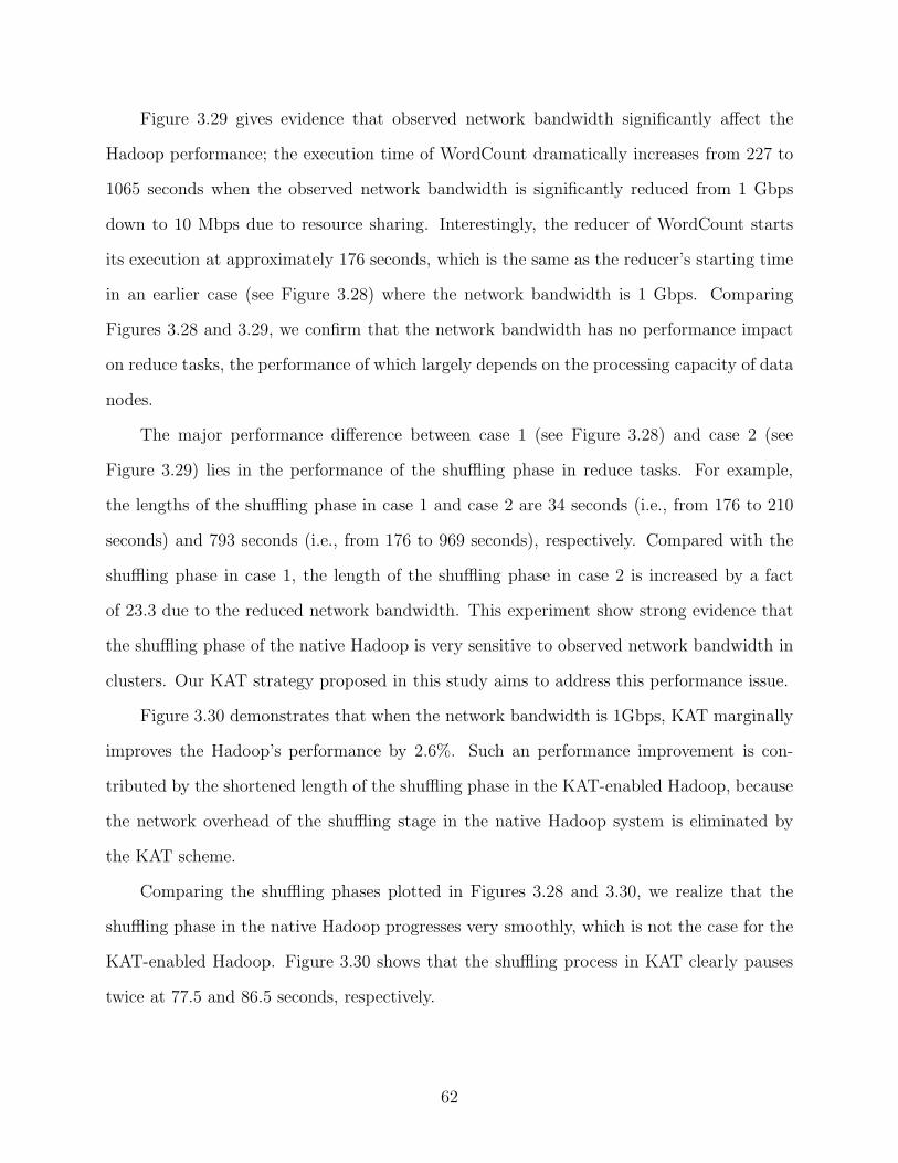
Figure 3.29 gives evidence that observed network bandwidth significantly affect the

Hadoop performance; the execution time of WordCount dramatically increases from 227 to

1065 seconds when the observed network bandwidth is significantly reduced from 1 Gbps

down to 10 Mbps due to resource sharing. Interestingly, the reducer of WordCount starts

its execution at approximately 176 seconds, which is the same as the reducer’s starting time

in an earlier case (see Figure 3.28) where the network bandwidth is 1 Gbps. Comparing

Figures 3.28 and 3.29, we confirm that the network bandwidth has no performance impact

on reduce tasks, the performance of which largely depends on the processing capacity of data

nodes.

The major performance difference between case 1 (see Figure 3.28) and case 2 (see

Figure 3.29) lies in the performance of the shuffling phase in reduce tasks. For example,

the lengths of the shuffling phase in case 1 and case 2 are 34 seconds (i.e., from 176 to 210

seconds) and 793 seconds (i.e., from 176 to 969 seconds), respectively. Compared with the

shuffling phase in case 1, the length of the shuffling phase in case 2 is increased by a fact

of 23.3 due to the reduced network bandwidth. This experiment show strong evidence that

the shuffling phase of the native Hadoop is very sensitive to observed network bandwidth in

clusters. Our KAT strategy proposed in this study aims to address this performance issue.

Figure 3.30 demonstrates that when the network bandwidth is 1Gbps, KAT marginally

improves the Hadoop’s performance by 2.6%. Such an performance improvement is con-

tributed by the shortened length of the shuffling phase in the KAT-enabled Hadoop, because

the network overhead of the shuffling stage in the native Hadoop system is eliminated by

the KAT scheme.

Comparing the shuffling phases plotted in Figures 3.28 and 3.30, we realize that the

shuffling phase in the native Hadoop progresses very smoothly, which is not the case for the

KAT-enabled Hadoop. Figure 3.30 shows that the shuffling process in KAT clearly pauses

twice at 77.5 and 86.5 seconds, respectively.

62

Figure 3.31 reveals that when the observed network bandwidth is low (e.g., 10 Mbps),

KAT speeds up the performance of the native Hadoop system by a factor of 4.35 (i.e., the

execution time of WordCount is reduced from 1065 seconds to 245 seconds). Unlike the

shuffling phases depicted in Figures 3.29 and 3.30, the shuffling phase in Figure 3.31 makes

very smooth progress during the interval between 176 and 229 seconds. This performance

trend is reasonable, because input data are better balanced in the KAT-enabled Hadoop

than in the native Hadoop.

Now let us take a close look at the map phases plotted in Figures 3.28 - 3.31. An

important observation drawn from Figure 3.28 - Figure 3.31 is that KAT allows the map tasks

to make very little progress after the reduce tasks start their execution. This performance

trend is more pronounced when the observed network bandwidth is as low as 10 Mbps. For

example, the map tasks make as little as 1% progress in the KAT-enabled Hadoop after

the reduce tasks get started (see Figure 3.31); in the native Hadoop, the map tasks make

more than 22% progress after the reduce tasks start at 176 seconds (see Figure 3.29). Map

tasks does not make any noticeable progress in the KAT-enabled Hadoop, because KAT well

balance input data sets across all the data nodes of the cluster. When it comes to KAT,

there is no demand for the map tasks to further process input data during the shuffling

phase, because the amount of data migrated among the data node is significantly reduced

by the KAT scheme.

As aforementioned experimental results confirm that KAT speeds up the performance

of the native Hadoop system when the network bandwidth is set to both 1 Gbps and 10

Mbps. The performance improvements become possible, because KAT significantly reduces

network transfer overhead induced by intermediate data. Therefore, reduce tasks in the

KAT-enabled cluster are not slowed down in order to wait for data transferred from remote

nodes to local ones.

63

3.6 Summary

In this study, we observed that a performance bottleneck in Hadoop clusters lies in the

shuffling stage, in which a large amount of intermediate data is transferred among data nodes.

The amount of transferred data heavily depends on locations and balance of intermediate

data with the same keys. To solve this performance problem, we proposed a key-aware

data placement strategy or KAT for Hadoop clusters. The pre-calculation module yields

intermediate keys for data entries prior to the shuffling stage of Hadoop applications; the

data distribution module allocates data according to pre-calculated keys made by the first

module. KAT reduces the amount of transferred intermediate data during the shuffling

phase by keeping data with the identical key to the same node. Consequently, the KAT

strategy successfully alleviates the performance-bottleneck problem introduced by excessive

data transfers.

After implementing KAT in the Hadoop distributed file system (or HDFS, for short), we

evaluated the performance of KAT on an 8-node Hadoop cluster using two real-world Hadoop

applications - Grep and WordCount. The experimental results show that KAT reduces the

execution times of Grep andWordcount by up to 21% and 6.8%, respectively. We also applied

the traffic-shaping technique to resemble real-world workloads where multiple applications

are sharing network resources in a Hadoop cluster. We evaluated the impacts of observed

network bandwidth on the performance of KAT. The empirical results indicate that when

observed network bandwidth drops down to 10Mbps, KAT can shorten the execution times


64

Chapter 4

Energy-Efficient HDFS Replica Storage System

In this Chapter, we propose a new replica architecture design that reduces the energy

consumption of redundancy-based HDFS distributed file systems. The core conception of

our approach is to conserve power consumption caused by extra data replicas. There are two

steps towards achieving high energy efficiency of the HDFS system. First, all disks within

in a data node are separated into two categories: primary replicas are stored on primary

disks and replica copies are stored on backup disks. Second, disks archiving primary replica

data remain running while backup disks are placed into the sleep mode. The backup disks

may be waked up under two conditions: (1) any primary disk fails and (2) local machines

finish processing their local primary data and start help other machines to process data.

Under these conditions, corresponding sleeping disks are waked up and provide I/O service.

Theoretically speaking, our approach can reduce at least 50% of power consumption in

a replica-based storage system. The energy efficiency of our proposed scheme can further

increase when the number of backup disks is goes up. Our method saves energy at the cost of

increasing the overhead of accessing backup disks. Although such overhead have performance

impacts on heterogeneous systems, the overhead is marginal in a balanced system. In our

architecture, multiple techniques are used to predict the usage of backup disks in order to

reduce the wakeup overhead. We implement the energy-saving scheme in the HDFS system,

which manages the power states of all disks in Hadoop clusters. In the future, we will

optimize the wakeup prediction modules to further reduce the energy-saving overhead.

65

4.1 Introduction

Evidence show that new data placement strategies could not only improve system per-

formance, but also save energy consumption in Hadoop clusters. In the first part of this

dissertation research, we develop a novel data placement strategy to boost performance of

Hadoop clusters. Now we are in a position to address an important energy-efficiency issue

in Hadoop clusters. Processors, storage, and network interconnects are three main power-

consuming components. Our preliminary results show that it is feasible to save energy in the

computing and data nodes of a Hadoop cluster. We start addressing the energy-efficiency

issue by focusing on data storage in Hadoop clusters. We aim to develop energy-efficient

data placement schemes without negatively affecting computing performance.

4.1.1 Motivation

There are three factors motivate us to investigate the energy-efficiency issue in the

Hadoop Distributed File System (HDFS). Energy-efficient HDFS can reduce operational

cost of data centers by cutting large electrical bills. The cooling cost of data centers also

will be reduced if energy-efficient HDFS is deployed. Because saving cooling cost is out the

scope of this dissertation research, let us consider the following three motivations related to

energy-efficient Hadoop clusters.

• Data replicas can be used to improve both reliability and performance in clusters.

• Using multiple disks within a data node can offer fault tolerance.

• Power can be saved by placing disks archiving replicas into the low-power mode.

Applying data replicas in HDFS can achieve high reliability and performance. To main-

tain high data availability, one can place data replicas across multiple data nodes. If one

data node fails, data replicas stored on other nodes can be used to recover such a failure.

Data stored in the failed node will be restored from the extra copies from other surviving

66

nodes. Original data might be modified by mistakes; data replicas allow users to recover

the modified data back to the previous version. In the Hadoop system, fault tolerance is

a salient feature over the other parallel computing models like MPI. The fault tolerance

becomes possible in Hadoop clusters thanks to data replicas in HDFS.

In addition to high reliability, replica data can boost I/O performance of the Hadoop

system through. Our earlier studies show that network data transfer in HDFS is very expen-

sive when network resources are shared among various applications. Keeping replica copies in

Hadoop cluster can save data transfer time while improving the overall system performance.

This is especially true when it comes to heterogeneous clusters, where some nodes finish

processing local data earlier than other nodes due to heterogeneity in computing. When fast

nodes store replicas of local data of slow nodes, the fast nodes can help the slow nodes to

process data without migrating data from the slow nodes. In other words, keeping extra

copies for local data of the slow nodes on the fast nodes reduces the amount of transferred

data from the slow to fast nodes.

Our energy-saving scheme described in this Chapter is motivated by another fact that

each data node in modern Hadoop clusters contains multiple disks. In a special case where

each node consists of a single disk, it is impossible to frequently put the disk into the low-

power state unless I/O load is extremely low. Multiple-disk-equipped data nodes boost

system availability; one disk’s failure does not lead to the failure of the entire data node.

On the other hand, it is more cost-effective to leverage multiple small disks rather than one

single large one. The capacity of a hard drive depends on the hardware techniques; disk price

exponentially increases when the increase of disk capacity. Instead of deploying a single disk

with large capacity in a data node, it is cost-effective to build a virtual large disk using

multiple inexpensive small disks. Experiment results indicate that the Hadoop performance

of using multiple disks is even higher than using a single disk array, because Hadoop can

utilize multiple CPU cores to run multiple jobs accessing different files at the same time.

Our experiments also show that there is no need to deploy an expensive high-performance

67

single disk in each node of the Hadoop system. Many Hadoop applications does not benefit

a whole lot from high I/O throughput of the expensive single disks.

In this chapter, we propose an approach to conserving energy of Hadoop clusters by

placing a large number of backup disks into the low-power mode. The contributions of our

approach are summarized as follows.

• We categorize data replicas into two camps: primary copies and backup copies. Pri-

mary copies are the core data processed by map and reduce tasks. Backup copies are

used to recover primary copies in case of any disk failure. Backup copies also will be

used to improve system performance by eliminating unnecessary data migration from

slow nodes to fast nodes.

• We design a novel data placement scheme to place primary data and backup replicas on

multiple disks of each data node. In the native HDFS of the Hadoop system, all replica

copies are treated equally and stored on disks in a mixed manner. In our new scheme,

the primary data and backup replicas are stored in a way so that primary and backup

disks can apply different power management to save energy. In particular, primary

disks are controlled by the traditional power management module; the backup disks

are manipulated by a new power management module. Backup disks are placed into

the standby mode for a long period of time when the disks are sitting idle. When a data

node or a disk fails, corresponding backup disks are waked up to continue providing

I/O service.

• We address the overhead issue of waking up backup disks by proposing two methods

to reduce I/O delays incurred by our new power management module. In the first

approach, we use RAID-5 as backup disks, because the primary goal of backup replicas

is to recover the primary replicas as quickly as possible. RAID-5 is a disk array

that offers high I/O throughput and good reliability for backup disks. The second

method is to hide the disk wakeup overhead by predicting when backup disks will

68

wakeup. Our preliminary results show that our scheme can significantly reduce the

power consumption of HDFS in Hadoop clusters.


4.2.1 RAID Based Storage Systems

Redundant array of independent disks (RAID) is a storage technique combining multiple

disks to form one unit to provide high I/O throughput and reliability [35]. RAID was first

introduced by Patterson, Gibson, and Katz in year 1988 [36] with the name of ”redundant

array of inexpensive disks”. RAID has seven levels starting from level 0 to 6. Two goals to be

achieved by all the levels of RAID are high performance or/and reliability. Prior research [10]

shows that disk arrays are a good candidate for high I/O performance and reliable secondary

storage. Among all the RAID levels, the most popular schemes are RAID-1 and RAID-5.

RAID-1 provides data mirroring without parities or striping. RAID-1 improves data

reliability by storing data identically on two disk devices. If there one disk fails, another

disk can continue I/O services. And RAID-1 can improve read performance with appropriate

operating system supports. However, RAID-1 has low space efficiency, because 50% disk

space is reserved for data mirroring.

Unlike RAID-1, RAID-5 employs data-block-level striping with distributed parities,

thereby improving both data reliability and performance without paying huge amount of

extra space. RAID-5 tolerates one disk failure; a failed disk can be rebuilt from other sur-

viving disks and parity blocks. RAID-5 is a parallel storage system providing high I/O

performance. Since parity blocks are distributed stored on all the disks in RAID-5, none of

the disks becomes a performance bottleneck of the disk system. Space efficiency of RAID-5

is high; for example, in a four- disk RAID-5, extra space for parity blocks wastes only 25%

of total disk space.

69

4.2.2 Power Savings in Clusters

A previous simulation study shows how to turn off a subset of storage nodes during

the periods of low utilization to save energy in clusters [3]. On the other hand, Willis

and Jignesh modeled a few energy-saving strategies and suggested that turning off a subset

nodes of MapReduce clusters is not an efficient way of saving energy in most cases [26]. A

handful of researchers have been working on the nature of power conservation techniques.

For example, Meisner et al. show much of power consumed by data centers is wasted in

idle systems. They propose PowerNap to quickly transition between a high-performance

active state and a low-power state [31]. Prior to that study, many schemes were proposed to

dynamically change CPU frequencies to save processor power without noticeably reducing

performance. For example, high energy efficiency can be achieved in server clusters by

lowering CPU frequency while maintaining good Quality of Service (QoS) during the non-

busy periods [41]. When we reduce the power consumption of computing clusters, the power

usage of cooling systems is reduced accordingly [5].Bash and Forman suggested to save power

of a cooling system by placing clusters in geographic locations [5]. And Facebook uses the

same strategy to place clusters in Oregon to utilize the cool and dry weather helping them

to cool down machines in the Facebook data centers.

Leverich and Kozyrakis developed an energy-efficient Hadoop cluster, where energy con-

sumption is saved by the scaling-down method [28]. GreenHDFS was proposed by Kaushik

and Bhandarkar in 2010 to save the energy from the cold zone data in HDFS [24, 25]. For

MapReduce clusters, some scheduling algorithms help in saving energy consumption. For

example, Yigitbasi proposed an energy-efficient workload scheduling to conserve energy in

heterogeneous clusters [55]. After examining the existing methods of energy saving in clus-

ters, we investigate a novel approach to conserving energy in Hadoop clusters through data

placement.

70

4.2.3 Disk Power Conservation

Magnetic disks are the most widely used storage systems in the IT industry. High

power consumption is one of a challenge issue facing large-scale data-intensive applications.

A recent study shows that energy efficiency of storage systems can be enhanced by adjusting

different disk speed and prefetching techniques [43, 8]. Narayanan proposed the write off-

loading strategy backing up the solution of spinning down disks on the aspect of writes

performance [33]. Redundancy based cache design for energy-efficient and high-performance

storage system is also available for single-speed disks [54]. Different energy conservation

techniques are employed in disk arrays [37, 29]. Lang et al. made use of data replicas to save

energy in disk arrays [27]. A similar replica scheme was proposed by Huang et.al to achieve

high energy efficiency and good I/O performance [19].

4.3 Design and Implementation Issues

Each data node in a Hadoop cluster consists of multiple disks, among which some disks

store primary copies and others store backup copies. Primary disks are likely to be kept

in the active mode, whereas backup disks are placed in the low-power mode to conserve

energy. The native HDFS is not aware of primary and backup disks in Hadoop clusters,

thereby being unable to improve energy efficiency of backup disks. In the native HDFS, all

the replicas are managed by the name node of a Hadoop cluster. The name node treats

every data replica exactly in the same way without addressing the energy-efficiency issue. In

this section, we describe how to extend the HDFS design to make this distributed file system

energy efficient. To design the energy-efficient HDFS, let us address the following issues in

the subsequent sections.

• Replica Management.

• Power Management.

• Putting Disks into the Standby Mode.

71

Figure 4.1: Architecture Design of the Energy-Efficient HDFS

• Accessing Backup Disks.

• Performance Optimization.

4.3.1 Replica Management

Replica Management is the most important and critical component in the design of the

energy-efficient HDFS. All the other components relies on the replica management module

to save energy consumed in HDFS. Recall that data managed by HDFS are divided into two

camps - primary data and backup replicas. Regardless the number of replicas for each input

file, there is only one primary copy of the data and all the other copies are considered as

backup replicas.

The goal of the energy-efficient HDFS is to save energy by putting disks storing backup

replicas into the standby mode for a long period of time. Note that a primary copy and its

72

Namenode

Datanode1 Datanode2 Datanode3

DataContent

Nodelist:1,2,3

ReplicaBit:False

DataContent

Nodelist:2,3

ReplicaBit:True

DataContent

Nodelist:3

ReplicaBit:True

Number of Replica : 3Each Data Package Includes:

1. The content of data2. List of Destination Datanodes3. Boolean ReplicaBit

Figure 4.2: Data Flow of Copying Data into HDFS

backup replicas are identical; however, the primary copies and backup replicas are located

on multiple disks of different data nodes. Figure 4.1 shows an example where each data

set has a primary copy and a backup replica. Figure 4.1 depicts the hardware architecture

for the replica management design, where each data node is comprised of two independent

disks. The master node (i.e., the name node in HDFS) is copying four individual blocks into

four data nodes. As we can see from Figure 4.1, the primary copy of each block resides on a

disk different from those storing the backup replicas. Since the backup replicas are identical

to their primary copy, each replica consumes the same disk space as its primary copy. It

is straightforward to configure disks in each data node according to the number of replicas.

For instance, in the case demonstrated in Figure 4.1 where the number of replicas is 2, each

data node contains two disks with the same capacity; one disk stores primary copies and

another disk is dedicated to backup replicas.

After describing the system architecture, we present a data flow of creating data sets to

be archived in the energy-efficient HDFS. Figure 4.2 shows the data flow diagram that reveals

how data blocks are distributed among data nodes in HDFS. The primary copies of data

blocks are delivered by the name node and stored in the first data node (i.e., Datanode1).

Then, backup replicas of the primary copies are created and transferred from the first data

73

node the second data node (i.e., Datanode2). Similarly, backup replicas are passed from the

second data note to the third one. Backup replicas are repeatedly created across multiple

data nodes until the HDFS reaches the number of replicas specified in the configuration. All

the data nodes is pre-selected by the name node and saved as a list along with the data

package. Each data node removes its name from the data-node list after receiving data blocs

from the predecessor node. For example, the list contains node 1, 2, and 3 before node

1 stores primary copies; the list contains only node 2 and 3 after node 1 finishes storing

the primary copies. After the last data node finishes creating replicas, the data-node list

becomes empty.

In addition to the data-node list transferred along with data copies, we introduce an

extra bit called replica bit to identify primary copies and backup replicas. When the replica

bit is false, a data package will be processed as a primary copy and stored on primary disks.

Otherwise, the data will be treated backup replicas and stored on backup disks. For example,

in Figure 4.2, the replica bit for node 1 is set to false, meaning that data copies stored in

node 1 are primary copies. The replica bits for node 2 and 3 are set to true, which indicates

that backup disks in node 2 and 3 are used to save backup replicas.

Creating data replicas and store them on primary and backup disks can help in reducing

disk failure rates. For example, disks with high failure rate can be utilized as backup disks,

because backup disks are rarely used compared to their primary counterparts. To improve

I/O performance, we use disks offering high I/O throughput as primary disks. Configuring

disks in this way can maximize disk utilization and data availability. Primary copies, which

are treated as popular data sets in our design, are all resides on high-performance disks to

provide fast and reliable services.

4.3.2 Power Management

Each data node in a Hadoop cluster manipulates both primary and backup disks (see

Figure 4.1); our scheme strives to turn all backup disks into the standby mode after all

74

backup replicas are generated. In our implementation, we make use of a Linux system

call to put disks in the standby mode. The design challenge is when to invoke this Linux

system call to place the backup disks into the standby mode. Disk power transitions are

governed by a power management policy. In this Section, we introduce the design of the

power management policy as well as its implementation in the Hadoop system.

Distributing Primary Copies and Backup Replicas

The first challenge is how to separate backup replicas from their primary copies and

distribute them on multiple disks. In the Hadoop configuration files, there is an item speci-

fying the directory of HDFS data storage. Separating backup replicas from primary copies

is more than simply adding a backup replica directory into the configuration file.

Let us first introduce the process of copying multiple replicas into HDFS data nodes.

As mentioned in the previous section, primary copies and their backup replicas are identical

in terms of data content. And during the data copying process, we add the replica bit along

with data packages to indicate whether a package is a primary copy or a backup one. The

replica bit changes when the data packages are passed from one data node to another node.

Only the first data node receiving data packages has the replica bit set as false. All the other

data nodes receiving the same packages have the replica bit set as true.

Upon receiving data packages, a data node first checks the replica bit. If the replica

bit is false, then the packages should be treated as primary copies to be stored in primary

disks of the data node. When the replica bit is set to true, the packages must be treated as

backup replicas to be stored on backup disks in the data node. In doing so, primary copies

and backup replicas are stored in primary and backup disks, respectively.

In addition to separating backup replicas from their primary copies, separated data

blocks have to be readily accessed by Hadoop applications. Accessing data replicas can be

easily done in the following way. One convenient approach to making HDFS access multiple

disk locations is to change the configuration file in HDFS. The configuration file, supporting

75

both the reading and writing process, has one item named ”dfs.data.dir”. The value of this

item controls locations where HDFS stores and reads data copies. In our implementation,

we extend the ”dfs.data.dir” item in a way that locations of both primary copies and backup

replicas are specified and separated using comma. In order to change the locations of backup

replicas, we add an item - ”dfs.replica.dir” - in the configuration to identify the location of

backup data folders. In our design, data replicas are grouped into primary copies and backup

replicas located on primary disks and backup disks, respectively.

Putting Disks into the Standby Mode

After primary and backup replicas are respectively stored in primary and backup disks,

the backup disks can be put into the standby mode to conserve energy. Power state transi-

tions of backup disks introduce overheads in both performance and energy consumption. For

example, transitioning back from the standby mode to the active mode inevitably increases

time spent in accessing replicas on disks. Backup disks can be placed into the standby mode

either automatically or manually. We are able to adjust the disk power management policy

by setting a standby timeout; disks are automatically placed into the standby mode after

being sitting idle for a certain time period (i.e., timeout). We make use of the hdparm

command to manage disk power states by setting multiple parameters. In the automatic

approach, we use hdparm to set the timeout period to dynamically turn disks into standby.

On the other hand, we manually execute hdparm to force target disks to switch into the

standby mode. Note that when we manually control disk power, the parameters in hdparm

are disabled; rather, the sleep parameter can put the disks into the standby mode. In sum-

mary, both method allow our disk power manager to place backup disks into the standby

mode in HDFS.

76

Accessing Backup Disks

Disks in the standby mode are waked up if any data stored on them are accessed. To

avoid the frequent power-state transitions, we strictly control the number of transitions. And

the disk power manager embedded in HDFS manipulates backup disks’ power status. Both

the automatic and manual methods are implemented in the power manager. The automatic

and manual schemes are cooperating together to manage the power states of backup disks in

HDFS. The manual scheme manages the power of backup disks when the disks are intensively

reading or writing data during the data copying process or recovering process. Copying data

into HDFS and recovering any failed disks tiger disks issue a large number of writes and

reads in a short period of time. During the copying and recovering processes, the disk power

manager performs in the manual model. In all the other cases, the disk power manager

works in the automatic mode. If a disk has been sitting idle for a period of time since

the last access, the standby mode is triggered. These cases include data content updates,

synchronization, and meta data updates.

In heterogeneous clusters, processing heterogeneity raise another performance optimiza-

tion issue. Because computing capability of data nodes in a heterogeneous cluster may dra-

matically vary, data are likely to be migrated from slow data nodes to fast data ones thanks

to the load balancing mechanism in Hadoop. Backup replicas can be used to speed up map

processes by eliminating time spent in transferring migrated data from the slow nodes to the

fast ones. Rather than migrating data from slow nodes, replicas of primary copies stored in

the slow nodes can be archived in the backup disks of the fast nodes. In doing so, migrated

data no longer need to be transferred from the slow nodes, since data replicas can be found

in the backup disks of the fast nodes.

In last paragraph, we mentioned about avoiding the access to the backup replica disks.

To address the heterogeneity issue in Hadoop, we extend the original design of energy-efficient

HDFS. We split the dfs.data.dir values into two categories - primary-copy directories and

backup-replica directories. In the earlier version of our design, backup replica directories

77

1 Runtime r = Runtime . getRuntime ( ) ;2 t ry3 {4 /∗5 ∗ Here we are execut ing the UNIX command hdparm f o r d i sk mode ope ra t i on .6 ∗ The tex t returned i s system message from execut ing the hdparm command7 ∗ This message could be s to r ed in l og f i l e f o r fu tur e i n v e s t i g a t i o n8 ∗/9 Proces s p = r . exec ( ” sudo hdparm −Y /dev/sdb” ) ;

10 BufferedReader br = new BufferedReader (new InputStreamReader (newBufferedInputStream (p . getInputStream ( ) ) ) ) ;

11 // Read the feedback and output the message from system12 St r ing l i n e ;13 whi le ( ( l i n e = br ( ) ) != nu l l )14 {15 System . out . p r i n t l n ( l i n e ) ;16 }17 // Check f o r l s f a i l u r e18 } catch ( IOException e )19 {20 System . e r r . p r i n t l n ( e . getMessage ( ) ) ;21 }

Listing 4.1: Java System Call Source Code

are implemented as a stand alone item in the configuration file. HDFS accesses data in

primary disks in most cases. If backup replicas must be accessed to avoid aforementioned

data migrations, HDFS will provide the addresses of the required data blocks to let Hadoop

access the data from the backup disks. Please note that a short time period to wakeup a

backup disk before backup replicas can be accessed.

Java System Call

In Section 4.3.2, we proposed two power management schemes. The default scheme can

be implemented by specifying the timeout parameters in the hdparm configuration file under

the etc directory in the Linux system. On the other hand, the manual power management

scheme implemented in the Java language has to be incorporated into HDFS. The integration

is accomplished by the Java system call function executing the system command inside a

java process.

78

In code listing 4.1, we present a fraction of the code as an example of executing a Linux

command inside HDFS using Java. Executing the Linux command using the Java language

offers two immediate benefits. One is that it allows us to change the disks’ power mode as

the same as what we did using Linux command. Since Java is a high level language without

low level system control interfaces, using Java system call provides a convenient channel to

achieve our goal. On the other hand, using Java system call allows HDFS to directly control

system call commands and to seamlessly cooperate with the local file system. This approach

makes it possible for other researchers to apply other power management strategies in HDFS

in the future. After such an extension, HDFS is able to collaborate with the local file system.

Our integration fills up the gap between HDFS and the local system.

4.3.3 Performance Optimization

With our energy-efficient HDFS in place, the energy efficiency of the Hadoop system is

improved by keeping backup disks in the standby mode for a long period of time. We observe

that it takes extra overhead to transit disk power from the standby mode. There are three

general approaches to tackling this performance problem. First, one can deploy disks with

short power-state transition time to immediately reduce the overhead. Second, reducing the

number of power-state transitions can substantially minimize overheads caused by power-

state transitions. For example, employing disks with low failure rates can help in reducing

the number of power transitions incurred by disk recovery. on the backup replica disks.

Third, we can develop prediction algorithms to hide the delays introduced by power-state

transitions. For example, if we can accurately predict the time at which backup disks should

be waked up, then HDFS can wake up the backup disks a few seconds prior to that time.

Thus, when the backup disks are about to be accessed, they have already been transited

back to the active mode.

79

Deploying RAID in HDFS

We decide to deploy RAID in HDFS to offer high I/O throughput and low data failure

rate. Please refer to Section 4.2.1 for the background of the RAID systems and all different

RAID levels. In our design, we choose to use RAID-5 as backup disks to optimize the perfor-

mance of energy-efficient HDFS. Recall that RAID-5 has a block level striping structure (see

Section 4.2.1), meaning that data can be accessed in parallel to achieve high I/O throughput.

RAID-5 can continuously provide I/O service even in case of one failed disk in the array.

The failure rate, R, of RAID-5 is expressed as Equation 4.1 in terms of the number of drives,

n, and the drive failure rate, r. In this reliability model, disk drives in the array are identical

and independent of each others.

R = n(n− 1)r2 (4.1)

Another advantage of RAID-5 is that parity blocks are uniformly distributed across

on all disks; as a result, no disk becomes performance bottleneck in RAID-5. Although

RAID-5 improves the overall performance by the virtue of high I/O throughput, employing

RAID-5 does not affect or hide performance delay caused by disk power-state transitions.

In the native Hadoop system, high disk I/O throughput might not be needed, because in

many Hadoop applications, the memory and CPUs of Hadoop clusters rather than disks are

performance bottlenecks. Unlike traditional Hadoop, our energy efficient HDFS relies on

RAID-5 to offer high-performance I/Os for back replicas. In homogeneous clusters, backup

replicas are rarely accessed as local mappers’ inputs; in most cases, the backup replicas are

used to recover failed disks where primary copies must be recovered. During the primary

disk recovery process, RAID-5 can quickly access backup replicas in parallel. Thus, RAID-5

substantially speeds up the data recovery process.

80

Prediction for Wake-Ups

RAID-5 improves the overall performance of energy efficient HDFS. However, RAID-

5 can not eliminate delays caused by power-state transitions. This fact motivate us to

investigate prediction solutions that can help to hide the performance delays in energy-

efficient HDFS.

The prediction module aims to waking up backup disks a few seconds prior to the time

when the backup disks must be active. Waking up the disks in advance can guarantee that

the backup disks are in the active mode when the disks are about to be accessed.

Pay attention to access patterns of backup replicas, we observe that backup replicas are

only accessed in a few cases described in Section 4.3.2). Some cases can be directly predicted

whereas others can not be predicted without hints provided by applications. Note that it

is extremely difficult if not impossible to predict the time when primary disks encounter

failures.

Now let us consider a case where accesses to backup replicas can be predicted. Data

nodes are aware of data being processed and data left over to be processed. Data nodes keep

track of primary-data processing, being aware of when the process will be finished. When

map tasks fetch the last block of primary data, backup disks are immediately waked up by

HDFS. After waking up the backup disks in advance, the following steps will be performed.

First, if the primary copies of those backup replicas has not been finished yet on the other

slow data nodes, the map tasks on the local fast nodes continuously process the unprocessed

data content loading from the backup disks. Second, when the Hadoop system is about to

finish, backup disks are ready to store the backup replicas of the processes’ results.

The prediction module aims to hide the latency incurred by power-state transitions in

backup disks. The overall performance of energy-efficient HDFS is improved by applying

the prediction module to wake up backup disks in advance. Different prediction algorithms

lead to various performances and energy efficiencies. The goal of the prediction algorithms

81

is to make good tradeoffs between performance and energy savings. Such tradeoffs can be

managed by system administrators of Hadoop clusters.

4.4 Experimental Results

In this section, we conduct preliminary tests to compare the energy efficiency and per-

formance of our energy-efficient HDFS system against the native HDFS. We start this section

by introducing the experiment settings. After presenting performance analysis, we provide

suggestions on how to configure energy-efficient HDFS based on workload conditions.

4.4.1 Experiments Setup

Table 4.1: Energy-Efficient HDFS Cluster SpecificationsType Hardware Software

1×Intel Xeon 2.4 GHz processor Ubuntu 10.04Name 1×4 GBytes of RAM Linux kernel

2.6.23Node 1×1 GigaBit Ethernet network card Hadoop 0.20.2×1 1×Seagate 160 GB SATA disk

Intel Xeon 2.4 GHz processor Ubuntu 10.04Data 2 GBytes of RAM Linux kernel

2.6.23Node 1 GigaBit Ethernet network card Hadoop 0.20.2×3 1×Seagate 500 GB SATA disk

1×1.5 TB external SATA Disk Array of RAID 5

We carry out a set of experiments on a 4-data-node cluster. Table 4.1 shows the hardware

specifications of the tested cluster containing two types of nodes - namenode and data nodes.

The namenode controls all the data nodes of the cluster and schedules tasks during the course

of applications’ executions. The three data nodes store all primary and backup replicas. The

namenode in our energy-efficient HDFS is similar to that of the native HDFS in terms of

hardware configuration, because the namenode is energy-efficient at the software level. The

data nodes in the energy-efficient HDFS is different from the native HDFS with respect to

both hardware and software. For example, each data node in the energy-efficient HDFS

82

consists of an external RAID-5 disk array serving as backup disks. In addition, each data

node is comprised of an energy-efficient management module.

In many cases, primary and back disks in a data node are identical. Nevertheless,

it is not assumed, by any means, that disks in data nodes are homogeneous. Data disks

and backup ones may be heterogeneous in terms of both capacity and performance. In our

testbed, we an input data set of 75GB consists of 150 text files (500MB/file), which are

evenly distributed on three data nodes with 25 GB primary data residing on each primary

replica disk. These data files only require 150GB space to accommodate two backup replicas

on the three data nodes when the number of replicas is set to 3. The capacity of external

disk arrays in the testbed meets the space requirement. We use a power meter (i.e. P4400

Kill A Watt) to measure the energy consumption of the tested cluster. The measurement

errors of P4400 is below 0.2%. Each data node and its disk array are connected to a power

meter used to measure power usage.

4.4.2 What Do We Measure

The primary goal of energy-efficient HDFS is to reduce energy consumption caused

by data nodes in a Hadoop cluster. Normally, high energy efficiency comes at the cost

of performance. In our experiment, we also measure response times to quantify impact

energy-efficient HDFS on the performance of the tested cluster. The power consumption is

measured in the unit of KWH, whereas response time is recorded in minute. The minimum

unit measured by the P4400 power meters is 0.01 KWH, which is considered as a large value

for each data-node’s power measurement. To address this issue, we increase the size of input

data sets to boost the data nodes’ power consumption that can be accurately measure by

P4400. The power consumption of each data node ranges anywhere from 70 to 120 watts.

We run WordCount as a benchmark application on the tested Hadoop cluster, because

WordCount is a real-world read-intensive Hadoop application. Note that WordCount is a

very popular benchmark used to evaluate performance of Hadoop clusters.

83

!"#$ %%!"#$ &'(

)*+ ,-./+0*.12 ,-+*.1/+0* ,3*

,4

1,4

.,4

5,4

/,4

*,,4

*1,4

*.,4

*5,4

*/,4

67%89:;6<=>%7?4!"#$4 @8>9>7&A4!"#$4

!"#$%&#"'()*

"'+*)&,-".'

Figure 4.3: Wordcount execution times of the energy efficient HDFS and the native HDFS.

4.4.3 Results Analysis

Figure 4.3 and Figure 4.4 show both the response time and power consumption of the

energy-efficient HDFS and the native HDFS. The Figure 4.3 indicates the average running

time (measured in minutes) of the WordCount benchmark on the energy-efficient HDFS and

the native HDFS system. Figure 4.4 reveals the two HDFS systems’ power consumptions

measured in the unit of KWh. The results show that the energy-efficient HDFS consumes

0.26 KWH power during the period of 162 minutes to run the WordCount application;

the native HDFS consumes 0.32 KWH power within 153 minutes to complete the same

WordCount benchmark. The results suggest that the energy-efficient HDFS reduce the

power consumption of the native HDFS by 18.75% with a marginal increase in execution

time. The execution time of WordCount is merely increased by 5.88% in the energy-efficient

HDFS. In many applications, it is reasonable to trade 5.88% increase in execution time for

18.75% savings in energy consumption.

To quantify tradeoff between energy efficiency and performance, we introduce a indicator

PowerTime or Pt, which is a product of power cost P and response time T (see Equation 4.2).

84

!"# $%#!&#''"( $%)*")((&! $%&+$%'

!"# $%#)#"'!"# $%)#)&(*&# $%,+$%"

!"# $%##"(')") $%))&'(#&* "+$

$-

$%$#-

$%"-

$%"#-

$%'-

$%'#-

$%!-

$%!#-

./01234.5670/8-9:;<- =1727/>?-9:;<-

!"#$%&'"()*+,-"(&./012&

Figure 4.4: Wordcount power consumptions of energy efficient HDFS and the native HDFS.

The goal of the energy-efficient HDFS is to lower the Pt value, because a low value of Pt

means high energy efficiency and performance. Applying Equation 4.2 to the tested Hadoop

cluster, we obtain the Pt values of the energy-efficient HDFS and the native HDFS. Thus,

the Pt value of our HDFS is as low as 42.12 and the Pt value of the native HDFS is 48.96,

meaning that the Pt value of our system is 13.97% lower than that of the native HDFS.

Pt = P × T (4.2)

Ptc =

P/P ′ if only Power is considered

α× P

P ′+ β × T

T ′α and β are between 0 and 1, and their sum equals 1

T/T ′ if only Performance is considered

(4.3)

For some applications (e.g., real-time applications), high performance is more important

than high energy efficiency. In other applications, reducing energy consumption is more

85

!"#$

!"#%$

!"##$

!"#&$

!"#'$

!"($

!"(%$

!"(#$

!"(&$

!"#$

%&'()$)*+$,-")$.)&/-0$

)*+,+-./$0123$

4-5*,6$478+5-9$0123$

Figure 4.5: Power consumptions of Wordcount on energy-efficient HDFS and the nativeHDFS.

critical than improving performance. Ideally, we should be able to configure the energy-

efficient HDFS according to target applications’ performance requirements. We introduce

another comparison model (see Equation 4.3) to show under which circumstances our energy-

efficient HDFS outperforms the native one. The parameter P ′ in Equation 4.3 indicates the

sum of average power consumptions of the two HDFS system, whereas T ′ is the sum of

average response times of the two systems. α and β are two coefficients representing the

importance of energy efficiency and performance. Note that sum of α and β equals to 1.

Figure 4.5 shows the comparisons between the two HDFS systems under various α and β

values. The figure shows our energy-efficient HDFS achieves lower Ptc than the native HDFS

when the value of α is larger than 0.2. This result indicates that applications favouring high

energy-efficiency can obtain benefits from our energy-efficient HDFS.

86

4.4.4 Discussions and Suggestions

We observe from Figure 4.4 that the energy-efficient HDFS improve the energy efficiency

of the native HDFS. Although our implementation is independent of any specific Hadoop

applications, the performance and energy efficiency of our system largely depends on I/O

access patterns of Hadoop applications. The application used to test our system is Word-

Count - a benchmark in the Hadoop example package. The WordCount application issues a

huge number of reads and very few writes to HDFS. Such an access pattern of WordCount

reduces the chance of accessing replicas located in backup disks, which explore excessive

opportunities to transit into the low-power state to conserve energy. The energy savings

provided by the energy-efficient HDFS become possible thanks to standby backup disks.

We suggest to optimize energy efficiency of Hadoop clusters by addressing the following

hardware-configuration issues. First, a disk-capacity ratio between backup disks and primary

disks relies on the number of replicas in the configuration file. For example, if the number of

replicas is n, the capacity ratio is (n-1)/1, meaning that the capacity of backup disks must

be at least n−1 times larger than that of primary disks on each data node. Second, one may

run profiling tests for target Hadoop applications on a cluster. After a few profiling tests are

completed, we can simply evaluate performance and energy efficiency of the Hadoop cluster

using appropriate α and β values depending on the requirements of the target applications.

Third, write-intensive applications receive little benefits from the energy-efficient HDFS and;

therefore, we prevent backup disks from transitioning into the standby mode under any write-

intensive workload condition. This approach allows our system keep write performance as

high as that of the native HDFS for all write-intensive applications.

4.5 Summary

In this chapter, we proposed an energy-efficient HDFS system that can conserve the

energy consumption of Hadoop clusters. Our system provides energy savings by aggressively

placing backup disks in each data note into the standby mode while keeping primary disks

87

active to ensure high I/O performance. The backup disks may be waked up if any primary

disk fails or local machines start helping other machines to process data.

We implemented and tested our idea on a small-scale cluster. The preliminary results

show that our approach improves the energy efficiency of Hadoop clusters by 13% with

marginal increases in time of accessing backup disks. Although such overhead have perfor-

mance impacts on heterogeneous systems, the overhead is marginal in a balanced system.

We suggest three ways of optimizing the energy-efficient HDFS. These methods include

(1) the configuration of the disk-capacity ratio between backup disks and primary disks;

(2) conducting profiling tests for target Hadoop applications; and (3) keeping backup disks

active for write-intensive applications. We believe that with appropriate settings, the energy-

efficient HDFS can achieve both good performance and energy efficiency for a wide range of

Hadoop applications.

88

Chapter 5

Conclusion

In this dissertation, we first proposed two data-placement strategies to improve the

performance of Hadoop cluster. Next, we described an energy-efficient Hadoop distributed

file system (HDFS). This chapter summarizes all the contributions made in this dissertation

study. Chapter 6 discusses the future work as an extension of this dissertation.

5.1 Observation and Profiling of Hadoop Clusters

We tested a Hadoop cluster using various experimental settings in order to identify

performance issues in the Hadoop system. After analyzing performance results collected

from a large set of experiments, we successfully found a few flaws and bottlenecks in the

traditional Hadoop system. We tested an array of solutions, among which only few work

well.

To better tune the performance of Hadoop clusters, we studied the impacts of system

parameters on the performance of Hadoop. Our experiments show that the block size, file

size, JVM usage, and number of map and reduce tasks are the major factors affecting the

Hadoop performance. We observed from our initial experiments that that all the above

affecting factors are somehow related to I/O usage, which in turn has significant impact on

the overall Hadoop performance.

Our earlier experiments results indicate that there exist many random I/O accesses

rather than sequence ones. Thus, we deployed solid state disks (SSDs) into the Hadoop

cluster to improve the performance of random reads and writes. The results confirm that

SSD improves the cluster performance by reducing response times of random I/O requests.

However, SSDs have some drawbacks on the write performance and the lifetime issue related

89

to writes. Since intermediate data are frequently written and read in HDFS, the lifetime

of SSDs are likely to be shorten by write-intensive applications. To solve this problem,

we proposed a hybrid solution combining SSDs with hard drives in HDFS of the Hadoop

cluster. SSDs store original input files, which are read multiple times once they are available

in HDFS. Then, we configured HDFS in a way to allow hard drives handle intermediate

data, which have no impact on the lifetime of the hard drives.

In this part of work, we identified that small file accesses downgrade system performance.

Small blocks in HDFS cause frequent job exchanges, which in term make CPU and disks

underutilized. A few existing scheme might offer solutions to this problem. For example, the

HAR archive is a solution that is included as part of the HDFS package. HAR groups all

small files and uses an index file to record the small file positions in a single HAR file. This

is the most convenient method to address the small-file problem, because the small files in

the HAR file can still be accessed through the index file. Once the HAR file is generated, it

can not be modified. The only way to change the file’s content is generate an new HAR file

again. Another solution is using the sequence file access function in the Hadoop APIs. The

function defined input format for map tasks, small files are considered as a single file with

different IDs. However, this approach requires an extra effort from programmers to correctly

format input files.

5.2 KAT Data Placement Strategy for Performance Improvement

we observed that a performance bottleneck in Hadoop clusters lies in the shuffling stage,

in which a large amount of intermediate data is transferred among data nodes. The amount

of transferred data heavily depends on locations and balance of intermediate data with the

same keys. To solve this performance problem, we proposed a key-aware data placement

strategy or KAT for Hadoop clusters. The pre-calculation module yields intermediate keys

for data entries prior to the shuffling stage of Hadoop applications; the data distribution

module allocates data according to pre-calculated keys made by the first module. KAT

90

reduces the amount of transferred intermediate data during the shuffling phase by keeping

data with the identical key to the same node. Consequently, the KAT strategy successfully

alleviates the performance-bottleneck problem introduced by excessive data transfers.

After implementing KAT in the Hadoop distributed file system (or HDFS, for short), we

evaluated the performance of KAT on an 8-node Hadoop cluster using two real-world Hadoop

applications - Grep and WordCount. The experimental results show that KAT reduces the

execution times of Grep andWordcount by up to 21% and 6.8%, respectively. We also applied

the traffic-shaping technique to resemble real-world workloads where multiple applications

are sharing network resources in a Hadoop cluster. We evaluated the impacts of observed

network bandwidth on the performance of KAT. The empirical results indicate that when

observed network bandwidth drops down to 10Mbps, KAT can shorten the execution times


5.3 Replica Based Energy Efficient HDFS Storage System

To improve energy efficiency of Hadoop clusters, we proposed an energy-efficient HDFS

system that conserves energy consumption in clusters supporting Hadoop applications. The

design of our new energy-efficient HDFS provides energy savings by aggressively placing

backup disks in data notes into the standby mode while keeping primary disks active to offer

high I/O performance. The backup disks are waked up in case of any primary-disk failure

or balancing load (i.e., local machines start helping other machines to process data).

We implemented and tested our idea on a real-world Hadoop cluster. The preliminary

results show that our HDFS system improves the energy efficiency of Hadoop clusters by 13%

with marginal increases in time of accessing backup disks. We proposed three approaches to

optimizing the performance of our energy-efficient HDFS. First, we can configure the disk-

capacity ratio between backup disks and primary disks. Second, one may conduct profiling

tests for target Hadoop applications. Third, we are able to improve performance by keeping

91

backup disks active for write-intensive applications. With appropriate settings, the energy-

efficient HDFS can achieve both good performance and energy efficiency for a wide range of

Hadoop applications.

5.4 Summary

In this dissertation study, we developed two strategies to improve the performance of

Hadoop cluster by optimizing the shuffling stage where a large amount of data is transferred

among data nodes. In our approaches, data sharing the same key are not scattered across

a cluster, thereby alleviating the network performance bottleneck problem imposed by data

transfers. We also implement a prototype of the energy-efficient HDFS, which conserves

power consumption caused by extra data replicas in Hadoop clusters. We firmly believe

that the performance of our proposed approach can be further improved if solid state disks

are appropriately incorporated in Hadoop clusters to handle primary data and intermediate

data.

92

Chapter 6

Future Works

In this dissertation study, we improve both the performance and energy efficiency of

Hadoop clusters. During the course of the study, we face a variety of issues to be addressed

in our future studies. In this chapter, we briefly discuss these open issues that have not been

solved in this dissertation.

6.1 Data Placement with Application Disclosed Hints

The performance of our proposed KAT data-placement strategy largely depends on the

nature of applications. Such an application dependency is a big disadvantage of KAT, be-

cause the data-distribution module is implemented and integrated into HDFS. Nevertheless,

this issue can be addressed by using application disclosed hints. Access patterns of Hadoop

applications can be analyzed using a profiling tool, which allows application developers or

system administrators to estimate the best data-placement solutions. These pre-calculated

data-placement decisions are used as hints provided by the applications. An interface can be

implemented in HDFS to process file requests as well as performance-improvement informa-

tion issued by applications. HDFS can coordinate with the Hadoop applications to improve

the performance.

6.2 Trace Based Prediction

In Chapter 4, we introduced the prediction module for reducing the overhead caused

by disk wake-ups. In addition to this prediction method, we will develop another prediction

method that aims at using historical data to estimate the time at which any data-node

failure occurs. The disk and data node failures are not only related to application types but

93

also read and write access patterns. Recently studies show that different types of disks have

various annual failure rates. Given a Hadoop cluster, the failure rates of each data node and

its disks can be estimated from historical data (e.g., I/O traces and log files). According to

the historical access patterns recorded in the trace and log files, one may implement a module

to automatically predict data-node failures for Hadoop clusters. Based on the predictions,

corresponding backup disks will be waked up to handle potential replicas for data nodes that

are likely to fail. This proposed solution is expected to solve the disk and data-node failure

prediction problem described in Chapter 4.

94

Bibliography

[1] Azza Abouzeid, Kamil Bajda-Pawlikowski, Daniel Abadi, Avi Silberschatz, and Alexan-der Rasin. Hadoopdb: an architectural hybrid of mapreduce and dbms technologies foranalytical workloads. Proc. VLDB Endow., 2(1):922–933, August 2009.

[2] Amazon. Amazon elastic compute cloud. http://aws.amazon.com/ec2.

[3] Hrishikesh Amur, James Cipar, Varun Gupta, Gregory R. Ganger, Michael A. Kozuch,and Karsten Schwan. Robust and flexible power-proportional storage. In Proceedingsof the 1st ACM symposium on Cloud computing, SoCC ’10, pages 217–228, New York,NY, USA, 2010. ACM.

[4] apache.org. http://lucene.apache.org/hadoop.

[5] Cullen Bash and George Forman. Cool job allocation: measuring the power savingsof placing jobs at cooling-efficient locations in the data center. In 2007 USENIX An-nual Technical Conference on Proceedings of the USENIX Annual Technical Conference,ATC’07, pages 29:1–29:6, Berkeley, CA, USA, 2007. USENIX Association.

[6] B.He, W.Fang, Q.Luo, N.Govindaraju, and T.Wang. Mars: a MapReduce frameworkon graphics processors. ACM, 2008.

[7] Dhruba Borthakur. The Hadoop Distributed File System: Architecture and Design. TheApache Software Foundation, 2007.

[8] Enrique V. Carrera, Eduardo Pinheiro, and Ricardo Bianchini. Conserving disk energyin network servers. In In 17 th International Conference on Supercomputing, 2003.

[9] Barbara Chapman, Gabriele Jost, and Ruud van der Pas. Using OpenMP: PortableShared Memory Parallel Programming (Scientific and Engineering Computation). TheMIT Press, 2007.

[10] Peter M. Chen, Edward K. Lee, Garth A. Gibson, Randy H. Katz, and David A. Pat-terson. Raid: High-performance, reliable secondary storage. ACM Computing Surveys,26:145–185, 1994.

[11] C.Olston, B.Reed, U.Srivastava, R.Kumar, and A.Tomkins. Pig latin: a not-so-foreignlanguage for data processing. In SIGMOD ’08: Proceedings of the 2008 ACM SIGMODinternational conference on Management of data, pages 1099–1110. ACM, 2008.

95

[12] Tyson Condie, Neil Conway, Peter Alvaro, Joseph M. Hellerstein, Khaled Elmeleegy,and Russell Sears. Mapreduce online. In Proceedings of the 7th USENIX conference onNetworked systems design and implementation, NSDI’10, pages 21–21, Berkeley, CA,USA, 2010. USENIX Association.

[13] D.Borthakur. The Hadoop Distributed File System: Architecture and Design. TheApache Software Foundation, 2007.

[14] Jeffrey Dean, Sanjay Ghemawat, and Google” Inc. Mapreduce: simplified data process-ing on large clusters. IN OSDI’04: Proceedings of the 6th conference on symposium onoperating systems design &implementation, 2004.

[15] Jens Dittrich, Jorge-Arnulfo Quiane-Ruiz, Alekh Jindal, Yagiz Kargin, Vinay Setty, andJorg Schad. Hadoop++: making a yellow elephant run like a cheetah (without it evennoticing). Proc. VLDB Endow., 3(1-2):515–529, September 2010.

[16] Mohamed Y. Eltabakh, Yuanyuan Tian, Fatma Ozcan, Rainer Gemulla, Aljoscha Kret-tek, and John McPherson. Cohadoop: flexible data placement and its exploitation inhadoop. Proc. VLDB Endow., 4:575–585, June 2011.

[17] Archana Sulochana Ganapathi. Predicting and Optimizing System Utilization and Per-formance via Statistical Machine Learning. PhD thesis, EECS Department, Universityof California, Berkeley, Dec 2009.

[18] Hive. http://hive.apache.org/.

[19] Hai Huang, Wanda Hung, and Kang G. Shin. Fs2: dynamic data replication in free diskspace for improving disk performance and energy consumption. SIGOPS Oper. Syst.Rev., 39(5):263–276, October 2005.

[20] Infiniband. http://en.wikipedia.org/wiki/InfiniBand.

[21] Jaql. http://code.google.com/p/jaql.

[22] Dawei Jiang, Beng Chin Ooi, Lei Shi, and Sai Wu. The performance of mapreduce: anin-depth study. Proc. VLDB Endow., 3(1-2):472–483, September 2010.

[23] Henk Jonkers. Queueing models of parallel applications: The glamis methodology. InGnter Haring and Gabriele Kotsis, editors, Computer Performance Evaluation, volume794 of Lecture Notes in Computer Science, pages 123–138. Springer, 1994.

[24] Rini T. Kaushik and Milind Bhandarkar. Greenhdfs: towards an energy-conserving,storage-efficient, hybrid hadoop compute cluster. In Proceedings of the 2010 interna-tional conference on Power aware computing and systems, HotPower’10, pages 1–9,Berkeley, CA, USA, 2010. USENIX Association.

[25] Rini T. Kaushik, Milind Bhandarkar, and Klara Nahrstedt. Evaluation and analysisof greenhdfs: A self-adaptive, energy-conserving variant of the hadoop distributed filesystem. In Proceedings of the 2010 IEEE Second International Conference on Cloud

96

Computing Technology and Science, CLOUDCOM ’10, pages 274–287, Washington,DC, USA, 2010. IEEE Computer Society.

[26] Willis Lang and Jignesh M. Patel. Energy management for mapreduce clusters. Proc.VLDB Endow., 3(1-2):129–139, September 2010.

[27] Willis Lang, Jignesh M. Patel, and Jeffrey F. Naughton. On energy management, loadbalancing and replication. SIGMOD Rec., 38(4):35–42, June 2010.

[28] Jacob Leverich and Christos Kozyrakis. On the energy (in)efficiency of hadoop clusters.SIGOPS Oper. Syst. Rev., 44(1):61–65, March 2010.

[29] Dong Li and Jun Wang. Eeraid: energy efficient redundant and inexpensive disk array.In Proceedings of the 11th workshop on ACM SIGOPS European workshop, EW 11, NewYork, NY, USA, 2004. ACM.

[30] De-Ron Liang and Satish K. Tripathi. On performance prediction of parallel compu-tations with precedent constraints. IEEE Trans. Parallel Distrib. Syst., 11(5):491–508,May 2000.

[31] David Meisner, Brian T. Gold, and Thomas F. Wenisch. Powernap: eliminating serveridle power. SIGPLAN Not., 44(3):205–216, March 2009.

[32] Daniel A. Menasce, Lawrence W. Dowdy, and Virgilio A. F. Almeida. Performance byDesign: Computer Capacity Planning By Example. Prentice Hall PTR, Upper SaddleRiver, NJ, USA, 2004.

[33] Dushyanth Narayanan, Austin Donnelly, and Antony Rowstron. Write off-loading:Practical power management for enterprise storage. Trans. Storage, 4(3):10:1–10:23,November 2008.

[34] Michael Noll. http://www.michael-noll.com/.

[35] D A Patterson, P Chen, G Gibson, and R H Katz. Introduction to redundant arrays ofinexpensive disks (raid), 1989.

[36] David A. Patterson, Garth Gibson, and Randy H. Katz. A case for redundant arraysof inexpensive disks (raid). In Proceedings of the 1988 ACM SIGMOD internationalconference on Management of data, SIGMOD ’88, pages 109–116, New York, NY, USA,1988. ACM.

[37] Eduardo Pinheiro and Ricardo Bianchini. Energy conservation techniques for disk array-based servers. In Proceedings of the 18th annual international conference on Supercom-puting, ICS ’04, pages 68–78, New York, NY, USA, 2004. ACM.

[38] C. Ranger, R. Raghuraman, A. Penmetsa, G. Bradski, and C. Kozyrakis. Evaluatingmapreduce for multi-core and multiprocessor systems. High-Performance ComputerArchitecture, International Symposium on, 0:13–24, 2007.

97

[39] Mendel Rosenblum and John K. Ousterhout. The design and implementation of alog-structured file system. ACM Trans. Comput. Syst., 10(1):26–52, February 1992.

[40] R.Pike, S.Dorward, R.Griesemer, and S.Quinlan. Interpreting the data: Parallel analysiswith Sawzall, volume 13. IOS Press, 2005.

[41] Cosmin Rusu, Re Ferreira, Claudio Scordino, Aaron Watson, Rami Melhem, and DanielMoss. Energy-efficient real-time heterogeneous server clusters. In In Proceedings ofRTAS, pages 418–428. IEEE Computer Society, 2006.

[42] Ratnesh K. Sharma, Cullen E. Bash, Chandrakant D. Patel, Richard J. Friedrich, andJeffrey S. Chase. Balance of power: Dynamic thermal management for internet datacenters. IEEE Internet Computing, 9(1):42–49, January 2005.

[43] Seung Woo Son and Mahmut Kandemir. Energy-aware data prefetching for multi-speeddisks. In Proceedings of the 3rd conference on Computing frontiers, CF ’06, pages 105–114, New York, NY, USA, 2006. ACM.

[44] SSD. http://en.wikipedia.org/wiki/SSD.

[45] SSD. http://kb-zh.sandisk.com/.

[46] Chao Tian, Haojie Zhou, Yongqiang He, and Li Zha. A dynamic mapreduce schedulerfor heterogeneous workloads. Grid and Cloud Computing, International Conference on,0:218–224, 2009.

[47] Apache Tutorial. http://hadoop.apache.org/.

[48] Elizabeth Varki. Mean value technique for closed fork-join networks. In PROCEED-INGS OF ACM SIGMETRICS CONFERENCE ON MEASUREMENT AND MODEL-ING OF COMPUTER SYSTEMS, pages 103–112, 1999.

[49] Guanying Wang, Ali R. Butt, Prashant Pandey, and Karan Gupta. Using realisticsimulation for performance analysis of mapreduce setups. In Proceedings of the 1stACM workshop on Large-Scale system and application performance, LSAP ’09, pages19–26, New York, NY, USA, 2009. ACM.

[50] Apache Hadoop Wiki. http://wiki.apache.org/hadoop.

[51] W.Tantisiriroj, S.Patil, and G.Gibson. Data-intensive file systems for internet services:A rose by any other name ... Carnegie Mellon University Parallel Data Lab TechnicalReport CMU-PDL-08-114, October 2008.

[52] Jiong Xie and Xiao Qin. The 19th heterogeneity in computing workshop (hcw 2010).In Parallel Distributed Processing, Workshops and Phd Forum (IPDPSW), 2010 IEEEInternational Symposium on, pages 1 –5, april 2010.

[53] Yahoo. Yahoo! launches worlds largest hadoop production application.http://tinyurl.com/2hgzv7.

98

[54] Xiaoyu Yao and Jun Wang. Rimac: a novel redundancy-based hierarchical cache ar-chitecture for energy efficient, high performance storage systems. SIGOPS Oper. Syst.Rev., 40(4):249–262, April 2006.

[55] Nezih Yigitbasi, Kushal Datta, Nilesh Jain, and Theodore Willke. Energy efficientscheduling of mapreduce workloads on heterogeneous clusters. In Green ComputingMiddleware on Proceedings of the 2nd International Workshop, GCM ’11, pages 1:1–1:6, New York, NY, USA, 2011. ACM.

[56] Matei Zaharia, Andy Konwinski, Anthony D. Joseph, Randy Katz, and Ion Stoica.Improving mapreduce performance in heterogeneous environments. In Proceedings ofthe 8th USENIX conference on Operating systems design and implementation, OSDI’08,pages 29–42, Berkeley, CA, USA, 2008. USENIX Association.

99

improve i/o performance and energy eﬃciency in hadoop …

Documents