implications of frequency-domain inversion of earthquake ground

Geophysical Journal (1988) 94, 443-455

Implications of frequency-domain inversion of earthquake ground motions for resolving the space-time dependence of slip on an extended fault

Allen H. Olson" and John G. Anderson Institute of Geophysics and Planetary Physics, Scripps Institution of Oceanography, University of California, San Diego A-025, La Jolla, California 92093, USA

Accepted 1988 February 22. Received 1988 February 22; in original form 1987 June 23.

SUMMARY A frequency-domain method is presented in which the Fourier spectral amplitudes of observed earthquake ground motions are used as data to constrain the space-time dependence of slip on the fault. Performing the temporal deconvolution in the frequency domain allows the spatial dependence of slip at each frequency to be computed independently. This greatly reduces the computational effort and allows the grid spacing to be chosen sufficiently fine enough to form an accurate numerical approximation to the continuous problem, thereby eliminating spatial and temporal discretization effects. Time-domain methods require the specification of rupture time as a function of position on the fault in order to reduce the number of parameters in inversion. Some non-linear inversion methods iterate on the rupture time in order to find a set of rupture times which provides the best fit to the data. This non-linear restriction, and the potential bias it may introduce, is eliminated in the frequency-domain formulation.

The method is applied to synthetic test data calculated using Haskell's model of a uniform rupture in a homogeneous full-space. Three different recording geometries with characteris- tics comparable to current strong motion arrays are considered. Inversion for the slip function is demonstrated to be non-unique and a particular solution is found which minimizes the square of the slip velocity averaged over the fault surface. The minimum norm solutions have systematically lower peak slip velocities and spectra which fall off much faster than the input model ( f P 3 vs. f - ' ) . This discrepancy is shown to result from a trade-off between the spectral amplitude of slip at a point on the fault and the local phase velocity of slip propagation. The trade-off is quite large for the arrays considered, a factor of 10 to 100 at frequencies between 1.0 Hz and 2.5 Hz.

Key words: frequency-domain inversion, earthquake ground motions, rupture parameters

INTRODUCTION

Previous studies of earthquake ground motion data have utilized either matrix inversion techniques or trial and error forward modelling to construct models of the space-time dependence of slip on the fault. The strong motion data for the 1979 Imperial Valley earthquake have been the subject of several such studies. Although the data for this earthquake are extraordinarily good by current standards, both in terms of the number of stations and knowledge of crustal structure, the interpretations of the data contain substantial differences. Models presented by Hartzell & Helmberger (1982) and Hartzell & Heaton (1983) required the local rupture velocity to be less than the shear-wave speed. The 1982 study contained two localized areas of larger than average dislocation on the fault, while the 1983 study showed the two zones collapsed into a single zone.

* Present Address: Telectronics, Inc., 3368 Governor Drive Ste. F252, San Diego, CA 92122, USA.

Studies by Olson & Apse1 (1982) and Archuleta (1984), on the other hand, showed a local rupture velocity which sometimes exceeded the shear-wave speed; in Archuleta's model, it even exceeds the P-wave speed along one section of the fault. Unless one is persuaded that the goodness-of-fit in one of the studies is much better than the rest, one is left with the dilemma of how to interpret the differences. There is also the possibility that as yet undiscovered solutions might fit equally well, while having main features that are very different from the existing models.

What is found lacking in these studies is a quantitative statement as to the resolvability of features in the model. One aspect of time-domain inversion methods that makes the resolution question particularly difficult to address is the non-linear parameterization of the rupture-time variable. The rupture time at each location on the fault is fixed before inversion in order to reduce the number of parameters (slip amplitudes) which must be solved for. Different rupture- time models can be tried in an effort to find a good one;

443

Dow

nloaded from https://academ

ic.oup.com/gji/article/94/3/443/845223 by guest on 14 January 2022

444 A . H. Olson and J . G. Anderson

however, it is not practical to consider every possible combination of rupture times, and, the models which are considered involve a great deal of subjective decision- making. Non-linear inversion methods have also been proposed in which the rupture time on the fault is iteratively changed in order to provide an increasingly better fit to the data (e.g. Yoshida 1986; Beroza & Spudich 1987, 1988). The non-linear aspect of these methods makes the resolution problem difficult to address, since finding all the local minima is a difficult task which makes locating a global minimum practically impossible. A particular feature in the model may be required at one local minimum, but be entirely absent at another minimum which provides an equally good fit to the data. In spite of this difficulty, the non-linear methods provide an attractive way of generating candidate models.

The rupture-time non-linearity is not a necessary feature of the inverse problem. It disappears if the problem is parameterized to include an arbitrary time function for each point on the fault. This fact is widely known, but impractical for time domain methods, since current methodology already taxes the limits of computer memory and speed. An alternative is to perform the time deconvolution in the frequency domain; this is the approach taken here. The spatial dependence of the slip function at each frequency is related to the spectral amplitudes of ground motion at that frequency. Each frequency can be inverted independently and the total fault motion obtained through application of the Fourier transform. The increased efficiency of such a decomposition also allows a much finer discretization of the fault surface to be made, thereby avoiding artifacts in the solution that. are dependent upon grid size. Not only is the frequency-domain formulation more computationally efficient than the time-domain method, but it remains linear, without restricting the rupture time on the fault.

Although the frequency-domain inversion concept has existed for some time (e.g. Anderson & Trifunac 1977; Spudich 1980), it has previously been untried. The purpose of this study is to present the frequency-domain method and show its application to a series of synthetic data sets. For the first time, a true minimum L, norm solution is obtained. This solution is an end-member of the set of allowable solutions which fit the data, since it minimizes the square of the slip velocity spectral amplitudes averaged over the fault. The minimum norm solution is compared with the known input model as a means of illustrating fundamental trade-offs which are inherent in the inverse problem.

2 THE FREQUENCY DOMAIN INVERSION METHOD

The theoretical basis for this inverse problem is a representation theorem which relates the discontinuity of displacement across the fault surface to the radiated elastic field. The ground motion, typically recorded at the Earth’s surface in the vicinity of the fault, is expressed as an integral over the fault surface:

been modified from that found in Burridge & Knopoff (1964) and Aki & Richards (1980). The ith component of ground velocity at position y and time t is given by vi(y, t ) , and represents the data measured at the Earth’s surface. The vector Gj(E, t - t; y) is the derived Green’s function and represents the elastic radiation from slip at E. Here, G,(& t - t; y) is defined as the stress vector evaluated at time t - t and location E on the fault surface resulting from an impulsive force in the ith coordinate direction at the measurement location y at time 0. Alternate definitions of G can be given by reversing the role of the 5 and y coordinates through reciprocity. The slip-velocity vector, s(& t), is the discontinuity in particle velocity across the fault, and varies with time t and position 5 on the fault surface. The slip vector is usually constrained to be locally parallel to the fault surface, unless the fault is allowed to open or close. The linear relation between the unknown slip velocity, s(E, t), and the observed data vi(y, t ) , allows the application of linear inverse theory to determine the nature of the slip. For the problem to be linear, the fault surface must be prescribed in advance.

Since the relation between ground motion and source function involves a convolution in time, its Fourier transform produces an even simpler relationship. Using the following definition for the Fourier transform pair,

the representation theorem (equation 3) becomes

(3)

The fact that the equation for a particular frequency f is independent of the equations for all other frequencies greatly simplifies the inverse problem since the inversion at each frequency proceeds independently. Computer storage is greatly reduced since only a spatial parameterization is needed. The time dependence of slip is then obtained using the inverse Fourier transform (2b).

Since the original data are digital time series and the inversion is performed at a set of discrete frequencies, the Fourier transforms (2a, b) are computed numerically using the FFT algorithm. As with any spectral deconvolution problem, the frequency spacing is 1/T, where T is the total duration (seconds) of the convolved time series; this is necessary to avoid wrap-around from the cyclic convolution (Bergland 1969). T is the length of the longest ground velocity time series in equation (1).

Due to the practical limitations of computer memory, previous time-domain studies have restricted the number of time values to a very small number (4) centred around a pre-defined rupture time (e.g. Olson & Aspel 1982; Hartzell & Heaton 1983). This restriction is not necessary with the frequency-domain method. The time and frequency domain parameterizations are algebraically equivalent provided the proper correspondence between discrete time and frequency values is maintained; the two formulations therefore have identical solutions.

Dow



Earthquake ground motions 445

To perform the inversion, the E dependence in equation (3) is discretized to yield a numerical approximation to the integral. For simplicity, the integrand is sampled on an equally-spaced grid of points si, with an equal elemental area AS, assigned to each point. G is spatially band-limited at a given frequency at roughly the shear wavelength (A). In order to accurately approximate the integral, the grid spacing must be a small fraction of that wavelength (e.g. 0.lA). The number of grid points obviously increases with frequency since A decreases:

n

vi(k)(Yk, f) = $(Ej? f ) ’ G;i(k)(E,* f ; YklASE i = l

k = 1,. . . , rn. (4)

The notation i (k ) and Y k is used to indicate the component direction and location of the kth velocity recording. Equation (4) represents rn complex-valued equations in 2n unknowns (two components of slip at each point on the fault), and is written symbolically as

d = Ax. ( 5 )

The data vector d contains the rn observed ground velocity spectral amplitudes. The vector x contains the 2n unknown spectral amplitudes of the slip-velocity vector at each point on the fault. The matrix A contains the sampled values of the Green’s function along the fault. The solution for the distribution of slip involves ‘inverting’ A to obtain x .

The data often contain errors and redundancies, while A is singular reflecting the non-uniqueness inherent in the continuous problem. This naturally leads us to seek a minimum norm, least-squares solution. The minimum norm condition controls the amplitudes of solution components which do not affect the data. Since there is no information in the problem to control these componens, they are set to zero. This produces the unique solution, consistent with the data, having the smallest possible average slip-velocity spectra. This solution may, or may not, be the most probable solution (in some statistical sense). It may not even resemble the true solution, if it were known - a point which is often overlooked. Rather than attempt to argue a physical justification of the minimum-norm condition, the approach taken here is to examine the properties of the minimum-norm solution, and thereby gain insight into the trade-offs which exist in the inverse problem.

Since the matrix A can be very large, especially for high-frequency ground motion, an efficient numerical algorithm is needed. The Chebyshev method (Olson 1987) begins with a starting value for the solution vector do), which is set to zero for the minimum norm solution. At each iteration, a change in the solution vector is made based upon the predicted fit to the data. The kth iteration of the Chebyshev method is given by

where AH is the complex conjugate transpose of A . Olson (1987) showed that with a proper selection of the u,’s:

(1) the method is numerically stable with respect to

(2) the sequence of iterates converges to the minimum rounding errors;

(3)

(4)

norm, least squares solution if A is singular and/or overdetermined; approximate solutions can be obtained after relatively few iterations by restricting the solution to a prescribed bandwidth in the dominant eigenvectors of A ; and the Chebyshev condition guarantees the fastest possible convergence for a prescribed accuracy and bandwidth.

The Chebyshev method is distinguished from other iterative methods in that the number of iterations needed is determined in advance based upon a prescribed accuracy and eigenvalue bandwidth. The term ‘bandwidth’ is used to define the range of significant eigenvalues whose eigenvectors are to be retained in the final solution. For exact data, the bandwidth is the ratio of the largest to smallest eigenvalues of A. The desired bandwidth may be less for noisy data, in order to allow misfit to the data and obtain solutions with smaller norms. Accuracy and bandwidth are very familiar concepts for geophysical inverse theory (e.g. Backus & Gilbert 1970; Gilbert 1971; Jackson, Wiggins 1972).

3 INVERSION OF SYNTHETIC DATA FROM HASKELL’S MODEL

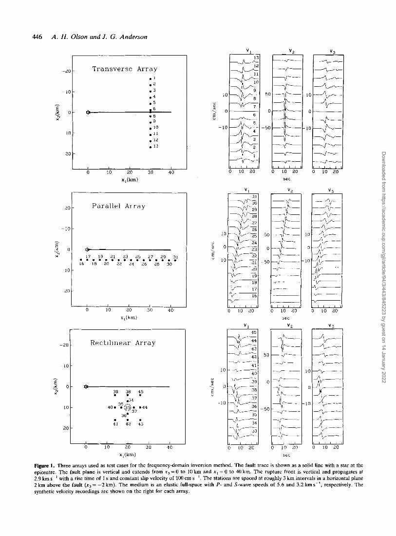
The frequency-domain inversion method was applied to three synthetic data sets generated using Haskell’s (1969) model of a propagating dislocation in a homogeneous elastic fullspace. Figure 1 illustrates the three recording array geometries and the corresponding data that were used in each inversion. Between 13 and 16 stations were used in each case, with average station spacings of 3 km. A vertical fault 10 km wide and 40 km long was located 2 km below the horizontal plane containing the arrays. The slip initiated at the end of the fault is marked with a star in Fig. 1, and propagated as a vertical rupture front at a velocity of 2.9 km s-’. Each point on the fault experienced a constant right-lateral horizontal slip velocity of 100 cm s-l for a duration of l s , delayed by the appropriate rupture time. The P- and S-wave velocities were 5.6 and 3.2kms-l, respectively.

A 200 by 50 grid was used for the discretization (equation 4) resulting in a spacing of 0.2 km on the fault. To test the accuracy of the discretization and the computer implemen- tation of the representation theorem (4), the data in Fig. 1 were calculated as time series with an independent FORTRAN program due to Boatwright & Boore (1975). The discrete Fourier transforms of the data were then computed and compared with their predicted spectral amplitudes using the discrete matrix equation (5). A total of 65 equally-spaced frequency values from 0 to 2.5Hz were used, with the discretization error observed to increase with frequency as expected. A maximum error of a few per cent occurred at 2.5 Hz, where the smallest S-wavelength along the fault (1.28km) was greater than six times the grid spacing.

The number of data at each frequency was between 39 and 48 (three components per station), while the number of complex slip amplitudes to be determined was 20000 (two components of slip at each point). The matrix is clearly singular, reflecting the true non-uniqueness of the problem, and demonstrates the need for a generalized inverse of A ,

Dow



446 A. H . Olson and J . G. Anderson

31 w * fg 20

w 19 w 18

2/ 17

2/ 16 7

I I I I L

10 20

-20

-10

h

E 2 0 x"

10

20

-2c

1c

E 3 0

?1 X

10

20

-20

- 10

- E 5 0 x"

10

20

10

I I I 1 I

0 10 20 30 40

x,(km)

A - q

Parallel Array

0

-10 - ++ J I I I I L

v

17 19 21 29 31 . . . rn . . . t3. t5. <7. . . . 16 18 20 22 24 26 28 30

50

0

-50

I I I I I

0 10 20 30 40

x , h )

__/___

---/------

--

- E- - - ?s-- I I I I I L

Rectilinear Array

-e 3p 3.8 4.5

034 40. 3.5@. 0 4 4

37 36. . . .

41 42 43

I I , I I

0 10 20 30 40

x , ( W

10

0 m

- r l o E

-10

10

0

g o \

- 10 E

10

-1c

u 10 20

v ,

sec

V,

V l

- 40

w I 10 20

sec

sec

c

+ 10

V

7

V

J I I I I I

0 10 20

Figure 1. Three arrays used as test cases for the frequency-domain inversion method. The fault trace is shown as a solid line with a star at the epicentre. The fault plane is vertical and extends from x g = 0 to 10 km and x1 = 0 to 40 km. The rupture front is vertical and propagates at 2.9 km sC1 with a rise time of 1 s and constant slip velocity of 100 cm s-'. The stations are spaced at roughly 3 km intervals in a horizontal plane 2 km above the fault (xg = -2 km). The medium is an elastic full-space with P- and S-wave speeds of 5.6 and 3.2 km s-', respectively. The synthetic velocity recordings are shown on the right for each array.

Dow




such as that produced by the minimum norm condition. It is important to note that the equivalent time-domain inversion would require that all 1 300 000 parameters (65 x 20 000) and 2535-3120 data be inverted simultaneously; such a matrix would require over 3 billion words (complex) of computer storage, hardly practical on even the most sophisticated computer facilities. The ability to decompose the problem with the frequency-domain formulation is therefore essential.

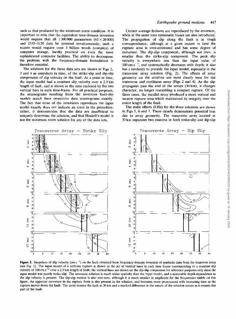
The solutions for the three data sets are shown in Figs 2, 3 and 4 as snapshots in time, of the strike-slip and dip-slip components of slip velocity on the fault. At a point in time, the input model had a constant slip velocity over a 2.9 km length of fault, and is shown as the area enclosed by the two vertical bars in each time-frame. For all practical purposes, the seismograms resulting from the inversion fault-slip models match their resepctive data seismograms exactly. The fact that none of the inversions reproduces the input model exactly does not indicate an error in the procedure; rather, it demonstrates that the data are insufficient to uniquely determine the solution, and that Haskell's model is not the minimum norm solution for any of the data sets.

0 al m

N

0 tl

d

0 m

(0

0 al

m

0

v)

0 3

0

v1

2

Transverse Array - Strike Slip

.- 0 5 10 15 20 25 30 35 4 0

Certain average features are reproduced by the inversion, while at the same time systematic biases are also introduced. The propagation of slip along the fault is in rough correspondence, although at a given instant in time the rupture area is over-estimated and has some degree of curvature. The dip-slip component, although not zero, is smaller than the strike-slip component. The peak slip velocity is everywhere less than the input value of 100 cm s-', and systematically decreases with depth; it also has a tendency to precede the input model, especially in the transverse array solution (Fig. 2). The effects of array geometry on the solution are most clearly seen for the transverse and rectilinear array (Figs 2 and 4). As the slip propagates past the end of the arrays (30 km), it changes character, no longer resembling a compact rupture. Of the three cases, the parallel array produced a more vertical and narrow rupture area which maintained its integrity over the entire length of the fault.

The static offsets (0 Hz) for the three solutions are shown in Figs 5, 6 and 7. These clearly demonstrate potential bias due to array geometry. The transverse array located at 30 km separates two maxima in both strike-slip and dip-slip

Transverse Array - Dip Slip

3

N 6 4 10 !! 0 5 10 15 20 25 30 35 40

Figure 2. Snapshots of slip velocity (cm s-l) on the fault obtained from frequency-domain inversion of synthetic data from the tranverse array (see Fig. 1). The input model of a uniform rupture is shown as the set of vertical lines in each time frame corresponding to a constant slip velocity of 100 cm s-l over a 2.9 km length of fault; the vertical lines are shown on the dip-slip component for reference purposes only since the input model was purely strike-slip. The inversion solution is much wider spatially than the input model, and a noticeable depth-dependence to the slip velocity is present. The dip-slip motion is also non-zero, although it is much smaller in amplitude for the frequencies visible on this figure. An apparent curvature in the rupture front is also present in the solution, and becomes more pronounced with increasing time as the rupture moves down the fault. The array crosses the fault at 30 km and a marked difference in the nature of the solution occurs as it crosses this part of the fault.

Dow



448

0 al

N

0 v1

-?

U

v)

W

0 v)

m

0

(0

52

0 a

2

A . H. Olson and J . G. Anderson

Parallel Array - Strike Slip 0

2 4

6

6

10

2 4

6

8

10

2 4

6

6

10

2 4

6

6

10

2

4

6

a 10

2 4

6

6 ,n L"

0 5 10 15 20 25 30 35 40

Parallel Array - Dip Slip

N 6 d 10 !! 0 5 10 15 20 25 30 35 40

Figure 3. (Analogous to Fig. 2) Snapshots of slip velocity (cms-') on the fault obtained from frequency-domain inversion of synthetic dat: from the parallel array (see Fig. 1) . Although still wider than the input model, the location of rupture in this solution is narrower and more vertical than the solution obtained from the transverse array data (Fig. 21, and the dip-slip component is substantially reduced. A large depth dependence remains in the peak slip velocity of the solution, ranging from 120 cm s-' at the top of the fault to 30 or 40 cm sC1 at the bottom.

offset (Fig. 5). The parallel array, spanning most of the fault length, shows very little horizontal dependence (Fig. 6) , and successfully rules out dip-slip offset. The rectilinear array places most of the slip in the centre of the fault (Fig. 7), reflecting the centralized location of that array. All three solutions show a general decrease of offset with depth, while overestimating the offset in some regions of the fault and underestimating it in others. This is in contrast to the peak slip velocity which is consistently underestimated (Figs

Figures 8-13 show details of the slip-velocity time functions and their corresponding Fourier spectra for a line of points along the centre of the fault. As was apparent in the time-domain snapshots for the transverse and rectilinear arrays solutions (Figs 2 and 4), the time dependence of slip changes character as the rupture passes the end of the arrays at 30 km (Figs 8 and 12). The duration of slip increases and the horizontal propagation velocity of slip onset also increases. In contrast, the time functions for the parallel array solution (Fig. 10) are very similar, with perhaps a small lengthening near the end of the fault. In all cases however, the width of the time function is longer than the input model value of 1.0s. This is evident in the velocity spectra plots (Figs 9, 11 and 13), which show that the

2-4).

source spectral values derived through inversion are much less than the input (solid line), especially at the higher frequencies. The inversion results also have a much faster spectral fall-off than the input model, f - 3 compared to f-'. There is also a tendency for the spectral amplitudes to decrease with distance from the epicentre. These phenom- ena are entirely an artifact of the minimum-norm condition, since non-uniqueness is resolved by finding the model with the smallest rms value of slip velocity integrated over the fault. This condition is required at each frequency, resulting in a solution having the lowest possible average velocity spectra consistent with the data.

The minimum-norm solution is an end member of the set of all models consistent with the data. Although the physical reasonableness of the minimum-norm condition may be debated, it nevertheless provides a useful tool for examining the inherent trade-offs in the inverse problem. Minimization of the rms spectral values must be compensated by changing some other aspect of the solution in order to restore the high-frequency motions recorded on the arrays. A likely candidate for this trade-off is the local phase velocity of slip propagation on the fault. A slip model which propagates toward an array results in the recording of more high frequencies than one which propagates away from the

Dow




Rectilinear Array - Strike Slip Rectilinear Array - Dip Slip

2 -

10-

." 0 5 10 15 20 25 30 35 40

0 ,

f3 10 ii 0 5 10 15 20 25 30 35 40

x 4 -

f3 6 -

2

40

Figure 4. (Analogous to Figs 2 and 3.) Snapshots of slip velocity (cm sC1) on the fault obtained from frequency-domain inversion of synthetic data from the rectilinear array (see Fig. 1). A small amount of curvature to the rupture is visible, though not as pronounced as for the transverse array (Fig. 2). The width of the rupturing area is larger than for the parallel array (Fig. 3), and also exhibits significant depth dependence. As with the transverse array, the solution changes character as the rupture passes the end of the array at 30 km.

'Transverse Array (00 H z )

0 5 10 15 20 25 30 35 40

Parallel Array (0 0 Hz)

0 5 10 15 20 25 30 35 40

L U 0 5 10 15 20 25 30 35 40

Figure 5. Static slip solution (0 Hz) from frequency-domain inversion of synthetic data from the transverse array (see Fig. 1). The input model was a uniform 100 cm in strike-slip offset and 0 cm in dip-slip. The array crosses the fault at 30 km. It is clear that features in the static solution are due entirely to array geometry, thus demonstrating inherent trade-offs in the problem, even at low frequency.

0 5 10 15 20 25 30 35 40

Figure 6. Static slip solution (0 Hz) from frequency-domain inversion of synthetic data from the parallel array (see Fig. 1). The input model was a uniform 100cm in strike-slip offset and Ocrn in dip-slip. This solution very effectively rules out the dip-slip component of slip except at the very ends of the fault. The depth dependence however is clearly not well resolved.

Dow



450 A . H . Olson and J . G. Anderson

Rectilinear Array (0 0 Hz)

0 5 10 15 20 25 30 35 40

Figure 7. Static slip solution (0 Hz) from frequency-domain inversion of synthetic data from the rectilinear array (see Fig. 1). The input model was a uniform 100 cm in strike-slip offset and 0 cm in dip-slip. This solution, although not uniform, is more nearly constant than those for the transverse and parallel arrays (Figs. 5 and 6).

array - the well known phenomenon of seismic focusing. This relative enhancement of high frequencies is independent of the spectral content of slip on the fault.

To estimate the phase velocity at point $ = x and

1400

1200

1000

800 0 a, m \ E u 600

400

200

0

Transverse Array -~ Slip Velocity ~

x 1 = 40

x1 = 36

- , n, x1 = 32

x1 = 28

x1 = 24

x, = 20

X, = 16

x1 = 12

X, = a

x, = 4

x, = 0 . 1 1 , I ,

0 5 10 15 20 25 Sec

Figure 8. Slip-velocity time histories obtained from frequency- domain inversion of synthetic data from the transverse array (see Fig. 1). The box-car functions correspond to the input slip model used to generate the synthetic data. The time functions are shown for the midline of the fault ( x g = 5 km) at a sequence of distances (xl) from 0 to 40 km measured from the epicentre. The corresponding snapshots of slip velocity are shown in Fig. 2. As is also apparent in Fig. 2, the behaviour of the solution changes as the rupture passes the array at 30 km.

frequency f , the following Fourier transform of the slip velocity vector is used.

In (7), E1(x) and E3(x) define local coordinate axes centred at x, and form a plane tangent to the fault surface there. For the planar fault geometry in Fig. 1, these coordinates align with the global x1 (horizontal) and x3 (depth) axes. The x dependence of the transform also enters through the window function, w, which is unity at 5 = x , and smoothly decreases to zero within a specified distance. The space-time dependence of the slip vector in the neighbourhood of x is then obtained by the inverse transform

Negative-phase slownesses (reciprocal of phase velocity), -kJf and -k3/f in (8), correspond to plane-wave components of slip propagating in the positive 5, and E3 directions.

The transforms (7) of the three array solutions are shown in Figs 14-19 for 0.5 and 1.5Hz. In each figure, four 10 x 10 km2 segments along the length of the fault have been transformed. A cosine-square spatial window was applied between the circles 5 < r < 10 km, about the centre of each square. Although the window specification is somewhat arbitrary, it must be larger than the S- wavelength. The Green’s functions (and hence the solutions) contain wavelengths larger than this value, and smaller windows would not be able to resolve their details. Two concentric circles at the P-wave (inner) and S-wave (outer) slownesses are also shown in each transform for reference. The input model had a constant, purely horizontal, rupture velocity of 2.9 km sK1 (0.345 s1km-l) and is shown in Figs. 14-19 by a star just outside the S-wave slowness circle at (kJ f = -0.345, k3/f = 0).

The slowness amplitudes for the transverse array solution (Fig. 14) agree well with the input model at 0.5 Hz for the 0-10 and 10-20 km segments of the fault. Slownesses are nearly horizontal at k l / f = -0.345, with a much larger strike-slip (upper) than dip-slip (lower) component. However, the slowness maximum changes to dip-slip in the 20-30 km segment, and rotates to indicate a more vertically propagating slip vector. In the 30-40km segment, the slowness maximum returns to strike-slip and rotates even further, corresponding to propagation which is vertical and back toward the array. The same rotation is seen in the transforms for 1.5 Hz (Fig. 15), where the slowness contours appear more closely spaced due to the f normalization of the slowness axes, and a secondary maximum has emerged near the P-wave slowness. The rotation in slowness is also observable in the time-domain snapshots (Fig. 2), as the slip-velocity contours become more horizontal when slip occurs beneath the array at 10 s.

Dow




Transverse Array - Slip Velocity

1 o2

l o 1

1 oo E u

lo- '

10-2

10-3 I I 1 I I I I I I I I l l l l l

10-1 100 Hz

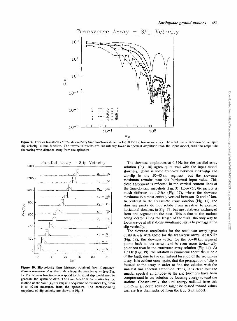
Figure 9. Fourier transforms of the slip-velocity time functions shown in Fig. 8 for the transverse array. The solid line is transform of the input slip velocity, a sinc function. The inversion results are consistently lower in spectral amplitude than the input model, with the amplitude decreasing with distance away from the epicentre.

1400

1 ZOO

1000

800 0 aJ v) \ E o 600

400

zoo

0

Parallel Array - Slip Velocity

-- - X, = 40

x 1 = 36

X , = 32

x 1 = 28

x 1 = 24

X I = 20

X, = 16

x 1 = 12

X I = 8

1 , I

0 5 10 15 20 25 Sec

Figure 10. Slip-velocity time histories obtained from frequency- domain inversion of synthetic data from the parallel array (see Fig. 1). The box-car functions correspond to the input slip model used to generate the synthetic data. The time functions are shown for the midline of the fault (x3 = 5 km) at a sequence of distances (xJ from 0 to 40km measured from the epicentre. The corresponding snapshots of slip velocity are shown in Fig. 3.

The slowness amplitudes at 0.5 Hz for the parallel array solution (Fig. 16) agree quite well with the input model slowness. There is some trade-off between strike-slip and dip-slip in the 30-40 km segment, but the slowness maximum remains near the horizontal input value. This close agreement is reflected in the vertical contour lines of the time-domain snapshots (Fig. 3). However, the picture is much different at 1.5Hz (Fig. 17), where the slowness maximum is almost entirely vertical between 10 and 40 km. In contrast to the transverse array solution (Fig. 15), the slowness peaks do not rotate from negative to positive horizontal slowness in Fig. 17, but are relatively unchanged from one segment to the next. This is due to the stations being located along the length of the fault; the only way to focus waves at all stations simultaneously is to propagate the slip vertically.

The slowness amplitudes for the rectilinear array agree qualitatively with those for the transverse array. At 0.5Hz (Fig. 18), the slowness vector for the 30-40km segment points back to the array, and is even more horizontally polarized than in the transverse array solution (Fig. 14). At 1.5 Hz (Fig. 19), the rotation is symmetric about the middle of the fault, due to the centralized location of the rectilinear array. It is evident once again, that the propagation of slip is focused at the array in order to find the solution with the smallest rms spectral amplitude. Thus, it is clear that the smaller spectral amplitudes in the slip functions have been compensated in the solution by focusing energy toward the stations. Consequently, the total energy radiated from this minimum L, norm solution might be biased toward values that are less than radiated from the true fault model.

Dow



452 A . H. Olson and J. G. Anderson

Parallel Array - Slip Velocity

1 o2

10’

E u

10-1

I 0 --- XI = 4 * --- x, = 12

XI = 20 x --- x, = 28 + _ - -

x1 = 36 * - - _

10-3 I I I I I I I I I I I I I I

10-1 100 Hz

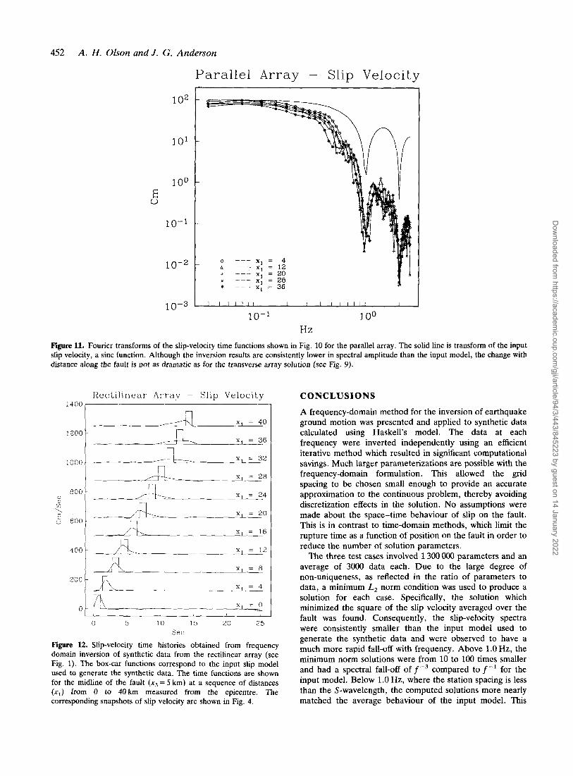
Figure 11. Fourier transforms of the slip-velocity time functions shown in Fig. 10 for the parallel array. The solid line is transform of the input slip velocity, a sinc function. Although the inversion results are consistently lower in spectral amplitude than the input model, the change with distance along the fault is not as dramatic as for the transverse array solution (see Fig. 9).

1400

1200

I000

BOO 0 v’ !E \ E c: 600

-200

200

0

Rectilinear Array - Slip Velocity

x1 = 40

n, , , I X, = 36

X , = 32

x, = 28

x1 = 24

x, = 20

X, = 16

x, = 12

x , = 8

L x 1 = 4

x, = 0 - 1 , 1

0 5 10 15 20 25 Sec

Figure 12. Slip-velocity time histories obtained from frequency domain inversion of synthetic data from the rectilinear array (see Fig. 1). The box-car functions correspond to the input slip model used to generate the synthetic data. The time functions are shown for the midline of the fault (xj = 5 km) at a sequence of distances (x , ) from U to 4Ukm measured from the epicentre. The corresponding snapshots of slip velocity are shown in Fig. 4.

CONCLUSIONS

A frequency-domain method for the inversion of earthquake ground motion was presented and applied to synthetic data calculated using Haskell’s model. The data at each frequency were inverted independently using an efficient iterative method which resulted in significant computational savings. Much larger parameterizations are possible with the frequency-domain formulation. This allowed the grid spacing to be chosen small enough to provide an accurate approximation to the continuous problem, thereby avoiding discretization effects in the solution. No assumptions were made about the space-time behaviour of slip on the fault. This is in contrast to time-domain methods, which limit the rupture time as a function of position on the fault in order to reduce the number of solution parameters.

The three test cases involved 1 300 000 parameters and an average of 3000 data each. Due to the large degree of non-uniqueness, as reflected in the ratio of parameters to data, a minimum L2 norm condition was used to produce a solution for each case. Specifically, the solution which minimized the square of the slip velocity averaged over the fault was found. Consequently, the slip-velocity spectra were consistently smaller than the input model used to generate the synthetic data and were observed to have a much more rapid fall-off with frequency. Above l.OHz, the minimum norm solutions were from 10 to 100 times smaller and had a spectral fall-off of f-’ compared to f-’ for the input model. Below 1.0 Hz, where the station spacing is less than the S-wavelength, the computed solutions more nearly matched the average behaviour of the input model. This

Dow




Rectilinear Array - Slip Velocity

t

0 --- XI = 4 X I = 12 XI = 20

x --- X I = 28

A --- + _ - _

A x1 = 36 * _ - _

I I I I I I l l 1 I

10-1 100 Hz

Figure l3. Fourier transforms of the slip-velocity time functions shown in Fig. 12 for the rectilinear array. The solid line is transform of the input slip velocity, a sinc function. As for the solution to the transverse array data (Fig. 9), the spectral amplitudes decrease with distance from the epicentre and are consistently lower than the input model.

0 - 10 km

-0 4

-0 2

0 2

0 4

Transverse Array - 0 5 Hz

10 - 20 km 20 - 30 km 30 - 40 km

- 0 4 0 0 0 4 - 0 4 0 0 0 4 - 0 4 0 0 0 4 - 0 4 0 0 0 4

k , / f k , / f k l / f k l / f

Figure 14. Spatial wave-number transform of the transverse array solution shown in Fig. 2. The transform is shown for a series of 10 km-square segments along the length of the fault at a frequency of 0.5 Hz. Two concentric reference circles are shown corresponding to the P-wave (inner) and S-wave (outer) slowness, respectively. The combined strike-slip (upper) and dip-slip (lower) transforms for each distance range are normalized to unit peak amplitude, and are contoured at equally-spaced intervals from 0.1 to 1.0, with small and large amplitudes corresponding to dashed and solid lines. The input model had a constant, purely horizontal, rupture velocity of 2.9 km s-' (0.345 s km-') and is shown by a star just outside the S-wave slowness circle at k,/f = -0.345. If the inversion solution resembled the input model, the contours would centre around the star on the strike-slip components and would be zero on the dip-slip. The amplitudes agree well with the input model for the two ranges 0-10 and 10-20 km. However, for the 20-30km range, the motion becomes more dip-slip and the slowness vector changes to become more vertically propagating. At 30-40 km, the motion changes back to strike-slip, with a slowness vector which points vertically up and back toward the centre of the array: this corresponds to propagation back toward the epicentre.

suggests that better resolution at higher frequencies might be achieved if a more dense array of stations were used.

Application of the spatial Fourier transform to the minimum-norm solutions revealed a trade-off between the spectral amplitude of slip at a point on the fault and the local phase velocity of rupture propagation. For each of

Transverse Array - 1 5 Hz

0 - 10 k m 10 - 20 krn 20 - 30 km 30 - 40 km

- 0 4 0 0 0 4 - 0 4 0 0 0 4 - 0 4 0 0 0 4 - 0 4 0 0 0 4

k , / f k l/f k ,/f k l / f

Figure 15. Spatial wave-number transform of the transverse array solution shown in Fig. 2. The transform is shown for a series of 10 km-square segments along the length of the fault at a frequency of 1.5 Hz (see Fig. 14 for other details). The slowness contours are much closer than for 0.5 Hz (see Fig. 14) due to thefnormalization. A clear trend is apparent in which the direction of the slowness vector along the fault points back toward the centre of the array which is at 30km. Spectral amplitudes removed from the slip velocity by the inversion (see Fig. 9) are restored at the array by constructing a rupture which propagates toward the array. This demonstrates a fundamental trade-off, which worsens at high frequency, between the slip function on the fault and the mode of rupture propagation.

Dow



454 A . H . Olson and J . G . Anderson

Rectilinear Array - 0 5 Hi! Parallel Array ~ 0 5 Hz

0 ~ 10 km 30 - 40 km 30 - 40 km 20 - 30 km 10 - 20 km

- . \ .

.- , a ,

-. . . - 0 4 0 0 0 4

10 - 20 km

-0

-0

b y o

0

a - 0

W 1 .- L c

fn

a

a - cn

0

- 0 4 0 0 0 4

a - fn

W 1 - L c

fn

-04 00 0 4 - 0 4 0 0 0 4 -04 0 0 0 4 - 0 4 0 0 0 4

k ,/f k , / f k ,/f , / f

-04 0 0 0 4

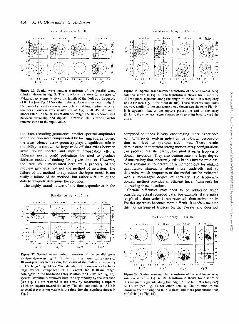
Figure 16. Spatial wave-number transform of the parallel array solution shown in Fig. 3. The transform is shown for a series of 10 km-square segments along the length of the fault at a frequency of 0.5 Hz (see Fig. 14 for other details). As is also evident in Fig. 3, the parallel array does a very good job of matching rupture velocity; the peak slowness very nearly lies at k J f = -0.345, the input model value. In the 30-40 km distance range, the slip becomes split between strike-slip and dip-slip; however, the slowness vector remains close to the input value.

Figure 18. Spatial wave-number transform of the rectilinear array solution shown in Fig. 4. The transform is shown for a series of 10 km-square segments along the length of the fault at a frequency of 0.5 Hz (see Fig. 14 for other details). These slowness amplitudes are very similar to the transverse array slownesses shown in Fig. 14. It is apparent that as the rupture passes the end of the array (30 km), the slowness vector rotates so as to point back toward the array.

the three recording geometries, smaller spectral amplitudes in the solution were compensated by focusing energy toward the array. Hence, array geometry plays a significant role in the ability to resolve the large trade-off that exists between actual source spectra and rupture propagation effects. Different norms could potentially be used to produce different models of faulting for a given data set. However, the trade-offs demonstrated here are a property of the problem geometry and not the method of inversion. The failure of the method to reproduce the input model is not really a failure of the method, but rather a failure of the data to uniquely determine the solution.

The highly causal nature of the time dependence in the

computed solutions is very encouraging, since experience with time series analysis indicates that Fourier deconvolution can lead to spurious side lobes. These results demonstrate that current strong motion array configurations can produce realistic earthquake models using frequency- domain inversion. They also demonstrate the large degree of uncertainty that inherently exists in this inverse problem. What remains is to determine a methodology for making quantitative statements about these trade-offs and to determine which properties of the model can be estimated with a meaningful degree of certainty. The frequency- domain method provides an efficient linear framework for addressing these questions.

Certain difficulties may need to be addressed when considering actual recorded data. For example, if the entire length of a time series is not recorded, then estimating its Fourier spectrum becomes more difficult. It is often the case than an instrument triggers on the S-wave and does not

Parallel Array - 1 5 Hz

0 ~ 10 km 10 - 20 km 20 ~ 30 k m 30 - 40 k m

-0 4

-0 2

% 0 0

* 0 2

0 4

Rectilinear Array - 1 5 Hi!

0 ~ 10 k m 10 - 20 krn m

30 - 40 k m 2.0 - 30 km +I ~ . ~- ,

1 4 0 0 0 4

k , / f

a a

- cn - n

- 0 4 0 0 0 4

r cn L

u - 0 4 00 0 4 - 0 4 0 0 0 4 ' k ,if k l i f k I / f k I / f

Figure 17. Spatial wave-number transform of the parallel array solution shown in Fig. 3. The transform is shown for a series of 10 km-square segments along the length of the fault at a frequency of 1.5 Hz (see Fig. 14 for other details). The slowness vector has a large vertical component in all except the 0-1Okm range. Analogous to the transverse array solution for 1.5 Hz (see Fig. 15), spectral amplitudes removed from the slip velocity by the inversion (see Fig. 11) are restored at the array by constructing a rupture which propagates toward the array. The slip amplitude at 1.5 Hz is so small that it is not visible in the time-domain snapshots shown in Fig. 3.

- 0 4 0 0 0 4

k l / f

- 0 4 0 0 0 4

k ,/f

Figure 19. Spatial wave-number transform of the rectilinear array solution shown in Fig. 4. The transform is shown for a series of 10 km-square segments along the length of the fault at a frequency of 1.5Hz (see Fig. 14 for other details). The rotation of the slowness vector along the fault is clear, and more pronounced than at 0.5 Hz (see Fig. 18).

Dow




include the initial P-wave motions. A n FlT of such a windowed time series produces a frequency series that is a convolution of the unwindowed frequency series. For example, a box-car window in the time domain implies convolution with a sinc function in the frequency domain. This convolution means a coupling of adjacent frequency values, which in turn means that the solution at each frequency cannot be computed independently. However, the degree of coupling will be small if most of the seismogram is recorded. A positivity constraint on the time dependence of slip o n the fault also leads t o frequency coupling, as will most other time-dependent constraints. A s long as the degree of coupling is small, the matrix to be inverted will be block-diagonally dominant and effectively very sparse. This is still a very desirable matrix structure from a computational point of view.

ACKNOWLEDGMENTS

We thank David Boore for providing a F O R T R A N program based upon the Boatwright & Boore (1975) method of computing ground motion for Haskell’s model. This research was supported by the National Science Foundation (NSF) under grants EAR-8418331 and CEE-8319620. Computations were performed on the C R A Y X-MP/48 a t the San Diego Supercomputer Centre (SDSC), through grants made available by the NSF and SDSC.

REFERENCES

Aki, K. & Richards, P. G., 1980. Quantitative Seismology - Theory and Methods, Vol. 1, W. H. Freeman, San Francisco.

Anderson, J. G. & Trifunac, M. D., 1977. Current computational methods in studies of earthquake source mechanisms and strong ground motion, in Proc. Symp. Applications of Computer Methods in Engineering, Vol. 2, ed. Wellford, L. Carter, University of Southern California.

Archuleta, R. A., 1984. A faulting model for the 1979 Imperial Valley earthquake, J . geophys. Res., 89, 4559-4585.

Backus, G. & Gilbert, F., 1970. Uniqueness in the inversion of inaccurate gross earth data, Phil. Trans. R. SOC., 266, 123-192.

Bergland, G. D., 1969. A guided tour of the fast Fourier transform, IEEE Spectrum, 6, 41-52.

Beroza, G. C. & Spudich, P., 1987. Heterogeneous fault rupture inferred from high frequency near-source data, XIX General Assembly, Znt. Un. Geodesy and Geophys., Abstr, Vol. 1, p. 338.

Beroza, G. C. & Spudich, P., 1988. Linearized inversion for fault rupture behavior: application to the 1984 Morgan Hill, California earthquake, J. geophys. Res., in press.

Boatwright, J. & Boore, D. M., 1975. A simplification in the calculation of motions near a propagating dislocation, Bull. seism. SOC. Am., 65, 133-138.

Burridge, R. & Knopoff, L., 1964. Body force equivalents for seismic dislocations, Bull. seism. SOC. Am., 54, 1875-1888.

Gilbert, F., 1971. Ranking and winnowing gross earth data for inversion and resolution, Geophys. J. R. astr. SOC., 23,

Hartzell, S. H. & Heaton, T. H., 1983. Inversion of strong ground motion and teleseismic waveform data for the fault rupture history of the 1979 Imperial Valley, California, earthquake, Bull. seism. SOC. Am., 73, 1553-1583.

Hartzell, S. H. & Helmberger, D. V., 1982. Strong-motion modelling of the Imperial Valley earthquake of 1979, Bull. seism. SOC. Am., 72, 571-596.

Haskell, N. A., 1969. Elastic displacements in the near-field of a propagating fault, Bull. seism. SOC. Am., 59, 865-908.

Jackson, D. D., 1972. Interpretation of inaccurate, insufficient, and inconsistent data, Geophys. J . R. astr. Soc., 28, 97-109.

Olson, A. H. & Apsel, R. J., 1982. Finite faults and inverse theory with applications to the 1979 Imperial Valley earthquake, Bull. seism. SOC. Am., 72, 1969-2001.

Olson, A, , 1987. A Chebyshev condition for accelerating convergence of iterative tomographic methods - solving large, least squares problems, Phys. Earth Planet. Int., 47, 333-345.

Spudich, P. K. P., 1980. The Dehoop-Knopoff representation theorem as a linear inverse problem, Geophys. Res. Lett., 9,

Wiggins, R., 1972. The general linear inverse problem: implications of surface waves and free oscillations on earth structure, Rev. Geophys. Space Phys., 10, 251-285.

Yoshida, S., 1986. A method of waveform inversion for earthquake rupture process, J. Phys. Earth, 34,235-255.

125-128.

717-720.

Dow



implications of frequency-domain inversion of earthquake ground

Documents