impact of transport models on connectivity of …

Impact of Transport Models on Connectivity of Vehicular Ad-hoc Networks HO, Ivan; NORTH, Robin; POLAK, John; LEUNG, Kin

12th WCTR, July 11-15, 2010 – Lisbon, Portugal

1

Ivan Wang-Hei Ho, Department of Electrical and Electronic Engineering, Imperial College London, [email protected]

Robin J. North, Centre for Transport Studies, Imperial College London, [email protected]

John W. Polak, Centre for Transport Studies, Imperial College London, [email protected]

Kin K. Leung, Department of Electrical and Electronic Engineering, Imperial College London, [email protected]

ABSTRACT

Vehicular Ad-Hoc Networks (VANETs) are attracting considerable research and commercial interest with promising applications in a number of areas including cooperative vehicle-highways systems, sensor networks and safety systems. However, due to high speed and variable driver behaviour, automotive ad-hoc networks will behave in fundamentally different ways to the most prevalent models in Mobile Ad-Hoc Network (MANET) research. Previous work in MANETs usually assumes that the mobile nodes move randomly with an unconstrained mobility model and it is clear that a random mobility model is not adequate to represent the major characteristics of real-world vehicle motions, and may therefore lead to unreliable results. Recent studies of VANETs have attempted to introduce macro- and micro-mobility constraints to model vehicle motions, but they usually focus on modelling the mobility of generic private vehicles. Given the potential for the co-ordinated deployment of network nodes on centrally-managed fleet vehicles, it has become important to model the characteristics of a VANET featuring vehicles of different types, with systematically different behaviour patterns. In this paper, we study the connectivity of mobile ad-hoc networks that consist of buses moving in urban area, and examine the implications for transport-related services. Buses have a unique set of behaviour characteristics, such as fixed routes, schedules, bus stops, specific priorities, etc., which gives rise to distinct impact on node connectivity in the communication network. Through extensive simulations based on real bus routes in central London, we demonstrate the impact of the locations of stops and the prevailing traffic patterns on node connectivity (including the distributions of contact duration and inter-contact time between buses), and explore its implication on the design of a dissemination system to capture and disseminate data. Our results give a key message that

IMPACT OF TRANSPORT MODELS ON CONNECTIVITY OF VEHICULAR AD-HOC

NETWORKS



2

the mobility of buses has to be modelled explicitly, and such kind of knowledge of connectivity among buses will be significant for the studies of routing algorithms and other networking functions in inter-bus communication networks.

1. INTRODUCTION

Vehicular Ad-Hoc Networks (VANETs), a subclass of Mobile Ad-Hoc Networks (MANETs), consist of vehicles moving on urban streets, communicating with each other wirelessly in the absence of any other communications infrastructure. Due to their readily deployable nature and potential functions in road safety, detecting traffic accidents and incidents and reducing traffic congestion, VANETs are attracting significant attention from the research community. There are a number of previous demonstrations of using existing wireless technology for achieving vehicle-to-vehicle communications in the real world. For instance, Festag et al. (Festag et al., 2004) describe the real-world field trials of a car-to-car communication platform with an IEEE 802.11 air interface, while Bucciol et al. (Bucciol et al., 2005) conducted video streaming experiments between two vehicles moving on highway and urban road networks. These experiments show that existing technology is feasible for building connections between mobile users in cars with intermittent connectivity. VANETs also have applications in the design and operation of sensor networks. An example of an application of this sort is the MESSAGE project which aims to deploy a mobile wireless air quality sensor network on buses in London (Cohen et al., 2007).

However, the constraints associated with vehicle movements, varying driver behaviour, and high speed cause rapid topology changes, frequent fragmentation of the network, and limited utility from network redundancy. These features cause the characteristics of VANETs to differ substantially from traditional, random motion MANET models. These differences also have implications for the VANET architecture, ranging from the physical to application layers in the OSI model for communications and for computer network protocol design.

In general, the impact of mobility on the performance of communication protocols can be described using the block diagram shown in Figure 1. First, different mobility models have different degrees of spatial dependence, temporal dependence, relative speeds and geographic restrictions, which give rise to different (communication) link durations and inter-contact time between nodes, and thus distinct (communication) path availabilities for multi-hop transmissions. Network connectivity in turn influences the performance of the communication protocol. It has been shown that a longer link duration will result in higher throughput (Bai et al., 2003). Therefore, to ensure the design feasibility of VANETs, we require a fundamental understanding of the relationships between vehicular mobility and node connectivity (the first two blocks in Figure 1), which is the focus of this paper.

Much of the previous work in MANETs (Bai et al., 2004; Bai et al., 2003; Cai et al., 2007) has neglected real-world constraints when modelling node mobility. For instance, the popular random waypoint model is widely used in MANET research for the ease of analysis, but assumes that mobile nodes move in an open-field without any obstacles and ignores real-world factors affecting vehicles such as street layouts and inter-vehicle interactions. Clearly, this kind of random mobility model cannot adequately capture the major characteristics of vehicular traffic (the reader can refer to our previous work (Ho et al., 2007) for the comparison of node connectivity of unconstrained random waypoint and road-constrained



3

car-following models), and so there is a necessity to introduce realistic mobility models for VANETs, which is critical for reliable evaluation of the communication system performance.

Figure 1 – Block diagram illustrating the impact of mobility on the performance of communication protocols.

In transport studies, when dealing with vehicular traffic, we usually refer to the marco- and micro-mobility descriptions (Harri et al., 2007) for modelling the driver-to-infrastructure and driver-to-driver interactions respectively. Macroscopic mobility describes gross quantities of interest, such as density or average velocity of vehicles, and considers vehicle movements to be analogous to fluid dynamics; while microscopic mobility treats each vehicle as a unique individual, and more accurately models its behaviour, but with higher computational cost.

There are a number of studies that restrict nodes’ macro-mobility on highway and grid topologies. For example, the Freeway and Manhattan models are described in (Bai et al., 2003), and the authors of (Yang et al., 2005) evaluate through simulation the feasibility of traffic information propagation in freeway and arterial grid networks via information exchange among vehicles. However, these road topologies are rather simple and regular, and many other transport features such as multiple lanes, traffic lights and stop signs are neglected.

Recent VANET research has tried to incorporate various macro- and micro-mobility factors into the models. For instance, Saha et al. (Saha et al., 2004) model vehicle mobility on a real street map from the TIGER database (2009e), however, they do not model any interactions between vehicles, and nor do they include traffic control at road intersections. The Street Random Waypoint (STRAW) Model (Choffnes et al., 2005) introduces traffic control and stop signs at road intersections and the car-following interactions between vehicles moving in an urban grid. Mahajan et al. (Mahajan et al., 2007) then propose several simulation models that account for various urban constraints such as street layout, traffic rules, multi-lane roads, acceleration, RF attenuation due to obstacles, etc. This extends Jardosh et al. (Jardosh et al., 2003), which suggests an obstacle-based mobility model, where the obstacles are used both to define the movement pathways of the mobile nodes and to attenuate radio transmissions.

As an alternative to purely simulation driven analyses, other studies employ real-world mobility traces for evaluating MANET performance (Krumm et al., 2005; Zhang et al., 2007). Although these mobility traces capture real-world vehicle activity, they are case-specific and therefore difficult to generalize as vehicles typically alter their trajectory based on the prevailing traffic conditions.

Nevertheless, when considering these studies as a whole, it appears that none of them considers a mix of mobile nodes attached to different types of vehicles with significantly different mobility patterns, rules, and priorities on the road. For example, generic private cars



4

have no designated routes or fixed origins and destinations, while scheduled transport systems (e.g., buses) have structured mobility patterns with fixed routes and timetables, origins and destinations. Motivated by the requirements of the MESSAGE project, the aim of this paper is to study the impact of various transport factors on connectivity of an inter-bus communication network and explore its communication capability for disseminating pollutant, and other sensor data. Our main contributions in this paper are as follows: • We develop a simulation framework for simulating a semi-realistic inter-bus

communication network in central London and demonstrate the impact of various macroscopic and microscopic transport models on node connectivity. In addition, we study the fundamental properties of the contact duration and inter-contact time between vehicles, which have been critical metrics in MANET research in determining the capacity and routing delay of communication networks. Such findings will provide guidelines on mobility modelling, performance analysis, and protocol design in VANETs.

• We investigate the discrepancies between the connectivity statistics of private vehicles and buses, which show the importance of modelling bus mobility independently. Specifically, we find that multi-hop communication paths have much poorer connectivity statistics than single-hop communication links in the bus network mobility scenario. This raises the issue of the feasibility of multi-hop transmissions for real-time applications in inter-bus communication networks, with implications for the types of services such a network may support.

• We identify the network requirements (e.g., data rate, data latency, etc.) for a set of transport-related data dissemination services and quantify the feasibility of disseminating such data among buses. We explore from both an e-Science and a transport perspective of the impact that the characteristics of the communication network have on the rest of the system design. The rest of the paper is organized as follows. Section 2 presents a transport modelling

framework for realistic VANET simulations, especially for simulating bus movements. Section 3 introduces the set of metrics for evaluating node connectivity in communication networks. Section 4 presents and analyzes the results of the bus network simulations, explores the influences of various transport elements on network connectivity, and studies the distributions of the contact duration and inter-contact time in inter-bus communication networks. Section 5 explores the implication of bus connectivity on the provision of transport-related data services. Finally, Section 6 concludes the paper.

2. A TRANSPORT MODELLING FRAMEWORK FOR REALISTIC SIMULATION OF VANETS

We present in this section a framework which captures both macroscopic and microscopic behaviour characteristics of transport networks to facilitate more realistic study of vehicular communications networks. We identify two major building blocks: mobility constraints and vehicular traffic generation, for modelling real-world vehicular movements (see Figure 2). The following subsections describe these blocks and their components.



5

Figure 2 – Transport modelling framework for realistic vehicular network simulation.

2.1. Mobility Constraints

The mobility constraints define the relative degree of freedom of vehicle movements. Macroscopically, the vehicle is constrained by the road network topology, per-road characteristics and obstacles (e.g. road capacity, speed limits); while microscopically, it is influenced by neighbouring vehicles and the driver’s behaviour in relation to them;

1. Road Network: The motion of vehicle is restricted to the geometry of the road topology. The road network contains different categories of streets, multiple lanes, and each road segment is associated with a speed limit, which restricts the velocity of the leading vehicle and thus the following cars on the road. Moreover, traffic lights are located at road junctions. These act as gates on the road and cause bunching of vehicles, while at the same time, separating vehicles into clusters, or “platoons”. Therefore, traffic lights may be expected to have a strong impact on the node connectivity of communication network.

2. Neighbouring Vehicles: Unlike generic mobile nodes in MANET simulations, real vehicles cannot pass through a space already occupied by another vehicle. Instead, neighbouring vehicles influence one another, with their inter-dependent motion being defined by their individual driving behaviour. Two classes of interactions are specifically modelled; Acceleration Models: Two groups of acceleration model are necessary: car-following models, which describe the acceleration drivers apply in reaction to the behaviour of the vehicle in front, and general acceleration models, which apply when drivers do not closely follow their leaders. A car-following model adapts a following car’s mobility according to a set of rules in order to maintain a safe distance and avoid collision with the lead vehicles and a number of alternative formulations exist including Psycho-Physical Models, Linear Models, Cellular Automata, and Fuzzy Logic Models (Brackstone et al., 1999). Lane-changing Models: Modelling lane-changing behaviour is a more complex task. It mainly consists of two steps: the lane-selection process (the decision to consider a lane change and the lane choice) and the decision to execute the lane change. Lane



6

changes are either mandatory (MLC) or discretionary (DLC). MLC are executed when driver must leave the current lane. DLC are executed to improve driving condition. Gap-acceptance models are used to model the execution of lane changes. Some widely used models in transport studies include the Gipps Model (Gipps, 1986) and Wiedemann Psycho-Physical Model (Wiedemann, 1991) for lane changing.

2.2. Vehicular Traffic Generation

These models are responsible at a macroscopic level for generating traffic flows consisting of different types of vehicles. In our simulations, we consider two types of vehicles: buses and generic private vehicles. The vehicular traffic generation model is then used to define the traffic flow and the vehicle density based on overall network considerations. It then considers the characteristics of vehicles according to their types, and assigns them with different traffic patterns, rules and priority.

Every vehicle in the network has an origin and a destination. The position may be either random, random restricted on a graph or based on a set of attraction points. After having defined the start and end points, a trip, which consists of a list of waypoints, may be generated randomly, with pre-defined routes, or with algorithms such as Dijsktra’s Algorithm between the points. In this paper, two different traffic generation models are used;

1. Bus Traffic Generation: Buses have fixed origins and destinations, and pre-defined bus routes and timetables. While en route, the bus stops at bus stops to load and unload passengers. In our simulation, we generate bus traffic based on real bus route data provided by London Buses. Specifically, we acquire the list of waypoints which define the bus routes, and specific positions of bus stops along the routes. In London, measures are taken to reduce the impact of congested traffic on bus operations through the creation of bus-only lanes. Traffic lights cause bunching of vehicles, and bunching of buses is not a desirable phenomenon, especially from the perspective of bus passengers. To combat this, bus priority measures are installed at numerous junctions in London to aid in reducing delay and in regulating the headway between buses on the same route. There are also many roads along which multiple bus routes operate and interact. All of these network characteristics combine to affect the spatial density of the buses and hence the network connectivity.

2. Background Traffic Generation: Traffic that consists of other, non-communicating vehicles (non-buses) may cause congestion on the road and thus delay the bus journey. In this paper we generate background vehicle traffic with random origins and destinations on the road network, following random walk or sight-seeing trip models to wander around the study region. When a background vehicle passes through a road intersection, it randomly selects a new speed within a user defined range and chooses a direction (e.g., turn left, turn right or go straight) to proceed in. Vehicles may also stop at the intersections due to traffic signals. The vehicle randomly walks until it is a certain distance (e.g. 1 km) from the starting point and then takes the shortest path back to the starting point before it starts again along a different random path. By distributing the origins around the network, this allows a pseudo-realistic distribution of background traffic to be generated.



7

3. NODE CONNECTIVITY METRICS

In this paper we use the node connectivity metrics introduced in (Ho et al., 2007) to evaluate multi-hop connectivity in the simulated bus network. In this section, we re-state these metrics and provide further elaboration of each parameter.

Let X1(i, j, t) be a random variable for indicating the single-hop connectivity between nodes i and j at time t such that it equals 1 when Di,j(t)≤ R, and 0 otherwise, where Di,j(t) denotes the Euclidean distance between nodes i and j at time t, and R is the transmission range of a mobile node.

Generally, we use Xk(n1, nk+1, t) to indicate multi-hop connectivity, where k ≥ 1 is an integer which denotes the number of hops in the communication path { }1 2 1, ,..., kp n n n += ,

between nodes n1 and nk+1. Specifically, Xk(n1, nk+1, t) = 1 if and only if X1(ni, ni+1, t) = 1 {1, 2,..., }i k∀ ∈ ; AND Xi(n1, nk+1, t) = 0 {1, 2,..., 1}i k∀ ∈ − . Otherwise, Xk(n1, nk+1, t) = 0. This

means that nodes n1 and nk+1 are connected with at least one k-hop path at time t, given that they cannot be connected with less than k hops at that time. We then define;

1. Number of Connected Node Pairs (k-hop): We denote this as Pk. It is the number of node pairs (i, j) that have ever been connected with at least one k-hop path throughout the simulation period. Specifically, Pk is the number of node pairs (i, j) such that

0( , ) ( , , ) 0

T

k kt

X i j X i j t=

= >∑ , where T is the total simulation period.

2. Number of Connected Periods (k-hop): The number of connected periods of the k-hop path between a pair of nodes i and j, denoted as CPk(i, j), is the number of times the path status between them changes from ‘down’ to ‘up’. Formally,

0

( , ) ( , , )T

k kt

CP i j C i j t=

= ∑ (1)

where Ck(i, j, t) is an indicator random variable such that Ck(i, j, t) = 1 iff Xk(i, j, t – 1) = 0 and Xk(i, j, t) = 1. That is, if the k-hop path between nodes i and j is down at time t – 1, but comes up at time t then we increment CPk by 1. We also define that Ck(i, j, 0) = 1 if Xk(i, j, 0) = 1. Average Number of Connected Periods (k-hop) is then the average value of CPk(i, j) over the number of k-hop connected node pairs Pk. We have

1 1( , )

N N

ki j i

kk

CP i jCP

P= = +=∑ ∑ (2)

3. Path Duration (k-hop): This is the average duration in time of the k-hop path existing between two nodes i and j. It is a measure of the stability of the path. Formally,

0( , , )

( , )( , )

T

kt

kk

X i j tPD i j

CP i j==∑

(3)

We define PDk(i, j) = 0 if CPk(i, j) = 0. Note that PD1(i, j) represents the single-hop link duration between the node pair (i, j). Average Path Duration (k-hop) is the average value of PDk(i, j) over the number of k-hop connected node pairs Pk. We have



8

1 1( , )

= = +=∑ ∑N N

ki j i

kk

PD i jPD

P (4)

4. Fraction of Connected Time (k-hop): This is the ratio of the total amount of time that a pair of nodes i and j are connected with the k-hop path throughout the simulation period to the amount of time that the two nodes co-exist in the network. Formally,

0( , , )

( , )( , )

T

kt

k

X i j tFT i j

CT i j==∑

(5)

where CT(i, j) denotes the amount of co-existed time of nodes i and j in the network, specifically, it consists of the total connected and disconnected time of the k-hop path between nodes i and j. Therefore, 1 – FTk(i, j) will be the fraction of disconnected time of the k-hop path. Average Fraction of Connected Time (k-hop) is the average value of FTk(i, j) over the number of k-hop connected node pairs Pk. We have

1 1( , )

N N

ki j i

kk

FT i jFT

P= = +=∑ ∑ (6)

Note also that the total connected time of a communication path is equal to the summation of all the connected durations between the two nodes in the simulation. Therefore, a communication path with a shorter average duration does not necessarily mean a smaller fraction of connected time as there could be more number of connections made throughout the simulation period. The combination of these metrics therefore allows us to gain a detailed understanding of the characteristics of the vehicle-based communications network.

4. LONDON BUS NETWORK SIMULATIONS: RESULTS AND ANALYSIS

In this section, we present the results and analysis of the London bus network simulations based on the set of metrics presented in the previous section. A test network was constructed to include the real-world road topology and the actual geometry of three bus routes in the central London area. To demonstrate the importance of general transport models on connectivity studies, we present results of the bus network simulations with different densities of buses (as defined by the operating headway time between adjacent buses), and examine the influences of stop signs and background traffic on node connectivity. Finally, we evaluate the distributions of the contact duration and inter-contact time between buses.

In this paper we focus our discussion on parameters that were observed to have the most significant impacts on node connectivity. It is part of ongoing research to investigate the impact of other traffic phenomena (e.g. bus priority) on vehicular networks in order to understand which elements must be considered and which can be neglected for a reliable evaluation of VANET performance.



9

4.1. Model Configuration

Several simulators including ns-2 (2009c), QualNet (2009d), and OPNET (2009a) have been developed for generic ad-hoc networks and modelling of the wireless channel. However, these do not support specific vehicle network topologies, while road traffic simulation models such as VISSIM (PTV, 2009), Paramics (SIAS, 2009) and SUMO (2009b) provide highly accurate traffic queuing and vehicle interaction models, but do not typically integrate any aspects of inter-vehicle communication.

GrooveNet (Mangharam et al., 2006), jointly developed by Carnegie Mellon University (CMU) and General Motors Corporation, is a hybrid simulator which enables communication between fully simulated vehicles, vehicles following “real” measured trajectories and between combinations of the two. It supports modelling of inter-vehicular communication within a real street map-based topography, and its modular architecture incorporates mobility, trip and message broadcast models over a variety of link and physical layer communication models. Overall, we found that GrooveNet has competitive capability in both the transport and communication aspects, it is therefore used for our simulations with customized modules to output the set of node connectivity metrics.

According to Section 2, there are a number of input parameters for the simulation in order to define the propagation of buses and node density. In general, it includes 1) the geometry of the bus routes and road network; 2) the propagation speeds and characteristics of vehicle types; and 3) the bus headway and density of vehicles. In the followings, we configure these input parameters based on real-world data and statistics.

For the road network (1 above), we focus on studying an inter-bus communication network in central London, centred on Camden Town. We have reconstructed the Camden Town region in the simulator based on road network data obtained from Ordnance Survey, and we acquired real bus route data from London Buses for three bus routes which pass through the region. Specifically, this included the coordinates (in terms of longitude and latitude) of the waypoints of the bus routes and those of the bus stops. The bus routes that we simulate are Routes 27, 31 and 88, with each route being split into two runs to represent the ‘out’ and ‘back’ journeys. Figure 3 shows how the three bus routes intersect with each other geometrically. Figure 4 shows the simulated road network in Camden Town with buses and background vehicles on it.

Figure 3 – Geometry of bus routes 27, 31, and 88 that run through Camden Town, London.



10

Figure 4 – Bus network simulation of Camden Town, London.

For the vehicle types (2 above), we considered buses and generic background vehicles in the simulation. In Figure 4, the solid circles denote buses with communication capability. These follow a bus trip model (based on the real bus routes data) to move from their origins to destinations (bus terminals) with stops at intermediate bus stops. When the background traffic is included, we can see the circle inscribed triangles that denote other vehicles without communication capability. These act as obstacles of the traffic flow of buses, and they use a sightseeing trip model to wander around the region.

The transmission range of buses is fixed to be 200 meters in the simulations unless otherwise specified. All vehicles on the road employ a car-following model (Rothery, 1992), where a vehicle will not exceed the speed of the vehicle in front. A vehicle that is determined to be a leader vehicle will use a general acceleration model. Here, the street speed mobility model is used where vehicles always move within user-defined range of the speed limit of the road.

Table 1 – Real-world statistics and simulated data of the three bus routes.

Route No. Route Length

(mile) Journey Time

(min) Peak Hour Freq. (min)

Avg. Journey Time in Simulation (min)

Average Speed in Simulation (mph)

27 9 47 – 90 7 – 8 58 9.31 31 6 35 – 63 6 47 7.66 88 7 39 – 67 7 – 8 49 8.57

Table 1 shows the basic information of the three simulated bus routes (e.g., length of the route, journey time, and peak hour frequency) according to Transport for London (TfL, 2009b). In the simulations, we configure the street speed mobility model such that the leading speed of buses varies from 9 to 15 mph. With this speed setting, we have the average journey time taken for a bus to finish the whole route consistent with the TfL statistics (TfL, 2009b) as shown in Table 1. Based on the Route length and the average journey time, we can further derive the average speed of buses in the simulations, which is between 7.7 and 9.3 mph, this again is consistent with the average London bus speed that ranges from 6.21 to 9.32 mph according to Figure 5.5 in TfL report (TfL, 2008).



11

Figure 5 – Bus Stop locations in Camden Town, London (TfL, 2009a).

For the bus headway and schedule (3 above), we can see from Table 1 that the peak hour frequency/headway of buses in the three routes ranges from 6 to 8 min. However, since we do not simulate all the bus routes that share the same road portions with the three bus routes, the simulated headway is considered as the ‘aggregated’ headway that captures the combined effect of all the buses operating through the routes, which should be smaller than the scheduled headway (6 to 8 min) of the three routes.

To estimate the aggregated headway and consider the combined effect of all the buses operating through the routes, we examine the number of buses that pass through bus stops X and Y in Camden High Street and bus stops T and U in Bayham Street (as shown in Figure 5) between 08:00 and 10:00 on a weekday morning according to the bus information from Transport for London (TfL, 2009a). For instance, for the link in Camden High Street containing bus stops X and Y, there are 8 routes operating: 24, 27, 29, 31, 134, 168, 214 and 253. In Table 2, we find the number of buses on these routes passing through the link between 08:00 and 10:00 on a weekday morning as being representative of the peak bus density. We then derive the mean aggregated headway for the two links as 1.4 and 1.3 min. Hence, given the variability of on-street arrival times, we have the inter-arrival time of buses in the simulations varies in steps from 30 sec to 5 min, which is reasonable to reflect the aggregated headway of the routes and provides a measure of the VANET performance should all buses be instrumented.

Table 2 – Estimation of the aggregated bus headway. No. of buses pass through bus stops X and Y in

Camden High Street from 08:00 to 10:00 on a weekday No. of buses pass through bus stops T and U in

Bayham Street from 08:00 to 10:00 on a weekday Bus Route No. of buses Bus Route No. of buses

24 22 27 22 27 17 31 20 29 24 88 17 31 20 168 19 134 25 214 17 168 19 253 25 214 17 274 16 253 25 C2 17

Total 169 Total 153 Aggregated Headway (min) 1.4083 Aggregated Headway (min) 1.2750



12

4.2. Performance of Multi-hop Transmission in Bus Network

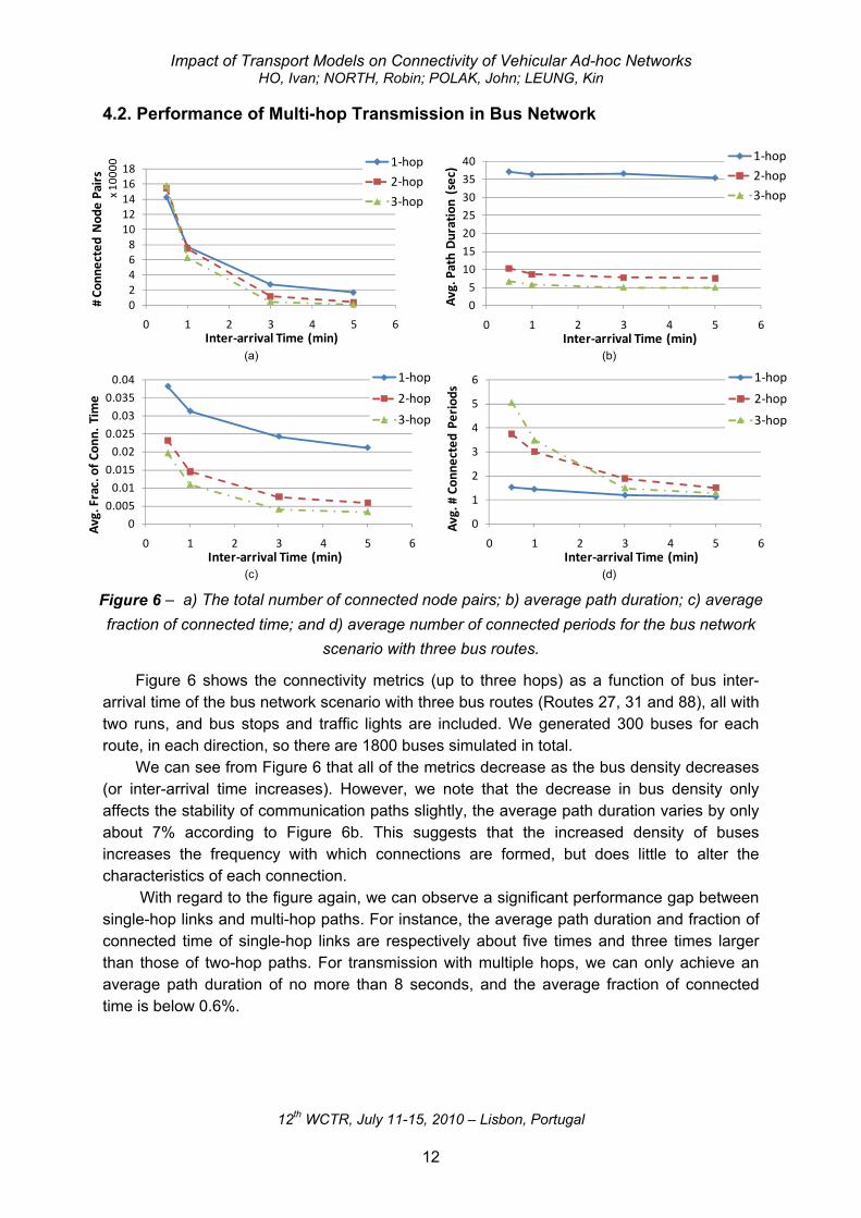
Figure 6 shows the connectivity metrics (up to three hops) as a function of bus inter-arrival time of the bus network scenario with three bus routes (Routes 27, 31 and 88), all with two runs, and bus stops and traffic lights are included. We generated 300 buses for each route, in each direction, so there are 1800 buses simulated in total.

We can see from Figure 6 that all of the metrics decrease as the bus density decreases (or inter-arrival time increases). However, we note that the decrease in bus density only affects the stability of communication paths slightly, the average path duration varies by only about 7% according to Figure 6b. This suggests that the increased density of buses increases the frequency with which connections are formed, but does little to alter the characteristics of each connection.

With regard to the figure again, we can observe a significant performance gap between single-hop links and multi-hop paths. For instance, the average path duration and fraction of connected time of single-hop links are respectively about five times and three times larger than those of two-hop paths. For transmission with multiple hops, we can only achieve an average path duration of no more than 8 seconds, and the average fraction of connected time is below 0.6%.

(a) (b)

(c) (d) Figure 6 – a) The total number of connected node pairs; b) average path duration; c) average fraction of connected time; and d) average number of connected periods for the bus network

scenario with three bus routes.

02468

1012141618

0 1 2 3 4 5 6

# Co

nnected Nod

e Pairs

x 10

000

Inter‐arrival Time (min)

1‐hop

2‐hop

3‐hop

0

5

10

15

20

25

30

35

40

0 1 2 3 4 5 6

Avg. Path Duration (sec)


1‐hop

2‐hop

3‐hop

0

0.005

0.01

0.015

0.02

0.025

0.03

0.035

0.04

0 1 2 3 4 5 6

Avg. Frac. of C

onn. Tim

e


1‐hop

2‐hop

3‐hop

0

1

2

3

4

5

6

0 1 2 3 4 5 6

Avg. # Con

nected

Periods


1‐hop

2‐hop

3‐hop



13

Such poor multi-hop performance can be explained in two ways. First, the existence of two-hop paths requires more constraints to be satisfied than single-hop links, making them less likely to be maintained in the network. For instance, the existence of a single-hop link only requires that the receiver node be within the communication range of the transmitter node, while a two-hop path requires both the transmitter and receiver nodes be within the communication range of the forwarding node, while also requiring that the transmitter and receiver be beyond the direct communication range of each other. Second, and as a consequence, multi-hop performance is more vulnerable to variations in the mobility pattern. Our findings tend to suggest that the bus mobility pattern does not favour multi-hop transmissions. This is in contrast to some other mobility scenarios; for example, an urban mobility model when we consider a communications network formed by all the background vehicles in the Camden Town bus network, in which the private vehicles perform random walks in an urban grid. The reader is referred to Section 2.2 for the detailed description of the generation of private vehicles’ movements. In this case, we find that the fraction of connected time of multi-hop paths is larger than that of single-hop links when the node density is high.

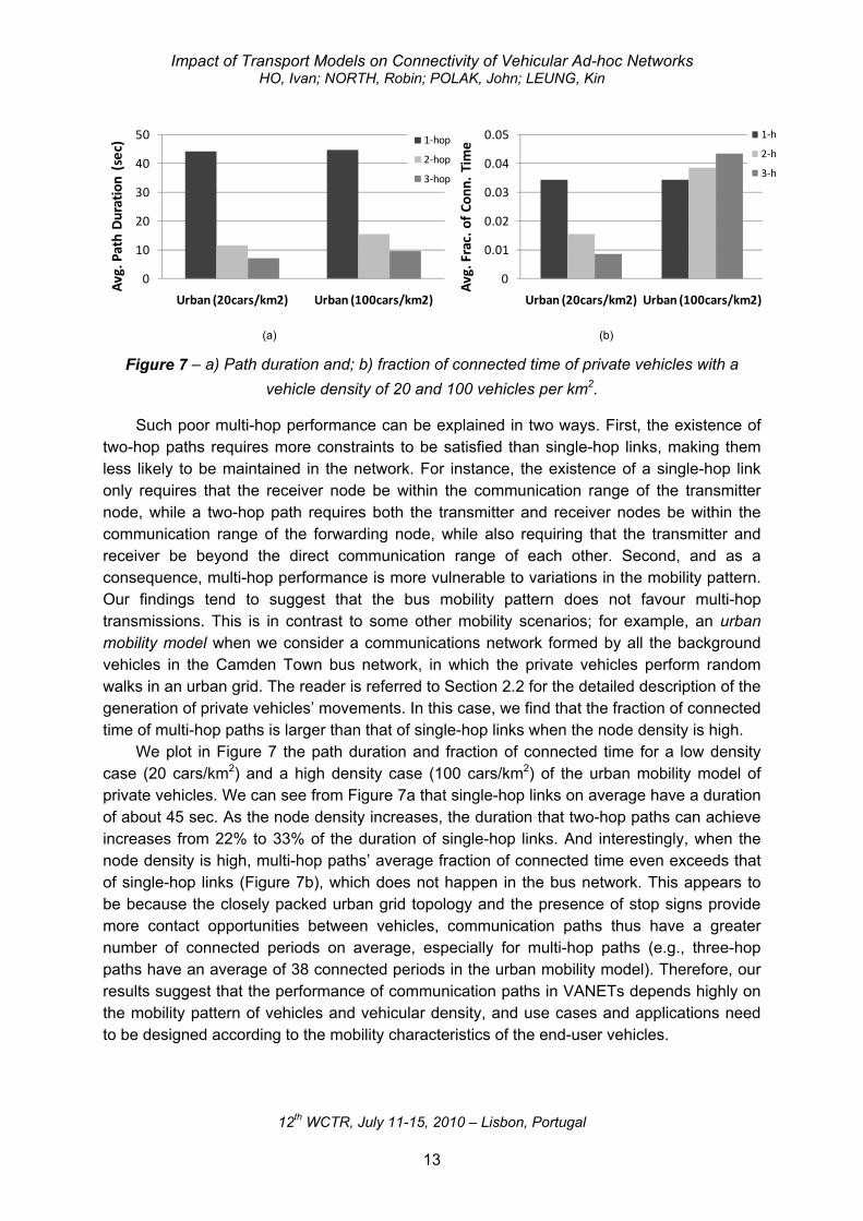
We plot in Figure 7 the path duration and fraction of connected time for a low density case (20 cars/km2) and a high density case (100 cars/km2) of the urban mobility model of private vehicles. We can see from Figure 7a that single-hop links on average have a duration of about 45 sec. As the node density increases, the duration that two-hop paths can achieve increases from 22% to 33% of the duration of single-hop links. And interestingly, when the node density is high, multi-hop paths’ average fraction of connected time even exceeds that of single-hop links (Figure 7b), which does not happen in the bus network. This appears to be because the closely packed urban grid topology and the presence of stop signs provide more contact opportunities between vehicles, communication paths thus have a greater number of connected periods on average, especially for multi-hop paths (e.g., three-hop paths have an average of 38 connected periods in the urban mobility model). Therefore, our results suggest that the performance of communication paths in VANETs depends highly on the mobility pattern of vehicles and vehicular density, and use cases and applications need to be designed according to the mobility characteristics of the end-user vehicles.

(a) (b)

Figure 7 – a) Path duration and; b) fraction of connected time of private vehicles with a vehicle density of 20 and 100 vehicles per km2.

0

10

20

30

40

50

Urban (20cars/km2) Urban (100cars/km2)

Avg. Path Duration (sec) 1‐hop

2‐hop

3‐hop

0

0.01

0.02

0.03

0.04

0.05

Urban (20cars/km2) Urban (100cars/km2)

Avg. Frac. of C

onn. Tim

e

1‐h

2‐h

3‐h



14

4.3. Impact of Stop Signs and Background Traffic

In addition to bus routes and inter-arrival time, several other macroscopic transport parameters have major influences on the connectivity graph, such as bus stops, traffic control signals and the presence of background traffic. Figure 8 shows the simulation results of the three-bus-route network with a bus inter-arrival time of 5 min, including scenarios with a) no transport factors considered; b) with bus stops and traffic lights; and c) with all bus stops, traffic lights and background traffic. When a bus reaches a bus stop, it will stop for a random period of time which is uniformly distributed between some ranges (e.g., 15 and 45 sec). The mechanism of the traffic control signal used is simple, it consists of 30 sec of green period followed by 30 sec of red period. We divide the traffic lights in the road network into 100 groups, where traffic signals in the same group are synchronized. For the background traffic, we generate 100 background vehicles moving with the previously described sight-seeing model along, and across, the bus routes.

According to Figure 8, we can see that the number of connected node pairs increases by more than 40% when there are bus stops and traffic lights. The average single-hop link duration is also increased by more than 54%, which implies that a bus can contact with more neighbouring buses throughout its journey and the communication links between them in general have better stability. This appears to be result of vehicles bunching up to form clusters at traffic lights and stops, with communication links formed between vehicles within a cluster usually lasting longer and being more stable.

(a)

(b) (c)

Figure 8 – Impact of bus stops, traffic lights and background traffic on a) total number of connected node pairs; b) average path duration; and c) average fraction of connected time for the bus network scenario, bus inter-arrival time = 5 min. TL = Traffic Lights; BS = Bus Stops; and BG =

Background Traffic.

1000

2000

3000

4000

5000

6000

onne

cted

Nod

e Pairs

1‐hop2‐hop3‐hop

05

10152025303540

Nothing TLBS TLBSBG

Avg. Path Duration (sec) 1‐hop

2‐hop

3‐hop

0

0.005

0.01

0.015

0.02

0.025

Nothing TLBS TLBSBGAvg. Frac. of C

onn. Tim

e

1‐hop

2‐hop

3‐hop



15

To better characterize the effect of clustering brought upon by various transport factors, we examine the spatial density distribution of the bus network. Figure 9 depicts the time averaged density distribution of buses (communicating vehicles) along Routes 27 over a period of two hours with the consideration of different transport factors, the bus density is represented as the number of buses at a given point, normalised by a characteristic area of 0.13 km2 associated with the assumed communicating radius of 200 m for these mobile nodes.

From the figures, we find that even with no transport factors considered, density pulses exist at certain locations due to the road geometry, for example, around sharp turns, loop routes, junctions, town centre (where buses terminate), etc., and such characteristics are retained even when other transport factors are introduced. With the introduction of traffic lights (red dashed line) and stops (green dash-dotted line), clustering of communicating vehicles can be seen. The density distribution is scaled up and distorted according to the location of stops and traffic lights, especially in regions where the stops are frequent.

However, the introduction of background traffic (purple dotted line) acts as a set of obstacles for the bus traffic, separating adjacent buses and re-distributing buses along the routes due to the car-following mechanism. We can see from Figure 9 that the addition of background vehicles (purple dotted line) reduces the sharp density pulses (e.g., at 8 km) along the bus routes, as this tends to prevent the brunching up of a large number of buses. Therefore, we observe in general a shorter path duration, a smaller fraction of connected time and a smaller number of connected node pairs in Figure 8 when background traffic is

Figure 9 – Average density of communicating vehicles (buses) along Route 27 in a three-bus-route network with bus inter-arrival time = 5 min. TL = Traffic Lights; BS = Bus Stops; and BG =

Background Traffic.



16

applied in addition to stops and traffic control. As a result, stop signs and background traffic have fundamentally different influences on the density distribution of buses; the former favours while the latter hinders the clustering of communicating vehicles in the network.

Finally, when we consider traffic lights, stops and background traffic altogether in the model, we can see that the density distribution is further boosted, and the density pulses characterized by the road geometry, stops and traffic lights are magnified (except that certain sharp pulses are reduced by background traffic), which results in the black dot-marked line that is substantially different from the blue solid line. This result verifies the importance of capturing these macroscopic transport factors altogether in the simulation model, and suggests that the inclusion of other transport factors should also be evaluated. Furthermore, although individual transport factor may have negligible influence on its own, when they are considered together there are complementary effects among them which greatly alters the spatial density of communicating vehicles.

4.4. Contact Duration and Inter-contact Time in Bus Network

To successfully transmit data from one mobile node to another, the mobile node first needs to wait until it gets into the transmission range of the other node for data relay. Then, the mobile node will be able to relay the data to the other node during the period of time that they are connected (i.e., they are within the transmission range of each other). We refer to the former as the inter-contact time, while the latter is the contact duration. The concept of contact duration is similar to single-hop link duration introduced earlier, which is actually the average contact duration for all node pairs. For the inter-contact time, it is defined as the time interval between two successive connection periods of a given pair of nodes.

The inter-contact time between mobile nodes is typically assumed to be exponentially distributed and this has been numerically demonstrated for the most common mobility models in the MANET literature. However, recent empirical studies (Chaintreau et al., 2006) have provided evidence suggesting that the inter-contact time distribution in fact follows a power-law or Pareto distribution. (Karagiannis et al., 2007) proposed through studies of empirical mobility traces a dichotomy hypothesis: power law decay of the inter-contact time distribution up to a characteristic time, while beyond this characteristic time, the decay is exponential. Meanwhile, (Cai et al., 2007) proved, based on commonly used random mobility models (random waypoint and random walk), that this discrepancy in the behaviour of inter-contact time between recent empirical results and the theoretical results is due to the effect of a finite boundary condition on the motion of the nodes.

In this section, we build on these results to examine the distributions of the inter-contact time and the contact duration between vehicles that follow more advanced traffic models which capture general macro- and micro-mobility factors. The distributions are evaluated using their Complementary Cumulative Distribution Functions (CCDFs). From these we can determine the probability that the contact duration (or inter-contact time) is greater than or equal to a given amount of time, i.e., P{contact duration/inter-contact time ≥ t}. We define the contact duration or inter-contact time CCDF as the CCDF of contact samples over all distinct node pairs in the network.



17

Contact Duration We plot in Figure 10 the contact duration CCDFs of the bus network on a semi-log scale

with different bus density (or bus inter-arrival time). All incorporated the bus stops, traffic lights, and background traffic features in the simulation, and we can see that they all exhibit a heavy tail. According to the figure, we can see that the CCDF decays less abruptly beyond a transition point at around 60 sec, and it appears that the function mainly exhibits two portions of exponential decay. Since we can approximate or upper-bound the two portions of the CCDF on semi-log scale with a straight line, this indicates that the function decays at least exponentially fast.

To model the distributions more rigorously, we conducted the Kolmogorov-Smirnov test (K-S test) on their CDFs. In the K-S test, given Fe(x), the empirical cumulative distribution function (ECDF) obtained by simulations, we compare it to Fh(x), the hypothesized CDF. The result of the K-S test is based on the value of the greatest discrepancy between the empirical and hypothesized cumulative distribution, which is called the D-statistic.

As we aim to approximate the ECDF by certain hypothesized CDF (and not to prove that they are identical), we only examine the D-statistic value. If the value is sufficiently small, it indicates that the ECDF can be approximated by the CDF.

Due to the observation above, we try to approximate the decay of the contact duration CCDF with exponential functions, Ke-ct, for some K and c > 0. We show that ‘piece-wise exponential’ is a reasonable approximation for the contact duration distribution in bus network, the reader is referred to Table 3 for the values of K and c that approximate the function, and the corresponding D-statistic.

In Figure 10, the turning point for the slope change remains at around one minute, we denote the turning point as the characteristic time. As a side note, we observe that the slope change in Figure 10 becomes less apparent as the bus density decreases. It appears that the tail of the blue-solid line (5 min inter-arrival) can be approximated with a straight line in a

Figure 10 – Contact duration CCDFs on a semi-log scale of the bus network.

Figure 11 – Contact duration CCDFs (on semi-log scale) of the bus network scenarios,

bus inter-arrival time = 30 sec. TL = Traffic Lights; BS = Bus Stops; and BG = Background

Traffic.



18

log-log plot, suggesting that the contact duration CCDF tail gradually migrates from exponential to power-law decay when the bus density decreases. For some α and t0 > 0, a Pareto distribution has pdf f(t) = 1

0 /t tα αα + , t ≥ t0. Specifically, we found that the contact

duration portion from 40 to 2000 sec of the 5 min inter-arrival case follows a Pareto distribution with α = 3.85 and t0 = 28 (D-statistic = 0.0088).

Although differing bus density gives rise to different slopes (for the second portion) of the contact duration CCDF, it appears that the characteristic time is not affected by the bus density. Therefore, we would like to explore the influence of other macroscopic transport elements on the distribution as well as the characteristic time. In particular, we compare in Figure 11 the contact duration CCDF of several bus network scenarios (30 sec bus inter-arrival) with and without the consideration of stops (including bus stops and traffic lights) and background traffic. We can see from the figure that bus stops and traffic control signals do have a significant influence on the characteristic time of the decay, specifically, without the consideration of stop signs, the characteristic time is reduced by half (from around 60 to 30 sec); while background traffic mainly affects the slope of the second portion. It is interesting to note that background traffic lengthens contact duration when there are no stop signs (purple dotted line), but shortens contact duration when there are (blue solid line).

Based on these figures, it can be summarized that the first portion of the CCDF is a function of traffic control/management, while the second portion is a function of vehicular density. Actually, we find that the first portion mainly corresponds to contacts between vehicles moving in reverse direction, since the links between them are relatively short (due to the high relative speed) regardless of the node density. Traffic controls and stops lengthen the communication links between vehicles moving in opposite directions and therefore they are capable of delaying the characteristic time (the delay, which is about 30 sec, also corresponds to the average stopping time of buses at stops and traffic lights). On the other hand, the second portion mainly corresponds to contacts between vehicles moving in the same direction, which depends primarily on node density (which is affected by both the bus density and background traffic density). However, when the node density is low, there is less of a distinction between the two regimes of the distribution, and traffic control passes into the dominating factor of this portion as well.

Inter-contact Time Figure 12 plots the inter-contact time CCDFs of buses on a log-log scale (the 3 min and

5 min curves are not plotted since inter-contact samples are scarce), and again they exhibit a heavy tail. It appears in the figures that the dichotomy hypothesis (power-law followed by exponential decay) as proposed by (Karagiannis et al., 2007) based on real-life mobility traces still applies in the simulated bus network. We can observe the CCDF on a log-log scale roughly follows a straight line, which suggests a power-law decay; while beyond the characteristic time at about 1000 sec, the CCDF drops abruptly, and we find that it can be upper-bounded with a straight line in the semi-log plot, thus indicating the tail of the CCDF decays at least exponentially fast. The reader is referred to Table 4 for the values of α and t0 in the Pareto distribution that approximate the function, and the corresponding D-statistic. The power-law coefficient α is dependent on the node density; the higher the density of communicating vehicles, the larger α is. Overall, the simulated bus network is consistent with the real-life mobility traces studied in (Chaintreau et al., 2006) that the power-law coefficient α ≤ 1.



19

Once again, the bus density has negligible influence on the characteristic time of the inter-contact time distribution. Therefore, we plot in Figure 13 several scenarios with and without the consideration of stop signs and background traffic. Similar to the contact duration, we can observe from the figure that the introduction of stop signs delays the characteristic time of the inter-contact time distribution from about 500 to 1000 sec, and increases the power-law coefficient α. It is because the characteristic time of inter-contacts is governed by the bus journey time (assuming that buses sink all data upon arrival at terminals), the longer the bus journey, the larger the characteristic time, and the presences of traffic signals and stops will definitely lengthen the bus journey. We can see from the green dash-dotted line that traffic signals and stops increase the proportion of inter-contact time that is less than 200 sec and greater than 800 sec, which once again is consistent with the clustering of vehicles brought upon by traffic controls. This is because links formed between vehicles moving in the same cluster can re-connect within a shorter period of time (< 200 sec) once they got disconnected, while links between vehicles divided into different clusters by traffic controls take much longer time (> 800 sec) to re-connect. The effect of background traffic alone on inter-contact time is negligible, but in addition to the presence of stops and traffic lights, it increases the power-law coefficient α, and generally reduces the inter-contact time of communication links in the network (as indicated by the CCDFs that the blue solid line is always upper bounded by the green dash-dotted line).

We have also examined the contact duration and inter-contact time CCDFs of private vehicles moving with the urban mobility model. In general, we can observe similar patterns as those of buses, but the coefficients vary. For instance, private vehicles have larger characteristic time than buses, which corresponds to longer contact duration and inter-contact time between private vehicles on average. Table 3 and Table 4 summarize our findings.

Figure 12 – Inter-contact time CCDFs on a log-log scale of the bus network.

Figure 13 – Inter-contact time CCDFs (on log-log scale) of the bus network scenarios, bus inter-arrival time = 30 sec. TL = Traffic

Lights; BS = Bus Stops; and BG = Background Traffic.



20

Table 3 – K-S test results for different portions of contact duration CCDFs. The empirical function is Ke-ct.

Mobility Models Portion (sec) K c D-Statistics Bus (inter-arrival: 30 sec) 20 to 80 1.76 0.0461 0.0321 Bus (inter-arrival: 30 sec) 100 to 1500 0.07 0.0028 0.0061

Urban (100 cars/km2) 50 to 200 0.61 0.0118 0.0205 Urban (100 cars/km2) 200 to 3500 0.134 0.0031 0.0061

Table 4 – K-S test results for various portions of inter-contact time CCDFs. The empirical function is αt0α/ tα+1.

Mobility Models Portion (sec) Α t0 D-Statistics Bus (inter-arrival: 30 sec) 50 to 1000 1 10.57 0.0112 Bus (inter-arrival: 60 sec) 50 to 1000 0.84 10.1 0.0097

Urban (100 cars/km2) 100 to 2000 0.581 18 0.0125

Since contact duration and inter-contact time characterize respectively the duration and the frequency with which packets can be delivered between mobile nodes, their tailed distributions have a direct impact on the actual performance and theoretical limits of opportunistic forwarding and routing algorithms in communication networks. Recent works (Bai et al., 2004; Karagiannis et al., 2007; Lee et al., 2007) that try to analyze protocol performance in MANETs usually assume the distributions follow one single distribution (e.g., exponential). For instance, Chaintreau et al. (Chaintreau et al., 2006) assume that inter-contact time is power-law distributed, and show that when the power-law exponent α of the inter-contact time distribution is less than or equal to one, the mean packet forwarding delay is infinite for any opportunistic packet forwarding schemes (even for flooding). However, our results suggest that this is not the case in VANETs, the distributions have to be modelled in portions as there exist distinct transition points (or characteristic times) in the distributions. The existence of the following exponential tail may eliminate the issue of infinite packet forwarding delay under the power-law tail assumption. Nevertheless, the mean inter-contact time is of the same order as the characteristic time, and thus the exponential tail should not be ignored.

5. IMPLICATIONS OF NODE CONNECTIVITY ON TRANSPORT SERVICES

The characteristics of the inter-bus communications network influence the transport (and other) services that may be supported. In previous sections, we showed that real-time multi-hop connectivity is dramatically poorer than that of single-hop links, and investigated the distributional properties and average values of contact duration and inter-contact time between buses from extensive simulations. Collectively, these properties characterise the performance of the communications network and these characteristics may then be mapped against potential use cases of interest in order to identify appropriate applications. In this section, we briefly consider how these results obtained relate to a section of services that might be of interest to deploy within a bus-to-bus network. This selection is not exhaustive, but is intended to illustrate how the communications performance can affect the system design.

Key performance requirements for an intelligent transport system include the connection availability, the data transfer rate and the end-to-end latency associated with the transfer of a given message packet. These properties are conditioned by the connectivity, the contact



21

duration, and the inter-contact time respectively. Different services have different requirements. Here we consider three services and summarize their requirements in Table 5; 1. An emergency video call to a control centre; This is a low frequency occurrence, but may

happen anywhere in the network, at any time and will require both significant bandwidth and low latency if a call is made.

2. In-service travel time predictions; In this case, a bus may be used as a probe vehicle to monitor the upcoming network conditions for the vehicles that follow. By passing information about the “downstream” journey time to a vehicle passing in the opposite direction, the knowledge may pass “upstream” and allow passengers waiting to board subsequent buses to more accurately project their onward journey times.

3. Bus lane parking enforcement; Forward-facing cameras on the buses may be used for parking enforcement by capturing a still photograph of the offending vehicle. For critical routes, rapid transfer of this data would allow the removal of the vehicle, while a slower transfer would be sufficient to enable a penalty ticket to be issued to the registered owner.

Table 5 – Summary of protocol requirements for a selection of bus-to-bus VANET applications.

Use Cases Communications objective

Data Rate Requirement

Data Latency Requirement

Viable?

On-bus security alert On demand streaming of Video or Voice

High for video, moderate for voice

Very low data latency required for seamless communications

NO

Traveller information on journey times

Transfer of travel time data from upstream buses to those following

Low Must arrive in tie to allow passengers to choose routes

YES

Bus lane parking enforcement

Periodic transmission of still images to identify offending vehicles

Moderate Within 10 minutes to allow removal of vehicle

YES

The availability and latency requirements for service case 1 are challenging for an ad-hoc network. According to Figure 6b, real-time multi-hop connectivity is poor in the bus network (average path duration is less than 10 sec). The lack of a continuously available communications channel makes a VANET inappropriate for this kind of real-time application if centralised intervention is required. However, when connected it is possible that relatively high bandwidth communications might be established within a local cluster of buses allowing transfer of video data to adjacent vehicles. To provide centralised data transfer, it may be useful to consider a hybrid network of fixed and mobile communications nodes such that roadside repeaters can act to fill in systematic gaps in the network. Alternatively, a network in which vehicles other than just buses participate may also be of interest.

For the second example use case, the travel time information is required to travel back upstream. The simulation results presented in this paper suggest that the frequency with which buses travelling in opposite directions form a communications link with an average link duration of more than 35 sec is relatively high. This combined with the low data rate requirement suggest that such a system may be successfully deployed. In this context, the delay-tolerant connectivity is key, with messages remaining useful if they are forwarded through the network with sufficient speed to propagate back upstream. However, the potential short-term variability in the traffic conditions also suggests that there is an upper limit to this delay tolerance.

To examine this case further, the delay tolerant connectivity of the bus network is examined. A message with a lifetime of 10 min was broadcast from a bus at the middle of



22

Route 27 in the three-bus-route network simulation (with traffic lights, stops, background traffic enabled). Each bus which received the message rebroadcasts it. We assume the message size is small, so there is negligible transmission delay and overhead.

Figure 14 shows the (maximum) message penetration distance and fraction of buses reached by the message over time. The maximum penetration distance is a function of the size of the longest connected group of vehicles, and the fraction of buses reached is the ratio of the number of buses which have received the message via broadcast from vehicle-to-vehicle communication to the total number of buses that co-exist in the network. From Figure 14a, we can also derive that the average message penetration rate of the bus network is about 6.5 m/s.

Figure 14a suggests that the message penetration rate is somewhat variable and it may be that particularly congested areas of the network (where real-time travel time updates are more likely to be useful) are more critical to consider for this application. In such cases, the network topology, and in particular the location of junctions and bus stops that facilitate the formation of bus clusters in relation to the congested parts of the network will condition the system performance.

The final use case is comparatively simple to implement using a bus-based VANET as the data transfer requirements are relatively straightforward. With respect to our simulation results, the average contact duration and inter-contact time between buses are respectively 46.85 sec and 49.14 sec. Assuming a data rate of 1 Mbps when a link is established, the transmission of 5.8 MB data can be supported per contact on average, which is sufficient for the transfer of multiple still images. Moreover, we can see from Figure 14a that the data latency requirement of 10 min allows the data to penetrate a distance of about 4 km, which is enough for the message to reach certain infrastructure nodes (e.g., located at bus stop) with wired backhaul in the network. Hence, it is likely that large amounts of data can be infrequently exchanged between buses and this tends to support the parking enforcement application well.

(a) (b)

Figure 14 – a) Message penetration distance; and b) fraction of buses reached by the message in the bus network, bus inter-arrival time = 5 min.

0500

1000150020002500300035004000

0 100 200 300 400 500

Msg. P

enetratio

n (m

)

Time (sec)

00.050.1

0.150.2

0.250.3

0.350.4

0 100 200 300 400 500 60

Frac. of B

uses Reached

Time (sec)



23

6. CONCLUSIONS

In this paper, we have established a simulation framework for evaluating connectivity in VANETs, and used this framework to explore the applicability of VANETs to the provision of a number of ITS services. In particular, through a simulation of a bus network in central London, we investigate the fundamental properties of various connectivity metrics in VANETs. Specifically, we have shown that the distribution of the contact duration between buses follows a piece-wise exponential decay given that the bus density is high enough; while the inter-contact time distribution exhibits a transition from power-law to exponential decay in the simulated bus network. Such knowledge will provide insight into how routing protocols and opportunistic packet forwarding algorithms should be designed for VANETs.

The impact of various transport factors on connectivity between vehicles has also been demonstrated. For instance, we have found that stop signs and background traffic have fundamentally different influences on the contact duration and inter-contact time distributions. Traffic lights and stops delay the transition point (or characteristic time) of the piece-wise distributions of contact duration and inter-contact time, and traffic management (e.g., traffic lights, stops) and node density (e.g., inter-arrival rate, density of background traffic) characterize respectively different portions of the piece-wise distributions. These give us a key message that these transport factors must be modelled adequately when studying VANETs.

In addition, different types of vehicles have different mobility patterns, which could significantly alter the connectivity graph in inter-vehicle communication networks, and thus communication protocol performances. In general, we found that private vehicles moving in urban area exhibits better connectivity for multi-hop communications, especially when the node density is high. On the other hand, multi-hop paths have much poorer connectivity statistics than single-hop links between buses. It once again verifies that the mobility of buses must be modelled independently, as its unique mobility pattern brings upon distinct impact on node connectivity, which could affect design decisions in inter-bus communication networks. For instance, given the relatively short multi-hop path duration between buses, a key message is that it is inappropriate to rely on using multi-hop transmissions to support real-time applications in inter-bus communication networks.

Connectivity evaluations carried out in this paper is significant for the design decisions of a set of transport-related data dissemination services in real-world. With regard to the connectivity metrics, we have quantified (in terms of data rate and data latency requirements) the feasibility of disseminating various types of data among buses. Although real-time applications such as video streaming between buses that requires relatively high data rate and low data latency might not be possible, some delay tolerant applications such as traffic information or sensor data dissemination among buses are viable.

As a future work, we aim to further develop our simulation models and consider more transport features to investigate the actual impact of other traffic phenomena on vehicular networks, in order to understand which elements must be considered and which can be neglected for a confident VANET study. Furthermore, we endeavour to validate our results with empirical data in order to more rigorously model node connectivity in VANETs, which will shed insight to future studies and analyses of the capacity and delay performance of packet



24

forwarding algorithms, and other networking functions in inter-vehicle communication networks.

ACKNOWLEGEMENTS

The work reported in this paper forms part of the MESSAGE project. MESSAGE is a three-year research project which started in October 2006 and is funded jointly by the UK Engineering and Physical Sciences Research Council and the UK Department for Transport. The project also has the support of nineteen non-academic organisations from public sector transport operations, commercial equipment providers, systems integrators and technology suppliers. More information is available from the web site www.message-project.org. The views expressed in this paper are those of the authors and do not represent the view of the Department for Transport or any of the non-academic partners of the MESSAGE project.

REFERENCES

(2009a). Network Simulator - ns-2. http://www.isi.edu/nsnam/ns/. (2009d). SUMO - Simulation of Urban Mobility. http://sumo.sourceforge.net/. (2009c). OPNET Technologies, Inc. http://www.opnet.com/. (2009b). QualNet. http://www.scalable-networks.com. (2009e). U.S. Census Bureau - Topologically Integrated Geographic Encoding and

Referencing (TIGER) system. http://www.census.gov/geo/www/tiger/. Bai, F., Sadagopan, N. and Helmy, A. (2003). IMPORTANT: a framework to systematically

analyze the Impact of Mobility on Performance of Routing Protocols for Adhoc Networks. INFOCOM:825-835.

Bai, F., Sadagopan, N., Krishnamachari, B. and Helmy, A. (2004). Modeling path duration distributions in MANETs and their impact on reactive routing protocols. IEEE Journal on Selected Areas in Communications 22, no. 7:1357-1373.

Brackstone, M. and McDonald, M. (1999). Car-following: a historical review. Transportation Research Part F: Traffic Psychology and Behaviour 2, no. 4:181-196.

Bucciol, P., Masala, E., Kawaguchi, N., Takeda, K. and De Martin, J. C. (2005). Performance Evaluation of H.264 Video Streaming over Inter-Vehicular 802.11 Ad Hoc Networks. IEEE International Symposium on Personal Indoor and Mobile Radio Communications (PIMRC).

Cai, H. and Eun, D. Y. (2007). Crossing Over the Bounded Domain: From Exponential to Power-law Inter-meeting Time in MANET. MobiCom.

Chaintreau, A., Hui, P., Crowcroft, J., Diot, C., Cass, R. and Scott, J. (2006). Impact of Human Mobility on the Design of Opportunistic Forwarding Algorithm. INFOCOM.

Choffnes, D. R. and Bustamante, F. E. (2005). An Integrated Mobility and Traffic Model for Vehicular Wireless Networks. ACM Workshop on Vehicular Ad Hoc Networks.

Cohen, J., Darlington, J., North, R. and Polak, J. (2007). Scalable Management of Real-time Data Streams from Mobile Sources using Utility Computing. UK e-Science All Hands Meeting.

Festag, A., Fubler, H., Hartenstein, H., Sarma, A. and Schmitz, R. (2004). FleetNet: Bringing Car-to-Car Communication into the Real World. the 11th World Congress on ITS.

Gipps, P. (1986). A Model for the Structure of Lane Changing Decisions. Transportation Research - Part B 20, no. 5:403-414.

Harri, J, Filali, F. and Boonet, C. (2007). Mobility Models for Vehicular Ad Hoc Networks: A Survey and Taxonomy. Technical Report RR-06-168, Institut Eurecom.



25

Ho, I. W.-H., Leung, K. K., Polak, J. W. and Mangharam, R. (2007). Node Connectivity in Vehicular Ad Hoc Networks with Structured Mobility. the First IEEE LCN Workshop On User Mobility and Vehicular Networks (ON-MOVE).

Jardosh, A., Belding-Royer, E. M., Almeroth, K. C. and Suri, S. (2003). Towards Realistic Mobility Models for Mobile Ad Hoc Networks. MobiCom.

Karagiannis, T., Le Boudec, J. Y. and Vojnovic, M. (2007). Power Law and Exponential Decay of Inter Contact Times between Mobile Devices. MobiCom.

Krumm, J. and Horvitz, E. (2005). The Microsoft Multiperson Location Survey. Microsoft ResearchTechnical Report, MSR-TR-2005-13.

Lee, U., Lee, K. W., Oh, S. Y. and Gerla, M. (2007). Capacity of Delay Tolerant Networks. UCLA CSD Technical Report: TR-070020.

Mahajan, A., N. Potnis, K. Gopalan, and A. Wang. (2007). Modeling VANET Deployment in Urban Settings. ACM MSWiM.

Mangharam, R., Weller, D., Rajkumar, R., Mudalige, P. and Bai, F. (2006). GrooveNet: A Hybrid Simulator for Vehicle-to-Vehicle Networks. Second International Workshop on Vehicle-to-Vehicle Communications (V2VCOM).

PTV. (2009). VISSIM. http://www.english.ptv.de/cgi-bin/traffic/traf_vissim.pl. Rothery, R. (1992). Car following models. Trac.Flow Theory. Saha, A. K. and Johnson, D. B. (2004). Modeling Mobility for Vehicular Ad-hoc Networks.

ACM Workshop on Vehicular Ad Hoc Networks. SIAS. (2009). Paramics. http://www.paramics-online.com/. TfL. (2008). Central London Congestion Charging Impacts Monitoring Sixth Annual Report. http://www.tfl.gov.uk/assets/downloads/sixth-annual-impacts-monitoring-report-2008-07.pdf TfL. (2009a). Buses from Camden Town.

http://www.tfl.gov.uk/tfl/gettingaround/maps/buses/pdf/camdentown-2041.pdf. TfL. (2009b). Travel Tools. http://www.tfl.gov.uk/tfl/traveltools/default.aspx. Wiedemann, R. (1991). Modeling of RTI-Elements on multi-lane roads. Advanced Telematics

in Road Transport DG XIII. Yang, X. and Recker, W. (2005). Simulation studies of information propagation in a self-

organizing distributed traffic information system. Transportation Research Part C 13:370-390.

Zhang, X., Kurose, J., Levine, B. N., Towsley, D. and Zhang, H. (2007). Study of a Bus-Based Disruption Tolerant Network: Mobility Modeling and Impact on Routing. MobiCom.

impact of transport models on connectivity of …

Documents