Impact of socio-economic development and climate change on water resources and water stress

Lucas Menzel*1, Martina Flörke1, Alejandra Matovelle1, Joseph Alcamo1

1 Center for Environmental Systems Research (CESR), University of Kassel

Kurt-Wolters-Str. 3, 34125 Kassel, Germany menzel@usf.uni-kassel.de

*Corresponding author

ABSTRACT

The global water model WaterGAP was applied to analyze the combined effects of climate change and socio-economic driving forces on the future distribution of the world’s freshwater resources, the human water demand and the occurrence of water stress. A total number of four scenarios was applied, the IPCC A2 and B2 scenarios from the ‘Dialogue on Water and Climate’ project and the Order from Strength and Techno Garden scenarios from the ‘Millennium Ecosystem Assessment’. The results clearly demonstrate that the effects of population growth, economic development, increase in water use efficiency and other driving forces on water stress can not be neglected in comparison with the impacts of climate change. Between current conditions and the 2050s, a strong increase in water stress is projected for major parts of the globe. The four scenarios show similar trends, however differences occur between the future spatial extent of water stress (as a consequence of different scenario assumptions). The principal cause of increasing water stress is growing water withdrawals while decreasing water stress (where it occurs) is mainly related to increasing water availability due to climate change.

1. INTRODUCTION

Water is a vital resource, both for human needs and for ecosystem functioning. Freshwater availability and water use have been recognized as global issues, and their consistent quantification not only in individual river basins but also at the global scale is required to support the sustainable use of water. Moreover, the challenges and possible threats related to global change – including climate change – are problems of global dimension. These issues also affect hydrological research which currently undergoes a change in focus, driven by increasing global water problems with new social and technological priorities. Therefore, hydrological research is increasingly confronted with and coupled to interdisciplinary research questions. This includes the development of a new generation of global models to determine large scale water availability, to simulate water use behaviour and to apply scenarios of global change for the estimation of future world water conditions.

So far, a large number of small-scale river basin studies and several global projects analyzed mainly the impact of climate change on the future distribution of water resources or the occurrence of extreme hydrological events, such as droughts or floods. Only a small number of investigations considered additional impacts, such as population growth or land-use change. However, a combined view of climate change and its impact on water availability and on human water demand plus an analysis of direct anthropogenic impact on the global and regional water resources was so far not available. Therefore, Alcamo et al (2007) applied the global water model WaterGAP to determine the impact of a number of socio-economic factors on water availability and water stress and to analyse the individual importance of these factors compared to climate change. The present study builds on the investigations and findings of Alcamo et al (2007) but includes data and driving forces from a second global change scenario project. The global-scale assessment of climate and socio-economic change

1

illustrates the impact of the individual driving forces on water resources but also highlights society’s vulnerability regarding future water stress conditions. In addition to global-scale assessments, investigations were also carried out on the regional scale and selected results are presented in this paper.

2. THE WATERGAP MODEL

2.1 Overview

WaterGAP (Water – Global Assessment and Prognosis) is a global water model developed at the Center for Environmental Systems Research of the University of Kassel, Germany. It computes both water availability and water use on a 0.5o global grid (Alcamo et al., 2003a, b; Döll et al., 2003). The model aims at providing a basis for an assessment of current water resources and water uses, and for an integrated perspective of the impacts of climate change and socio-economic drivers on changes in the water system and in water stress. WaterGAP consists of two main components: a Global Hydrology Model to simulate the terrestrial water cycle and a Global Water Use Model to estimate water withdrawals and water consumption (Figure 1).

Figure 1. Schematic overview of the WaterGAP model, its input requirements and model results

2.2 WaterGAP Global Hydrology Model

The objective of the Global Hydrology Model is to simulate the characteristic macro-scale behavior of the terrestrial water cycle in order to estimate water availability. Within this context we define water availability as the total river discharge composed of surface runoff and groundwater recharge. The computational grid of WaterGAP consists of ca. 67000 cells of 0.5° spatial resolution1 and covers the global land area with the exception of Antarctica. Calculations are performed with a temporal resolution of one day. For each grid cell, information on the fraction of land area and of freshwater area (lakes, reservoirs, and wetlands) is available. The upstream/downstream relation among the grid cells is defined by a drainage direction map, which represents the drainage directions of surface water

1 At the equator, a 0.5° grid cell has a spatial extent of ca. 55 x 55 km and thus covers approximately 3000 km²; these values continuously decrease towards the poles

2

at a spatial resolution of 0.5° (Döll and Lehner, 2002). Land cover is assumed to be homogeneous within each grid cell.

The model calculates daily vertical water balances for both the land areas and the open water bodies of the individual grid cells. The vertical water balance of land areas is described by a canopy water balance (representing interception) and a soil water balance. The canopy water balance determines which part of the precipitation is intercepted by the canopy and evaporates, and which part reaches the ground. The model balances incoming precipitation with actual evapotranspiration and total runoff. The total runoff from land area is divided into surface runoff and groundwater recharge, using information on cell-specific slope characteristics, soil texture, hydrogeology, and the presence of permafrost and glaciers. Snow related processes are included, with snow melt calculated by a simple degree-day algorithm. The water balance for the freshwater areas of the individual grid cells determines runoff from open water bodies from the difference between precipitation and evaporation. Actual evaporation from lakes, reservoirs and wetlands is assumed to equal potential evaporation.

The total simulated runoff of a grid cell is composed of the runoff from land and from open freshwater bodies. The runoff produced inside the cell and the simulated inflow from upstream cells is transported through a series of storages representing the groundwater, lakes, reservoirs, wetlands, and rivers. Finally, the resulting cell outflow is routed along the drainage direction map to the next downstream cell (Döll and Lehner, 2002). Thus, each individual grid cell is assigned to a drainage basin. In a standard global run, the discharges in approximately 11,050 large river basins (catchment area > 9,000 km²) are simulated (Figure 2).

Figure 2. Global overview of the mean water availability (in mm) in large drainage basins. Calculations refer to the 1990s and are based on climate data of the 1961-1990 reference period. Note that state frontiers are represented as black lines while individual watersheds can be differentiated by different colours. Neighbouring watersheds which fall into the same category of water availability (see legend) can not be distinguished from each other in this graph.

Theoretically, this is the amount of water available to meet society’s water uses and the needs of freshwater ecosystems. However, in reality society can exploit only a certain fraction of this amount

3

since the total water volume during water rich periods may exceed current uses and can not be stored in most cases. The picture of different spatial water availability given in Figure 2 not only reflects the spatially uneven distribution of precipitation over the globe (the input factor of the water balance equation), but also includes different intensities of evapotranspiration which reduce water availability (i.e., the loss factor of the water balance).

2.3 WaterGAP Water Use Model

River discharge and lake water volume are affected by water withdrawals (especially in basins with extensive irrigation) and return flows. Water withdrawal is the total volume of water abstracted from surface or groundwater sources within a river basin for various anthropogenic uses. A part of the withdrawn water is the so-called consumptive use, i.e. the amount of used water which evaporates into the atmosphere and is therefore lost for the water resources of the respective basin. Consumptive use is especially high in regions with high irrigation intensities. The part of the withdrawn water that is discharged back to the river basin after use is called return flow.

In WaterGAP, natural water availability is therefore reduced by the consumptive water use in a grid cell as calculated by the Global Water Use Model of WaterGAP. This model consists of five submodels to determine both the water withdrawals and water consumption in the household, electricity, manufacturing, irrigation, and livestock sectors. In this context, water withdrawals depict the total amount of water used in each sector while the consumptive water use indicates the part of withdrawn water that is first consumed by industrial processes or human needs and is then lost as evapotranspiration to the atmosphere. For most water use sectors – with the clear exception of irrigation – only a small amount of water is actually consumed, whereas most of the water withdrawn is returned, probably with reduced quality, to the environment for subsequent use. WaterGAP simulates water uses for different sectors in more than 180 countries worldwide (Figure 3).

Figure 3. Overview of the individual water use sectors and the driving forces for water use intensity considered in the Water Use Model of WaterGAP

• The domestic water use submodel computes annual withdrawals and consumption of water by

households and small enterprises on a national scale. First, domestic water use intensity [m³/(cap⋅a)] is computed and then multiplied by national population. A functional dependency between increasing income levels and increasing water use is implemented, which includes the possible saturation of water use intensity in high-income countries. The model also takes into account the observed long term trend in improving water use efficiency due to technological changes in the water supply infrastructure (Alcamo et al., 2000; 2003a).

4

• The submodel which estimates the water use for electricity production considers location-specific annual withdrawals and water consumption for cooling purposes in the electricity sector. The volume of water withdrawn by each power plant using freshwater for cooling is computed by multiplying the annual electricity production [MWh/year] with the water use intensity of the power station (water withdrawal per unit electricity production, in m³/MWh). The technological change that will lead to a higher water use efficiency is also considered (Alcamo et al. 2003a).

• The manufacturing water use submodel computes the annual amount of water withdrawn and consumed in production processes of the manufacturing industry on a national scale. Technological improvements are taken into account by a technological change factor.

• The agriculture water use submodel consists of two main components, a livestock model and an irrigation model. Withdrawals for livestock are assumed to be equal to their consumption. They are computed by multiplying the individual livestock water consumption with the total number of livestock. Irrigation water requirements are computed with a global irrigation model (Döll and Siebert, 2002). Water consumption of irrigated crops is computed from the crop-specific evapotranspiration. The simulation of water withdrawals is based on the irrigation water use efficiency. In addition to climate variables, the model takes into account irrigated crop areas, types of cropping, and the improvement in water use efficiency with time based on technological changes in irrigation methods (Figure 3).

Country-scale estimates of domestic and manufacturing water use are downscaled to a 0.5o grid within the respective countries using demographic and socio-economic data. They are then re-aggregated to the river basin scale. Water use in the electricity sector can directly be allocated to individual watersheds through the locations of the individual power plants. Water requirements for irrigated crops are computed on a 0.5o grid and then aggregated to the river basin scale. Figure 4 shows computed irrigation water withdrawals for current conditions. The grid based computations are based on the latest version of the Global Map of Irrigation Areas (Siebert et al., 2006). The graph clearly demonstrates that irrigation intensities are highest in India, China, parts of Central Asia, Southern Europe and the United States.

Figure 4. Mean annual irrigation water withdrawals (in mm) as computed by the WaterGAP Global Irrigation Model for the situation around the year 2000. The data refer to individual grid cells, i.e., they are not aggregated to the river basin scale

5

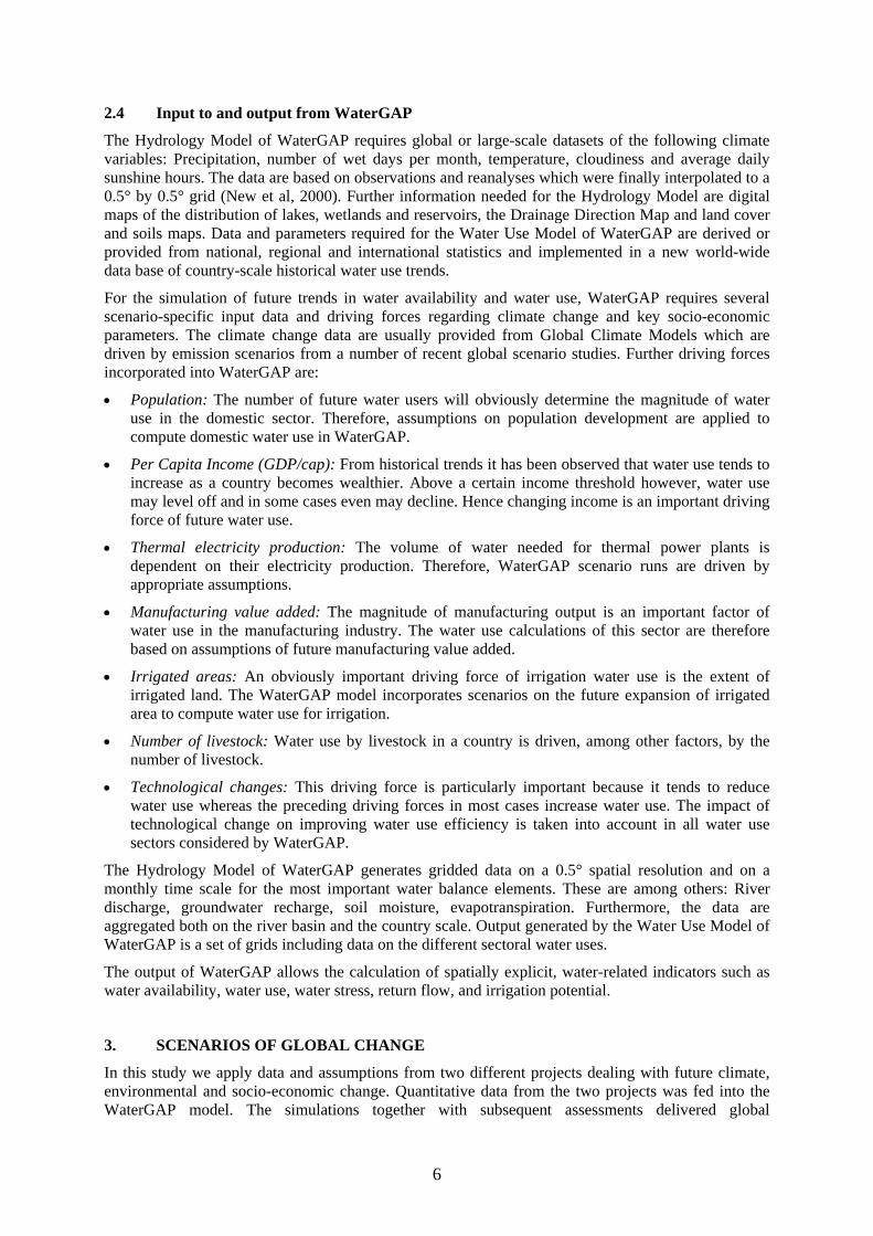
2.4 Input to and output from WaterGAP

The Hydrology Model of WaterGAP requires global or large-scale datasets of the following climate variables: Precipitation, number of wet days per month, temperature, cloudiness and average daily sunshine hours. The data are based on observations and reanalyses which were finally interpolated to a 0.5° by 0.5° grid (New et al, 2000). Further information needed for the Hydrology Model are digital maps of the distribution of lakes, wetlands and reservoirs, the Drainage Direction Map and land cover and soils maps. Data and parameters required for the Water Use Model of WaterGAP are derived or provided from national, regional and international statistics and implemented in a new world-wide data base of country-scale historical water use trends.

For the simulation of future trends in water availability and water use, WaterGAP requires several scenario-specific input data and driving forces regarding climate change and key socio-economic parameters. The climate change data are usually provided from Global Climate Models which are driven by emission scenarios from a number of recent global scenario studies. Further driving forces incorporated into WaterGAP are:

• Population: The number of future water users will obviously determine the magnitude of water use in the domestic sector. Therefore, assumptions on population development are applied to compute domestic water use in WaterGAP.

• Per Capita Income (GDP/cap): From historical trends it has been observed that water use tends to increase as a country becomes wealthier. Above a certain income threshold however, water use may level off and in some cases even may decline. Hence changing income is an important driving force of future water use.

• Thermal electricity production: The volume of water needed for thermal power plants is dependent on their electricity production. Therefore, WaterGAP scenario runs are driven by appropriate assumptions.

• Manufacturing value added: The magnitude of manufacturing output is an important factor of water use in the manufacturing industry. The water use calculations of this sector are therefore based on assumptions of future manufacturing value added.

• Irrigated areas: An obviously important driving force of irrigation water use is the extent of irrigated land. The WaterGAP model incorporates scenarios on the future expansion of irrigated area to compute water use for irrigation.

• Number of livestock: Water use by livestock in a country is driven, among other factors, by the number of livestock.

• Technological changes: This driving force is particularly important because it tends to reduce water use whereas the preceding driving forces in most cases increase water use. The impact of technological change on improving water use efficiency is taken into account in all water use sectors considered by WaterGAP.

The Hydrology Model of WaterGAP generates gridded data on a 0.5° spatial resolution and on a monthly time scale for the most important water balance elements. These are among others: River discharge, groundwater recharge, soil moisture, evapotranspiration. Furthermore, the data are aggregated both on the river basin and the country scale. Output generated by the Water Use Model of WaterGAP is a set of grids including data on the different sectoral water uses.

The output of WaterGAP allows the calculation of spatially explicit, water-related indicators such as water availability, water use, water stress, return flow, and irrigation potential.

3. SCENARIOS OF GLOBAL CHANGE

In this study we apply data and assumptions from two different projects dealing with future climate, environmental and socio-economic change. Quantitative data from the two projects was fed into the WaterGAP model. The simulations together with subsequent assessments delivered global

6

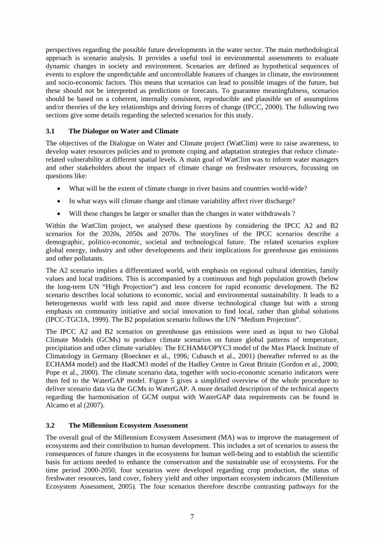
perspectives regarding the possible future developments in the water sector. The main methodological approach is scenario analysis. It provides a useful tool in environmental assessments to evaluate dynamic changes in society and environment. Scenarios are defined as hypothetical sequences of events to explore the unpredictable and uncontrollable features of changes in climate, the environment and socio-economic factors. This means that scenarios can lead to possible images of the future, but these should not be interpreted as predictions or forecasts. To guarantee meaningfulness, scenarios should be based on a coherent, internally consistent, reproducible and plausible set of assumptions and/or theories of the key relationships and driving forces of change (IPCC, 2000). The following two sections give some details regarding the selected scenarios for this study.

3.1 The Dialogue on Water and Climate

The objectives of the Dialogue on Water and Climate project (WatClim) were to raise awareness, to develop water resources policies and to promote coping and adaptation strategies that reduce climate-related vulnerability at different spatial levels. A main goal of WatClim was to inform water managers and other stakeholders about the impact of climate change on freshwater resources, focussing on questions like:

• What will be the extent of climate change in river basins and countries world-wide?

• In what ways will climate change and climate variability affect river discharge?

• Will these changes be larger or smaller than the changes in water withdrawals ?

Within the WatClim project, we analysed these questions by considering the IPCC A2 and B2 scenarios for the 2020s, 2050s and 2070s. The storylines of the IPCC scenarios describe a demographic, politico-economic, societal and technological future. The related scenarios explore global energy, industry and other developments and their implications for greenhouse gas emissions and other pollutants.

The A2 scenario implies a differentiated world, with emphasis on regional cultural identities, family values and local traditions. This is accompanied by a continuous and high population growth (below the long-term UN “High Projection”) and less concern for rapid economic development. The B2 scenario describes local solutions to economic, social and environmental sustainability. It leads to a heterogeneous world with less rapid and more diverse technological change but with a strong emphasis on community initiative and social innovation to find local, rather than global solutions (IPCC-TGCIA, 1999). The B2 population scenario follows the UN “Medium Projection”.

The IPCC A2 and B2 scenarios on greenhouse gas emissions were used as input to two Global Climate Models (GCMs) to produce climate scenarios on future global patterns of temperature, precipitation and other climate variables: The ECHAM4/OPYC3 model of the Max Planck Institute of Climatology in Germany (Roeckner et al., 1996; Cubasch et al., 2001) (hereafter referred to as the ECHAM4 model) and the HadCM3 model of the Hadley Centre in Great Britain (Gordon et al., 2000; Pope et al., 2000). The climate scenario data, together with socio-economic scenario indicators were then fed to the WaterGAP model. Figure 5 gives a simplified overview of the whole procedure to deliver scenario data via the GCMs to WaterGAP. A more detailed description of the technical aspects regarding the harmonisation of GCM output with WaterGAP data requirements can be found in Alcamo et al (2007).

3.2 The Millennium Ecosystem Assessment

The overall goal of the Millennium Ecosystem Assessment (MA) was to improve the management of ecosystems and their contribution to human development. This includes a set of scenarios to assess the consequences of future changes in the ecosystems for human well-being and to establish the scientific basis for actions needed to enhance the conservation and the sustainable use of ecosystems. For the time period 2000-2050, four scenarios were developed regarding crop production, the status of freshwater resources, land cover, fishery yield and other important ecosystem indicators (Millennium Ecosystem Assessment, 2005). The four scenarios therefore describe contrasting pathways for the

7

development of human society and ecosystems. The demand for provisioning services, such as food, fibre and water strongly increases in all four scenarios. From the four scenarios we selected two quite different future assessments, the so-called Order from Strength (OS) and the Techno Garden (TG) scenarios.

Figure 5. Schematic overview of the procedure to deliver scenario data from two different projects to WaterGAP. The dashed line indicates similarities between certain assumptions in both scenarios

According to the OS scenario, future problems are solved on a national level which leads to a fragmented world concerned with security and protection. Since global and national environmental problems are approached on a regional level and global trade is heavily regulated, economies and environmental health develop very heterogeneously across the globe. In general, economic growth rates are low (particularly in developing countries) and decrease with time. In contrast, population development is high and is projected to continuously increase beyond the year 2100. The OS scenario has some similarities with the pessimistic A2 scenario of IPCC although there are several contrasting details between both scenarios.

TG is a globalized scenario with emphasis on the introduction of new technologies and on highly managed and often engineered ecosystems. Therefore, the growth of new markets for ecosystem services is stimulated and economic growth is high. The globalization of the economies lifts many of the world’s poor into a global middle class. Population development is in the mid-range of the scenarios. However, the advantages of a globalized world are shadowed by new socio-ecological problems which come from an over-reliance of highly engineered systems. Regarding a comparison with the IPCC scenarios, TG can best be compared with the B-type, environmentally oriented scenarios (B1/B2), although it is difficult to directly compare two future assessments with their specific details.

The MA scenarios are driven by their own storylines as described above for OS and TG. The range of the greenhouse gas trends for the MA scenarios coincides well with those found in the literature, in particular the IPCC scenarios. In contrast to the WatClim project however, climate scenarios were fed to WaterGAP through the IMAGE 2 global change integrated model of RIVM which computes global land cover, climate and other indicators of global change (Figure 5).

8

3.3 Overview of scenario assumptions

Tables 1, 2 and 3 list data on input assumptions for selected driving forces of water use. The data given in Tables 1 and 2 are aggregated to the global scale since the definition of individual regions (such as e.g. Western Europe) differs between the WatClim and the MA projects. More detailed numbers, including regional and country level data are available in Alcamo et al. (2007), at www.usf.uni-kassel.de/watclim/ and at www.millenniumassessment.org

Population is projected to grow to 7.5–8.7 billion in 2020 and to 8.8–11.8 billion in 2050, depending on the scenario (Table 1). The A2 scenario is assuming the highest increase, followed by B2 and Order from Strength. The expected impact of growing population on water use is outlined in section 2.4

Table 1. The projected development of world population in the WatClim A2, B2 and the MA OS and TG scenarios. Numbers are given in millions, numbers in brackets are percentage changes in view of the 1995 reference value of 5700 million. Note that the numbers given for the WatClim A2 and B2 scenarios refer to years 2025 and 2055, respectively

period / scenario A2 B2 OS TG

2020 8722 (+53) 8032 (+41) 7777 (+36) 7537 (+32)

2050 11794 (+107) 9556 (+68) 9567 (+68) 8821 (+55)

The projected development of mean annual per capita income (expressed here as the Gross Domestic Product GDP) is projected to increase two- to fourfold in 2050, depending on the scenario (Table 2). The B2 scenario assumes the highest increase of this indicator. This is especially true for the period around the year 2050. It can be expected that increasing income leads to increasing per capita water use in most parts of the world except in the highly developed, industrialized countries.

Table 2. The projected development of annual Gross Domestic Product (GDP) per capita in the WatClim A2, B2 and the MA OS and TG scenarios. Numbers are given in percentage changes with regard to the 1995 reference value of 5102 US-Dollars. Note that the numbers given for the WatClim A2 and B2 scenarios refer to years 2025 and 2055, respectively

period / scenario A2 B2 OS TG

2020 +59 +80 +41 +60

2050 +119 +297 +93 +232

Finally, Table 3 shows the assumed rates of technological change for the computation of water use in the WatClim scenarios. Similar numbers were chosen for the MA scenarios: For OS, a low rate of improvement for technological efficiency is projected which implies a slowing of the current improvement rates. For TG, a medium to high improvement rate is assumed.

Table 3. Rate of improvement in water use efficiency (in % per year) for the three water use sectors considered in WaterGAP. Data refer to the A2 and B2 scenarios (from Alcamo et al., 2007)

period / sector domestic industry agriculture

1995-2005 2 2 0.3

2005-2025 1 1 0.3

2025-2075 1 1 0.15

9

Finally, a short summary regarding climate scenarios is given. Projected temperature increase until the mid of this century ranges around 1.5 – 2.0°C above preindustrial, with relatively slight differences between the individual scenarios. However, projected global average surface warming for the end of the 21st century is clearly scenario-dependent. Global warming is estimated to be highest under the A2- and OS-scenarios, with projected temperatures by the end of the 21st century of around 4.0°C above preindustrial. The respective numbers for B2 and TG are in the range of ca. 2.0 – 3.0°C.

The analysis of individual scenarios shows that climate change could lead to increased precipitation over more than half of the earth’s surface, with clear differences however between the scenarios and the GCM outputs. The remaining parts of the globe, including highly populated semi-arid and arid regions such as the Middle East and Southern Europe, will probably see a substantial decrease of average precipitation.

4. RESULTS

4.1 Global overview

Theoretically, increasing precipitation over larger parts of the world (as projected by the analysed scenarios; see section 3.3) will make more water available to society and ecosystems. However, the expected increase in air temperature intensifies evapotranspiration nearly everywhere, and hence reduces water availability. These two effects interact differently at different locations and produce the net increase or decrease in water availability shown in Figure 6 for the A2 scenario. Since evapotranspiration increases nearly everywhere, it tends to counteract the effect of increasing precipitation wherever it occurs. Hence the area of increasing water availability is somewhat smaller than the area of increasing precipitation.

Figure 6. Change in average annual water availability (in %) between the climate normal period (1961-1990) and the 2050s under the A2 scenario, based on climate change input from the ECHAM4 model and simulations with WaterGAP. Note that a strong projected increase in water availability (dark green colour) occurs in today’s dry parts of Northern Africa and the Near East. Therefore, an increase of 50% or more still represents comparatively low values of water availability

10

For example, under scenario A2 in the 2050s, 57 percent of the earth’s land area has increasing annual precipitation (relative to the climate normal period) as compared to 51 percent having increasing annual water availability (Alcamo et al, 2007). The two compensating effects of increasing precipitation and evapotranspiration will lead to relatively small changes in water availability up to 2050. According to the MA scenarios, global water availability is projected to increase by 5–7% only (depending on the scenario) (Millennium Ecosystem Assessment, 2005).

Increased precipitation and water availability may also be accompanied by a higher risk of flooding in many areas, especially in the humid regions. A respective investigation is presented in Alcamo et al. (2007). Similarly, an increase in water availability in one season may not be beneficial during that eventually already wet season and the surplus water is in most cases not transferable to another season.

Decreasing precipitation as projected for another major portion of the globe will (together with increasing evapotranspiration) decrease water availability in those regions. The example presented in Figure 6 demonstrates that those regions are mostly identical with today’s already water short or water scarce regions in the semi-arid and arid parts of the world, for example the northeast of Brazil, parts of Northern America, Southern Africa, Southern Europe, parts of Central Asia and Australia.

Water availability can be considered as the theoretical maximum amount of water which is exploitable by humans whereas water withdrawals give an estimated amount of water which is really abstracted to satisfy the needs of the different water use sectors. Based on the WaterGAP model, the current average global water availability is estimated to be ca. 40,000 km³ while mean annual global withdrawals amount to ca. 3600 km³, i.e., approximately 9% of estimated water availability (Figure 7). The average numbers do not indicate however that in many regions of the world the intensity of water withdrawals is high relative to water availability. How will these numbers develop according to the scenarios? Compared with water availability, water withdrawals show large changes within the next 50 years as Figure 8 demonstrates.

Figure 7. Total annual water withdrawals (in km³) and withdrawals from individual water use sectors as computed by WaterGAP for current conditions. Data are given for the entire globe (including all continents) as well as for Europe and Africa

Regarding the numbers given in Figure 8, we can follow that projected water withdrawals will substantially rise between 22% (TG) and 83% (OS) until the 2050s. Although the Order from Strength (OS) scenario does not show the largest economic growth, it shows the largest water withdrawals because of slower improvement of the efficiency of water use and a strong population growth. In Techno Garden (TG), fast improvements in water use efficiency result in the lowest growth rate of water withdrawals.

11

Figure 8. Projected average annual water withdrawals (in km³) in the investigated scenarios for the period around year 2050. The WatClim scenarios refer to ECHAM4 climate change input to WaterGAP

A more detailed, regional picture of projected water withdrawals delivers Figure 9. It presents results from the B2 scenario which serves as a good example for differences in regional projections. The graph demonstrates that water withdrawals are expected to increase substantially in sub-Saharan Africa, Latin America, major parts of Asia and some other developing regions while they remain at the current level or decrease in most industrial countries. The projected effect of increasing population and economic growth in today’s less developed countries leads to a strong increase in the domestic and industrial water use sectors which clearly over-compensate the assumed improvements in water use efficiency. According to the scenarios, many more people gain access to a water supply in those regions, as domestic water use is projected to substantially increase. The slight changes in projected water withdrawals in the developed world can be attributed to different factors, such as a continuation in the efficiency of water use and a decline in domestic water use because nearly the entire population has already today access to an adequate water supply.

Figure 9. Projected changes in water withdrawals (in %) under the B2 scenario for the period around 2050, based on climate change input from the ECHAM4 model and simulations with WaterGAP

12

The projected changes in water availability and water withdrawals will have consequences on future water stress. We define here water stress as an indicator for the intensity of pressure put on water resources and aquatic ecosystems by external drivers of change (Alcamo et al., 2007). The higher the amount of water withdrawn for human use the higher the water stress since part of the withdrawn water equals consumptive use (i.e., it evaporates to the atmosphere) while another part of the used water is discharged back into a lake or river, but with higher degrees of pollution. But water stress also includes the pressure on water resources caused by climate change since climate change can lead to reduced average water availability. We assume therefore that high levels of water stress lead to high limitations to freshwater ecosystems and consequently chronic or acute shortages of water supply may occur.

A common indicator of water stress is the annual “withdrawals-to-availability ratio” (w.t.a.) which divides total withdrawals by total annual water availability. The advantage of the w.t.a indicator is that it incorporates the long term effects of changing water use on water stress. Following international convention, severe water stress occurs when the approximate threshold of w.t.a is greater than 0.4. River basins exceeding this threshold are presumed to have a higher risk of chronic water shortages. There are at least two other water stress indicators discussed and applied in the international literature. Alcamo et al. (2007) explicitly discuss the different approaches and present results for water stress computed with three different indicators.

Today, about 22% of the world’s river basin area falls into the category of severe water stress with about 2.3 billion people who live in these regions. It is clear that future water stress will tend to increase in those regions where water withdrawals are projected to increase (i.e., through socio-economic development) and/or water availability will decrease (i.e., through climate change), while water stress will decrease because of decreasing withdrawals and/or growing water availability. The projected development of water stress is shown in Figure 10 for the A2 scenario. According to this scenario, the regions in the severe water stress category in the 2050s include much of northern and southern Africa, the Middle East, Central Asia, southern Asia, northern China, the western United States, and the west coast and northeast of Latin America.

Figure 10. Water stress expressed by the w.t.a ratio in the 2050s for the A2 scenario (climate change input from the ECHAM4 model and simulations with WaterGAP)

13

The trends towards increasing land areas with severe water stress are similar for the WatClim and the MA scenarios. In comparison with today’s conditions, they expand especially in those regions of the world where strong increases in water withdrawals are expected. Under the OS scenario, water withdrawals increase sharply as described above (Figure 8) while under TG withdrawals grow more slowly in most parts of the world. Therefore, the spatial extent of area under severe water stress (Figure 11) and the number of people living in water stressed regions differ between the scenarios, but the general, projected development is similar. According to our calculations and the different scenarios, the number of people living in regions with severe water stress is projected to increase from 2.3 billion today (1995) to 3.8 – 4.1 in the 2020s and to 5.2 – 6.8 billion in the 2050s.

Figure 11. The development of the spatial extent of area under severe water stress (w.t.a > 0.4) according to the WatClim scenarios. The range of the estimates which stems from two emission scenarios and two different GCMs is indicated

It is obvious that according to the different scenarios, some areas, especially in the highly industrialized countries, fall out of the severe water stress category. The reasons for this development are: stabilizing withdrawals (Figure 9) and increasing water availability (Figure 6) due to higher precipitation under climate change.

As pointed out before, the area of water stress changes with time as socio-economic drivers produce different patterns of water withdrawals and climate change different patterns of water availability. The question is now which of the two drivers have a higher degree of impact regarding changes in water stress. With respect to Figure 6 (changing, mainly increasing water availability due to climate change) and Figures 8 and 9 (changing water withdrawals mainly due to socio-economic development) we can state that the principal cause of increasing water stress is growing water withdrawals as a consequence of growing population and improving economical conditions. Alcamo et al (2007) give the following numbers with regard to the WatClim scenarios and the scenario period of the 2050s:

Global land area with increasing water stress = 61 – 75% • thereof areal share of increasing water withdrawals: 87 – 90% • thereof areal share of decreasing water availability: 10 – 13%

In the regions where a decrease of water stress is projected, climate change plays a major role through increasing water availability, followed by assumed reductions in water withdrawals for the reasons described above. Alcamo et al (2007) report the following numbers (again for WatClim calculations and the years around 2050:

Global land area with decreasing water stress = 14 – 29% • thereof areal share of decreasing water withdrawals: 17 – 47% • thereof areal share of increasing water availability: 53 – 83%

To summarize, water stress significantly changes over most river basins although the intensity of change and its direction is very geographically- and scenario-dependent. Both changing water availability and withdrawals are important factors in determining the direction of change. Under the

14

scenarios analyzed, increasing water stress is caused mainly (on an areal basis) by increasing water withdrawals (dominance of socio-economic factors), whereas decreasing water stress is caused mainly by increasing water availability related to increasing precipitation (dominance of climate factors).

4.2 Regional results

A regional view of changing conditions in the water sector is carried out to demonstrate differences between the regions and the scenarios and to underline existing uncertainties. Regarding the two scenario exercises it is difficult however to carry out comparisons on the regional level. This is due to differences in the definition of individual regions. For example, the WatClim project identifies the African continent as one region, while in MA two regions exist which cover parts of Africa: the MA regions “Middle East and North Africa” and “Sub-Saharan Africa”.

The comparison of water withdrawals between Europe and Africa (Figure 12) demonstrates the projected, rapid increase of water use on the African continent, with relatively small differences between the WatClim A2 and B2 scenarios (except for the 2070s). Further uncertainties of these ECHAM4-based estimates may arise when the climate change information from HadCM3 is included (not analysed here). According to the MA scenarios for the MA region “Sub Saharan Africa”, water withdrawals are projected to double compared to the current numbers, i.e., from 100 km³ today to 200 km³ in 2050 for both OS and TG.

Figure 12. Current (year 1995) and projected water withdrawals (in km³) in Europe and Africa based on the WatClim scenarios (ECHAM4 climate change input to WaterGAP)

The projections presented in Figure 12 for future water withdrawals in Europe show that only slight increases may occur, with small differences between A2 and B2. No respective numbers are available for the MA scenarios since Europe belongs to the “OECD countries”-group and no disaggregation of the data was possible. It should be pointed out that the conditions within Europe regarding current and future water availability and water withdrawals are very different, and it is advisable to make a separation between Northern and Southern Europe. Projections for Northern Europe show decreasing levels of water withdrawals within the next 50 years, with a simultaneous increase in water availability. In contrast, Southern Europe will face higher water stress levels than today since water withdrawals are projected to increase (mainly because of higher irrigation water demands due to climate change), while water availability will decrease (for further details see http://scenarios.ewindows.eu.org/reports/fol949029).

Since natural conditions as well as socio-economic drivers differ widely across the globe, we included selected case studies for a detailed assessment of water related issues. The selection was mainly based on the catchments investigated within the EU-funded NeWater project (www.newater.info) and includes the Tisza, Rhine, Guadiana (all in Europe) and Orange (Southern Africa) catchments. In the following paragraphs, some findings for the Guadiana and Orange basins are reported. At the end of

15

this section, we also present some findings from a project dealing with water resources development in the Jordan River Region. It is important to note that we do not consider possible mitigation measures regarding the reduction of water stress in our simulations – both on the global and the regional scale –, with the clear exception of increasing water use efficiencies (see Table 3). Therefore, already existing or planned regional measures, such as interbasin transfers of water or the construction and operation of reservoirs for drinking water supply are not considered in WaterGAP.

The Guadiana river drains a catchment area of approximately 67,500 km² and is located in the centre of Spain and parts of Portugal. Today, only around 1.7 million people live in this water scarce region where irrigated agriculture is the highest water consumer. According to our simulations, the Guadiana and its broader environs are already today in the severe water stress category of the w.t.a indicator. Population projections are very contradictory in the different scenarios. For the scenario period of the 2050s, a drastic population decrease is projected in the OS (1.2 million), the TG (1.4 million) and the B2 (1.5 million) scenarios, while the A2 scenario assumes a slight population increase (1.8 million). These differing numbers and the different scenario assumptions induce a very heterogeneous picture of the future water conditions in the Guadiana. Figure 13 shows the projected development (for the 2050s) of both water availability and water withdrawals for all investigated scenarios.

Figure 13. Current conditions (1995) and future projections (2050s) of mean annual water availability and mean annual water withdrawals (in km³) in the Guadiana river basin

First of all, the high amount of current withdrawals compared to the naturally available water is obvious (note that the numbers given in Figure 13 – including those for the current state – come from WaterGAP simulations). The future development regarding water availability in the Guadiana is very unclear as particularly the WatClim scenarios show very different developments. This is not only due to differences between the WatClim A2 and B2 scenarios, but also due to obvious differences between the outputs of the two GCMs. Therefore, the possible range of future water availability includes both a drastic reduction (ECHAM4 – A2 GCM/scenario combination) and a medium size increase (HadCM3 – B2). The two MA scenarios lead to simulated, slight decreases in water availability.

Surprisingly, the projected water withdrawals are very similar between the scenarios (Figure 13). An exception is the MA-OS scenario which leads to a strong increase in the future water withdrawals although the same scenario assumes the highest reduction in future population in the Guadiana (see above). The principal cause for this development seems to be a projected increase in irrigated land. The combination with a warmer and drier future climate therefore leads to a strong rise in future irrigation water demand. The other investigated scenarios lead to slight decreases in future projections of water demand. It is clear that even though the projections for future water availability and water demand show a high range of possible developments, future water stress conditions in the Guadiana basin will remain on a severe level.

Our second example of regional scenario analysis deals with the occurrence of water stress in the Orange basin in Southern Africa. The Orange (also called Oranje) is a large river basin, with a

16

catchment area of approximately 896,000 km². Its watershed covers major parts of South Africa, Lesotho, Botswana and Namibia. The climate conditions are mostly dry and warm semi-arid. Currently, approximately 14 million people live in the Orange catchment, a part of them in notable urban centres of which Bloemfontein (approx. 500,000 inhabitants) is the largest. In Southern Africa, the Orange ranks among the rivers which have experienced the highest degrees of human impacts, such as the building of dams, reservoirs and power plants and the establishment of a number of interbasin transfers in order to satisfy the high water demands of the region. Today, agriculture is the highest water consumer (ca. 64% of total water withdrawals), followed by the domestic sector (ca. 29%).

Population projections for the Orange show two contrasting developments. According to the WatClim project, population numbers are projected to drastically increase from 14 millions today to around 30 million people in the 2050s, i.e., a doubling of the current numbers is assumed. Differences between A2 and B2 are very small. The MA scenarios however assume slight decreases in the number of people, from currently 14 million to 12.5 million (OS) and 10.5 million (TG), respectively.

Water availability is projected to decrease in all scenarios (Figure 14) due to climate change, with a surprisingly small range of scenario results. Future conditions regarding water withdrawals show increasing trends (with the exception of the TG scenario). This is mainly due to rising water demands in the domestic sector, even under the population decrease scenario OS (in which an intensification of irrigated agriculture, accompanied by only small improvements in water use efficiency, is assumed). According to the TG scenario however, a clear decrease of future water withdrawals arises. This is a consequence of the projected population decrease and the fast introduction of water saving innovations in the water use sectors.

Figure 14. Current conditions (1995) and future projections (2050s) of mean water availability and mean water withdrawals (in km³) in the Orange river basin. Note that the scales of the two graphs are different

The current extent and future development of water stress in the Southern African region is shown on the maps of Figure 15. According to our simulations, severe water stress occurs already today in the Orange and some of its neighbouring catchments. On the other hand, it is apparent that there are a number of basins in the low water stress category. This can be explained by relatively low population densities and related low water withdrawals (very probably this applies to most of the low water stressed basins of the region) or higher water availabilities (this might be the case at the eastern coast of Southern Africa). The results of two selected scenarios (WatClim-A2, with climate change information from two GCMs, and MA-TG) show that the possible future stretch of severe water stress agrees to a certain extent between the individual scenarios / model runs for the period of the 2050s. The projected increase of severe water stress in Southern Africa mainly includes parts of the region along the dry western coast of South Africa and Namibia, but the total area newly assigned to the severe stress category is comparatively small. This might be caused by similar reasons as mentioned above: a general decrease of water availability in the region (as a consequence of climate change) contrasts with relatively low population densities and low agricultural activities. On the other side will

17

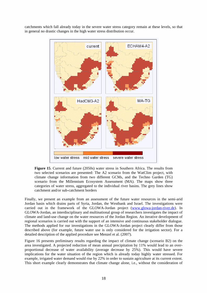
catchments which fall already today in the severe water stress category remain at these levels, so that in general no drastic changes in the high water stress distribution occur.

Figure 15. Current and future (2050s) water stress in Southern Africa. The results from two selected scenarios are presented: The A2 scenario from the WatClim project, with climate change information from two different GCMs, and the Techno Garden (TG) scenario from the Millennium Ecosystem Assessment (MA). The maps show three categories of water stress, aggregated to the individual river basins. The grey lines show catchment and/or sub-catchment borders

Finally, we present an example from an assessment of the future water resources in the semi-arid Jordan basin which drains parts of Syria, Jordan, the Westbank and Israel. The investigations were carried out in the framework of the GLOWA-Jordan project (www.glowa-jordan-river.de). In GLOWA-Jordan, an interdisciplinary and multinational group of researchers investigates the impact of climate and land-use change on the water resources of the Jordan Region. An iterative development of regional scenarios is carried out with the support of an intensive and continuous stakeholder dialogue. The methods applied for our investigations in the GLOWA-Jordan project clearly differ from those described above (for example, future water use is only considered for the irrigation sector). For a detailed description of the applied procedure see Menzel et al. (2007).

Figure 16 presents preliminary results regarding the impact of climate change (scenario B2) on the area investigated. A projected reduction of mean annual precipitation by 11% would lead to an over-proportional decrease of water availability (average decrease by 25%). This would have severe implications for the water situation of the region which is already today highly water stressed. For example, irrigated water demand would rise by 22% in order to sustain agriculture at its current extent. This short example clearly demonstrates that climate change alone, i.e., without the consideration of

18

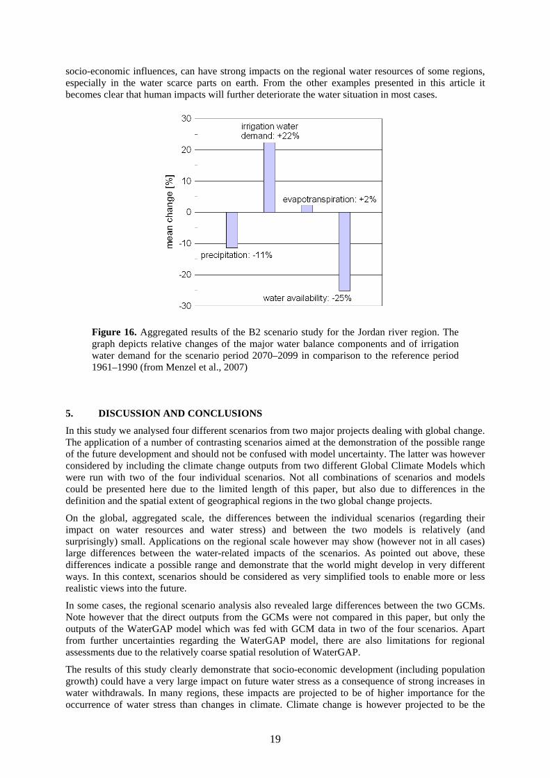
socio-economic influences, can have strong impacts on the regional water resources of some regions, especially in the water scarce parts on earth. From the other examples presented in this article it becomes clear that human impacts will further deteriorate the water situation in most cases.

Figure 16. Aggregated results of the B2 scenario study for the Jordan river region. The graph depicts relative changes of the major water balance components and of irrigation water demand for the scenario period 2070–2099 in comparison to the reference period 1961–1990 (from Menzel et al., 2007)

5. DISCUSSION AND CONCLUSIONS

In this study we analysed four different scenarios from two major projects dealing with global change. The application of a number of contrasting scenarios aimed at the demonstration of the possible range of the future development and should not be confused with model uncertainty. The latter was however considered by including the climate change outputs from two different Global Climate Models which were run with two of the four individual scenarios. Not all combinations of scenarios and models could be presented here due to the limited length of this paper, but also due to differences in the definition and the spatial extent of geographical regions in the two global change projects.

On the global, aggregated scale, the differences between the individual scenarios (regarding their impact on water resources and water stress) and between the two models is relatively (and surprisingly) small. Applications on the regional scale however may show (however not in all cases) large differences between the water-related impacts of the scenarios. As pointed out above, these differences indicate a possible range and demonstrate that the world might develop in very different ways. In this context, scenarios should be considered as very simplified tools to enable more or less realistic views into the future.

In some cases, the regional scenario analysis also revealed large differences between the two GCMs. Note however that the direct outputs from the GCMs were not compared in this paper, but only the outputs of the WaterGAP model which was fed with GCM data in two of the four scenarios. Apart from further uncertainties regarding the WaterGAP model, there are also limitations for regional assessments due to the relatively coarse spatial resolution of WaterGAP.

The results of this study clearly demonstrate that socio-economic development (including population growth) could have a very large impact on future water stress as a consequence of strong increases in water withdrawals. In many regions, these impacts are projected to be of higher importance for the occurrence of water stress than changes in climate. Climate change is however projected to be the

19

major cause for decreasing water stress, but the spatial extent of the regions with future decreases in water stress is very limited. These results could lead to the assumption that climate change is seen as a less important component regarding the occurrence of future water problems (an exception is the example from the Jordan region presented in section 4.2). It has to be pointed out however that we did not investigate the impact of climate change on the seasonal development of water stress neither we analysed the future occurrence of hydrological extremes. From the results of a large number of climate impact studies follows that the possible impact of climate change on the hydrological cycle, the distribution of water resources and future water demand will probably be stronger and more severe than discussed in the context of this study. Finally, it has to be emphasized that some factors (such as global population growth) could decline in importance during a certain period while others (such as climate change) could gain more importance. This is especially true for the second half of the 21st century, when climate change probably accelerates.

ACKNOWLEDGEMENTS

A part of this study was supported by the EU-funded NeWater project (“New approaches to adaptive water management under uncertainty”), contract number 511179. We are grateful to Sabrina Kümmritz for her support with the regional scenario analysis.

REFERENCES

Alcamo, J., Flörke, M., Märker, M. (2007). Future long-term changes in global water resources driven by socio-economic and climate changes. Hydrol. Sci. J. 52, 247-275.

Alcamo, J., Döll, P., Henrichs, T., Kaspar, F., Lehner, B. Rösch, T., Siebert, S. (2003a). Development and testing of the WaterGAP2 global model of water use and availability. Hydrol. Sci. J. 48, 317-337.

Alcamo, J., Döll, P., Henrichs, T., Kaspar, F., Lehner, B. Rösch, T., Siebert, S. (2003b). Global estimation of water withdrawals and availability under current and “business as usual“ conditions. Hydrol. Sci. J. 48, 339-348.

Alcamo, J., Henrichs, T., Rösch, T. (2000). World Water in 2025 – Global Modeling Scenarios for the World Commission on Water for the 21st Century. World Water Series Report 2, Center for Environmental Systems Research, University of Kassel, Germany.

Cubasch, U., Meehl, G.A., Boer, G.J., Stouffer, R.J., Dix, M., Noda, A., Senior, C.A., Raper, S., Yap, K.S. (2001). Projections of future climate change. In: Climate Change 2001: The Scientific Basis. Contribution of Working Group I to the Third Assessment Report of the Intergovernmental Panel on Climate Change (IPCC). Cambridge University Press, Cambridge, UK.

Döll, P., Kaspar, F., Lehner, B. (2003). A global hydrological model for deriving water availability indicators: model tuning and validation. J. Hydrol. 270, 105-134.

Döll, P., Lehner, B. (2002). Validation of a new global 30-min drainage direction map. J. Hydrol. 258, 214-231.

Döll. P., Siebert, S. (2002). Global modelling of irrigation water requirements. Water Resour. Res. 38, 8.1-8.10.

Gordon, C., Cooper, C., Senior, C.A., Banks, H., Gregory, J.M., Johns, T.C., Mitchell, J.F.B., Wood, R.A. (2000). The simulation of SST, sea ice extents and ocean heat transports in a version of the Hadley Centre coupled model without flux adjustments. Clim. Dyn. 16, 147-168.

IPCC (Intergovernmental Panel on Climate Change) (2000). Special Report on Emission Scenarios. Report of the Working Group III of the IPCC (ed. by Nakicenovic, N., Swart, R.). Cambridge University Press, Cambridge, UK.

20

21

IPCC-TGCIA (1999). Guidelines on the Use of Scenario Data for Climate Impact and Adaptation Assessment. Version 1. Prepared by Carter, T.R., Hulme, M. and Lal, M. Intergovernmental Panel on Climate Change, Task Group on Scenarios for Climate Impact Assessment, 69pp

Menzel, L., Teichert, E., Weiss, M. (2007). Climate change impact on the water resources of the semi-arid Jordan region. In: Heinonen, M. (ed.): Proc. 3rd International Conference on Climate and Water, Helsinki, 320 – 325 (available at www.usf.uni-kassel.de publications)

Millennium Ecosystem Assessment (2005). Ecosystems and Human Well-being: Synthesis. Island Press, Washington, DC.

New, M., Hulme, M., Jones, P. (2000). Representing twentieth-century space-time climate variability. Part II: Development of 1901-96 monthly grids of terrestrial surface climate. J. Climate 13, 2217-2238.

Pope, V., Gallani, M., Rowntree, P., Stratton, R. (2000). The impact of new physical parameterizations in the Hadley Centre climate model – HadCM3. Clim. Dyn. 16, 123-146.

Roeckner, E., Arpe, K., Bengtsson, L., Christoph, M., Claussen, M., Dümenil, L., Esch, M., Giorgetta, M., Schlese, U., Schulzweida, U. (1996). The atmospheric general circulation model ECHAM4: Model description and simulation of present-day climate. Report no. 218, Max Planck Institut für Meteorologie, Hamburg, Germany.

Siebert, S., Hoogeveen, J., Frenken, K. (2006). Irrigation in Africa, Europe and Latin America. Update of the Digital Global Map of Irrigation Areas to Version 4. Frankfurt Hydrology Paper 05, University of Frankfurt (Main), Germany and FAO, Rome, Italy.