impact of biodiesel fuels on air quality and human … toxics modeling model performance evaluation...

May 2003 • NREL/SR-540-33798

R.E. Morris and Y. Jia ENVIRON International Corporation Novato, California

Impact of Biodiesel Fuels on Air Quality and Human Health: Task 5 Report Air Toxics Modeling of the Effects of Biodiesel Fuel Use on Human Health in the South Coast Air Basin Region of Southern California

National Renewable Energy Laboratory 1617 Cole Boulevard Golden, Colorado 80401-3393 NREL is a U.S. Department of Energy Laboratory Operated by Midwest Research Institute • Battelle • Bechtel

Contract No. DE-AC36-99-GO10337

May 2003 • NREL/SR-540-33798

Impact of Biodiesel Fuels on Air Quality and Human Health: Task 5 Report Air Toxics Modeling of the Effects of Biodiesel Fuel Use on Human Health in the South Coast Air Basin Region of Southern California

R.E. Morris and Y. Jia ENVIRON International Corporation Novato, California

NREL Technical Monitor: K.S. Tyson and R. McCormick Prepared under Subcontract No. AXE-9-29079-01

National Renewable Energy Laboratory 1617 Cole Boulevard Golden, Colorado 80401-3393 NREL is a U.S. Department of Energy Laboratory Operated by Midwest Research Institute • Battelle • Bechtel

Contract No. DE-AC36-99-GO10337

NOTICE This report was prepared as an account of work sponsored by an agency of the United States government. Neither the United States government nor any agency thereof, nor any of their employees, makes any warranty, express or implied, or assumes any legal liability or responsibility for the accuracy, completeness, or usefulness of any information, apparatus, product, or process disclosed, or represents that its use would not infringe privately owned rights. Reference herein to any specific commercial product, process, or service by trade name, trademark, manufacturer, or otherwise does not necessarily constitute or imply its endorsement, recommendation, or favoring by the United States government or any agency thereof. The views and opinions of authors expressed herein do not necessarily state or reflect those of the United States government or any agency thereof.

Available electronically at http://www.osti.gov/bridge

Available for a processing fee to U.S. Department of Energy and its contractors, in paper, from:

U.S. Department of Energy Office of Scientific and Technical Information P.O. Box 62 Oak Ridge, TN 37831-0062 phone: 865.576.8401 fax: 865.576.5728 email: [email protected]

Available for sale to the public, in paper, from:

U.S. Department of Commerce National Technical Information Service 5285 Port Royal Road Springfield, VA 22161 phone: 800.553.6847 fax: 703.605.6900 email: [email protected] online ordering: http://www.ntis.gov/ordering.htm

Printed on paper containing at least 50% wastepaper, including 20% postconsumer waste

http://www.osti.gov/bridge

http://www.ntis.gov/ordering.htm

ES-1

EXECUTIVE SUMMARY INTRODUCTION Biodiesel fuels have been investigated for a number of reasons, such as an extender for petroleum-based fuels derived from a domestic renewable energy source. But lately the primary interest is the potential for a more environmentally benign fuel. One potential benefit of biodiesel is that it can biologically degrade, making spills and leaks less of a concern. However, the potential for exhaust emission reductions and reductions in emissions toxicity are of the most interest. Several studies have shown that large reductions in hydrocarbon, particulate, and carbon monoxide emissions are expected from its use either as a neat fuel or as a blend with petroleum-derived fuels. Objective The objective of Task 5 of the NREL Biodiesel Fuels Impacts of Air Quality and Human Health Study are to estimate the effects biodiesel fuel use in the South Coast (Los Angeles) Air Basin (SoCAB) of Southern California (SoCAB) would have on air toxics risk, exposure, and human health. CONCLUSIONS An analysis of engine test data has found that a 20%/80% biodiesel/standard diesel (B20) fuel reduces tailpipe diesel particulate matter (PM) emissions by approximately 9 percent and reduces the toxicity of the diesel PM by approximately 5 percent (Lindhjem and Pollack, 2000). These effects were accounted for in air toxics modeling the South Coast Air Basin (SoCAB) region of Southern California for three emission scenarios:

• Standard diesel emissions based on the EMFAC2000 mobile source emissions model; • 100% penetration of a B20 biodiesel fuel in the Heavy Duty Diesel Vehicle (HDDV)

fleet; and • 50% penetration of a B20 biodiesel fuel in the HDDV fleet.

The air toxics modeling accounted for diesel PM, four organic air toxics (benzene, 1, 3-butadiene, formaldehyde, and acetaldehyde) and hexavalent chromium that, according to the South Coast Air Quality Management District (SCAQMD) Multiple Air Toxics and Exposure Study (MATES-II), accounts for over 90 percent of the risk associated with exposure to air toxic compounds in the SoCAB. The conclusions of the biodiesel impacts on exposure and human health study are as follows:

• The use of a B20 fuel in the HDDV fleet is estimated to reduce the one in a million risk of premature death due to exposure to air toxics in the SoCAB by approximately 2 and 5 percent for the 50% and 100% HDDV fleet penetration scenarios, respectively.

ES-2

• The use of the B20 biodiesel fuel in the HDDV fleet is estimate to reduce the potential for premature death in the SoCAB due to a long-term exposure to air toxics by approximately 2 percent for the 50% penetration scenario and by approximately 5-6 percent for the 100% penetration scenario.

1

TABLE OF CONTENTS

Page EXECUTIVE SUMMARY ES-1 Introduction..........................................................................................................................ES-1 Conclusion ...........................................................................................................................ES-1 1. INTRODUCTION................................................................................................................ 1-1

Background ............................................................................................................................ 1-1 Overview of Approach........................................................................................................... 1-2

2. DEVELOPMENT OF MODEL INPUTS.......................................................................... 2-1

Modeling Domain .................................................................................................................. 2-1 Meteorological Inputs ............................................................................................................ 2-1 Air Quality Data..................................................................................................................... 2-2 Initial and Boundary Conditions............................................................................................ 2-3 Emissions .............................................................................................................................. 2-6

3. AIR TOXICS MODELING MODEL PERFORMANCE EVALUATION USING THE MATES-II DATABASE................................................... 3-1

Model Performance Evaluation ............................................................................................. 3-2 Spatial Distribution of Air Toxic Concentrations................................................................ 3-16 Summary of Model Performance......................................................................................... 3-19

4. EFFECTS OF BIODIESEL FUELS ON RISK AND EXPOSURE.................................. 4-1

Risk Calculation and Exposure Modeling ............................................................................. 4-2

REFERENCES.......................................................................................................................... R-1

APPENDICES

Appendix A: Spatial Distribution of Annual Average Concentrations Estimated by CAMx/EMFAC2000

2

TABLES

Table 2-1. Initial and boundary conditions used for the CAMx/RTRAC air toxics modeling .................................................................... 2-3 Table 2-2. Emissions adjustment factors used to update the MATES-II EMFAC7G on-road mobile source emissions to EMFAC2000 levels. ............... 2-7 Table 2-3. Summary of annual air toxics emission totals (lb/day) for the South Coast Air Basin (SoCAB) from MATES-II using EMFAC7G and updated using EMFAC2000. ........................................... 2-8 Table 3-1. Summary model performance evaluation statistics for benzene (predicted minus observed, positive bias implies overprediction). ....................................................................................... 3-3 Table 3-2. Summary model performance evaluation statistics for 1,3-butadiene (predicted minus observed, positive bias implies overprediction)................................................................................. 3-4 Table 3-3. Summary model performance evaluation statistics for acetaldehyde (predicted minus observed, positive bias implies overprediction)................................................................................. 3-6 Table 3-4. Summary model performance evaluation statistics for formaldehyde (predicted minus observed, positive bias implies overprediction)................................................................................. 3-8 Table 3-5. Summary model performance evaluation statistics for chromium PM2.5 (predicted minus observed, positive bias implies overprediction)............................................................................... 3-10 Table 3-6. Summary model performance evaluation statistics for Hexavalent Chromium PM2.5 (predicted minus observed, positive bias implies overprediction)................................................. 3-12 Table 3-7. Summary model performance evaluation statistics for Elemental Carbon PM2.5 (predicted minus observed, positive bias implies overprediction)................................................. 3-14 Table 4-1. Diesel particulate matter emissions in SoCAB modeling domain for the three

emission scenarios (lb/day).................................................................................. 4-1 Table 4-2. Average risk (out of a million) of premature death due to exposure to air toxics in the SoCAB for the standard diesel scenario calculated with no indoor/outdoor (I/O) effects and accounting for indoor/outdoor effects on an annual average and hourly basis............................ 4-3 Table 4-3. Average risk (out of a million) of premature death due to exposure to air toxics for the standard diesel, 50% penetration of B20 in the HDDV fleet, and 100% penetration of B20 in the SoCAB in the HDDV fleet scenarios calculated with no indoor/outdoor (I/O) effects and accounting for indoor/outdoor effects on an annual average and hourly basis............................ 4-3

3

Table 4-4. SoCAB-wide exposure in terms of number of premature death due to exposure to air toxics for the standard diesel, 50% penetration of B20 in the HDDV fleet, and 100% penetration in the HDDV fleet scenarios calculated with no indoor/outdoor (I/O) effects and accounting for indoor/outdoor effects on an annual average and hourly..................................... 4-4

FIGURES

Figure ES-1. Annual average fine (PM2.5) (top) and coarse (PM2.5-10) (bottom) diesel particulate mater concentrations (µg/m3) in the SoCAB estimated by the CAMx/EMFAC2000.......................................ES-6 Figure 2-1. Location of surface meteorological (red x), upper-air meteorological (blue diamonds), and precipitation (green boxes) sites in the SoCAB used for the April 1998 – March 1999 CALMET modeling. .................................................. 2-4 Figure 2-2. Location of the 10 MATES-II fixed sites air toxics samplers. ............................................................................. 2-5 Figure 3-1. Scatter plot of predicted and observed 24-hour benzene concentrations (µg/m3)........................................................................... 3-3 Figure 3-2. Scatter plot of predicted and observed 24-hour 1,3-butadiene concentrations (µg/m3) ................................................................. 3-5 Figure 3-3. Scatter plot of predicted and observed 24-hour acetaldehyde concentrations (µg/m3). .................................................................. 3-7 Figure 3-4. Scatter plot of predicted and observed 24-hour formaldehyde concentrations (µg/m3).................................................................. 3-9 Figure 3-5. Scatter plot of predicted and observed 24-hour chromium concentrations (µg/m3) ..................................................................... 3-11 Figure 3-6. Scatter plot of predicted and observed 24-hour hexavalent chromium concentrations (µg/m3) ................................................... 3-13 Figure 3-7. Scatter plot of predicted and observed 24-hour elemental carbon concentrations (µg/m3) .......................................................... 3-15 Figure 4-1a. Spatial distribution of estimated risk (out of a million) for the standard diesel scenario not accounting for indoor/outdoor effects. ......................................................................................... 4-5 Figure 4-1b. Spatial distribution of estimated risk (out of a million) for the standard diesel scenario accounting for indoor/outdoor effects on an annual basis. .......................................................... 4-6 Figure 4-1c. Spatial distribution of estimated risk (out of a million) for the standard diesel scenario accounting for indoor/outdoor effects on an hourly basis............................................................ 4-7

1-1

1. INTRODUCTION BACKGROUND Biodiesel fuels have been investigated for a number of reasons, such as an extender for petroleum-based fuels derived from a domestic renewable energy source. But lately the primary interest is the potential for a more environmentally benign fuel. One potential benefit of biodiesel is that it can biologically degrade, making spills and leaks less of a concern. However, the potential for exhaust emission reductions and reductions in emissions toxicity are of the most interest. Several studies have shown that large reductions in hydrocarbon, particulate, and carbon monoxide emissions are expected from its use either as a neat fuel or as a blend with petroleum-derived fuels. There have been several studies regarding the effects of biodiesel fuels on exhaust emissions of NOx, VOC, CO, and particulate matter (PM). Almost all of these studies have examined emissions from heavy-duty diesel vehicle (HDDV) engines. However, the effects of biodiesel use on ambient air quality have not been quantified. Thus, the National Renewable Energy Laboratory (NREL) has retained ENVIRON International Corporation to estimate the air quality and resultant and health effect toxic impacts from the use of biodiesel fuels in several cities in the U.S. Effects of Biodiesel Fuel on Risk, Exposure, and Human Health Diesel Particulate Matter (PM) has been declared a toxic compound by the state of California. Analyses of diesel PM reveals that it contains toxic compounds that fall into a general category know as polyaromatic hydrocarbons (PAHs) and nitro-PAHs. These compounds have been identified as causing cancer in humans when exposed to high concentrations over long time periods. Under Task 1 of the NREL biodiesel impacts study, diesel and biodiesel engine emissions test data were analyzed for emissions effects and the presence of PAHs and nitro-PAHs and it was found that not only did biodiesel fuels emit less diesel PM than standard diesel, but there were also less PAHs and nitro-PAHs in the biodiesel PM emissions (Lindhjem and Pollack, 2000). Thus, use of biodiesel would not only reduce diesel PM emissions but also diesel PM toxicity so would result in lower air toxics risk and exposure than use of a standard diesel fuel. During April 1998 to March 1999, the South Coast Air Quality Management District (SCAQMD) conducted the second Multiple Air Toxics and Exposure Study (MATES-II) in the South Coast (Los Angeles) Air Basin (SoCAB) that consisted of air quality monitoring and modeling of air toxics and risk and exposure calculations. MATES-II concluded that 70% of the risk of premature death due to exposure to air toxics in the SoCAB was due exposure to diesel PM. Thus, the use of biodiesel fuel could have a beneficial effect on air toxics risk and exposure.

1-2

Purpose This document is the Task 5 Report for the NREL “Impacts of Biodiesel Fuels on Air Quality and Human Health “ study. The objective of Task 5 is to estimate the effects of the use of biodiesel fuels on air toxics and resultant risk, exposure, and human health. Annual air toxics modeling of the South Coast (Los Angeles) Air Basin (SoCAB) region of Southern California was conducted for a standard diesel and two biodiesel fuel scenarios and the effects on risk and exposure were calculated. OVERVIEW OF APPROACH As part of the Multiple Air Toxics Exposure Study (MATES-II), the South Coast Air Quality Management District (SCAQMD) applied the UAM-Tox photochemical and air toxics grid model for a year (April 1998-March 1999). Air toxic concentration estimates were obtained across the South Coast (Los Angeles) Air Basin (SoCAB) for approximately 50 toxic compounds. The UAM-Tox used a 105 by 60 horizontal array of 2-km by 2-km grid cells to cover the SoCAB and five vertical layers up to a region top of 2-km above ground level (AGL). Hourly three-dimensional meteorological inputs were generated for April 1, 1998 through March 31, 1999 using the CALMET diagnostic meteorological model and surface and upper-air meteorological observations. The UAM-Tox emissions inventory inputs were generated by the SCAQMD for the expanded CB-IV chemical mechanism (TOX mechanism) that explicitly treats several organic air toxics including benzene, 1,3-butadiene, acetaldehyde, and formaldehyde To perform air toxics modeling of the SoCAB to assess the effects of biodiesel fuel use on human health, this study built off of a study for the Coordinating Research Council (CRC) and Department of Energy (DOE) through NREL Project A-42-2 “Air Toxics Modeling” (ENVIRON 2002). The CRC/DOE air toxics modeling study developed a new CAMx air toxics modeling system and applied it to the SoCAB for the MATES-II annual period. The MATES-II hourly CALMET meteorological inputs and UAM-Tox emission for April 1, 1998 through March 31, 1999 were acquired from the SCAQMD. The UAM-Tox model was also requested, but the SCAQMD responded that they could not provide the model as it is proprietary. The CALMET diagnostic meteorological model was run for the April 1998 – March 1999 year and a CALMET-CAMx converter program was used to convert the CALMET output to the meteorological variables and formats needed by CAMx. CAMx was configured on the same 105 by 60 2-km by 2-km horizontal grid as UAM-Tox. CAMx was set up with 6 vertical layers of spatially and temporally constant thickness up to a region top of 2,000-m AGL. The UAM-Tox TOX mechanism species emissions were combined to generate standard CB4 mechanism input. Air toxics compounds for the following species were extracted from the MATES-II emissions database for separate modeling:

• Benzene • 1,3-Butadiene • Acetaldehyde • Formaldehyde

1-3

• Chromium • Hexavalent chromium • Diesel Particulate Matter • Elemental Carbon1

According to the MATES-II report, these compounds contributed over 90% of the risk associated with air toxics in the SoCAB (SCAQMD, 2000). Note that elemental carbon (EC) and chromium are not air toxics, but are carried as a separate species to aid in the model performance evaluation. The CAMx reactive tracers (RTRAC) approach was used to simulate the fate and transport of air toxics in the SoCAB. The reactive tracers operate in parallel to the host photochemical grid model extracting chemical transformation, decay, and deposition information for each toxic species from the host model (ENVIRON, 2002). The CAMx model was run for the April 1998 – March 1999 period and the modeled air toxics estimates were compared against the observed values from the MATES-II field study to assess model performance. The effects of a 100% and 50% penetration of a 20%/80% biodiesel/diesel fuel (B20) into the Heavy Duty Diesel Vehicle (HDDV) fleet on diesel PM emissions was implement in the 1997 baseline emissions that were based on the EMFAC 2000 mobile source emissions model. The effects of the B20 fuel use on the toxicity of the diesel PM was also accounted for in the risk and exposure calculations. Finally, the risk and exposure from the use of standard diesel versus biodiesel was estimated for the SoCAB.

1 The species that comprise elemental carbon may consist of several carbon compounds and varies by measurement technique.

2-1

2. DEVELOPMENT OF MODEL INPUTS Inputs for the Comprehensive Air-quality Model with extensions (CAMx, www.camx.com) air toxics modeling system were developed for the South Coast (Los Angeles) Air Basin (SoCAB) for the April 1, 1998 through March 31, 1999 annual modeling period. The modeling database was built off of the 1998/1999 Multiple Air Toxics Exposure Study (MATES-II) that used the UAM-Tox model (SCAQMD, 1999). CAMx uses mass conservative and mass consistent transport schemes and uses more and a different vertical layer system (constant above ground) than the UAM-Tox (spatially and temporally varying tied to the mixing), thus the MATES-II modeling databases could not be used directly so a new April 1998 – March 1999 annual modeling database had to be developed. MODELING DOMAIN CAMx was operated on the same 210-km by 120-km modeling domain that covered the SoCAB as used by the UAM-Tox model in MATES-II. The horizontal grid consisted of an array of 105 by 60 2-km by 2-km grid cells. CAMx was operated with six vertical layers up to a 2,000-m above ground level (AGL) region top with vertical layer interface heights as follows (m AGL):

• 0-m • 20-m • 100-m • 500-m • 1000-m • 1500-m • 2000-m

METEOROLOGICAL INPUTS The CALMET meteorological model (Scire et al., 1999) was used to develop hourly three-dimensional meteorological inputs for the SoCAB and the 1998/1999 year. CALMET employs a diagnostic wind model (DWM) that uses surface and aloft meteorological observations and empirical algorithms to diagnose several wind flow features due to complex terrain, such as slope flows, blocking/deflection, channeling, etc. Other meteorological variables, including temperatures, pressure, relative humidity, mixing heights, etc., are interpolated from the observations. Since CALMET is a diagnostic meteorological model, the meteorological variables are not necessarily balanced by the governing equations of motion. Any balance comes from the observed upper-air meteorological variables that are interpolated in CALMET. The CALMET input files for April 1998 through March 1999 and SoCAB were obtained from the SCAQMD. These files included observations for approximately 90 surface meteorological sites and 4 to 11 upper-air meteorological observation sites. Figure 2-1 displays the locations of these sites in the SoCAB.

http://www.camx.com/

2-2

The CALMET output was processed to the variables and formats needed by CAMx using the CALMET-CAMx converter program that was obtained from the California Air Resources Board (ARB). A key input to CAMx is the vertical turbulent exchange coefficients or vertical diffusion coefficient (i.e., level of mixing). The ARB CALMET-CAMx converter program used algorithms from the CALGRID photochemical grid model to define the vertical diffusivities. A test run of CAMx for April 1998 was initiated and the model stopped after a few days with an error in the vertical transport step. The problem was traced to the CALMET meteorological variables that were not in balance with each other. These problems tended to occur at an upper-air meteorological site where an incomplete hourly sounding was taken, such as a radar profiler that measured winds but not temperatures. In this case, the temperatures at the site location are interpolated from other sites so were not necessarily in balance with the local radar profiler observed winds. For hours in which the CALMET meteorological variables were so out of balance that the CAMx vertical transport algorithm failed to converge, the wind fields were replaced by interpolated ones from the previous and subsequent hours. This resulted in a laborious process of running CALMET, running the CALMET-CAMx converter, and then running CAMx to identify problems in the meteorological fields that caused the model to abort. The problems in the meteorological fields would then be fixed using the procedures above and the process was repeated over again. There were approximately 40 instances of this problem occurring throughout the April 1998 – March 1999 year (i.e. 40 hours out of 8700 hours/yr. or 0.5% of the time). Note that although the interpolated wind fields fixed the cases when CALMET meteorological variables were so out of balance with each other that the CAMx vertical transport algorithm failed to converge, this occurrence points to fundamental problems in the CALMET meteorological fields when used with mass conservative and consistent models, such as CAMx. Although the model appears to be running, there will always be questions whether the CALMET wind fields adequately characterize transport due to their technical deficiencies. It is highly recommended that future air toxics modeling of the SoCAB make use of a meteorological model that produces dynamically balanced fields such as the MM5 or RAMS prognostic meteorological models. AIR QUALITY DATA The MATES-II field study program collected up to 30 gaseous and particulate species at 10 fixed sites as follows (see Figure 2-2):

• Burbank • Los Angeles • Huntington Park • Pico Rivera • Compton • Long Beach • Wilmington • Anaheim • Rubidoux • Fontana

2-3

The MATES-II period of interest was April 1998 through March 1999. Collection of ambient data at all of the sites was terminated on March 31, 1999. The starting dates varied by site: 6 sites were started in April 1998, Rubidoux started in May 1998, Huntington Park started in June 1998, and Wilmington and Compton started in July 1998. Laboratories at the SCAQMD and the California Air Resources Board (ARB) performed the analysis of the samples. When a measured air toxic species was below the detection limit, it was set to half of the detection limit. Note that the SCAQMD and ARB laboratories had different detection limits for some species. INITIAL AND BOUNDARY CONDITIONS The same initial concentrations and boundary conditions (IC/BC) as reported in the MATES-II UAM-Tox modeling was used for the CAMx/RTRAC air toxics modeling (SCAQMD, 1999). The air toxic boundary conditions used in this study are shown in Table 2-1.

Table 2-1. Initial and boundary conditions used for the CAMx/RTRAC air toxics modeling. Species

IC/BC (µg/m3)

Benzene 0.640 1,3-Butadiene 0.008 Acetaldehyde 1 0.008 Formaldehyde 1 0.540 Chromium 0.000041 Hexavalent Chromium 8.2E-14 Diesel Particulate Matter2 0.450 Elemental Carbon 0.450

1Primary and secondary acetaldehyde and formaldehyde were modeled as separate species with a zero IC/BC for the primary species and values in Table 2-1 for the secondary species. 2Elemental Carbon (EC) is also called Light Absorbency Carbon (LAC) or Soot may consist of other compounds besides EC depending on the measurement technique utilized.

For the photochemical host model, fairly clean initial and boundary conditions were used of 40 ppb ozone, 1.5 ppb NOx, and approximately 30 ppbC VOC.

2-4

Figure 2-1. Location of surface meteorological (red x), upper-air meteorological (blue diamonds), and precipitation (green boxes) sites in the SoCAB used for the April 1998 – March 1999 CALMET modeling.

320 340 360 380 400 420 440 460 480 500 520

3700

3720

3740

3760

3780

3800

LAX

ONT

SCL

USCSIM

ANAH

AZUS

BANNBNAP

BURK

CELACLRM

CRE1CRES

CSTA

ELDO

FONTGLEN

HAWT

IRVI

LAHB

LGBH

LYNN

NEWL

PASA

PERI

PICO

PIRU

POMAPOMO RDLD

RESE

SIM1

SNBO

STAM

TEM1

TORO

UCR

UPL1UPLA

VTRV

WSLA

133

102

44

62

75

137

378

82

99

Mates Terrain and Met Station MapSurface Sites in Red; Upper Air Sites in Blue; Precip Sites in Green

2-5

Figure 2-2. Location of the 10 MATES-II fixed sites air toxics samplers.

320 340 360 380 400 420 440 460 480 500 520

3700

3720

3740

3760

3780

3800

Anaheim

Burbank

Central LA

Compton

Fontana

Huntington Park

Long Beach

Pico Rivera Rubidoux

Wilmington

Mates Terrain and Observation Station Map

2-6

EMISSIONS The SCAQMD provided the MATES-II UAM-Tox hourly emissions files for the 98/99 year in two forms:

• Gaseous species speciated for the UAM-Tox extended CB4 air toxics chemical mechanism (the TOX mechanism); and

• Particulate Matter species that were separated into the fine (< 2.5 µm) and the coarse (2.5-10 µm) fractions.

The gaseous TOX chemical mechanism emission species were mapped into the standard CB4 mechanism species using the carbon bond mechanism mapping rules. Selected air toxic compounds species were extracted from the gaseous and particulate MATES-II emissions databases for treatment by the CAMx reactive tracer modeling as follows:

• BENZ – benzene • BUTA – 1,3-butadiene • PACET – primary acetaldehyde • PFORM – primary formaldehyde • CRC – chromium PM2.5 • CRF – chromium PM2.5-10 • CR6F – hexavalent chromium PM2.5 • CR6C – hexavalent chromium PM2.5-10 • DSLF – diesel particulate matter PM2.5-10 • DSLC – diesel particulate matter PM2.5-10 • ECF – elemental carbon PM2.5 • ECC – elemental carbon PM2.5-10

Note that when performing the CAMx reactive tracer simulation, two additional air toxic compound tracers are simulated and are tracked separately:

• SACET – secondary acetaldehyde • SFORM – secondary formaldehyde

In each grid cell and at each integration time step, the amount of acetaldehyde and formaldehyde that is formed by chemistry in the CAMx host photochemical grid model is added to the SACET and SFORM reactive tracer species. Note that when tracking separate families of air toxics (e.g., mobile, point, and area source), the secondarily formed compounds are allocated to their own family (i.e., they are not attributed to any specific emissions source category or geographic region). Details on the development of the CAMx RTRAC air toxics modeling capability can be found in the CRC/DOE Project A-42-2 Air Toxics Modeling final report (ENVIRON, 2002).

2-7

EMFAC2000 Emissions Update The MATES-II emissions data mobile source emissions estimates were based on the EMFAC7G mobile source emissions model. More recently, the ARB has released the EMFAC2000 emissions model that contains many updates and improvements. The MATES-II EMFAC7G mobile source emission estimates were updated using EMFAC2000. However, the DTIM2 traffic output for the 1998/1999 year used to develop the MATES-II mobile source emissions were not available. Thus, the MATES-II EMFAC7G mobile source emissions were updated to EMFAC2000 by applying a basin-wide adjustment to all on-road mobile source emissions using EMFAC2000 and EMFAC7G simulations for summer and winter periods. For spring and fall, an average of the summer and winter adjustment factors were used. Table 2-2 summarizes the EMFAC2000/EMFAC7G mobile source emissions adjustment factors that were used.

Table 2-2. Emissions adjustment factors used to update the MATES-II EMFAC7G on-road mobile source emissions to EMFAC2000 levels. Species Summer Winter Spring/Fall VOC 1.544 1.417 1.481 NOx 1.260 1.374 1.317 CO 1.937 1.465 1.701 PM 1.081 1.081 1.081

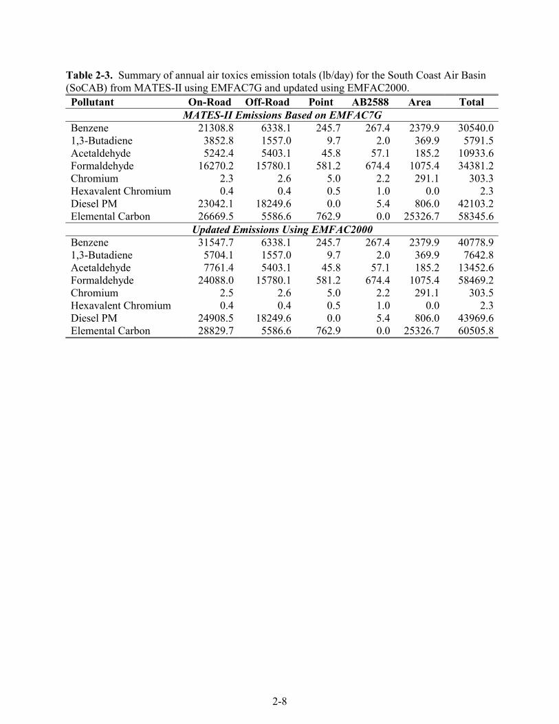
Emission Totals Table 2-3 summarizes the annual average emissions in the SoCAB for the air toxic compounds being modeled in this study. Emission totals are presented for both the MATES-II emissions inventories based on EMFAC7G and the emissions updated to EMFAC2000. The EMFAC2000 emissions update increases the on-road mobile source contributions to all air toxics. For example, the mobile source benzene contribution to total benzene emissions in the SoCAB is increased from 70% using EMFAC7G to 77% using EMFAC2000 due to the almost 50% higher VOC emissions in EMFAC2000 as compared to EMFAC7G (Table 2-2). There were smaller changes in the PM species, with on-road mobile diesel PM emissions increasing by approximately 8% (Table 2-2) for a basin-wide increase of approximately 4% (Table 2-3). The host model CB4 photochemical emissions inventory inputs were also updated to EMFAC2000 using the adjustment factors listed in Table 2-2.

2-8

Table 2-3. Summary of annual air toxics emission totals (lb/day) for the South Coast Air Basin (SoCAB) from MATES-II using EMFAC7G and updated using EMFAC2000. Pollutant On-Road Off-Road Point AB2588 Area Total

MATES-II Emissions Based on EMFAC7G Benzene 21308.8 6338.1 245.7 267.4 2379.9 30540.01,3-Butadiene 3852.8 1557.0 9.7 2.0 369.9 5791.5Acetaldehyde 5242.4 5403.1 45.8 57.1 185.2 10933.6Formaldehyde 16270.2 15780.1 581.2 674.4 1075.4 34381.2Chromium 2.3 2.6 5.0 2.2 291.1 303.3Hexavalent Chromium 0.4 0.4 0.5 1.0 0.0 2.3Diesel PM 23042.1 18249.6 0.0 5.4 806.0 42103.2Elemental Carbon 26669.5 5586.6 762.9 0.0 25326.7 58345.6

Updated Emissions Using EMFAC2000 Benzene 31547.7 6338.1 245.7 267.4 2379.9 40778.91,3-Butadiene 5704.1 1557.0 9.7 2.0 369.9 7642.8Acetaldehyde 7761.4 5403.1 45.8 57.1 185.2 13452.6Formaldehyde 24088.0 15780.1 581.2 674.4 1075.4 58469.2Chromium 2.5 2.6 5.0 2.2 291.1 303.5Hexavalent Chromium 0.4 0.4 0.5 1.0 0.0 2.3Diesel PM 24908.5 18249.6 0.0 5.4 806.0 43969.6Elemental Carbon 28829.7 5586.6 762.9 0.0 25326.7 60505.8

3-1

3. AIR TOXICS MODELING MODEL PERFORMANCE EVALUATION USING THE MATES-II DATABASE

This section presents the results for the CAMx annual air toxics model base case simulation of the MATES-II April 1998 through March 1999 year and the model performance evaluation. Results are presented for the CAMx air toxics base case simulation using EMFAC2000 mobile source emissions and standard diesel fuel. The CAMx air toxics modeling results were evaluated against the measured air toxic compound concentrations at the 10 MATES-II monitoring sites (Figure 1-2) for the following species:

• Benzene; • 1,3-Butadiene • Acetaldehyde; • Formaldehyde; • Chromium; • Hexavalent chromium; and • Elemental carbon1

Note that elemental carbon (EC) is not an air toxic compound but is used as a surrogate to assist in the evaluation of the modeling system for diesel particulate matter. A large fraction of diesel particulate matter (PM) is emitted as EC (64% according to the MATES-II report, SCAQMD 2000). Gray estimates that 67% of the EC in the SoCAB come from diesel emissions. Thus, the EC evaluation is used as a surrogate to provide an indication of the performance of the modeling system for diesel PM. Since diesel PM consists of several different components that cannot be measured separately in the atmosphere, it cannot be separately evaluated. However, it should be pointed out that gasoline combustion, vegetative burning, charboiling, and other sources also emit EC (see Table 2-3). Thus, EC is not a unique tracer species for diesel combustion. Therefore, care should be taken in using the EC performance as a quantitative measure of the model’s ability to simulate diesel PM. Model performance statistics were calculated for the seven air toxic pollutants listed above. Currently there are no model performance goals or objectives for air toxic species. The EPA UATMG Houston and Phoenix air toxic modeling demonstration studies exhibited fairly poor model performance (EPA, 1999). Whereas, the performance of the MATES-II UAM-Tox modeling ranged from fair to poor (SCAQMD, 2000). The following model performance measures were calculated in this study using the 24-hour average MATES-II observation database:

Number of Predicted/Observed Pairs: The number of predicted and observed pairs matched by time (day) and location (10 MATES-II) sites provide a measure of the robustness of the model performance statistics. Average Predicted and Observed: A comparison of the average predicted and observed values provides a measure of how well the model agrees with the observations on average.

3-2

Bias, Gross Error, and Root Mean Squared Error (RMSE): The bias, gross error, and RMSE are the average signed and unsigned (absolute value) difference and the square root of the square of the average difference in the predicted and observed concentrations in terms of µg/m3 (or ng/m3 for chromium and hexavalent chromium). Fractional Bias and Error: The fractional bias and error are presented in terms of percent and are the bias and gross error of the predicted and observed concentrations normalized by the average of the predicted and observed values. Normalized Bias and Error: The normalized bias and error are also presented in terms of percent and are the bias and gross error normalized by the observed value.

In calculating these performance statistics, no concentration thresholds were used (i.e., all predicted and observed pairs were used). Note that EPA has published ozone model performance goals for the normalized bias (≤ ± 15%) and gross error (≤ 35%) (EPA, 1991). However, the EPA ozone performance measures use an observed cutoff level that is typically 60 ppb to avoid dividing by an observed concentration near zero. As many of the air toxics compound measurements are near or close to the detection limit, then the normalized and fractional bias measures are going to exhibit much higher percentage differences than seen for ozone. Thus, we place more emphasis on the absolute measures of model performance (e.g., bias and gross error) and visual aids (e.g., scatter plots) and less on statistical measures that divide by a concentration (i.e., the fractional and normalized measures). Although there are no performance goals for air toxics modeling, Seigneur, Lohman, and Pun (2002) performed a critical review of air toxics modeling and noted uncertainties in the individual air toxics VOC species on the order of a factor of 2 or 3. MODEL PERFORMANCE EVALUATION Summary model performance statistics for each of the seven evaluation species are shown in Tables 3-1 through 3-7. Note that for the PM species (chromium, hexavalent chromium, and elemental carbon), only the fine component of the PM (PM2.5) was compared with the observed fine components because there were no observations available for the coarse (PM2.5-10) components of the species in the MATES-II observational database. Benzene Also shown in Figure 3-1 is a solid line representing the 1:1 line of perfect agreement and dotted lines representing agreement within a factor of two. Figure 3-1 displays a scatter plot of 24-hour average predicted and observed benzene concentrations for the CAMx air toxics modeling system of the MATES-II annual period. The average model benzene estimates are approximately 55% greater than the observed value. Most of the predicted and observed 24-hour benzene pairs are within a factor of 2 of each other and they are almost always within a factor of 3. The model predictions are loosely correlated with the observations with an r-squared value of 0.24.

3-3

Table 3-1. Summary model performance evaluation statistics for benzene (predicted minus observed, positive bias implies overprediction).

CAMx EMFAC2000

N 499Average Observed (µg/m3) 3.5793Average Predicted (µg/m3) 5.5540Bias (µg/m3) 1.9747Gross Error (µg/m3) 2.8501RMSE(µg/m3) 3.7184Fractional Bias (%) 51.6827Fractional Error (%) 66.5515Normalized Bias (%) 133.0869Normalized Error (%) 144.8457

Benzene CAMx EMFAC2000

0

5

10

15

20

25

0 5 10 15 20 25

Observed Concentration (µg/m3)

Pred

icte

d C

once

ntra

tion

(µg/

m3 )

?3

r2 = 0.239

Figure 3-1. Scatter plot of predicted and observed 24-hour benzene concentrations (µg/m3) with solid 1:1 line and dotted lines representing envelope of within a factor of 2.

3-4

1,3-Butadiene The model underestimates the observed average 1,3-butadiene concentrations by approximately 40% with an average observed value of approximately 1 µg/m3 and an average predicted value of approximately 0.6 µg/m3. The model fails to estimate the very highest observed 1,3-butadiene values > 3 µg/m3 as the model predictions are always under 3 µg/m3 (see Figure 3-2). This may be partly due to source-receptor impacts that are subgrid-scale to the 2-km grid resolution used in this study. The CAMx air toxics modeling system subgrid-scale point source module was not used in this application since the focus was on diesel PM impacts that are more regional in nature. In any event, the model predictions are well within the uncertainties of a factor of 2-3 reported by Seigneur and co-workers (2002).

Table 3-2. Summary model performance evaluation statistics for 1,3-butadiene (predicted minus observed, positive bias implies overprediction).

CAMx EMFAC2000

N 499Average Observed (µg/m3) 0.9987Average Predicted (µg/m3) 0.6081Bias (µg/m3) -0.3906Gross Error (µg/m3) 0.5983RMSE(µg/m3) 0.9602Fractional Bias (%) -30.0836Fractional Error (%) 71.5459Normalized Bias (%) 12.5738Normalized Error (%) 80.1203

3-5

1,3-Butadiene CAMx EMFAC2000

0

1

2

3

4

5

6

7

0 1 2 3 4 5 6 7


Pred

icte

d C

once

ntra

tion

(µg/

m3 )

3

r2 = 0.2327

Figure 3-2. Scatter plot of predicted and observed 24-hour 1,3-butadiene concentrations (µg/m3)

with solid 1:1 line and dotted lines representing envelope of within a factor of 2.

3-6

Acetaldehyde The model overestimates the average observed acetaldehyde concentration (3.0 µg/m3) by approximately 80 percent (5.6 µg/m3). A majority of the observed 24-hour acetaldehyde concentrations are reproduced to within a factor of 2 (Figure 3-3). This is in contrast to the MATES-II UAM-Tox modeling that underestimated most of the observed acetaldehyde concentrations by over a factor of 2 (SCAQMD, 2000; ENVIRON, 2002). It is interesting to note that most of the CAMx acetaldehyde estimates are above 2 µg/m3, whereas there are numerous observed values below 2µg/m3 (Figure 3-3). The reasons for this are unclear as the boundary conditions are well below 2 µg/m3 (see Table 2-1).

Table 3-3. Summary model performance evaluation statistics for acetaldehyde (predicted minus observed, positive bias implies overprediction).

CAMx EMFAC2000


3-7


Acetaldehyde CAMx EMFAC2000

0

2

4

6

8

10

12

14

16

18

20

0 2 4 6 8 10 12 14 16 18 20

Pred

icte

d C

once

ntra

tion

(µg/

m3 )

3

r2 = 0.1487

Figure 3-3. Scatter plot of predicted and observed 24-hour acetaldehyde concentrations (µg/m3) with solid 1:1 line and dotted lines representing envelope of within a factor of 2.

3-8

Formaldehyde The model simulation exhibits an overprediction tendency of the average observed formaldehyde of approximately 90% (Table 3-4). As was seen for acetaldehyde, the CAMx simulation formaldehyde estimates appear to not go below approximately 2 µg/m3 (Figure 3-4). It should be noted that formaldehyde and acetaldehyde are “lumped species” in the CB4 chemical mechanism so include other compounds besides pure formaldehyde and acetaldehyde. It should also be noted that these are also difficult species to measure and some measurement techniques will be incomplete. Thus, we would expect the model to overestimate the observed formaldehyde and acetaldehyde.

Table 3-4. Summary model performance evaluation statistics for formaldehyde (predicted minus observed, positive bias implies overprediction).

CAMx EMFAC2000


3-9

Formaldehyde CAMx EMFAC2000

0

5

10

15

20

25

30

0 5 10 15 20 25 30


Pred

icte

d C

once

ntra

tion

(µg/

m3 )

3

r2 = 0.031

Figure 3-4. Scatter plot of predicted and observed 24-hour formaldehyde concentrations (µg/m3)

with solid 1:1 line and dotted lines representing envelope of within a factor of 2.

3-10

Chromium PM2.5 The model estimates much higher average fine particulate chromium values than observed. As seen in the scatter plot in Figure 3-5, there are numerous observed PM2.5 chromium values near zero that have been set to half the detection limit when it was below the instrument detection limit. Note that because of their low concentrations, chromium and hexavalent chromium results are presented in terms of nanograms per cubic meter (ng/m3) rather than the usual micrograms per cubic meter (µg/m3) that is used for the other species (1000 ng/m3 = 1 µg/m3). The CAMx estimated average chromium concentration (12.5 ng/m3) is approximately 2.5 times the average observed value (see Table 3-5). Clearly the overprediction tendency is partly an emissions and/or measurement issue; subgrid-scale processes may also be involved. Although the CAMx air toxics modeling system model performance is poor, the CAMx overprediction (factor of 2.5) is not as severe as seen in the MATES-II UAM-Tox modeling (factor of 4.5) for chromium PM2.5 (SCAQMD, 2000; ENVIRON, 2002).

Table 3-5. Summary model performance evaluation statistics for chromium PM2.5 (predicted minus observed, positive bias implies overprediction).

CAMx EMFAC2000

N 429Average Observed (ng/m3) 4.8157Average Predicted (ng/m3) 12.5488Bias (ng/m3) 7.7331Gross Error (ng/m3) 9.7548RMSE(ng/m3) 12.7754Fractional Bias (%) 88.0641Fractional Error (%) 110.8636Normalized Bias (%) 620.7668Normalized Error (%) 637.1380

3-11

Chromium CAMx EMFAC2000

0

10

20

30

40

50

60

0 10 20 30 40 50 60


Pred

icte

d C

once

ntra

tion

(µg/

m3 )

3

r2 = 0.0009

Figure 3-5. Scatter plot of predicted and observed 24-hour chromium concentrations (µg/m3) with solid 1:1 line and dotted lines representing envelope of within a factor of 2.

3-12

Hexavalent Chromium The model also overestimates hexavalent chromium (CrVI). For CrVI, the SCAQMD and ARB laboratory equipment had two different detection limits that are readily apparent in the scatter plot as vertical lines in Figure 3-6. As shown in Table 3-6, the average observed CrVI (0.18 ng/m3) is overestimated by the CAMx air toxics modeling system by a factor of 2 (0.39 ng/m3). Note that this compares with a factor of 4 average overprediction tendency by the UAM-Tox in the MATES-II modeling (SCAAQMD, 2000; ENVIRON, 2002).

Table 3-6. Summary model performance evaluation statistics for Hexavalent Chromium PM2.5 (predicted minus observed, positive bias implies overprediction).

CAMx EMFAC2000

N 486Average Observed (ng/m3) 0.1807Average Predicted (ng/m3) 0.3874Bias (ng/m3) 0.2067Gross Error (ng/m3) 0.2944RMSE(ng/m3) 0.5162Fractional Bias (%) 34.1689Fractional Error (%) 79.4204Normalized Bias (%) 202.9212Normalized Error (%) 234.8527

3-13

Hexavalent Chromium CAMx EMFAC2000

0

0.5

1

1.5

2

2.5

3

0 0.5 1 1.5 2 2.5 3


Pred

icte

d C

once

ntra

tion

(µg/

m3 )

R2 = 0.0002

Figure 3-6. Scatter plot of predicted and observed 24-hour hexavalent chromium concentrations (µg/m3) with solid 1:1 line and dotted lines representing envelope of within a factor of 2.

3-14

Elemental Carbon The evaluation of elemental carbon (EC) is presented as a surrogate for diesel particles. However, not all EC is due to diesel combustion and not all diesel particles are EC, so the evaluation link between EC and diesel particles is purely qualitative. Furthermore, the species that make up elemental carbon may consist of other compounds and varies by measurement technique. The model exhibits fairly good model performance for EC, overpredicting the average observed EC value (3.4 µg/m3) by approximately 0.5 µg/m3 (16%) (Table 3-7). The model performance for EC is better than for the other species examined with fractional bias of about 14% (CAMx). As seen in the scatter plot in Figure 3-7, the model reproduces most of the 24-hour EC observations to within a factor of 2 and the model estimates are loosely correlated with the observations (r2 = 0.31).

Table 3-7. Summary model performance evaluation statistics for Elemental Carbon PM2.5 (predicted minus observed, positive bias implies overprediction).

CAMx EMFAC2000


3-15

Elemental Carbon CAMx EMFAC2000

0

2

4

6

8

10

12

14

0 2 4 6 8 10 12 14


Pred

icte

d C

once

ntra

tion

(µg/

m3 )

3

R2 = 0.3091

Figure 3-7. Scatter plot of predicted and observed 24-hour elemental carbon concentrations (µg/m3) with solid 1:1 line and dotted lines representing envelope of within a factor of 2.

3-16

SPATIAL DISTRIBUTION OF AIR TOXIC CONCENTRATIONS The spatial distributions of the estimated air toxic concentrations were examined for each of the species to obtain insight to the source regions and impact areas. The annual average spatial distribution of each air toxics species is presented in Appendix A. Benzene The spatial distribution of the CAMx estimated annual benzene concentrations clearly follow the major roadways in the SoCAB (Appendix A). The maximum benzene concentration of 1.1 ppb (0.0011 ppm) occurs in downtown Los Angeles at the confluence of the 5, 10, 60, and 110 freeways. From downtown Los Angeles, there are high estimated benzene concentrations heading directly west toward the coast following the 10 freeway to Santa Monica. South of Santa Monica is a more isolated benzene maximum that is centered over the LAX airport. Heading east from downtown Los Angeles, freeways 10 and 60 are clearly evident in the benzene concentration patterns as the two freeways come together in Riverside. There are also estimated elevated benzene concentrations in northern Orange County centered over Anaheim and then a trail heading east from Anaheim following freeway 91 to Riverside. The fact that the estimated benzene concentrations follow the major roadways is not surprising given that almost 80% of the benzene emissions in the SoCAB are attributable to on-road mobile sources (see Table 2-3). 1,3-Butadiene Although on-road mobile sources also dominate the 1,3-butadiene emissions in the SoCAB, contributing approximately 75% (See Table 2-3), the spatial patterns of the 1,3-butadiene concentration estimates are very different from benzene. The major feature of the CAMx estimated annual distribution of 1,3-butadiene concentrations is the presence of a blob of highest 1,3-butdiene concentrations centered over the LAX airport where annual average concentrations approaching 0.5 ppb occur. Although elevated 1,3-butadiene concentrations are seen over downtown Los Angeles and Anaheim, the peaks appear to be under 0.15 ppb and are much lower than the elevated blob over LAX of 0.25-0.50 ppb. When using a lower scale in the spatial plot (not shown), the roadways begin to appear in the 1,3-butadiene concentration distribution, but the presence of the LAX airport is still the dominant feature. The reasons why LAX is so dominant in the 1,3-butadiene concentrations distributions are unclear but are believed to be due to the following:

• Highly concentrated emissions of 1,3-butadiene from on-road and non-road (e.g., aircraft) sources;

• Coastal environment with very little vertical and horizontal mixing that limits the dispersal of pollutants;

• A highly reactive compound that decays quickly so is not transported far; and • Relatively lower photochemical oxidants on the coast as compared the interior of the

domain that result in slower 1,3-butadiene decay rates at LAX compared to further inland.

3-17

Acetaldehyde Appendix A contains spatial plots of primarily emitted and secondarily formed annual average acetaldehyde concentrations. Primary acetaldehyde concentrations have two major hot spots where annual average concentrations exceed 1 ppb: the LAX airport on the west coast near El Segundo; and the Ports of Long Beach and Los Angeles down by Long Beach. Over the rest of the SoCAB, the primary acetaldehyde concentrations are 0.5 ppb or less. The spatial distribution of secondary acetaldehyde concentrations is very different from primary acetaldehyde. Secondary acetaldehyde increases in concentrations going inland from west to east across the domain and peaking at 1-2 ppb in the Riverside/Ontario area and in the San Gabriel Mountains north of Glendora. Not surprisingly, the pattern of secondary acetaldehyde is somewhat similar to what is sometimes seen for ozone, another secondary pollutant. Appendix A also has ratios of the annual average primary to total acetaldehyde concentrations. Except for the LAX airport and port area near Long Beach, secondary acetaldehyde accounts for over 70 percent of the total acetaldehyde concentration. Eliminating LAX, the Port, and the downtown centers of Los Angeles and some of the other major cities, secondary acetaldehyde contributes 90 percent or more to the total acetaldehyde concentrations over a majority of the SoCAB. Formaldehyde LAX and the Port area are also two hot spots for primary formaldehyde concentrations where annual average concentrations of 3-8 ppb are estimated to occur (Appendix A). The city centers of Los Angeles and Anaheim are also clearly evident in the annual average primary formaldehyde spatial distribution. The gradient of secondary formaldehyde concentrations going west to east is not as pronounced as seen for acetaldehyde. The peak formaldehyde over the San Gabriel Mountains north of Glendora appears to be higher than over the Riverside/Ontario area, whereas for secondary acetaldehyde the reverse was true. This is believed to be due to the higher formaldehyde yields from biogenic VOC emissions (i.e., isoprene) that are more prevalent in the San Gabriel Mountains. The amount of primary formaldehyde to total formaldehyde is greater than seen for acetaldehyde. This is mainly because there are 4 times as much primary formaldehyde emissions as primary acetaldehyde emissions (see Table 2-3). Primary formaldehyde accounts for over 60 percent of the total formaldehyde over the LAX airport and Port regions. Away from those areas in the populated regions of the basin, primary formaldehyde accounts for 25-50% and secondary formaldehyde accounts for 50-75% of the total formaldehyde. Secondary formaldehyde dominates the total formaldehyde concentrations in the more rural and remote areas of the SoCAB.

3-18

Chromium Spatial maps of annual average fine and coarse PM chromium concentrations are contained in Appendix A. The distribution of the chromium appears to follow the roadways. The coarse mode chromium appears to be higher than the fine mode with very high concentrations out in the Riverside/Ontario/San Bernardino areas, whereas the fine mode has higher concentrations in the downtown Los Angeles area. The reasons for these differences in the spatial distribution of fine versus coarse model chromium estimates are unclear as only model-ready gridded emissions were provided so we cannot go back to the raw emissions data to identify the source categories that cause these differences. However, we do know that, as currently formulated, the fate of whether chromium resides in the fine or coarse mode is based on how it is split in the emissions inventory. The current implementation of chromium in CAMx does not allow the particles to grow and transfer from the fine to coarse modes or vice versa. The relatively high amounts of coarse mode chromium estimates raises questions regarding the adequacy of the MATES-II procedures to measure just the fine mode of this species. Hexavalent Chromium The spatial distribution of hexavalent chromium (CrVI) is very spotty and not at all related to the distributions of roadways in the SoCAB. There appears to be six isolated fine mode CrVI hot spots, five in Los Angeles and one in San Bernardino County. However, there appears to be many more (> 20) coarse mode CrVI hot spot locations. The coarse mode CrVI estimates are much greater than the fine mode CrVI estimates over most of the domain. Again, these results raise questions regarding the MATES-II approach to just make fine mode measurements to evaluate the model for a species that resides mainly in the coarse mode. If another air toxic sampling study is conducted in the SoCAB, resources should be allocated to measure coarse mode chromium and CrVI. Diesel Particles The estimated diesel particle concentrations reside almost completely within the fine PM mode (Appendix A). There are high estimated concentrations of diesel PM due to emissions from the Ports of Long Beach and Los Angeles, downtown Los Angeles, Anaheim, and areas in the Ontario/Riverside/San Bernardino area. The major roadways are evident in the diesel particle concentration estimates. However, by far the largest source region is the Port area near Long Beach where annual average concentrations in excess of 2 µg/m3 stretch from the port area to the west out to sea. The marine vessels, loading/unloading apparatus, and trucking equipment all contribute to these high diesel PM concentrations. Again, since only fully merged emissions were available, the relative contributions of these sources to the total diesel PM in the port area could not be obtained, but we suspect marine vessels to be a major contributor.

3-19

“Elemental” Carbon “Elemental” Carbon (EC) is also mainly in the fine PM mode. The spatial distributions of estimated annual average fine EC concentrations consist of five major elevated EC regions superimposed on top of elevated EC concentrations that follow the roadway distribution. The five elevated EC regions are as follows:

• The port area near Long Beach, where the EC is likely primarily due to the diesel engines in the marine vessels and support equipment;

• Downtown Los Angeles where the high EC concentrations are likely due to motor vehicle emissions from the confluence of several freeways and congestion;

• An area up in the San Gabriel Mountains that we suspect may be due to forest fires; • Around Ontario; and • Around San Bernardino.

Although there is lots of motor vehicle traffic at these latter two high EC concentration locations, it is unclear why the annual average at these two locations are higher than other major cities (e.g., Anaheim). It maybe due to a combination of high emissions, prevailing westerly winds from upwind source regions, and stagnation. Vegetative burning (wild fires) may also have played a role in these two high EC locations. The spatial distribution of the coarse EC estimates is quite different and lower than the fine EC estimates. With one notable exception, the distribution of elevated coarse EC follows the roadways. The exception is a bull’s eye annual average coarse EC approaching 2 µg/m3 that appears to occur in Upland on freeway 10 just northwest of Ontario. As only model-ready emissions files were provided by the SCAQMD, we could not investigate the details as to what in the emissions is causing this coarse EC spike at this location. SUMMARY OF MODEL PERFORMANCE The CAMx air toxics modeling system exhibited some skill in estimating the MATES-II benzene observations. The differences in the model estimates and observations were well below the uncertainties in the emissions inventory and measurements. The model exhibited an underprediction tendency for 1,3-butadiene and never estimated a 24-hour 1,3-butadiene concentration > 2 µg/m3, whereas there were over 50 observed occurrences throughout the modeling year. The CAMx reproduced the average observed acetaldehyde concentrations to within a factor of 2 with an overprediction tendency. This compares with the MATES-II UAM-Tox underprediction tendency on average by a factor of 3 (SCAQMD, 2000). Given that CAMx and UAM-Tox used basically the same chemical mechanism (CB4) and emissions, the reasons for the large differences in the CAMx and UAM-Tox acetaldehyde predictions are not known. The observed average formaldehyde is reproduced to within a factor of 2 with the model exhibiting an ~80% overprediction tendency.

3-20

For fine particulate chromium and hexavalent chromium (CrVI), the model severely overestimates the observed concentrations. The CAMx average overprediction tendency for chromium and CrVI is by a factor of approximately 2.5 and 2, respectively. This compares to the MATES-II UAM-Tox overprediction by a factor of 4.5 and 4, respectively (SCAQMD 2000; ENVIRON 2002). The model exhibits much more skill in estimating the observed elemental carbon (EC) concentrations with a bias that is within 16% of the average observed value. EC performance is used as a surrogate for model performance for diesel PM. It is fortunate that the model’s best model performance is for EC, which suggests the model diesel PM performance may be adequate which is the air pollutant we are most interested in for this study.

4-1

4. EFFECTS OF BIODIESEL FUELS ON RISK AND EXPOSURE

The CAMx air toxics modeling system was exercised for the April 1998 through March 1999 annual MATES-II period for three emission scenarios as follows:

• Standard diesel base case using EMFAC2000 mobile source emissions; • 50% penetration in the HDDV fleet of an 20%/80% biodiesel/diesel (B20) fuel; and • 100% penetration in the HDDV fleet of a B20 biodiesel fuel.

Under Task 1 of the NREL Biodiesel Air Quality and Human Health Impacts Study, Heavy Duty Diesel Vehicle (HDDV) engine test data were analyzed to determine the average effects a B20 and B100 fuel will have on tailpipe NOx, VOC, CO, and PM emissions and the toxicity of the diesel particulate matter (PM). The following results were found in regards to the diesel PM emissions from HDDV engines using a 100% biodiesel fuel (B100) and 20%/80% biodiesel/diesel (B20) fuel versus a standard petroleum based diesel fuel (Lindhjem and Pollack, 2000):

• PM emissions from HDDVs using a B20 fuel were –8.9% those of standard diesel (i.e., 8.9 percent lower);

• PM emissions from HDDVs using a B100 fuel were –55.3% those of standard diesel (i.e., 55.3 percent lower);

• PM emissions from HDDVs using a B20 fuel had –5% the toxicity of standard diesel (i.e., 5 percent lower); and

• PM emissions from HDDVs using a B100 fuel had –25% the toxicity of standard diesel (i.e., 25 percent lower).

The resultant diesel particulate matter emissions in the SoCAB for the three emission scenarios are given in Table 4-1. The 8.9 percent reduction in diesel PM from HDDVs for the 100% B20 penetration scenario results in a total reduction in diesel PM across the SoCAB of 4.7 percent. This is due to the fact that HDDV’s are estimated to contribute a little over half (52%) of the diesel PM in the SoCAB. Similarly, the approximately 4.4 percent reduction in HDDV diesel PM from the 50% B20 penetration scenario results in a SoCAB-wide reduction in diesel PM of 2.4 percent. Table 4-1. Diesel particulate matter emissions in SoCAB modeling domain for the three emission scenarios (lb/day).

100% B20 Biodiesel 50% B20 Biodiesel Source Category

Standard Diesel (lb/day) (lb/day) (%) (lb/day) (%)

HDDV 23239.6 21171.3 (-8.9) 22205.4 (-4.4)Other On-Road 1668.9 1668.9 (0.0) 1668.9 (0.0)Other Diesel 19061.1 19061.1 (0.0) 19061.1 (0.0) Total 43969.6 41901.3 (-4.7) 42935.4 (-2.4)

4-2

RISK CALCULATION AND EXPOSURE MODELING The MATES-II study used species-dependent unit risk factors (URFs) that are applied to the annual average air toxics concentrations and summed to estimate the one in a million risk of premature death due to long-term exposure to air toxics. MATES-II calculated monitored and modeled risk at the 10 MATES-II monitoring sites and averaged them to obtain the SoCAB basin-wide risk estimate. The URFs used in the MATES-II study that are also used in this study are as follows:

• Benzene: 2.9 x 10-5 (µg/m3)-1 • 1,3-Butadiene: 1.7 x 10-4 (µg/m3)-1 • Acetaldehyde: 2.7 x 10-6 (µg/m3)-1 • Formaldehyde: 6.0 x 10-6 (µg/m3)-1 • Standard Diesel Particles: 3.0 x 10-4 (µg/m3)-1

• B20 Diesel Particles: 2.85 x 10-4 (µg/m3)-1

In MATES-II, risk was calculated in terms of outdoor exposures. That is, the long-term rate of cancer incidence due to exposure to air toxics assumed that a person was outdoors 24 hours/day 365 days/year. The exposure to air toxics is going to vary greatly indoors versus outdoors by pollutant. For example, there are indoor sources of formaldehyde that increase indoor exposure to that pollutant. On the other hand, diesel PM will be greater outdoors than indoors and greater still on and near major roadways. Thus, use of solely outdoor exposures will overstate the human health benefits of biodiesel fuel use. We reviewed available literature to identify indoor/outdoor ratios that could be applied to estimate the exposure of people to outdoor air toxics. The only pollutant that was characterized sufficiently well was diesel particles, which according to MATES-II accounted for 70% of the risk in the SoCAB. Using work as reported by Hayes and co-workers (1994) we developed indoor/outdoor ratios by month and time of day that represented the following factors:

• Indoor at home; • Indoor at work; • Outdoors; and • In a car.

The resultant annual average indoor/outdoor ratio was 0.59, which agreed fairly well with the Hayes and co-workers (1994) 0.55 for adults and 0.60 for children annual indoor/outdoor ratio factors. Exposure was then calculated several different ways as follows:

4-3

• 10 site average using annual average concentrations (the MATES-II approach) and no indoor/outdoor ratio;

• 10 site average using annual average concentrations and constant annual (0.59) indoor/outdoor ratio; and

• 10 site average using hourly concentrations and hourly indoor/outdoor ratio. The results of these risk calculations for the standard diesel with and without accounting for indoor/outdoor effects are displayed in Table 4-2. When accounting for indoor/outdoor effects on diesel particles only, the estimated risk is reduced by approximately one-third. Note that there is little difference (within 2%) in the calculated risk whether a composite annual average indoor/outdoor factor is used or if hourly values are applied to the hourly air toxics concentrations. Table 4-3 compares the calculated risk in terms of a one in million risk of premature deaths due to exposure to air toxics for the standard diesel and 100% and 50% penetration of a B20 biodiesel fuel into the HDDV fleet emission scenarios. A 50% penetration of B20 in the HDDV fleet is estimated to reduce the one in a million risk of premature death due to exposure to air toxics by approximately 2 percent. A 100% penetration of a B20 fuel in the HDDV fleet is estimate to reduce the air toxics risk by approximately 5-6 percent. Table 4-2. Average risk (out of a million) of premature death due to exposure to air toxics in the SoCAB for the standard diesel scenario calculated with no indoor/outdoor (I/O) effects and accounting for indoor/outdoor effects on an annual average and hourly basis.

Scenario Risk

(Number in a million) Percent different from no

indoor/outdoor ratio. No Indoor/Outdoor Effects 1,950 Annual Indoor/Outdoor Ratio 1,284 -34.1 Hourly Indoor/Outdoor Ratios 1,257 -35.5

Table 4-3. Average risk (out of a million) of premature death due to exposure to air toxics for the standard diesel, 50% penetration of B20 in the HDDV fleet, and 100% penetration of B20 in the SoCAB in the HDDV fleet scenarios calculated with no indoor/outdoor (I/O) effects and accounting for indoor/outdoor effects on an annual average and hourly basis.

50% B20 Fuel 100% B20 Fuel Scenario

Std Diesel Risk Risk (%) Risk (%)

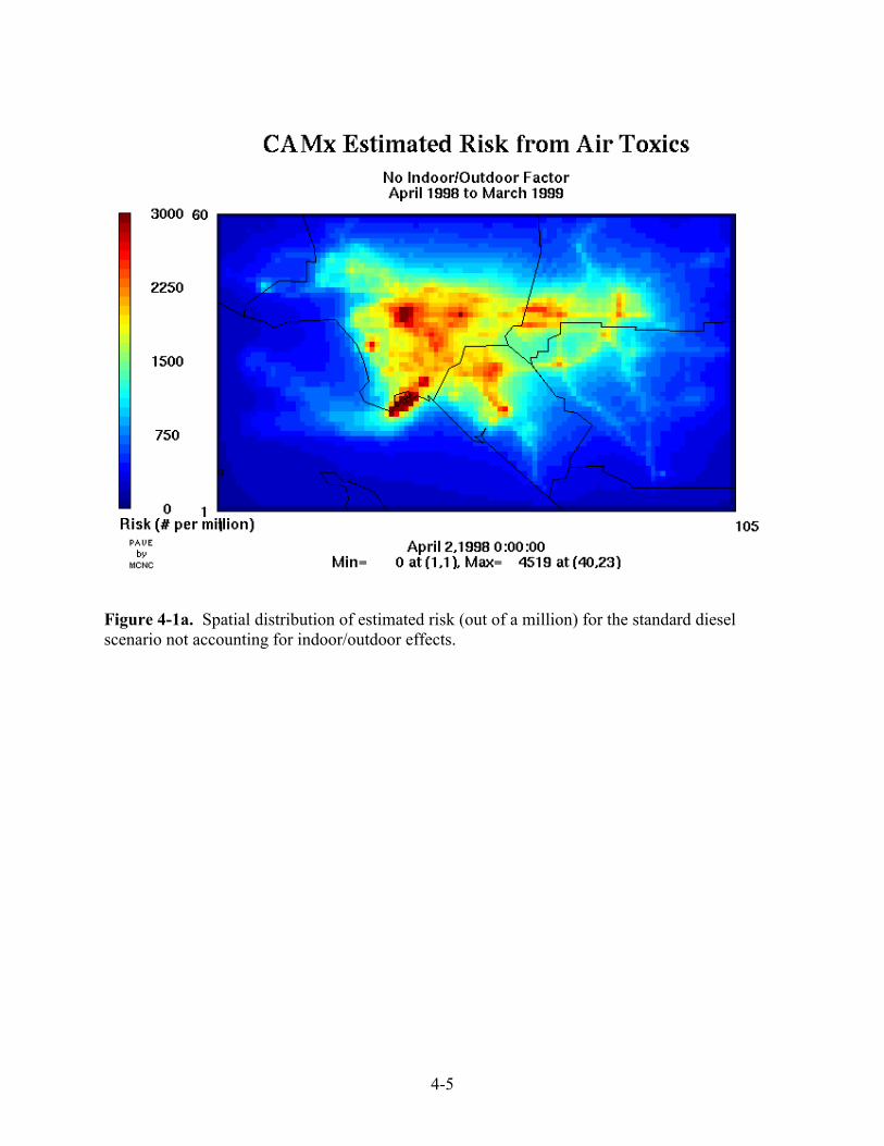
No I/O Effects 1,950 1,910 (-2.1) 1,835 (-5.9) Annual I/O Effects 1,284 1,261 (-1.8) 1,216 (-5.3) Hourly I/O Effects 1,257 1,235 (-1.8) 1,191 (-5.3) Figure 4-1 displays the spatial distribution of annual risk for the standard diesel scenario with and without accounting for indoor/outdoor effects. The highest risks occur in Los Angeles County with large areas of risk exceeding 2,000 in a million (Figure 4-1a). When indoor/outdoor

4-4

effects are accounted for there are only two isolated areas with risk exceeding 2,000 in a million, downtown Los Angeles and the port area near Long Beach. The risk at the location of the maximum risk (port area) without indoor/outdoor effects (4,519 in a million) is reduced approximately 40% when indoor/outdoor effects are accounted for (2,776 and 2,703 in a million) applying indoor/outdoor effects on an annual versus hourly basis, respectively. Combining the risk factors with population gives the exposure to air toxics. In MATES-II, the average risk and exposure across the SoCAB was estimated by applying the 10-site average risk to the basin-wide population of 14,404,993 people. Thus, the same approach is adopted here to estimate the changes in exposure due to use of biodiesel versus standard diesel fuels in the HDDV fleet. The exposure results for the standard diesel and two biodiesel fuel scenarios and the percent change in exposure due to use of a biodiesel fuel are shown in Table 4-4. The 50% penetration of a B20 biodiesel fuel into the HDDV fleet is estimated to reduce the exposure by 2.1 percent (no I/O effects) to 1.8 percent (with I/O effects). A 100% penetration of a B20 biodiesel fuel in the HDDV fleet is estimated to reduce exposure due to long-term exposure to air toxics by 5-6 percent Table 4-4. SoCAB-wide exposure (one in a million risk times population) to air toxics for the standard diesel, 50% penetration of B20 in the HDDV fleet, and 100% penetration in the HDDV fleet scenarios calculated with no indoor/outdoor (I/O) effects and accounting for indoor/outdoor effects on an annual average and hourly.

50% B20 Fuel 100% B20 Fuel Scenario

Std Diesel Exposure Exposure %Difference Exposure %Difference

No I/O Effects 28,090 27,514 2.1% 26,433 5.9% Annual I/O Effects 18,496 18,165 1.8% 17,516 5.3% Hourly I/O Effects 18,107 17,790 1.8% 17,156 5.3%

4-5

Figure 4-1a. Spatial distribution of estimated risk (out of a million) for the standard diesel scenario not accounting for indoor/outdoor effects.

4-6

Figure 4-1b. Spatial distribution of estimated risk (out of a million) for the standard diesel scenario accounting for indoor/outdoor effects on an annual basis.

4-7

Figure 4-1c. Spatial distribution of estimated risk (out of a million) for the standard diesel scenario accounting for indoor/outdoor effects on an hourly basis.

R-1

REFERENCES Calvert, J.G., R. Atkinson, K.H. Becker, R.M. Kamens, J.H. Seinfeld, T.H. Wallington and G.

Yarwood. 2002. “The Mechanisms of Atmospheric Oxidation of the Aromatic Hydrocarbons.” Oxford University Press, New York, N.Y..

Calvert, J.G., R. Atkinson, J.A. Kerr, S. Madronich, G.K. Moortgat, T.H. Wallington and G.

Yarwood. 2000. “The Mechanisms of Atmospheric Oxidation of the Alkenes.” Oxford University Press, New York, N.Y.

ENVIRON. 2002. “User’s Guide - Comprehensive Air Quality Model with Extensions

(CAMx)”. Version 3.1. (www.camx.com) April. ENVIRON. 2002. “Development, Application, and Evaluation of an Advanced Photochemical

Air Toxics Modeling System:. Prepared for Coordinating Research Council, Inc. And U.S. Department of Energy. CRC Project A-42-2. June 30.

EPA. 1999. Air Dispersion Modeling of Toxic Pollutants in Urban Areas – Guidance,

Methodology, and Example Applications. Office of Air Quality Planning and Standards. U.S. Environmental Protection Agency, Research Triangle Park, N.C. (EPA-454/R-99-021) July.

EPA. 1991. “Guidelines for the Regulatory Application of the Urban Airshed Model”. U.S.

Environmental Protection Agency, Research Triangle Park, N.C. Gray, H.S. 1986. “Control of Atmospheric Fine Primary Carbon Particle Concentrations. EQL

Report No.23, Environmental Quality Laboratory, California Institute of Technology, Pasadena, CA.

Harley R. A., and G. R. Cass. 1995, Modeling the atmospheric concentrations of individual

volatile organic compounds. Atmos. Environ. Vol. 29, No. 8, pp. 905-922. Hayes, S.R. et al. 1994. Toward Greater Realism in Air Toxics Exposure Assessment.

Presented at 88th Annual Meeting of Air & Waste Management Association, San Antonio, TX June

ICF. 2001. “User’s Guide to the Regional Modeling Systems for Aerosols and Deposition”. ICF

Consulting, Fairfax, VA. November. IUPAC. 2001. “Evaluated kinetic and photochemical data for atmospheric chemistry.” IUPAC

Subcommittee for Gas Kinetic Data Evaluation. Available at http://www.iupac-kinetic.ch.cam.ac.uk/index.html. December.

JPL. 2001. “Chemical Kinetics and Photochemical Data for Stratospheric Modeling --

Evaluation 13.” NASA Jet Propulsion Laboratory publication 00-3. Available at http://jpldataeval.jpl.nasa.gov/. February.

http://www.camx.com/

http://www.iupac-kinetic.ch.cam.ac.uk/index.html

http://www.iupac-kinetic.ch.cam.ac.uk/index.html

http://jpldataeval.jpl.nasa.gov/

R-2

Madronich, S. 2002. The Tropospheric visible Ultra-violet (TUV) model web page. http://www.acd.ucar.edu/TUV/.

Morris, R.E. et al. 2002. Evaluation of the Air Quality Impacts of Zero Emission Vehicles

(ZEVs) and a No ZEV Alternative in the South Coast Air Basin of California. Presented at Air & Waste Management Association 95th Annual Meeting and Exhibition, Baltimore, M.D.

Morris, R.E. et al. 2001. Evaluation of the Air Quality Impacts of Zero Emission Vehicles

(ZEVs) and a No ZEV Alternative in the South Coast Air Basin of California. Final Report. Prepared for C.A.T. Committee, General Motors Corporation and Toyota Motor Company. November.

Morris, R.E., K. Lee, and G. Yarwood. 1997. “Comparison of OTAG UAM-V/BEIS2 Modeling

Results with Ambient Isoprene and Other Related Species Concentrations”. ENVIRON International Corporation, Novato, CA. October.

SAI. 1999. Modeling Cumulative Outdoor Concentrations of Hazardous Air Pollutants.

Systems applications International, Inc. San Rafael, CA, SYSAPP-99-96/33r.2. February.

Scire, J.S. et al. 1999. “A User’s Guide for the CALMET Meteorological Model”. (Version 5).

Earth Tech, Concord, MA. January. SCAQMD. 2000. Multiple Air Toxics Exposure Study in the South Coast Air Basin-MATES-

II. South Coast Air Quality Management District, Diamond Bar, CA. November. Seigneur, Lohman, and Pun. 2002. “Critical Review of Air Toxics Modeling – Current Status

and Key Issues”. Atmospheric and Environmental Research, Inc. San Ramon, CA. September.

Slinn, S.A. and W.G.N. Slinn. 1980. Predictions for particle deposition on natural waters.

Atmos. Environ. Vol. 24, pp.1013-1016. Wesely, M.L. 1989. Parameterization of Surface Resistances to Gaseous Dry Deposition in

Regional-Scale Numerical Models. Atmos. Environ. 23, 1293-1304. Yarwood, G., et al. 2002. Proximate Modeling of Weekday/Weekend Ozone Differences for

Los Angeles. Draft. Prepared for Coordinating Research Council, Alpharetta, GA. May.

http://www.acd.ucar.edu/TUV/

APPENDIX A

Spatial Distribution of Annual Average Concentrations Estimated by CAMx/EMFAC2000 for:

Benzene (ppm) 1,3-Butadiene (ppm) Primary Acetaldehyde (ppm) Secondary Acetaldehyde (ppm) Primary Formaldehyde (ppm) Secondary Formaldehyde (ppm) Ratio of Primary to Total Acetaldehyde Ratio of Primary to Total Formaldehyde Chromium PM2.5 (µg/m3) Chromium PM2.5-10 (µg/m3) Hexavalent Chromium PM2.5 (µg/m3) Hexavalent Chromium PM2.5-10 (µg/m3) Diesel PM2.5 (µg/m3) Diesel PM2.5-10 (µg/m3) “Elemental” Carbon PM2.5 (µg/m3) “Elemental” Carbon PM2.5-10 (µg/m3)

REPORT DOCUMENTATION PAGE

Form Approved OMB NO. 0704-0188

Public reporting burden for this collection of information is estimated to average 1 hour per response, including the time for reviewing instructions, searching existing data sources, gathering and maintaining the data needed, and completing and reviewing the collection of information. Send comments regarding this burden estimate or any other aspect of this collection of information, including suggestions for reducing this burden, to Washington Headquarters Services, Directorate for Information Operations and Reports, 1215 Jefferson Davis Highway, Suite 1204, Arlington, VA 22202-4302, and to the Office of Management and Budget, Paperwork Reduction Project (0704-0188), Washington, DC 20503. 1. AGENCY USE ONLY (Leave blank)

2. REPORT DATE

May 2003

3. REPORT TYPE AND DATES COVERED

Subcontract Report September 1999–January 2003

4. TITLE AND SUBTITLE Impact of Biodiesel Fuels on Air Quality and Human Health: Task 5 Report, Air Toxics Modeling of the Effects of Biodiesel Fuel Use on Human Health in the South Coast Air Basin Region of Southern California 6. AUTHOR(S) R.E. Morris, Y. Jia

5. FUNDING NUMBERS

AXE-9-29079-01

7. PERFORMING ORGANIZATION NAME(S) AND ADDRESS(ES)

ENVIRON International Corporation 101 Rowland Way Novato, California 94945

8. PERFORMING ORGANIZATION

REPORT NUMBER

9. SPONSORING/MONITORING AGENCY NAME(S) AND ADDRESS(ES)

National Renewable Energy Laboratory 1617 Cole Blvd. Golden, CO 80401-3393

10. SPONSORING/MONITORING

AGENCY REPORT NUMBER NREL/SR-540-33798

11. SUPPLEMENTARY NOTES

NREL Technical Monitor: K. S. Tyson and R. McCormick 12a. DISTRIBUTION/AVAILABILITY STATEMENT

National Technical Information Service U.S. Department of Commerce 5285 Port Royal Road

Springfield, VA 22161

12b. DISTRIBUTION CODE

13. ABSTRACT (Maximum 200 words) This document is the Task 5 report for the NREL study “Impacts of Biodiesel Fuels on Air Quality and Human Health” study. The objective of Task 5 is to estimate the effects of the use of biodiesel fuels on air toxics and resultant risk, exposure, and human health.

15. NUMBER OF PAGES

14. SUBJECT TERMS biodiesel; air quality; modeling; emissions

16. PRICE CODE

17. SECURITY CLASSIFICATION

OF REPORT Unclassified


OF THIS PAGE Unclassified


OF ABSTRACT Unclassified

20. LIMITATION OF ABSTRACT

UL

NSN 7540-01-280-5500 Standard Form 298 (Rev. 2-89) Prescribed by ANSI Std. Z39-18 298-102

impact of biodiesel fuels on air quality and human … toxics modeling model performance evaluation...

Documents