Iv

La

b

a

ARA

KIIAN

1

vfiapfudia

aUnpcgdfasfl

0d

Optik 123 (2012) 1177– 1182

Contents lists available at ScienceDirect

Optik

jou rna l homepage: www.elsev ier .de / i j leo

maging deviation through non-uniform flow fields around high-speed flyingehicles

iang Xua,b, Yuanli Caia,∗

School of Electronic and Information Engineering, Xi’an Jiaotong University, No.28 Xianning West Road, Xi’an 710049, ChinaSchool of Information Science and Engineering, Xinjiang University, No. 14 Shengli Road, Urumqi 830046, China

r t i c l e i n f o

rticle history:eceived 24 February 2011ccepted 14 July 2011

a b s t r a c t

The non-uniform flow field around high-speed flying vehicle “bends” the ray and imposes a deviationat the end of the propagation path. This imaging deviation is a kind of aero-optic effect. In this paper,we catalog the factors that influence the deviation into two classes: the vehicle-related factors and theflowfield-related factors. Flow density computation and density–refractive index conversion are dis-

eywords:magingmaging deviationero-opticson-uniform flow field

cussed. A backward ray-tracing scheme is proposed. The deviations, the propagation path distances inthe non-uniform flow field, and the density distributions along propagation paths for two different flyingcases are computed. Three flowfield-related factors should be considered in order to reduce the devia-tion: the propagation path distance in the non-uniform flow field, which should be as short as possible;the angle of incidence at the freestream boundary, which should be as small as possible; and the densitydistribution along propagation path in the non-uniform flow field, which should be as flat as possible.

. Introduction

There is a non-uniform flow field around the high-speed flyingehicle traveling through the atmosphere. This non-uniform floweld behaves as a strong optical/infrared lens. It “bends” the raynd imposes an imaging deviation at the end of the propagationath. In order to obtain better aerodynamic and aero-optic per-ormances, the vehicles with optical/infrared imaging systems aresually designed to be with conical head and side-mounted win-ow [1]. However, the imaging deviations still seriously affect the

maging applications, e.g., positioning, targeting, detection, homingnd tracking [2–4].

The flow field around high-speed flying vehicle has the char-cters of high temperature, high pressure and high turbulence.nlike many regular gradient-index mediums, this flow field haso analytical expression for the refractive index distribution. Inrevious researches, experimental techniques [5] and theoreti-al approaches including Fourier optics [6], wave optics [7] andeometrical optics [2,8–10], combined with computational fluidynamics [2,4,6–13], were employed to evaluate the optical per-ormances, and investigate the relationships between the deviation

nd the influencing factors such as altitude and angle of attack. Ithould be noted that the deviation originates in the non-uniformow field. However, altitude and angle of attack do not directly

∗ Corresponding author. Tel.: +86 29 82664113; fax: +86 29 82664113.E-mail addresses: ylicai@mail.xjtu.edu.cn, alvinlxu@gmail.com (Y. Cai).

030-4026/$ – see front matter © 2011 Elsevier GmbH. All rights reserved.oi:10.1016/j.ijleo.2011.07.046

© 2011 Elsevier GmbH. All rights reserved.

characterize the properties of the non-uniform flow field, and theyare the state variables that characterize the vehicle. Therefore, thesevehicle-related factors such as altitude and angle of attack do notdirectly influence the deviation. The cause for the deviation vary-ing with these vehicle-related factors is that the variations of thesefactors have triggered some physical variables that relate to theorigin of the deviation, viz. the non-uniform flow field. In otherwords, the vehicle-related factors are the indirect causes for thevariation of the deviation, and the flowfield-related factors are thedirect causes. Therefore, only studying the relationship betweenthe deviation and the vehicle-related factors is not enough, it isnecessary to further investigate the flowfield-related factors.

Studying the flowfield-related factors that influence the imagingdeviation, on the one hand, is helpful for understanding the opti-cal/infrared imaging through the non-uniform flow field aroundhigh-speed flying vehicle. On the other hand, with the purpose ofreducing the deviation, this study provides useful information forvehicle control, on-board optical/infrared system design, operationand compensation. For example, altitude, angle of attack and atti-tude angles (pitch, yaw and roll angle) can be adjusted from theperspective of vehicle control; the vehicle’s shape and the refractiveindex distribution can be used to adjust the window installation andlayout from the perspective of optical/infrared system design; andthe line-of-sight (LOS) angle can be adjusted from the perspective

of optical/infrared system operation. In addition, the control, designand operation variables usually do not independent. For example,the LOS angle is coupled to the attitude angles; and the windowlayout is also coupled to the attitude angles to make sure the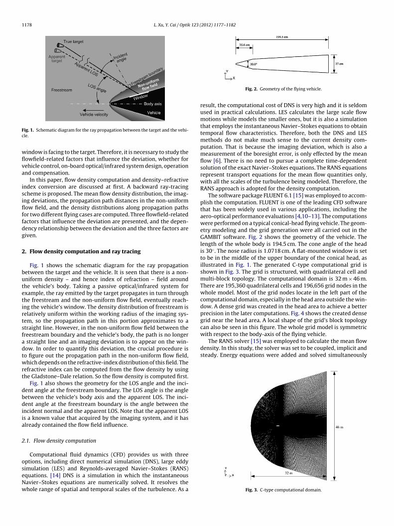

1178 L. Xu, Y. Cai / Optik 123 (2012) 1177– 1182

Fc

wflva

isiflffdg

2

butetirtsfadtwrt

dbdiia

2

oseNw

The RANS solver [15] was employed to calculate the mean flowdensity. In this study, the solver was set to be coupled, implicit andsteady. Energy equations were added and solved simultaneously

ig. 1. Schematic diagram for the ray propagation between the target and the vehi-le.

indow is facing to the target. Therefore, it is necessary to study theowfield-related factors that influence the deviation, whether forehicle control, on-board optical/infrared system design, operationnd compensation.

In this paper, flow density computation and density–refractivendex conversion are discussed at first. A backward ray-tracingcheme is proposed. The mean flow density distribution, the imag-ng deviations, the propagation path distances in the non-uniformow field, and the density distributions along propagation paths

or two different flying cases are computed. Three flowfield-relatedactors that influence the deviation are presented, and the depen-ency relationship between the deviation and the three factors areiven.

. Flow density computation and ray tracing

Fig. 1 shows the schematic diagram for the ray propagationetween the target and the vehicle. It is seen that there is a non-niform density – and hence index of refraction – field aroundhe vehicle’s body. Taking a passive optical/infrared system forxample, the ray emitted by the target propagates in turn throughhe freestream and the non-uniform flow field, eventually reach-ng the vehicle’s window. The density distribution of freestream iselatively uniform within the working radius of the imaging sys-em, so the propagation path in this portion approximates to atraight line. However, in the non-uniform flow field between thereestream boundary and the vehicle’s body, the path is no longer

straight line and an imaging deviation is to appear on the win-ow. In order to quantify this deviation, the crucial procedure iso figure out the propagation path in the non-uniform flow field,hich depends on the refractive-index distribution of this field. The

efractive index can be computed from the flow density by usinghe Gladstone–Dale relation. So the flow density is computed first.

Fig. 1 also shows the geometry for the LOS angle and the inci-ent angle at the freestream boundary. The LOS angle is the angleetween the vehicle’s body axis and the apparent LOS. The inci-ent angle at the freestream boundary is the angle between the

ncident normal and the apparent LOS. Note that the apparent LOSs a known value that acquired by the imaging system, and it haslready contained the flow field influence.

.1. Flow density computation

Computational fluid dynamics (CFD) provides us with threeptions, including direct numerical simulation (DNS), large eddy

imulation (LES) and Reynolds-averaged Navier–Stokes (RANS)quations. [14] DNS is a simulation in which the instantaneousavier–Stokes equations are numerically solved. It resolves thehole range of spatial and temporal scales of the turbulence. As a

Fig. 2. Geometry of the flying vehicle.

result, the computational cost of DNS is very high and it is seldomused in practical calculations. LES calculates the large scale flowmotions while models the smaller ones, but it is also a simulationthat employs the instantaneous Navier–Stokes equations to obtaintemporal flow characteristics. Therefore, both the DNS and LESmethods do not make much sense to the current density com-putation. That is because the imaging deviation, which is also ameasurement of the boresight error, is only effected by the meanflow [6]. There is no need to pursue a complete time-dependentsolution of the exact Navier–Stokes equations. The RANS equationsrepresent transport equations for the mean flow quantities only,with all the scales of the turbulence being modeled. Therefore, theRANS approach is adopted for the density computation.

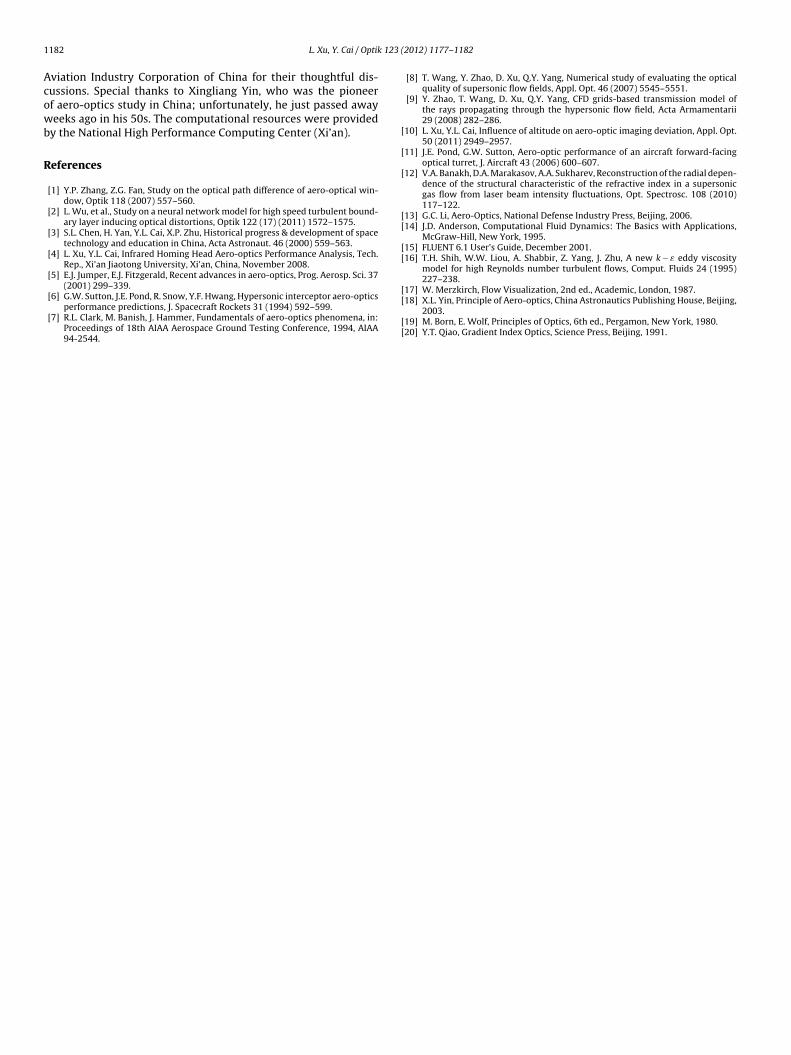
The software package FLUENT 6.1 [15] was employed to accom-plish the computation. FLUENT is one of the leading CFD softwarethat has been widely used in various applications, including theaero-optical performance evaluations [4,10–13]. The computationswere performed on a typical conical-head flying vehicle. The geom-etry modeling and the grid generation were all carried out in theGAMBIT software. Fig. 2 shows the geometry of the vehicle. Thelength of the whole body is 194.5 cm. The cone angle of the headis 30◦. The nose radius is 1.0718 cm. A flat-mounted window is setto be in the middle of the upper boundary of the conical head, asillustrated in Fig. 1. The generated C-type computational grid isshown in Fig. 3. The grid is structured, with quadrilateral cell andmulti-block topology. The computational domain is 32 m × 46 m.There are 195,360 quadrilateral cells and 196,656 grid nodes in thewhole model. Most of the grid nodes locate in the left part of thecomputational domain, especially in the head area outside the win-dow. A dense grid was created in the head area to achieve a betterprecision in the later computations. Fig. 4 shows the created densegrid near the head area. A local shape of the grid’s block topologycan also be seen in this figure. The whole grid model is symmetricwith respect to the body-axis of the flying vehicle.

Fig. 3. C-type computational domain.

L. Xu, Y. Cai / Optik 123 (2012) 1177– 1182 1179

Fig. 4. Computational grid near the head.

Table 1Vehicle conditions.

Vehicle conditions Case 1 Case 2

Altitude 30 km 40 kmMach number 3 6Angle of attack 2◦ 4◦

Table 2Freestream conditions.

Freestream conditions Case 1 Case 2

Gauge pressure 1197 Pa 287.14 Pa

waetsouaa

adpsit

Temperature 226.509 K 250.35 KDensity 1.8410 × 10−2 kg/m3 3.9957 × 10−3 kg/m3

ith the flow equations. The realizable k − ε model [15,16] wasdopted to model the turbulence. It is a two-equation model thatmploys partial differential equations to govern the transport ofhe turbulent kinetic energy, k, and its dissipation rate, ε. Thetandard wall functions [15] were adopted to handle the interfacef the flow field with the surface of the flying vehicle. Second-orderpwind scheme was employed to discretize the flow equationsnd the QUICK [15] scheme was used for turbulence kinetic energynd turbulence dissipation rate.

Two cases were simulated in this study. The vehicle conditionsre specified in Table 1, and the corresponding freestream con-itions are in Table 2. At these conditions, the simulations wereerformed and the mean flow results were acquired. Figs. 5 and 6

how the density contour for cases 1 and 2, respectively. Note thatn most scenarios, the vehicle is flying towards the target side, sohe window has to stay in the up-wind side of the vehicle so as to

Fig. 5. Mean flow density contour of case 1.

Fig. 6. Mean flow density contour of case 2.

“see” the target. Therefore the flow directions in Figs. 5 and 6 areset to be from top lefts to down rights, and the coordinates in thesetwo figures are the CFD computation coordinates, while not otherreference frames used in the true scenarios.

2.2. Density–refractive index conversion and backward raytracing

The density field computed by CFD needs to be converted intothe refractive index field. The Lorentz–Lorenz equation, also knownas Maxwell’s formula, relates the refractive index of a substance toits polarizability. It can be written in the form [17]

n2 − 1n2 + 2

= 2�

3KGD (1)

where n is the index of refraction, � is the density, KGD is theGladstone–Dale coefficient. In the infrared region, KGD is weaklydependent on the wavelength and can be approximately expressedby [18]

KGD(�) = 2.23 × 10−4

(1 + 7.52 × 10−3

�2

)(2)

In this study, the imaging sensor was considered to be InSb,which sensitive to wavelengths of 3–5 �m, so a 4-�m wavelengthwas computed.

Since the refractive index of air is approximately equal to 1,substituting n2 + 2 ≈ 3 and n2 − 1 = (n + 1)(n − 1) into Eq. (5), theGladstone–Dale relation can be obtained by the following:

n − 1 = �KGD (3)

Eq. (3) provides a bridge linking the density, an aerodynamic vari-able, to the index of refraction, an optics variable. After the densityfield was mapped into the index-of-refraction field, ray tracingwould be carried out within the field.

Differing from previous ray-tracing scheme that performed trac-ing in a preset mesh region, we discarded the preset mesh andreversed the tracing system, videlicet, started the tracing from thewindow and ended it at the freestream boundary. As comparedto the previous scheme, the advantage of this backward tracingscheme is that it performs tracing in an open direction facing to thefreestream, no longer a closed direction facing to the window. So itdoes not need to preset the scope of tracing or analyze the refrac-tive index distribution before ray tracing. The backward ray-tracingscheme was carried out by solving the ray equation [19][ ]

dds

n(r)drds

= ∇n(r), (4)

where r is the position vector of a point on the ray path, n representsthe refractive index distribution and ds is a small step along the

1180 L. Xu, Y. Cai / Optik 123 (2012) 1177– 1182

ru

RT

T

w

t

T

s

R

D

s

⎧⎪⎨⎪⎩w⎧⎪⎪⎪⎨⎪⎪⎪⎩

Bseespd

Fig. 7. Deviation versus LOS angle.

ay path. This equation specifies the relationship between the non-niformity of the medium and the change in the ray path.

The ray equation was numerically resolved using theunge–Kutta method [20]. At the beginning, an optical ray vector

is defined as

= ndrds

= drdt

(5)

here t is a new parameter defined by

=∫

ds

n, dt = ds

n(6)

hen Eq. (4) is written as

d2rdt2

= n∇n = 12

∇n2 (7)

For a 2D study Eq. (7) has two components, and they are solvedimultaneously by using two-element 1D arrays that defined by

=(

xy

), T =

(Tx

Ty

)= n

(dx/dsdy/ds

), and

= n

(∂n/∂x∂n/∂y

)= 1

2

(∂n2/∂x∂n2/∂y

)(8)

o Eq. (6) is written as the matrix form:

d2R

dt2= D(R) (9)

Then the recursive equations are obtained as follows:

Rn+1 = Rn + �t[

Tn + 16

(A + 2B)]

Tn+1 = Tn + 16

(A + 4B + C)

(10)

here the matrices A, B and C are defined as

A = �tD(Rn)

B = �tD(

Rn + �t

2Tn + 1

8�tA

)

C = �tD(

Rn + �tTn + 12

�tB) (11)

In the preceding equations, �t is the incremental value of t.ased on this method, the ray was traced step by step from thetarting point to the next location within the computed flow-field,ventually reaching the end point at the freestream boundary. Then

xtending the ray back to the window and comparing the inter-ecting point with the starting point, the distance between the twooints is the desired deviation. Fig. 7 shows the computed imagingeviations of cases 1 and 2, for LOS angles ranging from 0◦ to 60◦

Fig. 8. Propagation path distance versus LOS angle.

with a 5◦ step length. It is seen that the deviation decreases as LOSangle increases.

3. Imaging deviation and flowfield-related factors

Three flowfield-related factors that influence the imaging devi-ation are extracted. The first factor is the propagation path distancethrough the non-uniform flow field. As shown in Fig. 1, consider apassive system, the propagation path in the non-uniform flow fieldstarts from the freestream boundary and ends at the window. Theshock wave area, which is close to the freestream boundary, has themost significant density and density gradient. But the near-windowarea has smaller density and density gradient. If we divide the prop-agation path into two segments: the upper one that starts from thefreestream boundary and ends at the shock wave, and the lowerone that starts from the shock wave and ends at the window, it isof note that the deflection angle on the upper segment is greaterthan that on the lower one. Given a fixed deflection angle and max-imum density at the upper segment in the same non-uniform flowfield, the longer the propagation distance is, the larger the devi-ation will be. The 0◦ LOS-angle case has the longest propagationdistance through the non-uniform flow field, so it will induce thelargest deviation. In order to validate this analysis, the propaga-tion path distances of cases 1 and 2 for LOS angles from 0◦ to 60◦

with a 5◦ step length are investigated, and the results are shownin Fig. 8. It is seen that as the LOS angle increases, the propaga-tion path distance decreases. Therefore, a larger propagation pathdistance through the same non-uniform flow field induces a largerimaging deviation.

The second factor is the angle of incidence at the freestreamboundary. As illustrated in Fig. 9(a), an equivalent refractive planecan be assumed using the geometrical optics concept. The ray pass-ing through the refractive plane will deflect a certain angle. It iseasy to prove by optics knowledge that smaller angle of incidencewill induce smaller deflection angle, as illustrated in Fig. 9(a): if theangle of incidences ˛ > �, then the deflection angles (˛ − ˇ) > (� − �).Fig. 9(b) illustrates the relationship between the deflection angleand the deviation: if the deflection angles ( ̨ − ˇ) > (� − �), then thedeviations AB > CD. For a fixed propagation path distance d, thesmaller the deflection angle is, the smaller the deviation will be.Therefore, as the angle of incidence decreases, the deflection angledecreases and hence the imaging deviation decreases. The angleof incidence reaches maximum at the 0◦ LOS-angle case, so theimaging deviation also reaches maximum in that case.

The third factor is the density distribution along the propagation

path in the non-uniform flow field. The density of the non-uniformflow field is high in the shock wave area and low in the near-window area. When the ray propagates in the non-uniform flowfield, the density along the ray path will first raise then decline.

L. Xu, Y. Cai / Optik 123 (2012) 1177– 1182 1181

Fig. 9. Relationship between (a) the angle of incidence ( ̨ and �) and the deflectionaC

AaFfiptddofatflg

Fo

ngle (( ̨ − ˇ) and (� − �)), and (b) the deflection angle and the deviation (AB andD).

lthough for different LOS angles the trends of density variationsre the same, the flatness of density distributions are still different.or smaller LOS angle, the ray pierces into the non-uniform floweld at its foreside, where the density distribution along the rayath is sharper; while for larger LOS angle, the ray pierces intohe non-uniform flow field at its downside, where the densityistribution along the ray path is flatter. Fig. 10 shows the densityistribution along propagation path in the non-uniform flow fieldf case 1. Fig. 10(a)–(f) are the density distributions for LOS anglesrom 0◦ to 50◦, 10◦ step length. The symbol � represents the distancelong propagation path from the window. The normalization fac-ors ı0–ı50 are the propagation path distances in the non-uniform

ow field for 0–50◦ LOS-angles, respectively. It is seen that thereater the LOS angle, the flatter the density distribution. Therefore,

ig. 10. Density distribution along propagation path in the non-uniform flow fieldf case 1.

Fig. 11. Density distribution along propagation path in the non-uniform flow fieldof case 2.

larger LOS angle induces smaller bend of ray and hence smallerimaging deviation. Similar results for case 2 are shown in Fig. 11.

4. Conclusions

The imaging deviation through non-uniform flow field aroundhigh-speed flying vehicle has been studied. The factors that influ-ence the imaging deviation were cataloged into two classes: (1)vehicle-related factors, such as altitude, angle of attack, LOS angleand attitude angle; and (2) flowfield-related factors, including thepropagation path distance through the non-uniform flow field, theangle of incidence at the freestream boundary and the density dis-tribution along the propagation path. It is found that in order toreduce the imaging deviation, the propagation path distance in thenon-uniform flow field should be as short as possible; the angle ofincidence at the freestream boundary should be as small as possi-ble; and the density distribution along the propagation path in thenon-uniform flow field should be as flat as possible.

Studying the dependency relationship between the imagingdeviation and the vehicle’s state variable is in the image qualityassessment phase, so it only accounts for the vehicle that has afixed configuration. However, studying the dependency relation-ship between the deviation and the flowfield-related factors canbe in the optical/infrared system design phase. So this study is notonly helpful in understanding the optical/infrared imaging throughthe non-uniform flow field around high-speed flying vehicles, butalso in deviation–reduction-motivated vehicle control, on-boardoptical/infrared system design, operation and compensation.

Acknowledgments

The authors thank Yaolei Zhang, Guoqiang Shi and GuangchunZhang from R&D Center of China Academy of Launch Vehicle Tech-nology, Peng Shi from Xi’an Jiaotong University, and Zhe Liu from

1 123 (

Acowb

R

[

[

[

[[

[[

182 L. Xu, Y. Cai / Optik

viation Industry Corporation of China for their thoughtful dis-ussions. Special thanks to Xingliang Yin, who was the pioneerf aero-optics study in China; unfortunately, he just passed awayeeks ago in his 50s. The computational resources were provided

y the National High Performance Computing Center (Xi’an).

eferences

[1] Y.P. Zhang, Z.G. Fan, Study on the optical path difference of aero-optical win-dow, Optik 118 (2007) 557–560.

[2] L. Wu, et al., Study on a neural network model for high speed turbulent bound-ary layer inducing optical distortions, Optik 122 (17) (2011) 1572–1575.

[3] S.L. Chen, H. Yan, Y.L. Cai, X.P. Zhu, Historical progress & development of spacetechnology and education in China, Acta Astronaut. 46 (2000) 559–563.

[4] L. Xu, Y.L. Cai, Infrared Homing Head Aero-optics Performance Analysis, Tech.Rep., Xi’an Jiaotong University, Xi’an, China, November 2008.

[5] E.J. Jumper, E.J. Fitzgerald, Recent advances in aero-optics, Prog. Aerosp. Sci. 37(2001) 299–339.

[6] G.W. Sutton, J.E. Pond, R. Snow, Y.F. Hwang, Hypersonic interceptor aero-opticsperformance predictions, J. Spacecraft Rockets 31 (1994) 592–599.

[7] R.L. Clark, M. Banish, J. Hammer, Fundamentals of aero-optics phenomena, in:Proceedings of 18th AIAA Aerospace Ground Testing Conference, 1994, AIAA94-2544.

[[

[[

2012) 1177– 1182

[8] T. Wang, Y. Zhao, D. Xu, Q.Y. Yang, Numerical study of evaluating the opticalquality of supersonic flow fields, Appl. Opt. 46 (2007) 5545–5551.

[9] Y. Zhao, T. Wang, D. Xu, Q.Y. Yang, CFD grids-based transmission model ofthe rays propagating through the hypersonic flow field, Acta Armamentarii29 (2008) 282–286.

10] L. Xu, Y.L. Cai, Influence of altitude on aero-optic imaging deviation, Appl. Opt.50 (2011) 2949–2957.

11] J.E. Pond, G.W. Sutton, Aero-optic performance of an aircraft forward-facingoptical turret, J. Aircraft 43 (2006) 600–607.

12] V.A. Banakh, D.A. Marakasov, A.A. Sukharev, Reconstruction of the radial depen-dence of the structural characteristic of the refractive index in a supersonicgas flow from laser beam intensity fluctuations, Opt. Spectrosc. 108 (2010)117–122.

13] G.C. Li, Aero-Optics, National Defense Industry Press, Beijing, 2006.14] J.D. Anderson, Computational Fluid Dynamics: The Basics with Applications,

McGraw-Hill, New York, 1995.15] FLUENT 6.1 User’s Guide, December 2001.16] T.H. Shih, W.W. Liou, A. Shabbir, Z. Yang, J. Zhu, A new k − ε eddy viscosity

model for high Reynolds number turbulent flows, Comput. Fluids 24 (1995)227–238.

17] W. Merzkirch, Flow Visualization, 2nd ed., Academic, London, 1987.18] X.L. Yin, Principle of Aero-optics, China Astronautics Publishing House, Beijing,

2003.19] M. Born, E. Wolf, Principles of Optics, 6th ed., Pergamon, New York, 1980.20] Y.T. Qiao, Gradient Index Optics, Science Press, Beijing, 1991.