Image guided failure assessment using 2D displacement Tracking algorithms

Progress Report (May – July 2005)

Girish Kr. Singhal

Institute for Biomedical Engineering

ETH & University of Zurich

Supervisor : Dr. Jess Snedeker

• Objective : To map local strains in biological tissues , and predict faliure thereof

• Approach : The tissue under consideration is clamped in the universal test machine and cycles of known stress is applied.

Unlike Rubber , Biological tissues like tendons in Rat Tail , display uneven strain fields and are supposed to be kept in saline solution while under observation.

Basic requirement :

• We need to sectorize the image into small windows , whose displacements would be mapped in a sequence of images taken at regular interval of time during the entire stress cycle.

•To map the displacement undergone by a window , we need to accurately locate the test window in the next frame (deformed).

•This requires presence of some distinguishing features in the window , which can help in precisely locating the position of the window after deformation.

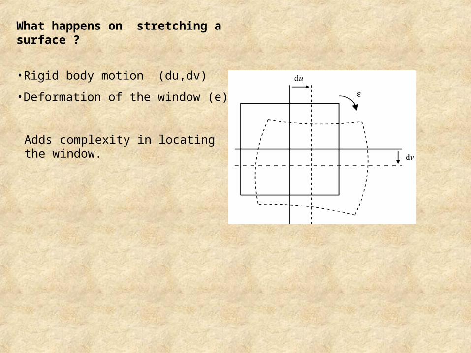
What happens on stretching a surface ?

•Rigid body motion (du,dv)

•Deformation of the window (e)

Adds complexity in locating the window.

Need for Contrast

White light Laser light

Laser speckle image white light speckle image

white light Speckle image:

Applying a powder or paint speckle to the surface of the sample.

Problem : smallest physically achievable speckles , on magnification (required due to small size of tissues , 2mm*2mm) , becomes very huge.

Laser speckle experiments, far easy to conduct , size of speckle governed by F-Stop number , It‘s an optical phenomena and not physical.

Parametres

•size of window (typical size 33*33 pixels)

•Size of features (around 5*5 pixels each)

A function of camera aperture and magnificationSmall speckle (high spatial resolution) vs. large speckle (easier to track)

one feature should be about 3 × 3 pixels and several features per subregion are required to ensure correlation..Higher the number of features , lower is the uncertainityin the displacement calculation.However good spatial resolution limits the size of window.

More on Displacement accuracies is discussed later on.

Once we have the contrast , we can use any displacement tracking algorithm , most popularls used is 2D image correlation.

256 * 256 laser speckle image

C = ifft2 ( fft2 (A) * fft2( B ))

Where fft2 and ifft2 are 2D fourier and inverse fourier tranform.

2D Correlation

2D and 3D

• For 3D strains mapping , An indisposable step is to find a precise 2D Strain mapping tool.

To find out of plane strains in 3D laser experiments.

For inplane Displacements , simple 2D Speckle tracking Algorithm reqd.

Once we have the contrast ready

•Sterio-scopy helps in Stereo-correlation using epipolar geometry (post rectification)•Temporal correlation .

3D White light Speckle tracking

•Either Sterio-triangulation formuales , or pattern recognition machines like ANN may be used to find 3D corrdinates , out of pair of 2D coordinates.

•ANNs , helps in getting rid of complex process of camera callibration at the cost of accuracies.

Artificial Speckle simulator

•To test algorithms for known displacements ,practically impossible to validate local strain maps with experimental data.Need physical markers on surface to do so.

•Method proposed by Huntley (1) has been adopted .

Modelling parametres :

•Size of the speckle image ( m,n )

•Rigid body translations ( kx , ky)

•Decorrelation factor ( delta )

•Speckle density and size ( D )

D = 100 D = 75 D = 50

Principle :

•Plane 1 : pupil plane of the lens A1(m1,n1)•Plane 2 : detector A2(m2,n2)

• A2 = randn(m,n) the amplitude of the speckle pattern incident on the detector in the absence of a lens

•A1 = fft2(A2) The effect of the lens is produced by simple fourier transformation to plane 1

•To add the effect of aperture of lense

•To displace value of speckle at each row by km and col by kn

A decorrelated Speckle movies generated from simulator

2D Laser speckled Image Tracking

Limiting issues

1) Problem of Decorrelation : Causes frame to frame flickering of pixel values (waxing and waning of intensity)

Normalising the entire image to common Mean and variance. (preprocessing step)

2) Deformation of window :Increasing the frame rate(fps) helps , cant increase indefinately , calls for very accurate SPA , introduces randomness in the algo.

3) Correlation is very erractic in nature : we need more intelligent decision maker….current area of research…

More on it soon….

Limiting issues ..cont..

4) Unlike Rubber , Biological tissues like tendons in Rat Tail , display uneven strain fields and are supposed

to be kept in saline solution while under observation .They even has high tendency to deform.

5) For a typical window size of 33 pixels , 5% strains calls for a total change in length of around 1.5 pixels over around 300 frames .This demands very high sub pixel accuracies (SPA)

Fourier Interpolation Used.

Algorithm

Step 1: Defining sequence

Frame 670 Frame 970

Step 2: Defining ROI and sectorising the entire image in windows

Parametres :

•ROI (see the movie and crop the area)

•length of window (tlen) , should have sufficient features to unambiguously locate the window in the image

Parametres :

Averaging : filter order (3*3)

Normalisation : mean(Mo) , variance(Vo) , sect

Helps in tackling with decorrelation problem quite well

Show the rectified normalised movie

At 0 to max scale At 0 to 255 scale

Step 3: Preprocessing using Averaging followed by sector wise normalisation

Scaled decorrelated image averaged decorrelated image normalised image

Mi , Vi are mean and variance of the sector I(x,y) belong to

Before pre -processing

After pre-processing

Compare decorrelated and pre processed speckle movies

Step 4 : Cross correlation using mycorr

•Correlates only in the quadrant where displacement is expected , learned from previous correlation

•Syntax :

C(x,y) = mycorr1(template,image,P,quad num)

Parametres :

• P : is the number of points at which cross correlation is computed.

• Value of P , is chosen in accordance with the next Step of interpolation

•If using prev quad num , gives very low max corr value , then redo correlation with with entire nbd.

0 2 4 6 8 10 12010

20-0.2

0

0.2

0.4

0.6

0.8

1

1.2

Step 5 :Fourier Interpolation of cross correlation values

•Interframe displacements are sub-pixular , thus interpolation of cross correlated values are unavoidable.

•Popular techniques : Cubic splines , Biparabolic fits

•Since c(x,y) is inverse fourier tranformed

Parametre :

•res , increases the computation cost quadratically.

• adist , governs the search area , we expect that Interframe displacement would be withen 1 pixel , thus adist is chosen 1 pixel.

45

6

44.555.56

0.55

0.6

0.65

0.7

0.75

0.8

0.85

0.9

0.95

1

Syntax : interpolate2(cross corr image,x,y)

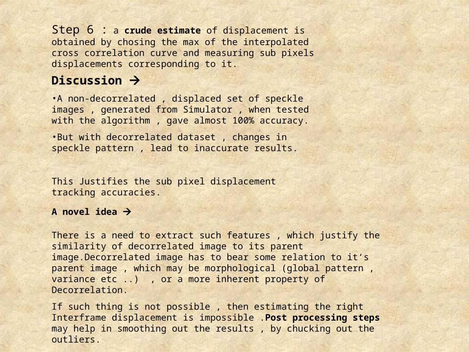
Step 6 : a crude estimate of displacement is obtained by chosing the max of the interpolated cross correlation curve and measuring sub pixels displacements corresponding to it.

A novel idea

There is a need to extract such features , which justify the similarity of decorrelated image to its parent image.Decorrelated image has to bear some relation to it‘s parent image , which may be morphological (global pattern , variance etc ..) , or a more inherent property of Decorrelation.

If such thing is not possible , then estimating the right Interframe displacement is impossible .Post processing steps may help in smoothing out the results , by chucking out the outliers.

Discussion •A non-decorrelated , displaced set of speckle images , generated from Simulator , when tested with the algorithm , gave almost 100% accuracy.

•But with decorrelated dataset , changes in speckle pattern , lead to inaccurate results.

This Justifies the sub pixel displacement tracking accuracies.

Suppose the expected displacement is (11 ,14)

(10,14) (10,15) (10,16)

(11,14) (11,15) (11,16)

(12,14) (12,15) (12,16)

(13,14) (13,15) (13,16)

Average of the displacements (independently in X and Y direction ) corresponding to top 9 values always results in the disp correponding to the highest corr val.

Thus averging the displacements doesnt give us the actual displacement.This call for feature Extraction.

Step 7 : We choose top 9 interpolated correlated curve values , as expected , these correspond to close nbd of the top value

Using these 9 displacement values , 9 images are reconstructed from Image A , based on the following assumption.

When CCD captures an image , the value registered for each pixel is the average intensity of the geographical area , the pixel corresponds to.

The window under consideration is interpolated to obtain a regular surface which is evaluated at corrdinated shifted by the top 9 displacements.

Red grid : Pixel boundaries of image A

Blue grid : Pixel Boundaries of Image B

Green Box : CCD View Field.

Value at pixel (0,0) of reconstructed B

dr * dc * A (-1,-1) + dr * (1-dc) * A (-1, 0 ) + (1-dr) * dc * A ( 0, -1) +

(1-dr) * (1-dc) * A ( 0, 0)

A disp of (1,0) ; (0,1) ; (1,1 ) , gives maximum correlation value.A fractional disp gives low correlation score due to CCD Quantisation.

1)

2)

.

.

.

.

9)

Reconstructed BsActual B

33*33 template

Gradients

Distance transform

•Correlation scores between actB and various projB are concurrent with their step6 scores…

We look for other global features to match the two patterns…

• R = 1 – 1/(1 +variance)

0 , for area of constant intensity

1 , for large variance

• Distance transform

• Gradient correlation score

Pattern Recogntition :

To make such an intelligent decision , some pattern recognition machine (ANN , SVMs , SOM) may be used .Important thing here is to train the machine optimally with right features which are independant of the training vectors .in other words PR machines must not be overtrained.

Step 8 :

Technique used currently :

A simply scheme of chosing the displacememt , which results in min sum of normalised errors of all the features

Result :

Trying to compile results. As of now , no significant improvement in results.

Better features which indicate the similarity b/w decorrelated images need to be found.

Non-decorrelated images Decorrelated Images

Step 9 : Post processing Step.

•Smoothing of the resultant displacement may be done may be done for chunks and not taken as whole.

•Simply chuck out values which doesnt lie withen [mean +- sqrt(var)] an replace by mean value.

•Only if arbit disp comes in a grp , will they be considered (would indicate some abnormality) , else , locally interpolated disp value fits instead of undesired value.

Comments and questions

Discussion on Spatial resolution

•Different features will have different displacements and the calculated displacement value for each subregion will represent some weighted mean of the displacements of each feature.

•This means that accuracy cannot be improved indefinitely by increasing subregion size and therefore that there is an optimum size of subregion, which depends on the image characteristics and strain field.

Allowing overlap, a large enough subregion can be used without losing spatial resolution.

A feature with a displacement of 1 pixel looksidentical in the second image and will contribute strongly tothe final displacement value. By contrast, a feature in the sameregion that moves a fractional value of a pixel will, because ofthe digitization process at the CCD, look less similar to itself inthe previous image and contribute less strongly to the finalvalue