image-based multi-sensor data representation and fusion via 2d non-linear convolution

Aaron R. Rababaah

International Journal of Computer Science and Security (IJCSS), Volume (6) : Issue (2) : 2012 138

Image-Based Multi-Sensor Data Representation and Fusion Via 2D Non-Linear Convolution

Aaron R. Rababaah [email protected] Math & Computer Science University of Maryland Eastern Shore Princess Anne, 21853, USA

Abstract

Sensor data fusion is the process of combining data collected from multi sensors of homogeneous or heterogeneous modalities to perform inferences that may not be possible using a single sensor. This process encompasses several stages to arrive at a sound reliable decision making end result. These stages include: senor-signal preprocessing, sub-object refinement, object refinement, situation refinement, threat refinement and process refinement. Every stage draws from different domains to achieve its requirements and goals. Popular methods for sensor data fusion include: ad-hock and heuristic-based, classical hypothesis-based, Bayesian inference, fuzzy inference, neural networks, etc. in this work, we introduce a new data fusion model that contributes to the area of multi-senor/source data fusion. The new fusion model relies on image processing theory to map stimuli from sensors onto an energy map and uses non-linear convolution to combine the energy responses on the map onto a single fused response map. This response map is then fed into a process of transformations to extract an inference that estimates the output state response as a normalized amplitude level. This new data fusion model is helpful to identify sever events in the monitored environment. An efficiency comparison with similar fuzzy-logic fusion model revealed that our proposed model is superior in time complexity as validated theoretically and experimentally. Keywords: Multi-senor Data Fusion, Situation Assessment, Image-based Fusion, Data Fusion Via Non-linear Convolution.

1. INTRODUCTION Data fusion process (DFP) consist of typical stages including: environment sensing, event detection, event characterization, and fusion of events of interest which is the scope of this work. Each of the listed above DFP stages has a spectrum of alternate models and techniques that fit a particular solution. Reported techniques for these stages are discussed as follows: 1) Event Characterization - The objectives of this phase in the DFP are mainly: define a set of events of interest (EOIs) that corresponds to anomalous behaviors, select a set of features that effectively and efficiently characterize these EOIs, and classify the EOIs into designated classes of events such that, each of which has its intensity according to the situation context. The reported techniques for this stage include: context-based reasoning [1, 2], agent collaboration [3], analysis of trajectories [4, 5, 6], centroid-to-contour distance [7, 8], K-means clustering [9], signal amplitude histogram, zero-crossing, linear predictive coding, FFT, Gaussian mixture modeling, and Bayesian inference networks [10-15]. 2) Fusion of Events of Interest (EOIs) - In DFP applications, the current situation is described by a predefined set of EOIs. Furthermore, these EOIs are estimated through their corresponding target/phenomena’ evolving states. The focus of this paper is on multi EOI fusion for anomalous situation assessment. Fusion of EOIs in DFP involves combining data/information locally-processed by multiple sources. 3) Situation assessment: this stage is concerned with mapping the output state of the fused EOIs onto a situation scale/map that reflects the current intensity of the monitored process. In addition to the basic motivations of Multi Sensor Data Fusion (MSDF) such as: improving operational performance, extending spatial and temporal coverage, increasing confidence in inferences and decisions making, reducing ambiguity, enhancing EOIs detection, improving system reliability,

Aaron R. Rababaah


and increasing dimensionality [16], the main motivations of EOIs fusion in multi-source systems include: Sources partially perceive the environment from different perspectives. Therefore, this

motivates considering all perspectives of the different sources as a bio-inspired behavior in situation assessment.

Sources fields of coverage (FOC) may be non-overlapping, partially overlapping or significantly-to-fully overlapping. This in turn, enhances the redundancy of the system and calls for collaborative-oriented processing.

The characterization features or states might not be available from all sources over the entire space-time domain. Therefore, MSDF framework is needed to make the best of the given perceptions of the situation.

Every source has it is own inherent variability and environment-related noises, which effects the quality, reliability, and confidence of the data/information drawn from that source. Therefore the contributions from a particular source should be tagged by these metrics of performance to determine its weight in the inference making across the fusion process.

Reported techniques of EOIs fusion include: Kalman filter was used in [17] to fuse the localization of events from two different modalities, i.e., camera and laser ranger. Fusion model for 3D track estimation from two partially-overlapping cameras was introduced in [18]. Object features were computed independently from each camera then fused for robust attribute estimation and enhanced tracking accuracy. The hypothesis/track association data fusion concept was utilized in [19, 20, 8, 21, 22] to assign detected targets to existing tracks in the historical databases. A fusion model was presented in [23] that is capable of fusing information collected from two modalities: digital camera and IR camera. They used the quality of detected regions by different sensors as a weight factor to tag their contributions. Traffic surveillance system was introduced in [1] utilizing seismic sensors, CCD, infrared, and omni-directional cameras. The system combines all events detected by these multi-modalities and infers a traffic situation. The tasks of the sensor network were managed by event or context dependent scheme in [24]. Based on the situation awareness and understanding, accuracy, high transmission rate, focus of attention can be triggered for efficient utilization of surveillance network resources. A fusion-based solution for target occlusion was introduced by [19, 20, 22]. The concept is to use overlapping FOC sensors for multi-perspective reasoning of the occluded targets, which helps higher processing levels to enhance the situation awareness. Correlation-based tracking and Kalman filter were used as means of object tracking. Multiple hypothesis generation and validation paradigm using Bayesian rule is used for state estimation. Trajectory segments are collected and fused to characterize events [25]. A multi-camera target tracking presented in [26] where, the system was based on the Joint Directors Lab (JDL) fusion model. They implemented a three-level fusion process of report to track association, i.e., signal level, object level, and event level fusion based on features including: kinematics, objects attributes and event dynamics. The proposed fusion model is based on a human-inspired concept of brain energy mapping model for situation representation, fusion and decision-making. We will call our fusion model IBMS. Human biological senses (sight, hearing, touch, smell and taste) are connected to different regions of the brain as shown in Figure 1 [27]. Humans collect sensory data from the environment via these biological sensors and map this data as energy stimuli onto designated regions of the brain. Every sensory modality has its logical importance factor and consciousness that are acquired and learned throughout the human life. After mapping these energies from different sensing sources, the brain builds a map in the hyper-dimensional space of the current situation and by using its complex inference engine, it maps this situational awareness onto the decision making space of actions. This concept and analogy will be further developed in the following sections.

Aaron R. Rababaah


FIGURE 1: Human Brain Sensory Maps. This figure is to show the analogy between the human sensing, characterization and fusion of events from multi sources of information to the proposed fusion model IBMS. The human brain maps sensory data onto designated cortexes before fusing

and making sense of it. This concept is adopted in the IBMS model which designates certain volumes to collected data by sensors and then applies image processing theory to extract an

useful inferences out of this fused data. IBMS fusion model is based on feature energy-mapping and image nonlinear convolution for multi-feature fusion. The principal of IBMS is to effectively and efficiently represent event-features by mapping their energy assessment-levels onto a multi-feature energy map. Each feature is projected onto an axis with an exponential energy propagation function that is used to merge/fuse adjacent feature energies. The position of the feature-energy along its axis is determined by the importance factor of the feature compared to the rest of the set of features for a particular sensing modality. The separation angle between axes signifies the dependencies of the adjacent features, where, dependent features are grouped in the same sector. The above mentioned functions, i.e., (feature importance factor, and separation angle, and energy propagation function) represent the key parameters for the IBMS model. These parameters will have to be optimized for any specific application domain. The IBMS draws from the theory of image processing to perform the multi-feature fusion. The IBMS data and information fusion process consists of five main stages: 1) feature modeling, 2) feature mapping, 3) multi-feature homogeneous/heterogeneous fusion, 4) Multi-agent data fusion and 5) output space state estimation. This process is illustrated in Figure 2. In the later sections, all of these stages are presented, discussed, and the mathematical modeling of each stage will be established

Aaron R. Rababaah


2. THEORETICAL DEVELOPMENT This section will present the theoretical formulation of the fusion process of the IBMS model. For each stage in the fusion process we will present the mathematical models established to ultimately transform the input data (state/feature vector) into situation assessment (output state).

Feature Mapping

1w

iθ

1Feature

2Feature

3Feature

4Feature nFeature

1w

iθ

1Feature

2Feature

3Feature

4Feature nFeature

Feature Modeling Multi-modality Fusion

Output-Space State Estimation

Mu

lti-mo

da

lity S

en

so

rs

Data

Conditioning,

Alignment &Feature

Extraction

Stage-1 Stage-2 Stage-3 Stage-4Sensory Data

FIGURE 2: IBMS Process with the different stages identified. Each of these stages are described in details in this section. See sections: 2.1 ~ 2.4.

2.1 Feature Modeling Before this stage, there are two pre-processing stages that take place outside the IBMS model, these are: sensory data collection, where, an array of sensors is deployed in a system sense the required features and relay it to the second pre-processing stage, the data condition, alignment and feature extraction. Where, the data is filtered and aligned (registered, normalized) in terms of space and time, and features of interest are computed. After, these two pre-processing stages, the first stage of the IBMS model is performed. Typical outcome of the characterization of target phenomena of interest are extracted features that represent the signature of the state of that phenomena. Feature modeling transforms the computed features into a systematic intensity scale of [0,1]. Features can be of two types; qualitative and quantitative features. Qualitative features are expressed in natural language with discrete feature intensity scale. An example of qualitative features is human posture. The feature of human posture can be modeled as a discrete scale of postures as: standing, bending, squatting, crawling, etc. These different postures are assigned proportional intensities ranging from 0 to 1 based on different criteria such as: belief, statistical history, expert input, heuristics, etc. On the other hand, quantitative features are continuous attributes that can assume any real value. To achieve the feature alignment among qualitative and quantitative features, the quantitative features are normalized to the range of [0,1]. Having the input of the features of interest defined and categorized as presented above, the next stage is to model each feature using conventional probability density functions (PDFs) in three dimensional space such as: binomial, exponential, geometric, Gaussian, etc.

λ

)(tE

)(tεr

1.0

0.0max

r

FIGURE 3: Energy Map of a typical feature, Left: 3D version, Right: 2D version

Aaron R. Rababaah


22

)(),,(yx

etEyxt+−

=λ

ε (1)

Where,

λ = feature fusion factor

t = time

x,y = spatial coordinates of the energy map

ε = propagated feature energy

E = the max feature energy

IBMS models, normalizes, and maps these intensity scales to a 3D exponential energy map with the highest peak of one as shown in Figure 3. The controlling parameters of this energy map are illustrated in Figure 3 (right). Note that Figure 3 (right) is a 2D profile projection of the 3D energy map as shown in Figure 3 (left). This 2D representation provides a better clarity in identifying the different parameters of the map expressed in equation (1). Although, there are other choices for energy mapping functions such as: Gaussian distribution, sigmoid function, polynomial function, etc. the exponential mapping function was used due to the fact that the theory of energy decay follows an exponential decay function such as: mechanical vibration decay, heat dissipation, capacitance electrical potential release, etc. Therefore, it was decided that an exponential modeling of the feature energies would be more appropriate since the proposed IBMS fusion model uses an energy fusion concept. 2.2 Feature Mapping The modeled feature as PDFs in stage-1 are mapped onto an energy fusion map, where, each PDF is positioned in an orbit around the fusion center. The radius of that orbit is proportional to the importance factor ranging between [0,1]. This importance factor is decided upon by the user according to the context of the application. For example, in security systems, a gunshot signal may have a higher importance factor than crawling human posture video signal. The significance of importance factor is that, it determines the contribution of each feature to the fusion energy surface. This parameter is controlled by sliding the PDF along the radial axis passing between the fusion center and the center of the PDF. The closer the PDF to the center, the more importance it has, and vice versa. The mapped PDFs are grouped via controlling the separation angle between them. In case there exist dependent group(s) of features, they can be clustered by reducing the angle between them according to the inverse of the pair-wise degree of dependency. The elements of the IBMS fusion model are depicted in Figure 4. These elements are explained as follows: Energy Map: a 2D energy map which hosts the modeling, mapping, and fusion operations of

the IBMS model.

Mapped Features: target attributes modeled using equation (1) and mapped onto the energy map. The number of the mapped features determines the dimensionality of the feature space and the order of IBMS model. N is the number of mapped features.

Feature Weight (wi): the importance factor of a given feature. It varies in [0,1], where 1 signifies the highest importance factor that gives the feature high contribution to the fused energy within the fusion boundary.

Feature Axis: the radial direction at which a feature is positioned on the energy map. This axis controls the variation of the feature weight by sliding the feature position inward (toward the fusion center) or outward (a way from the fusion center)

Feature Angle (θ): the angle between the feature axis and the x-axis of the energy map. This parameter is significantly important in making the multi-agent-fusion seamless. That is because, by enforcing a fixed angle for each different mapped feature makes the feature alignment inherent between agents. Hence, making the aggregation of multiple agent IBMSs transparent and readily achieved.

Aaron R. Rababaah


Fusion Boundary: a circular boundary that represents the spatial threshold for energies to contribute in the IBMS process. Therefore, only, energies enclosed within this boundary will take part in the energy fusion process.

Map Center: the center of the fusion boundary which is also the same as the center of the energy map.

After the parameters of the feature energy function (as shown in Figure 3) have been computed for each target feature, the second step is to map the target features onto the energy map. The schematic representation of the IBMS shown in Figure 4 presents initial state of a five-dimensional energy space, where each dimension represents a feature energy. Each feature energy has an importance factor that varies from 0 to 1, where 1 signifies the highest order of feature energy contribution to overall fused energy map.

To set the importance factor for a particular feature, the energy model of the feature need to be slid radially along its axis. The closer the feature to the center the more influence it would have on the fused energy surface as it will be demonstrated later in this section. Figure 4 illustrates feature-2 that has been configured to have an importance factor wi = 0.75. This means that the radial distance between the fusion center and the center of the energy model of this feature is (1-0.75 = 0.25) of the radius of the energy map.

Mapped feature

Fusion boundary

FEAMEnergy map

1w

iθ

Feature axis

Fusion

center

1Feature

2Feature

3Feature

4Feature nFeature

FIGURE 4: Elements of the IBMS Model: Left: schematic diagram of the IBMS energy map. Right: 2D visualization of actual IBMS map

As shown in Figure 5, the new location of the feature gives it more importance and weight to contribute to the fused energy surface within the fusion boundary. In Figures 4 and 5, schematic of energy map was shown for clarity and identifying its elements and parameters. In Figure 4, IBMS map at the initial stage is depicted. Where, five features were located on the map. The map shows at this initial stage there is no or very little interaction among the features as they are located far away from each other and from the fusion center. As the dynamics of the events evolve, the features will exhibit variation in their intensities. These intensities are then propagated using equation (1). An illustration of this operation is demonstrated in Figure 5. After the energies

Aaron R. Rababaah


of the mapped features are propagated, multi-feature fusion is performed which is presented in the next section. 2.3 Multi-Feature Fusion After modeling, normalizing, and mapping the target features, the next stage in the IBMS fusion process is the multi-feature fusion based on the theory of image non-linear convolution. In the IBMS fusion process, the equivalent function for the non-linear convolution is given in equation (2). Equation (2) addresses the dynamic update of the energies and non-linear convolution of the feature energies, but the energies of the neighboring features need to be aggregated to generate the fused energy 3D surface. This aggregation formula is expressed as:

∑=

=

+=

Nk

k

k

MFyxtyxtyxt

1

),,(),,(),,( εεε (2)

Where,

MFε = Multi-feature fused energy at time (t) and coordinates (x, y)

ε = Propagated energy from the max feature energy

kε = Partial contribution of feature(k)

N = Order of IBMS (dimensionality of the feature hyper space)

Wi = 0.75, the radial distance between the fusion center and feature2 center = (1-0.75) = 0.25

Maximum Mapping-Radius

Feature position after adjusting

its weight

0

10

20

30

0

10

20

30

400

0.5

1

0

10

20

30

0

10

20

30

40

0

0.5

1

1Feature

2Feature

3Feature

4Feature n

Feature

FIGURE 5: A Demonstration of Feature Importance Factor: Setting the weight (importance factor) of feature2 by sliding along its axis toward and away from the fusion center. Left: the 2D

schematic of the operation. Top-right: 3D visualization of the map before setting the weight. Bottom-left: 3D visualization of the map after setting the weight.

A typical demonstration of multi-feature fusion at this stage is illustrated in Figure 6. In this example, a five dimensional feature space (N=5) is considered. The feature normalized weights (importance factors) are given as 0.4,0.1,0.2,0.05,0.25, and their current energies are assumed as 0.79,0.43,0.49,0.31,0.31 for illustration purposes.

Aaron R. Rababaah


FIGURE 6: IBMS Multi-Feature Fusion: Left: 2D plan view of the fused energy surface. Right: 3D

view of the fused energy surface

2.4 Output Sate Estimation The output from stage-3 is a fused energy map that represents the fusion of the energy maps of multiple features. In order to estimate the mapping between all the input features (in case of Multi-feature fusion) and all decisions (in case of multi-agent fusion) to the output space, a function is needed to do the transformation. The IBMS fusion model implements the image histogram of the segmented fusion region. This operation is expressed mathematically as:

=

==∑= elsewhere

kyxMMkh

MA

i

N

i

i

,0

),(,1,)(

1

ε (3)

Where, k = the k

th energy disjoint category.

),( yxMAε = the multi-agent fused energy at the coordinates x, y.

Mi = Criteria for counting the matching elements of the energy map. N = Number of disjoint categories (energy levels), typically 256 levels. h = The energy histogram function

Criteria count means that the count of each energy level (or range) is incremented when a data point in the energy map is found to match that particular energy level (or range). The resulting histogram may have some noisy profile. This noise depends on the resolution of the histogram which ranges between [1-256] energy levels. Filtering the histogram profile will contribute in smoothing the profile of the output state as it will be investigated in the sensitivity analysis section. To filter the histogram, the following equation is used.

))(()( khSkh =∧

(4)

Where, h = The energy histogram ^

h = Approximated energy histogram S = Statistic function mean, median, mode, etc. K = K

th Interval of energy levels

The next step in stage-5 of the IBMS fusion engine is to compute the situation assessment as the situation intensity level (SIL). The SIL is a singleton ranging between [0,1] to reflect the output state of a given situation This is equivalent to the deffuzzification stage in the fuzzy inference systems. There are several formulas to consider for this stage. In [28] the most common defuzzification methods: Centroid, Bisector, MOM, LOM and SOM, middle, largest and smallest of maximum respectively are presented. The IBMS fusion model can be customized to fit the context of a particular application by selecting one of these methods. For this paper, the centroid

Aaron R. Rababaah


method is used in this stage based on the justification presented in [28] and is expressed in the following two formulas:

,

1

1

_

∑

∑

=

==

M

i

i

M

i

ii

A

Ax

x ,

1

1

_

∑

∑

=

==

M

i

i

M

i

ii

A

Ay

y xO

=ε (5)

Where, Ai = Area of shape (i) in the approximated histogram

−−

iiyx , = coordinates of area (i) centroids

−−

yx, = Overall centroid of the approximated histogram

Oε = Output-space Energy

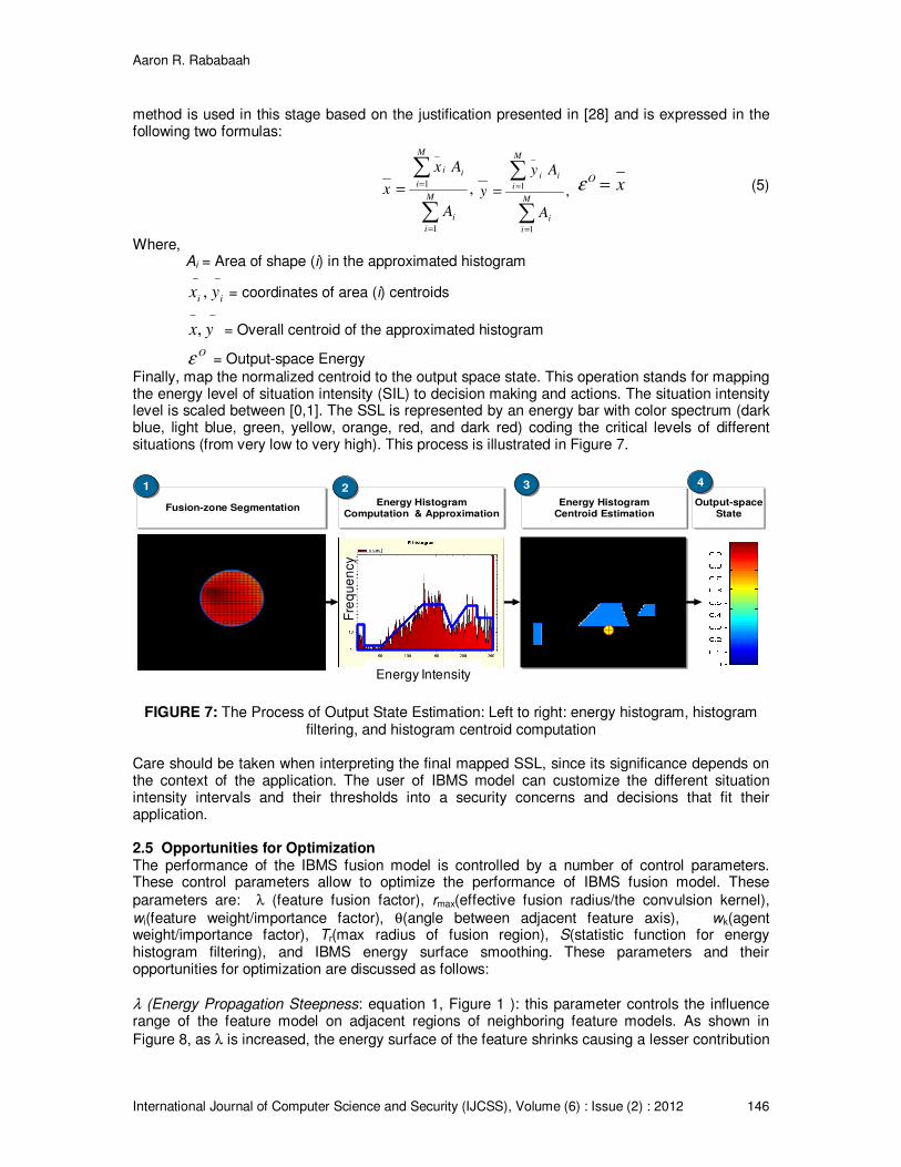
Finally, map the normalized centroid to the output space state. This operation stands for mapping the energy level of situation intensity (SIL) to decision making and actions. The situation intensity level is scaled between [0,1]. The SSL is represented by an energy bar with color spectrum (dark blue, light blue, green, yellow, orange, red, and dark red) coding the critical levels of different situations (from very low to very high). This process is illustrated in Figure 7.

Energy Histogram

Computation & Approximation

Energy HistogramComputation & Approximation

Energy Histogram

Centroid Estimation

Energy HistogramCentroid EstimationFusion-zone SegmentationFusion-zone Segmentation Output-space

State

Output-spaceState

11 22 33 44

Energy Intensity

Fre

qu

en

cy

FIGURE 7: The Process of Output State Estimation: Left to right: energy histogram, histogram filtering, and histogram centroid computation

Care should be taken when interpreting the final mapped SSL, since its significance depends on the context of the application. The user of IBMS model can customize the different situation intensity intervals and their thresholds into a security concerns and decisions that fit their application. 2.5 Opportunities for Optimization The performance of the IBMS fusion model is controlled by a number of control parameters. These control parameters allow to optimize the performance of IBMS fusion model. These

parameters are: λ (feature fusion factor), rmax(effective fusion radius/the convulsion kernel),

wi(feature weight/importance factor), θ(angle between adjacent feature axis), wk(agent weight/importance factor), Tr(max radius of fusion region), S(statistic function for energy histogram filtering), and IBMS energy surface smoothing. These parameters and their opportunities for optimization are discussed as follows:

λ (Energy Propagation Steepness: equation 1, Figure 1 ): this parameter controls the influence range of the feature model on adjacent regions of neighboring feature models. As shown in

Figure 8, as λ is increased, the energy surface of the feature shrinks causing a lesser contribution

Aaron R. Rababaah


to the fused energy surface. On the other hand, as λ decreases, the energy surface of the feature expands outwardly causing more interaction and contribution to the fused energy surface.

Therefore, an optimal setting of λ need to be found where the contributions and interactions of features can be optimized to meet the best output space state estimation

λ

)(tE

)(tε

1.0

0.0

λ

)(tE

)(tε

1.0

0.0

FIGURE 8: Effects of Feature Fusion Factor λ: Explains the influence range of feature energy on

the adjacent features. The arrow shows the increasing direction of λ

Effective Fusion Radius (rmax in Figure 3): this parameter controls the efficiency of the IBMS fusion algorithm. Without this parameter, the convolution algorithm needs to keep checking on reaching a minimal threshold value to terminate the convolution process. Therefore, solving this problem by introducing a kernel size that is the size of the effective fusion radius rmax makes the algorithm more efficient. Feature Weight (Importance Factor) (wi in Figure 4): this parameter can signifies the confidence in the current estimation of a particular feature. The higher this factor is, the more contribution and influence the associated feature to this factor should be given, and vice versa. The way this is modeled in IBMS is to let the energy model of the feature slide in and out toward and away from the fusion center causing the effect of the feature on the fused energy surface dynamically changing with respect to its wi. This phenomenon can be observed in Figure 9 Where, the weights of two features are kept unchanged, while the third one was assigned a higher wi value. The difference between the two maps is seen to be significant, as the energy surface toward the fusion center is elevated much more in the second (right) map than one in the first (left).

FIGURE 9: Effect of Feature Confidence Level on the Fused Energy Surface: Left: three feature each of which has a wi of (0.25). Right: two features remained with the same wi, while the third

feature was assigned a wi of (0.5)

Feature Alignment Angle (θi, in Figure 4): this parameter is used to populate and align the feature energy models on the energy map. This may have little or no effect on the fused energy surface. That is due to the fact that rotating a feature model around the fusion center will not increase or decrease its influence on the fused energy surface, it only affects the neighboring energy areas.

Aaron R. Rababaah


Whereas, as shown in the confidence level of features, sliding the energy model radially inward or outward drastically effect the IBMS fusion process. Figure 10 illustrates the impact of this parameter. In the first (left) map, one feature was rotated 45 degrees CW, where as in the second (right) map the same feature was slid toward the fusion center. The difference between the two maps is very clear, where the energy distribution in the second map was significantly altered compared to the first one.

FIGURE 10: Effect of Feature Weight VS. Feature Alignment Angle: Left: one feature is rotated 45 degrees CW. Right: same feature in left is slid toward the center.

Max Radius of Fusion Region: this parameter is very important to the optimization of IBMS, since it determines the most important region of the fused energy surface. Expanding and shrinking the fusion radius can drastically change the resulting energy histogram, from which the output state is inferred using the histogram centroid as presented earlier. The effect of this parameter is demonstrated in Figure 11. In Figure 11 all parameters kept static, but the radius of fusion circle was varied once (top) at 0.2 and a second time (bottom) at 0.9 of the map size. The resulting energy histograms differed drastically as expected. That is because, varying (limiting or expanding) the cropped fusion region will produce a different energy histogram and consequently a different estimation of the output state, which in this case changed from 0.7 to 0.4 with respect to 0.2 and 0.9 fusion radius respectively.

Energy Histogram

Energy Intensity

En

erg

y In

ten

sity

Energy Histogram

Energy Intensity

En

erg

y In

ten

sity

Aaron R. Rababaah


FIGURE 11: Fusion Radius Effects of the Energy Histogram: Top: fusion radius is set at 0.2 of the map. Bottom: fusion radius is set at 0.9 of the map.

Energy Histogram Filtering: one of the most efficient ways of histogram filtering is by down-sampling it. This method not only filters the histogram in the mean sense, but also reduces the dimensionality of the histogram which makes the subsequent step in IBMS fusion process more efficient, that is the Histogram Centroid Estimation. The question becomes what is the optimal size of the histogram and what statistic to use in filtering the adjacent bins: mean, median, or accumulation. To demonstrate the effects of down-sampling on the energy histogram, Figure 12 shows two histograms for the same cropped fusion region.

Energy Intensity

Fre

qu

en

cy

Energy Intensity

Fre

qu

en

cy

Energy Histogram Energy Histogram

FIGURE 12: Energy Histogram Down-Sampling and Filtering: Left: Energy histogram taken at 256 bins. Middle: the energy map for which the two histograms were computed. Right: Energy

histogram taken at 32 bins

As it can be observed in Figure 12, the down sampling of the energy histogram significantly smoothes the histogram but with the cost of shift it by 16% of the original value of the centroid of the histogram. For this reason an optimal size of the histogram need to be investigated.Energy Surface Smoothing: the results of the convolution operation in the IBMS fusion process can result in a noisy energy surface and needs to be smoothed. Using typical image processing filtering techniques including: mean, median, Gaussian filters, the surface can be integrated and smoothed out. To demonstrate this operation, Figure 13 illustrates the usage of a mean filter to smooth the energy surface.

FIGURE 13: Surface Energy Smoothing Using Image Mean Filtering: Left: Raw IBMS image. Right: smoothed IBMS image

SSL Profile Filtering: as it is anticipated with any model to have some level of noise interference due to causes including: sensor noise, feature estimation errors, feature energy noise interferences, etc. IBMS handles the noisy output state estimation by using Gaussian-based zero-phase (GZ) signal filter [29]. The GZ filter is temporally applied on the energy level resulting from

the equation (5) that is the output space energy (εo) as follows: let the filtered out space energy

be εo’, GZ be the Gaussian zero-phase filter then, ε

o’ can be expressed as follows:

Aaron R. Rababaah


),)(()('

ttGZtoo

∆±= εε (6)

Where,

∆t: the time interval (± ∆t) which the GZ is applied as in Figure 14.

In Figure 15, a demonstration of the GZ filter is depicted. The concept of GZ filter is to account for an interval of time before and after a particular sample point in a signal. In Figure 14, this sample

point is taken as sample number 5 and the time interval is ±3 units. Therefore the Gaussian PDF is superimposed on that interval aligning its mid-point with the sample point to be filtered. After

that, εo’

is computed as a linear combination of all contributions of each data point within the interval (5±3 units) in the example of Figure 14 according to the formula below:

∑∆+

∆−

=∆

tt

tt

o

pdf

o ttGttGZ )()(),)(( εε (7)

Figure 15 shows an example of applying the GZ filter on a simulated SSL signal, where it can be seen that it was very effective to eliminate noises significantly.

1 2 3 4 5 6 7 8 9 100

0.1

0.2

0.3

0.4

0.5

0.6

0.7

0.8

0.9

1

-1σ +1σ

-2σ-3σ +2σ +3σ

0σ

SSL

εεεεE

εεεεE’

Time1 2 3 4 5 6 7 8 9 10

0

0.1

0.2

0.3

0.4

0.5

0.6

0.7

0.8

0.9

1

-1σ +1σ

-2σ-3σ +2σ +3σ

0σ

SSL

εεεεE

εεεεE’

Time

FIGURE 14: Demonstration of Gaussian-based Signal Filtering

Aaron R. Rababaah


0 20 40 60 80 100 120 1400.45

0.5

0.55

0.6

0.65

0.7

0.75

Time

SSL

Raw SSL Tracking Filtered SSL Tracking

0 20 40 60 80 100 120 1400.45

0.5

0.55

0.6

0.65

0.7

0.75

Time

SSL

0 20 40 60 80 100 120 1400.45

0.5

0.55

0.6

0.65

0.7

0.75

Time

SSL

Raw SSL Tracking Filtered SSL Tracking

FIGURE 15: Demonstration of GZ Filter on a simulated SSL signal

2.6 Time Complexity Analysis Time complexity of an algorithm is defined as the mathematical function that asymptotically quantifies the growth of the computational time of the algorithm as a function of the size of the input. Typically, the time complexity is denoted as T(n) where, n is the size of the input. The asymptotic mathematical notations for T(n) of three types: O “big O” describes the upper bound of

an algorithm similar to “≤”, Ω “big omega” describes the lower bound of an algorithm, similar to “≥”

and Θ “big theta” describes the situation where, lower and upper bounds are the same function, similar to “=”. It is very critical for any model to stand the test of time complexity due to its direct impact on design efficiency, resources allocation, process throughput and response time. Therefore, it was top priority to conduct this time complexity analysis to investigate how our proposed model stands against a well-established soft-computing model, the Fuzzy Logic model. This section will present the analysis of the time complexity of the proposed model IBMS and will be compared to a fuzzy logic fusion model. The analysis will be conducted theoretically as well experimentally. Let n signify number of fuzzy inputs; m signify number of membership functions in a fuzzy input and m is assumed to be uniform across the n inputs to simplify the analysis. Then, it can be observed that a typical fuzzy model consists of four main stages: (1) Fuzzification, which is mapping operation of the crisp inputs into their fuzzy membership functions. This operation takes constant time per each input, therefore, its time complexity is O(1), hence for n inputs, the time complexity becomes O(n) as shown in the Figure 16. (2) Inference, which is applying the fuzzy rules onto the fuzzified inputs. This stage depends on the number of rules in the inference engine. The worst case scenario for such an inference system is to have as many as m

n number

of rules which is the inclusive case that cover all possible combinations of inputs to generate the rules for the engine, hence the time complexity of this stage is O(m

n). (3) Aggregation, which also

is bounded by the time complexity of the Inference stage, therefore, its time complexity is also O(m

n). (4) Defuzzification is the final stage in fuzzy logic system and it only operates on one

input, that is the aggregated areas of the membership functions to find the centroid of these combined areas, therefore it takes O(1) time. Finally, the total theoretical time needed for the fuzzy model to perform its fusion job in the worst case scenario is given by:

)1()()()( OmOmOnOnn

+++ (8)

Which in turn reduces to O(mn) since it is by far the greatest time complexity among all terms in

(8).

Aaron R. Rababaah


Fuzzification

Inference

Rule 1 w1

Rule 2 w2

Rule n wn

DefuzzificationAggregationCrisp

outputs

Crisp

inputs

)(n

mO

)(nO )(n

mO )1(O

Figure 16: Fuzzy Logic Time Complexity Theoretical Analysis. n = Number of inputs, m = Number of MFs. The red box signifies the dominant term in time complexity

IBMS consists also of four main stages (Figure 17): (1) Multi-feature fusion, which operates on n inputs and takes a constant time per feature, therefore, its time complexity is O(n). (2) Energy Histogram Computation and Approximation, which operates on the resulting fused image and it takes a constant time per fusion cycle, therefore, its time complexity is O(1). (3) Centroid Estimation, which operates on the resulting histogram from the preceding stage and it takes a constant time per fusion cycle, hence, it is time complexity is O(1). (4) Centroid to Energy Scale Mapping, which operates on the resulting centroid in the preceding stage and it takes a constant time every fusion cycle, therefore, its time complexity is O(1). Finally, the total theoretical time needed to perform a IBMS cycle can be expressed in (9) as:

)(nO )1(O )1(O )1(O

1wiθ

1Feature

2Feature

3Feature

4Feature nFeature

Input

Features

Feature Modeling

& Mapping

IBMS Fusion

None-linear Conv.Energy Histogram

Output State

Estimation

Decision

Space

FIGURE 17: IBMS Time Complexity Theoretical Analysis. n = Number of inputs. The red box signifies the dominant term in time complexity

)1()1()1()( OOOnO +++ (9)

Which reduces to O(n) which is by far the greatest term in equation 9. Comparing the two results of fuzzy time complexity “O(m

n)” and IBMS time complexity “O(n)”, theoretically, reveals that the

IBMS model has a linear time complexity, whereas, the fuzzy model has an exponential time complexity. The Fuzzy logic model has significantly greater time complexity as can be expressed in the following asymptotic notation:

0)(

)(=

∞→

nn mO

nOLim (10)

Which states that as n grows to huge values, IBMS time complexity compared to that of fuzzy logic is negligible. To support this theoretical finding, a set of experiments were conducted on both models to test their time responses by varying number of input features to the models between [1 to 10] and observe their responses. These experiments are summarized Table 1 and Figure 18 respectively.

Aaron R. Rababaah


Table 1 and its graphical plotting in Figure 18 clearly proves that the fuzzy model time complexity follows an exponential curve while the IBMS time complexity follows a linear response.

TABLE 1: Experimental Time Responses Measured for IBMS vs. FUZZY

FIS FEAM FEAM/FIS

2 10.48 31.25 2.98

3 16.17 46.88 2.90

4 22.83 57.81 2.53

5 31.85 62.50 1.96

6 46.61 75.00 1.61

7 75.26 81.00 1.08

8 137.56 87.50 0.64

9 281.44 96.88 0.34

10 622.99 104.69 0.17

Time Responces (ms)Number of

Features Fuzzy IBMS IBMS/Fuzzy

2 3 4 5 6 7 8 9 100

100

200

300

400

500

600

700

Number of Input Features

Response T

ime

Fuzzy Fusion Model

FEAM-FE Model

Linear Growth

Power Growth

IBMS Fusion Model

Fuzzy Fusion Model

)(nO

)(nmO

FIGURE 18: Time Response Performance of IBMS Vs. Fuzzy

3. CONCLUSIONS AND FUTURE WORK We have presented a new an image-based fusion model for multi-sensor multi-source data fusion (IBMS). A complete and detailed theoretical development and analysis was presented for the fusion process of the proposed model. IBMS demonstrated reliability and efficiency over fuzzy logic model. It was found to be superior in time complexity both theoretically and experimentally. As a fusion engine, IBMS has potentials in data and information fusion in areas where the concept of IBMS is applicable. The concept of IBMS is based on the principles of the multi sensor

Aaron R. Rababaah


data fusion [16], where multiple sources can have different views of the same situation without necessarily the same feature directionality. This situation entails a method to combine these sources of information to come up with a unified view of the events in a particular environment and enhance the situation awareness. Potential applications of IBMS include: Application in General Surveillance Systems - The IBMS energy map dynamically changes upon the discovery of changes in any of the mapped features and the whole process of IBMS fusion accordingly responds to these changes as it was demonstrated earlier as more evidence about SSL (depending on the context of the application) IBMS intensifies its fusion surface and accordingly the SSL is elevated so a corresponding decision can be taken. In the light of this concept, some potential application include: military sites surveillance, government facility surveillance systems, boarder security, university campus security systems, law informant surveillance for public area monitoring, etc. Application of IBMS in the Fusion Process - Another potential application of the IBMS model is supporting the JDL fusion model. To relate IBMS to the JDL model, it can be observed that this concept is related to level 2 processing (situation assessment) in the MSDF process of JD. As for the hierarchy of data fusion inference the proposed model of fits two levels of inference: object behavior and situation assessment. This is due to the fact that the proposed model in this work addresses target/phenomena characterization using multi-modality framework for EOI inference and situation assessment. Application of IBMS in Resource Allocation Optimization - Optimization of resources in fusion models (JDL level-4) is very essential and vital for survival and management of the available resources. Mapping available resources to situation requirements is a complex task and needs dynamic intelligent techniques and models to approach it. IBMS model can be utilized to generate the situation map by projecting foe events on the energy map and try to allocate the resources maps to better allocate what resource(s) to what location(s) and events currently occurring in spatial and temporal space of IBMS model.

4. REFERENCES [01] Trivedi Mohan M., Gandhi Tarak L., and Huang Kohsia S., “Distributed Interactive. Video

Arrays for Event Capture and Enhanced Situational Awareness,” in the 2005 IEEE Intelligent Systems.

[02] Koller D., Weber J., Huang T., Malik J., Ogasawara G., Rao B., and Russell S., “ Toward Robust Automatic Traffic Scene Analysis in Real-Time,” IEEE Computer Science Division University of California, Berkeley, CA, 1994. http://dx.doi.org/10.1109/ICPR.1994.576243

[03] Kogut Greg, Blackburn Mike, Everett H.R., “Using Video Sensor Networks to Command and Control Unmanned Ground Vehicles,” Space and Naval Warfare Systems Center San Diego, 2000. www.spawar.navy.mil/robots/pubs/usis03diva.pdf

[04] Chang Edward Y. and Wang Yuan-Fang, “Toward Building a Robust and Intelligent Video Surveillance System: A Case Study,” Dept. of Electrical and Computer Engineering Dept. of Computer Science, Univ. of California, 2003. www.cs.ucsb.edu/~yfwang/papers/icme04_invited.pdf

[05] Bodo Robert, Jackso Bennett, and Papanikolopoulos Nikolaos, “Vision-Based Human Tracking and Activity Recognition,” 2002. AIRVL, Dept. of Computer Science and Engineering, University of Minnesota. http://mha.cs.umn.edu/Papers/Vision_Tracking_Recognition.pdf

[07] Ma Yunqian, Miller Ben, Buddharaju Pradeep, Bazakos Mike, “Activity Awareness: From Predefined Events to New Pattern Discovery,” Proceedings of the Fourth IEEE International Conference on Computer Vision Systems (ICVS 2006). www.cs.colostate.edu/icvs06/Program.pdf

Aaron R. Rababaah


[08] Collins Robert T., Lipton Alan J., Fujiyoshi Hironobu and Fellow Takeo Nade, IEEE, “Algorithms for Cooperative Multi-sensor Surveillance,” 2001. Processing of the IEEE, VOL. 89, NO. 10, October 2001.

[09] Goh King-Shy, Miyahara Koji, Radhakrishan Regunathan, Xiong Ziyou, and Divakaran Ajay, Audio-Visual Event Detection based on Mining of Semantic Audio-Visual Labels, MERL – A MITSUBISHI ELECTRIC RESEARCH LABORATORY, http://www.merl.comTR-2004-008 March 2004

[10] Varshney Pramod K., Mehrotra Kishan G., and Mohan Chilukuri K., Decision Making and Reasoning with Uncertain Image and Sensor Data, Syracuse University. http://www-video.eecs.berkeley.edu/vismuri/meeting2006/syracuse.ppt

[11] Klapuri, Audio signal classification, ISMIR Graduate School, October 4th-9th, 2004, http://mtg.upf.edu/ismir2004/graduateschool/people/Klapuri/classification.pdf

[12] Temko Andrey, Malkin Robert, Zieger Christian, Macho Dusan, Nadeu Climent, and Omologo Maurizio, Acoustic Event Detection And Classification In Smart-Room Environments: Evaluation Of Chil Project Systems, TALP Research Center, UPC, Barcelona, Spain, interACT, CMU, Pittsburgh, USA, ITC-irst, Povo (TN), Italy Zaragoza • Del 8 al 10 de Noviembre de 2006.

[13] Stauffer Chris, Automated Audio-visual Activity Analysis, Compute Science and Artificial Intelligence Laboratory, MIT-CAAIL-TR-2005-057, AIM-2005-026, 09, 20, 2005

[14] Chen Datong, Malkin Robert, Yang Jie, Multimodal Detection of Human Interaction Events in a Nursing Home Environment, School of Computer Science, Carnegie Mellon University, Sixth International Conference on Multimodal Interfaces (ICMI'04), Penn State University, State College, PA, October 14-15, 2004

[15] Gerosa L., Valenzise G., Tagliasacchi M., Antonacci F., and Sarti A.. Scream And Gunshot Detection In Noisy Environments, Dipartimento di Elettronica e Informazione, Politecnico di Milano, Italy, VISNET II, a network of excellence 2006.

[16] Hall David L. and McMullen Sonya A. H. Mathematical Techniques in Multisensor Data Fusion, 2nd edition, 2004. Artech House, INC. Norwood, MA.

[17] Brooks Alex and Williams Stefan, “Tracking People with Networks of Heterogeneous Sensors,” ARC Centre of Excellence in Autonomous Systems. School of Aerospace, Mechanical, and Mechatronic Engineering, University of Sydney, NSW Australia, 2003 www.acfr.usyd.edu.au/publications/downloads/2004/Brooks210/Brooks03Tracking.pdf

[18] Meyer Michael, Ohmacht Thorsten and Bosch Robert GmbH and Michael Hotter, “Video Surveillance Applications Using Multiple Views of a Scene,” IEEE AES Systems Magazine, March 1999.

[19] Turollu A., Marchesotti L. and Regazzoni C.S., “Multicamera Object Tracking In Video Surveillance Applications,” DIBE, University of Genoa, Italy, 2001. http://cmp.felk.cvut.cz/cvww2006/papers/39/39.pdf

[20] Niu Wei, Long Jiao, Han Dan, and Wang Yuan-Fang, “Human Activity Detection and Recognition for Video Surveillance,” the 2004 IEEE International Conference on Multimedia and Expo. www.cs.ucsb.edu/~yfwang/papers/icme04_tracking.pdf

Aaron R. Rababaah


[21] Siebel Nils T. and Maybank Steve, “Fusion of Multiple Tracking Algorithms for Robust People Tracking, Annotated Digital Video for Intelligent Surveillance and Optimized Retrieval (ADVISOR),”. Computational Vision Group, Department of Computer Science, The University of Reading, Reading RG6 6AY, England, 2001. www.cvg.reading.ac.uk/papers/advisor/ECCV2002.pdf

[22] Ellis Tim. Multi-camera Video Surveillance. 2002. Information Engineering Center, School of engineering, City university, London. 0-7803-7436-3/02 2002 IEEE.

[23] Snidaro L., Niu R., Varshney P.K., and Foresti G.L., “Automatic Camera Selection and Fusion for Outdoor Surveillance Under Changing Weather Conditions,” Dept. of Mathematics and Computer Science, University of Udine, Ital, Department of EECS, Syracuse University, NY, 2003. www.ecs.syr.edu/research/SensorFusionLab/Downloads/Rrixin%20Niu/avss03.pdf

[24] Boult Terrance E., “Geo-spatial Active Visual Surveillance on Wireless Networks,” Proceedings of the 32nd Applied Imagery Pattern Recognition Workshop. http://vast.uccs.edu/.../PAPERS/IEEE-IAPR03-Geo-Spatial_active_Visual_Surveillance-On-Wireless-Networks-Boult.pdf

[25] Chang Edward Y. and Wang Yuan-Fang, “Toward Building a Robust and Intelligent Video Surveillance System: A Case Study,” Dept. of Electrical and Computer Engineering Dept. of Computer Science, Univ. of California, 2003. www.cs.ucsb.edu/~yfwang/papers/icme04_invited.pdf

[26] A. Turolla, L. Marchesotti and C.S. Regazzoni, “Multicamera Object Tracking in Video Surveillance Applications”, DIBE, University of Genoa, Italy

[27] Sensory Physiology Lettuces at University Minnesota Dulutth, 03.17.2012. http://www.d.umn.edu/~jfitzake/Lectures/DMED/SensoryPhysiology/GeneralPrinciples/CodingTheories.html

[28] MatLab Documentation on Fuzzy Logic. MatLab7 R14. The MathWorks Documentation. http://www.mathworks.com/access/helpdesk/help/toolbox/fuzzy/fuzzy.html?BB=1

[29] MatLab Documentation on Signal Processing – Signal Windowing models. MatLab7 R14. The MathWorks Documentation. http://www.mathworks.com/documentation/signalprocessing/hamming

image-based multi-sensor data representation and fusion via 2d non-linear convolution

Education