ILC Beam Dynamics Studies

Using PLACET

Andrea Latina (CERN)

July 11, 2007

John Adams Institute for Accelerator Science - Oxford (UK)

• Introduction

• Simulations Results

• Conclusions and Outlook

PLACET Physical Highlights

• PLACET is a tracking code that simulates beam transport and orbit correction in linearcolliders

• it implements synchrotron radiation emission

• it takes into account collective effects such as:

- short/long range wakefieldsin the accelerating structuresin the crab cavities,

- multi-bunch effects and beam loading,

- geometric and resistive wall wakes in the collimators

• it can track the longitudinal phase space

• it can track sliced beams as well as beams of single particles, and can switch betweenthem during tracking

⇒ It can simulate: bunch compressor, main linac, drive beam, beam delivery system (includingcrab cavities and instrumentation), interaction point (using Guinea-Pig) and soon : postcollision line

PLACET Technical Highlights

• It is -relatively- easy to use

• It is fully programmable and modular, thanks to its Tcl/Tk interface and its externalmodules:

- it allows the simulation of feedback loops

- ground motion effects are easy to include

- external MPI parallel tracking module (limited tracking)

• It is open to other codes:

- it can read MAD/MAD-X deck files, as well as XSIF files

- can be easily interfaced to Guinea-Pig

- it can use other codes to perform beam transport

• It has a graphical interface

• [NEW] it embeds Octave, a mathematical toolbox like MatLab (but free)

- rich set of numerical tools

- easy to use optimization / control system tool-boxes

Emittance Preservation and ILPS

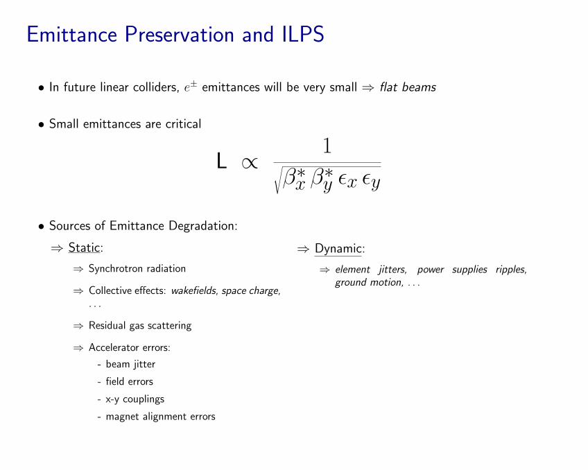
• In future linear colliders, e± emittances will be very small ⇒ flat beams

• Small emittances are critical

L ∝ 1√β∗x β∗y εx εy

• Sources of Emittance Degradation:

⇒ Static:

⇒ Synchrotron radiation

⇒ Collective effects: wakefields, space charge,. . .

⇒ Residual gas scattering

⇒ Accelerator errors:

- beam jitter

- field errors

- x-y couplings

- magnet alignment errors

⇒ Dynamic:

⇒ element jitters, power supplies ripples,ground motion, . . .

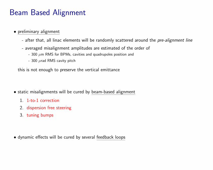
Beam Based Alignment

• preliminary alignment

- after that, all linac elements will be randomly scattered around the pre-alignment line

- averaged misalignment amplitudes are estimated of the order of- 300 µm RMS for BPMs, cavities and quadrupoles position and

- 300 µrad RMS cavity pitch

this is not enough to preserve the vertical emittance

• static misalignments will be cured by beam-based alignment

1. 1-to-1 correction

2. dispersion free steering

3. tuning bumps

• dynamic effects will be cured by several feedback loops

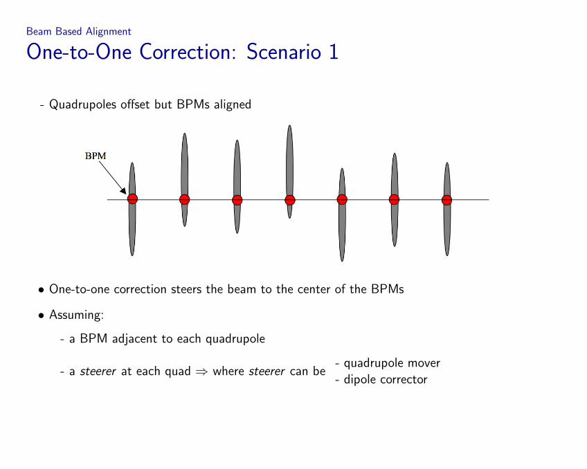
Beam Based Alignment

One-to-One Correction: Scenario 1

- Quadrupoles offset but BPMs aligned

• One-to-one correction steers the beam to the center of the BPMs

• Assuming:

- a BPM adjacent to each quadrupole

- a steerer at each quad ⇒ where steerer can be- quadrupole mover- dipole corrector

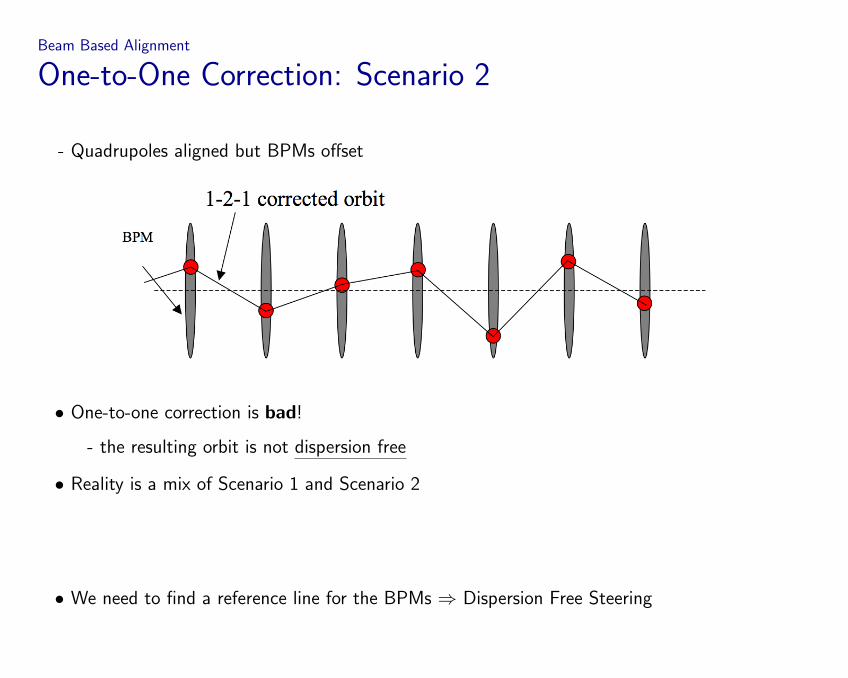
Beam Based Alignment

One-to-One Correction: Scenario 2

- Quadrupoles aligned but BPMs offset

• One-to-one correction is bad!

- the resulting orbit is not dispersion free

• Reality is a mix of Scenario 1 and Scenario 2

• We need to find a reference line for the BPMs ⇒ Dispersion Free Steering

Beam Based Alignment

Dispersion Free Steering

DFS attempts to correct dispersion and trajectory at the same time

⇒ A nominal beam + one or more test beams with different energies are used to determine thedispersion along the linac.

⇒ The nominal trajectory is steered and the differences between the nominal and the off-energy

trajectories are minimized:

χ2 =n∑

i=1y2

0,i +m∑

j=1

n∑i=1

ω1,j (yj,i − y0,i −∆i)2 +

p∑k=1

ω2,k c2k

i = 1..n BPMsj = 0..m beams (j = 0, nominal beam)k = 1..p correctorsω1,i, ω2,j weights for dispersion and correction terms

yi,j position of beam j in BPM i∆i target dispersion at BPM ick strength for the corrector k

• The beamline is divided into bins of BPMs and correctors

• We propose to use the Bunch Compressor to generate the test beams

Recent Simulation Results

• Bunch Compressor (BC)

- Alignment

• Main Linac (ML)

- Static alignment strategies for a laser-straight and a curved layout

- use of BC to align the ML

- impact of BPM calibration errors and quadrupole power supply ripples

- Dynamic Effects

- jitter during alignment

- orbit feedback to cure ground motion

• Beam Delivery System (BDS)

- Feedback Studies

- Crab Cavity Simulation

- Collimator Wakefields and Halo Particles

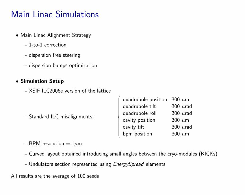
Main Linac Simulations

• Main Linac Alignment Strategy

- 1-to-1 correction

- dispersion free steering

- dispersion bumps optimization

• Simulation Setup

- XSIF ILC2006e version of the lattice

- Standard ILC misalignments:

quadrupole position 300 µmquadrupole tilt 300 µradquadrupole roll 300 µradcavity position 300 µmcavity tilt 300 µradbpm position 300 µm

- BPM resolution = 1µm

- Curved layout obtained introducing small angles between the cryo-modules (KICKs)

- Undulators section represented using EnergySpread elements

All results are the average of 100 seeds

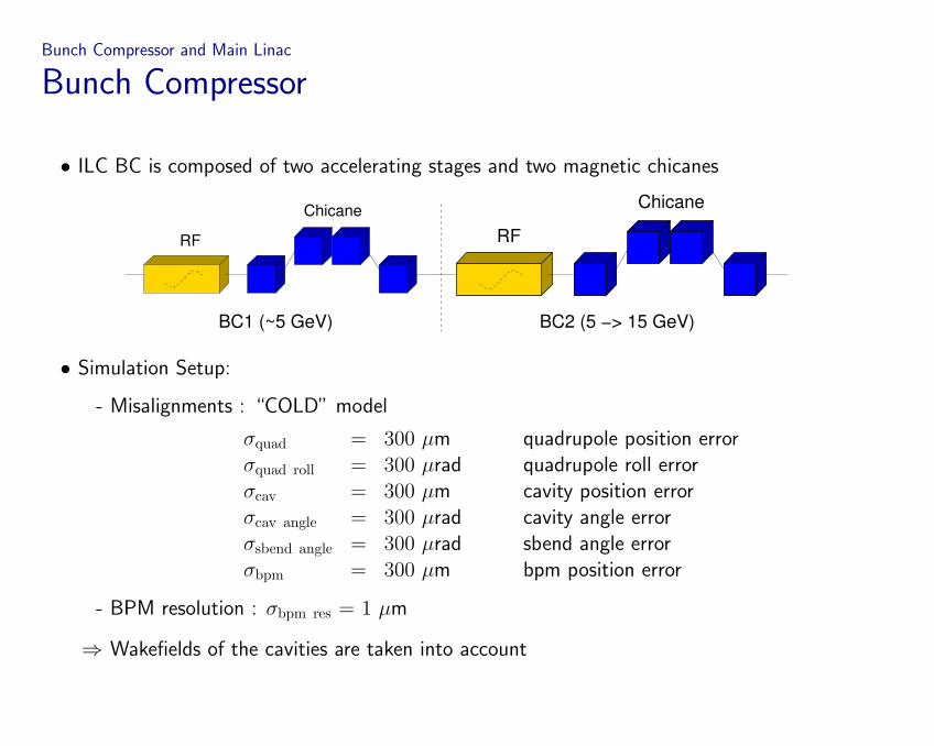
Bunch Compressor and Main Linac

Bunch Compressor

• ILC BC is composed of two accelerating stages and two magnetic chicanes

RF

Chicane

BC2 (5 −> 15 GeV)BC1 (~5 GeV)

RF

Chicane

• Simulation Setup:

- Misalignments : “COLD” model

σquad = 300 µm quadrupole position errorσquad roll = 300 µrad quadrupole roll errorσcav = 300 µm cavity position errorσcav angle = 300 µrad cavity angle errorσsbend angle = 300 µrad sbend angle errorσbpm = 300 µm bpm position error

- BPM resolution : σbpm res = 1 µm

⇒ Wakefields of the cavities are taken into account

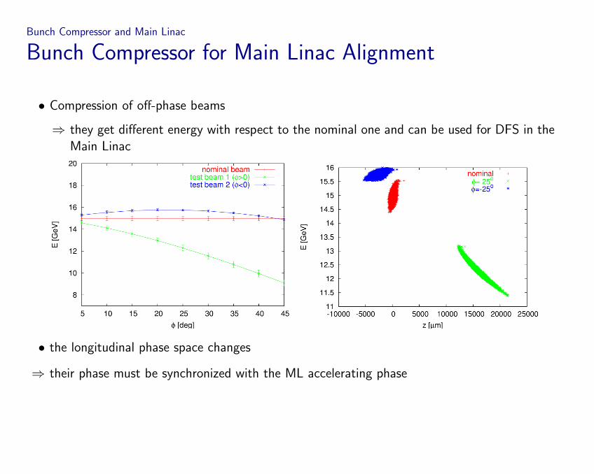
Bunch Compressor and Main Linac

Bunch Compressor for Main Linac Alignment

• Compression of off-phase beams

⇒ they get different energy with respect to the nominal one and can be used for DFS in theMain Linac

• the longitudinal phase space changes

⇒ their phase must be synchronized with the ML accelerating phase

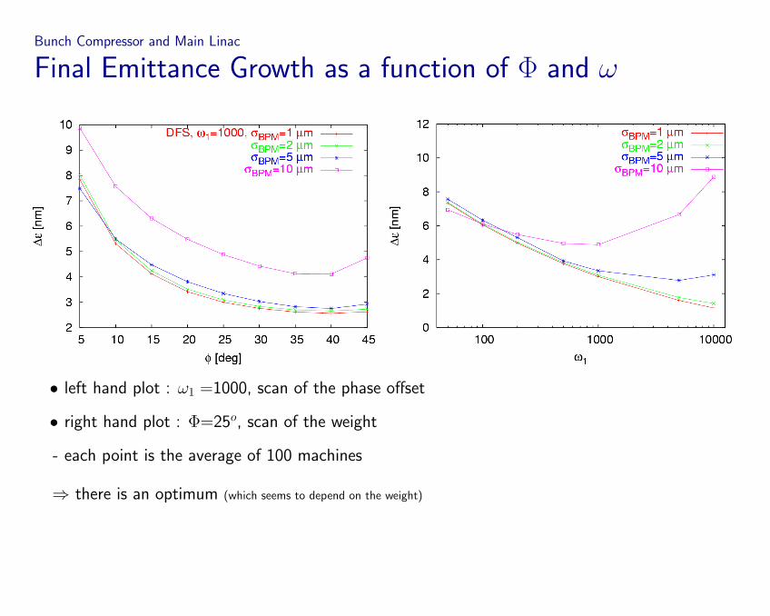
Bunch Compressor and Main Linac

Final Emittance Growth as a function of Φ and ω

• left hand plot : ω1 =1000, scan of the phase offset

• right hand plot : Φ=25o, scan of the weight

- each point is the average of 100 machines

⇒ there is an optimum (which seems to depend on the weight)

Main Linac

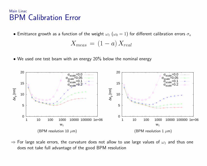
BPM Calibration Error

• Emittance growth as a function of the weight ω1 (ω0 = 1) for different calibration errors σa

Xmeas = (1− a) Xreal

• We used one test beam with an energy 20% below the nominal energy

0

5

10

15

20

1 10 100 1000 10000 100000 1e+06

∆εy

[nm

]

w1

σscale=0.0σscale=0.05

σscale=0.1σscale=0.2

0

5

10

15

20

1 10 100 1000 10000 100000 1e+06

∆εy

[nm

]

w1

σscale=0.0σscale=0.05

σscale=0.1σscale=0.2

(BPM resolution 10 µm) (BPM resolution 1 µm)

⇒ For large scale errors, the curvature does not allow to use large values of ω1 and thus onedoes not take full advantage of the good BPM resolution

Main Linac

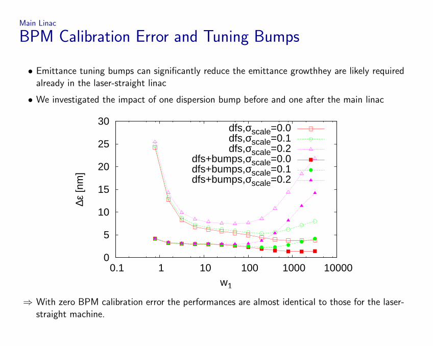
BPM Calibration Error and Tuning Bumps

• Emittance tuning bumps can significantly reduce the emittance growthhey are likely requiredalready in the laser-straight linac

• We investigated the impact of one dispersion bump before and one after the main linac

0

5

10

15

20

25

30

0.1 1 10 100 1000 10000

∆ε [n

m]

w1

dfs,σscale=0.0dfs,σscale=0.1dfs,σscale=0.2

dfs+bumps,σscale=0.0dfs+bumps,σscale=0.1dfs+bumps,σscale=0.2

⇒ With zero BPM calibration error the performances are almost identical to those for the laser-straight machine.

Bunch Compressor and Main Linac

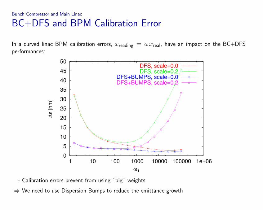
BC+DFS and BPM Calibration Error

In a curved linac BPM calibration errors, xreading = a xreal, have an impact on the BC+DFSperformances:

0

5

10

15

20

25

30

35

40

45

50

1 10 100 1000 10000 100000 1e+06

∆ε [n

m]

ω1

DFS, scale=0.0DFS, scale=0.2

DFS+BUMPS, scale=0.0DFS+BUMPS, scale=0.2

- Calibration errors prevent from using “big” weights

⇒ We need to use Dispersion Bumps to reduce the emittance growth

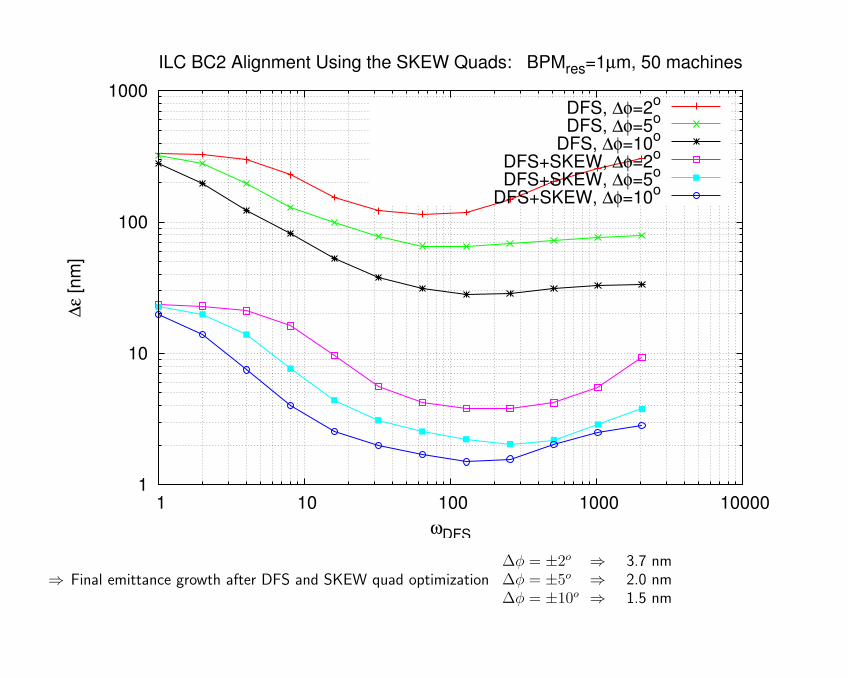
Bunch Compressor Alignment

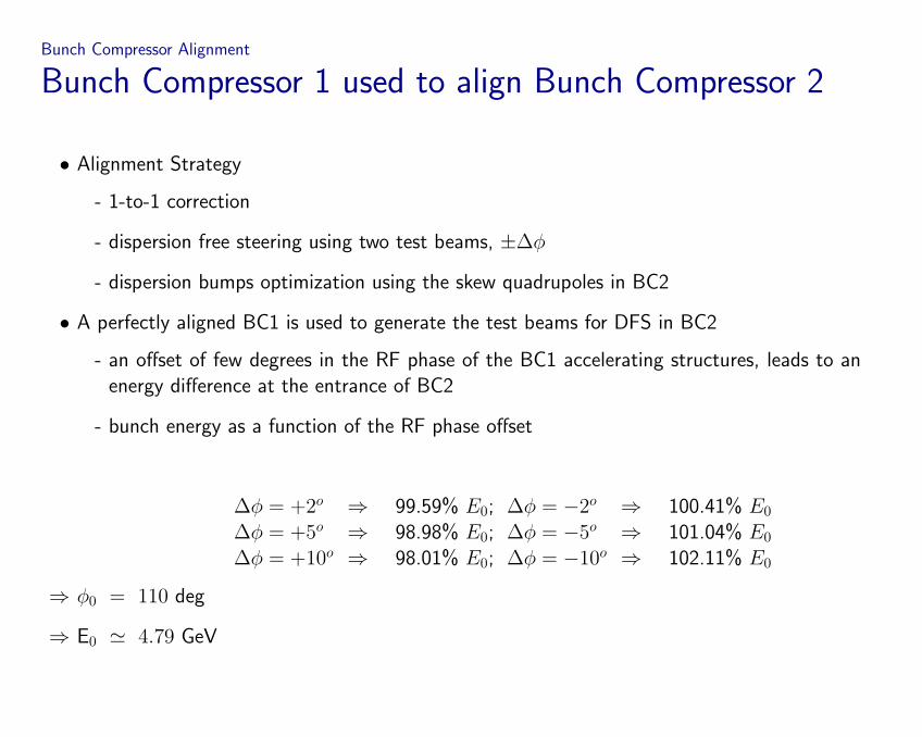
Bunch Compressor 1 used to align Bunch Compressor 2

• Alignment Strategy

- 1-to-1 correction

- dispersion free steering using two test beams, ±∆φ

- dispersion bumps optimization using the skew quadrupoles in BC2

• A perfectly aligned BC1 is used to generate the test beams for DFS in BC2

- an offset of few degrees in the RF phase of the BC1 accelerating structures, leads to anenergy difference at the entrance of BC2

- bunch energy as a function of the RF phase offset

∆φ = +2o ⇒ 99.59% E0;∆φ = +5o ⇒ 98.98% E0;∆φ = +10o ⇒ 98.01% E0;

∆φ = −2o ⇒ 100.41% E0

∆φ = −5o ⇒ 101.04% E0

∆φ = −10o ⇒ 102.11% E0

⇒ φ0 = 110 deg

⇒ E0 ' 4.79 GeV

1

10

100

1000

1 10 100 1000 10000

∆ε [n

m]

ωDFS

ILC BC2 Alignment Using the SKEW Quads: BPMres=1µm, 50 machines

DFS, ∆φ=2o

DFS, ∆φ=5o

DFS, ∆φ=10o

DFS+SKEW, ∆φ=2o

DFS+SKEW, ∆φ=5o

DFS+SKEW, ∆φ=10o

⇒ Final emittance growth after DFS and SKEW quad optimization∆φ = ±2o ⇒ 3.7 nm∆φ = ±5o ⇒ 2.0 nm∆φ = ±10o ⇒ 1.5 nm

0.01

0.1

1

10

100

1 10 100 1000 10000

∆ε [n

m]

ωDFS

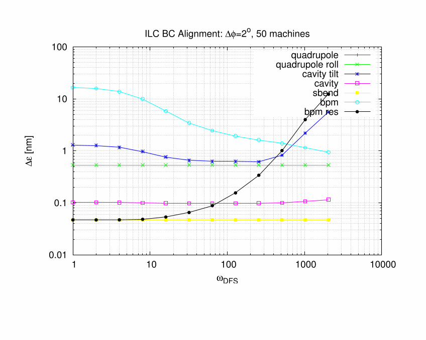
ILC BC Alignment: ∆φ=2o, 50 machines

quadrupolequadrupole roll

cavity tiltcavitysbend

bpmbpm res

Dynamic Effects in the Main Linac

Luminosity Loss Due to Quadrupole Jitter

Simulation parameters:

- we used GUINEA-PIG to calculate the luminosity

- a perfect machine has been used in the simulation

- and the end of the linac an intra-pulse feedback has been used to remove incoming beamposition and angle errors at a single point

- quadrupoles in the electron linac have been scattered, while the ones in the positron linac arekept fixed

- the beam delivery system is represented by a transfer matrix: the end-of-linac Twiss param-eters are transformed into the ones at the IP

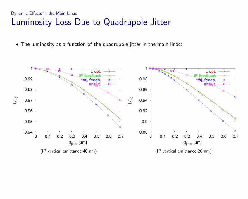
Dynamic Effects in the Main Linac

Luminosity Loss Due to Quadrupole Jitter

• The luminosity as a function of the quadrupole jitter in the main linac:

(IP vertical emittance 40 nm) (IP vertical emittance 20 nm)

Dynamic Effects in the Main Linac

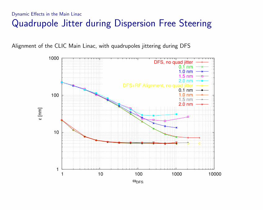
Quadrupole Jitter during Dispersion Free Steering

Alignment of the CLIC Main Linac, with quadrupoles jittering during DFS

1

10

100

1000

1 10 100 1000 10000

ε [n

m]

ωDFS

DFS, no quad jitter0.1 nm1.0 nm1.5 nm2.0 nm

DFS+RF Alignment, no quad jitter0.1 nm1.0 nm1.5 nm2.0 nm

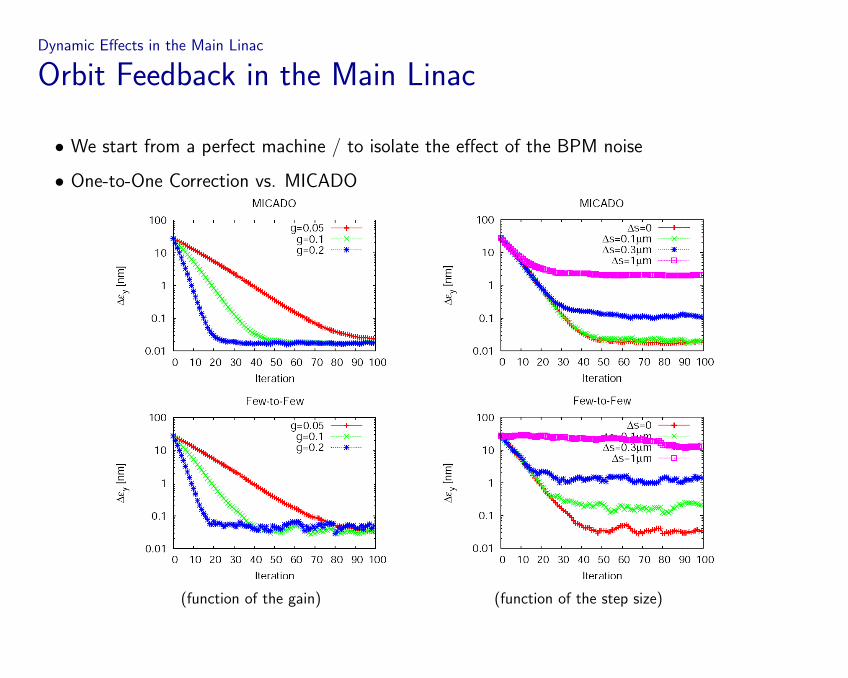
Dynamic Effects in the Main Linac

Orbit Feedback in the Main Linac

• We start from a perfect machine / to isolate the effect of the BPM noise

• One-to-One Correction vs. MICADO

(function of the gain) (function of the step size)

Beam Delivery System

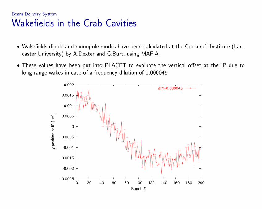
Wakefields in the Crab Cavities

• Wakefields dipole and monopole modes have been calculated at the Cockcroft Institute (Lan-caster University) by A.Dexter and G.Burt, using MAFIA

• These values have been put into PLACET to evaluate the vertical offset at the IP due tolong-range wakes in case of a frequency dilution of 1.000045

-0.0025

-0.002

-0.0015

-0.001

-0.0005

0

0.0005

0.001

0.0015

0.002

0 20 40 60 80 100 120 140 160 180 200

y po

sitio

n at

IP [m

m]

Bunch #

∆f/f=0.000045

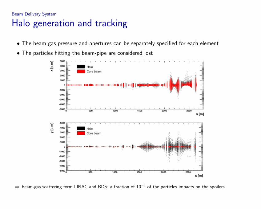
Beam Delivery System

Halo generation and tracking

• The beam gas pressure and apertures can be separately specified for each element

• The particles hitting the beam-pipe are considered lost

⇒ beam-gas scattering form LINAC and BDS: a fraction of 10−4 of the particles impacts on the spoilers

Beam Delivery System

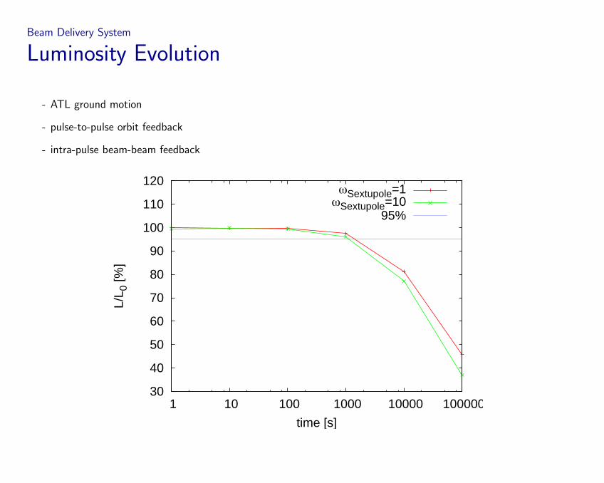
Luminosity Evolution

- ATL ground motion

- pulse-to-pulse orbit feedback

- intra-pulse beam-beam feedback

30

40

50

60

70

80

90

100

110

120

1 10 100 1000 10000 100000

L/L 0

[%]

time [s]

ωSextupole=1ωSextupole=10

95%

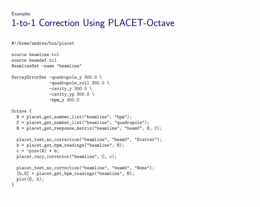
Examples

1-to-1 Correction Using PLACET-Octave

#!/home/andrea/bin/placet

source beamline.tcl

source beamdef.tcl

BeamlineSet -name "beamline"

SurveyErrorSet -quadrupole_y 300.0 \

-quadrupole_roll 300.0 \

-cavity_y 300.0 \

-cavity_yp 300.0 \

-bpm_y 300.0

Octave {

B = placet_get_number_list("beamline", "bpm");

C = placet_get_number_list("beamline", "quadrupole");

R = placet_get_response_matrix("beamline", "beam0", B, C);

placet_test_no_correction("beamline", "beam0", "Scatter");

b = placet_get_bpm_readings("beamline", B);

c = -pinv(R) * b;

placet_vary_corrector("beamline", C, c);

placet_test_no_correction("beamline", "beam0", "None");

[b,S] = placet_get_bpm_readings("beamline", B);

plot(S, b);

}

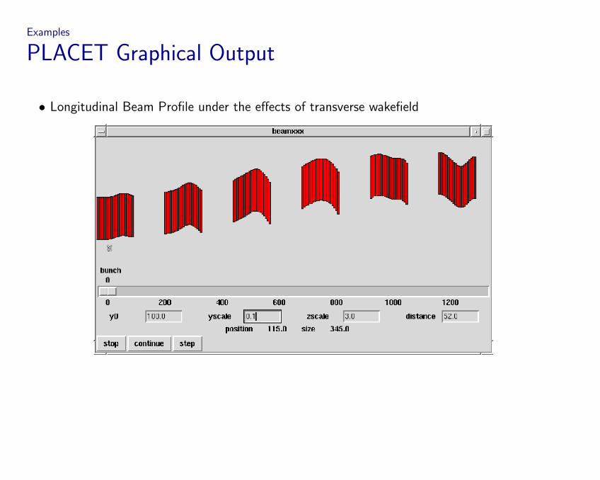
Examples

PLACET Graphical Output

• Longitudinal Beam Profile under the effects of transverse wakefield

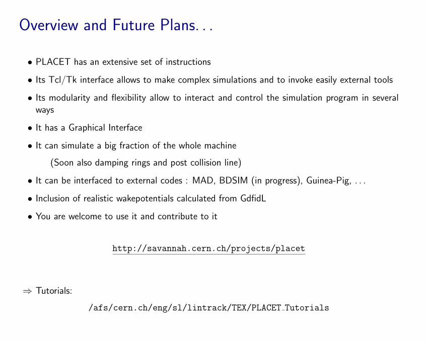
Overview and Future Plans. . .

• PLACET has an extensive set of instructions

• Its Tcl/Tk interface allows to make complex simulations and to invoke easily external tools

• Its modularity and flexibility allow to interact and control the simulation program in severalways

• It has a Graphical Interface

• It can simulate a big fraction of the whole machine

(Soon also damping rings and post collision line)

• It can be interfaced to external codes : MAD, BDSIM (in progress), Guinea-Pig, . . .

• Inclusion of realistic wakepotentials calculated from GdfidL

• You are welcome to use it and contribute to it

http://savannah.cern.ch/projects/placet

⇒ Tutorials:

/afs/cern.ch/eng/sl/lintrack/TEX/PLACET Tutorials