ii performance prediction for high speed craft anuar … · kapal dengan foil buritan atau...

ii

PERFORMANCE PREDICTION FOR HIGH SPEED CRAFT

ANUAR BIN BERO

A dissertation submitted in partial fulfillment of the

requirements for the award of the degree of

Master of Engineering (Marine Technology)

Faculty of Mechanical Engineering

Universiti Teknologi Malaysia

MAY 2009

iv

Dedicated with love to my wife and children

v

ACKNOWLEDGEMENT

In the name of ALLAH the most Merciful and praise to Prophet Muhamad

S.A.W, i am able to complete my thesis. I wish to express my sincere appreciation to

my thesis supervisor Ir. Dr. Mohamad Pauzi bin Abd Ghani for encouragement,

guidance, critics and friendship. Without his continued support and concern, this

thesis would not have been completed.

I also would like to express my gratitude to Researcher Officer and all

technicians at Marine Technology Laboratory, UTM for assisting me in conducting

model testing. I am also thankful to Librarians of Universiti Teknologi Malaysia

(PSZ UTM Skudai) for their assistance in providing the relevant literatures.

Furthermore, i want to express my appreciation to my Head of Engineering Faculty,

Cdr Mazlan Bin Yassin RMN for his support and motivation while completing this

thesis.

Special gratitude to my beloved wife Habsah and children Iman and Hazim

for their support and inspiration during my research study. Also thank to my mother,

father and to my colleague, your support will be remembered.

vi

ABSTRACT

Generally the performance of the high speed craft can be divided into six

main components such as resistance and powering, propulsion, dynamic instability,

seakeeping and manoeuvring. Performance prediction on high speed craft especially

in planing hull is complicated due to complex combination of ship behaviour in

rough sea condition. The performance of high speed craft is becoming more

important due to their various functions and purposes to marine community which is

unable to be predicted using conventional methods. The fundamental of this research

is to study the two main components of the vessel i.e. resistance and seakeeping

quality by incorporating stern foil at aft portion planing craft (M Hull) that gives

significant effect to the performance of the vessel. Theoretically, stern foil has a

similar function with transom flap, trim wedges and trim tab which is to reduce the

resistance and also as a damping for motion reduction. In the scope of resistance

performance for this vessel with stern foil, the Savitsky and two dimensional

Methods are used for resistance prediction at different angle of attack. While

Computational Methods i.e. SEAKEEPER program was applied to seakeeping

prediction in regular wave (head sea). Both result of resistance and seakeeping

performance prediction was validated by conducting model test for the model with

and without stern foil. The performance of ship model with stern foil gives a positive

performance in term of seakeeping quality at constructive resistance. By adapting

with stern foil the heave and pitch Response Amplitude Operator (RAO) trim down

by 4.0% and 18.91% respectively. Furthermore, the reduction of forward and aft

acceleration RAO also occurs concurrently which the decreasing of both acceleration

are 21.10% and 6.14%.

vii

ABSTRAK

Secara amnya, prestasi kapal laju dibahagikan kepada enam komponen utama

iaitu rintangan dan daya tujahan, dorongan, ketidakstabilan dinamik, seakeeping dan

manoeuvring. Anggaran terhadap prestasi kapal laju terutamanya planing hull adalah

sangat sukar disebabkan gandingan sifat kapal yang komplek pada keadaan laut yang

bergelora. Kajian ini lebih menumpukan kepada dua perkara iaitu rintangan dan

kualiti seakeeping pada kapal laju berbentuk M Hull yang dipasang dengan foil

buritan. Secara teori, foil buritan mempunyai fungsi yang sama dengan kepak

buritan, baji buritan dan trim tab yang mana berpotensi bagi mengurangkan rintangan

dan juga sebagai peredam untuk meminimumkan pergerakan kapal. Kaedah

anggaran Savitsky dan dua dimensi telah diaplikasi bagi mengira prestasi rintangan

kapal yang mempunyai sudut pesongan yang berbeza. Sementara program simulasi

SEAKEEPER pula digunakan dalam anggaran sifat kapal seperti heave, pitch,

pecutan haluan dan buritan pada keadaan ombak yang seragam. Hasil keputusan

secara teori bagi pengiraan rintangan dan simulasi seakeeping dibandingkan dengan

keputusan data ujian rintangan dan ujian seakeeping untuk mengesahkan prestasi

kapal dengan foil buritan atau sebaliknya. Ini dibuktikan secara eksperimen, dengan

memasang foil buritan prestasi kapal laju dapat ditingkatkan yang mana pengurangan

heave RAO sebanyak 4% dan pitch RAO 18.91%. Malahan pecutan haluan dan

buritan juga berkurang, masing-masing menunjukkan prestasi dapat ditingkatkan

sehingga 21.10% dan 6.14%.

viii

TABLE OF CONTENTS

CHAPTER TITLE PAGE

DECLARATION i

DEDICATION iv

ACKNOWLEDGEMENTS v

ABSTRACT vi

ABSTRAK vii

TABLE OF CONTENTS viii

LIST OF TABLES xii

LIST OF FIGURES xiv

NOMENCLATURE xix

LIST OF APPENDICES xxiii

1 INTRODUCTION 1

1.1 Background of Study 1

1.2 Objective 2

1.3 Scope of Work 2

1.4 Schedule of the Project 2

1.4.1 Project I 2

1.4.2 Project II 3

2 LITERATURE REVIEW 5

2.1 Introduction 5

2.2 Planing Craft 7

2.2.1 Geometry of Planing Craft 8

ix

2.3 Behaviour of Planing Craft 10

2.3.1 Calm Water 10

2.3.2 Rough Water 12

2.4 Hydrodynamic forces on Planing Craft 16

2.5 Transom or Stern Flap Performance 21

2.6 Theory of Foil 23

2.6.1 Physical Features of a Foil 25

2.6.2 Selection of Foil and Strut 26

3 METHODOLOGY 29

3.1 Introduction 29

3.2 Resistance 29

3.3 Seakeeping 34

3.4 Concluding Remarks 39

4 RESISTANCE 40

4.1 Introduction 40

4.2 Resistance Components 41

4.3 Savitsky Method 44

4.4 Controllable Transom Flaps (Trim Tabs) 47

4.5 Stern Foil 49

4.6 Resistance Components on the Foil and Strut 51

4.6.1 Viscous Resistance 51

4.6.2 The Induced Resistance 53

4.6.3 Wave Resistance 54

4.6.4 Spray Resistance 57

4.7 The Combination Total Resistance 57

4.8 Sinkage and Trim 58

4.9 Program Development of Resistance Prediction 59


5 SEAWORTHINESS 60

x

5.1 Introduction 60

5.2 Regular Waves 64

5.3 Motion in Regular Waves 65

5.3.1 Lateral Plane Motion in Regular Beam Seas 65

5.3.2 Vertical Plane Motion in Regular Head Waves

66

5.4 Couple Heave and Pitch Motion in Head Sea 66

5.4.1 Basic Concept of Couple Heave and Pitch Motion

68

5.5 Calculation Method for Vertical Motions by effect of Stern Foil

69

5.5.1 Exciting Forces and Moments due to Stern Foil for Planing Hull

70

5.5.2 Solution of the Motion Equation with Stern Foil

72

5.6 SEAKEEPER Program 73

5.6.1 Coordinate System 74

5.6.2 Wave Spectra 75

5.6.3 Idealised Spectra 76

5.6.4 Encounter Spectrum 77

5.6.5 Characterising Vessel Response 77

5.6.6 Response Amplitude Operator (RAO) 77

5.6.7 Calculating Vessel Motions 78


6 RESEARCH OBJECT 80

6.1 Introduction 80


7 ANALYSIS 85

7.1 Introduction 85

7.2 Resistance Analysis 86

xi

7.3 Seakeeping Analysis 93


8 CONCLUSION 104

8.1 Conclusion 104

8.2 Future Work 105

REFERENCES 106

Appendices A-E 110-161

xii

LIST OF TABLES

TABLE NO TITLE PAGE

3.1 Wave Spectrum Details 35

3.2 Summaries of Experiment Data 37

4.1 Typical Values of ship Model Ship Correlation CA 44

4.2 The Summaries of Savitsky Method 45

4.3 Parameter of Flap Ranges 48

5.1 Ship’s six degree of Freedom (6.D.O.F) 63

6.1 Main Particular of Planing Craft (M-Hull) 81

6.2 Stern Foil Parameters 81

7.1 Resistance Result for a Ship without Stern Foil 86

7.2 Resistance Result for a Ship with Stern Foil 0o 87

7.3 Resistance Result for a Ship with Stern Foil 3o 88

7.4 Resistance Result for a ship without and

with Stern Foil (Hull Speed Program) 89

xiii

7.5 Sinkage and Trim Result for a Ship without and

with Stern Foil 92

7.6 Experiment Result Heave and Pitch RAO 93

7.7 Calculation Result Heave and Pitch RAO

using Strip Theory 95

7.8 Forward and Aft Acceleration RAO without and

with Stern Foil 99

xiv

LIST OF FIGURES

FIGURE NO TITLE PAGE

1.1 Project Flowchart 4

2.1 Forces Acting on a Planing Hull 6

2.2 The Simplest Geometry of Planing Surface 9

2.3 The Main Features of a Prismatic Planing Surface 10

2.4 Spring Mass System 13

2.5 Response of a Linear Spring Mass System 15

2.6 Resistance Curves of Planing Hull L/B=3.1 16

2.7 Resistance Curves of Planing Hull L/B=7.0 17

2.8 The Location of Stern Flap 22

2.9 The Flap is mounted to the Transom at an Angle Relative

to the Ship Centerline Buttock 22

2.10 Typical Foil Lift Curves 25

2.11a Foil Parameters Plan View 26

xv

2.11b Foil Parameters Sectional View 26

2.12 Foil Configuration 27

2.13 Dimension of the Research Foil and Strut 27

2.14 Resistance and Motion Optimisation at 0o Angle of Attack 28

2.15 The Drag Coefficient as a Function of Angle of Attack 28

3.1 The Flowchart of FORTRAN Programming for Resistance 31

3.2 The Flowchart of Subroutine FORTRAN Programming

for Resistance Prediction 32

3.3 The Flowchart of Resistance Test Procedure 33

3.4 The Flowchart of Motion Prediction using SEAKEEPER 36

3.5 The Flowchart of Seakeeping Test Procedure 38

4.1 Breakdown of Resistance in Components 41

4.2 Force Act on Planing Hull 45

4.3 Planing Hull with Transom Flap 48

4.4 Lifting Effect on Planing Vessel 50

4.5 The Drag Force on Foil by using Conservation

of Fluid Momentum 51

4.6 Steady Potential Flow Past a Two Dim. Infinite Fluid 53

xvi

4.7 The Flow due to the Foil by Two Vertices

with Opposite Circulation 56

5.1 Long Wen’s Experiment Model 62

5.2 Prismatic Hull Model 62

5.3 Types of Ship Motions 63

5.4 Regular Waves Generated in Towing Tank 65

5.5 The High Speed Craft (M-Hull) Incorporated Stern Foil 69

5.6 Theory of Wing 71

5.7 Effective Length of Stern Foil 72

5.8 Coordinate System in SEAKEEPER Program 74

5.9 Wave Direction in SEAKEEPER Program 75

5.10 Typical Wave Spectrums 76

5.11 Typical Heave and Pitch RAO’s 78

6.1 Body Plan of Planing Craft (M-Hull) without Stern Foil 82

6.2 Body Plan of Planing Craft (M-Hull) with Stern Foil 82

6.3 Resistance Test without Stern Foil 83

6.4 Resistance Test with Stern Foil 83

6.5 Wave Contour in Seakeeping Test 83

xvii

6.6 Seakeeping Test in Progress 84

7.1 The Vessel Installed with Stern Foil 85

7.2 Graphs on Comparison between Theory and Experiment

for Resistance without Stern Foil 87


for Resistance with Stern Foil at 0o Angle of Attack 88


for Resistance with Stern Foil at 3o Angle Of Attack 89

7.5 Graphs on Comparison Ship Resistance for without and with

Stern Foil (Savitsky Method and Hull Speed Program) 90

7.6 Graphs on Comparison between a Ship without and

with Stern Foil (EXP) 90

7.7 Graphs on Comparison between a Ship with and

without Stern Foil (Theory) 91

7.8 Graphs on Comparison of Sinkage between a Ship

with and without Stern Foil 92

7.9 Graphs on Comparison of Trim between a Ship

with and without Stern Foil 92

7.10 Graphs on Comparison of Heave And Pitch RAO

in Different Method for a Ship with Stern Foil 94

7.11 Graphs on Comparison Heave RAO (SEAKEEPER) 96

7.12 Graphs on Comparison Heave RAO (Experiment) 96

xviii

7.13 Graphs on Comparison Pitch RAO (SEAKEEPER) 97

7.14 Graphs on Comparison Pitch RAO (Experiment) 97

7.15 Graphs on Comparison Pitch RAO (Experiment,

Ship Theory and SEAKEEPER Program) 98

7.16 Graphs on Comparison Heave RAO (Experiment,

Ship Theory and SEAKEEPER Program) 99

7.17 Graphs on Comparison Forward Acceleration RAO 100

7.18 Graphs on Comparison Aft Acceleration RAO 100

7.19 Record Curves of Heave Amplitude 101

7.20 Record Curves of Pitch Amplitude 102

7.21 Record Curves of Forward Acceleration Amplitude 102

7.22 Record Curves of Aft Acceleration Amplitude 103

xix

NOMENCLATURE

LOA - Length Overall (m)

LWL - Length waterline (m)

Boa - Breadth overall (m)

BWL - Breadth at waterline (m)

T - Moulded draft (m)

� - Displacement (tone)

� - Volume (m3)

V - Ship speed (m/s)

LCB - Longitudinal Centre of Buoyancy (m)

LCG - Longitudinal Centre of Gravity, from transom (m)

B/T - Breadth draught ratio

L/B - Length breadth ratio

L/�1/3 - Length-displacement ratio

g - Specific gravity (9.81m/s2)

� - Mass density, (1025 kg/m3)

� - Kinematic velocity, m2/s

Rn - Renault number ��

Fn - Froude number V/�gL

S - Wetted surface area

RT - Total resistance (N)

RF - Friction resistance according to the ITTC-1957 friction formula (N)

RR - Residual resistance (N)

PE - Effective power (kW)

1 + k1 - Form factor the viscous resistance of the hull form in relation to RF

CF - Coefficient of friction CR - Residuary resistance coefficient

xx

CA - Ship model-ship correlation

CT - Total resistance coefficient

iE - The angle measured in the plane of the water plane, between the hull

and the centerline (deg)

� - Deadrise angle (deg)

CB - Block coefficient

CWP - Waterplane area coefficient

RW - wave resistance CM - Midships coefficient

CP - Prismatic coefficient �� - Speed Coefficient �� - Trim angle (deg) �� - Flat plate lift coefficient �� - The lift coefficient for finite deadrise

- Wetted length beam ratio

k - Wetted length of the keel (m) � - Vessel Displacement (N) �� - Renault Number based on BWL �� - Correction factor which obtained from ATTC Standard Roughness �� - Linearized Integral �� - Vertical Inflow Velocity � - Velocity Potential

- Circulation � - Foil Drag �� - Viscous resistance Foil or Strut (N) �� - Viscous resistance coefficient Foil or Strut �� - Lift Force due to Viscous �� - Lift coefficient due to Viscous �� - Friction coefficient �� - Reynolds number Chord Based

t/c - Foil thickness to chord ratio

V - Ship speed (m/s)

C - Chord length (m)

xxi

� - Kinematic viscosity (m2/s)

A - Planform area Foil or Strut (m) �� - Induced resistance Foil or Strut (N) �� - Lifting Force (induced) Foil or Strut �� - Induced resistance coefficient �� - Lift coefficient

- Aspect ratio, � !"�#$ % - Angle of attack (radian)

c0 - Chord length at midspan (m)

A - Planform area (projected area of the elliptical foil ,�&'�$ (m2)

s- - Span length (m) ()*+ - Complex wave amplitude function

B - Parabolic strut �� - Lift coefficient (wave) �� - Wave resistance Foil (N) �� - Wave resistance coefficient �� - Lift coefficient , - Maximum camber (m) �! - Spray Resistance -. - The sum of various fluid forces (vertical hydrodynamic forces as well

as the wave excitation force) -/ - The sum of corresponding moments acting on the vessel because of

relative motion of vessel and wave. 012 032 0 - Heave acceleration, velocity and displacement, respectively. *1 2 *3 2 * - Pitch angular acceleration, velocity and displacement respectively.

�/g - Mass of vessel. �44 - Pitch inertia moment of vessel. 5662 7662 8662 5692 7692 8692 5992 7992 8992 5962 7962 896- Stability derivatives �. - Foil excited force �/ - Foil excited moment

� - Amplitude of heaving (m)

� - Maximum slope of the surface wave

� - Frequency of the surface

xxii

� - Phase angle between exciting moment and wave elevation

�0 - Wave frequency

� - Tuning factor = � / �0

� - Magnification factor = 1 / { ( 1- �2 )2 + 4k2 �2 } ½

�� - Added mass moment of Inertia 2k xx - Radius of gyration

1 - phase angle between exciting moment and wave elevation

xxiii

LIST OF APPENDICES

APPENDIX TITLE PAGE

A Details Planning for Project I and II 110 B Resistance and Seakeeping Test 112 C Sample of Resistance Prediction 130 D FORTRAN Programming on Resistance Prediction 141 E Offset Table 130.275 Tonnes High Speed Craft 160

CHAPTER 1

INTRODUCTION

1.1 Background of Study

Generally, the performance of high speed craft is difficult to obtain due to

several factors that shall be considered by designer such as resistance and powering,

propulsion, dynamic instability, seakeeping and manoeuvring criteria. Normally, all

these considerations are not fully achieved due to low budget and the owner has to

cut cost. Another factor that contributes to the failure of performance of high speed

craft is many of the assumptions used either with numerical or experimental

techniques. The formulation of conventional vessel is not suitable for predicting the

performance of high speed craft especially after several modifications has been

conducted on their hullform.

High speed crafts are known to have rough water problem is essentially one

of compromise between speed and seakeeping performance. As the speed of vessels

increases, the resistance also increase and required more power to move. At high

speed regime, the seakeeping becomes more important especially for passengers

vessel and vessel fit in with high technology equipment. However, speed is the main

factor and followed by comfort condition (seakeeping quality) to be considered

during preliminary design of this vessel and that factor must go well with rough sea

condition in order to achieve the mission or task within time frame.

In this study will discuss in detail the performance prediction of high speed

craft in term of resistance and seakeeping quality for the high speed craft (planing

2

craft M-hull) before and after incorporating with stern foil. The reason of this

adapting of a stern flap foil is to combine the seakeeping qualities of the vessel with

the dynamic effect and higher speed attainable at favourable ship resistance.

1.2 Objective

1. To investigate the effect of stern foil on resistance and seakeeping of M-Hull

Planing Craft.

1.3 Scope of Work

1. Literature review on stern foil analysis of M-Hull Planing Craft.

2. To develop a computer program for resistance prediction of M-Hull Planing

Craft by using Savitsky and two dimensional methods with effect of stern foil.

3. To perform seakeeping analysis by using an existing computational software

Maxsurf SEAKEEPER.

4. To conduct resistance and seakeeping tests with and without stern foil.

1.4 Schedule of the Project

1.4.1 Project I

1. Literature review on resistance and seakeeping behaviour of high speed craft.

The study shall begin by determining the characteristic of the parameters of high

speed craft in high speed region. The study also expands on the effect of tool for

3

controlling motion in waves which gives a significant effect to the speed of the

vessel.

2. The work will be continued with collecting all data and ships particulars

including hydrostatic data, drawing and materials for appropriate vessel which is

related to research objectives.

3. Perform the theoretical calculation and introduce the Savitsky equation and

develop the foil and strut formulation in FORTRAN programming to predict the

resistance of effect of stern flap foil on research vessel.

4. Conduct seakeeping simulation by using SEAKEEPER programming in order

to predict the motions by effect of stern flap foil.

1.4.2 Project II

1. A model will be constructed at Marine Technology Laboratory, Universiti

Teknologi Malaysia UTM.

2. Model test shall be conducted in order to assess the theory of performance of

high speed craft against the results from model test. Basically the purposes of this

experiment are:

a. To determine the resistance of the vessel with and without stern foil at speed

of 25 knots (12.86m/s).

b. To determine the significant effect of motions (heave and pitch) in head sea at

design speed with and without stern foil.

c. To confirm that by adapting stern flap foil at transom stern to the motion of

the vessel will decrease at vertical acceleration.

4

3. To perform the performance comparison for research ship between the results

of model test and theoretical estimates.

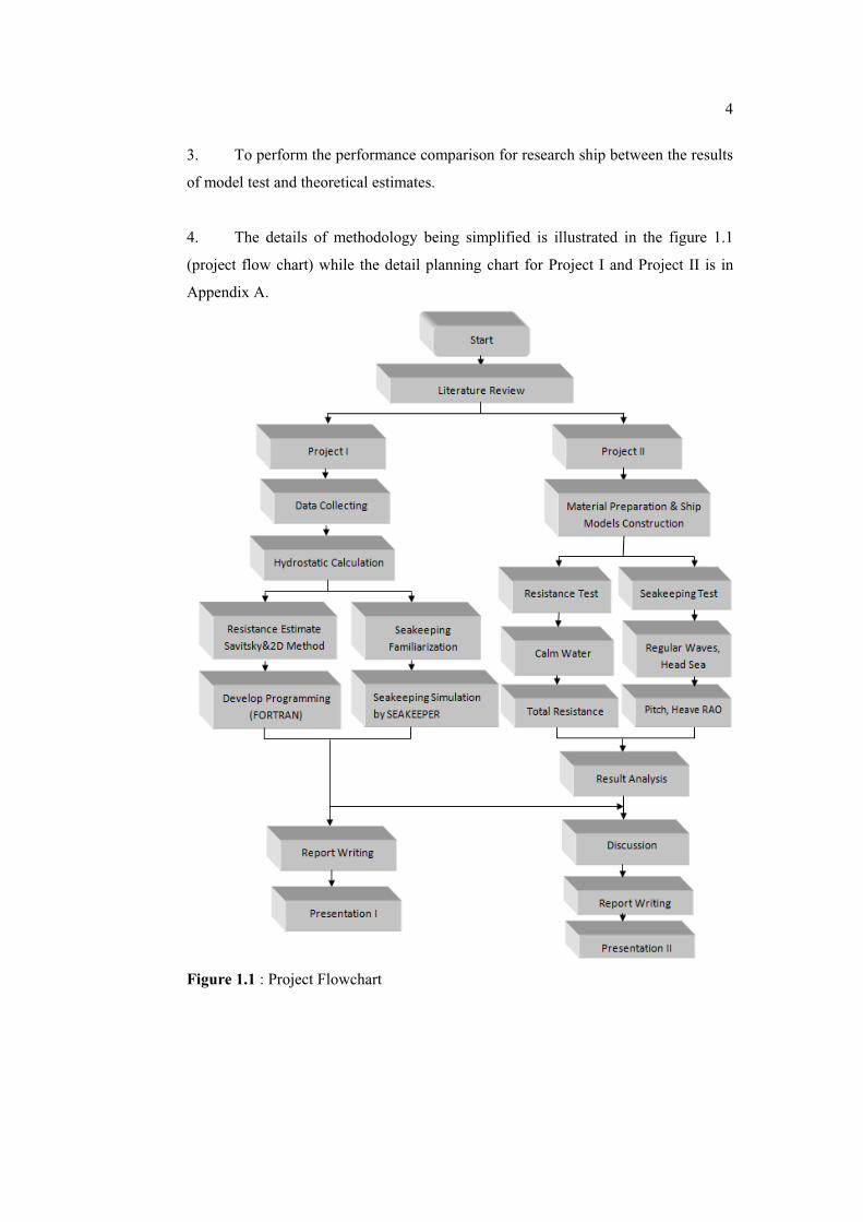
4. The details of methodology being simplified is illustrated in the figure 1.1

(project flow chart) while the detail planning chart for Project I and Project II is in

Appendix A.

Figure 1.1 : Project Flowchart

CHAPTER 2

LITERATURE REVIEW

2.1 Introduction

A high-speed craft (HSC) is a high speed vessel for civilian use, also called a

fast craft or fast ferry and is called patrol craft for military purposes. A vast increase

in high speed crafts due to existing needs in the field of fast transport of light and

expensive cargo, passengers at high speed craft for marine transportation has drawn

considerable interest for both shipowners and naval architectures. The function of

high speed also gives advantages to ships which are design to be used for a

surveillance and patrol in maritime area at open sea. Advanced concept was applied

in many types of high speed craft in order to obtain a great performance in seaway.

The design and safety of high-speed craft is regulated by the High Speed Craft Codes

of 1994 and 2000, adopted by the Maritime Safety Committee of the International

Maritime Organisation (IMO).

Clayton et al [1] defined the high speed craft when the craft speeds are

reached for which hydrostatic force less or equal to pressure force, Fh:Fp, but some

part must be submerged. Therefore wetted length, lk ; 0 and also Fh ; 0. However

this definition is hard to improve which Newton [2] stated that it is generally

recognized that the definition of high speed when the RT/W curve level off and stern

trim has reached maximum. Another definition was identified by Mandel [3] that the

craft to be high speed when it ceases to be buoyantly supported and becomes

completely dynamically supported. Clement and Pope [4] found this occurred when

volume Froude number, Fr�< =>?>

6�

At different perspective, Savitsky et al [5] defined that high speed craft are

considered to be vessels that can travel at a sustained speed equal to or greater than

35 knots with bursts of high speeds of 40-60 knots. Froude number allows for

another way to hydrodynamically classify ships. Naval architects use the Froude

number when vessels deal with the interaction of the water’s free surface and the

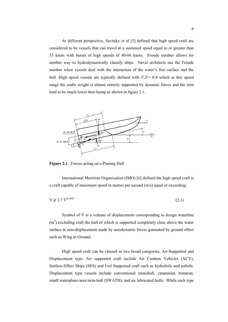
hull. High speed vessels are typically defined with Fn�> 0.4 which at this speed

range the crafts weight is almost entirely supported by dynamic forces and the trim

tend to be much lower than hump as shown in figure 2.1.

Figure 2.1 : Forces acting on a Planing Hull

International Maritime Organization (IMO) [6] defined the high speed craft is

a craft capable of maximum speed in metres per second (m/s) equal or exceeding:

V�<�3.7 �0.1667 (2.1)

Symbol of � is a volume of displacement corresponding to design waterline

(m3) excluding craft the hull of which is supported completely clear above the water

surface in non-displacement made by aerodynamic forces generated by ground effect

such as Wing in Ground.

High speed craft can be classed in two broad categories, Air-Supported and

Displacement type. Air supported craft include Air Cushion Vehicles (ACV),

Surface-Effect Ships (SES) and Foil Supported craft such as hydrofoils and jetfoils.

Displacement type vessels include conventional monohull, catamaran, trimaran,

small waterplane-area twin-hull (SWATH), and air lubricated hulls. While each type

7�

of vessel has its own unique characteristics, they all suffer from the common problem

of limited payload and a sensitivity to wind and sea state.

2.2 Planing Craft

Planing craft are used as patrol boats, sport vessels, service craft and and for

sport competitions. When a vessel is planing, it is mainly supported by

hydrodynamic forces. A length Froude number of 1-1.2 is often used as a lower limit

for planing conditions. There are many important dynamic stability problems

associated with planing vessels such as porpoising stability. Strongly nonlinear

phenomena will appear during planing including spray jet, breaking waves etc.

Therefore it is hard to apply conventional linear theories for displacement vessels to

study planing hulls. In order to accurately predict the hydrodynamic behavior of a

planing vessel, non-linear effects must be included in the analysis. The characteristic

of this crafts was defined by Froude and operates Froude number (Fn) larger than

about 0.4. Generally, the buoyancy force dominates relative to the hydrodynamic

force effect when Fn is less than approximately 0.4. When Fn>1.0, the

hydrodynamic force mainly carries the weight, then the vessel turn into a planing

craft.

A planing hulls are hullforms characterized by relatively flat bottoms and

shallow V-sections (especially forward of amidships) that produce partial to nearly

full dynamic support for light displacement vessel and small craft at higher speeds.

These types of hull form lift and skim the surface of the water causing the stern wake

to break clean from the transom. The crafts are generally restricted in size and

displacement because of the required power-to weight ratio and the structural stresses

associated with traveling at high speed in wave. Most planing hull crafts are also

restricted to operate in reasonably calm water, although some “deep-V” hull forms

are capable operated in rough water. As mentioned in [7], in general there are three

types of planing hulls with different characteristics and advantages. They are

namely;

8�

1. Deep Vee Bottom.

2. Inverted Vee Bottom.

3. Round Bottom.

In Deep Vee Bottom type, single hard chine is most frequently used. This

form has the advantages of being a substantially good planing surface form, simple

and economical to produce and having excellent accommodation space for

machinery, armament, and crew. It has a disadvantage of having a greater wetted

surface with consequent greater resistance. Its characteristics in a seaway compared

to other planing hull forms are only fair. On the contrary, planing hull forms are poor

in rough water [8].

Numerous researches in planing hull seakeeping technology have quantified

the relations between hull form, loading, speed/length ratio, sea state and the

expected added resistance, motions and wave impact accelerations. The process of

optimization of hull form for achieving the ‘best’ hull shape is shown in reference

[9]. The shapes with the best performance at sea, are in terms of hydrodynamic

behaviors, structural robustness, transport efficiency, operational and economic

advantage.

2.2.1 Geometry of Planing Craft

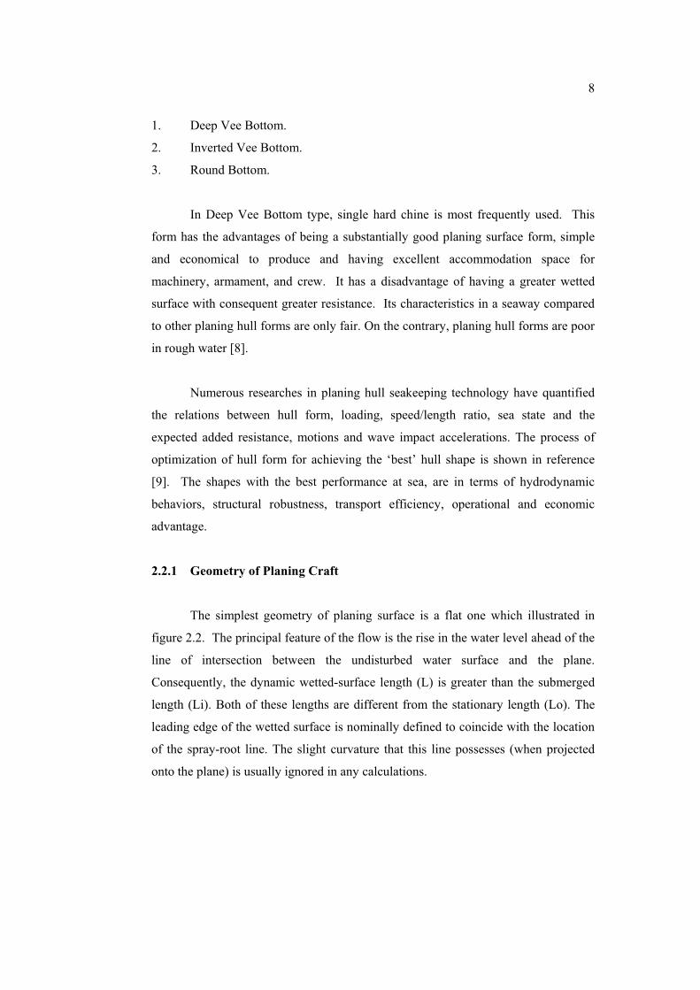
The simplest geometry of planing surface is a flat one which illustrated in

figure 2.2. The principal feature of the flow is the rise in the water level ahead of the

line of intersection between the undisturbed water surface and the plane.

Consequently, the dynamic wetted-surface length (L) is greater than the submerged

length (Li). Both of these lengths are different from the stationary length (Lo). The

leading edge of the wetted surface is nominally defined to coincide with the location

of the spray-root line. The slight curvature that this line possesses (when projected

onto the plane) is usually ignored in any calculations.

9�

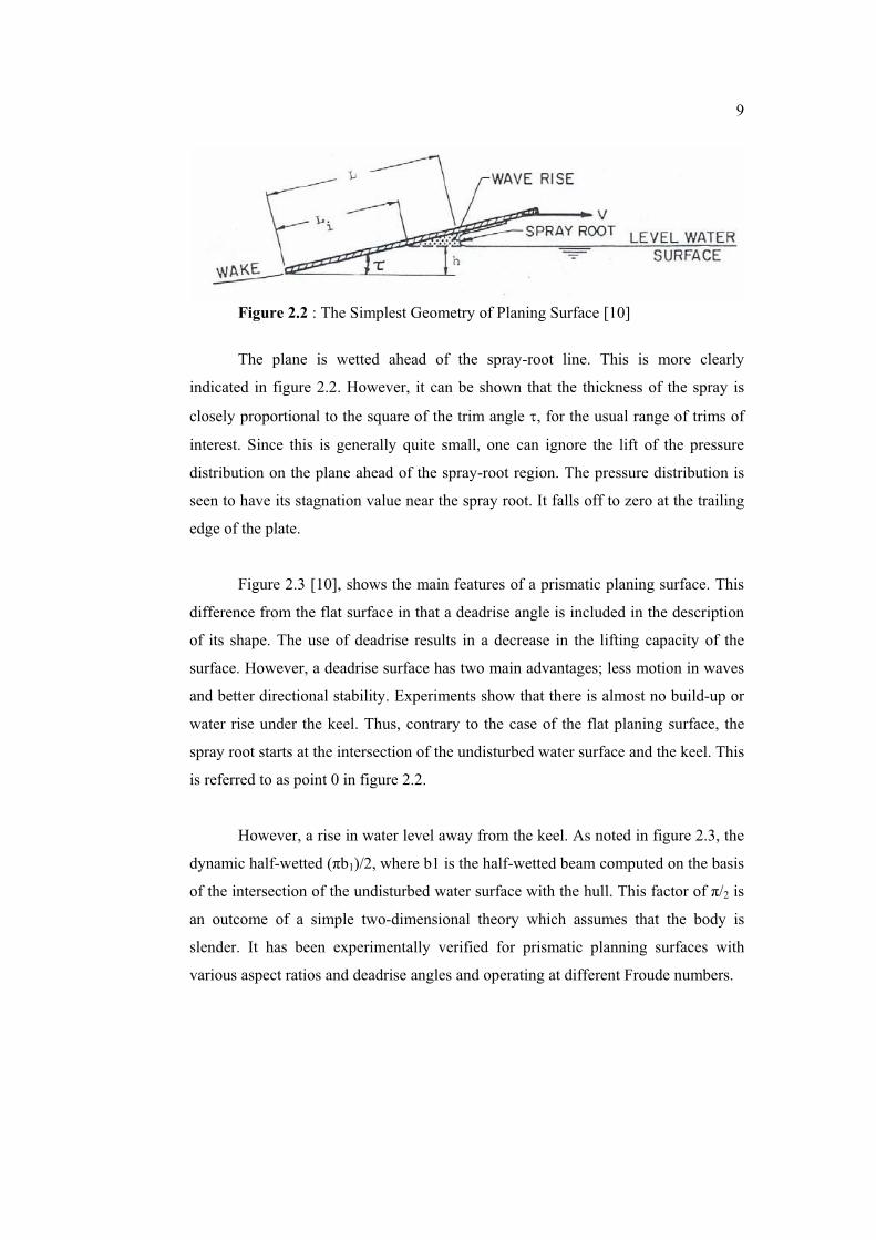
Figure 2.2 : The Simplest Geometry of Planing Surface [10]

The plane is wetted ahead of the spray-root line. This is more clearly

indicated in figure 2.2. However, it can be shown that the thickness of the spray is

closely proportional to the square of the trim angle , for the usual range of trims of

interest. Since this is generally quite small, one can ignore the lift of the pressure

distribution on the plane ahead of the spray-root region. The pressure distribution is

seen to have its stagnation value near the spray root. It falls off to zero at the trailing

edge of the plate.

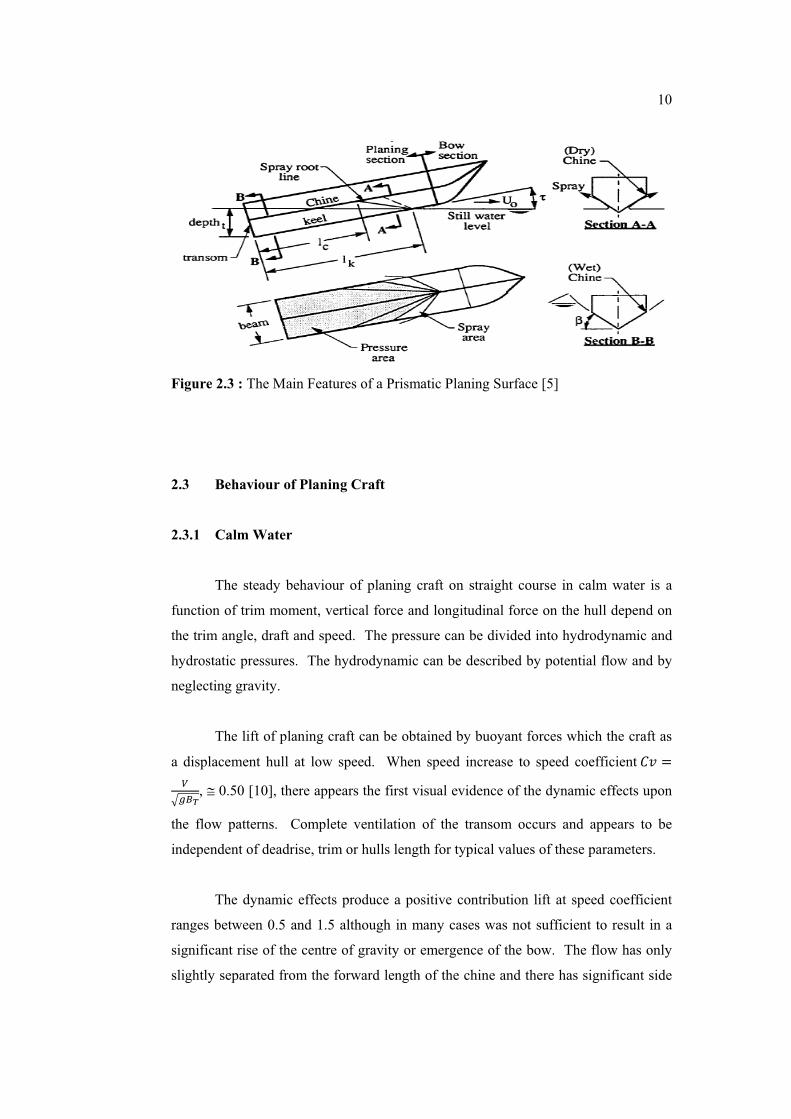
Figure 2.3 [10], shows the main features of a prismatic planing surface. This

difference from the flat surface in that a deadrise angle is included in the description

of its shape. The use of deadrise results in a decrease in the lifting capacity of the

surface. However, a deadrise surface has two main advantages; less motion in waves

and better directional stability. Experiments show that there is almost no build-up or

water rise under the keel. Thus, contrary to the case of the flat planing surface, the

spray root starts at the intersection of the undisturbed water surface and the keel. This

is referred to as point 0 in figure 2.2.

However, a rise in water level away from the keel. As noted in figure 2.3, the

dynamic half-wetted (�b1)/2, where b1 is the half-wetted beam computed on the basis

of the intersection of the undisturbed water surface with the hull. This factor of �/2 is

an outcome of a simple two-dimensional theory which assumes that the body is

slender. It has been experimentally verified for prismatic planning surfaces with

various aspect ratios and deadrise angles and operating at different Froude numbers.

10�

Figure 2.3 : The Main Features of a Prismatic Planing Surface [5]

2.3 Behaviour of Planing Craft

2.3.1 Calm Water

The steady behaviour of planing craft on straight course in calm water is a

function of trim moment, vertical force and longitudinal force on the hull depend on

the trim angle, draft and speed. The pressure can be divided into hydrodynamic and

hydrostatic pressures. The hydrodynamic can be described by potential flow and by

neglecting gravity.

The lift of planing craft can be obtained by buoyant forces which the craft as

a displacement hull at low speed. When speed increase to speed coefficient��@ A��B, � 0.50 [10], there appears the first visual evidence of the dynamic effects upon

the flow patterns. Complete ventilation of the transom occurs and appears to be

independent of deadrise, trim or hulls length for typical values of these parameters.

The dynamic effects produce a positive contribution lift at speed coefficient

ranges between 0.5 and 1.5 although in many cases was not sufficient to result in a

significant rise of the centre of gravity or emergence of the bow. The flow has only

slightly separated from the forward length of the chine and there has significant side

11�

wetting. The planing craft should develop dynamic lift forces when the speed

coefficient larger than 1.5. The lift forces give a significant rise of the centre of the

gravity, positive trim and emergence of the bow and separation of the flow from the

hard chines. The hydrodynamic resistance is due to the horizontal component of the

bottom pressure force and the friction component of the flow over the bottom which

is there is no bow contribution to drag.

The lift force is approximately proportional to the trim angle. If the craft has

hard chines, the separation lines along the hull are well defined along the chines.

Calculation can be made by neglecting the effect of the viscous boundary layer on

the pressure distribution. But this assumption not applicable to the vessel with round

bilges, whereas the separation lines may then be dependent on laminar or turbulent

flow conditions in the boundary layer.

According to Savitsky [10], the lift on the planing surface is attributed to two

separated effects. One is the positive dynamic reaction of the fluid against the

moving planing bottom, and the second one is the so-called buoyant contribution

which is associated with the static pressures corresponding to a given draft and hull

trim. At very low speeds, the buoyant lift predominates, while at high speed, the

dynamic contribution predominates. The lift coefficient, CL is a function of mean

wetted length beam ratio, �.

For a flat planing surface, � = 0o, the lift coefficient is:

�� A � CD>D)E>EFGEH� I J>JJKKLMNO' + (2.2)

Where ��can be obtain by solving equation (2.3) and (2.4)

�� A �� P E>EEQ?R��2J>S (2.3)

�� A � T�UDVWT�'�' (2.4)

12�

Then, any lifting surface or flat plate in a free stream, as well as planing surface or

planing hull, is subjected to lift force:

� A DW ��XWY (2.5)

While other parameters being constant, the hydrodynamic lift varies as the

square of the beam. The planing lift is predominately due to dynamic bottom

pressures when the speed coefficient and Froude number defined above is greater

than 10. The effect of deadrise angle is to reduce the lift coefficient, while all other

factor being equal.

2.3.2 Rough Water

The occurrence of waves has considerable importance on the design of

planing craft and this factor must be included in the prediction of seakeeping at initial

stage of design. The hull form is dependant on the expected wave encounter spectra,

or perhaps the worst wave spectra envisaged, since the new problem must include a

measure of seakeeping ability, so that hull accelerations and response amplitudes can

be determined. It is well known that for planing craft the flat-water/rough water

problem is essentially one of a compromise between speed and seakeeping.

A planing craft running into waves can be considered to be a coupled 3

degree of freedom (heave, pitch and surge) dynamic system wherein the hull is acted

upon by a forcing function generated by the waves it encounters. The dynamic

properties of the hull are represented by the acceleration forces due to its physical

and added mass and moments of inertia; the force and moment acting on the hull due

to a unit displacement in heave or pitch (the so-called spring constants of the hull);

and the force and moment acting on the hull due to its heave or pitch velocity (the so-

called damping forces). The forcing function acting on the hull at a given speed is

due to the interaction of the encountered wave properties (height, orbital velocities,

accelerations, etc.) and the physical geometry of the hull. As expected, this is a

13�

complex non-linear mathematical system even without the force and moment inputs

due to an active control system.

The behaviour of a ship in rough water is fundamentally similarly to the

oscillatory response of the classical damped spring mass system illustrated in figure

2.4. The classical spring mass system consists of a mass a (tonnes) which is

connected to a fixed rigid base through a dashpot and a spring. The dashpot exerts a

damping force b (kN) in response to a velocity of 1 metre/second and the spring

exerts a restoring force c (kN) if the displacement is 1 metre. If the system is not

disturbed it will adopt an equilibrium position which we shall define as a datum

displacement, x=0 (m).

Figure 2.4 : Spring Mass System [11]

The total force F was applied to the mass at any instant of time which related

to the motion by the equation:

Fcxdtdxb

dtxda ��2

2

(2.6)

The first term is the force acting on the system due to acceleration of the

physical mass, a and the added mass; the second term is the force due to damping of

14�

the system taken to be linearly dependent upon the normal velocity of the hull and

the damping coefficient,b , the third term is the force due to displacement where c is

the effective spring constant of the hull. The term on the right hand side is the force

F assumed to be acting on the system. The natural frequency �� of the system can

be simplified by neglecting the damping which gives a small effect to the system.

The natural frequency can be expressed as:

�� A Z�[ (2.7)

For the steady condition the amplitude response can be expressed in non dimensional

form as:

\J A \!]^ (2.8)

Where: ^ = Magnification factor \!] = �#�

0F = Force acting on body ^ = _#_`a ��A DZbDc�'d'e �'�' (2.9)

� = Tuning factor, ��f

� = Non dimensional damping factor, �WH�[

Thus the phase response can be expressed in non dimensional form as:

g A h5icD W��Dc�' (2.10)

The amplitude of the response of a linear spring mass system is show in the

form of a classic plot that readily quantifies the response of a dynamic system to a

15�

sinusoidal forcing function. The plot of amplification factor versus ratio of applied

frequency of forcing function /natural frequency of the dynamic system as a function

of the damping ratio of the system is shown in figure 2.5.

Figure 2.5 : Response of a Linear Spring Mass System [11]

In terms of ship motion terminology, the magnification factor can be likened

to the response amplitude operator (RAO), i.e. considering heave motion; the RAO is

the ratio of the magnitude of heave of the craft to the height of the wave that caused

this heave motion. Likewise this RAO can also represent the ratio of craft pitch

amplitude to the slope of the wave that caused the craft to pitch. There is a separate

curve for different values of damping ratio. It is noticed that the RAO decreases

rapidly with increasing damping ratio particularly at resonance (�=�n). At super-

critical damping ratios � < 0.70, the RAO is < 1.0 so that the heave and pitch

motions will actually be less that the disturbing wave height or wave slope. The

maximum RAO occur at all damping ratios when the frequency of wave encounter is

equal to the natural frequency of the craft (resonant condition).

� =0.707

� =0.5

� =0.1

� =0.25

� =0.05

� =0

10V�8�

5V�c�

1V�8�

16�

2.4 Hydrodynamic forces on Planing Craft

The first step in describing the hydrodynamic behaviour of high speed craft

(planing) is made by an analysis of the influence of the main design parameters, such

as length to beam ratio, deadrise angle, displacement and LCG, on the calm water

resistance of the hull. Because the running trim is also important for the vertical

accelerations in waves both the sinkage and the running trim of the craft at speed are

analyzed too. This research was carried out in a number of steps by Gerritsma and

Keuning [12,13]. They extended the original Series 62 experiments as, carried out by

Clement and Blount [14], with a large number of similar models but now with 19, 25

and 30 degrees of deadrise of the planing bottom respectively.

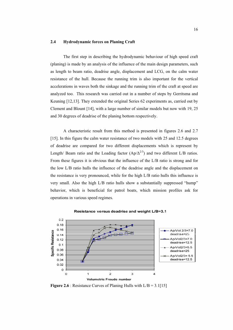
A characteristic result from this method is presented in figures 2.6 and 2.7

[15]. In this figure the calm water resistance of two models with 25 and 12.5 degrees

of deadrise are compared for two different displacements which is represent by

Length/ Beam ratio and the Loading factor (Ap/�2/3) and two different L/B ratios.

From these figures it is obvious that the influence of the L/B ratio is strong and for

the low L/B ratio hulls the influence of the deadrise angle and the displacement on

the resistance is very pronounced, while for the high L/B ratio hulls this influence is

very small. Also the high L/B ratio hulls show a substantially suppressed “hump”

behavior, which is beneficial for patrol boats, which mission profiles ask for

operations in various speed regimes.

Figure 2.6 : Resistance Curves of Planing Hulls with L/B = 3.1[15]

17�

Figure 2.7 : Resistance Curves of Planing Hulls with L/B = 7.0 [15]

From the hump behaviour of the L/B = 2 ship and its lower resistance at the

highest speeds it may also be concluded that the hydrodynamic lift plays a much

bigger role with these ships when compared to the higher L/B ratio hulls. This is a

known phenomenon with planing hulls where the L/B ratio may be considered as

inversely related to the aspect ratio of a wing analogue.

The formulations of the hydrodynamic forces acting on high speed craft

sailing in waves used in the present report are largely based on the mathematical

model as first presented by Zarnick [16] and later further extended by amongst others

by Keuning [17,18]. In the present report the formulations will be restricted to a

short summary. The complete set of formulations of all forces involved may be

found in these References. The development of both the hydrostatic and

hydrodynamic lift forces on a fast moving ship is described by making use of a strip

theory type approach. Dividing the ship in an arbitrary number of segments along its

length (strips) the force on each of the segments may be considered to be constituted

of a hydrostatic component related to the displaced water, a dynamic component

related to the change of momentum of the incoming fluid and a viscous part, i.e.:

�. A ��] )j[@+ I �k�l7@W P 5�mln(8op� (2.11)

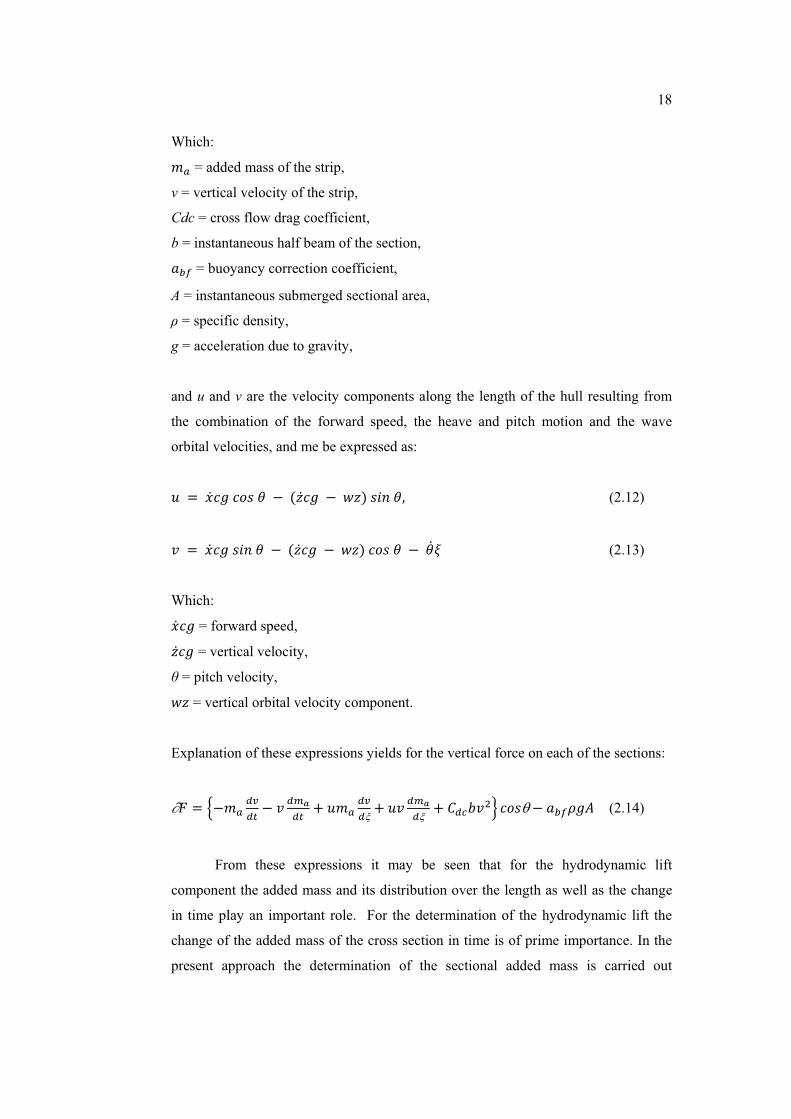
18�

Which: j[ = added mass of the strip,

v = vertical velocity of the strip,

Cdc = cross flow drag coefficient,

b = instantaneous half beam of the section, 5�m = buoyancy correction coefficient,

A = instantaneous submerged sectional area,

� = specific density,

g = acceleration due to gravity,

and u and v are the velocity components along the length of the hull resulting from

the combination of the forward speed, the heave and pitch motion and the wave

orbital velocities, and me be expressed as:

q� A �\38n�8op�*� P�)038n� P ��0+�pri�*2 (2.12) �@� A � \38n�pri�*� P�)038n� P ��0+�8op�*� P�*3s (2.13)�

Which: \38n = forward speed, 038n = vertical velocity,

� = pitch velocity, �0 = vertical orbital velocity component.

Explanation of these expressions yields for the vertical force on each of the sections:

�. A tPj[ k�k] P @ kuvk] I qj[ k�k�I q@ kuvk�

I �k�7@Ww 8op� P 5�mln( (2.14)

From these expressions it may be seen that for the hydrodynamic lift

component the added mass and its distribution over the length as well as the change

in time play an important role. For the determination of the hydrodynamic lift the

change of the added mass of the cross section in time is of prime importance. In the

present approach the determination of the sectional added mass is carried out

19�

considering it to be directly related to the instantaneous maximum submerged

maximum beam of the section under consideration, which is additionally corrected

for the “pile-up” of the water in the dry chine sections. The expression for added

mass following Wagner’s approach then reads:

j[ �A DW �lx7Wy[ (2.15)

Whereas y[ is a coefficient, which may be determined for each section and

which is dependent on the beam to draft ratio and the deadrise angle. The magnitude

of 5�m�and y[ are determined separately in the steady state equilibrium condition and

considered constant also for the motions in waves. Due to the fact that in a non-

linear approach the relative motion of the ship with respect to the disturbed water

surface is no longer considered to be small, the change of shape of the actual

submerged part of the cross section is taken into account. By doing so the change in

added mass in time, needed in the formulation of the hydrodynamic lift, is taken into

account. In the present approach the added mass of each section of the fast ship is

considered to be frequency independent. On the other hand the added mass is taken

to be dependent on the actual momentaneous submerged geometry of the section and

so very much time dependent. The validity and the importance of such an approach

for the assessment of the hydrodynamic lift forces on the planing hull, is

demonstrated by Keuning [18]. The cross flow drag term is determined using the

instantaneous value of the normal velocity component on each of the sections. The

cross flow drag coefficient �k� is determined using the work of Shuford for V shaped

sections and is:

�k� = 1.30 cos � in which: � = the deadrise angle of the sections.

In general it is found that this cross flow drag is of minor importance when

compared with the other forces involved. Due to the dynamic lift and the flow

separation over at least a part of the chine’s and the entire transom the buoyancy

force, which is determined supposing hydrostatic pressure distribution, needs a

correction. The buoyancy related lift therefore is corrected by a correction

coefficient. This correction coefficient is 5�m and in the present approach this 5�m is

20�

assumed to be the same for all sections along the length of the ship were

displacement of water is present. In the computer code FASTSHIP developed by the

Delft Shiphydromechanics Department for the calculation of the heave and pitch

motions of fast ships in irregular waves, see [18], the values of y[ and 5�m are

determined from the equilibrium condition of the craft at speed in calm water (no

waves). For this particular condition the running trim (pitch) and the sinkage (heave)

of the ship are determined from the results of the Delft Systematic Deadrise Series

(DSDS), see [13]. Combining these results with the forces calculated in the equations

of motions the unknowns can be solved.

One other source for the non-linear behaviour of the planing hull in waves

may be found in the wave exciting forces. These originate from the large relative

motions that these craft perform with respect to the incoming waves. From the

research as reported by Keuning [17] it was revealed that the wave exciting forces on

a fast monohull sailing in waves are dominated by the non-linear Froude Kriloff

component. This is an important conclusion when these non-linear wave-exciting

forces are to be calculated in a time domain solution, in which no frequency

dependency can be accounted for. This non-linear Froude Kriloff force is calculated

by integration of the dynamic pressure in the undisturbed incoming wave over the

actual momentaneous submerged area of the hull whilst performing large amplitude

relative motions with respect to the disturbed water surface. For this calculation the

full geometry of the hull from keel to deck is being used. The expression used yields:

.z{ A Gln4�� P lny(� (2.16)

Which: .z{ = Froude Kriloff force on section,

� = specific density of water, 4� = momentaneous beam section on the waterline (time dependent),

� = wave height (time dependent),

k = wave number,

A = momentaneous submerged area of section

21�

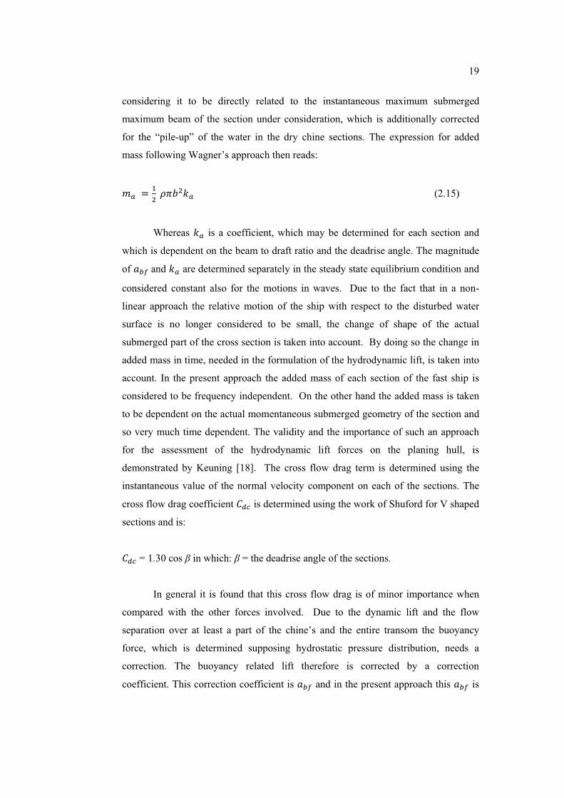
2.5 Transom or Stern Flap Performance

Practically, transom or stern flaps have been used on many high-speed craft,

such as survey vessel, surveillance and patrol craft, and pleasure craft [19]. A

transom flap represents an extension of the hull aft of the transom in the form of a

flat plate. The flap is incorporated to the transom at an angle relative to the

centreline buttock of the ship [20], as in figure 2.8 and 2.9. Every transom flaps,

independent of what vessels size or type they are used on, create a vertical lift force

at the transom, and modify the pressure distribution on the after portion of the hull.

The modification of the afterbody flow field causes the principal performance

enhancement on a hull.

A transom flap create the flow to slow down under the hull at a location

extending from its position to a point generally forward of the propellers. This

decreased flow velocity will cause an increase in pressure under the hull, which in

turn, causes reduced resistance due to the reduced afterbody suction force (reduce

form drag). Wave heights in the near field stern wave system, and far field wave

energy, are both reduced by these devices. Localized flow around the transom,

which represents lost energy through eddy making, wave breaking, and turbulence, is

significantly modified by the stern flap. The flow exit velocity from the trailing edge

of the flap is increased in comparison with the baseline transom, leading to a lower

speed for clean transom flow separation, and again, reduced resistance [21].

Secondary effects of the transom flap include the lengthening of the hull,

improved propeller-hull interactions, and improved propeller performance due to

reduced loading, and reduced cavitations tendencies.

22�

Figure 2.8 : The location of Stern Flap [22]

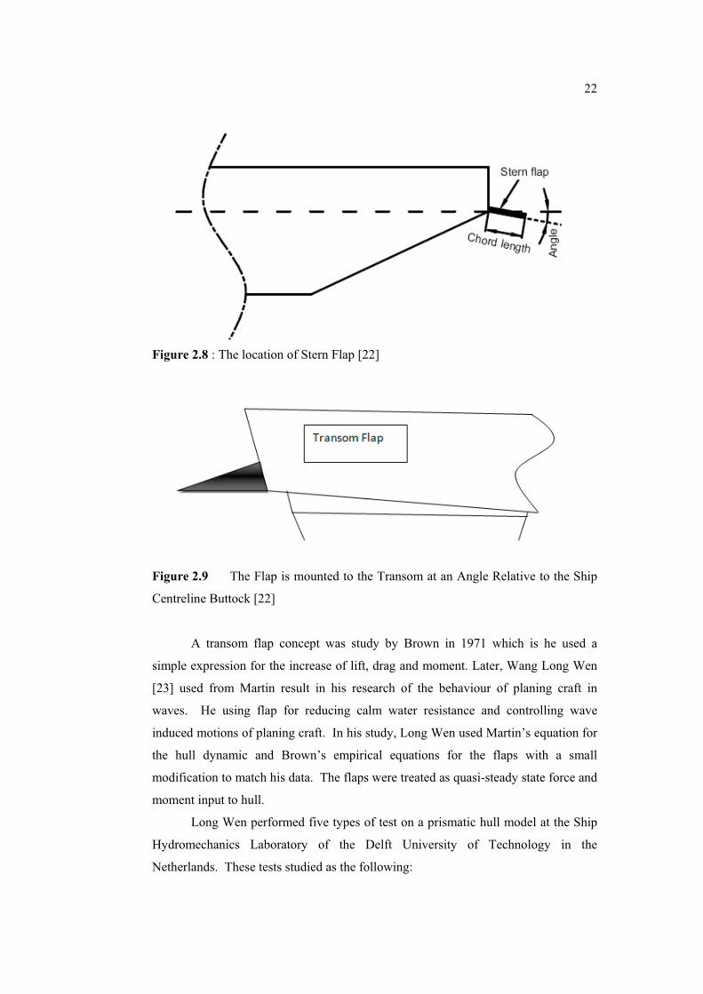
Figure 2.9 The Flap is mounted to the Transom at an Angle Relative to the Ship

Centreline Buttock [22]

A transom flap concept was study by Brown in 1971 which is he used a

simple expression for the increase of lift, drag and moment. Later, Wang Long Wen

[23] used from Martin result in his research of the behaviour of planing craft in

waves. He using flap for reducing calm water resistance and controlling wave

induced motions of planing craft. In his study, Long Wen used Martin’s equation for

the hull dynamic and Brown’s empirical equations for the flaps with a small

modification to match his data. The flaps were treated as quasi-steady state force and

moment input to hull.

Long Wen performed five types of test on a prismatic hull model at the Ship

Hydromechanics Laboratory of the Delft University of Technology in the

Netherlands. These tests studied as the following:

23�

1. The effect of full width flaps on resistance, lift and trim for speed coefficient

between 2.3 to 2.9 and flap angles between 0o to 3o.

2. The forces and moments on the flap for flap length to beam ratios between

8.3% to 16.7% and flap angles between 0o to 9o.

3. The responses of the model when excited by oscillating flaps.

4. The responses of the model without controllable flaps when excited by waves

with wave length to vessel length ratios 1 to 6.

5. The responses of the model with controllable flaps when excited by waves

with wave length to vessel length ratios 1 to 6.

The results from model tests were very positive. The calculations and

experiment results had very good agreement for all of the tests performed. The flaps

were useful for reducing the steady state resistance and for controlling the wave

induced motions of a planing craft.

2.6 Theory of Foil

Motion control may be effective by reducing the heave and pitch of a high

speed vessel especially in planing hull. In order to decrease these motions, the foil

was effective technique rather than other methods. Basically the foil system was

similar concept with trim tab, transom flap and interceptor which to reduce the heave

and pitch motion and also to optimise the resistance. By adapting the foil, the

damping of heave and pitch will be increased that resulting the reducing of the heave

and pitch motions. Normally the foil was placed at the bow of the vessel because the

vertical motions are largest at this area. But in this case, the foil was modifying by fit

in below aft of the vessel in order to improve the seakeeping capability and

maintained her cruising speed 25 knots at minimum sea state code 3.

The study will be focused on submerged foil which it gives an advantage in

avoiding slamming, cavitation and ventilation. However, the cavitation and

ventilation depends on the local flow around the flow which is affected by foils

24�

design, the angle of attack of the incident flow to the foil and also foil motions. The

higher the ship speed, the larger probability of the cavitation and ventilation cause of

this foils add drag to the vessel. The effect of foil system will result reducing the

trim angle which contributes the good seakeeping. The phasing flap angles can be

controlled relative to trim angle () which is cause by a pressure distribution on the

hull and would result a trim moment on the vessel that reduces trim angle at high

speed condition. It also shows that the dynamic lifting force become most significant

and the seakeeping characteristics are considerably different which is given a great

influence to the ship performance.

The trim angle of the vessel can be determined by considering the lift

coefficient of the foils. Lift coefficient for foil system depend on many parameters,

such as:

1. Angle of attack (�) of the incident flow.

2. Flap angles, (�).

3. Camber (f).

4. Thickness to chord ratio.

5. Aspect ratio (�).

6. Ratio between foil submergence, h and maximum chord length,c.

7. Submergence Froude Number.

8. Interaction from upstream foils.

9. Cavitation number.

10. Reynolds number.

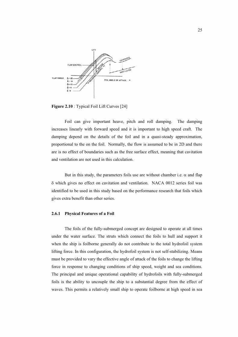
The steady lift force depends on � and �. When � and � are small, the

linearly dependent on � and �. If the foil has a camber, the lift is non-zero when �

and � are zero. However, � or � are large then cavitation and ventilation will be

materialized which it depending on speed and submerged of the foils. Refer to figure

2.10, the substantial decrease in lift as a consequence of ventilation. The magnitude

of lift force with cavitation depends on the cavitation number. The suction side of

the foil may be partially or fully cavitating, which partially cavitating may lead to

unsteady lift forces.

25�

Figure 2.10 : Typical Foil Lift Curves [24]

Foil can give important heave, pitch and roll damping. The damping

increases linearly with forward speed and it is important to high speed craft. The

damping depend on the details of the foil and in a quasi-steady approximation,

proportional to the on the foil. Normally, the flow is assumed to be in 2D and there

are is no effect of boundaries such as the free surface effect, meaning that cavitation

and ventilation are not used in this calculation.

But in this study, the parameters foils use are without chamber i.e. � and flap

� which gives no effect on cavitation and ventilation. NACA 0012 series foil was

identified to be used in this study based on the performance research that foils which

gives extra benefit than other series.

2.6.1 Physical Features of a Foil

The foils of the fully-submerged concept are designed to operate at all times

under the water surface. The struts which connect the foils to hull and support it

when the ship is foilborne generally do not contribute to the total hydrofoil system

lifting force. In this configuration, the hydrofoil system is not self-stabilizing. Means

must be provided to vary the effective angle of attack of the foils to change the lifting

force in response to changing conditions of ship speed, weight and sea conditions.

The principal and unique operational capability of hydrofoils with fully-submerged

foils is the ability to uncouple the ship to a substantial degree from the effect of

waves. This permits a relatively small ship to operate foilborne at high speed in sea

26�

conditions normally encountered while maintaining a comfortable motion

environment for the crew and passengers and permitting effective employment of

equipment. Example of classification used for foil is presented in figure 2.11 which

described the parameter of every section of foil.

Figure 2.11a : Foil Parameters Plan View[24]

Figure 2.11b : Foil Parameters Sectional View[24]

2.6.2 Selection of Foil and Strut

In this study, the selection of foil and strut only put on the stern of the vessel

in order to reduce the couple heave and pitch and also to optimize the resistance. By

using the theory of hydrofoil vessel on fully submerged foil system, the planing craft

with M-Hull can reduce the motion and resistance will be optimized in specific speed

at regular waves. Figure 2.12 show the classical of foil configuration that has been

used in design application. The foil are able to support the weight of the vessel at

maximum speed either forward or aft foil. However, from time to time the foil

system also has great improvement in term of size, geometry and function according

to certain vessel.

27�

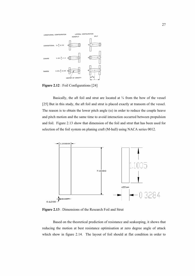
Figure 2.12 : Foil Configurations [24]

Basically, the aft foil and strut are located at ¾ from the bow of the vessel

[25] But in this study, the aft foil and strut is placed exactly at transom of the vessel.

The reason is to obtain the lower pitch angle (�) in order to reduce the couple heave

and pitch motion and the same time to avoid interaction occurred between propulsion

and foil. Figure 2.13 show that dimension of the foil and strut that has been used for

selection of the foil system on planing craft (M-hull) using NACA series 0012.

Figure 2.13 : Dimensions of the Research Foil and Strut

Based on the theoretical prediction of resistance and seakeeping, it shows that

reducing the motion at best resistance optimisation at zero degree angle of attack

which show in figure 2.14. The layout of foil should at flat condition in order to

28�

avoid the cavitations occur which affected the performance of the vessel in term of

resistance and motion.

Figure 2.14 : Resistance and Motion Optimisation at 0o Angle of Attack [24]

The minimum drag condition occurs for angles of leeway or attack of less

than 2 degrees. Beyond 2 degrees, friction drag rises rapidly. The ambient flow

velocity is assumed small relative to the speed of sound that is the fluid may be

considered incompressible. Figure 2.15 shows drag plotted in curves equivalent to

the lift-coefficient curve. As can be seen, drag can also be expressed as a coefficient.

Figure 2.15 : The Drag Coefficient as a Function of angle of attack (leeway) [25]

�

CHAPTER 3

METHODOLOGY

3.1 Introduction

The main purpose of this research is to obtain the most favourable resistance

and to improve the feasibility and effectiveness of the stern foil as means of pitch and

heave reducing. The research is conducted to proof that by incorporating the stern

foil, it will reduce the heave and pitch motion which resulted in good performance on

the vessel. In this research methodology approaches categorized into the theoretical

prediction for resistance by using Savitsky method and seakeeping predictions for the

response heave and pitch motion of vessel is using the strip theory (Geritsma and

Beukelman II Added Resistance Method).

Basically the methodology of this study is separated into two different areas

whereas explained as follows:

3.2. Resistance

The study will be focused on theoretically for predicting the resistance of

with and without stern foil. Prediction of resistance of the vessel will be compute by

using FORTRAN software which the source code of this program based on Savitsky

method for hull and 2D formulations for foil and strut. The calculation will

30��

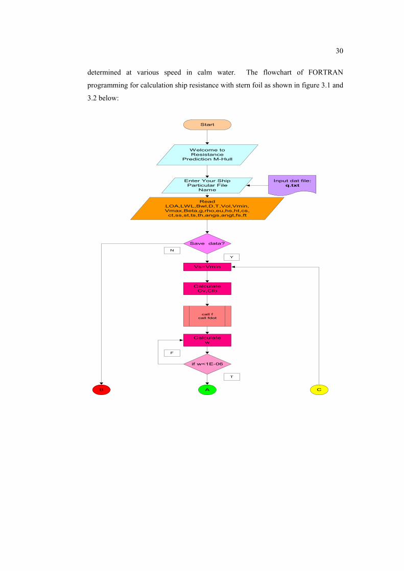
determined at various speed in calm water. The flowchart of FORTRAN

programming for calculation ship resistance with stern foil as shown in figure 3.1 and

3.2 below:

Start

Welcome toResistance

Prediction M-Hull

Enter Your ShipParticular File

Name

ReadLOA,LWL,Bwl,D,T,Vol,Vmin,Vmax,Beta,g,rho,eu,hs,ht,cs,ct,ss,st,ts,th,angs,angt,fs,ft

Input dat file:q.txt

Save data?

Vs=Vmin

Y

N

CalculateCv,Clb

call fcall fdot

Calculatew

if w<1E-06

T

F

AB C

31��

call fcall fdot

Calculateclo

if w<1E-07

T

F

Calculatetrim

call rads

Calculatecorw,RF,RW,RtFoil,

RtStrut

CalculateRt hull

if w<1E-07

TF

Data Saved InData NotSaved

End Program

output data file:output.txt

AB C

Vmin=Vmin+1

Figure 3.1 : The Flowchart of FORTRAN Programming for Resistance Prediction

32��

Subroutine f

X=0.7925xBwlxw^3x-2.39xcgxw^2+3.905xBwlxCv^2xw-5.21xcgxCv^2

Return

Subroutine fdot

Y=2.3775xBwlxw^2x-4.78xcgxw+3.905xBwlxCv^2

if w=0

Y=3.905xCv^xBwl

Return

TF

Subroutine k

A=clo-(0.0065xBetaxclo^0.6)-Clb

Return

Subroutine kdot

B=1-0.0039xBetaxclo^-0.4

if clo=0

B=1

Return

TF

Return

SubroutineRads(Radian)

Radian=PI/180

Figure 3.2 : The Flowchart Subroutine of FORTRAN Programming for Resistance

Prediction

In term of experiment, the resistance test was carried out by using towing

carriage facilities at Marine Technology Laboratory, Universiti Teknologi Malaysia.

The experiment method is utilized for two difference modes of test with and without

33��

stern foil at various speeds in calm water condition. The procedure of resistance test

is described in Appendix B. The flowchart of resistance test procedure is shown in

figure 3.3 below:

Start

Determine the model weight(Law Similarity)

Determine the model LCG andweight ballast using swing frame

Heeling check of the modelinto basin

Attach the model to towing carriage(connect transducers&towing guide,

gimbal )

Run the model atrequired speed

Continuethe test

Do next test fordifferent speed

Transfer the data from DAAS toExcel data

Analize result & Plot graphRT vs Vs & PE vs Vs

Continuethe test

Model Preparation

Stop

Do next test for differentmodel (with stern foil)

N

Y

N

Y

Figure 3.3 : The Resistance Test Procedure

34��

3.3 Seakeeping

For seakeeping analysis, the study is to examine of motions criteria which

dominate in high speed region such as heaving and pitching. The characteristic of

the motions will investigate in strip theory method which using computational

method Maxsurf SEAKEEPER in early prediction of these motions. SEAKEEPER

used Strip Theory (Geritsma and Beukelman II Added Resistance Method) [26] to

predict the coupled of heave and pitch response of a vessel in a seaway. To calculate

the global equations of motions the vessel is split into tranverse sections. These are

treated as two-dimensional sections in order to compute their hydrodynamic

characteristics and these are then integrated along the length of the vessel to obtain

global coefficients of motions.

The prediction using SEAKEEPER validates the motions result of hull form

incorporating with and without stern foil of the vessel respectively. As a preliminary

requirement, offset data of the particular hull need to be prepared in MSD file format.

The supplementary of the offset data together with principal particulars and some

basic hydrostatic data would make the Maxsurf SEAKEEPER predicts the

seakeeping analysis. The module [26] able to generate data on the following

analysis;

1. Regular Response

2. Irregular Response

3. Added Resistance

4. Dynamic Loads

5. Motion Sickness Index

The Maxsurf SEAKEEPER module is considered as a part of frequency

domain based and applies Strip’s theory in order to perform analysis in regular and

irregular wave conditions. This analysis has been undertaken at the top of sea state

code four, which has a characteristic wind speed of 20 knots. Using a Pierson-

Moskowitz spectrum, the wave spectrum has the following details:

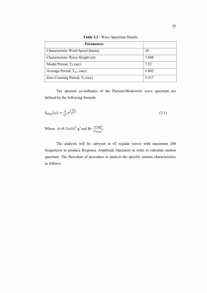
35��

Table 3.1 : Wave Spectrum Details

Parameters

Characteristic Wind Speed (knots) 20

Characteristic Wave Height (m) 1.848

Modal Period, T0 (sec) 7.52

Average Period, Tave (sec) 5.802

Zero Crossing Period, Tz (sec) 5.317

The spectral co-ordinates of the Pierson-Moskowitz wave spectrum are

defined by the following formula:

Y|}�)~+ A �� $ (3.1)

Where A=8.11x10-3

g2and B=

J>� �'��f��

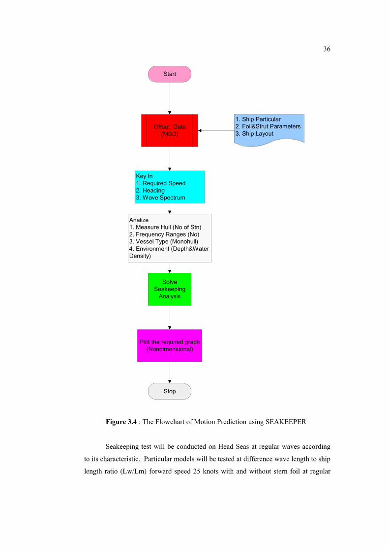
The analysis will be carryout in 63 regular waves with maximum 200

frequencies to produce Response Amplitude Operators in order to calculate motion

spectrum. The flowchart of procedure to analyze the specific motion characteristics

as follows:

36��

Start

Offset Data(MSD)

1. Ship Particular2. Foil&Strut Parameters3. Ship Layout

Key In1. Required Speed2. Heading3. Wave Spectrum

Analize1. Measure Hull (No of Stn)2. Frequency Ranges (No)3. Vessel Type (Monohull)4. Environment (Depth&WaterDensity)

SolveSeakeeping

Analysis

Plot the required graph(Nondimensional)

Stop

Figure 3.4 : The Flowchart of Motion Prediction using SEAKEEPER

Seakeeping test will be conducted on Head Seas at regular waves according

to its characteristic. Particular models will be tested at difference wave length to ship

length ratio (Lw/Lm) forward speed 25 knots with and without stern foil at regular

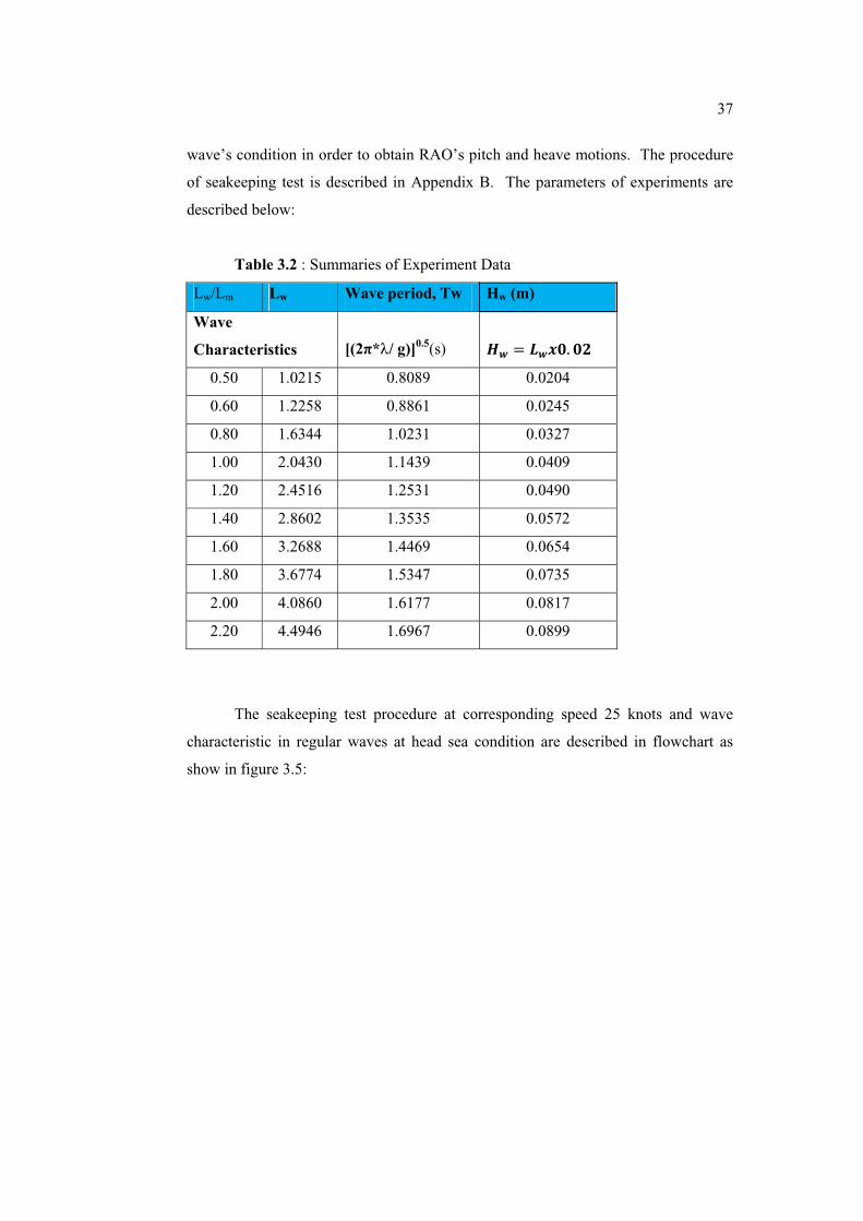
37��

wave’s condition in order to obtain RAO’s pitch and heave motions. The procedure

of seakeeping test is described in Appendix B. The parameters of experiments are

described below:

Table 3.2 : Summaries of Experiment Data

Lw/Lm Lw Wave period, Tw Hw (m)

Wave

Characteristics [(2�*/ g)]0.5(s) �� A ��> �M

0.50 1.0215 0.8089 0.0204

0.60 1.2258 0.8861 0.0245

0.80 1.6344 1.0231 0.0327

1.00 2.0430 1.1439 0.0409

1.20 2.4516 1.2531 0.0490

1.40 2.8602 1.3535 0.0572

1.60 3.2688 1.4469 0.0654

1.80 3.6774 1.5347 0.0735

2.00 4.0860 1.6177 0.0817

2.20 4.4946 1.6967 0.0899

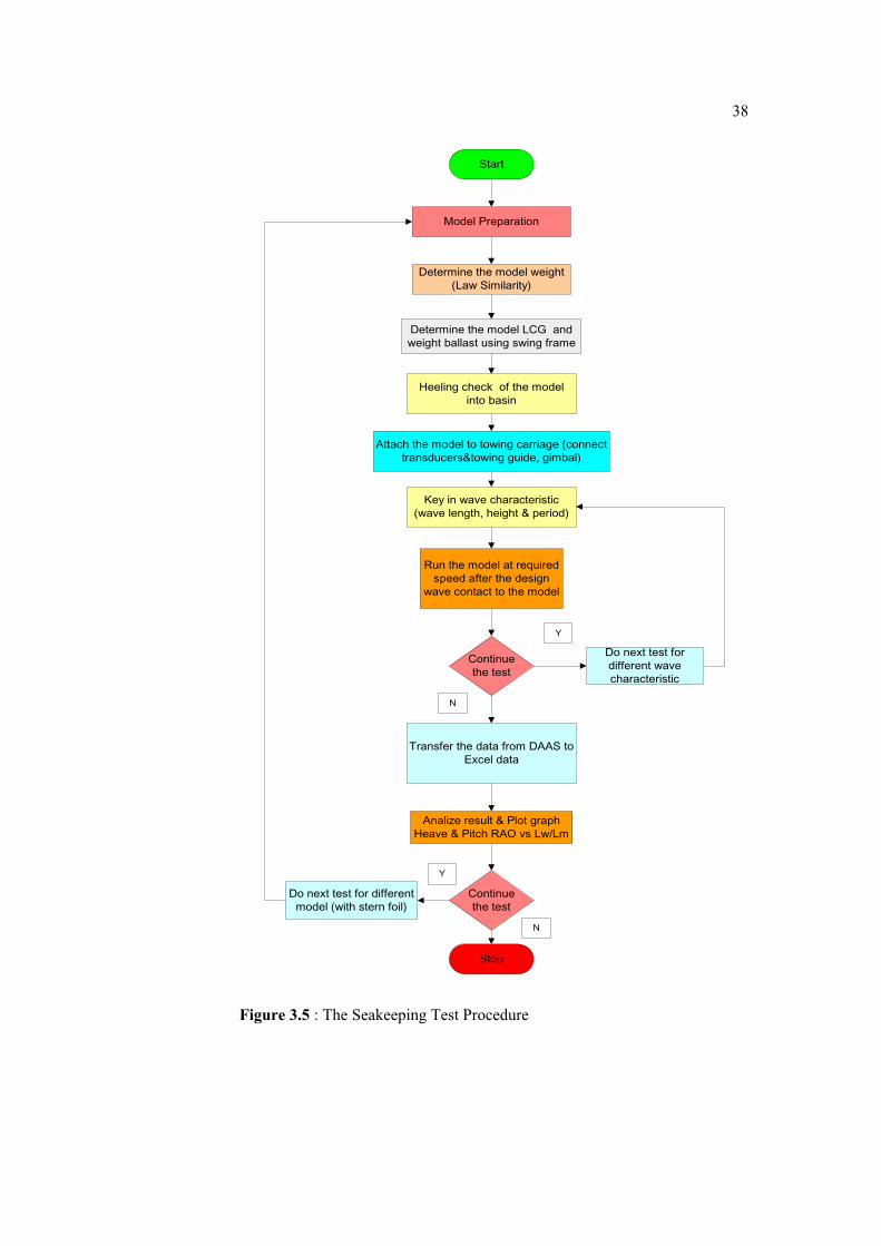
The seakeeping test procedure at corresponding speed 25 knots and wave

characteristic in regular waves at head sea condition are described in flowchart as

show in figure 3.5:

38��

Start

Determine the model weight(Law Similarity)

Determine the model LCG andweight ballast using swing frame

Heeling check of the modelinto basin

Attach the model to towing carriage (connecttransducers&towing guide, gimbal)

Run the model at requiredspeed after the design

wave contact to the model

Continuethe test

Do next test fordifferent wavecharacteristic

Transfer the data from DAAS toExcel data

Analize result & Plot graphHeave & Pitch RAO vs Lw/Lm

Continuethe test

Model Preparation

Stop

Do next test for differentmodel (with stern foil)

N

Y

N

Y

Key in wave characteristic(wave length, height & period)

Figure 3.5 : The Seakeeping Test Procedure

39��

3.4 Concluding Remarks

The procedure in theoretically and experimentally basis are important to

ensure that project outline are in scope of work and method that has been used to

materialized the research. In this case, the resistance and seakeeping test were

conducted in order to validate the theoretically prediction and to check the ship

behaviour at specific speed and wave characteristic.

�

CHAPTER 4

RESISTANCE

4.1 Introduction

There are numerous methods available today by which a ship designer can

obtain an estimate of the resistance of high speed craft. Studies made by various

authors and the present study show that no single method is accurate to predict the

resistance over a wide range of speeds. Research made over the last few years show

that some of the modern regression methods are sufficiently accurate over the speed

range for which they had been developed while some of the other methods have been

less than satisfactory. While using regression methods designers generally tend to

satisfy the non-dimensional range for their particular hullform. The most important

aspect i.e., the hull shape needs to be considered bearing in mind the limitations

applicable to a particular method. To ensure confidence in accuracy it is imperative

to investigate the regression methods in detail and compare results of a number of

vessels for whom models have been previously tested.[27]

Generally, perhaps the most significant contributor to good prediction

reliability is the appropriate selection of the prediction method. The selected

prediction method should be built from hulls that share the same basic character as

the vessel under review. Referring to drawings of the method’s hull forms is the first

step to selecting a suitable method. After principal hull type, the method’s range of

data set parameters must be considered. The most critical parameter to watch is speed

(typically Froude number), then the hull form parameters. The obvious way to avoid

41

difficulty is to evaluate many different methods and to select one that offers a good

correlation between a ship and the method.

4.2 Resistance Components

Figure 4.1 : Breakdown of Resistance into Components

The resistance of a surface vessel may be separated into components

attributed to different physical processes, which scale according to different scaling

laws. Such a breakdown is presented in figure 4.1. The resistance of a vessel

(neglecting air resistance) is due to shear and normal fluid stresses acting on the

vessel's underwater surface. The shear stress component is entirely due to the

viscosity of the fluid, whilst the normal stress component may be separated into two

major components: wave making, due to the generation of free surface gravity waves

(inviscid) and a viscous pressure component caused by the pressure deficit at the

stern due to the presence of the boundary layer (viscous). The transom stern presents

a special case and this has been included as a pressure drag component.

42

The total resistance can be break down into viscous resistance dependent on

Reynolds number and non viscous resistance i.e. wave making resistance or called it

residuary resistance dependent on Froude number components. This is described in

equation (4.1). The non viscous, RR, contains the inviscid component and the

viscous resistance, RF, includes the resistance due to shear stress (Friction drag) and

the viscous pressure component (discussed above). In practice the viscous resistance

is usually estimated using the ITTC-57 correlation line (CF) together with a suitable

form factor (1+k). Here CF is an approximation for the skin friction of a flat plate, the

form factor is used to account for the three dimensional nature of the ship hull. This

includes the effect of the hull shape on boundary layer growth and also the viscous

pressure drag component. It should be noted that the ITTC-57 correlation line is an

empirical fit and that some form effect is included. A number of researchers have

attempted to measure the individual resistance components. Apart from total

resistance, it is also possible to measure the viscous resistance and the wave pattern

resistance to a reasonable degree of accuracy; from these measurements, the form

factor may be derived:

RT = RF(Rn) + RR(Fn) (4.1)

The viscous resistance component may be derived from measurements of the

velocity field behind the hull. The transverse extent of the wake survey will

determine how much of the viscous component is measured. For slow speed forms,

the viscous debris is concentrated in a wake directly astern of the model. However,

for high-speed vessels significant viscous debris, probably originating from the spray

sheet, may be observed to extend several times the model maximum beam either side

of the model centre line. In addition, this component may also be investigated in the

wind tunnel.

The friction resistance is assumed to be dependent on the wetted surface S,

the square of the ship speed V, the mass density of the water � and the coefficient of

friction CF as follows:

RF = ½ �V2S CF (4.2)

43

CF=J>J�K)��cW+W where, Rn =

�� (4.3)

The friction coefficient CF is dependent on the value of the Rn. This formula

is used to estimate the frictional resistance for the model in order to determine the

residual resistance and for the ship which to predict the total resistance from the

residual resistance. The resistance of the model is equal to the residual resistance of

the ship when models tests are carried out at full scale values of the Fn.

However, the residual resistance can be determined by several methods based

on statistical and experimental data especially for estimate the resistance of high

speed craft which is dominate by wave resistance as major component in residual

resistance. The formulation for calculate the residual resistance as per equation (4.4).

Theoretically the residual resistance dependent to Fn but it also dependent on hull

form itself. The most important hull form parameter is the length-displacement ratio

L/�1/3.

RR = ½ �V2S CR (4.4)

The friction formulation as was originally used in arriving at the published

residual resistance value of the model-ship correlation factor CA and it given no

serious errors need to occur. The procedure for calculating the resistance and

effective power will be used for proposed design. The total resistance is calculated

from following equation:

RT = ½ �SV2 (CF+CA) +

�� (4.5)

Another factor contributing the resistance is the ship model-ship correlation

CA must be to take account for the effect on resistance structural such as plate seams,

welds, and paint roughness. Typical values of CA given in table 4.1. [28]

44

Table 4.1 : Typical values of Ship Model-Ship Correlation CA

Waterline Length in Metres CA

12.5 0.00060

25.0 0.00055

50 0.00045

100 0.00035

The effective power PE can be predicted by using formula as follows:

PE = RT V (4.6)

4.3 Savitsky Method

The initial manual method attempted for calculating resistance was the

Savitsky method [10]. This method utilized a table to organize and consolidate

calculations; however, several assumptions were made in the derivation of the theory

which prevented it from being applicable to the displacement hull design. These

assumptions included: the vessel being a planing design having constant dead rise,

and being able to predict trim angle to a reasonable degree of accuracy.

Savitsky method most often refers to long and short form methods presented

in 1964. This method is oriented toward pure-planing hull operating at hump and

beyond. Since these methods have been numerous modified versions from his

previous work, there are many formulations were added in order to suit the

formulation to high speed regime [29,30,31]. Every version of these methods will

give different answers. The Savitsky method consist of important element i.e. lift

and torque which it useful method for predicting the performance of high speed craft.

The formulation balances the torques from the drag, weight and thrust of the craft.

45

However, the method assumed that the thrust is parallel to the axis of the thruster

which it not occurs in real scenario. The results of the assumption not always correct

due to spray drag not including in this version.

Then, Hardler [32] presented a method to predict the performance of planing

hull (high speed). He used savitsky’s formulas to calculate the hydrodynamic forces

on the propeller and open water diagram to evaluate the propeller forces. The

solution of the three equations of the equilibrium where sum of forces in X and Z

direction and the moments be equal to zero yield the unknown; trim angle , wetted

length �u and rate of revolutions as shown in figure 4.2. The summaries of the

method are given in table 4.2.

Figure 4.2 : Forces act on Planing Hull [10]

Table 4.2 : The Summary of Savitsky Method

Parameters LWL, L/B, B/T, ie, LCB, LCG/L, �, Cv,

Contraints =>� � �U�>� � FG>�2.52 �L/B� 18.6

-1.7�B/T �9.8

PE>EFQ � �N�� E>EQ?Q�E � ��_ � F

46

3.7�ie�28.6

Speed range F>E �Fnb (��) � �>E

The following approach to predict the resistance is follows:

Speed Coeffifient �� A � �� (4.7)

The lift coeffient for finite deadrise �� A � T�UDVWT�'�' (4.8)

Then to determine trim angle C for equilibrium, V is speed in m/s, b is beam

of planing area, � is a density of seawater 1025 kg/m3, and g is acceleration of

gravity 9.81 m/s2. The lift coefficient for finite deadrise �� 2 can be calculated from:

�� A �� P E>EEQ?R��2J>S (4.9)

Where R is the deadrise angle at the mid-chine position (in degree). Then Flat

plate lift coefficient can be determined by:�� can be calculating by numerical

method (Newton Raphson).

�� A � CD>D)E>EFGEH� I J>JJKKLMNO' + (4.10)

C A � N�¡�)J>JDWJH�e#>##��LVM¢O'�>� (4.11)

Where is wetted length beam ratio A £¤¥ and can be determined as follow:

¦��§ P E>�? I ¨ D�>'�¢O'

M eW>©ª« A E (4.12)

47

This requires a numerical solution (Newton Raphson). Savitsky gives a

formula to correct the mean wetted length ratio , to the keel wetted length ratio, k

which can be calculated by:

¬ A � P E>E= I DW E>?� I DJJJ® ][� W ¯°� ± P DS�® (4.13)

�¬ shall be less than £²³¥ so that the bow is essentially clear of the water and the

resistance can be predicted from the following equation:

�� A �h5i�C I��'T�'��'N´)µ�¶ ± µ�¶ + (4.14)

Which the �� can be estimate by:

�� A J>J�K)��·¸cW+' I �� (4.15)

�� A ��¥� , �� A E>EEE� which obtained from ATTC Standard Roughness and � A lnU.

XD is the average velocity, which less than the forward planing velocity V

owing to the fact that the planing bottom pressure is larger than the free free-stream

pressure. The average velocity XDcan be expressed as:

XD A X �F P J>JDWJ±�>�H��!± $DVW (4.16)

4.4 Controllable Transom Flaps (Trim Tab)

Controllable transom flaps (trim tabs) have become accepted as a means

controlling the trim of high speed craft to optimize the performance. Controllable

transom flaps (trim tabs) that can be automatically controlled and may be used to

48

minimize the trim angle which it is beneficial for resistance in order to minimize drag

over the range of speed and loading conditions and dynamic stability in heave and

pitch. The simpler fixed flap or wedge will be minimize the drag at the cruising

speed and also reduce the vertical ship motions. This is less costly installation but

still allows the designer a choice of longitudinal center of gravity positions without

concern for penalties since the craft can subsequently be trimmed out with the flap.

A study of flap effectiveness by Brown et al [33] resulted in simple

expression for the increase in lift, drag and moment. The flap expression have been

validated by [33] over the following ranges as shows in table 4.3 whilst, figure 4.3

show the planing craft equipped with the flap.

Table 4.3 : Parameters of Flap Ranges [33]

Parameters Ranges

Flap chord (percent of mean wetted length) 0 – 10

Flap deflection (deg) 0 – 15

Trim (deg) 0 – 10

Speed coefficient (Cv) 2 – 7

Figure 4.3 : Planing Hull with Transom Flap [33]

49

4.5 Stern Foil

Basically, the function of the stern foil was similar to trim tab, transom flap

and inceptors. But many research found that the foils are suitable to install forward

of the vessel which able to reduce the resistance and motion by decrease the trim of

the vessel. For example a deeply submerged T-foil is an advantage in avoiding

slamming, cavitation and ventilation. The coupling of cavitation and ventilation also

depends on the local flow around the foil, which affected by the foil design, the angle

of attack of the incident flow to the foil and the foil motion. Probability of cavitation

and ventilation are difficult to avoid when the foils are operating at speeds higher

than 50 knots.

The last decade has shown an increase in the use of foils on high speed craft.

Foils may not only be used to lift the hull partially or fully out of the water but also to

provide forces to dampen the motions of the craft when operating in waves. Viscosity

effects on foil drag are then estimated by means of empirical formulations while

viscosity effects on lift are usually neglected. For model testing at relatively low

Reynolds numbers viscosity plays a larger role than at full scale conditions and it

may be difficult to derive reliable full scale results from model tests.

In developing a lifting effect for the planing vessel, the overall design

objective was to provide benefits to ship operations through increased lift-to-drag

ratio, and improved motions in a seaway at all speeds. Other design considerations

included waterjet inlet ventilation, lifting body support structure, ship static stability

at cruising speed. The starting point in selecting the lifting effect for the planing

vessel was a previous concept design that had similar design objectives as shown in

figure 4.4. This configuration used a deep-vee hull which located forward of

amidships.

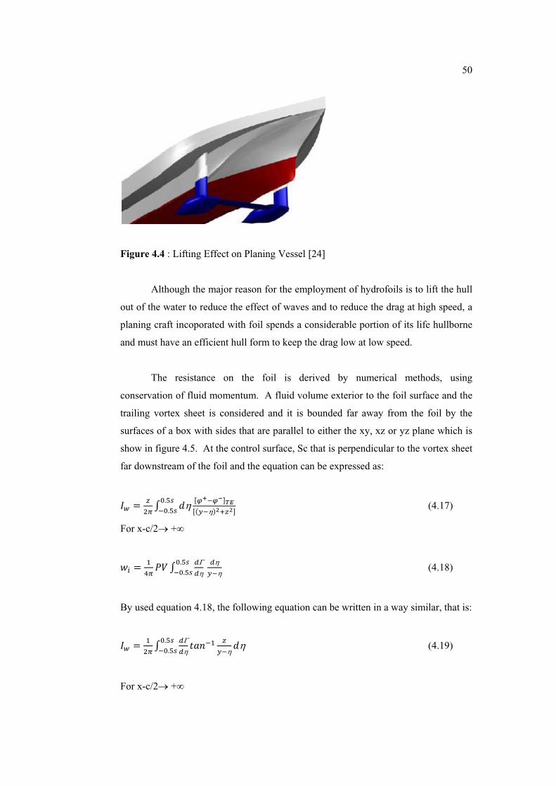
50

Figure 4.4 : Lifting Effect on Planing Vessel [24]

Although the major reason for the employment of hydrofoils is to lift the hull

out of the water to reduce the effect of waves and to reduce the drag at high speed, a

planing craft incoporated with foil spends a considerable portion of its life hullborne

and must have an efficient hull form to keep the drag low at low speed.

The resistance on the foil is derived by numerical methods, using

conservation of fluid momentum. A fluid volume exterior to the foil surface and the

trailing vortex sheet is considered and it is bounded far away from the foil by the

surfaces of a box with sides that are parallel to either the xy, xz or yz plane which is

show in figure 4.5. At the control surface, Sc that is perpendicular to the vortex sheet

far downstream of the foil and the equation can be expressed as:

�� A 6W" ¹ º�J>K!cJ>K! »¼½c¼�¾B¿»)Àc�+'e6'¾ (4.17)

For x-c/2� +�

�� A D " ÁX ¹ k�k�J>K!cJ>K! � k�Àc�

(4.18)

By used equation 4.18, the following equation can be written in a way similar, that is:

�� A DW" ¹ k�k�J>K!cJ>K! h5icD 6Àc�

º� (4.19)

For x-c/2� +�

51

The flow due to the vortex sheet is two dimensional in the yz plane at Sc

when the parameters � A )�c P �e+�>Â which means that the longitudinal velocity

is U at Sc. The momentum flux through the surface enclosing the control volume is

zero. The longitudinal pressure force acting on Sc:

TWÃ Ä��¼�À$W I ��¼

�6$WÅ º4º0&� (4.20)

Where � = �� . The additional longitudinal force acting on the control volume is the

force opposite the drag force D on the foil. This can be expressed as:

� A TWÃ Ä��¼�À$W I ��¼

�6$WÅ º4º0&� (4.21)

Figure 4.5 : The Drag Force on the Foil by using Conservation of Fluid

Momentum[34]

4.6 Resistance Components on the Foil and Strut

The resistance components in the planing craft condition for this study consist

of:

4.6.1 Viscous Resistance

The formulation of the viscous resistance coefficient on the foil and strut can

be expressed as:

52

�� A G��»F I G)hV8+ I QE)hV8+ ¾ (4.22)

Where:

�� A J>J�K)¦��#�fcW+' (4.23)

�� A ��

(4.24)

The viscous resistance can be calculated as follows:

�� A E>?��lXW( (4.25)

Where:

�� A Viscous resistance coefficient �� A Friction coefficient ��= Reynolds number

t/c =Foil thickness to chord ratio

V = Ship speed

c = Chord length

� = Kinematic viscosity

� = 1025 kg/m3

A = Planform area (the projected area of the foil in the direction of the lift force for

zero angle of attack). In the two dimensional, A is equal to the chord length c of the

foil.

In the two dimensional analysis, there are very small lift force occur which is

it can be assumed that the lift is nearly zero. Both foil and strut are using by similar

equation in order to predict the viscous resistance.

53

4.6.2 The Induced Resistance

The induced resistance due to the trailing vortex sheet of high aspect ratio

with zero camber and elliptical loading in infinite fluid were identified in this study.

This condition of foil and strut are going well with the Prandtl lifting theory which it

will derive the lift and resistance coefficient. Figure 4.6 show the flow is locally two

dimensional in the transverse cross sectional xz plane. Then it will give effect to the

vertical inflow velocity that changes the angle of attack of the incident flow.

Figure 4.6 : Steady Potential Flow Past a Two Dimensional Infinite fluid [34]

The induced resistance and lift force for foil and strut can be described as:

�� A E>?��lXW( (4.26)

�� A "ÆÇ)ÇeW+' (4.27)

�� A E>?��lXW( (4.28)

�� A È W"ÆWeHÇ'e (4.29)

Where: �� A Induced resistance coefficient �� A Lift coefficient

54

È A Aspect ratio, � !"�#$%= Angle of attack

V = Ship speed

c0 = Chord length at midspan

A = Planform area (projected area of the elliptical foil ,�&'Ç $)

s = Span length.

� = 1025 kg/m3

4.6.3 Wave Resistance

The wave resistance is caused by the lift and thickness of the foil or strut

itself. The wave resistance equation for vertical hull surface i.e. strut can be

expressed by Tuck Parabolic Strut [35] theory, as follows:

À� A W� ÉF P � _J>K�$WÊ (4.30)

When 4 < E

Then, the complex wave amplitude function ()*+ for waves with propagation

direction � can relate to the wave resistance by Newman [36] according to Michell

[37] thin ship theory. The equation ()*+ can be expressed as:

()*+ A W" Ë�p�8W*�Ì�Ã ÍÎÍ_ �ÏÐ!Ñ�'9)6e�_��!9+Ò (4.31)

By integrating equation 4.31 in the z direction, ()*+ can be expressed as:

()*+ A W" p�8�*� ¹ Ó_)\2 E+�VWÔ�VW ��!Ñ�9_�ÏF P �cÕ!Ñ�'9�Ò (4.32)

�� A DW xlXW ¹ Ö()*+ÖW×'c×' 8op*©�º* (4.33)

However, ()*+ in term of bF P �cÕ!Ñ�'9�d�in equation 4.32 is dependence on

the draft (D) of the strut (.i� A ��). When transverse waves correspond to smaller

55

� than the divergent waves, then bF P �cÕ!Ñ�'9�d A b�c!Ñ�'9V��Ød on .i� matters

for larger .i� for the transverse waves. According to equation (4.33), there has

connection between ()*+ and wave resistance, therefore this is relevant .i� on the

contribution from transverse and divergent waves to wave resistance. In that case, ()*+ is proportional to the B for a parabolic strut and gives result to the wave

resistance that proportional to B2. These mean that, the nondimensional wave

resistance can be expressed as:

��J>KT�'' (4.34)

Which is the nondimensional wave resistance not dependence on B but is a function

of�� and

��. Nevertheless, the nondimensional wave resistance will become

negligible or in other word very small effect to the wave resistance when�.i� A�H�� < =, based on the chord length c.

The wave resistance due to the foil also must be considered which is it gives

significant effect to the total resistance at high speed. The wave resistance due the

thickness and lift on a single foil can be illustrated as a thin flat foil at a submergence

h below the mean free surface. The linearized lift force can be expressed as:

� A PlX ¹ Ù)s+ºs�VWc�VW Ú PlXÛ (4.35)

The wave resistance dependence on the submergence Froude number of the

foil �).iÜ A ��Ü+ and the prediction of wave resistance based on a linear body

boundary condition and the linear free surface condition. Referring to Figure 4.7

gives illustration about the flow due to the foil by two vortices with opposite

circulation�Û. One vortex has a center in the foil at distance c/4 from the leading

edge and the other vortex has a center at the image point about the mean free surface.

The figure also explanation about velocity increases on the suction side of the foil

that result the circulation sign to the foil. Because the two vortices have opposite

signs i.e. Û, the rigid free surface condition is satisfied. According to the Weissinger

56

[38] approximation, the boundary condition has to satisfy only at one point, at

distance ¾ from the leading edge. The image vortex effectively causes an increase in

the angle of attack at this point. This means a higher lift coefficient, CLw value and

also the closer image vortex that increase the CLw value.

Figure 4.7 : The Flow due to the Foil By Two Vortices with Opposite Circulation�Û[34]

The circulation�Û of the foil can be calculated as follow:

Ý"� P J>K�ÝW") Ü'eJ>WK�'+ A X �% I Wm� $ (4.36)

Then the lift on the foil can be evaluated by using the Kutta-Joukowski formula

below.

�� A PlXÛ (4.37)

and lift coefficient can be expressed as: �� A ��J>KT�'� (4.38)

The wave resistance due to the foil can be described as:

�� A T�Ý'�' ��Þ �'´fß'à (4.39)

and the wave resistance coefficient can be expressed as:

57

�� A ��J>KT�'� (4.40)

Where: �� A Wave resistance coefficient �� A Lift coefficient , A Maximum camber %= Angle of attack (deg)

V = Ship speed

c = Chord length

� = 1025 kg/m3

4.6.4 Spray Resistance

This situation is arising when the Froude number is larger approximately than

0.5 which the occurrence of the spray increases with the speed. The spray resistance

is caused both by potential flow and viscous flow effect. Hoerner [39] simply set the

spray resistance as follow:

�! A E>FGlXWhW (4.41)

This equation is valid when the Froude number based on the chord length�).i� A�H��+ < =. Where V is ship speed and t is thickness of the foil or strut.

4.7 The Combination Total Resistance

The total resistance for the vessel on planing hull taking account from

resistance on barehull and the foil and strut. In this prediction of resistance, different

methods are use in order to calculate the resistance. Savitsky method is use for

prediction resistance of barehull while numerical method in two dimensional is use

58

for predict the resistance of foil and strut. The sample calculation of resistance

prediction for model with stern foil is shown in Appendix C.

The formulation of total resistance can be expressed as:

RT= Rbarehull (vessel)+(Rv+Ri+Rw+Rs)foil+(Rv+Ri+Rw+Rs)strut (4.42)

4.8 Sinkage and Trim

The hydrodynamic force put forth on ship’s hull due to its forward motion

causes forces which are capable of altering the attitude of the ship, inducing both a

vertical movement or ‘sinkage’ (positive downward) and a rotation or ‘trim’ angle

(positive when bow up). The combination of these two quantities is referred to as

‘squat’.

Squat phenomenon is small for displacement vessels but it effect to small

craft especially at high speed craft, involving vertical displacements of only at most a

few percent of the vessel’s draught at most speeds. Sinkage is generally positive at

normal speeds, i.e. the ship’s effective draught is increased. The positive sinkage

reaches a maximum at Froude numbers of the order of 0.5, the reduction and may go

negative at very high speeds, although the latter phenomenon has seldom being

investigated for displacement vessels. However, at high speeds there is a connection

between the squat phenomenon and the mechanism of planing, as a negative sinkage

or rise in the water is induced by positive hydrodynamic lift. In that case however,

for vessels capable of planing, the magnitude of squat is no longer small relative to

the draught.

59

4.9 Program Development of Resistance Prediction

Basically computer programming is able to calculate the mathematical

formulation when input data are specified by the user. In this case, by using

FORTRAN (Formula Translation) program the resistance prediction can easily

determine by specifying the formulation. In order to run the FORTRAN programme,

it may have the source code to carry out this calculation. Before that, this program

may require the input data of vessel. The input data are saved into notepad file q.text

and the input data contain of ship particular and foil strut parameters that have

written in the program.

Basically the formula that used in the program resistance prediction for

barehull is Savitsky Method and while for stern foil is 2D Method. The detail

formulation of this program please refers to section 4.3 and 4.6 of this chapter. The

result of calculation in this program was saved into output.txt. The source code,

input and output data as illustrate in Appendix D.


The resistance of the ship is able to predict by right method which must be

decided at preliminary design stage. If incorrect or wrong method was selection then

it will result the unenthusiastic answer either it give underestimate or overestimate

calculation. In this case, the prediction performance using Savitsky method and 2D

methods are used in order to calculate the resistance of the ship incorporating with

stern foil.

CHAPTER 5

SEAWORTHINESS

5.1 Introduction

In the operation and design of high speed crafts, seakeeping performance is

an important task because it has been proven that large motions and accelerations can

degrade the operational capabilities of the ship. The high speed craft especially

planing hull, sometimes exhibit an effect such as deck wetness, slamming and loss

speed caused by the couple of heave and pitch. The vertical motions of high speed

craft have negative consequences that limit the speed. It is not only a matter of

structural damage or safety risks. When the frequencies of vertical motions are

around 1 rad/sec effect by couple heave and pitch motion, they contribute in a

cumulative way to sea-sickness of the crew.

From these research projects it became evident that the behavior of high

speed craft in waves was strongly nonlinear by nature. This makes applying normal

ship motion calculation routines and analysis procedures limited applicable. Also the

limiting criteria for establishing the operability of these fast craft were found to be

vastly different from those used for low speed displacement ships. From full scale

observations it was evident the most of the speed reduction applied in fast craft

operations in waves was voluntary. In order to improve the seaworthiness of the

vessel, by it mean the vessel are able to move at maximum speed in rough condition,

there are required equipment for reducing these motion. But this is much more

difficult than for reducing roll because of the large pitching inertia moment of the

vessel.

61�

Various methods have been used to improve the seaworthiness of a boat, such

as changing the main dimensions, choosing the type of lines and changing the

distributing of weight. But the most effective way is by using a stabilizer. Recently

stabilizing fins have been used to reduce roll. Heaving and pitching of boats brings

on a series of effects, such as seasickness, deck wetness, slamming and speed loss.

In order to reduce these effects, equipment for effectively reducing pitching is

needed. But this is much more difficult than that for reducing roll, because of the

very large pitching inertia moment of the boat. For a high speed planing boat, the

pitching moment is relatively smaller, and a high speed moving hull can supply large

dynamic forces, so it should be possible to install equipment for reducing pitch.

The improvement of seaworthiness in planing craft was studies by numerous

researchers in reducing the motion. However, Savitsky and Brown (1976) [33] were

initially derived the formulation for reducing the motion in heave and pitch at high

speed by using wedge or flap in their experiment i.e. empirical method. In 1985,

Long Wen [22] was performed tests with the planing craft model with transom flap

for improved seakeeping ability for a single boat with a load coefficient of 0.54 over

a range of speed coefficient from one to three. Other test he performed includes

measuring the steady state normal force and hinge moment of tansom flaps. In his

research used the model without flap and with 12.5% flaps (flaps length or chord

equal to 12.5%of the beam) with an angle of 0o and 3o, frequency response plot for

the vessel on smooth water with oscillating flaps.

Unfortunately the hull form which Long Wen used was not a simple prismatic

hull and the speed range used is on the low side for the equation used in developing

the theoretical model. Figure 5.1 shows the hull model which Long Wen used in

performing his test and figure 5.2 is the prismatic hull form which used for

theoretical calculations. Long Wen’s model has varying deadrise angles in front of

40% of the length, keel line curvature in front of 40% and varying beam along the

complete length. The beam of Long Wen’s model was 0.37m, the length was 1.5m

and the mass was 27.3kg. For prismatic model used in calculations has constant

beam equal to the mean beam of Long Wen’s model and constant deadrise angle of

24o as the same as that for the last 60% of Long Wen’s model.

62�

Figure 5.1 : Long Wen’s Experiment Model [22]

Figure 5.2 : Prismatic Hull Model [22]

In this research, the foil with strut is used in order to search out better

seaworthiness especially for high speed craft (M Hull). Basically the idea of

installation is obtain from hydrofoil vessel which it resulting positive in term of

seakeeping performance. The advantageous of this foil or so called stern foil it able

to minimize the vertical motion of heave and pitch that will be maintained the speed.

The ship in this research basically has its own direction of motion which has

six degrees of freedom (6 D.O.F) and these motions are classified as movements of

the centre of gravity. The motions of ship could be divided into two categories that

a

D

F

M

T

R

t

m

c

e

p

are translatio

D.O.F) whil

Figure 5.3 :

Movements

Translationa

Rotational

The r

trim. Whil

moment or

constant as l

Evalu

environment

principal rea

onal and rota

e table 5.1 d

Types of Sh

Table 5

al

Surge

Sway

Heav

Roll a

Pitch

Yaw

roll and pitc

e in transla

force genera

long the ship

uation of a

tal condition

ason why an

ational. Figu

describes ship

hip Motions

5.1 : Ship’s S

e in the x dir

y in the y dir

ve in the dire

about x axis

about y axi

about z axis

ch motion of

ational and r

ates for swa

p is in neutra

vessel’s sea

ns (wave sp

ny comparis

ure 5.3 show

p motions te

[40]

Six Degree o

D

rection of sh

ection of shi

ction z axis

and makes t

is which cau

s and the mo

f ship are ha

rotational m

ay, surge an

al equilibrium

akeeping per

pectra) and

on for altern

ws the compl

erm [40].

of Freedom (

Description

ip and acts f

ip and move

and moving

the starboard

uses the bow

vements of s

aving dynam

motion, there

nd yaw, prov

m condition.

rformance d

the defined

native vesse

lete set of sh

(6 D.O.F)

forward

e towards sta

g downwards

d side up and

up

ship is bow t

mic equivalen

e would be

vided the di

depends hea

d criteria, an

l speeds, inc

6

hip motions

arboard

s

d down

to starboard

nt of heel an

no residua

isplacement

avily upon th

nd this is th

cident wave

63�

(6

nd

ary

is

he

he

e a

64�

heading, loading conditions, etc is a complex matter. Seakeeping analysis is

essentially a three part problem:

1. Estimation of the likely environmental conditions encountered by the vessel,

based on hindcast or predicted weather data as applicable (e.g. wind, wind wave,

swell).

2. Determination of the vessel’s response characteristics (response amplitude

operator, RAO).

3. Specification of the criteria being used to assess seakeeping behaviour (e.g.

cargo acceleration, deck wetness, motions sickness).

Head sea waves are considered in this research which the RAO of heave

refers to steady-state amplitude of heave divided by the incident wave amplitude in

regular incident waves. Similarly, the RAO of pitch it refer to mean amplitude of

pitch divided by the wave slope multiply with waves amplitude or regular waves.

5.2 Regular Waves

The regular waves or irregular waves are proportionally caused by wind with

various speeds at sea surface. By right, the waves that always hit or cross the ship

are considered as irregular waves and no regular waves could be generated at sea

naturally. The waves that generally effect the ships characteristic might be in

irregular waves or sometime in random.

The regular waves could not be generated in sea or ocean but this type of

waves is taking into account during the seakeeping assessment. Most preferably this

wave is known as an ideal. This ideal wave mentioned above is possible to be

generated using towing tank facilities in laboratory. The experimental methods could

be used to analyze ship model on seakeeping assessment. Other than this, there is

another important fact by assumption where the theory of irregular waves can be

65�

represented by superimposing or adding together a suitable assembly of regular

waves.

The regular wave condition can be concluded that the characteristics of a ship

at rough weather conditions could be determined by just referring to the regular

waves criterion. The conditions or results are still acceptable although the ship does

not encounter or face real situations at the sea. Therefore, an understanding of the

theory and nature becomes important criteria to conduct seakeeping studies on any

particular ships. An image of regular waves generated using towing tank facilities in

laboratory is illustrated in figure 5.4. The waves are in two-dimensional and they

travel ahead in x direction while the crests are 90 � to x – axis [41].

Figure 5.4 : Regular Waves Generated in Towing Tank [41]

5.3 Motion in Regular Waves

5.3.1 Lateral Plane Motion in Regular Beam Seas

The roll motion of a ship occurs when the starboard side is exposed to the

regular (model test condition) or irregular (real sea condition) waves at beam angle

90�. Roll motion of a ship occurs about the x direction by rotation at starboard or

66�

portside. Thus, the clear illustration is in figure 5.3. At this moment, the waves will

be having resultant force and the force acting on a particle in the wave surface

remains equal to the wave surface. In the case of wave length longer than the beam

of ship, it is reasonable to assume that the ship is acted by a resultant force normal to

an ‘effective wave surface’ which takes into account all the sub – surfaces interacting

with the ship.

By the assumption made by R.E .Froude, the effective wave slope is

subsurface occurs at the centre of buoyancy when rolls. Then, the general equation

of motion for rolling in waves becomes [40]. However in this study only emphases

on the vertical plane such as pitch and heave which gives much impact on high speed

condition especially on planing craft (M Hull).

5.3.2 Vertical Plane Motion in Regular Head Waves [42]

Ship motion in regular head seas contributes motions such as heave, pitching

and surge. At this stage, roll, yaw and sway are in the neutral condition and these

three motions could not be analyzed. At the event of long waves, the encounter

frequency, �e seems to be very low and at this moment, dynamic effects, added mass,

and damping are virtually negligible. Thus, excitation of the ship is fully influenced

by the buoyancy changes, provided the long waves. Figure 5.4 shows the maximum

heave and pitch during the event in long waves [43]

In short waves, the excitation is not very significant and this occurs because

in short waves, the buoyancy forces assist together with the ship hull. Here, it can be

concluded that ships having significant excitation if the wave’s length is about three

quarter of ship length.

5.4 Couple Heave and Pitch Motion in Head Sea

As described earlier, the pitch motion of a ship in the waves act in rotational

motion about y - direction as shown in figure 5.3. It is always concentrates on head

67�

seas where the heading angle will be 180 � opposing the waves. The pitch motion

normally having an encounter frequency due to its direction touches the successive

wave crests [43]. The heave motion in regular waves is considered as movement of

ship in vertical plane motion and the motion acts transitional. Since its buoyant force

is then greater than its weight, the ship will move vertically up. Whilst the

equilibrium is reached, the ship continue rising because of its momentum. Then the

weight is greater than the buoyant force and it will tend to slow the motion. The

process of a ship move vertically up and down will be continue indefinitely if there is

no damping force acts in the opposite direction of motion and this known as a

heaving. This condition occurs when the ship reach at extreme position at velocity is

finally zero and the ship will move vertically downward since the weight is greater

than buoyant force.

This couple of motion was dealing with vertical motion which can be

investigated in a model basin. Actually the coupled heave and pitch for the head sea

condition also can be investigated analytically by the strip theory method. Basically

the strip theory was derived two equations for heave and pitch respectively.

According to Newton’s second law, at any instant all vertical forces on the ship are in

dynamic equilibrium. Thus, the heaving and pitching equation can express as:

j01 -.� (5.1)

�*1 A -/ (5.2)

Where -. = The sum of various fluid forces (vertical hydrodynamic forces as well as the

wave excitation force)

-/ = The sum of corresponding moments acting on the vessel because of relative

motion of vessel and wave.

68�

5.4.1 Basic Concept of Couple Heave and Pitch Motion

In order to simplified this complex motion problem several assumptions and

limitations have been made as follows:

1. The ship must be heading into the waves in a direction transverse to their

crest line.

2. The seaway is considered to consist of regular harmonic waves.

3. The ship motions of surge, sway, yaw and roll are neglected.

Korvin-Kroukovsky [44] approach was to consider a ship hull as a series of

transverse segment or strip and to treat the flow adjacent to each as two dimensional

in nature. The effect was to reduce the problem from three to two dimensions with

each strip assumed to be a part of an infinite cylinder having two dimensional around

it. The vertical motion of each strip is assumed to be composed of the combined

pitching and heaving motions. When the response of each strip calculated, the total

ship response can be found by integrating the component reactions of all the strips

along the ship’s length. The basic mathematical equation obtained in this way is a

linear second order differential equation describing the inertial, hydrodynamic and

hydrostatic components of force acting on each strip and caused by relative vertical

motion between the ship and the wave.

The general equation coupled of heaving and pitching can be expressed as:

É�n I 566Ê 01 I 76603 I 8660 I 569*1 I 769*3 I 869* A .)]+ )�99 I 599+*1 I 799*3 I 899* I 59601 I 79603 I 8960 A /)]+ (5.3)

Which each term represents the moment of force instead of the force.

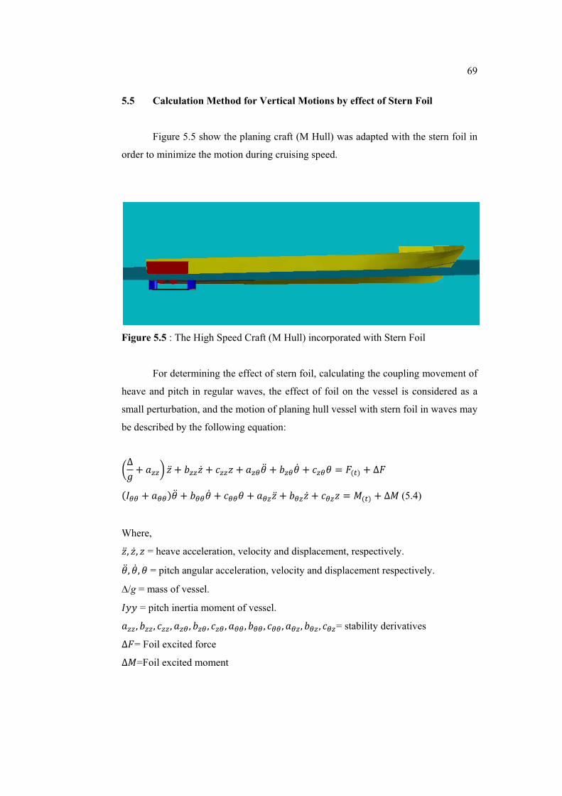
69�

5.5 Calculation Method for Vertical Motions by effect of Stern Foil

Figure 5.5 show the planing craft (M Hull) was adapted with the stern foil in

order to minimize the motion during cruising speed.

Figure 5.5 : The High Speed Craft (M Hull) incorporated with Stern Foil

For determining the effect of stern foil, calculating the coupling movement of

heave and pitch in regular waves, the effect of foil on the vessel is considered as a

small perturbation, and the motion of planing hull vessel with stern foil in waves may

be described by the following equation:

É�n I 566Ê 01 I 76603 I 8660 I 569*1 I 769*3 I 869* A .)]+ I �.

)�99 I 599+*1 I 799*3 I 899* I 59601 I 79603 I 8960 A /)]+ I �/ (5.4)

Where, 012 032 0 = heave acceleration, velocity and displacement, respectively. *1 2 *3 2 * = pitch angular acceleration, velocity and displacement respectively.

�/g = mass of vessel. �44 = pitch inertia moment of vessel. 5662 7662 8662 5692 7692 8692 5992 7992 8992 5962 7962 896= stability derivatives �.= Foil excited force �/=Foil excited moment

70�

In this study, the calculation used is strip theory method for the hull dynamics

and for estimating the values of ��. and �/ or calculating the stern foil by using

Savitsky and Brown’s empirical plus two dimensional methods. The equation for

calculating forces and moments of stern foil by using empirical method will be added

to the dynamics equation in order to suit the characteristic and study objectives. The

selection of stern foil parameter has been decided according to is resistance

increament due to the seakeeping performance. The parameters of the stern foil was

designed will be described in Chapter IV.

5.5.1 Exciting Forces and Moments due to Stern Foil for Planing Hull

The total lift force can be expressed as:

��] A �� I �� I �� (5.5)

The equation for lift force due to viscous drag as follows:

�� A E>?��lXW( (5.6)

�� A Gx)% P %J) (5.7)

Where: �� A Lift coefficient due to Viscous %��= Angle of attack in radian

V = Ship speed %0 = Uncamber foil and zero flap=0

A = Chord length (c)

� = 1025 kg/m3

While for lift force due to induced drag can be expressed as:

�� A E>?��lXW( (5.8)

71�

�� A È W"ÆWeHÇ'e (5.9)

Where:

�� A Lift coefficient due to Induced Drag È A Aspect ratio, � !"�#$ %= Angle of attack

V = Ship speed

c0 = Chord length at midspan

A = Planform area (projected area of the elliptical foil ,�&'Ç $)

s = Span length.

� = 1025 kg/m3

Then the lift force due to wave resistance can be described as:

Ý"� P J>K�ÝW") Ü'eJ>WK�'+ A X �% I Wm� $ (5.10)

�� A PlXÛ (5.11)

and lift coefficient can be expressed as: �� A ��J>KT�'� (5.12)

According to large aspect-radio theory of wing in figure 5.6, the lift of a stern

foil on planing craft is:

Figure 5.6 : Theory of Wing

72�

The detailed expression of lift can be obtained as follows:

�. A �� I �� I �� (5.13)

In this equation the moment about the center of gravity is,

�/� A �.á[ (5.14)

Where effective length á[ of stern foil to center of gravity as shows in figure 5.7 can

be expressed as follows:

á[ A D 8 I â�ek¶ã�[ �� (5.15)

Figure 5.7 : Effective Length of Stern Foil

5.5.2 Solution of the Motion Equation with Stern Foil

Substituting equation (5.13) and equation (5.14) into equation (5.16) the

motion of planing craft with stern foil in waves may be described by the following

equation:

É�n I 566Ê 01 I 76603 I 8660 I 569*1 I 769*3 I 869* I �. A .)]+ )�99 I 599+*1 I 799*3 I 899* I 59601 I 79603 I 8960 I �.á[ A /)]+ (5.16)

73�

In its simplest form, the vessel may be considered like an electronic filter. It

takes an input signal (the ocean waves), filters it, and the produces an output (the

vessel motions). In most cases, this simple method is quite valid and produces useful

results. The vessel’s filter function which is also named Response Amplitude

Operators (RAO) are different for the six, rigid-body degrees freedom of ship

motions. Each motion has its own characteristics and RAO.

RAO are derived from the amplitudes by dividing the motion response by the

wave input parameter:

äåæ A çèéêèë�äìíîèëíìïðñì�òëîóé�ôðõðöìéìõí The RAO for pitching and heaving are defined as below:

Pitching RAO = Pitch Amplitude / Wave Slope

a

a

k��

�

Heave RAO = Heave Amplitude / Wave Amplitude

a

az

��

5.6 SEAKEEPER Program [26]

SEAKEEPER is the seakeeping analysis program in the Maxsurf software

package. It uses the Maxsurf geometry file to calculate the response of the vessel to

user-defined sea conditions. In order to calculate the vessel response, linear strip

theory based on the work of Salvesen et al (1970), is used to calculate the coupled

heave and pitch response of the vessel. The roll response is calculated using linear

roll damping theory. In addition to graphical and tabular output of numerical results

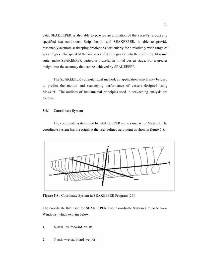
d

s

r

v

s

i

t

M

f

5

c

F

T

W

2

data, SEAK

specified se

reasonably a

vessel types

suite, make

insight into t

The

to predict t

Maxsurf. T

follows:

5.6.1 Coor

The c

coordinate sy

Figure 5.8 :

The coordin

Windows, w

1. X-ax

2. Y-ax

KEEPER is a

ea condition

accurate seak

. The speed

SEAKEEPE

the accuracy

SEAKEEPE

the motion

The outlines

rdinate Syst

coordinate s

ystem has th

Coordinate

nate that used

which explain

xis +ve forwa

xis +ve starb

also able to p

ns. Strip th

keeping pred

of the analy

ER particula

y that can be

ER computat

and seake

of fundam

tem

system used

he origin at t

System in S

d for SEAK

n below:

ard -ve aft

oard -ve por

provide an a

heory, and

dictions part

ysis and its in

arly useful i

achieved by

tional metho

eeping perfo

ental princip

by SEAKEE

the user defin

SEAKEEPER

KEEPER Use

rt

animation o

SEAKEEP

ticularly for

ntegration in

in initial de

y SEAKEEP

od, an applic

ormance of

ples used in

EPER is the

ned zero poi

R Program [

er Coordinat

f the vessel

ER, is abl

a relatively

nto the rest o

esign stage.

PER.

cation which

f vessels de

n seakeeping

same as for

int as show i

26]

te System si

7

’s response

e to provid

wide range

of the Maxsu

For a great

h may be use

esigned usin

g analysis a

Maxsurf. Th

in figure 5.8

imilar to vie

74�

to

de

of

urf

ter

ed

ng

are

he

.

ew

3

a

o

p

d

(

a

o

p

F

s

s

5

d

O

i

3. Z-ax

Whe

about the cen

of gravity i

positions are

degrees of f

(linear moti

about the x,

often given

pitch 5.

Figure 5.9 :

Wav

symbol �. T

seas 180° an

5.6.2

Irreg

describes the

Ocean wave

irregular wav

is +ve up -v

n calculating

ntre of gravi

s of interest

e measured

freedom, thr

ons in x, y,

, y, z axes r

the subscrip

Wave Direc

e direction

Thus followi

nd port beam

Wave Sp

gular ocean

e distributio

es are often c

ves.

e down

g motions at

ity. Hence t

t. SEAKEE

in the coord

ree linear an

, z axes resp

respectively)

pts 1 to 6; t

ctions in SEA

is measured

ing waves a

m seas 270° a

pectra

waves are

on of wave e

characterised

t remote loc

the distance o

EPER calcu

dinate system

nd three ang

pectively) a

). For conv

thus heave m

AKEEPER S

d relative to

are at � = 0°

as shown in f

often charac

energy (heig

d by statistic

ations, the v

of the remot

ulates this d

m described

gular. These

and roll, pitc

venience, the

motion woul

System [26]

o the vesse

°; starboard

figure 5.9.

cterised by

ght) with fre

cal analysis

vessel is assu

te location fr

istance inter

above. A v

e are: surge

ch, yaw (ang

e degrees of

ld have a su

el track and

beam seas

a "wave sp

quency. Ch

of the time

7

umed to rota

rom the cent

rnally and a

vessel has s

, sway, heav

gular motion

f freedom a

ubscript 3 an

d is given th

are 90°; hea

pectrum", th

haracterisatio

history of th

75�

ate

tre

all

six

ve

ns

are

nd

he

ad

his

on

he

76�

Irregular ocean waves are typically described in terms of a wave spectrum.

This describes a wave energy distribution as a function of wave frequency. The

continuous frequency domain representation shows the power density variation of the

waves with frequency and is known as the wave amplitude energy density spectrum,

or more commonly referred to as the wave energy spectrum. The spectral ordinates

(or wave spectral density) are given the symbol: S�(). (This is similar to the power

spectral density, PSD, used in electronics and communications analysis.) A typical

wave spectrum is shown in figure 5.10 below:

Figure 5.10 : Typical Wave Spectrums [26]

5.6.3 Idealised Spectra

It is often useful to define idealised wave spectra which broadly represent the

characteristics of real wave energy spectra. Several such idealised spectra are

available in SEAKEEPER and are described below:

1. Bretschneider or ITTC two parameter spectrum.

2. One parameter Bretschneider.

3. JONSWAP.

4. DNV Spectrum.

5. Pierson Moskowitz.

77�

5.6.4 Encounter Spectrum

An important concept when calculating vessel motions is that of the

encountered wave spectrum. This is a transformation of the wave spectrum which

describes the waves encountered by a vessel travelling through the ocean at a certain

speed. This is effectively a Doppler shift of the spectrum which smears the spectrum

towards the higher frequencies in head seas and towards the lower frequency in

following seas.

5.6.5 Characterising Vessel Response

This section outlines the method used to describe a vessel's response in a

seaway. Harmonic Response of Damped, Spring, Mass system for most purposes, it

is sufficient to model the vessel as a set of coupled spring, mass, damper systems

undergoing simple harmonic motion. This is assumed by SEAKEEPER and most

other seakeeping prediction methods. This method may be successfully applied to

the analysis of the vessel's motions provided that these motions are linear and that the

principle of superposition holds. These assumptions are valid provided that the

vessel is not experiencing extremely severe conditions.

5.6.6 Response Amplitude Operator (RAO)

The Response Amplitude Operator (RAO), also referred to as a transfer

function (this is similar to the response curve of an electronic filter), describes how

the response of the vessel varies with frequency. These are normally non-

dimensionalised with wave height or wave slope. Typical heave and pitch RAOs are

shown in figure 5.11 below:

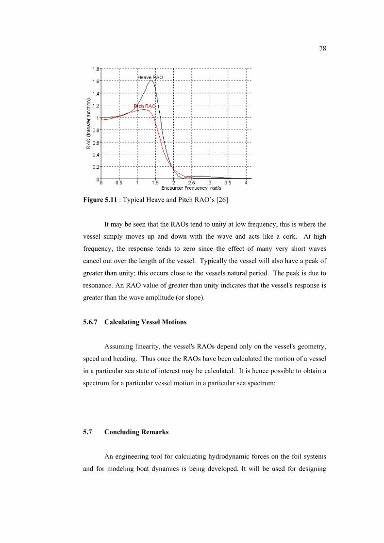
78�

Figure 5.11 : Typical Heave and Pitch RAO’s [26]

It may be seen that the RAOs tend to unity at low frequency, this is where the

vessel simply moves up and down with the wave and acts like a cork. At high

frequency, the response tends to zero since the effect of many very short waves

cancel out over the length of the vessel. Typically the vessel will also have a peak of

greater than unity; this occurs close to the vessels natural period. The peak is due to

resonance. An RAO value of greater than unity indicates that the vessel's response is

greater than the wave amplitude (or slope).

5.6.7 Calculating Vessel Motions

Assuming linearity, the vessel's RAOs depend only on the vessel's geometry,

speed and heading. Thus once the RAOs have been calculated the motion of a vessel

in a particular sea state of interest may be calculated. It is hence possible to obtain a

spectrum for a particular vessel motion in a particular sea spectrum:


An engineering tool for calculating hydrodynamic forces on the foil systems

and for modeling boat dynamics is being developed. It will be used for designing

79�

hydrofoil-assisted craft, which SEAKEEPER is used in this study. This relatively

simple approach is suitable for parametric studies of the influence of foil elements on

hydrodynamic seakeeping performance. Stern foil sections that improve boat

performance will also be incorporated into the tool. Planing hull elements will be

added to model transitional regimes of pure hydrofoil boats and service regimes of

hydrofoil assisted ships. The theoretical in seakeeping also important in order to

cross check the seakeeping prediction.

CHAPTER 6

RESEARCH OBJECT

6.1 Introduction

The research to be done is intended on the resistance and seakeeping test and

is conducted in the Marine Technology Laboratory, Universiti Teknologi Malaysia.

In this case, the research will be conducted on resistance in calm water and

seakeeping test for planing craft at speed 25 knots with and without stern foil in

regular waves. As previously stated these models are based on full sized ships.

When expanding the model results to full scale, full scale use was made of the ITTC

57 friction line as well as applying a ship-model correlation allowance of 0.0006981.

A summary of the ship and model including stern foil parameters features are shown

below in table 6.1 and table 6.2. This craft was designed for high speed i.e. 25 knot at

maximum continuous speed. The body plan with and without stern foils of the vessel

are shown in figure 6.1 and figure 6.2 respectively. The offset data of vessel is shown

in Appendix E. Figure 6.3 and 6.4 shows the resistance tests which were conducted

for both conditions with and without stern foil at various speeds.

Seakeeping test is meant to measure the behaviour of the vessel at seas.

Model testing provides an attractive alternative. The seakeeping test can predict the

characteristics of the vessel in term of motion which is it gives significant effect on

itdynamics stability. The success of a ship design depends ultimately on its

performance in a seaway. However, in a realistic seaway it is such a complex

problem that ship designers are generally forced to select their hull forms and ship

81��

��

dimensions on the basis of calm water performance without much consideration of

the sea and the weather conditions. Figure 6.5 and 6.6 show seakeeping test which

was conducted according to the test protocol in order to determine the RAO for

heave and pitch.

Table 6.1 : Main Particular of Planing Craft (M Hull)

Parameters Ship Model

Length overall LOA 34 2.194

Length of waterline LWL (m) 31.667 2.043

Waterline beam (m) 7.4167 0.4785

Design Draught T(m) 1.365 0.0881

Depth (m) 3.300 0.2129

Deadrise angle � (deg) 14 14

Midship area coefficient, Cm 0.695 0.695

Block coefficient, Cb 0.46 0.46

Waterplane area coefficient, Cwp 0.817 0.817

Wetted Surface Area (m2) 220.000 0.9157

Displacement, � (Tonne) 130.275 0.0341

LCG from Midship (m) -2.258 -0.1457

VCG from keel (m) 2.124 0.1370

Linear scale ratio, 1:15.5

Table 6.2 : Stern Foil Parameters

Model Prototype

Foil

Height (h) m 0.071 1.1005

Chord Length (c )m 0.065 1.0000

Span (s) m 0.452 7.0000

Thickness (t) m 0.008 0.1194

Angle of Attack deg 0.000 0.0000

Camber (f) 0.000 0.0000

�

F

F

Strut

Height (h) m

Chord Leng

Thickness (

Angle of A

Camber (f)

Figure 6.1 :

Figure 6.2 :

m

gth (c )m

(t) m

ttack deg

Body Plan o

Body Plan o

Model

0.071

0.021

0.006

0.000

0.000

of Planing C

of Planing C

Pr

1.

0.

0.

0.

0.

Craft (M Hul

Craft (M Hul

rototype

1005

3255

0930

0000

0000

ll) without S

ll) with Stern

tern Foil

n Foil

882�

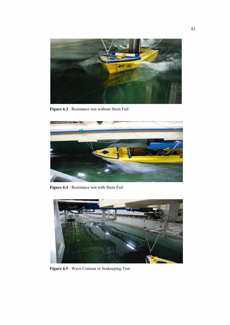
83��

��

Figure 6.3 : Resistance test without Stern Foil

Figure 6.4 : Resistance test with Stern Foil

Figure 6.5 : Wave Contour in Seakeeping Test

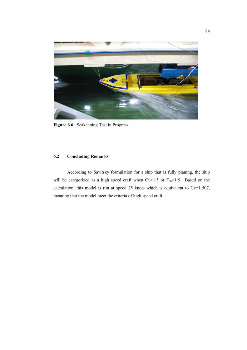
84��

��

Figure 6.6 : Seakeeping Test in Progress


According to Savitsky formulation for a ship that is fully planing, the ship

will be categorized as a high speed craft when Cv>1.5 or Fnb>1.5. Based on the

calculation, this model is run at speed 25 knots which is equivalent to Cv=1.507,

meaning that the model meet the criteria of high speed craft.

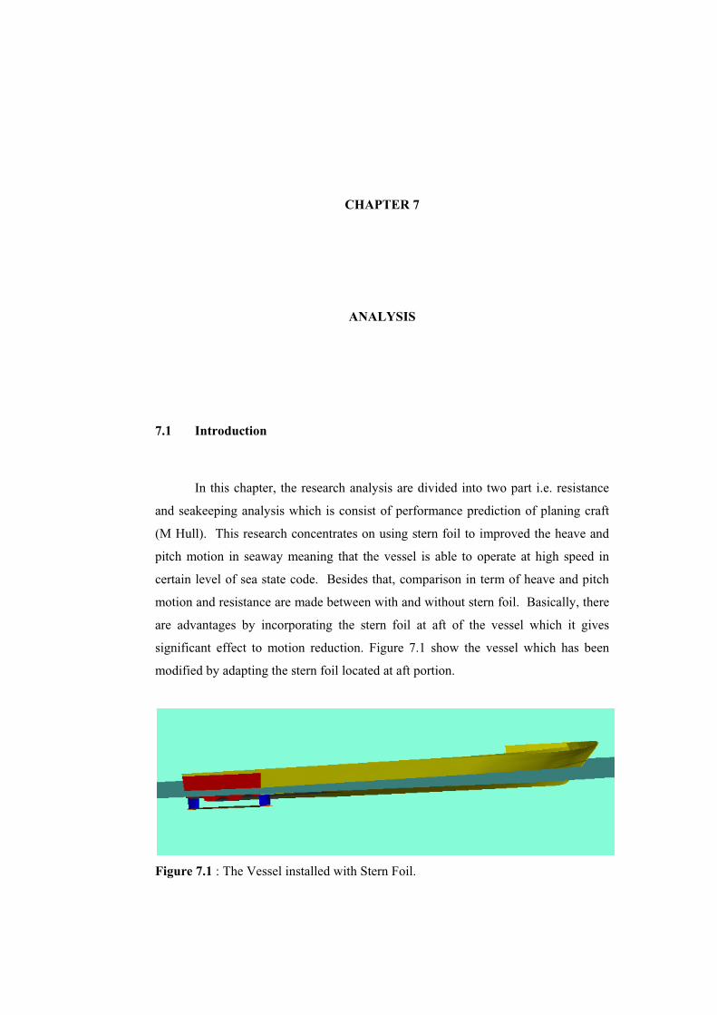
CHAPTER 7

ANALYSIS

7.1 Introduction

In this chapter, the research analysis are divided into two part i.e. resistance

and seakeeping analysis which is consist of performance prediction of planing craft

(M Hull). This research concentrates on using stern foil to improved the heave and

pitch motion in seaway meaning that the vessel is able to operate at high speed in

certain level of sea state code. Besides that, comparison in term of heave and pitch

motion and resistance are made between with and without stern foil. Basically, there

are advantages by incorporating the stern foil at aft of the vessel which it gives

significant effect to motion reduction. Figure 7.1 show the vessel which has been

modified by adapting the stern foil located at aft portion.

Figure 7.1 : The Vessel installed with Stern Foil.

86��

7.2 Resistance Analysis

An example of resistance calculation using Savitsky Method and 2D

formulations are shown in Appendix C. While the source code and input data for

calculation using FORTRAN program is shown in Appendix D which consist of

input data, source code and output data. In order to validate the resistance prediction,

the resistance test was conducted for both models (with and without stern foil) where

the comparisons can determine either the formula are appropriate or not.

Table 7.1 and figure 7.2 shows the comparison between theoretical and

experimental resistance result for a ship without incorporating stern foil at calm

water condition. From the result it show that the variance of resistance values

between theory and experiment. The variance resistance value between both

methods is 37.89%, at speed 23 knots which is calculation using theoretical (Savitsky

Method) resulting high value compare to the resistance value that was carryout by

experiment. However, this value is large due to linearized formulation by Savitsky

equation. At speed 26 knots the variance of resistance between both methods are

15.62%, where the result of resistance test from experiment closely agreed to the

resistance value obtained by theory (Savitsky Method). The theory prediction

resulting better performance at speed 28 knots where the discrepancy value is 5.32%.

Table 7.1 : Resistance Result for a ship without Stern Foil

Resistance (N)

Vs(knots) Theoretical Experiment

23 95346.63 59244.09

24 99696.57 66787.36

25 104081.14 77299.11

26 108480.54 91535.98

28 117240.33 123473.10

30 125808.06 141895.51

87��

Figure 7.2 : Graphs on Comparison between Theory and Experiment for Resistance

without Stern Foil

From table 7.2 and figure 7.3 shows the resistance value for both theoretical

and experiment methods for a ship incorporating with stern foil at 0o degree angle of

attack. The result between theoretical and experiment resulting small variance where

the percentage ranges for every speed are at 7-20%. From this table and graph the

resistance values are slightly higher when compare to theoretical prediction.

Table 7.2 : Resistance Result for a ship with Stern Foil (0o)

Resistance (N)

Vs(knots) Theoretical (N) Experiment (N)

23 97063.33 104980

24 101556.01 110070

25 106088.69 125860

26 110641.57 140620

28 119724.28 144670

30 128636.11 154240

0.00E+00

2.00E+04

4.00E+04

6.00E+04

8.00E+04

1.00E+05

1.20E+05

1.40E+05

1.60E+05

20 22 24 26 28 30 32 34

Resistan

ce�(N

)

Speed�(Knots)

Resistance��Without�Stern�Foil

(Theory)

(Exp)

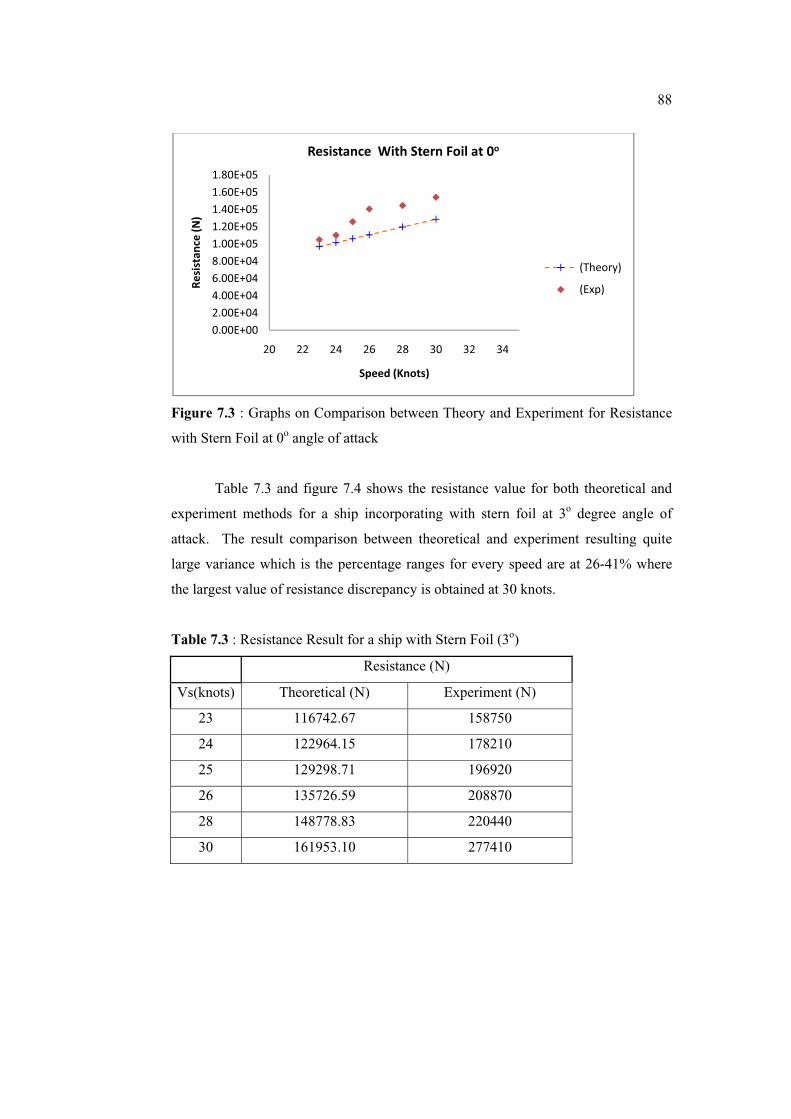
88��


with Stern Foil at 0o angle of attack

Table 7.3 and figure 7.4 shows the resistance value for both theoretical and

experiment methods for a ship incorporating with stern foil at 3o degree angle of

attack. The result comparison between theoretical and experiment resulting quite

large variance which is the percentage ranges for every speed are at 26-41% where

the largest value of resistance discrepancy is obtained at 30 knots.

Table 7.3 : Resistance Result for a ship with Stern Foil (3o)

Resistance (N)

Vs(knots) Theoretical (N) Experiment (N)

23 116742.67 158750

24 122964.15 178210

25 129298.71 196920

26 135726.59 208870

28 148778.83 220440

30 161953.10 277410

0.00E+002.00E+044.00E+046.00E+048.00E+041.00E+051.20E+051.40E+051.60E+051.80E+05

20 22 24 26 28 30 32 34

Resistan

ce�(N

)

Speed�(Knots)

Resistance��With�Stern�Foil�at�0o

(Theory)

(Exp)

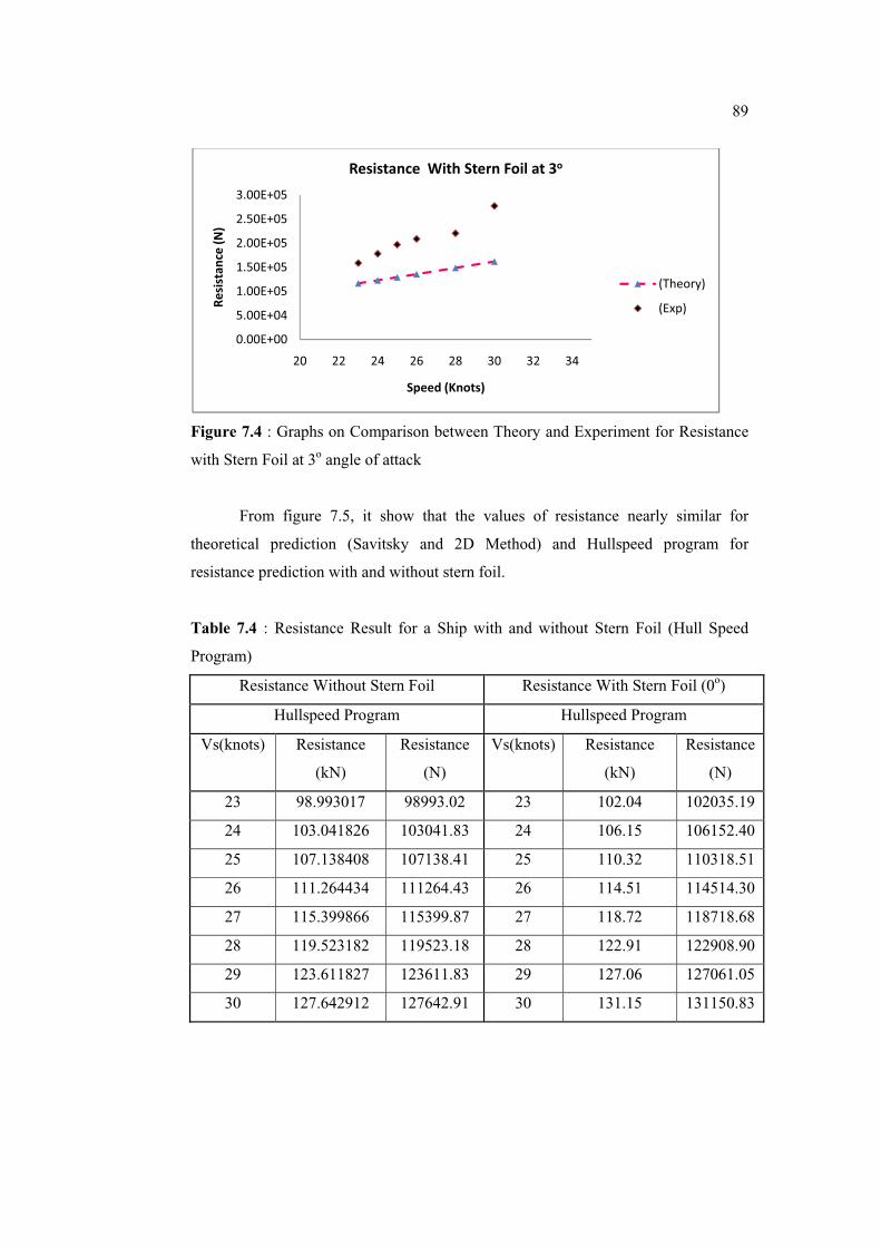
89��


with Stern Foil at 3o angle of attack

From figure 7.5, it show that the values of resistance nearly similar for

theoretical prediction (Savitsky and 2D Method) and Hullspeed program for

resistance prediction with and without stern foil.

Table 7.4 : Resistance Result for a Ship with and without Stern Foil (Hull Speed

Program)

Resistance Without Stern Foil Resistance With Stern Foil (0o)

Hullspeed Program Hullspeed Program

Vs(knots) Resistance

(kN)

Resistance

(N)

Vs(knots) Resistance

(kN)

Resistance

(N)

23 98.993017 98993.02 23 102.04 102035.19

24 103.041826 103041.83 24 106.15 106152.40

25 107.138408 107138.41 25 110.32 110318.51

26 111.264434 111264.43 26 114.51 114514.30

27 115.399866 115399.87 27 118.72 118718.68

28 119.523182 119523.18 28 122.91 122908.90

29 123.611827 123611.83 29 127.06 127061.05

30 127.642912 127642.91 30 131.15 131150.83

0.00E+00

5.00E+04

1.00E+05

1.50E+05

2.00E+05

2.50E+05

3.00E+05

20 22 24 26 28 30 32 34

Resistan

ce�(N

)

Speed�(Knots)

Resistance��With�Stern�Foil�at�3o

(Theory)

(Exp)

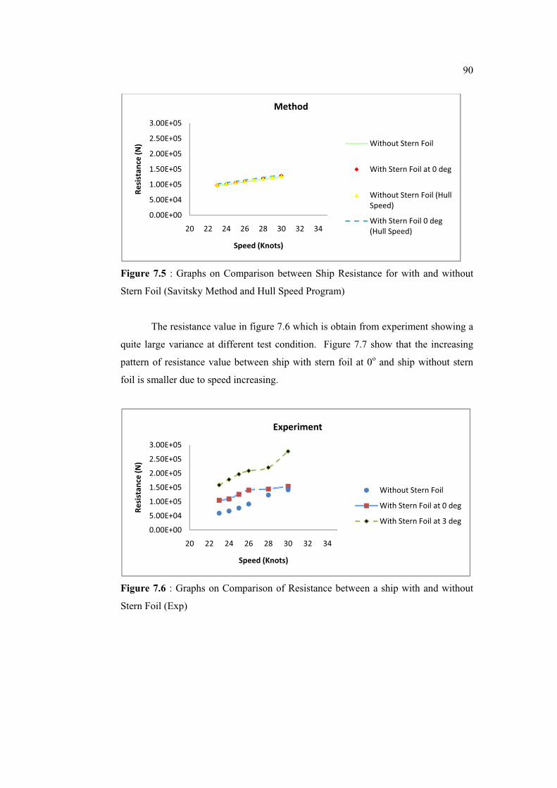
90��

Figure 7.5 : Graphs on Comparison between Ship Resistance for with and without

Stern Foil (Savitsky Method and Hull Speed Program)

The resistance value in figure 7.6 which is obtain from experiment showing a

quite large variance at different test condition. Figure 7.7 show that the increasing

pattern of resistance value between ship with stern foil at 0o and ship without stern

foil is smaller due to speed increasing.

Figure 7.6 : Graphs on Comparison of Resistance between a ship with and without

Stern Foil (Exp)

0.00E+00

5.00E+04

1.00E+05

1.50E+05

2.00E+05

2.50E+05

3.00E+05

20 22 24 26 28 30 32 34

Resistan

ce�(N

)

Speed�(Knots)

Method

Without�Stern�Foil

With�Stern�Foil�at�0�deg

Without�Stern�Foil�(Hull�Speed)

With�Stern�Foil�0�deg�(Hull�Speed)

0.00E+00

5.00E+04

1.00E+05

1.50E+05

2.00E+05

2.50E+05

3.00E+05

20 22 24 26 28 30 32 34

Resistan

ce�(N

)

Speed�(Knots)

Experiment




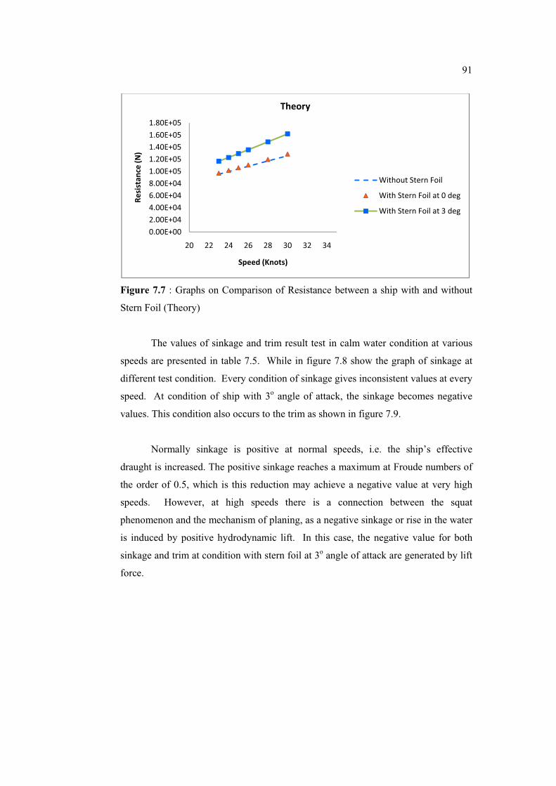
91��

Figure 7.7 : Graphs on Comparison of Resistance between a ship with and without

Stern Foil (Theory)

The values of sinkage and trim result test in calm water condition at various

speeds are presented in table 7.5. While in figure 7.8 show the graph of sinkage at

different test condition. Every condition of sinkage gives inconsistent values at every

speed. At condition of ship with 3o angle of attack, the sinkage becomes negative

values. This condition also occurs to the trim as shown in figure 7.9.

Normally sinkage is positive at normal speeds, i.e. the ship’s effective

draught is increased. The positive sinkage reaches a maximum at Froude numbers of

the order of 0.5, which is this reduction may achieve a negative value at very high

speeds. However, at high speeds there is a connection between the squat

phenomenon and the mechanism of planing, as a negative sinkage or rise in the water

is induced by positive hydrodynamic lift. In this case, the negative value for both

sinkage and trim at condition with stern foil at 3o angle of attack are generated by lift

force.

0.00E+002.00E+044.00E+046.00E+048.00E+041.00E+051.20E+051.40E+051.60E+051.80E+05

20 22 24 26 28 30 32 34

Resistan

ce�(N

)

Speed�(Knots)

Theory




92��

Table 7.5 : Sinkage and Trim Result for a Ship with and without Stern Foil

EXPERIMENT

Vs(knots)Without Stern Foil With Stern Foil 0

o With Stern Foil 3

o

Sinkage Trim Sinkage Trim Sinkage Trim

23 -0.0018 0.9975 0.0019 1.6361 -0.0009 -0.5620

24 -0.0018 0.9580 0.0024 1.4928 -0.0002 -0.6279

25 -0.0006 0.9003 0.0020 1.4572 -0.0002 -0.8416

26 -0.0004 0.9477 0.0062 1.4970 0.0001 -1.0479

28 0.0018 0.8569 0.0059 1.5462 -0.0004 -1.2637

30 0.0028 0.9352 0.0075 1.6442 0.0031 -1.6898

Figure 7.8 : Graphs on Comparison of Sinkage between a ship with and without

Stern Foil

Figure 7.9 : Graphs on Comparison of Trim between a ship with and without Stern

Foil

�0.0040

�0.0020

0.0000

0.0020

0.0040

0.0060

0.0080

20 21 22 23 24 25 26 27 28 29 30

Amplitud

e�(m

)

Ship�Speed

Sinkage


Stern�Foil�0�Deg


�2.00

�1.50

�1.00

�0.50

0.00

0.50

1.00

1.50

2.00

20 21 22 23 24 25 26 27 28 29 30

Amplitud

e�(Deg)

Ship�Speed

Trim




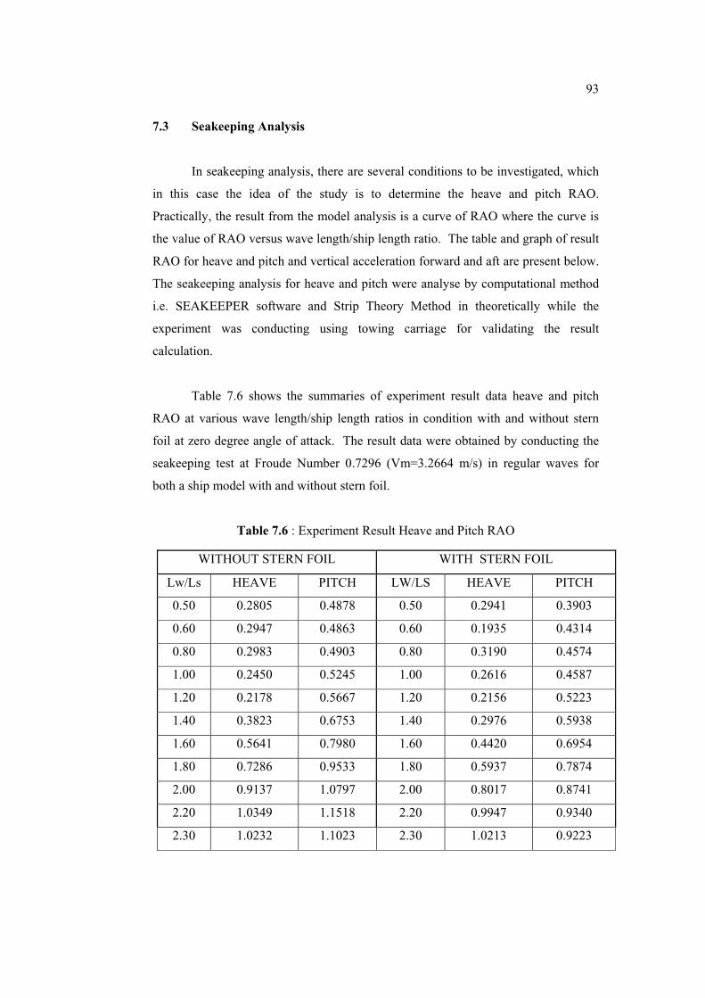
93��

7.3 Seakeeping Analysis

In seakeeping analysis, there are several conditions to be investigated, which

in this case the idea of the study is to determine the heave and pitch RAO.

Practically, the result from the model analysis is a curve of RAO where the curve is

the value of RAO versus wave length/ship length ratio. The table and graph of result

RAO for heave and pitch and vertical acceleration forward and aft are present below.

The seakeeping analysis for heave and pitch were analyse by computational method

i.e. SEAKEEPER software and Strip Theory Method in theoretically while the

experiment was conducting using towing carriage for validating the result

calculation.

Table 7.6 shows the summaries of experiment result data heave and pitch

RAO at various wave length/ship length ratios in condition with and without stern

foil at zero degree angle of attack. The result data were obtained by conducting the

seakeeping test at Froude Number 0.7296 (Vm=3.2664 m/s) in regular waves for

both a ship model with and without stern foil.

Table 7.6 : Experiment Result Heave and Pitch RAO

WITHOUT STERN FOIL WITH STERN FOIL

Lw/Ls HEAVE PITCH LW/LS HEAVE PITCH

0.50 0.2805 0.4878 0.50 0.2941 0.3903

0.60 0.2947 0.4863 0.60 0.1935 0.4314

0.80 0.2983 0.4903 0.80 0.3190 0.4574

1.00 0.2450 0.5245 1.00 0.2616 0.4587

1.20 0.2178 0.5667 1.20 0.2156 0.5223

1.40 0.3823 0.6753 1.40 0.2976 0.5938

1.60 0.5641 0.7980 1.60 0.4420 0.6954

1.80 0.7286 0.9533 1.80 0.5937 0.7874

2.00 0.9137 1.0797 2.00 0.8017 0.8741

2.20 1.0349 1.1518 2.20 0.9947 0.9340

2.30 1.0232 1.1023 2.30 1.0213 0.9223

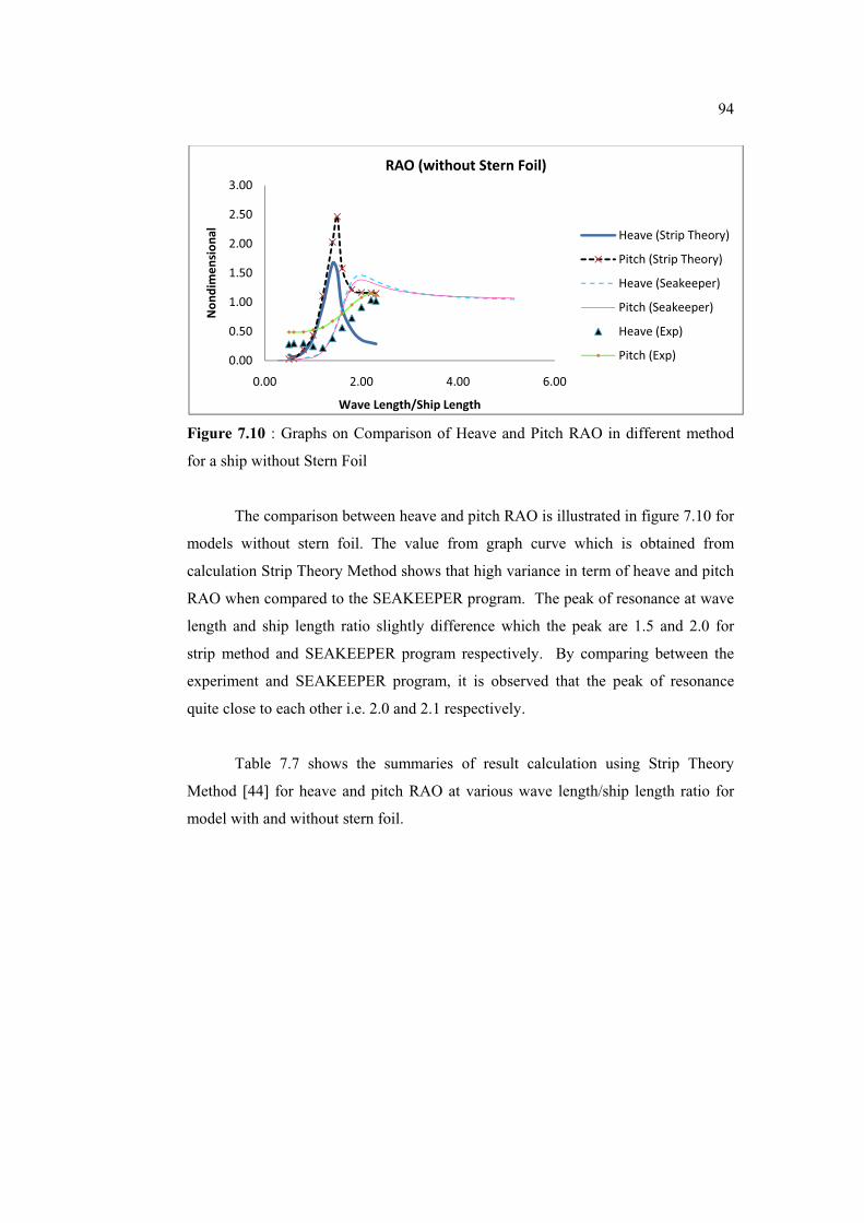
94��

Figure 7.10 : Graphs on Comparison of Heave and Pitch RAO in different method

for a ship without Stern Foil

The comparison between heave and pitch RAO is illustrated in figure 7.10 for

models without stern foil. The value from graph curve which is obtained from

calculation Strip Theory Method shows that high variance in term of heave and pitch

RAO when compared to the SEAKEEPER program. The peak of resonance at wave

length and ship length ratio slightly difference which the peak are 1.5 and 2.0 for

strip method and SEAKEEPER program respectively. By comparing between the

experiment and SEAKEEPER program, it is observed that the peak of resonance

quite close to each other i.e. 2.0 and 2.1 respectively.

Table 7.7 shows the summaries of result calculation using Strip Theory

Method [44] for heave and pitch RAO at various wave length/ship length ratio for

model with and without stern foil.

0.00

0.50

1.00

1.50

2.00

2.50

3.00

0.00 2.00 4.00 6.00

Non

dimen

sion

al

Wave�Length/Ship�Length�

RAO�(without�Stern�Foil)�

Heave�(Strip�Theory)

Pitch�(Strip�Theory)

Heave�(Seakeeper)

Pitch�(Seakeeper)

Heave�(Exp)

Pitch�(Exp)

95��

Table 7.7 : Calculation Result Heave and Pitch RAO (Strip Theory)

Lw/Lm

Strip Theory Method

Heave RAO Pitch RAO

0.50 0.0970 0.0278

0.60 0.0678 0.0333

0.80 0.1407 0.1889

1.00 0.3921 0.4361

1.20 0.9304 1.1083

1.40 1.6631 2.0278

1.50 1.5314 2.4639

1.60 0.8961 1.5776

1.80 0.5249 1.2139

2.00 0.3555 1.1639

2.20 0.3060 1.1583

2.30 0.2869 1.1500

The comparison of SEAKEEPER program and experiment for heave RAO

curves in regular waves with and without a stern foil are shown in figure 7.11 and

7.12. From experiment result, by adding a stern foil to the model causes reduction of

heave RAO at 1.6 wave length to ship length ratio which the heave RAO reduce to

3.88% compared to model without stern foil. While SEAKEPER program estimate

the reducing of heave RAO is 21.59% at 2.0 wave length to ship length ratio. This

condition occurs due to the hydrodynamic lift react to the foil as a damping in order

to reduce the vertical movement of the model.

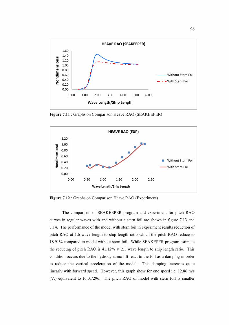
96��

Figure 7.11 : Graphs on Comparison Heave RAO (SEAKEEPER)

Figure 7.12 : Graphs on Comparison Heave RAO (Experiment)

The comparison of SEAKEEPER program and experiment for pitch RAO

curves in regular waves with and without a stern foil are shown in figure 7.13 and

7.14. The performance of the model with stern foil in experiment results reduction of

pitch RAO at 1.6 wave length to ship length ratio which the pitch RAO reduce to

18.91% compared to model without stern foil. While SEAKEPER program estimate

the reducing of pitch RAO is 41.12% at 2.1 wave length to ship length ratio. This

condition occurs due to the hydrodynamic lift react to the foil as a damping in order

to reduce the vertical acceleration of the model. This damping increases quite

linearly with forward speed. However, this graph show for one speed i.e. 12.86 m/s

(Vs) equivalent to Fn:0.7296. The pitch RAO of model with stern foil is smaller

0.000.200.400.600.801.001.201.401.60

0.00 1.00 2.00 3.00 4.00 5.00 6.00

Non

dimen

sion

al

Wave�Length/Ship�Length

HEAVE�RAO�(SEAKEEPER)


With�Stern�Foil

0.00

0.20

0.40

0.60

0.80

1.00

1.20

0.00 0.50 1.00 1.50 2.00 2.50

Non

dimen

sion

al


HEAVE�RAO�(EXP)


With�Stern�Foil

97��

compared to the model without stern foil, meaning that the pitch RAO of model

incorporating with stern foil is able to reduce the motion.

Figure 7.13 : Graphs on Comparison Pitch RAO (SEAKEEPER)

Figure 7.14 : Graphs on Comparison Pitch RAO (Experiment)

0.000.200.400.600.801.001.201.401.60

0.00 1.00 2.00 3.00 4.00 5.00 6.00

Non

dimen

sion

al


PITCH�RAO�(SEAKEEPER)


With�Stern�Foil

0.00

0.20

0.40

0.60

0.80

1.00

1.20

1.40

0.00 0.50 1.00 1.50 2.00 2.50

Non

dimen

sion

al

Wave�Length/Ship�Length�

PITCH�RAO�(EXP)


With�Stern�Foil

98��

Figure 7.15 : Graphs on Comparison Pitch RAO between Experiment, Strip Theory

and SEAKEEPER Program

Figure 7.15 and 7.16 show the heave and pitch RAO in term of comparison of

method determination for the model without stern foil. Each graph curves had their

own self characteristic where different methods are used to predict or calculates the

response frequency of waves. From this graph curves, the result of Strip Theory

show high different compared to the experiment and SEAKEEPER program. The

peak resonance in every method is contradictory especially using Strip Theory.

However, each heave and pitch RAO in experiment is lower compared to

SEAKEEPER program and Strip Theory Method.

The result from Strip Theory become greater compare to other method due to

transom and viscous effect that not taken into account in this calculation.

Theoretically, the waves flow around a ship which the waves produce incident

exciting forces, diffract when they reach the ship hull, which also produces forces on

it, and the waves produce ship motion. These motions also produce radiated waves,

which again produce forces.

0.00

0.50

1.00

1.50

2.00

2.50

3.00

0.00 1.00 2.00 3.00 4.00

Non

dimen

sion

al


PITCH�RAO�(without�Stern�Foil)��

Exp

Strip�Theory

Seakeeper�Program

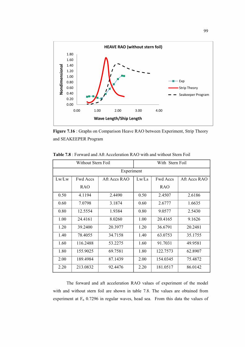
99��

Figure 7.16 : Graphs on Comparison Heave RAO between Experiment, Strip Theory

and SEAKEEPER Program

Table 7.8 : Forward and Aft Acceleration RAO with and without Stern Foil

Without Stern Foil With Stern Foil

Experiment

Lw/Lw Fwd Accs

RAO

Aft Accs RAO Lw/Ls Fwd Accs

RAO

Aft Accs RAO

0.50 4.1194 2.4490 0.50 2.4507 2.6186

0.60 7.0798 3.1874 0.60 2.6777 1.6635

0.80 12.5554 1.9384 0.80 9.0577 2.5430

1.00 24.4161 8.0260 1.00 20.4165 9.1626

1.20 39.2400 20.3977 1.20 36.6791 20.2481

1.40 78.4055 34.7158 1.40 63.0753 35.1755

1.60 116.2488 53.2275 1.60 91.7031 49.9581

1.80 155.9025 69.7581 1.80 122.7573 62.8907

2.00 189.4984 87.1439 2.00 154.0345 75.4872

2.20 213.0832 92.4476 2.20 181.0517 86.0142

The forward and aft acceleration RAO values of experiment of the model

with and without stern foil are shown in table 7.8. The values are obtained from

experiment at Fn 0.7296 in regular waves, head sea. From this data the values of

0.00

0.20

0.40

0.60

0.80

1.00

1.20

1.40

1.60

1.80

0.00 1.00 2.00 3.00 4.00

Non

dimen

sion

al


HEAVE�RAO�(without�stern�foil)

Exp

Strip�Theory

Seakeeper�Program

100��

RAO either forward or aft acceleration are increased due to wave length. Both graph

curves in figure 7.17 and 7.18 shows decreasing of forward and aft acceleration RAO

by increasing the wave length when the model with stern foil. By adapting the stern

foil at the model, the forward and aft RAO reduces to 21.1% and 6.14% respectively.

The situation occurs due to reducing of trim angle where lift force exerted to the

model by lifting effect .Hence a small reduction in trim angle may reduce the impact

acceleration significantly. By inserting the stern foil can therefore be very effective in

reducing the trim angle, thereby decreasing the impact forces.

Figure 7.17 : Graphs on Comparison Forward Acceleration RAO

Figure 7.18 : Graphs on Comparison Aft Acceleration RAO

0

50

100

150

200

250

0.00 0.50 1.00 1.50 2.00 2.50

RAO

Forward�Acceleration��


With�Stern�Foil

0

20

40

60

80

100

0.00 0.50 1.00 1.50 2.00 2.50

RAO

Wave�Length/�Ship�Length

Aft��Acceleration��


With�Stern�Foil

101��

The stern foil is most efficient in damping vertical motion where it is proven

in motion reduction technique. In this case, the stern foil is able to reduce the

amplitude of heave, pitch, forward and aft acceleration. The experimental result

show that at wave length 3.689 m, height waves 0.0654 m and wave period 1.45 s,

the motion of the vessel automatically trim down. This condition resulting good

indication that stern foil will reduced the motion in term of heave, pitch, forward and

aft acceleration. Figure 7.19, 7.20, 7.21 and 7.22 show that the variance of amplitude

in every RAO for model with and without stern foil.

Figure 7.19 : Record Curves of Heave Amplitude

�1.50E�02

�1.00E�02

�5.00E�03

0.00E+00

5.00E�03

1.00E�02

1.50E�02

2.00E�02

0 20 40 60 80 100Heave�(m

)

Running�No

Lw=3.689,Hw=0.0654,Tw=1.45s

With�Stern�Foil


102��

Figure 7.20 : Record Curves of Pitch Amplitude

Figure 7.21 : Record Curves of Forward Acceleration Amplitude

0.00E+00

5.00E�01

1.00E+00

1.50E+00

2.00E+00

2.50E+00

3.00E+00

3.50E+00

0 20 40 60 80 100

Pitch�(0

o )

Running�No

Lw=3.689,Hw=0.0654,Tw=1.45s

With�Stern�Foil


�0.5

�0.4

�0.3

�0.2

�0.1

0

0.1

0.2

0.3

0.4

0 20 40 60 80 100

Forw

ard�Acc��(ms�2 )

Running�No

Lw=3.689,Hw=0.0654,Tw=1.45s

With�Stern�Foil


103��

Figure 7.22 :Record Curves of Aft Acceleration Amplitude


From the tables and graphs above, the performance prediction of high speed

craft can be materialized. The performance prediction of high speed craft in term of

resistance and seakeeping are a challenging work where many aspects or parameters

should to be taken into account on calculation especially the ones which are involve

in modification work. Even though Strip Theory and motion prediction software can

be used to optimise hullforms for resistance and seakeeping performance but it is

being simplified due to linearization of formulation. However, in this case, the

SEAKEEPER program is quite precise in predicting the ship motion. By

incorporating the stern foil it can have significantly better performance even though

it will affect the resistance performance at slow speed but resulting good

performance in seakeeping quality at high speed.

�3.00E�01

�2.00E�01

�1.00E�01

0.00E+00

1.00E�01

2.00E�01

3.00E�01

0 20 40 60 80 100

Aft��A

cc��(ms�2 )

Running�No

Lw=3.689,Hw=0.0654,Tw=1.45s

With�Stern�Foil


CHAPTER 8

CONCLUSION

8.1 Conclusion

Performance prediction on high speed craft especially in planing craft is

difficult to achieve for both resistance and seakeeping. The performance becomes a

challenging work if the craft has special or unique hull form. The study on planing

craft was conducted on exclusive hullform which is called M Hull. The objective of

this research is to predict the performance of the planing craft M Hull in term of

resistance and seakeeping for different test condition (with and without stern foil).

Generally, many of the hypothesis and linearization that can be made for

conventional craft are not applicable especially for vessel that has modification on it

hullform, and great care has to be taken to ensure that the predictions are reliable and

the way in which the experiment was conducted. In order to carry out the

performance prediction for certain vessel, special techniques have to be developed

for the experiments associated with the prediction of the performance of high speed

craft.

By incorporating the stern foil (0o angle of attack) on the model, the

resistance is slightly higher compared to the model without stern foil. However, the

increasing patterns of resistance becoming less at high speed, which is at speed 30

105

��

knots, the resistance percentage is increased only at 8% (refer table 7.1 and 7.2). The

resistance predictions using theoretical formulation (Savitsky and two dimensional

Method) give nearly precise value to the experimental result for both models. The

Hull Speed program and theory also resulting quite similar resistance value (see table

7.4 and figure 7.5).

Experiment and software program (SEAKEEPER) results show that the

contributions of stern foil reduce the heave, pitch, forward and aft acceleration of the

M-Hull planing craft in waves is important. In this study, the model speed at 3.2664

m/s (Fn=0.7296), SEAKEEPER result show heave and pitch RAO reducing 21.59%

and 41.12% respectively. While the reducing of heave and pitch RAO in experiment

are 3.8% and 18.91% respectively (see figure 7.12 and 7.14). Even though the

percentage between SEAKEEPER is quite large but both method show the reducing

pattern on heave and pitch RAO. The forward and aft acceleration also reduce when

the model incorporate with stern foil (see figure 7.17 and 7.18).

8.2 Future Work

Based on analysis, the performance prediction especially on resistance can be

improved for further development. These are some recommendations for further

research of M-Hull planing craft with stern foil:

1. The stern foil replaced by controllable stern foil with Proportional Integration

Derivatives (PID) control system.

2. Conduct the model test beyond Fn>1.0.

3. Carry out advance research on dynamic instability, propulsion and

manoeuvring performance for the model with Stern Foil.

REFERENCES

[1] B.R Clayton and RED Bishop “Mechanics of Marine Vehicle” University

College London, May 1981.

[2] Newton R.N “The combination of Sail with an alternative source of power”

by K.C Barnaby, Trans. Royal Institution Naval Architecture, 104, 90-2, 1962.

[3] Mandel, P. “Water, air and Interface Vehicle” MIT Press, Boston 1962.

[4] Clement, E.P and Pope, J.D “Stepless and stepped Planing Hulls-Graphs for

Performances Prediction and Design” David Taylor Model Basin- Rep-1490 –1961.

[5] Savitsky D, and Brown, P.W “Procedure of Hydrodynamic Evaluation of

Planning Hull in smooth and rough water” Marine Technology, 13(4), 381-400 Oct

1976.

[6] International Maritime Organisation “Safety Measures of High Speed Craft

2000 ” SOLAS Chapter X-429-431, Jul 2004.

[7] Koelbel, J.G. [1971], “Seakeeping Considerations in Design and Operation of

Hard Chine Planing Hulls”, Small Craft Engineering Report (120) ‘Performance

Prediction’,University of Michigan, Michigan, 1971

[8] Thomas, C.G. and Bruce, J. [1982], “Introduction to Naval Architecture”, E.

& F.N. Spon Ltd, London, 1982

[9] Valdenazzi, F., et al [2001], “Seakeeping Optimisation of Fast Vessels by

Means of Parametric Modeling”, PRADS 2001, Shanghai, September 2001

[10] Savitsky, D “Hydrodynamic Design of Planning Hull.” Marine Technology

Vol. 8, No.4 Oct 1964.

107

[11] A.R.J M Llyord “Seakeeping Ship Behaviour in Rough Weather”. Revised

Edition Ellis Horwood Limited page 359-368, 1998.

[12] J.A. Keuning and J. Gerritsma “Resistance tests of a Series of Planing Hull

Forms with 25 degrees Deadrise Angle” International Shipbuilding Progress 29 (1982), 337.

[13] J.A. Keuning, J. Gerritsma and P.F. van Terwisga “Resistance Tests of a

Series of Planing Hull Forms with 30 degrees Deadrise Angle and a Calculation

Method Based on this and Similar Series” International Shipbuilding Progress 40 (1993), 333–385.

[14] E.P. Clement and D.L. Blount, “Resistance Tests of a Series of Planing Hull Forms” Transactions SNAME, 1953.

[15] J.A Keuning “Grinding the Bow or How to improve the Operability of fast

Monohull” International Shipbuilding Progress 53 (2006), 281-310.

[16] E.E. Zarnick “A Non Linear Mathematical Model of Planing Boats in Regular

Head Waves” David Taylor Naval Ship Research and Development Center Report

78-032, March 1982.

[17] J.A. Keuning “Nonlinear Heave and Pitch Motions of Fast Ships in Irregular

Head Waves” ASNE High Speed Marine Vehicles Conference, Washington, June

1992.

[17][18] J.A. Keuning “The Non Linear Behavior of Fast Monohulls in Head

Waves” PhD Thesis, Delft University of Technology, September 1994.

[19] Karafiath, G., D. S. Cusanelli, and C. W. Lin. 1999. “Stern Wedges and Stern

Flaps for Improved Powering – U.S. Navy Experience” SNAME Annual Meeting.

Baltimore.

[20] Cave, W. L., and D. S. Cusanelli. 1993. “Effect of Stern Flaps on Powering

Performance of the FFG-7 Class” Marine Technology. 30(1): 39-50.

[21] Cusanelli, D. S., S. D. Jessup, and S. Gowing. 1999 “Exploring

Hydrodynamic Enhancements to the USS ARLEIGH BURKE (DDG 51)” FAST’99, Fifth International Conference on Fast Sea Transportation, Seattle.

[22] Omar Yaakob, Suhaili Shamsuddin & Koh Kho King “Stern Flap for

Resistance Reduction of Planing Hull Craft: A Case Study With A Fast Crew Boat

Model” Jurnal Teknologi, 41(A) Dis. 2004: 43–52 © Universiti Teknologi Malaysia.

[23] Wang Long-Wen, “A Study on Motion of High Speed Planing Boats with

Controllable Flaps in Regular Waves” ISP. 1985 Vol. 32-365-6.

108

[24] Odd M. Faltinsen “Hydrodynamics of High Speed Marine Vehicles”

NorweigenUniversity of Sciene and Technology, Cambridge University Press 2005,

pp 171-166.

[25] David Vacanti “Foil Design Parameters and Performance” Sail Magazine

August 1985

[26] “Seakeeper User Manual” Formation Design System Maxsurf, 2006.

[27] Predrag Bojovic and Prasanta K. Saho “Regression Analysis of Systematic

Series Calm Water Performance” Third International Symposium on Performance

enhancement for Marine application May, 1997.

[28] P. Van Oossanen “Resistance Prediction of Small High speed Displacement

Vessel, State of Art” The Symposium on the impact of 200 miles economic zone,

RINA (Australian branch) and Institute of Marine Engineers, July 1979.

[29] Korvin, Kroukovsky, B.V, Savitsky,D. and Lehman, W.F. “Wetted area and

Center of Pressure of Planing Surface” Steven Institute Of Technology Davidson

Laboratory report No 360, Aug 1949.

[30] Murray, A.B. “The Hydrodynamic of Planing Hull” SNAME trans. Vol. 58,

1950.

[31] Savitsky, D and Neidinger, J.W “Wetted area center of pressure of planning

at very slow speed coefficient,” Steven institute of technology, Davidson Laboratory

report No 493, Jul 1954.

[32] Hadler, J.B “The Prediction of Power Performance of Planing Craft” SNAME

Trans. Vol. 74, 1966.

[33] Savitsky D and Brown PW “Procedures of Hydrodynamic Evaluation of

Planing Hull in Smooth and Rough Water” Marine Technology, Vol 23, No 4, Oct

1976.

109

[34] Ood M. Faltinsen “Hydrodynamic of High Speed Marine Vehicles”

Cambridge published 2005 pp 176-200.

[35] Tuck E.O “A Strip Theory for Wave Resistance” in Procedure 3rd

International Workshop on Water waves and Floating body, pp169-74, MIT, 1988.

[36] Newman JN “Marine Hydrodynamic” Cambridge The MIT Press, 1977.

[37] Michell JM “The Waves Resistance of a Ship” Phil Magazine, London, Series

5,45, pp 106-23 (1898).

[38] Weissinger, J., “The Lift Distribution of Swept-back Wings” NACA TM-

1120, 1947.

[39] Hoerner “Fluid Dynamic Drag” Published by the author, 1965.

[40] Rawson K.J and Tupper E.C “Basic ship theory” Fifty Edition Heineman,

2001.

[41] A.R.J M Llyord “Seakeeping Ship Behaviour in Rough Weather”. Revised

Edition Ellis Horwood Limited,1998.

[42] Adi Maimun “Stability of fishing Vessel in a Astern Sea shallow water

Environment“ University of Strathyclyd Glasglow ,phd Thesis,1993.

[43] Adi Maimun “Lecture note: Dynamics of Marine Vehicles” University

Teknologi Malaysia Skudai 2008

[44] Bhattacharyya R. “Dynamics of Marine Vehicle” A Wiley Intersciene

Publication, Nov 1972.

��

APPENDIX A

Details Planning for Project I and II

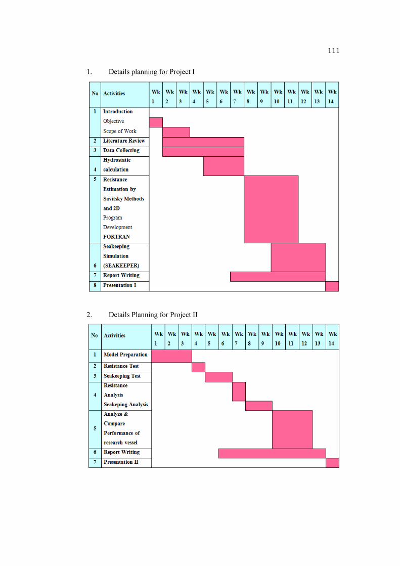
FFF��1. Details planning for Project I

2. Details Planning for Project II

APPENDIX B

Resistance and Seakeeping Test

113�

1.0 Designation

Model Test of a Planing Craft (M Hull), Model MTL- 046 (Resistance and

Seakeeping Test)

2.0 Objectives

The resistance test of a planing craft model is carried out to determine:

a. The required total resistance a full scale of bare hull of planing craft (M Hull)

at corresponding speeds in calm water.

b. The required total resistance of a full scale of planing craft of full scale of

planing craft with and without stern foil at 25 knots in regular waves.

The seakeeping test for model is carried out to determine:

a. The significant effect of motions (heave,pitch RAO) in regular waves (head

seas) at various wavelength at design speed 25 knots with and without stern foil.

b. Forward and aft acceleration in regular waves at design speed 25 knots with

and without stern foil.

c. To present the result of the Response Amplitude Operators for the both model

according to a and b.

3.0 Introduction

Model testing in towing tank is one of the essential parts in ship design

process and resistance test is needed in determining the resistance and power

effective of the ship. To confirm design predictions of powering requirement, scaled

model resistance test are carried out. Measurement of resistance of planing craft,

model MTL- 046 is undertaken and the data/results are analyzed accordingly to

obtain full-scaled resistance. Analysis is to be carried out using ITTC 1957 method.

114�

Another model test that can be carryout is seakeeping test. Actually this test

is to measure the behavior of the vessel at seas. Model testing provides an attractive

alternative. The seakeeping test can predict the characteristics of the vessel in term

of motion which is it gives significant effect of motion. The success of a ship design

depends ultimately on its performance in a seaway. However, the in a realistic

seaway is such a complex problem that ship designers are generally forced to select

their hull forms and ship dimensions on the basis of calm water performance without

much consideration of the sea and the weather conditions. Only very recently

sophisticated experimental techniques such as seakeeping test and computer

applications in ship motion theories have made it possible for the designer to

consider the seakeeping qualities of his ship at an early stage.

In this model testing, the resistance test will be conducted at bare hull with

and without stern foils in various speed at calm water, while seakeeping test will be

carryout in three conditions at cruising speed (25 knots) in regular waves. The model

test will be conducted in order to optimize the performance at high speed condition.

3.1. Resistance

The resistance of a ship at a given speed can be defined as a force required to

tow the ship at that speed in smooth water, assuming no interference from the towing

ship. The power necessary to overcome this resistance is called the tow rope or

effective power. This total resistance is consists of a number of different components,

which is caused by a variety of factors and which interact one with other in a

complicated way. In simplified manner, it is usual to consider the total calm water

resistance inclusive four main components;

a. The frictional resistance, due to the motion of the hull through a viscous

fluid.

b. The wave making resistance, due to the energy created continuously on the

surface of water by the ship to the wave system.

c. Eddy resistance, due to the energy carried away by eddies shed from the

hull or appendages. Local eddying will occur behind appendages such as bossing,

115�

shaft struts, and fro stern frames and rudders if these items are not properly

streamlined and aligned with the flow.

d. Air resistance experienced by the above water line of the main hull and

superstructures due to the motion of the ship through air.

The resistance from ii), iii) and iv) commonly can be taken together under the

term known as residuary resistance. Figure 1 can be referred to give us clearer picture

about the total resistance of the ship and its components related.

The given summary of the total resistance is convenient but not scientifically

correct since the first three types all react one with the other. It can be seen where the

skin drag gives rise to a boundary layer which virtually alters the shape of the hull and

hence the pressure distribution and the resulting wave making resistance. Also the

wave system alters the wetted surface area and so the skin friction of the ship

resistance. Nevertheless, it is convenient to make such division for practical use, but

the presence and interaction of all these factors well illustrated the complexity of the

ship resistance problem.

Figure 1 Basic component of Resistance

The practical methods whereby model tests are carried out at full scale

Froude number and corrections made for the differences in Reynold’s number are

given. The method originally used by William Froude is applied, and then its modern

derivative and finally that by Hughes is extended. The basic and early approach,

Total Resistance

Frictional Resitance Residuary Resistance

Eddy RessitanceWave- making Resistance

Air Resistance

116�

suggested by Froude which breakdown of resistance into several components,

assuming:

Total Resistance = Skin Friction + “The Rest”, which he termed Residuary

i.e.

CT = *CF + CR*

The skin friction coefficient (CF) is estimated from data for a flat plate of

same length, wetted surface area and velocity of model or ship. The difference

between total resistance and skin friction gives the residual resistance. Hence the part

dependent on Reynold’s number is separately determined and the model test is

carried out at the corresponding velocity which gives equality of Fn for ship and

model. Hence dynamic similarities for wave-making (or residuary resistance) is

obtained.

Hence if residuary resistance is considered,

Model:

Ship:

is constant, g is constant, f2 same for ship and model (i.e. same Fn) and it follows

that:

or

Then,

117�

Froude’s law; when speeds of ship and model are in ratio of square root of

their lengths, then resistance due to wave-making varies as their displacements.

(Speeds in ratio of square root of lengths called “corresponding speeds”). In

coefficient form:

LVLS �� 22 , (due to same Fn), hence �� 32

21

LSV ��

Thus,

for constant L

V

L

V ,2

i.e. CRM = CRS same for model and ship at constant L

V

Now, CTM = (1+k)CFM + CRM

And CTS = (1+k)CFS + CRS

but, *CRM = CRS*

Hence, total ship resistance can be determined by following equation:

Rts = Cts*0.5*�*S*V2

3.2. Seakeeping

Seakeeping is the dynamic response of the ship affected by

environmental forces, primarily wind and waves. It is often a limiting factor in

operability, specifically speed loss. By incorporating seakeeping into the initial ship

design, the ship’s performance and efficiency can improve. The primary parameters

that affect seakeeping are the ship proportions, including waterplane geometry and

weight distribution. Secondarily, unique hull characteristics such as transom sterns,

bulbous bows or motion damping devices also affect the ship’s seakeeping abilities.

There are some general seakeeping design guidelines that should be always kept in

mind during the design process.

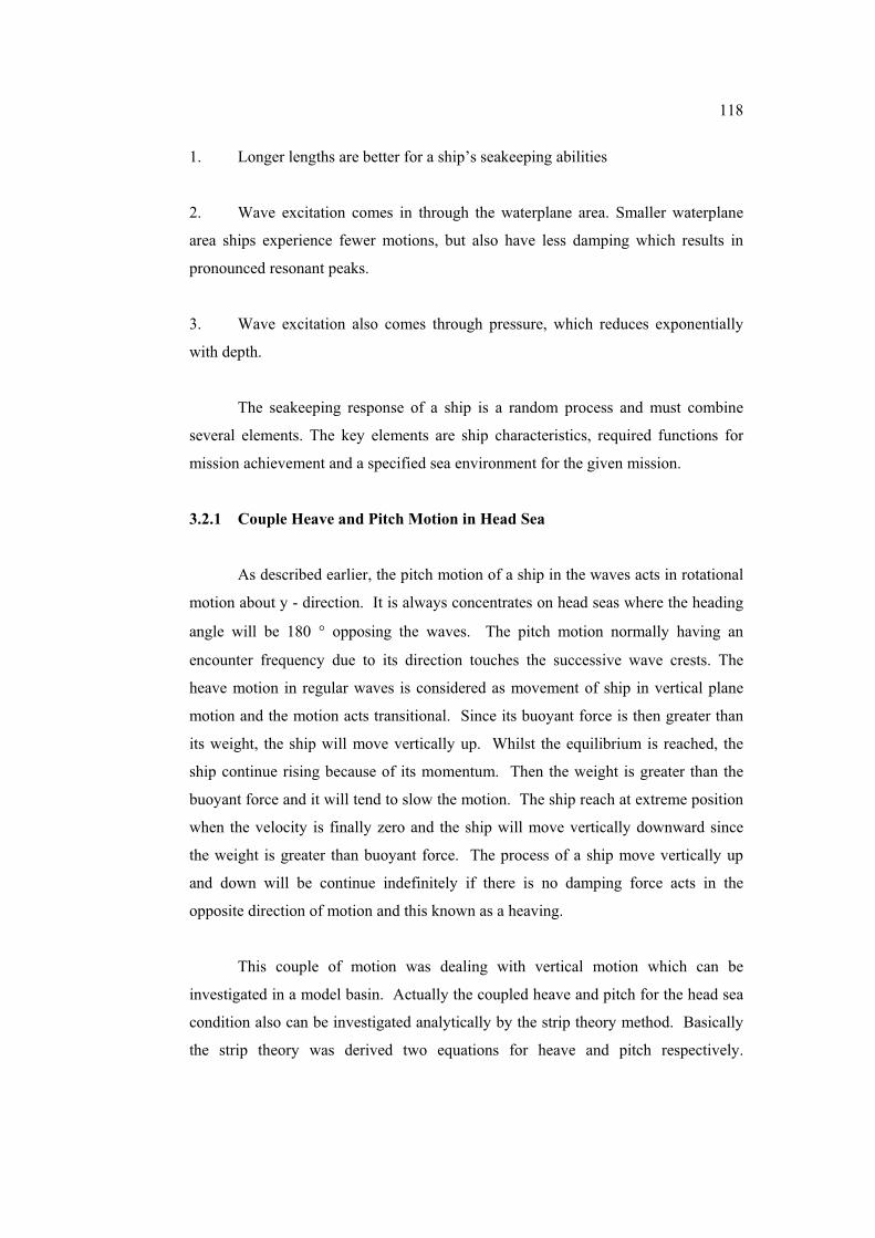
118�

1. Longer lengths are better for a ship’s seakeeping abilities

2. Wave excitation comes in through the waterplane area. Smaller waterplane

area ships experience fewer motions, but also have less damping which results in

pronounced resonant peaks.

3. Wave excitation also comes through pressure, which reduces exponentially

with depth.

The seakeeping response of a ship is a random process and must combine

several elements. The key elements are ship characteristics, required functions for

mission achievement and a specified sea environment for the given mission.

3.2.1 Couple Heave and Pitch Motion in Head Sea

As described earlier, the pitch motion of a ship in the waves acts in rotational

motion about y - direction. It is always concentrates on head seas where the heading

angle will be 180 � opposing the waves. The pitch motion normally having an

encounter frequency due to its direction touches the successive wave crests. The

heave motion in regular waves is considered as movement of ship in vertical plane

motion and the motion acts transitional. Since its buoyant force is then greater than

its weight, the ship will move vertically up. Whilst the equilibrium is reached, the

ship continue rising because of its momentum. Then the weight is greater than the

buoyant force and it will tend to slow the motion. The ship reach at extreme position

when the velocity is finally zero and the ship will move vertically downward since

the weight is greater than buoyant force. The process of a ship move vertically up

and down will be continue indefinitely if there is no damping force acts in the

opposite direction of motion and this known as a heaving.

This couple of motion was dealing with vertical motion which can be

investigated in a model basin. Actually the coupled heave and pitch for the head sea

condition also can be investigated analytically by the strip theory method. Basically

the strip theory was derived two equations for heave and pitch respectively.

119�

According to Newton’s second law, at any instant all vertical forces on the ship are in

dynamic equilibrium. Thus, the heaving and pitching equation can express as:

j01 -.�

�*1 A -/

Where

-. = The sum of various fluid forces (vertical hydrodynamic forces as well as the

wave excitation force)

-/ = The sum of corresponding moments acting on the vessel because of relative

motion of vessel and wave.

In order to simplified this complex motion problem several assumptions and

limitations have been made as follows:

1. The ship must be heading into the waves in a direction transverse to their

crest line.

2. The seaway is considered to consist of regular harmonic waves.

3. The ship motions of surge, sway, yaw and roll are neglected.

The general equation coupled of heaving and pitching can be expressed as:

É�n I 566Ê 01 I 76603 I 8660 I 569*1 I 769*3 I 869* A .)]+ )�99 I 599+*1 I 799*3 I 899* I 59601 I 79603 I 8960 A /)]+

For determining the effect of stern foil, calculating the coupling movement of

heave and pitch in regular waves, the effect of foil on the vessel is considered as a

small perturbation, and the motion of planing hull vessel with stern foil in waves may

be described by the following equation:

120�

É�n I 566Ê 01 I 76603 I 8660 I 569*1 I 769*3 I 869* A .)]+ I �.

)�99 I 599+*1 I 799*3 I 899* I 59601 I 79603 I 8960 A /)]+ I �/

Where, 012 032 0 = heave acceleration, velocity and displacement, respectively. *1 2 *3 2 * = pitch angular acceleration, velocity and displacement respectively.

�/g = mass of vessel. �44 = pitch inertia moment of vessel. 5662 7662 8662 5692 7692 8692 5992 7992 8992 5962 7962 896= stability derivatives �.= flap excited force �/=flap excited moment

Basically the RAO are derived from the amplitudes by dividing the motion

response by the wave input parameter:

arameterwaveinputp

onsemotionrespRAO �

The RAO for pitching, heaving and rolling are defined as below:

Pitching RAO = Pitch Amplitude / Wave Slope

a

a

k��

�

Heave RAO = Heave Amplitude / Wave Amplitude

a

az

��

4.0 Experiment Apparatus, Equipment and Facility

4.1 Towing Tank

Main dimensions of 120 m length, 4 m width and, 2.5 m depth. Detail particulars of

towing tank are shown in figure 2 and 3.

121�

Figure 2 Side view of towing tank

Figure 3 Plan view of towing tank

4.2 Towing carriage

The maximum speed of Towing Carriage is 5 m/s. At maximum acceleration,

1 m/sec2, the carriage can achieve a minimum measuring time of 10 seconds at the

maximum speed.

4.3 Data acquisition system (refer Figure 4 for the DAAS block diagram)

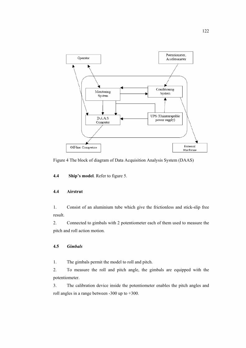
122�

Figure 4 The block of diagram of Data Acquisition Analysis System (DAAS)

4.4 Ship’s model. Refer to figure 5.

4.4 Airstrut

1. Consist of an aluminium tube which give the frictionless and stick-slip free

result.

2. Connected to gimbals with 2 potentiometer each of them used to measure the

pitch and roll action motion.

4.5 Gimbals

1. The gimbals permit the model to roll and pitch.

2. To measure the roll and pitch angle, the gimbals are equipped with the

potentiometer.

3. The calibration device inside the potentiometer enables the pitch angles and

roll angles in a range between -300 up to +300.

123�

4.6 Towing Guide

1. Towing guide is attached to the model at the center of gravity of the model.

2. The towing guide enables the model to move freely in vertical and

longitudinal direction but it keeps the model transversely in position.

3. The towing guide is fully balanced, so no force is acting on the model when

there is no movement.

4.7 Wave generator

For Seakeeping model testing, the waves are generated by a wave flap at the

end of the Towing Tank in UTM with are to generating a long crested regular and

random waves, parallel to the wave flap. The user needs to calculate the desired

waves for model test by wave calculation software before generate the waves through

wave generator. The wave calculation software can be operated from the terminals

and transform into desire waves and wave spectrum through the flap actuators. The

capabilities of wave generators to generate regular waves are at period range 0.5 sec

to 2.5 sec with a wave height corresponding to a maximum steepness of 1/10 in a

period range of 0.5 to 1.7sec. The created wave is absorbed by a wave absorber at the

other end of the tank.

The maximum wave height that can be achieved is 0.44m for wave period of

1.7sec. The wave generator of the basin is capable in generating regular and irregular

waves over period range of 0.5sec to 2.5sec. The irregular waves; characterized by a

Jonswap or a Pierson-Moskowitz spectrum can be generated up to a significant wave

height of 0.25m. Basically it consists of a hinged dry back type flap, hydraulically

driven and computer controlled.

Basically the wave generator consists of a hinged dry back type flap,

hydraulically driven and computer controlled. The wave generator of the basin is

capable of generating regular and irregular waves over a wave period range of 0.5sec

to 2.5sec.

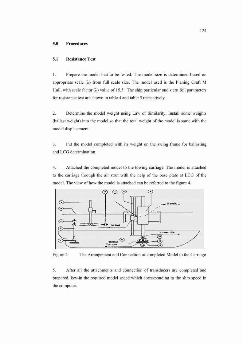
124�

5.0 Procedures

5.1 Resistance Test

1. Prepare the model that to be tested. The model size is determined based on

appropriate scale (�) from full scale size. The model used is the Planing Craft M

Hull, with scale factor (�) value of 15.5. The ship particular and stern foil parameters

for resistance test are shown in table 4 and table 5 respectively.

2. Determine the model weight using Law of Similarity. Install some weights

(ballast weight) into the model so that the total weight of the model is same with the

model displacement.

3. Put the model completed with its weight on the swing frame for ballasting

and LCG determination.

4. Attached the completed model to the towing carriage. The model is attached

to the carriage through the air strut with the help of the base plate at LCG of the

model. The view of how the model is attached can be referred to the figure 4.

Figure 4 The Arrangement and Connection of completed Model to the Carriage

5. After all the attachments and connection of transducers are completed and

prepared, key-in the required model speed which corresponding to the ship speed in

the computer.

125�

6. The model test will be carried out for 6 corresponding speeds without and

with stern foil as shown in table 1, 2 and 3:

Table 1 Summaries of Resistance Test for without Stern foil

Table 2 Resistance Test Summary for with Stern foil at angle of attack (�) 0o

Table 3 Resistance Test Summary for with Stern foil at angle of attack (�) 3o

Ship Speed,

Vs (knot)

Froude Number

(Fn)

Ship Speed, Vs

(ms¯¹)

Model Speed, Vm

(ms¯¹)

23 0.6713 11.8312 3.0051

24 0.7004 12.3456 3.1358

25 0.7296 12.8600 3.2664

26 0.7588 13.3744 3.3971

28 0.8172 14.4032 3.6584

30 0.8756 15.4320 3.9197

Ship Speed,

Vs (knot)

Froude Number

(Fn)

Ship Speed, Vs

(ms¯¹)

Model Speed , Vm

(ms¯¹)

�

23 0.6713 11.8312 3.0051 0o

24 0.7004 12.3456 3.1358 0o

25 0.7296 12.8600 3.2664 0o

26 0.7588 13.3744 3.3971 0o

28 0.8172 14.4032 3.6584 0o

30 0.8756 15.4320 3.9197 0o

Ship Speed,

Vs (knot)

Froude Number

(Fn)

Ship Speed, Vs

(ms¯¹)

Model Speed , Vm

(ms¯¹)

�

23 0.6713 11.8312 3.0051 3o

24 0.7004 12.3456 3.1358 3o

25 0.7296 12.8600 3.2664 3o

26 0.7588 13.3744 3.3971 3o

28 0.8172 14.4032 3.6584 3o

30 0.8756 15.4320 3.9197 3o

126�

7. Run the towing carriage at corresponding speed. Start the running with

model speed, Vm at 3.0051ms-1.

8. When the towing carriage speed becomes constant, approximately 10

seconds, click the “continue” button to measure and log the data into the computer.

9. After around 10 to 15 seconds running at the constant speed, click “stop” to

stop logging the data and after that slow down the towing carriage and then stop.

10. Repeat the Step 7 until 9 for difference model speed.

11. Note down all results into a table.

12. Repeat the same procedures for model with stern foil with angle of attack( )

0o and 3o.

13. From the result of the test, graph RS vs VS were plotted.

Table 4 The Main Parameters of Resistance Test

Table 5 Stern Foil Parameters

Description Ship Model

Scale ratio, � 1 15.5

Length Waterline LWL (m) 31.667 2.0430

Breadth Waterline (m) 7.4168 0.4785

Depth , D (m) 3.300 0.2129

Draught, T (m) 1.365 0.0881

Displacement (Tonne) 130.275 0.0341

Wetted surface area, S (m2) 220.000 0.9157

Longitudinal center of gravity abaft !, LCG (m) 2.258 0.1457

Vertical center of gravity (from keel) (m) 2.124 0.1370

Deadrise angle, � (deg) 14 14

Block coefficient, Cb 0.4 0.4

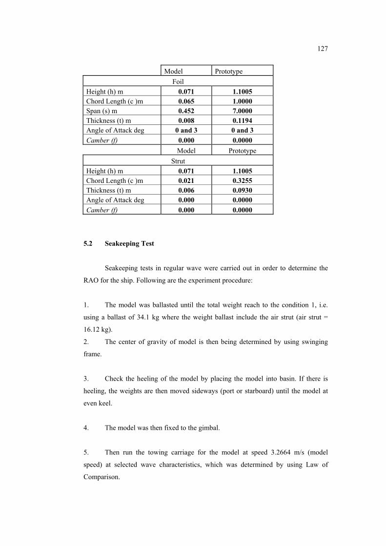
127�

Model Prototype Foil

Height (h) m 0.071 1.1005 Chord Length (c )m 0.065 1.0000 Span (s) m 0.452 7.0000 Thickness (t) m 0.008 0.1194 Angle of Attack deg 0 and 3 0 and 3 Camber (f) 0.000 0.0000

Model Prototype Strut

Height (h) m 0.071 1.1005 Chord Length (c )m 0.021 0.3255 Thickness (t) m 0.006 0.0930 Angle of Attack deg 0.000 0.0000 Camber (f) 0.000 0.0000

5.2 Seakeeping Test

Seakeeping tests in regular wave were carried out in order to determine the

RAO for the ship. Following are the experiment procedure:

1. The model was ballasted until the total weight reach to the condition 1, i.e.

using a ballast of 34.1 kg where the weight ballast include the air strut (air strut =

16.12 kg).

2. The center of gravity of model is then being determined by using swinging

frame.

3. Check the heeling of the model by placing the model into basin. If there is

heeling, the weights are then moved sideways (port or starboard) until the model at

even keel.

4. The model was then fixed to the gimbal.

5. Then run the towing carriage for the model at speed 3.2664 m/s (model

speed) at selected wave characteristics, which was determined by using Law of

Comparison.

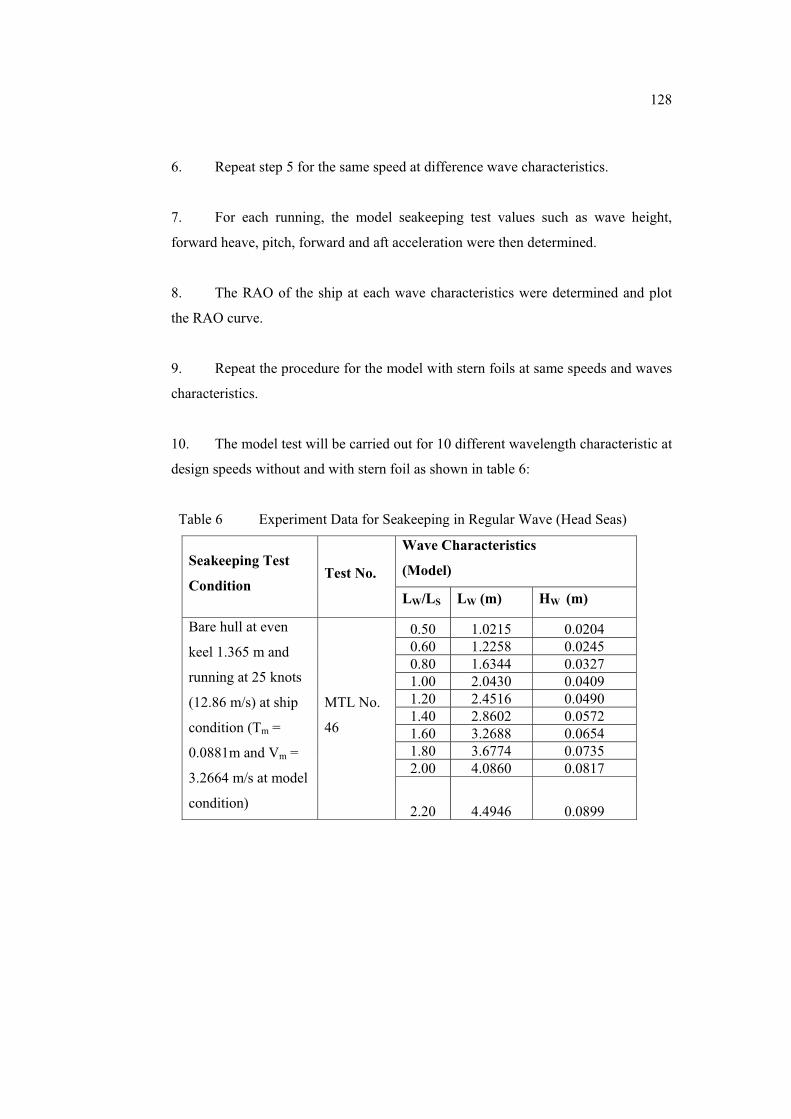
128�

6. Repeat step 5 for the same speed at difference wave characteristics.

7. For each running, the model seakeeping test values such as wave height,

forward heave, pitch, forward and aft acceleration were then determined.

8. The RAO of the ship at each wave characteristics were determined and plot

the RAO curve.

9. Repeat the procedure for the model with stern foils at same speeds and waves

characteristics.

10. The model test will be carried out for 10 different wavelength characteristic at

design speeds without and with stern foil as shown in table 6:

Table 6 Experiment Data for Seakeeping in Regular Wave (Head Seas)

Seakeeping Test

Condition Test No.

Wave Characteristics

(Model)

LW/LS LW (m) HW (m)

Bare hull at even

keel 1.365 m and

running at 25 knots

(12.86 m/s) at ship

condition (Tm =

0.0881m and Vm =

3.2664 m/s at model

condition)

MTL No.

46

0.50 1.0215 0.0204 0.60 1.2258 0.0245 0.80 1.6344 0.0327 1.00 2.0430 0.0409 1.20 2.4516 0.0490 1.40 2.8602 0.0572 1.60 3.2688 0.0654 1.80 3.6774 0.0735 2.00 4.0860 0.0817

2.20 4.4946 0.0899

F

Figure 5 Ship Moddel Body Plaan

1229�

�

�

APPENDIX C

Sample of Resistance Prediction

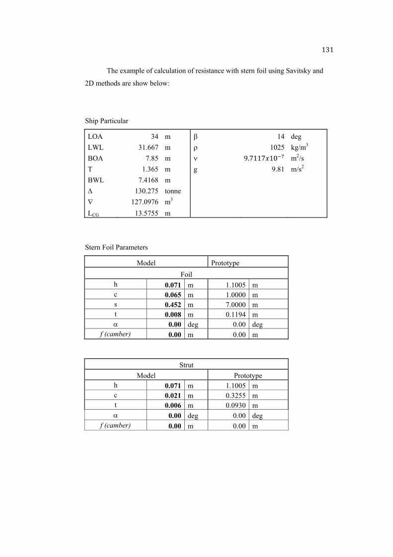
F=F�

�

The example of calculation of resistance with stern foil using Savitsky and

2D methods are show below:

Ship Particular

LOA 34 m � 14 deg LWL 31.667 m � 1025 kg/m3 BOA 7.85 m � ÷>�FF�\FEc� m2/s T 1.365 m g 9.81 m/s2 BWL 7.4168 m � 130.275 tonne � 127.0976 m3 LCG 13.5755 m

Stern Foil Parameters

Model Prototype Foil

h 0.071 m 1.1005 m c 0.065 m 1.0000 m s 0.452 m 7.0000 m t 0.008 m 0.1194 m � 0.00 deg 0.00 deg

f (camber) 0.00 m 0.00 m

Strut Model Prototype

h 0.071 m 1.1005 m c 0.021 m 0.3255 m t 0.006 m 0.0930 m � 0.00 deg 0.00 deg

f (camber) 0.00 m 0.00 m

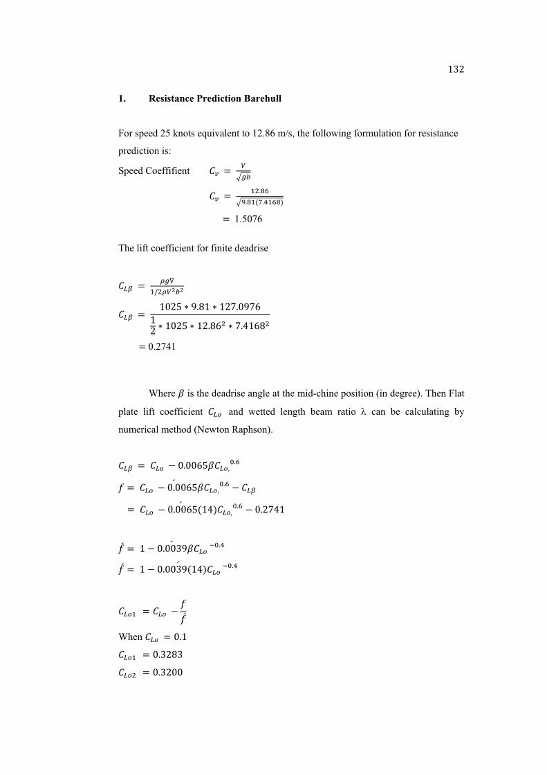
F=G�

�

1. Resistance Prediction Barehull

For speed 25 knots equivalent to 12.86 m/s, the following formulation for resistance

prediction is:

Speed Coeffifient �� A � ��

�� A � DW>øS�ª>øD)�> DSø+ ��A��1.5076

The lift coefficient for finite deadrise

�� A � T�UDVWT�'�'

�� A � FEG? ù ÷>úF ù FG�>E÷�QFG ù FEG? ù FG>úQW ù �>�FQúW

A�0.2741

Where R is the deadrise angle at the mid-chine position (in degree). Then Flat

plate lift coefficient �� and wetted length beam ratio can be calculating by

numerical method (Newton Raphson).

�� A �� P E>EEQ?R��2J>S , A �� P E>EEQ?R��2J>S{ P �� A �� P E>EEQ?)F�+��2J>S{ P E>G��F

,{ A �F P E>EE=÷R��cJ> { ,{ A �F P E>EE=÷)F�+��cJ> {

��D�� A �� P ,,{ When �� A E>F ��D�� A E>=Gú= ��W�� A E>=GEE

F==�

�

��©�� A E>=GEE

Then from Newton Raphson, the value of ��rp

Limit <0.00001

��)�Ñ�+�� A ��© P ��W�� A E>=GEE P E>=GEE ��A E>EE

So the answer for ��rp� E>=GEE

Then for is wetted length beam ratio A £¤¥ and can be determined using Newton

Raphson formulation:

¦��§ P E>�? I ¨ D�>'�¢O'

M eW>©ª« A E

n A �E>�÷G?ûü�¦ P G>=÷M�8n I =>÷E�?�@W�ü�¦ P{ ?>GF�@W�8n

ný A �G>=��?Mü�¦ P �>�ú�8n I =>÷E�?�@W�ü�¦{

D�� A �� P nný When �� A �>E

D� A �>�?Qú

W�� A �>=ú÷ú

©�� A �>=úúF

�� A �>=úúF

Then using Newton Raphson, the value of �rp

Limit <0.00001

þ�� A �� P ©��

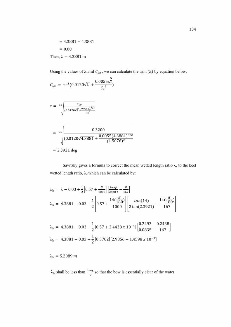
F=��

�

��A �>=úúF P �>=úúF ��A E>EE

Then, A �>=úúF m

Using the values of �ðë� ��, we can calculate the trim (+ by equation below:

�� A � CD>D)E>EFGEH� I E>EE??LM��W +

C A � N�¡�)J>JDWJH�e#>##��LVM¢O'�>�

��A � � E>=GEE)E>EFGEH�>=úúF I E>EE??)�>=úúF+LVM)F>?E�Q+W�>�

��A G>=÷GF deg

Savitsky gives a formula to correct the mean wetted length ratio , to the keel

wetted length ratio, k which can be calculated by:

¬ A � P E>E= I DW E>?� I DJJJ® ][� W ¯°� ± P DS�®

¬ A ��>=úúF P E>E= I FG �E>?� I F�) xFúE+FEEE � � h5i)F�+G éðë)G>=÷GF+ P F�) xFúE+FQ� �

¬ A ��>=úúF P E>E= I FG »E>?� I G>��=ú�\�FEc ¾ ÄE>G�÷=E>Eú=? P E>G�=úFQ� Å

¬ A ��>=úúF P E>E= I FG »E>?�EG¾»G>÷ú?Q P F>�?÷ú�\�FEc©¾

¬ A ?>GEú÷�j

�¬ shall be less than £²³¥ so that the bow is essentially clear of the water.

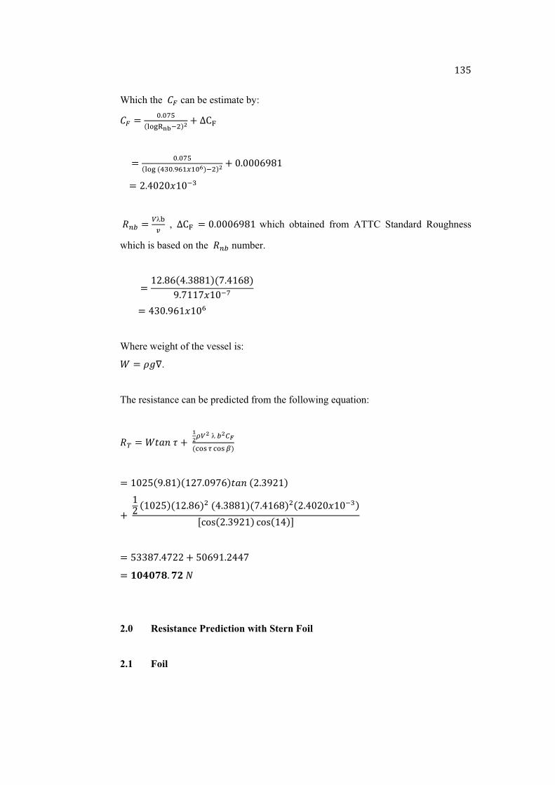
F=?�

�

Which the �� can be estimate by: �� A J>J�K)��·¸cW+' I ��

��A J>J�K)��) ©J>ªSD_DJ�+cW+' I E>EEEQ÷úF ��A G>�EGE\FEc©

�� A �¥� , �� A E>EEEQ÷úF which obtained from ATTC Standard Roughness

which is based on the �� number.

��A FG>úQ)�>=úúF+)�>�FQú+÷>�FF�\FEc� ��A �=E>÷QF\FES

Where weight of the vessel is: � A lnU.

The resistance can be predicted from the following equation:

�� A �h5i�C I��'T�'��'N´)µ�¶ ± µ�¶ + ��A FEG?)÷>úF+)FG�>E÷�Q+h5i�)G>=÷GF+ ��I �FG )FEG?+)FG>úQ+W�)�>=úúF+)�>�FQú+W)G>�EGE\FEc©+»èí)G>=÷GF+ èí)F�+¾

A ?==ú�>��GG I ?EQ÷F>G�� A �� >�M��

2.0 Resistance Prediction with Stern Foil

2.1 Foil

F=Q�

�

The formulation of the viscous resistance on the foil can be expressed as:

�� A X8�

��A FG>úQ)F>E+÷>�FF�\FEc� ��A F>=G=�?\FE�

�� A E>E�?)áonDJ�� P G+W

��A E>E�?)áonDJ)F>=G=�?\FE�+ P G+W

��A G>ú?÷F\FEc©

�� A G��»F I G)hV8+ I QE)hV8+ ¾ ��A G)G>ú?÷F\FEc©+»F I G)E>FF÷�VF>EE+ I QE)E>FF÷�VF>EE+ ¾ ��A �>F?=�\FEc©

The viscous resistance can be calculated as follows:

�� A E>?��lXW( ��A E>?)�>F?=�\FEc©+)FEG?+)FG>úQ+W)F+ ��A ��> û��M

The induced resistance can be described as follows which the foil at zero angle of

attack,

� A É �px8JÊ

��A � )�+")D+$ ��A ú>÷FF?

( A ÞYW�à

��A Þ �Wú>÷FF?à

F=��

�

��A ?>�÷ú?

�� A �x%�)� I G+W

��A �x �E) xFúE+$ ú>÷FF?)ú>÷FF? I G+W

��A �> �

�� A E>?��lXW( ��A �> �

The circulation�� for wave resistance of the foil can be calculated as follow:

�"� P J>K��W") Ü'eJ>WK�'+ A X �% I Wm� $

At zero angle of attack and uncamber foil:

�x)F>E+ P E>?)F>E+�Gx)�)F>EE?+W I E>G?)F>E+W+ A FG>úQ É)E+ I G)E+)F>E+Ê

A �> �

The wave resistance due to the foil can be described as:

.�Ü A X�n�� A FG>úQ�÷>úF)F>FEE?+ ��A =>÷F=÷

�� A T��'�' ��Þ �'´fß'à

��A )FEG?+)÷>úF+)E>E+W)FG>úQ+W ��É cW)©>ªD©ª+'Ê ��A �> �

The spray resistance for foil system as follow:

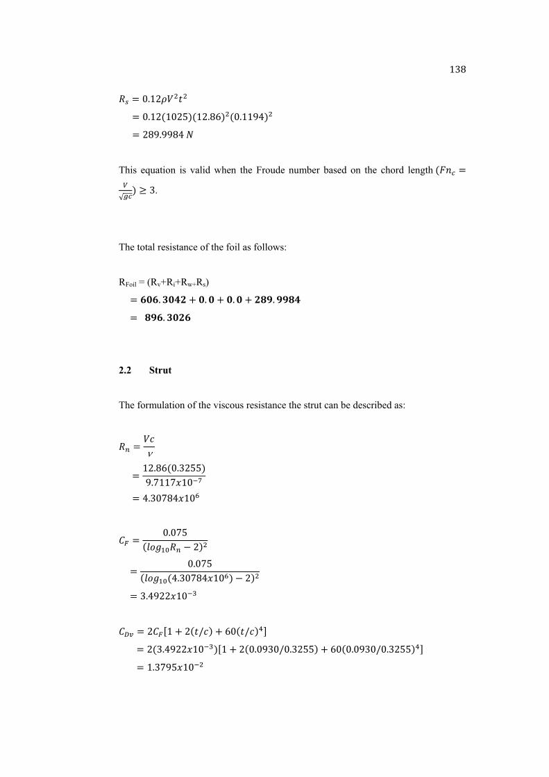
F=ú�

�

�! A E>FGlXWhW ��A E>FG)FEG?+)FG>úQ+W)E>FF÷�+W ��A Gú÷>÷÷ú��

This equation is valid when the Froude number based on the chord length�).i� A�H��+ < =.

The total resistance of the foil as follows:

RFoil = (Rv+Ri+Rw+Rs) ��A ��> û��M I �> � I �> � I M �>�� A �� > û�M�

2.2 Strut

The formulation of the viscous resistance the strut can be described as:

�� A X8�

��A FG>úQ)E>=G??+÷>�FF�\FEc� ��A �>=E�ú�\FES

�� A E>E�?)áonDJ�� P G+W

��A E>E�?)áonDJ)�>=E�ú�\FES+ P G+W

��A =>�÷GG\FEc©

�� A G��»F I G)hV8+ I QE)hV8+ ¾ ��A G)=>�÷GG\FEc©+»F I G)E>E÷=EVE>=G??+ I QE)E>E÷=EVE>=G??+ ¾ ��A F>=�÷?\FEcW

F=÷�

�

The viscous resistance can be calculated as follows: �� A E>?��lXW( ��A E>?)F>=�÷?\FEcW+)FEG?+)FG>úQ+W)E>=G??+ ��A û �>��û�

The induced resistance can be described as follows which the strut at zero angle of

attack. The span of strut is an equivalent to high of the strut.

� A É �px8JÊ

��A � )D>DJJK+")J>©WKK+$ ��A �>=E�G

( A ÞYW�à

��A Þ)F>FEE?+W�>=E�G à

��A E>GúF�

�� A �x%�)� I G+W

��A �x �E) xFúE+$ �>=E�G)�>=E�G I G+W

��A �> �

�� A E>?��lXW( ��A �> �

The wave resistance for strut is considering small when .�� < =>E which in this case .��rp�=>E so that the wave resistance equal to zero.

.�� A X�n8�

F�E�

�

��A FG>úQ�÷>úF)E>=G??+ ��A �>F÷Q�

The spray resistance for strut as follow:

�! A E>FGlXWhW ��A E>FG)FEG?+)FG>úQ+W)E>E÷=E+W ��A F�?>÷=?=��

This equation is valid when the Froude number based on the chord length�).i� A�H��+ < =.

The total resistance of the 2 unit of strut that use as follows:

RStrut = 2(Rv+Ri+Rw+Rs) ��A M)û �>��û� I �> � I �> � I �L>�ûLû+� ��A ��2û> ��

3.0 The Combination Total Resistance

The total resistance for the vessel on planing hull taking account from

resistance on barehull and the foil and strut. The total resistance at speed 25 knots

(12.86 m/s) is:

RT= Rbarehull (vessel)+Rfoil+Rstrut ��A )�� >�M� I ��> û�M� I 2û> ��+ ��A ��2 � >��

APPENDIX D

FORTRAN Programming on Resistance Prediction

142

1.0� FORTRAN�Programming�(Source�Code)��ôõè�õðö�äìíêíéðëì��ð�ó�ðéêèë��æ�� õìð��æå2��2��2�2 2�ìéð2�2!è�2!öêë2�2õ"è2ìó2�2èõ�2ñöð#��õìð��"í2í2íí2éí2"é2é2íé2é"�� "ðõðéìõ�$ê�ìëðöì%FE2&ìí%G2íðñì$ê�ìëðöì%FE�� îõêëé%2'�'��îõêëé%2'ïì�èöì�éè�äìíêíéðëì�ôõì�êéêèë�ç�(�)ó��'��îõêëé%2'�'��îõêëé%2'ô�ìðíì��ëéìõ�*èóõ�+"êî�ôðõéêó�ðõ�,ê�ì��ðöì'��îõêëé%2'�'�� õìð�%2$ê�ìëðöì�� îõêëé%2'�'�� îõêëé%2'*èóõ�+"êî�ôðõéêó�ðõ�,ê�ì��ðöì-'2$ê�ìëðöì�� îõêëé%2'�'��æîìë��ðéð�$ê�ì�$èõ�êëîóé�� ôõêëé%2.*èóõ�,ê�ì��ðöì�êí�.2$ê�ìëðöì�� èîìë�)óëêéAFF2�$ê�ìA$ê�ìëðöì2�íéðéóíA'è��'+�� õìð�)FF2%+��æå�� õìð�)FF2%+�� õìð�)FF2%+�� õìð�)FF2%+�� õìð�)FF2%+� �� õìð�)FF2%+��ìéð�� õìð�)FF2%+�� õìð�)FF2%+�!è�� õìð�)FF2%+�!öêë�

143

� � õìð�)FF2%+�!öð#�� õìð�)FF2%+�� õìð�)FF2%+�õ"è�� õìð�)FF2%+�ìó�� õìð�)FF2%+�"í2"é�� õìð�)FF2%+�í2é�� õìð�)FF2%+�íí2íé�� õìð�)FF2%+�éí2é"�� õìð�)FF2%+�ðë�í2ðë�é�� õìð�)FF2%+�$í2$é�� õìð�)FF2%+��+ðñì�èóéîóé��ðéð�éè�ð�óíìõ�íîìê$êì��$ê�ì��îõêëé%2�''��ôõêëé%2.+ðñì�é"ì��ðéð/�)*V�+.��õìð�%2&ìí��ê$�)&ìí>�0>.&.>èõ>&ìí>�0>.*.+�é"ìë��ôõêëé%2.�ëéìõ�$ê�ì�ëðöì/.��õìð�%2íðñì$ê�ìëðöì�� îõêëé%2''��èîìë�)óëêé�A�FG2$ê�ì�A�íðñì$ê�ìëðöì2�íéðéóíA.óë1ëè�ë.+��õêéì)FG2%+'22222222222222222��ò�ô� ��å å�3222222222222222222'�� õêéì)FG2%+'�'�� õêéì)FG2%+'�ìë�é"�æñìõð��)ö+��A'2�æå�� õêéì)FG2%+'�ìë�é"�ïðéìõ�êëì�)ö+��A'2��õêéì)FG2%+'�õìð�é"�ïðéìõ�êëì�)ö+��A'2��õêéì)FG2%+'�ìîé"�)ö+��A'2�� õêéì)FG2%+'�õðó�"é�)ö+��A'2 �

144

� �� õêéì)FG2%+'�ìð�õêíì�åë��ì�)�ì�+��A'2�ìéð�� õêéì)FG2%+'�èë�>�ìëéìõ��õðñêé&)ö+��A'2�� õêéì)FG2%+'!è�óöì�)ö+��A'2!è�� õêéì)FG2%+'çêë�+"êî�+îìì��)1ëèéí+��A'2!öêë�� õêéì)FG2%+'çð#�+"êî�+îìì��)1ëèéí+��A'2!öð#�� õêéì)FG2%+'�õðñêé&�)öVíG+��A'2�� õêéì)FG2%+'+ìð�ïðéìõ��ìëíêé&)1�Vö=+�A'2õ"è�� õêéì)FG2%+'4êëìöðéê�!ì�èêé&)öGVí+�A'2ìó�� õêéì)FG2%+'�'�� õêéì)FG2%+'� � � ��,èê��+éõóé'��õêéì)FG2%+''�� õêéì)FG2%+')ìê�"é�)ö+��A'2"í2"é��õêéì)FG2%+'�"èõ��ìë�é"�)ö+��A'2í2é��õêéì)FG2%+'+îðë��)ö+��A'2íí2íé��õêéì)FG2%+' "ê1ëìíí��)ö+��A'2éí2é"�� õêéì)FG2%+'åë��ì�è$�åééð1��A'2ðë�í2ðë�é�� õêéì)FG2%+'çð#êöóö��ðö5ìõ��A'2$í2$é�� êíî�ð&�é"ì�êëîóé�èë�é"ì�íõììë�ðë��õêéì�é"ì�êëîóé�èë�ð�óíìõ�íîìê$êì��$ê�ì�� îõêëé%2'222222222��ò�ô� ��å å�3222222222222222222'�� îõêëé%2'�'�� îõêëé%2'�ìë�é"�æñìõð��)ö+��A'2�æå�� îõêëé%2'�ìë�é"�ïðéìõ�êëì�)ö+��A'2��îõêëé%2'�õìð�é"�ïðéìõ�êëì�)ö+��A'2��îõêëé%2'�ìîé"�)ö+��A'2�� îõêëé%2'�õðó�"é�)ö+��A'2 �� îõêëé%2'�ìð�õêíì�åë��ì�)�ì�+��A'2�ìéð�� îõêëé%2'�èë�>�ìëéìõ��õðñêé&)ö+��A'2�� îõêëé%2'!è�óöì�)ö+��A'2!è�� îõêëé%2'çêë�+"êî�+îìì��)1ëèéí+��A'2!öêë�

145

� � �îõêëé%2'çð#�+"êî�+îìì��)1ëèéí+��A'2!öð#�� îõêëé%2'�õðñêé&�)öVíG+��A'2�� îõêëé%2'+ìð�ïðéìõ��ìëíêé&)1�Vö=+�A'2õ"è�� îõêëé%2'4êëìöðéê�!ì�èêé&)öGVí+�A'2ìó�� îõêëé%2'�'�� îõêëé%2'� � � ��,èê��+éõóé'��îõêëé%2''��îõêëé%2')ìê�"é�)ö+��A'2"í2"é��îõêëé%2'�"èõ��ìë�é"�)ö+��A'2í2é��îõêëé%2'+îðë��)ö+��A'2íí2íé��îõêëé%2' "ê1ëìíí��)ö+��A'2éí2é"�� îõêëé%2'åë��ì�è$�åééð1��A'2ðë�í2ðë�é�� îõêëé%2'çð#êöóö��ðö5ìõ��A'2$í2$é��îõêëé%2'(((((((((((((((((((((((((((((((((((((((((((((((((((('��ð�ó�ðéêèë�ôõèì�óõì��õêéì)FG2%+'��å��å òæ�ä�+�� 33333333333333'�� õêéì)FG2%+�''�� ê$�)&ìí>�0>.&.>èõ>&ìí>�0>.*.+�é"ìë�GEE� ��!íA!öêë�� îõêëé�Fú2!í�� õêéì)FG2Fú+�!í��Fú��$èõöðé)''2'�!íA'2�62,�>G+�� ñA)!öêë%E>?F��+V)�%��+%%E>?��îõêëé�?2�ñ��õêéì)FG2?+�ñ��

146

?��$èõöðé)''2'��ñA'2?62,�>�+�� 5A)õ"è%�%!è�+V)E>?%õ"è%)!öêë%E>?F��+%%G%)��+%%G+��îõêëé�Q2��5�� õêéì)FG2Q+��5�� Q��$èõöðé)''2'��5A'2=62,�>�+�� AE>F�FGE� ��ð��$)62�2��2�ñ2�+�� ð��$�èé)*2�2��2�ñ2�+�� FA�(6V*�� )A�F(�� ê$)å�+))+>��>F>E�(EQ+�é"ìë�� A�F�� îõêëé�=E2�� õêéì)FG2=E+��=E� ��$èõöðé�)''2'��A'2Q62,�>�+�� ì�íì�� A�F� � � � �� èéè�FGE�� ìë��ê$�� èAE>F�F=E� ��ð��1)å2�è2�ìéð2��5+�� ð��1�èé)�2�ìéð2�è+�

147

� ��èFA�è(åV�� A�èF(�è�� ê$�)å�+)�+>��>F>�(E�+�é"ìë�� èA�èF�� îõêëé�=F2�è�� õêéì)FG2=F+��è��=F� ��$èõöðé�)''2'��èA'2=62,�>�+�� ì�íì�� èA�èF�� èéè�F=E�� ìë��ê$�� õêöA)�è%�ñ%%GV)E>EFG%�ñ%%G%)�+%%E>?IE>EE??%)�+%%G>?++%%E>÷F�� îõêëé��2 õêö�� õêéì)FG2�+� õêö�� $èõöðé)''2'� õêöA'2=62,�>�+�� ð��äð�í)äð�êðë2ôò+�èõ�A�(E>E=I)E>?%)E>?�I)äð�êðë%�ìéð+VFEEE+%) ðë�)�ìéð+VG% ðë�) õêö+()äð�êðë%�ìéð+VFQ�++�� îõêëé�ú2èõ��õêéì)FG2ú+�èõ��ú��$èõöðé)''2'�èõ�A'2=62,�>�+��

148

��äëA))!öêë%E>?F��+%��%�+Vìó�� ,A)E>E�?+V)�è�FE)äë+(G+%%G�� $AQ>÷úFE�(E�� ä,A)õ"è%)!öêë%E>?F��+%%G%)�+%��%%G%)�,I�$++V)G%�èí�) õêö+%�èí�)�ìéð++�� îõêëé%2'ä,A'2ä,�� äïAõ"è%�%!è�% ðë�) õêö+�� îõêëé%2'äïA'2äï�� ,ë"íA)!öêë%E>?F��+V)�%"í+%%E>?�� îõêëé%2',ë"íA'2�,ë"í�� äëíA)!öêë%E>?F��+%íVìó�� îõêëé%2'äëíA'2�äëí�� $íAE>E�?V)�è�FE)äëí+(G+%%G�� îõêëé%2'�$íA'2��$í�� ,ëíA)!öêë%E>?F��+V)�%í+%%E>?�� îõêëé%2',ëíA'2�,ëí�� åäA)�%íí+V=>F�FQ%í�� îõêëé%2'åäA'2�åä�� åAíí%%GVåä�� îõêëé%2'åA'2�å�� ñíAG%�$í%)FIG%)éíVí+IQE%)éíVí+%%�+�� îõêëé%2'�ñíA'2��ñí�� äñíA�ñí%E>?%õ"è%)!öêë%E>?F��+%%G%í�� îõêëé%2'äñíA'2�äñí�� õð�A=>F�FQVFúE��

149

� � �êíA�%=>F�FQ%õð�%ðë�í%åäV)åäIG+%%G�� äêíAE>?%�êí%õ"è%)!öêë%E>?F��+%%G%å�� îõêëé%2'äêíA'2�äêí�� êõA))!öêë%E>?F��+%í%õð�%ðë�íIG%$í%)!öêë%E>?F��++%)ú%=>F�FQ%%G%)"í+%%GIE>?%=>F�FQ%%G%)í+%%G+V)F(E>?%í+�� ä�íA)õ"è%�%�êõ%%GV)!öêë%E>?F��+%%G+%ì#î)(GV,ë"í%%G+�� îõêëé%2'ä�íA'2�ä�í�� äíéAE>FG%õ"è%)!öêë%E>?F��+%%G%)éí+%%G�� îõêëé%2'äíéA'2�äíé�� äé$èê�AäñíIäêíIä�íIäíé�� îõêëé%2'äé$èê�A'2�äé$èê�� ,ë"éA)!öêë%E>?F��+V)�%"é+%%E>?�� îõêëé%2',ë"éA'2�,ë"é�� äëéA)!öêë%E>?F��+%éVìó�� îõêëé%2'äëéA'2�äëé�� $éAE>E�?V)�è�FE)äëé+(G+%%G�� îõêëé%2'�$éA'2��$é�� ,ëéA)!öêë%E>?F��+V)�%é+%%E>?�� îõêëé%2',ëéA'2�,ëé�� åäA)�%"é+V)=>F�FQ%é+�� îõêëé%2'åäA'2�åä�� åA"é%%GVåä�� îõêëé%2'åA'2�å�� ñéAG%�$é%)FIG%)é"Vé+IQE%)é"Vé+%%�+�� îõêëé%2'�ñéA'2��ñé�

150

� � äñéA�ñé%E>?%õ"è%)!öêë%E>?F��+%%G%é�� îõêëé%2'äñéA'2�äñé�� õð�AîêVFúE�� êéA�%=>F�FQ%õð�%ðë�é%åäV)åäIG+%%G�� äêéAE>?%�êé%õ"è%)!öêë%E>?F��+%%G%å�� îõêëé%2'äêéA'2�äêé�� äíéõAE>FG%õ"è%)!öêë%E>?F��+%%G%)é"+%%G�� îõêëé%2'äíéA'2�äíé�� äéíéõóéAG%)äñéIäêéIäíéõ+�� îõêëé%2'äéíéõóéA'2�äéíéõóé�� äé"ó��AäïIä,Iäé,èê�Iäé+éõóé�� îõêëé�=G2äé"ó�� õêéì)FG2=G+�äé"ó��=G� � $èõöðé)''2'�äé"ó��A'2F62,FE>G+�� õêéì)FG2%+�� õêéì)FG2%+�� îõêëé%2''�� îõêëé%2''�� ê$�)!öêë>�é>!öð#+�é"ìë�� !öêëA!öêëIF�� èéè�GEE�� ìë��ê$�� ìë��ê$�

151

� � �ôõêëé%2.�ðéð�íðñì��êë�.2íðñì$ê�ìëðöì�� ì�íì�� îõêëé%2'�ðéð��èé�íðñì�'�� èíì�)FG+�� ìë��ê$�� ë��úúúúúúúúúúúúúúúúúúúúúúúúúúúúúúúúúúúúúúúúúúúúúúúúúúúúúúúúúúúúúúú�+ó5õèóéêëì�$)62�2��2�ñ2�+�6AE>�÷G?%��%�%%=(G>=÷%�%�%%GI=>÷E?%��%�ñ%%G%�(?>GF%�%�ñ%%G�õìéóõë�ìë��AAAAAAAAAAAAAAAAAAAAAAAAAAAAAAAAAAAAAAAAAAAAAAA�� +ó5õèóéêëì�$�èé)*2�2��2�ñ2�+�� ê$�)�>�0>E>E+�é"ìë�� *A=>÷E�?%�ñ%%G%�� õìéóõë�� ì�íì�� *AG>=��?%��%�%%G(�>�ú%�%�I=>÷E?%��%�ñ%%G�� ìë��ê$�� õìéóõë�� ìë��AAAAAAAAAAAAAAAAAAAAAAAAAAAAAAAAAAAAAAAAAAAAAAA��+ó5õèóéêëì�1)å2�è2�ìéð2��5+��åA�è(E>EEQ?%�ìéð%�è%%)E>Q+(��5�� õìéóõë�� ìë��AAAAAAAAAAAAAAAAAAAAAAAAAAAAAAAAAAAAAAAAAAAAAAA�� +ó5õèóéêëì�1�èé)�2�ìéð2�è+�� ê$)�è>�0>E>E+�é"ìë�� AF�

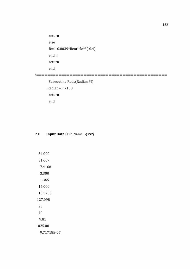
152

� ��õìéóõë�� ì�íì�� AF(E>EE=÷%�ìéð%�è%%)(E>�+�� ìë��ê$�� õìéóõë�� ìë��AAAAAAAAAAAAAAAAAAAAAAAAAAAAAAAAAAAAAAAAAAAAAAA�� +ó5õèóéêëì�äð�í)äð�êðë2ôò+��äð�êðëAôòVFúE�� õìéóõë�� ìë��2.0� Input�Data�7,ê�ì��ðöì�-�q.txt)��=�>EEE��=F>QQ��>�FQú��=>=EE��F>=Q?��F�>EEE��F=>?�??��FG�>E÷ú��G=��E��÷>úF��FEG?>EE��÷>�F�Fú�(E��

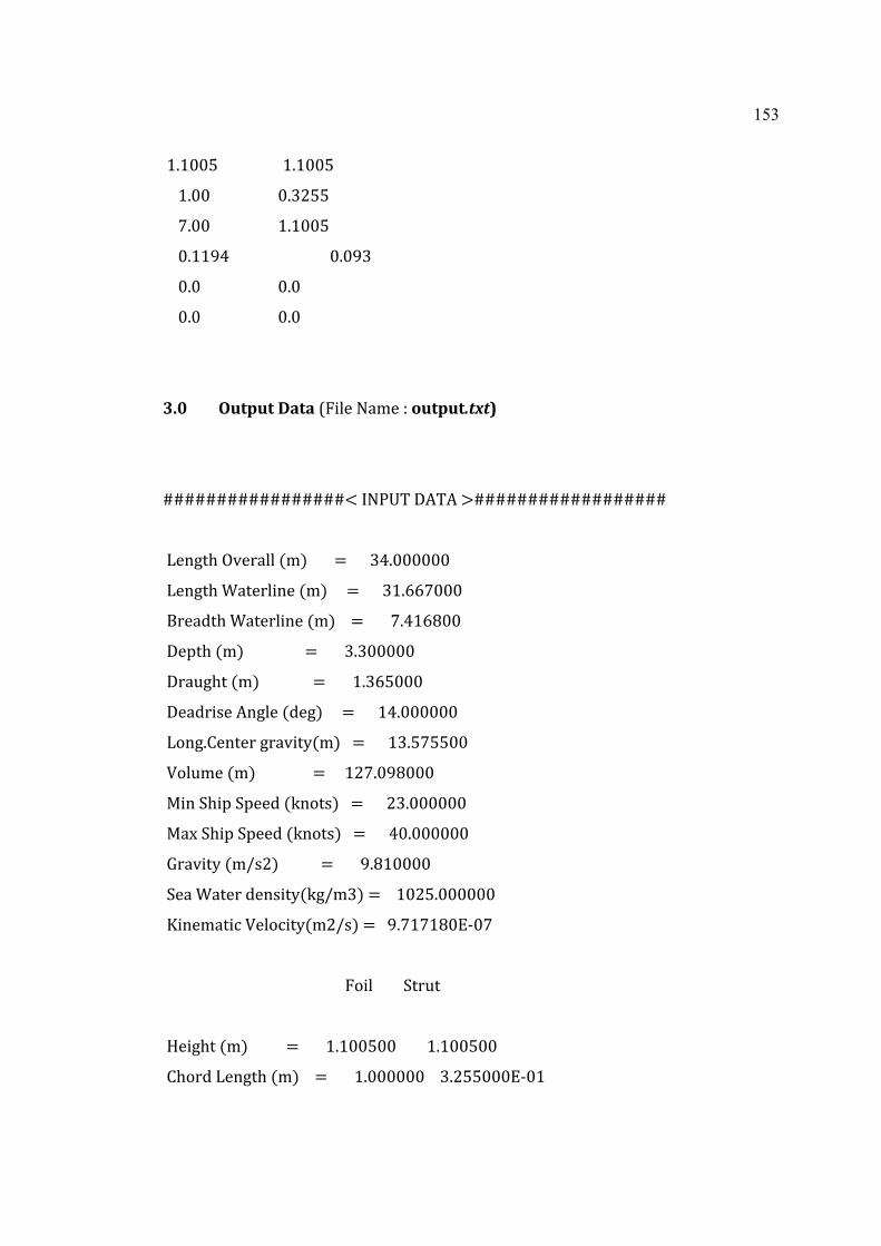
153

�F>FEE?��F>FEE?��F>EE�� E>=G??��>EE�� F>FEE?��E>FF÷�� E>E÷=��E>E� � ��E>E��E>E� �� E>E��3.0� �Output�Data�7,ê�ì��ðöì�-�output.txt)��22222222222222222��ò�ô� ��å å�3222222222222222222��ìë�é"�æñìõð��)ö+��A��=�>EEEEEE��ìë�é"�ïðéìõ�êëì�)ö+��A��=F>QQ�EEE��õìð�é"�ïðéìõ�êëì�)ö+��A��>�FQúEE��ìîé"�)ö+��A��=>=EEEEE��õðó�"é�)ö+��A��F>=Q?EEE��ìð�õêíì�åë��ì�)�ì�+��A��F�>EEEEEE��èë�>�ìëéìõ��õðñêé&)ö+��A��F=>?�??EE��!è�óöì�)ö+��A��FG�>E÷úEEE��çêë�+"êî�+îìì��)1ëèéí+��A��G=>EEEEEE��çð#�+"êî�+îìì��)1ëèéí+��A��E>EEEEEE��õðñêé&�)öVíG+��A��÷>úFEEEE��+ìð�ïðéìõ��ìëíêé&)1�Vö=+�A��FEG?>EEEEEE��4êëìöðéê�!ì�èêé&)öGVí+�A��÷>�F�FúE�(E�� ,èê��+éõóé��)ìê�"é�)ö+��A��F>FEE?EE��F>FEE?EE��"èõ��ìë�é"�)ö+��A��F>EEEEEE��=>G??EEE�(EF�

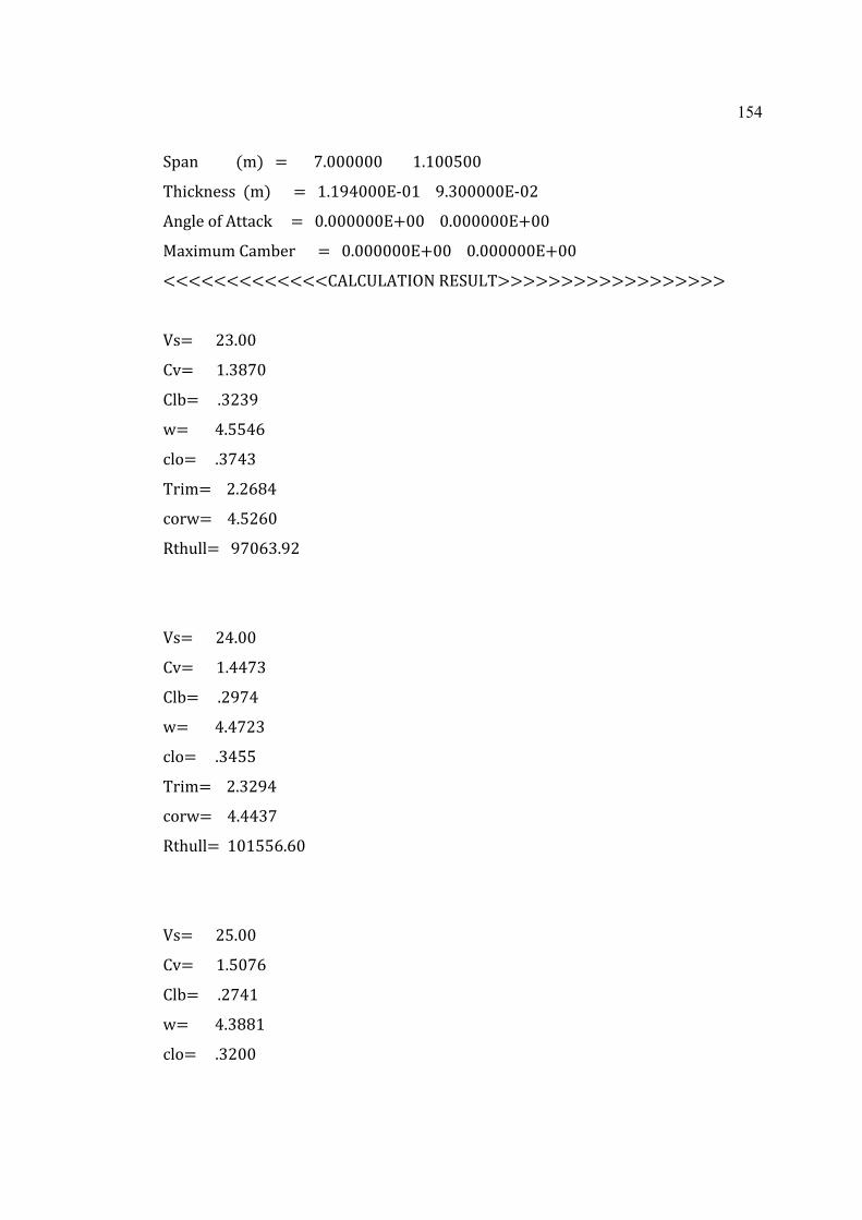
154

�+îðë��)ö+��A��>EEEEEE��F>FEE?EE�� "ê1ëìíí��)ö+��A��F>F÷�EEE�(EF��÷>=EEEEE�(EG��åë��ì�è$�åééð1��A��E>EEEEEE�IEE��E>EEEEEE�IEE��çð#êöóö��ðö5ìõ��A��E>EEEEEE�IEE��E>EEEEEE�IEE��å��å òæ��ä�+�� 333333333333333333��!íA��G=>EE��ñA��F>=ú�E��5A��>=G=÷��A��>??�Q��èA��>=��=�� õêöA��G>GQú��èõ�A��>?GQE��äé"ó��A��÷�EQ=>÷G��!íA��G�>EE��ñA��F>��=��5A��>G÷��A��>��G=��èA��>=�??�� õêöA��G>=G÷��èõ�A��>��=��äé"ó��A��FEF??Q>QE��!íA��G?>EE��ñA��F>?E�Q��5A��>G��F��A��>=úúF��èA��>=GEE�

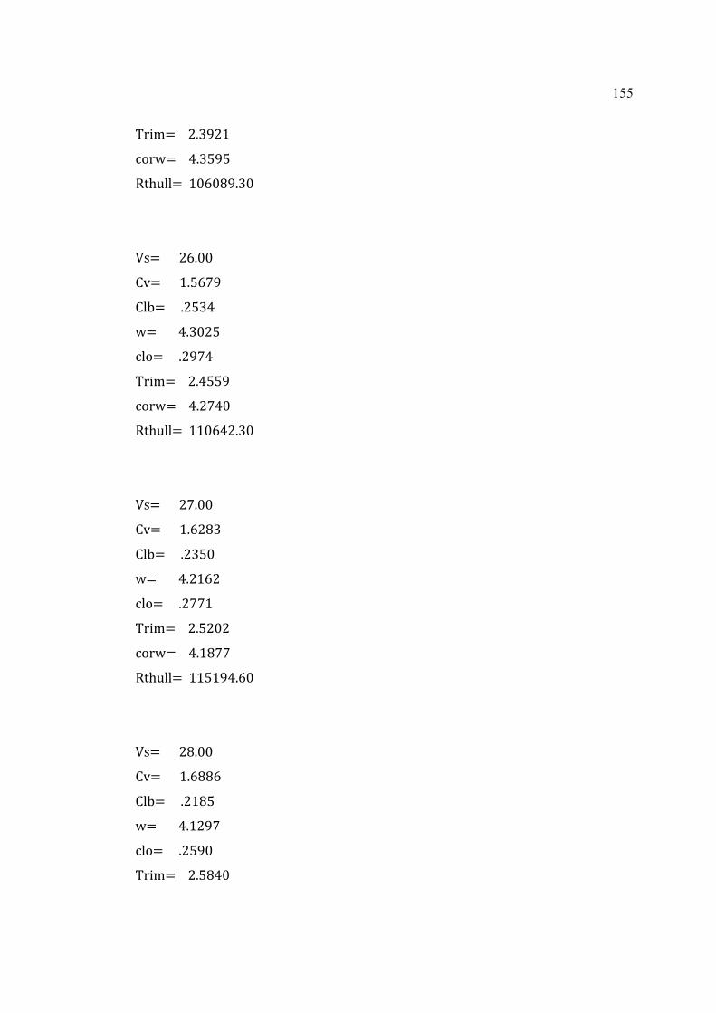
155

� õêöA��G>=÷GF��èõ�A��>=?÷?��äé"ó��A��FEQEú÷>=E��!íA��GQ>EE��ñA��F>?Q�÷��5A��>G?=��A��>=EG?��èA��>G÷�� õêöA��G>�??÷��èõ�A��>G��E��äé"ó��A��FFEQ�G>=E��!íA��G�>EE��ñA��F>QGú=��5A��>G=?E��A��>GFQG��èA��>G��F�� õêöA��G>?GEG��èõ�A��>Fú��äé"ó��A��FF?F÷�>QE��!íA��Gú>EE��ñA��F>QúúQ��5A��>GFú?��A��>FG÷��èA��>G?÷E�� õêöA��G>?ú�E�

156

�èõ�A��>FEF=��äé"ó��A��FF÷�G?>EE��!íA��G÷>EE��ñA��F>��ú÷��5A��>GE=��A��>E�=ú��èA��>G�GQ�� õêöA��G>Q�Q��èõ�A��>EF?��äé"ó��A��FG�GFG>?E��!íA��=E>EE��ñA��F>úE÷G��5A��>F÷E��A��=>÷?÷F��èA��>GG�ú�� õêöA��G>�EQ��èõ�A��=>÷=E��äé"ó��A��FGúQ=Q>÷E��!íA��=F>EE��ñA��F>úQ÷?��5A��>F�ú=��A��=>ú�QG��èA��>GF�� õêöA��G>�QGú��èõ�A��=>ú��÷�

157

�äé"ó��A��F=G÷úE>=E��!íA��=G>EE��ñA��F>÷G÷ú��5A��>FQ�=��A��=>�÷?ú��èA��>GEGG�� õêöA��G>úF�ú��èõ�A��=>�Q�Q��äé"ó��A��F=�GG�>?E��!íA��==>EE��ñA��F>÷÷EF��5A��>F?�=��A��=>�Fú?��èA��>F÷FE�� õêöA��G>úQF=��èõ�A��=>Q÷E=��äé"ó��A��F�F=Q�>QE��!íA��=�>EE��ñA��G>E?E��5A��>F�úG��A��=>Q��Q��èA��>FúEú�� õêöA��G>÷EFQ��èõ�A��=>QFQ��äé"ó��A��F�?=÷=>÷E�

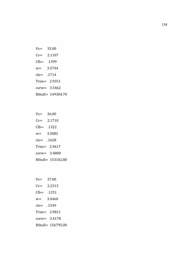
158

��!íA��=?>EE��ñA��G>FFE��5A��>F=÷÷��A��=>?��èA��>F�F�� õêöA��G>÷=?F��èõ�A��=>?�QG��äé"ó��A��F�÷=E�>�E��!íA��=Q>EE��ñA��G>F�FE��5A��>F=GG��A��=>?EúG��èA��>FQGú�� õêöA��G>÷QF��èõ�A��=>�úEE��äé"ó��A��F?=FEG>úE��!íA��=�>EE��ñA��G>G=F=��5A��>FG?F��A��=>��QE��èA��>F?�÷�� õêöA��G>÷úFF��èõ�A��=>�F�ú��äé"ó��A��F?Q�÷?>EE��

159

�!íA��=ú>EE��ñA��G>G÷FQ��5A��>FFúQ��A��=>=ú�ú��èA��>F��?�� õêöA��G>÷÷=?��èõ�A��=>=?÷Q��äé"ó��A��FQE=÷F>QE��!íA��=÷>EE��ñA��G>=?F÷��5A��>FFGQ��A��=>===?��èA��>F�E�� õêöA��G>÷÷÷F��èõ�A��=>=E?=��äé"ó��A��FQ=÷E?>�E��!íA��E>EE��ñA��G>�FGG��5A��>FE�F��A��=>Gú=E��èA��>F=�� õêöA��G>÷÷ú��èõ�A��=>G?�ú��äé"ó��A��FQ�=?E>úE��

APPENDIX E

Offset Table 130.275 Tonnes High Speed Craft

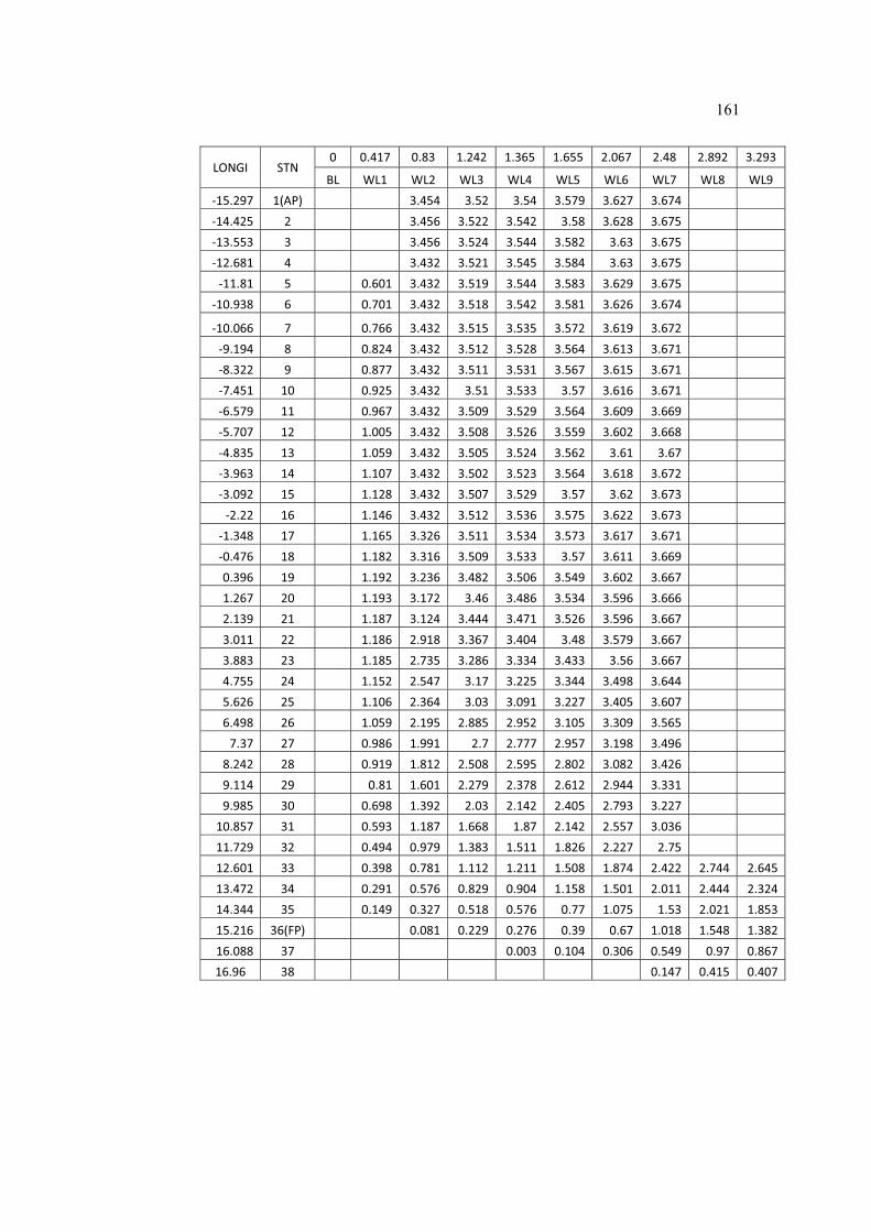
161

LONGI� STN�0� 0.417� 0.83� 1.242� 1.365� 1.655� 2.067� 2.48� 2.892� 3.293�

BL� WL1� WL2� WL3� WL4� WL5� WL6� WL7� WL8� WL9�

�15.297� 1(AP)� �� 3.454� 3.52� 3.54� 3.579� 3.627� 3.674� ��

�14.425� 2� �� 3.456� 3.522� 3.542� 3.58� 3.628� 3.675� ��

�13.553� 3� �� 3.456� 3.524� 3.544� 3.582� 3.63� 3.675� ��

�12.681� 4� �� 3.432� 3.521� 3.545� 3.584� 3.63� 3.675� ��

�11.81� 5� �� 0.601� 3.432� 3.519� 3.544� 3.583� 3.629� 3.675� ��

�10.938� 6� �� 0.701� 3.432� 3.518� 3.542� 3.581� 3.626� 3.674� ��

�10.066� 7� �� 0.766� 3.432� 3.515� 3.535� 3.572� 3.619� 3.672� ��

�9.194� 8� �� 0.824� 3.432� 3.512� 3.528� 3.564� 3.613� 3.671� ��

�8.322� 9� �� 0.877� 3.432� 3.511� 3.531� 3.567� 3.615� 3.671� ��

�7.451� 10� �� 0.925� 3.432� 3.51� 3.533� 3.57� 3.616� 3.671� ��

�6.579� 11� �� 0.967� 3.432� 3.509� 3.529� 3.564� 3.609� 3.669� ��

�5.707� 12� �� 1.005� 3.432� 3.508� 3.526� 3.559� 3.602� 3.668� ��

�4.835� 13� �� 1.059� 3.432� 3.505� 3.524� 3.562� 3.61� 3.67� ��

�3.963� 14� �� 1.107� 3.432� 3.502� 3.523� 3.564� 3.618� 3.672� ��

�3.092� 15� �� 1.128� 3.432� 3.507� 3.529� 3.57� 3.62� 3.673� ��

�2.22� 16� �� 1.146� 3.432� 3.512� 3.536� 3.575� 3.622� 3.673� ��

�1.348� 17� �� 1.165� 3.326� 3.511� 3.534� 3.573� 3.617� 3.671� ��

�0.476� 18� �� 1.182� 3.316� 3.509� 3.533� 3.57� 3.611� 3.669� ��

0.396� 19� �� 1.192� 3.236� 3.482� 3.506� 3.549� 3.602� 3.667� ��

1.267� 20� �� 1.193� 3.172� 3.46� 3.486� 3.534� 3.596� 3.666� ��

2.139� 21� �� 1.187� 3.124� 3.444� 3.471� 3.526� 3.596� 3.667� ��

3.011� 22� �� 1.186� 2.918� 3.367� 3.404� 3.48� 3.579� 3.667� ��

3.883� 23� �� 1.185� 2.735� 3.286� 3.334� 3.433� 3.56� 3.667� ��

4.755� 24� �� 1.152� 2.547� 3.17� 3.225� 3.344� 3.498� 3.644� ��

5.626� 25� �� 1.106� 2.364� 3.03� 3.091� 3.227� 3.405� 3.607� ��

6.498� 26� �� 1.059� 2.195� 2.885� 2.952� 3.105� 3.309� 3.565� ��

7.37� 27� �� 0.986� 1.991� 2.7� 2.777� 2.957� 3.198� 3.496� ��

8.242� 28� �� 0.919� 1.812� 2.508� 2.595� 2.802� 3.082� 3.426� ��

9.114� 29� �� 0.81� 1.601� 2.279� 2.378� 2.612� 2.944� 3.331� ��

9.985� 30� �� 0.698� 1.392� 2.03� 2.142� 2.405� 2.793� 3.227� ��

10.857� 31� �� 0.593� 1.187� 1.668� 1.87� 2.142� 2.557� 3.036� ��

11.729� 32� �� 0.494� 0.979� 1.383� 1.511� 1.826� 2.227� 2.75� ��

12.601� 33� �� 0.398� 0.781� 1.112� 1.211� 1.508� 1.874� 2.422� 2.744� 2.645�

13.472� 34� �� 0.291� 0.576� 0.829� 0.904� 1.158� 1.501� 2.011� 2.444� 2.324�

14.344� 35� �� 0.149� 0.327� 0.518� 0.576� 0.77� 1.075� 1.53� 2.021� 1.853�

15.216� 36(FP)� �� 0.081� 0.229� 0.276� 0.39� 0.67� 1.018� 1.548� 1.382�

16.088� 37� �� 0.003� 0.104� 0.306� 0.549� 0.97� 0.867�

16.96� 38� �� 0.147� 0.415� 0.407�

ii performance prediction for high speed craft anuar … · kapal dengan foil buritan atau...

Documents