1

IES <Virtual Environment> Live e-training

Trainee notes

ApacheHVAC (Version 6.4) Session B

SI units

Introduction In Session A you were shown the basics of creating HVAC plant and control networks for a building using IES’s ApacheHVAC tool. You were shown how to create simple networks for subsequent use by ApacheSim, IES’s dynamic thermal simulation module. In this session (Session B) you will be shown how to create more complex HVAC networks and controls. You will perform ApacheSim dynamic simulations using these networks and you will also look at relevant results within Vista, IES’s results viewer. You will create the HVAC networks for a building model previously created using ModelIT, where you have also set the site location data using the APlocate utility. Constructions and thermal data (internal gains and air exchanges) have also been previously assigned using the Apache software. Attendees of these sessions are assumed to have had previous training in (or be competent with) ModelIT, SunCast, ApacheSim and MacroFlo. The trainer will show you how to perform various functions as shown in the following pages, and images are included to assist you in following the trainer as the session proceeds, and to act as a memory jogger after the session. For more detailed help you can use the Help menu within the specific IES application, and also you can refer to the product manuals installed with the IES software.

2

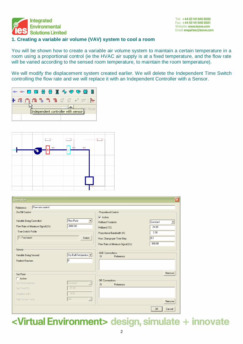
1. Creating a variable air volume (VAV) system to cool a room You will be shown how to create a variable air volume system to maintain a certain temperature in a room using a proportional control (ie the HVAC air supply is at a fixed temperature, and the flow rate will be varied according to the sensed room temperature, to maintain the room temperature). We will modify the displacement system created earlier. We will delete the Independent Time Switch controlling the flow rate and we will replace it with an Independent Controller with a Sensor.

3

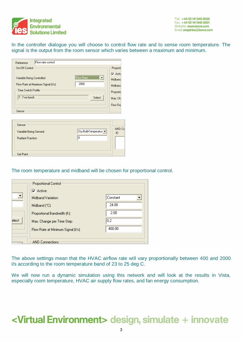
In the controller dialogue you will choose to control flow rate and to sense room temperature. The signal is the output from the room sensor which varies between a maximum and minimum.

The room temperature and midband will be chosen for proportional control.

The above settings mean that the HVAC airflow rate will vary proportionally between 400 and 2000 l/s according to the room temperature band of 23 to 25 deg C. We will now run a dynamic simulation using this network and will look at the results in Vista, especially room temperature, HVAC air supply flow rates, and fan energy consumption.

4

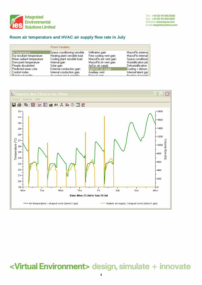
Room air temperature and HVAC air supply flow rate in July

5

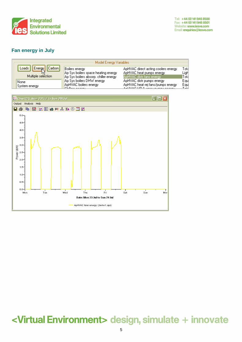
Fan energy in July

6

Annual fan energy consumption

7

Set Point control Instead of (or as well as) using Proportional Control when using an Independent Controller with a Sensor, you may wish to use Set Point (on-off) control. In the previous example the HVAC airflow rate varied proportionally between 400 and 2000 l/s according to the room temperature band of 21 to 23 deg C. . In the example below, Set Point control is employed instead of proportional control, using a set point and a deadband. In the settings below for a cooling example, the flow rate will be either 2000 l/s or zero depending on the temperature of the room. The High Sensor Input setting of ‘ON’ means that the flow rate will be 2000 l/s if the room is warm and zero if the room is cold (note that a High Sensor Input setting of ‘OFF’ would mean that the flow rate will be zero if the room is warm and 2000 l/s if the room is cold).

8

In the example below, Set Point control is employed as well as proportional control. An application of this is a fan in a fan-coil unit with a VSD that can vary its speed between 100% and 20% (via proportional control), but needs to shut off completely when no cooling is demanded as the temperature drops a bit lower (eg below 21 deg C).

9

2. Creating a constant air volume (CAV) system to cool a room You will be shown how to create a constant air volume system to maintain a certain temperature in a room using a proportional control (ie the HVAC air supply is at a fixed flow rate, and the HVAC supply air temperature will be varied according to the sensed room temperature, to maintain the room temperature). We will modify the VAV system created earlier. We will use an Independent Time Switch to fix the flow rate in the system, and an Independent Controller with a Sensor to control the output of the cooling coil according to the room temperature.

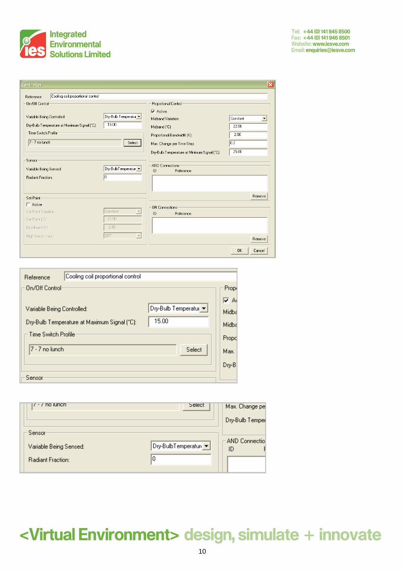
10

11

The above settings mean that the cooling coil output (the off-coil temperature) will vary proportionally between a maximum of 25 deg C and a minimum of 15 deg C (subject to the coil capacity, flow rate, contact factor and the air temperature before the coil) according to the room temperature band of 21 to 23 deg C. We will now run a dynamic simulation using this network and will look at the results in Vista, especially room temperature, coil loads and chiller energy consumption. Room air temperature in August

12

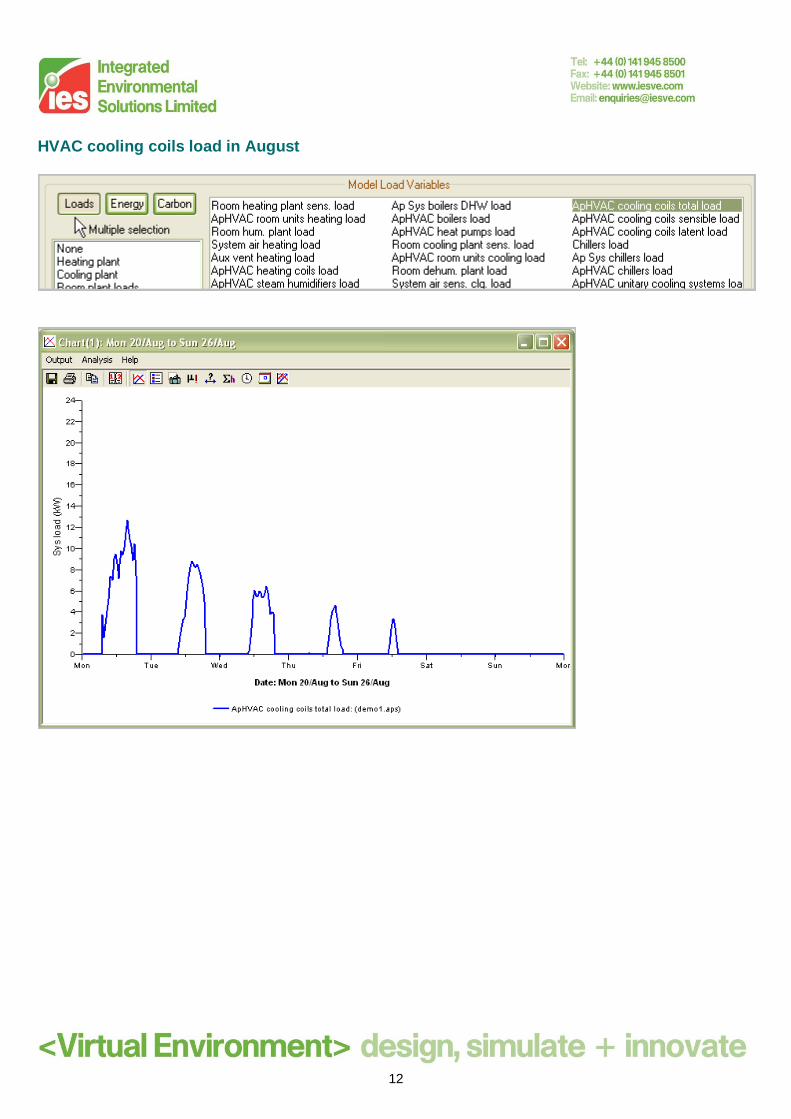
HVAC cooling coils load in August

13

Annual chiller energy consumption

14

3. Creating a fancoil system We will next create a fancoil system for a room to provide cooling and heating by varying the output of both the heating coil and the cooling coil in the unit. You will be shown how to place junctions in the HVAC schematic. There will be two sets of coils. One set will supply fresh air into the building at 19 deg C, and the other set will be in the fancoil unit in the room. Fresh air supply

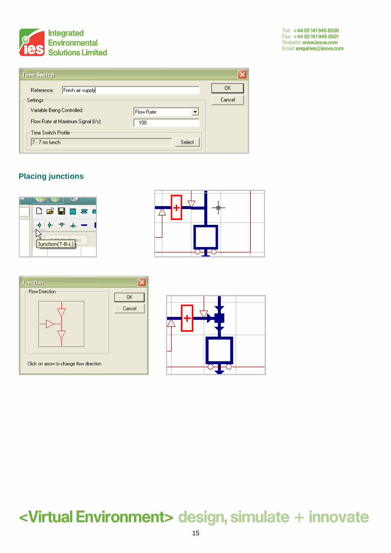
15

Placing junctions

16

The fancoil unit

Fancoil flow rate

17

Fancoil controllers We will use Independent Controllers with Sensors such that either the heating coil or cooling coil in the fancoil unit will operate proportionally depending on the room temperature. The cooling coil will operate if the room temperature is in the band 23 to 25 deg C. The heating coil will operate if the room temperature is in the band 19 to 21 deg C. The Temperature at Maximum Signal and Temperature at Minimum Signal for both coils are set to prevent both coils operating simultaneously (in this example, the temperatures for the cooling control are 1 deg C higher than the corresponding temperatures for the heating coil). Fancoil cooling coil controller

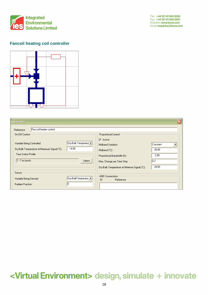
18

Fancoil heating coil controller

19

We will now run a dynamic simulation using this network and will look at the results in Vista, especially room temperature, HVAC air flow rate, coil loads, annual HVAC system energy consumption and annual system CO2 emissions.

20

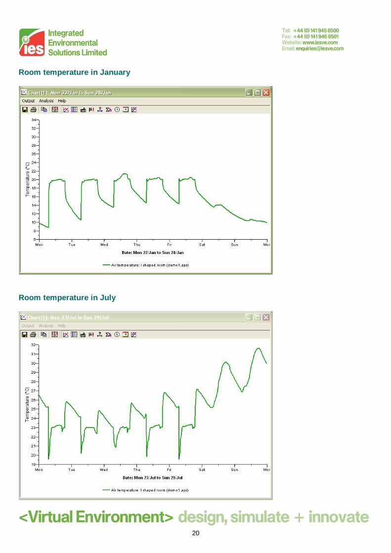
Room temperature in January

Room temperature in July

21

Room HVAC air supply flow rate

22

Heating and cooling coil loads for a whole year

23

Annual HVAC system energy consumption

You will see that in this example the total system energy consumption is the sum of the boilers, chillers, fans and pumps energy consumption.

24

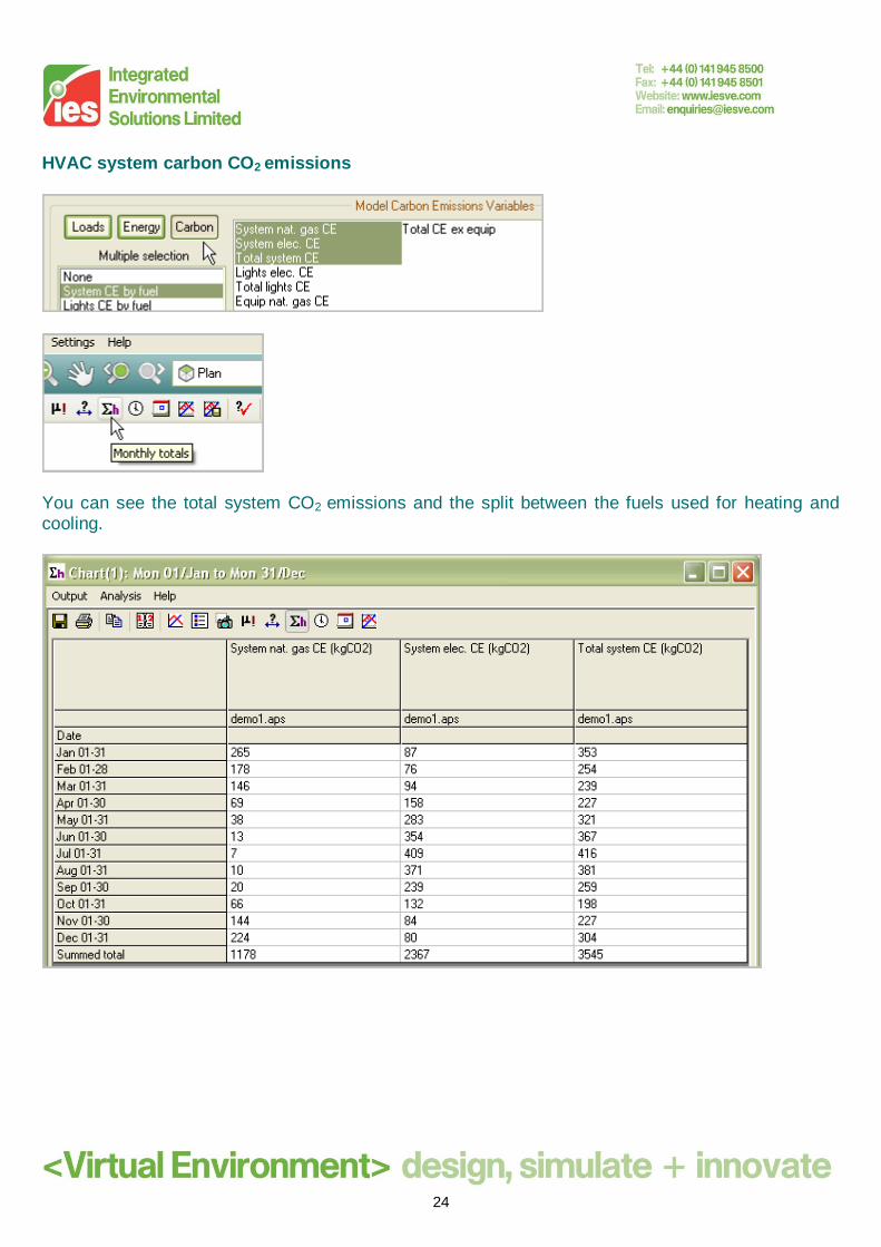
HVAC system carbon CO2 emissions

You can see the total system CO2 emissions and the split between the fuels used for heating and cooling.

25

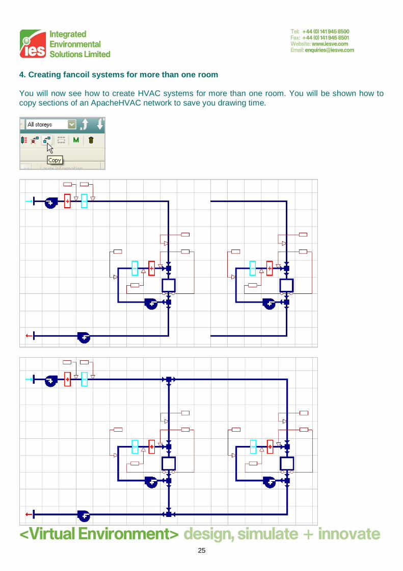
4. Creating fancoil systems for more than one room You will now see how to create HVAC systems for more than one room. You will be shown how to copy sections of an ApacheHVAC network to save you drawing time.

26

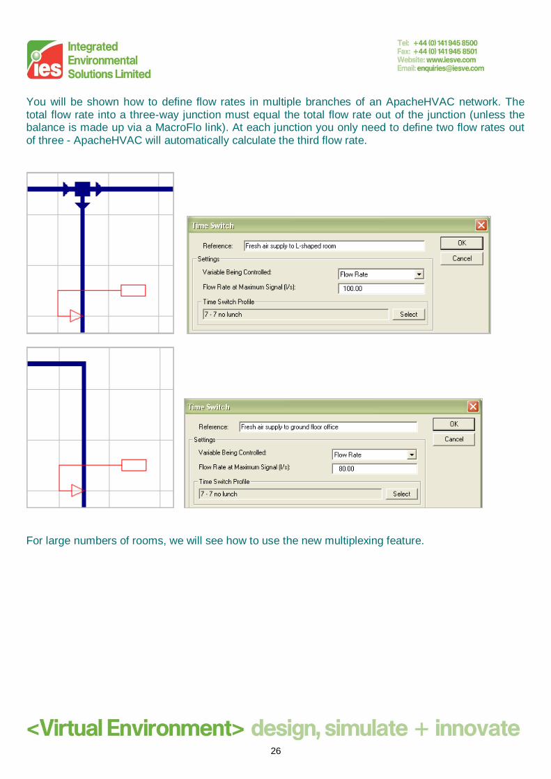
You will be shown how to define flow rates in multiple branches of an ApacheHVAC network. The total flow rate into a three-way junction must equal the total flow rate out of the junction (unless the balance is made up via a MacroFlo link). At each junction you only need to define two flow rates out of three - ApacheHVAC will automatically calculate the third flow rate.

For large numbers of rooms, we will see how to use the new multiplexing feature.

27

5. An introduction to Multiplexing You have been shown previously (when we created fancoil systems for more than one room) how to copy sections of a network and to connect the sections using junctions. With a large number of rooms however, the ApacheHVAC schematic view would become very cluttered and unwieldy. You will be shown how to use the new multiplexing feature which allows you to vertically “stack” similar rooms/systems and which allows you to make quick edits to one or more systems in the “stack”. You will see how to select items in the schematic you wish to multiplex.

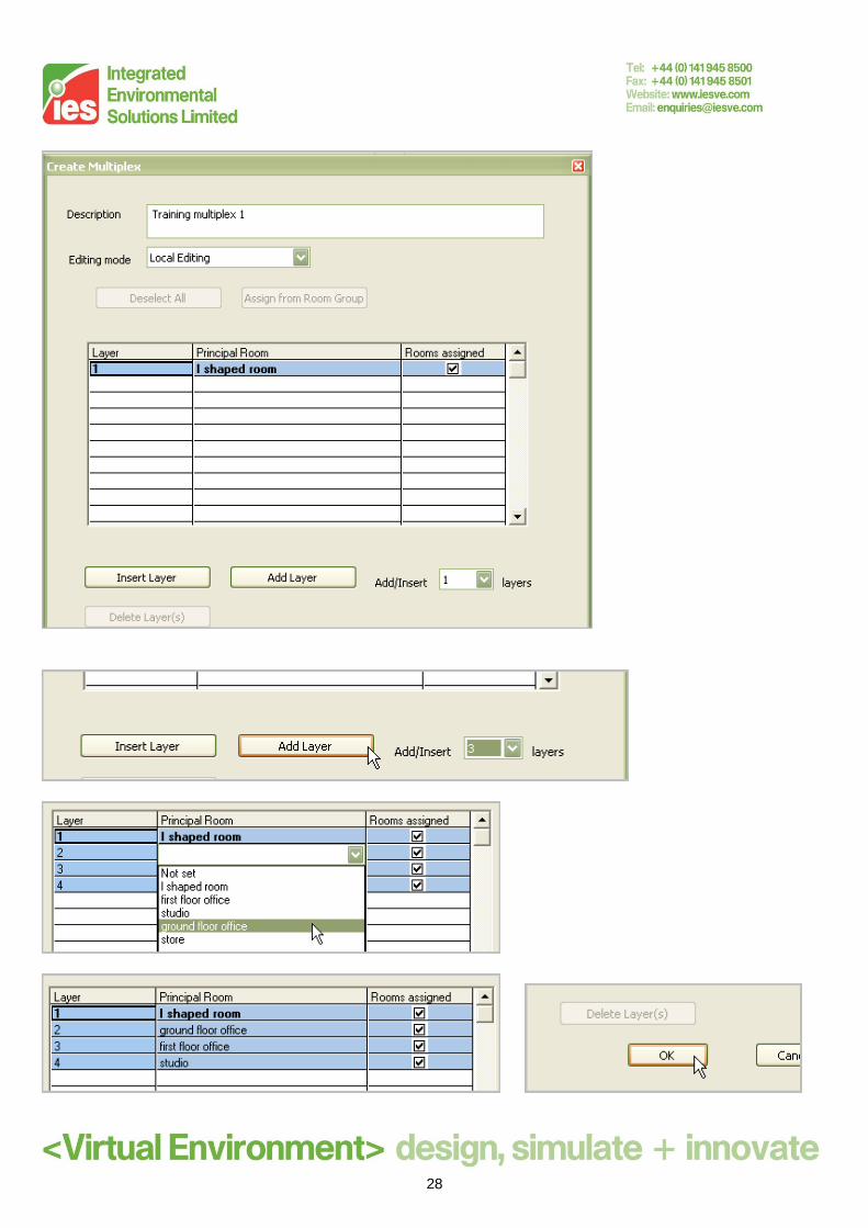
28

29

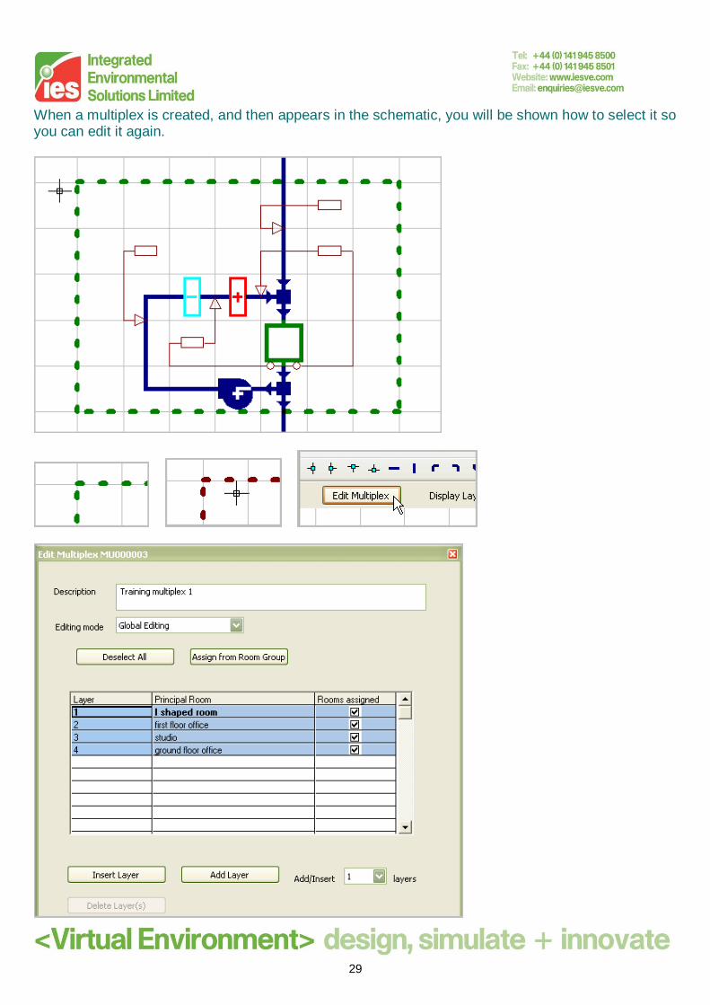
When a multiplex is created, and then appears in the schematic, you will be shown how to select it so you can edit it again.

30

Once you have created a multiplex, you can edit a variable of a component or control within the multiplex, for all the currently selected layers within the multiplex.

31

You can enter values individually for each layer in the table, or, for example, if you have coil size requirements or flow rates in a spreadsheet (or in Vista) after having performed load calculations, you can copy and paste a column of coil sizes or flow rates into the table.

32

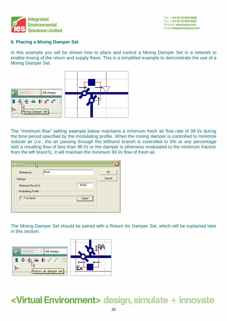
6. Placing a Mixing Damper Set In this example you will be shown how to place and control a Mixing Damper Set in a network to enable mixing of the return and supply flows. This is a simplified example to demonstrate the use of a Mixing Damper Set.

The “minimum flow” setting example below maintains a minimum fresh air flow rate of 99 l/s during the time period specified by the modulating profile. When the mixing damper is controlled to minimize outside air (i.e., the air passing through the lefthand branch is controlled to 0% or any percentage with a resulting flow of less than 99 l/s or the damper is otherwise modulated to the minimum fraction from the left branch), it will maintain the minimum 99 l/s flow of fresh air.

The Mixing Damper Set should be paired with a Return Air Damper Set, which will be explained later in this section.

33

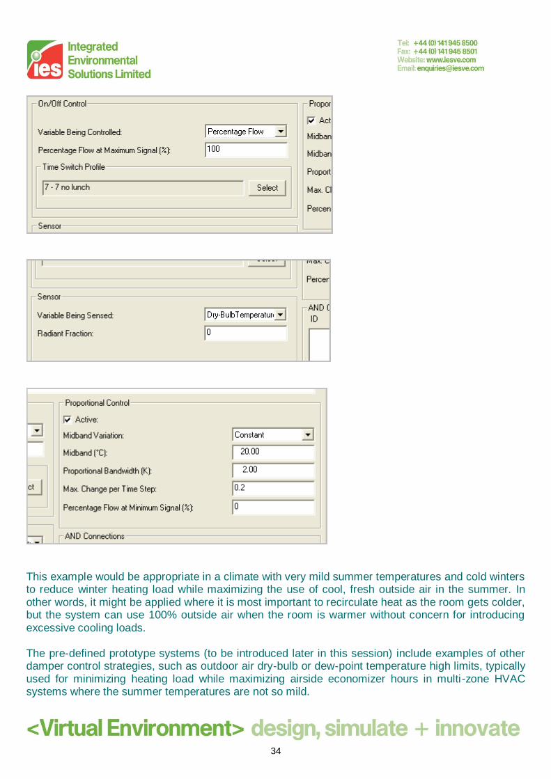
Controlling the Mixing Damper Set We will control the Mixing Damper Set using an Independent Controller with a Sensor. Using the settings below, the mixing damper will allow 100% of air through the lefthand (fresh air supply) branch when the room is warm and will recirculate all but the required 99 l/s minimum fresh air through the lower (return) branch when the room is cold.

34

This example would be appropriate in a climate with very mild summer temperatures and cold winters to reduce winter heating load while maximizing the use of cool, fresh outside air in the summer. In other words, it might be applied where it is most important to recirculate heat as the room gets colder, but the system can use 100% outside air when the room is warmer without concern for introducing excessive cooling loads. The pre-defined prototype systems (to be introduced later in this session) include examples of other damper control strategies, such as outdoor air dry-bulb or dew-point temperature high limits, typically used for minimizing heating load while maximizing airside economizer hours in multi-zone HVAC systems where the summer temperatures are not so mild.

35

Using the Return Air Damper Set

The Return Air (RA) Damper Set component is intended for use only with the Mixing Damper Set, and this is assumed to be when the Mixing Damper Set is functioning as an outside air (OA) economizer, i.e. when it is mixing OA and RA flows. The Return Air Damper Set has no separate user inputs and performs its function only when paired with the Mixing Damper Set. In order for the two to be linked, the RA Damper must be present on the vertical branch entering the Mixing Damper, and there can be no junctions between them. If it is not paired with the Mixing Damper in this configuration, it will revert to functioning as a simple junction. The linked RA Damper then acts to incrementally increase the minimum flow of outside air (makeup air) entering the system via the Mixing Damper when required. In other words, it can, as needed, override the minimum OA setting (the “minimum flow” setting) for the Mixing Damper.

The capability of the RA Damper link to automatically “override” the minimum OA setting in the Mixing Damper is useful in the case of any system for which the sum total of RA plus minimum OA available to the system may occasionally be less than the collective demand for primary airflow to the conditioned zones. This may occur, for example, when there are separately exhausted zones (e.g. lavatories, locker rooms etc) or variable-volume vent hoods (e.g., in laboratories, hospitals, etc.) actively removing air from the system according to schedules or sensed variables that are independent of the primary airflow controls to the conditioned zones that feed them (typically via transfer air).

36

7. Creating a system with heat recovery Here you will be shown how to place and control a heat recovery unit in a network.

37

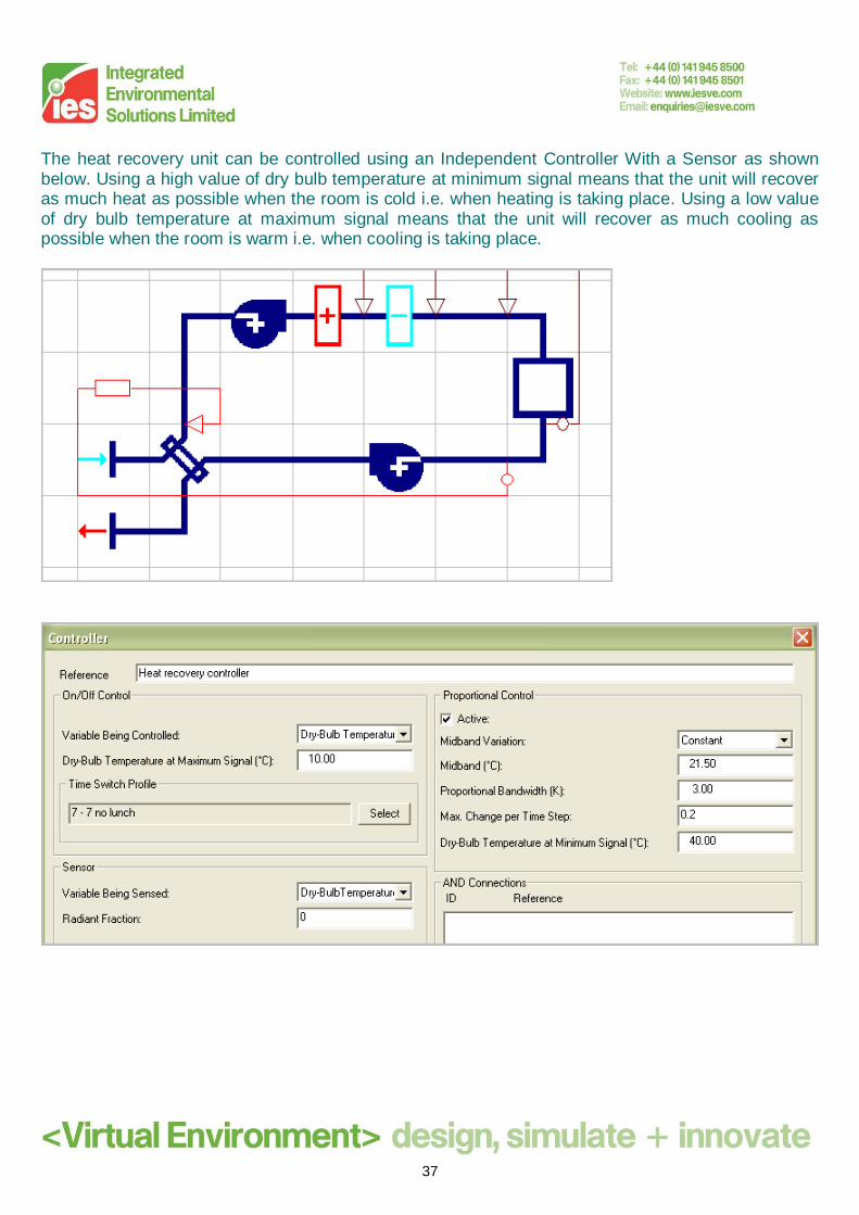
The heat recovery unit can be controlled using an Independent Controller With a Sensor as shown below. Using a high value of dry bulb temperature at minimum signal means that the unit will recover as much heat as possible when the room is cold i.e. when heating is taking place. Using a low value of dry bulb temperature at maximum signal means that the unit will recover as much cooling as possible when the room is warm i.e. when cooling is taking place.

38

8. Multiple controls for a component A new feature now allows you to control a component with more than one control. To be able to use multiple controllers for one component, both controls must be controlling the same variable, and both controls must be pointed to the same node. In the case of controllers with a sensor, the two controllers can be sensing different variables.

In this example, room humidity as well as room maximum temperature is controlled. There are two controls (each is an Independent Controller with a Sensor) controlling the cooling coil. The first control is used to control humidity and the second one is used to control the maximum temperature in the room.

39

In the first controller the off-coil temperature is varied according to the sensed room relative humidity.

The settings below mean that the cooling coil will operate as required to keep the room humidity in the band 37.5% to 42.5 %, subject to its capacity and other variables.

40

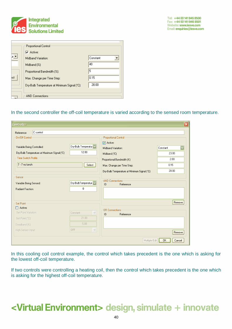
In the second controller the off-coil temperature is varied according to the sensed room temperature.

In this cooling coil control example, the control which takes precedent is the one which is asking for the lowest off-coil temperature. If two controls were controlling a heating coil, then the control which takes precedent is the one which is asking for the highest off-coil temperature.

41

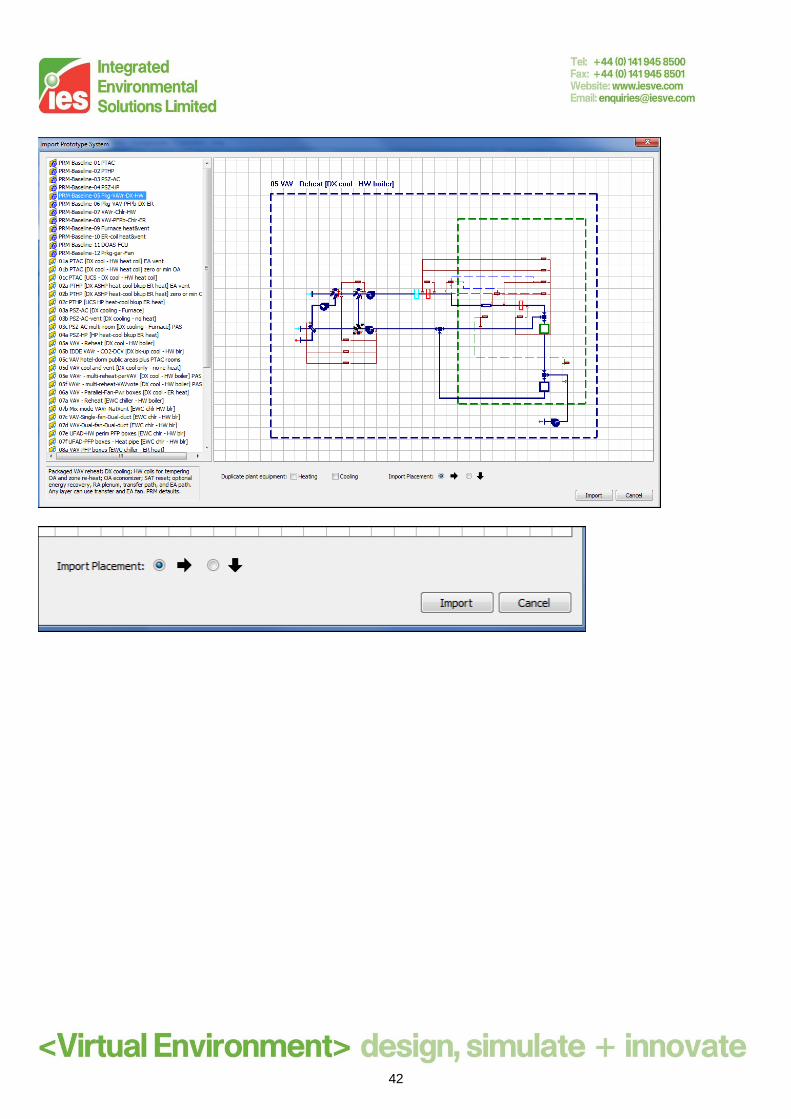
9. An introduction to the Prototype Systems library A recently added feature in ApacheHVAC is a library of ready-made, commonly used HVAC systems (prototype systems). You can select from this library and import one or more systems into your ApacheHVAC network. Once you have done this you can then edit these systems to suit your project.

42

43

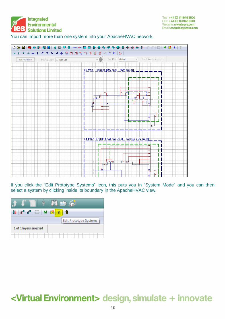
You can import more than one system into your ApacheHVAC network.

If you click the “Edit Prototype Systems” icon, this puts you in “System Mode” and you can then select a system by clicking inside its boundary in the ApacheHVAC view.

44

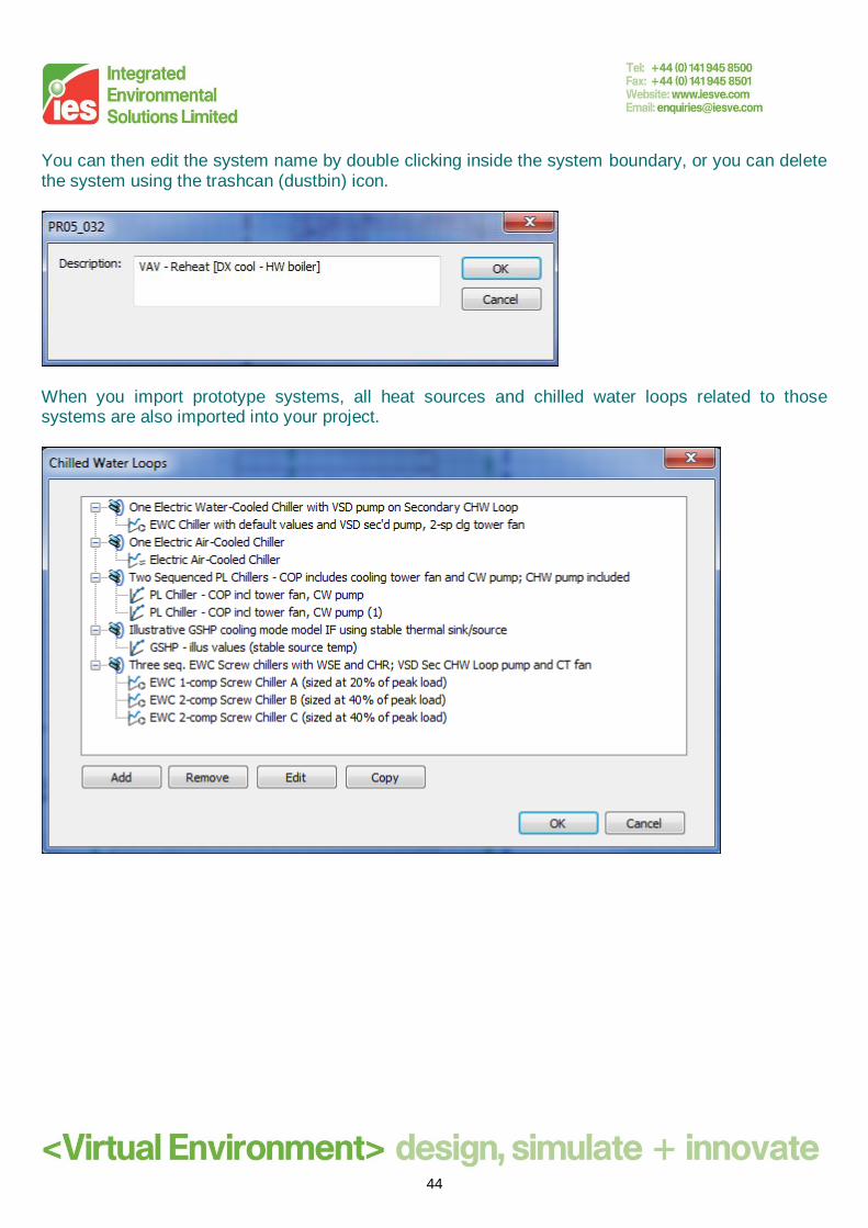
You can then edit the system name by double clicking inside the system boundary, or you can delete the system using the trashcan (dustbin) icon.

When you import prototype systems, all heat sources and chilled water loops related to those systems are also imported into your project.

45

10. An introduction to advanced chiller modelling In Session A you were shown how to create chillers by entering part load data. If required, you can enter data in more detail for electric water cooled (EWC chillers) or electric air cooled (EAC) chillers. In this section we will provide a brief introduction to advanced chiller modelling.

For an EWC or an EAC, the data in the Chilled Water Loop tab needs to be specified. Pump power and efficiency is entered for chilled water pumps, and the performance curve is selected for the secondary circuit.

46

For an EWC, the data in the Heat Rejection tab needs to be specified and the “Uses Condenser Water Loop?” option must be enabled. Cooling tower data (approach, range and fan data) is entered. Pump power is entered for condenser water pumps.

47

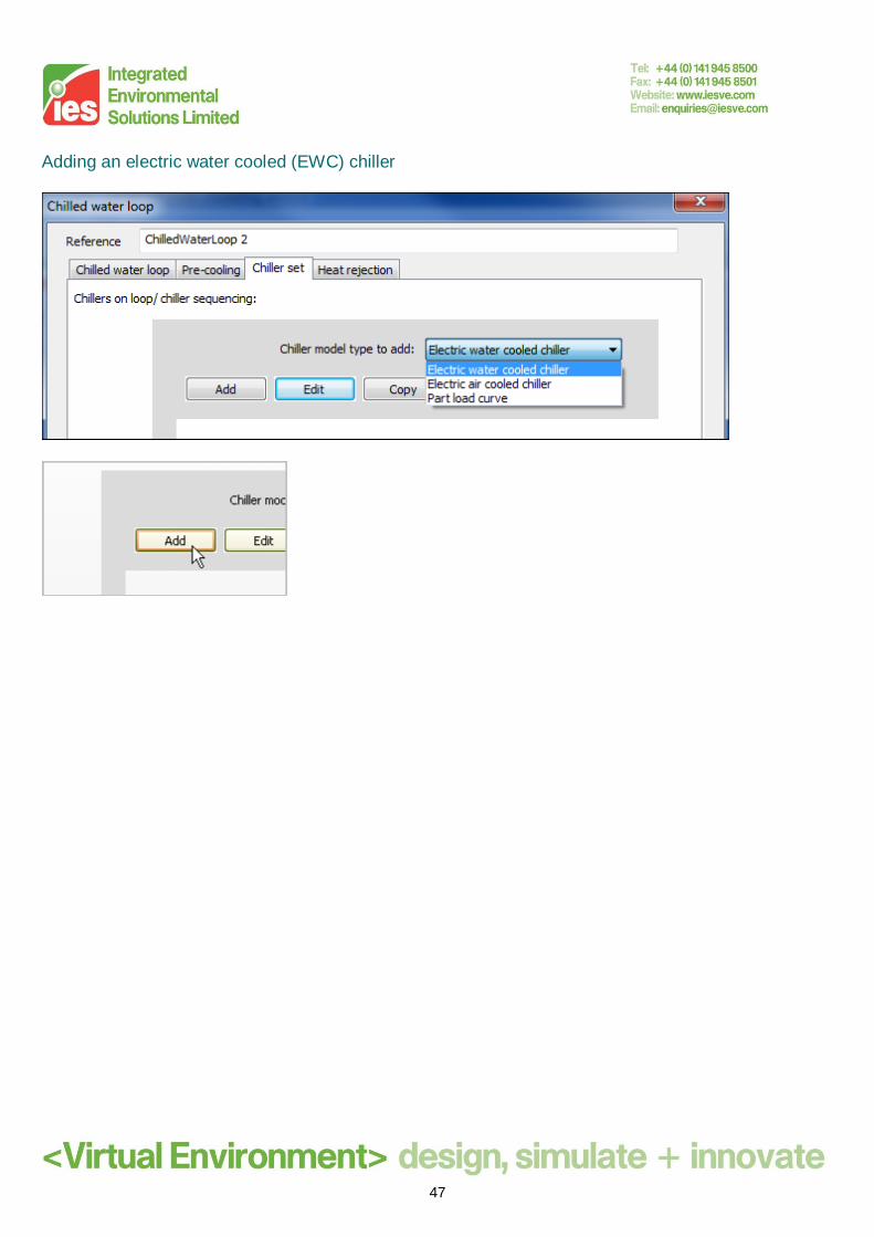
Adding an electric water cooled (EWC) chiller

48

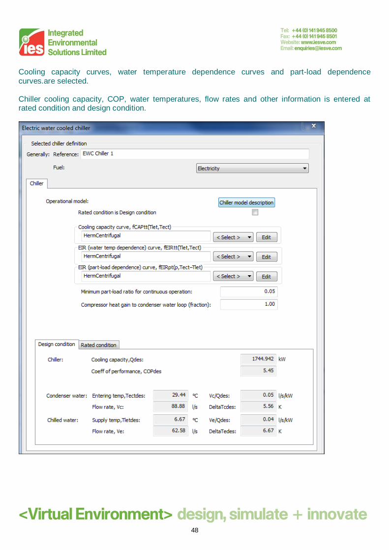
Cooling capacity curves, water temperature dependence curves and part-load dependence curves.are selected. Chiller cooling capacity, COP, water temperatures, flow rates and other information is entered at rated condition and design condition.

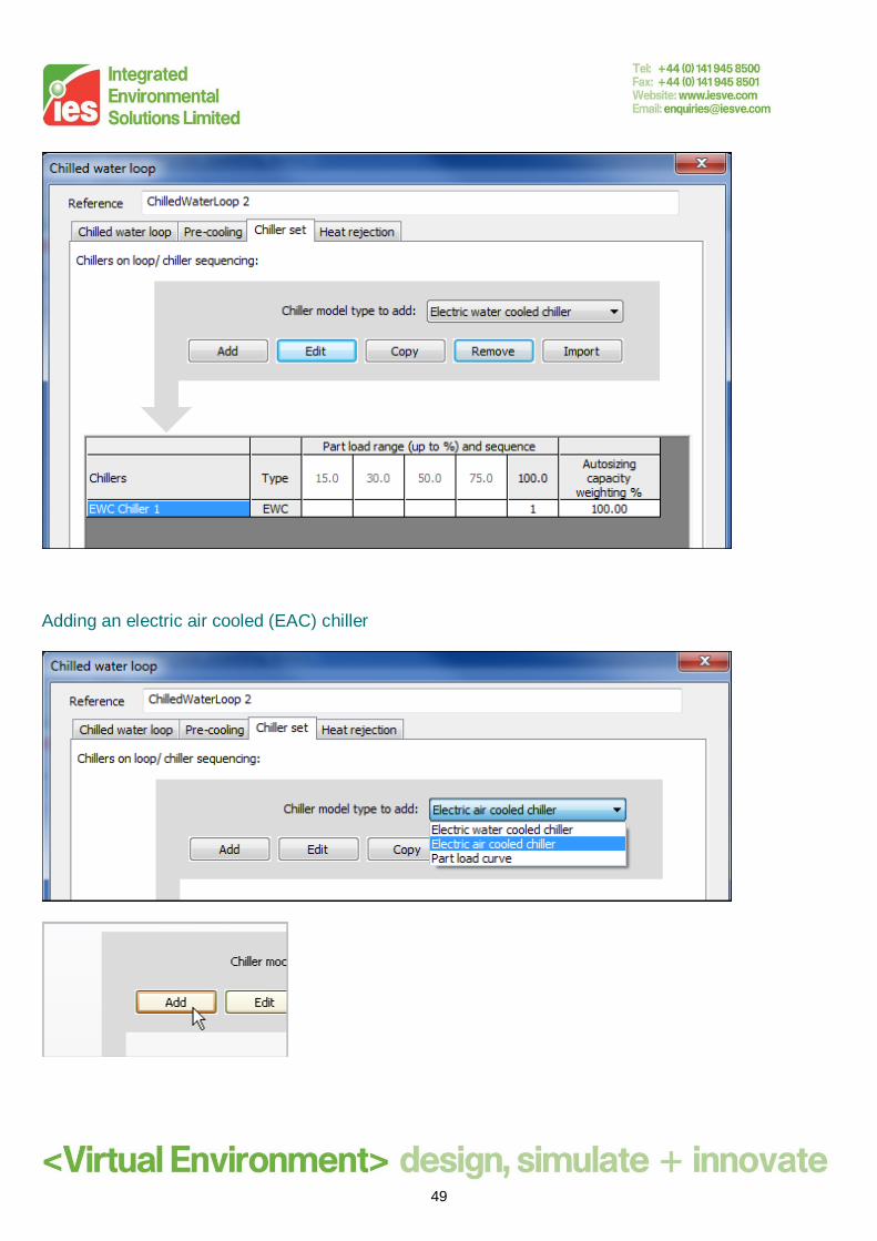
49

Adding an electric air cooled (EAC) chiller

50

51

We have now finished Session B.