ieee transactions on visualization and …cg.cs.tsinghua.edu.cn/people/~yongjin/fwp-tvcg.pdf ·...

IEEE TRANSACTIONS ON VISUALIZATION AND COMPUTER GRAPHICS, VOL. 21, NO. 7, PP. 822-834, 2015 1

Fast Wavefront Propagation (FWP) forComputing Exact Geodesic Distances on

MeshesChunxu Xu, Tuanfeng Y. Wang, Yong-Jin Liu, Member, IEEE,

Ligang Liu, Member, IEEE, and Ying He, Member, IEEE

Abstract—Computing geodesic distances on triangle meshes is a fundamental problem in computational geometry andcomputer graphics. To date, two notable classes of algorithms, the Mitchell-Mount-Papadimitriou (MMP) algorithm and theChen-Han (CH) algorithm, have been proposed. Although these algorithms can compute exact geodesic distances if numericalcomputation is exact, they are computationally expensive, which diminishes their usefulness for large-scale models and/or time-critical applications. In this paper, we propose the fast wavefront propagation (FWP) framework for improving the performanceof both the MMP and CH algorithms. Unlike the original algorithms that propagate only a single window (a data structure locallyencodes geodesic information) at each iteration, our method organizes windows with a bucket data structure so that it canprocess a large number of windows simultaneously without compromising wavefront quality. Thanks to its macro nature, theFWP method is less sensitive to mesh triangulation than the MMP and CH algorithms. We evaluate our FWP-based MMP andCH algorithms on a wide range of large-scale real-world models. Computational results show that our method can improve thespeed by a factor of 3-10.

Index Terms—Discrete geodesic, fast wavefront propagation, algorithm complexities

F

1 INTRODUCTION

HOW to compute shortest paths on polyhedralsurfaces is a fundamental problem in com-

putational geometry and computer graphics, whichhas been studied for almost three decades [1]. Todate, there are two notable classes of algorithms,namely, the Mitchell-Mount-Papadimitriou (MMP) al-gorithm [2] and the Chen-Han (CH) algorithm [3],which can compute exact geodesic distances on tri-angle meshes if numerical computation is exact. Al-though they are based on different domain subdivi-sion strategies, these two algorithms adopt a similardata structure called window, which locally encodesthe geodesic information.

It is known that both the MMP and CH algorithmsproduce O(n2) windows on an n-face triangle meshand the upper bound is tight [4]. Therefore, anywindow-based discrete geodesic algorithm cannot runfaster than O(n2) theoretically, which is known asthe quadratic time barrier. Interestingly, as shownin this paper, the correctness of the MMP and CHalgorithm is independent of the order of the windowsbeing processed. However, propagating windows in

• C. Xu and Y-J. Liu are with the TNList, Department of ComputerScience and Technology, Tsinghua University, China.

• T. Wang and L. Liu are with School of Mathematical Sciences,University of Science and Technology of China.

• Y. He is with School of Computer Engineering, Nanyang TechnologicalUniversity, Singapore.Corresponding authors: Yong-Jin Liu & Ying He

an arbitrary order results in an extremely poor per-formance. The MMP algorithm keeps windows ina priority queue, where the window closest to thesource is taken at each iteration. Since each windowoperation (i.e., choosing a window from the priorityqueue and propagating it) takes O(log n) time, theMMP algorithm has an O(n2 log n) time complexity.The CH algorithm, in contrast, maintains windowsin a hierarchical structure and processes them in abreadth-first-search order, resulting in an O(n2) timecomplexity. However, computational results in [5] [6]show that the MMP algorithm runs much faster thanthe CH algorithm.

Xin and Wang [7] observed that the slow perfor-mance of the CH algorithm is mainly due to the largeamount of useless windows processed. They proposeda simple yet effective window filter to detect theuseless windows, accompanied by a priority queue forwindow organization. The improved CH algorithm,called ICH, has a speed comparable to the MMPalgorithm, however, its theoretical time complexitybecomes O(n2 log n) due to the priority queue. Todate, developing an O(n2) exact discrete geodesicalgorithm with good practical performance is still agreat challenge.

This paper tackles this challenge by proposing afast wavefront propagation (FWP) framework, whichbridges the gap between theoretical time complexityand practical performance of discrete geodesic algo-rithms. Unlike the MMP and ICH algorithms thatpropagate only a single window (the one closest to


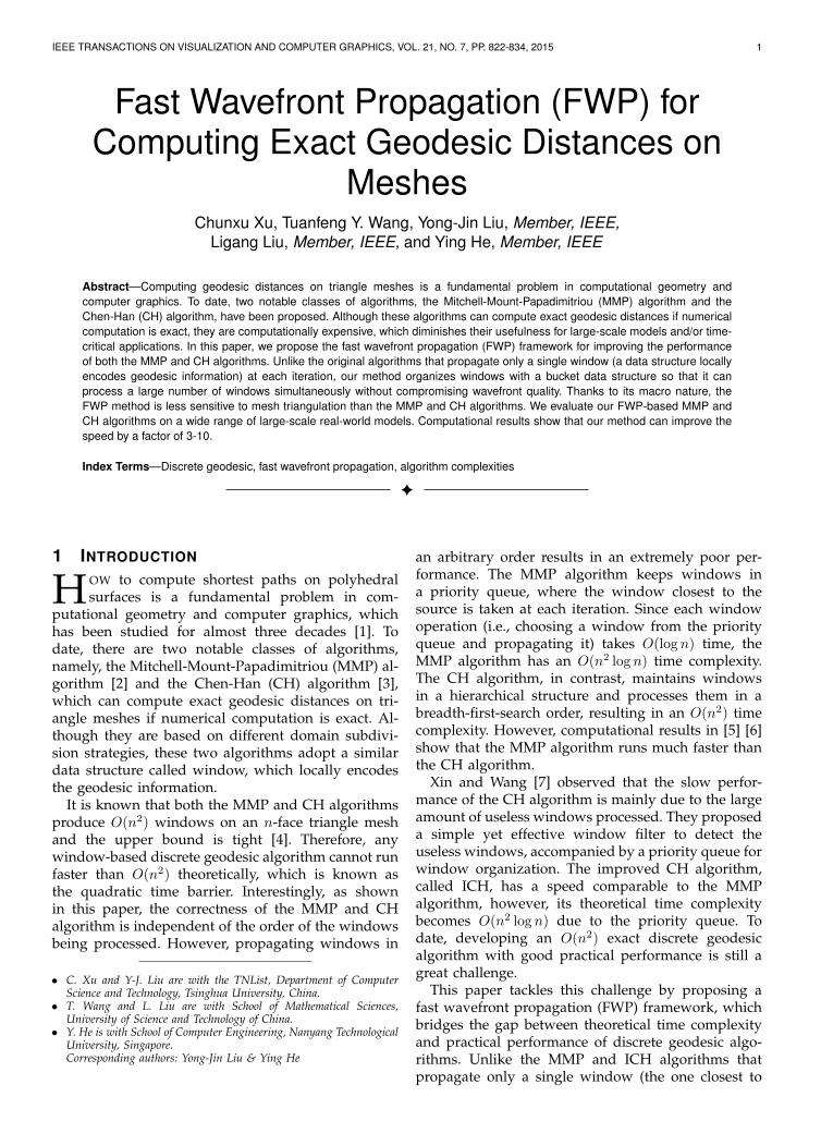
MMP: 89, 047, 334 iterations, 320.6s Dragon: 4M faces FWP-MMP: 13, 748 iterations, 31.7s

Fig. 1. Choose the source vertex at the nose of the 4M-face Dragon model. The existing undiscretized geodesic algorithms(e.g., MMP and ICH) have poor performance since they propagate the wavefronts very slowly. Our fast wavefront propagationtechnique can significantly improve their speed. Each colored curve is a discrete wavefront and the 2-tuple associated witheach wavefront is the iteration number and the corresponding time, which was measured on a PC with an Intel Core i7-2600CPU (3.40 GHz). We draw only a few representative wavefronts to avoid clutter. The small inset in the middle illustrates thecomputed geodesic distances using iso-distance contours.

the source) at each iteration, our method organizeswindows in a bucket data structure so that it is ableto process a large number of windows simultaneouslywithout compromising wavefront quality. Althougha window may enter and leave the bucket multi-ple times, our method guarantees that the windowcomplexity is still O(n2). Since the practical overheadrequired for each iteration is very small, our FWP-based MMP and CH algorithms run faster than theoriginal algorithms. Computational results on real-world models show that our method improves theperformance by a factor of 3-10. See Figure 1 foran example. Intuitively speaking, the performanceimprovement by our method is due to its efficientdata organization on a macro scale (i.e., focusing onwavefronts consisting of many windows), whereas theexisting algorithms are on a micro scale (i.e., focusingon an individual window). Thanks to its macro na-ture, the FWP-based methods are also less sensitiveto mesh resolution than the MMP and CH algorithms,i.e., increasing the mesh anisotropy may significantlyslow down the existing algorithms, but it affects theFWP-based methods slightly.

In this paper our contributions are twofold:First, from a theoretical perspective, the FWP frame-

work unifies the two classes of algorithms from themacro scale: the FWP-CH and FWP-MMP algorithmspropagate the wavefronts at a similar pace and theyconverge in roughly the same number of iterations,although their window propagation schemes are verydifferent. The FWP framework has provable time andspace complexity: the FWP-CH and FWP-MMP algo-rithms have O(n2) and O(n2 log n) time complexity,respectively.

Second, from a practical perspective, the FWP tech-nique is easy to implement and it can speedup the

MMP and CH algorithms significantly. It is worthnoting that the FWP-MMP algorithm can improve theperformance of the MMP algorithm by an order ofmagnitude on large-scale real-world models, makingit comparable to the state-of-the-art GPU-based par-allel Chen-Han algorithm [8]. As a macro algorithm,the FWP-CH and FWP-MMP algorithms are also lesssensitive to mesh triangulation than the existing microalgorithms. We also demonstrate that the FWP-basedalgorithm can be applied to the pre-computationmethods, such as Saddle Vertex Graph (SVG) [9] andGeodesic Triangle Unfolding (GTU) [10].

2 RELATED WORK

Classic techniques for computing discrete geodesicson triangle meshes include the computational geome-try approaches and the partial differential equation(PDE) approaches. The former includes the above-mentioned MMP/CH algorithms and their many vari-ants [5] [6] [7] [8] [11] [12]. The latter consists of thepopular fast marching method (FMM) [13], [14] andthe gradient-based approaches [15][16]. See [1] for acomprehensive survey of classic techniques.

Each type of technique has its own merits and limi-tations. The undiscretized methods such as MMP andCH in computational geometry approaches can obtainthe exact geodesics on arbitrary triangle meshes ifnumerical operations are exact. As a comparison, thePDE approaches provide only the approximate solu-tions (e.g., the first-order approximation by the FMM),which may be poor on meshes with highly irregulartessellation. On the other hand, the PDE approachesare usually faster than the computational geometryapproaches. But they assume that the triangle meshesare discrete samples of underlying smooth surfacesand proving the convergence of the discrete geodesic


S

p

1w

1w2w

3w

(a) Covered regions of windows

e0v

1vA B

2v

0d

1d

2d

p

x

y

S

10

(b) 2D parameterization

Fig. 2. (a) A window w is an interval (drawn in red) on amesh edge such that the geodesic paths from the source toany point inw have the same face sequence (colored in pink).Propagating a window across an edge produces one or morechild windows. w1 has one child and w2 has two children.Both w1 and w2 are directly visible from the source s, but w3

is not. Instead, w3 is visible from the pseudo source p. (b)Parameterizing a window to R2 locally encodes the geodesicdistance from the source s to any point on the window.

distance to its smooth counterpart is of important the-oretical value; e.g., uniform convergence of geodesicsis proved in [17] under the assumption of convergenceof surfaces in Hausdorff distance.

Recently precomputation techniques have been pro-posed, which aim at balancing quality and per-formance for computing various types of discretegeodesics. Xin et al. [10] proposed the Geodesic Tri-angle Unfolding (GTU) method, which flattens thecurved geodesic triangle onto R2 and then uses Eu-clidean distance to approximate geodesic distance.The heat method, proposed by Crane et al. [16], isan elegant gradient based approach, which recoversthe geodesic distance from the normalized gradient ofthe heat flow. By pre-factoring the Laplacian matrix,both the heat flow and the distance computation canbe done in near-linear time. The heat method is easyto implement. It is also flexible to support a widerange of geometric domains, including grids, trianglemeshes and point clouds. Such a feature is not avail-able in the computational geometry approaches thatwork only for triangle meshes. However, similar tothe FMM, it provides only a first order approximation.

Observing that the discrete geodesic problem hasa surprisingly strong local structure due to the ex-istence of the saddle vertices, Ying et al. [9] pro-posed another precomputation technique called thesaddle vertex graph (SVG), a sparse graph whichencodes the geodesic information on triangle meshes.With the SVG, computing the polyhedral distance isequivalent to finding the shortest path on the graph.Note that the pre-computation of both the GTU andSVG methods heavily depends on the MMP or ICHalgorithm. As the proposed FWP technique improvestheir performance significantly, we show that it canbe adopted in the GTU and SVG methods to reducetheir precomputation time.

3 PRELIMINARYLet M = (V,E, F ) be a triangle mesh, where V , E andF are the sets of vertices, edges and faces, respectively.Given a source point s ∈ V , Mitchell et al. [2] showedthat a geodesic path from s to vertex vj passes througha sequence of mesh faces. A window is an intervalI defined on a mesh edge such that the geodesicpaths from s to any point in I share the same facesequence. See Figure 2(a). Mitchell et al. also showedthat a geodesic path cannot pass through any spheri-cal vertex (a vertex at which the sum of surroundingangles is less than 2π) unless it is the destination,since perturbing the path a bit off the spherical vertexreduces its length. However, a geodesic path may passthrough one or more saddle vertices (a vertex at whichthe sum of surrounding angles is greater than 2π).The saddle vertex nearest to the destination is calleda pseudo source. A window associated with a half-edgee is a 6-tuple (σ,A,B, σ0, σ1, e) [5] where• σ is the distance from the pseudo source p to the

source s;• A and B are the left and right endpoints of the

interval;• σ0 and σ1 are the distances from I’s endpoints top.

With this window data structure, we can easily po-sition the source or pseudo source in the unfoldedface/edge sequences and compute the geodesic dis-tance for any point inside the interval. See Figure 2(b).Note that the MMP algorithm stores oriented win-dows so that each side of a non-boundary edge con-tains windows, whereas the CH algorithm does notrequire edge orientation.

The MMP and CH algorithms maintain a vector(d1, · · · , dn), n = |V |, for the polyhedral distancesdefined on mesh vertices, and a set of windows W .Initially, we have ds = 0 and di = ∞ for i 6= s. SetW contains the windows covering the edges oppositeto the source vertex s. The algorithms then iterativelypropagate windows across the faces and update thepolyhedral distances when a window covers a vertexor part of an edge, until the set W is empty. Upontermination, label di is the geodesic distance from thesource s to vertex vi. The computational frameworkof the MMP and CH algorithms is as follows:

while W is not empty doextract a window w = (σ,A,B, σ0, σ1, e) from W ;if e is not a boundary edge then

propagate w across e to produce child windows w;update the distance of vertex/edge covered by w;add w to W ;

end ifend while

Both the MMP and CH algorithms have O(n2)window complexity. They are distinguished by thedata structure for organizing the windows and theorder of window processing. The MMP algorithmmaintains a priority queue for the windows and takes


the window closest to the source in each iteration. Asa result, the MMP algorithm has an O(n2 log n) timecomplexity. The CH algorithm records the parent-child relationship of windows in a hierarchical treestructure and processes the windows in a breadth-first-search order, which is implemented by a first-in-first-out (FIFO) queue. Therefore, the CH algorithmhas an O(n2) time complexity. The ICH algorithmadopts a simple-yet-effective window filter, whichcan reduce many useless windows. Furthermore, ituses the priority queue to organize the windowsaccording to their distance back to the source. TheICH algorithm, with a time complexity O(n2 log n),significantly outperforms the CH algorithm in termsof speed.

4 FAST WAVEFRONT PROPAGATION

A wavefront in a continuous setting is the locus ofpoints having the same distance to the source. TheMMP/CH/ICH algorithms maintain a discrete wave-front, which can be formally defined as follows:

Definition 1. The i-th wavefront, denoted by Wi, is theunion of windows in W at the i-th iteration.

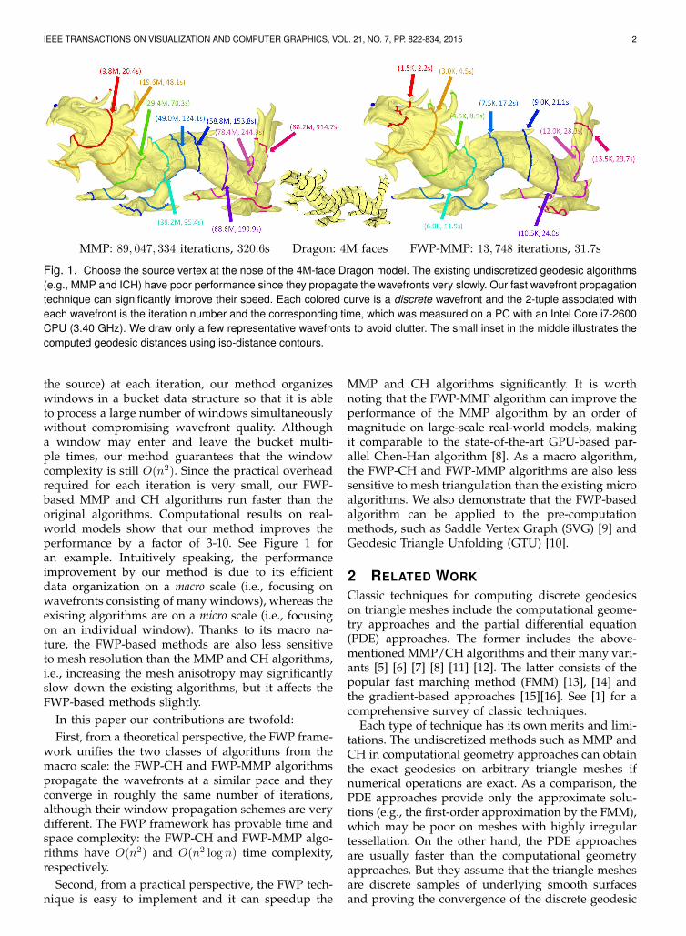
A wavefront depends on the model, the location ofthe source point, as well asthe time, and it may be un-connected. As the right insetshows, each color correspondsto one wavefront. At the be-ginning, the wavefront is con-nected and has a circular shape.Later, it evolves to several con-nected components. Finally, eachconnected component shrinks toa maximal point (where thegeodesic distance reaches the lo-cal maximum) and then van-ishes. For a window w, we define its label as theshortest distance from the source to w’s associatedmesh edge. The size of Wi, denoted by |Wi|, is de-termined by the number of windows it has. The stan-dard deviation of all window labels in Wi, std(Wi),is a good measure of wavefront quality. Intuitivelyspeaking, the smaller the variance, the higher qualitythe wavefront has. Wavefront quality depends on theorder of windows being processed. As shown in Fig-ure 3, propagating windows in the smallest-label-firstorder leads to a high-quality wavefront (i.e., smoothand with small variance), whereas using the first-in-first-out order produces a low-quality wavefront (i.e.,very rough and with large variance).

The MMP and ICH algorithms always take thewindow with the minimal label at each iteration,resulting in a high-quality wavefront. However, theoverhead required for each iteration is expensive.Computational results show that more than 60% of the

(a) Priority queue-based wavefront

(b) FIFO queue-based wavefront

Fig. 3. The MMP algorithm maintains a priority queue for thewindows, leading to a high-quality wavefront with standarddeviation std = 0.00219. Replacing the priority queue by anFIFO queue results in a very poor and slow-moving wavefrontwith std = 0.02431. The model has been scaled to a unitcube.

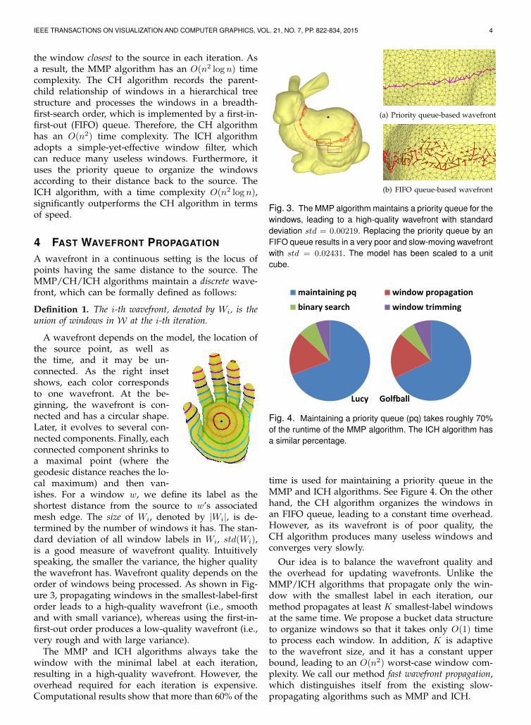
maintaining pq window propagation

binary search window trimming

Lucy Golfball

Fig. 4. Maintaining a priority queue (pq) takes roughly 70%of the runtime of the MMP algorithm. The ICH algorithm hasa similar percentage.

time is used for maintaining a priority queue in theMMP and ICH algorithms. See Figure 4. On the otherhand, the CH algorithm organizes the windows inan FIFO queue, leading to a constant time overhead.However, as its wavefront is of poor quality, theCH algorithm produces many useless windows andconverges very slowly.

Our idea is to balance the wavefront quality andthe overhead for updating wavefronts. Unlike theMMP/ICH algorithms that propagate only the win-dow with the smallest label in each iteration, ourmethod propagates at least K smallest-label windowsat the same time. We propose a bucket data structureto organize windows so that it takes only O(1) timeto process each window. In addition, K is adaptiveto the wavefront size, and it has a constant upperbound, leading to an O(n2) worst-case window com-plexity. We call our method fast wavefront propagation,which distinguishes itself from the existing slow-propagating algorithms such as MMP and ICH.


Ki+1 = Ki + (clarge – csmall) = 12;

(a) Initialization

Buckets

(b) At the beginning of the current iteration

Buckets

(d) An intermediate step of the current iteration

Buckets

(e) The current iteration ends

Buckets

windows born in early iterations

windows born in the current iteration

propagation

1 2/P P endP16;iK

1P2P endP

6; 11;large smallc c

1P 2 / endP P13; 17;large smallc c

(c) The current iteration starts

Buckets

1 2/P P endP0; 2;large smallc c

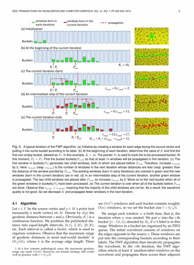
Fig. 5. A typical iteration of the FWP algorithm. (a) Initialize by creating a window for each edge facing the source vertex andputting it into some bucket according to its label. (b) At the beginning of each iteration, determine the value of K and find thefirst non-empty bucket, labeled as P1. In this example, K = 16. The pointer P2 is used to track the to-be-processed bucket. Atthis moment, P2 = P1. Find the bucket buckets[Pend] so that at least 16 windows will be propagated in this iteration. (c) Thefirst window in buckets[P2] generates two child windows, both of which are placed before Pend. Therefore, increase csmall

by 2. Here csmall (resp. clarge) is the number of windows in the next iteration whose distances are less (resp. greater) thanthe distance of the window pointed by Pend. The existing windows (born in early iterations) are colored in green and the newwindows (born in the current iteration) are in red. (d) In an intermediate step of the current iteration, another green windowis propagated. The two child windows are placed after Pend, so increase clarge by 2. Move on to the next bucket when all ofthe green windows in buckets[P2] have been processed. (e) The current iteration is over when all of the buckets before Pend

are done. Observe that clarge < csmall, meaning that the majority of the child windows are not far. As a result, the wavefrontquality is not good. So we decrease K and propagate fewer windows in the next iteration.

4.1 AlgorithmLet s ∈ V be the source vertex and p ∈M a point (notnecessarily a mesh vertex) on M . Denote by d(p) thegeodesic distance between s and p. Obviously, d(·) is acontinuous function. We partition the polyhedral dis-tance into equal-length intervals, [0, l), [l, 2l), [2l, 3l),etc. Each interval is called a bucket, which is used toorganize windows. Observe that the maximum rangeof geodesic distances in most real-world models1 isO(√nh), where h is the average edge length. There

1. In a few extreme pathological cases, the maximum geodesicrange can reach O(nh). However, our bucket strategy still workswell in practice with l = h/

√n.

are O(n2) windows and each bucket contains roughlyO(n) windows, so we set the bucket size l = h/

√n.

We assign each window w a birth time, that is, theiteration when w was created. We put w into the i-thbucket [(i−1)l, il), denoted by Bi, if w’s label is in thisrange. Windows in a bucket are organized by an FIFOqueue. The initial wavefront consists of windows onthe edges opposite to the source s. These windows areput into the corresponding buckets according to theirlabels. The FWP algorithm then iteratively propagatesthe wavefront. In the i-th iteration, the FWP algo-rithm selects at least K smallest-label windows on thewavefront and propagates them across their adjacent


triangles. The number K is adapted to the size andquality of the wavefront, and K can be determinedautomatically. See Section 4.2.

Three pointers P1, P2 and Pend are used. The pointerP1 points to the first non-empty bucket and thepointer P2 is used to track the to-be-processed bucket.For each window w in buckets[P2] who were born insome iteration earlier than i, we propagate w acrossits adjacent triangle, and obtain one or more childwindows. Since a child window always has a largerdistance than its parent, it cannot be placed in a bucketbefore its parent. Note that some new windows (whoare born in the current iteration) may be added tothe bottom of the queue in buckets[P2]. If so, we skipthese windows (colored in red in Figure 5), and moveP2 to the next non-empty bucket.

The current iteration is over when it processes atleast K smallest-label windows who were born early(i.e., reaching the bucket pointed to by Pend that isdetermined at the beginning of current iteration). TheFWP algorithm terminates when all of the buckets areempty. Figure 5 illustrates a typical iteration of theFWP algorithm. See Algorithm 1 for the pseudocode.

The proposed FWP algorithm is a general frame-work for organizing and propagating windows sothat it can be applied to both the MMP and ICHalgorithms. In the following, we refer to the FWP-based MMP and ICH algorithms as FWP-MMP andFWP-CH, respectively.

4.2 Adaptive Adjustment of K

Setting K = 1 is too conservative, since only windowsin the first non-empty bucket propagate in each iter-ation and the overhead required for each iteration isexpensive, akin to the MMP/ICH algorithms. On theother hand, an extremely large K means that all thewindows on the wavefront are propagated at once,that is, without taking their distances into account.As a result, the wavefronts are of low quality and theFWP algorithm becomes the highly inefficient FIFO-based algorithm. Thus, an extremely large K is tooaggressive. We do expect a proper K for both high-speed wavefront propagation and the wavefronts ofhigh quality. Since the time-dependent wavefrontsmay change dramatically throughout the iterativeprocedure, the K value should be adaptive to thewavefront’s size and quality, and are updated at eachiteration.

Consider the i-th wavefront Wi. Denote by Ki thewindows propagated in i-th iteration. Since Ki isthe number of windows in buckets whose pointersrange from P1 to Pend, Ki is always equal to orlarger than K. Let τ denote the Ki-th smallest labelof the windows in Wi. Then we partition Wi intotwo sets, W 1

i and W 2i , where W 1

i consists of thewindows with distances less than τ and W 2

i = Wi\W 1i

contains the remaining windows. Note that the FWP

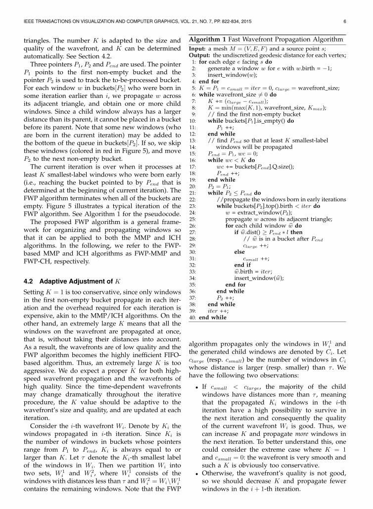
Algorithm 1 Fast Wavefront Propagation AlgorithmInput: a mesh M = (V,E, F ) and a source point s;Output: the undiscretized geodesic distance for each vertex;

1: for each edge e facing s do2: generate a window w for e with w.birth = −1;3: insert window(w);4: end for5: K = P1 = csmall = iter = 0, clarge = wavefront size;6: while wavefront size 6= 0 do7: K += (clarge − csmall);8: K = min(max(K, 1), wavefront size, Kmax);9: // find the first non-empty bucket

10: while buckets[P1].is empty() do11: P1 ++;12: end while13: // find Pend so that at least K smallest-label14: windows will be propagated15: Pend = P1, wc = 0;16: while wc < K do17: wc += buckets[Pend].Q.size();18: Pend ++;19: end while20: P2 = P1;21: while P2 ≤ Pend do22: //propagate the windows born in early iterations23: while buckets[P2].top().birth < iter do24: w = extract window(P2);25: propagate w across its adjacent triangle;26: for each child window w do27: if w.dist() ≥ Pend ∗ l then28: // w is in a bucket after Pend

29: clarge ++;30: else31: csmall ++;32: end if33: w.birth = iter;34: insert window(w);35: end for36: end while37: P2 ++;38: end while39: iter ++;40: end while

algorithm propagates only the windows in W 1i and

the generated child windows are denoted by Ci. Letclarge (resp. csmall) be the number of windows in Ci

whose distance is larger (resp. smaller) than τ . Wehave the following two observations:

• If csmall < clarge, the majority of the childwindows have distances more than τ , meaningthat the propagated Ki windows in the i-thiteration have a high possibility to survive inthe next iteration and consequently the qualityof the current wavefront Wi is good. Thus, wecan increase K and propagate more windows inthe next iteration. To better understand this, onecould consider the extreme case where K = 1and csmall = 0: the wavefront is very smooth andsuch a K is obviously too conservative.

• Otherwise, the wavefront’s quality is not good,so we should decrease K and propagate fewerwindows in the i+ 1-th iteration.


Inspired by these observations, we adaptively ad-just K by setting Ki+1 = Ki + (clarge − csmall). Thissimple strategy works remarkably well in practice. SeeSection 6 for detailed discussions.

4.3 Correctness & Complexity

The correctness of the FWP method relies on thefollowing proposition.

Proposition 1. Both the MMP and CH algorithms gen-erate correct solutions regardless of the order in which thewindows are processed in the queue.

Proof. First, note that (1) the useless windows willbe deleted when they are covered by other windowsarrived later that provide shorter distances to thesource and (2) for any windows that provide shortestdistances to the source, their parent windows alsoprovide shortest distances to the source. So all thewindows in the correct solution will appear in thequeue regardless of the window propagation order.

Second, we show that the algorithm will terminatein a finite number of steps regardless of the windowpropagation order. We assign an integer-valued levelto each candidate window (including both useful anduseless windows) in the queue. The windows facingthe source are at level 1. When a level-i windowis propagated, its child windows have level i + 1.Note that on an n-face mesh, a window’s level cannotexceed n. Assume that an algorithm randomly picksa window w and propagates it. Since the level of wand all its descendants should be not larger than n,w has a finite number of descendants. Thus the totalnumber of windows generated by this algorithm isfinite.

Note that Surazhsky et al. mentioned the aboveproperty (c.f. Section 3.4 [5]) but did not give a proof.

Our FWP method works well for real-world meshmodels, as indicated in the following property with amoderate realistic assumption.

Proposition 2. Assume that the degree of each vertex inM is bounded by a constant D. Both the FWP-MMP andFWP-CH algorithms produce O(n2) windows, and theyhave O(n2 log n) and O(n2) time complexity, respectively,where n is the number of vertices in M .

Proof. Upon the termination of the MMP or CH al-gorithm to the mesh M , we obtain a set of windowsstored in each edge and vertex. We call these windowsfinal, since they encode the shortest geodesic distance.In contrast, the windows, which were created duringwindow propagation and deleted later, are uselesswindows and not final.

In our FWP-based algorithm, Ki(≥ 1) windows ofsmallest labels are propagated at the i-th iteration.First note that the window of smallest label mustbe final since no other windows in the queue canreplace it later. Then in the propagated Ki windows,

they contain at least one final window. As long as awindow becomes final, its status remains unchangedthroughout the remaining iterations. Second, both theMMP and CH algorithms have no more than O(n2)final windows. Since at least one final window isextracted from the wavefront in each iteration, theFWP-based algorithm converges in O(n2) iterationsat most.

Note also that Ki is bounded by a constant Kmax

(Line 8 in Algorithm 1). Therefore, at most mKmax

child windows are generated and inserted into thebuckets, where m is the maximum number of childrena parent window can have. Thus, we have m ≤ D dueto the assumption that the degree is no more than D.Finally, the total number of windows inserted into thebuckets are O(DKmaxn

2) = O(n2).The FWP-MMP algorithm has an O(log n) overhead

at each iteration, since there are, at most, O(n) win-dows at each edge, and these windows are sortedin the same manner as the original MMP algo-rithm. Therefore, the FWP-MMP algorithm has anO(n2 log n) time complexity. For the FWP-CH algo-rithm, the overhead per iteration is O(1), resulting inan O(n2) time complexity.

5 EXPERIMENTAL RESULTSBoth the MMP and ICH algorithms as well as the FWPmethods are undiscretized algorithms, that is, theycan obtain the exact geodesics if numerical operationsare exact. However, floating-point computation is of-ten used in implementation of these algorithms due toits high efficiency. There are two sources of numericalerror. First, floating point computation has truncatederror, which is machine dependent and cannot beavoided in the algorithm. Second, propagating a smallwindow is not cost-effective, since a small windowcovers only a narrow region on the mesh. In practice,both the MMP and ICH algorithms discard a windowif its size is smaller than a user-specified threshold ε(e.g., [18]).

We observe that the truncated error with floating-point precision has little affect on these algorithms,given the robust techniques [18], [19], [20] forhandling geometric degenerate cases. However, thethreshold ε for determining tiny windows has a largeimpact on the performance. Take the 144K-face Bunnymodel (scaled to a unit cube) as an example. A strictthreshold ε = 10−6 results in 6.9M windows forthe MMP algorithm and 6.2M windows for the ICHalgorithm. A loose threshold ε = 10−5, however, canreduce the windows by 26% and 10% for the MMPalgorithm and the ICH algorithm, respectively. As theperformance closely depends on window complexity,we adopt the same threshold ε = 10−6 throughoutour experiments to ensure a fair comparison betweenthe two classes.

We thoroughly evaluated the performance of theoriginal ICH and MMP algorithms, as well as our


(a) Happy Buddha

(b) Lucy

Fig. 6. By fixing the resolution, we create a sequence ofmeshes with various anisotropy using the method in [21].Each curve corresponds to the timing of applying somealgorithm to a sequence. We observe that both the MMP andICH algorithms are highly sensitive to mesh triangulation, thatis, increasing the mesh anisotropy greatly slows down theirspeeds. In contrast, our method is more robust to tessellationthan the MMP and ICH algorithms.

FWP-based improvements, on a wide range of mod-els. Due to page limit, some test models are illustratedin Figure S3 in Supplemental Material. Timings weremeasured on a PC with an Intel Core i7-2600 CPU 3.40GHz and 8GB memory. To obtain stable results, werandomly chose 100 points for each model and thenreported the mean value. For the constant Kmax (line8 in Algorithm 1) that determines the upper boundof adaptive K in the FWP method, we empirically setKmax = 20, 000 for various real-world models.

We observed the following characteristics via ourexperiments:

1) Robustness. The FWP method is less sensitive tomesh tessellation than the existing algorithms. Thisrobust feature is due to the fact that our methodpropagates K windows per iteration, which can beconsidered as taking K samples simultaneously onthe wavefront. With a large K, wavefront propagationis intrinsic to the geometry, therefore, the performanceis not sensitive to mesh triangulation. We use g(f) =P ·H2√3S

to measure the quality of triangle f , whereP , H and S are respectively the half-perimeter, thelongest edge length and area of f . Then we defineg =

∑f∈F g(f)

|F | to measure the anisotropy of the inputmesh M . An isotropic mesh has g = 1 and ananisotropic mesh has g > 1. In general, the larger thevalue of g, the higher the anisotropy the mesh has.As Figure 6 shows, by fixing the mesh’s resolution,

0.5 1.0 1.5 2.0 2.5 3.0number of faces

2

3

4

5

6

7

8

9

10

11

Perf

orm

ance

Im

pro

vem

ent

×106×106×106

Lucy (FWP-MMP)

g=3.782g=1.944g=1.363

0.5 1.0 1.5 2.0 2.5 3.0number of faces

1.5

2.0

2.5

3.0

3.5

4.0

4.5

5.0

5.5

6.0

Perf

orm

ance

Im

pro

vem

ent

×106×106×106

Lucy (FWP-CH)

g=3.782g=1.944g=1.363

0.5 1.0 1.5 2.0 2.5 3.0number of faces

2

3

4

5

6

7

8

9

Perf

orm

ance

Im

pro

vem

ent

×106×106×106

Buddha (FWP-MMP)

g=3.463g=2.153g=1.469

0.5 1.0 1.5 2.0 2.5 3.0number of faces

1

2

3

4

5

6

7

8

Perf

orm

ance

Im

pro

vem

ent

×106×106×106

Buddha (FWP-CH)

g=3.463g=2.153g=1.469

Fig. 7. The FWP technique can significantly speed up theMMP and CH algorithms. The vertical axis is the performanceimprovement (i.e., the ratio of the time of the original algo-rithm to the FWP algorithm) and the horizontal axis is themesh resolution. We observe that the higher the resolution(measured by number of faces) and anisotropy (measuredby g) of the mesh, the higher the speedup.

the speeds of the MMP and ICH algorithms becomeslower when the mesh becomes more anisotropic,whereas the speed of our FWP-based methods arevery stable.

2) High performance. The FWP technique can sig-nificantly boost the speed of the MMP and ICH algo-rithms on all test models. As shown in Figure 7, theFWP-based algorithm is particularly favored for large-scale real-world models. The higher the resolutionand anisotropy of the mesh, the better performanceimprovement it brings. For meshes with fairly regulartriangulation, the FWP-CH algorithm can double thespeed of the ICH algorithm, furthermore, the FWP-MMP algorithm is 3 times faster than the MMPalgorithm. For large-scale models with anisotropictriangulations, the FWP-MMP algorithm can improvethe performance of the MMP algorithm by an orderof magnitude, and the FWP-CH algorithm is also 5times faster than the ICH algorithm. Computationalresults show that the FWP-MMP algorithm is themost efficient exact discrete geodesic algorithm. SeeSupplementary Material for more results.

3) Unified framework. From a micro scale, the ICHand MMP algorithms adopt different window propa-gation schemes, producing different numbers of win-dows and requiring different numbers of iterationsfor convergence. Our FWP framework unifies the twoclasses of algorithms from the macro scale: As Ta-


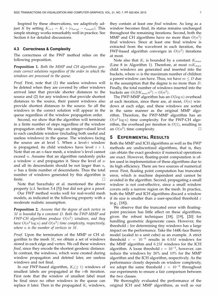
Model |F | Ratio of iteration numbersMMP/ICH FWP-MMP/FWP-ICH

Fertility 60,000 0.836 468/460 = 1.017Horse 96,965 0.714 775/772 = 1.004Bunny 144,036 0.680 865/911 = 0.950

Golfball 245,760 0.509 1478/1553 = 0.952Sphere 327,680 0.342 1286/1348 = 0.954

Armadillo 345,944 0.676 1931/1998 = 0.966Lucy 525,814 0.685 2286/2299 = 0.994

Gargoyle 700,000 0.695 2395/2446 = 0.979Blade 1,765,388 0.634 4086/3844 = 1.063

Dragon 4,000,000 0.788 13748/12387 = 1.110

TABLE 1Mesh complexity (face number |F |) and the ratios of the

number of iterations the algorithms need to converge for thepairs MMP, ICH and FWP-MMP, FWP-ICH.

0

50

100

150

200

250

300

0

2,000

4,000

6,000

8,000

10,000

12,000

14,000

16,000

18,000

Armadillo

FWP-MMP-SVG

ICH-SVG

Bunny Fertility Gargoyle Lucy Dragon

KSVG = 50Time (sec.)

Armadillo

FWP-MMP-SVG

ICH-SVG

Bunny Fertility Gargoyle Lucy Dragon

KSVG = 1000Time (sec.)

Fig. 8. The FWP method can improve SVG construction by afactor of 3 to 10. The parameter KSV G controls the accuracyof the computed geodesic distance. The higher KSV G, thesmaller the error, and the longer the time for constructing theSVG. Timing was measured on a single CPU core.

ble 1 shows, the FWP-CH and FWP-MMP algorithmspropagate the wavefronts at a similar pace and takeroughly the same number of iterations to converge.We believe that other window-based algorithms (ifany) can also fit into the FWP framework.

4) Improving the SVG technique. Saddle vertexgraph [9] is a sparse undirected graph that encodesthe geodesic information of a give mesh. With SVG,the geodesic distance can be computed efficientlyby Dijkstra’s shortest path algorithm. However, con-structing SVG is expensive, since one has to computeall direct geodesic paths2. In [9], the geodesic pathswere computed using the ICH algorithm, which istime consuming. For example, computing the exactSVG for the 144K-face Bunny model takes half an houron a single CPU core. Although SVG construction canbe significantly improved by parallel computing, theGPU implementation is non-trivial. In this paper, weshow that our CPU-based FWP method can be easilyadapted to compute SVG. Experimental results showthat our method can shorten the pre-computation timeby a factor of 3 to 10. See Figure 8.

2. A geodesic path is direct if it does not pass through any saddlevertices.

0

5,000

10,000

15,000

20,000

25,000

30,000

0 200 400 600 800 1,000 1,200 1,400 1,600 1,800

Iteration

Wavefront Size

K

0

1,000

2,000

3,000

4,000

5,000

6,000

7,000

8,000

9,000

10,000

0 100 200 300 400 500

Iteration

Wavefront Size

K

Fig. 9. K, the number of smallest-label windows usedin each iteration, is adapted to wavefront size. The ICHalgorithm has a similar performance as the MMP algorithm.

6 DISCUSSIONS

In this section we discuss three features as followsthat make the FWP method significantly improve thespeed of MMP/CH/ICH algorithms.

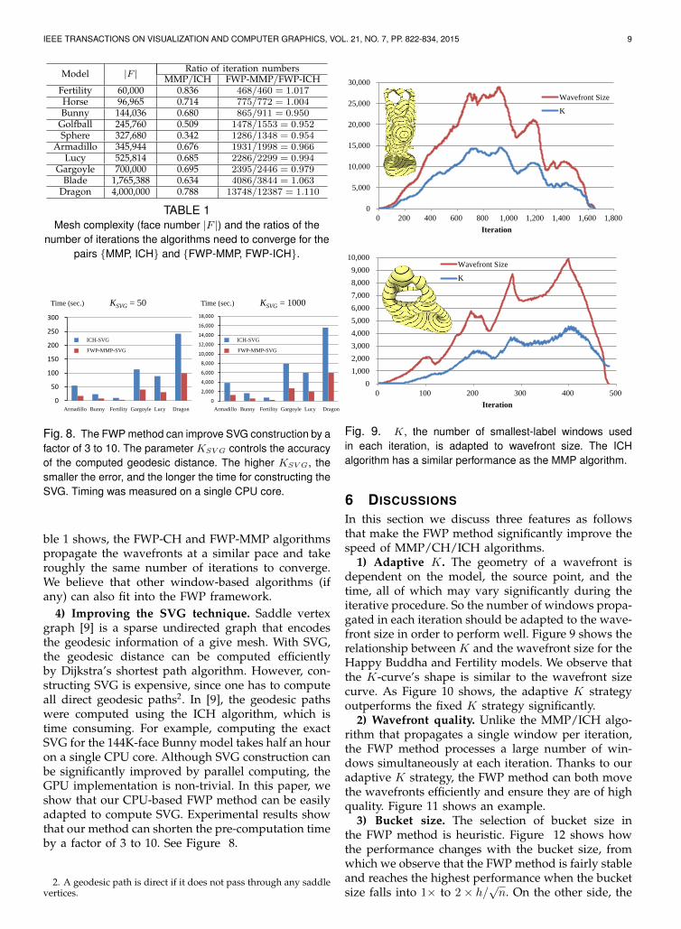
1) Adaptive K. The geometry of a wavefront isdependent on the model, the source point, and thetime, all of which may vary significantly during theiterative procedure. So the number of windows propa-gated in each iteration should be adapted to the wave-front size in order to perform well. Figure 9 shows therelationship between K and the wavefront size for theHappy Buddha and Fertility models. We observe thatthe K-curve’s shape is similar to the wavefront sizecurve. As Figure 10 shows, the adaptive K strategyoutperforms the fixed K strategy significantly.

2) Wavefront quality. Unlike the MMP/ICH algo-rithm that propagates a single window per iteration,the FWP method processes a large number of win-dows simultaneously at each iteration. Thanks to ouradaptive K strategy, the FWP method can both movethe wavefronts efficiently and ensure they are of highquality. Figure 11 shows an example.

3) Bucket size. The selection of bucket size inthe FWP method is heuristic. Figure 12 shows howthe performance changes with the bucket size, fromwhich we observe that the FWP method is fairly stableand reaches the highest performance when the bucketsize falls into 1× to 2× h/

√n. On the other side, the


0.00 0.05 0.10 0.15 0.20 0.25 0.30 0.35 0.40K

20

60

100

140

180

Tim

e (

s)

MMP

(x Kmax)

MMP

(x Kmax)

MMP

(x Kmax)

MMP

(x Kmax)

Armadillo Buddha Dragon Gargoyle

0.00 0.05 0.10 0.15 0.20 0.25 0.30 0.35 0.40K

40

80

120

160

200

Tim

e (

s)

ICH

(x Kmax)

ICH

(x Kmax)

ICH

(x Kmax)

ICH

(x Kmax)

Fig. 10. Fixing K has worse performance than the dy-namic K strategy. We measure the performance of the FWPmethod with various fixed K values, ranging from 1% to40% of Kmax. Each marker corresponds to the timing witha fixed K value and the optimal timing is highlighted in red.Clearly, theK values leading to the optimal performance varysignificantly among the test models. The dashed lines beloware the timing of the FWP method with adaptive K strategy.

(a) MMP (b) ICH

Fig. 11. Wavefront quality on the Dragon model. The priorityqueue based MMP and ICH algorithms produce high qualitywavefronts, however, the wavefronts are moving slowly dueto the expensive overhead. The FIFO queue based MMPand ICH algorithms have constant time overhead at eachiteration, however, their performance is very poor due tothe low quality wavefronts. Our FWP-MMP and FWP-CHalgorithm are able to propagate the wavefronts much fasterwithout compromising their quality. The horizontal axis is thenormalized timing and the vertical axis is the standard devia-tion of the wavefront. The smaller the standard deviation, thesmoother the wavefront, thus, the higher the quality it has.The close-up views show that the wavefronts of our methodhave similar quality to the wavefronts of the MMP and ICHalgorithms. The PCH algorithm is also macro, however, itswavefront quality is worse than ours.

Normalized Time

h / n

0.6

0.65

0.7

0.75

0.8

0.85

0.9

0.95

1

1.05

0 2 4 6 8 10

bunny lucy Armadillo 4kids buddha

Fig. 12. Performance changes with the bucket size. The x-axis shows different bucket sizes (by a multiple of h/

√n) and

the y-axis gives the normalized time (divided by the longestrunning time of each model).

curves shown in Figure 12 are U-shaped that meansboth too small and too large bucket size will lead torelatively bad performance.

7 COMPARISON

We compares the FWP method with other representa-tive geodesic algorithms, including MMP [2], ICH [7],PCH [8], FMM [13], [14], [22], the heat method [16]and the label correcting (LC) method [23]. We classifythese algorithms in two groups, i.e., macro and micro.A micro algorithm processes a single element (e.g.,a window in MMP/ICH or a triangle in FMM) periteration, whereas a macro algorithm processes multi-ple elements simultaneously. Table 2 summarizes thefeatures in these algorithms.

7.1 FWP vs. the Fast Marching MethodThe Fast Marching Method (FMM) [13] is a populartechnique for solving the boundary value problem ofthe Eikonal equation, ∇T = F (x, y), where F > 0is the front moving speed and T is the travel time.Solving the Eikonal equation with F ≡ 1 and T (s) = 0produces the polyhedral distance field at the source s.The FMM adopts a Dijkstra sweep and uses the factthat information only flows outward from the seedingarea. The FMM is flexible and can be applied to bothregular grids [13] and triangle meshes [14] with anO(n log n) time complexity, where the factor log n isdue to the administration of a priority queue.

To improve the speed of the FMM on regular grids,Yatziv et al. [22] suggested using a so-called untidypriority queue within the FMM. Their novel ideais to use the bucket sort technique together with aquantization that does not distinguish between thevalues of T within a small range. Therefore, each entryof the priority queue may contain multiple elements.Yatziv et al. showed that the number of elementsin each entry is O(1), and finding the element with


Method Domain Data Structure Overhead Space Complexity Time Complexity Type

CH

CH [3] triangle meshes FIFO queue O(1) O(n2) O(n2) microICH [7] triangle meshes priority queue O(logn) O(n2) O(n2 logn) microPCH [8] triangle meshes FIFO queue O(1) unbounded unbounded macroLC-CH triangle meshes FIFO queue O(1) Ω(n3) Ω(n3) micro

FWP-CH triangle meshes bucket & FIFO queue O(1) O(n2) O(n2) macro

MMPMMP [2] triangle meshes priority queue O(logn) O(n2) O(n2 logn) microLC-MMP triangle meshes FIFO queue O(1) Ω(n3) Ω(n3) micro

FWP-MMP triangle meshes bucket & FIFO queue O(logn) O(n2) O(n2 logn) macro

FMMFMM [14] regular grids priority queue O(logn) O(n) O(n logn) micro

triangle meshes priority queue O(logn) O(n) O(n logn) microYatziv’s regular grids untidy priority queue O(1) O(n) O(n) micro

FMM [22] triangle meshes untidy priority queue O(n logn) O(n) O(n2 logn) micro

TABLE 2Comparison of Dijkstra-like geodesic algorithms.

the minimal label also takes O(1) time. As a result,their algorithm has a linear run-time on regular grids.Although an error is introduced, it is of the sameorder as the local truncation error of the discretization,since the change of T values in a Dijkstra iteration isbounded on regular grids.

It is worth noting that the linear O(n) time com-plexity of Yatziv et al’s method does not hold ontriangle meshes, since it is not possible to boundthe change of T values on triangle meshes, whosetriangulation may be arbitrary. In fact, on trianglemeshes, the range of the change of T values dependson the triangulation, instead of the number of verticesn. Consider a very skinny triangle t whose longestside is of the same order of the model’s diagonal.Then the size of an entry (i.e., quantization step size)in the untidy priority queue must be big enough tocontain the longest side of t, meaning that this entrycontains O(n) triangles. Since finding the elementwith the minimal label takes O(n log n) time, the timecomplexity becomes O(n2 log n), which is much worsethan the original FMM.

Our experimental results also confirm that the per-formance of Yatziv et al’s FMM is highly depen-dent on the mesh triangulation. Moreover, the accu-racy of Yatziv et al’s method drops significantly onanisotropic meshes. See Figure 13(b). In terms of datastructure, note that the entry size in Yatziv et al’sFMM is triangulation dependent, while the bucketsize in the FWP method is fixed. Furthermore, theoverhead per window operation in Yatziv et al’s FMMis O(n log n) and in our method is O(1).

7.2 FWP vs. the Heat Method

The heat method [16] computes the geodesic distanceby solving a Poisson equation from the normalizedgradient of the heat flow. Based on standard numer-ical packages, it is easy to implement and highlyflexible to support a wide range of geometric do-mains, including grids, triangle meshes and pointclouds. Since the Laplacian matrix can be pre-factored,solving the Poisson equation takes only near-linear

1.0 1.5 2.0 2.5 3.0 3.5 4.0 4.5 5.0g

4

6

8

10

12

14

16

Tim

e (

s)

Armadillo

Buddha

Dragon

Gargoyle

Lucy

(a)

1.0 1.5 2.0 2.5 3.0 3.5 4.0 4.5 5.0g

0

1

2

3

4

5

avera

ge e

rror

(%)

Armadillo

Buddha

Dragon

Gargoyle

Lucy

(b)

(c) FWP result (d) FMM result

Fig. 13. (a) Yatziv et al.’s FMM, as a micro algorithm, itsperformance is sensitive to mesh triangulation. (b) Its av-erage numerical error increases significantly on anisotropicmeshes. (c) shows the FWP result and and (d) shows theFMM result with an average error 5.53%.

time. Below we compare the heat method and theFWP method in terms of accuracy and performance.

Accuracy. The accuracy of the heat method closelydepends on the heat diffusion time t. Theoretically, thetime approaching zero leads to the accurate solutionof geodesic distance. However, a tiny time t resultsin serious numerical issue. Crane et al. [16] observedthat the error-t plot is U-shaped and suggested t = h2

for common models, where h is the average edgelength. Similar to the fast marching method, theheat method computes a first-order approximationof geodesic distance. Thus, its results closely dependon the triangulation quality. Although the suggestedparameter t = h2 works fairly well on well-tessellatedmeshes, we observe that it leads to large error onanisotropic meshes. Figure 14 shows the results on theunit sphere with 200 longitude circles and 500 latitudecircles, which has 199,600 triangles and an anisotropy


0.00%

2.00%

4.00%

6.00%

8.00%

10.00%

12.00%

14.00%

16.00%

18.00%

0 20 40 60 80

Err

or

Step value

Maximal error

Average error

0.00%

5.00%

10.00%

15.00%

20.00%

25.00%

30.00%

0 1 2 3 4 5

Err

or

Step value

Maximal error

Average error

Fig. 14. The heat method controls the accuracy by thediffusion time t = λh2, where λ is the step value and h

is average edge length. Given the 199, 600-face unit spheremodel with the anisotropy measure g = 2.28, the defaultsetting λ = 1 produces a mean relative error 6.3%. Increas-ing the step value λ is helpful to reduce the mean error.For example, the mean error drops to 0.18% when λ = 80,however, the maximum relative error increases significantly.Given the 20, 000-face torus model with g = 2.36, the defaultsetting λ = 1 produces the best mean relative error 2.3%and the best maximum relative error 14.97%. Increasing ordecreasing the step value λ cannot help to reduce the errors.

measure g = 2.28. Setting t = h2 produces a meanrelative error 6.36%, comparing to the ground truthgeodesic distance computed by closed-form formula.Although taking a longer diffusion time smoothes thedistances and reduces the mean error, the maximalerror increases accordingly. Our method, in contrast,computes an accurate result with mean relative error0.00063% and maximal error 0.0044%. Figure 14 alsoshows the results on a 20, 000-face torus model withg = 2.36. The heat method obtains the best mean rel-ative error 2.3% and the best maximum relative error14.97% at λ = 1, while our method computes a moreaccurate result with mean relative error 0.00976% andmaximal error 0.1061%. In fact, as observed in [16]and [9], the discrete geodesic distances computed bythe MMP and CH algorithms converge to the smoothgeodesic distances at a quadratic speed, while theFMM and the heat method have only linear conver-

gence rate.Performance. As a pre-computation method, the

heat method has two steps: pre-computation (factor-ing the Laplacian matrix) and solving (recovering thedistances by solving a Poisson equation). Our FWPmethod is a direct approach, which is much slowerthan the heat method. However, as mentioned inSection 5, the FWP method complements the SVGmethod, since it reduces its pre-computation time. Itis noted that the SVG method has similar solvingperformance as the heat method and its accuracy ismuch higher. See Table 3.

7.3 FWP vs. the Parallel CH AlgorithmThe PCH algorithm [8] is a GPU-based parallel im-provement of the classic CH algorithm. Both the PCHand FWP algorithms propagate a large number ofwindows at each iteration and thus both are macro.However, they differ in two ways. First, the number Kof windows to be propagated in each iteration in FWPis time-dependent and adaptive to the wavefronts. AsFigure 11 shows, the wavefront quality of the FWPmethod is better than the PCH algorithm. Second,although the PCH algorithm performs well with real-world models, it is not possible to bind its space aswell as time complexities, which could be theoreticallyexponential. Our method, however, is theoreticallysound and produces at most O(n2) windows, leadingto provable time complexity of the FWP-MMP andFWP-CH algorithms. Computational results show thatour CPU-based FWP-MMP algorithm has a speedcomparable to PCH [8] (Table 3).

7.4 FWP vs. the Label Correcting MethodThe MMP and ICH algorithms propagate windowsin a continuous-Dijkstra fashion. Dijkstra’s algorithmtakes the node with the smallest label in a candidatelist C and is known as a label setting method, since thenode removed from the list is permanently labeledand never enters the list again. A label correcting(LC) method maintains a queue for the candidatelist C so that the selection of the to-be-processednode takes only O(1) time, at the expense of multipleentrances of nodes in C. Among many label correctingschemes, Bertsekas [23] observed that the SLF-LLL-THR algorithm performs extremely well in practice,significantly outperforming the original Dijkstra’s al-gorithm on real-world sparse graphs.

We implemented the SLF-LLL-THR strategy in theMMP and ICH algorithms and we refer to the LCbased methods as the LC-MMP and LC-CH algo-rithms. We compare the FWP-based algorithms withthe LC-based algorithms and we observe that theFWP method runs consistently faster than the LCmethods on all test models, the higher the meshresolution and anisotropy, the better the performanceimprovement of the FWP method to the LC method.


Model |F | Heat method SVG (K = 50)ICH FWP-MMP PCHPre-computation Solving Mean ErrorPre-computation Solving Mean Error FWP-MMP ICH

Armadillo 346K 1.75s 0.11s 0.90% 17.52s 54.4s 0.08s 0.14% 9.39s 3.43s 1.39sBunny 144K 0.72s 0.04s 0.83% 7.82s 23.63s 0.02s 0.12% 5.43s 2.0s 1.15s

Fertility 60K 0.22s 0.01s 1.81% 2.95s 10.14s 0.01s 0.14% 1.74s 0.79s 0.41sHorse 97K 0.35s 0.04s 0.72% 7.32s 15.91s 0.02s 0.12% 3.41s 1.38s 0.88sSphere 327K 4.92s 0.15s 0.19% 18.85s 51.29s 0.06s 0.10% 75.02s 16.56s 11.02s

TABLE 3Performance statistics on meshes with fairly good tessellation. The PCH algorithm was tested on an Nvidia GTX580 card

with 512 CUDA cores and all the other methods were implemented in single threaded C++ and tested on a PC with an IntelCore i7-2600 CPU (3.40 GHz). Both the heat method and the SVG method compute the approximate geodesic distances,

whereas the others are exact. For the heat method, we set the the diffusion time t = h2, where h is the average edge length.We construct a small-scale saddle vertex graph with K = 50 and report the mean relative error. The FWP-MMP based SVG

construction is 2 to 3 times faster than the ICH method.

0.5 1.0 1.5 2.0 2.5 3.0number of faces

1.0

1.5

2.0

2.5

3.0

3.5

4.0

4.5

Perf

orm

ance

Im

pro

vem

ent

×106×106×106

Lucy (FWP-MMP)

g=3.782g=1.944g=1.363

0.5 1.0 1.5 2.0 2.5 3.0number of faces

1.0

1.5

2.0

2.5

3.0

3.5

4.0

Perf

orm

ance

Im

pro

vem

ent

×106×106×106

Lucy (FWP-CH)

g=3.782g=1.944g=1.363

0.5 1.0 1.5 2.0 2.5 3.0number of faces

1.0

1.5

2.0

2.5

3.0

3.5

4.0

4.5

5.0

5.5

Perf

orm

ance

Im

pro

vem

ent

×106×106×106

Buddha (FWP-MMP)

g=3.463g=2.153g=1.469

0.5 1.0 1.5 2.0 2.5 3.0number of faces

1.0

1.5

2.0

2.5

3.0

3.5

4.0

Perf

orm

ance

Im

pro

vem

ent

×106×106×106

Buddha (FWP-CH)

g=3.463g=2.153g=1.469

Fig. 15. The FWP method is consistently faster than the LC-based method. The vertical axes show the ratio of the timingof the LC method to our method.

See Figures 15. Moreover, as a macro algorithm, theFWP method is more robust to mesh triangulation(using an anisotropic measure g) than the micro LCalgorithms.

Theoretically, the LC-based Dijkstra’s algorithm [23]does not have a time bound due to the heuristics usedfor determining the threshold. For the LC-based dis-crete geodesic algorithms, in Supplementary Materialwe construct a triangulation pattern so that the LCmethod produces at least Ω(n3) windows, leading toa Ω(n3) time complexity. In sharp contrast, our bucketdata structure and adaptive K strategy guaranteesan O(n2) window complexity accompanied with anO(n2 log n) time complexity for the FWP-MMP algo-rithm and an O(n2) time complexity for the FWP-CHalgorithm.

8 CONCLUSION

This paper presented a fast wavefront propagation(FWP) framework, which has the following advan-tages. First, as a macro algorithm, the FWP methodis less sensitive to mesh tessellation than the existingmicro (MMP/CH/ICH) algorithms. It is also a genericcomputational framework that enables the MMP andICH algorithms to propagate the wavefronts in a sim-ilar fashion. Second, the FWP method is theoreticallysound and has provable time and space complexity.The FWP-CH and FWP-MMP algorithms have O(n2)and O(n2 log n) time complexity, respectively. It isworth noting that the FWP-CH algorithm is the firstwindow-oriented algorithm that reaches the O(n2)lower bound while performing well in practice. Third,computational results show that the FWP-MMP algo-rithm can improve the speed of the MMP algorithmby a factor of 10 and the FWP-CH algorithm isalso 5 times faster than the ICH algorithm. Throughextensive evaluation presented in Supplemental Ma-terial, we confirm that the FWP-MMP algorithm is themost efficient serial and exact algorithm for computinggeodesic distances on triangle meshes. In the future,we will investigate the GPU-based parallelization ofthe FWP framework.

ACKNOWLEDGMENTS

We thank Keenan Crane for his code of the heatmethod. The models are courtesy of Aim@Shape andStanford University. This work was supported bythe Natural Science Foundation of China (61322206,61432003, 61272228), the National Basic ResearchProgram of China (2011CB302202), TNList Cross-discipline Foundation and Beijing Higher InstitutionEngineering Research Center of Visual Media Intel-ligent Processing and Security, and Singapore Min-istry of Education Grants (MOE2013-T2-2-011 andRG40/12).


REFERENCES[1] P. Bose, A. Maheshwari, C. Shu, and S. Wuhrer, “A survey

of geodesic paths on 3D surfaces,” Computational Geometry,vol. 44, no. 9, pp. 486–498, 2011.

[2] J. S. Mitchell, D. M. Mount, and C. H. Papadimitriou, “The dis-crete geodesic problem,” SIAM Journal on Computing, vol. 16,no. 4, pp. 647–668, 1987.

[3] J. Chen and Y. Han, “Shortest paths on a polyhedron,” inProceedings of the Sixth Annual Symposium on ComputationalGeometry. ACM, 1990, pp. 360–369.

[4] Y.-J. Liu, D. Fan, C. Xu, and Y. He, “On discrete geodesics:tight bound and triangle anisotropy,” Submitted for publication,2015.

[5] V. Surazhsky, T. Surazhsky, D. Kirsanov, S. J. Gortler, andH. Hoppe, “Fast exact and approximate geodesics on meshes,”in ACM Transactions on Graphics, vol. 24, no. 3. ACM, 2005,pp. 553–560.

[6] Y.-J. Liu, “Exact geodesic metric in 2-manifold triangle meshesusing edge-based data structures,” Computer-Aided Design,vol. 45, no. 3, pp. 695–704, 2013.

[7] S.-Q. Xin and G.-J. Wang, “Improving Chen and Han’s algo-rithm on the discrete geodesic problem,” ACM Transactions onGraphics, vol. 28, no. 4, p. 104, 2009.

[8] X. Ying, S.-Q. Xin, and Y. He, “Parallel Chen-Han (PCH) al-gorithm for discrete geodesics,” ACM Transactions on Graphics,vol. 33, no. 1, pp. 9:1–9:11, 2014.

[9] X. Ying, X. Wang, and Y. He, “Saddle vertex graph (SVG):a novel solution to the discrete geodesic problem,” ACMTransactions on Graphics, vol. 32, no. 6, pp. 170:1–170:12, 2013.

[10] S.-Q. Xin, X. Ying, and Y. He, “Constant-time all-pairs geodesicdistance query on triangle meshes,” in Proceedings of the ACMSIGGRAPH Symposium on Interactive 3D Graphics and Games,2012, pp. 31–38.

[11] ——, “Efficiently computing geodesic offsets on trianglemeshes by the extended xin-wang algorithm,” Computer-AidedDesign, vol. 43, no. 11, pp. 1468–1476, 2011.

[12] S.-Q. Xin, Y. He, and C.-W. Fu, “Efficiently computing exactgeodesic loops within finite steps,” IEEE Trans. Vis. Comput.Graph., vol. 18, no. 6, pp. 879–889, 2012.

[13] J. Sethian, “A fast marching level set method for monotonicallyadvancing fronts,” Proceedings of National Academy of Sciences,vol. 93, pp. 1591–1595, 1996.

[14] R. Kimmel and J. Sethian, “Computing geodesic paths onmanifolds,” Proceedings of National Academy of Sciences, vol. 95,pp. 8431–8435, 1998.

[15] S.-Q. Xin, D. T. Quynh, X. Ying, and Y. He, “A global algorithmto compute defect-tolerant geodesic distance,” in SIGGRAPHAsia 2012 Technical Briefs, 2012, p. 23.

[16] K. Crane, C. Weischedel, and M. Wardetzky, “Geodesics inheat: A new approach to computing distance based on heatflow,” ACM Transactions on Graphics, vol. 32, no. 5, p. 152, 2013.

[17] K. Hildebrandt, K. Polthier, and M. Wardetzky, “On the con-vergence of metric and geometric properties of polyhedralsurfaces,” Geometriae Dedicata, vol. 123, no. 1, pp. 89–112, 2006.

[18] Y.-J. Liu, Q.-Y. Zhou, and S.-M. Hu, “Handling degeneratecases in exact geodesic computation on triangle meshes,” TheVisual Computer, vol. 23, no. 9-11, pp. 661–668, 2007.

[19] H. Edelsbrunner and E. P. Mucke, “Simulation of simplicity:A technique to cope with degenerate cases in geometric al-gorithms,” ACM Trans. Graph., vol. 9, no. 1, pp. 66–104, Jan.1990.

[20] C. K. Yap, “A geometric consistency theorem for a symbolicperturbation scheme,” in Proceedings of the Fourth Annual Sym-posium on Computational Geometry, ser. SCG ’88, 1988, pp. 134–142.

[21] Z. Zhong, X. Guo, W. Wang, B. Levy, F. Sun, Y. Liu, andW. Mao, “Particle-based anisotropic surface meshing,” ACMTrans. Graph., vol. 32, no. 4, pp. 99:1–99:14, 2013.

[22] L. Yatziv, A. Bartesaghi, and G. Sapiro, “O(N) implementa-tion of the fast marching algorithm,” Journal of ComputationalPhysics, vol. 212, no. 2, pp. 393–399, 2006.

[23] D. P. Bertsekas, Network Optimization: Continuous and Discretemodels. Athena Scientific Belmont, 1998.

ieee transactions on visualization and …cg.cs.tsinghua.edu.cn/people/~yongjin/fwp-tvcg.pdf ·...

Documents