ieee transactions on visualization and computer …chengu/publications/timedep_vfdsurf.pdf · ieee...

IEEE TRANSACTIONS ON VISUALIZATION AND COMPUTER GRAPHICS, VOL. ?, NO. ?, ? 2011 1

Design of 2D Time-Varying Vector FieldsGuoning Chen, Member, IEEE, Vivek Kwatra, Li-Yi Wei, Charles D. Hansen, Senior Member, IEEE, and

Eugene Zhang, Member, IEEE,

Abstract—Design of time-varying vector fields, i.e., vector fields that can change over time, has a wide variety of important applicationsin computer graphics. Existing vector field design techniques do not address time-varying vector fields. In this paper, we present aframework for the design of time-varying vector fields, both for planar domains as well as manifold surfaces. Our system supports thecreation and modification of various time-varying vector fields with desired spatial and temporal characteristics through several designmetaphors including streamlines, pathlines, singularity paths, and bifurcations. These design metaphors are integrated into an element-based design to generate the time-varying vector fields via a sequence of basis field summations or spatial constrained optimizations atthe sampled times. The key frame design and field deformation are also introduced to support other user design scenarios. Accordingly,a spatial-temporal constrained optimization and the time-varying transformation are employed to generate the desired fields for thesetwo design scenarios, respectively. We apply the time-varying vector fields generated using our design system to a number of importantcomputer graphics applications that require controllable dynamic effects such as evolving surface appearance, dynamic scene design,steerable crowd movement, and painterly animation, many of which are difficult or impossible to achieve via prior simulation-basedmethods. In these applications, the time-varying vector fields have been applied as either orientation fields or advection fields to controlthe instantaneous appearance or evolving trajectories of the dynamic effects.

Index Terms—time-varying vector fields, 2D vector fields, vector field design, dynamic effects for surfaces

F

1 INTRODUCTION

V ECTOR field design is a fundamental component for avariety of graphics applications such as remeshing [1],

[33], texturing [20], [13], [23], [31], [41], [46], and non-photorealistic rendering [16], [17]. The paramount importanceof vector fields in these applications has invoked a line ofcomprehensive study on the techniques of vector field designon surfaces [6], [8], [34], [51]. Nonetheless, prior research haspaid little attention to the more natural and general applicationsof vector field design to modeling dynamic effects, such asfluid animation [35], [36], crowds [4], [29], shape deforma-tion [45], and video editing [18]. This is in part due to the factthat such dynamic systems are usually time-varying (or time-dependent), with the additional time dimension significantlyincreasing the complexity of the possible dynamics in thevector fields. In addition, there is no existing theory forthe characterization of time-varying vector fields comparedto the well-defined feature characterization of static vectorfields upon which the design techniques are built. This paper,for the first time, systematically studies the design of time-varying vector fields on two-dimensional manifolds, such asthe applications, the taxonomy of the vector fields (orientation,advection), the requirements, and appropriate techniques.

• Guoning Chen and Charles Hansen are with Scientific Computing andImaging Institute, University of Utah, Salt Lake City, UT 84112.E-mail: {chengu,hansen}@sci.utah.edu

• Vivek Kwatra is with Google Inc., Mountain View, CA 94043.E-mail: [email protected]

• Li-Yi Wei is with Microsoft Research, Redmond, WA 98052-6399, and TheUniversity of Hong Kong, Pokfulam, Hong Kong.

• Eugene Zhang is with Oregon State University, Corvallis, OR 97331.E-mail: [email protected]

1.1 Requirements

For most of graphics applications involving dynamic effects,there are a number of requirements on the underlying time-varying vector fields and how they are modeled.

First, the designed time-varying vector fields should pre-serve temporal coherence to guarantee the smooth transitionof dynamic effects that they are driving. This is a fundamentalrequirement for achieving a visually pleasing animation.

Second, the obtained time-varying vector fields can be phys-ically plausible or implausible, incompressible or compress-ible, in order to satisfy the different requirements of specificapplications. For instance, practitioners in fluid dynamics oftenrequire incompressible flows, while animators may seek formore flexible vector fields for the dynamic effects with volumechange such as crowd simulation. Any vector field systemneeds to be able to handle general time-varying vector fieldswith such diverse properties.

Third, the time-varying vector fields are designed to eithercontrol the evolution of the instantaneous appearance of certaingraphical primitives (e.g. the sizes and orientations of thetexture and brush strokes) or advect certain objects (e.g. flowparcels) over time, in order to control different aspects of thedynamic effects. A vector field design system should facilitateboth types of vector fields.

Fourth, the design system for the time-varying vector fieldsshould provide the user an intuitive and flexible interface tosupport the modeling of various flow behaviors. In addition, anumber of different modeling approaches should be supported.Specifically, there are a few possible situations during themodeling of a time-varying vector field that a user mayencounter. 1) The user wishes to design the detailed localbehavior of the flow over time. 2) The user cares about the


Fig. 1: This figure shows the pipeline of the presented design system for 2D time-varying vector fields. First, the user specifies the desiredflow behaviors in the forms of spatial-temporal constraints. The system then produces a time-varying vector field that matches the constraints.The obtained field is then applied to the computer graphics applications to create various dynamic effects. Here, we apply the obtained fieldsto produce painterly animation from a single image. Note that we use the created time-varying vector field to orient and move the brushstrokes in the lower part of the image to achieve an artistic water wave effect: the vortex rotates, moves and changes its characteristics, thensplits into two vortices at the end. Please see the accompany video for this animation. The inset plot shows the changes of the consecutiveinstantaneous fields in terms of the total variance of the vector values in the space.

exact states of the flow at only certain times and would likethe system to generate the rest of the field. 3) The user isgiven a static vector field, and tries to deform it to make up asequence of time-varying vector field as people do for meshdeformation. A properly devised design system should be ableto accommodate these scenarios.

1.2 Our MethodIn order to develop a design system for time-varying vectorfields to satisfy the aforementioned requirements, we proposea design framework which is based on the discretization ofthe time-varying vector fields in the time dimension andconsider them as the sequences of static vector fields withslow changes over time. This philosophy is based on anobservation that solutions to the time-varying vector fieldsconverge to families of solutions of the instantaneous vectorfields as the rate of temporal change in the vector field goes tozero, which preserves temporal coherence and helps achievesmooth transition of the dynamic effects. This observation isalso a fundamental assumption when developing bifurcationtheory for time-varying vector fields [11]. With this temporaldiscretization, we are able to adapt the previously developedtools for static vector field design to time-varying vector fieldswith the desired instantaneous dynamics.

To enable the creation of various flows, we provides the userwith the ability of modeling the following flow properties:

1) a snapshot of the flow at a given time, 2) the path of aparticle in the domain, 3) the path of a singular feature, and4) the interaction of the features of interest. These features inturn reflect important flow characteristics, such as the solutionof the dynamical system at a given time, the trajectories ofthe flow parcels, and how the flow parcels interact over time.These flow characteristics can be described by streamlines,pathlines, singularity paths, and bifurcations, respectively.They sufficiently describe the local flow behavior in space andtime, and are capable of creating time-varying vector fields thatare used to align or advect the graphical primitives as required.The former type of vector field is referred to as an orientationfield and the latter an advection field. We provide the designmetaphors for the user to model these flow characteristics.Specifically, we present the first technique that allows theuser to prescribe bifurcations, a unique type of phenomenanot present in static fields.

To support the required design scenarios, we introduce threedistinct field design approaches. Specifically, the modelingof the local flow behaviors is supported by the time-varyingdesign elements extracted from the user specified flow charac-teristics. A basis field summation or a constrained optimizationis performed to generate the instantaneous vector field ata given time based on the instantaneous characteristics ofthe elements. Key frame design is employed to support thecase when a user only provides the instantaneous fields at


the desired times. A spatial-temporal Laplacian relaxation isproposed to generate the rest of the sequence. Time-varyingtransformation is used when an initial static field is deformedover time to generate a time-varying vector field.

The combination of the proposed design metaphors and gen-eration techniques has led to a design system which takes theuser input and generates a time-varying vector field using oneof the generation approaches according to the selected designapproach. The system also enables the user to further modifythe obtained vector field through local topological editing.The generated time-varying vector fields can be applied to anumber of important computer graphics applications to achievevarious dynamic effects including producing artistic fluideffects over static images, steering 2D crowds, controlling fieldanimations, and time-varying effects of surface appearance.

2 RELATED WORK

Vector field design refers to the creation of a continuous vectorfield on a manifold that respects user specified or application-dependent constraints. Most existing work focuses on a staticvector field. Depending on the goals, there are two differentclasses of vector field design techniques: One is non-topologybased; the other is topology based.

Non-topology based methods: Non-topology based methodsdo not address vector field topology [15] explicitly. The vectorfield design tools in the early graphics applications, such astexture synthesis [41], [46], fluid simulation [35], [36], andvisualization [43], are the examples of this category. Otherapplications, such as non-photorealistic rendering [16], [17],remeshing [1], and parameterization [33], also employ vectorfield design respectively. Most of these applications requireonly the direction information of the input vector fields, andhence a simple design functionality for the vector fields.However, the user has little control of unwanted singularitiesin the field that often leads to visual artifacts.

Topology-based methods: Topology-based approaches allowthe user to control the number and positions of singulari-ties [44], [51], [8] or the topological graph explicitly [37].More general N-way rotational symmetry field design has alsobeen studied by Palacios and Zhang [27], Ray et al. [34],and Lai et al. [21]. Recently, Crane et al. [6] present atechnique which allows arbitrary prescription of singularitiesand constraints on the fields.

Time-varying methods: Most of the above work concernsonly time-independent (i.e. static) vector fields. On the otherhand, many applications produce time-varying vector fieldsduring execution without providing the user an effective inter-vening interface, such as fluid simulation [35], crowd anima-tion [39], [29], shape deformation [45], hair modeling [10],and video editing [50]. This has restricted the achievableeffects. Wejchert and Haumann [47] introduce the idea offlow design to create controllable aerodynamics animation.The modeled field is steady and needs to be combinedwith physically-based simulation to generate aerodynamicsanimation. To achieve time-dependent control, the user exertsexternal force to the system as the work by Stam [35],

[36]. However, simulation is expensive and hard to control.In addition, simulation is incapable of generating physicallyimpossible artistic fluid flow effect. Pighin et al. [30] has ac-complished a closely related work. They introduce an advectedradial basis function to model and edit flows as well as aninteractive pathline editing interface. Compared to their work,our techniques enable the user to create more general 2D vec-tor fields than those incompressible flows. Recently, Kagaya etal. [18] present a simple design interface to control the time-varying tensor fields for the temporarily coherent painterlyrendering of videos. Xu et al. [49] describe a technique for fastdynamic design of vector fields. These fields need not preservetemporal coherence. Ma et al. [24] propose a motion fieldsynthesis technique which enables the user to generate artisticflow effects. However, the method only generates detailedmotion vectors and relies on a predetermined low resolutiondynamic vector field for synthesis. To that end, we are notaware of any work on the design of time-varying vector fieldsfor the general purpose of graphics applications.

3 OVERVIEWIn this section, we provide a brief description of how ourframework assists the design of a time-varying vector field.First, the user provides a number of specifications on thedesirable characteristics of the field. These include:

flow descriptors examples

Streamline, for the controlof the flow geometry at acertain time frame and mostuseful for the design of ori-entation fieldsPathline, for the descrip-tion of movements of spe-cific particles across spaceand time (appropriate for ad-vection fields)Singularity path, for therepresentation of the trajec-tory of the singular featuresover space and time (usefulfor orientation fields)Bifurcation, for the descrip-tion of the collisions or splitsof different singular featuresover space and time (usefulfor orientation fields)

These characteristics depict diverse flow behaviors whichcan be observed in many dynamic applications. For instance,in texture synthesis and painterly rendering, the user oftenwishes the texture patches and brush strokes to be oriented ina certain way. An orientation field can be created to achievethat with the desired instantaneous flow patterns prescribedby the user specified streamlines. In crowd simulation, theuser would like to steer a group of pedestrians to followcertain route. This is similar to specifying a path for thesepedestrians. An advection field generated from the specified


pathline can be applied to accomplish that (see Figure 16). Inmeteorological animation design, the user may create the effectof two storm systems moving toward each other and eventuallycolliding (see Figure 9). This can be done by controlling themovement (singularity paths) and interaction (bifurcation) ofthe two vortices in a time-varying vector field.

Note that for most graphics applications shown in this paper,instantaneous appearance is often a bigger goal than the exactpath of a particle. For the rest of the paper, we will assumethe designed fields serve as orientation fields except for theapplication of crowd simulation where the pathline design isused to generate an advection field. Nonetheless, for mostexamples the orientation fields are also used to advect thegraphical primitives over time to achieve the moving effect.

The overall pipeline of our system is as follows (shown inFigure 1). First, according to the selected design scenario, theuser specifies a number of constraints. For key frame designand field deformation, the focus is on the creation of someinstantaneous (static) fields. As such, specifying streamlinesand the singularities is sufficient. A streamline can be specifiedusing the drawing tool of our system. Our system will computethe tangent vectors at the sample positions as the constraints.For element-based design, pathlines, singularity paths, andbifurcations can be used. In particular, for a pathline, besidescomputing the tangent vectors at the sampled positions, thetemporal value for each sample point is required from theuser (Section 5.1). The user is also responsible to provide thetype of a singularity path (source, sink, or saddle), representedas a time-varying Jacobian. To specify a bifurcation, the usercan describe a template function (Section 5.1) that will lead tothe desired bifurcation. Note that in our paper we only handlesaddle-node bifurcation where a node is either a source orsink. Figure 2 provides some examples on how the users canspecify these flow descriptors with our system.

Once the constraints have been specified, our system gener-ates a time-varying vector field by using the basis field sum-mation (Section 5.2), constrained optimization (Sections 5.3and 6.1), or time-varying transformation (Section 7) accordingto the selected design method. The resulting field is analyzedwith singularities and bifurcations extracted. The user then hasthe ability to specify additional constraints or perform localtopological editing in the form of singularity and bifurcationmovement or cancellation. This process continues until theuser is satisfied (Section 8).

In the next section, we will provide the mathematicaldefinitions for the aforementioned flow characteristics.

4 TIME-VARYING VECTOR FIELDS

In this section, we briefly review the mathematical definitionsof the important concepts of time-varying vector fields, whichwill facilitate our later design tasks.

Streamlines and Pathlines: We consider a 2-manifold M. Atime-varying vector field V is a map V : M×R→M, whichcan be expressed as a differential equation dx

dt = V (x; t). Thesolution of it given an initial state p0 = (x0; t0) is x(b) = p0 +∫ b

0 V (x(η); t+η)dη , which is referred to as a pathline. It is thetrajectory of the particle under V . The vector field V (x; tc) is

Fig. 2: Our user interface showing different design metaphors: (a)streamline, (b) pathline, (c) singularity path, and (d) bifurcation. Astreamline is specified at a particular time as a 2D curve. A pathlinecan be provided either in the 2D domain with the starting and endingtime information or directly in the spatial-temporal domain (see theinset of b). Similarly, a singularity path can be designed in either2D domain with the birth and death times or in the spatial-temporaldomain (see the inset of d). A bifurcation is prescribed as a pointin the spatial-temporal domain with the coordinate, scaling, andorientation information.

an instantaneous vector field of V at time tc, which is static.The solution from pc = (xc; tc) constrained in V (x; tc) is astreamline, and x(b) = pc +

∫ b0 V (x(η); tc)dη .

Instantaneous Topology: The topology of V (x; tc) is referredto as the instantaneous topology of V at tc. It consists ofsingularities, periodic orbits, and their connectivity [3] andconveys the qualitative information of V (x; tc). This informa-tion has been applied to guide the creation and control ofstatic vector fields [3], [8], [44], [51]. It has been shownthat analyzing and tracking instantaneous features can providemore information for graphics applications than the space-time topology defined based on pathlines which is typicallyfeatureless [38]. Therefore in the rest of the paper, we willmake use of the notion of instantaneous topology to discussthe structural evolution of a time-varying vector field. Also,we focus on singularities only as they are more relevant to thepresent graphics applications.

Singularities and Singularity Paths: A point p is calleda singularity of V (x; tc) if V (p; tc) = 0. We are interestedin the isolated singularities in the field, each of which canbe enclosed by a compact neighborhood containing no othersingularities. The type of each singularity is determinedby the flow characteristics within this neighborhood. Thelinearization of V (x; tc) about p results in a 2× 2 matrix


Fig. 3: This figure shows an example of saddle-node bifurcation inan orientation vector field. The creation of a pair of saddle and sinkcauses the break of texture structure on the back of the bunny. Notethat we sample the two frames before (left column) and after (right)the bifurcation point to reveal the discontinuity.

tj0-1 tj0 tj0+1

saddle source unstable singularity

(bifurcation point) �

instantaneous vector fields

Fig. 4: This example demonstrates a saddle-source cancellationbifurcation. The directional curves illustrate the flow behavior. Twosingularities are shown in the left at t j0−1. They move towards eachother when t increases and collide at t j0 (middle). The two singular-ities are canceled after they meet, which results in a singularity-freevector field at t j0+1 (right).

DV (p) =(

∂vx/∂x ∂vx/∂y∂vy/∂x ∂vy/∂y

)(called Jacobian) which has

two (potentially complex) eigenvalues σ1 + iµ1 and σ2 + iµ2.If σ1 6= 0 6= σ2,then p is called a hyperbolic singularity. Theyare the stable structures w.r.t perturbation compared to thoseunstable ones, such as centers. Observe that on a surface thereare three types of hyperbolic singularities: sinks σ1,σ2 < 0,saddles σ1 < 0 < σ2, and sources 0 < σ1,σ2. Each singularityhas a life span [ts, te] (ts, te ∈ R) where ts represents the timeof its birth and te is the time of its annihilation. The curveconnecting each position of the singularity during its life spanis called a singularity path. We assume the type of a singularitydoes not change during its life span.

Bifurcations: The birth and annihilation of singularities implythe change of the topological structural of the vector field.We refer to this qualitative change as the bifurcation and theplaces where these changes occur as the bifurcation points.Bifurcation is an important event in time-varying vector fields.In many graphics applications involving time-varying vectorfields, bifurcations can lead to the structural changes of certaingeometry or properties, such as the splitting and merging ofvortices in fluid animation. In some cases, these structuralchanges may cause visual artifacts. Figure 3 shows an examplewhere the break of texture structures induced by the bifurca-tions of the underlying vector field causes visual discontinuity

in the animation. Therefore, studying bifurcations and develop-ing effective techniques to control them is necessary from theapplication perspective. The rigorous definition of bifurcationis beyond the scope of this paper. Interested readers can finda more comprehensive introduction of the bifurcation theoryin [11]. Consistent with our focus on singularities, in this paperwe discuss only the local bifurcations, such as saddle-node(fold) bifurcation and its inverse bifurcation which refers to theannihilation of sink/source and saddle pairs. Figure 4 illustratesa saddle-source bifurcation where a source with Poincare index1 and a saddle with index -1 move towards and finally canceleach other over time. This bifurcation can be formulated asfollows [11].

V ((x,y); t) =(

t + x2

y

)(1)

while a saddle and sink creation can be formulated as follows,

V ((x,y); t) =(

t− x2

−y

)(2)

The change of the type of a singularity also corresponds toa transcritical bifurcation, for instance, sink→center→source,and vice versa. When this occurs, we consider a new singu-larity is born while the old one is eliminated.

With these concepts, we next describe how we support thethree different design scenarios as introduced in Section 1. Wefirst describe the setting of our computation domain.

Computation Domain: We consider a sub-domain DX =(X ; t) where DX ⊂ M × R is a spatial-temporal domain.

Ti

Ti�tj

�tj-1

tX is a triangulation of a 2D curvedsurface embedded in 3D, and t ∈ [0,1]is the time parameter. For representingand storing the field, we discretize tevenly. We denote these discretely sampled values as {t j}.We then compute and store the instantaneous fields at thesediscrete times {t j} in order. In each instantaneous field, vectorvalues are sampled at the vertices of the triangulation X . Theinset figure shows such a configuration. For a planar domain,we use a free-form boundary. Along t, we assume the time-varying vector field in Dx is a portion of the time-varyingfield with t ∈ (−∞,∞). Other boundary conditions of t can beemployed, such as a periodic boundary conditions often usedin fluid simulation [35].

Note that in order to enable more flexible speed control ofthe final animation sequences, the parameter t has a linearrelation with the physical time, that is, c ·dt (c ∈ R+) will bethe actual time interval when applying the created field to thetarget applications.

Interpolation scheme: We assume that the vector field isdefined on the vertices of the mesh domain. In space X , thevector values within a triangle is computed using the paralleltransport technique of Zhang et al. [51]. Along the parametert dimension, we employ a similar interpolation techniqueproposed by Tricoche et al. [40] to guarantee the linearity overt. In particular, the vector value of a sample point p in-betweentwo frames can be computed using linear interpolation of thetwo values at p at the two frames.


5 ELEMENT BASED DESIGN

In this section, we describe how we support the design of localspatial and temporal behaviors of the flow through a number ofdesign elements that can be extracted from the user specifiedflow characteristics. These design elements are later combinedto generate a time-varying vector field.

5.1 Design Elements

Our system supports the following design elements.

Singular Elements:Modeling singular elements is an essential functionality

for vector field design. We extend the singular elements inthe static field design [51] to our spatial-temporal setting.Specifically, we denote a singular element as S(J,P(t),M(t)),where J is the Jacobian that defines the selected type of the sin-gular element, P(t) represents the path of the singular elementover time, and M(t) is the affine transformation matrix (i.e.scaling and rotating) that is exerted on the element along P(t).

Bi(x;t)=0�t0

(x0;t0)

y

x tj �tn�

(xj;tj)(xn;tn)

�0

�j�n

...... ......

t

y

x

Fig. 5: Singularity path.

We assume J is fixed alongP(t). P(t) is derived from auser specified path (Figure 5).In particular, after the usersketches the path of a singu-lar element, a Hermite splinecurve is fitted to it to forma smooth path P(t). M(t) isinitialized as an identity ma-trix and can be modified alongP(t). Given a time tc, M(tc) =(

sx(tc) 00 sy(tc)

)R(θ(tc)) where sx(tc) is a x scaling, sy(tc)

a y scaling, and R(θ(tc)) a rotation centered at P(tc). The userspecifies a number of M(ti) at the desired times ti. M(t) canbe computed through linearly interpolating sx, sy and θ at tiand ti+1 where ti < t < ti+1.

P(t) starts and ends at t = 0 and 1 by default. If it startsor ends in between, a certain bifurcation is induced, whichin turn involves another singularity with opposite Poincareindex. In design, this can be achieved by intersecting the twosingularity paths (by definition in Section 4). At the bifurcationpoint where the two paths intersect, the local Jacobian isdegenerate, while the Jacobian of the rest of the field is not. Inaddition, after (cancellation) bifurcation, the field is singularityfree (see Figure 3 (right)). Therefore, local control of theJacobians through the singularity paths to their bifurcationpoint is insufficient to guarantee a smooth and non-degeneratefield. In the following, we introduce the bifurcation elementsthat can reduce the burden of the local and global control ofthe Jacobians from the user.

Bifurcation Elements: Recall that we are concerned withsaddle-node bifurcations in this paper. Equations 1 and 2are two normal forms that define a saddle-node bifurcationat position (0,0;0) in domain X (i.e. a bifurcation element).Specifically, equation 1 induces a saddle-source cancellationand equation 2 defines a saddle-sink creation. During design,the user prescribes the position, (x0,y0; t0), of a bifurcation

with the desired type in domain X . Thus, we replace x= x−x0,y = y− y0, and t = t − t0 in equations 1 or 2 to place thebifurcation elements in the right position. Further, a usermanipulated transformation can be exerted to scale the rangeof the bifurcation in both space and time, and re-orient anaxis (a straight line in this case) to control where and howthe bifurcation occurs along the axis. Figure 6 provides anexample where the user inserts a number of bifurcations.

Fig. 6: A number of bifurcations are inserted using the Equations 2(red), 1 (green).

These bifurcation elements enable the user to insert bifur-cations through templates (i.e. the bifurcation normal forms)with guaranteed smooth transition in space and time. However,it does not allow the modification of the paths of the involvingsingularities. More intuitive and flexible design metaphor forbifurcations is much desired and should be included in thefuture work.

Regular Elements:In static field design, a regular element is useful in providing

the translation or advection direction for a particle located at apoint and related to streamlines. In the design of time-varyingvector fields, this element is tightly linked to pathlines.

We define a regular element as R(V (t),P(t)) where P(t) isa prescribed pathline and V (t) is the tangent direction at P(t)in space at a time t.

Consider a user specified pathline curve whichconsists of the positions of a particle p fromts to te (te ≥ ts), denoted by

⋃tts(p(s)). Assume

m sample points, pi, along the curve are taken.

Fig. 7: Pathline example.

A Catmull-Rom splineP(t), is computed with{pi} as the controlpoints. The spline curveis densely sampled asthe set of evenly spacedpoints {sp j}. AssumeK is the number ofsample points on the spline curve and N is the number oftime samples. We set K > 4N for a smooth representationsuch that V (ti) = (sp j− sp j−1), a good approximation of thetangent direction, is placed at P(ti) where ti ∈ [0,1] is the ith

sampled time (see Figure 7). To reduce user input, a uniformsampling, ti = ts + i× (te− ts)/(N−1) can be used. However,this is not required. sp j and sp j−1 are the points that encloseP(ti) on P(t).

Because of the cumulative numerical integration error, thecomputed pathline starting from P(0) following the generatedflow is typically deviated from the prescribed P(t). To resolve


that, instead of using conventional regular elements, we makeuse of the attachment elements introduced in [3], whichguarantee the obtained pathline converging to the desired one.The following formula describes an attachment element thathas a vector value of (1,0) at (x0,y0).

V (x,y) =(

1c(y− y0)

)(3)

5.2 Basis Fields SummationIn order to generate a time-varying vector field from the userspecified elements described above, a basis field summationcan be used which has been applied to static field design [47],[44], [51]. We extend this basis field summation to take intoaccount the design elements with time-varying characteristicsintroduced in the previous section. Specifically, the basis fieldgenerated by a singular element at time t has the form:

Vi(x; t) = e−d‖x−pi(t)‖2MTi (t)JiMi(t)

(x− xpi(t)y− ypi(t)

)(4)

where pi(t) = (xpi(t),ypi(t)) is the position of the singularelement at time t along the path Pi(t), and Mi(t) is thetransformation acting on Ji. The basis field for a regularelement given time t has the form

Vi(x; t) = e−d‖x−pi(t)‖2Vi(t) (5)

The basis field for an attachment element at t is

Vi(x; t) = e−d‖x−pi(t)‖2MTi (t)

(1

c(y− ypi(t))

)(6)

A bifurcation elements generate the following basis field.

Vi(x; t) = e−d‖x−pi(t)‖2Vbi(Mi

(x− xpi(t)y− ypi(t)

); t− ti) (7)

where (pi(ti); ti) is the position at which the ith bifurcationoccurs and Mi is a transformation matrix specified by user toorient the moving direction of the two singularities. Vbi is oneof the bifurcation normal forms (e.g. equations 1 and 2).

Accordingly, the obtained global time-varying vector fieldis the sum of these individual basis fields.

V (x; t) = ∑i

Vi(x; t) (8)

Figure 8 provides a time-varying vector field generatedusing the element-based design and the basis field summation.Note that we extended the design elements to the spacetime domain from their static counterparts. Each design el-ement at a given time acts as a static one except for abifurcation element that is defined by its normal form. Assuch, the basis field summation is largely the same as itsstatic counterpart. Consequently, the issue of the cancellationof an element by the influence of its nearby elements canarise. To relieve that, we can use a sharper fall off func-tion with a larger d or require the design elements to beplaced sufficiently far apart to reduce their mutual influence.Another possible solution is to extend the work of Turkand O’Brien [42] for surface modeling (i.e. scalar functionmodeling) to basis field summation. Specifically, we determine

Fig. 8: A time-varying vector field generated using a number ofdesign elements. The instantaneous fields are ordered from left toright and top to the bottom. The singularity paths of the singularelements are highlighted as the colored curves (green for source, bluefor saddle, and magenta for center). Two saddle-node bifurcationsare also inserted. The obtained field has smooth change over timeas shown in the plot of the lower right. In addition to the desiredsingularities and bifurcations, there are also unexpected singularitiesand bifurcations as shown in the analysis, due to the nature of thebasis field summation approach.

the weight for each basis field at a vertex and computea weighted sum of the basis fields instead of a uniformsum. It is hoped this will preserve the prescribed features.However, it is unclear whethersuch an extension is easy to de-vise and how well it works forvector data. In this work, we re-sort to the constrained optimiza-tion, a popular vector field gen-eration techniques for static fielddesign [6], [8], [34], [49]. In particular, the constraints are setat the boundaries of a number of small and compact regionsthat enclose the design elements (see the inset).

5.3 Constrained OptimizationIn static field design, constrained optimization solves for aharmonic vector field which satisfies the Laplacian system∆~V =~0 where ∆ = ∇2 is the discrete Laplace operator andV is the unsolved vector field [51]. Particularly given a regionN of a triangular mesh where the vector values at the boundaryvertices of N are the constraints, the constrained optimizationhas the form of:

V (vi) = ∑j∈J

ωi jV (v j) (9)

where vi is an interior vertex, v j’s are its adjacent vertices inN. V (v) represents the average vector value at vertex v. ωi jis the weight between vertex vi and v j. Note that we considerthe boundary condition of Dirichlet type. Equation 9 is asparse linear system in the form of A~x =~b. For fast solution,one can use uniform weighting scheme or mean curvatureweighting [49] which guarantees A be a symmetric positivedefinite (s.p.d.) matrix such that the state-of-the-art Cholesky


factorization solver can be applied to solve it efficiently [48],[49]. In this case, we assume the vector values at verticesare expressed under the 3D global coordinate system. Thesolution of this setting will result in vector fields that donot always reside in the tangent space for a curved surface.Although we can project these vector fields to their tangentspace, the projected field usually contains many unexpectedsingularities. In order to produce a tangential vector fieldwith better quality (i.e. fewer unexpected singularities), werecommend the technique of parallel transport used in [27] toconstruct the Laplacian system in tangent space directly.

V (vi) = ∑j∈J

ωi jTi jV (v j)

where Ti j is the transformation matrix for parallel transportalong an edge (vi,v j). This will give rise to a non- s.p.d. ma-trix. To solve it, we use a bi-conjugate gradient approach [32].This also provides the foundation for our later extension tosolve for the spatial-temporal problem.

Given the constrained optimization, the time-varying vectorfield can be generated by solving a sequence of Laplaciansystems with the boundary constraints being set according tothe instantaneous characteristics of the prescribed elements atthe sampled times.

Although constrained optimization can better preserve thespecified features, the basis field summation still has its value.In particular, a bifurcation can be specified easily in the similarfashion to a singular element with the provided normal formsas the templates. This is not the case using the constrainedoptimization by carefully specifying the vector values at theboundary of a region enclosing the bifurcation.

In the next two sections, we will describe two differentdesign scenarios that complement the element-based design.

6 KEY FRAME DESIGN

Given our discrete setting of time-varying vector fields, it isnatural to prescribe the flow behavior in certain time stepsand ask the system to create a time-varying vector field thatsmoothly transits from one state to the next. This leads tothe key-frame design. This design scenario is useful when anumber of critical time steps need to be designed to achievethe desired behaviors while the others are not so important. Itis a widely used technique in computer animation communityto efficiently generating reasonable animation sequence.

The key frame vector fields can be designed using anyexisting static vector field design techniques [6], [8], [34],[51]. In order to generate the rest of the time-varyingvector field from the given key frame fields, some vectoror angle based interpolation can be employed. However,using interpolation can either generate degen-erate instantaneous fields (using vector-basedlinear interpolation) or discontinuities due toangle ambiguity (using angle-based interpola-tion). To address that, we introduce a spatial-temporal constrained optimization, an exten-sion of the approach in Section 5.3.

6.1 Spatial-Temporal Constrained Optimization

Similar to the static case, we define an extended spatial-temporal Laplacian system by taking into account the ad-ditional parameter t. Note that discrete Laplacian systemis constructed by considering the relation between spatiallyconnected vertices. This can be extended to higher dimensions.

vivi vi

tjtj-1 tj+1

Based on this observation, we treat t as theadditional dimension in space and assumea direct connection between two neigh-boring vertices that are projected to thesame vertex in one slice. The image to theright shows such a configuration. Given avertex (vi; t j) in the underlying mesh indomain X, consider a stencil shown in thefigure to the right. We assume there are (virtual) edges con-necting (vi; t j) and (vi; t j−1), (vi; t j) and (vi; t j+1), respectively.We solve a spatial-temporal Laplacian ∇∑ j ω jV =~0 where∑ j ω jV represents the weighting sum of the time-varyingvector field over t. This is equivalent to solve the followinglinear system:

ωV (vi; t j) = ∑k∈N(i) ωikTikV (vk; t j)+ω j, j−1V (vi; t j−1)

+ω j, j+1V (vi; t j+1) (10)

where N(i) denotes the one-ring neighbors of (vi; t j), V (vi; t j)represents the average vector value at position (vi; t j). ω j, j−1and ω j, j+1 are positive weights determining how fast therelaxation is along t. In our implementation ω j, j−1=ω j, j+1 =b∑k ωik. ω =∑k∈N(i) ωik+ω j, j−1+ω j, j−1 is the normalizationcoefficient. b controls the speed of change along t. We useb = 30 for all examples. We point out that this formula can befurther extended by considering more sampled steps along taxis to achieve smoother results as bi-Laplace smoothing doesin time-independent case [8]. For better quality, we use paralleltransport to solve for tangential vector fields with mean valueweights [9].

With the spatial-temporal constrained optimization, a bifur-cation can be implicitly created by specifying the instanta-neous fields before and after bifurcations, e.g. the left andright fields in Figure 4. However, user is not able to specifythe exact paths for both singularities, which can be achievedby the element-based design. Figure 9 shows a time-varyingvector field generated using key frame design. It demonstratesthat two vortices move toward each other, and finally collideand merge into one.

Fig. 9: This image shows a number of frames from a textureanimation on sphere which simulates the collision of two stormsystems. The animation is driven by an orientation field and anadvection field, both are designed using the techniques introducedin this paper.


7 TIME-VARYING FIELD DEFORMATIONIn some design cases, the user is only given or has tostart with an existing static field to generate a sequence ofcontinuously changing fields over time. One way to achievethat is to deform the initial field gradually. This deformationprocess can be performed through physically-based simulationas one uses in fluid simulation. To incorporate the initial fieldin the simulator, it has to be considered as some externalforce field to start the simulation. The initial field has onlyindirect influence to the obtained sequence. This is not alwaysdesirable if the user prefers a time-varying vector field that is

Fig. 10: A transcritical bifurca-tion at the belly of the buddhausing field deformation.

neither incompressible norphysically plausible. There-fore, other more intuitive andflexible approach needs to beexplored. In this section, wepropose a simple way to de-form the initial field globallyusing a time-varying transfor-mation, a matrix whose en-tries are functions of time.We refer to this approach asthe matrix-based design.

Our system assists suchdesign by exerting a time-dependent transformationmatrix on the initial field,V (t) = M(t)V (t0). M(t) is an affine transformation of the

form(

M11(t) M12(t)M21(t) M22(t)

), where Mi j(t) are some functions

of t. M(t) can be design through the graphics interface byspecifying the x scaling, y scaling, and rotation similar towhat is described in Section 5.1. In addition, our systemalso provides a text editor interface to allow the user todirectly provide the numeric values for the four entries. Thetransformation matrix at ti is then computed through linearinterpolating the identity matrix and the user specified one.However, such random specification of transformation caneasily lead to degenerate (e.g. zero or discontinuous) fields.Matrix-based design has its own value where the transcriticalbifurcations can be achieved easily by rotating the Jacobiansof the singularities over time. For instance, a transcriticalbifurcation (i.e. source → center → sink) is induced at thebelly of the buddha (Figure 10).

In addition to transforming thewhole field, our system alsoallows the user to select oneor more representative stream-lines computed based on the ini-tial field, and continuously trans-form them over time. The de-formed representative streamlinesare then used to generate newinstantaneous fields at each sampled time using the staticfield generation techniques mentioned earlier. The inset figureabove shows an example of a representative streamline (shownin magenta) deformed over time. A surface connecting the newposition with the preceding one of this streamline is shown.

The intersection of this surface with the t = ti plane is asmooth curve representing the streamline at ti, which is usedto generate an instantaneous field. However, more elegant andsophisticated technique should be devised to accomplish thedeformation process to achieve more flexible and controllableresults, which we will leave for the future work.

8 LOCAL TOPOLOGICAL EDITING

Editing functionality is required for a design system becauseof the appearance of undesired features such as singularitiesand bifurcations in the generation phase. Our system providesthe user with a number of options to edit a given time-varyingvector field. First, the user can edit the instantaneous fields tomodify the time-varying vector field. Second, the bifurcationscan be removed or moved under certain conditions.

8.1 Instantaneous Field Topological EditingGiven the instantaneous field at a particular time t, the usercan remove two unwanted singularities using the simplificationtechniques of Chen et al. [3]. This instantaneous field is thenconsidered as a key frame for the regeneration of the field.Note that this editing process may potentially introduce morecomplex dynamics such as unintended bifurcations due to theweak constraint along the time axis (only one slice). We relievethis by smoothing the field within a box region center at t.

8.2 Bifurcation EditingWe have demonstrated the relations between saddle-node bi-furcations and the structural changes in texture animations. Wenow describe techniques to control them. To do so, the systemfirst extracts bifurcations from the designed fields using thetechniques proposed by Tricoche et al. [40], and then providestwo editing operations for the user.

Bifurcation Removal: Certain bifurcations can be removed.First, the user can remove the isolated bifurcations. Ac-cording to our setting (Section 4) and Poincare theorem,these isolated bifurcations can only involve singularities thatstart or end at the boundary of our computation domainDX, or the involving singularities form loops. The toprow of the inset shows the removable isolated bifurcations.To remove them, we simply cancelthe pairs of the involving singu-larities [3]. Second, if there arethree singularities pi (i = 1,2,3)with interval of existence (0,β ),(α,β ), (α,1), respectively. As-sume a saddle-node bifurcationbetween p1, p2 at β and a saddlenode bifurcation between p2 and p3 at α . We then can removeboth bifurcations and retain only one singularity. The bottomrow of the inset shows such an example. The two bifurcationsthat are connected by the blue curve (the path of a saddle)can be collapsed. Figure 11 shows an example of saddle-nodebifurcation removal. More complex control of non-isolated(i.e. connected) bifurcations is possible, which is beyond thescope of this paper.


Fig. 11: Example of bifurcation editing.

Bifurcation Movement: Similar to singularities, a bifurcationcan be moved using our system. This can be achieved bymoving the involving singularities over space at particular timet. The edited instantaneous field is then set as a key frame.The spatial-temporal constrained optimization will smooththe rest of the field. Note that the movement of these twosingularities should obey the topological constraints proposedby Zhang et al. [51]. This guarantees no other topologicalfeatures be affected during the movement. This functionalityis particularly useful when the bifurcation is not isolated andcauses visual discontinuity (e.g. Figure 3). The bifurcationmovement could move it to the invisible part of the object.

General global smoothing over spatial-temporal domain isalso available similar to the smoothing scheme of [18] forfining the edge fields, i.e. some tensor fields, in the applicationof painterly rendering of videos.

9 APPLICATIONS AND DISCUSSION

In this section, we present a number of graphics applicationsthat can be beneficial from the time-varying vector fieldsgenerated using the proposed techniques.

Texture Synthesis and AnimationWe have applied the designed time-varying fields to creating

a number of synthetic texture animations (Figures 3 and 9).Flow-guided texture synthesis and advection has been intro-duced to visualization community for dense flow visualizationby van Wijk [44], [43], Laramee et al. [22], and Neyret [26].Kwatra et al. [20] present an optimization-based plane texturesynthesis which can be used for flow-guided texture anima-tion. Lefebvre and Hoppe [23] introduce an appearance-spacetexture synthesis technique that can handle texture advectionover static surfaces. Han et al. [13] extend the work of [20]to 3D mesh surfaces. Later, Kwatra et al. [19] and Bargteilet al. [2] extend the advected texturing techniques to theproblem of fluid texturing on surfaces, respectively. Recently,Ma et al. [24] introduce a texture synthesis technique forflow patterns to create a more detailed synthetic texture andanimation. In this paper, we employ the technique of Kwatraet al. [19].

To apply the created time-varying vector fields, we make useof the instantaneous snapshots of the time-varying vector fieldsto orient and move the texture patches on surfaces. Note thatusing a height map as input to the texture synthesis, we cancreate similar effect of time-varying geometry by displacingthe mesh vertices based on the synthetic height map. Figure 12

Fig. 12: A growing terrain driven by a designed time-varying vectorfield using field deformation. Note that how the reference streamline(magenta) evolves over time. The input texture exemplar is shown inthe upper left corner of the first image.

demonstrates an evolving terrain effect using a height map asthe input to the texture synthesis and advection program. Theunderlying field in this example was generated using the fielddeformation where a streamline representing one mountainrange was deformed over time.

Creation of Dynamic Scenes

Fig. 13: A time-varying incompressible flow on the sphere.

Our system can be used to create fluid effects on surfacesthrough proper design and setting of the boundary conditions.Figure 13 shows an incompressible flow on the sphere gener-ated using our system. In addition, the present system allowsthe creation of more complex dynamic effects such as windwriting on a meadow (Figure 14), the advection of leaves in thefluid flow with self-spinning effect (Figure 15). In Figure 14,instead of adding a physically realistic winds, we design atime-varying vector field which mimics writing on the grass.To achieve that, the user first specifies the flow to representthe writing of the letters. The system automatically recordsthe vector fields as key frames during the sketching of theseletters. The spatial-temporal constrained optimization is thenused to solve for a time-varying vector field. Each strand ofthe grass is represented as a rigid body skeleton. The bottom


Fig. 14: An animation of writing on the grass. The dynamics ofthe grass is driven by a created time-varying vector field. The grassconsists of over 32,000 strands, each of which has the structure shownin the top left corner.

Fig. 15: An animation of the fallen leaves advected by a time-varyingflow. The leaves are self-spinning according to the advection flow andtheir orientation direction. This scene contains 1000 particles. Pleasesee the accompanying video for the spinning effect.

of the skeleton is fixed on the ground while the top node ismanipulated by a force field which is the created time-varyingvector field. The movement of this skeleton is computed byan inverse kinematic solver [28]. The grass is rendered usingthe technique of illuminated lines [25]. The field used todrive the movement of the leaves (Figure 15) was createdthrough element-based design. The spinning effect is achievedby maintaining a constant angle between the up direction ofa particle and the advection direction at the given position.

Steerable 2D Crowd AnimationCrowd simulation is an important technique in games,

movies, and urban planning. There are two groups of crowdsimulation techniques: agent-based and force-based. Whileagent-based method can provide more detailed and realisticsimulation, it is still prohibitively expensive in the simulation

Fig. 16: This example demonstrates a crowd simulation driven by thecombination of a social force G with a designed time-varying vectorfield F . The top shows the results of the combination 0.4G+0.6F ,and the bottom is 0.53G+0.47F . The cyan curves are the referencepathlines based on the initial positions of the pedestrians and theunderlying time-varying flow. The brown curves are the actual pathsthat the pedestrians have taken.

of large number of pedestrians under a complex environment.In contrast, the force-based technique considers the pedestriansin the crowd as particles. Their movement is determined bycomputing the gradient of certain cost field by taking intoaccount the environment and neighboring people. This methodis fast at the expense of losing the detailed behavior of theindividual pedestrians. Both approaches support the control ofinitial state yet lack of the continuous steering of the crowdsover time. Recently, Patil et al. [29] propose to make use ofa navigation field (essentially a vector field) to control thetraveling paths of groups of pedestrians, which has achievedbetter control of crowds. We further observe that the pathsof the individual pedestrians can be considered as pathlines,thus can be designed and controlled using our system. In oursteerable crowd simulation, the crowds are driven by both agradient field G derived from the cost function introducedin the continuum crowd technique [39] and a designed time-varying field F . The final direction that each pedestrian willtake is the weighted sum of these two fields ωGG + ωF F .Different combinations of weights will determine how closelythe crowd follows the specified paths. In the example shown inFigure 16, we compare the results of different combinations:ωG = 0.4,ωF = 0.6 (top) and ωG = 0.53,ωF = 0.47 (bottom).The swirling pattern of the paths was created with purposeto show the difference between pathlines and streamlines. Nostreamlines can achieve such self-intersecting patterns.

Artistic Painterly AnimationIn painterly rendering the brush stroke orientations are typ-

ically guided by a vector field [16], [14], [51]. A time-varyingvector field can also be applied to a static image to achieveanimating effect in certain regions, such as background, tomake the static photo seem alive [5]. Figure 1 provides such anexample. The effect of the evolution of one vortex is insertedto the lower part of the painting to provide artistic like water


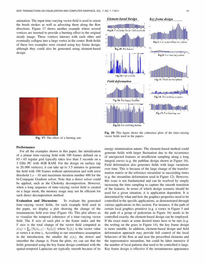
animation. The input time-varying vector field is used to orientthe brush strokes as well as advecting them along the flowdirections. Figure 17 shows another example where severalvortices are inserted to provide a burning effect to the originalsteady image. These vortices interact with each other andeventually collapse into a large vortex in the center. Both fieldsof these two examples were created using key frame design,although they could also be generated using element-baseddesign.

Fig. 17: The effect of a burning sun.

PerformanceFor all the examples shown in this paper, the initialization

of a planar time-varying field with 100 frames defined on a65×65 regular grid typically takes less than 5 seconds on a3 GHz PC with 4GB RAM. For the design on surface (upto 20,000 vertices), it can take up to 3.5 minutes to generatethe field with 100 frames without optimization and with errorthreshold 1.e−10 and maximum iteration number 400 for thebi-Conjugate Gradient solver. Note that a direct solver couldbe applied, such as the Cholesky decomposition. However,when a long sequence of time-varying vector field is createdon a large mesh, the memory usage may not be efficient forsuch direct decomposition method.

Evaluation and Discussion: To evaluate the generatedtime-varying vector fields, for each example field used inthe paper, we display a plot showing the change of theinstantaneous field over time (Figure 18). This plot allows usto visualize the temporal coherence of a time-varying vectorfield. The X axis of each plot is the frame index and theY axis is the total change of the vector field computed asy(xi) = ∑k ||Vk(ti+1)−Vk(ti)|| where Vk(ti) is the vector valueat vertex k at time ti. According to our smoothness assumptionin the introduction, the smaller the y(xi), the slower andsmoother the change is. From the plots, we can see that thefields generated using the key frame design combined with thespatial-temporal Laplacian are typically smooth because of its

Fig. 18: This figure shows the coherence plots of the time-varyingvector fields used in the papers.

energy minimization nature. The element-based method couldgenerate fields with larger fluctuation due to the occurrenceof unexpected features or insufficient sampling along a longintegral curves (e.g. the pathline design shown in Figure 16).Field deformation also generates fields with large variationsover time. This is because of the large change of the transfor-mation matrix or the reference streamline in succeeding times(e.g. the streamline deformation used in Figure 12). However,this issue is not fundamental and can be resolved by simplyincreasing the time sampling to capture the smooth transitionof the features. In terms of which design scenario should beused for a given situation, it is application dependent. It isdetermined by what and how the graphics properties need to becontrolled in the specific applications, as demonstrated throughvarious applications in this section. For instance, if the path ofcertain local graphics primitive (e.g. a vortex in Figure 5 andthe path of a group of pedestrian in Figure 16) needs to becontrolled exactly, the element-based design can be employed.If the exact states at some desired times have to be met (e.g.the writing on the grass in Figure 14), the key frame designis more suitable. In addition, element-based design and fielddeformation approach may provide full control of the localbehaviors of the flow at and near the prescribed elements andthe representative streamline, but could be labor intensive ifthe number of local patterns that need to be controlled is large.Key frame design is effective if the instantaneous appearance


is the main goal and only a few instantaneous fields at thedesired times are required to meet, but is lack of the control ofthe rest of the field. An ideal solution will be the combinationof these different approaches to devise a more flexible andthorough design framework. We plan to investigate this in thefuture work.

10 CONCLUSION AND FUTURE WORKThis paper addresses the problem of the design of time-varying vector field on 2D domains. We have identified aset of design requirements as well as provided a system anda user interface for the design of 2D time-varying vectorfields. A number of design primitives are then discussed basedon the requirements of two different types of vector fields,i.e., orientation and advection fields, for different purposesin computer graphics. Efficient algorithms are introduced togenerate time-varying vector fields from the user specifieddesign elements. A number of editing operations with certaintopological guarantees are introduced to enable the adjustmentof the initial fields. To our knowledge, the presented designframework is the first of its kind for general time-varyingvector field design with bifurcation control. This work opensa new range of the field design topics which can be extendedto the higher order time-varying tensor field design [27]. Forinstance, the same framework can be easily modified to handlethe design of time-varying tensor fields by extending the time-varying singular elements to the elements for degenerate pointsin the element-based design or solving a tensor-based spatial-temporal Laplacian in the key frame design.

There are a number of future research directions. First, thepresent generation techniques do not guarantee the desiredtopology over time, especially for key frame design. Only thetopology at the key frame fields are defined. More comprehen-sive control of topology in between key frame fields is needed.Second, the bifurcation design is an important component intime-varying vector field design as shown in the paper. Moreflexible and sophisticated design technique for bifurcationsare desired. We also wish to extend our system to handlemore types of bifurcations that may involve more sophisticatedobjects such as periodic orbits and separation and attachmentlines. Third, we plan to explore other flow descriptors in-cluding streaklines, timelines [7], and Lagrangian coherentstructures [12]. Fourth, comprehensive combinations of theproposed design functionality, such as combined design withsimulation, should be studied to support more complex designtasks in the future. Finally, extending the design techniques for2D fields to 3D domain will be challenging yet more beneficialfor computer graphics.

ACKNOWLEDGMENTSWe would like to thank Dr. Konstantin Mischaikow for thevaluable discussion on the topology and dynamics of vectorfields, which initiated this work. We also thank Dr. Markvan Langeveld for the valuable discussion on potential ap-plications. This work was supported by NSF IIS-0546881,CCF-0830808 awards. Guoning Chen was partially supportedby King Abdullah University of Science and Technology(KAUST) Award No. KUS-C1-016-04 and DOE VACET.

REFERENCES

[1] P. Alliez, D. Cohen-Steiner, O. Devillers, B. Levy, and M. Desbrun.Anisotropic polygonal remeshing. ACM Transactions on Graphics,22(3):485–493, 2003.

[2] A. W. Bargteil, F. Sin, J. E. Michaels, T. G. Goktekin, and J. F. O’Brien.A texture synthesis method for liquid animations. In Proceedings ofthe ACM SIGGRAPH/Eurographics Symposium on Computer Animation,pages 345–351, Sept 2006.

[3] G. Chen, K. Mischaikow, R. S. Laramee, P. Pilarczyk, and E. Zhang.Vector field editing and periodic orbit extraction using morse decom-position. IEEE Transactions on Visualization and Computer Graphics,13(4):769–785, 2007.

[4] S. Chenney. Flow tiles. In SCA ’04: Proceedings of the 2004 ACMSIGGRAPH/Eurographics symposium on Computer animation, pages233–242. Eurographics Association, 2004.

[5] Y.-Y. Chuang, D. B. Goldman, K. C. Zheng, B. Curless, D. H. Salesin,and R. Szeliski. Animating pictures with stochastic motion textures.ACM Transactions on Graphics, 24(3):853–860, 2005.

[6] K. Crane, M. Desbrun, and P. Schroder. Trivial connections on discretesurfaces. Computer Graphics Forum (SGP), 29(5):1525–1533, 2010.

[7] T. Faber. Fluid Dynamics for Physicists. Cambridge University Press,1995.

[8] M. Fisher, P. Schroder, M. Desbrun, and H. Hoppe. Design of tangentvector fields. ACM Transactions on Graphics, 26(3):56:1–56:9, 2007.

[9] M. S. Floater. Mean value coordinates. Comput. Aided Geom. Des.,20(1):19–27, 2003.

[10] H. Fu, Y. Wei, C.-L. Tai, and L. Quan. Sketching hairstyles. In SBIM’07: Proceedings of the 4th Eurographics workshop on Sketch-basedinterfaces and modeling, pages 31–36. ACM, 2007.

[11] J. Hale and H. Kocak. Dynamics and Bifurcations. New York: Springer-Verlag, 1991.

[12] G. Haller. Finding finite-time invariant manifolds in two-dimensionalvelocity fields. Chaos, 10(1):99–108, 2000.

[13] J. Han, K. Zhou, L.-Y. Wei, M. Gong, H. Bao, X. Zhang, and B. Guo.Fast example-based surface texture synthesis via discrete optimization.Vis. Comput., 22(9):918–925, 2006.

[14] J. Hays and I. Essa. Image and video based painterly animation. InNPAR ’04: Proceedings of the 3rd international symposium on Non-photorealistic animation and rendering, pages 113–120, New York, NY,USA, 2004. ACM.

[15] J. L. Helman and L. Hesselink. Representation and Display of VectorField Topology in Fluid Flow Data Sets. IEEE Computer, 22(8):27–36,August 1989.

[16] A. Hertzmann. Painterly rendering with curved brush strokes of multiplesizes. In SIGGRAPH ’98: Proceedings of the 25th annual conferenceon Computer graphics and interactive techniques, pages 453–460, NewYork, NY, USA, 1998. ACM.

[17] A. Hertzmann and K. Perlin. Painterly rendering for video and inter-action. In NPAR ’00: Proceedings of the 1st international symposiumon Non-photorealistic animation and rendering, pages 7–12, New York,NY, USA, 2000. ACM.

[18] M. Kagaya, W. Brendel, Q. Deng, T. Kesterson, S. Todorovic, P. J. Neill,and E. Zhang. Video painting with space-time-varying style parameters.IEEE Transactions on Visualization and Computer Graphics, 17(1):74–87, 2011.

[19] V. Kwatra, D. Adalsteinsson, T. Kim, N. Kwatra, M. Carlson, andM. Lin. Texturing fluids. IEEE Transactions on Visualization andComputer Graphics, 13(5):939–952, 2007.

[20] V. Kwatra, I. Essa, A. Bobick, and N. Kwatra. Texture optimization forexample-based synthesis. ACM Transactions on Graphics, SIGGRAPH2005, pages 795–802, August 2005.

[21] Y.-K. Lai, M. Jin, X. Xie, Y. He, J. Palacios, E. Zhang, S.-M. Hu,and X. Gu. Metric-driven rosy field design and remeshing. IEEETransactions on Visualization and Computer Graphics, 16(1):95–108,2010.

[22] R. S. Laramee, B. Jobard, and H. Hauser. Image space based visualiza-tion of unsteady flow on surfaces. In Proceedings IEEE Visualization’03, pages 131–138. IEEE Computer Society, October 2003.

[23] S. Lefebvre and H. Hoppe. Appearance-space texture synthesis. ACMTrans. Graph., 25(3):541–548, 2006.

[24] C. Ma, L.-Y. Wei, B. Guo, and K. Zhou. Motion field texture synthesis.ACM Transactions on Graphics, (Proceedings SIGGRAPH Asia 2009),28(5):110:1–110:8, 2009.

[25] O. Mallo, R. Peikert, C. Sigg, and F. Sadlo. Illuminated lines revisited.In Proceeding of IEEE Visualization 2005, pages 19–26, Los Alamitos,CA, USA, 2005. IEEE Computer Society.


[26] F. Neyret. Advected textures. In Proceedings of the 2003 ACMSIGGRAPH/Eurographics symposium on Computer animation, SCA ’03,pages 147–153, Aire-la-Ville, Switzerland, Switzerland, 2003. Euro-graphics Association.

[27] J. Palacios and E. Zhang. Rotational symmetry field design on surfaces.ACM Transactions on Graphics, 26(3):56:1–56:10, 2007.

[28] R. Parent. Computer Animation, Second Edition: Algorithms andTechniques. Morgan Kaufmann Publishers Inc., San Francisco, CA,USA, 2007.

[29] S. Patil, J. van den Berg, S. Curtis, M. C. Lin, and D. Manocha.Directing crowd simulations using navigation fields. IEEE Transactionson Visualization and Computer Graphics, 17:244–254, February 2011.

[30] F. Pighin, J. M. Cohen, and M. Shah. Modeling and editing flowsusing advected radial basis functions. In SCA ’04: Proceedings ofthe 2004 ACM SIGGRAPH/Eurographics symposium on Computer an-imation, pages 223–232, Aire-la-Ville, Switzerland, Switzerland, 2004.Eurographics Association.

[31] E. Praun, F. Adam, and H. Hugues. Lapped textures. In Proceedings ofACM SIGGRAPH 2000, pages 465–470, July 2000.

[32] W. H. Press, S. A. Teukolsky, W. T. Vetterling, and B. P. Flannery.Numerical Recipes in C: The Art of Scientific Computing. New York,NY, USA: Cambridge University Press, 1992.

[33] N. Ray, W. C. Li, B. Lvy, and A. S. an d Pierre Alliez. Periodic globalparameterization. ACM Transactions on Graphics, 25(4):1460–1485,2006.

[34] N. Ray, B. Vallet, W.-C. Li, and B. Levy. N-symmetry direction fielddesign. ACM Transactions on Graphics, 27(2):10:1–10:13, 2008.

[35] J. Stam. Stable fluids. In Proceedings of the 26th annual conference onComputer graphics and interactive techniques, SIGGRAPH ’99, pages121–128. ACM Press/Addison-Wesley Publishing Co., 1999.

[36] J. Stam. Flows on surfaces of arbitrary topology. volume 22, pages724–731, New York, NY, USA, July 2003. ACM.

[37] H. Theisel. Designing 2d vector fields of arbitrary topology. ComputerGraphics Forum (Proceedings Eurographics 2002), 21(3):595–604, July2002.

[38] H. Theisel, T. Weinkauf, H.-C. Hege, and H.-P. Seidel. Topologicalmethods for 2d time-dependent vector fields based on stream lines andpath lines. IEEE Transactions on Visualization and Computer Graphics,11(4):383–394, 2005.

[39] A. Treuille, S. Cooper, and Z. Popovic. Continuum crowds. ACMTransactions on Graphics, 25(3):1160–1168, 2006.

[40] X. Tricoche, G. Scheuermann, and H. Hagen. Topology-based visualiza-tion of time-dependent 2d vector fields. In Data Visualization 2001 (JointEurographics-IEEE TCVG Symposium on Visualization Proceedings),pages 117–126, 2001.

[41] G. Turk. Texture synthesis on surfaces. Computer Graphics Proceedings,Annual Conference Series (SIGGRAPH 2001), pages 347–354, 2001.

[42] G. Turk and J. F. O’brien. Modelling with implicit surfaces thatinterpolate. ACM Transactions on Graphics, 21(4):855–873, October2002.

[43] J. van Wijk. Image based flow visualization for curved surfaces. InProceedings IEEE Visualization ’03, pages 123–130. IEEE ComputerSociety, 2003.

[44] J. J. van Wijk. Image based flow visualization. In SIGGRAPH ’02:Proceedings of the 29th annual conference on Computer graphics andinteractive techniques, pages 745–754. ACM, 2002.

[45] W. von Funck, H. Theisel, and H.-P. Seidel. Vector field based shapedeformations. ACM Transactions on Graphics, 25(3):1118–1125, 2006.

[46] L. Y. Wei and M. Levoy. Texture synthesis over arbitrary manifoldsurfaces. Computer Graphics Proceedings, Annual Conference Series(SIGGRAPH 2001), pages 355–360, 2001.

[47] J. Wejchert and D. Haumann. Animation aerodynamics. In Proceedingsof the 18th annual conference on Computer graphics and interactivetechniques, SIGGRAPH ’91, pages 19–22. ACM, 1991.

[48] K. Xu, D. Cohne-Or, T. Ju, L. Liu, H. Zhang, S. Zhou, and Y. Xiong.Feature-aligned shape texturing. ACM Transactions on Graphics (SIG-GRAPH Asia 2009), 28(5):108:1–108:7, 2009.

[49] K. Xu, H. Zhang, D. Cohen-Or, and Y. Xiong. Dynamic harmonic fieldsfor surface processing. Computers and Graphics (Special Issue of ShapeModeling International), 33:391–398, 2009.

[50] L. Xu, J. Chen, and J. Jia. A segmentation based variational model foraccurate optical flow estimation. pages 671–684, 2008.

[51] E. Zhang, K. Mischaikow, and G. Turk. Vector field design on surfaces.ACM Transactions on Graphics, 25(4):1294–1326, 2006.

Guoning Chen received a bachelors degree in1999 from Xi’an Jiaotong University, China and amasters degree in 2002 from Guangxi University,China. In 2009, he received a PhD degree incomputer science from Oregon State University.His research interests include scientific visual-ization, computational topology, and computergraphics. Currently, he is a post-doctoral re-search associate in Scientific Computing andImaging (SCI) Institute at the University of Utah.He is a member of the IEEE.

Vivek Kwatra Vivek Kwatra received the BTechdegree in computer science and engineeringfrom the Indian Institute of Technology (IIT)Delhi, India, in 1999 and the MS and PhD de-grees in computer science from the Georgia In-stitute of Technology in 2004 and 2005, respec-tively. He was a postdoctoral researcher in theComputer Science Department at the Universityof North Carolina, Chapel Hill, from 2005 to2007. He is currently working at Google as aresearch scientist.

Li-Yi Wei is a researcher with Microsoft Re-search and an associate professor at The Uni-versity of Hong Kong. Before that he has beenarchitecting graphics chips with NVIDIA until2005. He obtained Ph.D. from Stanford in 2001.He likes computer graphics because it covers avariety of subjects in art, science, and engineer-ing. He is also interested in parallel computing,hardware architecture, human computer interac-tion, or whatever subjects that his collaboratorsforce him to learn.

Charles D. Hansen received a BS in computerscience from Memphis State University in 1981and a PhD in computer science from the Univer-sity of Utah in 1987. He is a professor of com-puter science at the University of Utah an asso-ciate director of the SCI Institute. From 1989 to1997, he was a Technical Staff Member in theAdvanced Computing Laboratory (ACL) locatedat Los Alamos National Laboratory, where heformed and directed the visualization efforts inthe ACL. He was a Bourse de Chateaubriand

PostDoc Fellow at INRIA, Rocquencourt France, in 1987 and 1988.His research interests include large-scale scientific visualization andcomputer graphics.

Eugene Zhang received the PhD degree incomputer science in 2004 from Georgia Insti-tute of Technology. He is currently an associateprofessor at Oregon State University, where heis a member of the School of Electrical Engi-neering and Computer Science. His researchinterests include computer graphics, scientificvisualization, geometric modeling, and computa-tional topology. He received an National ScienceFoundation (NSF) CAREER award in 2006. Heis a member of the IEEE and a senior member

of ACM.

ieee transactions on visualization and computer …chengu/publications/timedep_vfdsurf.pdf · ieee...

Documents