identification of key determinants of geo-mechanical

13th International Conference on Applications of Statistics and Probability in Civil Engineering, ICASP13 Seoul, South Korea, May 26-30, 2019

1

Identification of key determinants of geo-mechanical behavior of an instrumented buried pipe

Humberto Yáñez-Godoy Associate Professor, I2M, University of Bordeaux, France

Sidi Mohammed Elachachi Professor, I2M, University of Bordeaux, France

Olivier Chesneau Head of Asset Management Department, SEDIF (Syndicat des eaux d’Ile de France), Paris, France

Cédric Feliers Head of R&D Department, VEDIF (Veolia Eau d’Ile de France), Paris, France

ABSTRACT: The instrumentation of extended buried structures provides access to a better understanding of the mechanisms that control the behavior of these structures and those that can affect their durability and lead to their deterioration. In this paper, the follow-up of a new installed and instrumented buried reinforced concrete pressurized pipe is presented. A sensor-enabled geotextile is used in this project to measure ground strains along the new pipeline. The monitoring data let to identify some key determinants as the spatial structure of soil to assess the behavior of the structure under certain loading conditions. A case study illustrates a bidimensional geo-mechanical finite element model of a buried pipeline. A spatial variability approach coupled to the mechanical model allows assessing the risk a pipe presents during operational service at a given time with respect to predefined limit state performance criteria.

The refurbishment of water pipelines is required as a result of the natural process of aging which leads to a gradual lowering of their original performance level. Asset management of these structures aims at maintaining the infrastructure facility in satisfactory conditions in relation to technological, environmental, societal and/or socio-economic issues. Asset management includes the process of acquiring information (and its storage in the form of databases), the assessment of the performance of the infrastructure facility (by defining indicators/criteria, Liu et al. (2012)) and the refurbishment of elements or subsystems considered defective or as being at risk. The follow-up of new pipes coupled to an instrumentation on the site improve the data basis of numerical models used to understand for example the physical mechanisms underlying

degradation of these structures (Deo et al. (2018)) or the earth pressures on the pipes during the construction phase (Zhou et al. (2017)). Monitoring data can contribute to identify some key determinants to assess the behavior of buried pipelines under certain loading conditions. The main interest is to study, at the local scale (that is a single element of the real-estate patrimony), the behavior of buried pipelines from the precisely point of view of the geo-mechanics. A numerical model which represents in a proper way the instrumented pipe should be built to study the buried pipe loaded in different situations. The numerical models will be enriched by the data obtained from monitoring and can then be used to asses better a whole range of loading conditions. Asset managers can then have access to these decision-making tools to optimize the resource flows at the global scale (the property assets). An


2

instrumented buried pipeline presented in this paper illustrates the individual steps to provide a decision-making tool.

1. STUDY AREA The replaced water pipeline segment is 90 m length and 800 mm inside diameter, it is located in Saint-Denis, a commune in the northern suburbs of Paris, France. The mean depth at which the pipe is buried is 2.3 m. The main axial plane of the pipeline is adjacent to an important traffic lane.

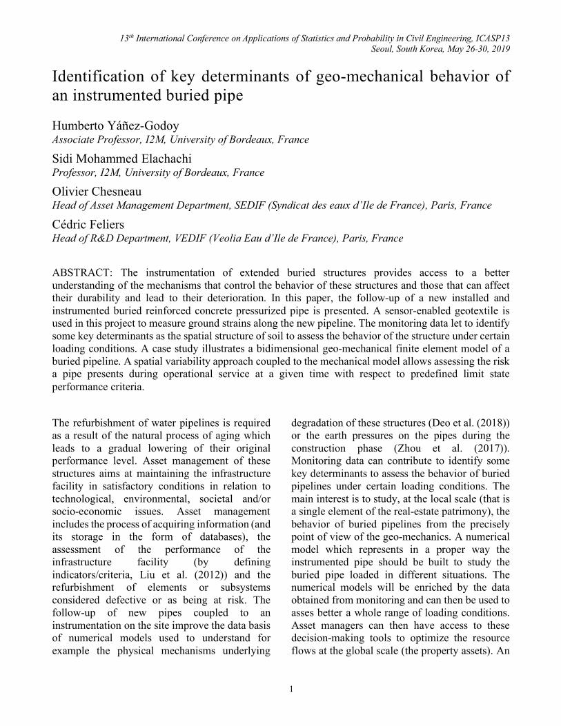
1.1. Concrete pressurized pipe The concrete pressurized pipe is a steel cylinder embedded in a concrete core. These concrete pipes are also known as bonna pipes. Figure 1 shows this kind of pipe and its main components such as those built in North America (USA) or in Europe (France).

Figure 1: Diagram of a bonna pipe.

2. MEASURES This section presents the technology used to instrument the system soil-pipe and its implementation on the study area. Data collected from one year of measurements are also analyzed.

2.1. Sensor-enabled geotextile The measurement technology used is the Brillouin distributed optical fiber sensor (Galindez-Jamioy C.A. and López-Higuera J.M. (2012)). Brillouin scattering of light is employed to measure the strain in the optical fibers. The sensor-enabled geotextile used in this project to measure ground strains is composed by two strips of geotextile. Four optical fiber cables are embedded in each

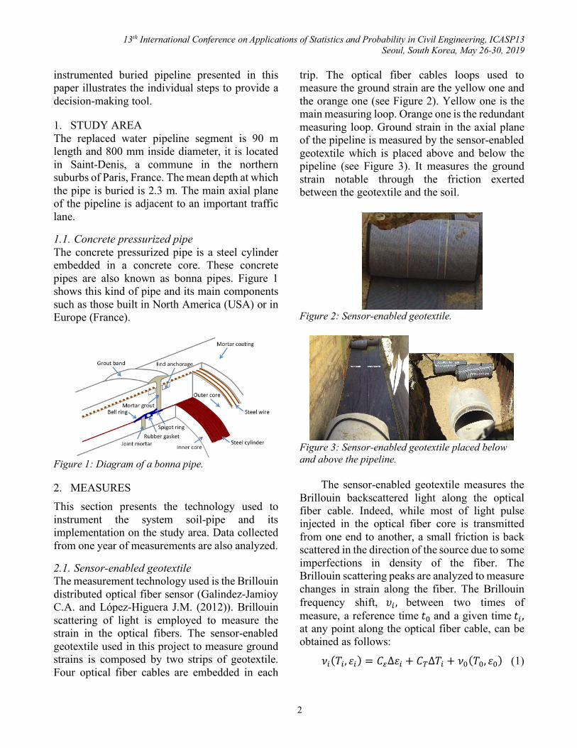
trip. The optical fiber cables loops used to measure the ground strain are the yellow one and the orange one (see Figure 2). Yellow one is the main measuring loop. Orange one is the redundant measuring loop. Ground strain in the axial plane of the pipeline is measured by the sensor-enabled geotextile which is placed above and below the pipeline (see Figure 3). It measures the ground strain notable through the friction exerted between the geotextile and the soil.

Figure 2: Sensor-enabled geotextile.

Figure 3: Sensor-enabled geotextile placed below and above the pipeline.

The sensor-enabled geotextile measures the

Brillouin backscattered light along the optical fiber cable. Indeed, while most of light pulse injected in the optical fiber core is transmitted from one end to another, a small friction is back scattered in the direction of the source due to some imperfections in density of the fiber. The Brillouin scattering peaks are analyzed to measure changes in strain along the fiber. The Brillouin frequency shift, 𝜐", between two times of measure, a reference time 𝑡% and a given time 𝑡", at any point along the optical fiber cable, can be obtained as follows:

𝜈"(𝑇", 𝜀") = 𝐶-Δ𝜀" + 𝐶0Δ𝑇" + 𝜈%(𝑇%, 𝜀%) (1)


3

where 𝜐" depends on both the applied strain variation, Δ𝜀", and the temperature variation, Δ𝑇"; 𝜐% is the Brillouin frequency at reference time, 𝑡%; the coefficients 𝐶- = 0.02MHz/𝜇𝜀 and 𝐶0 = 1 MHz/°C are respectively the constant strain and temperature coefficients. Temperature can also be obtained by the sensor (black and blue optical fiber cables showed in Figure 2) but this parameter is not measured because the depth of the geotextile implanted in the soil ensures a steady temperature in a range ±5°. The strain variation at a given time 𝑡" is as follows:

Δ𝜀" = Δ𝑣"/𝐶- (2)

where Δ𝑣" is the Brillouin frequency variation at a given time 𝑡".

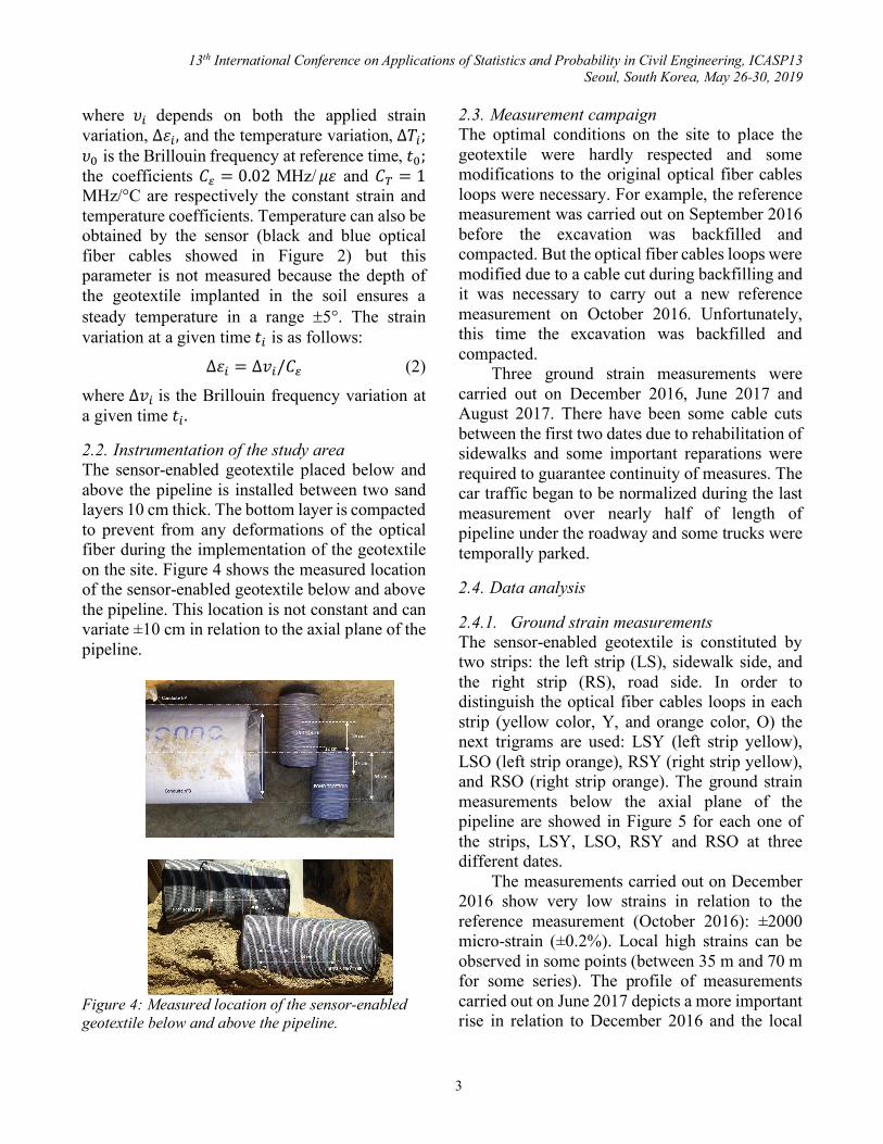
2.2. Instrumentation of the study area The sensor-enabled geotextile placed below and above the pipeline is installed between two sand layers 10 cm thick. The bottom layer is compacted to prevent from any deformations of the optical fiber during the implementation of the geotextile on the site. Figure 4 shows the measured location of the sensor-enabled geotextile below and above the pipeline. This location is not constant and can variate ±10 cm in relation to the axial plane of the pipeline.

Figure 4: Measured location of the sensor-enabled geotextile below and above the pipeline.

2.3. Measurement campaign The optimal conditions on the site to place the geotextile were hardly respected and some modifications to the original optical fiber cables loops were necessary. For example, the reference measurement was carried out on September 2016 before the excavation was backfilled and compacted. But the optical fiber cables loops were modified due to a cable cut during backfilling and it was necessary to carry out a new reference measurement on October 2016. Unfortunately, this time the excavation was backfilled and compacted.

Three ground strain measurements were carried out on December 2016, June 2017 and August 2017. There have been some cable cuts between the first two dates due to rehabilitation of sidewalks and some important reparations were required to guarantee continuity of measures. The car traffic began to be normalized during the last measurement over nearly half of length of pipeline under the roadway and some trucks were temporally parked.

2.4. Data analysis

2.4.1. Ground strain measurements The sensor-enabled geotextile is constituted by two strips: the left strip (LS), sidewalk side, and the right strip (RS), road side. In order to distinguish the optical fiber cables loops in each strip (yellow color, Y, and orange color, O) the next trigrams are used: LSY (left strip yellow), LSO (left strip orange), RSY (right strip yellow), and RSO (right strip orange). The ground strain measurements below the axial plane of the pipeline are showed in Figure 5 for each one of the strips, LSY, LSO, RSY and RSO at three different dates.

The measurements carried out on December 2016 show very low strains in relation to the reference measurement (October 2016): ±2000 micro-strain (±0.2%). Local high strains can be observed in some points (between 35 m and 70 m for some series). The profile of measurements carried out on June 2017 depicts a more important rise in relation to December 2016 and the local


4

strains are even more important: ±10000 micro-strain (±1%) for some profiles. The variation of strain between the profiles August 2017 and June 2017 is very low that allow us to suppose a stabilization of differential settlements along the pipeline.

(a)

(b)

(c)

(d)

Figure 5: Ground strain measurements below the pipeline at three different dates: (a) right strip yellow RSY, (b) right strip orange RSO, (c) left strip yellow LSY, and (d) left strip orange LSO.

2.4.2. Spatial series analysis: empirical semivariogram

Each profile of ground strain measurements presented in Figure 5 is considered as a spatial series. The analysis of these spatial series is performed in this section by computing an empirical semivariogram (Iris J.-M. (1986)). This function let to describe the degree of spatial dependence of each series. For the measured series, the covariance between points is computed and let to analyse how acquired information deteriorates on one point when moving away from this one. The semivariogram of a variable Z for a lag h between two adjacent points (x) and (x + h) is computed as follows:

γ(ℎ) = <=× 𝐸 @AZ(𝑥 + ℎ) − Z(𝑥)E

=F (3)

where 𝐸[(. )=] is the expectation for the squared increment of the values between locations (x) and (x + h).

As observed in Figure 5, the series on June 2017 become more stable. The semivariogram is therefore computed, in Figure 6, for the series LSY, LSO, RSY and RSO for June 2017 only.


5

Figure 6: Empirical semivariogram of ground strain measurements below the pipeline for the series LSY, LSO, RSY and RSO for June 2017.

Figure 6 shows particularly two sills starting

at different ranges for all the series. A first sill starts in a range about between 2 m and 5 m. A second sill starts in a range about between 10.5 m and 29 m. The two values of the first range represent about 30% and 80% of the length of the concrete pipe (6 m). Comparatively, a semivariogram was computed from penetrometer measures in Breysse et al. (2002) for a buried concrete sewage network; the range value obtained was 3 m. This value falls within the first interval range (2 m and 5 m).

2.4.3. Spatial series analysis: computed mean semivariogram

In this section, the mean semivariogram is computed from parameters observed in Figure 6. Table 1 shows a summary of all the parameters observed in the empirical semivariograms. The range value to be retained is the mean of the values observed in the first range, i.e. 3.3 m. The value of the variance (Y-axis in Figure 6), to be retained is the mean of the values observed in the two sills, i.e. 1.41×106.

Table 1: Values of first range and sills observed for semivariogram of each series.

Series First range (m)

First sill (variance)

Second sill (variance)

RSY 5 8.134×105 2.276×106 RSO 3.6 6.865×105 1.098×106

LSY 2.2 6.235×105 1.380×106 LSO 2.6 9.582×105 3.445×106 Mean value

retained 3.3 1.41×106

Firstly, to compute the mean semivariogram,

a random field, 𝜀I(𝑥) representing the spatial ground strain measurements below the pipeline (X-axis in Figure 5) is generated by using the fast Fourier transform method (Yang J.-N. (1972)). A normal inverse cumulative distribution function, F-1, is considered as follows:

𝜀I(𝑥) = 𝐹K<A𝐹(𝑀(𝑥)|𝜇, 𝜎)E (4)

where 𝐹(𝑀(𝑥)|𝜇, 𝜎) is the cumulative distribution function of a zero-mean, µ, normal random process, 𝑀(𝑥) , with 𝜎 = √1.41 × 106 . The generated 𝑀(𝑥) process associates a single exponential correlation function 𝜌(𝜏) defined as:

𝜌(𝜏T) = 𝑒𝑥𝑝 W−2 |XY|ZY[ (5)

where 𝜏T = 0.2 m and 𝛿T = 3.3 m are the distance between data points in the random field and the correlation length of 𝜀I(𝑥) in the soil length direction (X-axis in Figure 5), respectively.

Second, by using Monte-Carlo simulations, several random fields are generated for 𝜀I(𝑥). For example, Figure 7 shows ground strain measurements for the LSO series for June 2017 and 100 simulations generated for 𝜀I(𝑥).

Figure 7: Ground strain measurements for series LSO (in red dotted line) and computed random field of ground strain (100 simulations in black dotted line) below the pipeline for June 2017.


6

Third, for each simulated random field, a computed semivariogram is obtained by using Eq. (3). Figure 8 shows the computed mean semivariogram, for 104 simulations, of ground strain measurements below the pipeline for June 2017. Mean range computed is 4.8 m which corresponds to a variance value equals to 1.33×106 (95% of the mean computed sill).

Figure 8: Computed mean semivariogram (104 simulations) of ground strain measurements below the pipeline for June 2017.

3. CASE STUDY The case study is a mechanical model constituted by a concrete pipeline buried in a soil. It represents about half of the length of the pipeline in the study area. The mechanical model was developed within the CAST3M finite element computer code (http://www-cast3m.cea.fr).

3.1. Mechanical modelling The characteristics of both the concrete pipeline (48 m length), constituted by 8 individual pipe segments (each of 6 m length), and the surrounding ground are given in Table 2. Finite element mesh of the system soil-pipe is presented in Figure 9.

Figure 9: Finite element mesh used for the case study Y-axis ↑→ X-axis.

Table 2: Concrete pipeline and surrounding soil characteristics.

Geometrical concrete pipe

characteristics

Surrounding soil characteristics Loading

Total length L = 48 m Inside diameter Dext = 0.8 m Thickness ep = 0.074 m Pipe length lp = 6 m Young’s modulus of bonna pipe Ec = 36 GPa (short-term strength)

Poisson coefficient of bonna pipe vc = 0.2 Young’s modulus of steel joint Ej = 210 GPa Poisson coefficient of steel joint vj = 0.3

Compacted layer Depth Hs1 = 1.5 m Young’s modulus Es1 = 50 MPa Friction angle j’1 = 25° Poisson coefficient νs1 = 0.3 Cohesion c1 = 1 kPa Dry unit weight g1 = 20 kN/m3

Natural ground Depth Hs2 = 4 m Young’s modulus Es2 = 6 MPa Friction angle j’2 = 25° Poisson coefficient νs2 = 0.35 Cohesion c2 = 1 kPa Dry unit weight g2 = 20 kN/m3

Service pressure

Wp = 1200 kPa Working load:

q = 62 kPa

A combination of self-weight (pipe, soil,

water), service pressure (1200 kPa) and working load (62 kPa on the compacted layer above the two central pipe segments) is considered. The depth dimension of the natural ground corresponds to the dimension normally used in the literature, above 5 times the external diameter of the pipe (e.g. Rubio et al. (2007)). The pipe is modelled with planar elements and is assumed to act in an isotropic and linearly elastic manner. The mechanical model employs the Mohr-Coulomb model to describe the soil behavior. The interfaces between the soil and the structure and between two individual pipe segments are modelled using joint elements. These are numerical interfaces with small thickness values, very close or equal to

Natural ground

PipelineCompacted layer

q


7

zero. None horizontal loading is considered in the pipe, that let us to assume that pipe-soil system behaves as a rigid element without not influence of numerical interfaces (soil or pipe joint stiffness).

3.2. Soil spatial variability A sensitivity analysis would be necessary to identify the most sensitive parameters for simplify probabilistic computations. In this case study, the natural spatial randomness of the soil is considered by looking at the Young’s modulus Es2 (natural ground) as a sensitive parameter. An unidimensional random field is considered to create a model of the soil spatial variability. The other parameters (geotechnical and geometrical concrete pipe parameters, external and internal loading) are considered as deterministic.

The beta distribution is adopted to generate simulations of the random field of Young’s modulus Es2, along the soil length direction X, according to Figure 9. That avoids to generate negative values for this parameter. Mean value is 𝜇 _̂` = 6 MPa. A coefficient of variation, COV (10%, 20% and 30%), is applied to 𝜇 _̂`, standard deviation is then 𝜎 _̂` = 𝐶𝑂𝑉 × 𝜇 _̂` . Young’s modulus Es2 parameter is bounded between two extreme values: 𝐸c=d"e = 2 MPa and 𝐸c=dfI =10 MPa. The beta probability distribution is written, as follows (Yáñez-Godoy H. et al. (2017)):

𝐸c= = A𝐸c=dfI − 𝐸c=d"eE ∙ 𝑍 + 𝐸c=d"e (6)

where Z is a beta random variable with values in [0,1] .The beta inverse cumulative distribution function, F-1, is obtained as follows:

𝐸c=(𝑥) = 𝐹K<(𝐹(𝑀(𝑥)|𝜇, 𝜎)|𝑎, 𝑏) (7)

where 𝑎, 𝑏 are the parameters of the beta random variable Z in Eq. (6) (Yáñez-Godoy H. et al. (2017)), 𝐹(𝑀(𝑥)|𝜇, 𝜎) is the cumulative distribution function of a zero-mean, µ, normal random process, 𝑀(𝑥) , with 𝜎 = 𝜎 _̂` . The random field is generated by using the fast Fourier transform method. The generated 𝑀(𝑥) process associates a single exponential correlation

function 𝜌(𝜏) as defined in Eq. (5). Here 𝜏T =0.2 m is the distance between data points in the random field and 𝛿T = 4.8 m is the computed value obtained in section 2.4.3 for the correlation length of 𝐸c= in the soil length direction X.

3.3. Propagation of uncertainty The propagation of uncertainty via the finite element model developed within the CAST3M finite element computer code is performed by direct Monte-Carlo numerical simulation method using the MATLAB Statistics Toolbox. Soil spatial variability is modelled by several realizations of a beta random field of Young’s modulus in natural ground, which are generated using the spectral approach presented in section 3.2, and are then entered into the finite element model (Figure 9). A post-processing of results let to assess the structural integrity of the pipe.

3.4. Assessing of structural integrity The dysfunction leading to an exceedance of a limit state considered here is the structural integrity. This is expressed in terms of bending stresses with a limit state function that assesses the cracking state for a concrete pipe as:

𝑔m = 𝜎n − 𝜎o ≤ 0 (8)

where 𝜎n is the yield tensile strength of concrete (mean = 2.2 MPa, standard deviation = 0.1 MPa) and 𝜎o is the maximum bending stress computed with the mechanical model presented in section 3.1. 𝜎n and 𝜎o are considered to follow Lognormal distributions. The Hasofer-Lind reliability index β is defined as (Lemaire M. et al. (2005)):

𝛽 =restuvA<wxyzu

È A<wxyztÈ{ |

}/`~

�revA<wxyzuÈ×A<wxyzt

È|�}/` (9)

where R, S are respectively 𝜎n , 𝜎o and COV is their coefficient of variation. The corresponding probability of failure is 𝑃� = Φ(−𝛽). The target value of β to be reached in Eurocode 1 is equal to 1.5 for the SLS (serviceability limit state) (NF EN 1991-1-1 (2003)). Table 3 shows the values of β in function of the COV of 𝜇 _̂` (10%, 20% and


8

30%) for 1000 simulations. As it can be seen, the longer the dispersion of 𝐸c= (highly heterogeneous soil) the longer its notably effect on reaching early the target value. Table 3: Variation of reliability index β in function of COV of 𝜇 _̂` for 1000 simulations.

β COV of 𝜇 _̂` 5.2 10% 2.5 20% 1.7 30%

4. CONCLUSIONS The complexity to optimize the management of water pipelines requires some strategies to be applied at different scales. Geo-mechanics has been considered in this paper to study, at the local scale, the behavior of buried pipelines. The approach has a double dimension: experimental (monitoring) and numerical (finite element model). Measurement campaign allowed accessing to data not available in current database which are needed to a better understanding of the involved physical mechanisms. The enriched mechanical model illustrated in the case study let to assess the structural integrity of the pipeline. This case study shows the need to take the soil spatial variability into account with knowledge of the spatial continuity of soil properties. These tools can provide experts with decision-making elements for an improved calibration of safety in soil-structure interaction problems when the soil variability is an important parameter. Other key determinants from monitoring will be addressed in future analyses.

5. REFERENCES Breysse D., Elachachi M., Boukhoulda H. (2002).

Modélisation des désordres dans les réseaux enterrés consécutifs à l’hétérogénéité des sols. Journées Nationales de Géotechnique et de Géologie de l’Ingénieur - JNGG2002, Nancy 8-9 octobre.

Deo R.N., Azoor R.M., Zhang C., Kodikara J.K. (2018). Journal of Applied Geophysics, 150(March), 304-313.

Galindez-Jamioy C.A. and López-Higuera J.M. (2012). Brillouin Distributed Fiber Sensors: An Overview and Applications. Journal of Sensors.

Iris J.-M. (1986). Analyse et interprétation de la variabilité spatiale de la densité apparente dans trois matériaux ferrallitiques, Science du Sol, 24(3), 245-256.

Lemaire M., Chateauneuf A., Mitteau J.-C. (2005). Fiabilité des structures : couplage mécano-fiabiliste statique. Paris. Lavoisier.

Liu Z., Kleiner Y., Rajani B., Wang, L., Condit W. (2012). Condition Assessment Technologies for Water Transmission and Distribution Systems. National Risk Management Research Laboratory. United States Environmental Protection Agency, Washington, DC, EPA/600/R-12/017.

NF EN 1991-1-1 (2003). Eurocode 1: Actions on structures. Norme française. Afnor.

Rubio N.P., Roehl D., Romanel C. (2007). A three dimensional contact model for soil-pipe interaction. Journal of Mechanics of Materials and Structures, 2(8), 1501–1513.

Yang J.-N. (1972). Simulation of Random Envelope Processes. Journal of Sound and Vibration, 21(1), 73–85.

Yáñez-Godoy H., Mokeddem A., Elachachi S.M. (2017). Influence of spatial variability of soil friction angle on sheet pile walls’ structural behaviour. Georisk: Assessment and Management of Risks for Engineered Systems and Geohazards, 11(4), 299-314.

Zhou M., Du Y-J, Wang F., Arulrajah A., Horpibulsuk S. (2017). Earth pressures on the trenched HDPE pipes in fine-grained soils during construction phase: Full-scale field trial and finite element modeling. Transportation Geotechnics, 12(September), 56-69.

identification of key determinants of geo-mechanical

Documents