ICES REPORT 14-17

July 2014

Coupled Flow and Geomechanics Modeling for FracturedPoroelastic Reservoirs

by

Gurpreet Singh, Thomas Wick, Mary F. Wheeler, Gergina Pencheva, and Kundan Kumar

The Institute for Computational Engineering and SciencesThe University of Texas at AustinAustin, Texas 78712

Reference: Gurpreet Singh, Thomas Wick, Mary F. Wheeler, Gergina Pencheva, and Kundan Kumar, "CoupledFlow and Geomechanics Modeling for Fractured Poroelastic Reservoirs," ICES REPORT 14-17, The Institutefor Computational Engineering and Sciences, The University of Texas at Austin, July 2014.

Coupled Flow and Geomechanics Modeling for Fractured

Poroelastic Reservoirs

Gurpreet Singh Thomas Wick Mary F. Wheeler Gergina PenchevaKundan Kumar

July 30, 2014

Abstract

The design and evaluation of hydraulic fracture modeling is critical for efficient pro-duction from tight gas and shale plays. The efficiency of fracturing jobs depends on theinteraction between hydraulic (induced) and naturally occurring discrete fractures. Wedescribe a coupled reservoir-fracture flow model which accounts for varying reservoirgeometries and complexities including non-planar fractures. We utilize different flowmodels such as Darcy flow and Reynold’s lubrication equation for fractures and reser-voir to closely capture the physics. Furthermore, the geomechanics effects have beenincluded by considering a multiphase Biot’s model. An accurate modeling of solid de-formations necessitates a better estimation of fluid pressure inside fracture. We modelthe fractures and reservoirs explicitly, which allows us to capture the flow details andimpact of fractures more accurately. The approach presented here is in contrast withexisting averaging approaches such as dual and discrete-dual porosity models where theeffects of fractures are averaged out. A fracture connected to an injection well showssignificant width variations as compared to natural fractures where these changes arenegligible. Furthermore, the capillary pressure contrast between the two is accountedfor by utilizing different capillary pressure curves. We present several numerical tests,including a field scale case study, to illustrate the above features and their impact onrecovery predictions.

Keywords. phase-field; pressurized fractures; iterative coupling algorithm; reservoirsimulation

Introduction

Multiphase flows in fractured reservoirs are of immense importance for energy security.The recovery of hydrocarbons in a reservoir is strongly dependent on the fractures, bothnatural and artificial. To model these processes, it is imperative to have a reliable modelthat captures the effects of these fractures with high accuracy. Moreover, the geometriccomplexities of the fractures require sophisticated numerical approaches. Moreover, thepore pressure from the flow may also cause geomechanical effects. These effects are morepronounced when the fractures are present. The geomechanical effects and multiphaseflows in a fractured porous medium are modeled by coupled nonlinear system of differen-tial equations. Additionally, we need to account properly for reservoir heterogeneities dueto discontinuous rock properties. This manifests in the form of discontinuous changes in

1

absolute permeability, relative permeability and capillary pressure curves. The simulationof this system presents important challenges from both modeling and computational pointsof view. In this work, we perform a quantitative and qualitative study of these effects anddescribe a numerical approach for solving this problem. Our approach offers high accuracyand fidelity in capturing the physics of the problem.

The model consists of two parts: geomechanics and flow equations. The flow equationsin a fractured reservoirs have been a subject of intensive study by several authors. Ourapproach fully resolves the flow by considering separate equations for the fractures andreservoirs which are coupled together. As we shall see later in this section (see Fig 1), thisresolution of fracture flow is important as a crude approximation may lead to unacceptableerrors. The fracture flow model is formulated by reducing a higher dimensional (Rd) modelto a lower dimensional (Rd−1) manifold by averaging procedure. The derivation of thisreduction procedure has been undertaken by Martin et al. (2005) and Frih et al. (2008)for Darcy and Forchheimer flows. The reduction leads to a set of equations defined forboth fractures and reservoirs with fractures acting as interfaces inside the reservoirs. Thepurview of these studies is however limited to single phase flow accounting for permeabilityheterogeneity at the reservoir-fracture interface. We will follow a similar approach here formultiphase flows.

We begin by reviewing some of the work that is relevant to our presented approach.Hoteit and Firoozabadi (2008a) present a good introduction of different finite volume andfinite element based discretizations for such problems. A mixed finite element for multi-phase, reservoir-fracture flow model was proposed by Hoteit and Firoozabadi (2005, 2006)assuming a cross-flow equilibrium across reservoir-fracture interface. This assumption waslater removed (Hoteit and Firoozabadi (2008b)) by considering additional degrees of freedomat the interface. Here, they consider a hybrid mixed method to solve an implicit pressureequation along with a higher order discontinuous Galerkin method with a slope limiter foran explicit saturation update following an IMPES (implicit pressure explicit saturation)scheme. Further, Grillo et al. (2010) discuss density driven flows where fractures are rep-resented as 2 and 3-dimensional manifolds assuming a multi-component, single-phase flowsystem. A finite-volume based numerical discretization is used, with each fracture havingtwo degrees of freedom. Our method is inspired by Hoteit and Firoozabadi (2008a) anduses mixed finite element methods and an IMPES solution scheme. We differ in the usageof a multipoint flux scheme based upon an appropriate choice of finite element spaces andquadrature rule (Ingram et al. (2010),Wheeler and Yotov (2006), Arbogast et al. (1997),Wheeler et al. (2011a)). This approach provides flexibilities in capturing the complex geo-metric features of fractures.

Earlier, a finite-volume based approach was presented by Bastian et al. (2000) andMonteagudo and Firoozabadi (2004) on unstructured grids. The reservoir-fracture interfaceshave only one pressure and saturation degree of freedom and thus jumps in these quantitiescannot be considered, thereby assuming a cross-flow equilibrium. Their model takes intoaccount capillary pressure discontinuity due to rock heterogeneity. However, saturationcalculation at the interface requires inversion of capillary pressure, which may pose problemsif the capillary pressure curve is either identically zero or has a small gradient. Monteagudoand Firoozabadi (2007) address this issue by using two different formulations based uponthreshold values requiring calibration. More recently, a coupled flow in a fractured-reservoir

2

models is considered in Al-Hinai et al. (2013) where different discretization schemes wereutilized inside the fracture (mimetic finite difference) and reservoir (mixed finite element)in the absence of capillary pressure and time invariant fracture permeabilities.

The geomechanical effects in the reservoir are accounted for by considering an elasticdeformable medium. The theoretical groundwork for one-dimensional flow in a deformableporous medium was first developed by Terzaghi (1943). This was later extended to a generaltheory of three-dimensional consolidation for anisotropic and heterogeneous materials byBiot in his subsequent works (Biot (1941a,b, 1955)). For the coupling of multiphase flow andgeomechanics, Settari and Walters (2001) categorize the various schemes as decoupled andexplicit, iterative and fully coupled. An explicit or loose coupling has lower computationaltime with little control on solution accuracy. Further, a time-step size guidance is oftenrequired for the geomechanics solve, which is empirical or heuristic in nature (Dean et al.(2006)). On the other hand, a fully implicit method is both accurate and stable, howeversolving the implicit system of equations results in a complex nonlinear system requiringsuitable linearization schemes and specialized linear solvers for convergence. In this work,we apply an iterative coupling scheme based on fixed stress splitting for which convergenceanalysis has been done in Mikelic and Wheeler (2012); Mikelic et al. (2014); Kim et al.(2012). The analysis shows that the iterative scheme converges geometrically. An iterativecoupling approach combines the advantages of both methods while maintaining numericalsolution accuracy, fast convergence, and ease of implementation in existing legacy flowsimulators.

The poroelastic models rely upon pore-pressure to account for changes in material stress.Accuracy of flow models, especially in capturing sharp pressure changes across a reservoir-fracture interface, plays a pivotal role when poroelastic behavior of reservoir and fracturemechanics comes into play. For a single phase flow, Ganis et al. (2013) presents a coupledflow model fractures in a poroelastic medium. The multipoint flux mixed finite elementmethod (MFMFE) used in this work is defined for general hexahedral grids with non-planaredges. This allows non-planar fracture geometry to be captured. A detailed numericalanalysis for single phase reservoir-fracture flow coupling presented here can be found inGirault et al. (2013).

There are several novelties in this work. We use hexahedral grids with an MFMFEscheme which allows non-planar fractures and an accurate computation of a locally mass-conservative flow profile. Secondly, we resolve the flow equations for both the fractures andreservoir in a coupled manner. This is achieved by assuming a lubrication equation insidethe fractures and multiphase Darcy law for the reservoir. Thirdly, the fixed stress splittingscheme for the geomechanics effects in a reservoir has been extended to include fractureswhere the permeabilities of the fracture are functions of the deformations. Furthermore, ournumerical results have been compared with physical core-scale experiments and benchmarkproblems demonstrating the capabilities of our approach.

We begin with a simplified 2D example to qualitatively outline some of the differencesbetween conventional modeling techniques and the approach presented here. This is followedby a reservoir-fracture flow and geomechanics model formulation with a brief description ofconservation and constitutive equations along with the required closure conditions. We thendiscuss a choice of boundary, interface and initial conditions used to describe the problem.Next in the algorithm and discretization section we briefly outline the spatial and temporal

3

discretization schemes used for flow and mechanics as well as the iterative schemes usedto couple the various systems of equations. Finally, in the results section we present fivenumerical experiments including a comparison with experimental lab results to confirm thevalidity of our model and to further demonstrate the features and long-term predictioncapabilities.

An illustrative example

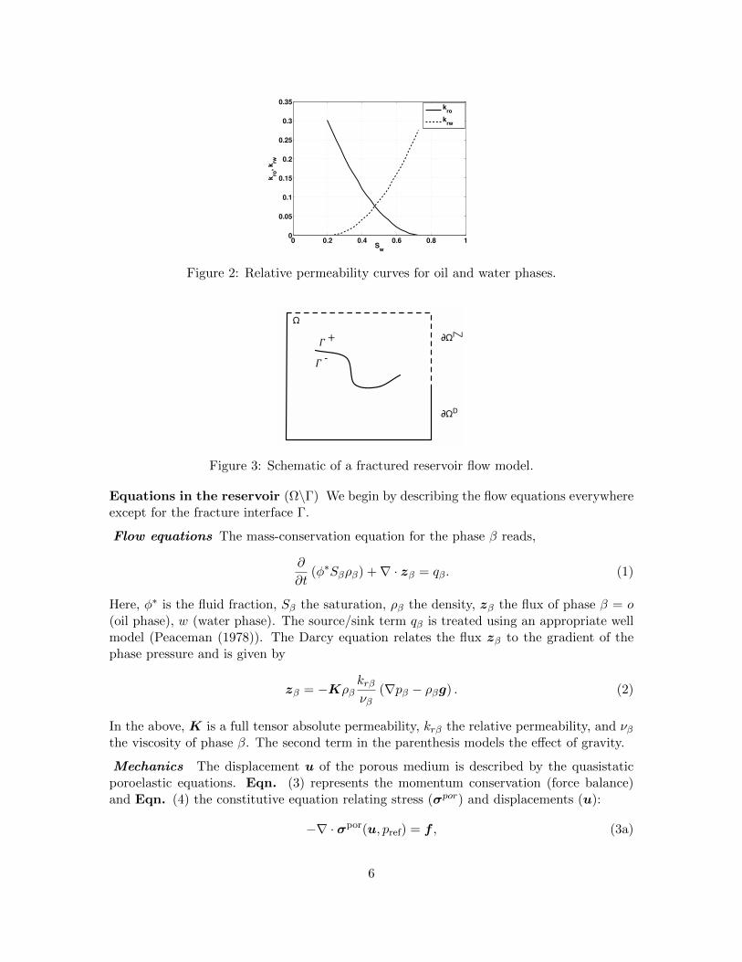
In this section, we motivate this work by emphasizing the need to fully resolve thefracture geometry. The following simplified example underlines the need for a detailedmodeling. This will be achieved by considering and comparing different approaches forfractured reservoir flow modeling. A reservoir domain of size 10 ft×10 ft is considered withbottom-hole pressure specified injection (520 psi) and production (500 psi) wells locatedat diagonally opposite ends. Further, a homogeneous and isotropic reservoir permeabilityof 5 mD and porosity of 0.2 are assumed. Fig. 1 shows saturation profiles for threeapproaches: (1) an average permeability representation (1st row, 1st column), where thedotted red region has been assigned higher average permeability of 5×106 mD assuming thefracture goes through those blocks, (2) a meshed-in representation where the fracture itselfis gridded (1st row, 2nd column) and has a permeability value of 5× 1010 mD, and finally,(3) the interface approach presented in this work (1st row, 3rd column) where the fractureis represented as a lower dimensional surface shown by the red dotted line. The capillarypressure is taken to be identically zero everywhere. The relative permeability curves areshown in Fig. 2.

Note that an actual fracture width of 1 mm is used for the interface approach whencompared to the meshed-in approach where the grid-block width normal to the fracturesurface is 1cm. The saturation profiles at t = 50 and 100 days (2nd and 3rd row in Fig.1) show differences in sweep pattern for the different approaches. The averaging approachmobilizes additional fluid resulting in overestimation of recoveries. The meshed-in approach,although more accurate, poses a few challenges. A mesh refinement is required to capturethe fracture, which may not always be possible. Furthermore, a time-step size restrictiondue to an order of magnitude difference between fracture and reservoir grid block sizes isobserved. A relatively large fracture width (1cm) has been chosen due to time-step sizerestriction imposed by CFL (Courant-Friedrichs-Lewy) condition. The interface approachovercomes these issues while preserving the physics. Fig. 1 (2nd row 3rd column) showsfluid entering fracture at one end and leaving at the other end without mobilizing additionalfluid in between. In the numerical results section, we further elaborate on the merits andthe limitations of the averaging approach. We also show that the orientation and locationof fractures are important parameters in determining the choice of fracture modeling.

Model Formulation

In this section, we provide a brief description of the fractured reservoir flow and ge-omechanics model where fractures are treated as lower dimensional manifolds in (Rd−1)in a reservoir domain Ω ∈ Rd, (d = 2 or 3). The model has two components: two-phaseflow and mechanics. The modeling equations are defined separately in the reservoir and onthe fracture surfaces along with the associated interface conditions. For the flow model, aslightly compressible, two-phase, locally mass conservative Darcy flow is assumed for the

4

Figure 1: Saturation profiles for averaging, meshed-in and interface approaches (left toright) for time t = 0, 50 and 100 days (top to bottom).

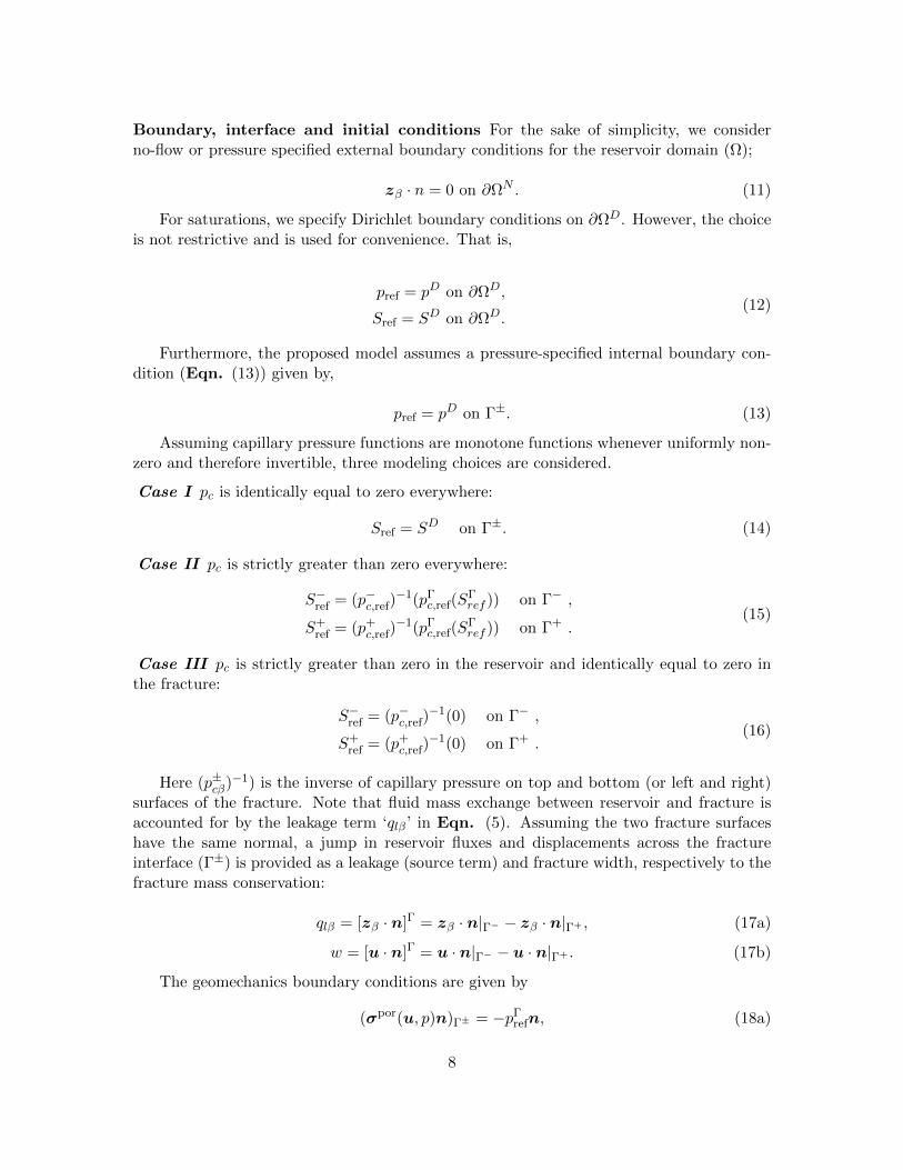
reservoir domain and a lubrication equation for the fractures. We further assume oil andwater are the two phases denoted by subscripts o and w, respectively. A schematic of afractured reservoir is shown in Fig. 3. Note that the fracture geometry is not necessarilyplanar and as explained later, our numerical method allows for non-planar geometries.

We treat the fracture as a pressure specified internal boundary in the reservoir domainand provide the jump in flux across this interface as a leakage term to the fracture. Thefracture pressure is also treated as an internal traction boundary condition for the reservoirgeomechanics. The resulting jump in displacements (fracture width or aperture) is used tocalculate fracture permeability. For the model description, we consider a fractured reservoirdomain (Ω) where the fracture is represented as an interface (Γ) with two surfaces (Γ±),as shown in Fig. 3. Here ∂ΩN and ∂ΩD represent the Neumann and Dirichlet parts,respectively of the external boundary of the reservoir domain Ω.

5

0 0.2 0.4 0.6 0.8 10

0.05

0.1

0.15

0.2

0.25

0.3

0.35

Sw

kro

, k

rw

kro

krw

Figure 2: Relative permeability curves for oil and water phases.

Ω

!"#

!"$ ∂Ω

N

∂ΩD

Figure 3: Schematic of a fractured reservoir flow model.

Equations in the reservoir (Ω\Γ) We begin by describing the flow equations everywhereexcept for the fracture interface Γ.

Flow equations The mass-conservation equation for the phase β reads,

∂

∂t(φ∗Sβρβ) +∇ · zβ = qβ. (1)

Here, φ∗ is the fluid fraction, Sβ the saturation, ρβ the density, zβ the flux of phase β = o(oil phase), w (water phase). The source/sink term qβ is treated using an appropriate wellmodel (Peaceman (1978)). The Darcy equation relates the flux zβ to the gradient of thephase pressure and is given by

zβ = −Kρβkrβνβ

(∇pβ − ρβg) . (2)

In the above, K is a full tensor absolute permeability, krβ the relative permeability, and νβthe viscosity of phase β. The second term in the parenthesis models the effect of gravity.

Mechanics The displacement u of the porous medium is described by the quasistaticporoelastic equations. Eqn. (3) represents the momentum conservation (force balance)and Eqn. (4) the constitutive equation relating stress (σpor) and displacements (u):

−∇ · σpor(u, pref) = f , (3a)

6

f =

ρs(1− φ∗) + φ∗∑β

ρβSβ

g, (3b)

φ∗ = φo + α∇ · u+1

Mpref. (3c)

σpor(u, pref) = σ(u)− αprefI, (4a)

σ(u) = λ(∇ · u)I + 2µε(u), (4b)

ε(u) =1

2(∇u+∇uT ). (4c)

Here, σpor is the Cauchy stress tensor, ε the strain tensor, f the body force, ρs density ofthe solid matrix, g acceleration due to gravity, α the Biot coefficient, pref the reference phasepressure, I the identity matrix, φo the reference porosity, µ and λ are Lame parameters.

Equations in the fracture (Γ) A lubrication equation is assumed as the constitutiverelation between fracture fluxes (zΓ

β) and gradient of fracture pressure (pΓ). Here, the

fracture gradient (∇) and divergence (∇·) operators are defined on a lower dimensionalspace (Rd−1). Eqns. (5) and (6) represent the mass conservation and Darcy’s law for thephase ‘β’ in the fracture domain:

∂

∂t

(wSΓ

βρΓβ

)+ w∇ · zΓ

β = qΓβ + qlβ, (5)

zΓβ = −KΓρΓ

β

krβνβ

(∇pΓ

β − ρΓβg). (6)

Here, qlβ is the fracture leakage term as defined below. The absolute permeability KΓ

is given by Eqn. (7) where (w) is the fracture width,

KΓ =w2

12. (7)

Closure conditions A slightly compressible, equation of state relating fluid densities andpressures is assumed (Eqn. (8)) for both reservoir and fracture. Further, the capillarypressure and saturation constraints are given by Eqns. (9) and (10), respectively. Forsimplicity of notation we let ? = Ω\Γ or Γ and for a given function fΩ\Γ to be equal to f.Thus, we have

ρ?β = ρβ0

[1 + cβ(p?ref + p?cβ − p0)

], (8)

p?cβ(S?β) = p?o − p?w, (9)

S?w + S?o = 1. (10)

Here, cβ is the fluid compressibility, pcβ the capillary pressure for the fluid phase β andSref the reference phase saturation. The relative permeabilities are continuous functions ofreference phase saturation (Sref) for both reservoir and fracture. A more general table basedcapillary pressure and relative permeability curve description has also been implemented.

7

Boundary, interface and initial conditions For the sake of simplicity, we considerno-flow or pressure specified external boundary conditions for the reservoir domain (Ω);

zβ · n = 0 on ∂ΩN . (11)

For saturations, we specify Dirichlet boundary conditions on ∂ΩD. However, the choiceis not restrictive and is used for convenience. That is,

pref = pD on ∂ΩD,

Sref = SD on ∂ΩD.(12)

Furthermore, the proposed model assumes a pressure-specified internal boundary con-dition (Eqn. (13)) given by,

pref = pD on Γ±. (13)

Assuming capillary pressure functions are monotone functions whenever uniformly non-zero and therefore invertible, three modeling choices are considered.

Case I pc is identically equal to zero everywhere:

Sref = SD on Γ±. (14)

Case II pc is strictly greater than zero everywhere:

S−ref = (p−c,ref)−1(pΓ

c,ref(SΓref )) on Γ− ,

S+ref = (p+

c,ref)−1(pΓ

c,ref(SΓref )) on Γ+ .

(15)

Case III pc is strictly greater than zero in the reservoir and identically equal to zero inthe fracture:

S−ref = (p−c,ref)−1(0) on Γ− ,

S+ref = (p+

c,ref)−1(0) on Γ+ .

(16)

Here (p±cβ)−1) is the inverse of capillary pressure on top and bottom (or left and right)surfaces of the fracture. Note that fluid mass exchange between reservoir and fracture isaccounted for by the leakage term ‘qlβ’ in Eqn. (5). Assuming the two fracture surfaceshave the same normal, a jump in reservoir fluxes and displacements across the fractureinterface (Γ±) is provided as a leakage (source term) and fracture width, respectively to thefracture mass conservation:

qlβ = [zβ · n]Γ = zβ · n|Γ− − zβ · n|Γ+ , (17a)

w = [u · n]Γ = u · n|Γ− − u · n|Γ+ . (17b)

The geomechanics boundary conditions are given by

(σpor(u, p)n)Γ± = −pΓrefn, (18a)

8

[σpor(u, p)n]Γ = 0, (18b)

u = 0 on ∂ΩDs , (18c)

σporn = σN on ∂ΩNs , (18d)

where ∂Ωs are the external boundaries. The initial conditions at time t = 0 are as follows:

pref = p0, (19)

Sref = S0, (20)

u = u0. (21)

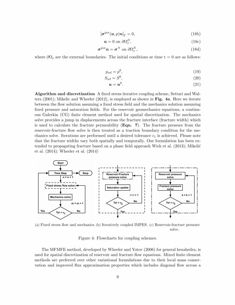
Algorithm and discretization A fixed stress iterative coupling scheme, Settari and Wal-ters (2001); Mikelic and Wheeler (2012), is employed as shown in Fig. 4a. Here we iteratebetween the flow solution assuming a fixed stress field and the mechanics solution assumingfixed pressure and saturation fields. For the reservoir geomechanics equations, a continu-ous Galerkin (CG) finite element method used for spatial discretization. The mechanicssolve provides a jump in displacements across the fracture interface (fracture width) whichis used to calculate the fracture permeability (Eqn. 7). The fracture pressure from thereservoir-fracture flow solve is then treated as a traction boundary condition for the me-chanics solve. Iterations are performed until a desired tolerance ε1 is achieved. Please notethat the fracture widths vary both spatially and temporally. Our formulation has been ex-tended to propagating fracture based on a phase field approach Wick et al. (2013); Mikelicet al. (2014); Wheeler et al. (2014)

Start

Fixed stress flow solve

Tol < ϵ1Yes

Time Step

No

Stop

n = n + 1

Mechanics solve

m = m + 1

(a) Fixed stress flow and mechanics.

Reservoir-Fracture pressure solve

Tol < ϵ2

Yes

No

l = l + 1

Saturation update

(b) Iteratively coupled IMPES.

Reservoir pressure solve

Tol < ϵ3

Yes

No

k = k + 1

Fracture pressure solve

(c) Reservoir-fracture pressuresolve.

Figure 4: Flowcharts for coupling schemes.

The MFMFE method, developed by Wheeler and Yotov (2006) for general hexahedra, isused for spatial discretization of reservoir and fracture flow equations. Mixed finite elementmethods are preferred over other variational formulations due to their local mass conser-vation and improved flux approximation properties which includes diagonal flow across a

9

grid-block. An appropriate choice of mixed finite element spaces and degrees of freedombased upon the quadrature rule for numerical integration (Wheeler et al. (2011b); Wheelerand Xue (2011)) allow flux degrees of freedoms to be defined in terms of cell-centered grid-block pressures adjacent to the vertex. A 9 and 27 point pressure stencil is formed forlogically rectangular 2D and 3D grids, respectively.

The flow equations are solved using an iteratively-coupled, implicit pressure explicitsaturation (IC-IMPES) scheme as shown in Fig. 4b. The reference phase pressure issolved implicitly by solving the total mass conservation equation with a backward Eulertime discretization assuming the reference phase saturations are given. This is followed byan explicit update of reference phase saturations using a forward Euler time discretizationfor the phase mass conservation equation. The solution algorithm allows for smaller satura-tion time-step sizes than pressure time-steps. Further, the Courant-Frederichs-Lewy (CFL)condition on the explicit saturation updates are then obeyed using different time-step sizesfor the reservoir and the fracture. The fluid property data for intermediate saturation timesteps are calculated by linear interpolation of pressure. The demarcation of reservoir andfracture as separate domains allows for special treatment of computationally challengingregions. Please note that since the pressures are solved implicitly, there are no restrictionson the pressure time-step size. A tolerance of ε2 determines convergence of the iterativescheme.

We finally turn our attention to the non-linear, reservoir-fracture flow system. Thereservoir pressure solve provides a jump in fluxes across the fracture interface. These in turnact as source/sink terms for the fracture pressure solve. The resulting fracture pressure isthen treated as a pressure specified internal boundary for the reservoir domain. We couplethe reservoir and fracture pressure solves by iterating between the two implicit systemsuntil a desired tolerance ε3 is reached. Fig. 4c provides an outline of the coupled reservoir-fracture flow model used in this work.

Results

In this section, we consider a number of numerical experiments to demonstrate ourmodeling and computational approaches. We begin with validation of the coupled reservoir-fracture flow model by comparing with physical experimental results for spontaneous im-bibition of the wetting phase. The second numerical experiment studies the significanceof fracture orientations for recovery processes in a reservoir. An injection scenario for amulti-stage hydraulic fracture is shown in the third example. The fourth example demon-strates stress field reorientations for injection and production from a hydraulic fracture.Finally, a field case for Frio Juntunen and Wheeler (2012)) is presented showing long termproduction from a fractured reservoir with multiple injection and production wells. Thenumerical experiments have been conducted for both lab scale as well as field scale. Pleasenote that the fracture aperture (or width) is time invariant and varies spatially from 1 mm- 3 mm along the fracture length in all numerical experiments except example 4. For thecouple flow and mechanics the above is used as an initial guess since fracture widths varyspatially and temporally and are solved as a part of the system of equations.

Capillary imbibition in a fractured core We compare the results of our numericalmodel to experimental data, given by Karpyn (2005), for a fractured Berea sandstonecore. The core is initially saturated only with water (Sw = 1.0) followed by a primary

10

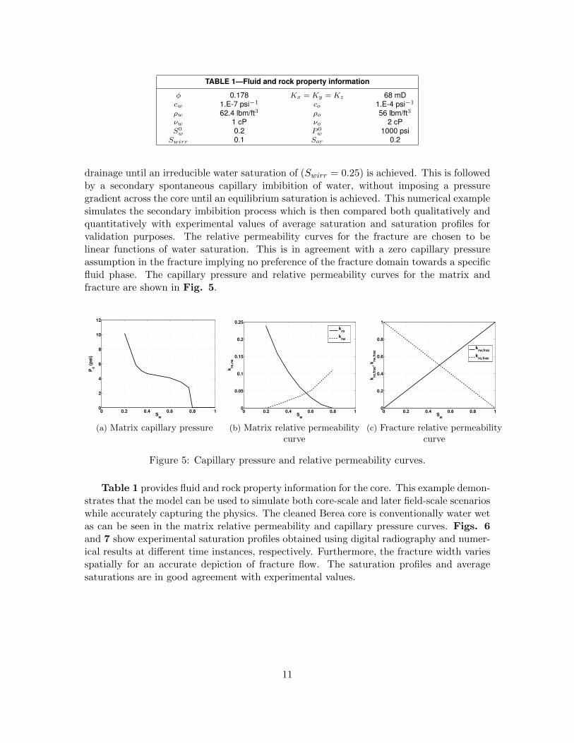
TABLE 1—Fluid and rock property information

φ 0.178 Kx = Ky = Kz 68 mDcw 1.E-7 psi−1 co 1.E-4 psi−1

ρw 62.4 lbm/ft3 ρo 56 lbm/ft3νw 1 cP νo 2 cPS0w 0.2 P 0

w 1000 psiSwirr 0.1 Sor 0.2

drainage until an irreducible water saturation of (Swirr = 0.25) is achieved. This is followedby a secondary spontaneous capillary imbibition of water, without imposing a pressuregradient across the core until an equilibrium saturation is achieved. This numerical examplesimulates the secondary imbibition process which is then compared both qualitatively andquantitatively with experimental values of average saturation and saturation profiles forvalidation purposes. The relative permeability curves for the fracture are chosen to belinear functions of water saturation. This is in agreement with a zero capillary pressureassumption in the fracture implying no preference of the fracture domain towards a specificfluid phase. The capillary pressure and relative permeability curves for the matrix andfracture are shown in Fig. 5.

0 0.2 0.4 0.6 0.8 10

2

4

6

8

10

12

Sw

Pc (

ps

i)

(a) Matrix capillary pressure

0 0.2 0.4 0.6 0.8 10

0.05

0.1

0.15

0.2

0.25

Sw

kro

,rw

kro

krw

(b) Matrix relative permeabilitycurve

0 0.2 0.4 0.6 0.8 10

0.2

0.4

0.6

0.8

1

Sw

kro

,fra

c, k

rw,f

rac

krw,frac

kro,frac

(c) Fracture relative permeabilitycurve

Figure 5: Capillary pressure and relative permeability curves.

Table 1 provides fluid and rock property information for the core. This example demon-strates that the model can be used to simulate both core-scale and later field-scale scenarioswhile accurately capturing the physics. The cleaned Berea core is conventionally water wetas can be seen in the matrix relative permeability and capillary pressure curves. Figs. 6and 7 show experimental saturation profiles obtained using digital radiography and numer-ical results at different time instances, respectively. Furthermore, the fracture width variesspatially for an accurate depiction of fracture flow. The saturation profiles and averagesaturations are in good agreement with experimental values.

11

Figure 6: Experimental saturation profiles from Karpyn (2005) using digital radiographyat different times

Figure 7: Numerical saturation profiles (left to right)

Discrete natural fractures In the introduction section, we presented a single fractureexample to motivate a detailed interface based modeling approach. In the introduction, wepresented an example (Fig. 1) where the saturation front channeled through the fracturethereby reducing sweep area. Here, we present a similar case with two discrete fracturesin a reservoir domain of size 10 ft× 10 ft (approximately) with bottom-hole pressure spec-ified injection (520 psi) and production (500 psi) wells located at diagonally opposite ends.The reservoir and fluid property data along with initial and boundary conditions remainunchanged.

12

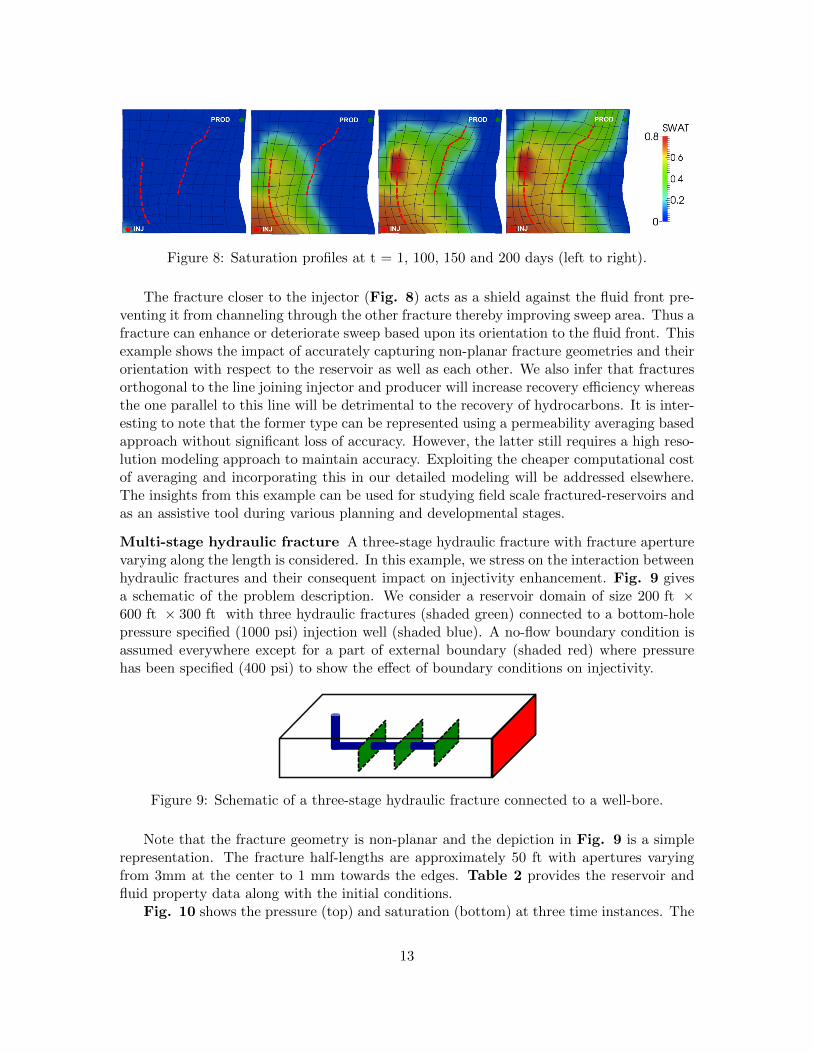
Figure 8: Saturation profiles at t = 1, 100, 150 and 200 days (left to right).

The fracture closer to the injector (Fig. 8) acts as a shield against the fluid front pre-venting it from channeling through the other fracture thereby improving sweep area. Thus afracture can enhance or deteriorate sweep based upon its orientation to the fluid front. Thisexample shows the impact of accurately capturing non-planar fracture geometries and theirorientation with respect to the reservoir as well as each other. We also infer that fracturesorthogonal to the line joining injector and producer will increase recovery efficiency whereasthe one parallel to this line will be detrimental to the recovery of hydrocarbons. It is inter-esting to note that the former type can be represented using a permeability averaging basedapproach without significant loss of accuracy. However, the latter still requires a high reso-lution modeling approach to maintain accuracy. Exploiting the cheaper computational costof averaging and incorporating this in our detailed modeling will be addressed elsewhere.The insights from this example can be used for studying field scale fractured-reservoirs andas an assistive tool during various planning and developmental stages.

Multi-stage hydraulic fracture A three-stage hydraulic fracture with fracture aperturevarying along the length is considered. In this example, we stress on the interaction betweenhydraulic fractures and their consequent impact on injectivity enhancement. Fig. 9 givesa schematic of the problem description. We consider a reservoir domain of size 200 ft ×600 ft × 300 ft with three hydraulic fractures (shaded green) connected to a bottom-holepressure specified (1000 psi) injection well (shaded blue). A no-flow boundary condition isassumed everywhere except for a part of external boundary (shaded red) where pressurehas been specified (400 psi) to show the effect of boundary conditions on injectivity.

Figure 9: Schematic of a three-stage hydraulic fracture connected to a well-bore.

Note that the fracture geometry is non-planar and the depiction in Fig. 9 is a simplerepresentation. The fracture half-lengths are approximately 50 ft with apertures varyingfrom 3mm at the center to 1 mm towards the edges. Table 2 provides the reservoir andfluid property data along with the initial conditions.

Fig. 10 shows the pressure (top) and saturation (bottom) at three time instances. The

13

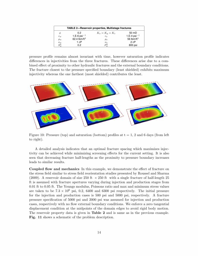
TABLE 2—Reservoir properties, Multistage fractures

φ 0.2 Kx = Ky = Kz 50 mDcw 1.E-6 psi−1 co 1.E-4 psi−1

ρw 62.4 lbm/ft3 ρo 56 lbm/ft3νw 1 cP νo 2 cPS0w 0.2 P 0

w 800 psi

pressure profile remains almost invariant with time, however saturation profile indicatesdifferences in injectivities from the three fractures. These differences arise due to a com-bined effect of proximity to other hydraulic fractures and the external boundary conditions.The fracture closest to the pressure specified boundary (least shielded) exhibits maximuminjectivity whereas the one farthest (most shielded) contributes the least.

Figure 10: Pressure (top) and saturation (bottom) profiles at t = 1, 2 and 6 days (from leftto right).

A detailed analysis indicates that an optimal fracture spacing which maximizes injec-tivity can be achieved while minimizing screening effects for the current setting. It is alsoseen that decreasing fracture half-lengths as the proximity to pressure boundary increasesleads to similar results.

Coupled flow and mechanics In this example, we demonstrate the effect of fracture onthe stress field similar to stress field reorientation studies presented by Roussel and Sharma(2009). A reservoir domain of size 250 ft × 250 ft with a single fracture of half-length 25ft is assumed with fracture apertures varying during injection and production stages from0.01 ft to 0.05 ft. The Youngs modulus, Poissons ratio and max and minimum stress valuesare taken to be 7.3 × 106 psi, 0.2, 6400 and 6300 psi respectively. The initial pressurefor the injection and production cases is 500 psi and 5000 psi, respectively. A fracturepressure specification of 5000 psi and 2000 psi was assumed for injection and productioncases, respectively with no flow external boundary conditions. We enforce a zero tangentialdisplacement condition at the midpoints of the domain edges to avoid rigid body motion.The reservoir property data is given in Table 2 and is same as in the previous example.Fig. 11 shows a schematic of the problem description.

14

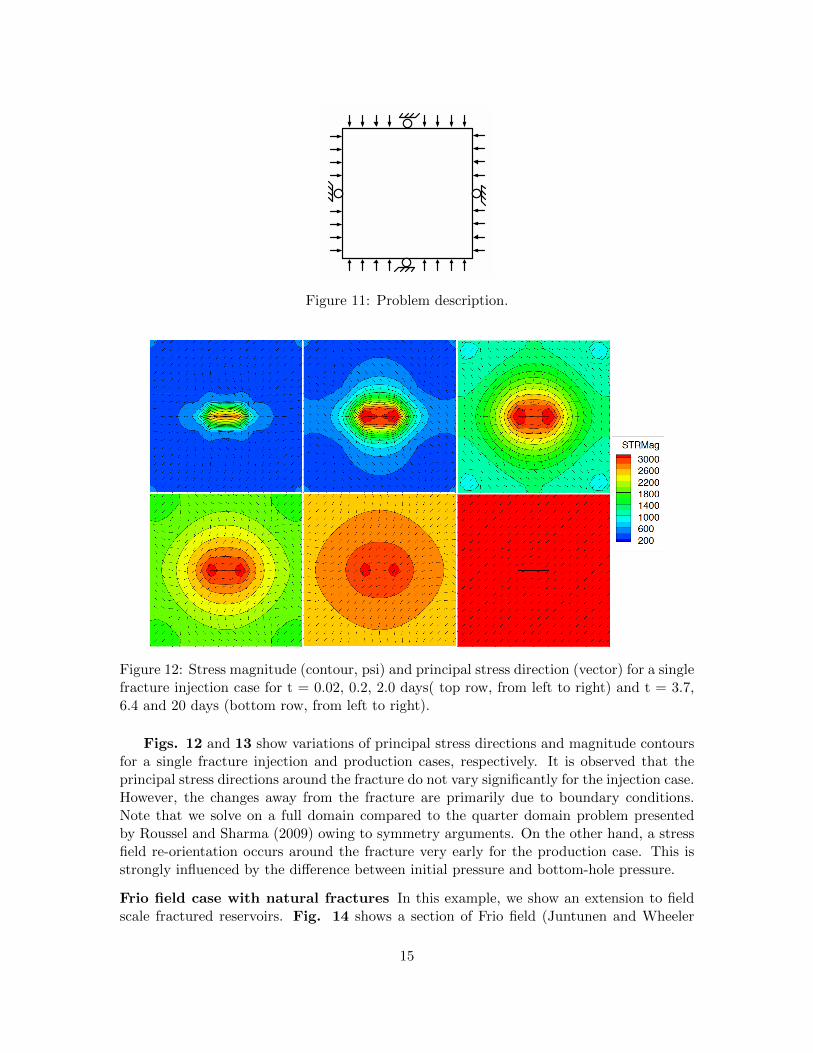
Figure 11: Problem description.

Figure 12: Stress magnitude (contour, psi) and principal stress direction (vector) for a singlefracture injection case for t = 0.02, 0.2, 2.0 days( top row, from left to right) and t = 3.7,6.4 and 20 days (bottom row, from left to right).

Figs. 12 and 13 show variations of principal stress directions and magnitude contoursfor a single fracture injection and production cases, respectively. It is observed that theprincipal stress directions around the fracture do not vary significantly for the injection case.However, the changes away from the fracture are primarily due to boundary conditions.Note that we solve on a full domain compared to the quarter domain problem presentedby Roussel and Sharma (2009) owing to symmetry arguments. On the other hand, a stressfield re-orientation occurs around the fracture very early for the production case. This isstrongly influenced by the difference between initial pressure and bottom-hole pressure.

Frio field case with natural fractures In this example, we show an extension to fieldscale fractured reservoirs. Fig. 14 shows a section of Frio field (Juntunen and Wheeler

15

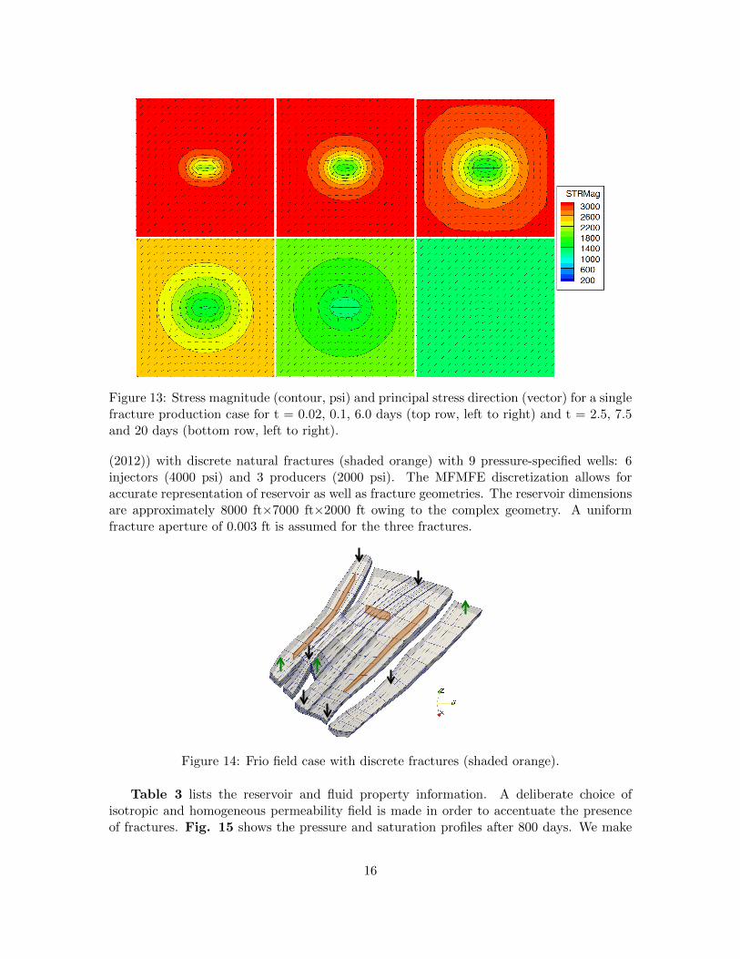
Figure 13: Stress magnitude (contour, psi) and principal stress direction (vector) for a singlefracture production case for t = 0.02, 0.1, 6.0 days (top row, left to right) and t = 2.5, 7.5and 20 days (bottom row, left to right).

(2012)) with discrete natural fractures (shaded orange) with 9 pressure-specified wells: 6injectors (4000 psi) and 3 producers (2000 psi). The MFMFE discretization allows foraccurate representation of reservoir as well as fracture geometries. The reservoir dimensionsare approximately 8000 ft×7000 ft×2000 ft owing to the complex geometry. A uniformfracture aperture of 0.003 ft is assumed for the three fractures.

Figure 14: Frio field case with discrete fractures (shaded orange).

Table 3 lists the reservoir and fluid property information. A deliberate choice ofisotropic and homogeneous permeability field is made in order to accentuate the presenceof fractures. Fig. 15 shows the pressure and saturation profiles after 800 days. We make

16

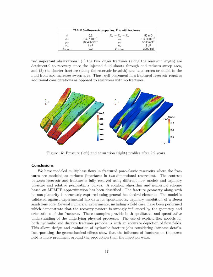
TABLE 3—Reservoir properties, Frio with fractures

φ 0.2 Kx = Ky = Kz 50 mDcw 1.E-7 psi−1 co 1.E-4 psi−1

ρw 62.4 lbm/ft3 ρo 56 lbm/ft3νw 1 cP νo 2 cP

Sw,init 0.2 Pw,init 3000 psi

two important observations: (1) the two longer fractures (along the reservoir length) aredetrimental to recovery since the injected fluid shoots through and reduces sweep area,and (2) the shorter fracture (along the reservoir breadth) acts as a screen or shield to thefluid front and increases sweep area. Thus, well placement in a fractured reservoir requiresadditional considerations as opposed to reservoirs with no fractures.

Figure 15: Pressure (left) and saturation (right) profiles after 2.2 years.

Conclusions

We have modeled multiphase flows in fractured poro-elastic reservoirs where the frac-tures are modeled as surfaces (interfaces in two-dimensional reservoirs). The contrastbetween reservoir and fracture is fully resolved using different flow models and capillarypressure and relative permeability curves. A solution algorithm and numerical schemebased on MFMFE approximation has been described. The fracture geometry along withits non-planarity is accurately captured using general hexahedral elements. The model isvalidated against experimental lab data for spontaneous, capillary imbibition of a Bereasandstone core. Several numerical experiments, including a field case, have been performedwhich demonstrate that the recovery pattern is strongly influenced by the geometry andorientations of the fractures. These examples provide both qualitative and quantitativeunderstanding of the underlying physical processes. The use of explicit flow models forboth hydraulic and discrete fractures provide us with an accurate depiction of flow fields.This allows design and evaluation of hydraulic fracture jobs considering intricate details.Incorporating the geomechanical effects show that the influence of fractures on the stressfield is more prominent around the production than the injection wells.

17

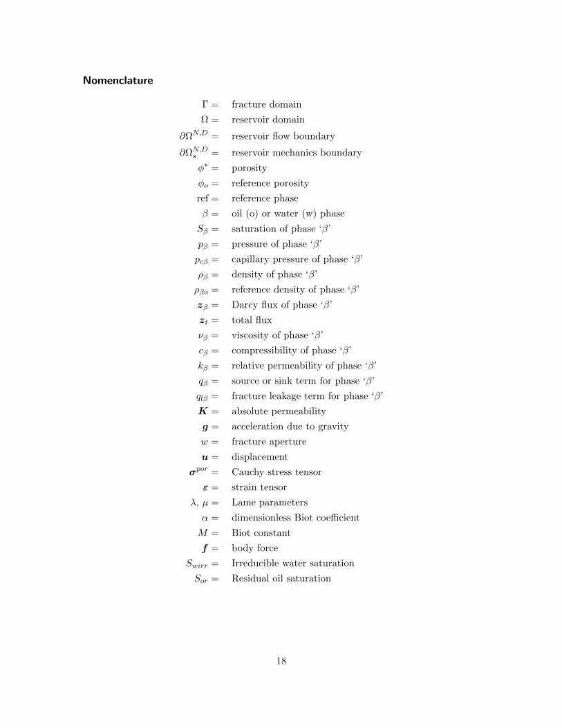
Nomenclature

Γ = fracture domain

Ω = reservoir domain

∂ΩN,D = reservoir flow boundary

∂ΩN,Ds = reservoir mechanics boundary

φ∗ = porosity

φo = reference porosity

ref = reference phase

β = oil (o) or water (w) phase

Sβ = saturation of phase ‘β’

pβ = pressure of phase ‘β’

pcβ = capillary pressure of phase ‘β’

ρβ = density of phase ‘β’

ρβo = reference density of phase ‘β’

zβ = Darcy flux of phase ‘β’

zt = total flux

νβ = viscosity of phase ‘β’

cβ = compressibility of phase ‘β’

kβ = relative permeability of phase ‘β’

qβ = source or sink term for phase ‘β’

qlβ = fracture leakage term for phase ‘β’

K = absolute permeability

g = acceleration due to gravity

w = fracture aperture

u = displacement

σpor = Cauchy stress tensor

ε = strain tensor

λ, µ = Lame parameters

α = dimensionless Biot coefficient

M = Biot constant

f = body force

Swirr = Irreducible water saturation

Sor = Residual oil saturation

18

Acknowledgements

This research was funded by ConocoPhillips grant UTA10-000444, DOE grant ER25617,Saudi Aramco grant UTA11-000320 and Statoil grant UTA13-000884. In addition, thesecond author has been supported by an ICES postdoctoral fellowship and a HumboldtFeodor Lynen fellowship. The authors would like to express their sincere thanks for thefunding.

References

Al-Hinai, O. A., Singh, G., Almani, T. M., Pencheva, G., and Wheeler, M. F., 2013. Mod-eling multiphase flow with nonplanar fractures. SPE Reservoir Simulation Symposium,Woodlands, TX.

Arbogast, T., Wheeler, M. F., and Yotov, I., 1997. Mixed finite elements for elliptic problemswith tensor coefficients as cell-centered finite differences. SIAM Journal on NumericalAnalysis, 34 (2): 828–852.

Bastian, P., Chen, Z., Ewing, R., Helmig, R., Jakobs, H., and Reichenberger, V., 2000.Numerical simulation of multiphase-flow in fractured porous media, volume 522 of LectureNotes in Physics. Springer.

Biot, M. A., 1941a. Consolidation Settlement Under a Rectangular Load Distribution.Journal of applied physics, 12 (5): 426.

Biot, M. A., 1941b. General theory of threedimensional consolidation. Journal of appliedphysics, 12 (2): 155–164.

Biot, M. A., 1955. Theory of Elasticity and Consolidation for a Porous Anisotropic Solid.Journal of applied physics, 26 (2): 182.

Dean, R. H., Gai, X., Stone, C. M., and Minkoff, S. E., 2006. A comparison of techniquesfor coupling porous flow and geomechanics. SPE Journal, 11 (1): 132–140.

Frih, N., Roberts, J. E., and Saada, A., 2008. Modeling fractures as interfaces: a model forForchheimer fractures. Computational Geosciences, 12 (1): 91–104.

Ganis, B., Girault, V., Mear, M., Singh, G., and Wheeler, M., 2013. Modeling Fracturesin a Poro-Elastic Medium. Oil & Gas Science and Technology – Revue d’IFP Energiesnouvelles.

Girault, V., Wheeler, M. F., Ganis, B., and Mear, M., 2013. A lubrication fracture modelin a poro-elastic medium. ICES Report, 1–54.

Grillo, A., Logashenko, D., Stichel, S., and Wittum, G., 2010. Simulation of density-drivenflow in fractured porous media. Advances in Water Resources, 33 (12): 1494–1507.

Hoteit, H. and Firoozabadi, A., 2005. Multicomponent fluid flow by discontinuous Galerkinand mixed methods in unfractured and fractured media. Water Resources Research,41 (11): n/a–n/a.

19

Hoteit, H. and Firoozabadi, A., 2006. Compositional modeling of discrete-fractured me-dia without transfer functions by the discontinuous Galerkin and mixed methods. SPEJournal, 11 (3): 341–352.

Hoteit, H. and Firoozabadi, A., 2008a. An efficient numerical model for incompressibletwo-phase flow in fractured media. Advances in Water Resources, 31 (6): 891–905.

Hoteit, H. and Firoozabadi, A., 2008b. Numerical modeling of two-phase flow in heteroge-neous permeable media with different capillarity pressures. Advances in Water Resources,31 (1): 56–73.

Ingram, R., Wheeler, M. F., and Yotov, I., 2010. A Multipoint Flux Mixed Finite ElementMethod on Hexahedra. SIAM Journal on Numerical Analysis, 48 (4): 1281–1312.

Juntunen, M. and Wheeler, M., 2012. Two-phase flow in complicated geometries. Compu-tational Geosciences, 17 (2).

Karpyn, Z. T., 2005. Capillary-driven Flow in Fractured Sandstone.

Kim, J., Sonnenthal, E. L., and Rutqvist, J., 2012. Formulation and sequential numericalalgorithms of coupled fluid/heat flow and geomechanics for multiple porosity materials.International Journal for Numerical Methods in Engineering, 92 (5): 425–456.

Martin, V., Jaffre, J., and Roberts, J. E., 2005. Modeling Fractures and Barriers as In-terfaces for Flow in Porous Media. SIAM Journal on Scientific Computing, 26 (5):1667–1691.

Mikelic, A., Wang, B., and Wheeler, M. F., 2014. Numerical convergence study of iterativecoupling for coupled flow and geomechanics. Computational Geosciences.

Mikelic, A., Wheeler, M., and Wick, T., 2014. A phase-field method for propagating fluid-filled fractures coupled to a surrounding porous medium. ICES Report 14-08, submittedfor publication.

Mikelic, A. and Wheeler, M. F., 2012. Convergence of iterative coupling for coupled flowand geomechanics. Computational Geosciences, 17 (3): 455–461.

Monteagudo, J. and Firoozabadi, A., 2007. Control-volume model for simulation of waterinjection in fractured media: incorporating matrix heterogeneity and reservoir wettabilityeffects. SPE Journal, 12 (3): 355–366.

Monteagudo, J. E. P. and Firoozabadi, A., 2004. Control-volume method for numericalsimulation of two-phase immiscible flow in two- and three-dimensional discrete-fracturedmedia. Water Resources Research, 40 (7): n/a–n/a.

Peaceman, D. W., 1978. Interpretation of Well-Block Pressures in Numerical ReservoirSimulation. Old SPE Journal, 18 (03): 183–194.

Roussel, N. and Sharma, M., 2009. Quantifying transient effects in altered-stress refractur-ing of vertical wells. SPE Hydraulic Fracturing Technology Conference.

20

Settari, A. and Walters, D. A., 2001. Advances in coupled geomechanical and reservoirmodeling with applications to reservoir compaction. SPE Journal, 6 (3): 334–342.

Terzaghi, K., 1943. Theoretical soil mechanics. J. Wiley, New York.

Wheeler, M., Wick, T., and Wollner, W., 2014. An augmented-Lagangrian method for thephase-field approach for pressurized fractures. Comp. Meth. Appl. Mech. Engrg., 271:69–85.

Wheeler, M., Xue, G., and Yotov, I., 2011a. Accurate cell-centered discretizations formodeling multiphase flow in porous media on general hexahedral and simplicial grids.SPE Reservoir Simulation Symposium.

Wheeler, M. F. and Xue, G., 2011. Accurate locally conservative discretizations for modelingmultiphase flow in porous media on general hexahedra grids. Proceedings of the 12thEuropean Conference on the Mathematics of Oil Recovery-ECMOR XII, publisher EAGE.

Wheeler, M. F., Xue, G., and Yotov, I., 2011b. A Family of Multipoint Flux Mixed FiniteElement Methods for Elliptic Problems on General Grids. Procedia Computer Science,4: 918–927.

Wheeler, M. F. and Yotov, I., 2006. A Multipoint Flux Mixed Finite Element Method.SIAM Journal on Numerical Analysis, 44 (5): 2082–2106.

Wick, T., Singh, G., and Wheeler, M., 2013. Pressurized fracture propagation using aphase-field approach coupled to a reservoir simulator. SPE 168597-MS, SPE Proc.

21