ic file copy - defense technical information center · " ic file copy tritium method oil ... i...
TRANSCRIPT
" iC FILE COPY
TRITIUM METHOD OIL CONSUMPTION AND ITS RELATION TO OIL FILM
THICKNESSES IN A PRODUCTION DIESEL ENGINE
(0by 11RICHARD M. HARTMAN ELECTE
B.S., United States Naval Academy SEP 2 5 1990(1985) .
SUBMITTED TO THE DEPARTMENT OF D cOCEAN ENGINEERINGIN PARTIAL FULFILLMENT OF THE REQU IREMENTS
FOR THE DEGREES OFMASTER OF SCIENCE IN NAVAL ARCHITECTURE/MARINE ENGINEERING
and
MASTER OF SCIENCE IN MECHANICAL ENGINEERING
at the R1- -G-Os-&oMA-SSACHUSETT7S INSTITUTE OF TECHNOLOGY
/VP.S June, 1990
© Massachusetts Institute of Technology, 1990. All rights reserved
The author hereby grants to MIT and the U.S. G vemment permission toreproduce and to distribu)e-c pies this tl esis c nt in whole or in pan.
Signature of Author ~ <-7Department of Ocean Engineering
May 1990
Certified byDr. David P. Hoult
Senior Research AssociateCertified by - ' ,/' - /Thesis Supervisor
Professor A. Douglas CarmichaelThesis Reader
Accepted by (,, /old ~ keA'<RDouglas Carmichael, Chairman
Departmental Committee on Graduate Studiesnt of Ocean Engineering
Accepted byA. A. Sonin, Chainrman
I ---.TI- ?. NT A" Departmental Committee on Graduate StudiesDepartment of Mechamical Engineering/:.!:h releasoe
L0 9 2ted
90 09 24 059
2
TRITIUM NIET1t(D OIL CONSUMPTION AND ITS RELATION TO OILFILM THICKNESSES IN A PRODUCTION DIESEL ENGINE
by
RICHARD M. HARTMAN
Submitted to the Department of Ocean Engineering in partial fulfillment of the requirementsfor the degrees of Master of Science i-. Naval Architecture/Marine Engineering and Master
of Science in Mechanical Engineering
ABSTRACT
Oil consumption was measured in a modem production diesel engine using tritium as aradiotracer. The measurements were made primarily at two speeds and one load using firsta single-grade lubricant and then a multi-grade lubricant.
These values were then compared to oil flow rates up/down the liner which were basedon film thickness traces of a sister engine wider the same loads and speeds. The traceswere obtained using the laser-fluorescence technique. For the most part, it was discoveredthat there does not seem to exist a correlation between these flow rates and oilconsumption. However, the traces do reveal that the crown land is dry on all four strokesand thus does not contribute to the engine's oil consumption.
A larger data base is necessary in order to ,curately compare oil consumption to thefilm traces. This is currently in progress as of this writing. (
Thesis Supervisor: David P. HoultTitle: Senior Research Associate
Department of Mechanical Engineering
3
ACKNOWLEDGEMENTS
I could not have submitted this thesis without the help, guidance, and support of thefollowing:
First, I would like to thank both Professor John B. Heywood for getting me started atthe Sloan Automotive Laboratory and, of course, Dr. David P. Hoult. As my advisor, Dr.Hoult was extremely enthusiastic and was consistently able to encourage and guide me tocompletion.
There are others connected with the Sloan Lab who also deserve a great deal of thanks.For instance, Don Fitzgerald and Brian Corkum were both instrumental in the acquisitionand installation of both my engine and the required hardware. I am grateful to them for thisand also to fellow students, Mark Olechowski and Matthew Bliven, who assisted me in mywork on the computer. A special thanks, however, goes to Matthew Bliven, withoutwhom, my data analysis would have been non-existent.
The men and women of MIT's Radiation Protection Office were extremely helpful inmeasuring the radioactive levels of my samples. I could always count on having a quickturn around of the results.
Procedures for the tritium method were supplied by the Sealed Power Corporation.They assisted greatly in getting the experiment off the ground.
The love and support that I got from my family was very important. They kept megoing over the two years and, as always, were there when I needed them.
Lastly, and most importantly, I thank God, through whom all things are possible.
. .. . r
D I
DistI
-IL

4
TABLE 01F CONTENIS
TITLE PAGE ................................................ 1
A B S T R A C T ........................................................................................
ACKNOWLEDGEMENTS ...................................... 3
TABLE OF CONTENTS ...................................... 4
LIST OF TABLES ........................................... 7
LIST OF FIGURES .........................................
CHAPTER 1 BACKGROUND AND INTRODUCTION ............................. 10
CHAPTER 2 DESCRIPTION OF MEASURING TECHNIQUE ........................ 11
2.1 BASIC METHOD .................................. 1
2.2 SOOT SAM PLE COLLECTION ................................................ I1
2.3 LIQUID SCINTILLATION COUNTING ................................. 12
CHAPTER 3 EQUIPM ENT AND SET-UP ................................................. 13
3.1 ENGINE ........................... 13
3.2 RADIOACTIVE LUBRICATING OILS .................................... 13
3.3 ENGINE INSTRUMENTATION ............................................ 13
3.4 DESCRIPTION OF PISTON AND RINGS ............................... 14
3.5 SAM PLING SYSTEM ....................................................... 14
3.6 OIL FILM THICKNESS MEASUREMENTS ............................. 15
CHAPTER 4 DESCRIPTION OF EXPERIMENTS ................................... 16
4.1 PR O C ED U R ES ................................................................ 16
4.2 ENGINE OPERATIONG CONDITIONS ................................... 16
CHAPTER 5 GRAPHIC RESULTS ..................................................... 17
5.1 OIL CONSUMPTION MEASUREMENTS ................................ 17
5.2 OIL FILM THICKNESSES ................................................. 17
CHAPTER 6 HYPOTHESES AND ANALYSIS ....................................... 18
6 .1 H Y P O T H E S E S ..................................................................... 18
5
6.2 ANALYSIS AND DISCUSSION ............................................ 19
6.3 PROBABLE ERRORS IN ANALYSIS TECHNIQUE ................... 23
6.4 MISCELLANEOUS ANALYSIS ............................................ 24
CHAPTER 7 CONCLUSIONS AND RECOMMENDATIONS ....................... 25
R E F E R E N C E S .................................................................... . .......... 26
APPENDIX A DERIVATION OF OIL CONSUMPTION CALCULATION ........ 27
APPENDIX B DETAILED EQUIPMENT DESCRIPTION ............................. 29
B.I KUBOTA EA300N CHARACTERISTICS ................................. 29
B.2 RA DIOACTIV E O IL ........................................................... 30
B.3 ENGINE INSTRUMENTATION ............................................ 30
APPENDIX C RADIOTRACER PROCEDURES ....................................... 31
C.I MIXING AND BREAKING IN NEW OIL ................................. 31
C .2 SAM PLIN G PROCESS ........................................................ 31
C.3 EXPERIMENTAL DATA SHEETS .......................................... 33
APPENDIX D SAMPLE PREPARATION ................................................ 35
D .I W A TER SA M PLES ............................................................ 35
D .2 S O O T SA M PL ES ................................................................... 35
D .3 O IL SA M PL ES ................................................................... 35
APPENDIX E FORMULAS AND EXAMPLE CALCULATIONS .................... 37
E.I OIL CONSUM PTION .......................................................... 37
E.la MEASURED CONSTANTS .......................................... 37
E.Ib CALCULATED CONSTANTS .................................... 37
E.lc M EASURED VARIABLES .......................................... 37
E.Id CALCULATED VARIABLES ...................................... 38
E.2 O IL FLO W RA T ES .............................................................. 38
E.3 LOTUS 123 v2.01 SPREADSHEETS ....................................... 40
APPENDIX F DETERMINATION OF VOLUME DIFFERENCES ................... 44

6
F.1 DETERMINATION OF REGIONS .................................... 44
F.2 "MIASSBAL.FOR" LISTING ........................................ 46
F.3 "INTEGRATEDE.FOR" LISTING......................................54
F.4 "AVERAGE.FOR" LISTING .......................................... 56

7
LIST OF TABLES
Table I. Areas/Volumes of possible oil consumption mechanisms ..................... 18
Table 2. Piston Regions of Film Thickness ............................................... 20
Table 3. Oil Flow Rates up the Liner for SAE-30 at 1500 rpm ......................... 21
Table 4. Oil Flow Rates up the Liner for SAE-30 at 3000 rpm ......................... 21
Table 5. Oil Flow Rates up the Liner fcr 15W-40 at 1500 rpm ......................... 22
Table 6. Oil Flow Rates up the Liner for 15W-40 at 3000 rpm ......................... 22
Table B.1. Engine Characteristics .......................................................... 29
Table B.2. Measuring Equipment and Instrumentation .................................. 30
LIST OF FIGURES
Figure 1. Engine Instrumentation/Measurement ......................................... 57
Figure 2. Piston and Rings of the Kubota EA300N .................................... 58
Figure 3. Schematic of Sampling System ................................................ 59
Figure 4. Procedural Flow Chart ......................................................... 60
Figure 5. Oil Consumption using SAE-30 ............................................... 61
Figure 6. Oil Consumption using 15W -40 ............................................... 62
Figure 7. Graph Overlay of SAE-30 and 15W-40 Oil Consumption .................. 63
Figure 8. Comparison of SAE-30 and 15W-40 Oil Consumption (Bar Chart) ........... 64
Figure 9. Volatility of New SAE-30 ....................................................... 65
Figure 10. Partial Trace of Compression Stroke using SAE-30 and operatedat 1500 RPM at Full Load (-4 mm to 3 mm along piston) ............... 66
Figure 11. Partial Trace of Expansion Stroke using SAE-30 and operatedat 1500 RPM at Full Load (2 mm to 9 mm along piston) ................ 67
Figure 12. Partial Trace of Exhaust Stroke using SAE-30 and operatedat 1500 RPM at Full Load (, mm to 15 mm along piston) ............... 68
Figure 13. Partial Trace of Intake Stroke using SAE-30 and operatedat 1500 RPM at Full Load (14 mm to 21 mm along piston) .............. 69
Figure 14. Area/Volumes of possible oil mechanisms .................................. 70
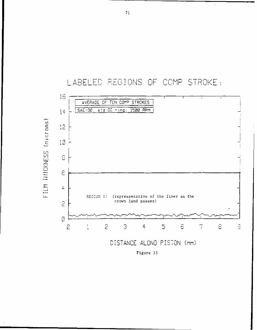
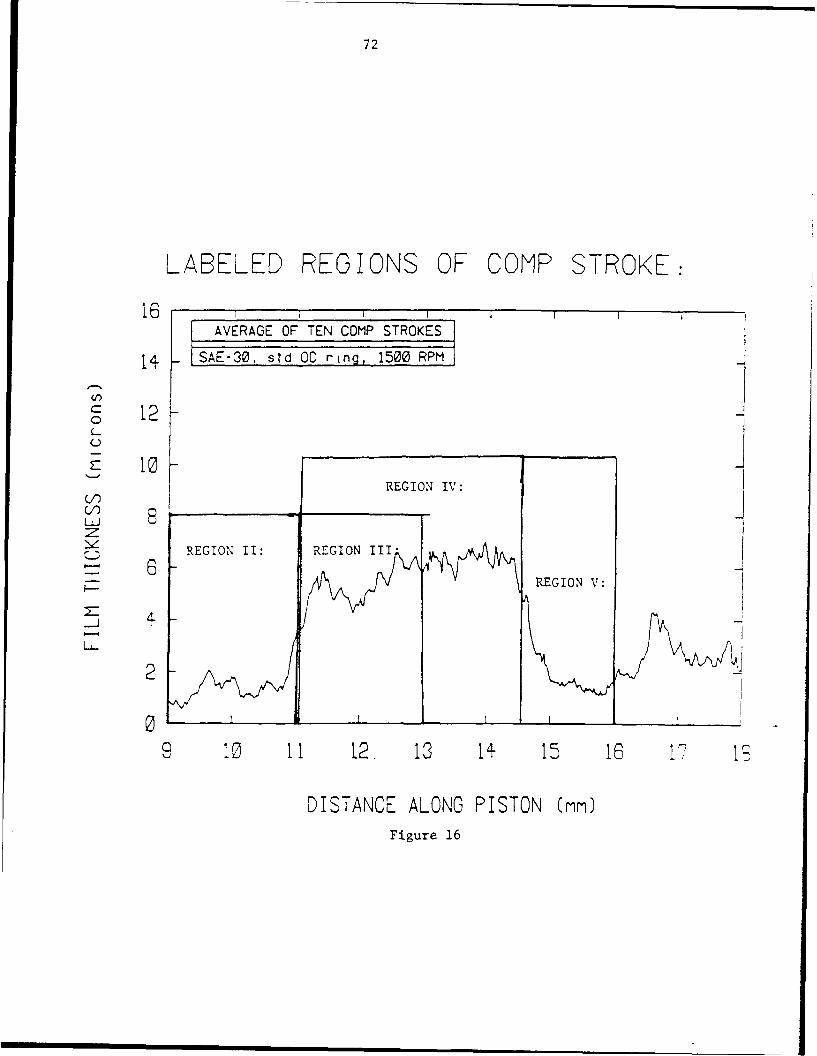
Figure 15. Labeled Regions of a Compression Stroke using SAE-30 and operatedat 1500 RPM at Full Load (0 mm to 9 mm along piston) ................ 71
Figure 16. Labeled Regions of a Compression Stroke using SAE-30 and operated
at 1500 RPM at Full Load (9 nn to 18 mm along piston) ............... 72
Figure 17. Oil Flow for the Power Exchange Strokes using SAE-30 ................. 73
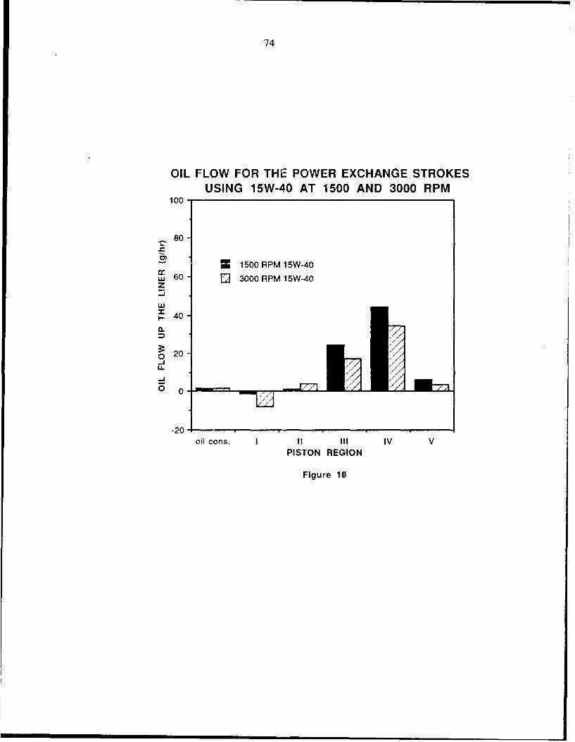
Figure 18. Oil Flow for the Power Exchange Strokes using 15W-40 ................. 74
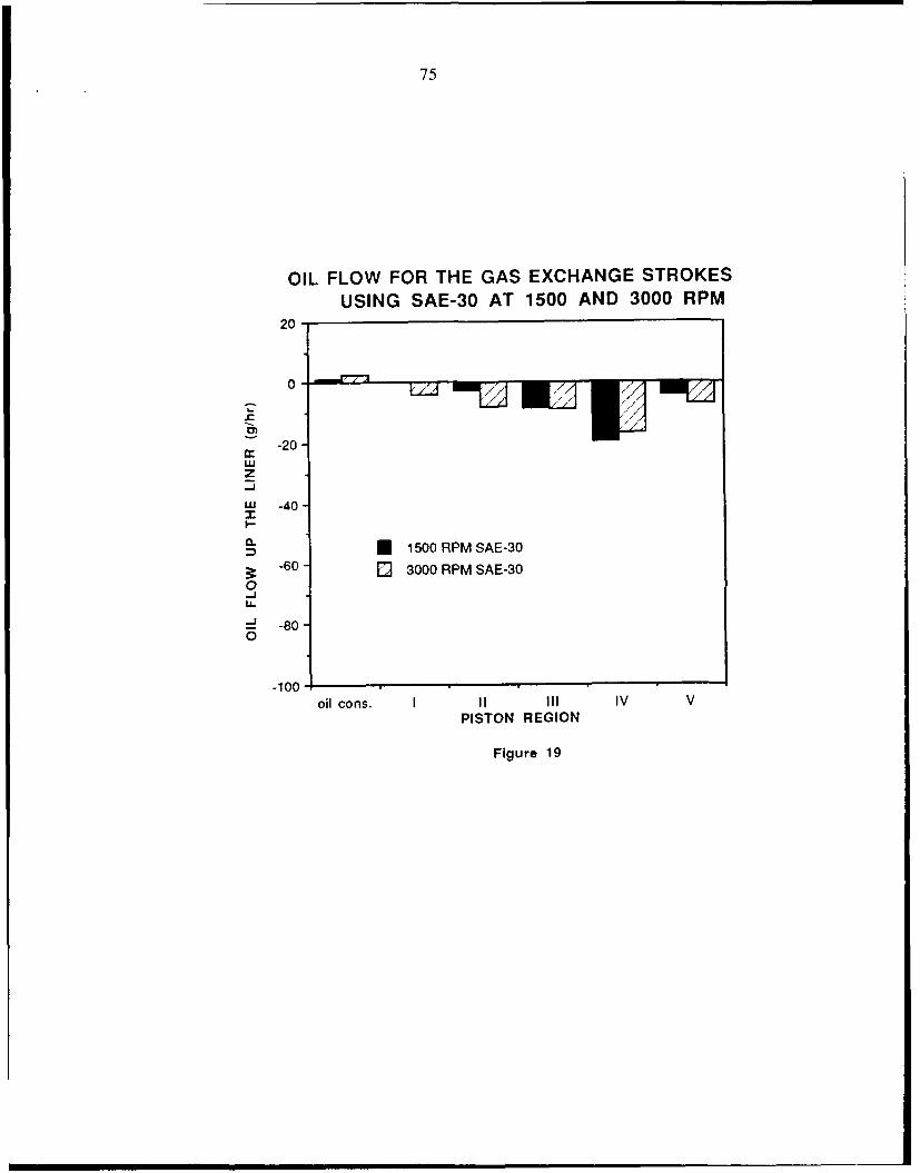
Figure 19. Oil Flow for the Gas Exchange Strokes using SAE-30 .................... 75
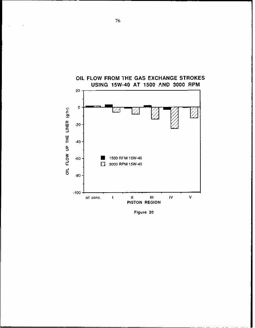
Figure 20, Oil Flow for the Gas Exchange Strokes using 15W-40 .................... 76
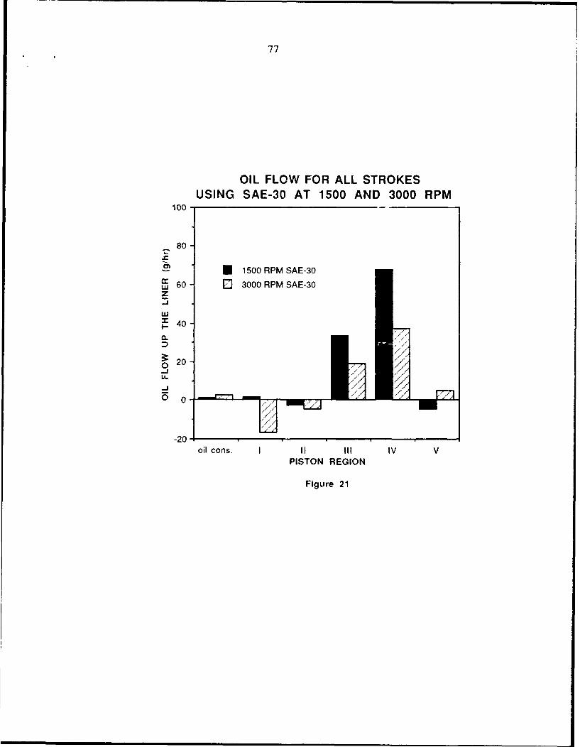
Figure 21. Oil Flow for all Strokes using SAE-30 ........................................ 77
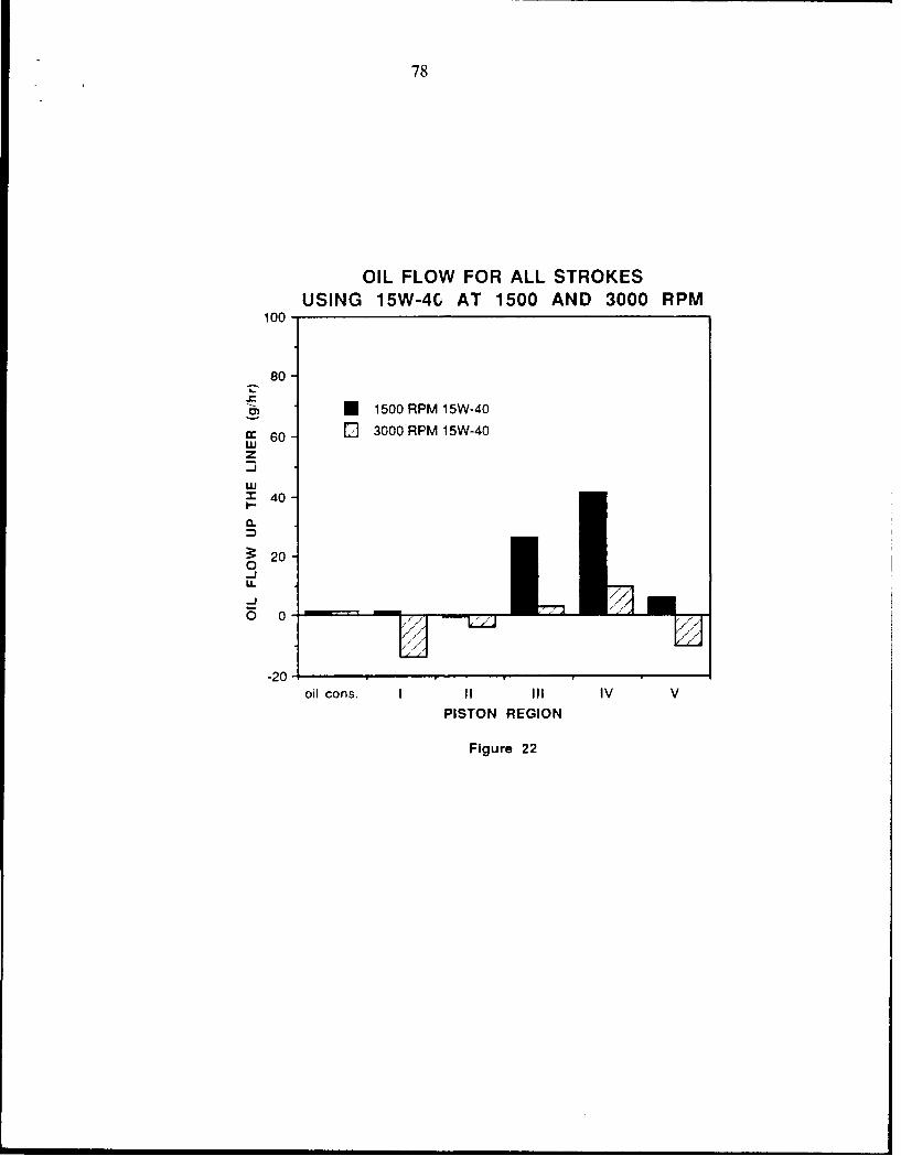
Figure 22. Oil Flow for all Strokes using 15W -40 ........................................ 78
9
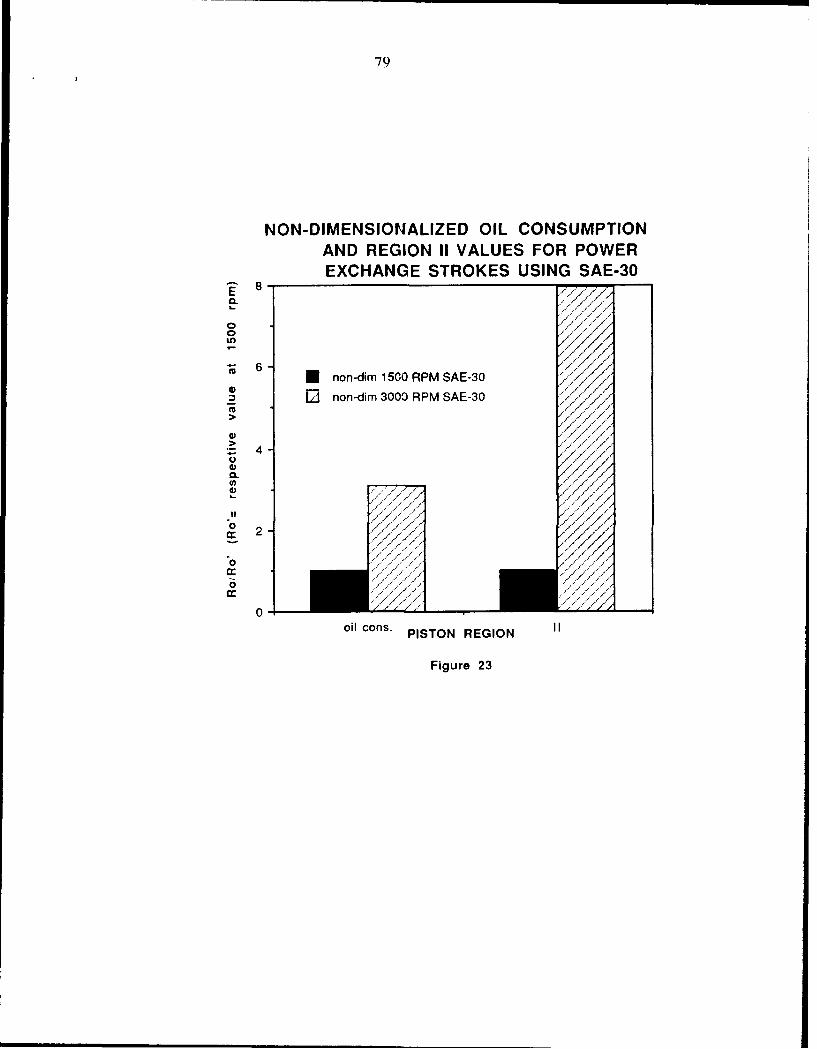
Figure 23. Non-dimensionalized Oil Consumption and Region II Values for thePower Exchange Strokes using SAE-30 .................................... 79
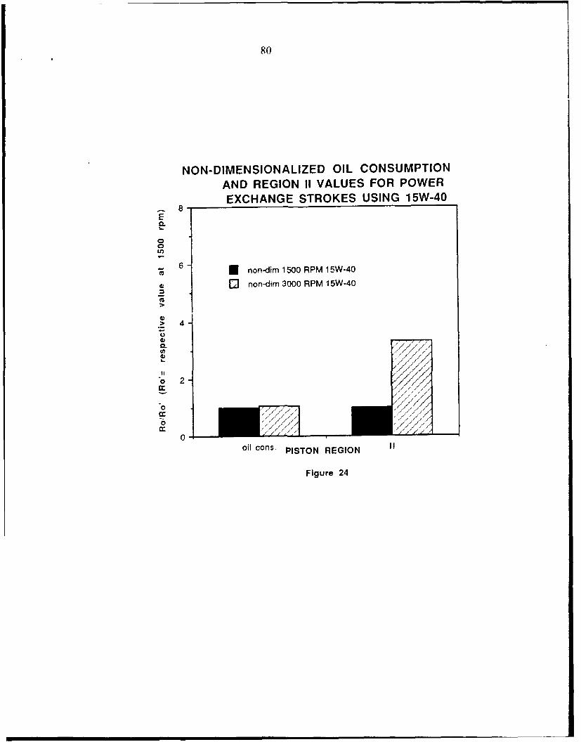
Figure 24. Non-dimensionalized Oil Consumption and Region II Values for thePower Exchange Strokes using 15W-40 ..................................... 80
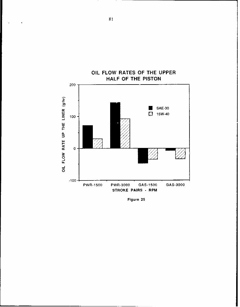
Figure 25. Oil flow rates for the upper half of the piston ................................ 81
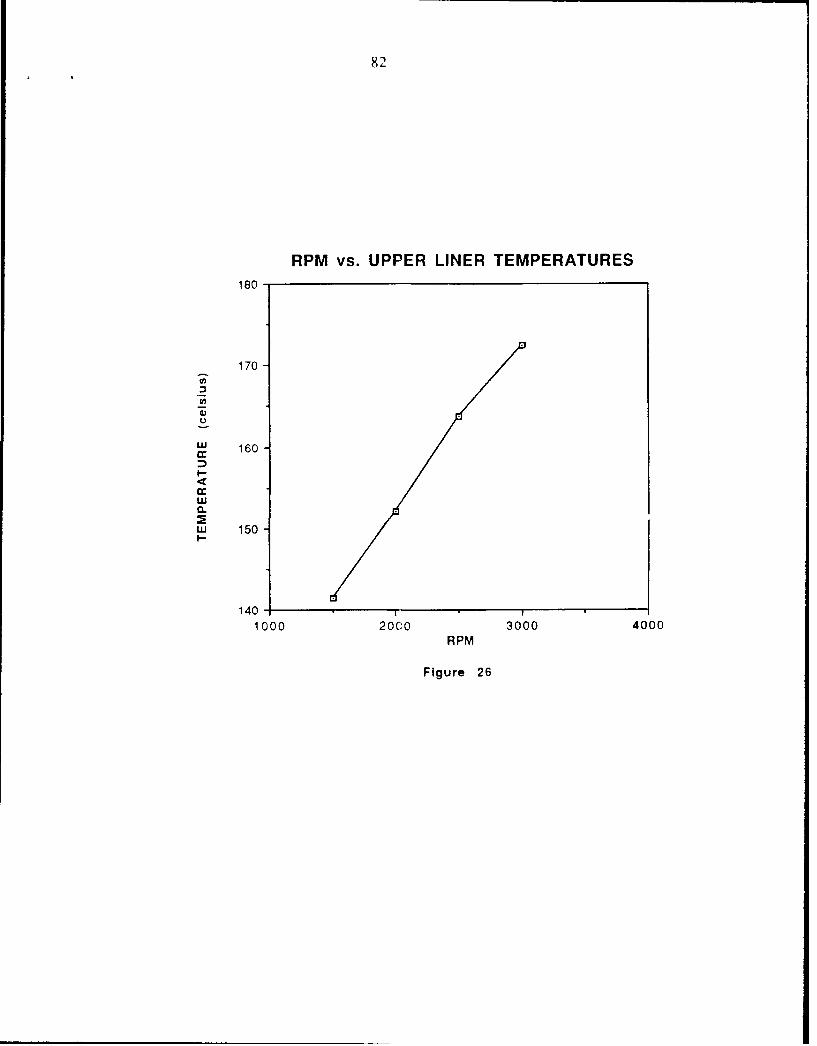
Figure 26. Tem perature vs. RPM .......................................................... 82
Figure 27. High and Low Shear viscosities vs. RPM .................................. 83
Figure 28. Surface Tension vs. RPM ..................................................... 84
Figure 29. Oil consumption vs. viscosities ............................................... 85
10
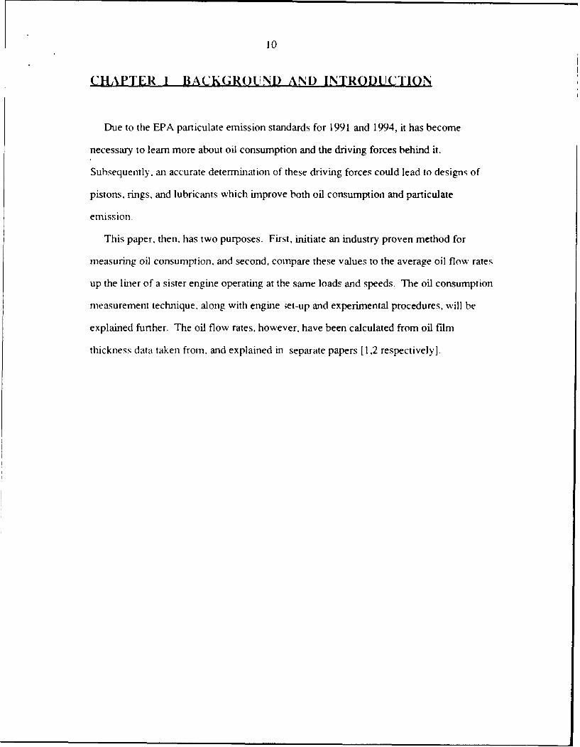
CHAPTER 1 BACKGROUND AND INTRODUCIION
Due to the EPA particulate emission standards for 1991 and 1994, it has become
necessary to learn more about oil consumption and the driving forces behind it.
Subsequently. an accurate detem-iination of these driving forces could lead to designs of
pistons, rings, and lubricants which inprove both oil consumption and particulate
emission.
This paper, then, has two purposes. First, initiate an industry proven method for
measuring oil consumption, and second, compare these values to the average oil flow rates
up the liner of a sister engine operating at the same loads and speeds. The oil consumption
measurement technique, along with engine ;et-up and experimental procedures, will be
explained further. The oil flow rates, however, have been calculated from oil film
thickness data taken from, and explained in separate papers [1,2 respectively].
11
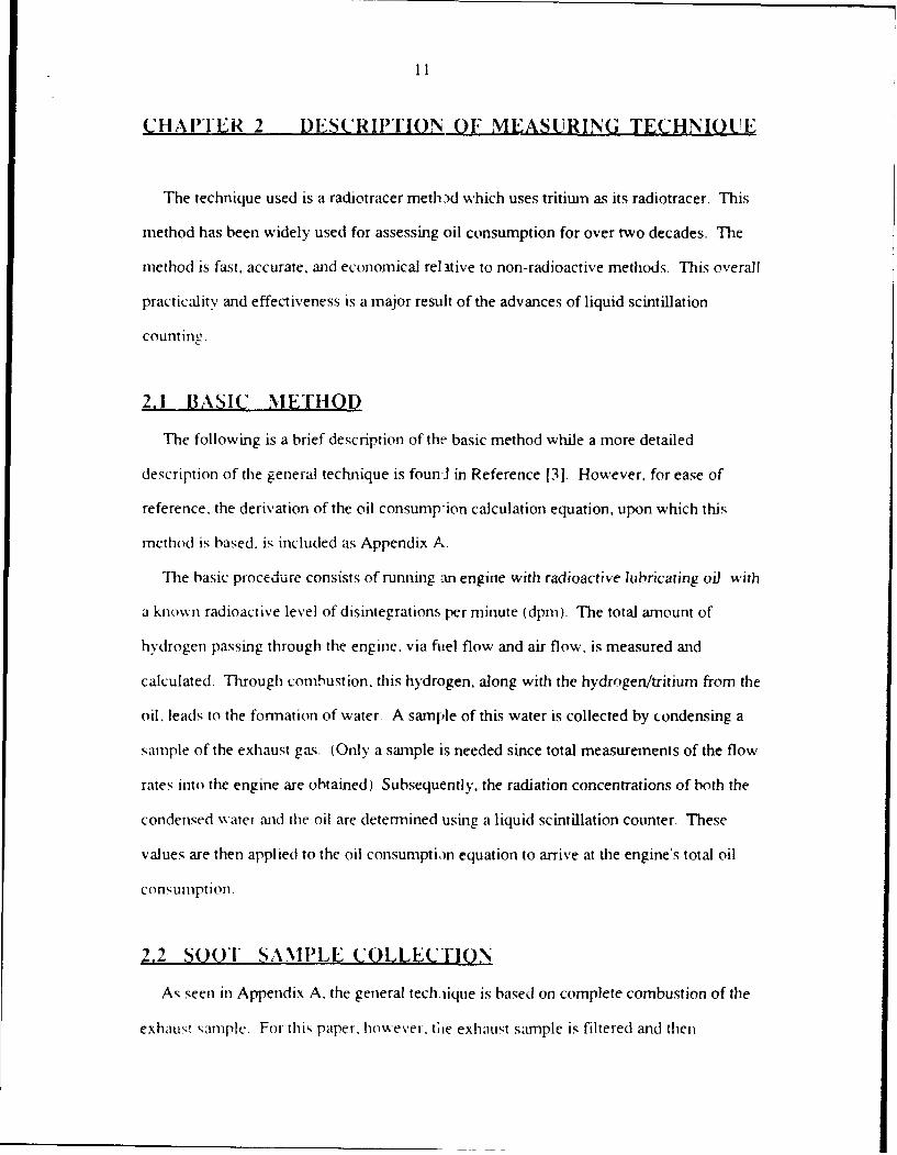
CHAPTER 2 DESCRIPTION OF MEASURING TECHNIOUE
The technique used is a radiotracer meth 3d which uses tritium as its radiotracer. This
method has been widely used for assessing oil consumption for over two decades. The
method is fast, accurate, and economical rel tive to non-radioactive methods. This overall
practicality and effectiveness is a major result of the advances of liquid scintillation
countingz.
2.1 BASIC METHOD
The following is a brief description of the basic method while a more detailed
description of the general technique is founI in Reference [3]. However. for ease of
reference, the derivation of the oil consumpion calculation equation, upon which this
method is based. is included as Appendix A.
The basic procedure consists of running -an engine with radioactive lubricating oil with
a known radioactive level of disintegrations per minute (dpm). The total amount of
hydrogen passing through the engine, via fuel flow and air flow, is measured and
calculated. Through combustion, this hydrogen, along with the hydrogen/tritium from the
oil, leads to the formation of water. A sample of this water is collected by condensing a
sample of the exhaust gas. (Only a sample is needed since total measurements of the flow
rates into the engine are obtained) Subsequently, the radiation concentrations of both the
condensed watet and the oil are determined using a liquid scintillation counter. These
values are then applied to the oil consumption equation to arrive at the engine's total oil
consuniption.
2.2 SOOT SAMPLE COLLECTION
As seen in Appendix A. the general tech.iique is based on complete combustion of the
exhaust smnple. For this, paper, howeveT. tiie exhaust sample is filtered and then

12
condensed instead of being completely combusted and then condensed. This results in an
activity concentration (dpmlml) of the condensed water and a total activity (dpm) of the soot
sample.
In order for this method to be valid, two assumptions are made. First, the soot
collected, if burned, would produce a negligible amount of water. Secondly, all of the
water vapor in the sample is being condensed. This latter assunption is necessary since the
consunption calculation requires radioactive concentrations vice total activities. Therefore.
the soot sample total activity is divided by the amount of water collected and then added to
the activity concentration of the water sample. A more in depth description of the
procedures is included in Appendix E.
2.3 LIOUID SCINTILLATION COUNTING [41
All radioactive levels are deternined by a method known as liquid scintillation counting.
This technique is highly sensitive and greatly responsible for the increased use of weak beta
emitters such as carbon-14 and tritium. The basic technique, as with other methods of
measuring radioactivity, relies on the interaction of nuclear radiation with matter. In this
case, a luminescent material, or scintillator, is excited by radioactive disintegrations.
A scintillator. also referred to as either a phosphor or sometimes a fluor, is defined as a
material which emits a brief pulse of fluorescent light when interacting with a high-energy
particle or quantum. Therefore, the radioactive samples used in this experiment are mixed
with a scintillator. The subsequent flashes of light, or scintillations, are detected by the
co'rnter by use of a photomultiplier. This in turn, over a set period of time, allows for the
detennination of the average disintegrations per minute (dpm) of each sample.
13
CHAPTER 3 EOUIPMENT AND SET-UP
3.1 ENGINE
The engine used in this experiment is the KUBOTA EA300N, a single cylinder,4-
stroke, IDI diesel. This engine is used prinarily for remote power generation. A detailed
description of the engine's geometry and performance is included in Appendix B.
This engine was chosen only because the film thickness measurements used in this
paper were obtained from an engine of the same make and model [1 ].
3.2 RADIOACTIVE LUBRICATING OILS
Radioactive oil for these experiments is purchased commercially. The oil received has
been through a tritiation process which results in approximately 250 mCu in one ml of oil.
Subsequently. this oil is divided up and thoroughly mixed with Pennzoil SAE-30 (single-
grade) and Pennzoil 15W-40 (multi-grade). The tritiation process is explained further in
AppendLix B.
These oils are used prinarily for the same reason as above for the engine. In addition,
they should provide a good comparison of single- and multi-grade oils since the only
difference is the addition of a polymer VI improver to the 15W-40.[31
3.3 ENGINE INSTRUMENTATION
The engine is fitted with thernocouples 'n order to monitor operating temperatures (Fig.
1). The thennocouples measure the inlet air temperature, the coolant temperature, the oil
sump temperature, the exhaust temperature, and the liner temperatures. The latter
thermocouples coincide with the top ring at TDC. mid-stroke, and BDC. A laminar air
flow element is also used to measure the air flow while a burette system is used to measure
the volume flow rate of the fuel. A more detailed listing of the measuring equipment is
included in Appendix B.
14
3.4 DESCRIPTION OF PISTON AND RINGS 121
The piston and rings (Fig. 2) are represtntative of modem engine design. The piston is
made of aluminum and accommodate three piston rings. It has round lands and a barrel
shaped skirt. Behind and below the oil control ring, there are oil flow relief holes that
allow the circulation of oil up the piston skirt on the liner side and back down to the sump
inside the piston.
The three piston rings consist of a top ring, a scraper ring, and an oil control ring. The
top ring is a half-keystone design with a 70 keystone angle. It is made out of cast iron with
a chromium strip embedded into its face to improve wear resistance. The resulting face
profile is asynunetric. The scraper ring has a tapered face and an undercut on its face side
to provide the correct tilt angle when compiessed to its working diameter. It is also made
of cast iron. The oil control ring is a one piece type made of cast iron also, and, like the top
ring, its rails have a chromium strip embedded into them. The oil control ring also has
slots between the rails to allow the flow of oil through the ring to the holes in the piston
mentioned above.
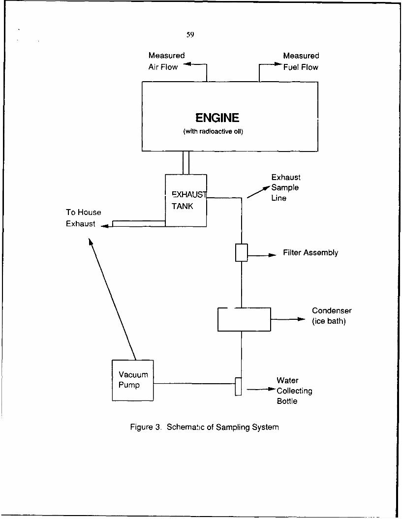
3.5 SAMPLING SYSTEM
Figure 3 is a schematic of the sampling system in use. As shown, the sampling system
is connected to an exhaust tank. This tank is used to help eliminate the exhaust pulse that
exists when operating a single cylinder eng;ne. This entire system, consisting of
inexpensive components, is placed on a small lab cart which allows for portability and for
an easy connection to a different engine.
15
3.6 OIL FILM THICKNESS MEASUREMENTS
The filn thickness traces referred to are obtained from reference [I] which uses a laser-
fluorescence technique. This basic techniqLe consists of mixing the lubricant with a
fluorescent dye and then, during operation, focusing a HeCd (blue) laser through a quartz
window installed in the liner. The resulting fluoresced (green) light is then collected and
converted to a voltage signal using a photomultiplier [2]. Lastly, the voltage signal is
converted into microns using a calibration coeffecient (unique for each trace). This
coeffecient is based on the voltage readings obtained when etch marks of known depths on
the piston skirt pass the quartz window.[1]
More in depth descriptions of this technique can be found in references [1] and [2].
16
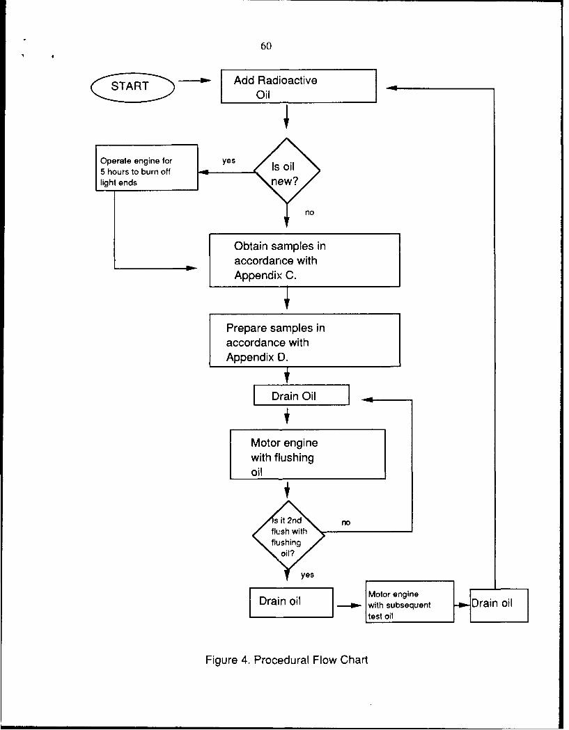
CHAPTER 4 DESCRIPTION OF EXPERIMENTS
4.1 PROCEDURES
At each given load and speed, the engine is allowed to stabilize. Subsequently, flow
rates are measured and samples are taken in accordance with the step-by-step procedures in
Appendix C. The samples are then prepared in accordance with Appendix D in order for
the scintillation counter to be effective.
Following sample preparation, the samples are placed in the scintillation counter to
determine their individual radioactive levels. These values, along with the measured flow
rates, are then used to calculate oil consumption. Actual formulas and an example of the
spreadsheets in use are included in Appendix E.
After collecting data using the first oil, the engine is flushed to minimize contamination
of the next test oil. A flow chart of these basic procedures is illustrated in figure 4.
4.2 ENGINE OPERATING CONDITIONS
The primary loading conditions for each oil consisted of full load at 1500 rpm and
full load at 3000 rpm (approximately 9.5 ft-lbs for each). As before, these conditions were
used in order to duplicate the conditions under which the film thickness data was taken.
Secondary loading conditions consisted of 2000 rpm and 2500 rpm at the same torque.
These latter conditions were used mainly fcr graphic continuity between low and high
speeds.
17
CHAPTER 5 GRAPHIC RESULTS
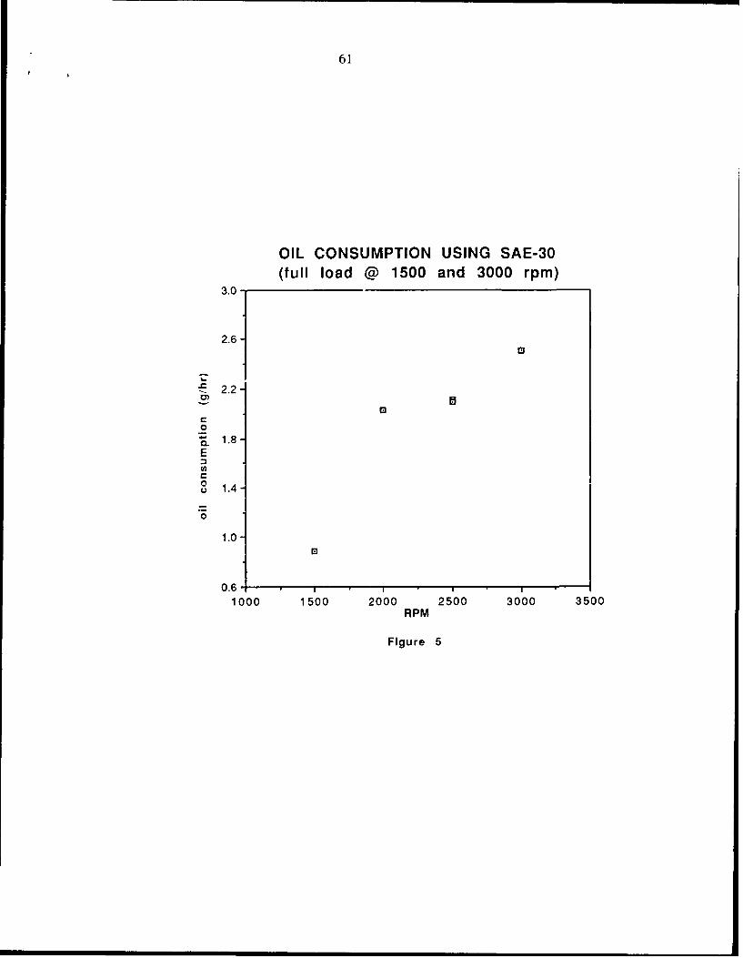
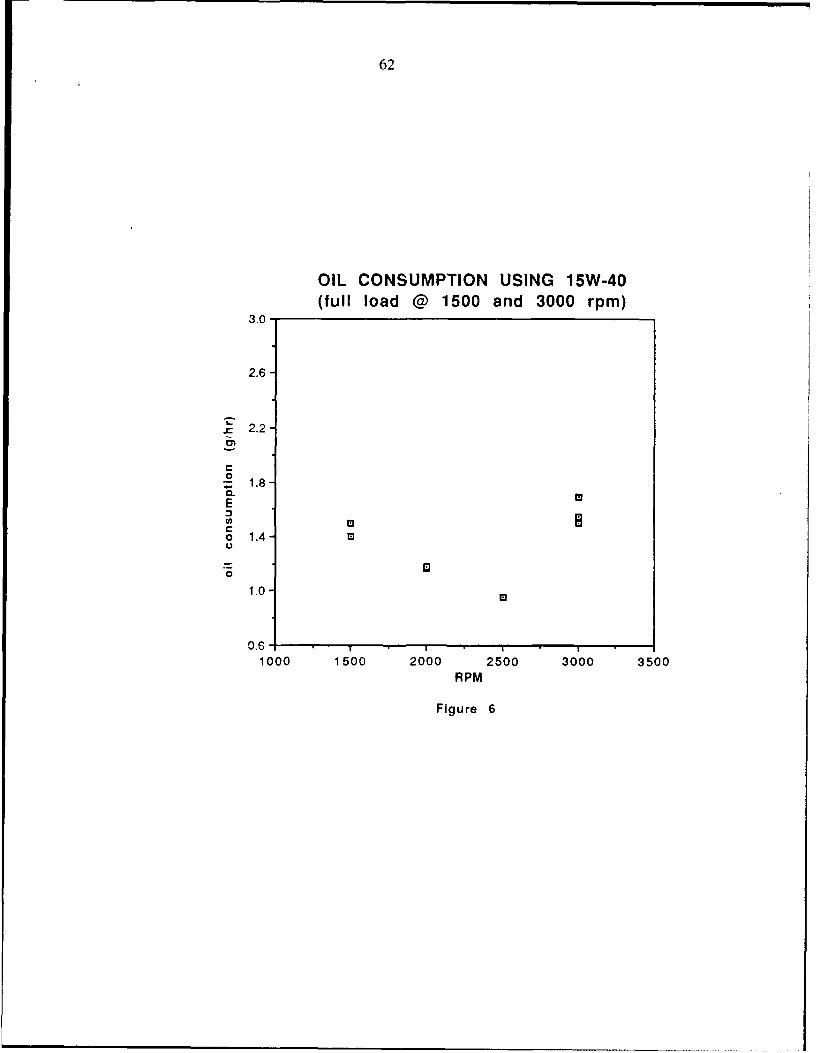
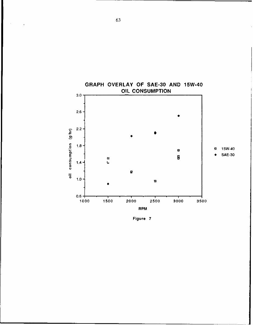
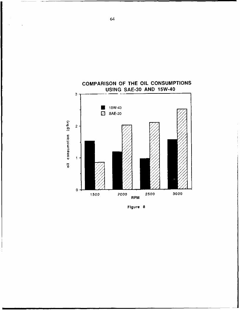
5.1 OIL CONSUMPTION MEASUREMENTS
Oil consumption measurements for the desired load and speeds using Pennzoil's SAE-
30 and 15W-40 are illustrated in figures 5 and 6, respectively. Figure 7 is then an overlay
of the previous two graphs with figure 8 being another comparison but in the form of a bar
chart.
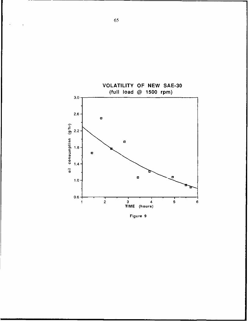
The volatility of a new oil (SAE-30) is also examined. The results, included as figure 9,
illustrate how oil consumption rates decrease and then stabilize with time (for a constant
load and speed). Volatilit- information is (desirable since the film thicknesses were
obtained from the sister Kubota using new lubricating oils.
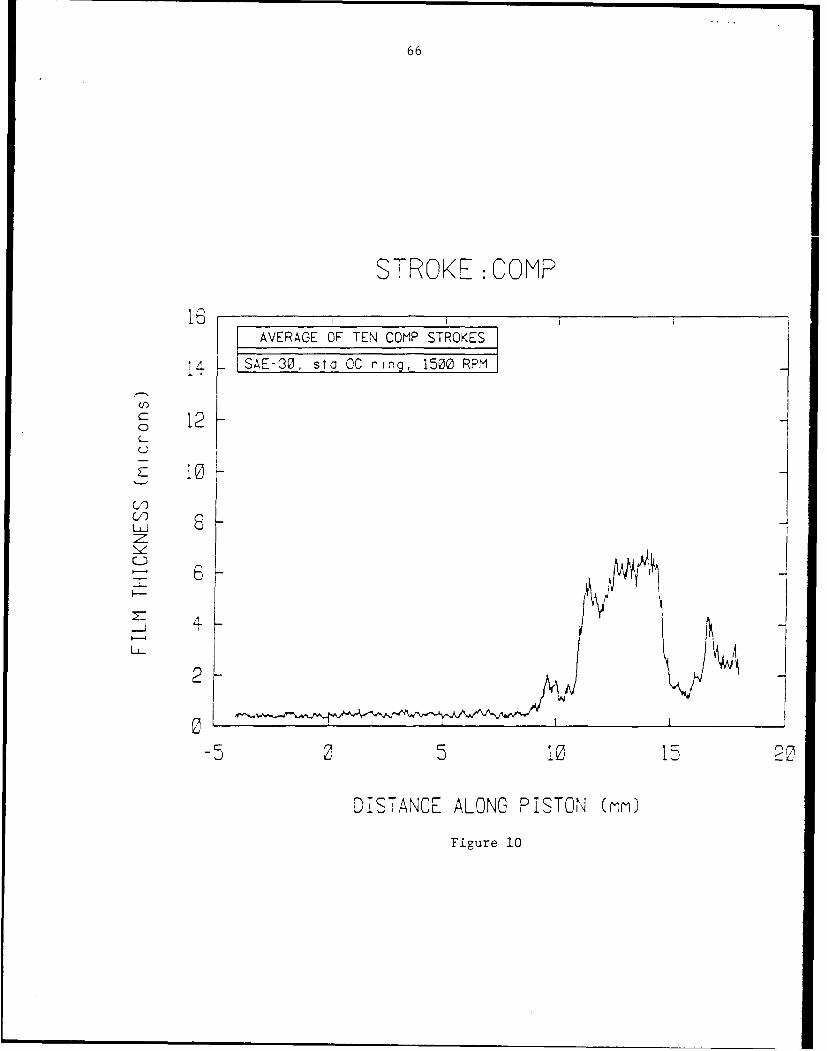
5.2 OIL FILM THICKNESSES
Figures 10. 11, 12, and 13 illustrate a subset of the average film thickness traces for ten
compression, expansion, exhaust, and intake strokes, respectively [1]. For these traces,
the engine was using SAE-30 and was running at full load at 1500 rpm. The traces for
3000 rpm and for the different oil are similar to these and are therefore not included.
Interpretation of this data, which can be confusing to the first-time observer, is described in
length in reference [2].
18
CHAPTER 6 ANALYSIS AND DISCUSSION
6.1 HYPOTHESES
There exists three prevalent hypotheses on lubricating oil consumption, two of which
deal with oil being drawn in and around the top ring at or near the end of the expansion
stroke. At this point, the high pressure below the top ring forces the oil around the top ring
where it either (1) accumulates on the crown land from where it is later burned off or (2) is
"blown" up into the combustion chamber and consumed. The third hypothesis is based on
oil being transported by the top ring face. Subsequently, some of this oil is deposited onto
the liner at or near top ring reversal (TRR) where it is later consumed.
For each hypothesis, there exists a corresponding volume. These volumes are
calculated by first finding their respective aeas which are illustrated in figure 14. The areas
are then swept around the circumference of the bore to determine the volumes. Table 1 lists
the areas and the volumnes calculated.
SPACE AREA (mm 2 ) VOLUME (mmun 3)
A) Crown land crevice 1.33 313.0
B) Ring/groove crevice 0.3 70.7
(top and bottom)
C) Ring/groove crevice 1.02 241.0
(backside of ring)
D) Between ring and liner .00386 0.91
Table 1. Areas/Volumes of possible oil consumption mechanisms
19
These volumes can in turn be related to an oil flow rate, in g/hr, based on engine
operating speed and oil density (Refer back to Appendix E). Unfortunately, volumes A, B,
and C above result in rates on the order of thousands of grams per hour with volume D
being on the order of 50 grams per hour. These values are extraordinarily high and do
not scale with oil consumption (figures 5 ard 6). Thus they cannot offer much guidance in
determining oil consumption mechanisms. Actual volumes necessary to resemble the oil
consumption values are on the order of 0.01% of volumes A and C, 0.05% of volume B,
and Just 3.0% of volume D.
6.2 ANALYSIS AND DISCUSSION
As discussed in Chapter 5 of reference [2], the film thickness data does not usually
allow for a determination of where the oil lies (i.e. on the piston, on the liner, or on both).
However, as figures 10 through 13 illustrate, the oil film thickness before the piston arrives
(-4mam to 0mm for the upstrokes) is relatively the same as when the crown land is passing
(0rn to 9.5nm for the upstrokes). Therefore, it is apparent that the piston crown land is
virtually oil free and thus, does not contribute to oil consumption. It is important to
mention that this film trace characteristic is also shared by the other traces for the higher
speed and with the different oil.
Based on the above line of reasoning, the first hypothesis can be easily refuted. The
second one, however, can neither be directly refuted nor explicitly proved by this method
of film measurement. This is because the hypothesis addresses oil which enters the
combustion chamber by way of neither the piston nor the liner. However, further data
analysis of the film traces does allow for some broad conclusions to be made concerning
both this and the final hypothesis.
This subsequent data analysis first requLes the use of existing computer programs
which have been modified for the Kubota eilgine [5]. These programs calculate the volume
differences (mm 3/cycle) of various crank angle regions for both the power and the gas
20
exchange strokes. Only five regions, which are listed below in Table 2, are analyzed in
this paper. The methods and reasons for computing these particular regions, along with
copies of the programs, are included in Appendix F.
REGION PISTON AREA
I Crown land
II Top Ring
III 1 ring width below top ring
IV Second Land
V Second (Scraper) Ring
Table 2. Piston Regions of Film Thickness
The title of each region in the table explains which part of the piston is passing the
quartz window at that instant. In addition, the regions are labeled on an expanded version
of the aforementioned compression stroke. (Figures 15 and 16)
Secondly, in order to compare a regions volume difference to the measured oil
consumption, the former is converted to an oil flow rate up (or down) the liner in g/hr.
This is done based on the volume difference, the speed, and the oil's density. (Refer back
to Appendix E for calculations)
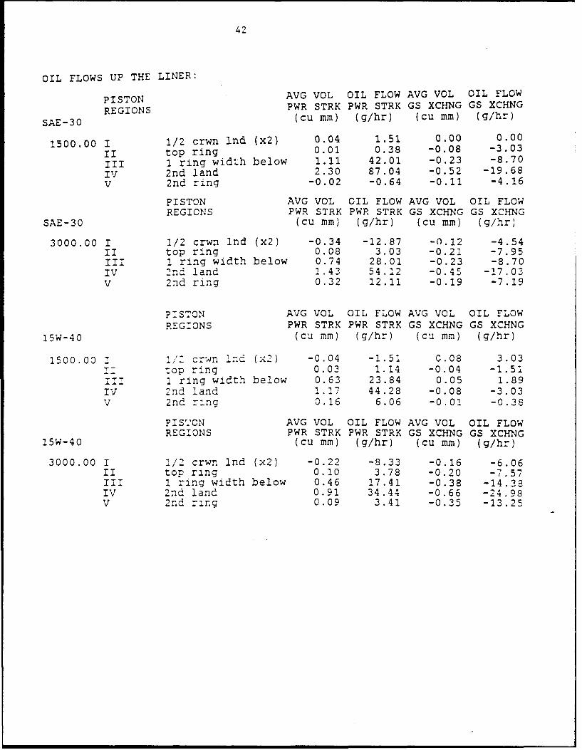
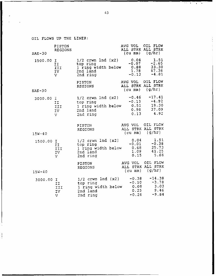
Tables 3 and 4 and Tables 5 and 6 tabulate the data collected using SAE-30 and 15W-
40, respectively. A positive value indicates that the upstroke volume is greater than the
downstroke and vice versa. Subsequently, figures 17 through 22 are included to illustrate
these various flow rates of the two oils for the different speeds. On each figure, the
respective oil consumption is included in order to make relative comparisons.
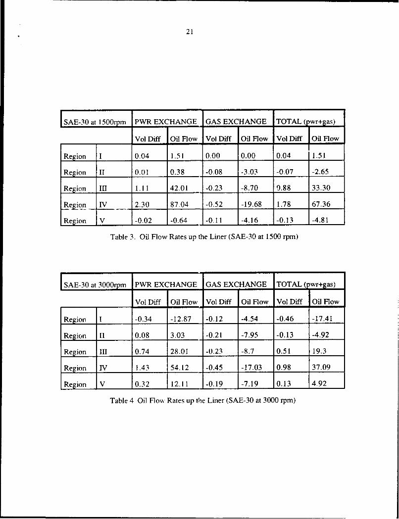
21
SAE-30 at 1500r m PWR EXCHANGE GAS EXCHANGE TOTAL (pwr+gas)
Vol Diff Oil Flow Vol Diff I Oil Flow Vol Diff I Oil Flow
Region I 0.04 1.51 0.00 0.00 0.04 1.51
Region II 0.01 0.38 -0.08 -3.03 -0.07 -2.65
Region III 1.11 42.01 -0.23 -8.70 9.88 33.30
Region IV 2.30 87.04 -0.52 -19.68 1.78 67.36
Region V -0.02 -0.64 -0.11 -4.16 -0.13 -4.81
Table 3. Oil Flow Rates up the Liner (SAE-30 at 1500 rpm)
SAE-30 at 3000rpm PWR EXCHANGE GAS EXCHANGE TOTAL (pwr+gas)
Vol Diff Oil Flow Vol Diff Oil Flow Vol Diff Oil Flow
Region I -0.34 -12.87 -0.12 -4.54 -0.46 -17.41
Region II 0.08 3.03 -0.21 -7.95 -0.13 -4.92
Region III 0.74 28.01 -0.23 -8.7 0.51 19.3
Region IV 1.43 54.12 -0.45 -17.03 0.98 37.09
Region V 0.32 12.11 -0.19 -7.19 0.13 4.92
Table 4 Oil Flow Rates up the Liner (SAE-30 at 3000 rpm)
22
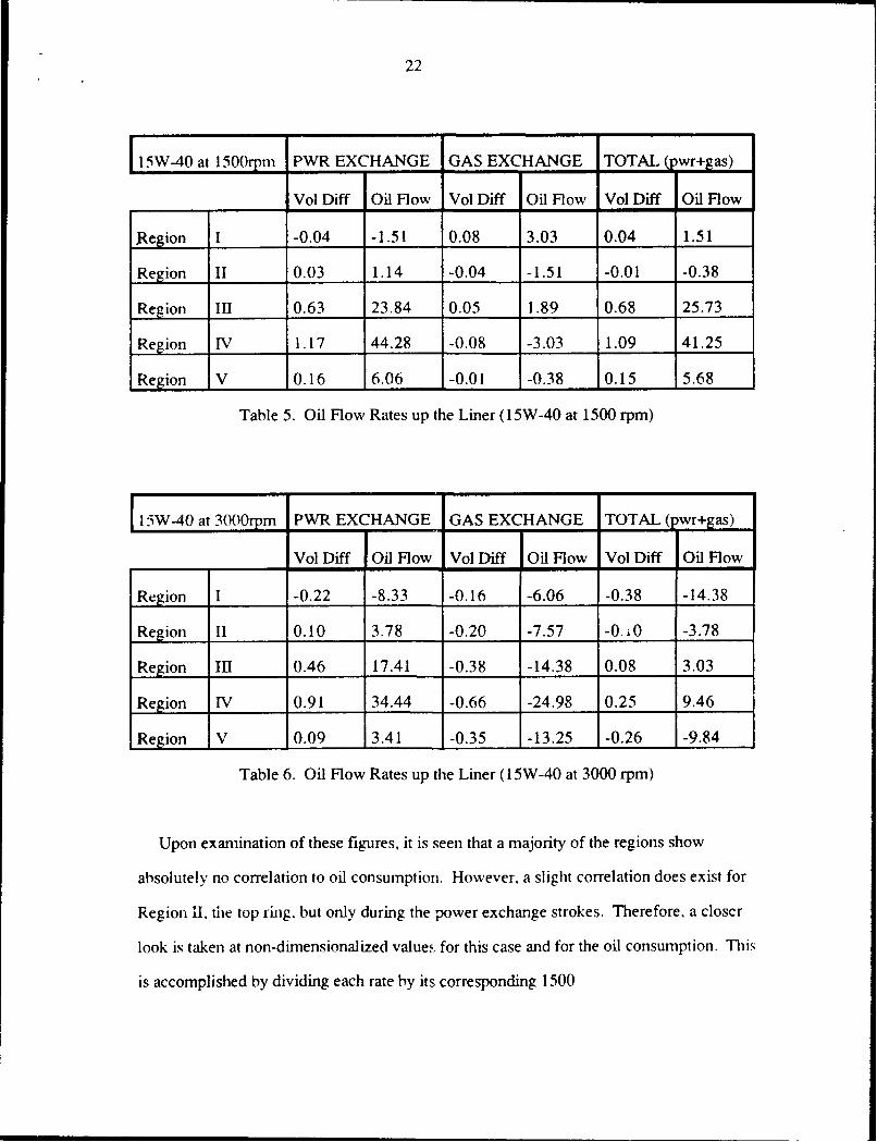
115W-40at1500rm PWR EXCHANGE GAS EXCHANGE TOTAL (wr+gas)
Vol Diff Oil Flow VolDiff Oil Flow VolDiff Oil Flow
,Region I -0.04 -1.51 0.08 3.03 0.04 1.51
Region II 0.03 1.14 -0.04 -1.51 -0.01 -0.38
Region I11 0.63 23.84 0.05 1.89 0.68 25.73
Region IV 1.17 44.28 -0.08 -3.03 1.09 41.25
Region V 0.16 6.06 -0.01 -0.38 0.15 5.68
Table 5. Oil Flow Rates up the Liner (15W-40 at 1500 rpm)
11lW-40at300m PWR EXCHANGE GAS EXCHANGE TOTAL (pwr+gas)
Vol Diff Oil Flow Vol Diff Oil Flow Vol Diff Oil Flow
Region I -0.22 -8.33 -0.16 -6.06 -0.38 -14.38
Region II 0.10 3.78 -0.20 -7.57 -0.i0 -3.78
Region III 0.46 17.41 -0.38 -14.38 0.08 3.03
Region IV 0.91 34.44 -0.66 -24.98 0.25 9.46
Region V 0.09 3.41 -0.35 -13.25 -0.26 -9.84
Table 6. Oil Flow Rates up the Liner (1 5W-40 at 3000 rpm)
Upon examination of these figures, it is seen that a majority of the regions show
absolutely no correlation to oil consumption. However, a slight correlation does exist for
Region ii, the top ring, but only during the power exchange strokes. Therefore, a closer
look is taken at non-dimensionalized values for this case and for the oil consumption. This
is accomplished by dividing each rate by its corresponding 1500
23
rpm value. (i.e. all of the 1500 rpm values will equal one) The results are illustrated in
figure 23 for SAE-30 and figure 24 for 15W-40, however, it is seen that the oil flow rates
do not duplicate the trends of the oil consumption in either case.
6.3 PROBABLE ERRORS IN ANALYSIS TECHNIQUE
When comparing oil flow rates to oil consumptions, if in fact fdm thickness in this case
can even be related to oil consumption, only trends can be looked for. An exact matching
of values would be virtually impossible for the following reasons:
a) Oil consumption measurements vary within an engine, therefore they willvary even more between separate, but identical, engines.
b) The oil film data is obtained while using new, and thus more volatile,lubricating oil. (Refer back to figure 9)
c) As previously mentioned, the calibration coefficients for each film trace aredetermined by way of etch marks on the skirt [1]. However, there mayexist a temperature gradient between the skirt and the rings and lands.This gradient would result in different calibrations for these latterregions since the fluorescence of the oil is inversely proportional to itstemperature [6].
d) The oil flow relief holes, described in sect.3.4, is probably what attributesto the absence of correlation between oil consumption and film thickness.Figure 25 illustrates that, over the length of the piston, the power strokestend to have more oil on the way up then on the way down and vice versafor the gas exchange strokes. These results imply that:
1 ) after the oil control ring passes the window on the compressionstroke and before it passes the window on the expansion stroke, oilis returned to the sump via the flow holes.
2) after the oil control ring passes the window on the exhauststroke and before it passes the window on the intake stroke, oilis supplied to the sump via the flow holes.
24
6.4 MISCELLANEOUS ANALYSIS
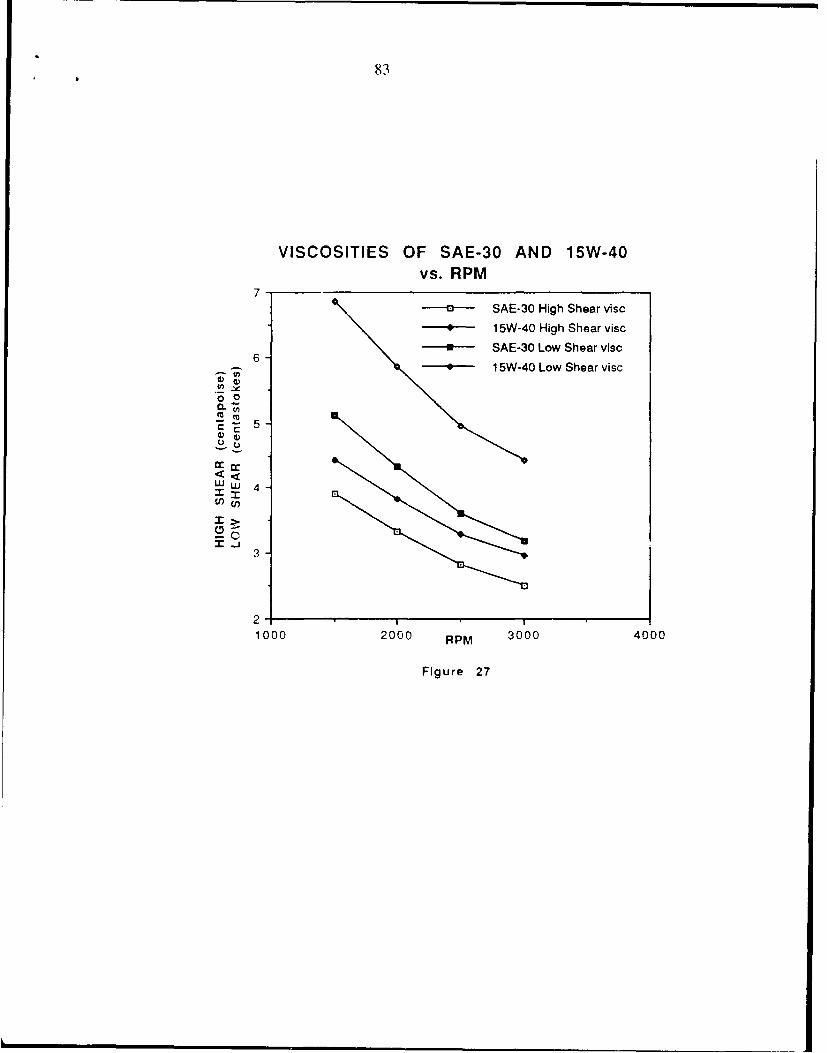
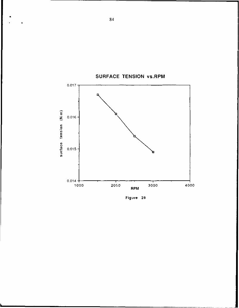
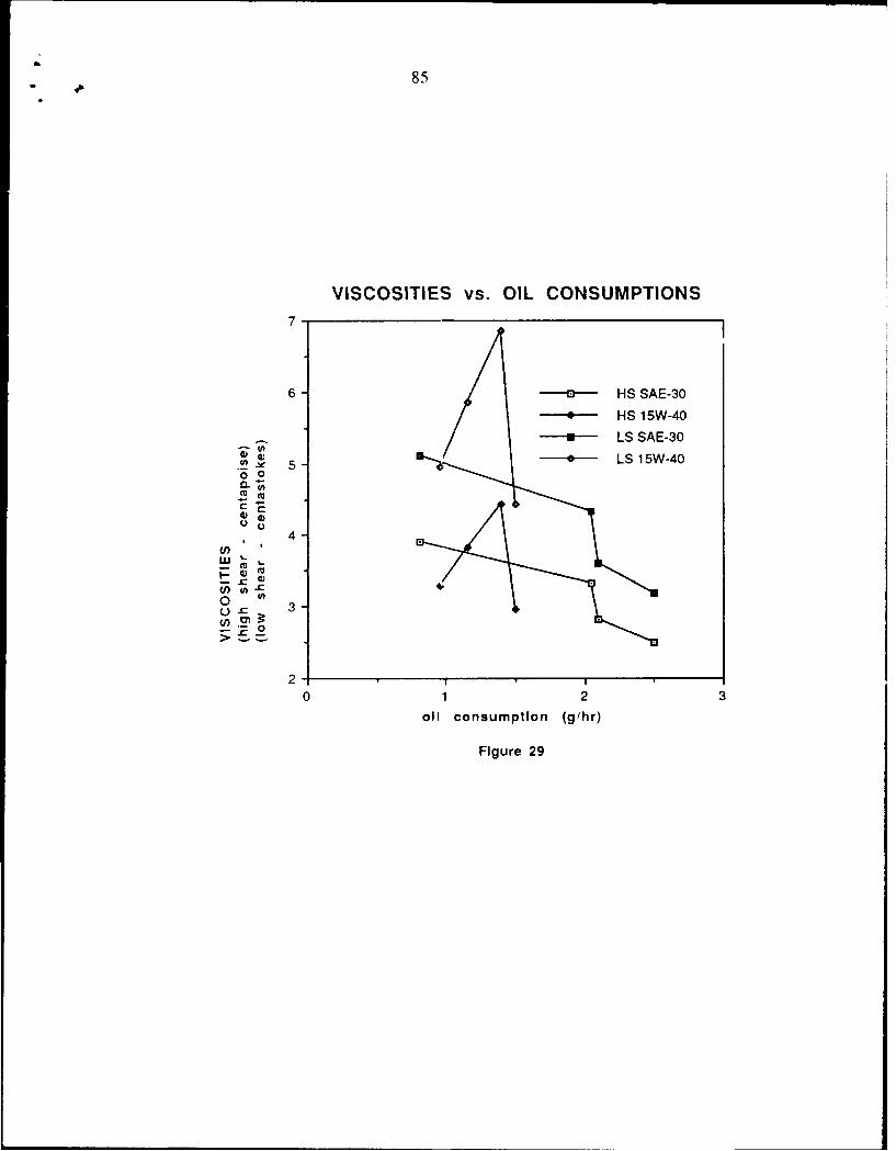
The temperature of the upper portion of the liner during operation is plotted in figure 26
for the RPMs shown. These temperatures are then used to determine the high and low
shear viscosities (figure 27) and the surface tension (figure 28) of the oils in
use [7]. Lastly, the oil consumptions versus viscosities are plotted in figure 29.
Unfortunately, no trends or relationships between the two are observed.
25
CHAPTER 7 CONCLUSIONS AND RECOMMENDATIONS
The primary conclusions and recormmendations are as follows:
1) The crown land is virtually dry' and therefore does not contribute to oil
consumption.
2) The top ring is the only region whose oil film thickness characteristics remotely
resemble oil consumption. llowcver. before any conclusions can be fonnulated, more
comparisons need to be made between this region's flow rate and oil consumption.
3) The concept of oil being "blown' around the top ring and into the combustion
chamber is still a viable solution, however. :he top ring region might be an additional
driving force behind oil consumption.
4) The oil flow relief holes provide a significant unknown which might make this
type of flow rate analysis for this particular set-up invalid. A recommended set-up would
consist of obtaining film thickness measuretments through a window placed such that the oil
control ring never passes over it.
26
REFERENCES
1. Bliven, M., "Oil Film Measurements for Various Piston Ring Configurations in aProduction Diesel Engine", S.M. Thesis, Massachusetts Institute of Technology,Department of Ocean Engineering, 1990.
3. Warrick, F. and Dykehouse. R., "An Advanced Radiotracer Technique forAssessing and Plotting Oil Consumption in Diesel and Gasoline Engines",SAE Paper #700052, 1970.
2. McElwee, M., "Comparison of Single-grade and Multi-grade Lubricants in aProduction Diesel Engine", S.M. Thesis, Massachusetts Institute of Technology,Department of Mechanical Engineering, 1990
4. Schram, E., Organic Scintillation Detectors, Elsevier Publishing Company, 1963.
5. Lux, J., "Lubricant Film Thickness Measurements in a Diesel Engine",S.M. Thesis.Massachusetts Institute cr fechnology, Department of MechanicalEngineering. 1989.
see also: Lux, Hoult, Olechowski, "Lubricant Film Thickness Measurementsin a Diesel Engine Piston Ring Zone", STLE Annual Mtg, Denver, ColoradoMay 7-10, 1990.
6. Takiguchi, M. and Hoult, D., "Calibration of the Laser Fluorescence TechniqueCompared with Quantum Theory", ASME - STLE Tribology Conference, Toronto,Canada, October 7-10, 1990.
7. Olechowski, M., "Analysis of Single and Multi-grade Lubricant Film Thickness in aDiesel Engine", S.M. Thesis, Massachusetts Institute of Technology,Department of Mechanical Engineering, 1990
8. Law, D. New England Nuclear, personal communication March 1990.
9. "Radiotracer Procedures", Sealed Power Corporation, 1988.
10. Hass. A. Internal Correspondence, Sealed Power Corporation. 1988.
11. Manual for Meriam Laminar Flow Elements, Meriam Instruments.
12. Heywood. J.B., Internal Combustion Engine Fundanentals. McGraw-Hill. 1988.p.12.
27
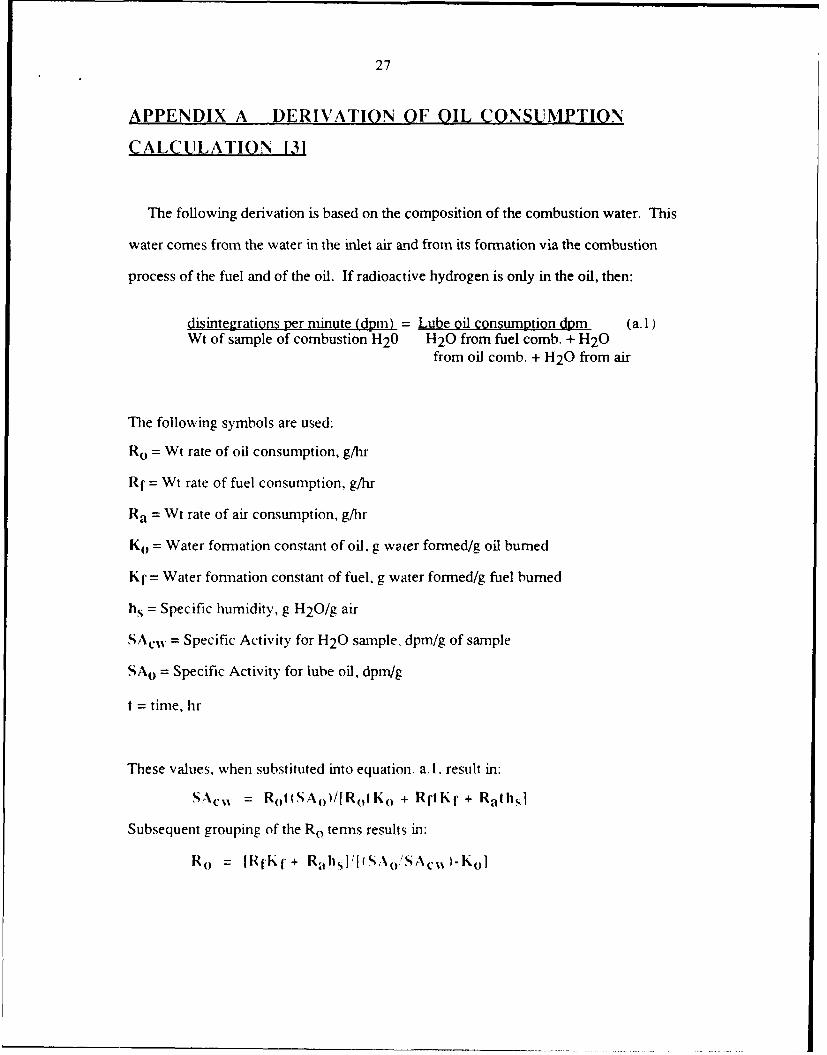
APPENDIX A DERIVATION OF OIL CONSUMPTION
CALCULATION 131
The following derivation is based on the composition of the combustion water. This
water comes from the water in the inlet air and from its formation via the combustion
process of the fuel and of the oil. If radioactive hydrogen is only in the oil, then:
disintegrations per minute (dpm) = Lube oil consumption dtpm (a. 1)Wt of sample of combustion H2 0 H2 0 from fuel comb. + H2 0
from oil comb. + H2 0 from air
The following symbols are used:
Ro = Wt rate of oil consumption, g/hr
Rf = Wt rate of fuel consumption, g/hr
Ra = Wt rate of air consumption, g/hr
Ko = Water formation constant of oil, g water formed/g oil burned
Kf= Water formation constant of fuel. g water formed/g fuel bumed
hs = Specific humidity, g H20/g air
SAc(N = Specific Activity for H2 0 samnple, dpm/g of sample
SA O = Specific Activity for lube oil, dpnVg
I = time, hr
These values, when substituted into equation. a. 1. result in:
SAcjN = RoIt(SAO)/[Ro K o + RfI Kf + Rahs
Subsequent grouping of the Ro tenns results in:
R o = [RI.K f + R 1 hsj,,'SAo/SAcN )-K o]
28
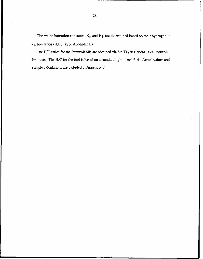
The water formation constants, Ko and Kf, are determined based on their hydrogen to
carbon ratios (H/C). (See Appendix E)
The H/C ratios for the Pennzoil oils are obtained via Dr. Tayeb Benchaita of Pennzoil
Products. The H/C for the fuel is based on a standard light diesel fuel. Actual values and
sample calculations are included in Appendix E.
29
APPENDIX B DETAILED EOUIPMENT DESCRIPTION
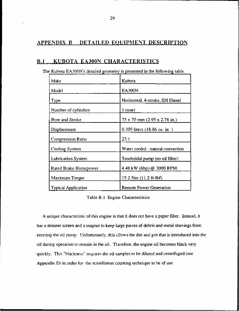
B.1 KUBOTA EA300N CHARACTERISTICS
The Kubota EA300N's detailed geometry is presented in the following table.
Make Kubota
Model EA300N
Type Horizontal, 4-stroke, IDI Diesel
Number of cylinders I (one)
Bore and Stroke 75 x 70 mm (2.95 x 2.76 in.)
Displacement 0.309 liters (18.86 cu. in. )
Compression Ratio 23:1
Cooling System Water cooled - natural convection
Lubrication System Trochoidal pump (no oil filter)
Rated Brake Horsepower 4.48 kW (6hp) @ 3000 RPM
Maximum Torque 15.2 Nm (11.2 ft-lbf)
Typical Application Remote Power Generation
Table B. I Engine Characteristics
A unique characteristic of this engine is that it does not have a paper filter. Instead, it
has a strainer screen and a magnet to keep large pieces of debris and metal shavings from
entering the oil pump. Unfortunately, this allows the dirt and grit that is introduced into the
oil during operation to remain in the oil. Th-erefore, the engine oil becomes black very
quickly. This "blackness" requires the oil samples to be diluted and centrifuged (see
Appendix D) in order for the scintillation counting technique to be of use.
30
B.2 RADIOACTIVE OIL [61
The tritiated oil received has been through a reduction process using tritium gas. This
gas, plus one ml of the neutral base oil, was mixed with forty mg of a platinum black
catalyst and stirred overnight. Afterwards, any labiles were removed using 50% benzene
methanol. The final result is the addition of tritium atoms to the hydrocarbon molecules in
the oil. This process is referred to as either a hydrogenation or tritiation process.
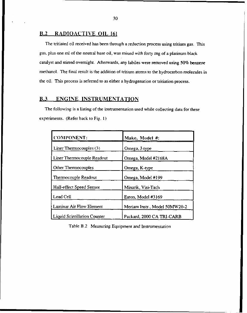
B.3 ENGINE INSTRUMENTATION
The following is a listing of the instrumentation used while collecting data for these
experiments. (Refer back to Fig. 1)
COMPONENT: Make, Model #:
Liner Thermocouples (3) Omega, J-type
Liner Thermocouple Readout Omega, Model #2168A
Other Thermocouples Omega, K-type
Thermocouple Readout Omega, Model #199
Hall-effect Speed Sensor Minarik, Visi-Tach
Load Cell Eaton, Model #3169
Laminar Air Flow Element Meriam Instr., Model 50MW20-2
Liquid Scintillation Counter Packard, 2000 CA TRI-CARB
Table B.2 Measuring Equipment and Instrumentation
31
APPENDIX C RADIOTRACER PROCEDURES
C.1 MIXING AND "BREAKING-IN" THE OIL
Non-radioactive oil should be mixed with radioactive oil until the concentration level is
approximately six microcuries per gram (6 gtCu/g). If a completely new batch of oil is
used, the engine should be operated for around 5 hours before any data samples are
collected. This break-in period allows any light ends to be burned off. (Refer back to
figure 9)
C.2 SAMPLING PROCESS
Before samples are taken, operate the engine continuously at the given load and speed to
allow temperatures to stabilize. Between speed changes, allow approximately 15 minute
for stabilization. After stabilization, run the vacuum pump for a short period of time in
order to draw exhaust gas through the sampling system. This is done (1) to ensure that the
engine and sampling system are making good water samples and (2) to ensure that any
water residue from the last data run is emptied from the condenser coils. The following is a
step-by-step description of the actual sampling process.
1) Replace water collection bottle with a clean one
2) Replace exhaust filter with a new one
3) Turn on the vacuum pump to initiate the sampling process
4) Measure and record the volume flow rate of fuel using the installed burette
and a timer
5) Record the pressure difference across the laminar flow element using the
installed inclined manometer
6) Record operating temperatures
7) After approximately ten minutes, secure from sampling by turning off the
vacuum pump. This time linit allows for:
32
a) collection of a sufficient amount of condensed water and
b) a sufficient number of piston ring revolutions and thus a better
average oil consumption
8) Remove both the filter and the water collecting bottle and replace with clean
ones (see Appendix D for preparation)
9) Stabilize at the next load and speed and repeat from step 3 on.
10) After running at the desired load and speeds, secure the engine and
drain approximately 50 ml of lubricating oil followed by draining one ml of oil
into a separate test tube (see Appendix D for preparation)
11) Return the 50 ml of drained oil to the sump
12) Record the barometric pressure and relative humidity
All data is recorded on available data shcets in the units indicated on the sheet. Using
these units allows the values to be inputted directly into the present spreadsheets (Appendix
E). Copies of the data sheets in use are included as the next two pages.
33
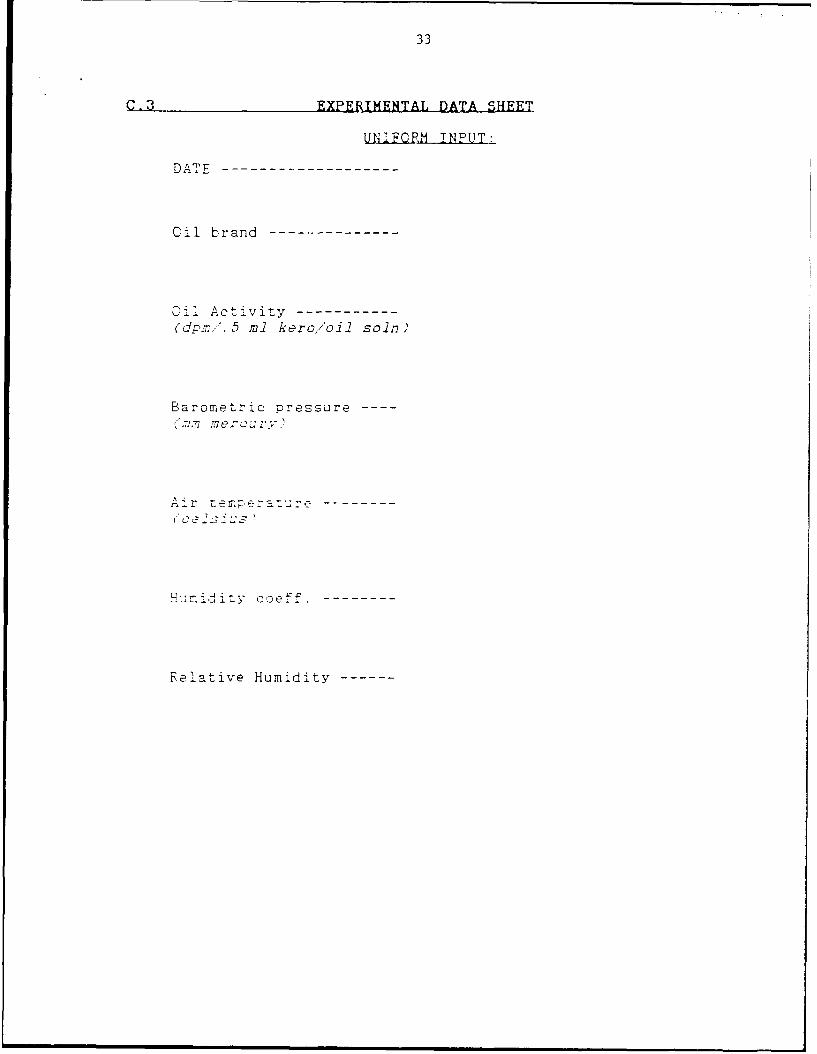
C.3 EXPERIMENTAL DATA SHEET
UNIFORM INPUT:
D^ADATE---------------------
Oil brand---------------
Oil Activity-------------(dpml. 5 ml kero/oil soln)
Barometric pressure
A£ 4
Air tempter ature--------
e v Humidity -----
Relative Humidity-------
34
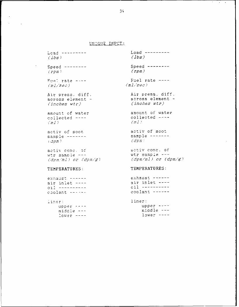
U _E INPUT:
Load - Load -
(ibs) (ibs)
Speed -------- Speed--------(rpm " (rpm)
_ rate ---- Fuel rate
(ml.io a 0) (mI.,.sec)
Air press. diff. Air press. diff.across element - across element -
(inches wtr) (inches wtr)amount of water amount of water
collected ---- collected(mld) (ml.)
activ of soot activ of sootsample sample-------( dpm ) (dpm
actjv conc. of activ conc. orwtr sample --- wtr sample
(dmm.- m .) or (dpr-,,' (dpm.'ml) or (dpm,'.)
TEMPERATURES: TEMPERATURES:
exhaust exhaust------air inlet air inletoil oil----------coolant coolant------
i er: liner:upper ---- upper
mi Ie --- middle
lower ---- lower
35
APPENDIX D SAMPLE PREPARATION [71
D.1 WATER SAMPLES
1) Filter the condensed water into a clean test tube
2) Add and mix a sufficient amount of ammonium hydroxide solution to the
sample to bring the PH up to 7 (neutral). [7,8]
3) Centrifuge the sample for approximately ten minutes
4) Filter again if necessary
5) Pipette 10 ml of fluor solution in'o a counting bottle
6) Pipette 1 ml of the water sample into the counting bottle (note - more or
less water may be counted but te spreadsheet is set up for 1 ml --see
Appendix E)
7) Replace top, mix, and number the sample
D.2 SOOT SAMPLES
1) Place the filter in a tube containing approximately 30 ml of fluor solution and
shake vigorously to mix well
2) Allow two hours for the fluor solution to dissolve the soluble hydrocarbons
and then shake again
3) Filter the solution into a clean te,:t tube. Repeat if necessary
4) Pipette 10 ml of the fluor solution into three counting bottles each
5) Divide the filtered solution among the bottles
6) Replace the tops, mix, and number the samples
D.3 OIL SAMPLES
1) Pipette 10 ml of kerosene into a clean test tube
2) Pipette .2 ml of the oil smnple into the kerosene. Subsequently. flush
36
the pipette with the oil/kerosene solution until all visible oil
residue is
removed from the pipette. Place pipette into the solution
3) Mix well and centrifuge for approximately ten minutes
4) Pipette 10 ml of the fluor solution into a counting bottle
5) Pipette .5 ml of the oil/kerosene solution into the counting bottle (note -
as before, more or less may be counted but the spreadsheet is set up for .5
ml -- see Appendix E)
6) Replace top, mix, and number the sample
All samples are taker to the Radiation Protection Office so that their activity levels may
be counted using a liquid scintillation counter.
37
APPENDIX E FORMULAS AND EXAMPLE CALCULATIONS
E.I OIL CONSUMPTION
E.la MEASURED CONSTANTS
pf = fuel density, g/ml = 0.838
Po = oil density, g/nl = 0.826 (15W-40) or 0.841 (SAE-30)
(1/C)f= hydrogen to carbon ratio of fuel = 1.8 (light diesel)
(H/C)0 = hydrogen to carbon ratio of oil = 1.88 (15W-40) or 1.78 (SAE-30)
LFE = Laminar flow element rating. CFM/in water
E.Ib CALCULATED CONSTANTS
Kr = water formation constant of fuel
= [g H20/g HI x [g H/ g fuel]
= [(2 + 16)/2] x f[(H/Crf/(12 + (II/C)f)]
= 1.174
Ko = water formation constant of oil
= 1.219 (15W-40) or 1.163 (SAE-30)
E.Ic MEASURED VARIABLES
Vf = volume flow rate of the fuel, ml/sec
dP = differential pressure across laminar air flow element, inches water
WA = amount of water condensed, ml
SAcw%' = specific activity of condensed water, dpm/ml
As = total activity of soot sample
SAo' = specific activity of oil/kerosene mixture, dpm/(.5 ml of oil/kero solution)
aim = barometric pressure, mm of mercury
38
Ta = air temperature, °C
11 = relative humidity, %
ELd CALCULATED VARIABLES
is = specific humidity, g H20/g air
= determined from psychrometric chart using H and Ta
Rf= wt rate of fuel. g/sec
= Vf x pf
It c = viscosity coefficient
= 1 - [.0025714 x (Ta - 20)] (note -- accurate for 15 < Ta < 35)
Pa = density of air, g/m 3
= (atm) x (133.32 Pa/mm Hg) x (28.962 g/mol) x (mol °K/8.3143 Nm) x
[1/(273 + Ta)OK] (note -- ideal gas law)
Ra = wt rate of air, g/sec
= (LFE) x (dP) x (.02832 m 3/ft3 ) x (min/60 sec) x [(aim)/29.92 in Hgj x
(in/25.4 mm) x (530 °R/[460 + (1.8Ta + 32)]°R} x et x Pa [8]
SAc 1 = total specific activity of exhaust sample, dpm/g
= SAc%%' + (As/V)
SAo = total oil consumption, g/hr
= [RfKf + Rahs]/[(SAcw/SAo) - Ko] x (3600 sec/hr)
E.2 OIL FLOW RATES (FROM FILM THICKNESS TRACES)
RPNI = revolutions per minute
V = average oil volume difference, for a given region, between the
power exchange strokes, nlm3/cycle
= calculated using an existing computer program which was modified
for the Kubota (Appendix F)
39
\'og average oil volume difference, for a given region, between the
gas exchange strokes, mm3/cycle
= calculated using an existing computer program which was modified
for the Kubota (Appendix F)
Vo = total avg. volume difference between the up and down strokes, mm3
= Vop + Nog
Rop) =rate of oil flow up the liner based on film thicknesses during the
power exchange strokes, g/br
(Vop) x (cm 3/1000 mm3 ) x (RPM) x (60 min/hr) x
(cycle/2 revolutions) x (po)
Rog rate of oil flow up the liner based on film thicknecses during tile
gas exchange strokes, g/hr
(Vog) x (cm 3/1000 lrun 3 ) x (RPM) x (60 min/hr) x
(cycle/2 revolutions) x (Po)
RO'= overall rate of oil flow up the liner based on film thicknesses, g/hr
= Rop +Rog
All of the preceding formulas are incorporated into LOTUS 123 v2.0 spreadsheets.
Examples of these spreadsheets are included as the following six pages. The first two
pages are for oil consumption calculations and the last four are for oil rates based on the
film thickness data.

4U
E.3 LOTUS 123 v2.01 SPREADSHEETS----------------------------
OIL CONSUMPTION CALCULATIONS:UNIFORM
INPUT CALCULATIONS
oil H/C ratio ---------- 1.78 / Oil formation constant --- 1.162554(SAE-30 = 1.78) /(15W-40 = 1.88) /
/
fuel H/C ratio --------- 1.8 / Fuel formation constant --l.i 7 3 9 13/
activ of oil smpl ----- 57052 / activ conc oil ----------- 6919505.(dpm/.5 ml soln) / (dpm/g)
/
oil density ------------ 0.841 /(SAE-30=.841) /(15W-40=.826) /
/
Barometric Pressure 777 /(mm mercury) /
/
humidity coeff --------- 0.01 /(lb wtr/lb air) /
/
air temperature 28 /(celsius) /
U IQUE
INPUT / CALCULATIONS/
Load (b) -------------- -7, / TOTAL oil consumption ---- 1.425019/ (g/hr)
Speed (rpm) ------------ 150 //
fuel rate ------------- -0.2C3 / fue rat_----------------0.170784(ml/sec) / (g/sec)/air pressure diff 1.275 / air rate ----------------- 3.29877(inches water) / (g/sec)
// equivalence ratio --------0.698150
"F/A)s = 0.0693
activ of s3ot smpl ---- 32 total activ of soot smp! - 632Idpm,'l mi -oin/ (dpm)
/
activ conc wtr smp---- 17i / total conc. of sample ----. :,..9(dpm/ml) or (dpm,'g) / (dpm/ml] or (dpm/g)
/
amount wzr :c1lected -- 2.9 /(ml) /
.ol w.nsump (burned) ----- . %31/ oil consump (nrurn) ------. 0267.
M Total ---------------------. 42490
42
OIL FLOWS UP THE LINER:
PISTON AVG VOL OIL FLOW AVG VOL OIL FLOW
REGIONS PWR STRK PWR STRK GS XCHNG GS XCHNG
SAE-30 (cu mm) (g/hr) (cu mm) (g/hr)
1500.00 I 1/2 crwn Ind (x2) 0.04 1.51 0.00 0.00
II top ring 0.01 0.38 -0.08 -3.03
III 1 ring width below 1.11 42.01 -0.23 -8.70
IV 2nd land 2.30 87.04 -0.52 -19.68V 2nd ring -0.02 -0.64 -0.11 -4.16
PISTON AVG VOL OIL FLOW AVG VOL OIL FLOWREGIONS PWR STRK PWR STRK GS XCHNG GS XCHNG
SAE-30 (cu mm) (g/hr) (Cu mm) (g/hr)
3000.00 I 1/2 crwn ind (x2) -0.34 -12.87 -0.12 -4.54II top ring 0.08 3.03 -0.21 -7.95IIi 1 ring width below 0.74 28.01 -0.23 -8.70IV 2nd land 1.43 54.12 -0.45 -17.03V 2nd ring 0.32 12.11 -0.19 -7.19
PISTON AVG VOL OIL FLOW AVG VOL OIL FLOWREGIONS PWR STRK PWR STRK GS XCHNG GS XCHNG
15W-40 (Cu mm) (g/hr) (cu mm) (g/hr)
1500.00 I 1/2 crwn ind (x2) -0.04 -1.51 0.08 3.03I: top ring 0.03 1.14 -0.04 -1.5111i 1 ring width below 0.63 23.84 0.05 1.89IV 2nd land 1.17 44.28 -0.08 -3.03V 2nd ring 0.16 6.06 -0.01 -0.38
PISTON AVG VOL OIL FLOW AVG VOL OIL FLOWREGIONS PWR STRK PWR STRK GS XCHNG GS XCHNG
15W-40 (cu mm) (g/hr) (cu mm) (g/hr)
3000.00 I 1/2 crwn lnd (x2) -0.22 -8.33 -0.16 -6.06II top ring 0.10 3.78 -0.20 -7.57III 1 ring width below 0.46 17.41 -0.38 -14.38IV 2nd land 0.91 34.44 -0.66 -24.98V 2nd ring 0.09 3.41 -0.35 -13.25
43
OIL FLOWS UP THE LINER:
PISTON AVG VOL OIL FLOWREGIONS ALL STRK ALL STRK
SAE-30 (cu mm) (g/hr)
1500.00 I 1/2 crwn ind (x2) 0.04 1.51II top ring -0.07 -2.65III 1 ring width below 0.88 33.30IV 2nd land 1.78 67.36V 2nd ring -0.13 -4.81
PISTON AVG VOL OIL FLOWREGIONS ALL STRK ALL STRK
SAE-30 (cu mm) (g/hr)
3000.00 i 1/2 crwn lnd (x2) -0.46 -17.41
II top ring -0.13 -4.92
III 1 ring width below 0.51 19.30
IV 2nd land 0.98 37.09
V 2nd ring 0.13 4.92
PISTON AVG VOL OIL FLOWREGIONS ALL STRK ALL STRK
15W-40 (cu mm) (g/hr)
1500.00 I 1/2 crwn ind (x2) 0.04 1.51II top ring -0.01 -0.38III 1 ring width below 0.68 25.73IV 2nd land 1.09 41.25V 2nd ring 0.15 5.68
PISTON AVG VOL OIL FLOWREGIONS ALL STRK ALL STRK
15W-40 (cu mm) (g/hr)
3000.00 I 1/2 crwn lnd (x2) -0.38 -14.38
II top ring -0.10 -3.78
III 1 ring width below 0.08 3.03
IV 2nd land 0.25 9.46
v 2nd ring -0.26 -9.84
44
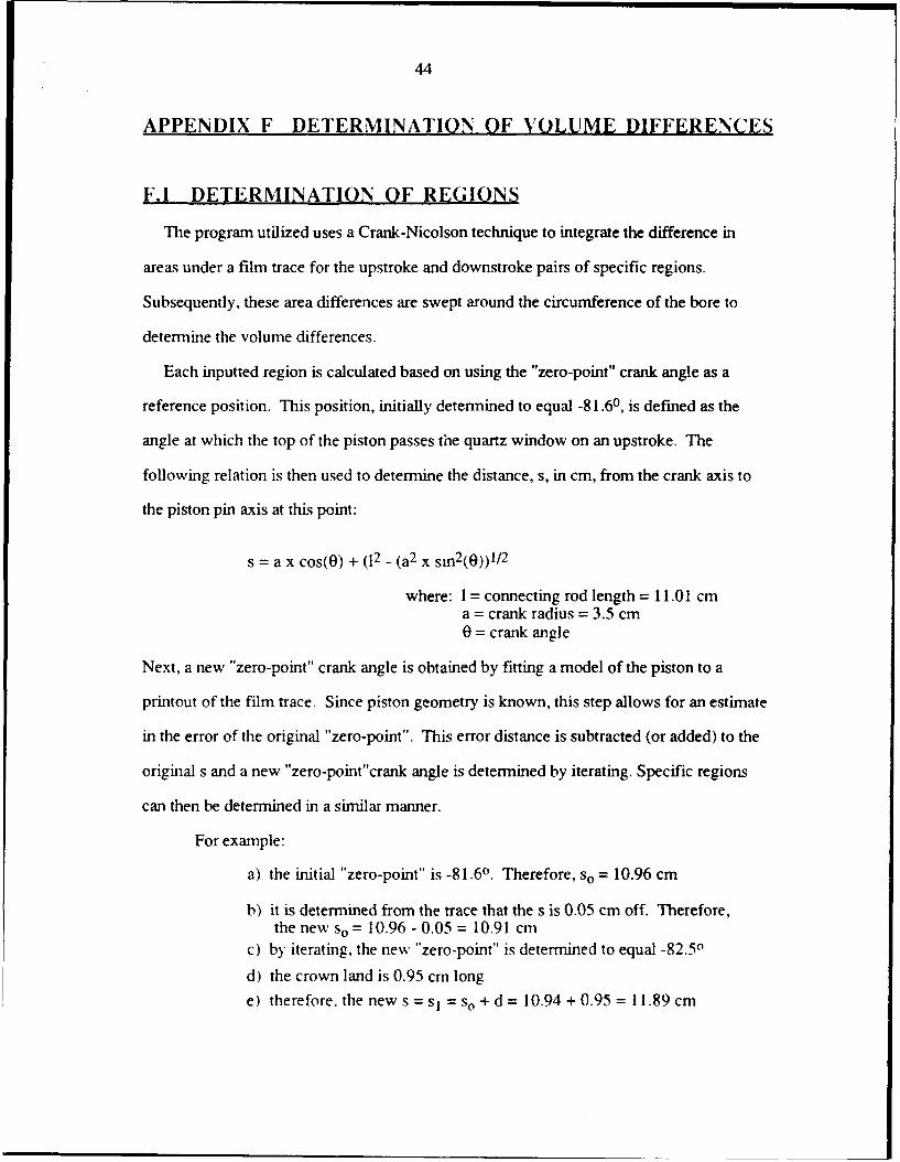
APPENDIX F DETERMINATION OF VOLUME DIFFERENCES
F.I DETERMINATION OF REGIONS
The program utilized uses a Crank-Nicolson technique to integrate the difference in
areas under a film trace for the upstroke and downstroke pairs of specific regions.
Subsequently, these area differences are swept around the circumference of the bore to
determine the volume differences.
Each inputted region is calculated based on using the "zero-point" crank angle as a
reference position. This position, initially determined to equal -81.60, is defined as the
angle at which the top of the piston passes the quartz window on an upstroke. The
following relation is then used to determine the distance, s, in cm, from the crank axis to
the piston pin axis at this point:
s = a x cos(0) + (12 - (a2 x si2(0)) 1/2
where: 1 = connecting rod length = 11.01 cma = crank radius = 3.5 cm0= crank angle
Next, a new "zero-point" crank angle is obtained by fitting a model of the piston to a
printout of the film trace. Since piston geometry is known, this step allows for an estimate
in the error of the original "zero-point". This error distance is subtracted (or added) to the
original s and a new "zero-point"crank angle is determined by iterating. Specific regions
can then be determined in a similar manner.
For example:
a) the initial "zero-point" is -81.60. Therefore, so = 10.96 cm
b) it is determined from the trace that the s is 0.05 cm off. Therefore,the new so = 10.96 - 0.05 = 10.91 cm
c) by iterating, the new "zero-point" is determined to equal -82.5o
d) the crown land is 0.95 cm long
e) therefore, the new s = s I = so + d = 10.94 + 0.95 = 11.89 cm
45
d) now iterate:0 = -67.70 implies s, = 11.850 = -67.90 implies st = 11.840 = -67.50 implies s, = 11.86 (correct one)
e) the region relating to the crown land would then be -82.50 to -67.50
f) the top ring region is determined in a similar manner except nowso = 11.91 cm
Regions IH, IV, and V consist of the top ring, second land, and second ring,
respectively. They are used to reflect the film behavior of the upper portions of the piston.
The crown land is not included based on the reasoning presented in section 6.2. Region I
is determined based on the film on the liner as three centimeters of the crown land pass the
window. The assumption is that the thickness on the liner at this point is the same up to
TRR (top ring reversal). Finally, region IIL, one ring width below the top ring, is used in
an attempt to substantiate the claim that oil is drawn up and around the top ring during
operation.
46
F.2 "MASSBAL.FOR" LISTING
CPROGRAM MASSBAL
CC ,,, Program to compute up / down stroke oil volume di'ferences inC distinct specified regions along the piston for multiple SloanC data files and write them to an output file that con beC converted to a bar graph format.CC This program requires as input any number of standard Sloan dataC files containing an array of position vs film thickness. The programC will average the volume of oil in any number of user specifiedC regions along the piston.cc The program has been adopted to analyze either McElweec (where IRDATE(3)-89] or Bliven flor.. data sets. Comandsc specific to Lux (where IROATE(3)-88] data sets have beenc neutralized by cocmment lines which are specified by "cc".c (M. Bliven. 14 March 199e]C
CC .,, Program structure:CC Main Level 1st Sublevel 2nd Sublevel 3rd SublevelCC MASSBAL FSTDGTPTC INTECRATCFC AVERZAGECC ,.. I/OCC Unit 3: INFILE Sloan data fileC Unit 5: Terminal IC Unit 6: Terminal 0C UNIT 10: OJTFILE. BDC LOCATIONS. RPMCC ,,. important variablesCC AVALS Array of average volume for like revolutionsC CALC Crank angle locationC NPAAX parameter. max number of points to plotC CALFCTR calibration factor for individual data setC CAOFFST correction factor for shaft encoder offsetC FILM(2.N 'PVkX) Array of position vs film thicknessC G - NVAL Mean value of oil volume difference for gasC exchange strokesC GESD Standard deviation for oil volume differenceC for gas exchange strokesC INFILEV Input file vectorC INTRFm Value for engine speed calculated from timeC difference between BDC pulsesC LWRB(10) Lower bound for region iC MNVAL Mean value of oil volume for a region for likeC revolutions from the program AVERAGEC NSDCLOC Batton dead center location in crank angleC NSTRCKE Number of strokes recorded in data fileC NUMFIL Number of Sloan files to processC NUR REG Number of regions to divide data intoC OFFST Instrument offset factor to initialize zeroC film thicknessC P"'NVAL Mean value of oil volume difference betweenC powered strokesC PWSD Standard deviation or oil volume differenceC between powered strokes
47
C REGVAL Array containing piston regions with theC average value of oil volume difference forC like revolutionsC SIGVAL Standard deviation of oil volume for likeC revolution from the program AVERAGE
CTE P(X-iee Imx Io onsc
PARAMJETER NPCMAX - 190000 1 max Iof points/cclPARAMETER NCMAX - 250~ I max# of cycles yclPARAMETER NRCMAX - 51mxofCce
CAAEE REMX-1INLDCLC*4FR otisI~II NEE.
CNLD SNO.C*IcntisIPII NEEsINCEs HD(5)IE226EIVLENe IHED ,NR.(IHED22NS6 TEQIAECCIE1NRNIE2NLTINEEs DAAN)4X
CNEE- DAANMXINEE 8CO(OA),NHIE SRK(CA)I NTEGERCH ISCLC(., CHI ,CALC(65 NTRKE(CM
$NRE.FPM(.NICMA.0AVI.ALO(.N4A).LE(2)S EA XOLD.XNW, NPMA(NO.4A). ,CAT.OLFF.APPT
S XSL(.E INTR(Ne~e)UTALoO).ROLUT.CAPTS XSL4 VL. FNTA.I.00VAL.OUloS. SIDVL. C, .ULLTS SLUTRVA. CRAD.MCROL, BO. CAOFFST. SICP(NREGWLO.$ LPSNREGMCKA. PW%.L(NBRE.GMAOF)T.WSNREO AXS CUPRB(NREGMAX). GESDA(NREGMAX), REGVA(NRE,.AX.NAX
C D4A(RGA) EDNEMXRGA(RGAXN)AX
CHARACTER INFILEV(2e).4e,CUTFILE.4e,A. ,B91.C.1,$ CALINT*3,STROE4,skip..3
CC ... iHal iza:
CALINT ' ON'ICH-
CC -* set up menu:C10 CONTINU.E
ISTAT - LISS$ERASE_..PAGE(1,1) I erase page ...WRITE (5,1000) CALINTREAD (S.e.ERR - 10.-"0 - 999) NCHOICE
CC see NCHOICE - 1: Set data files to readC
IF (NCHOICE.EQ.1) THENWRITE (6 ~ How many flor.e files? (up to 20):". )REA(5..) NUMFILDO I-I .NUMFILWRITE (6.'(" Enter filename 1 ''.12.*':*S)REA0(5. '(A4G0>) INFILEV(I)
END DOENDIF
CC see NCHOICE - 2: Set piston regions by crank angleC
IF (NCHOICE.EQ.2) THENWRITE (6,'(" How many piston regions? (up to 16): '))READ(5..) NlJMREGDO I-1,NLUREGWRITE (6,'(" Enter lower. then upper bound (CA deg) for
$ region j ".12.'': .. ).)1

48
READ(5,.) LWRB(I). UPRB(I)END DC
ENO I FCC see NCHOICE se 3: Linearly interpolate between crank anglesC
IF (NCHOICE.EQ.3) THENWRITE(6.'(1X-Linearly interpolate between crank angles?
$ (y/n)".$)')REAO(5, '(A1)') CIF (C.EO. Y* .OR.C.EO.'y') CALINT-'CNWIF (C.EQ. N .CR.C.EQ.'n') CALINT-0OFF'
END IF
C NCHCICE - 4: Check entered information see
CC Note: The running time of the program could be lengthyC depending on the number of data files and regions specified. It isC wise to cheek the input data for accuracy prior to execution.C
IF (NCHOICE.EQ.4) THENISTAT -LI8$ERASEPAGE(I.1) lerose pageDo 1 1, NUU4FIL
WRITE (6.'('' Data File 1 -.13." is: ".A4e)")I.$ INFILEV(I)
ENO0 000 1 - 1 . NL%OREGWRITE (6,'(" Crank angles bounding region )".12.
$ .. are: ",F7.2." to-.F7.2)')I. LWRS(I). UPRB(I)END DOWRITE (6. *(" RTN to continueREAD(5. G&1)') 9
END IFCC see NCHOICE - 5 Execute main program and write output.C
IF (NCHOICE.EQ.5) THENDO I - 1. NtMFIL
ISTAT - LIB$ERASEPAGE(1.1) lerase pageWRITE (5,1001) CALINT, INFILEV(I)ILLJN - 3OPEN(UNI T-I LUN. NAME-INFI LEV(I). TYPE-'OLD .ACCESS--DIRECT'
$ FORM-UNFORM4ATTED-)CC e'and read header:C
READ (ILUN-1) (IHE01(L).L-1,256)READ (ILUN-2) (IHED2(L).L-1,256)
CIDLU - 1MPPC - IDLA~sNBPC*256
CC see load up the private commnonCC These values are user specified prior to data collection.C
CAPPT se RUSER(26) I crank angles per pointLSTROKE -RUSER(27) I engine strokeSORE -RUSER(28) I engine bore I mCROL se RUSER(29) I connecting rod length m
CC see Convert to mm
49
CSCRE - BORE. 10.LSTROKE - LSTROKE*10.CROL - CRDL*IGCKRAD LSTROKE /2.
CC so* Set shaft encoder error in variable CAOFFST
C The shaft encoder marks the crank angle at BDC. Depending onC certain errors the recorded BDC position is not necessarily at -180.Cci IF (IRDATE(3).EQ.88) TH-Ncc CAOFFST - -178.5cc ELSE
if (irdate(3).eq.89.and.nrun.gt.99.and.nrun. lt.106) thenccoffst - -181
elseif (irdate(3).eq.90) thencooffst - -18e.926
elseCAOFFST - -180
endifendif
c ENDOIFCC ,.. Look for old 8ICIC file. The BDC file contains the specificC calibration factor and the number of revolutions in the dcta set.C
OUTFILE -ENCCCE(4.(''BDCLOC.''.I3)'.OUTFILE)NRUN
CC ... Open existing EDC fileC
OPEN(UNIT-1G.NIE-(JTFMLE, TYPE-'OL0".ACCESS-'SEOUENTIAL',S FOR FOMATTED ' )
READ(10,,) CALFCTR, NL5,WEVDO J -1 .NCMA.X
READ(10,.-ND-15, ER-5) NEDCLOC(J).INTRPF(J),NSTRCKE(J)ENDDO
15 CONTINUECC *, Set region along piston to analyzeC
DO N -1 . 2DO J-I.NLWEG
DO L-INUWEVREGVAL(JL) - 0.0
ENDDOENDDOM- 1DO K-N. NL REV-1, 2
IFPT-N6DCLOC(K)CC sea Set IFPT and NRPTS Set PCH for labelsC
NRPTS - NBDCLOC(K+I) - NBDCLOC(K) + 1 I # of points to readIF (NRPTS.GT.NPMAX) NRPTS - NPMAX
CC *,* Linearly interpolate between crank anglesC
IF (CALINT.EQ.'OFF') .OTO 21ICHI - I
C
50
CALL FSTDGTPT(ILUNICHI ,IFPT.NRPTSIDATA)C
NUP.4CA - eXOLD so CSCL(ICH1)*IDATA(1)+CBIA(ICHl)
c2 IF (NRUN.LT.47.and.irdate(3).eq.88) XOLD-XOLD-5.0cc IF (NkUN. 4 T.4.ana,.irdate(J).eq..'a) XCLD-AQLZ+5.0
skip so 'no,
DO L-2. NRPTSXNWs CSCL( ICHI ). DATA(L)-'iCSBIA( ICHI)
C3 IF (NR. ,i'LT.47.and.irda(3).eq.88) XNEW-XNEW-5.0cc IF (NRUN.GT.47.and.irda(3).eq.88) XNE*-XNEW+5.0
IF (XNE#.GT.2.5.ANO.X0LD.LT.2.5) THENif (cappt.eq..5.and.skip.eriyes') thenskip - 'no'go to 20
endifif (cappt.eq..5.ond.skip.eq.'no ') 3kip-'ye3'NLUJCA--NUM~CA+ 1CALOC(NIJUCA)-L + IFPT
20 ENDIFXC LD-XNEvY
ENCDO I ENO OF L LOOP FOR CRANK ANGLE LOCATION21 CONTINUZCC ... Average first iee data points of pmit signal toC establish zero offset. .005 sets this to 2 micronsCcl NOTE: This section adapted to analyze data collectedcc by SLIVEN whose PUT signal due to instrument offset andcc laser ref lectonces alone (ie. dry liner) was measured to becc approximately e.0e8 V. Averaging over first 100 data pointscc is by-passed and offset value is set to 0.008.cc
CALL FSTDGTPT(ILUN.ICH.IFPT.NRPTS.IDATA)c
if (irdate(3).aq.89) thenSLAd --a.DO L -300, 400VAL - CSCL(ICH.).IDATA(L) + CBIA(ICH)SUM so SUM + VALDI.MCT - L-299
ENCDO I END OF L LOOP FOR OFFSETC
OFFST - SLW4/DL'ICT-.016 I zero pt Offset for McElweeelseOFFST - .0 1 zero pt offset for Bliven
and i fCC *.Convert the data and write them into plot-arrayCC Note: CLKRTE is clock-rate in (kHz] and can be used toC convert x-oxi3 data timeC
DLPwLOT- CAOFFST0-1DO L so 1 ,NRPTS
CC .. Convert time to crank angle by speed or Position interpolationC
IF (CALINT.EQ.'OFF-) THENFILM(1.) - CACFFST + 360.sFLOAT(L-1)/FLOAT(NRPTS-1)
ELSE
C so* If Crank angle pj~lse is coincident with sample number, thenC increment x value by one crank angleC
IF ((L+IFPT).EQ.CALOC(Q)) THENFILM ''1 6; - CAOFFST + FLOAT(Q)DL7.4LT-F] LM(1. L)
ELSECC *'Otherwise divide fractions of crank angle evenly between pulsesC
IF (Q.EQ.1) THENF I IA( I.LQ - CAOFFST-,F LOA T(L-)/FLOAT (CA LOC(Q)- IFPT)
ELSEFILI4(1.L)-L.PLOT+LeO/FLOAT((CALOC(Q)-CALOC(O -l)))DLPLOT-F I W(I QL
END I FEND IF
ENDIFFIL.(2. L)-(CSCL(ICH).IOATA(L)+CSIA(ICH)-OFFST)/CALFCTR
cccccc write(S.'(-FIL)A(2.L) - -,fle.S)') film(2.l)ccc write(6, '(2i3.i6,2f82.)')n.k.l *fi lm(l1).film(2.l)ccc
LNOD CO I END OF L LOOP FOR FI ARRAY
C..Cal I ierct ion routine for each region. Program INTECRATDOFC: will calculate the volume of oil in 0 sPecifled region for oneC revolution.C
C-O J-1l. NLWEGCALL !NTEGPATE2DF(Fi LM.LWfRS(J) . UPRS(J) VALUE, NRPTSCiiCt.
$ CKRAO,)REGVAL(J.U) - VALUE(2).eORE.3.14159
c-cCC-_ write(62'(4i3.3el8.4)')m~n.k.j,vlue(l),value(2).regvol(j .m)ccc
EN CDO I END J LCOP FOR REGIONSAVALS(IJ.J) - VALUE(I1)
LENCO I END CF K LOOP FOR ALL REVOLUTIONS OF I TYPECC .. Call average routine for like revolutions af one region. ProgramC AVERAGE will calculate the overage volume for the like revolutions.C
DO J-1.NtiWEGDO L - 1 . NU.E EV
AVALS(2,L) - e.END CO
DO L-1,16AVALS(2,L) - REGVAL(J,L)
ENODOCALL AVERAGE(AVALS ,*JVAL,*JPOSSIGVAL, SIGPOS)IF (NSTROKE(N).EQ.l) THEN
PMA4NVAL(J) - I*4VALP WSD(J) - SIGVAL
ELSEGDJA4VAL(J) - lMNVALGESD(J) - SIGVAL
END IFENCDO I END OF J LOOP (DIFFERENT REGIONS)ENODO I END OF N LOOP (DIFFERENT REVOLUTION TYPES)
52
CC see Write output to a file with format massbal.# fileC
ENCODE (40.'(''[BLIVEN.DATA.MASS]MASSBAL.''.I3)',OUTFILE) NRUNOPEN (UNIT-le.FILE-OUTFILE.TYPE-'NEW',ACCESS-'SEOUENTIAL',F MC-.FORMArTEr)')
write (1,'(1x' . ')write (le.'(28x''I I '')*)write (10.'(28x''j , ASSBAL RESULTS )write (10.'(28x'-' "write (10.'(lx- -. )')write (1.'(28x''Dato Set: -',o15)')infilev(i)write (le,'(ix' . .')write (10.'(1x .. ..)')
WRITE(1,'(5X'' POWER STRCKES GAS$ ECHANGE-)')
write(10.'(5x"$ -I ))WRITE(1. '(5X''REG FRM TO MEAN STD DEV )JEAN
$ STO DE ')-)WRITE(10. (5X'' j (dog) (deg) (cu mm) (cu rmm) (cu mm)
$ (cu mr)' )')write(1e, (5x'
DO L -,1 NUNIREGwrite (Ie.'(1x" . ')WRITE (16.'(5X.I2,lX.F-7.2,2X.F7.2.4(3X.F7.2))')L. LWR8(L),
$ UPRB(L), PM&*AL(L). PWSD(L). GC,4VAL(L). GESD(L)LNCDCwrite (Ce. '(lx. 'write (10''(Ix'' .)')write (1 .'(lx. . '
write (Ie,'(ix'' . .'))write (10.'(tx''NCTE: If negative crank angle regions specified.
$ then POSITIVE mean values indi-ote '')')write (16,'(lx'' that UP3troke volumes are GREATER than
$ DCWNstroke volumes.'')')write (10,'(lx'" Standard deviations are always positive.'')*)ENODO I END OF I LO'P (MULTIPLE FILE)ENDIF I END OF NCHOICE 5 IF LOOP
CC ,,, Final BranchC5 CONTINUE
IF (NCHOICE.NE.e) GOTO 16C999 CONTINUECCC se Formats:C16e6 FORMAT (/" ,s OIL FILM STATISTICAL ANALYSIS ,,'///.
ST10,'(1) Enter files to analyze. ',/'STIe,'(2) Set piston regions. '*/,$T10,'(3) Linear Cronkangle Interpolation:',lxA3./,ST1.'(4) Check information for 1 & 2. ',/.$Tle,'(5) Compute averages and write to massbal file.'./,STle.'(6) or CTRLtZ for exit'///,$' Enter choice: '.$)
1661 FORMAT (/' see OIL FILM STATISTICAL ANALYSIS ,ee',///.$T10.'(1) Enter files to analyze. ',/.
53
STIe.'(2) Set piston regions. './,$TI.'(3) Linear Cronkongle Interpolation:',1x,A3./,$T1l.'(4) Check information for I & 2. './.$TlO,'(5) Processing file: ',A30.* Be Potientl',/,
or CTRLtZ for exit'///.S Enter choice: ',$)
STCPC
EDD
54
F. 3 'INTEC;-ATZ D-.1_0!,1' L TN
SIBFCTINE INTEGRATEOF (F"LM. LSD,UED.VALUE.NRPTS.CRDLCKRAD)CC *.This 3uboutine integrates the value in Fi lm(2. i) using the Crank-C Sicholsen nethod. It reads the step size from the first row ofC Film. The range is user-specified with lower and upper bounds.
C The difference between areas Of successive strokes is found and
C returned to the driver program for averaging.CC '.DIMF-ENSICN AND DECLARE VARIABLESC
PARAMETER NPMAX - 2!0000 1 max I of points/chPARAMETER NPCMAX - 60000 1 max #of points/cyclePARAMETER NCMIAX - 25e I maxi of cycles
CREAL F1 Li.(2.NPCWX) , LQ_,UED. VALUE(2) , ARE. PCSA, P058,
$CRDL. CKRAD. DWO~INTEGER 1,J,1<, NRPTS
CC *.SET INITIAL CCQNUIi IONS 8EFCRE INTEGRATINGC
J-16 K 1
DO I-1.NRPTS
K-I
cc:
cccELSE
rNC DOS CONT2NUE
CC ... Perform integration
AR EA - S.10 IF (FILM.(1.K+i).LE.U6D) THLN
POSA - CKRAD.CC S(FILM(I,K)/360..2..3.141593)+$SC-RTk'CR0L,*2 - (CKRAD..2).(SIN(FIL.(i .K)/360..2.3.141593))..2)
P052 - CKRAD.*CCS( FI LJJ( 1K+1)1360. e2,3. 14119)+SSCRT(CR0L..2 - (CXRAD..2).(SIN(FILMA(IK±1)/ZSS..2.3.14159))s.2)
C -' Divide by 1000. to convert microns to mmxrC
AREA-AREA+( (FT LM(2. K)+FI LM(2 K-.-l) )/1000.)$ A8S((P05B--PCSA)/2.)
K - <+1ccccc_- wri te(6. (3ei0.3) )posa.posb~area3c CZ
GCTO 10END IF
cccccc write(S, '(2fl0.3.ei0..3)')fi lm(l~k).fiim(2.k).areacc_^CC see Mirror bounds and find the area of the adjacent downstroke.C then subtract the values and return.C
IF (J.EO.i) THNOMEO - LBO
55
LED =-UEO
LiED - -ODVALUE(1) - AREAj -2GOTO 6
END I FVALUE(1) - VALUE(1) - AREAVALUE 2) - VALUE(l)
CC esReturn bound3 to original valuesC
DLBO - LEDLEID - -OiE
C *so That's the andC
RETURNEND
56
F.4 t1AVERAGE.FOR1' LISTLING
C SUBROUTINE AVERAGECAVALS.MVAL.MN~POS.SIGVAL.SIGPOS)
CC *so SUBROUTINE COMPUTES AVERAGE VALUES AND STANDARD DEVIATION
c PCR THE FEATURE OF INTEREST N PASSED IN MATRIX 'AVALS'
CC so* DIMENSION AND DECLARE VARIABLESC
PARMETER NPMAX - 250000 1 max i of points/ch
PARAMETER NPCMAX - 60000 1 max i of points/cycle
PARAMETER NCM.AX - 250 1 maxi of cycles
CREAL AVALS(2.NCIA~X).MNVAL,MNPOS,SIG\ AL.SIGPOS
$ XSUU. SUL4POS, XVAL. DUCT. XDEV. POSDEV , SOSUM. SOPSU
INTEGER I.J,KI-1
SU%(POS-60.le IF (AVALS(2,I).NE.O.0) THEN
XVAL - AVALS(2,I)XSt)4 - XSUM + XVAL
SUM4PCS - SUMPOS + AVALS(1.I)CMT- I
COTO 10END I FUNVAL - XSLU/CMCTMNPCS - SLW)CS/CMCT
C
12 IF(AVALS(Z.1).NE.e.0) THLN
XDEV - (AVALS(2.1) -4*iNAL)ee2
POSDEV -(AVALS(l1) - NC)-
S0Sum- SOSUiM + XDEVSDPSLU SCPSLW + PCSDEVCUCT - I1-1+1COTO 12
LND I FS I GVA L-SC-RT ( SDSUM./ZCT)S IGPCS-SlR T (SOPSUM/D44T)RETURN
CF-14D
57
INTAKE -.- Liner
Temperatures
Coolant Temperatures
0 Oil
TemperaturesLaminarFlow
E
Element __._ExhaustTemperature
gi - ENGINE
Temperature
To Sampling
Torque .System
RPM.
EXH ST
Figure 1. Engine Instrumnentation/Measurement Equipment
58
Top Ring:70 Half Keystone, I '-
EmbeddedChromium Strip
Scraper Ring:Tapered and Undercut ....
Oil Control Ring: Oil FlowOne Piece, Embedded HolChromium Strips on HoleRails, Slotted, with n-( aor andTension Spring behind
W r is t P in ...Centerline
Aluminum /Piston
Cast Iron [I5I .. .. Centerline
Figure 2. Piston and Rings of the Kubota EA300N
59
Measured MeasuredAirFlow 7 r1Fuel Flow
ENGINE(with radioactive oil)
I I Exhaust
'EXHAUSI , SampleEXHAU[ /- Line
TANKTo HouseExhaust ,
Filter Assembly
CondenserL (ice bath)
Vacuum WaterPump --- Collecting
Bottle
Figure 3. Schematic of Sampling System
60
S---- Add Radioactive _ _._
Oil
5 hours to burn off _, I i
Obtain samples inaccordance withAppendix C.
Prepare samples inaccordance withAppendix D.
F7n OilI
Motor enginewith flushing
oil
fl.ushing/
T yes
Motor engineDrain oil --- 0- with subsequent Drain oil
test oil
Figure 4. Procedural Flow Chart
61
OIL CONSUMPTION USING SAE-30(full load @ 1500 and 3000 rpm)
3.0j
2.61
: 2.2
C
C_ 1.8E
o 1.4
0
1.0
0.6- *
1000 1500 2000 2500 3000 3500RPM
Figure 5
62
OIL CONSUMPTION USING 15W-40(full load @ 1500 and 3000 rpm)
3.0-
2.6-
C,
.0
o. 1,4-
0
0.
1000 1500 2000 2500 3000 35 00RPM
Figure 6
63
GRAPH OVERLAY OF SAE-30 AND 15W-40OIL CONSUMPTION
3.0
2.6
., 2.2
Co 1.8. 8 ID 15W-40
E * SAE-30
- 1.4 -0
o 1 .0 - 0
0.6 ,
1000 1500 2000 2500 3000 3500
RPM
Figure 7
64
COMPARISON OF THE OIL CONSUMPTIONSUSING SAE-30 AND 15W-40
3
15 -4ElSAE-30
2 - .
E/
0
0-1500 2000 2500 3000
RPM
Figure 8
65
VOLATILITY OF NEW SAE-30(full load @1500 rpm)
3.0-
2.6-
EE
00
1.4-
0
1.0-
0.6ra12 3 4 56
TIME (hours)
Figure 9
66
STROKE COMP16 __ _ _ _ _ _ _ _ _ _ _ _
AVERAGE OF TEN COMP STROKES
.SAE-30, sto OC ring, 1500 RPM
0
C:9
LLJ
2
0
-5 0 5 10 15 20
DISTANCE ALONG PISTON (mm)
Figure 10
67
STROKE:EXP
AVERAGE OF TEN EXP STROKES I14 SAE-30, std CC rtng, 1500 -,
12
0 -
2:
-20 - 15 -10 -5 0
DISTANCE ALONG PISON (mmn
Figure 11
68
STROKE:EXH
AVERAGE OF TEN EXH STROKES
14 SAE-30, std OC ring, 1500 RPM
12
C-
10 5 10 27 PT
.ISTANCE ALONG PISTON ( m m
Figure 12
69
STROKE: •NT
AVERAGE OF TEN INT STROKES
14 SAE-30 std OC ring, 1500 r~m
E(-)
10V0
/TT.N' ALNO PI4 O (rim)
/u 1
4f- -i/I-
DISTANCEr Ar , PISON (rmW
Figure 13
70
Liner
A
Liner
Liner 11 1
Figure 14. Areas/Volumes of possible oil
consumption mechanisms
71
LABELED REGIONS OF COMP STROKE:
: SAVERAGE CF TEN COMP STROKES
I SAE-30, std OC rtng, 1500 RPM
12
zi 4
~REGION I: (representative of the liner as the
2 crown land passes)
44
0 1 2 3 4 5 7 8
DISTANCE ALONG PISTON (mm)
Figure 15
72
LABELED REGIONS OF COMP STROKE:
16 OF* TEN I IiiAVERAGE OF TEN COMP STROKES
14 SAE-30, std OC rPng, 1500 RPM
12
10
REGION IV:
REGION II: REGION III-
6REGION V:
4 -"H 7
2
8 10 11 L1 13 14 15 16 17 1
DISTANCE ALONG PISTON (mm)
Figure 16
73
OIL FLOW FOR THE POWER EXCHANGE STROKESUSING SAE-30 AT 1500 AND 3000 RPM
100-
80" 1500 RPM SAE-30
0 3000 RPM SAE-30uJ 60z
i- 40
0 20
U-
-20oil cons. 1 II III IV V
PISTON REGION
Figure 17
74
OIL FLOW FOR THE POWER EXCHANGE STROKESUSING 15W-40 AT 1500 AND 3000 RPM
100
=1500 RPM 15W-40
wU 60 El3000 RPM 15W-40
w
0-
0 20
0 0
-j-
oil cons. 1 11 111 IV VPISTON REGION
Figure 18
75
OIL FLOW FOR THE GAS EXCHANGE STROKESUSING SAE-30 AT 1500 AND 3000 RPM
-20-
0U -40
-2
-
DU 1500 RPM SAE-30-60 - 3000 RPM SAE-30
0LL
S-80-0
oil cons. I IIIIV VPISTON REGION
Figure 19
76
OIL FLOW FROM THE GAS EXCHANGE STROKESUSING 15W-40 AT 1500 AND 3000 RPM
20-
- 0-
w -20-Z
I--40-
o -60 U 1500 RFM 15W-40U. 3000 RPM 1 5W-40
0 -80-
-1001oil cons. I II 111 IV V
PISTON REGION
Figure 20
77
OIL FLOW FOR ALL STROKESUSING SAE-30 AT 1500 AND 3000 RPM
100
80-
U1500 RPM SAE-30
U60 C 3000 RPM SAE-30z
~40-
0 20-
0 0
-20-oil cons. I IIII IV V
PISTON REGION
Figure 21
78
OIL FLOW FOR ALL STROKESUSING 15W-4C AT 1500 AND 3000 RPM
100-
80-
U1500 RPM 15W-40
S60 5 3000 RPM 15W-40wz
wLZ40-
0 20-j
-2
oil cons. I IIII IV VPISTON REGION
Figure 22
79
NON-DIMENSIONALIZED OIL CONSUMPTIONAND REGION 11 VALUES FOR POWEREXCHANGE STROKES USING SAE-30
0X,
-6 non-dim 1500 RPM SAE-30
13 non-dim 3000 RPM SAE-30
0
0.
0 ' o / ./ /
0~ 2igure 2/
80
NON-DIMENSIONALIZED OIL CONSUMPTIONAND REGION II VALUES FOR POWER
EXCHANGE STROKES USING 15W-40
LO
6 c non-dim 1500 RPM 15W-40
4) non-dim 3000 RPM 15W-40
>4
a-
Ci
0 2 "
0
cc
oil cons. PISTON REGION
Figure 24
81
OIL FLOW RATES OF THE UPPERHALF OF THE PISTON
200
m U SAE-30
10 15W-40
w
w
0
-JLL
100
PWR-1500 PWR-3000 GAS-1500 GAS-3000STROKE PAIRS - RPM
Figure 25
82
RPM vs. UPPER LINER TEMPERATURES180
170
cc:3
._
ujWJ 160
I-
uJ 150I-
1401000 20C0 3000 4000
RPM
Figure 26
83
VISCOSITIES OF SAE-30 AND 15W-40vs. RPM
7 -0 SAE-30 High Shear visc- 1 5W-40 High Shear visc
U- SAE-30 Low Shear visc-0-- 1 5W-40 Low Shear visc
5 -
WlW 4
3:-
21000 2000 RPM 3000 4000
Figure 27
84
SURFACE TENSION vs.RPM
0.01 7J
z0.016-
0
0 .05
0.0141000 20G0 3000 4000
RPM
Figure 28
85
VISCOSITIES vs. OIL CONSUMPTIONS
7.
6 - HS SAE-30
- - HS 15W-40
--- LS SAE-30
'fl •5LS 1SW-40
. 0
04-
o
2 *
0 1 2 3
oil consumption (g/hr)
Figure 29