ibero-amerika institut für wirtschaftsforschung instituto ... · vary between one and ten years,...
TRANSCRIPT

Ibero-Amerika Institut für Wirtschaftsforschung Instituto Ibero-Americano de Investigaciones Económicas
Ibero-America Institute for Economic Research (IAI)
Georg-August-Universität Göttingen
(founded in 1737)
Nr. 125
The Free Trade Agreement between Chile and the EU: Its Potential Impact on Chile’s Export Industry
Felicitas Nowak-Lehmann D., Dierk Herzer,
Sebastian Vollmer
November 2005
Diskussionsbeiträge · Documentos de Trabajo · Discussion Papers
Platz der Göttinger Sieben 3 ⋅ 37073 Goettingen ⋅ Germany ⋅ Phone: +49-(0)551-398172 ⋅ Fax: +49-(0)551-398173
e-mail: [email protected] ⋅ http://www.iai.wiwi.uni-goettingen.de


The Free Trade Agreement between Chile and the EU:
Its Potential Impact on Chile’s Export Industry
By
Felicitas Nowak-Lehmann D.: Ibero-America Institute for Economic Research, [email protected], Dierk Herzer: Ibero-America Institute for Economic Research, [email protected] and Sebastian Vollmer: Ibero-America Institute for Economic Research, [email protected]

2
Abstract Bilateral Free Trade Agreements (FTAs) and unilateral trade liberalization have been two
strategies used extensively by Chile to expand its exports and improve its competitive position
in the world markets. It is the objective of this paper to analyze the role of trade agreements,
price competitiveness, real income, per capita income differences and transport costs in
Chilean export trade with the EU. To this end, Chile’s most important export sectors, namely
fish, fruit, beverages, ores, copper, and wood and products thereof are investigated using
panel data from Chile’s main trading partners in the EU over the period 1988-2002. The
econometric model used is a refined augmented gravity model. It is found that the FTA
between Chile and the EU, if fish, fruit and wine were included, would have a noticeable
impact on Chilean export performance. Price competitiveness is important in most of the
sectors under investigation. As expected, the relevance and impact of transport costs on
exports do vary from sector to sector.
Keywords:
EU-Chile trade agreement, sectoral trade flows, gravity model, panel analysis
JEL: F14, F17, C23

3
The Free Trade Agreement between Chile and the EU:
Its Potential Impact on Chile’s Export Industry
1. Introduction
Chile initiated unilateral trade liberalization in 1975 and is now one of the most open
economies in the world. Between 1975 and 1979, exports and imports represented just 38.6%
of GDP, whereas in 1996-2004 the foreign trade ratio rose to 62.5%. Chile also followed a
rigorous strategy of signing bilateral trade agreements. Since 1990, Chile has concluded many
trade agreements with other Latin American countries. It is an associate member of
MERCOSUR (Argentina, Brazil, Paraguay and Uruguay) and has signed bilateral trade
agreements with Bolivia, Colombia, Cuba, Ecuador, Mexico, Peru and Venezuela as well as a
trade agreement with the Central American countries. Free Trade Agreements (FTAs) with
developed countries such as the United States, the European Union (EU), Canada, South
Korea and EFTA have been signed since 2000. In May 2005 Chile started negotiations on a
Free Trade Agreement (FTA) with China, a P4 Strategic Economic Partnership Agreement
with New Zealand, Singapore, and Brunei Darussalam, and a Partial Scope Trade Agreement
with India. Furthermore, a feasibility study for an FTA with Japan has already been made. In
practical terms, these treaties have expanded the size of Chile’s market from 15 million
inhabitants to around 1.3 billion worldwide (Chile Foreign Investment Committee, 2005).
In order to enhance economic cooperation with the EU and expand into European markets,
Chile signed a far-reaching FTA with the EU on 3 October 2002. Following the approval of
the Association Agreement by the EU Council and Chile on 18 November 2002, and after
ratification by the Chilean Congress, the trade chapter of the Association and Free Trade
Agreement came into force on 1 February 2003 (European Parliament, 2005). The agreement
implies the total liberalization of tariffs and non-tariff barriers affecting trade in goods
(excluding only some fishing and agricultural products) but contains transitional phases that
vary between one and ten years, depending on the product. After the fourth year of
implementation, the agreement will eliminate tariffs on 96% of Chile’s exports to the EU and,
based on EU-25 figures, improve Chile’s access to a market of more than 456.8 million1
consumers (Chile Foreign Investment Committee, 2005).
1 Inhabitants on 1 January 2004.

4
The FTA between Chile and the EU, once fully implemented, will be beneficial to both the
EU and Chile.2 With respect to trade, the EU expects a major expansion of its manufactured
exports to the Chilean market, whereas Chile hopes to expand its agricultural and light
manufactured exports to the EU.
From Chile’s point of view, the agreement can be clearly considered as a means to maintain
and/or strengthen its competitive position in the EU market. In the short run, a reduction or
elimination of trade barriers through an FTA and its impact on relative prices will improve
Chile’s competitive position not only with respect to the EU countries but also with respect to
third countries that do not have an FTA with the EU. In the medium to long run however, the
effect of the FTA will be eroded if the EU also decides to conclude FTAs with countries like
Brazil, Argentina, Paraguay, Uruguay, Bolivia, Peru, and perhaps some Asian countries. In
addition, Chile has numerous competitors worldwide3: Norway, Russia, Indonesia, Malaysia,
the Philippines and Thailand are, much like Chile, exporters of timber and rubber. The
Southeast Asian countries have been able to significantly increase their light manufactured
exports to industrial countries in the last decade. In the Southern Hemisphere, South Africa,
Australia and New Zealand threaten Chile’s position as a successful fruit and wine exporter.
In agricultural products, Chile faces stiff competition from the EU countries. UK, Ireland and
Norway are Chile’s main competitors as far as fish exports are concerned. Furthermore, with
its low labor costs, China has become a strong exporter of machinery and equipment, textiles
and clothing, footwear, toys and sporting goods and mineral fuels, thus reversing Latin
America’s competitiveness in textile, clothing and shoe exports.
Based on 2003 data, the EU is Chile’s top trading partner worldwide. 25% of Chile’s exports
go to the EU and 19% of its imports come from the EU. During the first semester of 2003,
mining (predominantly copper) still represented 46% of total Chilean goods exports, while
agriculture, farming, forestry and fishing products represented 13.02% thereof. Trade with
Chile represents 0.45 of total EU trade, putting Chile in 41st place among the EU’s top trading
partners. Between 1980 and 2002, EU imports from Chile increased from €1.5 billion to €4.8
billion, while EU exports to Chile increased from €0.7 billion to €3.1 billion.
Chile’s main export commodities comprise copper, fish, fruits, paper, paper pulp, and wine
and are thus heavily natural resource based. Its main import commodities include consumer
goods, chemicals, motor vehicles, fuels, electrical machinery, heavy industrial machinery and
2 Next to trade facilitation through reduction and elimination of tariffs and modern customs techniques, it comprises economic co-operation and technological innovation, protection of the environment and natural resources and support for government reforms (http: europa.eu.int/comm./external_relations/chile/intro/ index.htm; 16 February 2005). 3 Chile is still considered the most competitive and the least corrupt economy in Latin America.
5
food. Chile applies low import tariffs (6% in 2003) and non-tariff barriers are not important
due to the establishment of a liberal and transparent trade regime in 1974. The unilateral trade
liberalization that Chile went through from 1975 to 20044 implied the quasi-abolition of non-
tariff trade barriers and the imposition of uniform tariffs.
Only very few studies exist on the impact of the FTA between Chile and the EU. The study of
Chumacero, Fuentes and Schmidt-Hebbel (2004) examines the FTA’s impact on growth,
factor productivity, aggregate investment, country risk premium and the government budget,
by means of a three-sector model dynamic general equilibrium model. The authors find that
the effects of the EU-Chile FTA on resource allocations, relative prices, expenditure
composition, welfare, output, and aggregate consumption do not exceed 1% in any given
period. Aggregate imports and exports grow by 2.7% and 20% respectively, and the real
exchange rate depreciates by 0.2%. A lower risk premium leads to a temporary consumption
and investment boom that is reversed in the long run as a result of larger net foreign liabilities.
Another major finding is that, in the steady state, the gains from improved factor productivity
outweigh all other effects. SIA Chile-EU (2002) estimates the welfare effect of the FTA
between Chile and the EU to be 0.5%. Harrison et al. (2003) estimate the combined free trade
effect with NAFTA, MERCOSUR, the EU, and the rest of South America to range between
2.66% and 5.71% as a fraction of GDP. The above-mentioned studies all develop and use
multi-sector computable general-equilibrium (CGE) models for Chile, but do not sufficiently
consider the FTA’s impact on the production structure or on sectoral exports. We try to fill the
gap by looking closely at the FTA’s impact on Chile’s most important export sectors. Partial
equilibrium models will be used instead of CGEs.
The objective of this paper is to analyze Chile’s most important export sectors and to evaluate
its export strength on the EU market in the period 1988 to 2002. The empirical model used is
an extended version of the gravity model that takes price competition5, trade barriers and trade
preferences, real incomes, real per capita income differences, and transport costs in the export
trade between Chile and the EU into account. Starting from an assessment of underlying trade
structures and the determinants of current trade flows between Chile and the EU, an export
trade analysis will be performed for the Chilean economy. Finally, the impact of the Chile-EU
trade agreement on Chile’s exports will be simulated and discussed.
4 Trade liberalization was interrupted during the debt crisis and the economic recession of the period 1982-1985. 5 Price competition in the EU market will be examined by looking at price competition from both the EU countries and the South East Asian + Southern Hemisphere countries as well as Norway.

6
The study is structured as follows. Section 2 gives an overview of Chilean exports under
analysis, its structure and dynamism and Chilean competitors in the EU market. In Section 3,
we present our extended version of the gravity model with its focus on export flows in real
terms. Section 4 contains the empirical application of the gravity model to Chile-EU trade and
the estimation and simulation results. Section 5 concludes.
2. Chile’s exports to the EU and its market share in the EU market
In Table 1 we list Chile’s largest export sectors.
Table 1: Chile’s seven most important export products
HS
code
Sector Av.
export
value
in mill.
current
ECU
(1988-
2002)
Export
value in
mill.
current
ECU in
2002
Annual
percentage
change of
exports
(1988-
2002)
Export
share
in
20026
Potential
extra-EU
competitor
Average
market
share in
the EU7
(1988-
2002)
03 Fish and
crustaceans,
molluscs
142.6 247.0 7.2 % 5.2 % Norway 1.22 %
08 Edible fruit
and nuts
371.5 476.6 7.5 % 10.0 % South
Africa,
Australia,
New
Zealand
2.62 %
22 Beverages,
spirits and
vinegar
125.4 373.4 44.6 % 7.8 % South
Africa,
Australia
0.77 %
26 Ores, slag
and ash
331.3 434.9 11.9 % 9.1 % Australia,
Brazil,
China
3.75 %
6 Share of Chile’s sectoral exports in total Chilean exports. 7 Share of EU imports from Chile in total EU imports (both from other EU-countries and non-EU countries).

7
44 Wood and
articles of
wood
51.5 70.7 12.4 % 1.5 % Norway,
Russia,
Canada,
Malaysia,
Indonesia
0.26 %
47 Pulp of
wood
224.3 315.6 13.9 % 6.6 % Norway,
Canada,
Russia
2.89 %
74 Copper and
articles
thereof
1,285.6 1,767.9 5.4 % 37.0 % South
Africa,
Canada
10.34%
Source: EUROSTAT (2003); COMEXT CD ROM, ‘Intra- and Extra-EU Trade, Annual data, Combined
Nomenclature’, European Commission ; own calculations.
We consider averages of sectoral export values over the period 1988 to 2002 in order to
smooth out peaks and valleys. As far as agriculture is concerned, we selected sectors with an
export value of more than 200 million ECU (yearly average 1988-2002). Pre-selection of the
seven sectors was based on Chile’s 30 largest sectors in 2002.
All seven of the sectors with a considerable export value also experienced remarkable export
growth, beverages being the most dynamic sector with an annual growth rate of around
44.6%. It should be noted, however, that ‘beverages’ started from a lower level in 1988 than
the more traditional sectors such as fruit, wood, pulp of wood, and copper.
Copper has the biggest market share of EU imports with 10.34%, followed by ores (3.75%),
wood pulp (2.89%) and fruit (2.62%) in the period 1988 to 2002.
The development of sectoral exports will be discussed and analyzed in Section 4, where
summary tables will also be presented.

8
3. The augmented gravity model for modeling export flows
3.1 Data and model set-up
In the econometric part of this study, we use EUROSTAT’s trade database COMEXT (Intra-
and Extra-EU Trade, Supplement 2, 2003). The analysis has to be restricted to six EU
countries: France, Germany, Italy, the Netherlands, Portugal, Spain and the UK. Due to
incompleteness of the data, we excluded nine EU-15 countries and all ten EU-108 countries
from the analysis. Wood, wood articles, and wood pulp must be exempted from the
econometric analysis9 due to illegal logging that caused prices to lose their signaling function.
We subject five export sectors—fish, fruit, beverages, ores and copper (at the two-digit level
of the Harmonised System (HS) classification)—to econometric analysis. The period covered
is 1988 to 2002. We have a maximum of six cross-sectional10 trade flows and 15 years,
resulting in a maximum of 90 observations per sector. The number of observations varies
depending on the product studied. Sources and compilation of the data are outlined in the
Appendix.
Following Martínez-Zarzoso, I. and F. Nowak-Lehmann D. (2003, 2004), we utilize a variant
of the gravity equation to model bilateral export flows from Chile to the EU and have added
some refinements. A log-log specification of the gravity model is selected for Chilean exports.
According to the generalised gravity model of trade, the volume of exports between pairs of
countries, Xij, is a function of their incomes (GDPs), their populations, their geographical
distance and a set of dummies,
ijijijjijiij uADNNYYX 6543210
βββββββ= (1)
where Yi (Yj) indicates GDPs of the exporter (importer), Ni (Nj) are populations of the
exporter (importer), Dij measures the distance between the two countries’ capitals (or
economic centres) and Aij represents any other factors aiding or preventing trade between
pairs of countries. The error term is uij. An alternative formulation of equation (1) uses per
capita income instead of population,
8 The EU-10 countries have not yet been integrated into the COMEXT trade statistics thus impeding their analysis. 9 We did, however, carry out a descriptive analysis of Chile’s market shares. 10 But not in all sectors! For example, there is a large amount of missing data on Portugal’s imports in sectors 07 and 20.

9
ijijijjijiij uADYHYHYYX 6543210
γγγγγγγ= (2)
where YHi (YHj) is exporter (importer) per capita GDP.
We deviate from the generalised gravity model in several respects. First, we do not focus on
infrastructure and in particular not on terrestrial infrastructure (i.e., the circumstances of
arriving at the domestic port and departing from the foreign port), but on maritime transport
costs when measuring distance. For this purpose, we scaled geographical distance (actual
nautical miles) using the freight cost index to construct a new transport cost variable. We
assumed that merchants would use sea transport whenever possible, given the fact that a
certain quantity transported by ship (40-foot containers) costs about one-fifth of the same
quantity transported by road (13.6-meter trailer). We do not consider land transport costs here
since they are the same for all exporting countries and independent of the export port (Chile,
Norway, Indonesia) once the destination (foreign) port (e.g., Hamburg) has been reached. But
still it has to be noted that land transport costs of the exporting country (e.g., Chile, from
Talca to Concepción) will differ from exporting country to exporting country (Chile, Norway,
Indonesia) and should therefore be considered. However, they are partly incorporated into the
income variable of the exporting country. A country with higher GDP will also have better
public infrastructure.
In this study, we also examine whether transport costs influence exports in a linear or non-
linear way. As to the latter, increasing knowledge about how to organize transport could cause
each additional unit of transport costs to have a progressively decreasing effect on exports.
Moreover, higher transport costs might enforce the more efficient use of port facilities,
containers and personnel, and might therefore lead to an underproportional negative impact on
exports. We also believe that sectoral differences can be found in the relationship between
transportation costs and exports, depending on the products under investigation and the
weight of transport costs in the value of exports. It might, for example, be more difficult to
organize the export of frozen or smoked fish than of ores and copper. The export of fish
requires modern containers with a refined cooling system, punctual forwarding agents,
reliable carriers and shipping agents, and better knowledge of the importing country’s port
and road infrastructure and people’s tastes than the export of minerals. The IDB Report
(2001) points to the importance of transport costs for Latin American trade. It claims that the
effective rate of protection provided by transport costs is often higher than the rate provided
by import tariffs. As for Chile, import tariffs represent less than 1% of the value of its exports
to the United States, while transport costs are 12% or more of that value. Anderson and

10
Wincoop (2004) emphasize the importance of trade costs for trade flows. They compute
transportation costs (a component of trade costs) to amount to a tariff equivalent of 21%,
based on estimates for U.S. data. However, they also mention the high variability of trade
costs across both goods and countries.
Second, concerning economic distance, we use differences in incomes between trading
countries, a variable similar to that used in Arnon et al. (1996) and in McPherson et al. (2000).
Our variable is constructed as the absolute difference in per capita incomes in purchasing
power parities (PPP).
We can identify two conflicting effects of this variable on trade. On the one hand, on the basis
of the Linder (1961) model, when the trading countries have very different per capita
incomes, lower economic distance might foster trade. With this effect, the more similar their
per capita incomes, the more countries tend to increase their bilateral trade in similar
products. We therefore expect more trade to be intra-industry trade (countries should both
export and import the same goods) when per capita incomes converge.
On the other hand, if we consider the Heckscher-Ohlin (H-O) model, higher economic
distance might foster inter-industry trade (countries import and export different goods). H-O
focuses on expected trade patterns when countries have different factor endowments but
similar tastes. Per capita income differences can represent inter-country differences in factor
scarcity.
We assume that current trading patterns are affected by both factors. For some commodities,
we expect that the Linder effect dominates the H-O effect and that economic distance has a
negative effect on trade. For other commodities, the opposite might occur, in which case
economic distance would have a positive effect on trade.
Finally, we add a real exchange rate variable to our specification (Bergstrand, 1985, 1989;
Soloaga and Winters, 1999). We calculated Chile’s and its competitors’ bilateral real
effective11 exchange rates (price quotation system) taking into account protection. Average
tariffs imposed by the EU and EU subsidies enter the formula (see WTO Trade Policy Review
European Union, Vol. 1, 2000, page 101). All the calculations are shown in the Appendix.
Exports from country i to country j in period t of commodity k are then modelled as a log-log
function:
11 Effective implies that EU import tariffs and subsidies are taken into account. This definition differs from the IMF definition, which understands real effective exchange rates as multilateral trade-weighted real exchange rates.
11
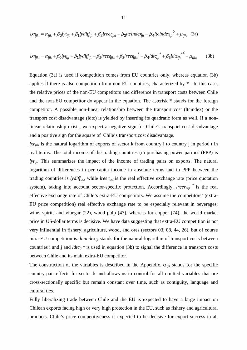
ijktijtijtijktijtijtijkijkt ltcindexltcindexlreerlydifflytlxr µβββββα ++++++= 243210 (3a)
ijktijtijt*
ijktijktijtijtijkijkt ldtcldtclreerlreerlydifflytlxr µββββββα +++++++=2
543210** (3b)
Equation (3a) is used if competition comes from EU countries only, whereas equation (3b)
applies if there is also competition from non-EU-countries, characterized by * . In this case,
the relative prices of the non-EU competitors and difference in transport costs between Chile
and the non-EU competitor do appear in the equation. The asterisk * stands for the foreign
competitor. A possible non-linear relationship between the transport cost (ltcindex) or the
transport cost disadvantage (ldtc) is yielded by inserting its quadratic form as well. If a non-
linear relationship exists, we expect a negative sign for Chile’s transport cost disadvantage
and a positive sign for the square of Chile’s transport cost disadvantage.
lxrijkt is the natural logarithm of exports of sector k from country i to country j in period t in
real terms. The total income of the trading countries (in purchasing power parities (PPP) is
lytijt. This summarizes the impact of the income of trading pairs on exports. The natural
logarithm of differences in per capita income in absolute terms and in PPP between the
trading countries is lydiffijt,, while lreerijkt is the real effective exchange rate (price quotation
system), taking into account sector-specific protection. Accordingly, lreerikjt * is the real
effective exchange rate of Chile’s extra-EU competitors. We assume the competitors’ (extra-
EU price competition) real effective exchange rate to be especially relevant in beverages:
wine, spirits and vinegar (22), wood pulp (47), whereas for copper (74), the world market
price in US-dollar terms is decisive. We have data suggesting that extra-EU competition is not
very influential in fishery, agriculture, wood, and ores (sectors 03, 08, 44, 26), but of course
intra-EU competition is. ltcindexijt stands for the natural logarithm of transport costs between
countries i and j and ldtcijt* is used in equation (3b) to signal the difference in transport costs
between Chile and its main extra-EU competitor.
The construction of the variables is described in the Appendix. αijk stands for the specific
country-pair effects for sector k and allows us to control for all omitted variables that are
cross-sectionally specific but remain constant over time, such as contiguity, language and
cultural ties.
Fully liberalizing trade between Chile and the EU is expected to have a large impact on
Chilean exports facing high or very high protection in the EU, such as fishery and agricultural
products. Chile’s price competitiveness is expected to be decisive for export success in all
12
sectors under investigation. Expectations on the role of transport costs, differences in
transport costs and differences in per capita income in Chile’s export trade are less conclusive.
The importance of these factors is believed to vary from sector to sector.
3.2 Estimation and simulation techniques
Panel data methodology is used to estimate equations (3a-b). We mainly apply Feasible
Generalized Least Squares (FGLS) combined with the Seemingly Unrelated Regression
(SUR) technique, thus controlling for correlation between error terms over time and between
cross-sections. The use of panel data methodology has several advantages over cross-section
analysis. First, panels make it possible to capture the relevant relationships among variables
over time. Second, a major advantage of using panel data is the ability to monitor the possible
unobservable trading-partner pairs’ individual effects. When individual effects are omitted,
OLS estimates will be biased if individual effects are correlated with the regressors. Mátyás
(1997), Chen and Wall (1999) and Egger (2000) present a discussion of the advantages of
using this methodology to estimate the gravity equation of trade.
Panel unit-root tests are conducted for exports in real terms (aggregated), the real exchange
rate, total income, per capita income differences and transport costs. Stochastic trends that
express themselves as autocorrelation of the error terms are found to prevail in all series
analysed.
Due to missing data and possibly an insufficient number of observations, Period SUR12
cannot be performed. We control for autocorrelation of the disturbances by plugging in AR-
terms whenever they prove to be significant.
Simulations are based on 1988-2002 data and the coefficients for this period. We assume that
a change in tariffs has the same effect on exports as a change in subsidies according to the
construction of the real effective exchange rate variable. The simulation is performed via a
replacement of the lreer-price vector through the ‘new’ corresponding price vector under the
FTA. All other independent variables remain unchanged. The coefficients used in simulating
a change in sectoral exports are based on the fixed-effect multiple linear regression model that
takes different weights of the influencing factors into account. This simulation method yields
the same results as simulations based on standardized β - coefficients. It should be pointed
out that simulation results hinge crucially on the information available on sectoral protection
in the EU. Our information stems primarily from the WTO Trade policy Review, European
Union Vol. I, 1995, 1997, 2000 and an UNCTAD report by Supper (2001).
12 Which controls for correlation between periods.

13
4. Chile’s sectoral exports to the EU and the impact of an FTA: Empirical evidence
The export development and export strength of five prominent Chilean export sectors will be
econometrically evaluated in two steps:
First, the role of price competition, transport costs, real incomes, and sectoral FDI13 will be
analyzed by looking at sectoral export flows based on eq. (3a) or (3b).
Second, the impact of the FTA between Chile and the EU on Chilean sectoral exports will be
simulated based on the coefficients derived from eq. (3a) or (3b).
Before turning to the econometric analysis, it is worthwhile to look at the development of the
real bilateral exchange rates in the period of 1988 to 2002. One can observe an appreciation of
the real exchange rate with respect to Germany (DEU), France (FRA) and the Netherlands
starting in 1990 and ending in 2000 with the introduction of a flexible exchange rate system in
Chile. The real appreciation starts a bit later (around 1993) in Italy (ITA) and Spain (ESP) and
is reversed in 2000 here as well. Only the bilateral real exchange rate between Chile and the
UK (GBR) already starts to appreciate in 1995.
Figure 1a: Chile’s bilateral real exchange rate with Germany, France and the
Netherlands (1988-2002)
70
80
90
100
110
120
88 89 90 91 92 93 94 95 96 97 98 99 00 01 02
RE R__D EU RE R__FRA RE R__ND L
Figure 1b: Chile’s bilateral real exchange rate with Spain, Italy and UK (1988-2002)
13 If of importance.

14
4.4
4.5
4.6
4.7
4.8
4.9
5.0
5.1
88 89 90 91 92 93 94 95 96 97 98 99 00 01 02
LRER__ESP LRER__ITA LRER__GBR
4.1 Results for fish, crustaceans, molluscs (03)
In the period 1988 to 2002, EU protection in sector 03 amounted to tariffs of 12% and
subsidies of 10%. Liberalization in the framework of the FTA between Chile and the EU will
be carried out over a ten-year period for 93% of current trade. The FTA agreement focuses on
mutual access to markets for fish exports (European Parliament, 2005). Competition on
fishery products comes mainly from within the EU (UK, Ireland, Portugal, Spain, Italy), and
on salmon and trout mainly from Norway.
Given that salmon (and trout) are the main export products of sector 03, the role of Norwegian
price competition (expressed by lreer03nor) was tested. In the export equation it turned out to
be insignificant with a t-statistic of 1.13 and a p-value of 0.26, possibly indicating the role
played by non-price factors. Chilean and Norwegian salmon might differ in quality (taste,
color, size) and health standards (treatment with antibiotics to avoid diseases). Nonetheless,
Norway remained in the equation and we controlled for the role of its transport cost
advantage/Chile’s transport cost disadvantage.
Table 2 summarizes the explanatory factors for Chile’s fishery exports to the EU.
Looking at only significants results in column 2 of Table 2, price competition via tariffs and
subsidies and changes in the real exchange rate have a significant impact on Chilean fish
exports. A 10% depreciation of the real effective exchange rate will increase real exports by
6.3%. Transport costs have a tremendous non-linear effect on real exports. This means that a
1% increase in transport disadvantage14 with respect to Norway will initially (!) severely
reduce real exports (by 61.17%), but once the transport cost disadvantage has reached a
certain level, some countervailing export effect (e.g., cost reduction strategies) will set in, thus
14 In terms of actual nautical miles, Chile is of course farther away from the EU market than Norway.

15
weakening the negative impact of transport costs on exports. 15It is this effect that causes the
non-linear relationship between transport costs and exports. The standardized β -coefficients
reveal the extreme importance of the transport cost disadvantage for Chilean fish exporters.
Price competition does not play a major relative role in the fish sector, possibly due to quality-
related product characteristics of fish.
Table 2: Results from panel analysis and simulation in the fish et al. sector
Exports (lxr03)
Panel regression results
Computation of standardized
β -coefficients
Estimation method FGLS combined with SUR
Fixed Effects Yes
Lreer03 0.63** (t=2.02) 0.09
Lreer03nor 0.50 (t=1.13) 0.09
Lyt 1.52 (t= 0.89) 0.18
Lydiff 0.26 (t=0.34) 0.015
Ldtcnor -61.17 *** (t=-2.79) -17.09
Ldtcnor2 3.36 *** (t=2.81) 17.64
AR(1) 0.72*** (t=11.45)
R2 adj. weighted statistics 0.99
Standard error of regression 1.06
DW weighted statistics 2.28
Simulation results
Impact of Chile-EU FTA on Chilean fish exports
Assumption:
EU subsidy = 0.10
EU tariff = 0.12
7.4% increase in fish exports if tariffs are eliminated
14.8% increase in fish exports if tariffs and subsidies are
abolished,
After a ten-year transition period
Abolition of tariffs on fish exports would increase Chilean fish exports to the EU by 7.4% and
full trade liberalization, i.e., the elimination of tariffs and subsidies, would increase Chile’s
15 Limao and Venables (2001) stress that long-distance trade (typically cross-continental) is a particular penalty for African exporters.

16
fish exports by 14.8%. However, this effect will probably occur in 2013, after a ten-year
transition period.
4.2 Results for edible fruit and nuts (08)
The EU limits fruit imports via tariffs of about 12% and EU subsidies of around 5%.
Additional seasonal tariffs do not apply to Chilean fruit exports coming from the Southern
Hemisphere, but competition from Australia and South Africa are strong in the Chilean
harvesting season. 97% to 98% of agricultural trade under the FTA agreement is to be
liberalized over a ten-year period. This rule applies to both parties, the EU and Chile
(European Parliament, 2005).
Econometric pre-tests showed that price competition with the EU countries was of noticeable
importance. Competition was much heavier from Australia, as identified by lreer08aus and
ldtcaus, than from South Africa. Therefore, competition from South Africa was not taken into
account.
Table 3: Results from panel analysis and simulation in the fruit sector
Exports (lxr08)
Panel regression results
Computation of standardized
β -coefficients
Estimation method FGLS combined with SUR
Fixed Effects Yes
Lreer08 2.08*** (t=4.66) 0.43
Lreer08aus -0.08 (t=0.86) -0.02
Lyt 3.00** (t=2.21) 0.50
Lydiff 1.89** (t=1.98) 0.16
Ldtcaus 1.98*** (t= 3.20) 0.78
AR(1) 0.53*** (t=6.02)
R2 adj. weighted statistics 0.99
Standard error of regression 1.06
DW weighted statistics 2.34
Simulation results
Impact of Chile-EU FTA
Assumption:
EU subsidy = 0.05
EU tariff = 0.12
26.6% increase in fruit exports if tariffs are eliminated
40.8% increase in fruit exports if tariffs and subsidies are

17
abolished
After a ten-year transition period
According to column 2 of Table 3, a 10% increase in Chilean price competition with respect
to the EU countries will increase Chile’s fruit exports in real terms by 20.8%. Price
competition from Australia carries the expected negative sign, but is insignificant. An
increase in total real income has a significant positive impact on Chilean exports. An increase
in PPP-per capita income differences, which can be interpreted as an increase in differences in
fruit production costs between Chile and the EU, also has a positive impact on Chile’s real
fruit exports. Transport costs have a linear relationship with Chilean exports in the fruit
sector. This implies that a deterioration of Australia’s transport cost disadvantage16 steadily
improves Chile’s fruit exports. This result is in line with the findings of Limao and Venables
(2001), who demonstrate on the aggregated level and for another sample of (African)
countries that raising transport costs by 10% reduces trade volumes by more than 20%.
A look at β -coefficients shows that transports costs are of higher relative importance than
total real income or price competition in the EU market.
As for the FTA effect, Chilean fruit exports could increase by 26.6% if tariffs were brought
down to zero. They could even expand by 40.8% if both tariffs and subsidies were fully
abolished. However, this huge effect would not be felt until 2013, after a ten-year transition
period.
4.3 Results for beverages (22)
In the beverages sector, EU tariffs are as high as 25%. The average EU tariff on fruit and
vegetable juices was even higher, at 28% (WTO, Trade Policy Review, European Union,
2000). EU subsidies amounted to about 5%. It is fair to say that EU protection puts Chile at a
relatively strong disadvantage as far as price competition is concerned.
It should be noted that the FTA between Chile and the EU also includes a wine and spirits
agreement. This will grant mutual respect of protected names and oenological practices, as
well as increased market access on both sides (European Parliament, 2005). In the spirits and
wine agreement, Chilean wine producers agreed to phase out the use of geographic labels
such as Chablis, Burgundy, Champagne etc. over the next 12 years (starting in 2003). Under
the deal, the EU has also agreed to cut tariffs on Chilean wine exports from 5 to 6% to zero
16 In terms of actual nautical miles Australia is farther away from the EU-market than Chile.

18
over the next four years (Wines & Vines, 2003). The average EU tariff on wine is about 8%,
but the EU tariff on Chilean wine is currently 5 to 6% due to preferential treatment17.
When checking for the relevance of non-EU competition in a pre-test, Australia did not turn
out to be a threat for Chile, but South Africa did.
Table 4: Results from panel analysis and simulation in the ‘beverages’ sector
Exports (lxr22)
Panel regression results
Computation of standardized
β -coefficients
Estimation method FGLS combined with SUR
Fixed Effects Yes
Lreer22 1.54 (t=1.19) 0.11
Lreer22saf -1.15 (t=-0.88) -0.07
Lyt 4.66* (1.71) 0.26
Lydiff -1.82 (t=-1.34) -0.05
Ldtcsaf -4.75*** (t=-2.72) -0.62
AR(1) 0.64*** (t=9.11)
R2 adj. weighted statistics 0.99
Standard error of regression 1.05
DW weighted statistics 2.10
Simulation results
Impact of Chile-EU FTA on Chilean beverages
Assumption:
EU subsidy = 0.05
EU tariff = 0.25
41.3% increase in exports of beverages if tariffs are
eliminated
53.0% increase in exports of beverages if tariffs and subsidies
are abolished
Total real income has the expected positive and significant impact on exports. Chile’s
transport cost disadvantage with respect to South Africa impacts negatively on Chilean
beverage exports. A 1% increase in transport cost disadvantage will lead to a 4.75% decrease
in Chilean beverages exports. In general terms, this finding replicates the results of a study by
Limao and Venables (2001) on African countries.
17 The margins of preference for which Mercosur countries and Chile are eligible under the European GSP (General System of Preferences) are only minor (Chaire Mercosur-Science Po, 2002-2003)

19
The abolition of tariffs on beverages would increase Chilean exports by 41.3% and the
abolition of tariffs and subsidies would boost beverage exports by 53.0% and wine exports by
21.3%. Elimination of tariffs and subsidies would lead to a 33% increase in exports after a
four-year transitional phase.
4.4 Results for ores, slag and ash (26)
According to the WTO Trade Policy Review, European Union, 2000, ores, slag and ash were
tariff-free. Therefore, we do not expect that the FTA would cause any increase in exports in
this sector. If the price vector stays the same, simulations with the model applied here show
zero impact.
Since Australia and Brazil are the main exporters of ores, we tested the role of competition
from these non-EU countries. However, their price competitiveness turned out to be irrelevant
for Chilean export success. This could be due to the fact that Chile and Australia/Brazil
produce ores of different qualities or in different sub-segments.
Table 5: Results from panel analysis and simulation in the ‘ores, slag and ash’ sector
Exports (lxr26)
Panel regression results
Computation of standardized
β -coefficients
Estimation method SUR
Fixed Effects Yes
Lreer26 0.03 (t=0.06) 0.01
Lreer26bra -0.04** (t=-2.12) -0.32
Lyt -3.44 (t=-0.99) -0.95
Lydiff 0.06 (t=0.04) 0.009
Ldtcbra -32.14 (t=-0.89) -21.06
Ldtcbra2 2.01 (t=0.86) 21.28
AR(1) 0.59*** (t=6.79)
R2 adj. weighted statistics 0.99
Standard error of regression 1.07
DW weighted statistics 2.07
Simulation results
Impact of Chile-EU FTA on Chilean ores exports
Assumption: No noticeable protection → no impact

20
According to column 2 of Table 5 only the coefficient of Brazil’s price competitiveness is
significant in the export regression, implying that an improvement of Brazil’s price
competitiveness will reduce Chile’s exports of ores. However, the negative impact is very
small. The β - coefficients point to the tremendous non-linear impact of transport costs in the
trade of ores. Chile’s disadvantage in transport costs first impedes Chile’s exports, but after a
certain point, it forces Chilean exporters to rationalize and cut costs, thus leading to no further
decrease in exports.
Trade liberalization via an FTA between Chile and the EU will have no further impact on the
export of ores, slag and ash since there was no tangible tariff protection in the base period.
4.5 Results for wood (44) and wood pulp (47)
According to Figure 6a, which displays exports in real terms, Chile was able to maintain its
wood exports and succeeded in expanding its wood pulp exports to the EU.
Figure 6a: Chile’s exports of wood (44) and wood pulp (47) to the EU in the period 1988
to 2002
0
100000
200000
300000
400000
500000
88 89 90 91 92 93 94 95 96 97 98 99 00 01 02
LXR44TOTAL LXR47TOTAL
Figure 6b: Chile’s market share in EU’s imports of wood (44) and wood pulp (47) in the
period 1988 to 2002

21
0
1
2
3
4
5
6
7
8
88 89 90 91 92 93 94 95 96 97 98 99 00 01 02
SHW44SHW47
SHNONEU44SHNONEU47
In the wood sector (44), Chile faced strong competition from the EU (Sweden, Finland) in the
1988-1996 period (see SHW44), decreasing its market share. Competition with non-EU
countries (see SHNONEU44) such as Norway, Russia, and Canada was subject to up-and-
down swings.
Regarding its competitive position in the wood pulp sector (47), Chile was able to increase its
overall market share (see SHW47), especially with respect to non-EU countries (see
SHNONEU47).
However, pre-tests on the relevance of price competition from non-EU countries (Norway,
Russia, Malaysia, Thailand) in sectors 44 and 47 revealed their insignificance. Also EU price
competition from Sweden and Finland turned out to be insignificant. Our investigation of this
phenomenon revealed the global problem of illegal logging. As a result of this phenomenon,
prices lost their signalling function and ecological groups drafted EU regulations to outlaw
illegal wood imports (FERN, Greenpeace, WWF, 2004). Illegal logging distorted official
trade flows not only of all timber products (roundwood, sawnwood, veneer, plywood, boards,
semi-finished and finished products, and furniture, but also of pulp, paper, printed products
and cellulose). Illegal logging is estimated to comprise up to 50% of all logging activity in the
key countries of Eastern Europe and Russia, up to 94% in the key Asian countries, up to 80%
in the key African countries and up to 80% in the key Latin American countries (WWF,
2005). Since the augmented gravity model (eq. 3a-b) does not apply in the case of wood and
products thereof, an econometric export analysis was not performed.
4.6 Results for copper (74)

22
The relative price for copper differs from the real exchange rate concept applicable in the
previously sectors investigated. Copper is traded on the major stock exchanges, where the
world market price is determined. Accordingly, Chilean copper exports are determined by the
Chilean peso-US$ exchange rate, the development of world copper prices in the stock
exchanges (e.g., London Metal Exchange (LME), New York Stock Exchange, Shanghai Stock
Exchange), as well as by the Chilean GDP deflator, total real income or real income in the
countries in need of copper, per capita income differences, and transport costs.
According to analysts from the LME, a negative correlation exists between the trade-weighted
US$ exchange rate and the copper price (base metal price index) (LME 2003, The Metals
Seminar). With respect to Chile, this relationship implies that a devalued peso is accompanied
by high copper prices, whereas an appreciated peso is accompanied by low copper prices. The
coefficient of correlation is -0.92 for Chile. We construct a new variable ‘rpcopper’ (the
Chilean copper price in real terms) that contains the nominal peso-US$ exchange rate times
the world copper price divided by Chile’s GDP deflator. We expect a positive reaction of
Chilean copper exports when the real copper price rises. This is because supplier countries are
currently at a strong advantage given that world demand for copper exceeds world supply
thanks to strong economic growth thoughout Asia and especially in China.
Therefore we can set up the following log-log model for Chilean copper exports.
Lxr74ijt = ijtα + 1γ lrpcoppert + 2γ lytijt + 3γ lydiffijt+ 4γ ldtcsaft + 5γ ldtcsaft2 + uijt (4a)
Lxr74ijt = ijtα + 1γ lrpcoppert + 2γ lyrijt + 3γ lydiffijt+ 4γ ldtcsaft + 5γ ldtcsaft2 + uijt (4b)
+/- + + - - +
with
ijtα = intercept; is modelled as a country-specific constant (fixed effect)
lxr74ijt = log of real copper exports from Chile to EU country j in time t
lrpcoppert = log of world market price of copper in real terms from the point of view of Chile
over time18
lytijt = log of total income of Chile (i) and importing country j in PPP terms in time t
lyrjt = log of real income of importing country j in constant 1995 US$ in time t
18 If lrpcopper is endogenous, then Dynamic OLS (DOLS), a relatively new method developed by Stock and Watson (1993), is called for. In our case, however, the time series are not long enough to apply the unit root and cointegration test and to perform DOLS.

23
lydiffijt = log of per capita income differences in PPP terms between Chile (i) and j; can serve
as indicator of differences in labour or production costs
ldtcsaft = log of transport cost disadvantage of Chile with respect to South Africa
We expect autonomous exports to be either positive or negative. An increase in Chile’s real
copper price is expected to give a positive incentive to copper exports since demand exceeds
supply on a worldwide level. An increase in total real income or real income of the importing
country will lead to an increase of Chilean copper exports due to an increase in demand for
copper in the production process. An increase in income differences should lead to an increase
of Chilean exports due to a possibly underlying production cost advantage for Chile. And an
increase in the transport cost disadvantage of Chile with regard to South Africa is expected to
diminish Chilean copper exports starting at a certain level (non-linear relationship between
transport costs and copper exports).
Table 6: Regression results for copper exports
Exports (lxr74) Panel regression results Eq. (4a)
Exports (lxr74) Panel regression results Eq. (4b)
Standardized γ coefficients of column 2 Eq. (4a)
Standardized γ coefficients of column 3 Eq. (4b)
Estimation method
FGLS+SUR FGLS+SUR
Fixed effects Yes Yes Lrpcopper 0.37
(t=0.83) 0.43 (t=0.96)
0.26 0.30
Lyt 13.99*** (t=2.90)
----- 2.19 ----
Lyr19 ------ 11.76*** (t=2.14)
---- 1.85
Lydiff -2.00 (t=-1.00)
-3.12 (t=-1.24)
-0.16 -0.25
Ldtcsaf -31.17 (t=-0.80)
-27.74 (t=0.63)
-11.61 -10.33
Ldtcsaf2 2.30 (t=0.83)
1.94 (t=0.64)
13.03 10.99
AR(1) 0.79*** (t=9.73)
0.82*** (t=10.95)
R2 adj. weighted statistics
0.93 0.93
Standard error of regression
0.39 0.40
Durbin-Watson 1.87 1.88 19 Here the real income of the importing country (lyr) is used instead of total real income of the exporting and the importing country in PPP (lyt).
24
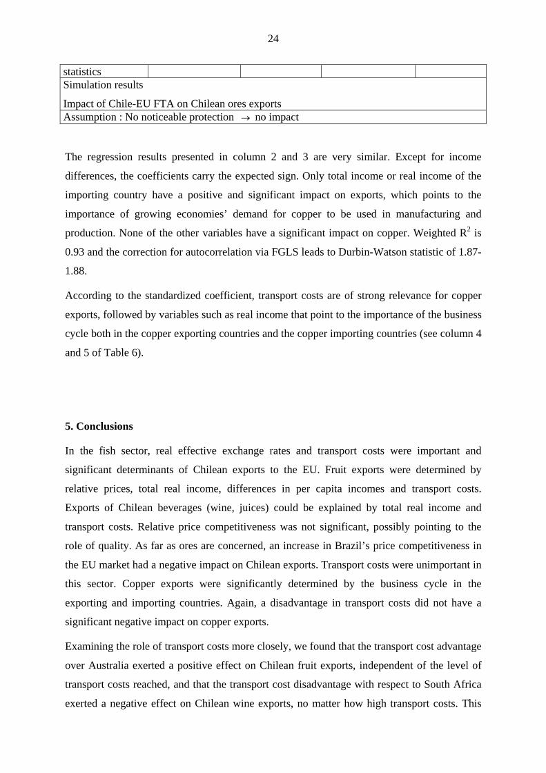
statistics Simulation results
Impact of Chile-EU FTA on Chilean ores exports Assumption : No noticeable protection → no impact
The regression results presented in column 2 and 3 are very similar. Except for income
differences, the coefficients carry the expected sign. Only total income or real income of the
importing country have a positive and significant impact on exports, which points to the
importance of growing economies’ demand for copper to be used in manufacturing and
production. None of the other variables have a significant impact on copper. Weighted R2 is
0.93 and the correction for autocorrelation via FGLS leads to Durbin-Watson statistic of 1.87-
1.88.
According to the standardized coefficient, transport costs are of strong relevance for copper
exports, followed by variables such as real income that point to the importance of the business
cycle both in the copper exporting countries and the copper importing countries (see column 4
and 5 of Table 6).
5. Conclusions
In the fish sector, real effective exchange rates and transport costs were important and
significant determinants of Chilean exports to the EU. Fruit exports were determined by
relative prices, total real income, differences in per capita incomes and transport costs.
Exports of Chilean beverages (wine, juices) could be explained by total real income and
transport costs. Relative price competitiveness was not significant, possibly pointing to the
role of quality. As far as ores are concerned, an increase in Brazil’s price competitiveness in
the EU market had a negative impact on Chilean exports. Transport costs were unimportant in
this sector. Copper exports were significantly determined by the business cycle in the
exporting and importing countries. Again, a disadvantage in transport costs did not have a
significant negative impact on copper exports.
Examining the role of transport costs more closely, we found that the transport cost advantage
over Australia exerted a positive effect on Chilean fruit exports, independent of the level of
transport costs reached, and that the transport cost disadvantage with respect to South Africa
exerted a negative effect on Chilean wine exports, no matter how high transport costs. This
25
finding points to a linear relationship between transport costs and exports in the fruit and
beverage sector. We found a non-linear relationship between transport costs and exports in the
fish sector, implying that transport costs cease to have a steadily increasing negative impact
on fish exports once they have reached a certain level. Our results point to the tremendous
importance of transport costs in the sectors agriculture and fishery. And in contrast to the
above-mentioned sectors, transport costs did not have a significant influence on ores or
copper exports.
The FTA between Chile and the EU is expected to have a noticeable, positive impact on fish,
fruit and beverages, but only once the transitional phase of the FTA has been completed. With
respect to an abolition of tariffs, fish exports would increase by 7.4% and fruit exports would
rise by 26.6% after a ten-year transitional phase. Exports of wine would shoot up by 21.3%
after a four-year transitional period.

26
References
Anderson, J. E. and E. Wincoop (2003), ‘Gravity with gravitas: a solution to the border
puzzle’, American Economic Review 93 (1), 170-192.
Anderson, J. E. and E. Wincoop (2004), ‘Trade costs’, Journal of Economic Literature 42 (3),
691-751.
Arnon, A., Spivak, A. and Weinblatt, J. (1996), 'The potential for trade between Israel, the
Palestinians and Jordan' , The World Economy 19: 113-134.
Bergstrand, J. H. (1985), 'The gravity equation in international trade: some microeconomic
foundations and empirical evidence', The Review of Economics and Statistics 67, 474-
481.
Bergstrand, J. H. (1989), ‘The generalised gravity equation, monopolistic competition, and the
factor-proportions theory in international trade’, The Review of Economics and Statistics
67, 474-481.
Bougheas et al. (1999), 'Infrastructure, transport costs and trade', Journal of International
Economics 47, 169-189.
Breuss, F. and Egger, P. (1999), ‘How reliable are estimations of East-West trade potentials
based on cross-section gravity analyses?’, Empirica 26 (2): 81-95.
Busse, M. (2003), ‘Tariffs, transport Costs and the WTO Doha Round: The case of
developing countries’, The Estey Centre Journal of International Law and Trade 4: 15-
31.
Chaire Mercosur-Science Po (2003), Annual Report 2002-2003,
http://chairemercosur.Science-po.fr/negotiations/rapport:annuel_2002_2003.pdf
(9 September 2005).
Chen, I-H. and H. J. Wall (1999), ‘Controlling for heterogeneity in gravity models of trade’,
Federal Reserve Bank of St. Louis Working Paper 99-010A.
Chumacero, R. A., R. Fuentues, and K. Schmidt-Hebbel (2004), ‘Chile’s free trade
agreements: How big is the deal?’ Central Bank of Chile Working Papers 264, Santiago,
Chile.
Egger, P. (2000), ‘A note on the proper econometric specification of the gravity equation’,
Economics Letters 66, 25-31.
Endoh, M. (2000),‘The transition of post-war Asia-Pacific trade relations’, Journal of Asian
Economics 10 (4): 571-589.
European Commission (2003), ‘Intra- and extra-EU trade, Annual data, Combined
Nomenclature, Supplement 2’, EUROSTAT, CD ROM of COMEXT trade data base.

27
European Parliament (2005), ‘Note on relations between Chile and the European Union’,
http://www.europarl.eu.int/meetdocs/2004_2009/documents/NT/552/55201/55201eu.pdf
(9 September 2005).
FERN, Greenpeace, WWF 2004 :
http://www.panda.org/news_facts/newsroom/news.cfm?uNewsID=17214 (28 July 2005).
Harrison, G.T., T. Rutherford, and D. Tarr (2003), Chile’s regional arrangements: The
importance of market access and lowering the tariff to six percent,’ Central Bank of Chile
Working Paper 238, Santiago, Chile.
Helpman, E. (1987), ‘Imperfect competition and international trade: evidence from fourteen
industrial countries’, Journal of the Japanese and International Economies 1 (1): 62-81.
Hufbauer, G. (1991), ‘World economic integration: The long view’ International Economic
Insights 2 (3): 26-27.
IDB (2001), The business of growth, Inter-American Development Bank, Washington, D. C.
2002 Japan Conference: A summary of the papers, NBER Website, Friday, July 29, 2005;
http://www.nber.org/2002japanconf/sutton.html (29 July 2005).
Limao, N. and A. J. Venables (2001), ‘Infrastructure, geographical disadvantage and transport
Costs’, World Bank Economic Review, 15 (3): 451-479.
Linder, S. B., An essay on trade and transformation, New York: Wiley & Sons, 1961.
Martínez-Zarzoso, I. and L. Márquez-Ramos (2004?), International trade, technological
innovation and income: A gravity model approach’, IN???
Martínez-Zarzoso, I. and F. Nowak-Lehmann D. (2003), ‘Augmented gravity model: An
empirical application to MERCOSUR-European Union trade flows’, Journal of Applied
Economics VI (2), 291-316.
Martínez-Zarzoso, I. and F. Nowak-Lehmann D. (2004), ‘Economic and geographical
distance: Explaining sectoral exports to the EU’, Open Economies Review 15 (3), 291-
314.
McPherson, M. A., M. R. Redfearn and M. A. Tieslau (2000), ‘A re-examination of the
Linder hypothesis: A random-effects Tobit approach’ International Economic Journal 14,
3, 123-136.
Mátyás, L. (1997), 'Proper econometric specification of the gravity model', The World
Economy 20 (3), 363-368.
OECD (1997), The Uruguay Round agreement on agriculture and processed agricultural
oroducts, OECD Publications, Paris.

28
SIA Chile-EU (2002), ‘Sustainable impact assessment of the trade aspects of negotiations of
an association agreement between the European Communities and Chile,’ Manuscript,
Planistat Luxembourg, Luxembourg.
Soloaga, I. and Winters, A. (1999), ‘Regionalism in the nineties: What effects on trade?’
Development Economic Group of the World Bank, mimeo.
Stock, J. H. and M. W. Watson (1993), ‘A simple estimator of cointegrating vectors in higher
order integrated systems’, Econometrica 61 (4), 783-820.
Supper, E. (2001), 'Is there effectively a level playing field for developing countries exports?',
UNCTAD, Policy Issues in International Trade and Commodities, Study Series No.1.
Wei, S.-J. (1996), ‘Intra-national versus international trade: how stubborn are nations in
global integration?’ NBER, Working Paper 5531.
Wines & Vines (2003), ‘Labeling ‘deal’ reported, News this month: January 2003,
http://www.findarticles.com/p/articles/mi.m3488/is_1_84/ai_97650933.
World Bank (2002), TradeCAN (Competeitiveness Analysis of Nations) 2002 CD-ROM,
Washington, D.C.
World Bank (2004), World Development Indicators, Data on CD ROM, Washington, D.C.
WTO Trade Policy Review, European Union (1995, 1997, 2000), World Trade Organisation,
Geneva.
WWF (World Wildlife Fund): EU imports of wood based products 2002 (2005):
http://www.panda.org/about_wwf/where we work/europe/problems/illegal_logging/ (29
April 2005)

29
Appendix
Description of Data
In the following, the variables presented in Tables 2-6 and equations (3a-b) : lxr, lyt, lydiff,
lreer, lreer* , ltcindex and ldtc* will be described in original form (not in logs). All data run
from 1988 to 2002.
In our case, six cross-sections (6 EU countries: Germany, Spain, France, UK, Italy, the
Netherlands) had overall complete time series.20
(1) Chilean exports to the EU or EU imports from Chile: xr
The export data x (in 1000 ECU) are taken from the COMEXT trade database of EUROSTAT
(Intra- and extra-EU trade, Annual data, Combined Nomenclature, Supplement 2, 2003). They
have been converted into real terms data (from the point of view of Chile) by considering
changes of the Chilean Peso exchange rate with respect to the ECU (EUR) and changes in the
Chilean price level (as measured by the GDP deflator of Chile).
(2) Total income of the trading pairs in PPP: yt
The yt data stem from the 2004 World Development Indicators CD-ROM. This variable
stands for PPP-income of Chile plus PPP-income of the relevant EU trading partner.
(3) Per capita income differences of the trading pairs in PPP: ydiff
The ydiff series is taken from the 2004 World Development Indicators CD-ROM. It is
computed as PPP-per capita income of relevant EU country minus PPP-per capita income of
Chile.
(4a) The Chilean real effective exchange rate: reer
reer is the bilateral real effective exchange rate between Chile and the EU countries (price
quotation system) from Chile’s perspective. It consists of the real exchange rate (rer) and
basic indicators of EU protection such as EU tariffs (t) and EU subsidies (s).
It is computed (all data for ‘rer’ are taken from World Development Indicators CD ROM of
2004) as:
rer = e ⋅ PEU/PChile with
rer = real bilateral exchange rate between Chile and relevant EU country
e = nominal exchange rate (x Chilean Peso/1EUR) between Chile and relevant EU country
PEU = GDP deflator of the EU country under consideration with 1995 as base year (1995 =̂
100)
20 Due to missing data, Austria, Belgium, Finland, Luxemburg and Sweden were excluded from the analysis.
30
PChile = GDP deflator of Chile with 1995 as base year (1995 =̂ 100)
rer has been adjusted for EU tariff protection (in terms of average EU tariff rate (t)) and non-
tariff protection (in terms of EU subsidy rate (s). Tariff rates prevailing in the EU can be
found in Trade Policy Review European Union, Volume 1, 2000, pp. 88-101 (WTO) and
rough subsidy equivalents are based on qualitative information on non-tariff protection
collected, explained and nicely presented for UNCTAD by Supper (2001).
So we get:
reer = rer ⋅ (1-s)/(1+t)
For the simulations, we assume that the FTA between Chile and the EU brings tariffs down to
zero.
(4b) Chile’s copper price in real terms: rpcopper
rpcopper = pcopper ⋅ eRCHUS/GDPDEFLRCH
with
pcopper = world market price of copper in US$ per ton
eRCHUS = nominal exchange rate Chilean Peso/US$ (price quotation system)
GDPDEFLRCH = Chilean GDP deflator
(5) Chile’s competitors real effective exchange rates :reer*
In analogy to (4) the real effective exchange rates of Chile’s main competitors Norway, South
Africa, Russia, Indonesia are computed. Nominal exchange rates, Norway’s, South Africa’s,
Russia’s and Indonesia’s GDP deflators are computed from World Development Indicators
CD ROM 2004. Tariff and subsidy rates are borrowed from WTO and UNCTAD (see (4)).
(6) Chile’s transport costs to main EU ports: tcindex
The transport cost index consists of two components: 1) the actual distance via available sea
routes (not great circle distance) between Chile and the EU country under consideration,
converted from nautical miles into km.21 Sea distance in km is widely regarded as appropriate
because sea transport costs one-fifth of land transport! 22 2) a freight cost index23 to be found
in Busse (2003) citing Hufbauer (1991), Figure 6: Transport and Communications Costs,
1930-2000 (in 1990 US$) that is extrapolated for the period of 1988 to 2002. Actual sea
distance is multiplied by the freight cost index with base year 2002.
tcindex = kmsea ⋅ fci
tcindex = transport cost (from Chile to relevant EU port)
21 http://www.maritimechain.com/port/port_distance.asp 22 This information was transmitted by fax on 17 August 2004 by the ShortSeaShipping Promotion Center, c/o Bundesverkehrsministerium für Verkehr, Bau- und Wohnungswesen (BMVBW Bonn ABTLG LS).
31
kmsea = sea distance in km of Chile to relevant EU port
fci = freight cost index with 2002 as base year (2002 =̂ 1)
(7) Transport cost differential between Chile and its main competitors: dtc
dtc measures differences in transport costs between Chile and Norway/South Africa etc. to the
EU market multiplied through with the freight cost index in the period of 1988 to 2002.
dtc* = (kmsea*-kmsea) ⋅ fci
dtc* = transport cost differential between Chile and extra-EU competitor *
kmsea* = sea distance in km of main extra-EU competitor (Norway, South Africa etc.) to
relevant EU port
kmsea = sea distance in km of Chile to relevant EU port
fci = freight cost index with 2002 as base year (2002 =̂ 1)
23 Average ocean freight and port charges per short ton of import and export cargo.