Ibero-Amerika Institut für Wirtschaftsforschung Instituto Ibero-Americano de Investigaciones Económicas

Ibero-America Institute for Economic Research (IAI)

Georg-August-Universität Göttingen

(founded in 1737)

Nr. 171

Aid and Trade – A Donor’s Perspective

Felicitas Nowak-Lehmann D., Inmaculada Martínez-Zarzoso, Stephan Klasen, Dierk Herzer

April 2008

Diskussionsbeiträge · Documentos de Trabajo · Discussion Papers

Platz der Göttinger Sieben 3 ⋅ 37073 Goettingen ⋅ Germany ⋅ Phone: +49-(0)551-398172 ⋅ Fax: +49-(0)551-398173

e-mail: uwia@gwdg.de ⋅ http://www.iai.wiwi.uni-goettingen.de

1

Aid and Trade—A Donor’s Perspective

Felicitas Nowak-Lehmann D.1 Inmaculada Martínez-Zarzoso2

Stephan Klasen3 Dierk Herzer4

Abstract

Foreign aid is given for a combination of economic, political, and humanitarian

motives. While its impact on economic development in recipient countries has been

the main focus of research recently, we concentrate on the question to what extent it

also promotes donor countries’ exports. We examine this issue using Germany as a

case study where the positive impact of aid on exports has been found to be extremely

high. Using more advanced methods, we compute an average return (between EUR

1.49 to EUR 1.72) of one EUR of aid spent, well below previous findings, but still

surprisingly large and robust.

Keywords: bilateral aid, donors’ exports, time series properties of panel data, ECM and

DOLS estimation in a panel context

JEL: F14, F35, C 23

1 Ibero-America Institute for Economic Research, University of Goettingen, Germany; e-mail: fnowak@gwdg.de, Ph. : + 49 551 397487 (contact) 2 University of Goettingen and University Jaume I, Castellón, Spain 3University of Goettingen, Germany 4 Wolfgang-Johann Goethe University, Frankfurt, Germany

2

Acknowledgements We would like to thank Jutta Albrecht, Mario Larch, Adolf Kloke-Lesch, Rigmar Osterkamp,

and Klaus Wardenbach for helpful comments and discussion. Funding from the German

Ministry of Economic Cooperation and Development and from Projects Caja Castellón-

Bancaja:P1-1B2005-33 and SEJ2007-67548 in support of this work are gratefully

acknowledged.

3

Aid and Trade—A Donor’s Perspective

1. Introduction

The primary objective of German bilateral foreign aid5 is to contribute to efforts to overcome

worldwide poverty, underdevelopment, and distress. Nonetheless, German development

agencies and the German taxpayer are also interested in learning about the impact of aid on

Germany’s economy. The investigation of this issue is even more important as the German

government is not only willing, but even obliged under an EU agreement to noticeably

increase its official development aid in the years to come. The EU agreement aims to fulfill

the UN goal of 0.7 per cent in the year 2015 (rich countries should spend at least 0.7 per cent

of their GNP on official development aid [ODA]). This would imply for Germany that 0.5 per

cent of German GNP should be spent on development aid in 2010. Currently, the German

government spends 0.35 per cent of its GNP on ODA (9 billion US$) implying that German

ODA will have to increase substantially over the next eight years.

In 1999, a study investigated the impact of German bilateral aid on German exports.

Amazingly, they found, based on 1976-to-1995 data, that one Deutschmark spent on bilateral

ODA would increase export revenues by 4.3 marks; this effect was quite unrelated to the

practice of tying aid to exports and was, in any case, much larger than the aid flow, itself

Since this figure appears remarkably high, this paper re-examines these findings for Germany

based on 1962-to-2005 data to get a clearer understanding of the impact of Germany’s

bilateral aid on German export revenues. This study uses a more complex model and more

modern estimation techniques compared to most other studies in this literature, including the

previous estimation. It differs from earlier ‘aid and trade’ studies in two respects: First,

compared to the 1999 study, it utilises a set of control variables that are indispensable for

5 In the following we will call it just aid.

4

obtaining plausible and reliable results. Second, it takes the time-series properties of the

analysed data into account, thus avoiding the problem of spurious correlations in non-

stationary data6.

The organisation of the paper is as follows: In Chapter 2 an overview of the aid and trade

literature will be given. Chapter 3 contains the econometric model and the estimation

techniques. In Chapter 4 the empirical results are presented and Chapter 5 concludes.

2. Overview of Related Literature

In recent decades, a great research effort has been devoted to investigating the effects of

developmental assistance on the economic performance of the recipient countries (for

example, Burnside and Dollar, 2000) and to clarify the recent debate on ‘aid for trade’

(Morrisey, 2006). Very little attention has been devoted to the reverse issue of quantifying the

impact of aid on donors’ export revenues. While this is not (and should not be) the main

motivation for giving aid, it would nevertheless be worthwhile to examine this. A finding that

aid flows promote exports would suggest that giving aid (if it also promotes development in

the recipient country) can be a ‘win-win’ situation for both parties and might also reduce

taxpayer reluctance to devote resources to aid.

The Arvin and Baum (1997) and Arvin and Choudry (1997) studies evaluated the relationship

between bilateral aid and bilateral exports with and without tying of the aid to donors’

contracts of sale. They showed that aid without tying was roughly as export-promoting as tied

aid. They explained this phenomenon by the effects of the recipient countries’ good will

and/or parallel trade agreements and trade concessions. On these grounds, a formal tying of

aid is no longer recommendable (Jepma, 1991; Arvin and Baum, 1997; Arvin and Choudry,

1997). Benefits for donors through tying are usually insubstantial, whereas tying noticeably

reduces the benefit of aid for recipients (Jepma, 1991; Wagner, 2003). Consequently, tying 6 Driven by pure correlations over time.

5

has been stepwise reduced, partly due to pressure from the Development Assistance

Committee [DAC].

The relationship between aid and exports was examined in various country studies which

neglect, however, the possible occurrence of spurious regressions.7 Therefore, a word of

caution is needed regarding the results, since the figures have been derived from trending

series. Non-stationarity of the series and/or autocorrelation of the disturbances have not been

(sufficiently) taken into account even though some studies’ authors tried to reduce

spuriousness in the regressions by averaging over time and plugging in a time trend, or by

utilising data in five-year intervals.

Vogler et al. (1999) found that one mark spent on ODA would increase exports by 4.3 marks,

using data for the period 1976 to 1995 for Germany’s aid and trade relationship. The authors

included 43 recipient countries in the study but the average impact of aid on trade was

calculated for only 23 of those countries. A study done by Nilsson (1997) on the aid and trade

relationship of EU countries and developing countries showed that one US dollar’s worth of

aid increased exports by $2.60 (the average for EU countries) and by $3.20 (figure for

Germany). The period of study ran from 1975 to 1992. The author utilised a common

intercept for all the EU countries, three-year averages, and a time trend. Studying the aid and

trade relationship between OECD donors (especially Japan) and recipient countries, Wagner

(2003) computed the impact of one US dollar of aid to be approximately $2.30, utilising

pooled data for the years 1970, 1975, 1980, 1985, and 1990 to minimise distortions from

autocorrelation.8

A totally different approach was followed by Lloyd, McGillivray, Morissey, and Osei (2000),

Arvin, Cater, and Choudry (2000), and Osei, Morissey, and Lloyd (2004). The authors tested

7 Spurious regression results occur when either autocorrelation of the disturbances is not taken into account or regressions with non-stationary series are run. Autocorrelation and non-stationarity of the series are interlinked, as they result from memory of the series. 8 This procedure may reduce autocorrelation, but is unable to eliminate it. In the presence of autocorrelation, the residuals in 1990 will still be correlated with the residuals of 1985 and earlier years.

6

Granger causality and cointegration9, getting mixed results for the aid and trade relationship.

For some country pairs the authors could not find an aid-trade link, for other country pairs the

aid-trade link existed, and for still others, they could identify a bi-directional relationship.

This bi-directional relationship eventually led us to control for possible endogeneity of the aid

variable.

Finally, a few of the studies which focused on quantifying the impact of the donors’ aid on

trade utilised the gravity model of trade (Nilsson 1997; Wagner, 2003). We also believe that

the gravity model is well suited to study the impact of aid on trade since it allows controlling

for the impact of regular factors on trade such as income (production capacity and income

variety effect), population (absorption and economies of scale effect), and distance in a world

where trade agreements, exchange rates, and aid can also influence trade.

We deviate from most of those studies by exploiting the time-series properties of the series in

a more appropriate manner. We find that a superficial analysis or neglect of the time-series

properties changes the regression results substantially. Therefore, we do control for trends and

memory in the series, thus avoiding spurious regression result; utilising the study period from

1962 to 2005 allows us to do so. In addition, we can distinguish between the short-term and

the long-term impact of aid and trade by applying a fully dynamic error correction model

[ECM]. We also control for the endogeneity of aid by estimating the aid-export relationship

with Dynamic Ordinary Least Squares [DOLS] and Dynamic Feasible Generalized Least

Squares [DFGLS].

This study also differs from a preceding study done by our research group which uses

Germany as a case study and utilises the same original data set as this study. Whereas the pre-

study (or companion study) tries to improve and update the estimation methods for the

standard static and dynamic ‘aid and trade’ models?10, this paper models the dynamics in a

9 The requirement for testing cointegration, that all variables must be integrated of the same order, (in other words,, I(1) or I(p)), was not fulfilled with respect to the majority of the countries examined. 10 This is the Koyck lag model, also called the autoregressive distributed lag model (ARDL).

7

different way and gives serious consideration to the time series approach to panel regressions.

Furthermore, we exclusively look at countries that have an established co-operation treaty

with Germany making them the most important recipients of German aid11, whereas the

companion paper concentrates on finding the aid-and-trade relationship for all developing

countries with available data and the most important sub-groups of that data. The subdivision

of the sample in the companion paper aims at determining whether various countries

demonstrate different degrees of goodwill towards Germany as donor country. The

companion study is not, however, about whether aid-tying conditions differ among country

groups given that Germany’s aid-donation level ranks below average in total amount

compared to other EU countries since (only seven per cent of Germany’s ODA was tied in

2005).

3. Model and Estimation Techniques

3.1 Modelling the Aid-Trade Link

In this paper, we focus exclusively on the effect of aid on the donor’s exports. Analogous to

the welfare implications of bilateral transfers for donor and recipient countries, which were

debated by Keynes (1929), Ohlin (1929), and Djajic, Lahiri, and Raimondos-Moller (2004),

and nicely summarised by Lahiri (2005), we expect that, in the context of an intertemporal

model of trade, development aid will lead to an increase in the donor’s exports mainly due to

the presence of habit formation or goodwill effects. In the presence of habit-formation effects,

aid given today shifts preferences of the recipient in favour of the donor’s export goods in the

future. In order to evaluate this effect empirically, we have chosen the gravity model of trade

as a basic framework.

11 A complete list of these so-called BMZ countries can be found in the appendix.

8

The gravity model is currently the most commonly accepted framework for modelling

bilateral trade flows. According to the underlying theory, trade between two countries is

explained by the nominal incomes and the populations of the trading countries, the distance

between the economic centres of the exporter and importer, and by a number of other factors

aiding or hindering trade (colonial history, common language, and so on.) between them. In

1979, Anderson provided a theoretical foundation for the gravity equation based on the

concept of product differentiation in the American Economic Review. Our version of the

gravity model goes back to Bergstrand (1985), who derived the gravity model from a general

equilibrium model of trade. If trade flows are perfect substitutes for one another and not

differentiated by origin, then the gravity model functions correctly without a price term, as in

Equation 1, below. Under realistic assumptions, however, a price term must be added to

avoid misspecification (see Equation 2, below). This price term takes care of the imperfect

substitutability of trade flows and/or large and persistent deviations in national price levels

from purchasing power parity [PPP]. The bilateral exchange rate can be used as a proxy for

prices.

According to the original gravity model of trade, the volume of exports between pairs of

countries, Xij, is a function of their income ( ji YY , ), their populations ),( ji POPPOP , their

geographical distance from one another, )( ijDIST , and a set of dummies )( ijF :

ijijijjijiij uFDISTPOPPOPYYX 6543210

ααααααα= . (1)

In line with Bergstrand, Equation 1 was augmented to accommodate the role played by

exchange rates, our proxy for prices. Income transfers, namely bilateral and multilateral aid,

are added, as well, giving us

9

ijijijijijijjijiij uFDISTEUAIDGBAIDGEXRNPOPPOPYYX 9876543210

αααααααααα= . (2)

Equation 2 is a reduced form of a partial equilibrium subsystem of a general equilibrium trade

model with nationally differentiated products. Yi (Yj) indicates the GDPs of the exporter

(importer), POPi (POPj) are exporter (importer) populations, ijEXRN stands for the bilateral

exchange rate between countries i and j, ijBAIDG measures the amount of gross bilateral aid

going from Germany to developing country j, ijEUAIDG measures the amount of gross EU

aid that is given to developing countries, DISTij measures the distance between the two

countries’ capitals (or economic centres), and Fij represents all other factors aiding or

preventing trade between pairs of countries, such as adjacency, language, isolation (such as

for islands), or belonging to a certain trading bloc. uij is the error term.

Since we will work in the fixed effects framework12, all factors that are cross-section specific

and do not vary over time (distance, adjacency, language, island), will interfere with the

cross-section-specific intercepts and cannot be directly estimated. These factors thus lead to

ijijijijjijiijij uEUAIDGBAIDGEXRNPOPPOPYYX 654321)( βββββββ= . (3)

This model is usually linearised13 and then estimated in its log-log form,

12 The Hausman test rejected the random-effect model due to correlation between the random-country effect and the error term. 13 Santos Silva and Tenreyro (2006) suggested estimating the non-linear model with the Pseudo Poisson Maximum Likelihood technique [PPML] pointing to Jensen’s inequality (a problem linked to the error term that arises in the linearisation process) and a better ability to deal with heteroskedasticity. However, empirical applications of the PPML technique to real trade data were less promising. Heteroskedasticity remained a problem and the model assumptions proved.difficult to fulfill.

10

ijtijtijt

ijtjtitjtitijijt

uEUAIDGBAIDG

EXRNPOPPOPYYX

+++

++++=

lnln

lnlnlnlnln

65

4321

ββ

ββββµ

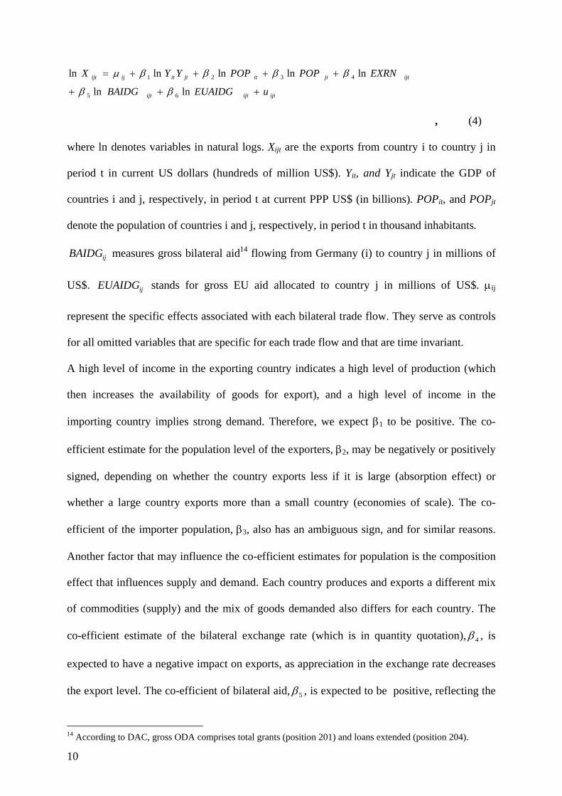
, (4)

where ln denotes variables in natural logs. Xijt are the exports from country i to country j in

period t in current US dollars (hundreds of million US$). Yit, and Yjt indicate the GDP of

countries i and j, respectively, in period t at current PPP US$ (in billions). POPit, and POPjt

denote the population of countries i and j, respectively, in period t in thousand inhabitants.

ijBAIDG measures gross bilateral aid14 flowing from Germany (i) to country j in millions of

US$. ijEUAIDG stands for gross EU aid allocated to country j in millions of US$. µij

represent the specific effects associated with each bilateral trade flow. They serve as controls

for all omitted variables that are specific for each trade flow and that are time invariant.

A high level of income in the exporting country indicates a high level of production (which

then increases the availability of goods for export), and a high level of income in the

importing country implies strong demand. Therefore, we expect β1 to be positive. The co-

efficient estimate for the population level of the exporters, β2, may be negatively or positively

signed, depending on whether the country exports less if it is large (absorption effect) or

whether a large country exports more than a small country (economies of scale). The co-

efficient of the importer population, β3, also has an ambiguous sign, and for similar reasons.

Another factor that may influence the co-efficient estimates for population is the composition

effect that influences supply and demand. Each country produces and exports a different mix

of commodities (supply) and the mix of goods demanded also differs for each country. The

co-efficient estimate of the bilateral exchange rate (which is in quantity quotation), 4β , is

expected to have a negative impact on exports, as appreciation in the exchange rate decreases

the export level. The co-efficient of bilateral aid, 5β , is expected to be positive, reflecting the

14 According to DAC, gross ODA comprises total grants (position 201) and loans extended (position 204).

11

income-transfer effect of aid. The co-efficient of multilateral aid, 6β , can be either positive or

negative depending on whether the recipient countries prefer to import from known channels

or instead choose to diversify their import channels.

Equation 4 represents the static model, which model allows conclusions for the long-term

equilibrium to be drawn. Use of this model, however, can lead to spurious regression results

when the variables substituted into it reflect a deterministic or stochastic time trend.

Estimating Equation 4 with pooled least squares and fixed effects results in an R2 of 0.96 and

a Durbin-Watson statistic [DW] of 0.54, which is remote from the ideal of 2.00. As R2

exceeds the DW, we have an indication of a spurious relationship and of spurious regression

co-efficients.

12

3.2 Data Sources, Variables, and German Co-operation Countries

Official Development Aid data are from the OECD Development Database on Aid from DAC

members15. Bilateral exports are obtained from the UN COMTRADE database. Data on

income and population variables are drawn from the World Bank (World Development

Indicators Database 2006). Bilateral effective exchange rates are from the IMF statistics.

Distances between capitals have been computed as great circle distances using data on

straight-line distances in kilometres; latitudes and longitudes were obtained from the CIA

World Fact Book.

In the Appendix, A.2 is a list of partner countries of German Development Co-operation

(BMZ countries). See also http://www.bmz.de/en/countries/laenderkonzentration/tabelle.html.

These countries will be the main focus of the analysis, as the BMZ has a bilateral aid

relationship only with them.16

3.3 Estimation Issues

Since spurious correlations are to be avoided, alternative estimation methods will rely on an

error correction model [ECM] or a long-run model with built-in leads and lags to control for

endogeneity of the explanatory variables. Error correction models allow one to draw

inferences that are not driven by spuriousness. All a priori stationary variables are excluded

from the ECM as they do not contribute to the long-term equilibrium. Only if the series is

integrated to the same order and co-integrated in the long-term (such that the residual of

Equation 4 is stationary) can these variables enter the model. Stock (1987) and Pesaran et al.

15 www.oecd.org/dac/stats/idsonline. 16 Other developing countries might also receive German development assistance that is provided via NGOs, disaster relief, scholarships for students from these countries, or funding for foundations active in these countries. We would not expect that these aid flows much affect exports from Germany.

13

(2001) suggested using an ECM based on an ARDL17, leading to a dynamic error correction

model.

The dynamic error correction model is given by

ijtijtijtijtjt

itjtitijtkp

p pijtp

tpijpkp

ppijtpkp

ppijtpkp

p

pjtpkp

ppitpkp

ppjtpitpkp

pijijt

uEUAIDGbBAIDGbEXRNbPOPb

POPbYYbXX

EUAIDGBAIDGEXRN

POPPOPYYX

+−−−−

−−⋅+∆

+∆+∆+∆

+∆+∆+∆+=∆

−−−−

−−−−=

= −

−=

=−=

=−=

=

−=

=−=

=−−=

=

∑∑∑∑

∑∑∑

)lnlnlnln

lnln(lnln

lnlnln

lnlnlnln

16151413

1211111

605040

302010

λλ

βββ

βββµ

(5)

Both short-term ( pp 61 ,...,ββ ) and long-term co-efficients ( 61,...,bb ) can be estimated. λ

describes the adjustment to the long-term equilibrium. The term

)lnlnlnlnlnln(ln 16151413121111 −−−−−−−− −−−−−− ijtijtijtjtitjtitijt EUAIDGbBAIDGbEXRNbPOPbPOPbYYbX

is the error-correction term and contains the long-term elasticities. The short-run relationship

is described by the variables in differences18, thereby removing their stochastic trend (Hendry,

1995; Mukherjee et al., 1998).

The maximum lag length, k, is determined by the Schwarz criterion. In our case, k is equal to

three. Hendry’s (1995) general-to-specific method is applied to Equation 6, thus eliminating

the least significant variables. We end up with the following ARDL-based ECM:

ijtijtijtijtjt

itjtitijtp

p pijtp

ijtijtijtijt

itjtitjtitijijt

uEUAIDGbBAIDGbEXRNbPOPb

POPbYYbXX

EUAIDGBAIDGEXRNEXRN

POPYYYYX

+−−−−

−−⋅+∆

+∆+∆+∆+∆

+∆+∆+∆+=∆

−−−−

−−−−=

= −

−−

−−

∑)lnlnlnln

lnln(lnln

lnlnlnln

lnlnlnln

16151413

1211113

1

1615034340

20111110

λλ

ββββ

βββµ

(6)

17 Irrespective of whether the regressors are I(0) or I(1), an ARDL can be applied. Pesaran et al. compute the critical values for a cointegration test in the ARDL framework for time series (Pesaran et al.,_2001). 18∆ means that the variables enter the model in first differences.

14

However, an increase in the amount of donors’ exports resulting from aid given might make it

more attractive to the recipient country to give more bilateral aid in turn. Trade can lead to

further aid if donors preferably allocate their aid to countries with which they have the

greatest commercial links. Since it is therefore debatable whether the variable, ln BAIDG, is

truly exogeneous, a control for possible endogeneity is called for. Where endogeneity

problems arise, estimation of the gravity model by the means of Dynamic Ordinary Least

Squares [DOLS] is recommended. DOLS is based on a modified version of Equation 4 that

includes past, present, and future values of the change in the regressors (Stock and Watson,

1993, 2003). When estimating Equation 7,

ijtkp

kp ijtpijtkp

kp pijtkp

kp pjtkp

kp p

itkp

kp pjtitkp

kp pijtijt

ijtjtitjtitijijt

uEUAIDGBAIDGEXRNPOP

POPYYEUAIDGBAIDG

EXRNPOPPOPYYX

∑∑∑∑∑∑

+=

−=

+=

−=

+=

−=

+=

−=

+=

−=

+=

−=

+∆+∆+∆+∆

+∆+∆+++

++++=

lnlnlnln

lnlnlnln

lnlnlnlnln

65

4321

ηγϕφ

εδχχ

χχχχα

(7)

consistent regression co-efficients can be obtained. In this case, the Schwarz criterion

suggested taking two leads and two lags (k=2).

If the dependent variable and the regressors are co-integrated, which co-integration must be

tested beforehand, then the DOLS estimator is efficient in large samples. Moreover, statistical

inferences about the co-integration co-efficients, 61 ,...,χχ , and the co-efficients

pppppp ηγϕφεδ ,,,,, in Equation 7, based on HAC standard errors, are valid. This is because

the t-statistic constructed using the DOLS estimator with HAC standard errors has a standard

normal distribution in large samples. And if the regressors were strictly exogenous, the co-

efficients, 61 ,...,χχ , in Equation 7, would be the long-term cumulative multipliers, that is, the

long-term effect on exports of a change in the explanatory variables. If the regressors are not

strictly exogenous, then the co-efficients are not given this interpretation.

15

3.4 Requirements for Non-Spurious Estimation

The dynamic ECM requires the change variables to be integrated of the same order (for

example, I(1)) and to have a long-run relationship (such that the long-run relationship has to

be stationary (I(0)).

Table 1 shows the test results for the variables. After inspecting the graphs, an intercept and

trend were assumed and a lag length of four was chosen. According to the ADF-Fisher Chi-

Square test, which allows for individual unit roots, all variables that enter the regression

model are I(1).

Table 1: Results from the ADF-Fisher Panel Unit Root Test

Variable tested

Null hypothesis

Unit root test utilised

Probability Observations Variable is integrated

Lx Individual unit root process

ADF-Fisher Chi-square 142.79

0.33 2279 I(1)

Lyy Individual unit root process

ADF-Fisher Chi-square 72.10

1.00 2198 I(1)

Lpopg Unit root process

ADF test statistic 86.34

1.00 2847 I(1)

Lpopj Individual unit root process

ADF-Fisher Chi-square 92.60

1.00 2831 I(1)

Lexrn Individual unit root process

ADF-Fisher Chi-square 96.19

0.97 2185 I(1)

Lbaidg Individual unit root process

ADF-Fisher Chi-square 89.04

0.99 2210 I(1)

Leuaidg Individual unit root process

ADF-Fisher Chi-square 141.55

0.27 2282 I(1)

16

However, words of caution are required. Clearly, unit root tests that assume individual unit

roots (for each cross-section)19 are to be preferred over unit root tests that assume a common

unit root process20, given that the first ones are much more flexible. Nonetheless, the available

panel unit root tests can lead to implausible results, especially when the number of cross-

sections is large. Cross-section correlation of the series is controlled best by the ADF-Fisher

panel unit root test (Maddala and Wu, 1999). For example, as to the aid and trade data

utilised, we know from the unit root test results at the country level (pure time series Phillips-

Perron Fisher unit root test, the ADF test, and the Im, Pesaran, and Shin test) that our series

are non-stationary (integrated of order 1, I(1) variables) in the vast majority of countries. In

our experience, the ADF-Fisher unit root test best reproduced the results obtained on an

individual level, whereas the PP-Fisher unit root test concludes far too often that the series are

stationary when they are, in fact, non-stationary on a country level (an individual level). The

results of the Im, Pesaran, Shin (IPS) test lie somewhere in between the ADF-Fisher and the

PP-Fisher unit root tests. These varying results have to do with the way the null and the

alternative hypotheses are formulated.21 In the alternative hypothesis, statements are made on

whether either all or a significant portion of the cross-sections is stationary.

When testing for co-integration, that is to say, the existence of a long-run relationship in the

aid and trade equation, we follow residual-based co-integration tests (Kao, 1999). The idea of

a residual-based co-integration test goes back to Engle and Granger (1987), who applied it to

time series. As to regressions with time series, if the residual (ut) of a regression is built

around variables with the same order p of integration (in other words, the variables ~ I(p) are

stationary, such that ut ~ I(0)), it is said that the I(p) variables are co-integrated, and therefore

a long-run relationship does exist. However, these tests not only tend to suffer from

19 Such as the Im, Pesaran, and Shin unit root test, the ADF- Fisher Chi-Square unit root test, and the PP-Fisher Chi-Square unit root test. 20 Such as the Levin, Lin, and Chu unit root test and the Breitung unit root test. 21 H0: All of the individuals of the panel have a unit root (the series has a unit root in all cross-sections); H1: The series is stationary in all cross-sections or according to the IPS test, H0: The series has a unit-root in all cross-sections, H1: Some, but not all, of the fractions of the individuals are (trend) stationary.

17

unacceptably low power when applied to series of moderate length, but also require special

critical values (for example, Kapetanios’s critical values)22 to test for stationarity of the

residuals (Kapetanios, 1999).

Pooling data across individual members of a panel when testing for co-integration is therefore

advantageous. Pooling increases the power of the unit root test by providing considerably

more information regarding the co-integration hypothesis23. But testing for co-integration in a

panel setting is also more complicated since two types of co-integration can be present and

must be taken into account: first, between series over time (the type prevailing in time series)

and second, between cross sections24 (the type potentially existing in a panel setting)

(Banerjee et al., 2004; Breitung and Pesaran, 2005; Urbain and Westerlund, 2006). We choose

Pedroni’s panel co-integration test which belongs to the single equation approaches25

(Pedroni, 1999, 2004). It involves estimating the hypothesised co-integrating regression

separately for each country (73 countries) and then testing the estimated residuals for

stationarity with adequate critical values using seven test statistics. Four of these statistics

pool the autoregressive co-efficients across different countries while performing the unit root

test and thus restrict the first order autoregressive parameter to being the same for all

countries. Pedroni (1999) refers to these statistics as panel co-integration statistics. The other

three statistics are based on averaging the individually estimated autoregressive co-efficients

for each country. Accordingly, these statistics allow the autoregressive coefficient to vary

across countries and are referred to as group mean panel co-integration statistics. Both panel

22MacKinnon’s critical values cannot be used when testing the non-stationarity of residuals. In this case, adjustments for the number of regressors in the regression equation are necessary and different critical values result. 23 H0: The variables of interest are not co-integrated for each member of the panel and H1; For each member of the panel, there exists a single co-integrating vector, although this co-integrating vector does not have to be the same for each member (Pedroni, 1999). 24Cross-sectional correlation can be addressed by the Seemingly Unrelated Regression (SUR) technique, but only if T is large and substantially larger than N, (N must be quite small). In our case, SUR would not work. Westerlund (2007a, 2007b, and 2007c) develops a more general solution to cross-unit correlation. He allows for cross-sectional dependence by assuming that the correlation can be modelled using a common factor structure. 25 It also belongs to the first generation panel co-integration tests. The first generation panel co-integration tests assume cross-sectionally-independent panels (Wagner and Hlouskova, 2007).

18

co-integration statistics and the group mean panel co-integration statistics test the null

hypothesis H0: ‘All of the individuals of the panel are not co-integrated.’ For the panel

statistics, the alternative hypothesis is H1: ‘All of the individuals of the panel are co-

integrated’, while for the group mean panel statistics, the alternative is H1: ‘A significant

portion of the panel members are co-integrated’ (Pedroni, 2004).

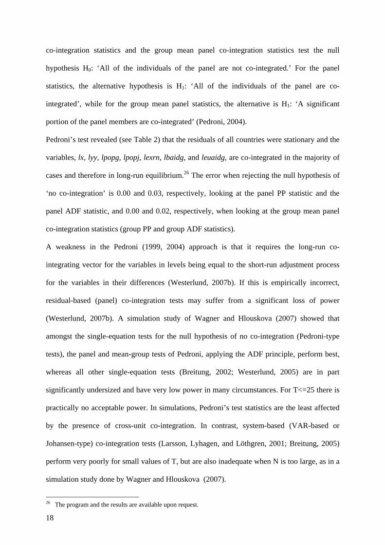
Pedroni’s test revealed (see Table 2) that the residuals of all countries were stationary and the

variables, lx, lyy, lpopg, lpopj, lexrn, lbaidg, and leuaidg, are co-integrated in the majority of

cases and therefore in long-run equilibrium.26 The error when rejecting the null hypothesis of

‘no co-integration’ is 0.00 and 0.03, respectively, looking at the panel PP statistic and the

panel ADF statistic, and 0.00 and 0.02, respectively, when looking at the group mean panel

co-integration statistics (group PP and group ADF statistics).

A weakness in the Pedroni (1999, 2004) approach is that it requires the long-run co-

integrating vector for the variables in levels being equal to the short-run adjustment process

for the variables in their differences (Westerlund, 2007b). If this is empirically incorrect,

residual-based (panel) co-integration tests may suffer from a significant loss of power

(Westerlund, 2007b). A simulation study of Wagner and Hlouskova (2007) showed that

amongst the single-equation tests for the null hypothesis of no co-integration (Pedroni-type

tests), the panel and mean-group tests of Pedroni, applying the ADF principle, perform best,

whereas all other single-equation tests (Breitung, 2002; Westerlund, 2005) are in part

significantly undersized and have very low power in many circumstances. For T<=25 there is

practically no acceptable power. In simulations, Pedroni’s test statistics are the least affected

by the presence of cross-unit co-integration. In contrast, system-based (VAR-based or

Johansen-type) co-integration tests (Larsson, Lyhagen, and Löthgren, 2001; Breitung, 2005)

perform very poorly for small values of T, but are also inadequate when N is too large, as in a

simulation study done by Wagner and Hlouskova (2007).

26 The program and the results are available upon request.

19

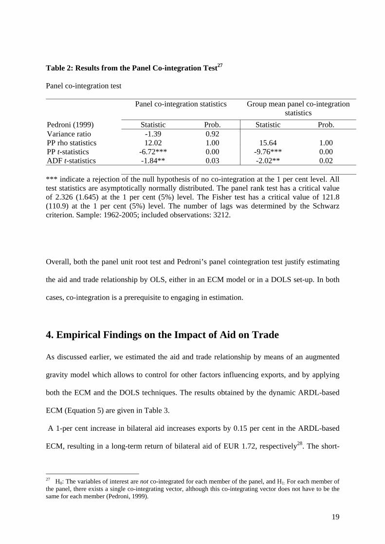
Table 2: Results from the Panel Co-integration Test27

Panel co-integration test

Panel co-integration statistics Group mean panel co-integration statistics

Pedroni (1999) Statistic Prob. Statistic Prob. Variance ratio -1.39 0.92 PP rho statistics 12.02 1.00 15.64 1.00 PP t-statistics -6.72*** 0.00 -9.76*** 0.00 ADF t-statistics -1.84** 0.03 -2.02** 0.02 *** indicate a rejection of the null hypothesis of no co-integration at the 1 per cent level. All test statistics are asymptotically normally distributed. The panel rank test has a critical value of 2.326 (1.645) at the 1 per cent (5%) level. The Fisher test has a critical value of 121.8 (110.9) at the 1 per cent (5%) level. The number of lags was determined by the Schwarz criterion. Sample: 1962-2005; included observations: 3212.

Overall, both the panel unit root test and Pedroni’s panel cointegration test justify estimating

the aid and trade relationship by OLS, either in an ECM model or in a DOLS set-up. In both

cases, co-integration is a prerequisite to engaging in estimation.

4. Empirical Findings on the Impact of Aid on Trade

As discussed earlier, we estimated the aid and trade relationship by means of an augmented

gravity model which allows to control for other factors influencing exports, and by applying

both the ECM and the DOLS techniques. The results obtained by the dynamic ARDL-based

ECM (Equation 5) are given in Table 3.

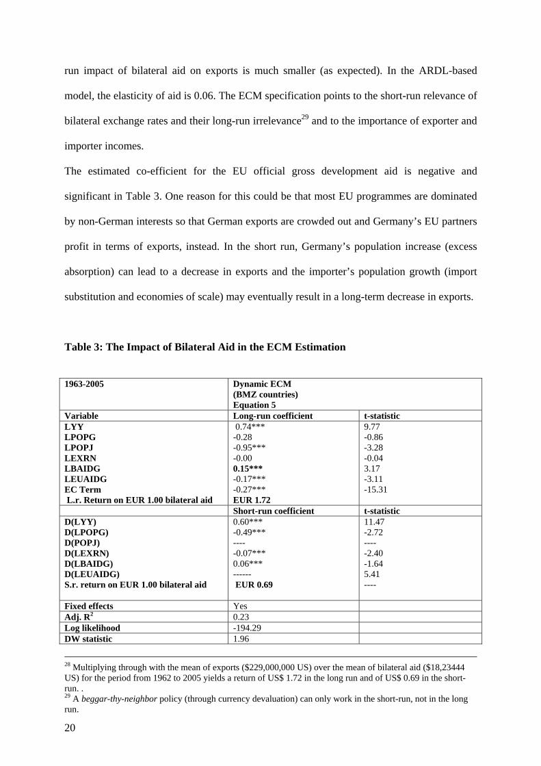
A 1-per cent increase in bilateral aid increases exports by 0.15 per cent in the ARDL-based

ECM, resulting in a long-term return of bilateral aid of EUR 1.72, respectively28. The short-

27 H0: The variables of interest are not co-integrated for each member of the panel, and H1: For each member of the panel, there exists a single co-integrating vector, although this co-integrating vector does not have to be the same for each member (Pedroni, 1999).

20

run impact of bilateral aid on exports is much smaller (as expected). In the ARDL-based

model, the elasticity of aid is 0.06. The ECM specification points to the short-run relevance of

bilateral exchange rates and their long-run irrelevance29 and to the importance of exporter and

importer incomes.

The estimated co-efficient for the EU official gross development aid is negative and

significant in Table 3. One reason for this could be that most EU programmes are dominated

by non-German interests so that German exports are crowded out and Germany’s EU partners

profit in terms of exports, instead. In the short run, Germany’s population increase (excess

absorption) can lead to a decrease in exports and the importer’s population growth (import

substitution and economies of scale) may eventually result in a long-term decrease in exports.

Table 3: The Impact of Bilateral Aid in the ECM Estimation

1963-2005 Dynamic ECM

(BMZ countries) Equation 5

Variable Long-run coefficient t-statistic LYY LPOPG LPOPJ LEXRN LBAIDG LEUAIDG EC Term L.r. Return on EUR 1.00 bilateral aid

0.74*** -0.28 -0.95*** -0.00 0.15*** -0.17*** -0.27*** EUR 1.72

9.77 -0.86 -3.28 -0.04 3.17 -3.11 -15.31

Short-run coefficient t-statistic D(LYY) D(LPOPG) D(POPJ) D(LEXRN) D(LBAIDG) D(LEUAIDG) S.r. return on EUR 1.00 bilateral aid

0.60*** -0.49*** ---- -0.07*** 0.06*** ------ EUR 0.69

11.47 -2.72 ---- -2.40 -1.64 5.41 ----

Fixed effects Yes Adj. R2 0.23 Log likelihood -194.29 DW statistic 1.96

28 Multiplying through with the mean of exports ($229,000,000 US) over the mean of bilateral aid ($18,23444 US) for the period from 1962 to 2005 yields a return of US$ 1.72 in the long run and of US$ 0.69 in the short-run. . 29 A beggar-thy-neighbor policy (through currency devaluation) can only work in the short-run, not in the long run.

21

F-statistic 7.82 Prob(f-stat) 0.00

Table 4 presents the results that are obtained by means of a DOLS estimation. First, we

estimate a regular DOLS30 (Equation 7) and then a DFGLS (Dynamic Feasible Generalized

Least Squares), controlling for autocorrelation31.

Table 4: The Impact of Bilateral Aid in the DOLS Estimation

1965-2003 DOLS

(BMZ countries)

Equation 7

DFGLS (correction of autocorrelation)

(BMZ countries)

Equation 7

Variable Long-run coeff. t-statistic Long-run coeff. t-statistic

LYY LPOPG LPOPJ LEXRN LBAIDG LEUAIDG L.r. return on

bilateral aid

0.87*** -0.53*** -1.18*** -0.04*** 0.19*** -0.24*** EUR 2.18

37.77 -3.13 -8.99 -4.37 7.34 -9.31

0.82*** -0.43 -1.32*** -0.04*** 0.13*** -0.08 EUR 1.49

16.64 -1.44 -5.12 -2.14 2.88 -1.41

2 leads and 2 lags

Yes Yes

Fixed effects Yes Yes

Adj. R2 0.96 0.98

Log likelihood -842.50 -158.08

DW Statistic 0.62 2.01

F -statistic 409.60 786.69

Prob (F-stat.) 0.00 0.00

The results obtained by estimating Equation 7 with and without controlling for autocorrelation

are rather similar. Control for autocorrelation is based on the Cochrane-Orcutt procedure in

30 Not reporting the short-run co-efficients. 31 Not reporting the short-run co-efficients.

22

which the correlation co-efficient, ρ , of the disturbances is estimated in the first step. Then,

all series (including, of course, the residuals) are transformed into (stationary) ‘soft’ first or

‘quasi’ first differences before applying DOLS. This procedure will be called DFGLS.

We find that the assertion by applied economists that using leads and lags in the DOLS

approach takes care of the problem of autocorrelation is overly optimistic. That the DW

statistic is 0.62 (Table 4, second column) clearly indicates the presence of autocorrelation.

The DFGLS estimators correcting for autocorrelation (DW=2.01) are more conservative and

free of spuriousness. The bilateral-aid elasticity drops from 0.19 to 0.13. According to the

superior DFGLS estimator, a EUR 1.00 increase in bilateral aid increases exports by EUR

1.49.

4. Conclusions

The augmented gravity model allows controlling for a variety of factors that influence export

flows, thus reducing the aid-export elasticity found in studies without control variables. Panel

unit root and panel co-integration tests enable us to obtain non-spurious regression results

based on either error correction models or the Dynamic Ordinary Generalized Least Squares

technique. We find that the elasticity of bilateral aid estimated by means of an ECM and

DFGLS lies in an interval between 0.13 and 0.15, translating into a EUR return in the range of

EUR 1.49 to EUR 1.72. The study clearly shows that Germany’s bilateral aid increases its

own level of exports, thus giving further support to the objective of eventually reaching the

0.7 per cent UN goal of official development assistance. In contrast to earlier studies, the

impact of bilateral aid is well below the previously computed impact of EUR 4.30 or EUR

3.20 for Germany.

23

References

Alesina, A. and Dollar, D. (2000) Who gives aid to whom and why? Journal of Economic

Growth, 5(1), pp. 33-63.

Anderson, J. E. (1979) A theoretical foundation for the gravity equation. American Economic

Review, 69(1), pp. 106-116.

Arvin, M. and Baum, C. (1997) Tied and untied foreign aid: a theoretical and empirical

analysis. Keio Economic Studies, 34, pp. 71-79.

Arvin, M. and Choudry, S. (1997) Untied aid and exports: do untied disbursements create

goodwill for donor exports? Canadian Journal of Development Studies, 18(1), pp. 9-

22.

Arvin, M., Cater, B. and Choudry, S. (2000) A causality analysis of untied foreign assistance

and export performance: the case of Germany. Applied Economics Letters, 7, pp. 315-

319.

Banerjee, A., Marcellino, M. and Osbat, C. (2004) Some cautions on the use of panel methods

for integrated series of macroeconomic data. Econometrics Journal, 7, pp. 322-341.

Bergstrand, J.H. (1985) The gravity equation in international trade: some microeconomic

foundations and empirical evidence. The Review of Economics and Statistics, 67(3), pp.

474-481.

Breitung, J. (2002) Nonparametric tests for unit root and cointegration. Journal of

Econometrics, 108, pp. 343-363.

Breitung, J. (2005) A parametric approach to the estimation of cointegrating vectors in panel

data. Econometric Reviews, 24, pp. 151-173.

Djajic, S., Lahiri, S. and Raimondos-Moller, P. (2004) Logic of aid in an intertemporal

setting. Review of International Economics, 12(1), pp. 151-161.

Engle, R. and Granger, C. (1987) Co-integration and error correction: representation,

estimation and testing. Econometrica, 35, pp. 251-276.

24

Hendry, D.F. (1995) Dynamic Econometrics, . Advanced Texts in Econometrics . C.W.J.

Granger and G.E. Mizon (eds) (Oxford: Oxford University Press) pp.____________.

Im, K.S., Pesaran, M.H. and Shin, Y. (2003) Testing for unit roots in heterogeneous panels.

Journal of Econometrics 115, pp. 53-74.

Jepma, C. (1991) The tying of aid. OECD. Paris.

Kao, C. (1999) Spurious regression and residual-based tests for cointegration in panel data.

Journal of Econometrics, 90, pp. 1-44.

Keynes, J.M. (1929) The German transfer problem. Economic Journal, 39, pp. 1-7.

Lahiri, S. (2005) Jagdish Bhagwati on foreign aid.

www.columbia.edu/~ap2231/jbconference/Papers/Lahiri_Bhagwati%20Conference.pdf

Larsson, R., Lyhagen, J. and M. Löthegren (2001) Likelihood-based cointegration tests in

heterogeneous panels. Econometrics Journa,l 4, pp. 109-142.

Lloyd, T., McGillivray, M., Morrissey, O. and Osei, R. (2000) Does aid create trade? An

investigation for European donors and African recipients. European Journal of

Development Research, 12, pp. 1-16.

Maddala, G. S. and Wu, S. (1999) A comparative study of unit root tests with panel data and

new simple test. Oxford Bulletin of Economics and Statistics, 61, pp. 631-652.

Morrissey, O. (2006) Aid or trade, or aid and trade? The Australian Economic Review, 39(1),

pp. 78–88.

Mukherjee, C., White, H., and Wuyts, M. (1998) Econometrics and Data Analysis for

Developing Countries. (London, New York: Routledge).

Nilsson, L. (1997) Aid and donor exports: the case of EU countries, in: Essays on North-South

Trade. Lund: Lund Economic Studies, No. 70 (Printed by Studentlitteratur’s printing

office, Lund, Sweden).

Ohlin, B. (1929) The reparations problem: a discussion. Economic Journal, 39, pp. 172-178

and pp. 400-404.

25

Osei, R., Morrissey, O. and Lloyd, T.A. (2004) The nature of aid and trade relationships.

European Journal of Development Research, 16(2), pp. 354-374.

Pedroni, P. (1999) Critical values for cointegration tests in heterogeneous panels with

multiple regressors. Oxford Bulletin of Economics and Statistics, 61, pp. 653-670.

Pedroni, P. (2004) Panel cointegration: asympototic and finite sample properties of pooled

time series tests with an application to the PPP hypothesis. Econometric Theory, 20,

pp. 597-625.

Pesaran, M.H., Shin, Y. and Smith, R.J. (2001) Bounds testing approaches to the analysis of

level relationships. Journal of Applied Econometrics, 16, pp. 289-326.

Phillips, P. and Loretan, M. (1991) Estimating long-run equilibria. Review of Economic Studies,

58, pp. 401-436.

Santos Silva, J. M.C. and Tenreyro, S. (2006) The log of gravity. The Review of Economics and

Statistics, 88(4), pp. 641-658.

Stock, J.H. (1987) Asymptotic properties of least squares estimators of cointegrating vectors.

Econometrica, 55, pp. 1035-1056.

Stock, J.H. and Watson, M.W. (1993) A simple estimator of cointegrating vectors in higher

order integrated systems. Econometrica 61(4), pp. 783-820.

Stock, J.H. and Watson, M.W. (2003) Introduction to econometrics. Boston et al.: Addison

Wesley.

Urbain, J.P. and Westerlund, J. (2006) Spurious regression in nonstationary panels with cross-

unit cointegration. Maastricht. Research Memorandum 6,057.

Vogler-Ludwig, K., Schönherr, S., Taube, M. and Blau, H. (1999) Die Auswirkungen der

Entwicklungszusammenarbeit auf den Wirtschaftsstandort Deutschland.

Forschungsberichte des Bundesministeriums für wirtschaftliche Zusammenarbeit und

Entwicklung- BMZ – Band 124. Weltforum Verlag.

26

Wagner, D. (2003) Aid and Trade—An empirical study. Journal of the Japanese and

International Economies 17, pp. 153-173.

Westerlund, J. (2007a) Estimating cointegrated panels with common factors and the forward

rate unbiasedness. Journal of Forecasting, 5(3), pp. 491-522.

Westerlund, J. (2007b) Testing for error correction in panel data. Oxford Bulletin of Economics

and Statistics, 69(6), pp. 709-748.

Westerlund, J. and Edgerton. D.L. (2007c) A panel bootstrap cointegration test. Economics

Letters, 97(3), pp. 185-190.

27

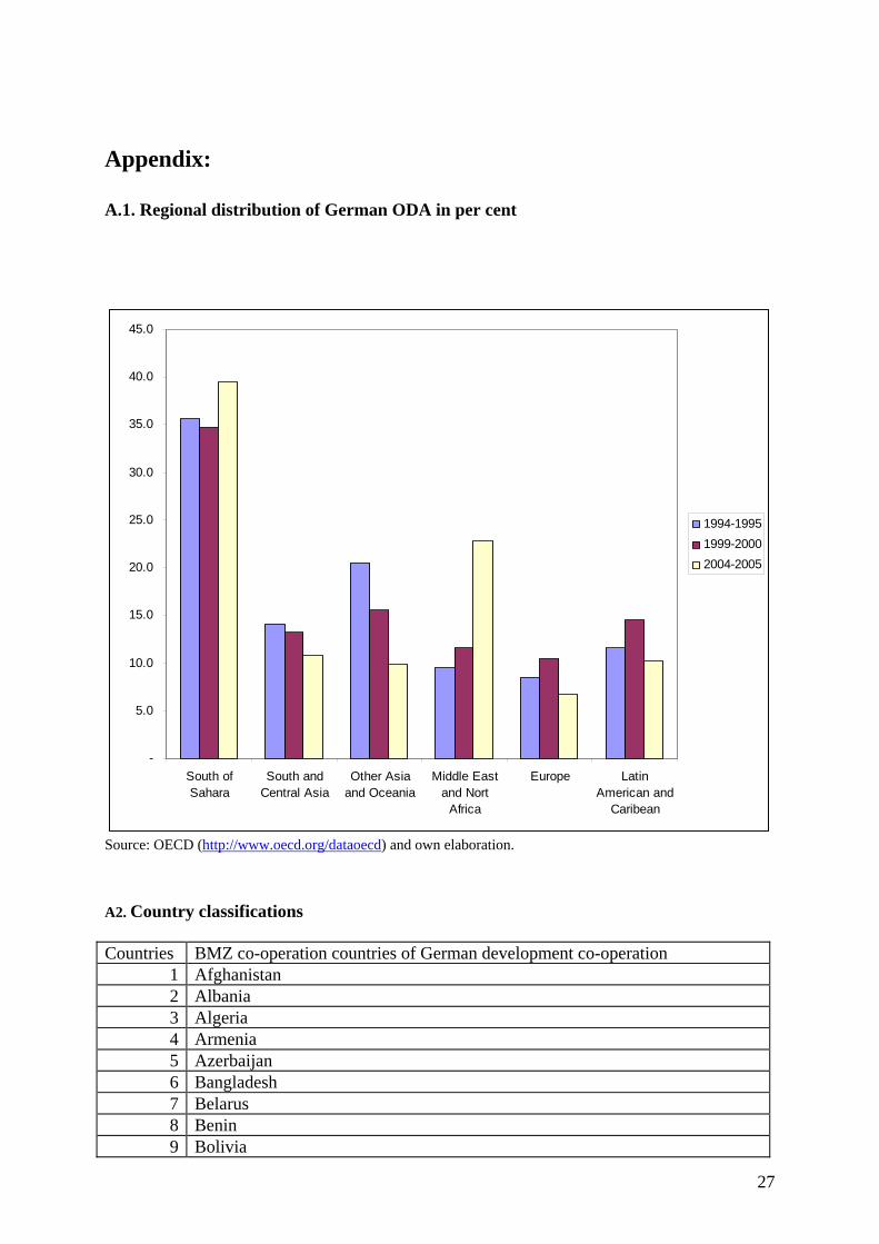
Appendix:

A.1. Regional distribution of German ODA in per cent

-

5.0

10.0

15.0

20.0

25.0

30.0

35.0

40.0

45.0

South ofSahara

South andCentral Asia

Other Asiaand Oceania

Middle Eastand Nort

Africa

Europe LatinAmerican and

Caribean

1994-19951999-20002004-2005

Source: OECD (http://www.oecd.org/dataoecd) and own elaboration.

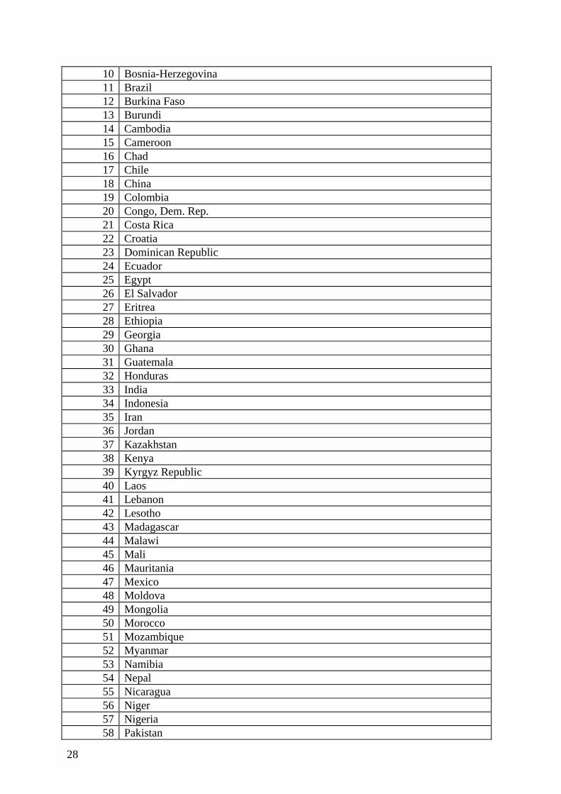
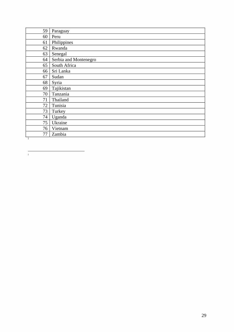
A2. Country classifications Countries BMZ co-operation countries of German development co-operation

1 Afghanistan 2 Albania 3 Algeria 4 Armenia 5 Azerbaijan 6 Bangladesh 7 Belarus 8 Benin 9 Bolivia

28

10 Bosnia-Herzegovina 11 Brazil 12 Burkina Faso 13 Burundi 14 Cambodia 15 Cameroon 16 Chad 17 Chile 18 China 19 Colombia 20 Congo, Dem. Rep. 21 Costa Rica 22 Croatia 23 Dominican Republic 24 Ecuador 25 Egypt 26 El Salvador 27 Eritrea 28 Ethiopia 29 Georgia 30 Ghana 31 Guatemala 32 Honduras 33 India 34 Indonesia 35 Iran 36 Jordan 37 Kazakhstan 38 Kenya 39 Kyrgyz Republic 40 Laos 41 Lebanon 42 Lesotho 43 Madagascar 44 Malawi 45 Mali 46 Mauritania 47 Mexico 48 Moldova 49 Mongolia 50 Morocco 51 Mozambique 52 Myanmar 53 Namibia 54 Nepal 55 Nicaragua 56 Niger 57 Nigeria 58 Pakistan

29

59 Paraguay 60 Peru 61 Philippines 62 Rwanda 63 Senegal 64 Serbia and Montenegro 65 South Africa 66 Sri Lanka 67 Sudan 68 Syria 69 Tajikistan 70 Tanzania 71 Thailand 72 Tunisia 73 Turkey 74 Uganda 75 Ukraine 76 Vietnam 77 Zambia

i

i