i. simple linear oscillators
TRANSCRIPT

I. Simple linear oscillators
A. Definitions and Background
Oscillators are a basic element in any measurement system and, in particular, are the core elementin any clocks. By definition, an oscillator is a device that produces a signal that varies sinusoidallyas a function of time, so that if s is the signal and t is time, we have s(t) = s0 cos(ωt +φ0), wheres0 and φ0 are constants, and ω = f/2π is the angular frequency and f is the usual frequency,measured in Hz or s−1. The signal can be a mechanical signal. Examples are the oscillations of apendulum or a tuning fork. Typical frequencies for a pendulum clock are on the order of 1 Hz, whiletypical frequencies for a tuning fork are on the order of 500 Hz. The signal can be an electricalsignal. Typical frequencies in this case range from a few kilohertz to hundreds of MHz. The signalscan come from crystal vibrations. Quartz crystal oscillators, which are the workhorse of mosttimekeeping systems, oscillate at frequencies from a few kHz to tens of MHz. The best oscillatorsuse atomic transitions. When an atom or molecule gives up energy, it emits a pure electromagneticwave. The oscillations in this case are at much higher frequencies. For cesium atoms, which arethe basis of modern-day atomic clocks, the frequency is close to 10×109 Hz or 10 GHz. Opticaltransitions occur at frequencies that are up to 100,000 times higher. Clocks are currently beingdeveloped at NIST that use a lattice of Yb atoms and that have an oscillation frequency of about500×1012 Hz or 500 THz.
Operation at higher frequency is important because clocks are made by counting the number ofzero crossings. A larger number of zero-crossings per second makes it possible to develop moreaccurate clocks.
Strictly speaking, an oscillator does not have to produce a sinusoidal signal. It is sufficient forthe signal to repeat periodically, so that s(t +T ) = s(t), and in fact real oscillators do not producestrictly sinusoidal signals. Some nonlinearity is always present. However, it is a remarkable fact ofnature that any oscillator, when it operates at a sufficiently low amplitude, will become sinusoidal.Moreover, any real oscillator will not operate with an absolutely constant amplitude s0 and phaseφ0. There are always noise sources that make these quantities fluctuate (vary around its averagevalue) or drift (walk away from its initial value). We will characterize these effects later.
B. Second-Order Linear Oscillators
The simplest model of a mechanical oscillator is a mass on a spring oscillating around a fixedequilibrium value x0 = 0, as shown in Fig. I.1.a. The force that the mass m experiences is given byF =−kx, where x is the distance away from the equilibrium value and k is the spring constant. Inthis case, Newton’s force law tells us that F = ma, where a is the acceleration or
md2xdt2 =−kx. (I.1)
Equation I.1 is a second-order linear differential equation with constant coefficients. It will beuseful in the future to rewrite this equation as two first-order equations. If we define the velocityv = dx/dt, we find that Eq. (I.1) becomes
dxdt
= v,dvdt
=− km
x. (I.2)
1
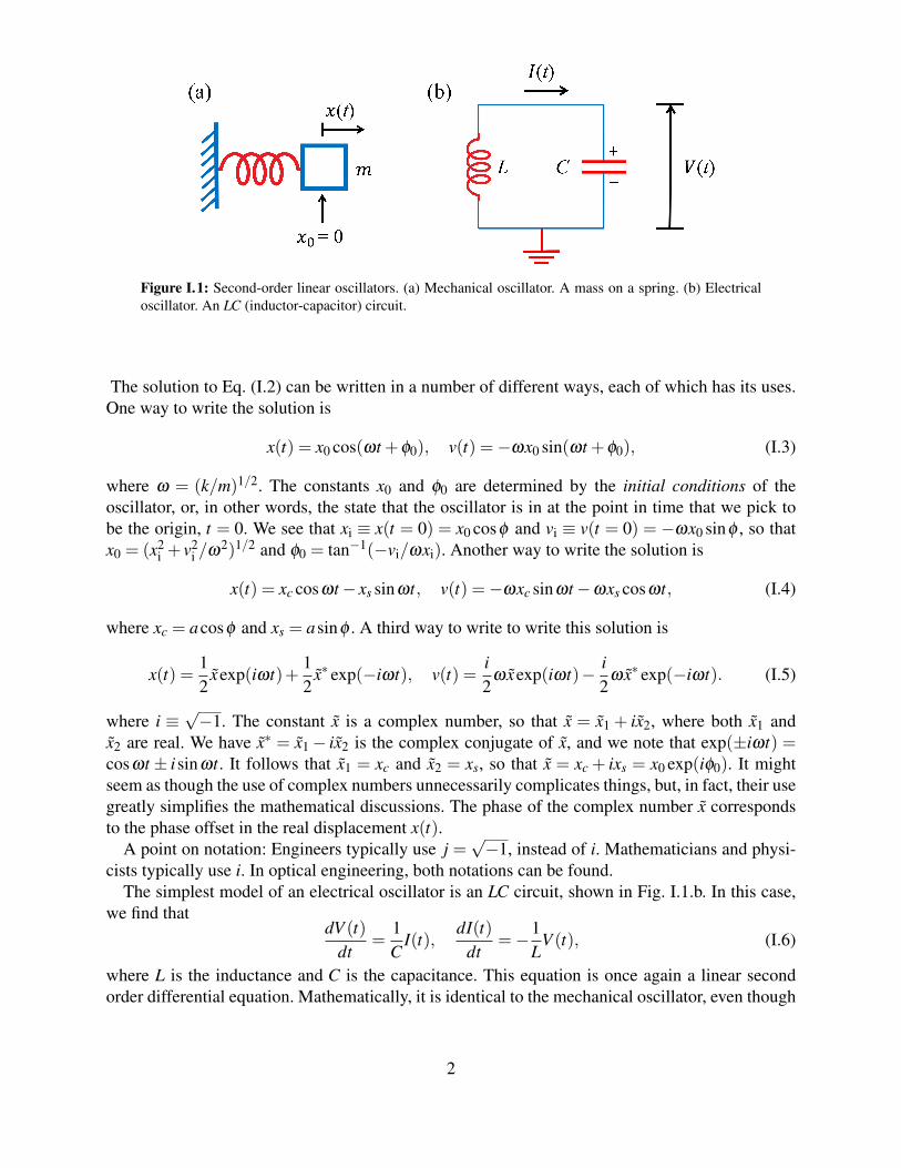
Figure I.1: Second-order linear oscillators. (a) Mechanical oscillator. A mass on a spring. (b) Electricaloscillator. An LC (inductor-capacitor) circuit.
The solution to Eq. (I.2) can be written in a number of different ways, each of which has its uses.One way to write the solution is
x(t) = x0 cos(ωt +φ0), v(t) =−ωx0 sin(ωt +φ0), (I.3)
where ω = (k/m)1/2. The constants x0 and φ0 are determined by the initial conditions of theoscillator, or, in other words, the state that the oscillator is in at the point in time that we pick tobe the origin, t = 0. We see that xi ≡ x(t = 0) = x0 cosφ and vi ≡ v(t = 0) = −ωx0 sinφ , so thatx0 = (x2
i + v2i /ω2)1/2 and φ0 = tan−1(−vi/ωxi). Another way to write the solution is
x(t) = xc cosωt− xs sinωt, v(t) =−ωxc sinωt−ωxs cosωt, (I.4)
where xc = acosφ and xs = asinφ . A third way to write to write this solution is
x(t) =12
xexp(iωt)+12
x∗ exp(−iωt), v(t) =i2
ω xexp(iωt)− i2
ω x∗ exp(−iωt). (I.5)
where i ≡√−1. The constant x is a complex number, so that x = x1 + ix2, where both x1 and
x2 are real. We have x∗ = x1− ix2 is the complex conjugate of x, and we note that exp(±iωt) =cosωt ± isinωt. It follows that x1 = xc and x2 = xs, so that x = xc + ixs = x0 exp(iφ0). It mightseem as though the use of complex numbers unnecessarily complicates things, but, in fact, their usegreatly simplifies the mathematical discussions. The phase of the complex number x correspondsto the phase offset in the real displacement x(t).
A point on notation: Engineers typically use j =√−1, instead of i. Mathematicians and physi-
cists typically use i. In optical engineering, both notations can be found.The simplest model of an electrical oscillator is an LC circuit, shown in Fig. I.1.b. In this case,
we find thatdV (t)
dt=
1C
I(t),dI(t)
dt=−1
LV (t), (I.6)
where L is the inductance and C is the capacitance. This equation is once again a linear secondorder differential equation. Mathematically, it is identical to the mechanical oscillator, even though
2

the physical system is completely different. Same equations; same solutions! So, we can just writedown the solution,
V (t) =12
V exp(iωt)+ c.c., I(t) =i
2Z0V exp(iωt)+ c.c, (I.7)
where c.c. is short for complex conjugate, ω = 1/(LC)1/2, Z0 = (L/C)1/2 is the characteristicimpedance of the circuit, and V = V1 + iV2 is determined by the initial conditions. We have V1 =V (t = 0) and V2 =−I(t = 0)Z0.
C. Visualizing the Solutions
In order to understand these solutions, it is useful to plot them. We will use MATLAB for thispurpose. MATLAB is a high-level programming language that has embedded in it many specialfunctions and routines that are necessary for engineering and physics. It also has numerous routinesfor plotting. UMBC has a license; so, it is available to all UMBC students for free.
When plotting solutions, it is necessary to pick a normalization for the quantities since comput-ers work with non-dimensional quantities. It is possible to normalize with respect to the standardSI (Systeme International) units. The SI units are the basic units in terms of which all other unitsare defined [s = second, kg = kilogram, m = meter, A = ampere, K = kelvin, mol = mole, cd =candela]. However, it is usually better to work in units that correspond to the physical system. Innormalizing time, we are typically interested in times that are short compared to a second; so, wemight use units of ms (milliseconds, 10−3 s), µs (microseconds, 10−6 s), ns (nanoseconds, 10−9 s),or ps (picoseconds, 10−12 s). In normalizing frequencies, we are typically interested in frequenciesthat are bigger than 1 Hz; so, we might use units of kHz (kilohertz, 103 Hz), MHz (megahertz,106 Hz), GHz (gigahertz, 109 Hz), or THz (terahertz, 1012 Hz).
In a typical laboratory experiment with a mass on a spring, the mass might equal 10 grams or10−2 kg in standard SI units. The spring might have a spring constant of 10 N/m. In this case,the radial frequency is given by ω = [10/10−2]1/2 = 31.3 s−1, so the usual frequency is givenby f = ω/2π = 5.03 Hz, which means that the weight will oscillate about five times per second.Hence, normalizing with respect to the second makes sense. A typical maximum length x0 mightbe on the order of 1 cm (10−2 m), so that normalizing lengths with respect to 1 cm makes sense.In this case, we find that the maximum velocity is given by ωx0 = 0.316 m/s.
If we consider a typical laboratory experiment with an LC circuit, the capacitor might have acapacitance of 100 pF (10−10 F = 10−10 s4A2kg−1m−2) and the inductor might have an inductanceof 1 mH (10−3 H = 10−3 s−2A−2kg m2). In this case, we find that ω = 3.16× 10⁶ s−1, so thatf = 503 kHz or f = 0.503 MHz. So, it makes sense to work in units of kHz or perhaps MHz. In10 µs, there are about five oscillations. If the amplitude of the voltage is 1 V, then the characteristicimpedance is given by Z0 = (10−3/10−10)1/2 ohms = 3.16×10³ Ω = 3.16 kΩ. The amplitude ofthe current is then given by I0 = 0.316 mA or 316 µA.
Figure I.2.a shows plots of the voltage and current as a function of time for five periods. Fig-ure I.2.b shows phase plots in which both the current and voltage are plotted as time varies. Phaseplots are useful as they show qualitative features of the evolution that time plots don’t reveal, andwe will use them many times. We see that the phase plots close in on themselves, which corre-sponds to the pattern repeating periodically, as is required for a good oscillator. Here, we showthree different cases, corresponding to V0 = 0.5, 0.7, and 0.9. The curves are elliptical in shape
3

Vol
tage
(V
)
time ( s)
Cur
rent
(m
A)
Current (mA)
Vol
tage
(V
)
Phase plot: Voltage vs. Current
(a)
(b)
Figure I.2: Plots of the voltage and current (a) as a function of time and (b) as phase plots.
because the oscillator energy is constant. The energy of the mechanical oscillator is given by
U =12
mv2 +12
kx2, (I.8)
and the energy of the electrical oscillator is given by
U =12
LI2 +1
2CV 2. (I.9)
4

Figure I.3: Parallel RLC circuit.
D. Damped-Driven Oscillators
In reality, all physical systems are damped. In the case of the mechanical oscillators, our equationsbecome
dxdt
= v,dvdt
=−αv− km
x, (I.10)
For the electrical oscillator, if we consider the RLC circuit that we show in Fig. I.3, we find
dVdt
=1C
I,dIdt
=− 1RC
I− 1L
V, (I.11)
where R is the resistance. Loss in this circuit is reduced when the resistance is large so that there islittle current flow through the resistor. Focusing on the electrical oscillator, we find that Eq. (I.11)has the general solution
V (t) =12
V+ exp(λ+t)+12
V− exp(λ−t), I(t) =λ+
2V+ exp(λ+t)+
λ−2
V− exp(λ−t), (I.12)
where
λ± =− 12RC±
[(1
2RC
)2
− 1LC
]1/2
. (I.13)
We see that if (1/2RC)2 > 1/LC, then both λ+ and λ− are real, while if 1/LC > (1/2RC)2, thenλ+ and λ− are complex conjugate numbers. For oscillators, we are interested in the second case,where the damping is small. In this case, we find λ+ = iω− γ , where
ω =
[1
LC−(
12RC
)2]1/2
=1
(LC)1/2
[1− 1
8L
R2C+ · · ·
]1/2
' 1(LC)1/2 , (I.14)
where we have written a Taylor expansion for ω , and we have just kept the lowest-order term. Wefind γ = 1/2RC. In this limit, we may write
V (t) =12
V exp[(iω− γ)t]+ c.c., I(t) =i
2ZV exp[(iω− γ)t]+ c.c., (I.15)
where 1/Z = (ω + iγ)C. Hence, the voltage and current are no longer exactly π/2 out of phase.Writing the voltage and current explicitly as real quantities, we find
5

Current (mA)
Vol
tage
(V
)
Phase plot: Voltage vs. Current
Current (mA)
Vol
tage
(V
)
Phase plot: Voltage vs. Current
(a)
(b)
Figure I.4: Phase plots of driven-damped oscillators. (a) The damped oscillator without driving. The phasetrajectory tends to zero. (b) The driven oscillator with a single driving frequency and two different initialconditions. The trajectory in both cases tends toward the driven solution, shown in blue.
V (t) =V0 cos(ωt +φ0)exp(−γ t),
I(t) =−V0
Z0sin(ωt +φ0 +φoff)exp(−γ t),
(I.16)
where V0 and φ0 are two constants determined by the initial conditions, and φoff = tan−1(γ/ω)Returning to the oscillator circuit that we considered in Sec. I.C and setting the resistance R
equal to 50 kΩ, V0 = 1 V, and φ0 = 0, we show the evolution in Fig. I.4.a. The resistance causesthe voltage and current to spiral into the origin, ultimately damping away completely.
6

Figure I.5: RLC circuit with a current source.
D.1. A single frequency driver
This “death spiral” is of course unacceptable in real oscillators, and it must be compensated bya source of energy that makes up for the loss. So, for example, in the RLC circuit that we areconsidering, we can add a current source, as shown in Fig. I.5. Writing the time derivative of thecurrent source J(t) as J′(t), we find that the equations that govern the voltage and current become
dVdt− 1
CI = 0,
dIdt
+1
RCI +
1L
V = J′. (I.17)
Equation (I.17) is referred to as an inhomegeneous linear equation because of the driving term, asopposed to Eqs. (I.1), (I.2), (I.6), (I.10), and (I.11), all of which are homogeneous linear equations.The term J′ is referred to as the inhomogeneous term.
We begin by considering the case where the driver is a pure oscillating signal, so that
J = J0 cos(ωt +φ0) =12
J exp(iωt)+ c.c., (I.18)
where J0 and φ0 are constants, and J = J0 exp(iφ0) is a complex constant. We will denote theresonant frequency of the oscillator as ω r = (1/LC)1/2. The driven solution is referred to as aparticular solution.
It is useful to choose the time origin so that φ0 = 0, in which case J = J0 is purely real. Becauseour equations are linear, we can find the solutions for V (t) and I(t) by just setting J(t)= J exp(iωt),so that J′ = iω J exp(iωt) and then taking the real part at the end. That turns out to be the simplestapproach mathematically. There will be an initial transient that damps out, after which both I(t)and V (t) will be proportional to exp(iωt). Writing I(t) = I exp(iωt) and V (t) = V exp(iωt), wefind
V =iωC
Jω2
r −ω2 +2iωγ=
iωC
ω2r −ω2−2iωγ
(ω2r −ω2)2 +4ω2γ2 J,
I =− ω2Jω2
r −ω2 +2iωγ=−ω2(ω2
r −ω2−2iωγ)
(ω2r −ω2)2 +4ω2γ2 J.
(I.19)
7

We then find that the real driven solutions, VD(t) and ID(t) are given by
VD(t) =ω
ω rZ0J0AD cos(ωt +φD) =
ω
ω rZ0J0AD [cosφD cosωt− sinφD sinωt]
=VDc cosωt−VDs sinωt,
ID(t) =−ω2
ω2r
J0AD sin(ωt +φD) =−ω2
ω2r
J0AD [sinφD cosωt + cosφD sinωt] ,
− ω
ω r
1Z0
(VDs cosωt +VDc sinωt) ,
(I.20)
AD =ω2
r
[(ω2r −ω2)2 +4ω2γ2]
1/2 ,
sinφD =ω2
r −ω2
[(ω2r −ω2)2 +4ω2γ2]
1/2 , cosφD =2ωγ
[(ω2r −ω2)2 +4ω2γ2]
1/2 ,
VDc = AD cosφD, VDs = AD sinφD.
(I.21)
We now rewrite the transient solution in Eq. (I.16) in the form
VT(t) =V0 cos(ωosct +φ0)exp(−γt) = [Vc cosωosct−Vs sinωosct]exp(−γt),
IT(t) =−ωosc
ω r
1Z0
[(Vc−
γ
ωoscVs
)sinωosct +
(Vs +
γ
ωoscVc
)cosωosct
]exp(−γ t),
(I.22)
where ωosc = (ω2r − γ2)1/2 is the natural frequency of the oscillator, Vc =V0 cosφ0, Vs =V0 sinφ0,
and we note that sinφoff = γ/ω r, cosφoff = ωosc/ω r. Rewriting Eq. (I.16), makes it easy to expressthe total current in terms of the initial conditions. The total voltage and current are given by V (t) =VD(t)+VT(t) and I(t) = ID(t)+ IT(t). Writing Vc and Vs in terms of the initial conditions, we find
Vc =V (t = 0)−VDc, Vs =−ω r
ωosc[Z0I(t = 0)−VDs]−
γ
ωoscVc. (I.23)
In Fig. I.4.b, we show the transient evolution of the the voltage V (t) vs. the current I(t) when thedriving current J0 = 10 µA, and we set ω = ω r. We show two cases. In both cases, the initialcurrent is 0; in the first case, the initial voltage is 0 V, and in the second case, the initial voltage is1 V. While in both cases, the transient evolution ultimately approaches the driven oscillation, theapproach is slow once the trajectory nears the final trajectory, shown in blue. This slow approachis not desirable in practice, and we will show later that it is possible to use nonlinearity to force afaster approach to the final oscillating state.
A point that may appear surprising at first is that the current oscillations are much larger than thedriving current. However, most of the current oscillates back and forth between the inductor andthe capacitor; a relatively small amount of drive current is needed to compensate for the loss in theresistor. The ratio of the ω r/γ in our illustration (' 30) is relatively small, and our oscillator is infact a poor oscillator! We chose this small value in order to be able to illustrate the damping andtransient effects. In fact, any useful oscillator will have ratios that are many orders of magnitudehigher. Some loss is however essential. In order to use the oscillator, we must be able to measure thevoltage, and that is done by having a load, which implies resistance and some loss. The same holdstrue for mechanical oscillators, where the displacement must be measured, or atomic oscillators,
8
where emission from a higher energy state to a lower energy state is accompanied by radiationand energy loss. In the case of our electrical oscillator, the energy dissipation Udiss during oneoscillation period, once the transient oscillations have ended, is given by
Udiss =∫ 2π/ω
0[V 2(t)/R]dt =
π
ωRZ2
0J20
ω2
ω2r
A2D. (I.24)
The rate at which energy transfers to the load on average is
dUdt
=1
2RZ2
0J20
ω2
ω2r
A2D. (I.25)
D.2. A broadband driver
In the solution that we just obtained, we assumed that the driver is itself a perfect oscillator withan ideal sinusoidal variation in time. However, the purpose of an oscillator is to take an imperfectdriver that has many different driving frequencies and turn it into a nearly pure signal. If we nowconsider a driver that consists of N different driving frequencies, we have
J(t) =N
∑n=1
Jn cos(ωnt +φn). (I.26)
If we have a broadband source, then we may assume that Jn = J0 is constant over the range offrequencies that can couple efficiently to the oscillator. We then find that
dUdt
=1
2RZ2
0J20
N
∑n=1
ω2
ω2r
A2D(ωn). (I.27)
In the limit of practical interest, in which ω r/γ 1, we can neglect the difference between ω andω r in Eq. (I.27), except for the term in the denominator in which (ω2
r −ω2) appears. Even thisterm can be rewritten as (ω2
r −ω2)' 2ω r(ω r−ω). We now find that
A2D(ω)' 1
4ω2
r(ω−ω r)2 + γ2 . (I.28)
We see that the A2D falls to half its maximum value when ∆ω ≡ ω−ω r = γ .
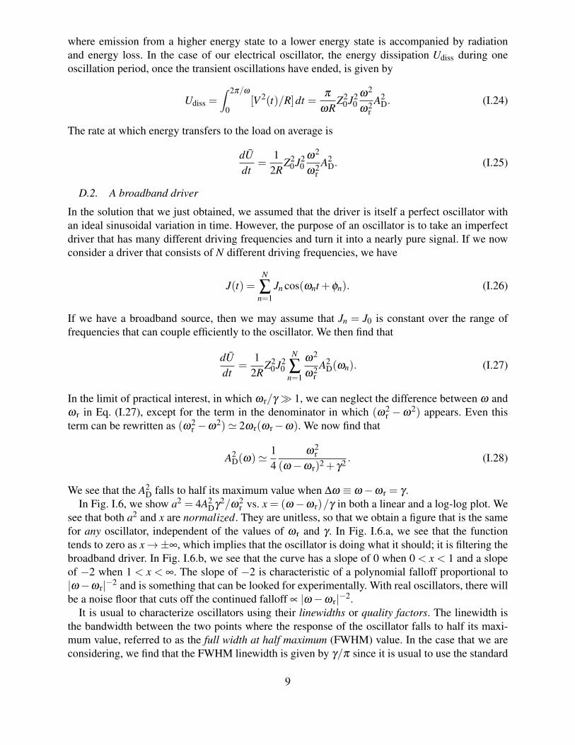
In Fig. I.6, we show a2 = 4A2Dγ2/ω2
r vs. x = (ω−ω r)/γ in both a linear and a log-log plot. Wesee that both a2 and x are normalized. They are unitless, so that we obtain a figure that is the samefor any oscillator, independent of the values of ω r and γ . In Fig. I.6.a, we see that the functiontends to zero as x→±∞, which implies that the oscillator is doing what it should; it is filtering thebroadband driver. In Fig. I.6.b, we see that the curve has a slope of 0 when 0 < x < 1 and a slopeof −2 when 1 < x < ∞. The slope of −2 is characteristic of a polynomial falloff proportional to|ω−ω r|−2 and is something that can be looked for experimentally. With real oscillators, there willbe a noise floor that cuts off the continued falloff ∝ |ω−ω r|−2.
It is usual to characterize oscillators using their linewidths or quality factors. The linewidth isthe bandwidth between the two points where the response of the oscillator falls to half its maxi-mum value, referred to as the full width at half maximum (FWHM) value. In the case that we areconsidering, we find that the FWHM linewidth is given by γ/π since it is usual to use the standard
9

(a)
(b)
Figure I.6: (a) Linear and (b) log-log plots of 4A2Dγ2/ω2
r vs. (ω−ω r)/γ . In (a) we illustrate the FWHMwidth in the angular frequency. In (b) we show the characteristic slopes of 4A2
Dγ2/ω2r when 0≤ x < 1 and
−2 when x > 1 in a log-log plot.
frequency, rather than the angular frequency when quoting linewidths. The quality factor (Q) is de-
10

fined in two different ways that are not exactly equivalent. The first is Q = f/∆ f , where ∆ f is theFWHM linewidth and f is the resonant frequency. For the linear oscillator, we find that Q=ω r/2γ .Another way to define Q is
Q = 2π× energy storedenergy dissipated per cycle
. (I.29)
For the electrical oscillator that we considered, the energy stored is given by Ustored = (L/2)I2max =
(1/2C)V 2max, where Imax is the maximum current flowing through the inductor, Vmax is the maxi-
mum voltage at the capacitor, and we note that the stored energy oscillates back and forth betweenthe two. From Eq. (I.20), we see that (L/2)I2
max = (L/2)J20 A2
D. From Eq. (I.24), we see that in thelimit of interest to us (ω 'ω r), Udiss = (2π/ω r)(L/2RC)J2
0 A2D. Recalling that γ = 1/2RC, we find
that Q = 2π(Ustored/Udiss) = 2γ/ω r, which is the same result that we obtained with our previousdefinition. These two definitions are equivalent for any linear oscillator with a single oscillationfrequency, regardless of whether the oscillator is electrical or mechanical.
E. Matrix Representations: Eigenvalues and Eigenvectors
To find the oscillation frequencies in Eq. (I.3), (I.7), and (I.14), we can use a simple algebraicapproach. To find V and I in Eq. (I.19), we can also use a simple algebraic approach in which wefirst eliminate one of the variables, solve for the second, and substitute to find the first. However,this ad hoc approach no longer works well when we consider more complex system. Instead, it isbetter to use the methods of linear algebra in which we use matrix representations.
We begin by defining a 2×1 column vector
u =
[u1u2
], (I.30)
where u1 = x and u2 = v for the mechanical oscillator, and u1 = V and u2 = I for the electricaloscillator. We can now write the equations that govern the oscillator as
dudt
= Au, (I.31)
where
A=
[A11 A12A21 A22
](I.32)
is a 2×2 matrix. The rule for multiplying a 2×2 matrix and 2×1 column vector is
v = Au↔ vm =2
∑n=1
Amnun, (I.33)
where v is also a 2× 1 column vector. For the mechanical driven-damped oscillator, we haveA11 = 0, A12 = 1, A21 = −k/m, and A22 = −α . For the electrical oscillator, we have A11 = 0,A12 = 1/C, A21 =−1/L, A22 =−1/RC.
To find the oscillation frequencies, we search for solutions that have the form du/dt = λu sincewe know that the solution of (almost) any linear ordinary differential equation is composed ofthe sum of functions that vary exponentially in time. (The small caveat is that in some cases,
11

Figure I.7: Schematic illustration of (a) non-independent and (b) independent eigenvalue equations. Whenthe equations are not independent, they define lines that lie on top of each other, shown as a red-blue dashedline. When the equations are independent, they define lines that only meet at u1 = u2 = 0.
the exponentials have to multiplied by polynomials in time.) Writing u = uexp(λ t), Eq. (I.31)becomes
λ u = Au or (A−λ I)u = 0, (I.34)
where I is the identity matrix, whose elements are given by I11 = 1, I12 = 0, I21 = 0, and I22 = 1.This equation is an eigenvalue equation. Eigenvalue equations play an important role in almostevery area of science and engineering; so, there are many textbooks that describe their properties,as well as computational implementations that solve these equations. We will take advantage ofthe MATLAB implementations. We see that one solution to Eq. (I.34) is the trivial solution u = 0.In order for there to be non-trivial solutions, the two equations that make up the matrix equation(A11−λ )u1 +A12u2 = 0 and A12u1 +(A22−λ )u2 = 0 must be effectively the same equation. Ifwe plot u2 vs. u1, we see that both equations correspond to lines that pass through zero. Eitherthe slopes on the same, in which case they corresponds to the same line, as shown in Fig. I.7.a,or the slopes are different, shown in Fig. I.7.b, in which case the only solution is u1 = u2 = 0.In the former case, we say that the equations are not independent. More generally, we can alsosay that the determinant of the matrix A− λ I = 0, which is written det(A− λ I) = 0. For largedimensional systems, the eigenvalues and the oscillating frequencies are still determined by thecondition det(A−λ I) = 0. We will give a general definition of the determinant later. The deter-minant of any 2× 2 matrix B is given by B11B22−B12B21 and for our eigenvalue equation thatimplies (A11−λ )(A22−λ )−A12A21 = 0 or λ 2−λ (A11 +A22)+(A11A22−A12A21) = 0. We thusobtain a quadratic equation for λ . Substituting in the expressions for either the mechanical or elec-trical oscillator, we can obtain the same expressions for the complex oscillation frequencies thatwe obtained before. More generally, these values of λ are referred to as eigenvalues
Once we have found the eigenvalues, we can find corresponding values of u that solve theseequations. These are referred to as eigenvectors. For each eigenvalue, we can use either of thetwo rows of the eigenvalue equation. If we consider for example the electrical oscillator withoutdamping, we find that eigenvectors are given by
e+ =
[1
i/Z0
], e− =
[1
−i/Z0
], (I.35)
corresponding respectively to the eigenvalues λ+ = iω r and λ− = −iω r. Since the equations arelinear, any eigenvector when multiplied by a constant is also an eigenvector. These correspond
12

to all the points on the line that we show schematically in Fig. I.8.a. So, the general solution ofEq. (I.31) becomes
u =12
u+e+ exp(iω rt)+12
u−e− exp(−iω rt), (I.36)
where u+ and u− are complex constants that depend on the initial conditions. At t = 0, we see that
u(t = 0) =[V (t = 0)I(t = 0)
]=
[(1/2)(u++ u−)(i/2Z0)(u+− u−)
], (I.37)
from which we conclude u+ = V (t = 0)− iZ0I(t = 0) and u− = V (t = 0)+ iZ0I(t = 0). We seethat u+ and u− are complex conjugates, which ensures u is real at all times. Comparing Eq. (I.37)to Eq. (I.7), we see that V = u+. This solution is consistent with our earlier results. So, we havelearned nothing new. However, this approach is the best approach to use when considering higher-dimensional oscillators.
To solve the driven-damped oscillator equations use matrix methods, we first rewrite Eq. (I.17)in the form
dudt−Au = D, (I.38)
where
A=
[0 1/C−1/L 1/RC
], D =
[0J′
]. (I.39)
We assume that our driver D is at a single frequency, so that D = Dexp(iωt), where D is a knownconstant vector, and we search for solutions in the form u = uexp(iωt), where u is an unknownconstant vector. Writing out these vectors, we have
D =
[0
iω J
]and u =
[VI
]. (I.40)
Equation (I.38) now becomesBu = D, (I.41)
where B= iω I−A. To solve Eq. (I.41), we may use the inverse of B, written as B−1. This matrixsatisfies the relation B−1B= BB−1 = I. It then follows that
u = B−1D. (I.42)
In general, it is not efficient to solve matrix equations using the inverse when the system of equa-tions becomes large. It is better to use Gauss-Jordan elimination. However, this approach workswell for the second-order system that we are considering here. The inverse of a matrix B is givenby
B−1 =1
det(B)
[B22 −B12−B12 B11
], (I.43)
which becomes explicitly in this case
B−1 =1
[iω (iω−1/RC)+1/LC]
[iω +1/RC 1/C−1/L iω
]. (I.44)
Operating with B−1 on D and using the relations 1/RC = 2γ , 1/LC = ω2r , we obtain Eq. (I.19).
13
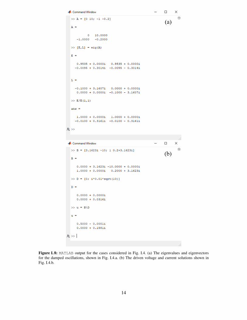
Figure I. 8: MATLAB output for the cases considered in Fig. I.4. (a) The eigenvalues and eigenvectorsfor the damped oscillations, shown in Fig. I.4.a. (b) The driven voltage and current solutions shown inFig. I.4.b.
14

Due to the importance of linear algebra in a wide variety of applications, MATLAB has imple-mented a powerful set of algorithms to solve eigenvalue problems and linear systems of equations.For the numerical examples that we presented in Fig. I.4, we have C = 10−10, L = 10−3, andR = 5×10⁴ in appropriate SI units. Explicitly, we then have
A=
[0 1010
−103 −2×10⁵ω
]. (I.45)
In general, it is not good computational practice to use numbers with large exponents. It is better touse quantities that are all on the order of one by appropriately renormalizing quantities. If we usemicroseconds instead of seconds and we use milliamperes instead of amperes, our matrix becomes
A=
[0 10−1−0.2
]. (I.46)
and we see that none of the quantities differs too much from one. This sort of dimensional analysisalso gives us an immediate feel for the rough value that quantities will have. Frequencies will be onthe order a megahertz, voltages will be on the order of one volt, and currents will be on the orderof milliamperes. That is consistent with the results that we already plotted in Fig. I.2.
To find the eigenvalues and eigenvectors, we may use MATLAB’s eig routine. The command[E,L] = eig(A) produces the eigenvalues λ± = −0.1± 3.1607i, which are the diagonal ele-ments of the matrix L. We show the output in Fig. I.6.a. This command also produces the eigen-vectors e± = [0.9535,−.0095±0.3014]t , where t denotes the transpose, so that
[0.9535,−.0095±0.3014]t =[
0.9535−.0095±0.3014
].
The eigenvectors appear as the columns of the matrix E = [e+,e−]. MATLAB uses the l2 norm foreigenvectors in which the sum of the absolute squares equals 1. In order to put the eigenvectors inthe form where the first element of e+ and e− both equal 1.0, we divide E by E11, which yieldse± = [1.0,−0.01± 0.3161i]. We infer that γ = 0.1 µs−1 and ωosc = 3.1607 µs−1, correspondingto an oscillation frequency of 0.503 MHz or 503 kHz, which is what we found earlier. We infer aswell that i/Z = (i/Z0)(ωosc/ω r + iγ/ω r) = −0.01+ 0.3161i kΩ−1, so that Z0 = |Z| = 3.162 kΩ,which is again consistent with our earlier result.
To find u = [V , I]t for the case driven solution that we considered in Fig. I.4, we first recallthat ω = ω r =
√10 = 3.1623 µs−1 in the case that we considered. We also recall that iω J =
i√
10×0.01 mA-µs−1. Hence, we find
B=
[i√
10 −101 i√
10+0.2
], D =
[0
i0.01√
10
]. (I.47)
To find u = [V , I]t , we use the MATLAB command u = B\D. This command uses Gauss-Jordanelimination to solve for u. We show the results in Fig. I.6.b. We find V = 0.5 V and I = 0.1581i mA,which equals 158 µA. These results are consistent with our prior results.
ExercisesThese exercises combine investigative exercises that require you to do some on-line research (I),
mathematical or computational exercises that require you to verify the steps in the calculations ofthis section or extend them (M), and experimental exercises that require you to build something totest the ideas in this section (E).
15

1. (I) The most commonly used oscillators are quartz crystal oscillators. What is their operatingprinciple? What is its operating frequency range? What are typical quality factors?
2. (I) Rubidium and sapphire crystal oscillators are alternatives to quartz crystal oscillators.What are their advantages and disadvantages?
3. (I) The best oscillators are based on atomic transitions. Cesium transitions are the basis ofmodern-day atomic clocks. There is increasing interest in using transitions of an ytterbiumlattice, and future clocks are likely to based on these transitions. What are the operatingfrequencies and linewidths of these oscillators? What are the corresponding quality factors?
4. (M) For the mechanical oscillator that is described in Sec. I.C, modify the codeOscillatorI2 (part b) to make a phase plot of x vs. v for five cases where the maxi-mum excursion ranges between 1 cm and 4 cm. Calculate the energy that is stored in theoscillator for each of these cases.
5. (M) Verify Eq. (I.5) by substitution into the governing equation, Eq. (1.2), and relate x and vto the initial conditions.
6. (I and M) If we consider hydrogen-iodide (HI), which is a diatomic molecule, the hydrogenatom will vibrate in the potential well of the iodine atom. While a real understanding of themolecule must use quantum mechanics, a basic understanding can be obtained by treatingthe hydrogen atom as a simple second-order oscillator. The frequency of vibration can becalculated from the wavenumber of the emissions, which is 2230 cm−1 and the approximatemagnitude of the oscillations can be calculated from the dimension of the molecule, which is161 pm. The mass of the hydrogen atom is close to 1 atomic unit. Calculate the frequency ofvibration of the hydrogen atom and its mass in SI units. Use that information to calculate theeffective spring constant. Suppose that the energy stored in the vibrational motion is given byh f , where h is Planck’s constant and f is the oscillation frequency, how large an excursionis the hydrogen atom making and how does that compare to the size of the molecule?
7. (M) Derive Eq. (I.11) using Kirchhoff’s current law for the circuit of Fig. I.3.
8. (M) Verify Eqs. (I.12–I.16) by substitution into the governing equation, Eq. (I.11).
9. (M) Derive equivalent expressions to Eqs. (I.12-I.16) for the mechanical oscillator, describedby Eq. (1.10). For the example parameters of Sec. I.C, what damping rate α would corre-spond to γ/ω r = 1/100, 1/10
√10, and 1/10? Modify OscillatorI4 (part a) to make
phase plots for each of these cases.
10. (M) Verify Eqs. (1.19–1.23) by substitution into the governing equation, Eq. (I.17).
11. (M) Modify OscillatorI4 (part b) to plot the driven oscillation for five driving frequen-cies, equal to 0.25ω r, 0.5ω r, 1.0ω r, 1.5ω r, and 2.0ω r.
12. (M) Derive an expression for a mechanical oscillator that is equivalent to Eq. (I.17). Whatcorresponds physically to the driving current? Draw a corresponding picture.
16

13. (M) The expression for A2D that we derived, given in Eq. (I.28), is proportional to the
Lorentzian function,
fL(ω) =1π
γ
(ω−ω r)2 + γ2 .
(a) Show that∫
∞
−∞fL(ω)dω = 1.
(b) Use MATLAB to plot L(ω) vs. ω−ω r, assuming that γω r = 1/100, 1/10√
10, and 1/10.
(c) We stated that the expression for AD in Eq. (I.28) is a good approximation to the ex-act expression for AD in Eq. (I.21). Compare these expressions by plotting a(ω) =(2γ/ω r)AD(ω) vs. x = (ω −ω r)/γ for both these expressions and for γ/ω r = 1/2,1/10, and 1/100 on both linear and log-log plots, as in oscillatorI7. What are the slopesin the log-log plots for 0 < x < 1 and 1 < x < ∞?
14. (M) For our example mechanical oscillator, with the value of α given by γ/ω r = 1/10, findthe matrix A that corresponds to Eq. (I.39). Find the eigenvalues and eigenfunctions of thismatrix using MATLAB. Show the MATLAB ouput. Assume you have a driving force with anamplitude of 1 mN at the resonant frequency, find the matrix B, and use MATLAB to findu = [x, v]t . Show the MATLAB output. Write the real expressions x and v and use a modifiedversion of OscillatorI4 to draw a phase plot of the oscillation. How much energy isstored in the oscillator?
15. (M and I) MATLAB can work with symbols as well as numbers. Use this capability to obtainEq. (I.24) and a symbolic expression for u. Compare to Eq. (I.19).
16. (E) Obtain a kit for a mechanical oscillator with springs and weights. Measure the oscilla-tions as a function of time and compare to what is theoretically expected.
17. (E) Obtain a kit that will enable you to build an RLC oscillator. Measure the oscillations as afunction of time and compare to what is experimentally expected.
17
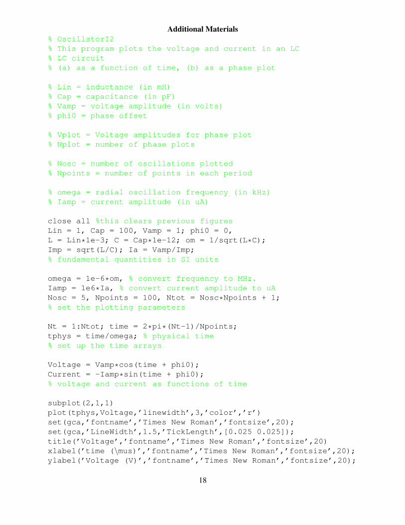
Additional Materials% OscillatorI2% This program plots the voltage and current in an LC% LC circuit% (a) as a function of time, (b) as a phase plot
% Lin = inductance (in mH)% Cap = capacitance (in pF)% Vamp = voltage amplitude (in volts)% phi0 = phase offset
% Vplot = Voltage amplitudes for phase plot% Nplot = number of phase plots
% Nosc = number of oscillations plotted% Npoints = number of points in each period
% omega = radial oscillation frequency (in kHz)% Iamp = current amplitude (in uA)
close all %this clears previous figuresLin = 1, Cap = 100, Vamp = 1; phi0 = 0,L = Lin*1e-3; C = Cap*1e-12; om = 1/sqrt(L*C);Imp = sqrt(L/C); Ia = Vamp/Imp;% fundamental quantities in SI units
omega = 1e-6*om, % convert frequency to MHz.Iamp = 1e6*Ia, % convert current amplitude to uANosc = 5, Npoints = 100, Ntot = Nosc*Npoints + 1;% set the plotting parameters
Nt = 1:Ntot; time = 2*pi*(Nt-1)/Npoints;tphys = time/omega; % physical time% set up the time arrays
Voltage = Vamp*cos(time + phi0);Current = -Iamp*sin(time + phi0);% voltage and current as functions of time
subplot(2,1,1)plot(tphys,Voltage,’linewidth’,3,’color’,’r’)set(gca,’fontname’,’Times New Roman’,’fontsize’,20);set(gca,’LineWidth’,1.5,’TickLength’,[0.025 0.025]);title(’Voltage’,’fontname’,’Times New Roman’,’fontsize’,20)xlabel(’time (\mus)’,’fontname’,’Times New Roman’,’fontsize’,20);ylabel(’Voltage (V)’,’fontname’,’Times New Roman’,’fontsize’,20);
18

axis tight;xlim([0 10])ylim([-1 1])set(gcf, ’WindowStyle’, ’normal’);set(gca, ’Unit’, ’inches’);set(gca, ’TickLabelInterpreter’,’LaTeX’,...’YTick’,[-1:1:1],’YTickLabel’,’$-1$’,’$0$’,’$1$’)set(gcf, ’PaperPosition’,1.9*[0 0 4 3],’PaperSize’,1.9*[4 3])
subplot(2,1,2)plot(tphys,.001*Current,’linewidth’,3,’color’,’r’)set(gca,’fontname’,’Times New Roman’,’fontsize’,20);set(gca,’LineWidth’,1.5,’TickLength’,[0.025 0.025]);title(’Current’,’fontname’,’Times New Roman’,’fontsize’,20)xlabel(’time (\mus)’,’fontname’,’Times New Roman’,’fontsize’,20);ylabel(’Current (mA)’,’fontname’,’Times New Roman’,’fontsize’,20);axis tight;xlim([0 10])ylim([-.500 .500])set(gcf, ’WindowStyle’, ’normal’);set(gca, ’Unit’, ’inches’);set(gca, ’TickLabelInterpreter’,’LaTeX’,...’YTick’,[-.500:.500:.500],’YTickLabel’,’$-0.5$’,’$0$’,’$0.5$’)set(gcf, ’PaperPosition’,1.9*[0 0 4 3],’PaperSize’,1.9*[4 3])saveas(gcf,’1.pdf’,’pdf’)
Vplot=[0.5 0.7 0.9], Nplot=3,% Set the values for the phase plots%figure%axis squareclose allfor Np=1:NplotVpl=Vplot(Np)*Voltage(1:Ntot);Ipl=.001*Vplot(Np)*Current(1:Ntot);plot(Ipl,Vpl,’linewidth’,3)hold on
endhold offannotation(’arrow’,’Position’,[0.739,0.5,0,0.005])% text(150.0,0.8,’V 0=0.9’,’fontname’,’Times NewRoman’,’fontsize’,16)annotation(’arrow’,’Position’,[0.689,0.5,0,0.005])% text(85.0,0.7,’V 0=0.7’,’fontname’,’Times NewRoman’,’fontsize’,16)annotation(’arrow’,’Position’,[0.640,0.5,0,0.005])
19

% text(10.0,0.55,’V 0=0.5’,’fontname’,’Times NewRoman’,’fontsize’,16)set(gca,’fontname’,’Times New Roman’,’fontsize’,20);set(gca,’LineWidth’,1.5,’TickLength’,[0.025 0.025]);title(’Phase plot: Voltage vs. Current’,’fontname’,’Times NewRoman’,’fontsize’,20)xlabel(’Current (mA)’,’fontname’,’Times New Roman’,’fontsize’,20)ylabel (’Voltage (V)’,’fontname’,’Times New Roman’,’fontsize’,20)xlim([-.500 .500]) %define limits for x axisylim([-1 1]) %define limits for y axisset(gcf, ’WindowStyle’, ’normal’);set(gca, ’Unit’, ’inches’);set(gca, ’TickLabelInterpreter’,’LaTeX’,...’YTick’,[-1:.5:1],’YTickLabel’,’$-1$’,’$-0.5$’,’$0$’,’$0.5$’,’$1$’)
set(gca, ’TickLabelInterpreter’,’LaTeX’,...’XTick’,[-.5:.25:.5],’XTickLabel’,’$-0.5$’,’$-0.25$’,’$0$’,’$0.25$’,’$0.5$’) %define the ticks and use LaTeX interpreter to have realminus signsset(gcf, ’PaperPosition’,1.9*[0 0 4 3],’PaperSize’,1.9*[4 3])%define the paper size and positionlgd = legend(’$V 0=0.5$ V’,’$V 0=0.7$ V’,’$V 0=0.9$ V’);%add the legend% legend(’Location’,’northwest’)set(lgd,’interpreter’,’latex’,’FontSize’,17);% set(lgd,’interpreter’,’latex’);legend (’boxoff’); %turn the box around the elegend offsaveas(gcf,’2.pdf’,’pdf’) %save file as a .pdf file
20

% OscillatorI4% This routine calculates phase diagrams for the parallel% RLC circuit% (a) without a driving voltage, (b) with a driving voltage
% Lin = inductance (in mH)% Cap = capacitance (in pF)% Res = resistance (in kOhms)
% V0a = initial voltage amplitude, part (a) (in volts)% I0a = initial current amplitude, part (a) (in uA)
% FreqRat = ratio of driving to resonant frequency,% part (b)% V0b = initial voltage amplitudes, part (b) (in volts)% J0 = driving current amplitude, part (b) (in uA)
% Nosc = number of oscillations plotted% Npoints = number of points in each period
% omega = natural oscillation frequency% gamma = damping rate% Imp = real impedance% phoff = phase offset
% omr = resonant frequency% gamRat = ratio of the damping and resonant frequencies% omRat = ratio of the resonant and natural frequencies% ADc = driving voltage amplitude;% CDc = cosine (driving angle)% SDc = sine (driving angle)% VDc, VDs = in-phase and quadrature quadratures of% the driving voltages
% [Current,Voltage] = current and voltage, part (a)
% Part (b):% [CurD,VolD] = driven current and voltage% [CurT1,VolT1] = transient current and voltage 1% [CurT2,VolT2] = transient current and voltage 2
close all
Lin = 1, Cap = 100, Res = 50, V0a = 1,FreqRat = 1.0, V0b = [0 1], J0 = 10,% set initial values
21

L = Lin*1e-3; C = Cap*1e-12; R = Res*1e3;% convert to SI unitsgamma = 1/(2*R*C); omega=((1/(L*C)) - gammaˆ2)ˆ(1/2);% compute the damping coefficient and frequencygam = gamma/omega; %compute the damping ratioImp = sqrt(L/C); phoff = atan(gamma/omega);% calculate the impedance amplitude and phase offsetIa = V0a/Imp; I0a = 1e6*Ia;% compute the initial current amplitude (part a) in uA
Jb = J0*1e-6 %convert to SI unitsomr = 1/sqrt(L*C); gamRat = gamma/omr;omRat = omr/omega;% compute the resonant frequency, damping ratio,% and resonant to natural frequency ratio% (part b)ADc = 1/((1-FreqRatˆ2)ˆ2 + 4*FreqRatˆ2*gamRatˆ2)ˆ(1/2);CDc = 2*FreqRat*gamRat*ADc; SDc = (1-FreqRatˆ2)*ADc;VDc = FreqRat*Imp*Jb*ADc*CDc;VDs = FreqRat*Imp*Jb*ADc*SDc;% in-phase and quadrature components of the driven% voltageVc1 = V0b(1) - VDc; Vc2 = V0b(2) - VDc;Vs1 = omRat*VDs - gam*Vc1;Vs2 = omRat*VDs - gam*Vc2;% transient voltage and current amplitude coefficients
Nosc = 15, Npoints = 100, Ntot = Nosc*Npoints + 1;% set the plotting parameters
Nt = 1:Ntot; time = 2*pi*(Nt-1)/Npoints;% set up the time array
% Part (a): Compute and plot voltage and currentVoltage = V0a*cos(time).*exp(-gam*time);Current = -I0a*sin(time + phoff).*exp(-gam*time);% voltage and current as functions of time
plot(.001*Current,Voltage,’linewidth’,1,’color’,’r’)% axis([-300,300,-1.0,1.0])% title(’Phase plot: Voltage vs. Current’)% xlabel(’Current (\muA)’)% ylabel (’Voltage (V)’)annotation(’arrow’,’Position’,[0.691,0.5,0,0.005])set(gca,’fontname’,’Times New Roman’,’fontsize’,20);
22

set(gca,’LineWidth’,1.5,’TickLength’,[0.025 0.025]);title(’Phase plot: Voltage vs. Current’,’fontname’,’Times NewRoman’,’fontsize’,20)xlabel(’Current (mA)’,’fontname’,’Times New Roman’,’fontsize’,20)ylabel (’Voltage (V)’,’fontname’,’Times New Roman’,’fontsize’,20)xlim([-.500 .500]) %define limits for x axisylim([-1 1]) %define limits for y axisset(gcf, ’WindowStyle’, ’normal’);set(gca, ’Unit’, ’inches’);set(gca, ’TickLabelInterpreter’,’LaTeX’,...’YTick’,[-1:.5:1],’YTickLabel’,’$-1$’,’$-0.5$’,’$0$’,’$0.5$’,’$1$’)
set(gca, ’TickLabelInterpreter’,’LaTeX’,...’XTick’,[-.5:.25:.5],’XTickLabel’,’$-0.5$’,’$-0.25$’,’$0$’,’$0.25$’,’$0.5$’) %define the ticks and use LaTeX interpreter to have realminus signsset(gcf, ’PaperPosition’,1.9*[0 0 4 3],’PaperSize’,1.9*[4 3])%define the paper size and positionsaveas(gcf,’3.pdf’,’pdf’) %save file as a .pdf file
% Part (b): Compute and plot the voltage and current% evolution, starting from the given initial conditions.% The initial current is assumed to equal zero.
FreqD = FreqRat*omRat; % driving frequencyVolD = VDc*cos(FreqD*time) - VDs*sin(FreqD*time);CurD = -(1/(omRat*Imp))*(VDs*cos(FreqD*time)...+ VDc*sin(FreqD*time)); CurD = CurD*1e6VolT1 = (Vc1*cos(time) - Vs1*sin(time)).*exp(-gam*time);CurT1 = -(1/(omRat*Imp))*((Vc1-gamRat*Vs1)*sin(time)...+(Vs1+gamRat*Vc1)*cos(time)).*exp(-gam*time);CurT1 = CurT1*1e6VolT2 = (Vc2*cos(time) - Vs2*sin(time)).*exp(-gam*time);CurT2 = -(1/(omRat*Imp))*((Vc2-gamRat*Vs2)*sin(time)...+(Vs2+gamRat*Vc2)*cos(time)).*exp(-gam*time);CurT2 = CurT2*1e6VolT1 = VolT1 + VolD; CurT1 = CurT1 + CurD;VolT2 = VolT2 + VolD; CurT2 = CurT2 + CurD;close allplot(.001*CurD,VolD,’LineWidth’,4)hold onplot(.001*CurT1,VolT1,’k’,.001*CurT2,VolT2)set(gca,’fontname’,’Times New Roman’,’fontsize’,20);set(gca,’LineWidth’,1.5,’TickLength’,[0.025 0.025]);title(’Phase plot: Voltage vs. Current’,’fontname’,’Times New
23

Roman’,’fontsize’,20)xlabel(’Current (mA)’,’fontname’,’Times New Roman’,’fontsize’,20)ylabel (’Voltage (V)’,’fontname’,’Times New Roman’,’fontsize’,20)xlim([-.500 .500]) %define limits for x axisylim([-1 1]) %define limits for y axisset(gcf, ’WindowStyle’, ’normal’);set(gca, ’Unit’, ’inches’);set(gca, ’TickLabelInterpreter’,’LaTeX’,...’YTick’,[-1:.5:1],’YTickLabel’,’$-1$’,’$-0.5$’,’$0$’,’$0.5$’,’$1$’)
set(gca, ’TickLabelInterpreter’,’LaTeX’,...’XTick’,[-.5:.25:.5],’XTickLabel’,’$-0.5$’,’$-0.25$’,’$0$’,’$0.25$’,’$0.5$’) %define the ticks and use LaTeX interpreter to have realminus signsset(gcf, ’PaperPosition’,1.9*[0 0 4 3],’PaperSize’,1.9*[4 3])%define the paper size and positionsaveas(gcf,’4.pdf’,’pdf’) %save file as a .pdf file
24

% OscillatorI6% This program plots the FWHM of the Lorentz(ian) function as% well as the Lorentz(ian) function for positive values in X in aloglog plot.% Where A Dˆ2 is the Eq. I.28 in the text% Y = 4*A Dˆ2*gammaˆ2/omega rˆ2% X = (omega-omega r)ˆ2/gammaˆ2
X = -10:.0001:10;Y = 1./((X).ˆ2+1);close all %this clears previous figuresplot(X,Y,’linewidth’,3,’color’,’r’)set(gca,’fontname’,’Times New Roman’,’fontsize’,20);set(gca,’LineWidth’,1.5,’TickLength’,[0.03 0.025]);xlabel(’$(\omega-\rm\omega r)/\gamma$’,’Interpreter’,’LaTeX’,’fontname’,’Times New Roman’,’fontsize’,20)ylabel (’4\it A\rm Dˆ2 \gammaˆ2/\omega rˆ2’,’fontname’,’Times NewRoman’,’fontsize’,20)xlim([-10 10]) %define limits for x axisylim([0 1.2]) %define limits for y axisset(gcf, ’WindowStyle’, ’normal’); set(gca, ’Unit’,’inches’); set(gca, ’TickLabelInterpreter’,’LaTeX’,...’XTick’,[-10:5:10],’XTickLabel’,’$-10$’,’$-5$’,’$0$’,’$5$’,’$10$’)set(gcf, ’PaperPosition’,1.9*[0 0 4 3],’PaperSize’,1.9*[4 3])%define the paper size and positionannotation(’doublearrow’,[.48 .555],[.48 .48])text(-.5,0.45,’2\gamma’,’fontname’,’Times NewRoman’,’fontsize’,20)saveas(gcf,’6a.pdf’,’pdf’) %save file as 6a.pdf file
X = .01:.0001:100;Y = 1./(X.ˆ2+1);close all %this clears previous figuresloglog(X,Y,’linewidth’,3,’color’,’r’)grid onset(gca,’fontname’,’Times New Roman’,’fontsize’,20);set(gca,’LineWidth’,1.5,’TickLength’,[0.03 0.025]);xlabel(’$(\omega-\rm\omega r)/\gamma$’,’Interpreter’,’LaTeX’,’fontname’,’Times New Roman’,’fontsize’,20)ylabel (’4\it A\rm Dˆ2 \gammaˆ2/\omega rˆ2’,’fontname’,’Times NewRoman’,’fontsize’,20)xlim([0.01 100]) %define limits for x axisylim([0.0001 10]) %define limits for y axisset(gcf, ’WindowStyle’, ’normal’);set(gca, ’Unit’, ’inches’);set(gca, ’TickLabelInterpreter’,’LaTeX’,...
25

’XTick’,[0.01 0.1 1 10 100])set(gcf, ’PaperPosition’,1.9*[0 0 4 3],’PaperSize’,1.9*[4 3])%define the paper size and position% annotation(’doublearrow’,[.48 .555],[.48 .48])% text(-.5,0.45,’2\gamma’,’fontname’,’Times NewRoman’,’fontsize’,20)saveas(gcf,’6b.pdf’,’pdf’) %save file as a .pdf file
26