i pricing of asian l r temperature risk e b

SFB 649 Discussion Paper 2009-046

Pricing of Asian temperature risk

Fred Benth*

Wolfgang Karl Härdle** Brenda López Cabrera**

* University of Oslo, Norway ** Humboldt-Universität zu Berlin, Germany

This research was supported by the Deutsche Forschungsgemeinschaft through the SFB 649 "Economic Risk".

http://sfb649.wiwi.hu-berlin.de

ISSN 1860-5664

SFB 649, Humboldt-Universität zu Berlin Spandauer Straße 1, D-10178 Berlin

SFB

6

4 9

E

C O

N O

M I

C

R

I S

K

B

E R

L I

N

Pricing of Asian temperature risk

Fred Benth, Wolfgang Karl Hardle, Brenda Lopez Cabrera∗

Abstract

Weather derivatives (WD) are different from most financial derivatives because the underlyingweather cannot be traded and therefore cannot be replicated by other financial instruments. The marketprice of risk (MPR) is an important parameter of the associated equivalent martingale measures usedto price and hedge weather futures/options in the market. The majority of papers so far have pricednon-tradable assets assuming zero MPR, but this assumption underestimates WD prices. We studythe MPR structure as a time dependent object with concentration on emerging markets in Asia. Wefind that Asian Temperatures (Tokyo, Osaka, Beijing, Teipei) are normal in the sense that the drivingstochastics are close to a Wiener Process. The regression residuals of the temperature show a clearseasonal variation and the volatility term structure of CAT temperature futures presents a modifiedSamuelson effect. In order to achieve normality in standardized residuals, the seasonal variation iscalibrated with a combination of a fourier truncated series with a GARCH model and with a locallinear regression. By calibrating model prices, we implied the MPR from Cumulative total of 24-hour average temperature futures (C24AT) for Japanese Cities, or by knowing the formal dependenceof MPR on seasonal variation, we price derivatives for Kaohsiung, where weather derivative marketdoes not exist. The findings support theoretical results of reverse relation between MPR and seasonalvariation of temperature process.

Keywords: Weather derivatives, continuous autoregressive model, CAT, CDD, HDD, risk premiumJEL classification: G19, G29, G22, N23, N53, Q59

1 Introduction

Global warming increases weather risk by rising temperatures and increasing between weather patterns.PricewaterhouseCoopers (2005) releases the top 5 sectors in need of financial instruments to hedge weatherrisk. An increasing number of business hedge risks with weather derivatives (WD): financial contractswhose payments are dependent on weather-related measurements.

Chicago Mercantile Exchange (CME) offers monthly and seasonal futures and options contracts on tem-perature, frost, snowfall or hurricane indices in 24 cities in the US., six in Canada, 10 in Europe, two inAsia-Pacific and three cities in Australia. Notional value of CME Weather products has grown from 2.2USD billion in 2004 to 218 USD billion in 2007, with volume of nearly a million contracts traded, CME(2005). More than the half of the total weather derivative business comes from the energy sector, followedby the construction, the retail and the agriculture industry, according to the Weather Risk ManagementAssociation, PricewaterhouseCoopers (2005). The use of weather derivatives can be expected to growfurther.

Weather derivatives are different from most financial derivatives because the underlying weather cannotbe traded and therefore cannot be replicated by other financial instruments. The pricing of weather

∗Fred Benth is Professor of mathematical finance at the University of Oslo. Deputy Manager at the Centre of Mathematicsfor Applications (CMA), and part-time researcher at University of Agder (UiA), Department of Economics and BusinessAdministration. Wolfgang Karl Hardle is Professor at Humboldt-Universitat zu Berlin, Professor at the Dep. Finance,National Central University, Teipei, Taiwan and Director of CASE - Center for Applied Statistics and Economics. BrendaLopez Cabrera is a Ph.D. Student at the Institute for Statistics and Econometrics of Humboldt-Universitat zu Berlin.emails: [email protected], [email protected], [email protected]. The financial support from the DeutscheForschungsgemeinschaft via SFB 649 ”Okonomisches Risiko”, Humboldt-Universitat zu Berlin is gratefully acknowledged.

1

derivatives has attracted the attention of many researchers. Dornier and Querel (2000) and Alaton,Djehiche and Stillberger (2002) fitted Ornstein-Uhlenbeck stochastic processes to temperature data andinvestigated future prices on temperature indices. Campbell and Diebold (2005) analyse heteroscedasticityin temperature volatily and Benth (2003), Benth and Saltyte Benth (2005) and Benth, Saltyte Benth andKoekebakker (2007) develop the non-arbitrage framework for pricing different temperature derivativesprices.

The market price of risk (MPR) is an important parameter of the associated equivalent martingale mea-sures used to price and hedge weather futures/options in the market. The majority of papers so far havepriced non-tradable assets assuming zero market price of risk (MPR), but this assumption underestimatesWD prices. The estimate of the MPR is interesting by its own and has not been studied earlier. Westudy therefore the MPR structure as a time dependent object with concentration on emerging marketsin Asia. We find that Asian Temperatures (Tokyo, Osaka, Beijing, Teipei and Koahsiung) are normalin the sense that the driving stochastics are close to a Wiener Process. The regression residuals of thetemperature show a clear seasonal variation and the volatility term structure of CAT temperature fu-tures presents a modified Samuelson effect. In order to achieve normality in standardized residuals, theseasonal dependence of variance of residuals is calibrated with a truncanted Fourier function and a Gener-alized Autoregressive Conditional Heteroscedasticity GARCH(p,q). Alternatively, the seasonal variationis smoothed with a Local Linear Regression estimator, that it is based on a locally fitting a line ratherthan a constant. By calibrating model prices, we imply the market price of temperature risk for Asianfutures. Mathematically speaking this is an inverse problem that yields in estimates of MPR. We findthat the market price of risk is different from zero when it is assumed to be (non)-time dependent for dif-ferent contract types and it shows a seasonal structure related to the seasonal variance of the temperatureprocess. The findings support theoretical results of reverse relation between MPR and seasonal variationof temperature process, indicating that a simple parametrization of the MPR is possible and therefore,it can be infered by calibration of the data or by knowing the formal dependence of MPR on seasonalvariation for regions where there is not weather derivative market.

This chapter is structured as follows, the next section we discuss the fundamentals of temperature deriva-tives (future and options), their indices and we also describe the monthly temperature futures traded atCME, the biggest market offering this kind of product. Section 3, - the econometric part - is devotedto explaining the dynamics of temperature data by using a continuous autoregressive model (CAR). Insection 4, - the financial mathematics part - the weather dynamics are connected with pricing. In sec-tion 5, the dynamics of Tokyo and Osaka temperature are studied and by using the implied MPR fromcumulative total of 24-hour average temperature futures (C24AT) for Japanese Cities or by knowing theformal dependence of MPR on seasonal variation, new derivatives are priced, like C24AT temperaturesin Kaohsiung, where there is still no formal weather derivative market. Section 6 concludes the chapter.All computations in this chapter are carried out in Matlab version 7.6. The temperature data and theWeather Derivative data was provided by Bloomberg Professional service.

2 The temperature derivative market

The largest portion of futures and options written on temperature indices is traded on the CME, whilea huge part of the market beyond these indices takes place OTC. A call option is a contract that givesthe owner the right to buy the underlying asset for a fixed price at an agreed time. The owner is notobliged to buy, but exercises the option only if this is of his or her advantage. The fixed price in theoption is called the strike price, whereas the agreed time for using the option is called the exercise timeof the contract. A put option gives the owner the right to sell the underlying. The owner of a call option

2

written on futures F(τ,τ1,τ2) with exercise time τ ≤ τ1 and measurement period [τ1, τ2] will receive:

maxF(τ,τ1,τ2) −K, 0

(1)

where K is the strike price. Most trading in weather markets centers on temperature hedging using eitherheating degree days (HDD), cooling degree days (CDD) and Cumulative Averages (CAT). The HDDindex measures the temperature over a period [τ1, τ2], usually between October to April, and it is definedas:

HDD(τ1, τ2) =

∫ τ2

τ1

max(c− Tu, 0)du (2)

where c is the baseline temperature (typically 18C or 65F) and Tu is the average temperature on dayu. Similarly, the CDD index measures the temperature over a period [τ1, τ2], usually between April toOctober, and it is defined as:

CDD(τ1, τ2) =

∫ τ2

τ1

max(Tu − c, 0)du (3)

The HDD and the CDD index are used to trade futures and options in 20 US cities (Cincinnati, ColoradoSprings, Dallas, Des Moines, Detroit, Houston, Jacksonville, Kansas City, Las Vegas, Little Rock, LosAngeles, Minneapolis-St. Paul, New York, Philidelphia, Portland, Raleigh, Sacramento, Salt Lake City,Tucson, Washington D.C), six Canadian cities (Calgary, Edmonton, Montreal, Toronto, Vancouver andWinnipeg) and three Australian cities (Brisbane, Melbourne and Sydney).

The CAT index accounts the accumulated average temperature over a period [τ1, τ2] days:

CAT(τ1, τ2) =

∫ τ2

τ1

Tudu (4)

where Tu =Tt,max−Tt,min

2 . The CAT index is the substitution of the CDD index for nine Europeancities (Amsterdam, Essen, Paris, Barcelona, London, Rome, Berlin, Madrid, Oslo, Stockholm). Sincemax(Tu − c, 0)−max(c− Tu, 0) = Tu − c, we get the HDD-CDD parity

CDD(τ1, τ2)−HDD(τ1, τ2) = CAT(τ1, τ2)− c(τ2 − τ1) (5)

Therefore, it is sufficient to analyse only HDD and CAT indices. An index similar to the CAT index isthe Pacific Rim Index, which measures the accumulated total of 24-hour average temperature (C24AT)over a period [τ1, τ2] days for Japanese Cities (Tokyo and Osaka):

C24AT(τ1, τ2) =

∫ τ2

τ1

Tudu (6)

where Tu = 124

∫ 241 Tuidui and Tui denotes the temperature of hour ui.

The options at CME are cash settled i.e. the owner of a future receives 20 times the Degree Day Indexat the end of the measurement period, in return for a fixed price (the future price of the contract).The currency is British pounds for the European Futures contracts, US dollars for the US contractsand Japanese Yen for the Asian cities. The minimum price increment is one Degree Day Index point.The degree day metric is Celsius and the termination of the trading is two calendar days following theexpiration of the contract month. The Settlement is based on the relevant Degree Day index on the firstexchange business day at least two calendar days after the futures contract month. The accumulationperiod of each CAT/CDD/HDD/C24AT index futures contract begins with the first calendar day of thecontract month and ends with the calendar day of the contract month. Earth Satellite Corporation reports

3

Code First-trade Last-trade τ1 τ2 CME ˆC24AT

F9 20080203 20090202 20090101 20090131 200.2 181.0G9 20080303 20090302 20090201 20090228 220.8 215.0H9 20080403 20090402 20090301 20090331 301.9 298.0J9 20080503 20100502 20090401 20090430 460.0 464.0K9 20080603 20090602 20090501 20090531 592.0 621.0

Table 1: C24AT Contracts listed for Osaka at the beginning of the measurement period (τ1 − τ2) and CME and C24ATsfrom temperature data. Source: Bloomberg

to CME the daily average temperature. Traders bet that the temperature will not exceed the estimatesfrom Earth Satellite Corporation.

At the CME, the measurement periods for the different temperature indices are standarized to be eachmonth of the year and two seasons: the winter (October - April) and summer season (April - October).The notation for temperature futures contracts is the following: F for January, G for February, H forMarch, J for April, K for May, M for June, N for July, Q for August, U for October, V for Novemberand X for December. J7 stands for 2007, J8 for 2008, etc. Table 1 describes the CME future data forOsaka historical temperature data, obtained from Earth Satellite (EarthSat) corporation (the providersof temperature derivative products traded at CME). The J9 contract corresponds to a contract withthe temperature measurement period from 20090401 (τ1) to 20090430 (τ2) and trading period (t) from20080503 to 20080502. At trading day t, CME issues seven contracts (i = 1, · · · , 7) with measurementperiod τ i1 ≤ t < τ i2 (usually with i = 1) or t ≤ τ i1 < τ i2 with i = 1, . . . , 7 (six months ahead from thetrading day t). Table 1 also shows the C24AT from the historical temperature data obtained from OsakaKansai International Airport. Both indices are notably differed and the raised question here is related toweather modelling and forecasting.

The fair price of a temperature option contract, derived via a hedging strategy and the principle of noarbitrage, requires a stochastic model for the temperature dynamics. In the next section, a continuous-time process AR(p) (CAR(p)) is proposed for the temperature modelling.

3 Temperature Dynamics

Suppose that (Ω,F , P ) is a probability space with a filtration Ft0≤t≤τmax, where τmax denotes a maximal

time covering all times of interest in the market. The various temperature forward prices at time t dependsexplicitly on the state vector Xt. Let Xq(t) be the q’th coordinate of the vector Xt with q = 1, .., p. Here itis claimed that Xt is namely the temperature at times t, t−1, t−2, t−3 . . .. Following this nomenclature,the temperature time series at time t (q = 1):

Tt = Λt +X1(t) (7)

with Λt a deterministic seasonal function. Xq(t) can be seen as a discretization of a continuous-timeprocess AR(p) (CAR(p)). Define a p× p-matrix:

A =

0 1 0 . . . 0 00 0 1 . . . 0 0...

. . . 0...

0 . . . . . . 0 0 1−αp −αp−1 . . . 0 −α1

(8)

in the vectorial Ornstein-Uhlenbleck process Xt ∈ Rp for p ≥ 1 as:

dXt = AXtdt+ eptσtdBt (9)

4

where ek denotes the k’th unit vector in Rp for k = 1, ...p, σt > 0 states the temperature volatility, Bt isa Wiener Process and αk are positive constants. Note that the form of the Ap×p-matrix, makes Xq(t) tobe a Markov process.

By applying the multidimensional Ito Formula, the process in Equation (9) has the explicit form:

Xs = exp A(s− t)x +

∫ s

texp A(s− u)epσudBu (10)

for s ≥ t ≥ 0 and stationarity holds when the eigenvalues of A have negative real part or the variancematrix

∫ t0 σ

2t−s exp A(s)epe>p exp

A>(s)

ds converges as t→∞.

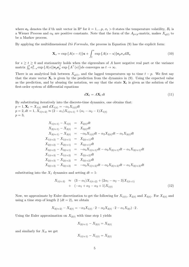
There is an analytical link between Xq(t), and the lagged temperatures up to time t − p. We first saythat the state vector Xt is given by the prediction from the dynamics in (9). Using the expected valueas the prediction, and by abusing the notation, we say that the state Xt is given as the solution of thefirst-order system of differential equations

dXt = AXt dt (11)

By substituting iteratively into the discrete-time dynamics, one obtains that:p = 1,Xt = X1(t) and dX1(t) = −α1X1(t)dtp = 2, dt = 1, X1(t+2) ≈ (2− α1)X1(t+1) + (α1 − α2 − 1)X1(t)

p = 3,

X1(t+1) −X1(t) = X2(t)dt

X2(t+1) −X2(t) = X3(t)dt

X3(t+1) −X3(t) = −α3X1(t)dt− α2X2(t)dt− α1X3(t)dt

X1(t+2) −X1(t+1) = X2(t+1)dt

X2(t+2) −X2(t+1) = X3(t+1)dt

X3(t+2) −X3(t+1) = −α3X1(t+1)dt− α2X2(t+1)dt− α1X3(t+1)dt

X1(t+3) −X1(t+2) = X2(t+2)dt

X2(t+3) −X2(t+2) = X3(t+2)dt

X3(t+3) −X3(t+2) = −α3X1(t+2)dt− α2X2(t+2)dt− α1X3(t+2)dt

substituting into the X1 dynamics and setting dt = 1:

X1(t+3) ≈ (3− α1)X1(t+2) + (2α1 − α2 − 3)X1(t+1)

+ (−α1 + α2 − α3 + 1)X1(t) (12)

Now, we approximate by Euler discretization to get the following for X1(t), X2(t) and X3(t). For X3(t) andusing a time step of length 2 (dt = 2), we obtain

X3(t+2) −X3(t) = −α3X1(t) · 2− α2X2(t) · 2− α1X3(t) · 2 .

Using the Euler approximation on X2(t) with time step 1 yields

X2(t+1) −X2(t) = X3(t)

and similarly for X1t we getX1(t+1) −X1(t) = X2(t)

5

andX1(t+2) −X1(t+1) = X2(t+1)

Hence, inserting in the approximation of X3(t) we find

X3(t+2) = (1− 2α1 + 2α2 − 2α3)X1(t) + (4α1 − 2α2 − 2)X1(t+1) + (1− 2α1)X1(t+2) (13)

Thus, we see that we can recover the state of X3(t) by inserting X1(t) = Tt−Λt at times t, t− 1 and t− 2.Next, we have

X2(t+2) −X2(t+1) = X3(t+1)

which implies, using the recursion on X3(t+2) in Equation (13)

X2(t+2) = X2(t+1) + (1− 2α1 + 2α2 − 2α3)X1(t−1) − (4α1 − 2α2 − 2)X1(t) + (1− 2α1)X1(t+1) .

Inserting for X2(t+1), we get

X2(t+2) = X1(t+2) − 2α1X1(t+1) + (−2 + 4α1 − 2α2)X1(t) + (1− 2α1 + 2α2 − 2α3)X1(t−1) (14)

We see that X2(t+2) can be recovered by the temperature observation at times t + 2, t + 1, t and t − 1.Finally, the state of X1(t) is obviously simply today’s temperature less its seasonal state.

4 Temperature futures pricing

As temperature is not a tradable asset in the market place, no replication arguments hold for any tem-perature futures and incompleteness of the market follows. In this context all equivalent measures Q willbe risk-neutral probabilities. We assume the existence of a pricing measure Q, which can be parametrizedand complete the market, Karatzas and Shreve (2001). For that, we pin down an equivalent measureQ = Qθt to compute the arbitrage free price of a temperature future:

F(t,τ1,τ2) = EQθt [Y (Tt)|Ft] (15)

with Y (Tt) being the payoff from the temperature index (CAT, HDD, CDD indices) and θt denotes thetime dependent market price of risk (MPR). The risk adjusted probability measure can be retrieved viaGirsanov’s theorem, by establishing:

Bθt = Bt −

∫ t

0θudu (16)

Bθt is a Brownian motion for any time before the end of the trading time (t ≤ τmax) and a martingale under

Qθt . Here the market price of risk (MPR) θt = θ is as a real valued, bounded and piecewise continuousfunction. Under Qθ, the temperature dynamics of (10) become

dXt = (AXt + epσtθt)dt+ epσtdBθt (17)

with explicit dynamics, for s ≥ t ≥ 0:

Xs = exp A(s− t)x +

∫ s

texp A(s− u)epσuθudu

+

∫ s

texp A(s− u)epσudBθ

u (18)

6

From Theorem 4.2 (page 12) in Karatzas and Shreve (2001) we can parametrize the market price of riskθt and relate it to the risk premium for traded assets (as WD are indeed tradable assets) by the equation

µt + δt − rt = σtθt (19)

where µt is the mean rate of return process, δt defines a dividend rate process, σt denotes the volatilityprocess and rt determines the risk-free interest rate process of the traded asset. In other words, the riskpremium is the compensation, in terms of mean growth rate, for taking additional risk when investing inthe traded asset. Assuming that δt = 0, a sufficient parametrization of the MPR is setting θt = (µt−rt)/σtto make the discounted asset prices martingales. We later relax that assumption, by considering the timedependent market price of risk.

4.1 CAT Futures and Options

Following Equation (15) and using Fubini-Tonelli, the risk neutral price of a future based on a CAT indexunder Qθ is defined as:

FCAT (t,τ1,τ2) = EQθ[∫ τ2

τ1

Tsds|Ft]

(20)

For contracts whose trading date is earlier than the temperature measurement period, i.e. 0 ≤ t ≤ τ1 < τ2,Benth et al. (2007) calculate the future price explicitly by inserting the temperature model (7) into (20):

FCAT (t,τ1,τ2) =

∫ τ2

τ1

Λudu+ at,τ1,τ2Xt +

∫ τ1

tθuσuat,τ1,τ2epdu

+

∫ τ2

τ1

θuσue>1 A−1 [exp A(τ2 − u) − Ip] epdu (21)

with at,τ1,τ2 = e>1 A−1 [exp A(τ2 − t) − exp A(τ1 − t)] and p × p identity matrix Ip. While for CAT

futures traded between the measurement period i.e. τ1 ≤ t < τ2, the risk neutral price is:

FCAT (t, τ1, τ2) = EQθ[∫ t

τ1

Tsds|Ft]

+ EQθ[∫ τ2

tTsds|Ft

]= EQθ

[∫ t

τ1

Tsds|Ft]

+

∫ τ2

tΛudu+ at,t,τ2Xt

+

∫ τ2

tθuσue

>1 A−1 [exp A(τ2 − u) − Ip] epdu

where at,t,τ2 = e>1 A−1 [exp A(τ2 − t) − Ip]. Since the expected value of the temperature from τ1 to t

is already known, this time the future price consists on a random and a deterministic part. Details ofthe proof can be found in Benth, Saltyte Benth and Koekebakker (2008). Note that the CAT futuresprice is given by the aggregated mean temperature (seasonality) over the measurement period plus amean reversion weighted dependency on Xt, which is depending on the temperature of previous daysTt−k, k ≤ p. The last two terms smooth the market price of risk over the period from the trading date tto the end of the measurement period τ2, with a change happening in time τ1. Similar results hold forthe C24AT index futures.

Note that that only coordinate of Xt that has a has a random component dBθ is Xpt, hence the dynamicsunder Qθ of FCAT (t, τ1, τ2) is:

dFCAT (t, τ1, τ2) = σtat,τ1,τ2epdBθt

7

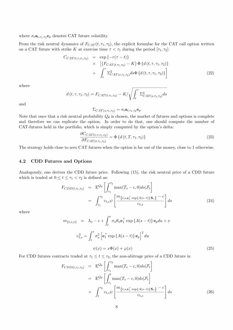
where σtat,τ1,τ2ep denotes CAT future volatility.

From the risk neutral dynamics of FCAT (t, τ1, τ2), the explicit formulae for the CAT call option writtenon a CAT future with strike K at exercise time τ < τ1 during the period [τ1, τ2]:

CCAT (t,τ,τ1,τ2) = exp −r(τ − t)×

[(FCAT (t,τ1,τ2) −K

)Φ d (t, τ, τ1, τ2)

+

∫ τ

tΣ2CAT (s,τ1,τ2)dsΦ d (t, τ, τ1, τ2)

](22)

where

d (t, τ, τ1, τ2) = FCAT (t,τ1,τ2) −K/

√∫ τ

tΣ2CAT (s,τ1,τ2)ds

andΣCAT (s,τ1,τ2) = σtat,τ1,τ2ep

Note that once that a risk neutral probability Qθ is chosen, the market of futures and options is completeand therefore we can replicate the option. In order to do that, one should compute the number ofCAT-futures held in the portfolio, which is simply computed by the option’s delta:

∂CCAT (t,τ,τ1,τ2)

∂FCAT (t,τ1,τ2)= Φ d (t, T, τ1, τ2) (23)

The strategy holds close to zero CAT futures when the option is far out of the money, close to 1 otherwise.

4.2 CDD Futures and Options

Analogously, one derives the CDD future price. Following (15), the risk neutral price of a CDD futurewhich is traded at 0 ≤ t ≤ τ1 < τ2 is defined as:

FCDD(t,τ1,τ2) = EQθ[∫ τ2

τ1

max(Ts − c, 0)ds|Ft]

=

∫ τ2

τ1

υt,sψ

[mt,s,e>1 expA(s−t)Xt − c

υt,s

]ds (24)

where

mt,s,x = Λs − c+

∫ s

tσuθue

>1 exp A(s− t) epdu+ x

υ2t,s =

∫ s

tσ2u

[e>1 exp A(s− t) ep

]2du

ψ(x) = xΦ(x) + ϕ(x) (25)

For CDD futures contracts traded at τ1 ≤ t ≤ τ2, the non-abitrage price of a CDD future is:

FCDD(t,τ1,τ2) = EQθ[∫ τ2

τ1


= EQθ[∫ t

τ1


+

∫ τ2

tυt,sψ


υt,s

]ds (26)

8

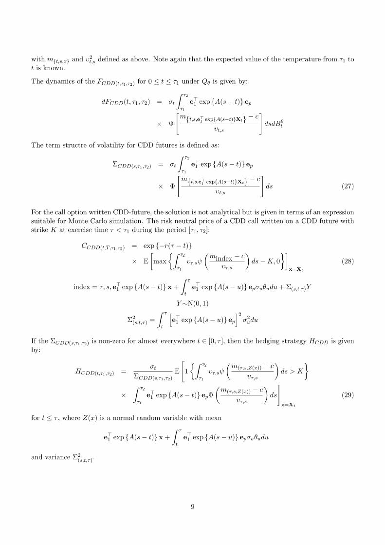
with mt,s,x and υ2t,s defined as above. Note again that the expected value of the temperature from τ1 to

t is known.

The dynamics of the FCDD(t,τ1,τ2) for 0 ≤ t ≤ τ1 under Qθ is given by:

dFCDD(t, τ1, τ2) = σt

∫ τ2

τ1

e>1 exp A(s− t) ep

× Φ


υt,s

]dsdBθ

t

The term structre of volatility for CDD futures is defined as:

ΣCDD(s,τ1,τ2) = σt

∫ τ2

τ1

e>1 exp A(s− t) ep

× Φ


υt,s

]ds (27)

For the call option written CDD-future, the solution is not analytical but is given in terms of an expressionsuitable for Monte Carlo simulation. The risk neutral price of a CDD call written on a CDD future withstrike K at exercise time τ < τ1 during the period [τ1, τ2]:

CCDD(t,T,τ1,τ2) = exp −r(τ − t)

× E

[max

∫ τ2

τ1

υτ,sψ

(mindex − c

υτ,s

)ds−K, 0

]x=Xt

(28)

index = τ, s, e>1 exp A(s− t)x +

∫ τ

te>1 exp A(s− u) epσuθudu+ Σ(s,t,τ)Y

Y∼N(0, 1)

Σ2(s,t,τ) =

∫ τ

t

[e>1 exp A(s− u) ep

]2σ2udu

If the ΣCDD(s,τ1,τ2) is non-zero for almost everywhere t ∈ [0, τ ], then the hedging strategy HCDD is givenby:

HCDD(t,τ1,τ2) =σt

ΣCDD(s,τ1,τ2)E

[1

∫ τ2

τ1

υτ,sψ

(m(τ,s,Z(x)) − c

υτ,s

)ds > K

×∫ τ2

τ1

e>1 exp A(s− t) epΦ(m(τ,s,Z(x)) − c

υτ,s

)ds

]x=Xt

(29)

for t ≤ τ , where Z(x) is a normal random variable with mean

e>1 exp A(s− t)x +

∫ τ

te>1 exp A(s− u) epσuθudu

and variance Σ2(s,t,τ).

9

4.3 Infering the market price of temperature risk

In the weather derivative market there is obviously the question of choosing the right price among possiblearbitrage free prices. For pricing nontradable assets one essentially needs to incorporate the market priceof risk (MPR), which is an important parameter of the associated equivalent martingale measures usedto price and hedge weather futures/options in the market. MPR can be calibrated from data and therebyusing the market to pin down the price of the temperature derivative. Once we know the MPR fortemperature futures, then we know the MPR for options.

By inverting (21), given observed prices, θt is inferred for contracts with trading date t ≤ τ1 < τ2. Settingθit as a constant for each of the i contract, with i = 1 . . . 7, θit is estimated via:

arg minθit

(FAAT (t,τ i1,τ

i2) −

∫ τ i2

τ i1

Λudu− at,τ i1,τ i2Xt

− θit

∫ τ i1

tσuat,τ i1,τ i2

epdu

+

∫ τ i2

τ i1

σue>1 A−1[exp

A(τ i2 − u)

− Ip

]epdu

)2

(30)

A simpler parametrization of θt is to assume that it is constant for all maturities. We therefore estimatethis constant θt for all contracts with t ≤ τ i1 < τ i2, i = 1, · · · , 7 as follows:

arg minθt

Σ7i=1

(FCAT (t,τ i1,τ

i2) −

∫ τ i2

τ i1


− θt

∫ τ i1

tσuat,τ i1,τ i2

epdu

+

∫ τ i2

τ i1

σue>1 A−1[exp

A(τ i2 − u)

− Ip

]epdu

)2

Assuming now that, instead of one constant market price of risk per trading day, we have a step functionwith jump θt = I (u ≤ ξ) θ1

t + I (u > ξ) θ2t with jump point ξ (take e.g. the first 150 days before the

beginning of the measurement period). Then we estimate θt for contracts with t ≤ τ i1 < τ i2, i = 1, · · · , 7by:

f(ξ) = arg minθ1t ,θ

2t

Σ7i=1

(FCAT (t,τ i1,τ

i2) −

∫ τ i2

τ i1


− θ1t

∫ τ i1

tI (u ≤ ξ) σuat,τ i1,τ i2epdu

+

∫ τ i2

τ i1

I (u ≤ ξ) σue>1 A−1[exp

A(τ i2 − u)

− Ip

]epdu

− θ2t

∫ τ i1

tI (u > ξ) σuat,τ i1,τ i2

epdu

+

∫ τ i2

τ i1

I (u > ξ) σue>1 A−1[exp

A(τ i2 − u)

− Ip

]epdu

)2

10

City Period a0 a1 a2 a3Tokyo 19730101-20081231 15.76 7.82e-05 10.35 -149.53Osaka 19730101-20081231 15.54 1.28e-04 11.50 -150.54Beijing 19730101-20081231 11.97 1.18e-04 14.91 -165.51Taipei 19920101-20090806 23.21 1.68e-03 6.78 -154.02

Table 2: Seasonality estimates of daily average temperatures in Asia. Data source: Bloomberg

Generalising the previous piecewise continuous function, the (inverse) problem of determining θt witht ≤ τ i1 < τ i2, i = 1, · · · 7 can be formulated via a series expansion for θt:

arg minγk

Σ7i=1

(FAAT (t,τ i1,τ

i2) −

∫ τ i2

τ i1

Λudu− at,τ1i ,τi2Xt

−∫ τ i1

t

K∑k=1

γkhk(ui)σui at,τ1,τ2epdui

−∫ τ i2

τ i1

K∑k=1

γkhk(ui)σuie>1 A−1[exp

A(τ i2 − ui)

− Ip] epdui

)2

(31)

where hk(ui) is a vector of known basis functions and γk defines the coefficients. Here hk(ui) may denotea spline basis for example. Hardle and Lopez Cabrera (2009) show additional methods about how toinfere the MPR.

5 Asian temperature derivatives

5.1 Asian temperature dynamics

We turn now to the analysis of the weather dynamics for Tokyo, Osaka, Beijing and Taipei daily tem-perature data. The temperature data were obtained from the Tokyo Narita International Airport, OsakaKansai International Airport and Bloomberg. We consider recordings of daily average temperatures from19730101 - 20090604. In all studied data, a linear trend was not detectable but a clear seasonal patternemerged. Figure 1 shows 8 years of daily average temperatures and the least squares fitted seasonalfunction with trend:

Λt = a0 + a1t+ a2cos

2π(t− a3)

365

(32)

The estimated coefficients are displayed in Table 2.

The low order polynomial deterministic trend smooths the seasonal pattern and makes the model to beparsimonius. The coefficient a0 can be interpretated as the average temperature, while a1 as the globalwarming trend component. In most of the Asian cases, as expected, the low temperatures are observedin the winter and high temperatures in the summer.

After removing the seasonality in (32) from the daily average temperatures,

Xt = Tt − Λt (33)

11

1973 1979 1985 1991 1997 2003 20080

10

20

30

Time

Tem

per

atu

re in

To

kyo

20010101 20030101 20050101 20070101 200901010

10

20

30

Time

Tem

per

atu

re in

To

kyo

1973 1979 1985 1991 1997 2003 2008

0

10

20

30

Time

Tem

per

atu

re in

Osa

ka

20010101 20030101 20050101 20070101 20090101

0

10

20

30

Time

Tem

per

atu

re in

Osa

ka

1973 1979 1985 1991 1997 2003 2008

−10

0

10

20

30

Time

Tem

pera

ture

inB

eijin

g

20010101 20030101 20050101 20070101 20081231

−10

0

10

20

30

Time

Tem

pera

ture

inB

eijin

g

20010101 20040101 20070101 2008123110

20

30

Time

Tem

per

atu

re in

Tai

pei

Figure 1: Seasonality effect and daily average temperatures for Tokyo Narita International Airport, Osaka Kansai Interna-tional Airport, Beijing and Taipei.

AsianWeather1

12

City τ(p-value) k(p-value)

Tokyo -56.29(< 0.01) 0.091(< 0.1)Osaka -17.86(< 0.01) 0.138(< 0.1)Beijing -20.40(< 0.01) 0.094(< 0.1)Taipei -33.21(< 0.01) 0.067(< 0.1)

Table 3: Stationarity tests.

every every every every everyYear 3 years 6 years 9 years 12 years 18 years

73-75 AR(1) 2*AR(3) 3*AR(3) 4*AR(8)* 6*AR(9)*76-78 AR(1)79-81 AR(1) 2*AR(8)*82-84 AR(8)* 3*AR(9)*85-87 AR(1) 2*AR(3) 4*AR(3)88-90 AR(1)91-93 AR(1) 2*AR(3) 3*AR(3) 6*AR(3)94-96 AR(1)97-99 AR(1) 2*AR(1) 4*AR(3)00-02 AR(1) 3*AR(3)03-05 AR(3) 2*AR(3)06-09 AR(1)

Table 4: Tokyo Moving window for AR, * denotes instability

we check whether Xt is a stationary process I(0). In order to do that, we apply the Augmented Dickey-Fuller test (ADF) (1 − L)X = c1 + µt + τLX + α1(1 − L)LX + . . . αp(1 − L)LpX + εt, where p is thenumber of lags by which the regression is augmented to get residuals free of autocorrelation. Under H0

(unit root), τ should be zero. Therefore the test statistic of the OLS estimator of τ is applicable. If thenull hypothesis H0 (τ = 0) is rejected then Xt is a stationary process I(0).

Stationarity can also be verified by using the KPSS Test: Xt = c+ µt+ k∑t

i=1 ξi + εt with stationary εtand iid ξt with an expected value 0 and variance 1. If H0 : k = 0 is accepted then the process is stationary.The estimates of τ and k of the previuos stationarity tests are illustrated in Table 3, indicating that thestationarity is achieved.

The Partial Autocorrelation Function (PACF) of (33) suggests that higher order autoregressive modelsAR(p), p > 1 are suitable for modelling the time evolution of Asia temperatures after removing seasonality,see Figure 2.

The covariance stationarity dynamics were captured using autoregressive lags over different year-lengthsmoving windows, as it is denoted in Table 4 and Table 5 for the case of Tokyo and Osaka. The autore-gressive models showed, for larger length periods, higher order p and sometimes lack of stability (AR *),i.e. the eigenvalues of matrix A (8) had positive real part. Since local estimates of the a fitted seasonalvariation σt with GARCH models captures long memory affects and assuming that it shocks temperatureresiduals in the same way over different length periods, the autoregressive model AR(3) was therefore cho-sen. p = 3 is also confirmed by the Akaike and Schwarz information criteria for each city. The coefficientsof the fitted autoregressive process

Xt+p =

p∑i=1

βiXt+p−i + σtεt (34)

and their corresponding are CAR(3)-parameters displayed in Table 6. The stationarity condition isfulfilled since the eigenvalues of A have negative real parts. The element components of the matrix A (8)do not change over time, this makes the process stable.

13

0 5 10 15 20 25 30 35 40 45 50−0.1

0

0.1

0.2

0.3

0.4

0.5

0.6

0.7

Lags

Par

tial A

utoc

orre

latio

n fu

nctio

n

PACF, alpha=0.05

0 5 10 15 20 25 30 35 40 45 50−0.1

0

0.1

0.2

0.3

0.4

0.5

0.6

0.7

Lags

Par

tial A

utoc

orre

latio

n fu

nctio

n

PACF, alpha=0.05

0 5 10 15 20 25 30 35 40 45 50−0.1

0

0.1

0.2

0.3

0.4

0.5

0.6

0.7

0.8

Lags

Par

tial A

utoc

orre

latio

n fu

nctio

n

PACF, alpha=0.05

0 5 10 15 20 25 30 35 40 45 50−0.2

−0.1

0

0.1

0.2

0.3

0.4

0.5

0.6

0.7

Lags

Par

tial A

utoc

orre

latio

n fu

nctio

n

PACF, alpha=0.05

Figure 2: Partial autocorrelation function (PACF) for Tokyo (upper left), Osaka (upper right), Beijing (lower left), Taipei(lower right)

AsianWeather2

every every every every everyYear 3 years 6 years 9 years 12 years 18 years

73-75 AR(1) 2*AR(3) 3*AR(3) 4*AR(3) 6*AR(6)*76-78 AR(3)79-81 AR(3) 2*AR(3)82-84 AR(2) 3*AR(3)85-87 AR(3) 2*AR(3) 4*AR(6)*88-90 AR(3)91-93 AR(3) 2*AR(3) 3*AR(6)* 6*AR(7)*94-96 AR(1)97-99 AR(2) 2*AR(2) 4*AR(7)*00-02 AR(1) 3*AR(3)03-05 AR(3) 2*AR(3)06-09 AR(1)

Table 5: Osaka Moving window for AR, * denotes instability.

14

Coefficient Tokyo(p=3) Osaka(p=3) Beijing(p=3) Taipei(p=3)AR β1 0.668 0.748 0.741 0.808

β2 -0.069 -0.143 -0.071 -0.228β3 -0.079 -0.079 0.071 0.063

CAR α1 -2.332 -2.252 -2.259 -2.192α2 1.733 -1.647 -1.589 -1.612α3 -0.480 -0.474 -0.259 -0.357

Eigenvalues real part of λ1 -1.257 -1.221 -0.231 -0.396real part of λ2,3 -0.537 -0.515 -1.013 -0.8976

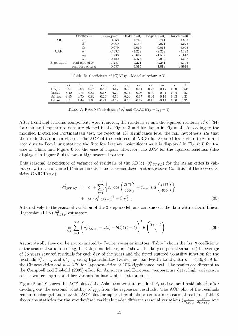
Table 6: Coefficients of (C)AR(p), Model selection: AIC.

c1 c2 c3 c4 c5 c6 c7 c8 c9 α βTokyo 3.91 -0.08 0.74 -0.70 -0.37 -0.13 -0.14 0.28 -0.15 0.09 0.50Osaka 3.40 0.76 0.81 -0.58 -0.29 -0.17 -0.07 0.01 -0.04 0.04 0.52Beijing 3.95 0.70 0.82 -0.26 -0.50 -0.20 -0.17 -0.05 0.10 0.03 0.33Taipei 3.54 1.49 1.62 -0.41 -0.19 0.03 -0.18 -0.11 -0.16 0.06 0.33

Table 7: First 9 Coefficients of σ2t and GARCH(p = 1, q = 1).

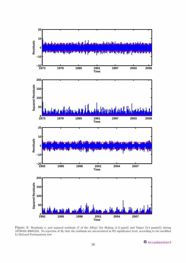
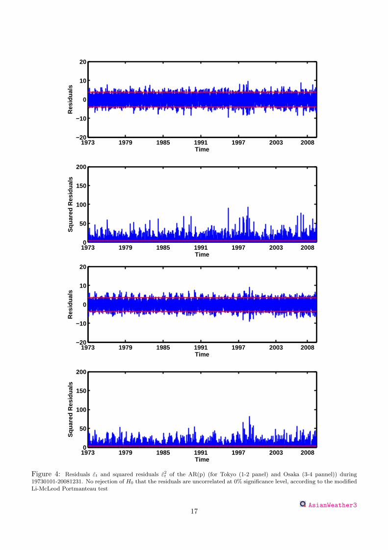
After trend and seasonal components were removed, the residuals εt and the squared residuals ε2t of (34)

for Chinese temperature data are plotted in the Figure 3 and for Japan in Figure 4. According to themodified Li-McLeod Portmanteau test, we reject at 1% significance level the null hypothesis H0 thatthe residuals are uncorrelated. The ACF of the residuals of AR(3) for Asian cities is close to zero andaccording to Box-Ljung statistic the first few lags are insignificant as it is displayed in Figure 5 for thecase of China and Figure 6 for the case of Japan. However, the ACF for the squared residuals (alsodisplayed in Figure 5, 6) shows a high seasonal pattern.

This seasonal dependence of variance of residuals of the AR(3) (σ2t,FTSG) for the Asian cities is cali-

brated with a truncanted Fourier function and a Generalized Autoregressive Conditional Heteroscedas-ticity GARCH(p,q):

σ2t,FTSG = c1 +

16∑i=1

c2i cos

(2iπt

365

)+ c2i+1 sin

(2iπt

365

)+ α1(σ2

t−1εt−1)2 + β1σ2t−1 (35)

Alternatively to the seasonal variation of the 2 step model, one can smooth the data with a Local LinearRegression (LLN) σ2

t,LLR estimator:

mina,b

365∑i=1

(σ2t,LLR,i − a(t)− b(t)(Ti − t)

)2

K

(Ti − th

)(36)

Asympotically they can be approximated by Fourier series estimators. Table 7 shows the first 9 coefficientsof the seasonal variation using the 2 steps model. Figure 7 shows the daily empirical variance (the averageof 35 years squared residuals for each day of the year) and the fitted squared volatility function for theresiduals σ2

t,FTSG and σ2t,LLR using Epanechnikov Kernel und bandwidth bandwidth h = 4.49, 4.49 for

the Chinese cities and h = 3.79 for Japanese cities at 10% significance level. The results are different tothe Campbell and Diebold (2005) effect for American and European temperature data, high variance inearlier winter - spring and low variance in late winter - late summer.

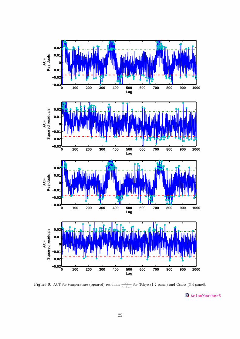
Figure 8 and 9 shows the ACF plot of the Asian temperature residuals εt and squared residuals ε2t , after

dividing out the seasonal volatility σ2t,LLR from the regression residuals. The ACF plot of the residuals

remain unchanged and now the ACF plot for squared residuals presents a non-seasonal pattern. Table 8shows the statistics for the standardized residuals under different seasonal variations ( εt

σt,FTS, εtσt,FTSG

and

15

1973 1979 1985 1991 1997 2003 2008−20

−10

0

10

20

Time

Res

idua

ls

1973 1979 1985 1991 1997 2003 20080

50

100

150

200

Time

Squ

ared

Res

idua

ls

1992 1995 1998 2001 2004 2007−20

−10

0

10

20

Time

Res

idua

ls

1992 1995 1998 2001 2004 20070

50

100

150

200

Time

Squ

ared

Res

idua

ls

Figure 3: Residuals εt and squared residuals ε2t of the AR(p) (for Beijing (1-2 panel) and Taipei (3-4 pannel)) during19730101-20081231. No rejection of H0 that the residuals are uncorrelated at 0% significance level, according to the modifiedLi-McLeod Portmanteau test

AsianWeather316

1973 1979 1985 1991 1997 2003 2008−20

−10

0

10

20

Time

Res

idua

ls

1973 1979 1985 1991 1997 2003 20080

50

100

150

200

Time

Squ

ared

Res

idua

ls

1973 1979 1985 1991 1997 2003 2008−20

−10

0

10

20

Time

Res

idua

ls

1973 1979 1985 1991 1997 2003 20080

50

100

150

200

Time

Squ

ared

Res

idua

ls

Figure 4: Residuals εt and squared residuals ε2t of the AR(p) (for Tokyo (1-2 panel) and Osaka (3-4 pannel)) during19730101-20081231. No rejection of H0 that the residuals are uncorrelated at 0% significance level, according to the modifiedLi-McLeod Portmanteau test

AsianWeather317

0 100 200 300 400 500 600 700 800 900 1000

−0.02

0

0.02

0.04A

CF

Res

idua

ls

Lag

0 100 200 300 400 500 600 700 800 900 1000

−0.02

0

0.02

0.04

0.06

0.08

AC

FS

quar

ed r

esid

uals

Lag

0 100 200 300 400 500 600 700 800 900 1.000

−0.02

0

0.02

0.04

AC

FR

esid

uals

Lag

0 100 200 300 400 500 600 700 800 900 1.000

−0.1

−0.05

0

0.05

0.1

AC

FS

quar

ed r

esid

uals

Lag

Figure 5: ACF for residuals εt and squared residuals ε2t of the AR(p) of the AR(p) (for Beijing (1-2 panel) and Taipei (3-4pannel)) during 19730101-20081231

AsianWeather4

18

0 100 200 300 400 500 600 700 800 900 1000

−0.02

0

0.02

0.04A

CF

Res

idua

ls

Lag

0 100 200 300 400 500 600 700 800 900 1000

−0.02

0

0.02

0.04

0.06

0.08

AC

FS

quar

ed r

esid

uals

Lag

0 100 200 300 400 500 600 700 800 900 1000

−0.02

0

0.02

0.04

AC

FR

esid

uals

Lag

0 100 200 300 400 500 600 700 800 900 1000

−0.02

0

0.02

0.04

0.06

0.08

AC

FS

quar

ed r

esid

uals

Lag

Figure 6: ACF for residuals εt and squared residuals ε2t of the AR(p) of the AR(p) (for Tokyo (1-2 panel) and Osaka (3-4panel)) during 19730101-20081231

AsianWeather4

19

Jan Feb Mar Apr May Jun Jul Aug Sep Oct Nov Dec1

2

3

4

5

6

7

8

Time

Sea

son

al V

aria

nce

Kernel v.s. Fourier


2

4

6

8

10

12

Time

Sea

son

al V

aria

nce

Kernel v.s. Fourier


2

3

4

5

6

7

8

9

Time

Sea

son

al V

aria

nce

Kernel v.s. Fourier


2

3

4

5

6

7

8

Time

Sea

son

al V

aria

nce

Kernel v.s. Fourier

Figure 7: Daily empirical variance, σ2t,FTSG,σ2

t,LLR for Beijing (upper left), Taipei (upper right), Tokyo (lower left), Osaka(lower right)

AsianWeather5

εtσt,LLR

). The estimator of the seasonal variation with local linear regression was the closer to the normal

residuals. The acceptance of the null hyptohesis H0 of normality is at 1% significance level.

The log Kernel smoothing density estimate against a log Normal Kernel evaluated at 100 equally spacedpoints for Asian temperature residuals has been plotted in Figure (10) to verify if residuals becomenormally distributed. The seasonal variation modelled with a GARCH (1,1) and by the local linearregression are adequately capturing the intertemporal dependencies in daily temperature.

5.2 Pricing Asian futures

In this section, using Equation (30) and (31) but for C24AT index futures, we infered the market price ofrisk for C24AT Asian temperature derivatives as Hardle and Lopez Cabrera (2009) did for Berlin monthlyCAT futures. Table 9 shows the replication of the observed Tokyo C24AT index futures prices tradedin Bloomberg on 20090130, using the constant MPR for each contract per trading day and the timedependent MPR using cubic polynomials with number of knots equal to the number of traded contracts(7). One can notice that the C24AT index futures for Tokyo are underpriced when the MPR is equal tozero. From (21) for C24AT index futures, we observe that a high proportion of the price value comes fromthe seasonal exposure, showing high CAT temperature futures prices from June to August and low pricesfrom November to February. The influence of the temperature variation σt can be clearly reflected in thebehaviour of the MPR. For both parametrization, MPR is close to zero far from measurement period andit jumps when it is getting closed to it. This phenomena is also related to the Samuelson effect, wherethe CAT volatility for each contract is getting closed to zero when the time to measurement period islarge. C24AT index futures future prices with constant MPR estimate per contract per trading day full

20

0 100 200 300 400 500 600 700 800 900 1000−0.03

−0.02

−0.01

0

0.01

0.02

Lag

AC

FR

esid

uals

0 100 200 300 400 500 600 700 800 900 1000−0.03

−0.02

−0.01

0

0.01

0.02

Lag

AC

FS

quar

ed r

esid

uals

0 100 200 300 400 500 600 700 800 900 1000−0.03

−0.02

−0.01

0

0.01

0.02

Lag

AC

FR

esid

uals

0 100 200 300 400 500 600 700 800 900 1000−0.03

−0.02

−0.01

0

0.01

0.02

Lag

AC

FS

quar

ed r

esid

uals

Figure 8: ACF for temperature (squared) residuals εtσt,LLR

for Beijing (1-2 panel)and Taipei (3-4 pannel).

AsianWeather6

21

0 100 200 300 400 500 600 700 800 900 1000−0.03

−0.02

−0.01

0

0.01

0.02

Lag

AC

FR

esid

uals

0 100 200 300 400 500 600 700 800 900 1000−0.03

−0.02

−0.01

0

0.01

0.02

Lag

AC

FS

quar

ed r

esid

uals

0 100 200 300 400 500 600 700 800 900 1000−0.03

−0.02

−0.01

0

0.01

0.02

Lag

AC

FR

esid

uals

0 100 200 300 400 500 600 700 800 900 1000−0.03

−0.02

−0.01

0

0.01

0.02

Lag

AC

FS

quar

ed r

esid

uals

Figure 9: ACF for temperature (squared) residuals εtσt,LLR

for Tokyo (1-2 panel) and Osaka (3-4 panel).

AsianWeather6

22

City εtσt,FTS

εtσt,FTSG

εtσt,LLR

Tokyo Jarque Bera 158.00 127.23 114.50Kurtosis 3.46 3.39 3.40Skewness -0.15 -0.11 -0.12

Osaka Jarque Bera 129.12 119.71 105.02Kurtosis 3.39 3.35 3.33Skewness -0.15 -0.14 -0.14

Beijing Jarque Bera 234.07 223.67 226.09Kurtosis 3.28 3.27 3.25Skewness -0.29 -0.29 -0.29

Taipei Jarque Bera 201.09 198.40 184.17Kurtosis 3.36 3.32 3.3Skewness -0.39 -0.39 -0.39

Table 8: Statistics of the Asian temperature residuals εt and squared residuals ε2t , after dividing out the seasonal volatilityσ2t,LLR from the regression residuals

−5 0 50

0.1

0.2

0.3

0.4

0.5

−5 0 5−14

−12

−10

−8

−6

−4

−2

0

−5 0 50

0.1

0.2

0.3

0.4

0.5

−5 0 5−14

−12

−10

−8

−6

−4

−2

0

−5 0 50

0.1

0.2

0.3

0.4

0.5

−5 0 5−14

−12

−10

−8

−6

−4

−2

0

−5 0 50

0.1

0.2

0.3

0.4

0.5

−5 0 5−14

−12

−10

−8

−6

−4

−2

0

−5 0 50

0.1

0.2

0.3

0.4

0.5

−5 0 5−14

−12

−10

−8

−6

−4

−2

0

−5 0 50

0.1

0.2

0.3

0.4

0.5

−5 0 5−14

−12

−10

−8

−6

−4

−2

0

−5 0 50

0.1

0.2

0.3

0.4

0.5

−5 0 5−14

−12

−10

−8

−6

−4

−2

0

−5 0 50

0.1

0.2

0.3

0.4

0.5

−5 0 5−14

−12

−10

−8

−6

−4

−2

0

Figure 10: Log of Kernel smoothing density estimate vs Log of Normal Kernel for εtσt,LLR

(upper) and εtσt,FTSG

(lower) of

Tokyo (left), Osaka (left middle), Beijing (right middle), Taipei (right)

AsianWeather7

23

City Code FC24ATBloomberg FC24AT,θ0tFC24AT,θit

FC24AT,θ

splt

Tokyo J9 450.000 452.125 448.124 461.213K9 592.000 630.895 592.000 640.744

Osaka J9 460.000 456.498 459.149 -K9 627.000 663.823 624.762 -

Table 9: Tokyo & Osaka C24AT future prices estimates on 20090130 from different MPR parametrization methods.

replicate the Bloomberg estimates and pricing deviations are smoothed over time when the estimationsuse smoothed MPRs. Positive (negative) MPR contributes positively (negatively) to future prices, leadingto larger (smaller) estimation values than the real prices.

The Chicago Mercantile exchange does not carry out trade CDD futures for Asia, however one can usethe estimates of the smoothed MPR of CAT (C24AT) futures in (21) to price CDD futures. From theHDD-CDD parity (5), one can estimate HDD futures and compare them with real data.

Since C24AT futures are indeed tradable assets, a simple and sufficient parametrization of the MPR tomake the discounted asset prices martingales is setting θt = (µt − rt)/σt. In order to see which of thecomponents (µt − rt or σt) contributes more to the variation of the MPR, the seasonal effect that theMPR θt presents was related with the seasonal variation σt of the underlying process. In this case, therelationship between θt and σt is well defined given by the deterministic form of σt(σt,FTSG, σt,LLR) inthe temperature process.

First, using different trading day samples, the average of the calibrated θit over the period [τ1, τ2] wasestimated as:

θi[τ1,τ2] =1

Tτ1,τ2 − tτ1,τ2

Tτ1,τ2∑t=tτ1,τ2

θit,

where t[τ1,τ2] and T[τ1,τ2] indicate the first and the last trade for the contracts with measurement month[τ1, τ2]. Similarly, the variation over the measurement period [τ1, τ2] was defined as:

σ2[τ1,τ2] =

1

τ2 − τ1

τ2∑t=τ1

σ2t .

Then one can conduct a regression model of θiτ1,τ2 on σ2τ1,τ2 . Figure 11 shows the linear and quadratic

regression of the average of the calibrated MPR and σt(σt,FTSG, σt,LLR) of CAT-C24AT Futures withMeasurement Period (MP) in 1 month for Berlin-Essen and Tokyo weather derivative from July 2008to June 2009. The values of θit for contracts on Berlin and Essen were assumed coming from the samepopulation, while for the asian temperature market, Tokyo was the only considered one for being thelargest one. As we expect, the contribution of σt into θt = (µt− rt)/σt gets larger the closer the contractsare to the measurement period. Table 10 shows the coefficients of the parametrization of θit for theGerman and Japanese temperature market. A quadratic regression was fitting more suitable than a linearregression (see R2 coefficients).

The previous findings generally support theoretical results of reverse relation between MPR θτ1,τ2 andseasonal variation σt(σt,FTSG, σt,LLR), indicating that a simple parametrization is possible. Therefore,the MPR for regions without weather derivative markets can be infered by calibration of the data or byknowing the formal dependence of MPR on seasonal variation. We conducted an empirical analysis toweather data in Koahsiung, which is located in the south of China and it is characterized by not havinga formal temperature market, see Figure 12. In a similar way that other Asian cities, a seasonal function

24

3.5 4 4.5 5 5.5 6−0.3

−0.2

−0.1

0

0.1

0.2

average temperature variation in the measurement month

MPR

2.5 3 3.5 4 4.5 5 5.5−0.4

−0.2

0

0.2

0.4

0.6

average temperature variation in the measurement month

MPR

Figure 11: Average of the Calibrated MPR and the Temperature Variation of CAT-C24AT Futures with MeasurementPeriod (MP) in 1 month (Linear, quadratic). Berlin and Essen (left) and Tokyo (right) from July 2008 to June 2009.

AsianWeather8

City Parameters θτ1,τ2 = a+ b · σ2τ1,τ2 θτ1,τ2 = a+ b · σ2

τ1,τ2 + c · σ4τ1,τ2

Berlin- a 0.3714 2.0640Essen b -0.0874 -0.8215

c - 0.0776R2adj 0.4157 0.4902

Tokyo a - 4.08b - -2.19c - 0.28

R2adj - 0.71

Table 10: Parametrization of MPR in terms of seasonal variation for contracts with measurement period of 1 month.

25

i 1 2 3 4 5 6

ci 5.11 -1.34 -0.39 0.61 0.56 0.34

di -162.64 19.56 16.72 28.86 16.63 21.84

Table 11: Coefficients of the seasonal function with trend for Koahsiung

with trend was fitted:

Λt = 24.4 + 16 · 10−5t+3∑i=1

ci · cos

2πi(t− di)

365

+ I(t ∈ ω) ·6∑i=4

ci · cos

2π(i− 4)(t− di)

365

(37)

where I(t ∈ ω) is the indicator function for the months of December, January and February. This formof the seasonal function makes possible to capture the peaks of the temperature in Koahsiung, see upperpanel of Figure 12. The coefficient values of the fitted seasonal function are shown in Table 11.

The fitted AR(p) process to the residuals of Koahsiung by AIC was of degree p = 3, where

β1 = 0.77, β2 = −0.12, β3 = 0.04

and CAR(3) with coefficientsα1 = −2.24, α2 = −1.59, α3 = −0.31

The seasonal volatility fitted with Local Linear Regression (LLR) is plotted in the middle panel of Fig-ure 12, showing high volatility in late winter - late spring and low volatility in early summer - earlywinter. The standardized residuals after removing the seasonal volatility are very closed to normality(kurtosis=3.22, skewness=-0.08, JB=128.74), see lower panel of Figure 12.

For 0 ≤ t ≤ τ1 < τ2, the C24AT Future Contract for Kaohsiung is equal to:

FC24AT (t,τ1,τ2) = EQθ[∫ τ2

τ1

Tsds|Ft]

=

∫ τ2

τ1

Λudu+ at,τ1,τ2Xt +

∫ τ1

t

θτ1,τ2σuat,τ1,τ2epdu

+

∫ τ2

τ1

θτ1,τ2σue>1 A−1 [exp A(τ2 − u) − Ip] epdu (38)

where θτ1,τ2 = 4.08 − 2.19 · σ2τ1,τ2 + 0.028 · σ4

τ1,τ2 , i.e. the formal dependence of MPR on seasonal variation for

C24AT-Tokyo futures. In this case σ2τ1,τ2=1.10, θτ1,τ2=2.01 and FC24AT (20090901,20091027,20091031)=139.60.

The C24AT-Call Option written on a C24AT future with strike K at exercise time τ < τ1 during period [τ1, τ2] isequal to:

CC24AT (t,τ,τ1,τ2) = exp −r(τ − t)×[ (FC24AT (t,τ1,τ2) −K

)Φ d(t, τ, τ1, τ2)

+

∫ τ

t

Σ2C24AT (s,τ1,τ2)

dsΦ d(t, τ, τ1, τ2)],

Table 12 shows the value of the C24AT-Call Option written on a C24AT future with strike price K = 125C, themeasurement period during the 27-31th October 2009 and trading date on 1st. September 2009. The price of theC24AT-Call for Koahsiung decreases when the measurement period is getting closer. This example give us theinsight that by knowing the formal dependence of MPR on seasonal variation, one can infere the MPR for regionswhere weather derivative market does not exist and with that one can price new exotic derivatives. Without doubt,the empirical findings of the MPR need to be further developed to better understand its behaviour.

26

Tokyo

Beijing

Taipei

Osaka

Kaohsiung Kaohsiung Kaohsiung Kaohsiung Kaohsiung Kaohsiung

20010801 20030801 20050801 20070801 20090801

15

20

25

30

Tem

pera

ture

in

°C


1

2

3

4

5

6

Time

Variation

−5 0 50

0.1

0.2

0.3

0.4

0.5

−5 0 5−15

−10

−5

0

Figure 12: Map, Seasonal function with trend (upper), Seasonal volatility function (middle) and Kernel smoothing densityestimate vs Normal Kernel for εt

σt,LLR(lower) for Koahsiung

AsianWeather9

27

Derivative Type Parameters

Index C24ATr 1%t 1. September 2009

Measurement Period 27-31. October 2009Strike 125C

Tick Value 0.01C=U25FC24AT (20090901,20091027,20091031) 139.60

CC24AT (20090901,20090908,20091027,20091031) 12.25CC24AT (20090901,20090915,20091027,20091031) 10.29CC24AT (20090901,20090922,20091027,20091031) 8.69CC24AT (20090901,20090929,20091027,20091031) 7.25

Table 12: C24AT Calls in Koahsiung

6 Conclusion

This paper analyses the pricing of asian weather risk. We apply higher order continuous time autoregressive modelsCAR(3) with seasonal variance for modelling Asian temperature. We modelled the seasonal variation with a GARCHmodel and with a local linear regression in order to achieve normal residuals and with that being able to work in afinancial mathematics context.

From temperature derivative (C24AT) data of the Chicago Mercantile Exchange (CME), the calibration of themarket price of risk is estimated to price new weather derivatives. The MPR for C24AAT temperature derivativesis different from zero, showing a seasonal structure that comes from the seasonal variance of the temperatureprocess. The empirical findings in this paper generally support theoretical results of reverse relation between MPRand variation. Therefore, by knowing the formal dependence of MPR on seasonal variation, one can infere the MPRfor regions where weather derivative market does not exist.

28

References

Alaton, P., Djehiche, B. and Stillberger, D. (2002). On modelling and pricing weather derivatives, Appl. Math.Finance 9(1): 1–20.

Barrieu, P. and El Karoui, N. (2002). Optimal design of weather derivatives, ALGO Research 5(1).

Benth, F. (2003). On arbitrage-free pricing of weather derivatives based on fractional brownian motion., Appl.Math. Finance 10(4): 303–324.

Benth, F. (2004). Option Theory with Stochastic Analysis: An Introduction to Mathematical Finance., SpringerVerlag, Berlin.

Benth, F. and Meyer-Brandis, T. (2009). The information premium for non-storable commodities, Journal of EnergyMarkets 2(3).

Benth, F. and Saltyte Benth, J. (2005). Stochastic modelling of temperature variations with a view towards weatherderivatives., Appl. Math. Finance 12(1): 53–85.

Benth, F., Saltyte Benth, J. and Koekebakker, S. (2007). Putting a price on temperature., Scandinavian Journalof Statistics 34: 746–767.

Benth, F., Saltyte Benth, J. and Koekebakker, S. (2008). Stochastic modelling of electricity and related markets,World Scientific Publishing.

Brody, D., Syroka, J. and Zervos, M. (2002). Dynamical pricing of weather derivatives, Quantit. Finance (3): 189–198.

Campbell, S. and Diebold, F. (2005). Weather forecasting for weather derivatives, American Stat. Assoc.100(469): 6–16.

Cao, M. and Wei, J. (2004). Weather derivatives valuation and market price of weather risk, 24(11): 1065–1089.

CME (2005). An introduction to cme weather products, http://www.vfmarkets.com/pdfs/introweatherfinal.pdf,CME Alternative Investment Products .

Davis, M. (2001). Pricing weather derivatives by marginal value, Quantit. Finance (1): 305–308.

Dornier, F. and Querel, M. (2000). Caution to the wind, Energy Power Risk Management,Weather Risk SpecialReport pp. 30–32.

Hamisultane, H. (2007). Extracting information from the market to price the weather derivatives, ICFAI Journalof Derivatives Markets 4(1): 17–46.

Hardle, W. K. and Lopez Cabrera, B. (2009). Infering the market price of weather risk, SFB649 Working Paper,Humboldt-Universitat zu Berlin .

Horst, U. and Mueller, M. (2007). On the spanning property of risk bonds priced by equilibrium, Mathematics ofOperation Research 32(4): 784–807.

Hull, J. (2006). Option, Future and other Derivatives, Prentice Hall International, New Jersey.

Hung-Hsi, H., Yung-Ming, S. and Pei-Syun, L. (2008). Hdd and cdd option pricing with market price of weatherrisk for taiwan, The Journal of Future Markets 28(8): 790–814.

Ichihara, K. and Kunita, H. (1974). A classification of the second order degenerate elliptic operator and its proba-bilistic characterization, Z. Wahrsch. Verw. Gebiete 30: 235–254.

Jewson, S., Brix, A. and Ziehmann, C. (2005). Weather Derivative valuation: The Meteorological, Statistical,Financial and Mathematical Foundations., Cambridge University Press.

Karatzas, I. and Shreve, S. (2001). Methods of Mathematical Finance., Springer Verlag, New York.

Malliavin, P. and Thalmaier, A. (2006). Stochastic Calculus of Variations in Mathematical finance., Springer Verlag,Berlin, Heidelberg.

Mraoua, M. and Bari, D. (2007). Temperature stochastic modelling and weather derivatives pricing: empiricalstudy with moroccan data., Afrika Statistika 2(1): 22–43.

29

Platen, E. and West, J. (2005). A fair pricing approach to weather derivatives, Asian-Pacific Financial Markets11(1): 23–53.

PricewaterhouseCoopers (2005). Results of the 2005 pwc survey, presentation to weather risk managment associationby john stell, http://www.wrma.org, PricewatehouseCoopers LLP .

Richards, T., Manfredo, M. and Sanders, D. (2004). Pricing weather derivatives, American Journal of AgriculturalEconomics 86(4): 1005–10017.

Turvey, C. (1999). The essentials of rainfall derivatives and insurance, Working Paper WP99/06, Department ofAgricultural Economics and Business, University of Guelph, Ontario. .

30

SFB 649 Discussion Paper Series 2009

For a complete list of Discussion Papers published by the SFB 649, please visit http://sfb649.wiwi.hu-berlin.de.

001 "Implied Market Price of Weather Risk" by Wolfgang Härdle and Brenda López Cabrera, January 2009.

002 "On the Systemic Nature of Weather Risk" by Guenther Filler, Martin Odening, Ostap Okhrin and Wei Xu, January 2009.

003 "Localized Realized Volatility Modelling" by Ying Chen, Wolfgang Karl Härdle and Uta Pigorsch, January 2009. 004 "New recipes for estimating default intensities" by Alexander Baranovski, Carsten von Lieres and André Wilch, January 2009. 005 "Panel Cointegration Testing in the Presence of a Time Trend" by Bernd Droge and Deniz Dilan Karaman Örsal, January 2009. 006 "Regulatory Risk under Optimal Incentive Regulation" by Roland Strausz,

January 2009. 007 "Combination of multivariate volatility forecasts" by Alessandra

Amendola and Giuseppe Storti, January 2009. 008 "Mortality modeling: Lee-Carter and the macroeconomy" by Katja

Hanewald, January 2009. 009 "Stochastic Population Forecast for Germany and its Consequence for the

German Pension System" by Wolfgang Härdle and Alena Mysickova, February 2009.

010 "A Microeconomic Explanation of the EPK Paradox" by Wolfgang Härdle, Volker Krätschmer and Rouslan Moro, February 2009.

011 "Defending Against Speculative Attacks" by Tijmen Daniëls, Henk Jager and Franc Klaassen, February 2009.

012 "On the Existence of the Moments of the Asymptotic Trace Statistic" by Deniz Dilan Karaman Örsal and Bernd Droge, February 2009.

013 "CDO Pricing with Copulae" by Barbara Choros, Wolfgang Härdle and Ostap Okhrin, March 2009.

014 "Properties of Hierarchical Archimedean Copulas" by Ostap Okhrin, Yarema Okhrin and Wolfgang Schmid, March 2009.

015 "Stochastic Mortality, Macroeconomic Risks, and Life Insurer Solvency" by Katja Hanewald, Thomas Post and Helmut Gründl, March 2009.

016 "Men, Women, and the Ballot Woman Suffrage in the United States" by Sebastian Braun and Michael Kvasnicka, March 2009.

017 "The Importance of Two-Sided Heterogeneity for the Cyclicality of Labour Market Dynamics" by Ronald Bachmann and Peggy David, March 2009.

018 "Transparency through Financial Claims with Fingerprints – A Free Market Mechanism for Preventing Mortgage Securitization Induced Financial Crises" by Helmut Gründl and Thomas Post, March 2009.

019 "A Joint Analysis of the KOSPI 200 Option and ODAX Option Markets Dynamics" by Ji Cao, Wolfgang Härdle and Julius Mungo, March 2009.

020 "Putting Up a Good Fight: The Galí-Monacelli Model versus ‘The Six Major Puzzles in International Macroeconomics’", by Stefan Ried, April 2009.

021 "Spectral estimation of the fractional order of a Lévy process" by Denis Belomestny, April 2009.

022 "Individual Welfare Gains from Deferred Life-Annuities under Stochastic Lee-Carter Mortality" by Thomas Post, April 2009.

SFB 649, Spandauer Straße 1, D-10178 Berlin http://sfb649.wiwi.hu-berlin.de

This research was supported by the Deutsche

Forschungsgemeinschaft through the SFB 649 "Economic Risk".






023 "Pricing Bermudan options using regression: optimal rates of convergence for lower estimates" by Denis Belomestny, April 2009. 024 "Incorporating the Dynamics of Leverage into Default Prediction" by Gunter Löffler and Alina Maurer, April 2009. 025 "Measuring the effects of geographical distance on stock market

correlation" by Stefanie Eckel, Gunter Löffler, Alina Maurer and Volker Schmidt, April 2009.

026 "Regression methods for stochastic control problems and their convergence analysis" by Denis Belomestny, Anastasia Kolodko and John Schoenmakers, May 2009.

027 "Unionisation Structures, Productivity, and Firm Performance" by Sebastian Braun, May 2009. 028 "Optimal Smoothing for a Computationally and Statistically Efficient

Single Index Estimator" by Yingcun Xia, Wolfgang Härdle and Oliver Linton, May 2009.

029 "Controllability and Persistence of Money Market Rates along the Yield Curve: Evidence from the Euro Area" by Ulrike Busch and Dieter Nautz, May 2009.

030 "Non-constant Hazard Function and Inflation Dynamics" by Fang Yao, May 2009.

031 "De copulis non est disputandum - Copulae: An Overview" by Wolfgang Härdle and Ostap Okhrin, May 2009.

032 "Weather-based estimation of wildfire risk" by Joanne Ho and Martin Odening, June 2009.

033 "TFP Growth in Old and New Europe" by Michael C. Burda and Battista Severgnini, June 2009.

034 "How does entry regulation influence entry into self-employment and occupational mobility?" by Susanne Prantl and Alexandra Spitz-Oener, June 2009.

035 "Trade-Off Between Consumption Growth and Inequality: Theory and Evidence for Germany" by Runli Xie, June 2009.

036 "Inflation and Growth: New Evidence From a Dynamic Panel Threshold Analysis" by Stephanie Kremer, Alexander Bick and Dieter Nautz, July 2009.

037 "The Impact of the European Monetary Union on Inflation Persistence in the Euro Area" by Barbara Meller and Dieter Nautz, July 2009.

038 "CDO and HAC" by Barbara Choroś, Wolfgang Härdle and Ostap Okhrin, July 2009.

039 "Regulation and Investment in Network Industries: Evidence from European Telecoms" by Michał Grajek and Lars-Hendrik Röller, July 2009.

040 "The Political Economy of Regulatory Risk" by Roland Strausz, August 2009.

041 "Shape invariant modelling pricing kernels and risk aversion" by Maria Grith, Wolfgang Härdle and Juhyun Park, August 2009.

042 "The Cost of Tractability and the Calvo Pricing Assumption" by Fang Yao, September 2009.



043 "Evidence on Unemployment, Market Work and Household Production" by Michael C. Burda and Daniel S. Hamermesh, September 2009.

044 "Modelling and Forecasting Liquidity Supply Using Semiparametric Factor Dynamics" by Wolfgang Karl Härdle, Nikolaus Hautsch and Andrija Mihoci, September 2009.

045 "Quantifizierbarkeit von Risiken auf Finanzmärkten" by Wolfgang Karl Härdle and Christian Wolfgang Friedrich Kirchner, October 2009.

046 "Pricing of Asian temperature risk" by Fred Benth, Wolfgang Karl Härdle and Brenda López Cabrera, October 2009.




i pricing of asian l r temperature risk e b

Documents