daily temperature modelling for weather derivative pricing€¦ · daily temperature modelling for...

Department of Economics and Statistics

Daily Temperature Modelling for Weather Derivative Pricing

- A Comparative Index Forecast Analysis of Adapted Popular Temperature Models

Abstract

This study aims to construct improved daily air temperature models to obtain more precise index values for New York LaGuardia and, thus, more accurate weather derivative prices for contracts written on that location. The study shows that dynamic temperature submodels using a quadratic trend on a 50-year dataset generally produce more accurate forecast results than the studied models that do not. Moreover, the market model outperforms all other models up to 19 months ahead in the future.

Bachelor’s & Master’s Thesis, 30ECTS Financial Economics

Spring Term 2013 Supervisors: Lennart Flood & Charles Nadeau

Author:

Kim Eva Strömmer - Van Keymeulen

2

Acknowledgements

I wish to express my deepest gratitude to the following people for believing in me and supporting me

throughout this study process and beyond:

my supervisors, Lennart and Charles,

my husband, Stefan,

and, last but not least, my mum, Jenny.

1. Introduction........................................................................................................................................4

1.1 Background..............................................................................................................................................4 1.2 Purpose ...................................................................................................................................................8 1.3 Research Questions.................................................................................................................................9 1.3.1 Hypothesis I ..........................................................................................................................................9 1.3.2 Hypothesis II .........................................................................................................................................9 1.3.3 Hypothesis III ........................................................................................................................................9 1.3.4 Hypothesis IV......................................................................................................................................10 1.3.5 Hypothesis V.......................................................................................................................................10 1.3.6 Hypothesis VI......................................................................................................................................10 1.3.7 Hypothesis VII.....................................................................................................................................10 1.4 Contributions.........................................................................................................................................10 1.5 Delimitations .........................................................................................................................................11

2. Weather Derivative Contracts...........................................................................................................12

2.1 Weather Variable ..................................................................................................................................12 2.2 Degree Days ..........................................................................................................................................12 2.3 Official Weather Station and Weather Data Provider...........................................................................13 2.4 Underlying Weather Index ....................................................................................................................13 2.5 Contract Structure.................................................................................................................................13 2.6 Contract Period .....................................................................................................................................15

3. Weather Derivative Pricing: A Literature Review ..............................................................................16

3.1 Daily Temperature Modelling................................................................................................................17 3.1.1 Discrete Temperature Processes........................................................................................................18 3.1.2 Continues Temperature Processes.....................................................................................................23

4. Preparatory Empirical Data Analysis .................................................................................................27

4.1 The Dataset ...........................................................................................................................................27 4.2 Controlling for Non-Climatic Data Changes...........................................................................................28 4.2.1 Checking Metadata ............................................................................................................................28 4.2.2 Structural Break Tests ........................................................................................................................29

5. Temperature Modelling and Methodology .......................................................................................34

5.1 The Modelling Framework ....................................................................................................................34 5.2 The Adapted Campbell and Diebold Model (2005) ...............................................................................36 5.3 The Adapted Benth and Šaltytė-Benth Model (2012) ...........................................................................41

6. Index Forecast Analysis.....................................................................................................................48

6.1 Out-of-Sample Forecasting....................................................................................................................48 6.1.1 Comparing Index Forecast Accuracy ..................................................................................................50 6.1.2 Benchmark Models.............................................................................................................................51 6.2 Index Forecast Analysis .........................................................................................................................51 6.2.1 Hypothesis I ........................................................................................................................................51 6.2.2 Hypothesis II .......................................................................................................................................52 6.2.3 Hypothesis III ......................................................................................................................................53 6.2.4 Hypothesis IV......................................................................................................................................53 6.2.5 Hypothesis V.......................................................................................................................................54 6.2.6 Hypothesis VI......................................................................................................................................55 6.2.7 Hypothesis VII.....................................................................................................................................55

7. Conclusion ........................................................................................................................................57

8. Further Research ..............................................................................................................................58

Appendix A-D .......................................................................................................................................62

9. References........................................................................................................................................83

4

1. Introduction

The prime objective of the majority of operating firms today is to be profitable and maximize value

for shareholders and other stakeholders. One contributing factor towards this goal is risk

management, which reduces a firm’s overall financial risk by creating greater turnover stability. Risk

management hedging can shield a firm’s performance against a number of financial risks, such as e.g.

unexpected changes in exchange rates, interest rates, commodity prices, or even the weather!

Today the weather derivatives market is a growing market offering hedging opportunities to many

different business sectors. Setting fair prices to weather derivative instruments requires long-term

weather models since firms need to forecast weather indexes many months ahead for planning

purposes.

The present study uses daily air temperature data from the weather station at New York LaGuardia

Airport for the in-sample period 1961-2010 to evaluate and compare the out-of-sample forecast

performance of adapted versions of two popular temperature models. The adapted submodels

consist of different combinations covering choice of dataset length, choice of time trend, and choice

of daily average temperature, all fundamental elements which can have an effect on index values.

The adapted submodels are compared against each other and against a number of benchmark

models, i.e. the original popular models, the market model as well as a number of naïve average

index models. Forecast performance is measured by comparing calculated monthly and seasonal

index values from forecast daily temperature values against actual monthly and seasonal index

values. The purpose of this study is to identify improved daily temperature models to obtain more

precise index values for New York LaGuardia and, thus, more accurate weather derivative prices for

contracts written on that location. The results show that dynamic temperature submodels which use

a quadratic trend on a 50-year dataset generally produce more accurate forecast results than the

studied models that do not. Moreover, the market outperforms all other models up to 19 months

ahead in the future.

1.1 Background In 1998, the U.S. Department of Commerce estimated that nearly 20% of the U.S. economy is

exposed to weather risk (CME Group, 2005). Weather risk, also known as climatic risk, can be broadly

defined as financial loss or gain due to an unexpected change or changes in weather conditions over

a period of time. According to a more recent study, the interannual aggregate dollar variability in U.S.

economic activity due to weather is estimated at a much lower $485 billion or 3.4% of the 2008 gross

domestic product (Lazo, Lawson, Larsen & Waldman, 2011)1. Despite the difficult task of defining and

5

measuring economies’ weather sensitivity, one thing is clear: weather carries a significant economic

and social impact, affecting not only supply and demand for products and services but also the

everyday lives of people worldwide. When focusing on economic supply, business sectors are directly

or indirectly affected by weather elements such as temperature, frost, precipitation, wind, or waves.

A short – yet by no means exhaustive – list of weather-sensitive economic activities categorized by

business sector is as follows:

• agriculture: crop farming, livestock farming, fish farming;

• arts, entertainment, and recreation: amusement parks, casinos, cinemas, golf courses, ski resorts,

sporting events;

• banking and investment: insurance, reinsurance;

• construction: road construction, building construction, and bridge construction;

• health care and medicine: hospitals, pharmacies;

• retail: clothing stores, seasonal equipment stores, supermarket chains;

• transportation: airlines, airports;

• utilities: suppliers of electricity, coal, oil, and water.

Before the arrival of the derivatives markets, firms mostly sought protection against weather-

inflicted material damage through traditional property and casualty insurance. When weather risk

was transferred onto the financial markets in the mid 1990s in the form of catastrophe bonds and

weather derivatives, however, this opened up new hedging and speculation opportunities. Unlike a

catastrophe bond, which is a risk management tool written against rare natural disasters such as

hurricanes or earthquakes, a weather derivative is primarily designed to help companies protect

their bottom line against high-probability and non-extreme inclement weather conditions. Small

unexpected weather changes can amount to unusually warm/cold or rainy/dry periods, resulting in

lower sales margins, weather-related underproduction or spoiling of goods, and ultimately lower

profits. This is where weather derivatives come into the picture.

Weather derivatives first emerged in 1996 in the U.S. energy market, following the deregulation of

American energy and utility industries. Under the regulated monopoly-like environment, utilities

enjoyed protection against the effects of unpredictable weather conditions. Deregulation, however,

meant that all of a sudden U.S. energy producers, suppliers, and marketers were thrown into a

competitive market, with weather risk eating up their financial bottom line. Electricity companies, for

instance, suffered a significant decline in revenues when energy demand went down as a result of an

unusually cooler summer or an unusually warmer winter. The strong correlation between weather

and energy prices prompted the American energy market to turn weather into a tradable commodity

that it could hedge against, leading up to the first privately negotiated weather derivative contracts.

6

The Chicago Mercantile Exchange (CME) was the first exchange to offer weather derivatives in 1999.

Today, it is the only exchange where weather derivatives are actively traded.

A weather derivative is a complex financial instrument that derives its value from an underlying

weather index, which in turn is calculated from measured weather variables. Weather derivatives

encompass a wide variety of financial contracts such as standardized futures and futures options

traded on the exchange, and tailored over-the-counter (OTC) contracts, which include futures,

forwards, swaps, options, and option combinations such as collars, strangles, spreads, straddles, and

exotic options. As contingent claims, weather derivatives promise payment to the holder based on a

pre-defined currency amount attached to the number of units by which the underlying weather

index (the Settlement Level) deviates from a pre-agreed index strike value (the Weather Index Level).

By quantifying weather in this manner, the financial markets have found a clever way of putting

weather risk up for trade.

Weather derivatives - like all derivatives - offer the huge advantage of helping companies smooth out

their revenue streams over time by locking in guaranteed profits. This makes weather derivatives

particularly attractive not only to the energy market but also to other seasonal or cyclical firms

struggling with volatile cash flows, the operating results of which correlate well with certain weather

variables. Further, like other derivative instruments, weather derivatives offer two actors with

opposite weather risks, e.g. a wind park owner and a building construction company, the possibility

of entering into a contract together and hedging each other´s risks. Also, weather derivatives can be

bought for mere speculation purposes and allow, for instance, a company to hedge against good

weather in other locations, which may otherwise have a negative impact on its own local business

(Campbell & Diebold, 2002). For instance, an orange producer can make money from any good

weather a competitor may be enjoying, thereby stabilizing his or her own potential sales loss.

What makes weather derivatives really stand out from traditional derivatives2, however, is the

unique nature of weather. First of all, weather risk is unique in the sense that adverse weather

fluctuations tend to affect volume (production, sales, revenue) more directly than they affect price.

This means that weather derivatives protect against volumetric risk3, thereby serving as an important

complement4 to other derivatives that are better suited for hedging against some form of price risk.

Secondly, weather is highly location-specific in the sense that it is difficult for someone managing a

ski resort in the Swiss Alps to relate to the weather on Miami Beach. This brings us to the problem of

weather location basis risk, i.e. the risk that the payoff of a weather derivative does not accurately

correspond to weather-sustained revenue loss as a result of a hedging location mismatch. Whereas

OTC contracts can be written on any location, this is not the case for standardized exchange-traded

contracts. A hedger who a) does not want to be exposed to the inherent counterparty default risk of

7

the OTC markets and/or, b) is looking for a more favourably priced contract5, may decide to buy a

standardized contract written on a different location than the one he or she really wishes to cover.

The resulting less-than-perfect correlation between the underlying weather index for Location B and

the hedger´s volume risk in Location A, will inevitably reduce the hedging effectiveness of the

weather risk instrument in question. In short, a hedger is usually faced with a trade-off between basis

risk and the price of a weather hedge. A third characteristic that sets weather derivatives apart from

traditional derivatives is that weather cannot be transported or stored and is generally beyond

human control6.

What weather derivatives and traditional property and casualty insurance have in common is that

both involve the payment of amounts that are contingent upon an event, the occurrence of which is

uncertain. Also, both effectively transfer the risk to outside parties. On the other hand, insurance

products provide coverage against the damaging effects of the weather, while weather derivatives

provide hedging against the cause, i.e. the weather itself. Insurance usually does not cover inclement

weather conditions and the insurance policy that does, is extremely expensive and only hedges a

small time interval, such as a week or a couple of days, as Ray (2004) explains. A disadvantage of

derivatives, on the other hand, is that they demand strict follow-ups through frequent revaluation of

derivative positions, something traditional insurance contracts do not require. Still, the claim

payments of weather derivatives are settled in a timely manner, which is not always the case with

conventional insurance claims. Before any payment can be received, traditional property and

casualty insurance requires that the insured prove his or her loss. Not only may the process of

damage assessment control call for extra time and resources, but with insurance also comes the risk

of asymmetric information7 in the form of moral hazard8. With weather derivatives, however, the

final settlement payment is completely independent from any assessed damages and is instead

calculated from measured values of specific weather variables. Thus, any damage assessment

inspection is made redundant and the possibility of moral hazard is largely reduced (Turvey, 2001).

The supply side of the weather derivative market today consists of hedge funds, insurance and

reinsurance companies, brokerages, commercial and investment banks, and energy companies9. At

the same time, the demand side is growing as a broader range of industries, such as agriculture,

construction, and transportation, seek out weather hedge solutions on the financial weather

markets. According to the latest available weather market industry survey by the Weather Risk

Management Organization (WRMA) and PricewaterhouseCoopers (PwC), the total notional value for

OTC traded contracts rose to $2.4 billion in 2010-2011, while the overall market grew to $11.8 billion,

a 20% overall market increase compared to the year before. Apart from wider demand side

participation, increasingly severe and volatile weather patterns in the wake of global warming are

8

also likely to raise further interest in the weather derivative markets, as growing weather volatility10

is expected to place an upward pressure on traditional insurance premiums (Dosi & Moretto, 2003).

On the other hand, there currently exist four main issues that put a constraint on the development of

the weather derivative markets. First of the all, the price of weather data is often high and data

quality still varies tremendously between different countries. Secondly, weather´s location-specific

characteristic means that these markets will probably never be as liquid as traditional derivative

markets. Thirdly, the fact that weather derivatives derive their value from a non-traded underlying -

sunrays or raindrops do not carry a monetary value - means that they form an incomplete market

(for further details see Chapter 3, p. 16). As a result, traditional derivative pricing models cannot be

applied in weather derivative markets, a fact which has contributed to the lack of agreement over a

common pricing model for these instruments. Fourth, the ongoing and challenging process of

weather variable modelling (e.g. precipitation modelling) makes it difficult for hedgers to find

counterparties willing or able to provide adequate quotes, again hampering the growth of the

weather markets.

Still, the above mentioned problems pose challenges that are not impossible to overcome. Getting

hold of more reliable and affordable weather data should become increasingly easier in the future.

Also, there is encouraging ongoing research in modelling and valuation. Yet, for temperature

modelling for index forecast purposes, existing studies discuss but do not test whether or not the use

of a time trend other than a simple linear one can produce a better forecasting model11. Nor are

there, to my knowledge, any weather derivative studies that compare model forecast performance

for different data time spans. Moreover, the number of studies that use daily average temperatures

calculated from the arithmetic average of forecast minimum and maximum temperatures is

extremely limited. This calls for more weather derivative studies focusing on such fundamental

elements that form temperature models for weather derivative pricing.

1.2 Purpose The present study aims at constructing improved daily air temperature models to obtain more

precise index values for New York LaGuardia and, thus, more accurate weather derivative prices for

contracts written on that location. In this connection, the study ascertains which, if any, choice

combinations of dataset length, time trend, and daily average temperature have a positive effect on

index forecast performance.

To achieve that purpose, the study starts by looking at a generic temperature contract. It then goes

over the most important contributions to dynamic temperature modelling discussed in the weather

derivatives literature. Next, the large temperature dataset is checked for instabilities of non-climatic

9

origin. All possible instable data periods are removed and the remaining dataset is divided into an in-

sample and out-of-sample part. In the chapter thereafter, a number of submodels, i.e. adaptations of

the existing two popular models based on different fundamental combinations, are deconstructed

into different characteristic temperature components and the in-sample component parameters are

estimated. Daily out-of-sample temperature forecasts are then performed, adding up forecasts of

daily dynamic temperature components and simulated daily final standardized errors. From these

forecasts, monthly and seasonal index values are calculated and afterwards compared to actual index

values. Based on index forecast deviation results, the different models are compared and assessed

vis-à-vis each other and a number of benchmark models. The reason for the present study is the

current lack of extensive comparative studies of this particular type.

1.3 Research Questions

To achieve the purpose of this study seven different hypotheses are formulated:

1.3.1 Hypothesis I

0H : There is no difference in index out-of-sample forecast performance between a New York

LaGuardia daily temperature model based on a 10-year or 50-year dataset.

1H : There is a difference in index out-of-sample forecast performance between a New York

LaGuardia daily temperature model based on a 10-year or 50-year dataset.

1.3.2 Hypothesis II


LaGuardia daily temperature model using a simple linear or quadratic trend.


LaGuardia daily temperature model using a simple linear or quadratic trend.

1.3.3 Hypothesis III


LaGuardia daily temperature model based on forecast daily average temperatures and the arithmetic

average of forecast daily minimum and maximum temperatures.


LaGuardia daily temperature model based on forecast average daily temperatures and the arithmetic

average of forecast daily minimum and maximum temperatures.

10

1.3.4 Hypothesis IV

0H : There is no difference in index out-of-sample forecast performance between the two series of

corresponding New York LaGuardia submodels.

1H : There is a difference in index out-of-sample forecast performance between the two series of


1.3.5 Hypothesis V

0H : There is no difference in index out-of-sample forecast performance between the New York

LaGuardia submodels and their benchmark models.

1H : There is a difference in index out-of-sample forecast performance between the New York


1.3.6 Hypothesis VI

0H : There is no difference in index out-of-sample forecast performance between the two original

popular temperature models for New York LaGuardia.

1H : There is a difference in index out-of-sample forecast performance between the two original


1.3.7 Hypothesis VII

0H : There is no model that has an improved index out-of-sample forecast performance as compared

to all other models.

1H : There is a model that has an improved index out-of-sample forecast performance as compared


1.4 Contributions

While to date extensive literature exists on weather derivative pricing, to my knowledge no previous

weather derivative study thoroughly checks the acquired weather data for non-climatic

inconsistencies prior to the actual daily weather modelling. I find this rather surprising, seeing that

the majority of collected weather data only goes through routine check-ups for obvious

measurement errors, and has not been cleansed of possible jumps. An exception to this is Swedish

temperature data, thanks to Moberg, Bergström, Krigsman, and Svanered (2002) and previous

studies by Moberg. By checking the metadata for non-climatic changes and running a number of

structural break tests I hope to set a new trend, encouraging more careful weather data analysis to

establish whether or not the entire database at hand is suitable for daily weather modelling and

11

forecasting. As a second contribution, the study examines a number of daily temperature submodels

containing different combinations of fundamental elements in the form of choice of dataset length,

choice of time trend, and choice of daily average temperature. To my knowledge, no weather

derivative study exists that compares model forecast performance for different data time spans at

the same location. Further, as mentioned earlier, existing studies discuss yet do not implement

another trend apart from the simple linear one. Also, there are only few studies that use daily

average temperatures calculated from forecast minimum and maximum temperatures.

1.5 Delimitations

First of all, it is relevant to mention that dynamic models used for weather derivative pricing differ

from structural atmospheric models. Atmospheric models can produce accurate meteorological

forecasts up to fifteen days since large air mass motions around the planet can be predicted that far

in advance (Jewson & Brix, 2007). However, those models cannot produce sufficiently accurate long-

range weather forecasts which are required in the weather derivatives markets. Secondly, the scope

of the study is limited to one exchange-traded location, mostly due to the cost of weather data and

time constraints. Thirdly, due to weather’s local nature any specific temperature findings at the

studied weather station should not be extrapolated to other locations. Thus, no inferences in the

context of global warming can or should be drawn from this study. Fourthly, since the present

dissertation aims at forecasting more accurate New York LaGuardia index values for weather

derivative pricing, it compares accuracy measures for forecast out-of-sample index values. It does not

assess forecast in- or out-of-sample daily average temperatures from which index values are

calculated. And finally, the study does not go into detailed weather derivative pricing issues, such as

examining closed-form solutions of pricing formulas for temperature futures and futures options.

12

2. Weather Derivative Contracts

The purpose of the present study is to construct and compare temperature index values. In this

connection, it is relevant to describe what specifies a generic temperature contract and its underlying

index before going into weather derivative pricing and modelling issues.

A generic weather contract is specified by the following parameters: a weather variable, an official

weather station that measures the weather variable, an underlying weather index, a contract

structure (e.g. futures or futures options), a contract period, a reference or strike value of the

underlying index, a tick size12, and a maximum payout (if there is any).

2.1 Weather Variable

The weather derivatives market evolved around temperature derivatives. For the period 2010-2011,

temperature was still the most heavily traded weather variable on the CME and OTC markets.

Besides standardized futures and futures options in temperature, the CME currently offers such

contracts for frost, snowfall, rainfall, and even hurricanes.

2.2 Degree Days

Temperature derivatives are usually based on so-called Degree Days. A Degree Day measures how

much a given day’s temperature differs from an industry-standard baseline temperature of 65°F (or

18°C). Given the possibility of an upward or downward deviation, two main types of Degree Days

exist for a temperature derivative, i.e. Heating Degree Days (HDD) and Cooling Degree Days (CDD)13.

Mathematically, they are calculated as follows:

• Daily HDD = Max (0; 65°F - daily average temperature) (2.1)

• Daily CDD = Max (0; daily average temperature – 65°F) (2.2)

where the daily average temperature is the arithmetic average of the day’s minimum and maximum

temperature14. A HDD or CDD thus represents a measure of the relative coolness or relative warmth,

respectively, of the daily average temperature for a specific location. HDDs are measured for the

months of October, November, December, January, February, March and April, while CDDs are

recorded for April, May, June, July, August, September, and October. Since April and October cover

both winter and summer contracts they are also referred to as shoulder months.

13

2.3 Official Weather Station and Weather Data Provider

Given the fact that HDDs and CDDs are directly derived from observed temperatures, accuracy of

measurement at the local weather station is imperative. Naturally, the same goes for other weather

variables. In order to produce one official set of weather data, MDA Federal Inc., formerly known as

Earth Satellite Corporation (EarthSat), collects weather data from official weather institutes

worldwide, passing on the continuously updated information to traders and other interested parties.

2.4 Underlying Weather Index

The payment obligations of all weather derivatives contracts are based on a settlement index. For

exchange-traded temperature derivatives four types of indexes exist. While Heating Degree Days

(HDD) indexes are used for winter contracts in both Europe and the United States, different indexes

apply for summer months. Summer contracts written on North American locations settle on a

Cooling Degree Days (CDD) index, whereas summer contracts for European locations are geared to a

Cumulative Average Temperature (CAT) index. HDD and CDD indexes are created from the

accumulation of Degree Days over the length of the contract period:

HDD Index ∑=

=dN

t

tHDD1

(2.3)

and

CDD Index ∑=

=dN

t

tCDD1

(2.4)

where dN is the number of days for a given contract period, and tHDD and tCDD are the daily

degree days for a day, t, within that period. A CAT index is simply the sum of the daily average

temperatures over the contract period. Recently, the CME introduced a Weekly Average

Temperature (WAT) Index for North-American cities, where the index is calculated as the arithmetic

average of daily average temperatures from Monday to Friday.

Other CME traded weather variables are traded against a Frost Index, Snowfall Index, Rainfall Index,

and Carvill Hurricane Index (CHI). Privately negotiated OTC contracts can be written on any of the

above index(es) or on other underlyings such as growing degree days, humidity, crop heat units,

stream flow, sea surface temperature, or the number of sunshine hours.

2.5 Contract Structure

Apart from the fact that weather derivatives are written on an underlying index, the derivative

structure and payoff function of these instruments is quite similar to that of traditional derivatives.

14

To illustrate that, I briefly discuss one type of contract that is traded on the CME: temperature

futures. CME weather futures trade electronically on the CME Globex platform and give the holder

the obligation to buy or sell the variable future value of the underlying index at a predetermined date

in the future, i.e. the delivery date or final settlement date, and at a fixed price, i.e. the futures price

or delivery price. The futures price is based on the market’s expected value of the index’ final

Settlement Level as well as the risk associated with the volatility of the underlying index. For HDD and

CDD contracts, one tick corresponds to exactly one Degree Day. The tick size is set at $20 for

contracts on U.S. cities, £20 for London contracts, and €20 for all contracts written on other

European cities. This means that the notional value of one futures contract is calculated at 20 times

the final index Settlement Level.

A holder of a temperature futures contract (long position) wishes to insure himself or herself against

high values of the temperature index. This implies, as seen in Figure 2.1 below, that at contract

maturity the holder gets paid if the cumulative number of degree days over that period is greater

than a specified threshold number of degree days, the so-called Weather Index Level.

Index Settlement Value

Pa

yo

ff

Cash Gain/Loss

Delivery Price

Figure 2.1: Payoff Function of a generic CME Temperature Future (long position).

The counterparty with the short position gets paid if the degree days over a specified period are less

than the Weather Index Level. To exit the commitment prior to the settlement date, the holder of a

futures contract has to offset his or her position by either selling a long position or buying back a

short position, thereby closing out the futures position and its contract obligations. It does not cost

anything to enter into a futures contract. On the other hand, CME weather futures are cash-settled,

which means there is a daily marking-to-market whereby the futures contracts are rebalanced to the

spot value of the temperature index, with the gain or loss settled against the parties’ account at the

close of every trading day. Final settlement for U.S. city contracts takes place on the second trading

day immediately following the last day of the contract period.

15

2.6 Contract Period

The contract period is the time during which the index aggregates. For monthly contracts, for

instance, the accumulation period begins with the first calendar day of the month and ends with that

month’s last calendar day. In 2003, the CME expanded its weather product range from monthly

contracts to include seasonal contracts based on five consecutive months. Thus, the winter HDD

season runs from 1st November till 31st March, while the summer CDD and CAT season runs from 1st

May till 30th September. The CME later also introduced seasonal strip weather products and weekly

average temperature contracts. For a seasonal strip, traders can choose a minimum of two and a

maximum of seven consecutive months. April and October are added to the strips, rendering all

calendar months available for trading. Thus, the earliest contract month for a HDD Seasonal Strip is

October, and the latest month is April. Similarly, a CDD and CAT Seasonal Strip allow trading from

April till October. In Appendix A, you will find a detailed overview of all global temperature contracts

the CME currently has on offer.

16

3. Weather Derivative Pricing: A Literature Review

In this chapter I use financial theory to explain what distinguishes the pricing of weather derivatives

from that of traditional derivatives. I then brush over a number of different pricing approaches that

were made since the birth of weather derivatives in 1996. Since this study is about daily air

temperature forecasting models for weather derivative pricing, I present the most important

contributions to the development of two popular frameworks for dynamic temperature modelling:

continuous processes and discrete processes.

In a complete market setting, traditional financial derivatives such as equity options are priced using

no-arbitrage models such as the Black-Scholes (1973) pricing model. In the absence of arbitrage15,

the price of any contingent claim can be attained through a self-financing trading strategy whereby

the cost of a portfolio of primitive securities exactly matches the replicable contingent claim’s payoff

at maturity (Sundaram, 1997). In complete markets, the price of this claim will be unique. In

incomplete markets such as that of weather derivatives, however, the absence of liquid secondary

markets prevents the creation of replicable contingent claims. This, in turn, moves market efficiency

away from a single unique price to a multitude of possible prices instead. As a result, no-arbitrage

models such as the Black-Scholes model become inappropriate for pricing purposes. Apart from

weather derivatives’ inherent market illiquidity, the fact that the underlying weather index is a non-

tradable asset that does not follow a random walk adds further to the incompleteness of these

markets16.

In the light of weather market incompleteness, to this date there exists no universally agreed upon

pricing model that determines the fair price of weather derivatives. Furthermore, pricing approaches

have mainly focused on temperature derivatives since they are the most actively traded of all

weather derivatives. Authors over the years have discussed, tried, tested, and objected to a myriad

of different incomplete market pricing approaches: modified Black-Scholes pricing models (Turvey,

2005; Xu, 2008); extensions of Lucas’ (1978) general equilibrium asset pricing model (Cao & Wei,

2004; Richards, Manfredo, & Sanders, 2004); indifference pricing (Xu, 2008); marginal utility pricing

(Davis, 2001); pricing based on an acceptable risk paradigm (Carr, Geman, & Madan, 2001), and

portfolio pricing (Jewson & Brix, 2007).

One of the earliest attempts at finding a suitable weather derivative pricing model is a simple

actuarial pricing approach called historical burn analysis. The main assumption behind this approach

is that the past is an accurate reflection of the future. It prices contracts by looking at the average

value of what a weather contract would have paid out in the past. First, index values are calculated

17

from historical weather data. For each year the historical payoffs are calculated and added up to

form the total payoff. Next, the contract’s expected payoff is calculated by taking the total payoff’s

arithmetic average. Finally, the derivative price is obtained by taking the present value of the

expected payoff17 at maturity to which sometimes a risk premium is added. According to Jewson and

Brix (2007), one way of defining the risk premium is as a percentage of the standard deviation of the

payoff distribution. The advantage of burn analysis is that it is easy to understand and compute.

However, the method assumes that temperature time series are stationary18 and that data over the

years is independent and identically distributed (Jewson & Brix, 2007). In reality, temperature series

contain seasonality and trends and, as Dischel (1999) observes, there is evidence that average

temperature and volatility are not constant over time (cited in Oetomo & Stevenson, 2005). Burn

analysis not only tells us little about such underlying weather characteristics but also ignores

differences in risk attribution. For instance, two cities can end up with the same number of index

values at the end of the month though they possess completely different temperature

characteristics. Given the above assumptions19 and the fact that the method’s static distribution

approach does not allow forecasts, burn analysis creates biased and inaccurate pricing results. Its

application can therefore only be justified to obtain a rough first indication of the derivative’s price.

3.1 Daily Temperature Modelling Considering burn analysis’ drawbacks and the fact that the majority of temperature contracts are

traded many months before the start of the contract (when there are no reliable weather forecasts

available), it is important to construct a model that can accurately describe and forecast the

underlying weather variable and its spatial and temporal characteristics. Such a model is then used to

derive future index values to determine temperature derivative prices. Most studies focus on

modelling the daily average temperature (DAT) directly, while only a handful of authors like Davis

(2001), Jewson and Brix (2005), and Platen and West (2005) model the entire index distribution.

Since the subject of this study is the evaluation of a number of daily air temperature models for

pricing purposes, the modelling of other underlyings in the form of index modelling or daily-degree

day modelling20 falls beyond the scope of this study. The motivation behind this limitation is twofold.

First, I believe daily temperature modelling to be more interesting than index or daily-degree day

modelling because it can be applied to any temperature contract written on the same location.

Secondly, as Alexandridis and Zapranis (2013) argue, daily modelling can in principle lead to more

accurate pricing since it makes complete use of the historical data. This, in turn, results in fairer

prices based on improved index forecasts, which should reduce high risk premiums associated with

temperature derivative contracts and increase liquidity, especially in the OTC markets.

18

It should be noted that daily air temperature modelling is no straight-forward task. Designing a

model that accurately fits the weather data for a particular geographical weather station location is

an accomplishment. Yet another challenge altogether is for that same model to give accurate out-of-

sample forecasts. Sometimes complex models score high on in-sample fit but produce worse out-of-

sample forecasts than simpler models. This being said, daily temperature forecast models can be

classified into two groups that distinguish themselves by the process specified to model temperature

dynamics over time. The first group specializes in discrete time series analysis and encompasses the

work of Cao and Wei (2000), Moreno (2000), Caballero, Jewson, and Brix (2002), Jewson and

Caballero (2003), Campbell and Diebold (2002; 2005), Cao and Wei (2004), and Svec and Stevenson

(2007), amongst others. The second group adopts continuous time models that build on diffusion

processes, such as stochastic Brownian motion. It includes the works of Dischel (1998a, 1998b, 1999)

that were later improved by, amongst others, Dornier and Queruel (2000) (cited in Oetomo, 2005),

Alaton, Djehiche, and Stillberger (2002), Brody, Syroka and Zervos (2002), Benth (2003), Torró,

Meneu, and Valor (2003), Yoo (2003), Benth and Šaltytė-Benth (2005), Bellini (2005), Geman and

Leonardi (2005), Oetomo and Stevenson (2005), Zapranis and Alexandridis (2006, 2007 (cited by

Alexandridis & Zapranis, 2013)), Benth and Šaltytė-Benth (2007), Benth, Šaltytė-Benth, and

Koekebakker (2007), and Zapranis and Alexandridis (2008, 2009a (cited by Alexandridis & Zapranis,

2013)), 2009b). What these two groups have in common is that they take into account the empirical

temperature characteristics of mean-reversion, seasonality, and a possible positive time trend when

constructing their models.

3.1.1 Discrete Temperature Processes

An empirical phenomenon observed in air temperatures is that a warmer or colder day is most likely

followed by another warmer or colder day, respectively. While continuous processes only allow

autocorrelation of one lag due to their Markovian nature, discrete time processes such as

autoregressive moving average (ARMA)21 models can easily incorporate this so-called long-range

dependence in temperature. That is one important reason why researchers prefer to model

temperature using a discrete time series approach. Furthermore, Moreno (2000) argues that daily

average temperature values used for modelling are already discrete, so it seems unnecessary to use

a continuous model that later has to be discretized in order to estimate its parameters.

Following an analysis of a 20-year dataset for the cities of Atlanta, Chicago, Dallas, New York, and

Philadelphia, Cao and Wei (2000) formulate an autoregressive (AR(p)) time series model with a

seasonal time-varying variance. Their daily temperature forecasting model captures the following

observed features: mean-reversion, seasonality cyclical patterns, an adjusted mean temperature

value that includes a time trend, autoregression in temperature changes, and the fact that

19

temperature variations are larger during winter than during summer. In order to determine an

adjusted mean temperature value Cao and Wei (2000) follow a number of steps. First, for each

particular day t of year yr the historical average temperature over n number of years in the dataset is

defined as:

∑=

=n

yr

tyrtyr Tn

T1

,,

1 (3.1)

for a total of 365 daily averages. Then, for each month m with k number of days the average value is

calculated, leaving a total of twelve values:

∑=

=12

1

,

1

m

tyrm Tk

T (3.2)

Next, for a particular year the realized average monthly temperature is:

∑=

=12

1

,,

1

m

tyrmyr Tk

T (3.3)

Finally, putting (3.1), (3.2), and (3.3) together the trend-adjusted mean, tyrT ,ˆ , is:

( )mmyrtyrtyr TTTT −+= ,,,ˆ (3.4)

so that it roughly indicates the middle point of variation in every period22. Having removed the mean

and trend characteristics, their model decomposes the daily temperature residuals, tyrU , , as follows:

tyrtyrtyr

K

k

ityr UU ,,1,

1

, εσρ += −

=

∑ (3.5)

where )365(

sin1,ϕ

πσσσ

+−=

ttyr (3.6)

and )1,0(~,

iid

tyrε (3.7)

and where iρ is the autocorrelation coefficient for the i th lag in the residuals, tyr ,σ is the day-

specific volatility which represents the asymmetric behaviour of temperature fluctuations

throughout the seasons, and t is a step function that cycles through the days of the year 1,2..., 36523.

Since we cannot assume that the coldest and hottest day of the year fall on January 1st and July 1st ,

respectively, a phase parameter, ϕ , is introduced to capture the starting point of the sinusoid

through time. Cao and Wei (2000) find that 3=K is the appropriate number of lags for their model.

20

Finally, the final residuals, i.e. source of randomness, tyr,ε , are assumed to be drawn from a standard

normal distribution )1,0(N .

Campbell and Diebold (2002; 2005) extend the Cao and Wei (2000) autoregressive model by

introducing a more sophisticated low-ordered Fourier series in both mean and variance dynamics.

Fourier analysis transforms raw signals from the time domain into the frequency domain whereby

the signal is approximated by a sum of simpler trigonometric functions, revealing information about

the signal’s frequency content. When applied to a temperature series this decomposition technique

produces smooth seasonal patterns over time, in contrast to the discontinuous sine wave patterns in

Cao and Wei (2000). Also, Fourier transforms are parameter parsimonious compared with

seasonality models that make use of daily dummy variables. The principle of parsimony (Box and

Jenkins 1970, cited by Brooks (2007)) is relevant since it enhances numerical stability in the model

parameters. The conditional mean and conditional variance equation are as follows:

ttpt

P

p

pt

G

g

gsgct Ttd

gbtd

gbtT εσαππββ ++

+

++= −

=

−

=

∑∑11

,,10365

)(2sin

365

)(2cos (3.8)

where ( ) 2

11

2

1

,,

2

1461

)(2sin

1461

)(2cos st

S

s

s

R

r

rtrtr

J

j

jsjct

tdjc

tdjc −

==

−−

=

∑∑∑ ++

+

= σβεσαππσ (3.9)

and )1,0(~iid

tε (3.10)

Their 2002 dataset consists of almost 42 years (1960-2001) of daily temperature observations for ten

U.S. weather stations: Atlanta, Chicago, Cincinatti, Dallas, Des Moines, Las Vegas, New York,

Philadelphia, Portland, and Tucson. Seasonality in the conditional mean equation (3.8) is captured by

a Fourier series of order G . Further, equation (3.8) contains a deterministic linear trend, which allows

for an urban or global warming effect. Bellini (2005) points out that a linear trend is appropriate for

shorter datasets of 15-25 years, but that nonlinear solutions may be better fitted to larger datasets,

such as Campbell and Diebold’s. Persistent cyclical dynamics in equation (3.8) apart from trend and

seasonality are captured by autoregressive lags. The adequate number of Fourier terms and lags are

selected based on the Akaike and Schwarz information criteria and set at 3=G and 25=P .

Campbell and Diebold (2002) justify the large number of lags by referring to the relatively low cost of

modelling long-memory dynamics since their extensive dataset contains a large number of available

degrees of freedom. The Fourier series of order J in conditional variance equation (3.9) captures

volatility seasonality. Campbell and Diebold (2005) accommodate for the autoregressive effects in

the conditional variance movements by introducing a Generalized Autoregressive Conditional

Heteroscedasticy (GARCH) model for the residuals according to Engle (1982). Appropriate values for

21

R and S are selected as before. The popular Campbell and Diebold (2005) model is one of the two

main models used for the present study.

Caballero, Jewson, and Brix (2002) look into the possibility of ARMA models for temperature. They

observe that air temperature is characterized by long-range persistence over time, which means that

its autocorrelation function (ACF) decays quite slowly to zero as a power law. Given this information

and the fact that the ACF of an ARMA(p,q) process decays exponentially (i.e. quickly) to zero for lags

greater than max (p,q), Caballero et al. (2002) argue that an ARMA model for temperature would

require fitting a large number of parameters. This does not adhere to the general principle of

parsimony (Box and Jenkins 1970). Moreover, Caballero et al. (2002) show that ARMA models’ failure

to capture the slow decay of the temperature ACF leads to significant underpricing of weather

options. As an equivalent, accurate, and more parsimonious alternative to an ARMA ),( q∞ model,

Caballero et al. (2002) suggest describing temperature with a Fractionally Integrated Moving Average

(ARFIMA) model instead. A detrended and deseasonalized temperature process, tT~

, is represented

by an ARFIMA(p,d,q) model with p lagged terms, d fractional order differencing terms of the

dependent variable, tT , and q lagged terms of the white noise process, tε , as follows:

( ) ( ) tq

qp

ptd

LLLLLLT εψψψθθθ −−−−=−−−−∆ ...1...1~ 2

21

2

21 (3.11)

where tdT~

∆ denotes the differencing process as in 1

~~~−−=∆ ttt TTT and d is the fractional differencing

parameter which assumes values in the interval (-1/2; 1/2). L denotes the lag operator as in

nttn

TTL −=~~

, and pθ and qψ are the autoregressive coefficients of tT and tε , respectively. In short,

the process can be written as:

itd

LTLL ε)(~

)1)(( Ψ=−Φ (3.12)

where )(LΦ and )(LΨ are polynomials in the lag operator and dL)1( − denotes the integrated part

of the model. A short-memory process is characterized by 02/1 <<− d , a long-memory process has

2/10 << d , and if 2/1≥d the process is non-stationary. Here, the total number of parameters to

be estimated is equal to 1++ qp . The daily temperature can be detrended and deseasonalized like,

for instance, in the Campbell and Diebold (2002) model. Caballero et al. (2002) apply their model to

222 years of daily temperature observations from Central England and 50 years of data from the

cities of Chicago and Los Angeles. One of the drawbacks of ARFIMA models, however, is their

complex and time-consuming fitting process.

Jewson and Caballero (2003) design a new class of parametric statistical models which they call

Autoregressive on Moving Average (AROMA) processes. First, they detrend and deseasonalize their

22

extensive dataset of 40 years of U.S. temperatures for 200 weather stations. An

AROMA ),..,( 21 rmmm process is based on an AR(p) process but instead of modelling the dependent

temperature variable on individual temperature values of past days, they use moving averages of

past days. All moving averages start from day 1−t :

tmrmmt ryyyT εααα ++++= ...

~21 21 (3.13)

where ∑=

−=m

i

itm Tm

y1

~1 (3.14)

and tε is a Gaussian white noise process. In order for the parameters to be accurately estimated, it is

important that the number of moving averages is kept small. Having studied the temperature

anomalies at eight weather stations, Jewson and Caballero (2003) observe that four moving averages

( 4=r ) can capture up to 40 lags in the observed ACFs, a great improvement in parsimony when

compared to an alternative AR(40) model. As for the length of the four moving averages, all locations

were best fitted by fixing 11 =m , 22 =m and letting the other m ’s vary up to lengths of 35 days for

a window size of 91 days. In short, today’s temperature is represented as a sum of four components

of weather variability in different timescales. The AROMA model is then extended to a SAROMA

model to include seasonality in the anomalies and a different model with different regression

parameters, iα , is fitted for each day. As Alexandridis and Zapranis (2013) discuss, however, the

(S)AROMA model runs the risk of overfitting the data. Moreover, while the proposed model captures

slow decay from season to season in the ACF of temperature anomalies, Jewson and Caballero (2003)

find that it cannot capture more rapid changes.

The latest important contribution to discrete temperature models is by Svec and Stevenson (2007).

They extend the Campbell and Diebold (2002) model by applying wavelet analysis on their

temperature series for Sydney Bankstown Airport. Their dataset spans the period from 1st March

1997 to 30th April 2005 and consist of daily averages, minimums, maximums, and intraday data

covering 48 half-hourly observations. As Svec and Stevenson (2007) explain, Fourier transform (FT)

decomposes signals into the frequency domain but cannot identify where in time those spectral

components occur. Wavelet transforms (WT), on the other hand, are able to retrieve both frequency

and time information from the signal over any window size. Svec and Stevenson (2007) model their

smoothed wavelet reconstructed intraday, minimum, and maximum temperature data on Campbell

and Diebold’s equations (3.8) and (3.9), which are adapted to accommodate the intraday modelling

needs of their data. The original data series are also fitted to the Campbell and Diebold (2002) model

in a similar manner. Based on the estimated model parameters, forecasts are performed. The

authors compare the short-run and long-run forecast performance of their intraday model, their

23

daily model (constructed from daily minimum and maximum temperatures), and that of a naïve

benchmark AR(1) model. Results indicate that while the benchmark model was inferior to all other

models in all respects, the reconstructed intraday model outperforms the short-term and long-term

summer index forecast of the original Campbell and Diebold (2002) model. Further, Svec and

Stevenson (2007) test for fractionality but detect no long-term dependence in their data.

3.1.2 Continues Temperature Processes

Dischel (1998a) was the first to develop a temperature forecasting framework (cited in Oetomo,

2005). Recognizing that interest rates and air temperatures share the property of mean-reversion

over time, he extends the Hull and White (1990) continuous pricing model for interest rate

derivatives to include temperature trend and seasonality. His pioneering work from 1998 captures

intraday changes and temperature distribution in a two-parameter stochastic differential equation

(SDE):

( ) 21 )()()()()( dztdztdttTtStdT δσγτα ++−= (3.15)

where )(tdT denotes the change in daily temperature and )(tT is the actual daily temperature. The

parameter ∈α ℝ+ is assumed to be constant and denotes the speed of mean-reversion towards the

time-varying seasonal historical temperature mean, )(tS . The stochastic component is represented

by two parts where 1dz and 2dz are Wiener processes which drive both daily temperature, )(tT , at

time t and temperature fluctuations, )(tT∆ , respectively. With the drift and standard deviation being

functions of time, the model’s mean level is not a constant but rather evolves over time, enabling

trend and seasonality patterns. Dischel’s model (1998a, 1998b, cited in Oetomo, 2005) reduces to a

more stable one-parameter model when finite differencing is applied. Dornier and Queruel (2000)

criticize that the solution to Dischel’s model (1998a, 1998b) does not revert to the historical seasonal

mean in the long-run unless an extra term, )(tdS , is added to the right-hand side of (3.15). This

produces the following improved equation:

( ) )()()()()()( tdBtdttTtStdStdT σα +−+= (3.16)

where )(tS is time-varying seasonality and )(tdS denotes the changes in seasonal variation. In

Dornier and Queruel (2000) random shocks to the process over time are represented by a standard

stochastic Brownian motion24, dB , and )(tσ denotes temperature volatility which is modelled as a

constant. So in equation (3.16) the change in daily temperature is regressed against the previous

days’ deseasonalized temperature. The process in above equation (3.16) constitutes the foundation

24

on which continuous temperature models throughout the weather derivative literature are further

developed, the solution of which is a so-called Ornstein-Uhlenbeck process25. Equation (3.16) is also

often written as:

( ) )()()()()()( tdBtdttStTtdStdT σα +−−= (3.17)

Alaton, Djehiche, and Stillberger (2002) model temperature as the sum of a deterministic time trend,

seasonality, and stochastic components. Apart from applying Dornier and Queruel’s (2000)

suggestion to Dischel’s model, seasonality in the mean is modelled with a sinusoid function as

follows:

+++= ϕ

πtCBtAT

mt

365

2sin (3.18)

where ϕ is a phase parameter defined as in Cao and Wei (2000) and the amplitude of the sine

function, C , denotes the difference between the yearly minimum and maximum DAT. The

deterministic trend is defined by BtA + . Also, seasonality in the temperature standard deviation is

acknowledged and modelled by a piece-wise function with a constant volatility value for each month.

The model parameters are estimated on 40 years of historical temperature data from Stockholm

Bromma Airport. While their model fits the data well, the piecewise constant volatility

underestimates the real volatility and thus leads to an underestimation of weather derivative prices

according to Benth and Šaltytė-Benth (2005).

Torró, Meneu, and Valor (2003) select the most appropriate model from a general stochastic mean-

reversion model set-up with different constraints. They find that the structural volatility changes

characterizing their 29-year dataset of four Spanish weather stations are well explained by a GARCH

model. Torró et al. (2003) model mean seasonality but do not include a trend. Their model does not

revert to the long-term historical mean as the extra )(tdS term was not incorporated.

After having observed temporal correlations in London temperature, Brody, Syroka and Zervos

(2002), abandon the assumption that stochastic changes in temperature follow a random walk. To

enable modelling of mentioned long-range temporal dependence in the model residuals, they

replace the standard Brownian motion, )(tdB , in the noise-driving process in equation (3.2) by

another stochastic continuous-time Gaussian process, )(tdBH , called Fractional Brownian motion

(FBM). FBM models are the continuous time analogue of the discrete ARFIMA models discussed

earlier. They are characterized by the so-called Hurst exponent )1,0(∈H where 2/1>H indicates

that the increments are positively correlated and 2/1<H that they are negatively correlated. When

25

2/1=H there is zero correlation and the process reverts back to a standard Brownian motion. For

their sample of daily central England temperatures over the period 1772-1999, Brody et al. (2002)

find a Hurst coefficient of 61.0=H . They allow the reversion parameter, )(tα , to vary with time

though they do not discuss how to model and implement it. Another important contribution of their

work is the incorporation of a seasonal cycle in the volatility dynamics, )(tσ , which is modelled by a

sine wave function of the form:

++= ψ

πγγσ

365

2sin)( 1

tt o (3.19)

The literature on continuous temperature modelling generally assumes for temperature noise to be

Gaussian, i.e. normally distributed. Benth & Saltyte-Benth (2005), however, suggest the use of an

Ornstein-Uhlenbeck process driven by a generalized hyperbolic Lévy noise for their sample of 14

years of daily temperatures measured at seven Norwegian cities. A generalized hyperbolic Lévy

process accommodates for two asymmetry features often observed in temperature distributions:

heavier tails and skewness. Moreover, the authors provide an estimate for a time-dependent mean-

reversion parameter. For their sample, they do not find any clear seasonal pattern in )(tα . The

disadvantage of using a Lévy process it is that no-closed form solution for the pricing of weather

derivatives can be found.

Benth and Šaltytė-Benth (2007) describe 40 years of daily average temperature data for Stockholm

by an Ornstein-Uhlenbeck process, following a simple Brownian driving noise process (equation

3.17). The speed of mean-reversion parameter, α , is assumed to be constant. Following Campbell

and Diebold (2002), seasonality in the mean and volatility are modelled by a truncated Fourier series:

−+

−++= ∑∑

== 3652cos

3652sin)(

11

11

jJ

i

ii

I

i

i

gtjb

ftiabtatS ππ (3.20)

+

+= ∑∑

== 3652cos

3652sin)(

22

11

2 tjd

ticct

J

i

i

I

i

i ππσ (3.21)

Their popular model provides a good fit to the data. Moreover, Benth and Šaltytė-Benth (2007)

derive closed-form solutions of the pricing formulas for temperature futures and options.

The latest significant contribution to continuous temperature models constitutes studies by

Alexandridis and Zapranis. Alexander and Zapranis (2008) extend Benth and Šaltytė-Benth’s (2007)

model by applying wavelet analysis on temperature series data in order to determine the exact

specification of the truncated Fourier series in above equations (3.20) and (3.21). For their research

26

Alexandridis and Zapranis (2008) use Parisian temperature data for the period 1960-2000. Once the

linear trend and seasonal components are removed, they model the remaining temperature

residuals with an AR(1) process. In contrast to the classic linear AR(1) that is used in continuous

processes, Zapranis and Alexandridis (2006) test a number of alternatives to capture the observed

seasonal variance in the residuals in the form of an ARMA(3,1) model, a long-memory homoscedastic

ARFIMA model, and a long-memory ARFIMA-FIGARCH model. However, these models add too much

complexity to theoretical derivations for derivative pricing. Alexandridis and Zapranis (2008) test a

nonlinear AR(1) process fitted non-parametrically with a neutral network. The residuals of the

nonlinear neural model provide a better fit to the normal distribution than the residuals of the classic

linear AR(1) models (where the speed of mean-reversion parameter, α , is assumed to be constant).

As Alexandridis and Zapranis (2008) explain, neural networks allow the speed of mean-reversion

parameter α to vary. The intuition behind a time-varying α is that a large temperature deviation

from the seasonal average today will cause a fast mean-reversion the next day. On the other hand,

the authors expect a slow mean-reversion tomorrow if today’s temperature is close to the seasonal

variance. Alexandridis and Zapranis’ (2008) findings indicate strong time dependence in the daily

values of the parameter and no seasonal patterns. By setting the mean-reversion parameter as a

function of time, the authors claim to improve the pricing accuracy of temperature derivatives.

27

4. Preparatory Empirical Data Analysis

The aim of this chapter is threefold. First, I describe which kind of data I will be using for my

dissertation. Secondly, I reveal the basic underlying characteristics of the data by looking at its

descriptive statistics and time plot. Thirdly, I check if the entire dataset is suitable for next chapter’s

dynamic air temperature modelling or if, and to what extent, I need to limit the scope of the data. To

achieve the latter goal I first consult the weather station’s metadata and then perform two series of

tests that can reveal any possible structural breaks in the data. The first series of tests are called

parameter stability tests in the form of rolling and recursive estimation. The second series of tests

are called structural break tests and include Chow tests and CUSUM (Cumulative Sum Control Chart)

tests.

4.1 The Dataset I use a dataset of daily minimum and maximum air temperatures from the weather station at New

York LaGuardia Airport called WBAN26 14732, one of the many U.S. locations available for weather

derivative trading at the CME. The total dataset contains almost 62 years of cleansed temperature

data in degrees Fahrenheit (°F) from 1st January 1950 until 15th October 2012, resulting in 22,934

observations. Normally, cleansed historical weather data for the U.S. carries a considerable price tag

but this dataset was kindly made available to me by MDA27 Federal Inc. free of charge. MDA is the

CME’s leading supplier of meteorological data that is used to settle weather derivative contracts

traded on the exchange.

0.0

05

.01

.01

5.0

2.0

25

De

nsity

0 20 40 60 80 100Daily Average Temperature (°F)

Data series: NY La Guardia Sample: 01/01/1950 - 15/10/2012Daily observations: 22934

Mean 55.2426Median 55.7500Maximum 94.5000Minimum 2.5000Std. Dev. 17.2993

Skewness -0.18115Kurtosis 2.07911Jarque-Bera 935.7878Probability 0.000

Figure 4.1: Unconditional distribution and descriptive statistics of daily average temperature of New York LaGuardia.

In order to get a basic feel of the data it is useful to plot the average temperature’s unconditional

distribution as a histogram and examine its descriptive statistics. I choose to look at average daily

temperature because that unit of measurement is used to calculate weather indexes. The average

temperature at New York LaGuardia over the entire dataset is 55.2°F (12.9°C) with a standard

28

deviation of 17.3°F (9.6°C). Based on the temperature’s rather bimodal distribution, its negative

skewness, its kurtosis smaller than three, and the value of the Jarque-Bera test for normality largely

exceeding the test’s critical value at the 5% significance level, we can conclude that average daily

temperature for New York LaGuardia is not normally distributed.

4.2 Controlling for Non-Climatic Data Changes It is also important to have a closer look at the cleansed weather data at hand. Cleansed weather

data has been checked and corrected for obvious measurement errors and missing values (Jewson &

Brix 2007). However, the data can still contain inhomogeneities, i.e. gradual or sudden variations in

temperature that are of non-climatic origin. Gradual trends are due to global warming and/or

growing urbanization around the weather station. The latter phenomenon is known as the “urban

heat island effect” or “urban heating effect”.

20

40

60

80

10

0D

aily

Ave

rag

e T

em

pe

ratu

re (

°F)

2007 2008 2009 2010 2011 2012

-1.0

0-0

.50

0.0

00

.50

1.0

0A

CF

of D

aily A

ve

rage

Tem

pe

ratu

re

0 200 400 600 800Lag

Bartle tt's formula for MA(q) 95% confidence bands

Figures 4.2a & 4.2b: Time series plot and ACF of daily average temperature for New York LaGuardia.

When plotting five years of daily average temperature data and the temperature’s autocorrelation

function (Figures 4.2a & 4.2b) we see a clear seasonal pattern which oscillates from high

temperatures in summer to low temperatures in winter. Moreover, a weak positive warming trend

can be discerned in Figure 4.2a. As part of an urbanization study28, Jewson and Brix (2007) compare

LaGuardia’s Cooling Degree Day Index to the corresponding index at the nearby station of New York

Central Park. While Central Park was virtually left unchanged, LaGuardia in fact underwent growing

urbanization during the last thirty to forty years. Jewson and Brix (2007) not only notice a striking

visual difference between the two indexes but also find that the trend for LaGuardia is significant

while Central Park’s is not.

4.2.1 Checking Metadata

Besides a warming trend, the data can contain sudden non-climatic jumps or breaks, again making

the temperature data non-homogeneous in nature. Temperature jumps often arise when a weather

station is relocated or when there is a change in instrumentation. I therefore first check the

29

temperature series’ metadata, i.e. the weather station’s historical background information. As it

turns out, a number of location changes occurred to the station prior to 1961, which make that

particular sample rather unreliable for model estimation and forecasting purposes. Apart from a 1ft

(30.48cm) raise in ground elevation (from 10ft to 11 feet) on 1st January 1982 no additional changes

were implemented as from January 1st 1961. I therefore decide to use this date as the starting point

of the in-sample dataset and end the in-sample dataset on 31st December 2010, totalling 18,262

observations. In order to attain an out-of-sample dataset spanning complete months, I leave out 1st

to 15th October 2012 from the data. This means that the period 1st January 2011 to 31st September

2012 (639 observations) will constitute the out-of-sample dataset used for model forecast

assessment.

4.2.2 Structural Break Tests

A basic assumption in regression analysis is that a model’s regression parameters are constant

throughout the entire sample. This assumption would no longer hold, however, if the underlying data

were to contain sudden breaks. Identifying such breaks is important since unstable model

parameters render any predictions and econometrical inferences derived from that model unreliable.

The first series of testing devices are called parameter stability tests. They allow one to visually

detect breaks by means of rolling estimation and recursive estimation of the model parameters. If a

break or numerous breaks are spotted I will perform Chow tests based on the dates on which these

potential breaks occur. Finally, I run a sequential analysis technique called CUSUM to support my

findings.

Before I can start running the tests I have to check if my data and selected testing model meet the

underlying criteria of these tests. When it comes to rolling and recursive estimation it is important to

use data and a well fitting model that produce clear visual results. Further, one of the assumptions of

Chow and CUSUM tests is that the final model errors are independent and identically distributed

(i.i.d.) from a normal distribution with unknown variance (Brooks 2008; Chow Test, 2013, 5 January).

Moreover, since I want to identify non-stationary behaviour in the form of breaks, I want to make

sure that my results are not confounded by other non-stationary elements in the data, such as

seasonality in the mean. In an attempt to resolve these issues I run all of the tests on daily average

temperature data (DAT) from which two deterministic elements have been removed: a time trend

and seasonality cycles29. Since I am also interested in any possible breaks occurring in the out-of-

sample data, I run the tests on the time period 1 January 1961 to 31st September 2012.

Now that the detrended and deseasonalized data adhere to the above underlying test criteria, I have

to define an appropriate testing model. Given the fact that the previous days’ average temperatures

30

form a good forecast basis for the coming day’s average temperature, I try out a number of

autoregressive models on the detrended and deseasonalized temperature residuals, tr . For a simple

order five autoregressive model, i.e. an AR(5) model, the constant term is not statistically significant

but all lag coefficients are statistically significant. This means the testing model looks as follows:

ttttttt rrrrrr εβββββ +++++= −−−−− 5544332211 (4.1)

where )1,0(~iid

tε (4.2)

In equations (4.1) and (4.2) itr − is the ith lagged value of the detrended and deseasonalized

temperature residual, tr , and the residual, tε , is assumed to be an independent and identically

distributed normal random variable. In Figure 4.3a I plot six years of detrended and deseasonalized

residuals of the AR(5) process, i.e. tε .

-20

-10

01

020

AR

(5)

Resid

ua

ls

2007 2008 2009 2010 2011 2012

0.0

2.0

4.0

6.0

8D

ensity

-20 -10 0 10 20AR(5) Residuals

Figures 4.3a & 4.3b: Time plot and descriptive statistics of detrended and deseasonalized AR(5) temperature residuals for New York

LaGuardia.

Although the final AR(5) model errors are not entirely normal (according to the Jarque-Bera

normality test) their unimodal distribution does approximate a normal distribution. I therefore

decide to run this AR(5) model when performing the parameter stability and structural break tests.

Rolling Estimation

In a rolling estimation you set a data window width and roll this fixed window forward through the

data, one observation at a time. To my knowledge no general rule exists to determine the most

appropriate window width for a given dataset. I therefore empirically test two different window sizes

consisting of 150 and 500 daily observations, respectively. Both window widths are set at a relatively

small number of observations as I want the estimations to be able to display small parameter

variations in the data. The first window width starts on 1st January 1961 and ends on 30th May 1961,

while the larger window width begins on the same date on finishes on 15th May 1962. Window one

31

then moves forward one day at a time, which places its second window estimation between 2nd

January 1961 and 31st May 1961. The second estimation of the larger window falls between 2nd

January 1961 and 16th May 1962. For each move forward the AR(5) model parameters are estimated.

-1-.

50

.51

1960 1970 1980 1990 2000 2010

_b[L.r1] _b[L2.r1]

_b[L3.r1] _b[L4.r1]

-.

50

.51

1960 1970 1980 1990 2000 2010

_b[L.r1] _b[L2.r1]

_b[L3.r1] _b[L4.r1]

Figures 4.4a & 4.4b: Rolling estimates of the AR(5) coefficients for windows widths 150 (a) and 500 (b) for New York LaGuardia 1961-2012.

When plotting the coefficients over time I set the time to be the midpoint of the estimation window.

To produce clear and uncluttered graphs I omit two coefficients and one coefficient from Figures

4.4a and 4.4b, respectively. All coefficients, including the omitted ones, evolve fairly stably through

time and it is difficult to point out any potential break points in the data. The different window sizes

produce almost equally clear graphs.

Recursive Estimation

When running recursive estimations you start with all the data within a selected window width and

then increase the window one observation at a time as you roll through the sample. The first smaller

estimation window of 150 observations starts on 1st January 1961 and ends on 30th May 1961. The

second smaller window has the same start date but ends on 31st May 1961 and so on, each new

window increasing one observation per iteration. In the same way, the first larger estimation window

of 500 observations starts on 1st January 1961 and ends on 15th May 1962, with the second larger

estimation window ending one day later. Setting the time in the middle of each window causes

conflicting time stamps so I set the time index to each end date instead.

32

-.5

0.5

1

1960 1970 1980 1990 2000 2010

_b[L.r1] _b[L2.r1]

_b[L3.r1] _b[L4.r1]

_b[L5.r1]

-.5

0.5

1

1960 1970 1980 1990 2000 2010

_b[L.r1] _b[L2.r1]

_b[L3.r1] _b[L4.r1]

_b[L5.r1]

Figures 4.5a & 4.5b: Recursive estimates of the AR(5) coefficients for New York LaGuardia from 1961 to 2012.

Overall, the recursive estimations produce quite stable coefficients over time, especially from around

1970 onwards. As for the visual parameter instability prior to 1970 it is important to verify if it can

indeed be the result of possible breaks in the data. Alternatively, the instability can be the effect of

how the recursive estimation tests are set up. I therefore decide to run the recursive estimations

again for the reduced data period of 1970-2012. Given the fact that Figures 4.6a and 4.6b below look

quite similar to Figures 4.5a and 4.5b we can conclude that the visual instability does not indicate

possible breaks in the temperature data. Rather, the instability is the result of relatively small sample

sizes at the start of the recursive estimations.

-.5

0.5

1

1970 1980 1990 2000 2010

_b[L.r1] _b[L2.r1]

_b[L3.r1] _b[L4.r1]

_b[L5.r1]

-.5

0.5

1

1970 1980 1990 2000 2010

_b[L.r1] _b[L2.r1]

_b[L3.r1] _b[L4.r1]

_b[L5.r1]

Figures 4.6a & 4.6b: Recursive estimates of the AR(5) coefficients for New York LaGuardia from 1970 to 2012.

Furthermore, it is interesting to test whether or not the Chow test can detect a possible temperature

jump on 1st January 1982, when the weather station underwent a 1ft raise in ground elevation.

The Chow Test

If we want to test for a potential break in the data we can perform an F-test using dummy variables.

By splitting the data into two groups of fairly equal size, one before the break and one after, the so-

called Chow test checks if the parameter coefficients in both groups are the same or not. For a given

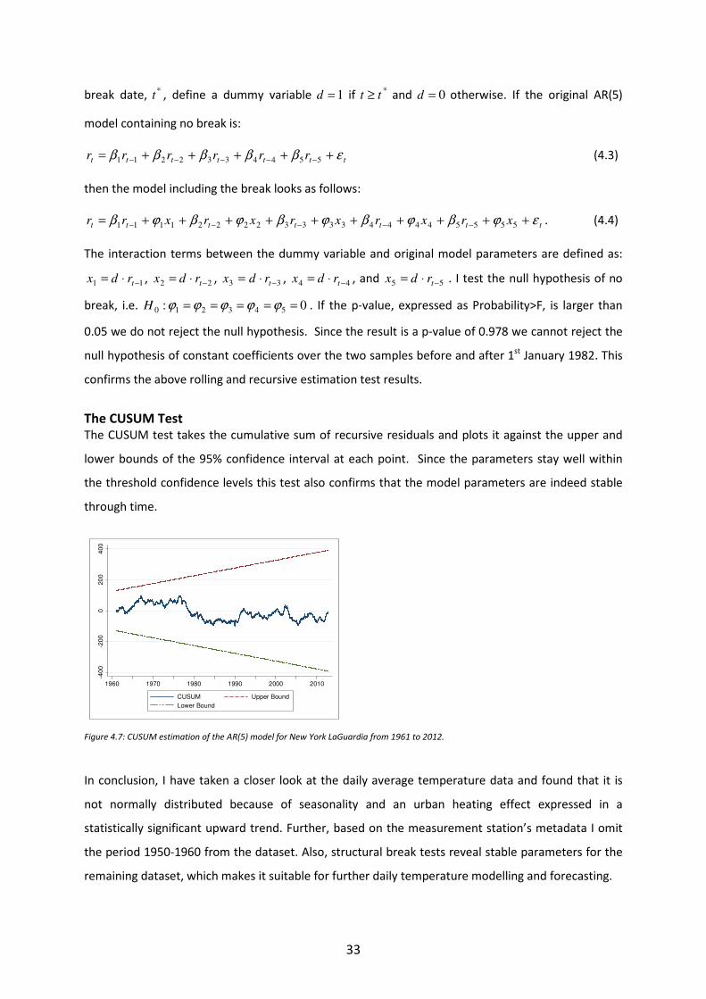
33

break date, *t , define a dummy variable 1=d if *

tt ≥ and 0=d otherwise. If the original AR(5)

model containing no break is:

ttttttt rrrrrr εβββββ +++++= −−−−− 5544332211 (4.3)

then the model including the break looks as follows:

ttttttt xrxrxrxrxrr εϕβϕβϕβϕβϕβ ++++++++++= −−−−− 55554444333322221111 . (4.4)

The interaction terms between the dummy variable and original model parameters are defined as:

11 −⋅= trdx , 22 −⋅= trdx , 33 −⋅= trdx , 44 −⋅= trdx , and 55 −⋅= trdx . I test the null hypothesis of no

break, i.e. 0: 543210 ===== ϕϕϕϕϕH . If the p-value, expressed as Probability>F, is larger than

0.05 we do not reject the null hypothesis. Since the result is a p-value of 0.978 we cannot reject the

null hypothesis of constant coefficients over the two samples before and after 1st January 1982. This

confirms the above rolling and recursive estimation test results.

The CUSUM Test

The CUSUM test takes the cumulative sum of recursive residuals and plots it against the upper and

lower bounds of the 95% confidence interval at each point. Since the parameters stay well within

the threshold confidence levels this test also confirms that the model parameters are indeed stable

through time.

-40

0-2

00

020

04

00

1960 1970 1980 1990 2000 2010

CUSUM Upper Bound

Lower Bound

Figure 4.7: CUSUM estimation of the AR(5) model for New York LaGuardia from 1961 to 2012.

In conclusion, I have taken a closer look at the daily average temperature data and found that it is

not normally distributed because of seasonality and an urban heating effect expressed in a

statistically significant upward trend. Further, based on the measurement station’s metadata I omit

the period 1950-1960 from the dataset. Also, structural break tests reveal stable parameters for the

remaining dataset, which makes it suitable for further daily temperature modelling and forecasting.

34

5. Temperature Modelling and Methodology

This chapter starts by explaining what elements a dynamic temperature model should contain.

Afterwards, I present the two main models and their submodels, and discuss some of the submodel

estimation results. In the next chapter daily average temperature forecasts and index forecasts are

performed from these dynamic temperature models.

5.1 The Modelling Framework As the data analysis in the previous chapter shows, daily average temperature is characterized by

seasonal cycles describing periodic temperature variations over the different seasons and a possible

upward trend due to urbanization and/or global warming. What is more, temperature values today

are dependent on previous’ days temperatures. Also, as observed by Alaton et al. (2002) and

Campbell and Diebold (2002), amongst others, the daily variance of temperature contains a seasonal

pattern. This means that temperature volatility changes with the seasons.

The aim of any good dynamic temperature model is to be sufficiently complex to describe all these

different components of temperature while at the same time be sufficiently simple to produce

accurate forecasts. The danger of having too complex a model, overfitted as it were, is that minor

fluctuations in the data can be exaggerated, thus leading to a poor forecast performance.

I choose to model the in-sample data using adaptations of the Campbell and Diebold (2005) model

and the expanded Benth-Šaltytė-Benth (2007) model, which is discussed in Benth-Šaltytė-Benth

(2012). Hereafter I will refer to these original main models as the CD and BSB model, respectively.

Whereas the authors only test their model on daily average temperature (DAT), I will run these

models on daily minimum and daily maximum temperatures as well. In doing so, I hope to capture

additional temperature characteristics specific to these extreme measurements, that would

otherwise be cancelled out. Further, keeping in mind the considerable length of the in-sample

dataset (1961-2010) I will test the models using 1) a simple linear time trend and 2) a quadratic time

trend. A quadratic time trend has, to the best of my knowledge, not been tested before on dynamic

temperature models for derivative pricing. Last but not least, Considine (1999) claims that any city

exhibiting a strong warming trend will be better approximated using the most recent ten years of

data. I put this statement to the test and also run the models on an in-sample dataset from 1st

January 2001 to 31st December 2010. This makes for a total of nineteen different models, which I

refer to as submodels:

35

Adaptations of CD Model Submodel 1 Submodel 2 Submodel 3a Submodel 3b Submodel 4a Submodel 4b Submodel 5 Submodel 6a Submodel 6b

In-sample period 1961-2010 x x x x x x

In-sample period 2001-2010 x x x

Modelled on DAT x x x

Modelled on daily max temperature x x x

Modelled on daily min temperature x x x

Linear Trend x x x

Quadratic Trend x x x

No Trend x x x

Adaptations of BSB Model Submodel 7 Submodel 8 Submodel 9a Submodel 9b Submodel 10a Submodel 10b Submodel 11 Submodel 12ab Submodel 12a Submodel 12b

In-sample period 1961-2010 x x x x x x

In-sample period 2001-2010 x x x x


Modelled on daily max temperature x x x

Modelled on daily min temperature x x x x

Linear Trend x x x x

Quadratic Trend x x x x x

No Trend x Table 5.1: The submodels and their underlying fundamental elements.

36

All original model and submodel estimation results are included in Appendix B. Due to space

constraints I will only insert graphs from the CD and BSB model for daily average temperature for the

period 1961-2010.

5.2 The Adapted Campbell and Diebold Model (2005) The first model I will test is a non-structural daily time series approach by Campbell and Diebold

(2005), which builds on their previous study from 2002. CD’s dataset consists of daily average air

temperatures (DAT) from four U.S. measurement stations for the period 1st January 1960 to 5th

November 2001: Atlanta, Chicago, Las Vegas, and Philadelphia. The in-sample dataset in this study

consists of daily air temperature measurements for New York LaGuardia from 1st January 1961 to 31st

December 2010. CD use a time series decomposition approach whereby a temperature series is

broken down into a number of characteristic temperature components, which are then properly

modelled in the hope of ending up with a pure random process, also known as random noise or

white noise. To model temperature seasonality the authors choose a Fourier approximation. They

also allow for a deterministic linear trend to account for warming effects in the temperature series. I

will allow for a quadratic trend as well. Other cyclical dynamics apart from seasonality are captured

by autoregressive lags, p, in an AR(p) process. The so-called CD conditional mean model looks as

follows:

=tT tTrend + tSeasonal + )( pAR + ttεσ (5.1)

where tT denotes the daily temperature and the different components are:

taaTrend t 10 += (5.2a)

or

2

10 taaTrend t += (5.2b)

where the linear term of the quadratic trend is omitted as it is not statistically significant for any

submodel.

=tSeasonal ∑=

+

G

g

gsgc

tdgb

tdgb

1

,,365

)(2sin

365

)(2cos ππ (5.3)

where gcb , and gsb , , Gg ,...,1= , are the respective parameters of the cosine and sine terms for

frequency order, G .

37

pt

P

p

pt TpAR −

=

−∑=1

)( α (5.4)

where pt−α , Pp ,...,1= , are the parameters of the AR(p) process

and

)1,0(~iid

tε . (5.5)

In equation (5.3) )(td is a repeating step function cycling through each day of the year. CD remove

February 29th from each leap year to obtain years of 365 days. In order to preserve complete use of

the in-sample dataset, however, I prefer not to adapt my data for leap years. Instead I follow Svec

and Stevenson’s (2007) approach by setting one cycle equal to 1461 days, i.e. four years:

=tSeasonal ∑=

+

G

g

gsgc

tdgb

tdgb

1

,,1461

)(2sin

1461

)(2cos ππ (5.6)

Following Campbell and Diebold (2002), and for illustrative purposes, I first regress the above model

(5.1) by ordinary least squares (OLS). All models - except the ten-year models - have a statistically

significant linear trend and quadratic trend with a p-value of 0.000. The linear and quadratic trend

results show that the daily average temperature at New York LaGuardia Airport has increased by

about 3.13˚F (1.7˚C) or 1.67˚F (0.9˚C), respectively, over the past fifty years. This reconfirms the

urban heat island effect which is present at the location. It is interesting to note that the quadratic

trend increases at a slower rate than the linear trend.

CD let the Akaike (AIC) and Bayesian Information Criteria (BIC) guide them in selecting which order to

use for the sine and cosine functions and temperature lags. These criteria indicate that using yearly,

half-yearly, and four-month frequencies (i.e. 3=G ), and setting 25=P is more than adequate for

all cities in their study. For the in-sample data at LaGuardia, I try out different Fourier orders ranging

from yearly, half-yearly, four-month, quarterly, and even 2.4 month frequencies. For each submodel I

let statistical significance at the 5% level determine the appropriate order of the frequencies. As it

turns out, using the first to first three of the mentioned frequencies provides a good fit to the 10-

year and 50-year submodels, with an average coefficient of determination of 89.95%. Furthermore,

CD allow for 25 lags as these help capture long-memory dynamics (autocorrelation) and in view of

the fact that their dataset contains a large number of degrees of freedom. Still, as Benth-Šaltytė-

Benth (2012) point out: “It is unclear if there is any meteorological explanation as to why today’s

temperature should explicitly depend on what happened 25 days ago” (p. 596). I therefore again look

at the statistical significance of the autoregressive parameters of each submodel individually. For the

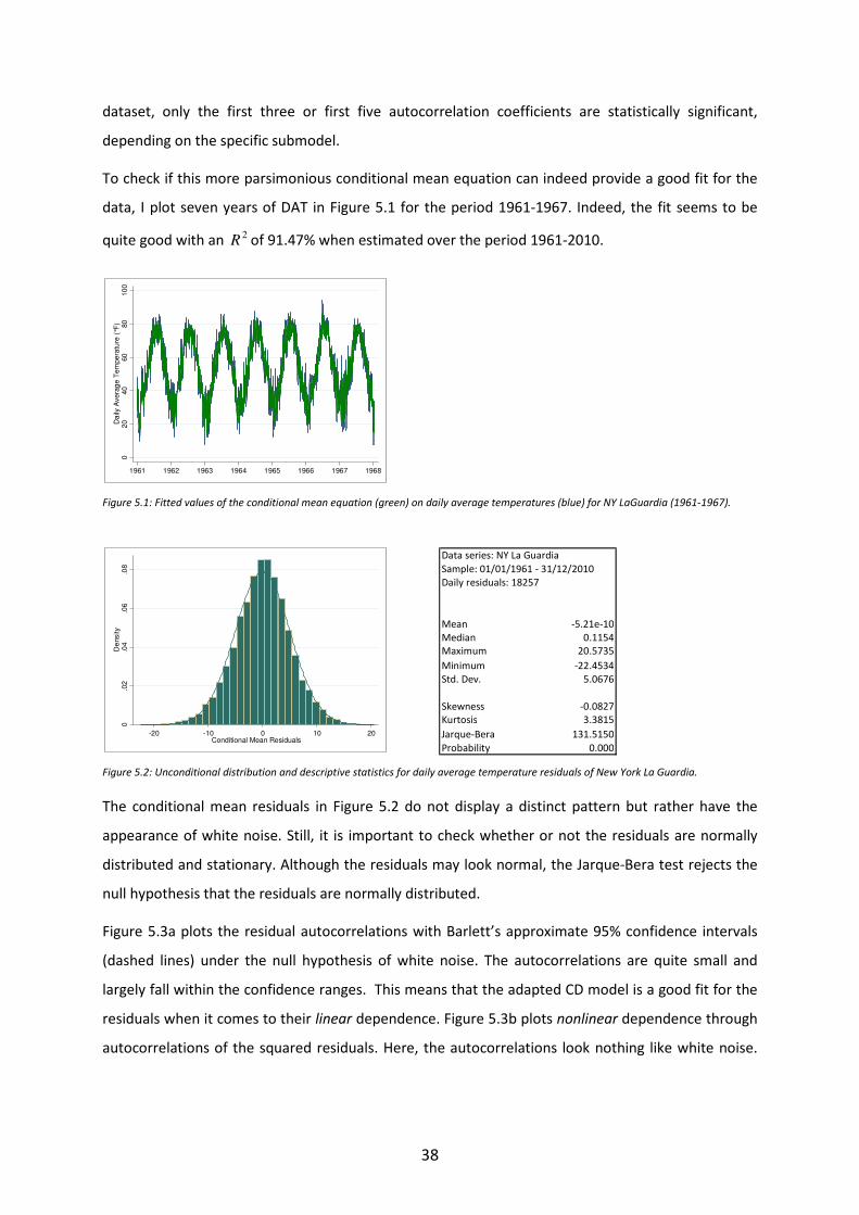
38

dataset, only the first three or first five autocorrelation coefficients are statistically significant,

depending on the specific submodel.

To check if this more parsimonious conditional mean equation can indeed provide a good fit for the

data, I plot seven years of DAT in Figure 5.1 for the period 1961-1967. Indeed, the fit seems to be

quite good with an 2R of 91.47% when estimated over the period 1961-2010.

02

04

060

80

10

0D

aily

Ave

rag

e T

em

pe

ratu

re (

°F)

1961 1962 1963 1964 1965 1966 1967 1968

Figure 5.1: Fitted values of the conditional mean equation (green) on daily average temperatures (blue) for NY LaGuardia (1961-1967).

0.0

2.0

4.0

6.0

8D

ensity

-20 -10 0 10 20Conditional Mean Residuals

Data series: NY La Guardia Sample: 01/01/1961 - 31/12/2010Daily residuals: 18257

Mean -5.21e-10Median 0.1154Maximum 20.5735

Minimum -22.4534Std. Dev. 5.0676

Skewness -0.0827Kurtosis 3.3815

Jarque-Bera 131.5150Probability 0.000

Figure 5.2: Unconditional distribution and descriptive statistics for daily average temperature residuals of New York La Guardia.

The conditional mean residuals in Figure 5.2 do not display a distinct pattern but rather have the

appearance of white noise. Still, it is important to check whether or not the residuals are normally

distributed and stationary. Although the residuals may look normal, the Jarque-Bera test rejects the

null hypothesis that the residuals are normally distributed.

Figure 5.3a plots the residual autocorrelations with Barlett’s approximate 95% confidence intervals

(dashed lines) under the null hypothesis of white noise. The autocorrelations are quite small and

largely fall within the confidence ranges. This means that the adapted CD model is a good fit for the

residuals when it comes to their linear dependence. Figure 5.3b plots nonlinear dependence through

autocorrelations of the squared residuals. Here, the autocorrelations look nothing like white noise.

39

On the contrary, they show evidence of seasonal persistence. Campbell and Diebold (2002) find this

particular type of dependence in seven out of ten U.S. cities they examined. -0

.20

-0.1

00.0

00.1

00.2

0A

CF

of r1

0 200 400 600 800Lag

Bartlett's formula for MA(q) 95% confidence bands

-0.2

0-0

.10

0.0

00

.10

0.2

0A

CF

of

r1sq

0 200 400 600 800Lag


Figures 5.3a & 5.3b: Correlogram of the residuals (Left) and squared residuals (Right) of the conditional mean for New York LaGuardia (800

lags).

To tackle the modelling problem, CD preserve the conditional mean model (5.1) and introduce an

additional model for the remaining variance in the model errors. Their so-called conditional variance

model not only takes into account seasonal volatility in the daily temperature but also other cyclical

volatility:

( ) 2

11

2

1

,,

2

1461

)(2sin

1461

)(2cos st

S

s

s

R

r

rtrtr

J

j

jsjct

tdjc

tdjc −

==

−−

=

∑∑∑ ++

+

= σβεσαππσ (5.7)

)1,0(~iid

tε (5.8)

In equation (5.7) seasonality is again modelled by a Fourier series. Apart from seasonal cycles, other

cyclical volatility is described by means of a Generalized Autoregressive Conditional

Heteroscedasticity process, i.e. GARCH process (Engle 1982; Bollerslev 1986, cited by Campbell and

Diebold, 2005), where R and S in equation (5.7) denote the order of ARCH and GARCH terms,

respectively. CD use the same number of waves as in the conditional mean equation, i.e. setting

3=J , and again apply AIC and BIC to determine the adequate GARCH model for their cities, i.e.

, 1=R , and 1=S . I rely on statistical significance and consider each submodel individually, resulting

in between one to four Fourier frequency terms. As for the GARCH model, I find that a GARCH(1,1) is

statistically significant for most models, except for the 10-year minimum temperatures where an

ARCH(1) model provides a better fit. For the other submodels, using a higher order GARCH model

would produce a negative coefficient, which undesirably can result in a negative value for the

conditional variance as well (Enders, 1995).

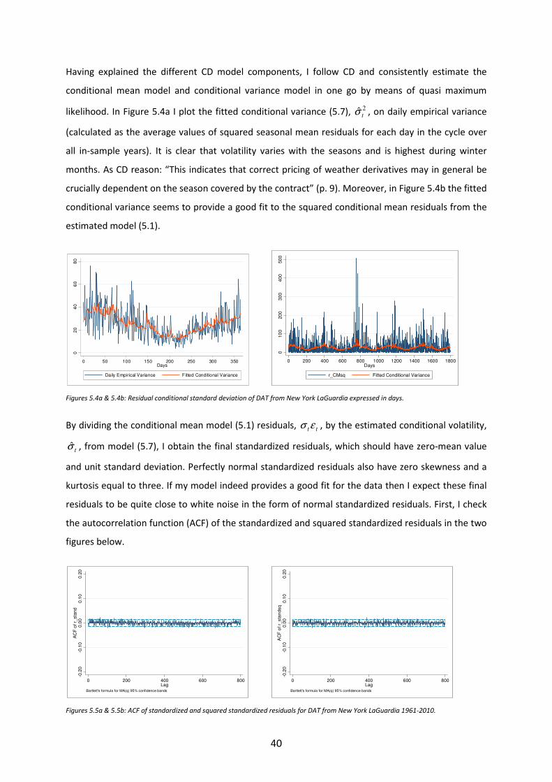
40

Having explained the different CD model components, I follow CD and consistently estimate the

conditional mean model and conditional variance model in one go by means of quasi maximum

likelihood. In Figure 5.4a I plot the fitted conditional variance (5.7), 2ˆtσ , on daily empirical variance

(calculated as the average values of squared seasonal mean residuals for each day in the cycle over

all in-sample years). It is clear that volatility varies with the seasons and is highest during winter

months. As CD reason: “This indicates that correct pricing of weather derivatives may in general be

crucially dependent on the season covered by the contract” (p. 9). Moreover, in Figure 5.4b the fitted

conditional variance seems to provide a good fit to the squared conditional mean residuals from the

estimated model (5.1).

02

04

06

08

0

0 50 100 150 200 250 300 350Days

Daily Empirical Variance Fitted Conditional Variance

010

020

030

040

050

0

0 200 400 600 800 1000 1200 1400 1600 1800Days

r_CMsq Fitted Conditional Variance

Figures 5.4a & 5.4b: Residual conditional standard deviation of DAT from New York LaGuardia expressed in days.

By dividing the conditional mean model (5.1) residuals, ttεσ , by the estimated conditional volatility,

tσ̂ , from model (5.7), I obtain the final standardized residuals, which should have zero-mean value

and unit standard deviation. Perfectly normal standardized residuals also have zero skewness and a

kurtosis equal to three. If my model indeed provides a good fit for the data then I expect these final

residuals to be quite close to white noise in the form of normal standardized residuals. First, I check

the autocorrelation function (ACF) of the standardized and squared standardized residuals in the two

figures below.

-0.2

0-0

.10

0.0

00

.10

0.2

0A

CF

of r_

sta

nd

0 200 400 600 800Lag


-0.2

0-0

.10

0.0

00

.10

0.2

0A

CF

of

r_sta

ndsq

0 200 400 600 800Lag


Figures 5.5a & 5.5b: ACF of standardized and squared standardized residuals for DAT from New York LaGuardia 1961-2010.

41

What is obvious is that there is no visual trace of seasonality in the variance that was present in

Figure 5.3b. The final residuals do indeed resemble white noise. Next, I plot the histogram and

quantiles of the standardized residuals against the quantiles of a normal distribution. The histogram

still displays some residual extra kurtosis and negative skewness. Indeed, the Jarque-Bera test for

normality shows an improved but not completely normal value of 38.45.

0.1

.2.3

.4D

ensity

-4 -2 0 2 4Standardized Residuals

Data series: NY La Guardia Sample: 01/01/1961 - 31/12/2010Daily standardized residuals: 18262

Mean 0.0069Median 0.0273Maximum 3.6091Minimum -4.1227Std. Dev. 1.0000


Figure 5.6: Unconditional distribution & descriptive statistics of standardized DAT residuals for New York LaGuardia 1961-2010.

-4-2

02

4S

tan

dard

ize

d R

esid

uals

-4 -2 0 2 4Inverse Normal

Figure 5.7: Qnorm plot of standardized daily average temperature residuals for New York LaGuardia 1961-2010.

These findings are supported by the qnorm plot, which presents a close, though not perfect, match

to a normal distribution. Normality values for the other CD submodels vary, generally producing

encouraging results. The final standardized residuals which closest resemble white noise are those of

the 10-year DAT and maximum temperature submodels. The worst performing submodels are the

two 50-year minimum temperatures submodels. This is due to remaining high kurtosis, which is

difficult to remove. On the whole, though, the fitted CD model adaptations look adequate enough for

forecasting purposes. In the following chapter I will therefore be performing out-of-sample

temperature forecasts on all CD submodels.

5.3 The Adapted Benth and Šaltytė-Benth Model (2012) Benth and Šaltytė-Benth (2012) present a discrete-time extension30 of the popular continuous-time

Ornstein-Uhlenbeck model in Benth and Šaltytė-Benth (2007). Like CD, BSB present a time series

42

decomposition approach whereby temperature is broken down into the same characteristic

elements of seasonality, time trend, autoregressive process, and seasonal variance component.

Their in-sample dataset consists of daily average air temperatures for Stockholm from 1st January

1961 to 31st December 2004. The main difference between the BSB model and the CD model is that

BSB propose a stepwise estimation approach, following Benth and Šaltytė-Benth (2007), Benth et al.

(2007) and Šaltytė-Benth, Benth, and Jalinskas (2007). This means that the different model

components are estimated one after the other instead of all at once, which is the case in the CD

model. BSB claim that by applying a step-by-step procedure and examining all intermediate residuals,

they manage to build a confident dynamic temperature model. They further state that by estimating

all the components together in one go, CD introduce uncertainty in the parameter estimates. The

BSB seasonal mean function is as follows:

ttttT εσµ += (5.9)

where tµ denotes the mean and tε represents the i.i.d. residual process. Here,

( )ptpt

P

p

ptt STS −−

=

−+= ∑1

αµ (5.10)

where as before, pα , Pp ,...,1= , are the parameters of the autoregressive process. tS is a

deterministic function which represents the long-term average of temperature towards which the

temperature mean reverts because of the autoregressive process. This so-called BSB seasonal mean

function of temperature is similar to CD equation (5.6) and is modelled as follows:

∑=

+

++=

G

g

gsgct

tdgb

tdgbtaaS

1

,,10365

)(2sin

365

)(2cos ππ (5.11)

As is the case in the CD model, BSB introduce a simple linear trend, make use of Fourier analysis to

model a smooth seasonality pattern, and remove all dates of 29th February from their sample. The

adapted BSB seasonal mean functions for a simple linear trend, quadratic trend, and four-year step

function are:

∑=

+

++=

G

g

gsgct

tdgb

tdgbtaaS

1

,,101461

)(2sin

1461

)(2cos ππ (5.12)

and

∑=

+

++=

G

g

gsgct

tdgb

tdgbtaaS

1

,,

2

101461

)(2sin

1461

)(2cos ππ (5.13)

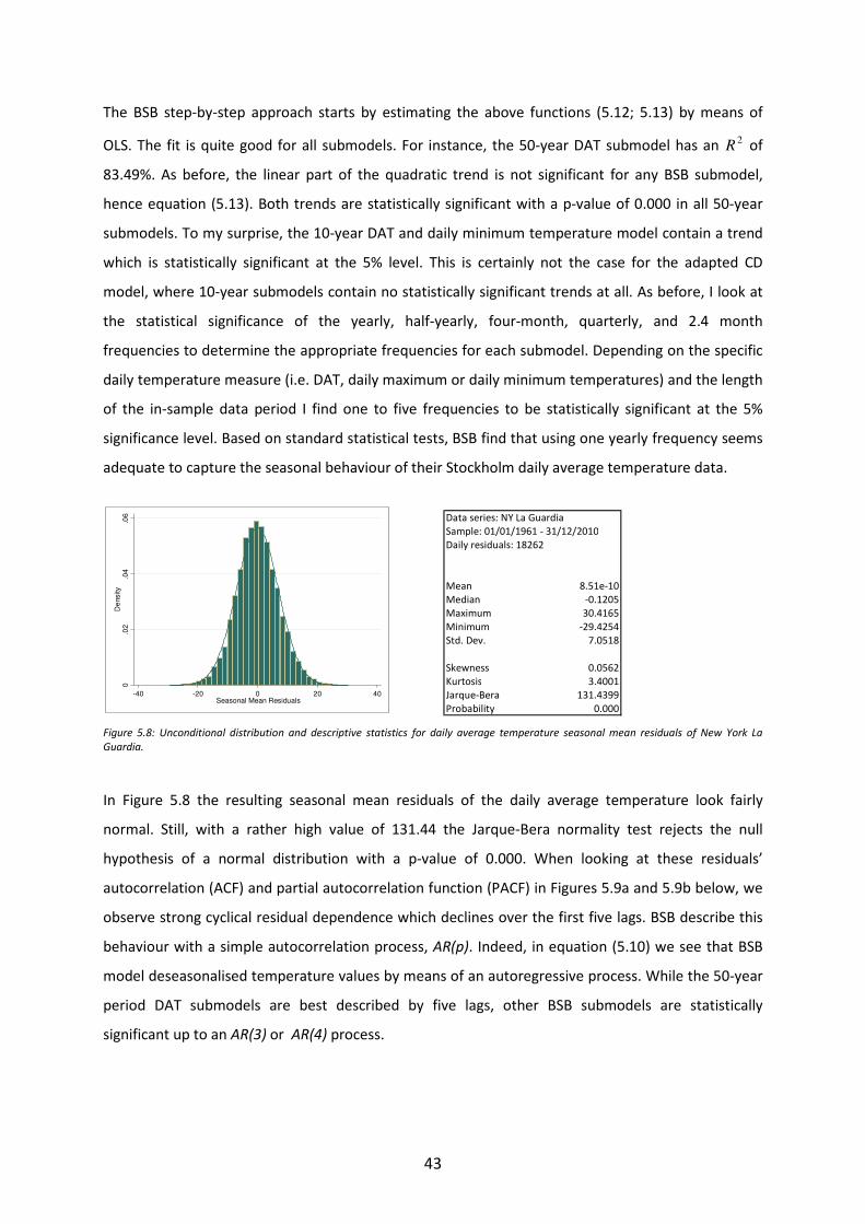
43

The BSB step-by-step approach starts by estimating the above functions (5.12; 5.13) by means of

OLS. The fit is quite good for all submodels. For instance, the 50-year DAT submodel has an 2R of

83.49%. As before, the linear part of the quadratic trend is not significant for any BSB submodel,

hence equation (5.13). Both trends are statistically significant with a p-value of 0.000 in all 50-year

submodels. To my surprise, the 10-year DAT and daily minimum temperature model contain a trend

which is statistically significant at the 5% level. This is certainly not the case for the adapted CD

model, where 10-year submodels contain no statistically significant trends at all. As before, I look at

the statistical significance of the yearly, half-yearly, four-month, quarterly, and 2.4 month

frequencies to determine the appropriate frequencies for each submodel. Depending on the specific

daily temperature measure (i.e. DAT, daily maximum or daily minimum temperatures) and the length

of the in-sample data period I find one to five frequencies to be statistically significant at the 5%

significance level. Based on standard statistical tests, BSB find that using one yearly frequency seems

adequate to capture the seasonal behaviour of their Stockholm daily average temperature data.

0.0

2.0

4.0

6D

ensity

-40 -20 0 20 40Seasonal Mean Residuals

Data series: NY La Guardia Sample: 01/01/1961 - 31/12/2010Daily residuals: 18262

Mean 8.51e-10Median -0.1205Maximum 30.4165Minimum -29.4254Std. Dev. 7.0518

Skewness 0.0562Kurtosis 3.4001Jarque-Bera 131.4399Probability 0.000

Figure 5.8: Unconditional distribution and descriptive statistics for daily average temperature seasonal mean residuals of New York La

Guardia.

In Figure 5.8 the resulting seasonal mean residuals of the daily average temperature look fairly

normal. Still, with a rather high value of 131.44 the Jarque-Bera normality test rejects the null

hypothesis of a normal distribution with a p-value of 0.000. When looking at these residuals’

autocorrelation (ACF) and partial autocorrelation function (PACF) in Figures 5.9a and 5.9b below, we

observe strong cyclical residual dependence which declines over the first five lags. BSB describe this

behaviour with a simple autocorrelation process, AR(p). Indeed, in equation (5.10) we see that BSB

model deseasonalised temperature values by means of an autoregressive process. While the 50-year

period DAT submodels are best described by five lags, other BSB submodels are statistically

significant up to an AR(3) or AR(4) process.

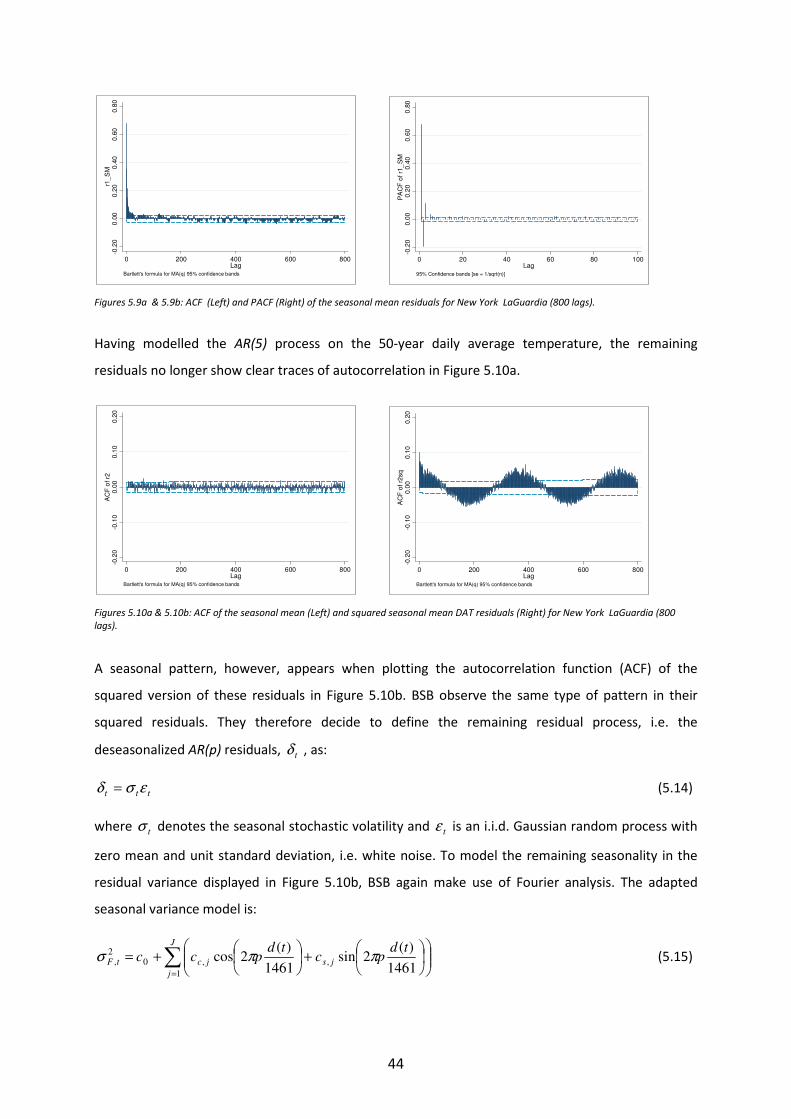
44

-0.2

00

.00

0.2

00

.40

0.6

00.8

0r1

_S

M

0 200 400 600 800Lag


-0.2

00.0

00.2

00

.40

0.6

00

.80

PA

CF

of

r1_

SM

0 20 40 60 80 100Lag

95% Confidence bands [se = 1/sqrt(n)]

Figures 5.9a & 5.9b: ACF (Left) and PACF (Right) of the seasonal mean residuals for New York LaGuardia (800 lags).

Having modelled the AR(5) process on the 50-year daily average temperature, the remaining

residuals no longer show clear traces of autocorrelation in Figure 5.10a.

-0.2

0-0

.10

0.0

00.1

00.2

0A

CF

of r2

0 200 400 600 800Lag


-0.2

0-0

.10

0.0

00

.10

0.2

0A

CF

of

r2sq

0 200 400 600 800Lag


Figures 5.10a & 5.10b: ACF of the seasonal mean (Left) and squared seasonal mean DAT residuals (Right) for New York LaGuardia (800

lags).

A seasonal pattern, however, appears when plotting the autocorrelation function (ACF) of the

squared version of these residuals in Figure 5.10b. BSB observe the same type of pattern in their

squared residuals. They therefore decide to define the remaining residual process, i.e. the

deseasonalized AR(p) residuals, tδ , as:

ttt εσδ = (5.14)

where tσ denotes the seasonal stochastic volatility and tε is an i.i.d. Gaussian random process with

zero mean and unit standard deviation, i.e. white noise. To model the remaining seasonality in the

residual variance displayed in Figure 5.10b, BSB again make use of Fourier analysis. The adapted

seasonal variance model is:

∑=

+

+=

J

j

jsjctF

tdpc

tdpcc

1

,,0

2

,1461

)(2sin

1461

)(2cos ππσ (5.15)

45

According to the estimation results of model (5.15), the 50-year DAT submodels only have one

statistically significant sine and cosine wave, while the other submodels require between one and

three such terms. All intercept parameters are statistically significant with a p-value of 0.000. In

order to assess the above model (5.15), I plot the fitted estimated variance, 2

,tFσ , against the

empirical variance of each day. Here, the empirical daily variances are calculated as before in the

adapted CD model.

02

04

06

08

0

0 50 100 150 200 250 300 350Days

Daily Empirical Variance Fitted Seasonal Variance

Figure 5.11: Time plot of the daily variances of final residuals and fitted seasonal variance for New York LaGuardia.

Just as observed in the adapted CD model, the variances are higher during the cold winter months

than during the warmer summer months. By dividing the final residual process, tε , by the fitted

estimated volatility, tF ,σ̂ , BSB filter out any residual seasonality. Indeed, we can see in Figures 5.12a

and 5.12b below that neither filtered nor squared filtered residuals (i.e. residual variances) display

any remaining seasonal pattern. On the other hand, the latter figure does show an unaccounted

GARCH-effect in the form of an upward brushing volatility peak over the first few lags.

-0.2

0-0

.10

0.0

00

.10

0.2

0A

CF

of r4

0 200 400 600 800Lag


-0.2

0-0

.10

0.0

00

.10

0.2

0A

CF

of

r4sq

0 200 400 600 800Lag


Figures 5.12a & 5.12b: ACF of the residuals (Left) and squared residuals after removing the seasonal variance.

To model the remaining GARCH effect BSB assume that for ttt εσδ = (5.14):

tGARCHtFt ,, σσσ ⋅= (5.16)

46

where

2

,2

2

11

2

, tGARCHttGARCH σβδβσ += − (5.17)

In short, BSB assume that the final model residuals can be explained by a product of a seasonal

deterministic function, a GARCH process, and an i.i.d. random Gaussian process, as follows:

ttt εσδ =

where tGARCHtFt ,, σσσ ⋅=

so that ttGARCHtFt εσσδ ⋅⋅= ,, (5.18)

BSB advocate the use of a multiplicative structure over CD’s additive structure because the former

solution avoids potential problems connected to the positive sign of the variance. Figure 5.13 plots

the squared deseasonalised residuals together with the fitted variance function 2

,

2

, tGARCHtF σσ ⋅ . For

the different submodels I find that a GARCH(1,1) or simple ARCH(1) model are statistically significant

and thus appropriate for my submodels.

010

02

00

30

04

00

50

0

0 200 400 600 800 1000 1200 1400 1600 1800Days

r2sq total_var = varBSB*varGARCH

Figure 5.13: Squared seasonal mean residuals & fitted variance function.

After removing the ARCH-GARCH effect I obtain the final standardized residuals. The autocorrelation

functions (ACF) of the standardized and squared standardized residuals are displayed below.

-0.2

0-0

.10

0.0

00

.10

0.2

0A

CF

of r5

0 200 400 600 800Lag


-0.2

0-0

.10

0.0

00

.10

0.2

0A

CF

of

r5sq

0 200 400 600 800Lag


Figures 5.14a & 5.14b: ACF of standardized and squared standardized residuals for DAT from New York LaGuardia 1961-2010.

47

All visual traces of ARCH-GARCH effects seem to have been filtered out successfully with the final

residuals resembling white noise. Finally, I plot the histogram and quantiles of the standardized

residuals against the quantiles of a normal distribution.

0.1

.2.3

.4D

en

sity

-4 -2 0 2 4Standardized Residuals

Data series: NY La Guardia Sample: 01/01/1961 - 31/12/2010Daily standardized residuals: 18262

Mean 0.0020Median 0.0240Maximum 3.6235Minimum -4.0352Std. Dev. 1.0000


Figure 5.15: Unconditional distribution and descriptive statistics of standardized daily average temperature residuals for New York

LaGuardia 1961-2010.

-4-2

02

4S

tan

da

rdiz

ed

Resid

uals

-4 -2 0 2 4Inverse Normal

Figure 5.16: Qnorm plot of standardized daily average temperature residuals for New York LaGuardia 1961-2010.

As is the case in the adapted CD model, the BSB histogram still shows some extra residual kurtosis

and negative skewness, while the qnorm plot reveals a pretty close match to a normal distribution.

With a value of 39.84 the Jarque-Bera test for normality performs only slightly worse than the 50-

year CD DAT model, which has a Jarque-Bera value of 38.45. As for the other BSB submodels, the

Jarque-Bera results are similar as those observed in the CD submodels. All in all, I decide that all BSB

model adaptations are sufficiently adequate to be included in next chapter’s out-of-sample

temperature forecasts.

48

6. Index Forecast Analysis

In this chapter, I explain how out-of-sample temperature forecasts are performed, and analyze the

index forecast results for the different submodels and a number of benchmark models by means of

the seven hypotheses formulated in Chapter 1.

6.1 Out-of-Sample Forecasting In the previous chapter I specified and estimated the in-sample parameters of the characteristic

components that form daily average temperature (DAT): trend, seasonality, autoregressive process,

and seasonal variance component. Putting these estimated elements together renders a simplified

version of the CD and BSB submodels:

tDAT = tttmean εσ+ (6.1)

where

)1,0(~iid

tε (6.2)

Dynamic one-step out-of-sample forecasts can now be performed. This means that as from the 1st

out-of-sample day, i.e. 1st January 2011, no realized daily average temperature values may enter the

forecasts. Rather, the first forecast, i.e. the temperature on 1st January 2011, is purely based on all

estimated in-sample parameters over the period 1961-2010. The second temperature forecast, i.e.

2nd January 2011, is produced from estimated in-sample parameters and the previous day’s forecast,

and so on. The result consists of 639 daily out-of-sample forecast values for the mean and seasonal

volatility, tσ , covering the period 1st January until 31st September 2012. The only element now

missing from equation (6.1) is the error term, tε . Given the fact that final errors are unknown I

simulate 1000 series of 639 daily Gaussian standardized errors. Using the same error series for all

submodels, 1000 series of 639 daily temperatures forecast values in the form of DAT, maximum

temperatures, or minimum temperatures can now be computed for each submodel. I also calculate

the arithmetic average of forecast maximum and minimum temperatures to obtain the DAT for the

specific CD and BSB submodels. This means that each series of maximum and minimum submodels

are merged into one submodel. The submodels after forecasting are thus as follows:

49

Adaptations of CD Model Submodel 1 Submodel 2 Submodel 3 Submodel 4 Submodel 5 Submodel 6


In-sample period 2001-2010 x x


The average of modelled daily max & min temperature x x x

Linear Trend x x

Quadratic Trend x x

No Trend x x

Adaptations of BSB Model Submodel 7 Submodel 8 Submodel 9 Submodel 10 Submodel 11 Submodel 12a Submodel 12b


In-sample period 2001-2010 x x x


The average of modelled daily max & min temperature x x x x

Linear Trend x x x

Quadratic Trend x x x x

No Trend Table 6.1: The submodels and their underlying fundamental elements.

50

The out-of-sample temperature forecasts for the 50-year linear CD and BSB submodels are displayed

in the graphs below.

20

30

40

50

60

70

80

90

100

Ja

n1

1

Fe

b11

Ma

r11

Apr1

1

Ma

y1

1

Ju

n11

Ju

l11

Au

g1

1

Se

p11

Oct1

1

No

v11

De

c11

Ja

n1

2

Fe

b12

Mar1

2

Ap

r12

May

12

Jun

12

Jul1

2

Aug

12

Se

p1

2

Oct1

2

Actual Temperature CD Submodel 1

Lower Forecast Limit Upper Forecast Limit

20

30

40

50

60

70

80

90

100

Ja

n1

1

Fe

b11

Ma

r11

Apr1

1

Ma

y1

1

Ju

n11

Ju

l11

Au

g1

1

Se

p11

Oct1

1

No

v11

De

c11

Ja

n1

2

Fe

b12

Mar1

2

Ap

r12

May

12

Jun

12

Jul1

2

Aug

12

Se

p1

2

Oct1

2

Actual Temperature BSB Submodel7

Lower Forecast Limit Upper Forecast Limit

Figure 6.1: Time plot of the forecast out-of-sample daily average temperatures with 95% prediction intervals for New York LaGuardia.

Next, I compute HDD or/and CDD indexes for each contract month during the out-of-sample period

using formulas (2.1) and (2.2) (see Chapter 2, p. 12), aggregating the resulting Degree Days over the

appropriate number of days per month. This produces 1000 simulated monthly indexes for each of

the 24 out-of-sample contracts months and per submodel. I retrieve the mean index forecast value

for each monthly contract and also the actual monthly index values from realized daily average

temperatures for the out-of-sample period. The index forecast results are summarized in Appendix C.

6.1.1 Comparing Index Forecast Accuracy

The mean index forecast performance of all models is compared to actual index values using

absolute errors (AE) and absolute percentage errors (APE):

AE = |actual index – forecast index|

APE = (AE/actual index)*100

In order to assess the different models’ mean forecast performance over time, I look at monthly

contracts and seasonal contracts. For the former, I select 2011 and 2012 contracts written on the

same HDD or CDD month and compute the contracts’ mean forecast errors. For instance, I take the

CDDApr11 and CDDApr12 contracts and look at how a CDD April contract performs for a given model,

averaging the two April contracts’ respective forecast errors. The following contract months are thus

included in the forecast analysis: HDDJan, HDDFeb, HDDMar, HDDApr, CDDApr, CDDMay, CDDJun,

CDDJul, CDDAug, and CDDSep.

Further, to broaden the scope of contracts that are included in the forecast analysis, I also look at

one winter and one summer contract. Seasonal contracts stretch over five months and are easily

obtained by aggregating the consecutive monthly index values. The HDD seasonal contract spans

51

from 1st November 2011 to 31st March 2012 while the CDD seasonal contract covers 1st May to 30th

September 2011. Mean forecast errors for mentioned monthly and seasonal contracts are displayed

in Appendix D.

6.1.2 Benchmark Models

Besides comparing the forecast index performance of the CD and BSB submodels vis-à-vis each other,

I also look at mean forecast performance relative to a number of benchmark models. These include

the two original main models, three naïve models, and the market model:

- The Original CD Main Model (2005) for in-sample period 1961-2001;

- The Original BSB Main Model (2012) for in-sample period 1961-2001;

- A 10-Year Average Index Model for in-sample period 2001-2010;



- The Market Model, using only market index forecasts dated 31st December 2010.

For the naïve average index models, monthly index values are computed for each in-sample year

after which the forecast monthly index values are calculated as the simple arithmetic average over

the entire in-sample period. Naturally, the market model is unknown as any highly successful index

forecast modelling strategies by traders are kept secret. All models contain daily temperature data

until 31st December 2010, after which forecasts are produced and compared over the next one to 21

months (i.e. until 30th September 2012).

6.2 Index Forecast Analysis In order to analyse the mentioned models’ forecast performance, I test all hypotheses formulated in

Chapter 1.

6.2.1 Hypothesis I

Hypothesis I states that:


LaGuardia daily temperature submodel based on a 10-year or 50-year dataset.


LaGuardia daily temperature submodel based on a 10-year or 50-year dataset.

52

To test hypothesis I, I compare the mean forecast performance of the following 50-year submodels

with their respective 10-year submodels (see Appendix D):

- Submodel 1 and Submodel 2 vs. Submodel 5; - Submodel 3 and Submodel 4. vs. Submodel 6;

- Submodel 8 vs. Submodel 11; - Submodel 9 vs. Submodel 12a;

- Submodel 10 vs. Submodel 12b.

Looking at Appendix D, 50-year submodels generally produce lower forecast errors than 10-year

submodels for HDD monthly contracts and the HDD seasonal contract. For CDD contracts, the 50-

year submodels produce lower forecast errors for all summer months except for June and

September. As for the summer seasonal contract, there is no difference in forecast performance for

the different length in datasets. In conclusion, we can reject the null hypothesis of there being no

difference in out-of-sample forecast performance between a New York LaGuardia daily temperature

submodel based on a 10-year or 50-year dataset.

6.2.2 Hypothesis II

Hypothesis II reads as follows:


LaGuardia daily temperature submodel using a simple linear or quadratic trend.


LaGuardia daily temperature submodel using a simple linear or quadratic trend.

Hypothesis II is tested by comparing the mean forecast performance of following linear trend

submodels vis-à-vis their respective quadratic trend submodels:

- Submodel 1 vs. Submodel 2; - Submodel 3 vs. Submodel 4;


- Submodel 12a vs. Submodel 12b.

As shown in Appendix D, the results are quite clear. All quadratic trend submodels outperform the

mean forecast performance of linear trend submodels for HDD contracts, both monthly and

seasonal. Moreover, quadratic trend models produce more accurate mean forecasts for all CDD

monthy contracts except for June. Still, all linear submodels outperform quadratic trend submodels

for the summer seasonal contract. Since quadratic trend submodels generally produce more accurate

forecasts than linear trend submodels, we can reject the null hypothesis of there being no difference

53

in index out-of-sample forecast performance between a New York LaGuardia daily temperature

submodel using a simple linear or quadratic trend.

6.2.3 Hypothesis III

Hypothesis III is formulated as follows:


LaGuardia daily temperature submodel based on forecast daily average temperatures and the

arithmetic average of forecast daily minimum and maximum temperatures.


LaGuardia daily temperature submodel based on forecast average daily temperatures and the

arithmetic average of forecast daily minimum and maximum temperatures.

Here, the following series of submodels are compared to their respective submodels:



- Submodel 8 vs. Submodel 10; - Submodel 11 vs. Submodel 12b.

The results are somewhat mixed for this hypothesis. While forecast DAT submodels perform better

than DAT submodels for HDD January contracts, this is not the case for HDD March and April

contracts. For all other contracts, no one series of submodels stand out. In short, we cannot reject

the null hypothesis of there being no difference in index out-of-sample forecast performance

between a New York LaGuardia daily temperature submodel based on forecast daily average

temperatures and the arithmetic average of forecast daily minimum and maximum temperatures.

6.2.4 Hypothesis IV

Hypothesis IV states that:

0H : There is no difference in index out-of-sample forecast performance between the two series of


1H : There is a difference in index out-of-sample forecast performance between the two series of


The following series of submodels are up for forecast error comparison:

54



- Submodel 5 vs. Submodel 11; - Submodel 6 vs. Submodel 12a and Submodel 12b.

The CD submodels outperform their corresponding BSB submodels for the HDD January contracts,

CDD June contracts, and the CDD seasonal contract. On the other hand, BSB submodels produce

lower forecast errors for three HDD months, four CDD months, and the HDD seasonal contract. In

short, the BSB submodels generally produce more accurate mean forecasts than their respective CD

submodels. Hence, we can reject the null hypothesis of there being no difference in index out-of-

sample forecast performance between the two series of corresponding New York LaGuardia

submodels.

6.2.5 Hypothesis V

Hypothesis V reads as follows:

0H : There is no difference in index out-of-sample forecast performance between the New York


1H : There is a difference in index out-of-sample forecast performance between the New York


Here I compare the following two series of models:

- Submodels 1 to 6 vs. the CD Original Main Model;

- Submodels 7 to 12b vs. the BSB Original Main Model.

First of all, original main models do not consistently outperform their respective submodels. Purely

taking into account the lowest forecast errors per contract, the CD original main model scores the

lowest value for four out of ten monthly contracts, whereas the BSB orginal main model only scores

better for one monthly contract. When looking at submodels with generally lower forecast errors,

there are five submodels that stand out. First of all, CD submodels 2 and 3 outperform the original

main CD model for seven contracts, including six monthly contracts and one seasonal contract.

Secondly, BSB submodels 8, 10, and 11 score lower forecast errors than their original main model for

no less than eight contracts, including seven monthly contracts and one seasonal contract.

Interestingly, all outperforming submodels are modelled with a quadratic trend, re-confirming

Hypothesis II. Given the above information, I reject the null hypothesis of there being no difference

55

in index out-of-sample forecast performance between the New York LaGuardia submodels and their

benchmark models.

6.2.6 Hypothesis VI

Hypothesis VI formulates that:

0H : There is no difference in index out-of-sample forecast performance between the two original


1H : There is a difference in index out-of-sample forecast performance between the two original


The two models whose mean index forecast performance is compared are:

- The CD Main Original Model vs. the BSB Main Original Model.

In general, there are very small forecast differences between the two original main models. Still, the

CD original main model and BSB original main model have a lower mean forecast error for three

contracts and six contracts, respectively. For the other contracts, the models produce near equal

results. Given the slightly improved forecast performance of the BSB original main model, I reject the

null hypothesis that there is no difference in index out-of-sample forecast performance between the

two original popular temperature models for New York LaGuardia.

6.2.7 Hypothesis VII

Finally, hypothesis VII states the following:

0H : There is no model that has an improved index out-of-sample forecast performance as compared


1H : There is a model that has an improved index out-of-sample forecast performance as compared


Here, all models are compared to each other, including all CD submodels, all BSB submodels, and all

benchmark models.

Whereas the three naïve average index models slightly underperform vis-à-vis all other models, the

market model generally outperforms all other models for HDD contracts. However, as is shown in

Appendix C, the market cannot give any accurate forecasts as from 19 months ahead in the future.

This is evidenced by the same monthly index number popping up between July-September 2012. As

for the CDD contracts, no one particular model stands out from the rest. On the other hand, the

56

forecast performance of all other models besides the market model seems less forecast horizon

dependent and more contract month dependent. This is in agreement with Svec and Stevenson

(2007), who find that the forecast length has little impact on the forecast accuracy of their testing

models. Oetomo and Stevenson (2005) also observe that the most appropriate model varies between

months, depending on the kind of model used. Given the market’s high performance for HDD

contracts, I reject the null hypothesis of there being no model that has an improved index out-of-

sample forecast performance as compared to all other models.

In conclusion, this analysis leads to a number of interesting findings:

1. The market model “knows best” between today and the next 19 months.

2. It is important for a trader to select the “best” model for his or her particular contract period.

3. Generally, though, quadratic trend models using 50-years of data provide the most accurate out-

of-sample forecast results.

4. Using a step-by-step modelling approach produces better out-of-sample forecast results than

modelling in one go.

5. Modelling on daily average temperature instead of forecast daily average temperature is

preferred. The results are no different and require less effort.

The fact that the market model generally provides better forecasts up till 19 months ahead in the

future means that the market possesses more accurate information than the one contained in the

other models discussed in the present study. In this connection, a couple of things are worth

mentioning. Though incorporating short-term weather forecasts and seasonal forecasts into future

index value expectations is no easy task, there are ways of doing so. Forecasts can, for instance, be

combined with daily temperature models or with models that model the HDD and CDD indexes

directly. This is especially useful for U.S. contracts where meteorological forecasts are available

around ten months before the start of the weather contract period (Jewson & Brix, 2007). Seasonal

forecasting in the U.S. mostly focuses on predicting possible El Niño and La Niña effects, i.e.

fluctuations in sea surface temperatures which cause warmer and colder winters than usual in New

York and the rest of the northern U.S., respectively. Besides making use of meteorological forecasts,

the market may be able to gather more accurate knowledge as to what kind of models and/or

combinations of models to use for specific contract periods.

57

7. Conclusion

This study aims at producing improved daily air temperature models to obtain more accurate index

values for New York LaGuardia airport. To achieve that goal two popular dynamic temperature

models were selected, from which a number of submodels were constructed and modelled. The

submodels comprised different combinations of dataset length, type of time trend, and type of daily

average temperature. The mean out-of-sample forecast performance of these submodels was

compared vis-à-vis each other but also by means of a number of submodels.

The author found that for the out-of-sample dataset for New York LaGuardia the market model

outperforms all other models up until 19 months ahead in the future. Further, it is imperative that a

trader select the right dynamic temperature model to match his/her New York LaGuardia contract

period. In the tough financial world even the smallest of forecast errors can cost dearly. For HDD

contracts, the obvious modelling choice is a 50-year quadratic trend model. For CDD contracts,

however, the choice is not so clear-cut. The study also observed that using the BSB step-by-step

modelling approach produces better out-of-sample forecast results than the CD in-one-go modelling

technique. And finally, modelling on daily average temperature instead of forecast daily average

temperature saves time and effort.

58

8. Further Research

Due to data and time constraints, the present study compares the performance of a number of

submodels for one location traded on the CME. However, given the relevance of choice of trend and

dataset length, it would be interesting to investigate if these two fundamentals also are important to

a larger number of other locations. Such other locations could, or could not, enjoy a similar

temperature climate as New York LaGuardia.

Moreover, weather derivatives also play a significant role in portfolio management. Given their

claimed low correlation to other assets, they can potentially reduce the risk in a mixed portfolio

considerably. A mixed portfolio could consist of bonds, equity, and weather derivatives. An

alternative would be to hold a pure weather portfolio with weather derivatives written on different

locations. And finally, the weather derivatives could be written on temperature or a mixture of

different weather parameters.

59

1 Lazo, Lawson, Larsen, and Waldman (2011, p. 712) define and measure weather sensitivity as “the variability

in gross product owing to weather variability, accounting for changes in technology and for changes in the level of economic inputs (i.e., capital, labour, and energy). This means that if weather-induced economic loss in one state A can be offset by changes in price or economic gain in state B, the impacts from an economic perspective will not be as apparent. 2 By traditional derivatives I am referring to derivatives written on equity, commodities, credit, interest rates,

or foreign exchange. 3 “Volume risk” or “quantity risk” is the risk that results from a change in demand from, or supply of, goods and

services due to a change in the weather, even if the prices remain unchanged (Brockett, Wang, & Yang, 2005). 4 An orange grower could, for instance, protect his or her business with a long call option for frost days and a

short futures contract for orange juice. This way he or she is covered against a higher number of frost days than expected which would adversely affect production, while at the same time hedging the crop’s sales price. 5 By assuming the role of buyer or seller in every exchange-traded sell or buy transaction, respectively, the CME

Clearing House ensures the integrity of each transaction, thereby eliminating any potential counterparty default risk. While standardized contracts entail basic risk, they are traded more frequently and are therefore often available at a more favourable price than OTC contracts. 6 It has, however, happened that someone with a long precipitation position attempts to seed the clouds

(Campbell & Diebold, 2002, p. 2)! 7 Information asymmetry deals with the study of decisions in a transaction where one party has more extensive

or more accurate information than the other (Mishkin & Eakins, 2003, p.24). 8 Moral hazard is present when an insured individual can increase his or her expected indemnity by actions

taken after having purchased insurance (Sharma & Vashishtha, 2007, p.115). 9 Note that energy companies trade as both hedgers on the demand side and as speculators on the supply side

of the weather derivatives market. 10

The Third Intergovermental Panel on Climate Change (IPCC) 2001 Report states that both simple extremes – such as higher maximum temperatures, more intense precipitation events – and complex extremes – such as intensified droughts and floods – are very likely or likely to occur in nearly all or many areas around the world for decades to come. Later IPCC reports support these 2001 findings.

11

Bellini (2005) does in fact allow for a linear and quadratic trend term in the mean temperature dynamics but finds no significant trend in her dataset. 12

The tick size is the monetary value attached to each minimum movement of the index value. 13

The names Heating and Cooling Degree Day originate from the U.S. energy sector. According to utilities, any deviation from the threshold temperature leads to higher energy demand as consumers either cool or heat their homes.

14

The CME rulebook lays down strict guidelines for the measurement times of the daily minimum and maximum temperature. For the New York LaGuardia weather station maximum and minimum temperatures are recorded between midnight and 11:59 p.m. 15

Arbitrage is the practice of making a riskless profit by taking advantage of mispricing in two or more securities or markets (Hull, 2006, p. 741).

60

16

Another characteristic of weather derivatives which precludes the use of the Black-Scholes-Merton model is the fact that weather options are Asian type options. This means that the underlying weather index at maturity is defined as a sum of values over the contract period instead of a single value (as in European or American options). 17

The expected payoff is discounted at the risk-free rate. This is generally the case in actuarial derivative pricing methods. This implies that the market price of risk is either ignored, assumed to be equal to zero, or is incorporated into the risk premium. 18

Brooks (2008, p. 208) explains that a series is strictly stationary if the distribution of its values remains the same as time progresses, implying that the probability that y falls within a particular interval is the same as at any time in the past or future. A weak stationary process should have a constant mean, a constant variance, and a constant autocovariance structure. 19

Moreno (2000) and Jewson and Brix (2007) argue that the above mentioned assumptions can be valid if burn analysis is applied on cleansed and detrended data. Still, their results indicate that even so the method produces inaccurate pricing results. 20

Considine (2005) looks at the validity of modelling the daily degree-day process (HDDs or CDDs) directly. She argues that the approach fails to describe an important part of the underlying temperature fluctuation because much information is discarded and lost due to the truncation point at the 65˚F threshold level. Moreover, zero degree-day values do not contain any useful information about the actual differences in threshold deviation. The same critique is valid for index modelling. 21

In a so-called ARMA(p,q) model p is the order of the autoregressive part and q is the order of the moving

average part. With tT denoting daily temperature, an ARMA(p,q) model can be represented as follows:

jt

q

j

jt

p

i

itit uuTT −

==

− ∑∑ ++=11

θφ

22 Suppose we are interested in finding the adjusted mean for April 2009. Let us say that the mean of the

average daily temperatures for the months of April is 60˚F (equation 3.2). Following equation (3.3) the observed monthly average for the year 2009 is 5˚F colder than average, namely 55˚F. If our daily averages

(equation 3.1) for April 1st

and April 2nd

are 58˚F and 63˚F, respectively, the mean adjusted averages, tyrT ,ˆ , are:

April 1st

: 58˚F + (55˚F - 60˚F) = 53˚F April 2

nd: 63˚F + (55˚F - 60˚F) = 58˚F

23

February 29th

is removed from each leap year in the dataset. 24

In mathematics, a stochastic Brownian motion is described by the so-called Wiener process. 25

An Ornstein-Uhlenbeck process is a stochastic process with asymptotic mean-reversion. Moreover, it has the attractive conditions of being stationary, Gaussian, and Markov (Doob, 1942). Because of its mean-reversion characteristic, the Ornstein-Uhlenbeck process is widely used in finance to model interest rates and commodity prices. The discrete-time analogue of an Ornstein-Uhlenbeck process is represented by an AR(1) model, i.e. a first-order autoregressive model. 26

WBAN stands for Weather-Bureau-Army-Navy. The National Climate Data Center (NCDC)’s homepage states that: “WBAN numbers were the first major attempt at a coordinated station numbering scheme among several weather reporting authorities. Original participants in the WBAN number plans were the United States Weather Bureau, Air Force, Navy, and Army, and the Canadian Department of Transportation”. 27

MacDonald Dettwiler and Associates (MDA) is an international firm specialized in geographic information technologies. For more information, visit: http://www.mdaus.com/

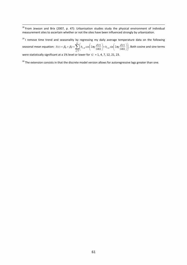
61

28

From Jewson and Brix (2007, p. 47): Urbanisation studies study the physical environment of individual measurement sites to ascertain whether or not the sites have been influenced strongly by urbanization. 29

I remove time trend and seasonality by regressing my daily average temperature data on the following

seasonal mean equation: ∑=

+

++=

G

g

gsgc

tdgb

tdgbttS

1

,,101461

)(2sin

1461

)(2cos)( ππββ . Both cosine and sine terms

were statistically significant at a 1% level or lower for G = 1, 4, 7, 12, 21, 23.

30

The extension consists in that the discrete model version allows for autoregressive lags greater than one.

daily temperature modelling for weather derivative pricing€¦ · daily temperature modelling for...

Documents