Hysteresis in Market Response:

When is marketing spending an investment ?

Dominique M. Hanssens

and

Ming Ouyang

Revised, March 6, 2001

Dominique M. Hanssens is the Bud Knapp Professor of Marketing at the AndersonGraduate School of Management at UCLA. His e-mail address isdominique.hanssens@anderson.ucla.edu. Ming Ouyang is Assistant Professor at the CityUniversity of Hong Kong. His e-mail address is mkouyang@cityu.edu.hk. The authorsgratefully acknowledge the comments of Professors Bart Bronnenberg, Marnik Dekimpe,Aimee Drolet, Jin Zhang and Dongsheng Zhou on drafts of this paper.

Hysteresis in Market Response:

When is marketing spending an investment ?

Abstract

Conventional wisdom says that it takes ever increasing marketing budgets and/or

lower prices to create sustained growth in sales, which may or may not be profitable in

the long run. However, some documented cases and conceptual evidence suggest that

marketing spending or prices can exhibit hysteresis in market response, a condition where

temporary changes in the marketing mix are associated with permanent movements in

sales performance. As such, hysteresis creates a long-run investment benefit from

marketing actions, which can be highly beneficial to the firm, or detrimental to

competition. Yet the assessment and formal implications of market response hysteresis

for marketing resource allocation are unexplored.

This paper addresses the modeling of marketing hysteresis in three ways: one, it

shows how the presence of full vs. partial hysteresis in response may be assessed from

longitudinal data on sales and marketing-mix allocations. Two, it develops the link

between sales hysteresis and profit hysteresis, and derives the long-run optimal spending

rules for a firm whose marketing efforts exhibit some form of hysteresis. Three, it

illustrates both the measurement of hysteretic marketing effects and their optimal

spending implications for a leading supplier of computer printers. The paper concludes

with an agenda for future research in this important, yet under-researched area of

marketing strategy.

Keywords: marketing mix, long-term marketing effects, marketing resource allocation,

econometric models, time-series analysis

1

Introduction

Motivated by the financial expectations of their private or public stakeholders,

businesses continuously search for new ways to achieve profitable growth. The marketing

component of this search is focused on reaching higher plateaus of sales and market share

that are preferably sustainable. However, these higher levels are not necessarily more

profitable, as the sales response function is typically characterized by decreasing returns

to scale. In such cases, higher sales or market share inevitably require sustained higher

marketing spending, which may or may not be profitable in the long run.

A far more attractive scenario to the marketer is when only temporary marketing

efforts are needed to achieve sustained sales growth, a condition sometimes called

hysteresis. Hysteresis is the tendency of a stimulus-induced response to stay at a higher

level even after the stimulus is removed. The concept was first used in the nineteenth

century in the physical sciences and has since been used to explain economic phenomena

such as unemployment and trade deficits. In marketing, Little (1979) first suggested that

sales response to advertising could exhibit hysteresis. An overview of the use of the

hysteresis concept in various scientific disciplines in shown in Table 1.

Marketing-induced sales hysteresis creates two ways in which marketing

spending can foster sales growth over time: one is the triggering function, i.e. the

temporary - if costly - investment that brings about a new, higher sales plateau and, two,

the maintenance function, or the sustained spending that preserves the higher sales. All

else equal, the stronger the marketing hysteresis, the more budget can be allocated to

short-term triggering (investing) and the less to sustained maintenance, which creates

more profitable long-run economics. Under full hysteresis, marketing is pure investment,

which triggers an increase in market performance that is sustainable without subsequent

marketing spending. Without hysteresis, sustained sales growth needs to be nurtured by

permanently higher marketing spending, so that marketing loses its one-time investment

character. Figure 1 illustrates the difference between full hysteresis and partial hysteresis

in marketing.

2

______________________________

Table 1 – History of Hysteresis

_______________________________

______________________________

Figure 1 – Full and Partial Marketing Hysteresis

_______________________________

While hysteresis is not a common part of the managerial or even academic

marketing vocabulary, its existence is implied by several well-known marketing

phenomena. For example, when a financial services provider engages in an effective

customer acquisition campaign, the incremental revenue stream that is perpetually

generated by loyal new customers points to a hysteretic effect of that campaign.

Similarly, when new-product trial is followed by repeat purchasing or when new-product

adoption by an innovator leads to positive word-of-mouth and adoption by imitators, any

role that marketing plays in temporarily stimulating the trial or adoption may have a

hysteretic sales effect over time. Hysteresis is also at the core of the current US

government allegation that, in the mid-nineties, American Airlines competed unfairly in

certain regional markets in which new low-cost entrants were trying to establish a

foothold. For example, according to the New York Times (May 14, 1999), prior to

competitive entry in the Dallas – Colorado Springs route, American flew an average of

3,723 monthly passengers between these cities, at an average fare of $158. When low-

cost competition entered, American reacted with a combination of more flights and lower

prices. This resulted in 19,909 monthly passengers on the route, at an average fare of $88,

which drove the new entrants out of the market. Finally, American allegedly

reestablished its higher price point, an average of $133 in this case, but was now able to

draw 9, 237 monthly passengers on average. Taking these numbers at face value, we

would conclude that American’s temporary marketing activity resulted in a permanent

gain of over 5,500 passengers per month, with incremental monthly revenue exceeding

$600,000.

3

Causes and Implications of Marketing Hysteresis

Why would marketing-induced consumer response stay at a higher level even

after the stimulus is removed ? When a marketing stimulus such as an ad campaign or a

sales visit is effective, it changes consumer attitudes, for example by creating an

awareness or preference for the advertised product. We expect such changes to be self-

sustaining because, once a consumer is made familiar with an offering, he or she cannot

easily be made unfamiliar with it. Attitudes and/or attitude components may be stored in

long-term memory to be retrieved for later use, rather than reconstructed on every

occasion (Fishbein & Ajzen 1975). Consequently, at the level of attitudinal response, we

expect effective marketing efforts to be hysteretic, i.e. temporary stimuli can have

sustained response.

However, attitudinal change in and of itself may be insufficient to justify a

marketing investment. Only under certain conditions (e.g. an attitude is sufficiently

strong) will changes in attitude result in changes in behavior (e.g. purchase behavior) that

are economically beneficial to the marketer. Once engaged, such behavioral changes can

become self-sustaining, even independent of attitudes, if it is advantageous to the

consumer to do so. For example, marketing-induced product trial may lead to user

satisfaction, which in turn creates habit-forming repeat purchase behavior, because the

satisfied consumer saves time and effort in exploring other alternatives. However, new

market conditions may emerge (for example competitive activity) that interfere with the

self-sustained behavior and diminish or even remove the hysteretic effect. The more

intense that interference, the more the marketer has to engage in maintenance marketing

spending in order to protect the hysteretic effect, which is of course costly. In the limit,

there is no hysteresis at all, and any desired sustained sales growth will require

permanently higher spending. Thus a priori we expect the hysteresis in marketing-

induced behavior change to be partial at best, and we will need a metric that represents a

range from zero to partial to full hysteresis. Marketing conditions that favor hysteresis

include newer product categories with growing demand, product and marketing

4

differentiation, price flexibility and high consumer switching costs. Conditions that

disfavor hysteresis are price wars and other forms of intensive competitive reaction,

undifferentiated products and marketing, stable demand patterns and low consumer

switching costs.

For the marketer, the first critical task in engaging hysteresis is to obtain initial

consumer response (attitudinal or behavioral), i.e. there should be short-run marketing

effectiveness. Now, it is well known that most sales-to-marketing elasticities are below

unity, and some are quite small on average (e.g. advertising elasticities average .1 to .2).

Other short-run marketing elasticities are higher, but it takes a substantial and sustained

effort to execute such marketing initiatives, as in the case of sales force and distribution.

Both of these observations suggest that hysteresis is probably not the rule in market

response. In fact, Simon (1997) argued that single marketing actions may not be potent

enough to create a hysteretic effect on sales. However, the combination of timely

marketing effort and advantageous circumstances – both of which are temporary – can

trigger a stronger immediate behavioral change (a higher response elasticity) which is

more likely to be hysteretic. From a customer perspective, such temporary circumstances

include marketing incentives such as a price cut, an invitation to join a loyalty program,

or a chance to acquire a limited-supply product. They also include environmental

conditions that make the marketing activity unusually salient. For example, Simon (1997)

illustrates that the consumption of the Gorbatschow-brand vodka in Germany rose

fivefold after Mikhael Gorbachev rose to power in the (then) Soviet Union. When the

brand’s environmental conditions later returned to normal (i.e. the Gorbachev regime

ended in 1991), the behavioral change in their vodka sales was self-sustaining,

presumably because the target market had become habitual Gorbatschow consumers and

saw no reason to switch brands. In conclusion, the combination of a favorable external

situation, along with innovative company action across several marketing-mix

instruments, is more likely to result in hysteresis.

The antithesis of hysteresis is mean-reverting sales response to marketing, which

can be zero-order or distributed over time (carryover effects). Zero-order (current) effects

have been reported in several cases involving price response, whereas distributed-lag

effects are more typically associated with advertising response (see Hanssens, Parsons &

5

Schultz 2001). In either case, even though marketing is effective in that there is a non-

zero response elasticity, once the marketing stimulus is removed, the behavioral change

dissipates, either immediately or gradually, and sales adopt a stationary (e.g. mean-

reverting) pattern over time. In such cases, achieving sustained growth in market

performance will require either permanently lower prices and/or permanently higher

marketing spending .

The study of marketing hysteresis therefore raises new modeling opportunities

and challenges, both empirical and analytical. From an empirical perspective, we must

establish evolution (permanent change) in market performance, and we must relate that

evolution to temporary changes in marketing support, possibly mitigated by external

circumstances. We must also develop a metric that quantifies the hysteretic effects on a

continuous scale. From an analytical perspective, we must set up the marketing resource

allocation problem as a long-run optimization in which trigger actions may well have

permanent effects on performance, with or without the need for follow-up (maintentance)

actions. These are the objectives of our research.

We begin with a brief discussion of existing market-response models and how

they are ill equipped to capture hysteresis. That motivates the design of an

implementable modeling approach for hysteresis: we formulate empirical conditions on

longitudinal marketing data, and we develop a metric that gauges the strength of

hysteresis on a 0-to-1 scale, i.e. ranging from zero to partial to full hysteresis. Next, we

study dynamic resource allocation under hysteresis, in particular the question of how

much to spend on triggering vs. maintenance, where the former is upfront, temporary

marketing investment and the latter is sustained spending. We then combine

measurement and optimization in an actual case study of a leading supplier of a high-

technology product. We econometrically estimate and validate the relative strength of

hysteresis in marketing campaigns for this durable product in its evolving market. We

also derive marketing investment prescriptions that exploit hysteresis to create a

substantial gain in long-term profitability. The paper ends with a number of

recommendations for future research in this new area.

6

Market Response Models and Hysteresis

The majority of market-response models are of the ‘level-level’ form, where a

certain level of spending is associated with an equilibrium level of performance, possibly

after some temporal adjustment (see, e.g. Hanssens, Parsons and Schultz 2001).

Therefore, optimization rules lead to spending prescriptions that are increasing in sales,

i.e. the higher the desired result, the higher the required spending. Among those, the best

known rule, due to Dorfman and Steiner (1954), states that the short-run profit

maximizing monopolist optimally spends on advertising (for example) as follows :

ADVERTISING ε ADV

_______________ = ________

REVENUE | ε PRICE |

where ε refers to elasticity. The rule implies that, with certain price and advertising

elasticities (for example, -2.5 and 0.1, respectively) there exists an optimal advertising-to-

revenue ratio, in casu 4 %. Numerous extensions of the Dorfman-Steiner conditions

exist, for example those accommodating long-term profit maximization (e.g.

Schmalensee 1972), competitive reactions (e.g. Lambin, Naert and Bultez 1975) and

goodwill accumulation and depletion (e.g. Vidale and Wolfe 1957, Nerlove and Arrow

1962). These extensions, however, do not change the basic premise that marketing

resources should be allocated in proportion to their response elasticities, and that higher

sales performance always requires higher spending levels.

Some market response models incorporate the possibility that optimal spending

allocations are uneven over time. Specifically, the literature on pulsing and chattering –

mostly in the context of advertising – has demonstrated conditions under which it is

optimal to pulse:

• with an S-shaped response curve, pulsing may allow the manager to allocate a

restricted budget in the concave portion of the curve, whereas even spending may

result in perennial advertising below the threshold response level (in the convex

portion of the curve) (e.g. Sasieni 1971, 1989),

7

• even with a concave response curve, the presence of advertising wearout justifies a

pulsing strategy, as it helps avoid the loss of advertising effectiveness due to

excessive repetition (e.g. Naik, Mantrala and Sawyer 1998).

The resulting dynamic allocation rules are more complex, allowing, for example,

for substantial frontloading of spending, followed by longer periods of lower-level

efforts. Similarly, in a diffusion-of-innovation framework, conditions exist that lead to

aggressive optimal marketing spending early in the product life cycle (e.g. Horsky and

Simon 1983). This aggressive early spending shifts the sales pattern forward, though total

lifetime sales remain the same. Despite their temporal complexity, these models still have

the property that marketing effects on sales are temporary and therefore, higher

equilibrium sales require higher marketing spending.

Hysteresis changes this basic premise, because there is no longer a one-to-one

mapping of marketing effort into sales performance. Instead, temporary spending

deviations from any level could result in permanent increases in sales. Therefore, in order

to capture hysteresis in response, (1) some specific temporal sales and marketing

behaviors should be observed, and (2) the response model itself should include the effect

on sales of a change in marketing from any existing level of spending. Formally, the

hysteresis conditions on the data and the response model are:

• sales (or the relevant market response measure) should change over time, and

that change should be of a permanent nature. Indeed, in the opposite case of

stationary sales behavior, all sales fluctuations are temporary and the sales

level eventually reverts back to the mean (or a deterministic trend) ;

• the hysteretic marketing action should be temporary. By contrast, if the

marketing action is permanent, then it represents sustained spending which,

however effective, always implies higher spending for higher results ;

• sales evolution should be linked to the temporary marketing action. Without

that link, there is of course no market-response effect, even though the

temporal conditions on the data are met.

Assessing these conditions can be done by using modern time-series techniques and

incorporating the results in the specification of a market-response model. For example, a

8

unit-root test on sales should reveal evolution or I(1) behavior, and the same test on the

marketing variable should reveal stationarity or I(0) behavior (see e.g. Hanssens, Parsons

and Schultz 2001 for details on such tests). An empirical generalizations study has

revealed that about two thirds of sales time series, one third of market- share time series,

and half of marketing-mix variables are evolving (Dekimpe and Hanssens 1995b).

Therefore, a priori the univariate conditions for marketing hysteresis exist on a

substantial subset of marketing data. These conditions are summarized in the ‘hysteresis’

cell of Dekimpe and Hanssens’ four strategic marketing scenarios described in Figure 2

(Dekimpe and Hanssens 1999).

_____________________________________________

Figure 2 – Evolution and Stationarity in Marketing Effort

and Market Performance

_____________________________________________

Given evolving sales and stationary marketing, a hysteresis response model would

establish a significant relationship between changes in sales and temporary marketing

activity. Such a result was recently discovered on marketing scanner data: temporary

price promotions for a private-label brand of soup were found to have a long-run market-

expansive effect on the category (Dekimpe, Hanssens and Silva-Risso 1999).

In many cases, though, the observed sales evolution is caused by factors other

than marketing hysteresis. Among them, there could be evolution in the external

environment, e.g. rising disposable personal incomes, or evolution in the marketing mix

such as steadily higher distribution (e.g. Bronnenberg et al. 2000). Such co-evolution can

also be assessed by time-series methods, in casu the presence of cointegration between

sales and other evolving variables (external or marketing) (see, e.g. Powers, Hanssens,

Hser and Anglin 1991; Franses 1994). We therefore need to construct a metric for

hysteresis that can distinguish the hysteretic effects of marketing from the long-term

effects of evolution in the environment or in the marketing mix. Furthermore, if the

hysteresis is partial, a mixture of temporary and sustained marketing efforts should enter

into the response function. Temporary efforts (changes) trigger higher sales, but

9

subsequent maintenance efforts (levels) are needed to preserve the sales gains. Partial

hysteresis is not an explicit scenario in Figure 2. Instead, it combines the two sales-

evolving scenarios in the figure, and motivates our development of a new hysteresis

metric.

A Hysteresis Metric

A hystereris metric, ρ, should accommodate a mixture of evolvingi and stationary

time series, along with the possibility that actual hysteresis is absent, partial or full. For

that purpose we postulate a general class of market-response functions that are log-linear

to accommodate nonlinear returnsii. We shall first describe the hysteresis response model

and later address the temporal properties of the data. Let

S = sales,

A = log marketing spending of any kind,

Z = other sales drivers, which may or may not have hysteretic effects,

then marketing hysteresis ρ is derived from the following response function

S (t) = c + φ S (t-1) + α [A(t) - ρ A(t-1) ] + θ Z (t) + u(t), (1)

where u(t) is an error term with the standard assumptions, and effective marketing

implies α > 0 (see e.g. Gordon (1989) for a similar specification in macro-economics).

This model is made empirically tractable by rearranging terms as:

S (t) = c + φ S (t-1) + α [ ( 1 - ρ ) A(t) + ρ ∆ A(t) ] + θ Z (t) + u(t) (2)

where ∆ is the difference operator, i.e. ∆ A(t) = A(t) - A(t-1). Therefore, in the estimation

equation

S (t) = c + φ S (t-1) + b1 A(t) + b2 ∆ A(t) + θ Z (t) + u(t) (3)

and the degree or strength of hysteresis ρ is estimated from

10

ρ = b2 / ( b1 + b2 ),

so hysteresis is conveniently measured as the magnitude of the change effect relative to

the total (level + change) effect. Absent hysteresis (ρ ≤ 0), only the levels of marketing

affect sales. Under ρ=0, equation (1) reduces to the conventional current-effects response

model in levels

S (t) = c + φ S (t-1) + α A(t) + θ Z (t) + u(t) (4)

and under ρ<0, it becomes a distributed-lag effects model in levels:iii

S (t) = c + φ S (t-1) + α A(t) + β A(t-1) + θ Z (t) + u(t) (5)

where β = - α ρ. Conversely, full hysteresis (ρ=1) implies that sales are driven only by

changes in marketing spending, regardless of levels:

S (t) = c + φ S (t-1) + α [A(t) - A(t-1) ] + θ Z (t) + u(t). (6)

Finally, partial hysteresis is obtained when both levels and changes of marketing impact

sales, i.e. 0<ρ<1. This metric is not only empirically tractable, it also provides an

intuitive definition of marketing hysteresis: marketing is decomposed as level plus

change, and hysteresis is the relative importance of marketing change in driving sales

evolution.

Can hysteresis be detected in combination with temporary response effects ?

More complex distributed-lag versions of (1) and (3) can be specified if there was

reason to believe that “change in marketing spending” involved more than one period (as

in the case of advertising wear-in), and/or if market response consists of hysteresis with

carryover effects. A more general version of our hysteresis estimation equation (3)

accommodates this as follows:

S (t) = c + φ S (t-1) + b1 (L) A(t) + b2 (L) ∆ A(t) + θ Z (t) + u(t) (7)

11

where L is the lag operator and the bi (L) (i=1,2) are lag polynomials representing

temporary, delayed response effects of marketing on sales, i.e. bi (L) = b0i + b1i L +

b2i L2 + … In that case the hysteresis metric would be estimated as

ρ = b2 (1) / [ b1 (1) + b2 (1) ]

The generalized form (7) does not change the substance of hysteresis measurement and

its resource implications. We will only use it in empirical application and determine the

shapes of the distributed-lag functions bi (L) (i=1,2) by direct-lag search.

In conclusion, a hysteresis metric can be developed starting from conventional

market-response models, by imposing specific conditions on the dynamic response

parameters. This approach offers the advantage that current and decaying marketing -

effects models are nested in the hysteresis model. For the empirical detection of

hysteresis we must first turn to the temporal properties of the variables.

Temporal Behavior

Model (1) and its estimation version are sufficiently general to accommodate

various temporal behaviors in marketing and sales, each with their own unique set of

conditions on the parameters. First, and foremost, sales must be evolving, i.e. its time

series has a unit root. Given that S(t) is I(1):

• under full hysteresis, only temporary changes in marketing spending have an impact.

There is no long-term relationship between sales and marketing levels, i.e. no

cointegration between their time series. The conditions on the parameters are φ=1,

ρ=1 and α>0. This is the “hysteresis” cell in Figure 2. Its strategic implication is that

only trigger or temporary investment spending is needed to permanently increase

sales. An example is a customer acquisition campaign that yields new and loyal

accounts without the need for subsequent customer retention spending.

• absence of hysteresis, ρ ≤ 0. In this case, there may be a long-term marketing effect

in levels, i.e. α>0 and 0<φ<1, the “co-evolution” cell in Figure 2 which necessitates

ever higher marketing spending for higher sales goals. An example is increasing

spending on brand advertising in order to obtain higher distribution levels which, in

12

turn, enable higher sales results. It is also possible that sales evolution is altogether

unrelated to marketing spending, i.e. α=0 and φ=1.

• partial hysteresis involves right-hand-side terms in (1) that are all contributing to sales

growth, i.e. 0<φ<1, 0<ρ<1 and α>0. A “trigger” marketing campaign (temporary

spending hike) lifts sales to a higher plateau, and a subsequent adjustment in

maintenance spending prevents mean reversion in sales, i.e. a return to lower levels.

Both triggering and maintenance are necessary: without trigger, there is no sales lift

to a higher level, and without maintenance, that higher level is not sustainable. Cast in

terms of Figure 2, this scenario combines the lower-left and lower-right quadrants:

evolving marketing levels (“maintenance”) plus temporary marketing changes

(“triggering”) drive the evolution of sales performance. This combined

trigger/maintenance effect of marketing breaks the one-to-one relationship between

marketing spending and sales performance. An example is successful customer

acquisition spending followed by sustained retention spending in order to prevent

attrition of the newly acquired customers.

Equation (3), estimated with ordinary least squares, produces consistent estimates

of the parameters (φ b1 b2 θ ), even though sales are I(1). This is because there exist

values for the coefficients for which the error term is I(0) (see e.g. Hamilton 1994,

Chapter 18). Equation (3) is preferred over a specification in the changes of sales,

because the latter would remove potentially useful information contained in the levels of

marketing, in particular the marketing maintenance function. As an alternative, we could

specify a vector-error correction response model (e.g. Powers et al. 1991), which

combines changes and levels, however such a model requires the cointegration condition

between marketing and sales to hold, which we do not want to impose on the data a

priori.

Hysteresis of Marketing Campaigns

The response model (1) accounts for hysteretic effects of both increases and cuts

in marketing spending. In our context, however, it is more appropriate to work with an

asymmetric form of (1) that isolates the hysteretic effects of marketing investments or

13

campaigns, which are identified as temporary increases in marketing spending. Indeed,

managers generally aim at growth in financial performance, for which they are willing to

engage in certain marketing actions, as in the American Airlines example in the

introduction. Hysteresis in marketing campaigns is also consistent with the theoretical

considerations we discussed earlier. For example, the attitude-storage theory of Fishbein

and Ajzen (1975) may be used to hypothesize a hysteretic effect of positive changes in

marketing (in casu, advertising) spending only. Under this hypothesis, the advent of an

advertising campaign causes sales to evolve to a higher level. When the campaign ends,

sales do not return to their pre-campaign levels. Instead, they fluctuate at a different level,

depending on the amount of maintenance spending and the strength of hysteresis.

Model (1) and its estimation version (3), are easily adapted to measure the

hysteresis of marketing campaigns by restricting changes in spending to positive values:

S (t) = b0 + φ S (t-1) + b1 A (t) + b2 max [A(t) - A(t-1)] , 0

+ θ Z (t) + u (t) (8)

Note that a similar specification was used in the Adpuls model (Simon 1982),

except of course that sales are not mean reverting in our case. The strength of hysteresis

is once again measured by the quantity b2 / ( b1 + b2 ).

Can there be hysteresis in marketing spending cuts ? Many marketers are

understandably concerned about reducing marketing support, lest it permanently damages

the brand’s market performance. If the spending cuts are sustained, their sales impact will

be measured by the level term and its parameter b1 in equation (8). Beyond the level-

impact, if we want to test the hypothesis that even a temporary reduction in support has a

permanently damaging effect on sales, we could augment equation (8) with a temporary

spending cut variable defined, for example, as min [A(t) - A(t-1)] , 0 . We are not

aware of any a priori reasons for hypothesizing such an effect, though.

14

Difference with impulse-response modeling.

Our hysteresis metric, ρ, is not the only way in which hysteresis can be assessed

empirically. Dekimpe and Hanssens (1995a, 1999) have used a vector-autoregressive

(VAR) time-series model for this purpose, in which the impulse-response function of any

pair of variables (X,Y) is used to detect hysteresis, defined as the permanent effect on Y

of a one-unit (or one standard-deviation) shock in X. That approach produces a numerical

and a visual path of impulse-response weights that can be used in a simulation of long-

term sales and profit consequences of certain marketing actions (see Dekimpe and

Hanssens 1999). However, as reduced-form parameters the impulse-response weights

cannot be used directly in a dynamic optimization framework, nor can they accommodate

partial hysteresis.

By contrast, the present approach combines level (maintenance) and difference

(trigger) effects of marketing on sales in a single-equation model that lends itself to

optimal resource allocation over time in evolving markets, with either zero, full or partial

hysteresis. Marketing spending is therefore a control or exogenous variable, whereas in

the VAR modeling approach, there are no a priori exogenous variables. The two metrics

use the same initial stage of testing for evolution vs. stationarity in the data, and they

complement each other in addressing different hysteresis modeling objectives. The VAR

model offers a complete description of a dynamic multi-equation marketing system, (i.e.

without exogeneity), whereas the hysteresis response model addresses the long-run

optimal allocation of a marketing resource under control of the firm (i.e. with

exogeneity).

Optimal Triggering and Maintenance Spending

Optimal marketing resource allocation is affected by hysteresis because economic

returns may be captured quickly and permanently. Ceteris paribus, we expect higher

hysteresis to imply more frontloading of marketing investments and less maintenance

spending. The economic dynamics of this intuitive result are complex, as they involve

both response and economic parameters in an evolving environment. We will use the

15

well-established principles of unit-root detection and modeling in time series to

characterize such evolving environments (e.g. Dekimpe and Hanssens 1995).

The key to hysteresis estimation is the term [A(t) - ρ A(t-1)] in Equation (1). The

value of ρ indicates how a "change in A" , i.e. a temporary marketing action, generates

permanent (non-decaying) effects on sales. An optimization model with hysteresis

should, therefore, capture the spirit of the expression [A(t) - ρ A(t-1)].

Dynamic problem formulation

Let

S(t): sales or demand for a product at time t, a positive function of goodwill;

g: goodwill, a positive function of current and previous marketing, similar to the

specification in Nerlove and Arrow (1962);

A (t): marketing spending in general;

AT(t): marketing investment for triggering the hysteresis effect;

AM(t): marketing spending for maintaining the triggered hysteresis effect. Absent

hysteresis, this spending is the same as general marketing spending;

P: price of the product;

C: unit variable cost of the product;

r: capital cost (discount rate);

M(A(t)): marketing cost function;

B(t): budget constraint.

Marketing resource allocation is motivated by long-run profitability. Therefore,

we use A(t) as a control variable and g as a state variable to maximize the firm's profit

stream Π from periods t=0 to t=T:

( )[ ]

( ).))1(),(()(

)9(,))(()(1

1maxmax

0)(

−=

−−

+Σ=Π ∑

=

tAtAgftSwith

tAMtSCPr

T

t

t

tA

16

The first line of Equation (9) is the standard formulation for choosing a marketing

spending policy A(t) to maximize a discounted profit stream Π over a planning horizon

(0, …, T) (e.g. Welam 1982). The second line of Equation (9) characterizes hysteresis

through a goodwill specification in the tradition of Nerlove-Arrow (1962). They treat

marketing (in casu, advertising) as an investment in the firm's goodwill which, in turn,

affects sales (Liu and Forker 1990). The general Nerlove-Arrow model is expressed as

S(t) = f(g(A(t)), but our goodwill specification is g(A(t), A(t-1)), which captures hysteresis

as explained in the previous sectioniv. It is therefore a more abstract expression of the

term [A(t) - ρ A(t-1)] in Equation (1). Furthermore, marketing budgets are consumed

between current trigger and future maintenance spending, so:

( ) )10()1()( tBtAtA MT ≤++

Equations (9) and (10) form our resource allocation problem. The dynamic optimization

is designed around a budget cycle with two sub-periods, one for triggering and one for

maintenance. This setting distinguishes our hysteresis modeling from conventional

marketing optimization studies. Indeed, the common nature of optimal policies in the

literature - including even spending, pulsing, chattering and their combinations - is that

they all recommend repetitive marketing actions (as summarized by Naik et al. 1998). In

contrast, we expect the optimal policy derived from this modeling to be non-repetitive, so

long as our strict hysteresis conditions are met.

The system in (9) and (10) can be simplified and made into a dynamic

programming problem over a discrete time horizon. Let:

parameter π = P-C stand for contribution margin,

time preference (1+r)-1 = β (β > 0 ),

goodwill be a Cobb-Douglas functionv: g = Aξ (t ) A -µ (t-1),

sales be a log function of goodwill: S(t) = ln g = ξ ln A(t) - µ ln A(t-1),

17

which allows for the assessment of zero, partial or full hysteresis as in the

previous section. It is important to note that our hysteresis metric ρ

developed from (1) equals µ / ξ in this sales response function,vi

the marketing cost function M(A(t) = ln A δ (t) = δ ln A(t). The cost

function alows for nonlinearities, for example due to quantity discounts in

media buying.

Substitute the above in Equation (9), then scale the parameters to unity by setting

π ξ - δ = 1, and let ( π µ ) / (π ξ - δ) = π µ = γ.

After rearranging items, our objective function becomes:

[ ] )11()1(ln)(lnmax

0)( ∑

=

−+ΣT

t

t

tAtAtA γβ

This objective function corresponds to the hysteresis response function (1)vii, and the

analytical hysteresis parameter γ is related to the empirical hysteresis coefficient ρ in

equation (1), as we demonstrate below. Note also that we make abstraction of separable

exogenous demand drivers other than marketing spending, such as product quality and

prices, so our results will be conditional on their levels.

Profit hysteresis (γ)

The new parameter γ can be interpreted as “profit weighted” hysteresis, as it

combines response hysteresis and profitability. Indeed, substituting ρ = µ / ξ in the

definition of γ reveals that γ = (π / (π - δ/ξ)) ρ. Now, δ/ξ is a measure of marginal

marketing cost, i.e. marginal cost of effort divided by responsiveness. The higher the

marketing cost, either because the effort is expensive (δ is high) or its response is low (ξ

is small), the more important the impact of response hysteresis on profit, i.e. ρ is

amplified. Likewise, when contribution margin is higher, profit hysteresis is increased.

On the other hand, when marketing is free (e.g. unpaid media publicity), δ=0 and

18

response and profit hysteresis are the same. As one would expect, zero response

hysteresis ρ or zero contribution margin π always imply zero profit hysteresis γ.

The marketing budget, B, is a given amount of money for marketing spending at

time t. The marketing manager could invest the entire budget immediately, or could

allocate only a portion for current spending and reserve another portion for future use.

Absent hysteresis, there would be no trigger spending, and the budget would be allocated

as in the extant literature, represented asviii: B(t) = AM(t). The constraint now becomes:

)12(),()()1()( tAtBtAtA MMT =≤++

This budget says that a lump-sum available resource, AM(t), will be allocated into two

parts: trigger (investment) spending AT(t) for the current period and maintenance

spending AM(t+1) for the future. Equations (11) and (12) form a dynamic system which

can be solved by Bellman's equation.

Analytical Solution

Chow (1997) shows that the rationale of dynamic programming is that the value

of the objective function at the end of the planning horizon is maximized first, and then

this maximized value is used as a constraint to determine the value of the present choice

variable. In our model, we first ensure that the (higher) sales plateau will last to the end

of T, no matter how long it is, and then we determine the current triggering action.

With given initial conditions: AM(0)>0 and AT(-1) known (for example, let AT(-1)

= 0), a recursive method can be used to find solutions for this system. The state for this

problem is the pair AM(t), AT(t-1), with the transition equation for the first element

given by the budget constraint, whereas the transition equation for the second element is

a simple function of the control AT(t). Then the Bellman equation for this system isix:

( ) MMT

TMTT

AA

TM

AAAts

AAvAAAAvMT

≤+

+−+=−

)'(..

)13(,),)'(()1(lnlnmax)1(,,

βγ

19

where AT = AT(t), and (AM)' = AM(t+1). From the structure of the Bellman equation, we

conjecture that the value function should be a form ofx:

v(AM, AT(-1)) = Φ + ΩlnAM + ΨlnAT(-1)

To verify this conjecture we must find a triplet (Φ,Ω,Ψ) such that the corresponding

value function satisfies Bellman's equation, that is:

MMT

TMTT

AA

TM

AAAts

AAAA

AA

MT

≤+

Ψ+Ω+Φ+−+

=−Ψ+Ω+Φ

)'(..

)14(,ln)'ln()1(lnlnmax

)1(lnln

)'(,βββγ

After the constraint has been imposed at equality, the first-order condition of the

maximization problem on the right-hand side yields xi:

)15(1

TMTTT AAAAA −Ω=Ψ++ ββγ

This gives us:

)16(1

1)( * BAT

γββγβ+Ω+Ψ+

+Ψ+=

and:

)17(1

)'( * BAM

γβββ

+Ω+Ψ+Ω=

where B is the budget. The triplet (Φ,Ω,Ψ) can be identified by substituting Equation (11)

back to Equation (10), and they can be expressed in terms of parameters (β, γ) xii. The

optimal solutions for partial profit hysteresis are given as:

20

Under full profit hysteresis (γ = 1) a corner solution exists where all marketing effort is

triggeringxiii, i.e. A T *= B.

This set of solutions for the firm's long-run profit maximization enables us to

allocate a given budget B into triggering and maintaining. The optimal policy is non-

repetitive, i.e. there is no need to trigger again once a firm arrives in the maintenance

stage, and this scenario is unique to hysteresis. Compared to conventional spending rules,

the optimal policy with hysteresis requires a smaller marketing budget for a given sales

target, or it could generate and maintain higher sales and profits for a given marketing

budget. The two-period model adequately characterizes the non-repetitive spending

nature, but does does not imply that the planning horizon must consist of two equal-

length periods. Instead, these two periods characterize two regimes, which may have

different lengths. In practice, the maintenance period will likely be significantly longer

than the triggering period.

Specifically, the results imply the following:

(i) Equations (18) and (19) show how to split a given budget into current triggering

and subsequent maintenance, which depends on the strength of hysteresis, γ. For a

given budget B, the greater the triggering, the smaller the maintenance spending,

and vice versa; under full profit hysteresis, all spending is triggering, and no

maintenance is required;

(ii) ∂AT/∂γ > 0, or the stronger the profit hysteresis, the greater portion of B should be

allocated to triggering. Note that higher profit hysteresis can be obtained either by

higher response hysteresis, or by higher profitability;

(iii) ∂AT/∂r > 0, or the greater the discount rate, the more budget dollars should be

allocated to current trigger spending ;

( )

)19(.)()(

)18(1;11

1)(

**

*

TM

T

ABA

BA

−=

−≠−

+

+= γβγ

βγ

21

Triggering Without Constraint

We can also use the solution to address the managerially important question of

resource allocation with given sales targets. Given the hysteresis response function (11),

for a given target level of sales S*, the necessary triggering amount of marketing is xiv:

In interpreting the important economic ramifications of Equation (20), recall that

triggering is upfront, temporary marketing spending, and that maintenance is permanent,

recurring spending. Hysteresis allows for a portion of the required maintenance spending

to be substituted by triggering, so that substantial marketing cost savings emerge in the

long run. The “penalty” for these savings is that the required trigger spending will be

higher, as all the hysteresis terms in Equation (20) are positive. Specifically, the

determinants of trigger spending are:

(i) the target itself (St* ). Ceteris paribus, the higher the target, the higher the

spending. Furthermore, absent profit hysteresis (γ = 0), this target level is the only

determinant of marketing spending. In that case, however, the spending has to be

sustained in every subsequent period, i.e. it becomes permanent maintenance

spending.

(ii) the profit-weighted strength of hysteresis (γ). We have already established that

stronger response hysteresis (ρ) justifies higher trigger spending. Furthermore, the

higher the profitability ( π / (δ/ξ - π) ) generated from response hysteresis, the

more can be allocated to temporary trigger spending as well.

(iii) the historical sales path, up to the most recent sales level (St-1 ). If, for example,

historical sales and hysteresis are high, more can be spent on triggering, resulting

in fewer required maintenance dollars in the future. Note also that, the longer the

time horizon (e.g. the older the product), the smaller the upfront penalty for

trigger spending. Indeed, in the limit (t→∞), optimal triggering approaches the

)20()(ln)(exp1

10

**

−Σ+−+= ∑−

=−

t

iit

itt

Tt

SASA γγ

22

asymptote of permanent spending. This is the lowest marketing-cost solution in

that an infinite spending stream has been fully replaced by a one-time investment

of the same amount. To the best of our knowledge, this is the first analytical

evidence that the evolution of historical sales itself can drive optimal long-run

marketing spending policies.

(iv) the inaugural marketing spending level (A0). Ceteris paribus, if initial sales for a

product were generated with little or no marketing support, that reduces the

required trigger spending penalty toward future sales targets, and vice versa. The

influence of this term, too, dies out as time progresses. This connection between

initial marketing conditions and future spending is also a new insight in the theory

of marketing resource allocation.

The general behavior of the optimal triggering expression (20) is illustrated in Figure 3,

where optimal trigger spending toward a given sales target varies with the strength of

profit hysteresis and inaugural marketing spending. Exogenous drivers of demand

naturally affect optimal triggering in (20) as well, via the sales terms in the exponent.

______________________________

Figure 3 – Drivers of Trigger Spending

_______________________________

Optimal Marketing Budgeting in Practice

The above analysis is based on a theoretical logical order, i.e., starting with an

objective function and a constraint, we derive a solution to this system. The practice of

marketing strategy, however, often proceeds in a reverse order. First, a marketing

campaign is designed in order to achieve a given target sales level, and the marketing

support budget is negotiated with senior management. However, the optimal marketing

budgets for a given target are rarely assessed in practice. If they were, then our solution

could be used in the following orderxv:

23

Step 1. Optimal triggering: for a given target sales, S*, Equation (20) can be used

to determine the optimal triggering, AT* = AT(S*);

Step 2. Optimal budgeting: use Equation (18) to determine the optimal budget, B*

= B(AT*);

Step 3. Optimal maintaining: use Equation (19) to split the optimal budget: AM*

= B* - AT*.

As a result, AT*, AM*, and B* can be expressed in terms of S* and parameters.

The remaining task in the paper is to demonstrate the use of our hysteresis metric

in an actual case setting, leading to a diagnosis of the company’s existing spending

patterns relative to long-term optimal.

The Hysteresis of Value Adjusted Advertising: A Case Study

The empirical detection of hysteresis

Hysteresis can be measured empirically either by direct or indirect sales-response

methods. If marketing is of a direct-response nature, longitudinal records of marketing

campaigns, customer acquisition and customer retention could be used to measure the

lifetime value of a customer and derive the spending policy that maximizes this quantity

(see, e.g. Blattberg & Deighton 1996). In this case, the more hysteretic sales response,

the more would be allocated to customer acquisition (triggering) at the expense of

customer retention (maintenance) efforts, and vice versa. This approach is relatively

simple to execute so long as the acquisition and retention-response parameters are stable

over time. On the other hand, its application is restricted to direct-response marketing and

it may overestimate marketing productivity, as each customer acquisition is fully

attributed to marketing action, which could have been redundant. For these reasons we

will not explore direct-response models in this context.

24

Indirect sales-response methods do not require a separate long-term metric of

market performance, as we isolate the permanent (long-term) component in sales

performance itself. As argued earlier, this method is anchored in the rich econometric

market-response literature and requires equal-interval data on sales and the marketing

mix for several years. The data interval should be response- and decision relevant, most

likely weekly to monthly in the context of marketing campaigns and budget allocations.

There is no restriction on the types of marketing activities that could generate hysteresis,

though our example will focus on the quantitative (spending) dimension of marketing,

consistent with the dynamic optimization model. Thus we require substantial detail on the

evolution of prices, period-by-period spending levels and results. Future research should

investigate whether or not qualitative changes in the marketing mix have hysteretic

effects on sales, as well as possible segment differences in hysteretic market response.

Data description

Our empirical application is set in the evolving market for computer printers in

the early to mid-nineties. This market development was spurred by the growing installed

base of personal computers, along with the advent of newer printing technologies such as

laser and inkjet. We sample monthly sales of a leading supplier of printers from 1990 to

1994, along with its marketing mix comprised of retail price, print and electronic

advertising spending, and a one-time expansion in distribution from specialty-only to

specialty plus general outlets (Figure 4).

A large-scale conjoint measurement was executed near the end of the time period,

so we have estimates of end users’ utilities for product features. This offers a unique

opportunity to quantify the relative attractiveness of the product relative to competition in

this fast-moving technology market. Indeed, by retroactively changing the product and its

competitors' attributes to coincide with actual historical market changes (such as an

improvement in print resolution from 300 to 600 dpi, or a reduction in product weight or

footprint), we can generate a time series of consumer utilities for the product. Figure 5

shows the history of these conjoint-inferred consumer preferences for the product. From a

customer value perspective, the product goes through phases of higher and lower values,

relative to its price and competitive offerings. We expect these relative-quality variations

25

to have a positive effect on consumer sales, while controlling for the other elements in the

marketing mix. Following the attitude and behavioral change framework discussed

earlier, we also expect communications efforts that coincide with periods of higher

product value to have a stronger effect on product sales.

______________________________

Figure 4 – Sales and Marketing Spending

_______________________________

____________________________

Figure 5 – Price and Consumer Inferred Product Value

_______________________________

Marketing hysteresis model

The combined availability of advertising spending and perceived-value data

allows us to measure the hysteretic effects of ‘value adjusted advertising’. We build on

Simon’s (1997) argument that single marketing-mix actions are unlikely to create

hysteresis in sales in and of themselves. However, temporary conditions may exist that

create unusual but short-lived opportunities for hysteretic marketing effects. In this case,

the hypothesis is that, the higher the product’s perceived value, the stronger the

hysteresis in sales induced by advertising. The reason is that purchases made under high-

value conditions create higher customer satisfaction which stimulate subsequent sales due

to purchasing of additional units (e.g. by businesses) and positive word-of-mouth (e.g. by

individual consumers).

Since the competitive arena and the retail prices in this high-technology industry

evolve rapidly, the strategic implication of our hypothesis would be to trigger sales to

higher levels precisely at times when the product has a value advantage, and vice versa.

In order words, the firm has an opportunity to accelerate its sales growth with advertising

during certain windows of opportunity. As argued earlier, we also hypothesize that

advertising’s hysteretic effects are asymmetric, i.e. they only exist in marketing

campaigns (spending increases), not in cuts.

These considerations lead to the following hysteresis market response

26

specification, which is an application and extension of model (8) as previously discussed.

The exogenous variables in logarithms are indicated with a prime (‘) :

S (t) = b0 + b1 (L) * M’(t) + b2 (L) * max [M’(t) – M’(t-1)] , 0 * Q’ (t)

+ φ S (t-1) + b3 P’ (t) + b4 Q’ (t) + b5 D (t) + u(t) (21)

where S is sales, P is price, Q is conjoint derived product utility, M is marketing

communications spending and D is distribution. As per our previous discussion, both the

level and the trigger efffect of marketing communications are hypothesized to interact

with perceived product value in generating sales response: the marketing effects and

hysteresis are the strongest in periods when the product offers good competitive value

relative to price, and vice versa.

Predictive Testing

Table 2 summarizes the temporal behavior of the variables, in the form of various

unit-root tests (see, e.g., Dekimpe and Hanssens 1995a for a more detailed discussion on

methods). The necessary conditions for long-term and possibly hysteretic marketing

effects are met, i.e. sales are evolving, the marketing mix (price, product value and media

spending) is evolving and marketing campaigns are stationary. Given the evolution in

sales, we now examine to what extent it is driven by evolution in the marketing mix and

by marketing hysteresis.

Model (21) provides a predictive test for the sources of sales evolution, as

follows:

• if sales evolution is independent of the marketing mix, then φ = 1 and the other

response parameters are zero.

• if sales levels evolve with marketing levels only, then φ < 1, and all | bi | >0 , except

b2 =0. Furthermore, a cointegration test between sales and marketing should reveal

that the series are cointegrated, i.e. there exists a long-run equilibrium among them.

This would be the ‘co-evolution” scenario in Dekimpe and Hanssens (1999),

implying that higher sales necessitate lower prices and/or sustained higher marketing

spending.

27

• if sales evolution is linked uniquely to temporary changes in the marketing mix, in

this case advertising triggers, a condition of full hysteresis emerges, with φ = 1, b2 >

0 and the other response parameters are zero. In this case, the prescription would be

to expose the market to periodic bursts of short-lived advertising when conditions are

favorable, and to withhold marketing maintenance spending in between.

• finally, a mixture model where φ < 1 and all response parameters significant, implies

partial hysteresis. Temporary advertising triggering under favorable market

conditions drives sales upward, but some increase in sustained marketing spending is

necessary to preserve the sales growth. The prescription in this case calls for a

balanced marketing trigger/maintenance spending strategy, where the terms of the

balance are dictated by the strength and profitability of hysteresis.

Empirical Results and Validation

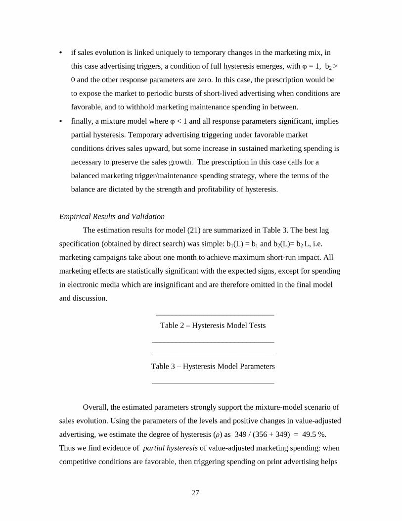
The estimation results for model (21) are summarized in Table 3. The best lag

specification (obtained by direct search) was simple: b1(L) = b1 and b2(L)= b2 L, i.e.

marketing campaigns take about one month to achieve maximum short-run impact. All

marketing effects are statistically significant with the expected signs, except for spending

in electronic media which are insignificant and are therefore omitted in the final model

and discussion.

______________________________

Table 2 – Hysteresis Model Tests

_______________________________

_______________________________

Table 3 – Hysteresis Model Parameters

_______________________________

Overall, the estimated parameters strongly support the mixture-model scenario of

sales evolution. Using the parameters of the levels and positive changes in value-adjusted

advertising, we estimate the degree of hysteresis (ρ) as 349 / (356 + 349) = 49.5 %.

Thus we find evidence of partial hysteresis of value-adjusted marketing spending: when

competitive conditions are favorable, then triggering spending on print advertising helps

28

propel sales to higher levels in the evolutionary path of the product. At the same time,

some maintenance spending will be needed to sustain the path of growth, so the success

associated with higher revenues comes with a burden on future marketing spendingxvi.

How robust are these partial-hysteresis results against other possible explanations

? First, in unreported experiments, we find no statistical evidence of hysteresis in other

elements of the marketing mix on which data were available. Second, a symmetry test

reveals that advertising hysteresis exists only in marketing campaigns, not in spending

cuts. Furthermore, the hysteretic advertising effects lose their statistical significance

when the interacting variable (Q) is omittedxvii. This finding is in line with Simon’s

(1997) conjecture that marketing spending in and of itself does not generate hysteresis.

For the company under study, it implies that, the more it engages in product- and

technology enhancement that creates even temporary competitive advantage, the more it

can generate long-term benefits from its marketing spending.

We further test for the presence of reverse causation that could bias our hysteresis

estimates. A Hausman specification test reveals no endogeneity in advertising spending.

Furthermore, print advertising spending does not Granger cause value shocks, and value

shocks do not Granger cause print advertising spending.

Lastly, we conduct a validation test of the partial hysteresis result by examining

the stability of the parameters b1 and b2 (and, therefore, ρ) in (21), estimated over

various time subsamples. Indeed, if we wish to derive optimal spending rules from the

presence of hysteresis, it is important to establish that the hysteresis effect can be

replicated over time. The test computes recursive estimates of hysteresis along with the

other response parameters, starting from a minimum sample size of 30 observations, and

expanding the sample one observation at a time. We find that the time path of the 13

successive estimates of ρ is centered around 58.7 %, with a standard deviation of 4.9 %.

Furthermore, all 26 parameter estimates have the correct sign.

The conclusion of these validation tests is that our sample estimates indeed

capture a hysteresis effect that is robust and replicable over time, and that is therefore

amenable to optimization.

29

Long-term Marketing Spending Implications

The long-term profitability impact of hysteresis and trigger-maintenance

marketing spending can be demonstrated by comparing the required multi-period

marketing budgets under two scenarios, with and without hysteresis. Suppose that, given

the market conditions near the end of the evolutionary path in our example, sales are

targeted to grow to 50,000 monthly units for the next six months. Without hysteresis, the

monotonic sales-response function would dictate that monthly advertising spending of

$148,400 would be required to achieve that goal (obtained by log inversing the response

function), holding prices and other market conditions constant. The required marketing

budget over the planning horizon is therefore $890,400.

By contrast, our partial hysteresis finding (ρ = 0.495) indicates that such

repetitive spending is not necessary. A superior strategy is to take advantage of the

(partial) investment quality of marketing spending: trigger sales to the desired target

level, and keep it there for six months with a reduced marketing maintenance budget.

While we do not have the exact data on profit margin π and marketing cost function δ, we

know that the product is profitable and we use a conservative estimate of profit hysteresis

γ = 0.5. Under this scenario, we can apply equation (20) to the sales target and the unique

sales path leading up to the present. We find that the optimal trigger investment is

$181,100, and the maintenance spending is $85,200. As a result, the semi-annual profit

increase due to hysteresis is $890,400 - $181,100 - 5 * $85,200 = $283,300, or

approximately 32 % of the original budget. The longer the planning horizon and/or the

more favorable the current market conditions, the more economic benefits will accrue.

As proposed in the introduction to the paper, the long-run profitability implications of

hysteresis can indeed be meaningful.

Conclusions

When temporary marketing activities affect the long-term evolution of sales, a

condition called hysteresis is created. Hysteresis in marketing changes the prevailing

resource allocation paradigm. Instead of allocating marketing investments in accordance

with a one-to-one mapped marketing-sales function, hysteresis creates two distinct roles

30

of marketing spending: one is triggering sales performance to higher levels, the other is

maintenance spending to sustain these higher levels. As such, hysteresis is economically

beneficial to managers aspiring to meet their sales growth targets.

The intuition behind this economic benefit is as follows. Absent marketing

hysteresis, the firm’s achievement of sustained sales growth requires permanently higher

(repetitive) marketing budgets, notwithstanding possible uneven short-term allocations

such as pulsing or chattering. In these cases, the one-to-one functional relationship

between sales and marketing spending drives the allocation rules. By contrast, under full

hysteresis, all of this repetitive spending is replaced by a single upfront temporary

investment and the resulting sales increases are self-sustaining. Finally, under partial

hysteresis, a portion of the required permanent marketing spending can be substituted by

the upfront trigger investment. The full or partial substitution of permanent marketing

spending by temporary investments gives hysteresis its powerful economic benefit to the

marketer. Indeed, an argument could be made that hysteresis creates long-term assets out

of current marketing expenditures and that these expenditures should therefore be

capitalized for accounting and financial reporting purposes.

Our paper has formalized these fundamental results in two ways. First, we have

shown how the strength of marketing-induced hysteresis, ρ, can be measured on a simple

zero-to-one scale from readily available sales and marketing-mix time-series data.

Second, we have derived the long-term optimal marketing resource allocation rules in

function of γ, a metric that combines response hysteresis ρ with profitability. These rules

split any given marketing budget in a triggering and a sustenance allocation, and they can

also help set the unconstrained optimal level of triggering and maintenance. Using

dynamic programming, we have obtained exact expressions for the amount of triggering

that is needed to replace costly marketing maintenance budgets.

One corollary of hysteresis is that future marketing spending optimally depends

not only on the intended sales and profit target, but also on the historical time path of

sales. Furthermore, the more a brand’s historical sales success has depended on past

initial marketing spending, the more will have to be spent to reach higher future targets.

These findings provide new quantitative evidence of the role of past sales evolution in the

determination of future sales targets and required marketing budgets.

31

Our paper has focused on the analytical and empirical modeling of marketing

hysteresis, without formally investigating the market conditions or behavioral rationales

that lead to its existence. Some conditions that favor hysteresis have already been

hypothesized in the literature, but until they are thoroughly tested and disseminated, we

should not expect management to fully anticipate hysteresis, and allocate their marketing

resources accordingly. Instead, management should rely maximally on current

information on sales or other performance measures and, when hysteresis is detected, be

prepared to act on it quickly. Meanwhile, both behavioral and marketing strategic

research is needed in order to create a knowledge base for hysteresis and its ramifications.

Specific topics include the hysteresis of qualitative marketing initiatives, segment

response differences, impact of competition, and the combination of hysteretic and

pulsing effects of marketing. Our empirical investigation provides evidence in one

important case: when, in the course of a product’s evolution, there are windows of

opportunity created by the product’s high customer value relative to the competition, then

temporary advertising triggering in support of the product can have a beneficial hysteretic

effect on sales, and this effect allows management to shift permanent marketing budgets

into temporary ones. The resulting gains in marketing effectiveness and long-term

profitability can be substantial.

32

Bibliography

Bellman, R. E. and S. E. Dreyfus (1962), Applied Dynamic Programming. PrincetonUniversity Press.

Blattberg, Robert C. and John Deighton (1996), “Manage Marketing by the CustomerEquity Test,” Harvard Business Review, July-August, 136-144.

Bronnenberg, Bart J., Vijay Mahajan and Wilfried R. Vanhonacker (2000), "TheEmergence of Market Structure in New Repeat-Purchase Categories: A DynamicApproach and an Empirical Application," Journal of Marketing Research, 37 (February),16-31.

Chow, Gregory C. (1997). Dynamic Economics: Optimization by the Lagrange Method.New York: Oxford University Press.

Dekimpe, Marnik and Dominique M. Hanssens (1995a), “The Persistence of MarketingEffects on Sales,” Marketing Science, 14:1 (Winter), 1-21.

Dekimpe, Marnik and Dominique M. Hanssens (1995b), “Empirical GeneralizationsAbout Market Evolution and Stationarity,” Marketing Science, 14:3 (Part 2 of 2), G109-21.

Dekimpe, Marnik and Dominique M. Hanssens (1999), “Sustained Spending andPersistent Response: A New Look at Long-term Marketing Profitability,” Journal ofMarketing Research, 36 (November), 1-31.

Dekimpe, Marnik, Dominique M. Hanssens, and Jorge M. Silva-Risso (1999), "Long-runEffects of Price Promotions in Scanner Markets," Journal of Econometrics, 89, 269-291

Dorfman, Robert and Peter Steiner (1954), “Optimal Advertising and Optimal Quality,”American Economic Review, 44 (December), 826-36.

Fishbein, Martin and Icek Ajzen (1975). Belief, Attitude, Intention, and Behavior : AnIntroduction to Theory and Research. Reading, MA: Addison-Wesley.

Fortin, Pierre (1991), “The Phillips Curve, Macroeconomic Policy, and the Welfare ofCanadians,” Canadian Journal of Economics, 24:4, 774-803.

Franses, Philip Hans (1994), “Modeling New Product Sales: An Application ofCointegration Analysis”, International Journal of Research in Marketing, 11, 491-502.

33

Franz, Wolfgang, Editor (1990), “Special Issue on Hysteresis Effects in EconomicModels,” Empirical Economics, 15:2.

Gordon, Robert J. (1989), “Hysteresis in History: Was there Ever a Phillips Curve?”American Economic Review, 79:2 (May), 220-225.

Hamilton, James D. (1994). Time Series Analysis. Princeton, NJ: Princeton UniversityPress.

Hanssens, Dominique M., Leonard J. Parsons and Randall L. Schultz (2001). MarketResponse Models, Second Edition. Boston: Kluwer Academic Publishers.

Horsky, Dan and Leonard S. Simon (1983), “Advertising and the Diffusion of NewProducts,” Marketing Science, 2 (Winter), 1-17.

Lambin, Jean-Jacques, Philippe Naert and Alain Bultez (1975), “Optimal MarketingBehavior in Oligopoly,” European Economic Review, 6, 105-28.

Little, John D.C. (1979), “Aggregate Advertising Models: The State of the Art,”Operations Research, 29, 629-67.

Liu, Donald J. and Olan D. Forker (1990), "Optimal Control of Generic Fluid MilkAdvertising Expenditures," American Journal of Agricultural Economics, November,1047-1055.

Naik, Prasad A., Murali K. Mantrala and Alan G. Sawyer (1998), “Planning MediaSchedules in the Presence of Dynamic Advertising Quality,” Marketing Science, 17:3,214-235.

Nerlove, Marc and Kenneth J. Arrow (1962), “Optimal Advertising Policy Under Dy-namic Conditions,” Economica, 29 (May), 129-42.

Ouyang, Ming (1997), “A Study of Hysteresis in the Open Canadian Economy,”unpublished Ph.D. dissertation, University of Manitoba.

Powers, Keiko, Dominique M. Hanssens, Yih-Ing Hser, and M. Douglas Anglin (1991),“Measuring the Long-term Effects of Public Policy: The Case of Narcotics Use andProperty Crime,” Management Science, 37, 6 (June), 627-44.

Rayleigh, Lord (1887), "On the Behaviour of Iron and Steel Under the Operation ofFeeble Forces," Philosophy Magazine, 23, 225-248

Sargent, Thomas (1987 ). Dynamic Macroeconomic Theory. Harvard University Press.

Sasieni, Maurice W. (1971), “Optimal Advertising Expenditure,” Management Science,18 (December), 64-72.

34

Sasieni, Maurice W. (1989), “Optimal Advertising Strategies,” Marketing Science, 8:4(Fall), 358-70.

Schmalensee, Richard (1972). The Economics of Advertising. New York: North-Holland.

Sethi, Suresh P. (1977), “Optimal Advertising for the Nerlove-Arrow Model Under aBudget Constraint,” Operations Research Quarterly, 28:3, 638-93.

Simon, Hermann (1982), “ADPULS: An Advertising Model with Wearout andPulsation,” Journal of Marketing Research, 19 (August), 352-63.

Simon, Hermann (1997), “Hysteresis in Marketing — A New Phenomenon?” SloanManagement Review, 38:3 (Spring), 39-49.

Tresca, H. (1864), "Memoire sur L'ecoulement des Corps Solides Soumis de FortesPressions," C. R. Acad. Sci. Paris, 59, 754

Varian, Hal R. (1992). Microeconomic Analysis, 3rd ed. New York: Norton.

Vidale, M. L. and H. B. Wolfe (1957), “An Operations Reseach Study of Sales Responseto Advertising,” Operational Research Quarterly, 5 (June), 370-81.

Welam, Ulf Peter (1982), “Optimal and Near Optimal Price and Advertising Strategies,”Management Science, 28 (November), 1313-27.

35

APPENDIX A

PARAMETER IDENTIFICATION

Assume the optimal allocation takes the form of♣:

Where I and H are unknown constants. Then:

We impose: H = 1, then:

Combine (A1) with the (binding) constraint (12), we have:

Rearrange items:

From the (binding) constraint (12) we know:

Therefore:

Combine it with (A1) and (A3), we have:

♣ This conjecture can be easily verified by substituting (A5) back into it.

)(ln)1(ln tAHItA MM +=+

IHM

M

etA

tA =+))((

)1(

)1()1(

)( Ae

tAtA

I

MM +=

)2()()1()1()()( AtAetAtAtA MIMMT −=+−=

)3(1

)()( A

e

tAtA

I

TM

−=

)1()()1( −=+− tAtAtA MMT

)()1()1( tAtAtA MMT −−=−

36

That is:

Where ρ is a constant.

Substitute (A3) and (A4) into our conjecture (14), (and note AT = AT(t), AT(-1) = AT(t-1),

AM = AM(t), (AM)' = AM(t+1)), the right-hand-side of (14) becomes:

Then the first-order-condition yields:

Rearrange items, we get:

Substitute (A5) back to the RHS expression, and rearrange items give us:

Therefore we can identify:

Substitute (A6) back to (A5), we get:

−

−=−I

T

I

IT

e

tA

e

etA

1

)(1)1(

)4()()1( AtAtA TT ρ=−

TTMTT AAAAARHS Ψ+−Ω+Φ++= βββργ )ln(lnln

(*)1

TMTTT AAAAA −Ω=Ψ++ ββγ

)5()()'(

1

1)(

**

*

AAAA

and

AA

TMM

MT

−=

+Ω+Ψ++Ψ+=

γββγβ

γββ

=ΨΩ+Ψ+=Ω 1

)6(1

1A

ββγ

−+=Ω

37

where B is the budget, and γ is the profit-weighted hysteresis parameter.

Q.E.D.

**

*

)()(

)1(1

1)1(1

1)(

TM

T

ABA

BBA

−=

−

+

+=−+++= β

γβγβ

γβγγ

38

APPENDIX B

DETERMINING UNCONSTRAINED TRIGGERING

To achieve a targeted level of sales, St, how much marketing spending, At, is

necessary? A general marketing hysteresis response model can be characterized as:

St = f(g(At, At-1, γ))

Where g is goodwill, which serves as an intermediate variable, and γ is the hysteresis

parameter. The time index t = 1, 2, …. The inverse of this function gives us:

At* = f-1(St, St-i, A0, γ), i=1, 2, 3, … (B0)

This relationship says that the triggering is determined by a targeted level of sales, St, all

previous sales, St-i, as well as the degree of hysteresis, γ, and the initial condition, A0.

With assumptions of a competitive market condition (i.e., the firm is a price taker), fixed

unit production costs, and a Cobb-Douglas specification for the goodwill function, the

hysteresis sales-marketing response function takes the form of Equation (11):

St = lnAt + γ lnAt-1, t = 1, 2, 3, …

Therefore we have the following:

In order to cancel out items of lnAi, i=1, 2, …, and get an expression like (B0), we use a

weight factor (-γ)t-i to weigh and sum Equations (Bt), (Bt-1), .. (B2), (B1):

(Bt) - γ(Bt-1) + γ2(Bt-2) - γ3(Bt-3) + … + (-γ)t-2(B2) + (-γ)t-1(B1)

The summation gives us:

)(lnln

)1(lnln

...

)2(lnln

)1(lnln

1

211

122

011

BtAAS

BtAAS

BAAS

BAAS

ttt

ttt

−

−−−

+=−+=

+=+=

γγ

γγ

39

And

Let RHS = LHS, and rearrange items:

Therefore the triggering is:

The triggering amount is jointly determined by the target sales level, St, the system's

initial condition, A0, the history of market performance, St-i, and of course, the degree of

profit hysteresis, γ.

∑−

=−

−−−−−

−Σ+=

−+−++−+−1

1

11

22

33

22

1

)(

)()(...

:

t

iit

it

tttttt

SS

SSSSSS

LHS

γ

γγγγγ

01 ln)(ln

:

AA

RHSt

t−−+ γ

∑−

=−−Σ++−=

1

10

)(ln)(lnt

iit

it

tt

SSAA γγ

−Σ+−+= ∑−

=−

1

10

* )(ln)(expt

iit

ittt

SASA γγ

Table 1: Hysteresis and Its DevelopmentYear Investigator Discipline Object Methodology Contribution Application

1887* L. Rayleigh Physics Ferromagnetic Analytical model describingcurrent-magnetic intensity

Discovery of ferric-memorycapacity

All kinds of electrical andelectronic appliances andequipment

1864* H. Tresca Mechanics Plastics Stress analysis Theory of elastic and plasticproperties

Various material & structuralengineering applications

1979 J. Little OperationsReserach

AdvertisingEffectiveness

Conceptual description Argues that advertising mayexhibit hysteresis

Introduces the concept tomarketing

1983 P. Jones OperationsResearch

Sales-advertisingrelationship

Static game theory Shows existence of hysteresis inasymmetric games

Introduces the concept toeconomics and businessdisciplines

1986 O. Blanchard & L.Summers

Economics Labour markets Theoretical analysis Explains persistent highunemployment in Europe

Supports New Keynesian multi-equilibria theory

1987 R. Baldwin,A. Dixit, &P. Krugman

Economics International Trade Theoretical analysis Explains persistence in the UStrade deficit

Provides theoretical rationale forPresident Reagan's trade policy

1989 R. Gordon Economics Labour markets Empirical analysis Estimates Phillips curve invarious OECD economies

Finds traces of hysteresis in theunemployment/inflationrelationship

1995,1999

M. Dekimpe & D.Hanssens

Marketing Sales-marketingrelationship

Multivariate Time-Series Analysis Unit- root based diagnostics forpersistent marketing effects

Long-run marketing effects onsales, profits

1997 H. Simon Marketing MarketingDecision Making

Conceptual description Call for awareness Encourages more studies in thefield

2001 Current Study Marketing MarketingDecision Making

Econometric & theoreticalanalysis

Quantifies strength of marketinghysteresis & optimal resourceallocation

Marketing resource allocation forlong-run profitability

* Publication date of a formal model, though earlier studies had already made conceptual descriptions. Due to its importance as a theoretical framework and in practical application, hysteresis studies in thesedisciplines continue to appear.

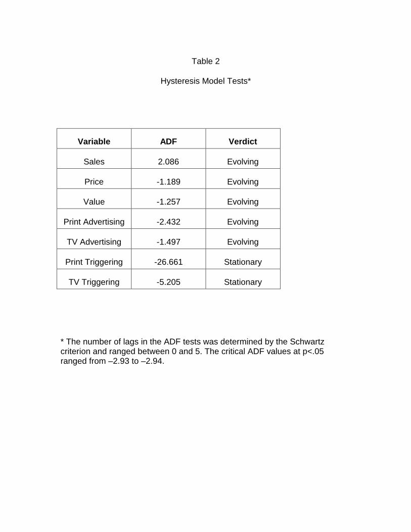
Table 2

Hysteresis Model Tests*

Variable ADF Verdict

Sales 2.086 Evolving

Price -1.189 Evolving

Value -1.257 Evolving

Print Advertising -2.432 Evolving

TV Advertising -1.497 Evolving

Print Triggering -26.661 Stationary

TV Triggering -5.205 Stationary

* The number of lags in the ADF tests was determined by the Schwartzcriterion and ranged between 0 and 5. The critical ADF values at p<.05ranged from –2.93 to –2.94.

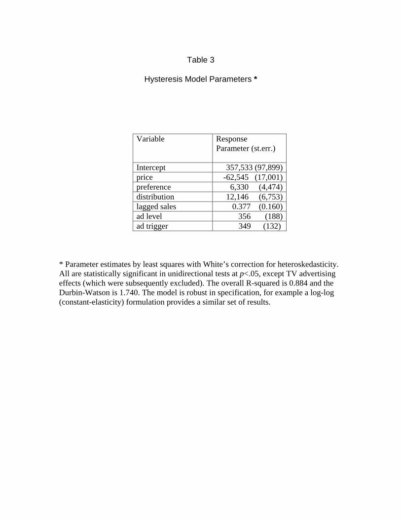
Table 3

Hysteresis Model Parameters *

Variable ResponseParameter (st.err.)

Intercept 357,533 (97,899)price -62,545 (17,001)preference 6,330 (4,474)distribution 12,146 (6,753)lagged sales 0.377 (0.160)ad level 356 (188)ad trigger 349 (132)

* Parameter estimates by least squares with White’s correction for heteroskedasticity.All are statistically significant in unidirectional tests at p<.05, except TV advertisingeffects (which were subsequently excluded). The overall R-squared is 0.884 and theDurbin-Watson is 1.740. The model is robust in specification, for example a log-log(constant-elasticity) formulation provides a similar set of results.

Figure 1. Full and Partial Hysteresis

time

$Full hysteresis

$

sales

sales

time

marketing

marketing

Partial hysteresis

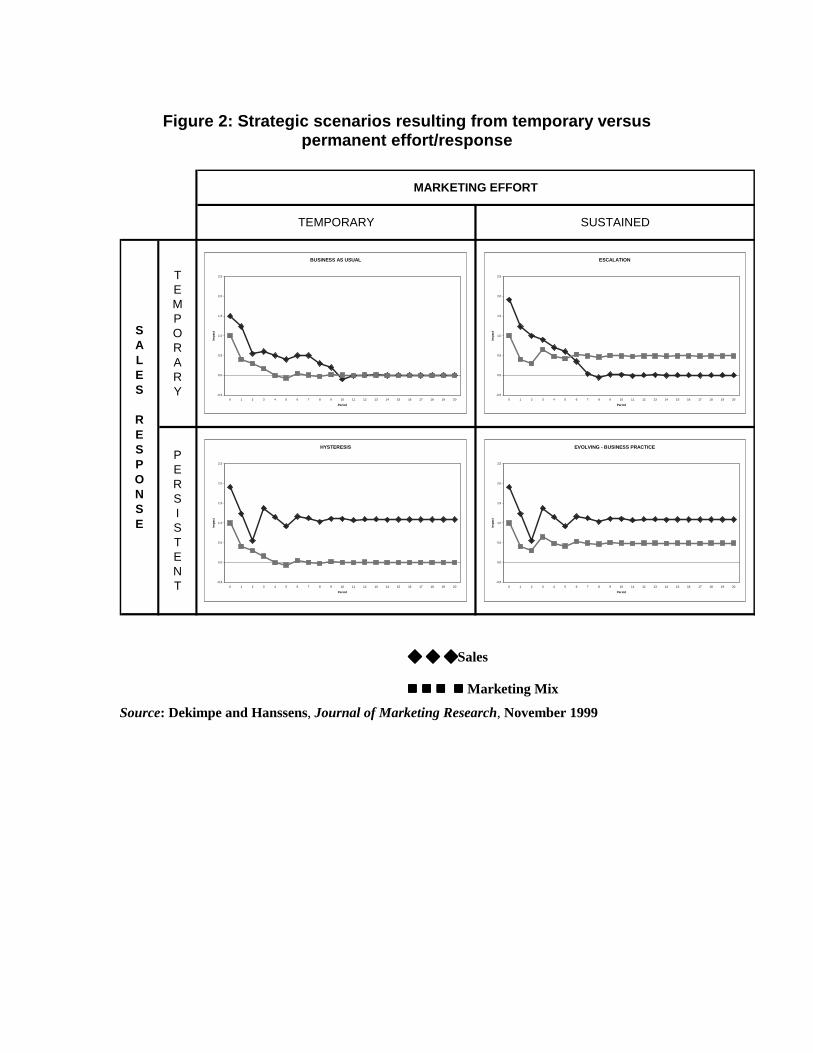
Figure 2: Strategic scenarios resulting from temporary versuspermanent effort/response

SALES

RESPONSE

TEMPORARY

PERSISTENT

MARKETING EFFORT

TEMPORARY SUSTAINED

BUSINESS AS USUAL

-0,5

0,0

0,5

1,0

1,5

2,0

2,5

0 1 2 3 4 5 6 7 8 9 10 11 12 13 14 15 16 17 18 19 20

Period

Impa

ct

ESCALATION

-0,5

0,0

0,5

1,0

1,5

2,0

2,5

0 1 2 3 4 5 6 7 8 9 10 11 12 13 14 15 16 17 18 19 20

Period

Impa

ct

HYSTERESIS

-0,5

0,0

0,5

1,0

1,5

2,0

2,5

0 1 2 3 4 5 6 7 8 9 10 11 12 13 14 15 16 17 18 19 20

Period

Impa

ct

EVOLVING - BUSINESS PRACTICE

-0,5

0,0

0,5

1,0

1,5

2,0

2,5

0 1 2 3 4 5 6 7 8 9 10 11 12 13 14 15 16 17 18 19 20

Period

Impa

ct

Sales

!!!! !!!! !!!! !!!! Marketing Mix

Source: Dekimpe and Hanssens, Journal of Marketing Research, November 1999

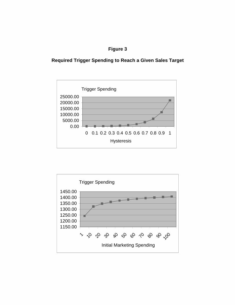
Figure 3

Required Trigger Spending to Reach a Given Sales Target

Trigger Spending

0.005000.00

10000.0015000.0020000.0025000.00

0 0.1 0.2 0.3 0.4 0.5 0.6 0.7 0.8 0.9 1

Hysteresis

Trigger Spending

1150.001200.001250.001300.001350.001400.001450.00

1 10 20 30 40 50 60 70 80 90 100

Initial Marketing Spending

Figure 4. Sales and Marketing Spending

Figure 5. Price and Competitive Value

0

200

400

600

800

1000

1991 1992 1993 1994 1995

SALES PRINTAD

0

10

20

30

40

50

60

70

80

1 3 5 7 9 11 13 15 17 19 21 23 25 27 29 31 33 35 37 39 41 430

100

200

300

400

500

600

Value

Price

Footnotes

i We assume throughout that the order of integration of the data is at most 1 (i.e. evolution)

ii The literature on hysteresis in unemployment and international trade has used a similar approach, see for exampleGordon (1989), Franz (1990), Fortin (1991), Ouyang (1997)

iii In our subsequent development, we will only discuss the case of ρ=0 as absence of hysteresis. The distributed-lagcase (ρ< 0) is not conceptually different

iv A similar treatment may be found in the economics literature, for example, Sargent (1987)

v The Cobb-Douglas function transforms marketing spending, both present and previous, into goodwill monotonically,so the parameters ξ and µ can be transformed to γ (to be consistent with ρ, the hysteresis metric). The Cobb-Douglasfunction requests the summation of the power parameters to be positive, representing their returns to scale. We imposea minus sign in front of µ to serve our purpose, i.e., characterizing our hysteresis metric. In order to make the objectivefunction behave as a standard Cobb-Douglas function (so that dynamic programming can yield meaningful solutions),we subsequently offset the minus sign we imposed, as shown in Equation (11). See Varian (1992) for furtherdiscussion.

vi The lagged-sales term and the presence of exogenous drivers of demand in equation (1) do not affect this definition.

vii The parameter scaling to unity was done for the purpose of simplifying the theoretical analysis. In empirical work, δand π are known, and the response parameters are estimated from the data, so that the unity restriction can be removed.

viii We adopt this notation to show what happens when hysteresis is absent. In the theoretical demonstration, we assumea budget is given as an exogenous variable. Optimal budgeting will be discussed in a later section.

ix Chow (1997) demonstrates that the Bellman equation can be used for two unequal-length periods dynamicprogramming.

x For discussions on how and why the conjecture is set, see the literature on dynamic programming, for exampleBellman and Dreyfus (1962) and Sargent (1987).

xi See Appendix A for details

xii See Appendix A for details

xiii (γ = -1) is an empty point in (AT-γ) space. Although our model allows for negative hysteresis (i.e. γ < 0), that wouldbe irrelevant for optimal resource allocation. Therefore we rule out full negative hysteresis (γ = -1) without affectingthe generality of the solution.

xiv See Appendix B for details

xv If a concavity assumption is imposed on the response function, we could derive a general optimal solution withoutknowing a given budget or a given target level of sales.

xvi We also verified empirically that the levels of sales and marketing are cointegrated, i.e. they co-evolve.

xvii An additional specification test reveals that value shocks (in Q) by themselves do not explain the evolution in sales(i.e. the series are not cointegrated). The statistical details of this and other tests, all of which were conducted at p<.05,are available upon request