Caleffi North America, Inc. 9850 South 54th Street Franklin, WI 53132 T: 414.421.1000 F: 414.421.2878

Dear Hydronic Professional,

Welcome to the 2nd edition of idronics – Caleffi’s semi-annual design journal for hydronic professionals.

The 1st edition of idronics was released in January 2007 and distributed to over 80,000 people in North America. It focused on the topic hydraulic separation. From the feedback received, it’s evident we attained our goal of explaining the benefits and proper application of this modern design technique for hydronic systems.

If you haven’t yet received a copy of idronics #1, you can do so by sending in the attached reader response card, or by registering online at www.caleffi.us. The publication will be mailed to you free of charge. You can also download the complete journal as a PDF file from our Web site.

This second edition addresses air and dirt in hydronic systems. Though not a new topic to our industry, the use of modern high-efficiency equipment demands a thorough understanding of the harmful effects of air and dirt, as well as knowledge on how to eliminate them. Doing so helps ensure the systems you design will operate at peak efficiency and provide long trouble-free service.

We trust you will find this issue of idronics a useful educational tool and a handy reference for your future hydronic system designs. We also encourage you to send us feedback on this issue of idronics using the attached reader response card or by e-mailing us at idronics@caleffi.com.

Sincerely,

Mark Olson General Manager,Caleffi North America, Inc.

A Technical Journalfrom

Caleffi Hydronic Solutions

CALEFFI NORTH AMERICA, INC3883 W. Milwaukee Rd

Milwaukee, Wisconsin 53208 USA

Tel: 414-238-2360FAX: 414-238-2366

E-mail: idronics@caleffi.comWebsite: www.caleffi.us

To receive future idronics issues FREE, register online www.caleffi.us

Dear Hydronic Professional,

Welcome to the 8th edition of idronics, Caleffi’s semi-annual design journal for hydronic professionals.

A hydronic system can be installed with the latest heat sources, heat emitters, and other hardware, but without proper balancing, it is unlikely to deliver optimal comfort and energy efficiency.

In this issue we explore the purpose and benefits of balancing, as well as its underlying theory. We go on to review the different types of balancing devices available in the market, and show how to select and apply them.

We encourage you to send us feedback on this issue of idronics by e-mailing us at idronics@caleffi.com.

If you are interested in previous editions of idronics, please go to www.caleffi.us where they can be freely downloaded. You can also register on-line to receive future hard copy issues.

Sincerely,

General Manager

3 WHY IS BALANCING NECESSARY? Consequences Of Imbalanced Hydronic Systems The Purpose Of Balancing

6 FUNDAMENTAL CONCEPTS UNDERLYING BALANCING The Effect Of Flow Rate On Heat Output Thermal Models For Heat Emitters Computer Simulation Of Virtual Hydronic Systems Each Crossover Affects Other Crossovers Flow Coefficient Cv Reverse Return Piping

16 TYPES OF BALANCING DEVICES Globe Valves Equal Percentage Valves Differential Pressure Type Balancing Valves Sizing A Differential Pressure Type Balancing Valve Direct Reading Balancing Valves Pressure Independent Balancing Valves (PIBV)

28 BALANCING PROCEDURES FOR SYSTEMS USING MANUALLY SET BALANCING VALVES Balancing Basics Determining Crossover Flow Rates Balancing Using Preset Method

Balancing Using Compensated Method Balancing Multiple Branch Systems Balancing Procedure For Manifold Systems

46 SYSTEMS USING PRESSURE-INDEPENDENT BALANCING VALVES Application Of PIBVs Using PIBVs With Variable Speed Circulators Energy Savings Using Variable Speed Circulator And PIBVs

51 BALANCING INJECTION MIXING SYSTEMS Injection Mixing With 2-Way Modulating Valves Injection Mixing With A Variable Speed Circulator

55 SUMMARY

56 Appendix A: Piping Symbol Legend

57 Appendix B: Head Loss Calculation Method

59 Appendix C: Thermal Model For A Radiant Panel Circuit

60 Appendix D: Density of Water

Caleffi North America, Inc.3883 W. Milwaukee RdMilwaukee, Wisconsin 53208T: 414.238.2360 F: 414.238.2366

10%

Cert no. XXX-XXX-XXXX

© Copyright 2011 Caleffi North America, Inc.

Printed: Milwaukee, Wisconsin USA

INDEX

Disclaimer: Caleffi makes no warranty that the information presented in idronics meets the mechanical, electrical or other code requirements applicable within a given jurisdiction. The diagrams presented in idronics are conceptual, and do not represent complete schematics for any specific installation. Local codes may require differences in design, or safety devices relative to those shown in idronics. It is the responsibility of those adapting any information presented in idronics to verify that such adaptations meet or exceed local code requirements.

3

1: WHY IS BALANCING NECESSARY?

Hydronic heating systems have the potential to deliver a precise rate of heating when and where its needed within a building.

The key word in the previous sentence is potential. Without proper design, and proper balancing, that potential seldom becomes reality.

In the context of hydronics, balancing refers to the adjustment of valves to direct flow within a heating or cooling system so that desired interior comfort levels are achieved and maintained in all areas served by the system.

Previous issues of idronics have discussed the proper design of a wide range of hydronics systems. Many of these systems, including 2-pipe direct return, 2-pipe reverse return, and manifold-based distribution, use parallel circuits to deliver a portion of the total system flow rate to either individual zones within a building or individual heat emitters.

Ideally, every zone or heat emitter in such systems would be identical to the others. Each would need to deliver the same rate of heating, and each would have identical branch piping. Thus, each would need an equal percentage of the total system flow rate.

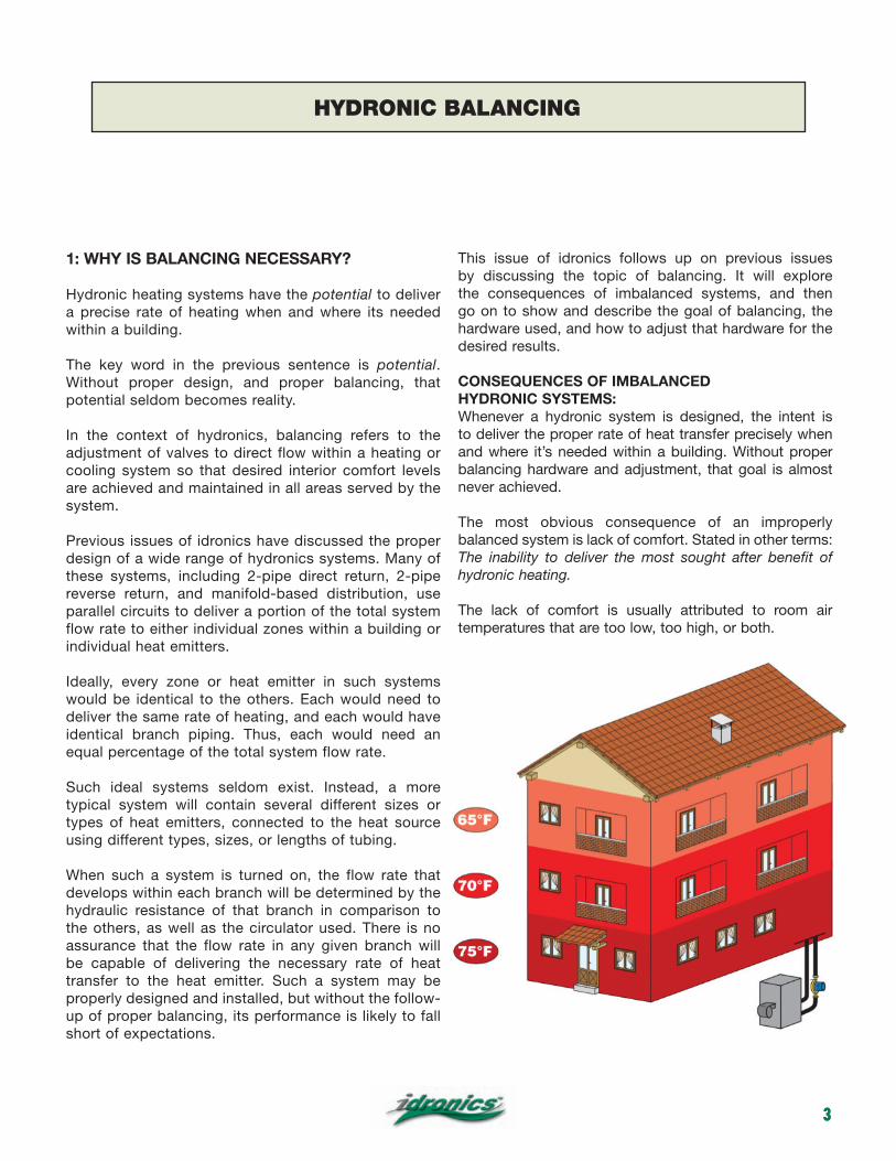
Such ideal systems seldom exist. Instead, a more typical system will contain several different sizes or types of heat emitters, connected to the heat source using different types, sizes, or lengths of tubing.

When such a system is turned on, the flow rate that develops within each branch will be determined by the hydraulic resistance of that branch in comparison to the others, as well as the circulator used. There is no assurance that the flow rate in any given branch will be capable of delivering the necessary rate of heat transfer to the heat emitter. Such a system may be properly designed and installed, but without the follow-up of proper balancing, its performance is likely to fall short of expectations.

This issue of idronics follows up on previous issues by discussing the topic of balancing. It will explore the consequences of imbalanced systems, and then go on to show and describe the goal of balancing, the hardware used, and how to adjust that hardware for the desired results.

CONSEQUENCES OF IMBALANCED HYDRONIC SYSTEMS:Whenever a hydronic system is designed, the intent is to deliver the proper rate of heat transfer precisely when and where it’s needed within a building. Without proper balancing hardware and adjustment, that goal is almost never achieved.

The most obvious consequence of an improperly balanced system is lack of comfort. Stated in other terms: The inability to deliver the most sought after benefit of hydronic heating.

The lack of comfort is usually attributed to room air temperatures that are too low, too high, or both.

HYDRONIC BALANCING

4

Wide variations in interior temperature often lead to problems beyond the lack of comfort.

When some areas of a building cannot be warmed to the desired room air temperature, the following problems can develop:

• Frozen piping in the building’s hydronic system, its plumbing system, or both

• Shrinkage cracks in wood and drywall surfaces

• Slow drying of wetted surfaces

• Condensation on windows

• Growth of mold and mildew

• Increased potential for respiratory illnesses, and aggravation of other medical conditions such as arthritis

5

• Poor environment for some interior plants.

Rooms that remain at higher than desired temperatures also create problems, such as:

• Poor mental alertness

• Wasted heating energy due to higher heat losses

• Increased air leakage through building envelope• Increased probability of low interior humidity• Premature spoilage of food

Other undesirable conditions that can result from improperly balanced systems include:

• High flow velocities in piping components creating noise and possible erosion

• Excessive energy use by circulators due to overflow conditions

• Circulators that operate at low efficiency

• Circulators that operate at high differential pressure, increasing potential for thrust damage of bushings or bearings

• Circulators that operate at high flow rates and low differential pressure may experience motor overloading

• Possible “bleed through” flow in zones that are supposed to be off.

THE PURPOSE OF BALANCING:Most hydronic heating professionals agree that balanced systems are desirable. However, opinions are widely varied on what constitutes a balanced system. The following are some of the common descriptions of a properly balanced system:

• The system is properly balanced if all simultaneously operating circuits have the same temperature drop.

• The system is properly balanced if the ratio of the flow rate through a branch circuit divided by the total system flow rate is the same as the ratio of the required heat output from that branch divided by the total system heat output.

6

• The system is properly balanced if all branch circuits are identically constructed (e.g., same type, size and length of tubing, same fittings and valves, same heat emitter).

• The system is properly balanced if constructed with a reverse return piping layout.

• The system is properly balanced if the installer doesn’t receive a complaint about some rooms being too hot while others are too cool.

While some of these definitions of proper balancing are related, none of them is totally correct or complete. It follows that any attempt at balancing a system is pointless without a proper definition and “end goal” for the balancing process.

In this issue of idronics, the definition of a properly balanced system is as follows:

A properly balanced hydronic system is one that consistently delivers the proper rate of heat transfer to each space served by the system.

At first this definition may seem simplistic, but it ultimately reflects the fundamental goal of installing any heating system.

2: FUNDAMENTAL CONCEPTS UNDERLYING BALANCING

Balancing hydronic systems requires simultaneous changes in the hydraulic operating conditions (e.g., flow rates, head losses, pressure drops), as well as the thermal operating conditions (e.g., fluid temperatures, room air temperatures) of the system. These operating conditions will always interact as the system continually seeks both hydraulic equilibrium and thermal equilibrium. The operating conditions will also be determined, in part, by the characteristics of the heat emitters and circulator used in the system.

Considering that there are often hundreds, if not thousands, of piping and heat emitter components in a system, and that nearly all of them have some influence on flow rates and heat transfer rates, it is readily apparent that a theoretical approach to balancing can be complicated.

This section discusses several of the fundamentals that collectively determine the balanced (or unbalanced) condition of every hydronic system. All these fundamentals can be dealt with mathematically. However, in many cases this is not necessary. Instead,

it is sufficient to have a clear understanding of how and why certain conditions exist or develop with a system, even without numbers to show the exact changes. Such an understanding can guide the balancing process in the field, and help the balancing technician avoid mistakes or incorrect adjustments that delay or prevent a properly balanced condition from being attained.

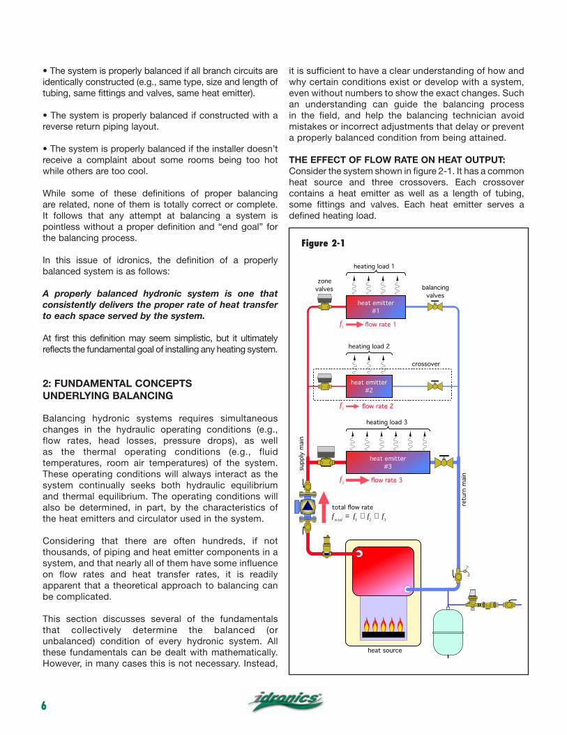
THE EFFECT OF FLOW RATE ON HEAT OUTPUT:Consider the system shown in figure 2-1. It has a common heat source and three crossovers. Each crossover contains a heat emitter as well as a length of tubing, some fittings and valves. Each heat emitter serves a defined heating load.

VENT

supp

ly m

ain

retu

rn m

ain

heat emitter #3

heat emitter #1

heat emitter #2

flow rate 3

flow rate 2

flow rate 1

total flow ratef to tal = f1 + f2 + f3

f3

f1

f2

balancing valves

zone valves

heating load 1

heating load 2

heating load 3

crossover

heat source

Figure 2-1

7

In some systems, two or more of the crossovers may contain the same heat emitter, or be piped with the same size and type of tubing. However, this is not always going to be the case. In the most general sense, every branch can contain different heat emitters, and different piping components.

The rate of heat transfer from each heat emitter depends on its size, its inlet fluid temperature, and the flow rate through it.

Because all the crossovers in figure 2-1 are supplied from a common supply main, and making the reasonable assumption that heat loss from the supply main is relatively small in comparison to heat output from the heat emitter, it follows that each heat emitter is supplied with fluid at approximately the same temperature. This, however, does not guarantee that each heat emitter will have the same heat output, even if the heat emitters are identical.

The flow rate through each heat emitter also affects its heat output. The following principles will always apply:

• The faster a heated fluid passes through a heat emitter, the greater the rate of heat transfer, when all other conditions are equal.

• From the standpoint of heat transfer only, there is no such thing as flow moving too fast through a heat emitter.

Some heating professionals instinctively disagree with the second principle. They argue that because the water moves through the heat emitter at a higher speed, it has less time in which to release its heat. However, the time a given water molecule stays inside the heat emitter is irrelevant in a system with a circulating fluid.

The increased heat output at higher flow rates is the result of improved convection between the fluid and the interior wetted surfaces of the heat emitter. The faster the fluid moves, the thinner the fluid boundary layer between the inside surface of the heat emitter and the bulk of the fluid stream. The thickness of this boundary layer determines the resistance to heat flow. The thinner the boundary layer, the greater the rate of heat transfer.

Another way of justifying this principle is to consider the average water temperature in the heat emitter at various flow rates. Consider the example shown in figure 2-2 where water at 180ºF enters the coil of an air handler unit at different flow rates.

As the flow rate through the coil increases, the temperature difference between its inlet and outlet decreases. This means that the average water temperature in the coil increases, and so does its heat output. This holds true for all other hydronic heat emitters, such as radiant panel circuits, panel radiators and baseboard.

It might seem intuitive to assume that heat transfer from a heat emitter increases in proportion to flow rate through it (i.e., doubling the flow rate through the heat emitter would double its heat output). However, this is not true.

180 ºF140 ºF

average water temperature in coil = 160 ºF

180 ºF157 ºF

average water temperature in coil = 168.5 ºF

180 ºF164ºF

average water temperature in coil = 172 ºF

flow rate = 1 gpm∆T=40ºF, Tave=160ºF

flow rate = 2 gpm∆T=23ºF, Tave=168.5ºF

flow rate = 3 gpm∆T=16ºF, Tave=172ºF

incr

easi

ng h

eat o

utpu

t

Figure 2-2

8

The rate of change of heat output from any hydronic heat emitter is a strong function of flow rate. At low flow rates, heat output rises rapidly with increasing flow, but the greater the flow rate becomes, the slower the rate of increase in heat output.

To illustrate this, consider the situation shown in figure 2-3, which shows the heat output of a typical radiant floor circuit versus the flow rate through it. The circuit is supplied with water at a constant temperature of 105 ºF.

This floor heating circuit’s maximum heat output of 6,860 Btu/hr occurs at the maximum flow rate shown, (2.0 gpm). Decreasing the circuit’s flow rate by 50%to 1.0 gpm decreases its heat output to 6,180 Btu/hr, a drop of only about 10%. Reducing the flow rate to 10% of the maximum value (0.2 gpm) still allows the circuit to release 2,950 Btu/hr, about 43% of its maximum output.

This “non-linear” relationship between heat output and flow is typical of all hydronic heat emitters. It tends to make balancing more complicated than what one might assume. For example, as a technician first begins closing a balancing valve, there is relatively little change on the heat output of the circuit. However, when the balancing valve is only 10 to 25% open, small adjustments will yield relatively large changes in heat output.

THERMAL MODELS FOR HEAT EMITTERS:The analytical models used to determine the effect of both inlet fluid temperature and flow rate vary with each type of heat emitter. They can take the form of one or more

formulas that use inlet fluid temperature and flow rate, along with the characteristics of the heat emitter and its surroundings, to determine the outlet fluid temperature. Once the fluid outlet temperature is known, it can be combined with the inlet temperature and flow rate to determine the total heat output of the heat emitter.

The mathematical form for these models is often complex, and most suitable for evaluation using software. For example, the mathematical model for the fluid temperature at a given location along a finned-tube baseboard is as follows:

Formula 2-1

Where:Tf = fluid temperature at some location L along length of finned-tube element (ºF)Troom = room air temperature entering the baseboard (°F)Tinlet = fluid temperature at inlet of baseboard (ºF)D = density of fluid within baseboard (lb/ft3)c = specific heat of fluid within baseboard (Btu/lb/ºF)ƒ = fluid flow rate through the baseboard (gpm)L = position along baseboard beginning from inlet (ft)B = heat output of the baseboard at 200 °F average water temperature, 1 gpm from manufacturer’s literature* (Btu/hr/ft) The values 0.04, -0.4172, -2.3969319 and 1.4172 are all exponents.

Once the outlet temperature for a baseboard is determined, Formula 2-2 can use it along with the inlet temperature and flow rate to determine the total heat output.

Where:Toutlet = outlet temperature of fluid leaving baseboard (ºF)Tinlet = fluid temperature at inlet of baseboard (ºF)D = density of fluid within baseboard (lb/ft3)c = specific heat of fluid within baseboard (Btu/lb/ºF)ƒ = fluid flow rate through the baseboard (gpm)

For example: Assume a finned-tube baseboard is 20 feet long, located in a room with a floor-level air temperature of 65ºF, and supplied with water at 4 gpm and 180ºF. The baseboard’s manufacturer rates its heat output at 500 Btu/hr/ft when operating with 200 ºF water and a flow rate of 1 gpm. Determine the heat output of this baseboard at the stated conditions, and compare it to the output if the flow rate were reduced to 0.5 gpm.

0

1000

2000

3000

4000

5000

6000

7000

0 0.2 0.4 0.6 0.8 1 1.2 1.4 1.6 1.8 2

heat

out

put (

Btu/

hr)

circuit flow rate (gpm)

2950

61806860

105ºF!constant!

inlet temp.

300 ft x 1/2"!PEX circuit in!

4-inch bare slab, !12-inch!

tube spacing

Figure 2-3Formula 2-1

Formula 2-2

9

The outlet temperature of the baseboard can be determined using Formula 2-1:

The total heat released from the baseboard can now be calculated using Formula 2-2:

Using the same formulas at the reduced flow rate of 0.5 gpm yields an outlet temperature of 153.48ºF, and a total heat output of 6,522 Btu/hr. A comparison of the two operating conditions is shown in figure 2-4.

Notice that the temperature drop along the baseboard increases substantially at the lower flow rate. However, the combined effect of flow rate and temperature drop indicates that heat output dropped about 21%(e.g., from 8,282 to 6,522 Btu/hr). This demonstrates that flow rate has a significant influence on heat transfer, and thus controlling flow rate through balancing can substantially alter heat output.

By repeating these calculations, it is possible to plot heat output of this baseboard as a function of flow rate. Figure 2-5 shows the results over a wider range of flow rate.

This graphs shows a rapid increase in heat transfer at low flow rates, and a relatively slight gain in heat transfer as flow rates rise above approximately 2 gpm.

A similar analytical model for the thermal performance of a radiant panel circuit is given in Appendix C.

COMPUTER SIMULATION OF VIRTUAL HYDRONIC SYSTEMS:A truly accurate engineering model of a hydronic system would contain thermal/hydraulic modeling formulas for each heat emitter, each balancing valve and each piping segment in the system. It would also have a model for the pump curve of the circulator.

Based on the current setting of the balancing valves, the overall simulation would determine the flow rate through each portion of the system, and then use this information within the thermal model of each heat emitter to determine heat output.

The balancing valves within the system could then be adjusted to simulate the change in heat output of each heat emitter. The goal would be to adjust the balancing valves such that the output of each heat emitter is at, or very close to, the necessary design heating load of the space it serves.

180 ºFflow rate:!a. 4 gpm!b. 0.5 gpm

outlet temperature:!a. 175.79 ºF!b. 153.48 ºF20 feet of finned-tube baseboard!

rated at 500 Btu/hr/ft when!supplied with 200 ºF water at 1 gpm

heat output:!a. 8,282 Btu/hr!b. 6,522 Btu/hr

0

1000

2000

3000

4000

5000

6000

7000

8000

9000

0 1 2 3 4 5 6 7 8

heat

out

put (

Btu/

hr)

flow rate (gpm)

180 ºF

20 feet of fin-tube baseboard!rated at 500 Btu/hr/ft when!

supplied with 200 ºF water at 1 gpm

fixed supply temperature

Figure 2-4

Figure 2-5

10

Figure 2-6 shows a screen from one software program that can simulate the thermal and hydraulic behavior of a multiple crossover hydronic system, including the effect of balancing valves and a differential pressure bypass valve.

EACH CROSSOVER AFFECTS OTHER CROSSOVERS:The following statement is another important principle that applies to all hydronic systems with multiple crossovers:

• Adjusting the flow rate in any crossover causes the flow rates in all other crossovers to change.

When the flow rate through a given crossover is reduced, the flow rates in the other crossovers will increase and vice versa. The reduction in flow rate in a given crossover could be the result of partially closing a balancing valve. It might also result from the partial closing of a modulating control valve. Another possibility is a zone valve closing to completely stop flow through the crossover.

The extent of the change in other crossover flow rates could be very minor or very significant depending on the means of differential pressure control (if any) used in the distribution system.

Systems in which differential pressure between a supply manifold and return manifold is held relatively constant by a properly adjusted differential pressure bypass valve, or pressure-regulated circulator operating in constant ∆P mode, will create very minimal changes in crossover flow rates when the flow rate through one crossover is adjusted. This situation is depicted in figure 2-7.

differential!pressure!bypass valve

low flow resistance common piping

changing flow rate in one crossover will have SMALL effect on flow rates in other crossovers

DESIREABLE SITUATION

Figure 2-6

Figure 2-7

11

The converse is also true. Systems that lack differential pressure control, and/or have relatively high hydraulic resistance through the common piping, can create large changes in crossover flow rates when the flow through one crossover is adjusted. An example of such a situation is shown in figure 2-8.

• The “ideal” hydronic distribution system is one in which the flow rate in any given crossover can be adjusted, over a wide range, with no resulting flow changes in the other crossovers.

This condition could only occur if the system maintains a constant differential pressure across all crossovers at all times. Properly adjusted differential pressure bypass valves and pressure-regulated circulators operating in constant differential pressure mode approximate such conditions. Pressure-independent balancing valves (PIBV) can also closely approximate these conditions when properly applied.

FLOW COEFFICIENT Cv:Balancing involves adjusting the flow resistance of valves. The flow resistance created by a valve is often expressed as a value known as the valve’s “Cv.” This value is defined as the flow rate of 60°F water that creates a pressure drop of 1.0 psi through the valve. The valve’s highest Cv value occurs when that valve is fully open. This is called the rated Cv of the valve. For example, a fully open valve with a rated Cv of 5.0 would require a flow rate of 5.0 gpm of 60°F water to create a pressure drop of 1.0 psi across it.

Valve manufacturers list the Cv values of their products in their technical literature. Occasionally Cv values will be listed for devices other than valves.

Formula 2-3 can be used to estimate pressure drop across a valve based on its Cv and the flow rate through it:

where:∆P = pressure drop across the device (psi)D = density of the fluid at its operating temperature (lb/ft3) 62.4 = density of water at 60 °F (lb/ft3) ƒ = flow rate of fluid through the device (gpm)Cv = known Cv rating of the device (gpm)

Example: Estimate the pressure drop across a radiator valve having a rated Cv value of 2.8, when 140 °F water flows through at 4.0 gpm.

Solution: The density of water at 140°F water must first be referenced (see Appendix D). It’s value at 140ºF is 61.35 lb/ft3. This density and the remaining values can now be used in Formula 2-3:

The rated Cv value of a valve is always at its fully open position. As the valve’s stem is closed, the Cv value decreases (e.g., the valve will pass less flow at the same differential pressure). The Cv of any valve approaches zero as the valve stem approaches the fully closed position.

Some balancing procedures yield a calculated Cv setting for a balancing valve based on the required flow rate through it. Setting a valve to this Cv value requires a known relationship between valve stem position on the resulting Cv value. This relationship is often published for valves designed for balancing purposes. It could be a table listing Cv value versus number of turns open, as shown in figure 2-9a, or it might be shown as a graph such as that in figure 2-9b. The sloping red lines in figure 2-9b indicate the number of turns of the valve’s stem from its fully closed position.

high flow resistance common piping

changing flow rate in one crossover will have LARGE effect on flow rates in other crossovers

no differential pressure control

UNDESIREABLE SITUATION

high flow resistance heat source

Figure 2-8

Figure 2-9a

12

REVERSE RETURN PIPING:When two identical devices are piped in reverse return, as shown in figure 2-10, the total flow will divide equally between them without use of balancing valves. Examples of devices that are commonly piped this way include two identical boilers or two identical solar collectors.

However, when more than two identical devices are piped in reverse return, the flow rates do not necessary divide equally among all devices. To illustrate this, consider the reverse return piping assembly shown in figure 2-11.

All the piping segments making up the supply and return mains are built of 1” copper tubing, and all the segments of the mains are equal in length (50 feet). The resistor symbols connected between the mains represent eight identical crossovers, each having the same hydraulic resistances.

Ideally, each of the eight crossovers would pass 1/8th of the total flow rate entering at the lower left inlet (point A), and exiting at the upper right outlet (point P). For this to be true, the total head loss along each of the 8 flow paths between points A and P would have to be the same. To see if this is the case, the head losses of each segment of the supply and return mains have been calculated assuming the total flow does equally divide. These head losses were calculated using methods from Appendix B, and are shown in red in figure 2-11.

The head loss of each piping segment along a given flow path can be added to determine the total head loss along that path. The table in figure 2-12 lists the results

Figure 2-9b

2 gpm

2 gpm

1 gp

m

1 gp

m

Figure 2-10

13

of these additions for each available flow path between points A and P.

Notice that the head losses are not the same along all flow

paths. The paths through the center crossovers (DL, and EM) have the highest total head losses. The paths through the outer crossovers (AI and HP) have the lowest head losses. There is a symmetry to the head loss distribution. For example, (the head loss along path ABC - KLMNOP is the same as along path ABCDEF - NOP). This implies the overflow condition will increase symmetrically as one moves from the center crossovers to the outer crossovers. The flow rates through the center crossovers will be the lowest and those in the outer crossovers will be the highest, as shown in figure 2-13.

The only way to create the same flow rate in each crossover would be to size the supply and return mains for exactly the same head loss per unit of length along their entire length. This concept is represented in figure 2-14.

In theory this is possible, provided tubing could be obtained in virtually any diameter. In reality this is not the case. Finite selections of tubing sizes, and differences in lengths between the mains segments will usually result in some variation in flow rate through more than two identical devices piped in reverse return.

The degree of flow rate variation between crossovers in a reverse return system depends on the magnitude of the head loss through the crossovers versus the head loss along the mains. The following principle applies to reverse return systems with identical crossovers.

8 gpm

8 gpm

∆H = "0.0423 ft

∆H = "0.142 ft

∆H = "0.289 ft

∆H = "0.478 ft

∆H = "0.707 ft

∆H = "0.972 ft

∆H = "1.27 ft

50'x1" 50'x1" 50'x1" 50'x1" 50'x1" 50'x1" 50'x1"

50'x1" 50'x1" 50'x1" 50'x1" 50'x1" 50'x1" 50'x1"

7 gpm 6 gpm 5 gpm 4 gpm 3 gpm 2 gpm 1 gpm

7 gpm6 gpm5 gpm4 gpm3 gpm2 gpm1 gpm

∆H = "0.0423 ft

∆H = "0.142 ft

∆H = "0.289 ft

∆H = "0.478 ft

∆H = "0.707 ft

∆H = "0.972 ft

∆H = "1.27 ft

1 gp

m

1 gp

m

1 gp

m

1 gp

m

1 gp

m

1 gp

m

1 gp

m

1 gp

m

A B C D E F G H

J K L M N O PI

Figure 2-11

A B C D E F G H

J K L M N O PI

Figure 2-12

Figure 2-13

14

• The higher the ratio of the head loss through the crossovers divided by the head loss through the mains, the closer the reverse return system will be to “self-balancing” (e.g., equal flow rates in all crossovers).

The compromise of not having exactly the same flow rate in all identical crossovers is often acceptable, especially when the thermal performance of the devices in the crossovers is not a strong function of flow rate.

Thus, it is common to pipe up to eight solar thermal collectors in a reverse return arrangement and not be concerned about the slight flow rate variations between them. Multiple panel radiators that all serve the same room can also be configured

in reverse return, as shown in figure 2-15.

Reverse return piping systems that “dead end” at the end of a building farthest from the mechanical room require a third pipe to return flow to the mechanical room. This is the upper pipe shown in figure 2-16.

This third pipe must be sized for the full design load flow rate, and thus will likely be the largest pipe in the distribution system. The cost of installing this third pipe will often be higher than using a direct return piping system, especially when balancing valves are needed in either system. The third pipe will also increase uncontrolled heat loss from the system to the building, especially if uninsulated.

8 gpm

8 gpm

7 gpm 6 gpm 5 gpm 4 gpm 3 gpm 2 gpm 1 gpm

7 gpm6 gpm5 gpm4 gpm3 gpm2 gpm1 gpm1

gpm

1 gp

m

1 gp

m

1 gp

m

1 gp

m

1 gp

m

1 gp

m

1 gp

m

A B C D E F G H

J K L M N O PI

all mains piping sized for a constant head loss per unit of length

all mains piping sized for a constant head loss per unit of length

zone valve

panel radiator

2 gpm8 gpm

8 gp

m

8 gp

m

2 gpm

2 gpm 2 gpm 2 gpm

4 gpm 6 gpm

8 gpm

6 gpm 4 gpm 2 gpm2 gpm 2 gpm 2 gpm 2 gpm

To be fully "self-balancing" the devices must have identical hydraulic resistance, AND, the mains piping connecting the devices must be sized for the same head loss per unit of length.

A B

A B C D E F G H

J K L M N O PIheat input

Figure 2-14

Figure 2-15

Figure 2-16

15

Figure 2-17 shows a much more extensive reverse return distribution system that follows around the interior perimeter of a building. This approach eliminates the third pipe described earlier. Systems such as this often have different heat emitters in some of the crossovers. They are also likely to have variations in the lengths of a given pipe size operating at a given flow rate. The reverse return configuration will help in balancing the system, but it does not guarantee the system is self-balancing. In such cases, a balancing device should be installed in each crossover to allow for flow rate adjustments.

The following principles apply to reverse return piping systems:

• Simple, symmetrical reverse return piping of identical devices, that have significantly more hydraulic resistance than the piping mains segments between them, will generally produce small but acceptable variations in flow rate from one device to another. However, more complex systems that contain a variety of pipe sizes, and heat emitters, even when piped in a reverse return manner, should include balancing valves in each crossover.

There are also circumstances when reverse return piping is not needed. One example is shown in figure 2-18.

Although the boilers are identical, and thus should have the same hydraulic resistance, they each have their own

circulator. If the flow resistance of the header piping and hydraulic separator is relatively low (header design flow velocity not over 2 ft/sec), there will be very little variation in flow rate through the boilers, regardless of which boilers are operating. Even when minor flow rate variations do exist, they should not create a problem in such an application.

heat source

balancing valve (on each branch)

differential pressure bypass valve

VENT

Hydro Separator

boiler controller

boiler #1 boiler #2 boiler #3reverse return piping is NOT needed for these boilers

low resistance headers

circulators with integral check valves

Figure 2-17

Figure 2-18

16

3. TYPES OF BALANCING DEVICES

There are several types of devices that can serve as a means of controlling the flow rate in the crossovers of a hydronic distribution system. They range from simple, manually-set devices, such as globe valves and ball valves, to “intelligent” devices called pressure independent balancing valves (PIBV). This section describes each type. Later sections show how each are applied and adjusted.

GLOBE VALVES:One of the “classic” valve designs for regulating flow is known as a globe valve (also sometimes called a “globe-style” valve). It consists of a body that forces flow through several abrupt changes in direction, as seen in figure 3-1. Flow enters the lower valve chamber, flows upward through the gap between the seat and the disc, then exits sideways from the upper chamber. The gap between the disc and the seat determines the hydraulic resistance created by the valve.

Globe valves should always be installed such that flow enters the lower body chamber, and moves upward toward the gap between the seat and disc. This allows the disc to close against the area of higher pressure. Reverse flow through this type of valve can cause unstable flow regulation, cavitation, and noise. All globe valves have an arrow on their body indicating the proper flow direction.

The flat disc that moves upward away from the valve’s seat when the stem is rotated creates a characteristic relationship between flow rate and stem position.

Specifically, it creates what is known as a “quick-opening” characteristic. This implies that flow through the valve increases rapidly as the disc first lifts up from the seat, then continues to rise at progressively slower rates as the disc lifts higher above the seat. This characteristic is illustrated by the red curve in figure 3-2.

Notice that when the valve’s stem reaches the 50% open position, the valve is passing approximately 90% of the flow it will pass when fully open.

The “curvature” of the curve representing the percentage of full flow versus percentage of stem travel depends on the pressure drop across the balancing valve (in its fully open position), versus the pressure drop across the entire crossover in which it is installed. This relationship is depicted in figure 3-3.

The ratio of the pressure drop across the fully open balancing valve divided by the pressure drop across the entire crossover is called “valve authority.” The lower the valve authority of the balancing valve, the more pronounced the curvature of the characteristic shown in figure 3-2. Conversely, the higher the valve authority, the less pronounced the curvature.

It is generally recommended that valves used for regulating heat output by controlling flow rate have a minimum valve authority of 50%. This implies that the pressure drop across the fully open valve should be at least as high as the pressure drop across the remaining piping components in the crossover.

packing nut

stem

packing

bonnet

body

flat disc

handwheel

seat

O-ring seal

0

10

2030

4050

60

7080

90100

0 10 20 30 40 50 60 70 80 90 100

% o

f flow

at c

onst

ant d

iffer

entia

l pre

ssur

e

% of stem travel from closed position

flat disc type valve

higher valve

authority

lower valve

authority

Figure 3-1

Figure 3-2

17

A quick-opening characteristic, when combined with the rapid rise in heat transfer rate at low flow rates, makes the overall relationship between heat output and flow rate very non-linear, and thus more difficult to control, especially at low flow rates.

∆P"balancing"

valve

∆P"mains

zone valve

heat emitterbalancing

valvesu

pply

mai

n

retu

rn m

ain

∆P mains

valve authority = a = ∆P balancing valve

∆P mains

0

10

2030

4050

60

7080

90100

0 10 20 30 40 50 60 70 80 90 100

% o

f flow

at c

onst

ant d

iffer

entia

l pre

ssur

e

% of stem travel from closed position

equal percentage characteristic

0

10

2030

4050

60

7080

90100

0 10 20 30 40 50 60 70 80 90 100

% o

f hea

t out

put

% heat output vs. flow rate!for heat emitter

flow rate vs. % valve stroke!for equal percentage valve

% heat output vs.% valve stroke

% of stem travel from closed position

Figure 3-3

Figure 3-4 Figure 3-5

18

EQUAL PERCENTAGE VALVES:To provide a more proportional relationship between valve stem position and the heat output of the heat emitter being controlled, designers have created valves with different internal “trim.” One of the most common trims gives a valve an “equal percentage characteristic.”

0

10

2030

4050

60

7080

90100

0 10 20 30 40 50 60 70 80 90 100

% o

f flow

at c

onst

ant d

iffer

entia

l pre

ssur

e

% of stem travel from closed position

equal percentage characteristic!(@ constant ∆P and high valve authority)

distorted equal percentage curve!due to lower valve authority

lower valve

authority

seat

equal !percentage !plug!

gap b/w plug and seat!opens slowly at first

gap b/w plug and seat!opens rapidly as valve!stem approaches maximum!lift

logarithmic-shaped plug!(shown closed)

valve seat

Figure 3-6

Figure 3-7

Figure 3-8

19

Flow through this type of valve increases exponentially with upward movement of the stem. Assuming that the differential pressure across the valve is held constant, equal increments of stem movement result in an equal percentage change in the current flow through the valve. For example, moving the stem from 40% open to 50 % open, (a 10 % change), increases flow through the valve by 10 % from its value at 40 % open. Similarly, opening the valve from 50 % to 60 % would again increase flow by 10 % of its value at the 50 % open position.

The overall relationship between flow rate and valve stem position for a valve with an equal percentage characteristic, operated at a constant differential pressure, is shown in figure 3-4.

When a valve with an equal percentage characteristic regulates flow through a heat emitter, the relationship between stem position and heat output is approximately linear, as shown in figure 3-5. As the valve begins to open, the rapid rise in heat output from the heat emitter is compensated for by the slow increase in flow rate through the equal percentage valve. As the valve approaches fully open, the slow increase in heat output is compensated for by rapid increases in flow rate. This is a desirable response for both manually operated balancing valves, as well as motorized 2-way control valves.

The equal percentage characteristic shown in figure 3-4 only holds true if the differential pressure across the valve remains constant, and if the valve’s authority, when installed is at least 50%. If there

are variations in differential pressure across a valve as its stem position changes, or if the valve is applied such that it has low valve authority, the curve shown in figure 3-4 will be distorted in an undesirable direction, as shown in figure 3-6.

A distorted equal percentage characteristic, although not ideal, is still preferable to a quick-opening characteristic when the valve is used to regulate the heat output of a heat emitter. The overall effect will be a heat output characteristic versus valve stem position curve that is not perfectly linear. Heat transfer will increase slightly faster at low flow rates.

Although there are several ways to design valve trim to yield an equal percentage characteristic, two of the most common are:

1. Use a logarithmic-shaped plug as the flow control element2. Use a tapered slot as the flow control element

An example of a valve with a logarithmic-shaped plug is shown in figure 3-7.

Figure 3-8 shows a sequence of an equal percentage plug lifting above its seat. Notice that the higher the plug rises, the faster the gap between the plug and seat increases.

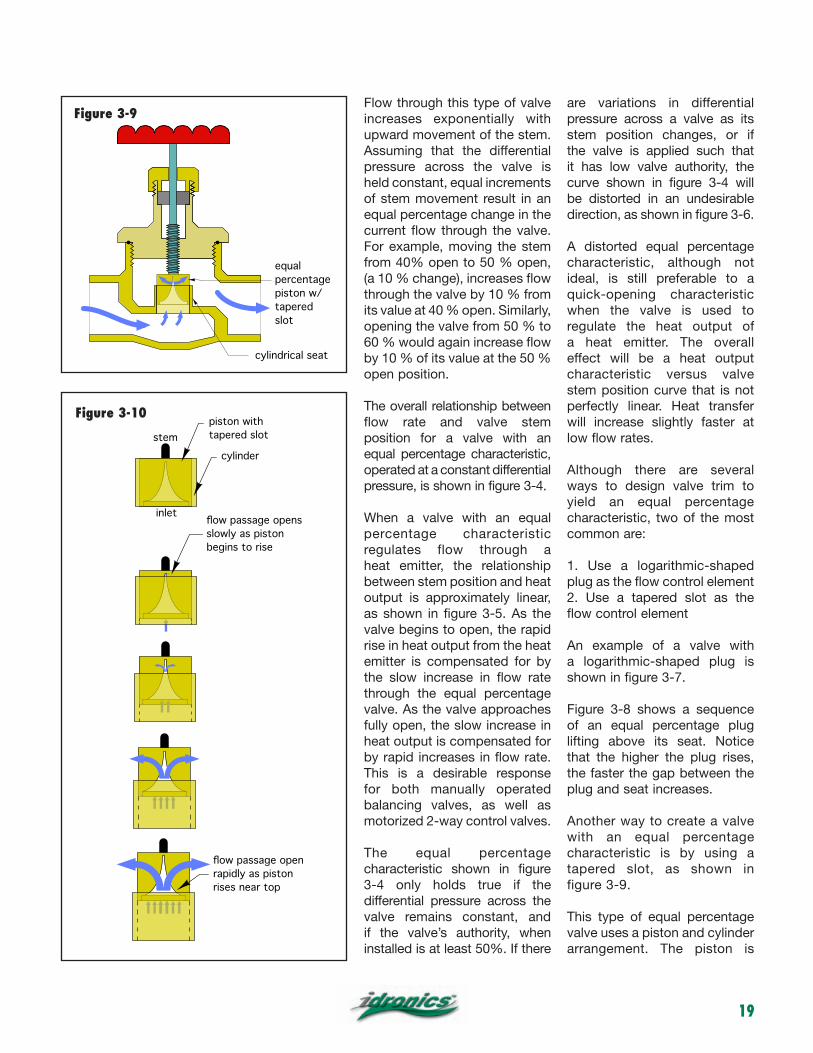
Another way to create a valve with an equal percentage characteristic is by using a tapered slot, as shown in figure 3-9.

This type of equal percentage valve uses a piston and cylinder arrangement. The piston is

stempiston with !tapered slot

cylinder

flow passage opens!slowly as piston!begins to rise

inlet

flow passage open!rapidly as piston!rises near top

equal !percentage !piston w/!tapered!slot!

cylindrical seat

Figure 3-9

Figure 3-10

20

open at the bottom and contains one or two tapered slots along its side. As the piston is lifted through the cylinder, the narrow end of the tapered slot rises above the upper edge of the cylindrical seat, allowing a small flow to pass through. The higher the piston rises above the cylinder, the faster the open flow passage area of the tapered slot increases. This allows the flow rate to increase exponentially as the piston rises. Figure 3-10 shows a sequence of an equal percentage piston with tapered slot lifting above its cylindrical seat.

Valves with tapered slots are also used for the valves in some manifolds, as seen in figure 3-11.

Another difference between a standard flat-disc globe valve, and an equal percentage valve is the pitch of the threads that determine the linear shaft movement per turn of the shaft. A standard globe valve usually requires 3 to 4 turns of its shaft to move its disc from the fully closed to the fully open position. Most equal percentage balance valves require 5 to 10 turns for the same linear movement. This allows more precise setting of the flow control plug, and thus provides better control of flow rate.

DIFFERENTIAL PRESSURE TYPE BALANCING VALVES:Neither a globe valve, nor a basic valve with equal percentage trim indicate the flow rate passing through them. Knowing this flow rate greatly assists in properly setting the balancing valve.

One type of valve that addresses the need to know flow rate is shown in figure 3-12. It is known as a differential pressure type balancing valve.

This valve has two additional ports cast and machined into its body; one on the upstream side of the valve seat, and the other on the downstream side. When a differential pressure measuring device is attached across these ports, it is possible to read the pressure drop across the valve’s seat. The flow rate through the valve can then be read from a chart, slide rule or calculated with another device based on a previously determined precise relationship between differential pressure and flow rate.

Another variation on this valve uses pressure ports on both the inlet and throat (vena contracta) of a venturi flow passage, as seen in figure 3-13. The venturi passage maintains a very stable relationship between differential pressure and flow rate, more stable than that of valves that measure differential pressure across the flow plug. A separate flow control element (plug or tapered slot) is located downstream of the venturi passage and pressure tappings.

tapered slot!for equal percentage!characteristic

Figure 3-11

Figure 3-12

Figure 3-13

21

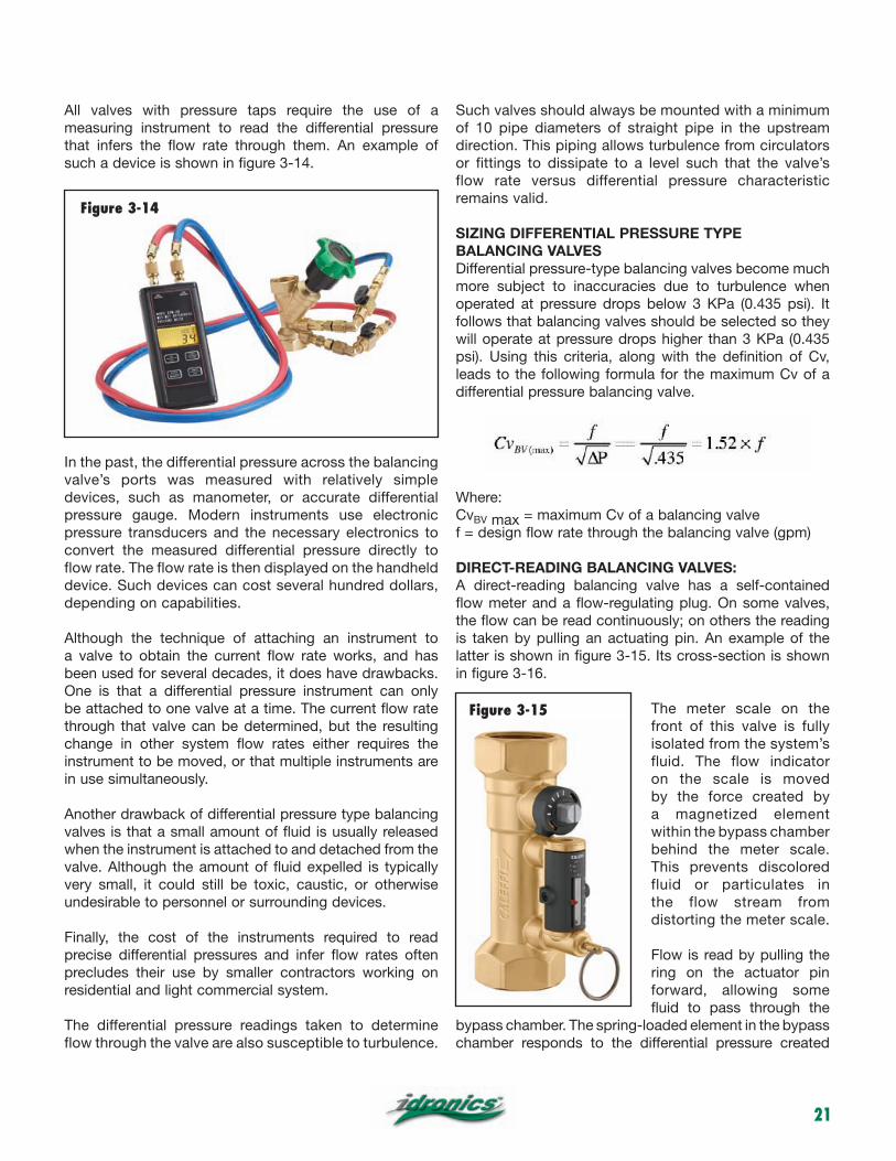
All valves with pressure taps require the use of a measuring instrument to read the differential pressure that infers the flow rate through them. An example of such a device is shown in figure 3-14.

In the past, the differential pressure across the balancing valve’s ports was measured with relatively simple devices, such as manometer, or accurate differential pressure gauge. Modern instruments use electronic pressure transducers and the necessary electronics to convert the measured differential pressure directly to flow rate. The flow rate is then displayed on the handheld device. Such devices can cost several hundred dollars, depending on capabilities.

Although the technique of attaching an instrument to a valve to obtain the current flow rate works, and has been used for several decades, it does have drawbacks. One is that a differential pressure instrument can only be attached to one valve at a time. The current flow rate through that valve can be determined, but the resulting change in other system flow rates either requires the instrument to be moved, or that multiple instruments are in use simultaneously.

Another drawback of differential pressure type balancing valves is that a small amount of fluid is usually released when the instrument is attached to and detached from the valve. Although the amount of fluid expelled is typically very small, it could still be toxic, caustic, or otherwise undesirable to personnel or surrounding devices.

Finally, the cost of the instruments required to read precise differential pressures and infer flow rates often precludes their use by smaller contractors working on residential and light commercial system.

The differential pressure readings taken to determine flow through the valve are also susceptible to turbulence.

Such valves should always be mounted with a minimum of 10 pipe diameters of straight pipe in the upstream direction. This piping allows turbulence from circulators or fittings to dissipate to a level such that the valve’s flow rate versus differential pressure characteristic remains valid.

SIZING DIFFERENTIAL PRESSURE TYPE BALANCING VALVESDifferential pressure-type balancing valves become much more subject to inaccuracies due to turbulence when operated at pressure drops below 3 KPa (0.435 psi). It follows that balancing valves should be selected so they will operate at pressure drops higher than 3 KPa (0.435 psi). Using this criteria, along with the definition of Cv, leads to the following formula for the maximum Cv of a differential pressure balancing valve.

Where:CvBV max = maximum Cv of a balancing valvef = design flow rate through the balancing valve (gpm)

DIRECT-READING BALANCING VALVES:A direct-reading balancing valve has a self-contained flow meter and a flow-regulating plug. On some valves, the flow can be read continuously; on others the reading is taken by pulling an actuating pin. An example of the latter is shown in figure 3-15. Its cross-section is shown in figure 3-16.

The meter scale on the front of this valve is fully isolated from the system’s fluid. The flow indicator on the scale is moved by the force created by a magnetized element within the bypass chamber behind the meter scale. This prevents discolored fluid or particulates in the flow stream from distorting the meter scale.

Flow is read by pulling the ring on the actuator pin forward, allowing some fluid to pass through the

bypass chamber. The spring-loaded element in the bypass chamber responds to the differential pressure created

Figure 3-14

Figure 3-15

22

across the precision orifice in the main flow passage. As the spring-loaded assembly moves, magnetic forces move the indicator on the meter scale. When the ring is released, flow through the bypass chamber stops.

This valve, which can be mounted in any position, also allows adjustment of flow rate by turning the stem located above the flow meter.

Metered balancing valves are also available on some manifold systems, as shown in figure 3-17. In most cases, the flow indicated is spring-loaded, allowing the manifold to be mounted in any orientation. Flow adjustments to each circuit are made by rotating the flow indicator column, which is directly connected to the shaft of the internal valve.

PRESSURE-INDEPENDENT BALANCING VALVES (PIBV):Section 2 described the fact that adjusting the flow rate in any crossover of a multi-crossover hydronic system causes the flow rates in other crossovers to change. This will always be the case when a “static,” or “manually set” balancing valve is used.

A more recent development in hydronic balancing is called a pressure-independent balancing valve (PIBV). These valves are configured to maintain a preset flow rate over a wide range of differential pressure. They rely on an internal compensating mechanism to adjust a flow orifice within the valve so that a calibrated flow rate is maintained, typically within a tolerance of +/- 5 % of the flow rating. Figure 3-18a shows one body style used for PIBVs. The internal components in a pressure-independent balancing valve consist of a cylinder, a spring-loaded piston, and a combination of fixed and variable shape orifices through which flow passes. The assembly of these components is called the “cartridge” of the PIBV. An example of such a cartridge is seen in figure 3-18b.

Pressure-independent balancing valves are also available in the Y-pattern body style shown in figure 3-19a. A cross-section of this style of PIBV is shown in figure 3-19b.

The Y-pattern PIBV uses the same flow control cartridges as the inline style PIBV shown in figure 3-18a. However, in addition to the flow control cartridge, the Y-pattern valve includes a ball valve for flow isolation, the option of attaching a drain valve to the lower port for reverse flushing the cartridge, and pressure tap ports on either side of the flow cartridge. The latter can be used to verify flow rate through the PIBV during system commissioning.

At low differential pressures, (less than 2, 4, or 5 psi, depending on valve model), the internal compensating mechanism does not move. This allows the maximum free flow passage through the valve. Flow passes through both the fixed and variable orifices. However, at such low differential pressures, the internal mechanism cannot adjust to maintain a fixed

Figure 3-16

Figure 3-17

23

flow rates. Thus, flow rate through the valve will increase as differential pressure increases. The “inactive” position of the internal cartridge is shown in figure 3-20.

If the differential pressure across the PIBV exceeds the minimum threshold pressure of 2, 4, or 5 psi (depending on valve model), the internal piston assembly begins to move in the direction of flow due to thrust against it. An internal spring is partially compressed by this action. Under this condition, the piston partially obstructs the tapered slot through which flow must pass. However, the flow passage is now automatically adjusted so that the valve can maintain its calibrated flow rate at the higher differential pressure.

If the differential pressure across the valve continues to increase, the piston moves farther, and further compresses the spring. This movement continues to reduce the flow passage through the tapered orifice, as seen in figure 3-21. The change in the orifice size is such that the valve continues to deliver its calibrated flow rate under the higher differential pressure.

cartridge

fixed orificetapered (variable) orifice

pistonspring

body

Figure 3-18a Figure 3-18b

Figure 3-19a Figure 3-19b

Figure 3-20

24

This ability to adjust flow through the tapered orifice remains in effect until the differential pressure across the valve exceeds an upper threshold limit of 14, 32, 34, or 35 psi (depending on valve model). Such high differential pressure is relatively uncommon in most well-designed hydronic systems that include some means of differential pressure control.

If the differential pressure across the valve does exceed the upper pressure threshold, the piston and counterbalancing spring can no longer maintain the calibrated flow rate. The piston’s position completely blocks flow through the tapered orifice. All flow must now pass through the fixed orifice. This condition is shown in figure 3-22. The result will be an increase in flow rate if differential pressure increases above the upper pressure threshold.

The unique polymer cartridges used in all Caleffi PIBVs are specifically designed for low flow noise.

The overall flow versus differential pressure characteristics of a PIBV is shown in figure 3-23. The desired condition is to maintain the differential pressure across the valve between the lower and upper threshold values, so that the internal cartridge remains active, and the valve maintains its rated flow rate.

With a PIBV in each crossover, the flow rates through each active crossover remains at its design value, regardless of the flow status in other crossovers. However, this desirable condition is contingent upon keeping the differential pressure across the PIBV between its lower and upper threshold values. This condition is vitally important to proper application of such valves, and will be discussed further in section 5.

Figure 3-24 compares the flow rate changes in two identical systems, with the exception of the type of balancing valve used.

The system in figure 3-24a uses manually set “static” balancing valves that have been adjusted so that the desired flow rates exist in each crossover, provided all crossovers are active. However, when a zone valve in one of the crossovers closes, the flow rates in the other crossovers increase due to the increased differential pressure created by the fixed-speed circulator. This change in flow rates is undesirable because it increases heat output from the heat emitters.

flow rate

diffe

rent

ial p

ress

ure

2 psi

32 psipressure drop curve of PIBV when spring!is fully compressed

pressure drop curve of PIBV when spring!is fully extended

desireable working!range of

PIBV

rated flow rate of PIBV

Figure 3-21

Figure 3-22

Figure 3-23

25

VENT

ONheat emitter

supp

ly m

ain

retu

rn m

ain

6 gpm

4 gpm

8 gpm

4 gpm

fixed speed

circulator

zone valve

ON

ON

ON

"static" balancing valve

22 gpm

VENT

ON

supp

ly m

ain

retu

rn m

ain

6.2 gpm

4.5 gpm

0 gpm

4.6 gpm

fixed speed

circulator

ON

OFF

ON

15.3 gpm

flow rate (gpm)

0

2

4

6

8

10

12

14

16

18

0 2 4 6 8 10 12 14 16 18 20 22 24 26 28 30 32 34 36 38 40

pump curve

head

add

ed o

r los

t (fe

et)

system head loss curve (4 zones on)system head loss curve (3 zones on)

increased!differential!pressure

∆P = ∆HD

144⎞⎠⎟⎜

⎛⎝

VENT

ONheat emitter

supp

ly m

ain

retu

rn m

ain

6 gpm

4 gpm

8 gpm

4 gpm

fixed speed

circulator

zone valve

ON

ON

ON

"static" balancing valve

22 gpm

VENT

ON

supp

ly m

ain

retu

rn m

ain

6.2 gpm

4.5 gpm

0 gpm

4.6 gpm

fixed speed

circulator

ON

OFF

ON

15.3 gpm

flow rate (gpm)

0

2

4

6

8

10

12

14

16

18

0 2 4 6 8 10 12 14 16 18 20 22 24 26 28 30 32 34 36 38 40

pump curve

head

add

ed o

r los

t (fe

et)

system head loss curve (4 zones on)system head loss curve (3 zones on)

increased!differential!pressure

∆P = ∆HD

144⎞⎠⎟⎜

⎛⎝

Figure 3-24a

26

VENT

ON

heat emitter

supp

ly m

ain

retu

rn m

ain

6 gpm

4 gpm

8 gpm

4 gpm

fixed speed

circulator

zone valve

ON

ON

ON

pressure independent!balancing valve

22 gpm

VENT

ONsu

pply

mai

n

retu

rn m

ain

0 gpm

fixed speed

circulator

ON

OFF

ON

14 gpm

6 gpm

4 gpm

4 gpm

No change in flow rates within zones

that remain on

flow rate (gpm)

0

2

4

6

8

10

12

14

16

18

0 2 4 6 8 10 12 14 16 18 20 22 24 26 28 30 32 34 36 38 40

pump curve

head

add

ed o

r los

t (fe

et)

system head loss curve (4 zones on)

system head loss curve !(3 zones on)

increased!differential!pressure

∆P = ∆HD

144⎞⎠⎟⎜

⎛⎝

minimum ∆P threshold for!pressure-independent valves

Figure 3-24b

VENT

ON

heat emitter

supp

ly m

ain

retu

rn m

ain

6 gpm

4 gpm

8 gpm

4 gpm

fixed speed

circulator

zone valve

ON

ON

ON

pressure independent!balancing valve

22 gpm

VENT

ON

supp

ly m

ain

retu

rn m

ain

0 gpm

fixed speed

circulator

ON

OFF

ON

14 gpm

6 gpm

4 gpm

4 gpm

No change in flow rates within zones

that remain on

flow rate (gpm)

0

2

4

6

8

10

12

14

16

18

0 2 4 6 8 10 12 14 16 18 20 22 24 26 28 30 32 34 36 38 40

pump curve

head

add

ed o

r los

t (fe

et)

system head loss curve (4 zones on)

system head loss curve !(3 zones on)

increased!differential!pressure

∆P = ∆HD

144⎞⎠⎟⎜

⎛⎝

minimum ∆P threshold for!pressure-independent valves

27

The system in figure 3-24b uses PIBVs in each crossover. Each valve has been configured with a flow cartridge for the design flow rate of its crossover. When one of the zone valves closes, the PIBVs in the other crossovers immediately compensate for the increased differential pressure so that the flow through each active crossover remains the same.

The cartridges within each active PIBV absorb the increased head energy from the circulator when the operating point moves to the left and up on the pump curve.

PIBVs are often used to control flow rates through air handlers or water-source heat pumps. Figure 3-25 shows a typical piping configuration for an air handler. In the case of heat pumps, pressure-rated, flexible hose connections are often used to transition from the piping

connections on the heat pump to the rigid piping. These hoses dampen vibration transmission and allow more flexibility in the piping layout near the heat pump.

The Y-strainer is placed on the inlet piping to the air handler to capture any dirt particles carried along by the flow stream before they enter the other components. The differential pressure across the Y-strainer increases as dirt particles accumulate, and it is monitored using the pressure gauges. When necessary, the Y-strainer can be isolated and opened to clean its internal screen. The PIBV maintains a fixed flow rate through the air handler’s coil whenever the zone valve is open, and the differential pressure between the supply and return piping connections is within the regulating range of the flow cartridge in the PIBV.

air handler

zone valve#120 Y-strainer!w/ isolation valve

#121 FLOWCAL!w/ isolation valve

Figure 3-25

28

4. BALANCING PROCEDURES FOR SYSTEMS USING MANUALLY SET BALANCING VALVES

This section discusses procedures for balancing typical hydronic systems using manually set balancing valves. These include the differential pressure-type balancing valves and direct-reading balancing valves discussed in the previous section.

The ultimate goal of balancing a hydronic system is achieving the correct rate of heat delivery to each space served by the system. This goal relies on the assumption that the load for each space has been predetermined through accurate load calculations, and that the building is constructed so that its heat losses exactly match those load calculations.

Using these calculated load values, and a selected temperature drop for each heat emitter, the necessary flow rate through each portion of the system is calculated. The balancing procedure is then used to establish those flow rates throughout the system.

Establishing a set of predetermined flow rates is the “customary” outcome of the balancing procedures discussed in this section. Keep in mind, however, that establishing a set of calculated flow rates does not guarantee that the desired heat transfer occurs at all heat emitters. The latter can only be done, on a theoretical basis, through simulations that simultaneously account for the both the thermal and hydraulic characteristics of all portions of the system. Even the results of these simulations are only as valid as the accuracy of the load calculations.

return main

supply main

circ

ulat

or

heat input

cros

sove

r

balancing valves

return main

supply main

circ

ulat

or

least favored branch

heat input

most favored branch

Figure 4-1

Figure 4-2

29

Although balancing to establish a set of predetermined flow rates is not guaranteed to produce perfect comfort in all spaces, it certainly is a means toward that end, and thus an essential part of modern hydronics technology.

BALANCING BASICS:Consider the hydronic distribution system shown in figure 4-1.

It consists of nine crossovers connected across common supply- and return mains. Circulation is created by a fixed-speed circulator. This piping arrangement is called a parallel direct return system. For simplicity, assume that all crossovers have identical piping components, and thus should (ideally) all operate at the same flow rate and head loss. The vertical piping near the circulator, and the closely spaced tees where heat is added, can be considered to have insignificant head loss.

Assume that when this system is first turned on, all the balancing valves are fully open. Because of the head loss along the supply main and return main, the differential pressure exerted across each crossover will be different.

The “most favored crossover” nearest the circulator will have the highest differential pressure and thus the highest flow rate. The “least favored crossover” at the far right side of the system will have the lowest differential pressure and thus the lowest flow rate. This undesirable but none-the-less present condition, shown in figure 4-2, is what proper balancing is meant to correct.

Figure 4-3 is a graphic representation of how head energy is added to the system by the circulator and is dissipated as flow passes along the supply and return mains and through the crossovers.

The vertical line to the left of the circulator represents the head required to push flow along the supply header, through the least favored crossover at the design flow rate, and back through the return main.

The sloping lines above and below the piping represent head being dissipated as flow moves through the supply and return mains. These lines get closer to each other as they progress from left to right. This implies that each crossover has less head available to it than the crossover to its left, due to head dissipation in each segment of

return main

Hcirc

ulat

or

head loss along supply main

Hbra

nch

head loss along supply main

supply main

heat input

balancing valves

"overflow" in all crossovers other than !the one farthest from the circulator

desired flow rate

Figure 4-3

30

supply main

return main

Hcirc

ulat

or

equal head loss across each crossover!(creating equal flow through each crossover)

Hbra

nch

(leas

t fa

vore

d)

head dissipated by each balancing valve

Hbra

nch

(leas

t fa

vore

d)Hb

alan

cing

val

veheat input

Hexcess

supply main

return main

Hcirc

ulat

or

Hbra

nch

(leas

t fa

vore

d)

head dissipated by each balancing valve

Hbra

nch

(leas

t fa

vore

d)Hb

alan

cing

val

ve

heat input

equal head loss across each crossover!(creating equal flow through each crossover)

Figure 4-4

Figure 4-5

31

the mains. Less available head means lower differential pressure across the crossover, and thus lower flow rate.The head available to the “least favored crossover” at the far right of the system determines the flow rate through the crossover. In this system, the circulator is assumed to be sized so that it can provide the necessary head to drive flow through the least favored crossover, accounting for the head loss along the full length of the supply and return mains.

This initial unbalanced conditions leads to “overflow” in all crossovers other than the least favored crossover, as indicated by the flow arrows. Such overflow increases the wattage demand of the circulator, and thus increases the operating cost of the system. Overflow may also result in unacceptable flow noise and/or erosion corrosion of copper fittings.

To achieve equal flow in each crossover, there must be an equal head loss (and thus an equal differential pressure) across each crossover. This requires the balancing valve in each crossover to dissipate the difference between the head available between the supply and return mains, and the head dissipated by the other piping components in the crossover. This concept is shown in figure 4-4.

The head that each balancing valve must dissipate is indicated by the vertical height of the yellow shaded area at each crossover location. In this system, which assumes identical crossover piping and mains piping that is sized for a consistent head loss per unit of length, the required head dissipation of each balancing valve is proportionally less than that of the balancing valve to its left. The balancing valve on the most favored crossover (at left) needs to dissipate the greatest head, while the balancing valve on the least favored crossover (at right) needs to dissipate zero head. The latter case assumes that the circulator is sized to provide exactly the head required by flow along the full length of the mains and through the least favored crossover. If the circulator supplies excess head, the balancing valve in the least favored circuit will also have to be partially closed to absorb some excess this head, as shown in figure 4-5.

In some systems, the hydraulic resistance of a given crossover may be significantly different from the others. The design flow rate requirement may also vary from one crossover to another. It is still possible to balance such systems for the desired flow rate in each crossover. In each case, a properly adjusted balancing valve will absorb the difference between head available across the mains at the location of the crossover, and the head required to sustain the design flow rate through the crossover. This concept is shown in figure 4-6.

DETERMINING CROSSOVER FLOW RATES:The first step in balancing a system is determining the “target” flow rate through each crossover under design load conditions. These flow rates are typically found using Formula 4-1:

Hbal

anci

ng v

alve

1

Hcirc

ulat

or

Hcro

ssov

er 1

BV1

BV2

BV3

Hbal

anci

ng v

alve

2

Hbal

anci

ng v

alve

3

Hcro

ssov

er 2

Hcro

ssov

er 3

slope is due to !head loss along !supply main

supply main

return main

slope is due to !head loss along !return main

Figure 4-6

Formula 4-1

32

Where: fi = target flow rate in crossover “i” (where i is any crossover number from 1 to the total number of crossovers)Qi = design heating load required of the crossover (Btu/hr)D = density of the fluid at the average system operating temperature (lb/ft3)c = specific heat of the fluid at the average system operating temperature (Btu/lb/ºF)∆Td = temperature drop assumed under design load conditions (ºF)8.01 = a constant based on the units in the formula.

The value of the grouping (8.01Dc) can be read from figure 4-7, based on three selected average system fluid temperatures, and three different fluids.

Example: Assume a crossover is to deliver 50,000 Btu/hr of heating at design load conditions. The system operates with water being supplied at 170 ºF and a target temperature drop, under design load conditions, of 20 ºF. Determine the target flow rate for the crossover.

Solution: The average water temperature at design load will be the supply temperature minus half the temperature drop:

Since figure 4-7 has no value for the quantity (8.01Dc) listed at 160 ºF, it is necessary to interpolate between the values given at 140ºF and 180 ºF. In this case it is a simple average:

The target flow rate can now be calculated from Formula 4-1:

This calculation would be repeated for each crossover in the system.

Once the design load flow rates for each crossover are determined, they can be added as necessary to determine the flow rates through the various segments of the supply and return mains.

BALANCING USING PRESET METHOD:One method of balancing a hydronic system is called the “preset method.” It calculates the necessary Cv of each balancing valve based on the design load flow rate required through each crossover, and each crossover’s location within the system.

Consider the typical crossover piping shown in figure 4-8.

The total head loss from the supply main to the return main consists of the head loss across the piping, fittings, heat emitter, and zone valve, plus the head loss across the balancing valve. For simplicity, the head loss of the piping, fittings, heat emitter and zone valve are combined into one quantity called ∆Hpiping+HE. Thus:

zone valve

heat emitterbalancing

valve

supp

ly m

ain

retu

rn m

ain

∆Hmains

∆Hpiping+HE ∆HBV

∆Hcirculator

L

supply main

return main

∆Hmains ∆Hcirculator 2L(.04)-=

insig

nific

ant

head

loss

Figure 4-7

Figure 4-8

Figure 4-9

33

To achieve the desired flow rate across this crossover, the balancing valve must absorb the difference between ∆Hmains and ∆Hpiping+HE:

The necessary Cv setting for the balancing valve can be found using Formula 4-4.

To evaluate Formula 4-4, it is necessary to know the head loss across the mains at the location of the crossover, as well as the head loss of the piping and heat emitter in that crossover when operating at design flow rate.

The head loss of the piping and heat emitter at design flow rate should be determined through standard hydronic design calculations based on the specific heat emitter selected, the piping type, size and length, the fittings, and the zone valve used in the crossover. The head loss of all these components should be determined at the design flow rate of the crossover. Methods for calculating such head losses are given in Appendix B.

The total head loss along the mains is harder to determine. It will depend on the type, size and length of tubing in each segment of the supply and return mains, as well as the flow rates present within each segment.

One method of approximating the drop in head across the mains is to assume that the mains are sized based on a specific head loss per foot. A common range for such head loss is 3 to 5 feet of head loss per 100 feet of pipe. Sizing the mains for the lower end of this range will reduce the total head across the circulator, at the expense of slightly larger piping. Sizing for the upper end of the range will likely decrease the size of the mains piping, but at the expense of greater circulator head, and thus higher operating cost over the life of the system.

VENT

retu

rn m

ain

load = 49,000 Btu/hr

50 ft

75 ft

branch #3

branch #2

branch #1

load = 98,000 Btu/hr

load = 29,400 Btu/hr90 ft

mains piping sized for

head loss of 4 ft per 100

feet

flow rate (gpm)

0

2

4

6

8

10

12

14

16

18

0 2 4 6 8 10 12 14 16 18 20 22 24 26 28 30

head

add

ed (f

eet)

pump curve of installed circulator

Figure 4-10a

Figure 4-10b

34

For our discussions, we will assume that the supply and return mains will be consistently sized for a nominal 4 feet of head loss per hundred feet of pipe. Using this assumption, the head loss across the mains at some location downstream of the circulator can be estimated as shown in figure 4-9.

The hydraulic separator in figure 4-9 is where heat is added to the distribution system, and it represents insignificant head loss. The head loss of the supply and return mains is estimated by subtracting an assumed 4 feet of head loss per hundred feet of mains piping from the head produced by the circulator. This relationship is given as formula 4-5.

Where:∆Hmains = head loss between supply and return main (feet of head)∆Hcirculator = circulator head at design flow rate (feet of head)L = length of supply or return main from heat source out to the crossover (feet)0.04 = assumed head loss of 4 feet per 100 feet of main piping

Example: The system shown in figure 4-10a requires balancing. The system is operating with water at an average temperature of 140ºF. The design load temperature drop assumed for each crossover is 20ºF. The required design heating load of each crossover is indicated. The supply and return main piping has been sized for a head loss of 4 feet per 100 feet. The circulator used in the system has the pump curve shown in figure 4-10b Determine:

a. The required design flow rate in each crossoverb. The required Cv setting of the balancing valve in each crossover

Solution: The required design load flow in each crossover is determined using Formula 4-1. The value of (8.01Dc) for water at an average temperature of 140 ºF is 490.

For crossover #1:

For crossover #2:

For crossover #3:

Using these flow rates, the head loss of the piping components and heat emitter in each crossover (exclusive of the balancing valve) are determined using standard head loss calculation methods (see Appendix B). The values that we will assume as the result of these calculations are shown in figure 4-11.

The total of the three crossover flow rates, 18 gpm, is the required system flow rate. The pump curve of the selected circulator indicates it adds 12 feet of head to the water at this flow rate.

The head loss across the mains at each crossover location is now calculated using Formula 4-5:

For crossover #1:

For crossover #2:

For crossover #3:

The required head loss across each balancing valve can now be calculated using Formula 4-3:

For crossover #1:

For crossover #2:

For crossover #3:

Figure 4-11

larger piping. Sizing for the upper end of the range will likely decrease the size of the mains piping, but at the expense of greater circulator head, and thus higher operating cost over the life of the system.

For our discussions, we will assume that the supply and return mains will be consistently sized for a nominal 4 feet of head loss per hundred feet of pipe. Using this assumption, the head loss across the mains at some location downstream of the circulator can be estimated as shown in figure 4-9.

[insert figure 4-9]

∆Hcirculator

L

supply main

return main

∆Hmains ∆Hcirculator 2L(.04)-=

insig

nific

ant

head

loss

The hydraulic separator in figure 4-9 is where heat is added to the distribution system, and it represents insignificant head loss. The head loss of the supply and return mains is estimated by subtracting an assumed 4 feet of head loss per hundred feet of mains piping from the head produced by the circulator. This relationship is given as formula 4-5.

Formula 4-5

Where:∆Hmains = head loss between supply and return main (feet of head)∆Hcirculator = circulator head at design flow rate (feet of head)L = length of supply or return main from heat source out to the crossover (feet)0.04 = assumed head loss of 4 feet per 100 feet of main piping

Example: The system shown in figure 4-10a requires balancing. The system is operating with water at an average temperature of 140ºF. The design load temperature drop assumed for each crossover is 20ºF. The required design heating load of each crossover is indicated. The supply and return main piping has been sized for a head loss of 4 feet per 100 feet. The circulator used in the system has the pump curve shown in figure 4-10b Determine:

a. The required design flow rate in each crossover

Formula 4-5

35

VENT

retu

rn m

ain

differential pressure !bypass valve!

(set for 12.5 to 13 ft)!(5.3 to 5.5 psi)

branch #3

branch #2

branch #1

supp

ly m

ain

flow rate (gpm)

0

2

4

6

8

10

12

14

16

18

0 2 4 6 8 10 12 14 16 18 20 22 24

head

add

ed (f

eet)

"effective" pump curve when DPBV is operating

1.0

2.0

3.0

4.0

5.0

6.0

0

diffe

rent

ial p

ress

ure

acro

ss m

ains

(psi

)

threshold setting of DPBV (5.5 psi)

operating point with all zones open

representation of system head loss curve!with 1 zone closedrepresentation of system head loss curve!with 1 zone closed

representation of system head loss curve!with 2 zones closedrepresentation of system head loss curve!with 2 zones closed

The required Cv of each balancing valve can now be calculated using Formula 4-3:

For crossover #1:

For crossover #2:

For crossover #3:

The balancing valve in each crossover can now be set to the required Cv values using a scale built into the valve’s stem, or using a graph / table indicating Cv versus stem position. An example of the latter is shown in figure 4-12.

Discussion: This procedure is based on an estimate of head loss in the mains. As such it is not guaranteed to yield the exact design flow rates when the balancing valves are set to the calculated Cv values. If metered balancing valves are used, each crossover flow rate can be “fine-tuned” to the required value.

Figure 4-12

Figure 4-13

36

Finally, there is no differential pressure bypass valve (DPBV) shown in the system of figure 4-10a. This will result in some fluctuation of zone flow when one or more of the zone valves closes. To reduce this variation, a DPBV can be installed as shown in figure 4-13, and set for (5.5 psi). This is just slightly above the 12-foot head produced by the circulator at design flow rate. This setting allows the DPBV to remain

terminal!unit #1

terminal!unit #2

terminal!unit #3

terminal!unit #4

BV2BV3BV4 BV1

partner valve

heating or

cooling plant

terminal!unit #1

terminal!unit #2

terminal!unit #3

terminal!unit #4

terminal!unit #1

terminal!unit #2

terminal!unit #3

terminal!unit #4

terminal!unit #1

terminal!unit #2

terminal!unit #3

terminal!unit #5

branch #1

risers

BV2BV3BV4 BV1

partner valve #1

branch #2

branch #3

partner valve #2

partner valve #1

BV4 BV2BV3 BV1BV5

BV2BV3 BV1

riser!balancing!valve

heating or

cooling plant

terminal!unit #1

terminal!unit #2

terminal!unit #3

terminal!unit #4

terminal!unit #1

terminal!unit #2

terminal!unit #3

terminal!unit #4

terminal!unit #1

terminal!unit #2

terminal!unit #3

terminal!unit #5

branch #1

riser!set #1

BV2BV3BV4 BV1

partner valve #1

branch #2

branch #3

partner valve #2

partner valve #1

BV4 BV2BV3 BV1BV5

BV2BV3 BV1

riser!balancing!valve #1

terminal!unit #1

terminal!unit #2

terminal!unit #3

terminal!unit #4

terminal!unit #1

terminal!unit #2

terminal!unit #3

terminal!unit #4

terminal!unit #1

terminal!unit #2

terminal!unit #3

terminal!unit #5

branch #1

BV2BV3BV4 BV1

partner valve #1

branch #2

branch #3

partner valve #2

partner valve #1

BV4 BV2BV3 BV1BV5

BV2BV3 BV1

riser!balancing!valve #2

riser!set #2

building main!balancing!

valve

building mains

heating or

cooling plant

Figure 4-14

Figure 4-15 Figure 4-16

37

closed under design load conditions when all zones are operating. When one or more zone valves close, the differential pressure between the mains will increase slightly, and some flow will now pass through the DPBV, which will stabilize the differential pressure between the supply and return mains. The flow rate in the zones that are on will remain relatively stable; however, a slight increase in flow rate should be expected through these zones because the pressure drop along the mains will be less due to reduced flow.

BALANCING USING COMPENSATED METHODAnother method for balancing systems that use differential pressure-type balancing valves is called the “compensated method.” It can be used in relatively simple systems, such as shown in figure 4-14, or in systems with multiple branches connected to a set of risers, as shown in figure 4-15. It can even be used in systems that have multiple sets of risers connected to a common set of building mains, as shown in figure 4-16.

Figures 4-14, 4-15, and 4-16 all show “terminal units” as part of the piping system. A terminal unit is any device used for delivering heating or cooling. Examples of terminal units include radiators, fan-coils, manifold stations serving radiant panel circuits, or finned-tube convectors. In the case of a heating-only system, the term terminal unit is synonymous with heat emitter.

A heating or cooling “plant” refers to any device or group of devices that produce heated or chilled water.

The discussions in this section further assume that the heating or cooling plant is hydraulically separated from the distribution system. This prevents flow rate changes within the distribution system from inherently altering flow rates in the heating or cooling plant. There are several ways to achieve this hydraulic separation. They include use of a hydraulic separator, closely spaced tees, or a buffer tank. These methods are shown in figure 4-17.

VENT

hydraulic separator

boiler !system

controller

boiler #1 boiler #2

to / from!distribution!

system

VENT

closely!spaced!tees

boiler !system

controller

boiler #1 boiler #2

to / from!distribution!

system

VENT

boiler !system

controller

boiler #1 boiler #2

to / from!distribution!

system

buffer!tank

Figure 4-17

38

As system piping becomes more complex, it is important to establish consistent terminology. Terms such as “branch,” “riser,” “mains,” “crossover,” or “header” can mean different things to different people. For discussing these systems, the terminology shown and identified in figure 4-18 will be used.

The compensated method of balancing divides the overall system task into subsystems. It sequentially applies the balancing process from smaller to larger subsystems. The sequence used is as follows:

terminal!unit #1

terminal!unit #2

terminal!unit #3

terminal!unit #4

terminal!unit #1

terminal!unit #2

terminal!unit #3

terminal!unit #5

branch #1

riser!set #1

partner valve #1

branch #2

branch #3

partner valve #2

partner valve #1

BV4 BV2BV3 BV1BV5

BV2BV3 BV1

riser!balancing!valve #1

heating or

cooling plant

riser!set #2

riser!set #3

building main!balancing!

valve

building mains

crossover

terminal!unit #1

terminal!unit #2

terminal!unit #3

terminal!unit #4

BV4 BV2BV3 BV1

terminal!unit #1

terminal!unit #2

terminal!unit #3

terminal!unit #4

BV2BV3BV4

reference valve

least favored!

crossover

∆P

partner valve

branch

#1#1#2#3#4

Figure 4-18

Figure 4-19

39

1. A given branch of the system is selected, and the individual crossovers within that branch are balanced relative to each other.

2. Each branch on a riser set is then balanced relative to the other branches on that riser set.

3. If the system contains multiple riser sets, each riser set is then balanced relative to each other.

The compensated method assumes the design flow rates through each portion of the system have been predetermined through calculations, such as those described earlier in this section.

The compensated balancing method, when used with differential pressure balancing valves, required at least one, and preferably two, differential pressure meters that can accurately display the differential pressure across any balancing valve they are attached to.

In most cases this method of balancing is best performed by two technicians working as a team. The two technicians will often be in different locations within the building where specific balancing valves are located, and they will need to stay in communication with each other as the balancing procedure progresses.

The system should be fully purged and all balancing valves set to their fully open position before beginning the balancing process.

If there are multiple riser sets in the system, select the riser set farthest from the circulator, and temporarily shut off flow to the other riser sets. Since a riser must have at least two branches, select the branch farthest from the circulator. The balancing valves on all crossovers with this branch will be adjusted before moving to a different branch.

Consider the branch shown in figure 4-19. It consists of 4 crossovers, each serving a terminal unit, and each containing a differential pressure-type balancing valve. Another balancing valve, known as the “partner valve” is located on the return pipe of the branch.

The following procedure can be used to adjust the balancing valves in this branch.

Step 1: Identify the “least favored crossover” within the branch. If the terminal units are similar or identical, the least favored crossover will likely be that at the far end of the branch. If the crossovers have significantly different piping, the least favored crossover will be the one with the highest head loss at design flow conditions.

Identifying this crossover may require calculating the heat loss of each crossover in the branch. The balancing valve in the least favored crossover will now be called the “reference valve.”

Step 2: Set the reference valve for a minimum pressure drop that ensures stable and accurate readings. The commonly accepted value for this minimum pressure drop is approximately 3 KPa (0.435 psi). This minimizes the pressure drop (and head dissipation) across the balancing valve, while still maintaining the valve’s accuracy. If the Cv of this balancing valve was selected using the previously discussed formula:

The valve should be close to, or at, its fully open setting, and thus at its minimum head dissipation setting. Once this setting is made, lock the handwheel of the reference valve in this position. If the differential pressure across the valve cannot be set as low as 3 KPa (0.435 psi), leave the reference valve fully open.

Step 3: Attached a differential pressure meter to the reference valve as shown in figure 4-19.

Step 4: Adjust the partner valve on the branch return pipe so that the desired design flow rate is passing through the reference valve, and record the pressure drop across the reference valve. This pressure drop is now called the “reference pressure.”

Step 5: Move to the next crossover (#2 in figure 4-19). Adjust balancing valve BV2 so that the desired design flow rate is established through crossover #2. This will likely cause some change in the pressure drop read across the reference valve, which implies that the flow rate through crossover #1 has changed. This undesirable change will be corrected in the next step.

Step 6: Adjust the partner valve on the branch return pipe so that the pressure drop across the reference valve is restored to the reference pressure. This restores the design load flow rate across the reference valve. The flow rates in crossovers 1 and 2 are now proportionally balanced to each other. When one changes, the other will change proportionally. This is desirable.

Step 7: Move to the next crossover (#3 in figure 4-19). Adjust balancing valve BV3 so that the design flow rate is established through crossover #3. This will cause a change in the differential pressure read across the reference valve, which means there has been a change in flow rate.

40

Step 8: Again, adjust the partner valve so that the reference pressure is reestablished across the reference valve. This restores the design load differential pressure and flow rate. The flow rates in crossovers 1, 2, and 3 are now proportional to each other.

Step 9: Move to the next crossover (#4 in figure 4-19). Adjust balancing valve BV4 so that the desired design flow rate is established through this crossover. As before, this will likely cause some change in the pressure drop across the reference valve.

Step 10: Adjust the partner valve so that the reference pressure is reestablished across the reference valve. This restores the design load differential pressure and flow rate. The flow rates in crossovers 1, 2, 3 and 4 are now proportional to each other.

If there were more than 4 crossovers, this process would be repeated for each of the remaining crossovers. In each case, the desired design flow rate is established in a given crossover by adjusting its balancing valve. Any change in the reference pressure at the reference valve

terminal!unit #1

terminal!unit #2

terminal!unit #3

terminal!unit #4

terminal!unit #1

terminal!unit #2

terminal!unit #3

terminal!unit #4

terminal!unit #1

terminal!unit #2

terminal!unit #3

terminal!unit #5

branch #1

risers

BV2BV3BV4 BV1

partner valve #1

branch #2

branch #3

partner valve #2

partner valve #1

BV4 BV2BV3 BV1BV5

BV2BV3 BV1

riser!balancing!valve

heating or

cooling plant

branch #1

risers

partner valve #1

branch #2

partner valve #2

riser!partner!valve

branch #3

partner valve #2

reference valve

∆P

Figure 4-20

41

is then removed by adjusting the partner valve. When the balancing valves in all crossovers of the branch have been adjusted, all flow rates within those crossovers will change in proportion to each other, and the branch is considered “balanced.”

BALANCING MULTIPLE BRANCH SYSTEMS:After each branch attached to a riser set has been individually balanced using the above procedure, the same approach can be used to balance the branches relative to one another. Each branch can now be considered as if it were a single entity as shown in figure 4-20. None of the crossover balancing valves in any of the branches needs further adjustment.

The partner valve in the furthest branch becomes the new reference valve.

Step 1: Adjust the stem of the new reference valve (partner valve #1 in figure 4-20) so that it will create a minimum pressure drop of approximately 3 KPa (0.435 psi). Lock the handwheel of this valve at that setting. If the pressure drop cannot be lowered to 3 KPa, simply leave the valve in its fully open position.

Step 2: Connect the differential pressure meter across this valve, as shown in figure 4-20.

Step 3: Adjust the riser partner valve until the desired design load flow is passing through partner valve #1. Once this flow rate is established, the pressure drop across partner valve #1 becomes the new reference pressure.

Step 4: Move to branch #2, and adjust partner valve #2 for the desired design load flow rate through branch #2. This will cause a change in the flow rate and differential pressure across partner valve #1.

Step 5: Reestablish the reference pressure across partner valve #1 by adjusting the riser balancing valve. Once this is done, the flow rates into branches 1 and 2 are in proper proportion.

Step 6: Move to branch #3, and adjust partner valve #3 for the desired design load flow rate through branch #3. This will cause a change in the flow rate and differential pressure across partner valve #1.

Step 7: Reestablish the reference pressure across partner valve #1 by adjusting the riser balancing valve. Once this is done, the flow rates in branches 1, 2 and 3 are in proportion to each other, and the overall balancing procedure is completed.

If the system has multiple risers connected to a set of building mains, the partner balancing valve on the farther riser set would become the reference valve. The process just described would be repeated, balancing each riser set one at a time using the building mains partner valve to reestablish the reference pressure each time a riser partner valve is adjusted.

The result of this process is proportional balancing of all crossovers, branches, and riser sets in the system. Furthermore, the balancing valves have been set to have the least parasitic head loss, and thus minimize the power required by the circulator.

If the system uses zoning valves or modulating thermostatic radiator valves on the individual crossovers, there will still be variations in flow rate between the crossovers on a given branch when one or more of those zone valves closes. This variation can be reduced by installing a differential pressure bypass valve on each branch, as shown in figure 4-21. The threshold differential pressure on the bypass valve should be set 0.5 psi higher than the differential pressure measured across the supply and return piping of the branch after the system has been fully balanced.

The compensated method balancing process can also be used for systems using direct- reading balancing valves, as shown in figure 4-22. The difference is that instead of reading differential pressures across valves, and inferring flow rates based on those differential pressures, the direct-reading balancing valves can be adjusted for the necessary flow rates. This reduces commissioning time and expense.

When the terminal units are similar or identical, the reference valve would again be the valve furthest out on the branch. It would initially be set fully open for minimum pressure drop. The partner valve would then be adjusted to achieve the specified design flow rate in crossover #1.

branch

partner valve #1

zone valves

terminal!unit #1

terminal!unit #2

terminal!unit #3

terminal!unit #4

BV4 BV2BV3 BV1

differential!pressure!bypass valve

Figure 4-21

42

The compensated method balancing procedure would then be the same as previously described.

BALANCING PROCEDURE FOR MANIFOLD SYSTEMS:Many manifolds systems are equipped with manually set balancing valves for each circuit. These circuits may supply radiant panels in floors, walls, or ceilings. They may also supply heat emitters, such as finned-tube baseboard, panel radiators or fan-coil units.

The essential difference in balancing a manifold station versus a 2-pipe direct return, or 2-pipe reverse return distribution system, is that the latter two typically create significant head loss along their mains piping, as previously discussed. Because the circuit connections on a manifold are very close together, the head loss along the length of the manifold is insignificant compared to the head loss through the attached circuits. Thus, each manifold can be considered to operate at some constant pressure along its length. Each circuit connected to a manifold station experiences the same differential pressure.

The following procedure can be used to balance manifold circuits to predetermined flow rates, assuming that a required heat output, circuit temperature drop, and circuit length have been established for each circuit connected to the manifold. This determination would be part of designing the distribution system.

Using these predetermined circuit operating requirements, the balancing procedure establishes a balancing valve setting such that each circuit will operate at its calculated flow rate when the differential pressure across the manifold is maintained at a fixed value.

The balancing procedure for manifolds is very similar to the preset method discussed previously in this section. It will be demonstrated through an example.

Assume three radiant panel circuits, each constructed of 1/2” PEX tubing, having the lengths and heat delivery requirements shown in figure 4-23.

These circuits will be assumed to operate with an average water temperature of 110 ºF at design load conditions. The assumed temperature drop of each circuit at design load is 20ºF.

Step 1: Establish the required flow rate for each circuit:

This is done using Formula 4-6.

Where:f = required flow rate (gpm)Q = required rate of heat delivery (Btu/hr)D = density of fluid (lb/ft3)c = specific heat of fluid (Btu/hr/ºF)∆T = selected circuit temperature drop at design load (ºF)

For water at 110 ºF, D= 61.8 lb/ft3, and c = 1.00 Btu/lb/ºF

Using Formula 4-6, the flow rate for each circuit is calculated and added to the table in figure 4-24. The calculation for circuit #1 is as follows:

supply manifold

return manifold

isolation!valve

circuit

balancing!valve

200

ft

80 ft

320

ft

#1 #2 #3

5000

Btu

/hr

2000

Btu

/hr

8000

Btu

/hr

110 ºF

90 ºF

terminal!unit #1

terminal!unit #2

terminal!unit #3

terminal!unit #4

branch

BV2BV3BV4 BV1partner valve #1

crossover

direct reading!balancing valve

Figure 4-22 Figure 4-23

Formula 4-6

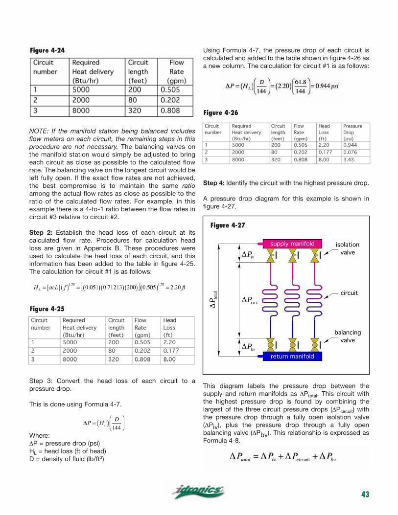
43

NOTE: If the manifold station being balanced includes flow meters on each circuit, the remaining steps in this procedure are not necessary. The balancing valves on the manifold station would simply be adjusted to bring each circuit as close as possible to the calculated flow rate. The balancing valve on the longest circuit would be left fully open. If the exact flow rates are not achieved, the best compromise is to maintain the same ratio among the actual flow rates as close as possible to the ratio of the calculated flow rates. For example, in this example there is a 4-to-1 ratio between the flow rates in circuit #3 relative to circuit #2.

Step 2: Establish the head loss of each circuit at its calculated flow rate. Procedures for calculation head loss are given in Appendix B. These procedures were used to calculate the heat loss of each circuit, and this information has been added to the table in figure 4-25. The calculation for circuit #1 is as follows:

Step 3: Convert the head loss of each circuit to a pressure drop.

This is done using Formula 4-7.

Where:∆P = pressure drop (psi)HL = head loss (ft of head)D = density of fluid (lb/ft3)

Using Formula 4-7, the pressure drop of each circuit is calculated and added to the table shown in figure 4-26 as a new column. The calculation for circuit #1 is as follows:

Step 4: Identify the circuit with the highest pressure drop.

A pressure drop diagram for this example is shown in figure 4-27.

This diagram labels the pressure drop between the supply and return manifolds as ∆Ptotal. This circuit with the highest pressure drop is found by combining the largest of the three circuit pressure drops (∆Pcircuit) with the pressure drop through a fully open isolation valve (∆Piv), plus the pressure drop through a fully open balancing valve (∆Pbv). This relationship is expressed as Formula 4-8.

Figure 4-24

Figure 4-25

∆Piv

∆Pcirc

∆Pbv

supply manifold

return manifold

isolation!valve

circuit

balancing!valve

∆P to

tal

Figure 4-27

Figure 4-26

44

The pressure drop of the isolation valve and balancing valve in the circuit with the largest circuit pressure drop are based on the Cv of these valves in their fully open positions. These pressure drops can be determined using Formula 4-9.

Where∆P = pressure drop through fully open valve (psi)D = density of fluid (lb/ft3)Cv = Cv flow coefficient for valve (from manufacturer’s specifications)f = flow rate through valve (gpm)

Since circuit #3 has the highest circuit pressure drop, the pressure drops through the isolation valve and balancing valve are determined at the flow rate through circuit #3.

Assume all isolation valves in the manifold station have a Cv of 3.2.

The pressure drop through the open isolation valve in circuit #3 at a flow rate of 0.808 gpm is:

Assume all balancing valves in the manifold station have a Cv of 2.1

The pressure drop through the fully open balancing valve in circuit #3 at a flow rate of 0.808 gpm is:

Hence the total pressure drop through circuit #3 is:

Step 5: Determine the differential pressure that must be absorbed by the balancing valves in the other circuits to equal the total pressure drop calculated in step 4.

This differential pressure can be determined using Formula 4-10.

circuit #1circuit #2

2.63 psi

0.50

5 gp

m

estimated setting = 1.6 turns open

3.50 psi

0.20

2 gp

m

estimated setting = 0.5 turns openFigure 4-28

Formula 4-9

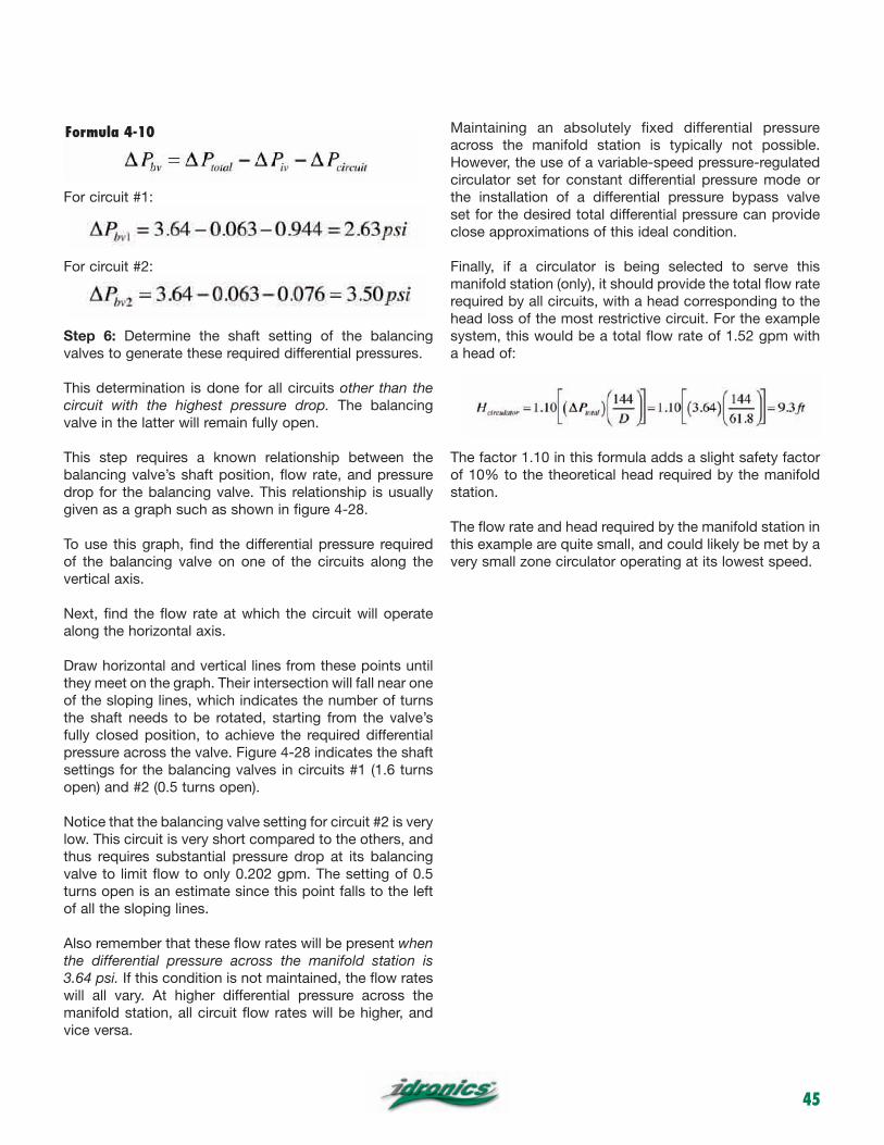
45

For circuit #1:

For circuit #2:

Step 6: Determine the shaft setting of the balancing valves to generate these required differential pressures.

This determination is done for all circuits other than the circuit with the highest pressure drop. The balancing valve in the latter will remain fully open.

This step requires a known relationship between the balancing valve’s shaft position, flow rate, and pressure drop for the balancing valve. This relationship is usually given as a graph such as shown in figure 4-28.

To use this graph, find the differential pressure required of the balancing valve on one of the circuits along the vertical axis.

Next, find the flow rate at which the circuit will operate along the horizontal axis.

Draw horizontal and vertical lines from these points until they meet on the graph. Their intersection will fall near one of the sloping lines, which indicates the number of turns the shaft needs to be rotated, starting from the valve’s fully closed position, to achieve the required differential pressure across the valve. Figure 4-28 indicates the shaft settings for the balancing valves in circuits #1 (1.6 turns open) and #2 (0.5 turns open).

Notice that the balancing valve setting for circuit #2 is very low. This circuit is very short compared to the others, and thus requires substantial pressure drop at its balancing valve to limit flow to only 0.202 gpm. The setting of 0.5 turns open is an estimate since this point falls to the left of all the sloping lines.

Also remember that these flow rates will be present when the differential pressure across the manifold station is 3.64 psi. If this condition is not maintained, the flow rates will all vary. At higher differential pressure across the manifold station, all circuit flow rates will be higher, and vice versa.

Maintaining an absolutely fixed differential pressure across the manifold station is typically not possible. However, the use of a variable-speed pressure-regulated circulator set for constant differential pressure mode or the installation of a differential pressure bypass valve set for the desired total differential pressure can provide close approximations of this ideal condition.

Finally, if a circulator is being selected to serve this manifold station (only), it should provide the total flow rate required by all circuits, with a head corresponding to the head loss of the most restrictive circuit. For the example system, this would be a total flow rate of 1.52 gpm with a head of:

The factor 1.10 in this formula adds a slight safety factor of 10% to the theoretical head required by the manifold station.

The flow rate and head required by the manifold station in this example are quite small, and could likely be met by a very small zone circulator operating at its lowest speed.

Formula 4-10

46

5. SYSTEMS USING PRESSURE-INDEPENDENT BALANCING VALVES

The pressure-independent balancing valves (PIBVs) discussed in section 3 make it easy to achieve and maintain fixed flow rates within each crossover and branch of a system.

When properly applied, PIBVs also minimize variations in flow rates as zone valves or thermostatic radiator valves begin closing within the system.

APPLICATION OF PIBVsPIBVs are rated for a specific flow rate. They will maintain this rated flow rate within a relatively narrow (+/- 5 %) tolerance provided that the differential pressure across them remains between a specific minimum and maximum value. This characteristic is shown in figure 5-1, where the minimum differential pressure is 2 psi, and the maximum differential pressure is 32 psi. These minimum and

maximum differential pressure thresholds vary with the type and size of the PIBV.

Consider the situation shown in figure 5-2. It consists of eight crossovers, each with a terminal unit, zone valve, and a PIBV. The PIBVs have been selected for the different design flow rates required for each crossover.

The operation of this system with all zones on, along with the associated head distribution, is shown in figure 5-3.

For proper operation, the PIBV in the flow path having the greatest hydraulic resistance must have a differential pressure across it that is at least as high as its minimum activation threshold (typically 2, 4, or 5 psi, depending on the PIBV used).

If the terminal units are similar or identical, and thus all operate at approximately the same flow rate, it is likely that the flow path through the crossover furthest from the circulator will have the highest hydraulic resistance.

If the terminals units are significantly different, and operate at significantly different flow rates, the flow path of greatest hydraulic resistance must be determined by calculating the head loss along the flow path through each crossover at its design flow rate, and comparing the results for the highest total head loss.

The circulator should be sized to provide the design flow rate when all zones are open, with a head output equal to the head loss of the most restrictive flow path. The latter must include the head loss of the supply/return mains, crossover piping, terminal unit, and the minimum operating differential pressure of the PIBV.

The calculation for head loss will typically require the head loss of each segment of the supply and return mains, out to and back from the most restrictive crossover, to be individually calculated and then added together. A method for making these head loss calculations is given in Appendix B.

flow rate

diffe

rent

ial p

ress

ure

2 psi

32 psipressure drop curve of PIBV when spring!is fully compressed

pressure drop curve of PIBV when spring!is fully extended

desirable working!range of

PIBV

rated flow rate of PIBV

terminal!unit #4

terminal!unit #3

terminal!unit #2

terminal!unit #1

terminal!unit #8

terminal!unit #7

terminal!unit #6

terminal!unit #5

heat input

PIBVs

10 g

pm

4 gp

m

6 gp

m

2 gp

m

8 gp

m

4 gp

m

3 gp

m

5 gp

m

Figure 5-1

Figure 5-2

47

This head loss could also be estimated by assuming a typical mains piping sizing criteria of 3 to 5 feet of head loss per hundred feet of pipe.

Example: Assume the mains piping in the system shown in figure 5-4 has been sized for a head loss of 5 feet per 100 feet of pipe. All terminal units are identical, and require 4 gpm when operating. All have the same 6 feet of head loss at their operating flow rate. The minimum operating pressure differential of

the PIBV is 2 psi. The system operates with water at an average temperature of 140 ºF. Determine the minimum circulator flow/head requirement for this system.

Solution: The total head loss of the flow path through the most remote heat emitter is the head loss of the mains, plus the head loss of the heat emitter, plus the minimum operating head loss of the PIBV. These can be determined separately and then added.

head loss across each terminal

unit & zone valve

head absorbed by each PIBV he

ad in

put

of c

ircul

ator

head loss along supply main

head loss along return main

flow rate (gpm)

0

2

4

6

8

10

12

14

16

18

0 2 4 6 8 10 12 14 16 18 20 22 24 26 28 30

head

lost

/ ad

ded

(feet

)

system head loss curve !(all 8 zones on)pump curve

minimum head loss for PIBV to maintain constant flow

Equal head loss and differential pressure !maintained across all crossovers

terminal!unit #4

terminal!unit #3

terminal!unit #2

terminal!unit #1

terminal!unit #8

terminal!unit #7

terminal!unit #6

terminal!unit #5

heat input

PIBVs

10 g

pm

4 gp

m

6 gp

m

2 gp

m

8 gp

m

4 gp

m

3 gp

m

5 gp

m

fixed speed

circulator

flow rate

diffe

rent

ial p

ress

ure

∆P min

pressure drop curve of PIBV when spring!is fully compressed

pressure drop curve of PIBV when spring!is fully extended

desireable working!range of

PIBV

rated flow rate of PIBV!in branch with highest!hydraulic resistance

∆P max

Figure 5-3

48

The head loss of each heat emitter is 6 feet at the desired operating flow rate of 4 gpm.

The minimum required head loss of the PIBV needs to be calculated from its minimum required pressure drop. This requires the density of water at an average temperature of 140 ºF, which is 61.3 lb/ft3. The head loss across the PIBV, which has an assumed minimum operating pressure of 2 psi, is then calculated as follows:

The total head loss through the most restrictive flow path can now be found by adding these individual head losses together:

The minimum operating requirement for the circulator is thus the total flow rate of all crossovers (e.g., 6 x 4 gpm = 24 gpm) at 23.7 feet of head, as shown in figure 5-5. The pump curve shown slightly exceeds the minimum operating point, and thus would be an acceptable choice.

When one or more of the zone valves in the system close, the operating point shifts left and upward along the pump curve. This increases the head available across the supply and return mains. The PIBVs in the active crossovers immediately react to absorb the extra head input, and thus maintain the same differential pressure across the active

crossovers. This reaction, depicted in figure 5-6, allows the flow rates in the active crossovers to remain unchanged.

There is no need to use a differential pressure bypass valve in a system equipped with PIBVs on each crossover. The PIBVs directly absorb the excess circulator head under partial load conditions.

USING PIBVs WITH VARIABLE-SPEED CIRCULATORS:It is possible to use variable-speed pressure-regulated circulators with PIBVs. Such circulators can reduce speed in response to attempted pressure increases caused by closing zone valves. This allows for significant reduction in circulator input power, and thus reduces electrical energy consumption. The excess head energy that would have been produced by a fixed-speed circulator, and ultimately dissipated through the PIBVs, is simply not

heat!emitter

heat input

PIBVs4

gpm

4 gp

m

4 gp

m

4 gp

m

4 gp

m

4 gp

m

130 ft

mains sized for head loss of 5 ft/100 ft

circ

ulat

or

heat!emitter

heat!emitter

heat!emitter

heat!emitter

heat!emitter

flow rate (gpm)

0

2

4

6

8

10

12

14

16

18

0 2 4 6 8 10

head

lost

(fee

t)

head loss curve!for each !

heat emitter

flow rate (gpm)

0

4

8

12

16

0 2 4 6 8 10 12 14 16 18 20 22 24 26 28 30

head

lost

/add

ed (f

eet)

minimum required operating point

pump curve that slightly exceeds operating point

20

24

28

32(24 gpm@23.7 ft head)

actual operating point using circulator!with pump curve shown

Figure 5-4

Figure 5-5

49

added to the system when a variable-speed pressure-regulated circulator is used.

A variable-speed, pressure-regulated circulator, operating in proportional differential pressure mode, and supplying a system using zone valves and manually set balancing valves, does reduce flow rate variations in active crossovers, when other crossovers are off. However, some variations in active crossover flow rates will still occur. Crossovers nearer the circulator tend to experience a nominal drop in flow rate, while those further from the circulator will experience a nominal gain in flow rate.

Assuming the hydraulic resistance of the crossovers is similar or identical, the extent of the flow rate variations depends on the piping used for the mains.

To maintain minimal variation on crossover flow rates, PIBVs can be used in combination with a variable-speed, pressure-regulated circulator operating in proportional differential pressure mode.

As is true with a fixed-speed circulator, the PIBVs require a minimum threshold differential pressure to maintain constant flow rates. The control curve on which the

terminal!unit #3

terminal!unit #3

terminal!unit #3

terminal!unit #4

terminal!unit #3

terminal!unit #1

terminal!unit #8

terminal!unit #6

heat input

head loss along supply main

head loss across each terminal

unit & zone valve

head absorbed by each PI balancing valve!

(all zones on)

head

inpu

t of

circ

ulat

or

head loss along return main

additional head absorbed by PI balancing valves

with some zones off

flow rate (gpm)

0

2

4

6

8

10

12

14

16

18

0 2 4 6 8 10 12 14 16 18 20 22 24 26 28 30

head

lost

(fee

t)

system head loss curve !(all 8 zones on)

pump curve system head loss curve!

(4 zones on)

addi

tiona

l hea

d ab

sorb

ed b

y PI

ba

lanc

ing

valv

es w

ith s

ome

zone

s of

fm

inim

um h

ead

loss

for

PI b

alan

cing

val

ve t

o m

aint

ain

cons

tant

flow

OFF OFF OFF

4 gp

m

2 gp

m

8 gp

m

3 gp

m

5 gp

m

Equal head loss and differential pressure !maintained across all crossovers

Figure 5-6

50

variable-speed circulator operates must not allow the differential pressure across the crossover with the highest hydraulic resistance to fall below the total of this minimum differential pressure plus the pressure drop of the other crossover piping components and piping mains when operating. The concept is shown in figure 5-7.

At design load conditions, all zone valves are open, and a properly sized variable-speed, pressure-regulated circulator will operate at or close to full speed. The pump curve and system head loss curve intersect at the upper operating point. The value of the circulator’s head at this design load condition is designated as “H.”

The standard control curve for a variable-speed, pressure-regulated circulator operating in proportional differential pressure mode is a line that passes through the design head requirement at full speed, and through 50 % of this design head requirement, (H/2), at zero flow rate. This standard

control curve is shown as a black line in figure 5-7.

When the circulator detects the closure of one or more zone valves, it reduces speed in an attempt to move the operating point down the control curve. For comparison, the operating point corresponding to 50 % system flow is shown in figure 5-7.

The solid green dot on the vertical axis represents the activation head for the PIBV, plus the design head loss of the piping components and terminal unit in the most remote crossover. The upward curvature is caused by increasing head loss of the mains piping as more zones become active.

To ensure that the activation condition of the PIBV in the most remote crossover is met, the left end of the variable-speed circulator’s control curve must be equal to, or (preferably) slightly higher than the green dot. This is the case in figure 5-7. Furthermore, the control curve must remain above the green dashed curve at all flow rates.

flow rate (gpm)

4

8

12

16

0 2 4 6 8 10 12 14 16 18 20 22 24 26 28 30

head

lost

/add

ed (f

eet) system head loss curve!

(all zone valves open)

pump curve @ 100% speed

20

24

28

32

control curve of variable speed circulator!when operating in proportional ∆P mode

pump curve @ 50% system flow

system head loss curve!(50% of zone valves open)

HH/

2

0

minimum head loss required to activate PIBV + head loss of mains piping to and from crossover having highest hydraulic resistance

operating point!(all zone valves open)

operating point!(50% of zone valves open)

0

10

2030

4050

60

7080

90100

0 10 20 30 40 50 60 70 80 90 100

% d

esig

n lo

ad c

ircul

ator

pow

er

% design load flow rate

fixed speed circulator

variable-speed, pressure-regulated! circulator in proportional ∆P mode!

in system with PIBVs

Figure 5-7

Figure 5-8

51

ENERGY SAVINGS USING VARIABLE-SPEED CIRCULATOR AND PIBVs:Analysis of systems that combine PIBVs and variable-speed, pressure-regulated circulators operating with proportional differential pressure mode show significant reductions in circulator input power at partial load conditions.

Figure 5-8 shows the estimated reduction in circulator input wattage for an eight-zone direct return system using PIBVs and either a fixed-speed or variable-speed, pressure-regulated circulator.

The system using a variable-speed, pressure-regulated circulator shows input wattage dropping to approximately 30 % of it nominal value at full load wattage when the system is operating at 50 % flow. The same system using a fixed-speed circulator draws about 70 % of its full-speed wattage when operating at 50 % flow in a system with PIBVs. The overall pumping energy savings of the variable-speed circulator over the life of the system will be substantial.

6. BALANCING INJECTION MIXING SYSTEMS

Injection mixing is one method of supplying heat produced by a conventional (e.g., higher temperature)

boiler to a low temperature distribution system. It is accomplished by pushing hot water into a tee within the circulating lower temperature distribution system, while simultaneously removing cooler water through another tee, as shown in figure 6-1.

There are several hardware options that can be used for injection mixing. The two methods discussed in this issue of idronics include:

• Injection mixing using a two-way modulating valve• Injection mixing using a variable-speed pump

Both of these approaches require proper valve selection and balancing for optimum performance.

INJECTION MIXING WITH 2-WAY MODULATING VALVESA 2-way modulating valve assembly consists of a valve body and an actuator that moves the stem of the valve. This assembly regulates the rate of hot water flow from a boiler loop into the lower temperature distribution system, as shown in figure 6-2.

A metered balancing valve is installed in the return injection riser. Its purpose is to indicate the injection flow rate and, when necessary, allow the flow resistance of the injection riser to be increased to properly tune the system.

distribution system

heated water injection riser

cool water outlet riser

mixing BEGINS within this tee

supply temperature sensor!(preferred location)

purging valve

do NOT place supply temperature sensor here!

Figure 6-1

52

For optimal performance, the injection control valve and the flow-restrictor valve need to be properly selected and adjusted. The following selection and adjustment procedure applies to both 2-way thermostatic and 2-way motorized injection control valves.

Step 1: Determine the required injection flow rate under design load conditions. This can be determined using Formula 6-1.

Where:fi = required injection flow rate at design load (gpm) Q = rate of heat transfer to distribution system at design load (Btu/hr)∆T = temperature difference between supply and return injection risers (ºF)k = a constant depending on fluid used (for water k=490, for 30% glycol solution k=479, for 50% glycol solution k=450)

Step 2: Determine the flow rate through the distribution system under design load conditions using Formula 6-2.

Where:fsystem = flow rate in distribution system at design load (gpm) Q = rate of heat transfer to distribution system at design load (Btu/hr)∆T = temperature drop of distribution system at design load (ºF)k = a constant depending on fluid used (for water k=495, for 30% glycol solution k=479, for 50% glycol solution k=450)

Step 3: Select a valve body for the injection control valve. The Cv of this valve body should be approximately equal to the calculated injection flow rate from step 1.

Step 4: Calculate the Cv of the flow-restrictor valve using Formula 6-3:

VENT

conventional boiler

distribution system

2-way motorized injection valve and actuator

flow!restrictor!valve

metered balancing valve

supply temperature sensoroutdoor temperature sensor

closely spaced tees

boiler inlet temperature sensor

mixing controller

Figure 6-2

Formula 6-1

Formula 6-2

53

Where:Cvfrv = Cv required of flow-restrictor valvefsystem = flow rate in distribution system at design load (gpm)Cvi = Cv of selected injection control valvefi = required injection flow rate at design load (gpm)

Select a globe-type flow-restrictor valve with a Cv approximately equal to that calculated using Formula 6-3.

The metered balancing valve should be selected with a scale that goes at least as high as the design injection flow rate calculated using Formula 6-1.

After the hardware is sized and installed, it needs to be “tuned” for optimal performance. As a result of tuning, the injection control valve should be fully open at design load conditions.

The following procedure is used to tune the injection mixing assembly:

Step 1: After the system is filled and purged of air, fully open the flow-restrictor valve, the injection control valve and the metered balancing valve. If the distribution system is zoned, open all zones so flow through the distribution system represents design load conditions. The actuator on the injection control valve may have to be temporarily removed to ensure the valve is fully open.

Step 2: Turn on the boiler circulator and the distribution circulator, then read the flow rate – if any – passing through the metered balancing valve in the injection riser.

Step 3: If the flow rate indicated by the metered balancing valve is higher than the calculated injection flow rate, slowly close the plug on the metered balancing valve until the flow reading equals the calculated injection flow

VENT

conventional boiler

distribution system

closely spaced tees

boiler inlet temperature!

sensor

closely spaced teesinjection risers

injection controller18

" m

inim

um

metered!balancing!

valve

variable speed !injection pump

boiler loop

outdoor!temperature!

sensor

purging!valve

Figure 6-3

Formula 6-3

54

rate. Procede to step 5.Step 4: If the flow reading on the metered balancing valve is lower than the calculated injection flow rate, slowly begin to close the flow-restrictor valve until the flow rate on the metered balancing valve equals the calculated injection flow rate. Leave the metered balancing valve set in the fully open position.

Step 5: Mark and/or note the position of each valve stem. Reinstall the actuator on the injection control valve. The tuning procedure is complete.

INJECTION MIXING WITH A VARIABLE-SPEED CIRCULATORAnother popular method of accomplishing injection mixing uses a variable-speed pump as the injection control device. The most common piping for this approach is shown in figure 6-3.

The power requirement for an injection pump operating in a residential-size system, with relatively short (2- to 4-foot long) injection risers is extremely low. For example, a system with 8 feet of 1/2-inch copper injection riser piping operating at an injection flow rate of 2 gpm requires less than 1 watt of electrical input power to the injection pump (assuming a 25% wire-to-water efficiency). Such ultra-low wattage circulators are currently not available in the North American market. Thus it is common to use a small “zone circulator” as the injection pump.

Although a typical zone circulator is acceptable, it is far more powerful, even at only 40 watts power input, than what is needed for proper injection flow in most residential and light commercial systems.

If a zone circulator is installed as the injection pump, it will seldom operate at more than 10% of full speed. This effectively wastes 90% of the speed adjustment range of that circulator, and reduces the ability of the mixing assembly to fine-tune supply water temperature.

One solution is to install a metered balancing valve in one of the injection risers to significantly increase the head against which the injection pump operates. The flow resistance created by this valve significantly steepens the head loss curve of the injection risers, as shown in figure 6-4.

The goal in setting the metered balancing valve is to allow the calculated design load injection flow rate through the injection risers, while the injection pump operates at full speed.

For example: Assume the design injection flow rate is

2 gpm. By progressively closing the metered balancing valve, the head loss curve in figure 6-3 steepens from its original position (shown in blue dashed lines) to a position where it intersects the pump curve at the desired flow rate of 2 gpm. The pump curve is for a small (1/40 horsepower) circulator operating at full speed. Once this intersection is achieved, the metered balancing valve is properly set.

The following procedure can be used to properly set the metered balancing valve.

Step 1: Calculate the necessary injection flow rate under design load conditions. The procedure is identical to that described for injection mixing with valves. Use Formula 6-1:

Where:fi = required injection flow rate at design load (gpm) Q = rate of heat transfer to distribution system at design load (Btu/hr)∆T = temperature difference between supply and return injection risers (ºF)

0

1

2

3

4

5

6

7

8

9

0 1 2 3 4 5 6 7 8 9 10

head

(fee

t)

flow rate (gpm)

pump curve for 1/40 HP!circulator at 100% speed

operating point at design injection !flow rate with circulator at 100% speed

head loss of injection riser piping with!properly adjust flow restrictor valve

head loss of injection riser piping!without flow restrictor valve

closing flowrestrictor valve

Figure 6-4

Formula 6-1

55

Step 2: Once the injection flow rate is calculated, turn on the injection pump at full speed. For AC circulators, this can be done by either setting the injection controller to full-speed mode or by wiring a line cord to the circulator and plugging it in. If a multi-speed injection pump is used, set it for the lowest speed setting.

Step 3: Begin reducing flow through the metered balancing valve until the indicated flow rate matches the calculated design injection flow rate. If this cannot be achieved with the pump on its low speed setting, change to higher speeds – as required – to achieve the required injection flow rate. The flow restrictor valve is now properly set.

SUMMARYProper balancing of hydronic systems is an essential step in achieving optimal performance. The methods presented in this issue of idronics represent straightforward procedures for determining the flow rates in each portion of a system, and then setting the balancing valves to achieve these flow rates.

Again, the ultimate goal of balancing is to ensure proper rate of heat delivery to each space served by the system. In theory, this can be achieved by adjusting balancing valves to calculated settings. These settings are based on predetermined flow rates, which are based on calculated loads. If the actual loads of the building are exactly the same as the calculated loads, these procedures should yield a perfectly balanced system. However, some variation between calculated loads and actual loads is common. In such cases, the balancing procedures described should allow the system to approach an ideal balanced condition. However, some “fine-tuning” of the balancing valves beyond their calculated setting may still be necessary to achieve optimal comfort conditions.

Of all the system configurations discussed, those that combine pressure-independent balancing valves (PIBVs) with a variable-speed, pressure-regulated circulator have the best potential of producing predictable and stable flows, while significant reducing circulator energy usage.

56

circulator

circulator w/!isolation flanges !

circulator w/!internal check valve!& isolation flanges !

gate valve

globe valves

ball valve

thermostatic!radiator valve

thermostatic!radiator valve

strainer

primary/secondary!fitting

cap

hose bib!drain valve

diverter tee

union

pressure gauge

diaphragm-type !expansion tank

3-way motorized mixing valve

4-way motorized mixing valve

swing check valve

spring loaded!check valve

purging valve

metered balancing valve

pressure relief valve

brazed !plate!heat !exchanger

Modulating / condensing boiler

conventional boiler

GENERIC COMPONENTS

indirect water heater (with trim)

pressure & temperature relief valve

CALEFFI COMPONENTS

Modulating tankless water heater

solar collector array

DISCAL central!air separators !

backflow preventer

pressure reducing!valve

zone valve!(2 way)

zone valve!(3 way)

float -type!air vent

3-way !thermostatic mixing valve

flow-check !valve

differential !pressure!bypass valve

VENT

Hydro Separator

Hydrolink!(3 configurations)

manifold station with balancing valves

pressure!relief valve

air & dirt!separatorDIRTCAL!

dirt separator

high temperature!solar DISCAL !air separators !

high temperature!solar pressure!relief valve!

high temperature!solar air vent

high temperature!solar 3-way thermostatic!mixing valve

high temperature!solar !expansion!tank

isolar !differential temperature controller

flowcal!balancing!valves

high temperature!shut-off valve for!solar air vent

solar!circulation!station

mixing units!(2 configurations)

distribution!station

balancing!valve w/!flowmeter

3-way thermostatic!mixing valve

APPENDIX A: PIPING SYMBOL LEGEND

57

APPENDIX B: HEAD LOSS CALCULATION METHOD

The balancing concepts and procedures discussed in this issue often make reference to the head loss of a piping circuit or piping path. This appendix presents a simple method for calculating the head loss of piping paths or circuits constructed of smooth tubing (copper, PEX, PEX-AL-PEX, PP).

The head loss of a piping path or circuit can be determined using Formula B-1.

HL = Head loss of circuit (ft of head)a = a factor that depends on the fluid used in the system, and that fluid’s average temperature (see figure B-1)c = a factor determined by the type and size of tubing in the circuit (see figure B-2)l = total equivalent length of the circuit (ft) (see figure B-3)f = flow rate (gpm)1.75 = an exponent of flow rate

The values of “a” read from figure B-1 should be based on the average fluid temperature within the system at design load conditions. Thus, for a system with a design supply temperature of 150ºF and a return temperature of 130ºF, the value of “a” would be determined at the average fluid temperature of 140ºF.

The equivalent length “L” for a segment of pipe is simply its length. The equivalent resistance of a fitting or valve can be found in the table shown in figure B-3.

For example, the equivalent length of a 1”-size 90º copper elbow would be 2.5 feet of 1” copper tube. If a circuit path contained 3 such elbows, their total equivalent length would simply be 3 x 2.5 ft = 7.5 feet. The equivalent lengths of fittings and valves would be added to the linear length of tubing in the circuit path to get a total equivalent length for that path.

Example: A circuit contains 150 feet of ¾” copper tubing, eight 90º elbows, and 2 ball valves. It is supplied with water at 120 ºF and operates with a design load temperature drop of 20 ºF and flow rate of 3.5 gpm. Determine the head loss of this circuit.

0.04

0.05

0.06

0.07

0.08

0.09

0.1

50 70 90 110 130 150 170 190 210

"a"

valu

e fo

r flui

d

average fluid temperature (ºF)

50% propylene glycol

30% propylene glycol

water

Tube (size & type) C value3/8" type M copper 1.01641/2" type M copper 0.333523/4" type M copper 0.0619571" type M copper 0.01776

1.25" type M copper 0.00680821.5" type M copper 0.00306672" type M copper 0.0008331

2.5" type M copper 0.00029773" type M copper 0.0001278

3/8" PEX 2.93361/2" PEX 0.7865/8" PEX 0.29473/4" PEX 0.142031" PEX 0.04318

1.25" PEX 0.016681.5" PEX 0.0075542" PEX 0.002104

3/8" PEX-AL-PEX 3.354181/2" PEX-AL-PEX 0.61625/8" PEX-AL-PEX 0.195063/4" PEX-AL-PEX 0.063791" PEX-AL-PEX 0.019718

Formula B-1

Figure B-1

Figure B-2

58

Solution: The total equivalent length of the circuit is 150 feet, plus 2 feet for each elbow, and 2.2 feet for each ball valve. This totals to 170.4 feet. The equivalent lengths of the elbows and valves were read from figure B-3.

The average water temperature in the system is the supply temperature minus one half the temperature drop, or 120-(20/2)=110ºF.

The “a” value of water at an average temperature of 110ºF is 0.051.

The “c” value for ¾” copper tubing is 0.061957.

Putting these values into Formula B-1 yields:

Figure B-3

59

APPENDIX C: THERMAL MODEL FOR A RADIANT PANEL CIRCUIT

Formula C-1 can be used to determine the outlet temperature of a specific radiant panel based on its construction and the conditions under which it operates:

Where:

Tout = fluid outlet temperature for baseboard (ºF)Tin = fluid inlet temperature to baseboard (ºF)Troom = temperature of room air entering baseboard (ºF)a = thermal output parameter for a specific panel constructionl = length of radiant panel circuit (ft)c = specific heat of fluid flowing through circuit based on its average temperature (Btu/lb/ºF)D = density of fluid in circuit based on it average temperature (lb/ft3)f = flow rate through circuit (gpm)e = 2.71828 (base of natural logarithm system)

Once the outlet temperature for the panel is determined, it can be combined with the inlet temperature and flow rate to determine the total heat output. Use Formula C-2 for this calculation.

Where:

Toutlet = outlet temperature of fluid leaving radiant panel (ºF)Tinlet = fluid temperature at inlet of radiant panel (ºF)D = density of fluid within baseboard (lb/ft3)c = specific heat of fluid within baseboard (Btu/lb/ºF)ƒ = fluid flow rate through the baseboard (gpm)

The value of “a” in Formula 2-3 is based on the exact construction of the radiant panel, including tube spacing, tubing embedment method, finish floor coverings, and underside insulation. This value can be determined based on a known relationship between heat output, and a corresponding circuit water temperature and room air temperature. The relationship is given as Formula C-3.

Where:s =tubing spacing (inches)Qup = upward heat flux from panel (Btu/hr/ft2)Qdown = downward heat flux from panel (Btu/hr/ft2)Tw = water temperature in circuit corresponding to the above heat outputs (ºF)Troom = room air temperature corresponding to the above heat outputs (ºF)

Example: A radiant floor panel with 12” tube spacing creates an average upward heat output of 25 Btu/hr/ft2, with a corresponding downward heat loss of 2 Btu/hr/ft2. The average water temperature in the radiant panel circuit at these conditions is 110ºF, and the room air temperature above the panel is 70ºF. Determine the value of “a” for use in Formula C-3.

Solution:

Example: Assume a radiant floor panel consists of a single 300-foot-long circuit of ½” PEX tubing, spaced 12-inches apart. When operating at an average water temperature of 110ºF this panel’s average upward heat output is 25 Btu/hr into a room at 70ºF, and its downward heat output is 2.5 Btu/hr. Further assume that the radiant panel circuit is supplied with water at a temperature of 120ºF and flow rate of 0.8 gpm. Determine:

a. The “a” value of the panelb. The total heat transfer from the radiant panelc. The total upward heat transfer from the radiant panel

Solution: The value of “a” can be determined from the given data using Formula C-3:

It is necessary to determine the density and specific heat of the water at its average temperature before using Formula 2-3. However, the average water temperature of the circuit is not known at this point. As an approximation, assume a temperature drop along the circuit of 20ºF. Under this assumption, the average water temperature would be 120-(20/2) = 110ºF. The density of water at 110ºF is 61.8 lb/ft3. The specific heat of water at this temperature is 1.00 Btu/lb/ºF. This data, along with the other stated and calculated numbers, are now used in Formula C-1 to determine the circuit’s outlet temperature.

Formula C-1

Formula C-2

Formula C-3

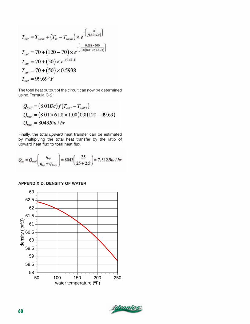
60

The total heat output of the circuit can now be determined using Formula C-2:

Finally, the total upward heat transfer can be estimated by multiplying the total heat transfer by the ratio of upward heat flux to total heat flux.

APPENDIX D: DENSITY OF WATER

58

58.5

5959.5

6060.5

61

61.562

62.563

50 100 150 200 250

dens

ity (l

b/ft3

)

water temperature (ºF)

Function

Technical specifications

Product range

120 series FlowCal Y-strainer with integral ball valve, with and without pressure and temperature test ports ..................................................................................................................................................... sizes 1/2”, 3/4”, 1”, 1-1.4” NPT or Sweat

125 series FlowCal Y-strainer in standard configuration, with and without pressure and temperature test ports ............................................................................................................................................................... sizes 1/2”, 3/4”, 1", 1-1/4” NPT only

series 120 - 125 series

FlowCal™ Y-Strainer

CALEFFI

The FlowCal Y-strainers include a combination Y-strainer with integral ball valve (120 series) or a standard configuration Y-strainer without ball valve (125 series). Inspection, cleaning, and replacing the strainer cartridge can be done easily without removing the body from the pipleine. All configurations are available with optional factory-installed pressure and temperature test ports. Drain valves are also available as an accessory for installing in the blowdown port connection.

MaterialsBody: brassStrainer cartridge: stainless steelSeals: EPDMBall: brass, chrome-platedBall and control stem seal: PTFELever: special zinc-plated steelIdentification: metal plate with ball chain stating mesh size

PerformanceMedium: water, glycol solutionsMax. percentage of glycol: 50%Max. working pressure: 400 psi (400 WOG) Working temperature range: 32-212°F (0-100°C)Strainer mesh diameter: 0.87 mm (20 mesh)Connections: 1/2”, 3/4”, 1“, 1-1/4” NPT or Sweat (120 only)Cv: 1/2”: 8.0; 3/4”: 8.4; 1”:19.3; 1-1/4”: 20.0

Dimensions

A1/2"3/4"1"

1 1/4"

B6 3/16”6 1/4”8 5/8”

8 11/16”

C1 15/16”1 15/16”3 3/4”3 3/4”

D1 15/16”1 15/16”2 5/8”2 5/8”

E3 15/16”3 15/16”4 3/4”4 3/4”

F1/4"1/4"1/2"1/2"

A1/2"3/4"

1"1 1/4"

B4”

4 3/16”

5 13/16”

C1 15/16”1 15/16”3 3/4”3 3/4”

F1/4"1/4"1/2"1/2"

Code12014 ...12015 ...12016 ...12017 ...

Code12514 ...12515 ...12516 ...12517 ...

Weight (lb)

3.003.006.006.00

Weight (lb)

1.401.402.603.00

5 13/16”

E

A

C

F

B

D

A CALEFFI

AC

F

B

D

A CALEFFI

61

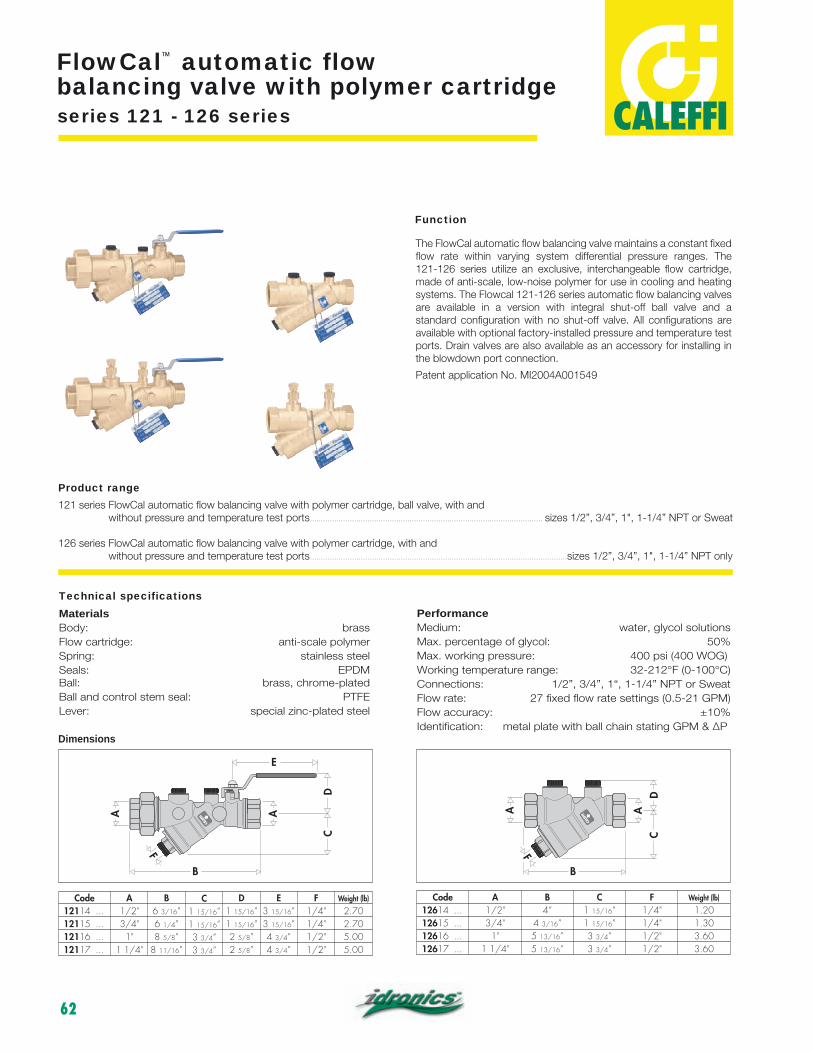
Function

Technical specifications

Product range121 series FlowCal automatic flow balancing valve with polymer cartridge, ball valve, with and without pressure and temperature test ports......................................................................................................... sizes 1/2”, 3/4”, 1", 1-1/4” NPT or Sweat

126 series FlowCal automatic flow balancing valve with polymer cartridge, with and without pressure and temperature test ports.................................................................................................................... sizes 1/2”, 3/4”, 1", 1-1/4” NPT only

series 121 - 126 series

FlowCal™ automatic flowbalancing valve with polymer cartridge

CALEFFI

The FlowCal automatic flow balancing valve maintains a constant fixed flow rate within varying system differential pressure ranges. The 121-126 series utilize an exclusive, interchangeable flow cartridge, made of anti-scale, low-noise polymer for use in cooling and heating systems. The Flowcal 121-126 series automatic flow balancing valves are available in a version with integral shut-off ball valve and a standard configuration with no shut-off valve. All configurations are available with optional factory-installed pressure and temperature test ports. Drain valves are also available as an accessory for installing in the blowdown port connection.

Patent application No. MI2004A001549

MaterialsBody: brassFlow cartridge: anti-scale polymerSpring: stainless steelSeals: EPDMBall: brass, chrome-platedBall and control stem seal: PTFELever: special zinc-plated steel

PerformanceMedium: water, glycol solutionsMax. percentage of glycol: 50%Max. working pressure: 400 psi (400 WOG) Working temperature range: 32-212°F (0-100°C)Connections: 1/2”, 3/4”, 1“, 1-1/4” NPT or SweatFlow rate: 27 fixed flow rate settings (0.5-21 GPM)Flow accuracy: ±10%Identification: metal plate with ball chain stating GPM & ∆P

Dimensions

E

A1/2"3/4"1"

1 1/4"

B6 3/16”6 1/4”8 5/8”

8 11/16”

C1 15/16”1 15/16”3 3/4”3 3/4”

D1 15/16”1 15/16”2 5/8”2 5/8”

A

C

F

B

D

A

E3 15/16”3 15/16”4 3/4”4 3/4”

F1/4"1/4"1/2"1/2"

A1/2"3/4"

1"1 1/4"

B4”

4 3/16”

5 13/16”

C1 15/16”1 15/16”3 3/4”3 3/4”

AC

F

B

D

A

F1/4"1/4"1/2"1/2"

Code12114 ...12115 ...12116 ...12117 ...

Code12614 ...12615 ...12616 ...12617 ...

Weight (lb)

2.702.705.005.00

Weight (lb)

1.201.303.603.60

CALE

FFI

CALE

FFI

5 13/16”

62

Construction details

Operating principleThe FlowCal flow cartridge is composed of a cylinder, a spring-loaded piston, and a combination of fixed and variable geometric orifices through which the fluid flows. These variable orifice sizes increase or decrease by the piston movement, contingent on the system’s fluid thrust. A specially calibrated spring counteracts this movement to regulate the amount of fluid which may pass through the valve orifices, maintaining a balanced system.

Polymer flow cartridge

The flow rate cartridge is made of an anti-scale polymer, specially engineered for use in cooling, heating and domestic water systems to prevent mineral buildup and is excellent in a wide range of working temperatures. It features high resistance to the abrasion caused by continuous fluid flow, it is insensitive to the deposit of scale and is fully compatible with glycols and additives used in circuits. The flow cartridge is able to accurately control the flow rate in a wide range of operating pressures. A special internal chamber acts as a damper for the vibrations triggered by the fluid flow, allowing low noise operating conditions to the device. It can be used in systems both on zone branch circuits and directly at the terminals.

System operation

If the differential pressure is within the control range (2 -14, 2 - 32, 4 - 34, 5 - 35, 3 - 32, 4 - 35 psid), the spring-loaded piston is positioned to give the fluid a free flow area permitting regular flow at the nominal rate for which the FlowCal is set up.

DIFFERENTIALPRESSURE *

FLOW RATE

G0

Control range

Initi

al ∆

p

Fina

l ∆p

2 psi 32 psi

Ball Valve

The control stem of the ball valve has a blowout-proof stem and the reversible closing lever is covered with vinyl.

Replaceable cartridge

The internal flow cartridge can be removed easily from the valve body for inspection, cleaning or replacement by unscrewing the cap as shown. Tools are not needed as the cartridge is removed with an integral retaining wire and ring.

cod.Q =R

ange ∆p =

m3/hkPa

15018

CALEFFI

CALEFFI

∆p (kPa)

cod.Q =R

ange ∆p =

m3/hkPa

15018

CALEFFI

CALEFFI

Pressure and temperature testing

The FlowCal body can be fitted with connections for the pressure and temperature ports, which is useful when checking operation in the working range. In addition, drain valve 538202 FD -1/4” NPT; 538402 FD -1/2” NPT, can be connected for blowdown operations.

Sizing the circuit with FlowCal

Size the hydronic system with FlowCal automatic balancing valves asfollows:

1. ∆PMAXCIRCUIT

Determine the pressure head loss for the zone circuit with the greatest pressure drop ( flow resistance). This is true for any hydronic system with supply and return headers.As an example, this would be circuit #8 for the 2-pipe direct return system with circuits having identical resistance, illustrated to the right, as it is farthest from the pump. If, however, all circuits are not identical, choose the circuit with the greatest pressure drop.

2. ∆PMINFLOWCAL

Add the minimum differential operating pressure(2, 4, or 5 psid) required for the FlowCal model selected for the circuit with the greatest pressure drop.

3. PUMP HEAD = ∆PMAXCIRCUIT + ∆PMINFLOWCAL

7654321 8

765432 81

∆p absorbed by Flowcal™at 100% load

extra ∆p absorbed by Flowcal™at 50% load

minimum ∆p requested byFlowcal™

H pump

∆p branch circuitat nominal flow rate

Terminal

∆p circuit (flow + return)

FlowCal™

Regulating valve

Differential pressures (∆p)

63

Function

Technical specifications

Product range

127 series FlowCal compact automatic flow balancing valve, with polymer cartridge, NPT or Sweat union sizes 1/2”, 3/4”, 1"

series 127

FlowCal™ compact automatic flowbalancing valve

CALEFFI

Dimensions

The FlowCal automatic flow balancing valve maintains a fixed flow rate within varying system differential pressure ranges. The design incorporates an exclusive flow cartridge, made of anti-scale, low-noise polymer and a compact low-lead brass valve body for use in cooling, heating and domestic hot water systems.

• Compact valve body with reduced dimensions

• Union connections for easy install into in-line pipes

• Ideal for zone applications or directly at the system’s terminal emitters

• Patent application No. MI2004A001549

MaterialsBody: low-lead brass (<0.25% Lead content)Flow cartridge: anti-scale polymerSpring: Stainless steelSeals: EPDM

PerformanceMedium: water, glycol solutionsMax. percentage of glycol: 50%Max. working pressure: 232 psi (16 bar)Working temperature range: 32-212°F (0-100°C)Connections: 1/2”, 3/4” and 1” NPT or Sweat unionFlow rate: 16 fixed flow rate settings ranging from 0.5 - 10 GPMFlow accuracy: ±10%Lead plumbing law compliance: (0.25% Max. weighted average lead content)

Agency approval: Lead plumbing law certified by IAPMO R&T

Code No. A B C Weight (lb)127341AF ... 1/2” NPT male union 5 13/16" 1 9/16" 1.0127349AF ... 1/2” Sweat union 4 1/4" 1 9/16" 0.8127351AF ... 3/4” NPT male union 5" 1 9/16" 1.0127359AF ... 3/4” Sweat union 4 13/16" 1 9/16" 0.8127361AF ... 1” NPT male union 5 5/8" 1 9/16" 1.2127369AF ... 1” Sweat union 6" 1 9/16" 1.0

B

C A A

Lead plumbing law certified by IAPMO R&T

64

Construction details

Operating principleThe FlowCal flow cartridge is composed of a cylinder, a spring-loaded piston, and a combination of fixed and variable geometric orifices through which the fluid flows. These variable orifice sizes increase or decrease by the piston movement, contingent on the system’s fluid thrust. A specially calibrated spring counteracts this movement to regulate the amount of fluid which may pass through the valve orifices, maintaining a balanced system.

FlowCal valves are high performance automatic flow balancing valves which control selected flow rates within a very tight tolerance (approximately 10%) and offer a wide range of operation.

The flow rate cartridge is made of an anti-scale polymer, specially engineered for use in cooling, heating and domestic water systems to prevent mineral buildup and is excellent in a wide range of working temperatures. It features high resistance to the abrasion caused by continuous fluid flow, it is insensitive to the deposit of scale and is fully compatible with glycols and additives used in circuits.

System operationIf the differential pressure is within the control range (2 -14, 2 - 32, 4 - 34, 5 - 35 psid), the spring-loaded piston is positioned to give the fluid a free flow area permitting regular flow at the nominal rate for which the FlowCal is set up.

DIFFERENTIALPRESSURE *

FLOW RATE G0

Control range

Initi

al ∆

p

Fina

l ∆p

2 psi 32 psi

FLU

ID T

HR

UST

Code Size Flow rate (gpm)127341AF • • • 1/2” NPT 0.50 0.75 1.00 1.50 2.50 3.00 3.50 4.00 4.50 5.00 6.00 7.00 8.00 9.00 10.00127341AF • • • 1/2” Sweat 0.50 0.75 1.00 1.50 2.50 3.00 3.50 4.00 4.50 5.00 6.00 7.00 8.00 9.00 10.00127341AF • • • 3/4” NPT 0.50 0.75 1.00 1.50 2.50 3.00 3.50 4.00 4.50 5.00 6.00 7.00 8.00 9.00 10.00127341AF • • • 3/4” Sweat 0.50 0.75 1.00 1.50 2.50 3.00 3.50 4.00 4.50 5.00 6.00 7.00 8.00 9.00 10.00127341AF • • • 1” NPT 0.50 0.75 1.00 1.50 2.50 3.00 3.50 4.00 4.50 5.00 6.00 7.00 8.00 9.00 10.00127341AF • • • 1” Sweat 0.50 0.75 1.00 1.50 2.50 3.00 3.50 4.00 4.50 5.00 6.00 7.00 8.00 9.00 10.00

* ∆p range (psid)2 - 142 - 324 - 345 - 35

* Minimum differential pressure required: This is equal to the minimum working ∆p of the FlowCal cartridge: 2, 4 or 5 psi (13, 27 or 34 kPa).

Exclusive design

With its exclusive design, the flow cartridge is able to accurately control the flow rate in a wide range of operating pressures. A special internal chamber acts as a damper for the vibrations triggered by the fluid flow, allowing low noise operating conditions to the device. It can be used in systems both on zone branch circuits and directly at the terminals.

Flow rate table

Ordering information for FlowCal 127 seriesSelect the appropriate valve for your application from the table at right. Then select the desired flow rate from the table below. When ordering, combine the appropriate Code No. from the table at right with the last 3 digits from the table below. Example: 127341AFG50.

CARTRIDGE LOCKING NUT

FLOW CARTRIDGEVALVE BODY

GPM Last 3 Digits of Code No. (...)

Pressure Differential Control Range (psid) GPM Last 3 Digits of Code

No. (...)Pressure Differential Control Range (psid)

0.5 G502 - 14

4 4G02 - 320.75 G75 4.5 4G5

1 1G0

2 - 32

5 5G01.5 1G5 6 6G0

4 - 342 2G0 7 7G02.5 2G5 8 8G03 3G0 9 9G0

5 - 353.5 3G5 10 10G

Code No. Description Code No. Description127341AF ... 1/2” NPT male union 127359AF ... 3/4” Sweat union

127349AF ... 1/2” Sweat union 127361AF ... 1” NPT male union

127351AF ... 3/4” NPT male union 127369AF ... 1” Sweat union

65

Function

Technical specifications

Product range

132 series QuickSetter balancing valve with flow meter sizes 1/2”, 3/4”, 1”, 1 1/4” and 1 1/2”

series 132

QuickSetter TM Balancing valve with flow meter

CALEFFI

Dimensions

The QuickSetter balancing valve accurately sets the flow rate of heating and cooling transfer fluid supplied to fan coils and terminal units or where flow balancing is required in solar thermal systems. Proper balancing ensures that the system operates according to design specifications, providing satisfactory thermal comfort with low energy consumption. A flow meter housed in a bypass circuit on the valve body facilitates flow rate adjustment and can be shut off during normal operation. The flow meter provides fast and easy circuit balancing without added differential pressure gauges and reference charts. The balancing valve is furnished with a pre-formed insulation shell to optimize thermal performance for both hot and cold water systems.

• Patent application No. MI2007A000703

MaterialsValve: - body: brass - ball: brass - ball control stem: brass, chrome plated - ball seal seat: PTFE - control stem guide: PSU - seals: EPDMFlow meter: - body: brass - bypass valve stem: brass, chrome plated - springs: stainless steel - seals: EPDM - flow meter float and indicator cover: PSU

PerformanceSuitable fluids: water, glycol solutionsMax. percentage of glycol: 50%Max. working pressure: 150 psi (10 bar)Working temperature range: 14 - 230°F (-10–110°C)Flow rate range unit of measurement: gpmAccuracy: ±10%Control stem angle of rotation: 90°Control stem adjustment wrench: Size 1/2”, 3/4”, 1 and 1 1/4”: 9 mm Size 1 1/2”: 12 mmThreaded connections: 1/2”- 1 1/2” FNPT

InsulationMaterial: closed cell expanded PE-XThickness: 25/64” (10 mm)Density: Inner part: 1.9 lb/ft3 (30 kg/m3) Outer part: 3.1 lb/ft3 (50 kg/m3)

Thermal conductivity (DIN 52612): At 32°F (0°C): 0.263 BTU·in/hr·ft2·°F (0.038 W/(m·K)) At 104°F (40°C): 0.312 BTU·in/hr·ft2·°F (0.045 W/(m·K))Coefficient of resistance to water vapor (DIN 52615): >1300Working temperature range: 32 - 212°F (0 - 100°C)Reaction to fire (DIN 4102): class B2

A B

CA

D

CALEFFI

7

6

5

4

3

2

D5 3/4 ”5 3/4 ”6 1/4 ”6 1/2 ”6 3/4 ”

C1 13/16”1 13/16”1 7/8 ”

2”2 1/4 ”

B3 5/16”3 5/16

3 3/8 ”3 1/2 ”3 5/8 ”

Weight (lb)1.71.02.12.63.2

A1/2”3/4”

1”1 1/4”1 1/2”

Code132432A132552A132622A132772A132882A

230°F

3/4” NPT

GPM

150 psi

66

Operating principleThe QuickSetter balancing valve is a hydraulic device that controls the flow rate of the heating/cooling transfer fluid.

The control mechanism is a ball valve (1), operated by a control stem (2). The flow rate is manually and properly set by use of the convenient onboard flow meter (3) housed in a bypass circuit on the valve body. This circuit is automatically shut off during normal operation. The flow rate is indicated by a metal ball (4) sliding inside a transparent channel (5) with an integral graduated scale (6).

Flow rate table

7

6

5

4

3

2

3

5

6

4

230°F

3/4” NPT

Bypass valveThe bypass valve (1) opens and closes the circuit between the flow meter and the valve. The bypass valve is easily opened by pulling the operating ring (2), and is automatically closed by the internal return spring (3) when finished reading the flow rate. The spring and the EPDM seal (4) provide a reliable seal to isolate the flow meter during normal operation.

3

2

1

1

234

4

6

7

5

Code 132432A 132552A 132662A 132772A 132882ASize 1/2” NPT 3/4” NPT 1” NPT 1 1/4” NPT 1 1/2” NPT

Flow rates(gpm) 1/2 – 1 3/4 2.0 – 7.0 3.0 – 10.0 5.0 – 19.0 8.0 – 32.0

Cv 1.0 6.3 8.3 15.2 32.3

4

3

2

1

5

Ball/magnet indicator

The metal ball (4) that indicates the flow rate is not in direct contact with the heating/cooling transfer fluid passing through the flow meter.This is an effective and innovative measuring system in which the ball slides up and down inside a transparent channel (5) that is isolated from the fluid flowing through the body of the flow meter. The ball is moved by a magnet (6) connected to a float (7). In this way the flow rate indication system remains perfectly clean and provides reliable readings over time.

Construction details

Flow meterWhen activated, the flow rate is indicated on the flow meter housed in a bypass circuit on the valve body. When finished reading the flow rate, the flow meter is automatically shut off, isolating it during normal operation.Use of a flow meter greatly simplifies the process of system balancing since the flow rate can be measured and controlled at any time without differen-tial pressure gauges or reference charts. The onboard flow meter eliminates the need to calculate valve settings during system setup. Addition-ally, the unique onboard flow meter offers unprecedented time and cost savings by eliminating the long and difficult procedure of calculating pre-settings associated with using traditional balancing devices.

The operating ring (2) material has low thermal conductivity to avoid burns if the flow meter is opened while hot fluid is passing through the valve.

Application diagramsThe balancing valve with the flow meter should be installed on the circuit return pipe.

2

InstallationInstall the balancing valve in a location that ensures free access to the bypass valve, control stem and flow rate indicator. To ensure accurate flow measurement, straight sections of pipe installed as shown is recommended.

The valve can be installed in any position with respect to the flow direction shown on the valve body. Additionally, the valve can be installed either horizontally or vertically.

7

6

5

4

3

2

7

6

5

4

3

2 765432

765432

R.T.

R.T.

7 6 5 4 3 2

7 6 5 4 3 2

To guarantee the design flow rates to the various zones in the system.

7

6

5

4

3

2

7

6

5

4

3

2

7

6

5

4

3

2

7

6

5

4

3

2

To adjust the flow rate in each riser or in each secondary branch of a system.

(fully open)

GPM

150 psi

67

CALEFFI SOLUTIONS MADE IN ITALY

www.caleffi.us

• ACCURATE flow measurement visually on the valve • DIRECT flow adjustment with accurate control

• FAST simple commissioning without measuring instruments

Available in a complete range, ½” - 1½” NPT, patents pending

Caleffi North America Inc. - 3883 W. Milwaukee Rd. - Milwaukee, WITel: 414.238.2360 - Fax: 414.238.2366 - sales@caleffi.com

QuickSetter™ series 132 balancing valve with �ow meter

DIRECT, ACCURATE, FAST.QuickSetter™