hydrologic sensitivity of global rivers to climate change - the

HYDROLOGIC SENSITIVITY OF GLOBAL RIVERSTO CLIMATE CHANGE

BART NIJSSEN, GREG M. O’DONNELL, ALAN F. HAMLET andDENNIS P. LETTENMAIER

Department of Civil and Environmental Engineering, Box 352700, University of Washington,Seattle, WA 98195-2700, U.S.A.

E-mails: [email protected], [email protected], [email protected],and [email protected]

Abstract. Climate predictions from four state-of-the-art general circulation models (GCMs) wereused to assess the hydrologic sensitivity to climate change of nine large, continental river basins(Amazon, Amur, Mackenzie, Mekong, Mississippi, Severnaya Dvina, Xi, Yellow, Yenisei). The fourclimate models (HCCPR-CM2, HCCPR-CM3, MPI-ECHAM4, and DOE-PCM3) all predicted tran-sient climate response to changing greenhouse gas concentrations, and incorporated modern landsurface parameterizations. Model-predicted monthly average precipitation and temperature changeswere downscaled to the river basin level using model increments (transient minus control) to adjustfor GCM bias. The variable infiltration capacity (VIC) macroscale hydrological model (MHM) wasused to calculate the corresponding changes in hydrologic fluxes (especially streamflow and evapo-transpiration) and moisture storages. Hydrologic model simulations were performed for decadescentered on 2025 and 2045. In addition, a sensitivity study was performed in which temperatureand precipitation were increased independently by 2 ◦C and 10%, respectively, during each of fourseasons. All GCMs predict a warming for all nine basins, with the greatest warming predicted tooccur during the winter months in the highest latitudes. Precipitation generally increases, but themonthly precipitation signal varies more between the models than does temperature. The largestchanges in the hydrological cycle are predicted for the snow-dominated basins of mid to higherlatitudes. This results in part from the greater amount of warming predicted for these regions, butmore importantly, because of the important role of snow in the water balance. Because the snowpack integrates the effects of climate change over a period of months, the largest changes occur inearly to mid spring when snow melt occurs. The climate change responses are somewhat differentfor the coldest snow dominated basins than for those with more transitional snow regimes. In thecoldest basins, the response to warming is an increase of the spring streamflow peak, whereas forthe transitional basins spring runoff decreases. Instead, the transitional basins have large increasesin winter streamflows. The hydrological response of most tropical and mid-latitude basins to thewarmer and somewhat wetter conditions predicted by the GCMs is a reduction in annual streamflow,although again, considerable disagreement exists among the different GCMs. In contrast, for thehigh-latitude basins increases in annual flow volume are predicted in most cases.

1. Introduction

There is a growing consensus in the geoscience community that the Earth willexperience a gradual warming in the coming decades, the major cause of which iscontinuing increases in global concentrations of so-called greenhouse gases. Burn-

Climatic Change 50: 143–175, 2001.© 2001 Kluwer Academic Publishers. Printed in the Netherlands.

144 BART NIJSSEN ET AL.

ing of fossil fuels, in particular, is likely to continue to increase atmospheric CO2

concentrations to more than double their pre-industrial levels within the next 100years (IPCC, 1996). In the past few years, the focus of research related to climatechange has shifted from the question whether global warming will occur to under-standing where and how much change is likely to occur. In the United States, forexample, the U.S. National Assessment of Climate Variability and Change (here-after USNA) is assessing the potential impacts of climate variability and change on20 regions and five sectors throughout the U.S. One of the five sectors addressedby the USNA is water resources.

Changes in atmospheric circulation, as evidenced by fluxes of moisture andenergy at the land surface, have immediate as well as long-term effects on riversystems. At short time scales, from days to months, changes in weather patternscan lead to changes in the incidence of floods. At longer time scales, from seasonsto years, changes in drought characteristics are the main hydrologic manifestationof climate change. At annual to decadal time scales, teleconnections in global at-mospheric circulation patterns, caused primarily by ocean-atmosphere interactions,strongly affect the hydrology of certain regions, especially in the tropics, but also insome extra-tropical regions (e.g., Battisti and Sarachik, 1995; Glanz et al., 1991).For example, the El Niño/Southern Oscillation (ENSO) has been linked to floodsand drought in Southern Africa (Thiaw et al., 1999), and precipitation anomaliesin eastern Australia (Simpson et al., 1993).

Global increases in temperatures directly affect the hydrology of the land sur-face through changes in the accumulation and ablation of snow, as well as inevapotranspiration. Changes in atmospheric circulation are also predicted to re-sult in changes in precipitation amounts, intensities and patterns (e.g., Felzer andHeard, 1999). Although most general circulation models (GCMs) predict increasesin global average precipitation, there is little consensus on the amount or evendirection of regional changes. On the other hand, almost all climate models showincreases in temperature in most regions and for most seasons. Discrepancies inGCM predictions of temperature change are more in magnitude than in direction.

Changes in land surface hydrology due to changing climate, such as changesin the discharge of large, continental rivers, have potentially far reaching implica-tions both for human populations and for regional-scale physical and ecologicalprocesses. The geographic and topographic characteristics of large river basins andthe climatic variations that determine their hydrologic characteristics often consti-tute the defining features of the regions they occupy. They govern to a considerableextent the development of ecosystems, as well as human communities and theiractivities. These regional ecosystems and human activities are usually reasonablywell adapted to the current climate conditions, but may be vulnerable to large orrapid changes in climate.

In industrialized nations, food supplies and human health are at least partiallyinsulated from natural hydrologic variability. Where water is intensely managed,the implications of changing hydrologic characteristics can be considered in the

HYDROLOGIC SENSITIVITY OF GLOBAL RIVERS TO CLIMATE CHANGE 145

context of water management and associated institutional considerations. The Mis-sissippi River has frequently been examined in this context (e.g., Olsen et al.,1999). In the developing world, the context is often very different, because even‘normal’ variations in climate and streamflow can result in devastating floods inboth urban and rural areas, or droughts that create potentially catastrophic foodshortages. Serious human health problems frequently accompany both of theseextremes.

Clearly, changes in climate are not the only cause of pressure on water re-sources. Vörösmarty et al. (2000) argue that ‘impending global-scale changes inpopulation and economic development over the next 25 years will dictate the futurerelations between water supply and demand to a much greater degree than willchanges in mean climate’. Arnell (1999b) also investigated the changes in waterresource stress as a result of predicted climate change and population growth.These socio-economic changes are outside the scope of this paper. However, wethink that the results presented here can be an important source of information forsuch studies.

Most regional assessments of climate change impacts are based on coupledland-atmosphere-ocean simulations produced by GCMs. Because of the relativelycoarse spatial resolution at which GCMs operate (typically several degrees lati-tude by longitude), downscaling and adjustment for model bias is essential forinterpretation of regional change predictions (Lettenmaier et al., 1999; Hamlet andLettenmaier, 1999; Doherty and Mearns, 1999; Leung et al., 1999). Nonetheless,GCMs do simulate the large scale features of global climate with some skill, andsome have been shown to capture important climatic tele-connections (e.g., thoseassociated with ENSO (Leung et al., 1999)).

Many studies of the impact of climate change on water resources for specificgeographic regions have been reported. Gleick (1999), for example, describes anextensive bibliography with more than 800 papers about the impacts of climatechange on U.S. water resources. Arnell (1999a) studied the effect of climate changeon hydrological regimes in Europe. In contrast, this study attempts to place theregional hydrological consequences of climate predictions in a global context. Weexamine the hydroclimatic conditions under which sensitivities of key hydrologicvariables, including streamflow, evaporation, snow storage and soil moisture, aregreatest, and the relative implications of these hydrological sensitivities for watermanagement.

Our assessment targets nine large river basins, selected to represent a range ofgeographic and climatic conditions. Changes in precipitation and temperature werecalculated based on altered climate simulations produced by long (multi-decadal)runs of four GCMs. To enhance understanding of the causal relationships betweenchanges in surface climatic variables (which constitute forcings for the land sur-face hydrologic system) and resulting changes in hydrologic conditions, we alsoconducted a set of sensitivity experiments in which temperature and precipitationwere altered independently for each of the four seasons.


Table I

Selected river basins

River basin Gauge location Predominant Area (km2)

climatic zones upstream of

gauge a

Amazon Obidos, Brazil Tropical 4,618,746

Amur Komsomolsk, Russia Arctic 1,730,000

Mid latitude – rainy

Mackenzie Norman Wells, Canada Arctic 1,570,000

Mekong Pakse, Laos Tropical 545,000

Mississippi Vicksburg, U.S.A. Mid latitude – rainy 2,964,254

Severnaya Dvina Ust – Pinega, Russia Arctic 348,000

Xi Wuzhou, China Mid latitude – rainy 329,705

Yellow Huayuankou, China Arid – cold 730,036

Mid latitude – rainy

Yenisei Igarka, Russia Arctic 2,440,000

a Areas are taken from the GRDC and RivDis data bases.

2. Experimental Design

2.1. RIVER BASINS

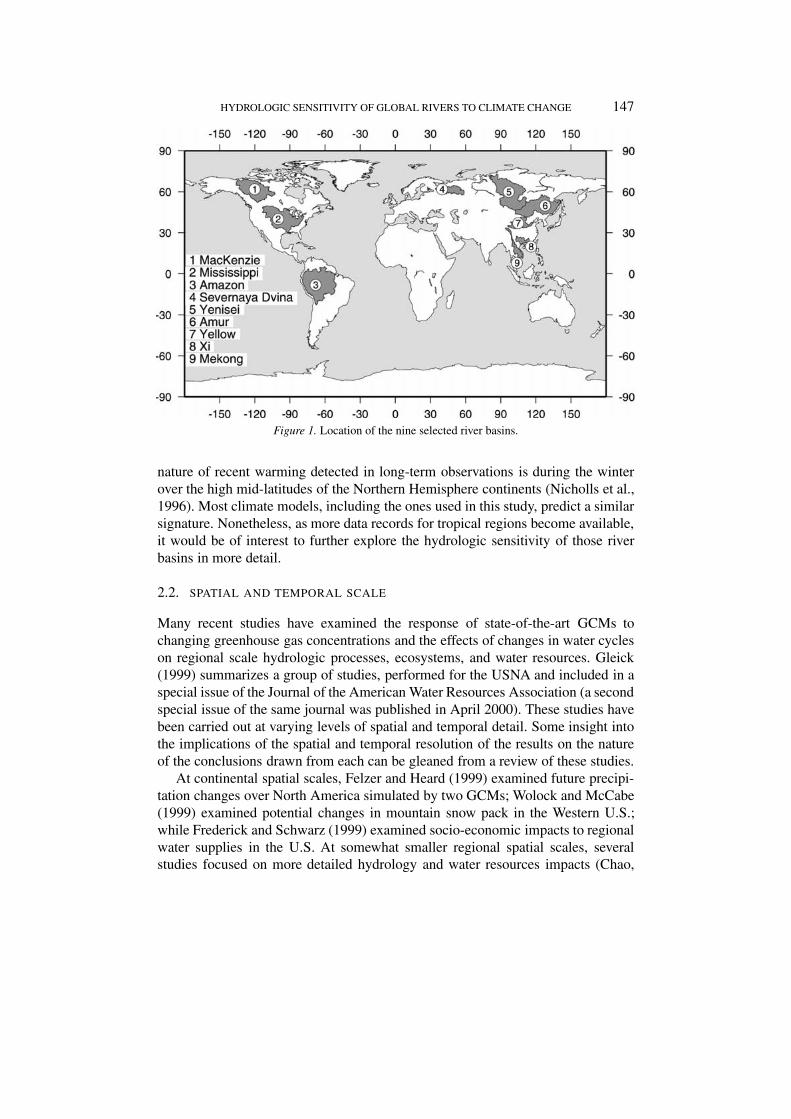
Given the large scale of application and the conceptual nature of some parame-terizations used in macroscale hydrological models (MHMs), some calibration ofmodel parameters is inevitably necessary (Nijssen et al., 2001a). However, thecalibration process is time-consuming and quickly becomes infeasible when themodeled area is large. To avoid this problem, Nijssen et al. (2001a) developed anapproach for transferring model parameters from calibrated to uncalibrated riverbasins. As part of their study, the variable infiltration capacity (VIC (Liang et al.,1994; Nijssen et al., 1997)) MHM was implemented for 26 large river basins. Theseriver basins were in turn a subset of the 50 continental-scale river basins delineatedby Graham et al. (1999). The nine river basins selected for this study (Table I) area subset of the 26 river basins studied by Nijssen et al. (2001a). They were selectedon the basis of the performance of the VIC model and the desire to represent arange of climatic and geographic regions globally. Figure 1 shows the location ofthe nine river basins. For each basin, historic river discharge records were obtainedfrom the Global River Discharge Center (GRDC) in Koblenz, Germany, and fromthe RivDis 1.1 data base (Vörösmarty et al., 1998).

Because of the paucity of data records in most of the tropics, the selected riverbasins are concentrated in the Northern Hemisphere. However, from a climatechange perspective this is not necessarily problematic. The most prominent sig-


Figure 1. Location of the nine selected river basins.

nature of recent warming detected in long-term observations is during the winterover the high mid-latitudes of the Northern Hemisphere continents (Nicholls et al.,1996). Most climate models, including the ones used in this study, predict a similarsignature. Nonetheless, as more data records for tropical regions become available,it would be of interest to further explore the hydrologic sensitivity of those riverbasins in more detail.

2.2. SPATIAL AND TEMPORAL SCALE

Many recent studies have examined the response of state-of-the-art GCMs tochanging greenhouse gas concentrations and the effects of changes in water cycleson regional scale hydrologic processes, ecosystems, and water resources. Gleick(1999) summarizes a group of studies, performed for the USNA and included in aspecial issue of the Journal of the American Water Resources Association (a secondspecial issue of the same journal was published in April 2000). These studies havebeen carried out at varying levels of spatial and temporal detail. Some insight intothe implications of the spatial and temporal resolution of the results on the natureof the conclusions drawn from each can be gleaned from a review of these studies.

At continental spatial scales, Felzer and Heard (1999) examined future precipi-tation changes over North America simulated by two GCMs; Wolock and McCabe(1999) examined potential changes in mountain snow pack in the Western U.S.;while Frederick and Schwarz (1999) examined socio-economic impacts to regionalwater supplies in the U.S. At somewhat smaller regional spatial scales, severalstudies focused on more detailed hydrology and water resources impacts (Chao,


1999; Gleick and Chalecki, 1999; Hamlet and Lettenmaier, 1999; Ojima et al.,1999; Olsen et al., 1999). At fine spatial scales, Leung and Wigmosta (1999), andMiller et al. (1999) examined watershed response based on downscaling of GCMsimulations using nested meso-scale climate models and high resolution distributedhydrology models for several small watersheds.

Each of these studies captures different climate and hydrologic effects. Largescale studies in some cases overlook seasonal or spatial distinctions that haveimportant consequences. For example, Frederick and Schwarz (1999) reported so-cioeconomic impacts to Pacific Northwest (PNW) water resources based on annualincreases in streamflow volumes. These impacts were almost certainly underesti-mated because reservoir storage in the Pacific Northwest is, in aggregate, muchless than mean annual runoff, meaning that it tends to be more sensitive to seasonalpatterns of runoff than to interannual variations. Frederick and Schwarz (1999)based their conclusions on predicted annual increases in streamflows, but did notconsider the large changes in the seasonal patterns of runoff that would occur underglobal warming. Hamlet and Lettenmaier (1999) and Leung and Wigmosta (1999),on the other hand, also predicted modest annual increases in streamflow for thePacific Northwest, but showed the importance of seasonal changes in streamflowpatterns and of topographic features such as basin elevation, which strongly affectthe timing of snowmelt, and hence runoff.

These results for the PNW suggest that studies of hydrologic sensitivity toclimate change should at the least include consideration of possible seasonal hy-drologic changes. Furthermore, the studies by Leung et al. (1999) and Hamletand Lettenmaier (1999) suggest that MHMs are able to capture the effects ofthe dominant climate signals for large river basins. Except in situations wherehigh-resolution, local interpretations of climatic sensitivities are required, MHMsshould be sufficient for regional impact studies. The selection of the spatial andtopographic scale of the modeling experiments described here are based on thispremise.

2.3. DOWNSCALING

Despite rapid advances in the development of GCMs, their output generally showssignificant biases in the simulation of both temperature and precipitation undercurrent climate conditions. These biases are often so large that direct applicationof the modeled meteorology in a macroscale hydrological model is not meaningful(e.g., Doherty and Mearns, 1999).

Various methods have been used to downscale GCM results to hydrologicallyrelevant spatial scales. One of the more appealing methods uses a nested regionalclimate model, which is forced at the boundary by the GCM, and which withinits domain resolves spatial scales relevant to the hydrological model. The problemwith this approach is that it is extremely computationally intensive and the resultsinherit biases not only from the global GCM, but also from the regional climate


model. The end result is invariably that the climate model output, downscaled ornot, must be adjusted so that a ‘base case’ scenario, intended to represent the cur-rent climate, does in fact have the same statistical characteristics as the historicalobservations. Adjustments are commonly required to create a base case, relativeto which alternative climate scenarios can be interpreted. A number of studieshave tested various downscaling methods ranging from very simple interpolations(e.g., Lettenmaier and Gan, 1990) to rather complicated methods that are basedon stochastic representation of the evolution of daily weather patterns, and theirrelationship to daily precipitation and temperature (Hughest et al., 1993).

The uncertainties of these past studies are based largely on the significant differ-ences in climate change predictions between the different GCMs. For the present,we therefore conclude that the simplest methods that impose the seasonal cycle ofregional-scale, GCM-predicted average changes on an observed temperature andprecipitation record are sufficient to investigate the range of hydrologic responses.Accordingly, predicted changes in precipitation and temperature were applied asa basin-wide, monthly average change. These changes were calculated as meanmonthly changes between a GCM control run and a particular decade in a transientGCM run. The CO2 (or equivalent greenhouse gas) concentration is kept constantin the control run (at historic levels in most cases) and is increased in the transientruns according to a specified emission scenario. Precipitation changes were definedas the relative change in aggregated precipitation volume over the basin, whiletemperature changes were defined as a shift in average temperature over the basin.

2.4. CLIMATE MODELS AND EMISSION SCENARIOS

Climate scenarios from eight different GCMs were obtained from the Inter-governmental Panel on Climate Change Data Distribution Center (IPCC DDC)(Table II). All eight models are coupled ocean-atmosphere models, output fromwhich was archived as part of the IPCC climate change efforts. Four of these mod-els (CCCMA-CGCM1, HCCPR-CM2, MPI-ECHAM4, and DOE-PCM3) werealso used as part of the U.S. National Assessment. The models differ in the spa-tial resolution and the processes they represent. Most of the models simulate achange in greenhouses gases by changing the CO2 concentration in the atmosphere,using an equivalent CO2 concentration, instead of explicit representation of theindividual greenhouse gases. Only two of the models (HCCPR-CM3 and DOE-PCM3) simulate the effects of a number of individual greenhouse gases explicitly.These two models are also the only two models that do not use a flux correction toaccount for biases in the energy and moisture fluxes between the atmosphere andocean. Four of the models use bucket-type land surface schemes to simulate landsurface hydrology, while the other four use more modern, explicit representationsof vegetation and incorporate more sophisticated runoff generation mechanisms.

The transient emission scenarios differ slightly between the models (Table II),partly because the models represent greenhouse gas chemistry differently. The


Table II

Selected climate models and scenarios

Organization Model Model Land Flux Transient Referenceresolution surface corrected? emissionlat. × lon. scheme scenario a

CCCMA CGCM1 3.75◦ × 3.75◦ Bucket Yes A Boer et al. (2000a,b)Canadian Centrefor ClimateModelling andAnalysis, Canada

CCSR CCSR 5.5◦ × 5.5◦ Bucket Yes B Emori et al. (1999)Center for Climate CGCMResearch Studies,Japan

CSIRO CSIRO 3.2◦ × 5.6◦ Bucket Yes B Gordon andCommonwealth CGCM O’FarrellScientific and (1997)Industrial ResearchOrganisation,Australia

GFDL GFDL 4.5◦ × 7.5◦ Bucket Yes A Manabe et al. (1991)Geophysical Fluid CGCM Stouffer andDynamics ManabeLaboratory, U.S.A. (1999)

HCCPR CM2 2.5◦ × 3.75◦ Vegetation Yes A Johns et al. (1997)Hadley Center for and runoffClimate Predictionand Research, U.K.

HCCPR CM3 2.5◦ × 3.75◦ Vegetation No C Gordon et al. (2000)Hadley Centre for and runoffClimate Predictionand Research, U.K.

MPI ECHAM4 2.8◦ × 2.8◦ Vegetation Yes B Röckner et al. (1996)Max Planck and runoff Röckner et al. (1999)Institute forMeteorology,Germany

DOE PCM3 2.8◦ × 2.8◦ Vegetation No C WashingtonDepartment of and runoff et al.Energy, U.S.A. (2000)

a The transient model scenarios are grouped as follows: A: 1% annual increase in equivalent CO2, and sulphate aerosols

according to IS92a; B: Equivalent CO2 and sulphate aerosols according to IS92a; C: Increase in several greenhouse gases and

sulphate aerosols according to IS92a.


three different emission scenarios used are: (a) 1% annual increase in equivalentCO2 and sulphate aerosols according to the IPCC IS92a scenario (A); (b) equiva-lent CO2 and sulphate aerosols according to IS92a (B); and (c) several greenhousegases (including CO2) and sulphate aerosols according to IS92a (C). The IS92ascenario is one of the emission scenarios specified by IPCC and gives a doublingof equivalent CO2 after about 95 years (IPCC, 1996). A 1% annual increase inequivalent CO2 (doubling in 70 years) results in a 20% higher radiative forcing fora given future time horizon compared to the IS92a scenario (IPCC, 1996).

Figure 2 shows the predicted changes in mean annual temperature and pre-cipitation for each of the nine basins for the decades 2020–2029, 2040–2049,and 2090–2099. These decades will hereafter be referred to as 2025, 2045, and2095, respectively. All models predict a progressive warming for all basins, but theamount of warming for each basin differs by model. Not unexpectedly, the spreadbetween the models increases with an increase in the lead time of the prediction.Some of the differences are likely attributable to the differences in the emission sce-narios, although there is no clear difference in warming signal between the modelsthat use scenario A and those that use scenarios B and C. Predicted annual averagewarming ranges from 0.8 ◦C for the Xi (HCCPR-CM2) to 4.2 ◦C for the Macken-zie (CCSR-CGCM) in 2025, from 1.1 ◦C for the Yenisei (DOE-PCM3) to 4.9 ◦Cfor the Mackenzie (CCSR-CGCM) in 2045, and from 2.5 ◦C for the Xi (DOE-PCM3) to 8.5 ◦C for the Mackenzie (CCSR-CGCM) in 2095. All models predictan increase of precipitation for the northern basins (Mackenzie, Severnaya Dvinaand Yenisei), but the signal is mixed for basins in the mid-latitudes and tropics,although on average slight precipitation increases are predicted. Predicted changesin precipitation range from –16.5% for the Xi (CCCMA-CGCM) to 15.0% for theMackenzie (CSIRO-CGCM) in 2025, from –15.9% for the Xi (CCCMA-CGCM)to 14.3% for the Severnaya Dvina (GFDL-CGCM) in 2045, and from –30.3% forthe Xi (CCCMA-CGCM) to 27.6% for the Mackenzie (CSIRO-CGCM) in 2095.The CCCMA-CGCM model generally predicts the largest decrease in precipitationand for many basins also the largest increase in temperature, especially in 2095.

In the remaining part of this study we will focus on the results of four of theclimate models (HCCPR-CM2, HCCPR-CM3, MPI-ECHAM4, and DOE-PCM3)and on two decades (2025 and 2045). These four models were selected becausethey offer the greatest spatial resolution, facilitating the downscaling step to the2◦ × 2◦ resolution of the hydrology models. More importantly, these four modelsinclude modern and relatively sophisticated land surface schemes that representexplicitly the interactions between vegetation and the surface energy and moisturebudgets. The decades 2025 and 2045 were selected for two reasons. First, in 2095the spread in the predicted changes in temperature and precipitation is much largerthan in the other two decades and some of the predicted changes in temperatureare very large, even for these four models (e.g., 7.0 ◦C warming for the Amazon in2095 (HCCPR-CM3)). Second, planning horizons in water resources development


Figure 2. Predicted changes in mean annual temperature and precipitation for each river basinfor the decades 2020–2029 (2025), 2040–2049 (2045), and 2090–2099 (2095). Note that climateprediction for 2095 were not available for GFDL-CGCM and MPI-ECHAM4. Also note that theCCCMA-CGCM model provided three ensemble runs, all three of which are plotted.

are more typically on the order of 20–30 years, placing a greater emphasis on thedecades 2025 and 2045.

2.5. VARIABLE INFILTRATION CAPACITY MODEL

The predicted changes in temperature and precipitation, that is, the mean monthlydifferences between the GCM transient and control runs, were used to perturb ob-served temperature and precipitation records. Both the historical and the perturbedrecords were used to drive a MHM to study the hydrological effects of changesin atmospheric forcings. The MHM used in this study is the variable infiltrationcapacity (VIC) model (e.g., Liang et al., 1994, 1996; Nijssen et al., 1997). The


VIC MHM has been used in a number of modeling studies of large river basins(e.g., Abdulla et al., 1996; Cherkauer and Lettenmaier, 1999; Lohmann et al.,1998b; Matheussen et al., 2000; Nijssen et al., 1997, 2001a,b; Wood et al., 1997).Distinguishing characteristics of the VIC model include the representation of:

• subgrid variability in land surface vegetation classes;• subgrid variability in the soil moisture storage capacity, which is represented

as a spatial probability distribution;• subgrid variability in topography through the use of elevation bands;• drainage from the lower soil moisture zone (baseflow) as a nonlinear reces-

sion;• spatial subgrid variability in precipitation.

The VIC model calculates the moisture fluxes for each model grid cell inde-pendently. Because the model grid cells are large (2◦ × 2◦), it is assumed thatthere is no significant exchange of ground water between the cells. The generateddaily baseflow and ‘fast response’ runoff are routed downstream using a stand-alone routing model, which is described in detail by Lohmann et al. (1996, 1998a).Streamflow can exit each grid cell in eight directions and all flow must exit in thesame direction. The flow from each grid cell is weighted by the fraction of the gridcell that lies within the basin. As in Nijssen et al. (2001a,b) flows were routed on a1◦ × 1◦ network, because the higher resolution flow networks allowed a somewhatbetter approximation of the modeled channel network than the native 2◦×2◦ spatialresolution.

In the context of the climate change simulations it should be noted that theVIC model does not include CO2 enrichment effects. Although the direct effectsof increased temperatures and CO2 concentrations on plant growth are reasonablywell understood individually, their combined outcome is unclear and merits morestudy (Kirschbaum et al., 1996; Melillo et al., 1996). Similarly, climate-inducedvegetation changes were not considered in the model experiments, and all modelruns were executed using the baseline vegetation.

2.6. BASELINE SIMULATION

The baseline simulation acts as a surrogate for the real system under current climateconditions. In the baseline simulation the VIC model was forced with observedtemperature and precipitation. This allowed a comparison between modeled andobserved hydrographs to ensure that the MHM can capture and replicate the impor-tant hydrological processes. Subsequently, all changes in hydrological fluxes andstorages were calculated relative to this baseline simulation. Results from previouswork by Nijssen et al. (2001a,b) were used for the baseline simulations.

In Nijssen et al. (2001b), a gridded data set of daily meteorological modelforcings for the period 1979–1993 was developed for global land areas (excludingGreenland and Antarctica) at a spatial resolution of 2◦ ×2◦. Daily precipitation and


daily minimum and maximum temperature were derived from station observations,and extended using stochastic interpolation methods for those areas with insuf-ficient coverage by daily meteorological stations. The resulting daily sequenceswere scaled to match the means of pre-existing global, monthly time series (Hulme,1995; Huffman et al., 1997; Jones, 1994). Daily surface wind speeds were obtainedfrom the NCEP/NCAR reanalysis project (Kalnay et al., 1996). The remainingmeteorological forcings (vapor pressure, incoming shortwave radiation, and netlongwave radiation) are calculated by the VIC model based on daily temperatureand precipitation using algorithms by Kimball et al. (1997), Thornton and Running(1999), and Bras (1990).

The daily data were used to drive the VIC model to calculate a set of derivedvariables (evapotranspiration, runoff, snow water equivalent, and soil moisture) andto study the water balance of each of the continents. For each 2◦×2◦ model grid cellland surface characteristics such as elevation, soil and vegetation were specified.Elevation data were calculated based on the 5 minute TerrainBase Digital ElevationModel (DEM) (Row et al., 1995), using the land surface mask from Graham et al.(1999). Vegetation types were provided by the AVHRR-based, 1 km, global landclassification from Hansen et al. (2000), which has 12 unique vegetation classes.Vegetation parameters such as height and minimum stomatal resistance were as-signed to each individual vegetation class. Soil textural information and soil bulkdensities were derived from the five minute FAO-UNESCO digital soil map of theworld (FAO, 1995), combined with the WISE pedon data base (Batjes, 1995). Theremaining soil characteristics, such as porosity, saturated hydraulic conductivity,and the exponent for the unsaturated hydraulic conductivity equation were basedon Cosby et al. (1984).

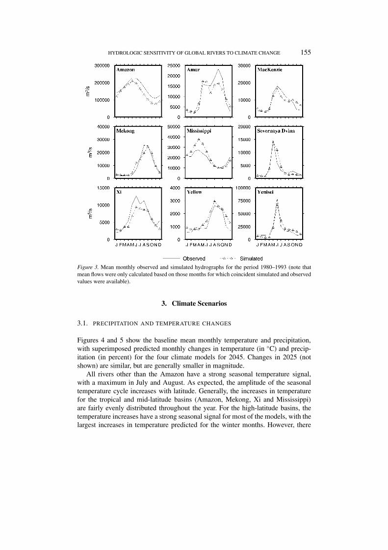
As discussed in Section 2.1, Nijssen et al. (2001a) used the same (base case)data and model to evaluate methods for model parameter transfer from calibrated touncalibrated basins. The final calibrated flows for the nine selected basins (whichwere taken from Nijssen et al. (2001a)) had a mean absolute bias in the annualflow volume of 10.0% and a mean relative root mean squared error of the monthlydischarge time series of 40.6%. The mean monthly hydrographs of observed andsimulated flow are shown in Figure 3. We again emphasize that in the remainderof this paper, when examining the hydrologic effects of altered climate scenarios,the change in the hydrologic fluxes were calculated relative to the results from thebaseline simulation, rather than the historic observations. This convention avoids,at least to first order, the effects of model bias.


Figure 3. Mean monthly observed and simulated hydrographs for the period 1980–1993 (note thatmean flows were only calculated based on those months for which coincident simulated and observedvalues were available).

3. Climate Scenarios

3.1. PRECIPITATION AND TEMPERATURE CHANGES

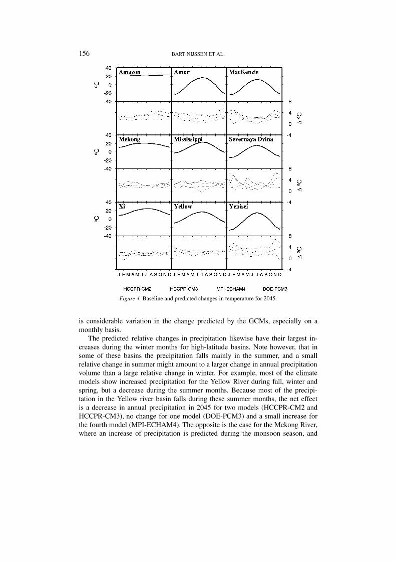
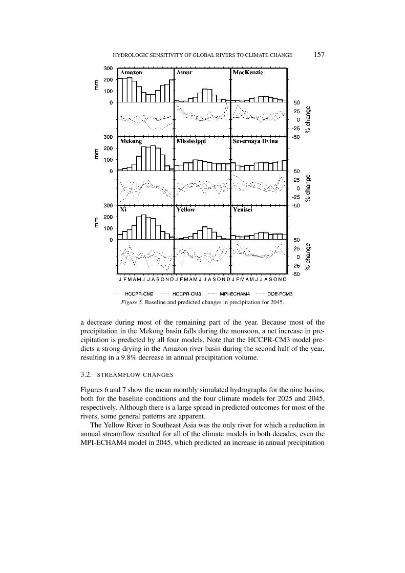
Figures 4 and 5 show the baseline mean monthly temperature and precipitation,with superimposed predicted monthly changes in temperature (in ◦C) and precip-itation (in percent) for the four climate models for 2045. Changes in 2025 (notshown) are similar, but are generally smaller in magnitude.

All rivers other than the Amazon have a strong seasonal temperature signal,with a maximum in July and August. As expected, the amplitude of the seasonaltemperature cycle increases with latitude. Generally, the increases in temperaturefor the tropical and mid-latitude basins (Amazon, Mekong, Xi and Mississippi)are fairly evenly distributed throughout the year. For the high-latitude basins, thetemperature increases have a strong seasonal signal for most of the models, with thelargest increases in temperature predicted for the winter months. However, there


Figure 4. Baseline and predicted changes in temperature for 2045.

is considerable variation in the change predicted by the GCMs, especially on amonthly basis.

The predicted relative changes in precipitation likewise have their largest in-creases during the winter months for high-latitude basins. Note however, that insome of these basins the precipitation falls mainly in the summer, and a smallrelative change in summer might amount to a larger change in annual precipitationvolume than a large relative change in winter. For example, most of the climatemodels show increased precipitation for the Yellow River during fall, winter andspring, but a decrease during the summer months. Because most of the precipi-tation in the Yellow river basin falls during these summer months, the net effectis a decrease in annual precipitation in 2045 for two models (HCCPR-CM2 andHCCPR-CM3), no change for one model (DOE-PCM3) and a small increase forthe fourth model (MPI-ECHAM4). The opposite is the case for the Mekong River,where an increase of precipitation is predicted during the monsoon season, and


Figure 5. Baseline and predicted changes in precipitation for 2045.

a decrease during most of the remaining part of the year. Because most of theprecipitation in the Mekong basin falls during the monsoon, a net increase in pre-cipitation is predicted by all four models. Note that the HCCPR-CM3 model pre-dicts a strong drying in the Amazon river basin during the second half of the year,resulting in a 9.8% decrease in annual precipitation volume.

3.2. STREAMFLOW CHANGES

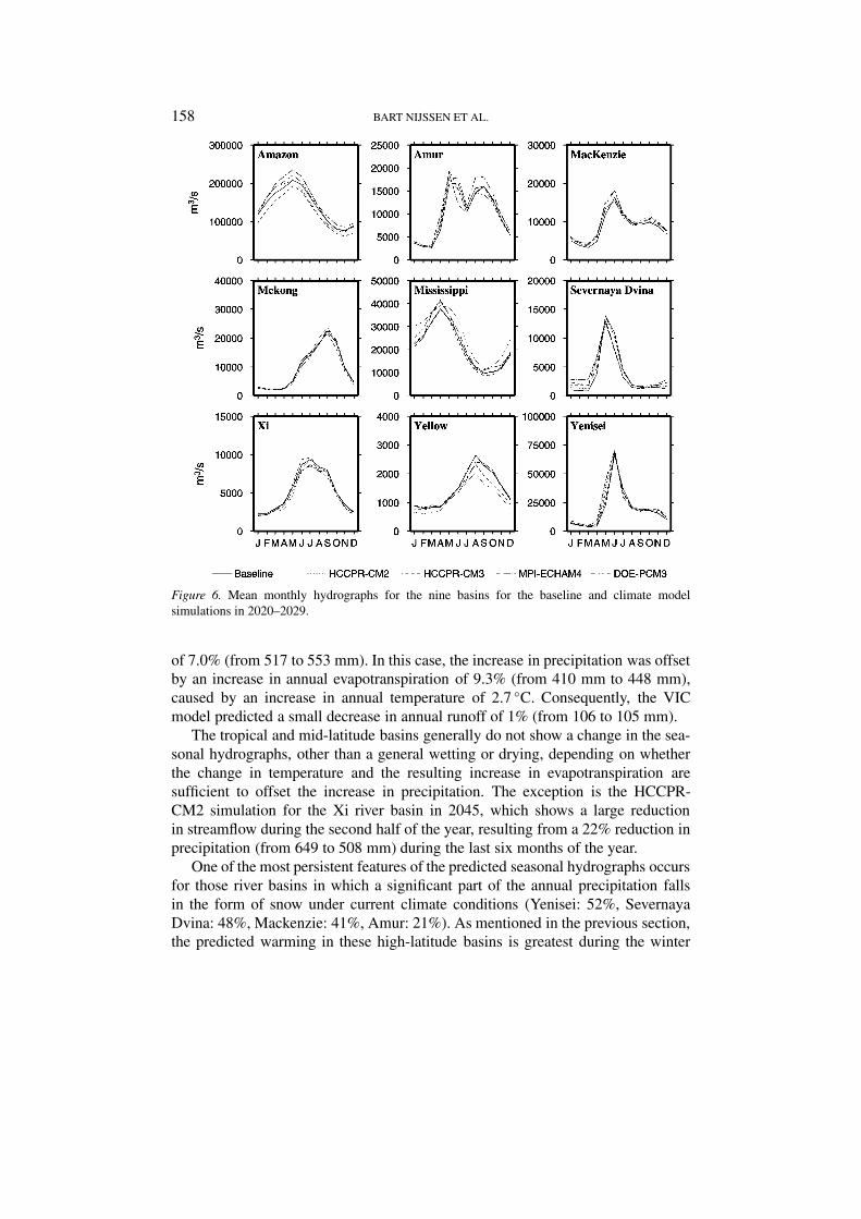
Figures 6 and 7 show the mean monthly simulated hydrographs for the nine basins,both for the baseline conditions and the four climate models for 2025 and 2045,respectively. Although there is a large spread in predicted outcomes for most of therivers, some general patterns are apparent.

The Yellow River in Southeast Asia was the only river for which a reduction inannual streamflow resulted for all of the climate models in both decades, even theMPI-ECHAM4 model in 2045, which predicted an increase in annual precipitation


Figure 6. Mean monthly hydrographs for the nine basins for the baseline and climate modelsimulations in 2020–2029.

of 7.0% (from 517 to 553 mm). In this case, the increase in precipitation was offsetby an increase in annual evapotranspiration of 9.3% (from 410 mm to 448 mm),caused by an increase in annual temperature of 2.7 ◦C. Consequently, the VICmodel predicted a small decrease in annual runoff of 1% (from 106 to 105 mm).

The tropical and mid-latitude basins generally do not show a change in the sea-sonal hydrographs, other than a general wetting or drying, depending on whetherthe change in temperature and the resulting increase in evapotranspiration aresufficient to offset the increase in precipitation. The exception is the HCCPR-CM2 simulation for the Xi river basin in 2045, which shows a large reductionin streamflow during the second half of the year, resulting from a 22% reduction inprecipitation (from 649 to 508 mm) during the last six months of the year.

One of the most persistent features of the predicted seasonal hydrographs occursfor those river basins in which a significant part of the annual precipitation fallsin the form of snow under current climate conditions (Yenisei: 52%, SevernayaDvina: 48%, Mackenzie: 41%, Amur: 21%). As mentioned in the previous section,the predicted warming in these high-latitude basins is greatest during the winter


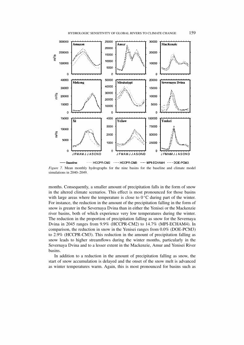
Figure 7. Mean monthly hydrographs for the nine basins for the baseline and climate modelsimulations in 2040–2049.

months. Consequently, a smaller amount of precipitation falls in the form of snowin the altered climate scenarios. This effect is most pronounced for those basinswith large areas where the temperature is close to 0 ◦C during part of the winter.For instance, the reduction in the amount of the precipitation falling in the form ofsnow is greater in the Severnaya Dvina than in either the Yenisei or the Mackenzieriver basins, both of which experience very low temperatures during the winter.The reduction in the proportion of precipitation falling as snow for the SevernayaDvina in 2045 ranges from 9.9% (HCCPR-CM2) to 14.7% (MPI-ECHAM4). Incomparison, the reduction in snow in the Yenisei ranges from 0.0% (DOE-PCM3)to 2.9% (HCCPR-CM3). This reduction in the amount of precipitation falling assnow leads to higher streamflows during the winter months, particularly in theSevernaya Dvina and to a lesser extent in the Mackenzie, Amur and Yenisei Riverbasins.

In addition to a reduction in the amount of precipitation falling as snow, thestart of snow accumulation is delayed and the onset of the snow melt is advancedas winter temperatures warm. Again, this is most pronounced for basins such as


the Severnaya Dvina, where temperatures are not as cold as in the Yenisei orMackenzie basins. For all basins where a significant part of the precipitation isstored as snow during the winter months, the hydrographs increase earlier in thespring under the altered climate scenarios. However, the warmer basins, such asthe Severnaya Dvina, show a decrease in the spring peak flows despite an increasein winter precipitation as a result of shallower snow packs. The cold basins onthe other hand show an increase in the spring peak flows, because almost all ofthe increase in winter precipitation is stored as snow during the winter months.Maximum basin-wide snow accumulation in the Severnaya Dvina decreases from313 mm water equivalent in April under current climate conditions to maximumaccumulation in 2045 ranging from 164 mm in March (MPI-ECHAM4) to 264 mmin March (DOE-PCM3). In contrast, maximum accumulation in the Yenisei riverbasin increases from 210 mm in April under current conditions to maximum ac-cumulation in 2045 ranging from 217 mm in April (HCCPR-CM3) to 237 mm inApril (MPI-ECHAM4). Mid-latitude basins (Mississippi and Yellow) also show asignificant decrease in the amount of precipitation falling as snow.

3.3. WATER BALANCE CHANGES

The monthly water balance for a river basin is given by

Pt = Et + Rt + �St , (1)

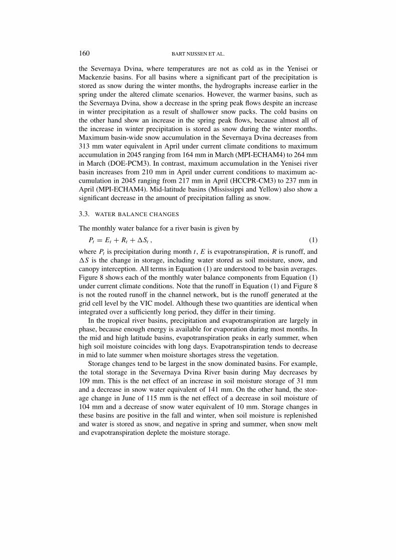
where Pt is precipitation during month t , E is evapotranspiration, R is runoff, and�S is the change in storage, including water stored as soil moisture, snow, andcanopy interception. All terms in Equation (1) are understood to be basin averages.Figure 8 shows each of the monthly water balance components from Equation (1)under current climate conditions. Note that the runoff in Equation (1) and Figure 8is not the routed runoff in the channel network, but is the runoff generated at thegrid cell level by the VIC model. Although these two quantities are identical whenintegrated over a sufficiently long period, they differ in their timing.

In the tropical river basins, precipitation and evapotranspiration are largely inphase, because enough energy is available for evaporation during most months. Inthe mid and high latitude basins, evapotranspiration peaks in early summer, whenhigh soil moisture coincides with long days. Evapotranspiration tends to decreasein mid to late summer when moisture shortages stress the vegetation.

Storage changes tend to be largest in the snow dominated basins. For example,the total storage in the Severnaya Dvina River basin during May decreases by109 mm. This is the net effect of an increase in soil moisture storage of 31 mmand a decrease in snow water equivalent of 141 mm. On the other hand, the stor-age change in June of 115 mm is the net effect of a decrease in soil moisture of104 mm and a decrease of snow water equivalent of 10 mm. Storage changes inthese basins are positive in the fall and winter, when soil moisture is replenishedand water is stored as snow, and negative in spring and summer, when snow meltand evapotranspiration deplete the moisture storage.


Figure 8. Mean monthly water balance components for current climate conditions for the nine riverbasins. Averages are for the period 1980–1993.

Figure 9 shows the change in the mean monthly water balance components forthe DOE-PCM3 scenario in 2045. The DOE-PCM3 scenario was selected, becausethe associated hydrographs are generally representative of the changes predictedby the other models (see Figures 6 and 7). Temperature changes from the DOE-PCM3 model tend to be somewhat smaller than for the other models, with annualbasinwide temperature changes in 2045 ranging from 1.1 ◦C for the Yenisei to1.9 ◦C for the Mackenzie. Annual precipitation changes in 2045 range from –0.8%for the Xi to 7.7% for the Amur River basin.

In the Amazon basin a positive change in both precipitation and temperature istranslated into an increase in evapotranspiration and runoff in most months. TheMekong and the Xi river basins, both in Southeast Asia, exhibit an increase ofprecipitation during the early part of the monsoon season and a decrease during thelast part of the monsoon and during the dry season. Both runoff and evaporationare increased during most months with increased precipitation. However, much ofthe increased precipitation during the early part of the monsoon season is used to


Figure 9. Predicted changes in the monthly water balance components in 2045 for the DOE-PCM3scenario.

replenish soil moisture storage. Changes in the amount of water that enters or isreleased from soil moisture storage are particularly large in the Xi basin, whichaccording to the DOE-PCM3 model, will experience the largest absolute changesin precipitation (increase of 39 mm in August and a decrease of 22 mm in bothOctober and November).

Among the snow-dominated basins, the coldest basins again show a differentsignal as compared to the warmer basins. For the coldest basins (Amur, Macken-zie, and Yenisei) an increase in moisture storage is predicted during the wintermonths, because most of the increased precipitation is stored as snow. Conse-quently, snowmelt runoff is increased. In the warmer basins (Severnaya Dvina andMississippi) snow water storage decreases, resulting in increased runoff during thewinter, but decreased runoff during the snowmelt period.


4. Sensitivity Study

Diagnosis of the results presented in the previous section provides insight into thecauses of changes in the hydrographs associated with the four different climatemodels. Nonetheless, it is difficult to analyze the hydrologic processes that areresponsible for some of the changes in the water balance components, both becausethe climate models predict simultaneous changes in precipitation and temperature,and because there can be large month-to-month variations in the changes (even intheir direction).

To isolate processes that lead to changes in the water balance components, weperformed a controlled model experiment, in which temperature and precipitationwere increased by fixed amounts for specified periods. Temperature was increasedby 2 ◦C during each of the four seasons, here defined as December–February (DJF),March–May (MAM), June–August (JJA), and September–November (SON). Sep-arately, the precipitation was increased by 10% during each of these four seasonsas well. The results of this sensitivity experiment provide the basis for theinterpretations in the following two sections.

4.1. SEASONAL CHANGE IN TEMPERATURE

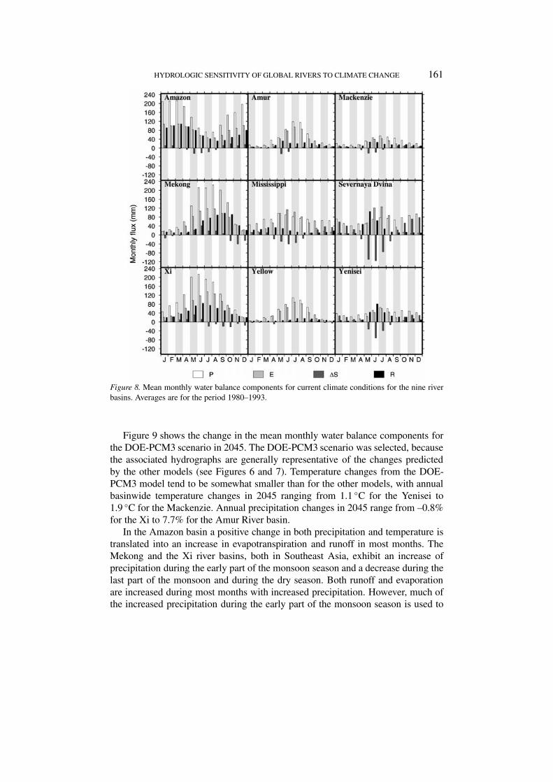
Figure 10 shows the change in seasonal evapotranspiration in response to anincrease in mean monthly temperature of 2 ◦C. The seasons along the abscissarepresent the seasons during which the change in temperature was imposed, whilethe seasons along the ordinate axis correspond to the seasons for which the result-ing change in the evapotranspiration was calculated. Thus, in Figure 10, circlesalong the diagonal represent changes in evapotranspiration during the same seasonin which the change in temperature was imposed. Off diagonal circles representchanges in season Y due to a change in temperature in season X. The area of thecircles represents the magnitude of the relative change in the evapotranspiration,with black representing an increase and gray a decrease in evapotranspiration.Similarly, Figure 11 shows the relative change in runoff resulting from the sameincrease in temperature. Note that the circles represent percentage changes relativeto the base case and that the scale of the circles is the same in both Figures 10 and11.

For example, the panels for the Severnaya Dvina indicate that a 2◦ increase intemperature in the winter (DJF), leads to an increase in winter evapotranspiration ofmore than 10%, followed by a small increase in spring (MAM) evapotranspiration(Figure 10). The same temperature increase in the fall (SON) leads to an increase infall runoff, but to an even greater relative increase in winter runoff (Figure 11). Incontrast, a temperature increase in the summer (JJA) results in a decrease in runoffin all seasons for this basin (Figure 11).

The black circles on the main diagonal in Figure 10 indicate that an increase intemperature leads to an increase in evapotranspiration in the season in which the


Figure 10. Relative change in seasonal evapotranspiration due to an increase in mean monthly tem-perature of 2 ◦C. The seasons along the abscissa represent the seasons during which the change intemperature was imposed, while the seasons along the ordinate axis correspond to the seasons forwhich the resulting change in the evapotranspiration was calculated. The magnitude of the relativechange is indicated by the area of the circle, with black representing an increase and gray a decreasein evapotranspiration (see text for details).

temperature is increased. Note that because the circles represent relative changes,the large changes during the winter in the cold climates represent only a smallabsolute increase in evapotranspiration. In most cases the increase in evapotranspi-ration during the months in which the temperature is increased is accompanied bya decrease in evapotranspiration during the remaining months, because without asimultaneous increase in precipitation less water remains in storage and moisturestress is increased. This effect is strongest in the season immediately followingthe season in which the temperature change is imposed, and generally decreasesfor the seasons after that. The only exception to this is in the Severnaya Dvinabasin, where an increase in temperature during the fall (SON) or winter (DJF)


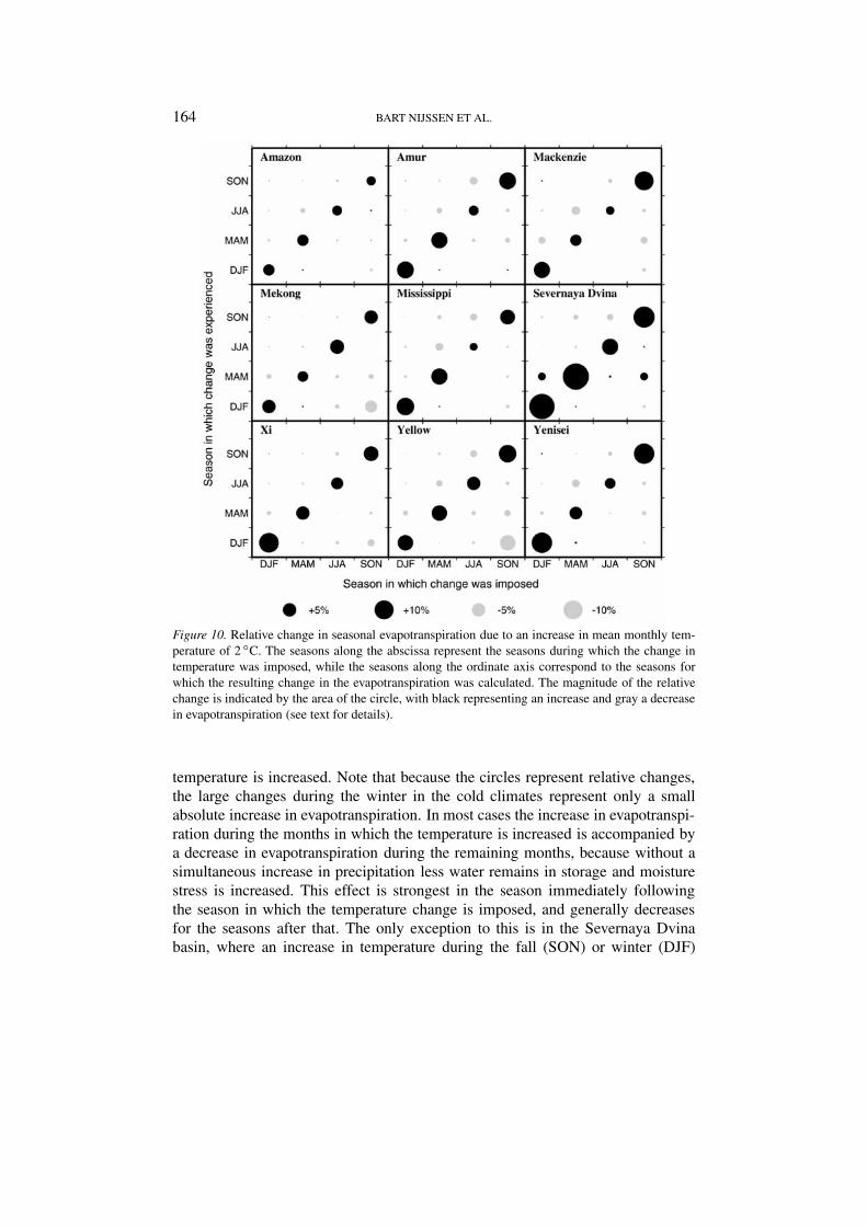
Figure 11. Relative change in seasonal runoff due to an increase in mean monthly temperature of2 ◦C. For details see Figure 10 and the text.

leads to an increase in evapotranspiration during the spring (MAM) as well. In thiscase, a larger proportion of the precipitation in the fall and winter falls as rain,leading to reduction in the depth of the snow pack. In turn, the number of snowfree days in May (defined as the area-weighted sum of snow free days per gridcell), increases by about one day. This leads to an increase in transpiration of about1.5 mm (in the VIC model the vegetation does not transpire when snow is on theground or in the canopy). Some of the basins also show a very small increase inevapotranspiration during the season preceding the season in which the temperatureincrease was imposed. These changes do not appear to be significant, because inall cases their magnitude is much less than 1 mm over a period of three months.

Figure 11 shows that increases in temperature generally lead to decreases inrunoff, commensurate with the increases in evapotranspiration shown in Figure 10.The only cases where an increase in temperature leads to an increase in runoffis during the winter and spring months in those basins where water stored as


snow forms a significant component of the water balance. In the coldest basins(Yenisei, Mackenzie, and Amur) the greatest change occurs during MAM, becausethe temperature during DJF remains well below 0 ◦C, even with an increase of2 ◦C. In contrast, the change in runoff in the Severnaya Dvina basin is more evenlydistributed over the fall, winter and spring months.

4.2. SEASONAL CHANGE IN PRECIPITATION

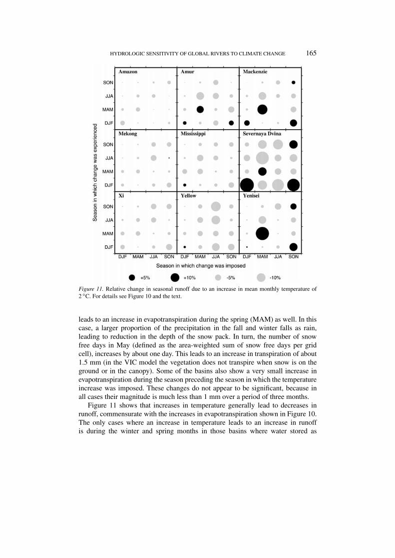
Increasing precipitation increases both evapotranspiration (Figure 12) and runoff(Figure 13). Relative changes in runoff are generally larger than relative changes inevapotranspiration. To some extent, this can be explained because runoff forms asmaller component of the water balance than evapotranspiration, and an increase inboth of 10 mm will result in a greater relative change in runoff. However, becausethe relative changes are different, the relative importance of runoff in the waterbalance increases. Because evapotranspiration is energy-limited during the wintermonths in the snow dominated basins, evapotranspiration in the winter increasesonly slightly in response to increases in precipitation during that period. Theevapotranspiration in those basins responds much more strongly in summer, whensufficient energy is available to evaporate much of the extra precipitation. In thecoldest basins the runoff change resulting from a winter increase in precipitation islargest in spring and summer, because most of the winter precipitation is stored assnow.

In the Severnaya Dvina river basin evapotranspiration decreases in the seasonafter increasing the precipitation. In particular, evapotranspiration during the springdecreases, following an increase in precipitation during the fall and winter. Themechanism is the same as described in the previous section. Increased precipitationduring the fall or winter leads to a thicker snow pack and reduces the number ofsnow free days during the spring, resulting in a small reduction of total evaporationduring these three months.

4.3. OBSERVED TRENDS IN STREAMFLOW

Lins and Slack (1999), in a study of streamflow trends in the United States dur-ing the period 1944–1993, noted that trends were most prevalent in the annualminimum to median flows and least prevalent in the annual maximum category.Generally, increases in streamflow were observed across most of the United States,except in the Southeast and the Pacific Northwest, where decreases were observed.They concluded that the conterminous United States is becoming wetter and lessextreme. Gan (1998) in a study of the Canadian Prairies, found that over the last40–50 years many stations observed positive trends in streamflow during March,attributed to an earlier onset of snowmelt, followed by lower flows in May and june.This shift in streamflow is similar to the response of the Mackenzie and SevernayaDvina we predict for an increase in temperature during the winter months (Fig-ure 11). Similarly, Grabs et al. (2000) found a positive trend in the annual discharge


Figure 12. Relative change in seasonal evapotranspiration due to an increase in mean monthlyprecipitation of 10%. For details see Figure 10 and the text.

time series of Siberian rivers, with negative trends in the summer, and a positivetrend during winter and early spring. Those observed trends are likewise similarto the signature we predict for warmer winter temperatures. Analysis of the annualstreamflow of large rivers in southeastern South America for the period 1911–1993(Robertson and Mechoso, 1998), showed an upward trend in the Paraguay-Paraná,especially since about 1960. The same trend was observed by Genta et al. (1998),who also noted that the amplitude of the seasonal cycle had decreased. Marengoet al. (1998) showed that variations in streamflow in Amazonia were stronglyrelated to El Niño, but found no significant trends to wetter or drier conditions.The observed changes in South American rivers are consistent with our results inthat changes in precipitation have an immediate and strong effect on streamflow(Figure 13).


Figure 13. Relative change in seasonal runoff due to an increase in mean monthly precipitation of10%. For details see Figure 10 and the text.

5. Changes in Drought Statistics

Because existing water resource management systems and ecosystems have de-veloped to cope with current streamflow rates and volumes (and their variability),both increases and decreases in streamflow can have adverse effects. Increases inthe length and intensity of droughts are of particular concern, because of globallyincreasing water supply demands (e.g., Vörösmarty et al., 2000). Floods, whichare relatively short-term phenomena, are difficult to represent adequately given themonthly timestep of the flow data available to us. In addition, a different type ofstudy would be required to examine the effects of changes in extreme precipitation,which are often the cause of floods.

A metric that can be used to assess the hydrologic vulnerability of a river basinis the average deficit length (L), that is, the average number of consecutive yearsthat the annual river discharge is unable to meet a certain demand level (D). In


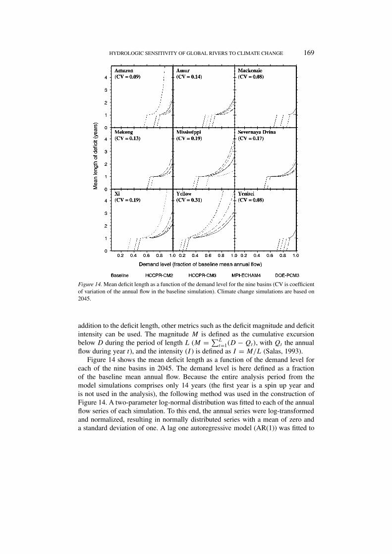
Figure 14. Mean deficit length as a function of the demand level for the nine basins (CV is coefficientof variation of the annual flow in the baseline simulation). Climate change simulations are based on2045.

addition to the deficit length, other metrics such as the deficit magnitude and deficitintensity can be used. The magnitude M is defined as the cumulative excursionbelow D during the period of length L (M = ∑L

t=1(D − Qt), with Qt the annualflow during year t), and the intensity (I ) is defined as I = M/L (Salas, 1993).

Figure 14 shows the mean deficit length as a function of the demand level foreach of the nine basins in 2045. The demand level is here defined as a fractionof the baseline mean annual flow. Because the entire analysis period from themodel simulations comprises only 14 years (the first year is a spin up year andis not used in the analysis), the following method was used in the construction ofFigure 14. A two-parameter log-normal distribution was fitted to each of the annualflow series of each simulation. To this end, the annual series were log-transformedand normalized, resulting in normally distributed series with a mean of zero anda standard deviation of one. A lag one autoregressive model (AR(1)) was fitted to


each of the annual series, and a 10,000 year series of annual flows was generatedusing the AR(1) model (Salas, 1993). These 10,000 year time series were then usedto calculate the mean deficit lengths plotted in Figure 14. The demand level wasdefined as a fraction of the baseline mean annual flow and increased in steps of 5%between 5% and 100% of the baseline mean annual flow.

Arguably, a 14 year time series will in most cases be insufficient to fit an AR(1)model and derive reliable statistics. However, in this case we are concerned witha change in the mean deficit length as a function of a change in climate, in orderto evaluate the change in vulnerability of the different basins. Because we are onlyinterested in changes relative to the base case, we argue that even though the actualnumbers may be open to discussion, the qualitative changes in the vulnerabilityreflected by the curves in Figure 14 are informative.

The range of the baseline curves in Figure 14 reflects the coefficient of varia-tion (CV) of the annual flows (the coefficient of variation of a statistical sampleis defined as the standard deviation divided by the mean). The arctic rivers andthe Amazon have the lowest CV (Mackenzie and Yenisei: CV = 0.08, Amazon:CV = 0.09), while the Yellow shows the highest CV (CV = 0.31).

An upward shift of the curves in Figure 14 reflects a drying of the basin, becausethe average deficit length increases for the same demand level. A downward shiftscorresponds to a decrease of the average deficit length for a given demand level,and consequently represents a wetting of the basin. As seen before, all modelspredict a drying in the Yellow River basin in 2045, with the largest degree ofdrying predicted by the two Hadley Centre models. The Xi also becomes drier, withonly one model (HCCPR-CM2) predicting a large change. Two models predict anincrease in runoff in the Amazon, one predicts a slight decrease, while the HCCPR-CM3 model predicts a large increase in the mean deficit length. The high latitudebasins generally become wetter. For these basins, the increase in temperature dur-ing the winter months contributes only slightly to an increase in evapotranspiration,and much of the increased precipitation consequently contributes to an increase inrunoff. The signals for the Mekong and Mississippi are mixed.

Figure 14 shows the extent of disagreement in the regional simulations that stillexists between the various GCMs. Whereas HCCPR-CM2 predicts the greatestdrying in the Amazon and MPI-ECHAM4 predicts the greatest wetting, this signalis reversed in the Mississippi, where MPI-ECHAM4 predicts the greatest wettingand HCCPR-CM2 the greatest drying.

6. Conclusions

Transient climate predictions from four GCMs were used to assess the hydrologicsensitivity to climate change of nine large, continental river basins. The GCMswere selected because they have modern land surface schemes, high spatial reso-lutions, and generally represent the current state-of-the-art in climate simulations.


All of the models used either the IPCC IS92a emission scenario, or a 1% compoundannual increase in CO2. The nine river basins represent a range of geographic andclimatic conditions. Changes in basinwide, mean annual temperature and precipi-tation were calculated for three decades in the transient climate model runs (2025,2045, and 2095) and hydrologic model simulations were performed for decadescentered on 2025 and 2045. In addition, sensitivity analyses were performed inwhich temperature and precipitation were increased independently by 2 ◦C and10%, respectively, during each of four seasons.

The main conclusions of this study are:

• All models predict a warming for all nine basins, but the amount of warmingvaries widely between the models, especially with increased time horizon. Thegreatest warming is predicted to occur during the winter months in the high-est latitudes. Precipitation generally increases, but the monthly precipitationsignal varies more between the models than does temperature.

• The largest changes in the hydrological cycle are predicted for the snow-dominated basins of mid to higher latitudes. Partly, this is a result of thegreater amount of warming that is predicted for these regions. More im-portantly, though, the presence or absence of snow fundamentally changesthe nature of the land surface water balance, because of the effect of waterstorage in the snow pack. Water stored as snow during the winter does notbecome available for runoff or evapotranspiration until the following spring’smelt period. Because of this cumulative process, the snow pack integrates theeffects of climate change over a period of months, and the largest hydrologicalchanges are manifested in the early to mid spring melt period. In general,the streamflow regime in snowmelt dominated basins is most sensitive toincreases in temperature during the winter months.

• Somewhat different sensitivities to climate warming are predicted for thecoldest snow dominated basins than for transitional basins. Whereas the for-mer show an increase of the spring streamflow peak in response to warmertemperatures and increased winter precipitation, the latter show a decrease. Inthe coldest basins, any increase in precipitation during the winter is stored assnow, because even for a relatively large increase in temperature, winters willremain quite cold with temperatures generally well below freezing. In con-trast, in the warmer basins increased temperature leads to increased rainfallduring the winter and a decrease in the depth of the snow pack. The net effectis that the spring snow melt peak is reduced.

• Globally, the hydrological response predicted for most of the basins in re-sponse to the GCMs predictions is a reduction in annual streamflow in thetropical and mid-latitudes. In contrast, high-latitude basins tend to show anincrease in annual runoff, because most of the predicted increase in precipita-tion occurs during the winter, when the available energy is insufficient for an


increase in evaporation. Instead, water is stored as snow and contributes to anincrease in streamflow during the following snow melt period.

Acknowledgement

This work was supported by the U.S. Environmental Protection Agency underSTAR Grant R 824802-01-0 to the University of Washington.

References

Abdulla, F. A., Lettenmaier, D. P., Wood, E. F., and Smith, J. A.: 1996, ‘Application of a MacroscaleHydrologic Model to Estimate the Water Balance of the Arkansas-Red River Basin’, J. Geophys.Res. 101, 7449–7459.

Arnell, N. W.: 1999a, ‘The Effect of Climate Change on Hydrological Regimes in Europe: AContinental Perspective’, Global Environ. Change 9, 5–23.

Arnell, N. W.: 1999b, ‘Climate Change and Global Water Resources’, Global Environ. Change 9,S31–S49.

Batjes, N. H.: 1995, A Homogenized Soil Data File for Global Environmental Research: A Subset ofFAO, ISRIC and NCRS Profiles, Technical Report, International Soil Reference and InformationCentre (ISRIC), Wageningen.

Battisti, D. and Sarachik, E.: 1995, ‘Understanding and Predicting ENSO’, Rev. Geophys. 33, 1367–1376.

Boer, G. J., Flato, G., and Ramsden, D.: 2000a, ‘A Transient Climate Change Simulation with Green-house Gas and Aerosol Forcing: Projected Climate to the Twenty-First Century, Clim. Dyn. 16,427–450.

Boer, G. J., Flato, G., Reader, M. C., and Ramsden, D.: 2000b, ‘A Transient Climate Change Sim-ulation with Greenhouse Gas and Aerosol Forcing: Experimental Design and Comparison withthe Instrumental Record for the Twentieth Century’, Clim. Dyn. 16, 405–425.

Bras, R. A.: 1990, Hydrology, an Introduction to Hydrologic Science, Addison Wesley, Inc., Reading,MA.

Chao, P.: 1999, ‘Great Lakes Water Resources: Climate Change Impact Analysis with TransientGCM Scenarios’, J. Amer. Water Resour. Assoc. 35, 1485–1499.

Cherkauer, K. A. and Lettenmaier, D. P.: 1999, ‘Hydrologic Effects of Frozen Soils in the UpperMississippi River Basin’, J. Geophys. Res. 104, 19,599–19,610.

Cosby, B. J., Hornberger, G. M., Clapp, R. B., and Ginn, T. R.: 1984, ‘A Statistical Exploration of theRelationships of Soil Moisture Characteristics to the Physical Properties of Soils’, Water Resour.Res. 20, 682–690.

Doherty, R. and Mearns, L.: 1999, A Comparison of Simulations of Current Climate from Two Cou-pled Atmosphere-Ocean Global Climate Models against Observations and Evaluation of theirFuture Climates, Report to the National Institute for Global Environmental Change, TechnicalReport, NCAR.

Emori, S., Nozawa, T., Abe-Ouchi, A., Numaguti, A., Kimoto, M., and Nakajima, T.: 1999,‘Coupled Ocean-Atmosphere Model Experiments of Future Climate Change with an ExplicitRepresentation of Sulfate Aerosol Scattering’, J. Meteorol. Soc. Japan 77, 1299–1307.

FAO: 1995, The Digital Soil Map of the World, version 3.5.Felzer, B. and Heard, P.: 1999, ‘Precipitation Differences amongst GCMs Used for the U.S. National

Assessment’, J. Amer. Water Resour. Assoc. 35, 1327–1340.


Frederick, K. D. and Schwarz, G. E.: 1999, ‘Socioeconomic Impacts of Climate Change on U.S.Water Supplies, J. Amer. Water Resour. Assoc. 35, 1563–1584.

Gan, T. Y.: 1998, ‘Hydroclimatic Trends and Possible Climatic Warming in the Canadian Prairies’,Water Resour. Res. 34, 3009–3015.

Genta, J. L., Perez-Iribarren, G., and Mechoso, C. R.: 1998, ‘A Recent Increasing Trend in theStreamflow of Rivers in Southeastern South America’, J. Climate 11, 2858–2862.

Glanz, M., Katz, R., and Nicholls N. (eds.): 1991, Teleconnections Linking Worldwide ClimateAnomalies, Cambridge University Press, Cambridge, U.K.

Gleick, P. H.: 1999, ‘Studies from the Water Sector of the National Assessment’, J. Amer. WaterResour. Assoc. 35, 1297–1300.

Gleick, P. H. and Chalecki, E. L.: 1999, ‘The Impacts of Climatic Changes for Water Resourcesof the Colorado and Sacramento-San Joaquin River Basins’, J. Amer. Water Resour. Assoc. 35,1429–1442.

Gordon, C., Cooper, C., Senior, C., Banks, H., Gregory, J., Johns, T., Mitchell, J., and Wood, R.:2000, ‘The Simulation of SST, Sea Ice Extents and Ocean Heat Transports in a Version of theHadley Centre Coupled Model without Flux Adjustments’, Clim. Dyn. 16, 147–168.

Gordon, H. B. and O’Farrell, S. P.: 1997, ‘Transient Climate Change in the CSIRO Coupled Modelwith Dynamic Sea Ice’, Mon. Wea. Rev. 125, 875–907.

Grabs, W. E., Portmann, F., and De Couet, T.: 2000, ‘Discharge Observation Networks in ArcticRegions: Computation of the River Runoff into the Arctic Ocean, Its Seasonality and Variability’,in Lewis, E. L., Jones, E. P., Lemke, P., Prowse, T. D., and Wadhams, P. (eds.), The FreshwaterBudget of the Arctic Ocean, NATO ARW, Kluwer Academic Publishers, Dordrecht, pp. 249–267.

Graham, S. T., Famiglietti, J. S., and Maidment, D. R.: 1999, ‘5-Minute, 1/2◦, and 1◦ Data Setsof Continental Watersheds and River Networks for Use in Regional and Global Hydrologic andClimate System Modeling Studies’, Water Resour. Res. 35, 583–587.

Hamlet, A. F. and Lettenmaier, D. P.: 1999, ‘Effects of Climate Change on Hydrology and WaterResources in the Columbia River Basin’, J. Amer. Water Resour. Assoc. 35, 1597–1623.

Hansen, M. C., DeFries, R. S., Townshend, J. R. G., and Sohlberg, R.: 2000, ‘Global Land CoverClassification at 1 km Spatial Resolution Using a Classification Tree Approach’, Int. J. RemoteSens. 21, 1331–1364.

Huffman, G. J. et al.: 1997, ‘The Global Precipitation Climatology Project (GPCP) CombinedPrecipitation Dataset’, Bull. Amer. Meteorol. Soc. 78, 5–20.

Hughes, J., Lettenmaier, D., and Guttorp, P.: 1993, ‘A Stochastic Approach for Assessing the Effectsof Changes in Regional Circulation Patterns on Local Precipitation’, Water Resour. Res. 29,3303–3315.

Hulme, M.: 1995, ‘Estimating Global Changes in Precipitation’, Weather 50, 34–42.IPCC: 1996, Climate Change 1995: The Science of Climate Change, Cambridge University Press,

Cambridge, U.K.Johns, T. C., Carnell, R. E., Crossley, J. F., Gregory, J. M., Mitchell, J. F. B., Senior, C. A., Tett,

S. F. B., and Wood, R. A.: 1997, ‘The Second Hadley Centre Coupled Ocean-Atmosphere GCM:Model Description, Spinup and Validation’, Clim. Dyn. 13, 103–134.

Jones, P. D.: 1994, ‘Hemispheric Surface Air Temperature Variations: A Reanalysis and an Updateto 1993’, J. Climate 7, 1794–1802.

Kalnay, E. et al.: 1996, ‘The NCEP/NCAR 40-Year Reanalysis Project’, Bull. Amer. Meteorol. Soc.77, 437–471.

Kimball, J. S., Running, S. W., and Nemani, R. R.: 1997, ‘An Improved Method for EstimatingSurface Humidity from Daily Minimum Temperature’, Agric. For. Meteorol. 85, 87–98.

Kirschbaum, M. U. F., Evans, J. R., Goulding, K., Jarvis, P. G., Noble, I. R., Rounsevell, M., andSharkey, T. D.: 1996, ‘Ecophysiological, Ecological, and Soil Processes in Terrestrial Ecosys-tems: A Primer on General Concepts and Relationships’, in Watson, R. T., Zinyowera, M. C.,and Moss, R. H. (eds.), Climate Change 1995: Impacts, Adaptations and Mitigation of Climate


Change: Scientific-Technical Analyses; Contribution of Working Group II to the Second Assess-ment Report of the Intergovernmental Panel on Climate Change, Cambridge University Press,Cambridge, U.K.

Lettenmaier, D. P. and Gan, T. Y.: 1990, ‘Hydrologic Sensitivities of the Sacramento-San JoaquinRiver Basin, California, to Global Warming’, Water Resour. Res. 26, 69–86.

Lettenmaier, D. P., Wood, A. W., Palmer, R. N., Wood, E. F., and Stakhiv, E. Z.: 1999, ‘WaterResources Implications of Global Warming: A U.S. Regional Perspective’, Clim. Change 43,537–579.

Leung, L. R. and Wigmosta, M. S.: 1999, ‘Potential Climate Change Impacts on MountainWatersheds in the Pacific Northwest’, J. Amer. Water Resour. Assoc. 35, 1463–1472.

Leung, L. R., Hamlet, A. F., Lettenmaier, D. P., and Kumar, A.: 1999, ‘Simulations of the ENSOHydroclimate Signals in the Pacific Northwest Columbia River Basin’, Bull. Amer. Meteorol.Soc. 80, 2313–2329.

Liang, X., Lettenmaier, D. P., and Wood, E. F.: 1996, ‘One-Dimensional Statistical Dynamic Rep-resentation of Subgrid Spatial Variability of Precipitation in the Two-Layer Variable InfiltrationCapacity Model’, J. Geophys. Res. 101, 21,403–21,422.

Liang, X., Lettenmaier, D. P., Wood, E. F., and Burges, S. J.: 1994, ‘A Simple Hydrologically BasedModel of Land Surface Water and Energy Fluxes for General Circulation Models’, J. Geophys.Res. 99, 14,415–14,428.

Lins, H. F. and Slack, J. R.: 1999, ‘Streamflow Trends in the United States’, Geophys. Res. Lett. 26,227–230.

Lohmann, D., Nolte-Holube, R., and Raschke, E.: 1996, ‘A Large-Scale Horizontal Routing Modelto Be Coupled to Land Surface Parametrization Schemes’, Tellus 48A, 708–721.

Lohmann, D., Raschke, E., Nijssen, B., and Lettenmaier, D. P.: 1998a, ‘Regional Scale Hydrology:I. Formulation of the VIC-2L Model Coupled to a Routing Model’, Hydrol. Sci. J. 43, 131–141.

Lohmann, D., Raschke, E., Nijssen, B., and Lettenmaier, D. P.: 1998b, ‘Regional Scale Hydrology:II. Application of the VIC-2L Model to the Weser River, Germany’, Hydrol. Sci. J. 43, 143–158.

Manabe, S., Stouffer, R. J., Spelman, M. J., and Bryan, K.: 1991, ‘Transient Responses of a Cou-pled Ocean-Atmosphere Model to Gradual Changes of Atmospheric CO2, Part I: Annual MeanResponse’, J. Climate 4, 785–818.

Marengo, J., Tomasella, J., and Uvo, C. R.: 1998, ‘Trends in Streamflow and Rainfall in TropicalSouth America: Amazonia, Eastern Brazil, and Northwestern Peru’, J. Geophys. Res. 103, 1775–1783.

Matheussen, B., Kirschbaum, R. L., Goodman, I. A., O’Donnell, G. M., and Lettenmaier, D. P.: 2000,‘Effects of Land Cover Change on Streamflow in the Interior Columbia River Basin (U.S.A. andCanada)’, Hydrol. Process. 14, 867–885.

Melillo, J. M., Prentice, I. C., Farquhar, G. D., Schulze, E.-D., and Sala, O. E.: 1996, ‘TerrestrialBiotic Responses to Environmental Change and Feedbacks to Climate’, in Houghton, J. T.,Meira Filho, L. G., Callander, B. A., Harris, N., Kattenberg, A., and Maskell, K. (eds.), ClimateChange 1995: The Science of Climate Change; Contribution of Working Group I to the SecondAssessment Report of the Intergovernmental Panel on Climate Change, Cambridge UniversityPress, Cambridge, U.K., pp. 445–481.

Miller, N., Kim, J. H. R. K., and Farrara, J.: 1999, ‘Downscaled Climate and Streamflow Study ofthe Southwestern United States’, J. Amer. Water Resour. Assoc. 35, 1525–1538.

Nicholls, N., Gruza, G. V., Jouzel, J., Karl, T. R., Ogallo, L. A., and Parker, D. E.: 1996, ‘Ob-served Climate Variability and Change’, in Houghton, J. T., Meira Filho, L. G., Callander,B. A., Harris, N., Kattenberg, A., and Maskell, K. (eds.), Climate Change 1995: The Scienceof Climate Change; Contribution of Working Group I to the Second Assessment Report of theIntergovernmental Panel on Climate Change, Cambridge University Press, Cambridge, U.K.,pp. 133–192.


Nijssen, B., Lettenmaier, D. P., Liang, X., Wetzel, S. W., and Wood, E. F.: 1997, ‘StreamflowSimulation for Continental-Scale River Basins’, Water Resour. Res. 33, 711–724.

Nijssen, B., O’Donnell, G. M., Lettenmaier, D. P., Lohmann, D., and Wood, E. F.: 2001a, ‘Predictingthe Discharge of Global Rivers’, J. Climate, accepted.

Nijssen, B., Schnur, R., and Lettenmaier, D. P.: 2001b, ‘Global Retrospective Estimation of SoilMoisture Using the VIC Land Surface Model, 1980–1993’, J. Climate 14, 1790–1808.

Ojima, D., Garcia, L., Elgaali, E., Miller, K., Kittel, T. G. F., and Lackett, J.: 1999, ‘Potential ClimateChange Impacts on Water Resources in the Great Plains’, J. Amer. Water Resour. Assoc. 35,1443–1455.

Olsen, J., Stedinger, J., Matalas, N., and Stakhiv, E.: 1999, ‘Climate Variability and Flood FrequencyEstimation for the Upper Mississippi and Lower Missouri Rivers’, J. Amer. Water Resour. Assoc.35, 1509–1523.

Robertson, A. W. and Mechoso, C. R.: 1998, ‘Interannual and Decadal Cycles in River Flows ofSoutheasterm South America’, J. Climate 11, 2570–2581.

Röckner, E., Bengtsson, L., Feichter, J., Lelieveld, J., and Rodhe, H.: 1999, ‘Transient ClimateChange Simulations with a Coupled Atmosphere-Ocean GCM Including the Tropospheric SulfurCycle’, J. Climate 12, 3004–3032.

Röckner, E. et al.: 1996, The Atmospheric General Circulation Model ECHAM-4: Model Descrip-tion and Simulation of Present-Day Climate, Technical Report 218, Max-Planck-Institut fürMeteorologie, Hamburg, Germany.

Row, L. W., Hastings, D. A., and Dunbar, P. K.: 1995, TerrainBase Worldwide Digital Terrain DataDocumentation Manual, National Geophysical Data Center, Boulder, CO.

Salas, J. D.: 1993, ‘Analysis and Modeling of Hydrologic Time Series’, in Maidment, D. R. (ed.),Handbook of Hydrology, McGraw-Hill Inc., New York, pp. 19.1–19.72.

Simpson, H., Cane, M., Lin, S., Zebiak, S., and Herczeg, A.: 1993, ‘Forecasting Annual Dischargeof River Murray, Australia, from a Geophysical Model of Enso’, J. Climate 6, 386–390.

Stouffer, R. J. and Manabe, S.: 1999, ‘Response of a Coupled Ocean-Atmosphere Model to In-creasing Atmospheric Carbon Dioxide: Sensitivity to the Rate of Increase’, J. Climate 12,2224–2237.

Thiaw, W. M., Barnston, A. G., and Kumar, V.: 1999, ‘Predictions of African Rainfall on the SeasonalTimescale’, J. Geophys. Res. 104, 31,589–31,597.

Thornton, P. E. and Running, S. W.: 1999, ‘An Improved Algorithm for Estimating Incident DailySolar Radiation from Measurements of Temperature, Humidity, and Precipitation’, Agric. For.Meteorol. 93, 211–228.

Vörösmarty, C. J., Fekete, B. M., and Tucker, B. A.: 1998, ‘Global River Discharge Data-base (RivDis) v. 1.1’, online at http://www-eosdis.ornl.gov or on CD-ROM from the ORNLDistributed Active Archive Center, Oak Ridge National Laboratory, Oak Ridge, TN, U.S.A.

Vörösmarty, C. J., Green, P., Salisbury, J., and Lammers, R. B.: 2000, ‘Global Water Resources:Vulnerability from Climate Change and Population Growth’, Science 289, 284–288.

Washington, W. M. et al.: 2000, ‘Parallel Climate Model (PCM) Control and Transient Simulations’,Clim. Dyn. 16, 755–774.

Wolock, D. and McCabe, G.: 1999, ‘Estimates of Runoff Using Water-Balance and AtmosphericGeneral Circulation Models’, J. Amer. Water Resour. Assoc. 35, 1341–1350.

Wood, E. F., Lettenmaier, D. P., Liang, X., Nijssen, B., and Wetzel, S. W.: 1997, ‘HydrologicalModeling of Continental-Scale Basins’, Ann. Rev. Earth Pl. Sc. 25, 279–300. Also appeared inDietrich, W. E. and Sposito, G. (eds.), Hydrological Processes, from Catchment to ContinentalScales, Annual Reviews, Palo Alto, CA, pp. 313–336.

(Received 20 April 2000; in revised form 9 January 2001)

hydrologic sensitivity of global rivers to climate change - the

Documents