Hydrogeology and Geochemistry of Arsenic Contaminated Shallow Alluvial Aquifers in

Florida and Alabama

by

Peter Haynes Starnes

A thesis submitted to the Graduate Faculty of

Auburn University

in partial fulfillment of the

requirements for the Degree of

Master of Science

Auburn, Alabama

August 1, 2015

Keywords: arsenic, bioremediation, pyrite, adsorption

Copyright 2015 by Peter Haynes Starnes

Approved by

Ming-Kuo Lee, Chair, Professor of Geosciences

James Saunders, Professor of Geosciences

Ashraf Uddin, Professor of Geosciences

ii

Abstract

This study integrates groundwater geochemical data and modeling with hydrogeological

modeling to study the geochemistry and hydrogeology of arsenic contaminated shallow alluvial

aquifers in Florida and Macon County, Alabama. Geochemical data collected for the Florida site

showed levels of arsenic (As) in groundwater from 0.0002 to 0.577 ppm, above the US EPA

drinking standard for As concentration. Geochemical data also suggest a high degree of mixing

of meteoric and carbonate groundwater in the surficial aquifer. The main hydrochemical facies of

groundwater in the surficial aquifer is characterized as a Ca-HCO3-Na-Cl type. Groundwater is

enriched in Ca, Mg, and HCO3- relative to the conservative mixing line of seawater.

Groundwater geochemistry data indicate that reduced ferrous iron (Fe2+) and arsenite (As(OH)3)

are the dominated species under moderately reducing conditions (Eh = -77 to 130.4 mV).

Geochemical modeling utilizing reaction path models and Eh-pH diagrams predict that a further

drop in current redox conditions will lead to the precipitation of Fe-sulfides (i.e. pyrite) and

arsenic sequestration.

XRF and XRD data from both sites indicate that biogenic pyrite is naturally forming at

the site, and had removed arsenic, presumably by co-precipitation and sorption. XRF analyses of

dark sediment slurry recovered from monitoring wells indicate elevated concentrations of Fe, S,

and As. XRD analyses indicate pyrite and perhaps other forms of iron sulfides are currently

forming at both sites in reducing environments.

iii

Hydrogeological modeling and historical water table data show a general flow trend from

east to west at a velocity of a few to a few tens of meters per year across the Florida industrial

site and the main factors controlling to arsenic transport at this site include advection, dispersion,

and adsorption. Varying the Kd values (1 to 10 ml/g) for different adsorption models showed that

the higher the degree of sorption (high Kd values) the more arsenic transport is inhibited.

Sensitivity numerical analysis shows that adsorption can lower the peak concentration and cause

time lag of transport.

Field data and geochemical and hydrogeologic modeling provide the basis for a future

bioremediation strategy of the Florida industrial site. The Florida site is sulfate-limited (sulfate

concentration < 9 mg/L) and thus should be amended with labile organic carbon and iron sulfate

to stimulate metabolism of indigenous sulfate-reducing bacteria. The strategy will utilize the

biogeochemical reaction involving natural sulfate reducing bacteria to form iron sulfide solids.

With time, perhaps within months, groundwater is expected to become more reducing, and most

dissolved arsenic will be removed due to precipitation of iron sulfide once biogenic sulfate-

reduction begins.

iv

Acknowledgments

Without grants from the National Science Foundation (#1425004), the Geological Society

of America, the Gulf Coast Association of Geological Societies, and Auburn University this

study would not have been possible. Many thanks are given to the following people who gave

their time, advice, and constructive criticism: Dr. Ming-Kuo Lee, Dr. James Saunders, Dr.

Ashraf Uddin; the entire faculty in the Auburn University Department of Geoscience. Field

sampling and data collection were made possible by Dr. Jim Redwine (ANCHOR QEA, LLC)

and Rick Hagendorfer. I thank Dr. Mehmet Billor and Robin Governo for their assistance in

XRD and total organic carbon analyses. Gratitude must also go out to the author’s fellow

graduate students who provided moral support throughout this long process. The author’s

parents also deserve thanks for all the encouragement and financial assistance they provided.

The author’s wife, Leslie Starnes, was an irreplaceable part of this undertaking, providing

endless hours of moral and emotional support.

v

Table of Contents

Abstract ......................................................................................................................................... ii

Acknowledgments........................................................................................................................ iv

List of Tables .............................................................................................................................. vii

List of Figures ............................................................................................................................ viii

List of Abbreviations ................................................................................................................. xiii

Introduction ................................................................................................................................. 1

Background ................................................................................................................................. 4

Geologic Setting .............................................................................................................. 4

Site History ................................................................................................................... 13

Arsenic Geochemistry ................................................................................................... 13

Previous Work .......................................................................................................................... 18

Materials and Methods .............................................................................................................. 25

Sample Collection and Water Quality Analyses ........................................................... 25

Monitoring Wells .......................................................................................................... 26

Geochemical and Mineralogical Analyses .................................................................... 27

Hydrogeological and Geochemical Modeling .............................................................. 30

Results and Discussion ............................................................................................................. 32

Groundwater Geochemistry ............................................................................................ 32

Groundwater Mixing and Speciation .............................................................................. 40

vi

Iron and Arsenic speciation ............................................................................................ 47

XRD and XRF................................................................................................................. 50

Geochemical Modeling – Hydrochemical Facies and Speciation .................................. 59

Geochemical Modeling – Reaction Path Model ........................................................... 63

Hydrologic Framework and Modeling ........................................................................... 67

Proposed Field Biostimulation and Expected Results .............................................................. 115

Conclusions ............................................................................................................................. 118

References ............................................................................................................................... 121

vii

List of Tables

Table 1. Field parameter results from the January 2015 sampling event. .................................. 33

Table 2. Geochemical analysis results from Actlabs Ltd. .......................................................... 34

Table 3. Values of model parameters assigned to the Visual MODFLOW domain................... 75

viii

List of Figures

Figure 1. Global map of major arsenic groundwater contamination .......................................... 2

Figure 2. Location of the Macon County site (Alabama) where arsenic-rich biogenic pyrite

replaces wood fragments near the base of the coastal plain alluvial aquifer ............... 5

Figure 3. A map of northwest Florida showing the location of the Florida industrial site ........... 6

Figure 4. Site map of the Florida industrial site............................................................................ 7

Figure 5. Regional geologic structure map of the Gulf coastal plain near in Alabama, Florida, and

Georgia. ...................................................................................................................... 10

Figure 6. Geologic cross-section of Bay County showing the main geologic units and their

thicknesses from west to east across the county ......................................................... 11

Figure 7. Generalized stratigraphic column for the Florida panhandle showing the main

stratigraphic and hydrostratigraphic units .................................................................. 12

Figure 8. Eh-pH diagram for aqueous arsenic species in the system Fe-As-O2-H2O at 25oC and

1 bar pressure .............................................................................................................. 16

Figure 9. Eh-pH diagram for aqueous arsenic species in the system As-O2-H2O at 25oC and 1

bar pressure ................................................................................................................. 17

Figure 10. Concentration versus pH plots showing the increasing adsorption of arsenic with

increasing pH under acidic conditions, from Lee and Saunders (2003) ................... 19

Figure 11. Eh and pH diagram showing the stability fields of Fe and As with decreasing pH as

the microcosm experiment progressed with time (Keimowitz et al. 2007) ................ 20

ix

Figure 12. Plot showing the As and Fe concentration versus time for the Bangladesh site ....... 22

Figure 13. Arsenic concentration versus time in the DeFlaun et al. (2009) pilot ....................... 22

Figure 14. Biogenic pyrite samples that were submitted to ACME Labs Inc. for aqua regia

digestion and ICP-MS testing ................................................................................... 28

Figure 15. A contour map of arsenic distribution at the Florida industrial site. ......................... 39

Figure 16. A plot showing sodium concentration versus the chloride concentration.. ............... 41

Figure 17. A plot showing calcium concentration versus the chloride concentration ............... 42

Figure 18. A plot showing the magnesium concentration versus the chloride concentration. ... 43

Figure 19. A plot showing the potassium concentration versus the chloride concentration ....... 44

Figure 20. A plot showing the sulfate concentration versus the chloride concentration ............ 45

Figure 21. A plot showing the ferrous iron concentration versus the total iron concentration... 48

Figure 22. An Eh-pH diagram showing stable As species under various redox conditions ....... 49

Figure 23. XRF spectra of elements present is the sediment sample of well RA-5 ................... 51

Figure 24. XRF spectra of elements present is the sediment sample of well LH-12 .................. 52

Figure 25. XRF spectra of elements present is the sediment sample of well LH-19 .................. 53

Figure 26. XRF spectra of elements present is the sediment sample of well LH-25 .................. 54

Figure 27. XRF spectra of elements present is the sediment sample of well LH-26 .................. 55

Figure 28. A representative XRD spectra of sediment from well RA-5 ..................................... 56

Figure 29. A representative XRD spectra of sediment from well RA-9 ..................................... 57

Figure 30. A representative XRD spectra of sediment from well LH-26 ................................... 58

Figure 31. A Piper diagram with all water samples taken from the Florida industrial site showing

major ion concentrations in percent... ....................................................................... 60

Figure 32. An Eh-pH diagram showing stable Fe species under various redox conditions ....... 62

Figure 33. Reaction path model created with GWB ................................................................... 65

x

Figure 34. Reaction path model created with GWB imposed on an Eh-pH diagram for stable Fe

species at the Florida industrial site ......................................................................... 66

Figure 35. Regional cross-section of Bay County from west to east showing groundwater flow

arrows ........................................................................................................................ 69

Figure 36. The grid developed for the Florida Industrial site ..................................................... 70

Figure 37. A horizontal transect (A) showing each cell across the model from west to east. A

vertical transect (B) of each cell from North to South .............................................. 71

Figure 38. Imported surface elevation for the initial flow model .............................................. 72

Figure 39. The imported initial heads of the water table for the groundwater model ................ 73

Figure 40. The constant head boundary within the model domain ............................................. 74

Figure 41. The simulated model hydraulic head contours and velocity arrows for 1 day after the

start of the model ..................................................................................................... 79

Figure 42. The simulated model hydraulic head contours and velocity arrows for 1 year after the

start of the model ...................................................................................................... 80

Figure 43. The simulated model hydraulic head contours and velocity arrows for 2 years after the

start of the model ...................................................................................................... 81

Figure 44. The simulated model hydraulic head contours and velocity arrows for 3 years after the

start of the model ...................................................................................................... 82

Figure 45. The simulated model hydraulic head contours and velocity arrows for 4 years after the

start of the model ...................................................................................................... 83

Figure 46. The simulated model hydraulic head contours and velocity arrows for 5 years after the

start of the model ...................................................................................................... 84

Figure 47. The simulated model hydraulic head contours and velocity arrows for 6 years after the

start of the model ...................................................................................................... 85

Figure 48. The simulated model hydraulic head contours and velocity arrows for 7 years after the

start of the model ...................................................................................................... 86

Figure 49. The simulated model hydraulic head contours and velocity arrow for 8 years after the

start of the model ...................................................................................................... 87

Figure 50. The simulated model hydraulic head contours and velocity arrows for 9 years after the

start of the model ...................................................................................................... 88

xi

Figure 51. The simulated model hydraulic head contours and velocity arrows for 10 years after

the start of the model................................................................................................. 89

Figure 52. Results of the particle tracking mode in Visual MODFLOW ................................... 91

Figure 53. Distribution of an arsenic plume 1 day after injection and Kd = 0 .......................... 93

Figure 54. Distribution of an arsenic contaminant plume after 1 year with Kd = 0 ................... 94

Figure 55. The Distribution of an arsenic contaminant plume after 10 years with Kd = 0 ........ 95

Figure 56. The distribution of an arsenic contaminant plume after 1 day with Kd = 1 .............. 97

Figure 57. The distribution of an arsenic contaminant plume after 1 years with Kd = 1 ........... 98

Figure 58. The distribution of an arsenic contaminant plume after 10 years with Kd = 1 ......... 99

Figure 59. The distribution of an arsenic contaminant plume after 1 day with Kd = 4 ............ 100

Figure 60. The distribution of an arsenic contaminant plume after 1 year with Kd = 4 ........... 101

Figure 61. The distribution of an arsenic contaminant plume after 10 years with Kd = 4 ....... 102

Figure 62. The distribution of an arsenic contaminant plume after 1 day with Kd = 10 .......... 104

Figure 63. The distribution of an arsenic contaminant plume after 1 year with Kd = 10 ......... 105

Figure 64. The distribution of an arsenic contaminant plume after 10 years with Kd = 10 ..... 106

Figure 65. Distribution of a discontinuous arsenic plume after 1 year with a Kd = 0............... 107

Figure 66. Distribution of a discontinuous arsenic plume after 10 years with a Kd = 0 ........... 108

Figure 67. Distribution of a discontinuous arsenic plume after 1 year with a Kd = 0.5............ 109

Figure 68. Distribution of a discontinuous arsenic plume after 10 years with a Kd = 0.5 ........ 110

Figure 69. Distribution of a discontinuous arsenic plume after 1 year with a Kd = 1............... 111

Figure 70. Distribution of a discontinuous arsenic plume after 10 years with a Kd = 1 ........... 112

Figure 71. Break through curves of calculated concentrations in the observation well of both

discontinuous contaminant transport models .......................................................... 114

xii

Figure 72. Plot A is an XRD spectrum of aquifer sediments taken by Saunders et al. (2005). Plot

B is an XRD spectrum of aquifer sediments taken during the January 2015 sampling

event ........................................................................................................................ 116

xiii

List of Abbreviations

As Arsenic

AU Auburn University

COC Contaminant of Concern

EARP Enhanced Anaerobic Reductive Precipitation

EPA Environmental Protection Agency

ERD Enhanced Reductive Dechlorinization

HFO Hydrous Ferrous Oxide

Fe Iron

FDEP Florida Department of Environmental Protection

ICP-MS Inductively Coupled Plasma Mass Spectroscopy

SRB Sulfate Reducing Bacteria

SRS Savannah River Site

XRD X-Ray Diffraction

XRF X-Ray Fluorescence

Zn Zinc

xiv

Style manual or journal used: Geology

Computer software used: Microsoft Word 2010, Microsoft Excel 2010, Microsoft Power

Point 2010, Geochemist’s Workbench 10.0, Surfer 8, Visual MODFLOW Classic, Visual

MODFLOW Flex, ArcMap 10

1

Introduction

Arsenic is the second most common contaminant of concern (COC) for sites listed on the

Superfund National Priorities List (USEPA, 2002). A total of 1209 sites are on this list and 752

of this total list arsenic as the COC in either sediments, aquifers, or groundwater (Ford et al.,

2007). The maximum contaminant level for arsenic in drinking water according to the U.S. EPA

is 0.01 mg/L or parts per million (ppm).

Remediation technologies for arsenic found in sediments vary from those targeting

arsenic in groundwater. Remedial technology for arsenic-bearing sediment includes treatments

that effect containment, immobilization, or sequestration within the solid matrix (Ford et al.,

2007). Technologies targeting arsenic-laden groundwater are based on either ex-situ or in-situ

approaches. Pump and treat (ex-situ) technologies represent a common water treatment process

for the removal of arsenic. In-situ approaches are far less common and involve the application of

permeable reactive barriers or bioremediation utilizing natural bacterial reactions, such as those

described in this thesis. Permeable reactive barrier technology involves the installation of

reactive solid material into the subsurface to treat the plume as it is intercepted by the reactive

barrier (Ford et al., 2007).

The number of groundwater arsenic contamination cases has been increasing across the

world in the last few decades (Figure 1). Bangladesh and India have been hit harder by this

epidemic than perhaps any other region and millions of people are being affected (Nickson et al.,

2000; Harvey et al., 2002; Smedley and Kinniburgh, 2002; Charlet and Polya, 2006). In recent

years, a shift of water supply from surface water to shallow alluvial

2

Figure 1. Global map of major arsenic groundwater contamination from Smedley

and Kinniburgh (2001).

3

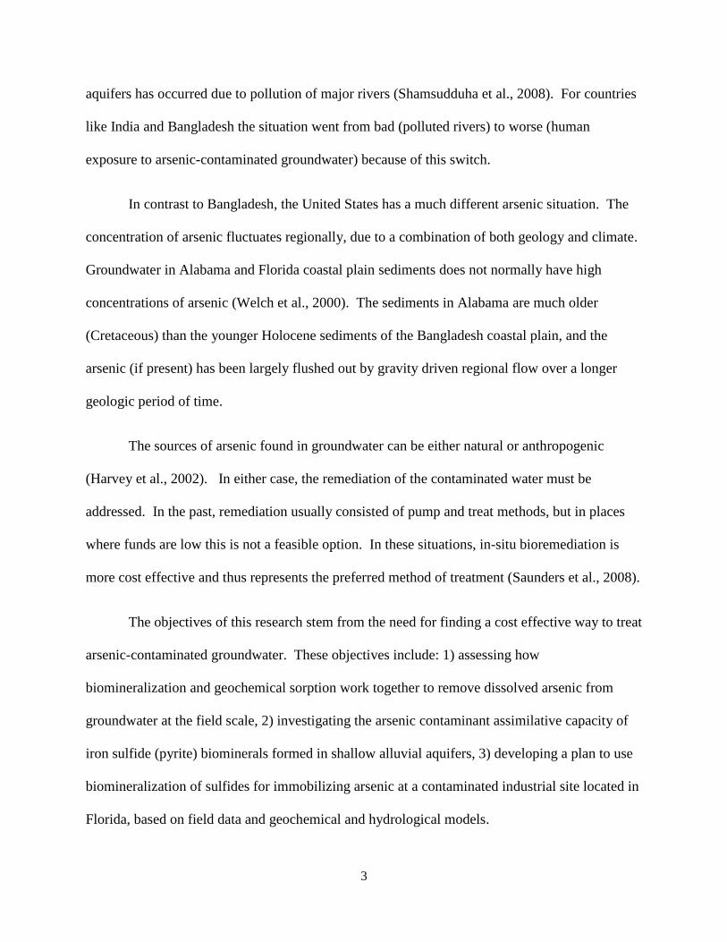
aquifers has occurred due to pollution of major rivers (Shamsudduha et al., 2008). For countries

like India and Bangladesh the situation went from bad (polluted rivers) to worse (human

exposure to arsenic-contaminated groundwater) because of this switch.

In contrast to Bangladesh, the United States has a much different arsenic situation. The

concentration of arsenic fluctuates regionally, due to a combination of both geology and climate.

Groundwater in Alabama and Florida coastal plain sediments does not normally have high

concentrations of arsenic (Welch et al., 2000). The sediments in Alabama are much older

(Cretaceous) than the younger Holocene sediments of the Bangladesh coastal plain, and the

arsenic (if present) has been largely flushed out by gravity driven regional flow over a longer

geologic period of time.

The sources of arsenic found in groundwater can be either natural or anthropogenic

(Harvey et al., 2002). In either case, the remediation of the contaminated water must be

addressed. In the past, remediation usually consisted of pump and treat methods, but in places

where funds are low this is not a feasible option. In these situations, in-situ bioremediation is

more cost effective and thus represents the preferred method of treatment (Saunders et al., 2008).

The objectives of this research stem from the need for finding a cost effective way to treat

arsenic-contaminated groundwater. These objectives include: 1) assessing how

biomineralization and geochemical sorption work together to remove dissolved arsenic from

groundwater at the field scale, 2) investigating the arsenic contaminant assimilative capacity of

iron sulfide (pyrite) biominerals formed in shallow alluvial aquifers, 3) developing a plan to use

biomineralization of sulfides for immobilizing arsenic at a contaminated industrial site located in

Florida, based on field data and geochemical and hydrological models.

4

Background

Geologic Setting

The first site of this study is located in Macon County, Alabama. At this site the coastal

plain aquifers and associated sediments rest in the Tuscaloosa Formation, which consists of non-

marine alluvial deposits that are considered undifferentiated (Penny et al., 2003). These

undifferentiated sediments consisting of gravel, sand, silt, and lignitized wood were derived from

the weathering and erosion of the Appalachians and were deposited in a Holocene floodplain

(Saunders et al., 2008). At this location (Figure 2), groundwater discharges locally into stream

banks of Uphapee Creek and Choctafaula Creek within Tuskegee National Forest (Saunders et

al., 1997). Age dating of organic clay at the base of the aquifer produced a date of 7000 years

before present (Markewich and Christopher, 1982). Arsenic and other trace metals (e.g., Co, Ni,

Cu, etc.) all occur in significant concentrations in biogenic pyrite found at this site (Saunders et

al., 1997). All of these hydrogeologic characteristics are similar to Holocene sediments of

southern Asia, permitting the comparison of the geochemical characteristics at the Macon

County site to those in Bangladesh.

The second location for this study is the Florida industrial site, where shallow

groundwater and sediments contain high levels of arsenic derived from pesticides. The Florida

industrial site lies within the Gulf Coastal Plain of the Florida panhandle (Figures 3 and 4). The

Florida panhandle falls within the East Gulf Coastal Plain section of the Coastal Plain

physiographic province. Within Bay County itself are four different physiographic subdivisions:

5

Figure 2. Location of the Macon County site (Alabama) where arsenic-rich

biogenic pyrite replaces wood fragments near the base of the coastal plain

alluvial aquifer. The occurrence of pyrite supports localized sulfate-reducing

conditions in which arsenic is sequestered in solids.

6

Figure 3. A map of northwest Florida showing the location of the Florida industrial site.

7

Figure 4. Site map of the Florida industrial site showing existing monitoring wells.

8

Sand Hills, Sinks and Lakes, Flat-Woods Forest, and Beach Dunes and Wave-cut Bluffs. The

Flat-Woods Forest subdivision takes up the largest portion of Bay County. Located within Bay

County the Florida industrial site rests in the Flat-Woods subdivision, and can be observed as

having a slightly rolling to flat topography covered in pine trees (except where it has been

cleared). Areas of the lowest elevations are likely to become flooded in times of heavy rainfall

(Schmidt and Clarke, 1980).

The deposition of thick sequences of marine sediments underneath Bay County is

controlled by the Apalachicola Embayment. The Apalachicola embayment is a regional basin

whose axis plunges to the southwest, producing increased sediment thickness towards the

coastline (Schmidt and Clarke, 1980). These sediments can be called marine terraces that

represent ancient sea floors receiving sedimentation. In addition to the Apalachicola

Embayment, other regional structures that may affect geology and sedimentation of the Gulf

Coastal Plain are the Chattahoochee Anticline and the Ocala Arch (Veach and Stephenson,

1911).

The oldest rocks found in outcrops exposed in the county are Early Miocene limestone

units. The youngest rocks found in the county are Pleistocene to recent aged undifferentiated

quartz sands, clayey sands, and gravels. These sands overlie the limestone units which can

extend to depths of 3000 feet, and below the limestone units, sandstones and shales extend to

granitic basement rock (Schmidt and Clarke, 1980).

There are four major hydrogeologic units that are recognized in the state of Florida:

surficial aquifer system, intermediate aquifer system (or the intermediate confining unit), the

Floridan aquifer system, and the sub-Floridan confining unit. The surficial aquifer system is

9

made up of undifferentiated terrace marine and fluvial deposits in the northern Florida panhandle

and normally consists of clayey sands and gravels near the coast (Schmidt and Clarke, 1980).

Specifically in Bay County, the surficial aquifer is mainly composed of quartz sand and

gravel with occasional clayey sand and sandy clay lenses (Schmidt and Clark, 1980).

Groundwater from the surficial aquifer discharges into local streams or springs, or it may migrate

into the deeper Floridan aquifer system where the two aquifer systems are hydraulically

interconnected. Underneath the surficial aquifer is the Jackson Bluff Formation, which is an

important intermediate confining unit that separates the surficial aquifer from the intermediate

aquifer. The Jackson Bluff Formation is characterized as sandy clay to clayey sand possessing

large portions of mollusk shells (Schmidt and Clark, 1980). Because of irregular deposition and

erosion, the Jackson Bluff Formation occurs intermittently in the southern portion of Bay County

and is more common in northern parts of the county.

10

Figure 5. Regional geologic structures of the Gulf Coastal Plain in Alabama, Florida,

and Georgia. This map shows the main structures controlling the deposition and

geologic properties of the Florida industrial site and surrounding areas (Modified

from Schmidt and Clark, 1980).

11

Figure 6. Geologic cross-section of Bay County showing the hydrogeologic units

from west to east across the county (Modified from Schmidt and Clark, 1980).

A A’

Florida Site

12

Figure 7. Generalized stratigraphic column for the Florida panhandle showing the main

stratigraphic and hydrostratigraphic units (Modified from Schmidt and Clark, 1980).

13

Florida Industrial Site History

Groundwater in the surficial aquifer beneath the Lynn Haven industrial site (Figure 3)

was contaminated via the use herbicides containing arsenic trioxide (a common by-product of the

copper smelting process). Extensive contamination assessment activities and analysis were

performed from 1989 to 1993 and confirmed that the contamination extended off-site to the north

and west with the highest arsenic concentration reaching about 4.5 ppm (Mintz and Miller,

1993).

In 1992, approximately 770 cubic yards of arsenic contaminated soil were removed and

disposed of in a nonhazardous waste landfill. In areas of close proximity to the soil excavation

arsenic concentrations in groundwater were reduced from 30 to 70 percent.

Remedial actions began at this site with the installation of a pump and treat system

utilizing a combination of iron co-precipitation, ceramic membrane filtration, and soil flushing

with selected reagents in 1994. These operations ended in 1999 due to the failure to further

lower arsenic concentrations below Florida Department of Environmental Protection (FDEP) and

EPA levels. At this time the site then began a monitor only program that was approved by FDEP.

The last excavation at this site occurred in 2008, at the suggestion of the FDEP.

Impacted soils along 11th street were removed based on data from previously collected soil

samples.

Arsenic Geochemistry

Arsenic that occurs in soil and groundwater can originate from both natural and

anthropogenic sources (USEPA, 1997). Natural sources of arsenic come from a large array of

14

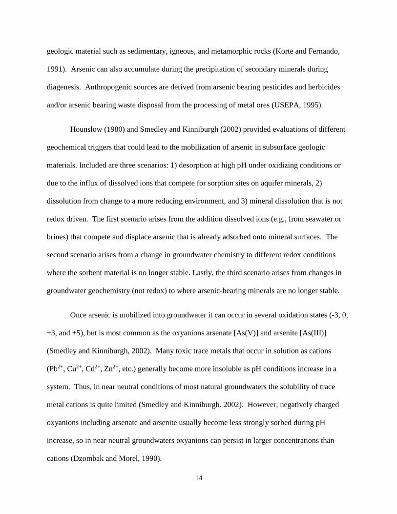
geologic material such as sedimentary, igneous, and metamorphic rocks (Korte and Fernando,

1991). Arsenic can also accumulate during the precipitation of secondary minerals during

diagenesis. Anthropogenic sources are derived from arsenic bearing pesticides and herbicides

and/or arsenic bearing waste disposal from the processing of metal ores (USEPA, 1995).

Hounslow (1980) and Smedley and Kinniburgh (2002) provided evaluations of different

geochemical triggers that could lead to the mobilization of arsenic in subsurface geologic

materials. Included are three scenarios: 1) desorption at high pH under oxidizing conditions or

due to the influx of dissolved ions that compete for sorption sites on aquifer minerals, 2)

dissolution from change to a more reducing environment, and 3) mineral dissolution that is not

redox driven. The first scenario arises from the addition dissolved ions (e.g., from seawater or

brines) that compete and displace arsenic that is already adsorbed onto mineral surfaces. The

second scenario arises from a change in groundwater chemistry to different redox conditions

where the sorbent material is no longer stable. Lastly, the third scenario arises from changes in

groundwater geochemistry (not redox) to where arsenic-bearing minerals are no longer stable.

Once arsenic is mobilized into groundwater it can occur in several oxidation states (-3, 0,

+3, and +5), but is most common as the oxyanions arsenate [As(V)] and arsenite [As(III)]

(Smedley and Kinniburgh, 2002). Many toxic trace metals that occur in solution as cations

(Pb2+, Cu2+, Cd2+, Zn2+, etc.) generally become more insoluble as pH conditions increase in a

system. Thus, in near neutral conditions of most natural groundwaters the solubility of trace

metal cations is quite limited (Smedley and Kinniburgh. 2002). However, negatively charged

oxyanions including arsenate and arsenite usually become less strongly sorbed during pH

increase, so in near neutral groundwaters oxyanions can persist in larger concentrations than

cations (Dzombak and Morel, 1990).

15

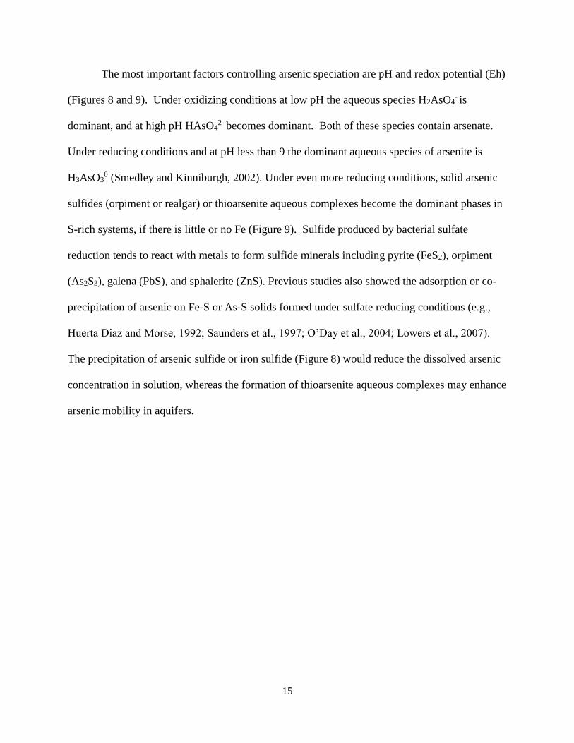
The most important factors controlling arsenic speciation are pH and redox potential (Eh)

(Figures 8 and 9). Under oxidizing conditions at low pH the aqueous species H2AsO4- is

dominant, and at high pH HAsO42- becomes dominant. Both of these species contain arsenate.

Under reducing conditions and at pH less than 9 the dominant aqueous species of arsenite is

H3AsO30 (Smedley and Kinniburgh, 2002). Under even more reducing conditions, solid arsenic

sulfides (orpiment or realgar) or thioarsenite aqueous complexes become the dominant phases in

S-rich systems, if there is little or no Fe (Figure 9). Sulfide produced by bacterial sulfate

reduction tends to react with metals to form sulfide minerals including pyrite (FeS2), orpiment

(As2S3), galena (PbS), and sphalerite (ZnS). Previous studies also showed the adsorption or co-

precipitation of arsenic on Fe-S or As-S solids formed under sulfate reducing conditions (e.g.,

Huerta Diaz and Morse, 1992; Saunders et al., 1997; O’Day et al., 2004; Lowers et al., 2007).

The precipitation of arsenic sulfide or iron sulfide (Figure 8) would reduce the dissolved arsenic

concentration in solution, whereas the formation of thioarsenite aqueous complexes may enhance

arsenic mobility in aquifers.

16

Figure 8. An Eh-pH diagram for aqueous arsenic species in the system

As-Fe-S-O2-H2O at 25oC and 1 bar pressure. The diagram was generated

with Geochemist’s Workbench.

17

Figure 9. An Eh-pH diagram showing the dominant solid phase arsenic

species in low Fe systems (As-S-H2O). Realgar and orpiment dominate

moderately reducing conditions and thioarsenate (As(SH)4-) aqueous

complexes dominate at even more reducing conditions. The diagram was

generated with Geochemist’s Workbench.

18

Previous Works

There are many published studies that characterize the speciation, mobilization, and

remediation of arsenic within aquifers. Examples include Lee and Saunders (2003), Saunders et

al. (2005 and 2008), Keimowitz et al. (2007), Shamsudduha et al. (2008), DeFlaun et al. (2009),

and Lutes et al. (2014).

Lee and Saunders (2003) and Saunders et al. (2005) presented studies in which a

geochemical reaction path model was constructed to trace the geochemical evolution (including

precipitation and adsorption reactions) of minerals and groundwater during an in-situ

bioremediation experiment. The in-situ bioremediation experiments were carried out at the

Sanders Lead car-battery recycling plant in Troy, Alabama. The geochemical models showed

the effects of redox potential (Eh) on mineral precipitation and pH controls on the sorption of

heavy metals. Modeling results showed that most metal ions remained in solution when pH was

below 3.5 and as pH increased over the reaction the sorption of metals on HFO’s became

significant. Dissolved Pb was strongly sorbed at low pH (less than 4), consistent with their field

observations. For As, increases in pH triggered increases in sorption for both arsenate and

arsenite (Figure 10A). However, arsenite dominates at lower pH than arsenate. The modeling

also showed that at low oxidation state As desorbs with increasing pH at approximately 5.8,

because of reactions with dissolved sulfide leading to the formation of arsenic sulfides (Figure

10B).

19

Saunders et al. (2005) studied the natural occurrence of arsenic in Holocene alluvial

aquifers and concluded arsenic derived from different geological sources such as mountain belts

or glacial deposits will be weathered, transported, and deposited in alluvial aquifers. This study

collected geochemical data from two sites in the United States where biogeochemical and

hydrogeologic conditions are comparable to arsenic contaminated sites in southern Asia. To

explain the mechanisms behind the natural contamination of arsenic, Saunders et al. (2005)

proposed that different geomicrobiologic, geochemical and hydrogeologic processes work

together to cause long distance transport and mobilization of arsenic in alluvial aquifers.

Tectonic uplift coupled with weathering and glaciation of bedrocks allowed for the release of

arsenic into streams where the As-bearing sediments were ultimately deposited and buried.

Eventually, anaerobic conditions will develop in these aquifers, and iron reducing bacteria will

Figure 10. A. Plot showing sorbed fractions of common metal ions versus an increase in pH.

B. Plot showing the concentration of sorbed As species versus a rise in pH.

(From Lee and Saunders, 2003).

A B

20

release the sorbed arsenic into solution. The steps in this geochemical cycling model explain and

help predict locations of potential arsenic contamination based on their geologic locations,

transport history, and local biogeochemical conditions.

Keimowitz et al. (2007) studied whether the method of enhanced sulfate reduction could

be a viable remediation strategy. Their samples were taken from a landfill in Maine that was

contaminated with arsenic. In both of their experiments, sediment, water, and acetate (carbon

source) were incubated. The first experiment analyzed small aqueous phase samples from large

vessel incubations, and the second experiment analyzed aqueous phase and sediment samples

Figure 11. An Eh and pH diagram showing the stability fields of Fe and As with

increasing pH as the microcosm experiment progressed with time (number of days in

bold). Sulfate reducing condition is established after about 39 days (from Keimowitz

et al., 2007).

21

from microcosm incubation. The results of this study showed that significant amounts of arsenic

were removed from solution by the forming of biogenic pyrite under highly reducing conditions

(with low negative Eh values) at the end of the both incubations (Figure 11). For the large vessel

incubation there was an approximate decrease in arsenic concentration of fifty percent. For the

microcosm experiment the arsenic concentration decreased by approximately 85 percent.

Saunders et al. (2008) presented new data from field bioremediation experiments and

geochemical modeling to illustrate the principal geochemical behavior of arsenic in anaerobic

groundwater. Two field bioremediation experiments were carried out, one in Bangladesh, where

carbon and MgSO4 were added to a shallow Holocene aquifer to stimulate sulfate reducing

bacteria. Another was in the United States, where groundwater was amended with sucrose and

methanol to stimulate sulfate reducing bacteria. These studies again showed that arsenic is

mobile and released from iron oxides under iron-reducing conditions and becomes immobile

under sulfate reducing conditions (Figure 12). Thus, if sulfate reduction can be engineered and

maintained, it is possible to reduce the arsenic concentration at the field scale.

The objectives of DeFlaun et al. (2009) were to examine the mineralogy of iron

hydroxides harboring arsenic and to measure the dissolution rate of the pyrite under aerobic

conditions. If arsenic sulfides formed in a lab setting would be stable on a decadal time scale

under changing redox conditions, then this technology may be feasible for a field remediation

strategy. The results of DeFlaun et al. (2009) showed successful sequestration of As under

anaerobic, sulfate reducing conditions, and that As precipitates were resistant to dissolution

under aerobic conditions (Figure 13).

22

Figure 12. Plot showing As and Fe concentration versus time for the Bangladesh

site. Arsenic concentrations were dramatically reduced one month after MgSO4

amendment (from Saunders et al., 2008).

Figure 13. The decrease in arsenic concentration with time from the DeFlaun et al.

(2009) pilot study.

23

Lutes et al. (2014) presented a study in which a field demonstration of in-situ

groundwater remediation technology was carried out. This technology was termed enhanced

anaerobic reductive precipitation (EARP) and enhanced reductive dechlorination (ERD). The

location of this study was the U.S. Department of Energy’s Savanah River Site (SRS). At this

location three key contaminants were targeted for remediation: uranium radionuclides,

technetium, and nitrate.

EARP involves the use of a food-grade carbohydrate substrate that acts as a food source

for microbiological processes. By injecting this food source into the subsurface, an aquifer that

is currently aerobic or mildly anoxic can be amended to a strongly anaerobic zone. This newly

amended anaerobic zone is suitable for the precipitation of metals and radionuclides in insoluble

forms or for the degradation of chlorinated solvents.

The goals of this field demonstration at the SRS were the attainment of continuous

sulfate-reducing biogeochemical conditions for a period of 18 months, achievement of treatment

goals for specific contaminants within two years in the main area of the reactive zone, and the

presence of precipitated uranium and technetium in insoluble sulfide forms following the

treatment.

By the end of the active treatment period redox zones were changed from aerobic to

methanogenic. At the target date of 18 months after injections the reactive zone of the SRS was

observed to be returning to original redox conditions, but still exhibited methane concentrations

suggesting that sulfate-reducing conditions were still ongoing.

The treatment goal for the key contaminants of concern at the SRS ended with mixed

results. The long-term trends for all contaminants fell sharply immediately after injection.

24

However, within a year of injection nitrate and strontium-90 were elevated above GWPS levels.

The remaining contaminants (U-233/234, U-238, and Tc-99) were still observed to be below

GWPS levels one year after injection.

Finally, the presence of precipitated insoluble forms of uranium and technetium can be

indicated by the continuing of long-term monitoring at the SRS site. For a successful test

precipitated uranium and technetium will not be re-dissolved at an unacceptable rate after

aerobic conditions are re-established. Most recent data collected 2.5 years after injections shows

that conditions have returned to background levels and the uranium radionuclides and technetium

concentrations have remained low, suggesting that sorbing mineral phases have formed and

remained stable in the aquifer.

25

Materials and Methods

Sample Collection and Water Quality Measurements

During January 21st through 24th 2015, Peter Starnes, Shahrzad Saffari, and Dr. Ming-

Kuo Lee of Auburn University, collected both sediment and water samples from the study site in

Lynn Haven, Florida. In addition to the collection of samples, in-situ measurements of water

quality parameters were also taken.

In order to collect representative sediment samples of the surficial aquifer at the Lynn

Haven site a peristaltic pump was used. Once the pump was placed into the well and lowered to

the bottom, sediments were collected into a clean beaker and then frozen in a test tube on dry ice

to preserve any bacteria or redox states of chemical species present in the well sediments.

To collect representative groundwater samples in the aquifer a peristaltic pump was used

to purge the wells. At least three well volumes of water were removed and all water quality

parameters readings became stable before sampling. This purging makes sure that all of the

stagnant groundwater residing inside the well casing is flushed out and fresh groundwater

percolates through the well screen. This procedure allows for the sample to accurately represent

the groundwater geochemistry of the aquifer being analyzed. After the well purging was

completed, water quality parameters including temperature, pH, dissolved oxygen, oxidation-

reduction potential, and electrical conductivity were measured in the field using YSI 556 hand-

held multiparameter probes. Measured ORP values are often normalized to a standard hydrogen

electrode (SHE), depending on the type of ORP electrode (e.g., Ag/AgCl) used. Since pH and

ORP electrodes are built together as a single probe for YSI 556, ORP is read relative to the

standard SHE, so no conversion of ORP measurements to Eh values is needed.

26

After a water sample was collected in a clean beaker, it was then filtered with a 45

micron filter and acidified with 5% nitric acid for preservation before trace metal and cation

analysis using inductively coupled plasma mass spectrometry (ICP-MS). A second sample was

filtered for anion analysis using ion chromatography (IC), as well as, DOC analysis. A third

sample for each well was filtered through arsenic speciation cartridges for an arsenic speciation

study. The sample was first filtered through a 45 micron filter and about 50 mL of the water

sample was passed through the cartridge using a syringe (with luer slip tip). The first 5 mL of

filtrate was discarded before collecting the filtered solution for analysis. The adsorbent in the

cartridges retains arsenate anions [As(V), H2AsO4-], but allows the uncharged arsenite complex

[As(III), or H3AsO3] to pass through. As(III) is then measured in the effluent filtered through the

cartridges and As(V) is calculated from the difference between total As and As(III). All water

samples were refrigerated for transport and preservation before chemical analysis.

Redox sensitive ions were measured in the field using HACH Spectrophotometers. A

HACH DR2700 was used to measure dissolved sulfide concentrations in the field via the

standard Methylene Blue Method (USEPA Method 8131). Ferrous iron concentrations were

measured by the 1.10 Phenanthroline Method (USEPA Method 8146) using a HACH DR820.

Alkalinity was also measured in the field using the standard titration method (USEPA Method

8203).

Monitoring Wells

Groundwater and sediment samples were collected from a total of 22 monitoring wells at

the Lynn Haven study site. All wells were drilled using hollow stem auger drilling procedures.

11 of the 22 wells were constructed of 2 inch diameter PVC casing, with a well screen of 0.01

27

inch slotted PVC, and are named “LH” wells. Each well had a fifteen-foot screened interval

used to monitor the surficial aquifer and to avoid breaching the Jackson Bluff confining layer.

Sand filter packs surround the screened interval and are placed at least one foot above the

interval. Over top of the sand filter pack, a bentonite seal of at least one foot was installed, and

all wells were grouted to the surface.

The remaining wells were installed as recovery and injection wells for the pump and treat

process that previously operated at this site, and are named “RA” wells. These wells were also

installed via hollow stem auger procedures. The RA wells were constructed with 6 inch PVC

pipe with five feet of screen below the water table.

Geochemical and Mineralogical Analyses

A total of 44 groundwater samples were shipped on ice to Actlabs Ltd. for major ion and

trace element analysis. 22 samples were tested for major anions using ion chromatography, and

the other 22 samples were tested for trace elements and cations using ICP-MS technology.

Biogenic pyrite samples (Figure 14) were also taken from the Macon County site, and

submitted to ACME Labs Inc. for aqua regia digestion followed by ICP-MS testing of the

remaining leachate. The aqua regia (3:1 volume ratios of HCl to HNO3) digestion procedure

(ISO standard 11466) is considered adequate for analyzing total acid leachable heavy metals in

sediments.

28

Fig

ure

14

. B

iogen

ic p

yri

te s

ample

fro

m M

acon C

ounty

, A

L s

ubm

itte

d t

o A

CM

E L

abs

Inc.

fo

r aq

ua

regia

dig

esti

on a

nd I

CP

-MS

tes

ting.

29

Dissolved organic carbon (DOC) analyses were performed to quantify the level of

organic matter contents in groundwater. 22 filtered groundwater samples from each well were

prepared for DOC analysis in the AU School of Forestry and Wildlife Sciences using a

Shimadzu TOC-V Combustion Analyzer.

X-ray fluorescence (XRF) and X-ray diffraction (XRD) technology were used to

determine the chemical compositions and mineralogical make-up of sediment samples collected

at the bottom of each well. Determining the mineralogy and chemistry of these sediments can

show the hydrogeology and geochemical conditions of the aquifer. The XRD and XRF analyses

were conducted using the Bruker D2 Phaser X-ray Diffraction spectrometer and the Bruker X-

ray Fluorescence Elemental Tracer IV-ED in the Department of Geosciences at Auburn

University. For XRD analysis, samples were run from 2 theta values of 27 degrees to 60 degrees

with a 0.004 degree step interval. The mineral composition of the samples was determined by a

peak search and match procedure using DIFFRAC.EVA software. XRD pattern also reveals

semi-quantitative make-up of a sample since the areas under the peak reflect the amount of each

phase present in the sample.

XRF technology analyzes the energy emission of characteristic fluorescent X-rays from a

sample that has been excited by bombardment with high-energy (i.e., short-wavelength) X-rays.

The XRF technology can quantify the elemental composition of a material because each element

has unique electronic orbitals of characteristic energy and the intensity of each characteristic

radiation is directly related to the amount of each element in the material. Major elements and

most trace elements (Ba, Cr, Co, Cu, Mo, Nb, Ni, Pb, Rb, Sr, U, Th, V, Y, Zn, Se, As, etc) of

sample, in the range of parts per million (ppm), were measured in the laboratory.

30

Hydrogeologic and Geochemical Modeling

To develop an effective remedial plan for the Lynn Haven industrial site, geochemical

and hydrogeologic modeling techniques were employed to characterize the site’s

hydrogeochemistry and groundwater flow regimes. The software Geochemist’s Workbench

(Bethke, 2008) was used to calculate speciation and geochemical reactions associated with

sulfate reduction based on the current field hydrochemical environment. Field parameters

measured (temperature, pH, Eh, etc.) and the concentrations of major ions and arsenic were

uploaded in a spreadsheet into Geochemist’s Workbench. Activity diagrams and hydrochemical

facies analysis were used to graphically characterize the geochemical conditions of Lynn Haven

surficial aquifer. Eh-pH diagrams are particularly useful in showing stable fields of various solid

and aqueous phases under different redox and geochemical conditions. Piper diagrams are used

to show the characteristic hydrochemical facies of groundwater in the surficial aquifer. In

addition, a reaction path model was created in Geochemist’s Workbench to predict what might

happen minerogically and chemically as a result of sulfate reduction within the surficial aquifer.

Three dimensional numerical modeling of groundwater flow and contaminant transport at

the Lynn Haven site was performed using the U.S. Geological Survey model MODFLOW

(McDonald and Harbaugh, 1988). The governing equation for 3D groundwater transient

simulation is:

𝑆𝑠𝜕ℎ

𝜕𝑡− 𝑅∗ =

𝜕

𝜕𝑥(𝐾𝑥

𝜕ℎ

𝜕𝑥) +

𝜕

𝜕𝑦(𝐾𝑦

𝜕ℎ

𝜕𝑦) +

𝜕

𝜕𝑧(𝐾𝑧

𝜕ℎ

𝜕𝑧)

where h is hydraulic head, Ss is specific storage, and Kx, Ky, and Kz are hydraulic conductivity in

x, y, and z directions. R* represents a source term derived from water pumping or injection. The

31

solute transport equation involved advection, dispersion, and adsorption processes in one

dimension is given by:

𝜕𝐶

𝜕𝑡= −𝑣

𝜕𝐶

𝜕𝑥+ 𝐷

𝜕2𝐶

𝜕𝑥2−𝜌𝑏𝜑

𝜕(𝐾𝑑𝐶)

𝜕𝑡

where C is the concentration of a given contaminant (mol cm-3), v is groundwater flow velocity

(cm sec-1), t is time (sec), and D is hydrodynamic dispersion (cm2 sec-1), which accounts for

molecular diffusion of solutes as well as mechanical dispersion. The model calculates the

coefficients of hydrodynamic dispersion D from the following equation:

D = D* + vx

where D* is the diffusion constant (cm2 sec-1) and is the dispersivity (cm) in the x direction.

Graphic interface modeling was carried out with the programs Visual Modflow Classic

and Visual Modflow Flex. These two programs are industry standards in characterizing the

groundwater hydrogeology of an aquifer and are distributed by Schlumberger Water Services.

The input parameters required for modeling a system were: conductivities, porosities, storage

capacity, initial heads, concentration observations, observed head values, contaminant

concentrations, hydraulic gradient, recharge, precipitation, and groundwater boundaries. All of

these variables were gathered through the January 2015 sampling event and in previous studies

(Mintz and Miller, 1993). By using measured field hydrogeologic parameters and proper

boundary and initial conditions numerical models of groundwater flow were generated.

Sensitivity analysis was also conducted to examine the effects of adsorption on arsenic transport.

32

Results and Discussion

Groundwater Geochemistry

Tables 1 and 2 show the complete results of the geochemical analyses of this study.

Table 1 lists the field parameters that were measured during the January 2015 sampling event.

The water temperatures encountered in the wells ranged from 14.5°C to 22.4°C. The mean

groundwater temperature was 18.46°C with a standard deviation of 1.74°C.

The pH values for groundwater in the Lynn Haven surficial aquifer were observed to be

near-neutral to slightly acidic, as expected for a coastal plain surficial aquifer. The observed pH

ranges from 4.46 in LH-25 and 6.82 in RA-11. The mean pH was calculated to be 5.72 with a

standard deviation of 0.65.

Oxidation-reduction potential (ORP) was also measured in the field during the January

2015 sampling event. The highest ORP recorded occurred in well LH-25 at 130.4 mV, and the

lowest ORP value was recorded in well RA-4 at -77 mV. The mean value for field ORP was

46.72 mV and the standard deviation of ORP was 40.03 mV. ORP is determined by measuring

the potential of a chemically-inert electrode which is immersed in the solution. The sensing

electrode potential is then read in reference to the electrode of the pH probe and presented in

mV. Because the values are already referenced to the standard hydrogen electrode (SHE) in the

pH probe they do not need to be referenced again to be used as Eh values. This will be discussed

in more detail in the results of the geochemical modeling section.

33

Well I

DT

em

p (

°C)

pH

OR

P (

mV

)C

onduct

ivit

y (μ

s/cm

)S

2- (

mg/

L)

Fe

2+

(mg/

L)

Alk

alinit

y (

mg/

L)

DO

(m

g/L

)

LH

-218

5.2

942

164

0.0

10.4

240

0.4

2

LH

-417.7

5.8

678.4

149

0.1

40.6

780

0.6

LH

-516.4

56.4

256

227

0.0

10.1

779

1.5

9

LH

-716.9

5.7

33.7

200

0.0

61.4

878

0.2

5

LH

-12

19.6

5.5

36

233

0.3

00.2

520

0.2

4

LH

-15

19.4

54.7

44.1

80

0.1

90.7

84

0.1

8

LH

-16

18.6

55

51.2

109

0.4

30.8

18

0.1

9

LH

-19

20.2

4.5

890

62

0.1

60.2

58

0.9

5

LH

-25

22.4

4.4

6130.4

94

0.3

40.0

94

0.1

LH

-26

20.8

5.1

61

110

0.0

90.6

430

0.1

6

LH

-27

17.2

5.7

6105

124

0.0

40.3

218

0.9

5

RA

-119.4

6.1

528

77

0.0

21.6

335

0.1

5

RA

-218.5

5.8

363

206

0.0

12.7

446

0.1

4

RA

-318.1

6.2

7-1

2125

0.0

02.4

460

0.7

6

RA

-418.2

6.1

-77

167

0.0

61.2

568

0.0

9

RA

-520.5

5.7

241

233

0.1

81.5

645

0.0

9

RA

-917.1

6.1

235

130

0.0

70.0

331

1.5

3

RA

-10

16.7

6.7

146

278

0.0

10.1

195

0.5

5

RA

-11

14.5

6.8

249

166

0.0

30.1

251

1.5

5

RA

-12

18.4

5.7

436

299

0.0

40.9

128

1.4

9

RA

-13

17.6

5.7

339

102

0.0

10.1

325

0.8

5

RA

-14

19.7

6.3

852

133

0.0

30.0

848

0.8

1

Mean

18.4

65.7

246.7

2157.6

40.1

00.7

740.9

50.6

2

Sta

n. D

ev.

1.7

40.6

540.0

366.2

10.1

20.7

826.8

10.5

3

Tab

le 1

. F

ield

par

amet

er r

esult

s fr

om

the

Januar

y 2

015 s

ampli

ng e

ven

t. E

lect

rica

l co

ndu

ctiv

ity i

s

mea

sure

d i

n μ

S/c

m. U

nit

s fo

r su

lfid

e (S

2- )

and f

erro

us

iron (

Fe2

+)

are

mg/L

. F

ield

OR

P v

alues

wer

e

mea

sure

d i

n r

efer

ence

to t

he

elec

trod

e of

the

pH

met

er o

f Y

SI-

556, th

us

can

be

use

d a

s E

h v

alues

wit

hout

bei

ng r

efer

ence

d.

34

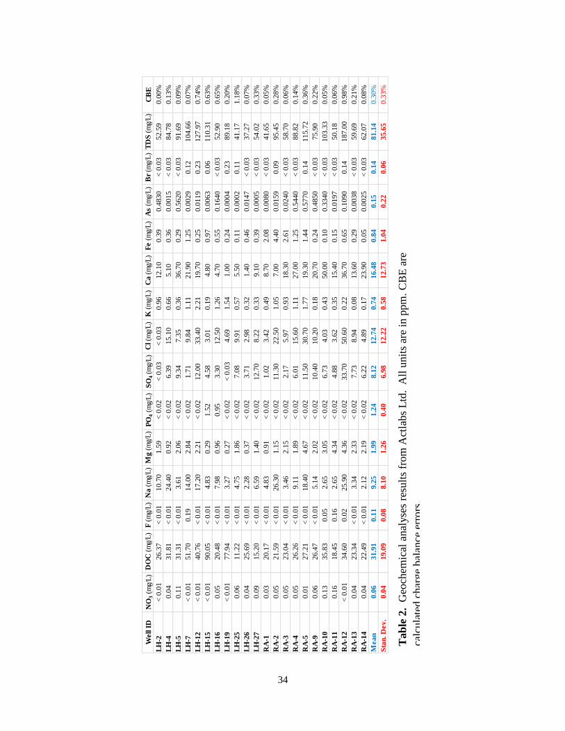
Tab

le 2

. G

eoch

emic

al a

nal

yse

s re

sult

s fr

om

Act

labs

Ltd

. A

ll u

nit

s ar

e in

ppm

. C

BE

are

calc

ula

ted c

har

ge

bal

ance

err

ors

.

Well I

DN

O3 (

mg/

L)

DO

C (

mg/

L)

F (

mg/

L)

Na (

mg/

L)

Mg (

mg/

L)

PO

4 (

mg/

L)

SO

4 (

mg/

L)

Cl (m

g/L

)K

(m

g/L

)C

a (

mg/

L)

Fe (

mg/

L)

As

(mg/

L)

Br

(mg/

L)

TD

S (

mg/

L)

CB

E

LH

-2<

0.0

126.3

7<

0.0

110.7

01.5

9<

0.0

2<

0.0

3<

0.0

30.9

612.1

00.3

90.4

830

< 0

.03

52.5

90.0

0%

LH

-40.0

431.8

1<

0.0

124.4

00.9

2<

0.0

26.3

915.1

00.6

65.1

00.3

60.0

015

< 0

.03

84.7

80.1

3%

LH

-50.1

131.3

1<

0.0

13.6

12.0

6<

0.0

29.3

47.3

50.3

636.7

00.2

90.5

620

< 0

.03

91.6

90.0

9%

LH

-7<

0.0

151.7

00.1

914.0

02.8

4<

0.0

21.7

19.8

41.1

121.9

01.2

50.0

029

0.1

2104.6

60.0

7%

LH

-12

< 0

.01

40.7

6<

0.0

117.2

02.2

1<

0.0

212.0

033.4

02.2

119.7

00.2

50.0

119

0.2

3127.9

70.7

4%

LH

-15

< 0

.01

90.0

5<

0.0

14.8

30.2

91.5

24.5

83.0

10.1

94.8

00.9

70.0

063

0.0

6110.3

10.6

3%

LH

-16

0.0

520.4

8<

0.0

17.9

80.9

60.9

53.3

012.5

01.2

64.7

00.5

50.1

640

< 0

.03

52.9

00.6

5%

LH

-19

< 0

.01

77.9

4<

0.0

13.2

70.2

7<

0.0

2<

0.0

34.6

91.5

41.0

00.2

40.0

004

0.2

389.1

80.2

0%

LH

-25

0.0

611.2

2<

0.0

14.7

51.8

6<

0.0

27.0

89.9

10.5

75.5

00.1

10.0

002

0.1

141.1

71.1

8%

LH

-26

0.0

425.6

9<

0.0

12.2

80.3

7<

0.0

23.7

12.9

80.3

21.4

00.4

60.0

147

< 0

.03

37.2

70.0

7%

LH

-27

0.0

915.2

0<

0.0

16.5

91.4

0<

0.0

212.7

08.2

20.3

39.1

00.3

90.0

005

< 0

.03

54.0

20.3

3%

RA

-10.0

320.1

7<

0.0

14.8

30.9

1<

0.0

21.0

23.4

20.4

98.7

02.0

80.0

080

< 0

.03

41.6

50.0

5%

RA

-20.0

521.5

9<

0.0

126.3

01.1

5<

0.0

211.3

022.5

01.0

57.0

04.4

00.0

159

0.0

995.4

50.2

8%

RA

-30.0

523.0

4<

0.0

13.4

62.1

5<

0.0

22.1

75.9

70.9

318.3

02.6

10.0

240

< 0

.03

58.7

00.0

6%

RA

-40.0

526.2

6<

0.0

19.1

11.8

9<

0.0

26.0

115.6

01.1

127.0

01.2

50.5

440

< 0

.03

88.8

20.1

4%

RA

-50.0

127.2

1<

0.0

118.4

04.6

7<

0.0

211.5

030.7

01.7

719.3

01.4

40.5

770

0.1

4115.7

20.3

6%

RA

-90.0

626.4

7<

0.0

15.1

42.0

2<

0.0

210.4

010.2

00.1

820.7

00.2

40.4

850

< 0

.03

75.9

00.2

2%

RA

-10

0.1

335.8

30.0

52.6

53.0

5<

0.0

26.7

34.0

30.4

350.0

00.1

00.3

340

< 0

.03

103.3

30.0

5%

RA

-11

0.1

618.4

50.1

62.6

54.3

4<

0.0

24.8

83.6

20.3

515.4

00.1

50.0

197

< 0

.03

50.1

80.0

6%

RA

-12

< 0

.01

34.6

00.0

225.9

04.3

6<

0.0

233.7

050.6

00.2

236.7

00.6

50.1

090

0.1

4187.0

00.9

8%

RA

-13

0.0

423.3

4<

0.0

13.3

42.3

3<

0.0

27.7

38.9

40.0

813.6

00.2

90.0

038

< 0

.03

59.6

90.2

1%

RA

-14

0.0

422.4

9<

0.0

12.1

22.1

9<

0.0

26.2

24.8

90.1

723.9

00.0

50.0

025

< 0

.03

62.0

70.0

8%

Mean

0.0

631.9

10.1

19.2

51.9

91.2

48.1

212.7

40.7

416.4

80.8

40.1

50.1

481.1

40.3

0%

Sta

n. D

ev.

0.0

419.0

90.0

88.1

01.2

60.4

06.9

812.2

20.5

812.7

31.0

40.2

20.0

635.6

50.3

3%

35

Conductivity values ranged from 62 μS/cm in well LH-19 to 299 μS/cm in well RA-12.

The mean conductivity for the surficial aquifer was 157.64 μS/cm and the standard deviation was

66.21 μS/cm. Conductivity values correspond to the total dissolved solids (TDS) of the

groundwater. The more dissolved solids are present in the water the higher the electrical

conductance of a sample, especially if there are dissolved metals and metalloids present.

Alkalinity can be defined as the net concentration of strong base in excess of a strong

acid with a pure CO2 system as a point of reference (Morel, 1983). In natural groundwater, the

generation of a net positive charge through the dissolution of carbonate minerals is usually

greater than the contribution of negative charges from the ionization of strong acids (Domenico

and Schwartz, 1990). Thus, as a general rule of thumb, natural groundwaters typically will

display a positive alkalinity, unless there is some point of strong acidic contamination. The

results of our field measurements of alkalinity (as HCO3-) yielded an average mode of 40.95

mg/L with a standard deviation of 26.81 mg/L. These results can be expected for the Lynn Haven

aquifer, since there are few carbonate minerals in the surficial aquifer and recharge is mainly of a

meteoric origin. Groundwater in the surficial aquifer may still acquire alkalinity via mixing with

deeper groundwater associated with the Bruce Creek Limestone.

Dissolved oxygen (DO) was also measured in the field with the YSI-556. The highest DO

measurement was taken at well LH-5 at 1.59 mg/L. The lowest DO was observed at wells RA-4

and RA-5 at 0.09 mg/L. DO values are generally low as compared to those in shallow aquifers

or surface water under oxidizing conditions. Dissolved oxygen concentration will reduce to low

levels due to breakdown or degradation of organic matter in the aquifer. The relatively low DO

values are consistent with ORP values that indicate a moderately reducing environment.

36

Table 2 shows the results of geochemical analyses including measured major cation

concentration, major anion concentration, trace element (As and Fe) composition, dissolved

organic carbon (DOC), and TDS calculated from these concentrations. NO3 (nitrate)

concentrations ranged from below the detection limit (0.01 ppm) in several wells to 0.16 ppm in

well RA-11. The average NO3 concentration was calculated to be 0.06 ppm with a standard

deviation of 0.04 ppm. The relatively low values for this aquifer are expected, since there are no

surficial sources of excess nitrate in the area (fertilizers).

Naturally occurring dissolved organic carbon (DOC) in groundwater is produced by

biological and biochemical decay of organic matter in the aquifer. Results indicate the lowest

DOC value of 11.22 ppm in well LH-25 and the highest value of 90.05 ppm in LH-15. The

mean DOC value was calculated to be 31.91 ppm with a standard deviation of 19.09 ppm. The

relatively low DOC values indicate that the aquifer needs to be amended with organic carbon and

nutrients to boost the activity of sulfate-reducing bacteria during biostimulation.

Fluorine, which usually occurs as fluoride (F-) in natural groundwaters, was measured. In

all but 4 wells, LH-7, RA-10, RA-11, and RA-12, fluoride concentrations were below detection

limits. The main sources for fluoride in groundwater are the minerals fluorite and apatite. None

of these minerals are present in aquifer materials, so expected results for fluoride should be low.

Sodium (Na) is another major constituent of groundwater and typically occurs as the ion

Na+. Sodium concentrations ranged from 26.30 ppm in RA-2 and 2.12 ppm in RA-14. The

mean sodium concentration was calculated to be 9.25 ppm with a standard deviation of 8.10

ppm.

37

Magnesium (Mg) occurs in groundwater as the ion Mg2+ and is considered another major

constituent of groundwater. From the water samples collected during the January 2015 sampling

event Mg2+ concentrations ranged from 4.67 ppm in well RA-5 and 0.29 ppm in well LH-15.

The mean Mg2+ concentration was 1.99 ppm with a standard deviation of 1.26 ppm.

Phosphate (PO4) concentrations in the Lynn Haven Surficial Aquifer occurred at very low

concentrations. In all but 2 wells (LH-15 and LH-16), phosphate levels were below the detection

limit (0.01 ppm). The relatively low values for this aquifer are expected, since there are no

surficial sources of excess nitrate in the area (fertilizers).

Sulfide (S2-) concentrations measured range from 0.01 ppm in several wells to 0.43 ppm

in well LH-16. The calculated mean for sulfur concentrations was 0.10 ppm and the standard

deviation was 0.12 ppm. High sulfide concentrations in certain locations may be resulting from

bacterial sulfate reduction, as indicated by its typical rotten egg smell.

Sulfate (SO42-) is a major ion found in surface water, seawater, and groundwater. At the

Lynn Haven site, SO42- concentrations ranged from below detection (<0.03 ppm) in well LH-2

and LH-19 to 33.7 ppm in well RA-12. The mean sulfate concentration was 8.12 ppm and the

standard deviation was 6.98 ppm.

Chlorine is commonly found in water as the ion chloride (Cl-). The chloride

concentration of the Lynn Haven Surficial Aquifer ranged from below detection (<0.03 ppm) in

well LH-2 to 50.60 ppm in well RA-12. The mean concentration was 12.74 ppm with a standard

deviation of 12.22 ppm.

Potassium found in water exists as the ion K+. Results from the January 2015

groundwater sampling showed that potassium concentrations ranged from 0.08 ppm in well RA-

38

13 and 2.21 ppm in well LH-12. The mean concentration of potassium in groundwater samples

was 0.74 ppm with a standard deviation of 0.58 ppm.

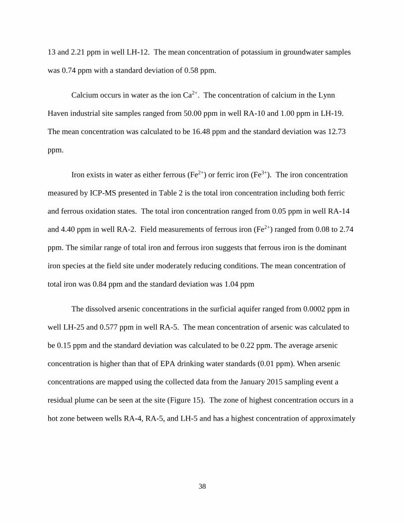
Calcium occurs in water as the ion Ca2+. The concentration of calcium in the Lynn

Haven industrial site samples ranged from 50.00 ppm in well RA-10 and 1.00 ppm in LH-19.

The mean concentration was calculated to be 16.48 ppm and the standard deviation was 12.73

ppm.

Iron exists in water as either ferrous (Fe2+) or ferric iron (Fe3+). The iron concentration

measured by ICP-MS presented in Table 2 is the total iron concentration including both ferric

and ferrous oxidation states. The total iron concentration ranged from 0.05 ppm in well RA-14

and 4.40 ppm in well RA-2. Field measurements of ferrous iron (Fe2+) ranged from 0.08 to 2.74

ppm. The similar range of total iron and ferrous iron suggests that ferrous iron is the dominant

iron species at the field site under moderately reducing conditions. The mean concentration of

total iron was 0.84 ppm and the standard deviation was 1.04 ppm

The dissolved arsenic concentrations in the surficial aquifer ranged from 0.0002 ppm in

well LH-25 and 0.577 ppm in well RA-5. The mean concentration of arsenic was calculated to

be 0.15 ppm and the standard deviation was calculated to be 0.22 ppm. The average arsenic

concentration is higher than that of EPA drinking water standards (0.01 ppm). When arsenic

concentrations are mapped using the collected data from the January 2015 sampling event a

residual plume can be seen at the site (Figure 15). The zone of highest concentration occurs in a

hot zone between wells RA-4, RA-5, and LH-5 and has a highest concentration of approximately

39

Fig

ure

15

. A

conto

ur

map

of

arse

nic

dis

trib

uti

on a

t th

e L

ynn H

aven

indust

rial

sit

e.

12

0 m

9

0

60

3

0

40

0.550 ppm. Historically, the highest arsenic concentration reached about 4.50 ppm before pump-

and-treat remediation (Mintz and Miller, 1993). Results of ICP-MS analysis show that arsenic

concentrations of biogenic pyrite at the Macon County site reach approximately 3670 ppm As.

Another major constituent of groundwater is the bromide ion (Br-). The concentration of

bromide in the Lynn Haven wells ranged from below detection (<0.03 ppm) in several wells and

0.23 ppm in well LH-12 and LH-19. The mean bromide concentration was 0.14 ppm and the

standard deviation was 0.06 ppm.

The last parameter measured in the Table 2 is that of TDS (total dissolved solids). This

value correlates well with conductivity in Table 1. The well with the highest TDS should also

have the highest conductivity. TDS in the surficial aquifer groundwater samples ranged from

37.35 ppm in well LH-26 and 187.04 ppm in well RA-12. The mean TDS was calculated to be

81.24 ppm with a standard deviation of 35.65 ppm.

Groundwater Mixing and Water-Rock Interaction

Plots of major ion (Na+, Ca2+, Mg2+, K+, SO42-) concentrations against chloride

concentrations (Figures 16 to 20) relative to the conservative seawater dilution trend, reveal that

different water-rock processes (e.g., precipitation, dissolution, and ion exchange) occur to

varying extent as well as potential mixing of deep carbonate groundwater (Drever, 1997).

Figure 16 shows the sodium concentration versus the chloride concentration with the

conservative mixing line. Most data taken from the well samples falls on or close to the mixing

line, suggesting conservative mixing of seawater with freshwater in the surficial aquifer. Points

plotted above or below the conservative mixing line may be explained by Na exchange or

fixation on clays. Clay-rich Jackson Bluff Formation is present underneath the surficial aquifer.

41

0.00

5.00

10.00

15.00

20.00

25.00

30.00

0.00 10.00 20.00 30.00 40.00 50.00 60.00

Na (

pp

m)

Cl (ppm)

Figure 16. Sodium concentration versus chloride concentration of the surficial aquifer.

The bold line represents the conservative mixing of seawater with freshwater.

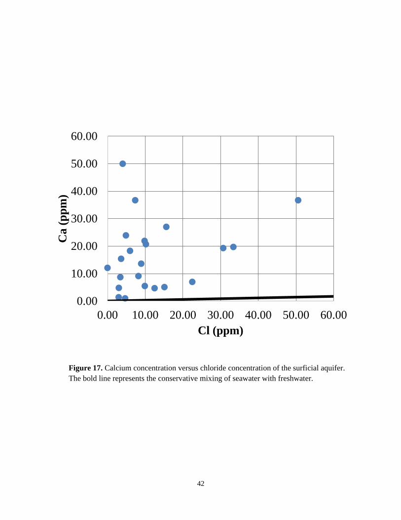
42

0.00

10.00

20.00

30.00

40.00

50.00

60.00

0.00 10.00 20.00 30.00 40.00 50.00 60.00

Ca (

pp

m)

Cl (ppm)

Figure 17. Calcium concentration versus chloride concentration of the surficial aquifer.

The bold line represents the conservative mixing of seawater with freshwater.

43

0.00

1.00

2.00

3.00

4.00

5.00

6.00

7.00

0.00 20.00 40.00 60.00

Mg (

pp

m)

Cl (ppm)

Figure 18. Magnesium concentration versus chloride concentration of the surficial

aquifer. The bold line represents the conservative mixing of seawater with freshwater.

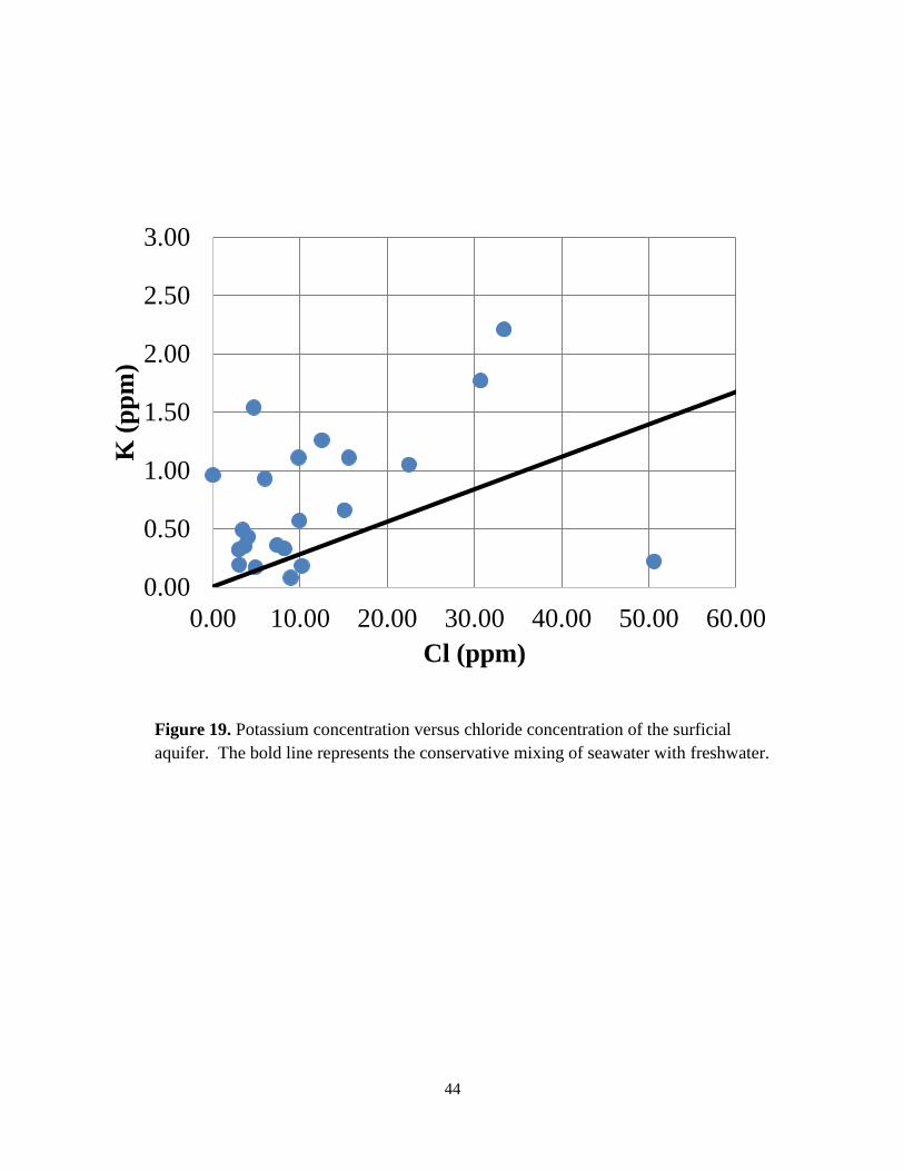
44

0.00

0.50

1.00

1.50

2.00

2.50

3.00

0.00 10.00 20.00 30.00 40.00 50.00 60.00

K (

pp

m)

Cl (ppm)

Figure 19. Potassium concentration versus chloride concentration of the surficial

aquifer. The bold line represents the conservative mixing of seawater with freshwater.

45

Fig

ure

20

. S

ulf

ate

conce

ntr

atio

n v

ersu

s th

e ch

lori

de

conce

ntr

atio

n o

f th

e su

rfic

ial

aquif

er. T

he

bold

lin

e

repre

sents

the

conse

rvat

ive

mix

ing o

f se

awat

er w

ith

fre

shw

ater

.

46

For example, cation exchange reaction of the following equation would produce a NaHCO3 type

water with high Na contents (Appelo, 1994: Penny et al., 2003):

CaCO3 + Na2-clay + H+ Ca-clay + 2 Na+ + HCO3-

Furthermore, ion exchange between Na and a divalent cation such as Ca may be expressed as the

following reaction (Drever, 1997):

Ca-clay + Na+ 2 Na-Clay + Ca2+

When the aquifer is invaded by saline seawater, the resulting salinization may cause monovalent

ions (Na) in groundwater to replace divalent ions (Ca) from the clay. Groundwater affected by

saltwater intrusion and subsequent ion exchange thus tends to be depleted in Na+ with lower

Na/Cl molar ratios (Drever, 1997). At the study site, groundwater with higher salinity tends to

be slightly depleted in Na+ (Figure 16).

Figures 17 and 18 plot calcium and magnesium concentration versus chloride

concentration of the sampled wells along with the conservative mixing line for seawater and

freshwater. The results indicate that there are strong enrichments of both calcium and

magnesium in the surficial aquifer. This may be attributed to carbonate stratigraphic units

(Bruce Creek Limestone) below the surficial aquifer where the Jackson Bluff confining bed is

not present (Schmidt and Clark, 1980). The Jackson Bluff confining unit is locally absent in the

eastern part of Bay County (Figure 5), leading to possible sites of calcium enrichment. The

enrichments of Ca and Mg may be also attributed to ion exchange processes (see equation above)

when the aquifer is diluted by freshwater (Drever, 1997). The dolomitization process,

represented by the following reaction:

47

2CaCO3 + Mg2+ MgCa(CO3)2 + Ca2+

would release Ca but consume Mg in the solution. Thus, dolomitization or de-dolomitization is

not likely to cause the simultaneous enrichments of Ca and Mg in solution (Drever, 1997).

Figure 19 show the concentrations of potassium versus chloride concentration. The result

also suggests a slight enrichment of potassium. External sources for potassium may be from

seawater or saline formation water from the Jackson Bluff confining unit since it is in direct

contact with the surficial aquifer (Schmidt and Clark, 1980).

Figure 20 shows the concentrations of sulfate versus chloride relatively to conservative

mixing line. Most of the data plots slightly above or along the mixing line. This suggests a

slight enrichment of sulfate relative to seawater dilution trend. The result implies that local

sulfate reduction has not removed all available sulfate in the aquifer.

Iron and Arsenic Speciation

As stated earlier, the dominant iron species at the Lynn Haven industrial site is ferrous

iron (Fe2+). Field measurement of ferrous iron was plotted against the lab measurements of total

iron (Figure 21). The plot shows an approximately 1:1 ratio of ferrous and total iron

concentration, suggesting that the ferrous iron is the dominant species. However, there were

some instances where the ferrous measurements exceeded the total iron measurements. This

may be caused by different instrumental methods used in field and laboratory measurements.

For arsenic speciation, geochemical modeling results conducted in this study (Figure 22) indicate

that arsenite [As(III)] should be the dominated species in the groundwater at the site under

moderately reducing conditions. Laboratory measurements of various arsenic species are

48

0.00

0.50

1.00

1.50

2.00

2.50

3.00

0.00 1.00 2.00 3.00 4.00 5.00

Fe

2+

Total Fe (ppm)Figure 21. Plot of Ferrous iron concentration versus the total iron concentration of the

surficial aquifer. The bold line represents a 1:1 ratio of the two concentrations.

49

Figure 22. An Eh-pH diagram for the predicted dominant As phases at the Lynn

Haven site (blue fields are aqueous phases and tan fields are solid phases). Plotted on

the diagram are the redox conditions for each water sample collected.

50

underway using new ICP-MS facilities at Auburn. The results will be addressed in another

study.

XRF and XRD Analysis Results

Selected sediment samples also underwent XRD and XRF analyses (Figures 23 to 30).

XRF analyses were used to identify the chemical composition of sediment slurry deposited

inside the well casing before remediation. XRF analyses of representative samples consistently

resulted in major peaks for Fe, S, and As (Figures 23-27). The spectra were created using the

voltage and current settings of 40 KeV and 18 µA (filter #1) without vacuum. This suggests that

minor precipitation of pyrite is already taking place in the zones of sulfate reduction. Results of

Larger peaks correspond to larger concentrations, but XRF results should only be taken

qualitatively. Quantitative ICP-MS analysis shows that arsenic concentrations of biogenic

pyrite at the Macon County site reach approximately 3670 ppm As.

Dark sediment slurry samples collected from well RA-5 tested positive for the presence

of elements Fe, S, and As. The presence of these elements supports the idea the arsenic bearing

pyrite is already be formed locally under reducing conditions. Wells LH-12, LH-19, and LH-26

not only showed positive results for Fe, S, and As, but also showed elevated concentrations of

other trace metals that will not be addressed in this study. Interestingly, well LH-25 samples

showed a stronger signature for Zn than Fe (Figure 26); this may suggest that sphalerite may also

be precipitating if enough zinc is present.

XRD analyses were carried out to show what minerals are present in a given sample.

This was done to compliment XRF results and compare dominant minerals to dominant elements

to make sure that there is some degree of accordance.

51

Fig

ure

23

. X

RF

spec

tra

of

elem

ents

pre

sent

in t

he

sedim

ent

sam

ple

of

wel

l R

A-5

. T

he

colo

red l

ines

rep

rese

nt

the

pea

k l

oca

tions

for

the

label

ed e

lem

ents

.

52

Fig

ure

24

. X

RF

spec

tra

of

elem

ents

pre

sent

in t

he

sedim

ent

sam

ple

of

wel

l L

H-1

2. T

he

colo

red l

ines

rep

rese

nt

the

pea

k l

oca

tions

for

the

label

ed e

lem

ents

.

53

Fig

ure

25

. X

RF

spec

tra

of

elem

ents

pre

sent

in t

he

sedim

ent

sam

ple

of

wel

l L

H-1

9. T

he

colo

red l

ines

rep

rese

nt

the

pea

k l

oca

tions

for

the

label

ed e

lem

ents

.

54

Zn

Ru

F

e R

u

Fig

ure

26

. X

RF

spec

tra

of

elem

ents

pre

sent

in t

he

sedim

ent

sam

ple

of

wel

l L

H-2

5. T

he

colo

red l

ines

repre

sent

the

pea

k l

oca

tions

for

the

label

ed e

lem

ents

.

55

Fig

ure

27

. X

RF

spec

tra

of

elem

ents

pre

sent

is t

he

sedim

ent

sam

ple

of

wel

l L

H-2

6. T

he

colo

red l

ines

repre

sent

the

pea

k l

oca

tions

for

the

label

ed e

lem

ents

.

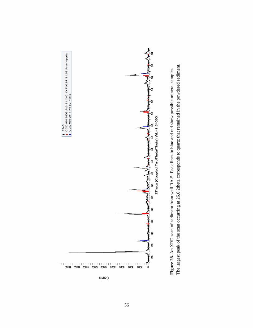
56

Fig

ure

28

. A

n X

RD

sca

n o

f se

dim

ent

from

wel

l R

A-5

; P

eak l

ines

in b

lue

and r

ed s

how

po

ssib

le m

iner

al s

amp

les.

Th

e la

rges

t pea

k o

f th

e sc

an o

ccurr

ing a

t 26.6

2th

eta

corr

esponds

to q

uar

tz t

hat

rem

ained

in

th

e p

ow

der

ed s

edim

ent.

57

Fig

ure

29

. A

n X

RD

sca

n o

f se

dim

ent

from

wel

l R

A-9

; P

eak l

ines

in b

lue

and r

ed s

how

po

ssib

le m

iner

al s

amp

les

The

larg

est

pea

k o

f th

e sc

an o

ccurr

ing a

t 2

6.6

2th

eta

corr

esp

on

ds

to q

uar

tz t

hat

rem

ain

ed i

n t

he

pow

der

ed s

edim

ent.

Gee

n p

eaks

corr

esp

on

d t

o q

uar

tz,

red c

orr

esponds

to p

yri

te,

and b

lue

corr

esponds

to a

rsen

op

yri

te.

58

Fig

ure

30

. A

n X

RD

sca

n o

f se

dim

ent

from

wel

l L

H-2

6;

Pea

k l

ines

in b

lue

and r

ed s

how

po

ssib

le m

iner

al s

amp

les.

Th

e la

rges

t pea

k o

f th

e sc

an o

ccurr

ing a

t 26.6

2th

eta c

orr

esponds

to q

uar

tz t

hat

rem

ained

in

th

e p

ow

der

ed s

edim

ent.

59

All the sediment samples that underwent XRD analyses showed signatures for the

minerals quartz, pyrite, or arsenopyrite (Figures 28-30). Not all wells underwent XRD analyses

due to limitations on the amount of sediments collected for each well. The presence of these

minerals also supports the idea that current precipitation of arsenic bearing pyrite is taking place.

Quartz is common since it represents the main aquifer mineral. Increased flux of organic matter

and nutrients amended during proposed biostimulation may fuel bacterial sulfate reduction and

formation of sulfide solids at shallower depths than the sediments that were collected.

Geochemical Modeling – Hydrochemical Facies and Speciation

Geochemical modeling was carried out using the computer program Geochemist’s

Workbench. Results of our field and laboratory analyses of water samples were used to

constrain the site geochemistry. Major ion compositions of groundwater samples collected from

the January 2015 sampling event were plotted in a piper diagram (Figure 31) to characterize the

hydrochemical facies of groundwater in the surficial aquifer. This type of diagram allows for

anion and cation compositions of many water analyses to be plotted on a single graph showing

possible mixing or water-rock interaction trends (Freeze and Cherry, 1979; Nesbitt, 1980;

Stueber, 1993).

Figure 31 shows that the samples fell in a wide range of hydrochemical facies. Samples

(8) that plot near the far left portion of the graph represent groundwater enriched in Ca and

bicarbonate. The far right side of the piper diagram represents waters that have similar

compositions to seawater. A significant number of samples (14) fall within the middle portion of

the graph that represents meteoric mixing composition. It is important to note that, although the

site is close to the coast, none of the Lynn Haven aquifer samples plotted near seawater

60

Fig

ure

31

. A

Pip

er d

iagra

m w

ith a

ll w

ater

sam

ple

s ta

ken

fro

m t

he

Lyn

n H

aven

indust

rial

sit

e sh

ow

ing

maj

or

ion c

once

ntr

atio

ns

in p

erce

nt.

SW

61

composition. Based on Figure 31 the most dominant cations of the groundwater samples were

Ca2+ and Na+. The most dominant anions were HCO3- and Cl-. The main hydrochemical facies

in the aquifer can thus be characterized as a Ca-HCO3-Na-Cl type.

Activity diagrams were generated to characterize the speciation and stability fields of

various aqueous and solid phases of iron, arsenic, and sulfur in the aquifer under different pH-Eh

conditions.

All samples showed a similar trend for moderately reducing conditions in the surficial

aquifer (Figures 22 and 32). The Eh values cluster between 0 to 0.25 volts and pH between 5

and 7. This data is consistent with previous groundwater studies conducted at the site (Saunders,

2005). The field Eh-pH diagram of 22 samples indicate that As(III) (i.e., H3AsO3) is the

dominant arsenic species at the field site under moderately reducing conditions. Figure 22 shows

that by forcing a drop in the redox potential (Eh) of the groundwater would result in the

sequestration of arsenic into a solid phase of arsenian pyrite (as a solid solution FeS1.99As0.01)

under sulfate reducing conditions (Saunders et al., 2008). This will be a key process to lower the

dissolved arsenic concentrations of this site.

Figure 32 shows the groundwater Fe speciation at the Lynn Haven industrial site. Similar

to Figure 22, all samples clustered from an Eh of 0 to 0.25 volts and a pH of 5 to 7. This also

provided evidence that the surficial aquifer is in a moderately reducing environment with near

neutral pH. The modeling results show that the dominant Fe species is ferrous iron (Fe2+), this

result is consistent with measurements of ferrous vs. total iron concentrations (Figure 21). The

modeling results also show that reduced ferrous iron may react with bicarbonate in the aquifer to

form iron carbonate (siderite). Figure 32 also shows that by forcing a drop in the redox potential

62

Figure 32. An Eh-pH diagram showing stable Fe species under various redox

conditions (blue fields are aqueous phase and tan fields are solid phases). Plotted on

the diagram are the redox conditions for each water sample collected.

63

(Eh) of the groundwater would result in the sequestration of iron, along with arsenic into a solid

phase of pyrite.

Geochemical Modeling – Reaction Path Model

The subprogram React within the Geochemist’s Workbench software was used to trace

the sequence of mineralogical reactions associated with the proposed bio-stimulated bacterial

sulfate reduction. React can be used to calculate the equilibrium distribution of different

aqueous species in a fluid, saturation states with respect to minerals, and fugacity of dissolved

gases (Bethke, 2008). The program traces the geochemical evolution of a system (including both

fluids and mineral phases) as it undergoes a reaction path in which the initial system is open to

mass transfer at a given temperature.

The React model has two components: the initial geochemical system and the processes

of mass transfer and Eh-pH changes that alter it. React will first determine the system’s

equilibrium state and then the program will change the system by adding (titrating) or removing

the reactants (Bethke, 2008). This process is called the reaction path. Another feature of the

reaction path model used in this study will be sliding the Eh. This means that the Eh of the

system is increased or decreased linearly over a reaction path; such as those occur from iron

reducing to sulfate reducing conditions.

The model first equilibrates a typical groundwater sample at the site under moderately

reducing conditions at measured field temperature. The calculation uses the water chemical data

collected from well RA-5 presented in Tables 1 and 2. Because the reaction that is being

modeled involves the reduction of redox conditions, sliding the Eh was enabled and the value

was decreased from +0.2 to -0.2V over the course of the reaction. The model also simulates the

64

geochemical effects of titration of FeSO4 (1 mmol) into the system as proposed amendments of

iron sulfate during biostimulation (Figure 33).

As the reaction starts, ferrous iron (Fe2+) dominated in the initial system. Next the

reaction proceeds to precipitate realgar (AsS) a pure As-sulfide species when more iron sulfate is

titrated into the system. In this reaction, realgar is a thermodynamically stable species, but not

likely to form in natural aquifers as its precipitation is probably kinetically inhibited at low

temperatures. The formation of realgar may require higher temperatures to achieve a kinetically

favorable environment. As the reaction progresses and the Eh decreases below -0.08V, pyrite is

the next mineral to precipitate. This can be explained by imposing an Eh-pH diagram on top of

the reaction path (Figure 34). From the start of the reaction, decreasing redox conditions move

the reaction path from into the stability field of Fe2+ into that of pyrite; available Fe2+ ions (from

initial solution and FeSO4 amendments) react with H2S produced from sulfate reduction to

facilitate pyrite precipitation. The reaction path in Figure 34 also shows an increase in pH values

because H+ is consumed in H2S production during bacterial sulfate reduction. As this trend

continues and the pH-Eh conditions follow the boundary of siderite and pyrite stability fields and

it is also possible to precipitate siderite. Siderite forms from Fe2+ ions reacting with HCO3- from

the initial system or breakdown of organic matter.

The modeling results suggest that under highly reducing conditions, reduced aqueous

Fe2+ reacts with H2S to form pyrite, which can remove trace elements such as As, Co, Ni, and

others from groundwater by co-precipitation or adsorption processes (Saunders et al., 1997,

2008; Lehner et al., 2006). This biogeochemical reaction forms the basis for the proposed in-situ

bioremediation strategies at this site.

65

Figure 33. Plot of results of the reaction path model created with Geochemist’s

Workbench. The plot shows the sequence and amounts of minerals precipitated

as a function of biogenic sulfate reduction using RA-5 groundwater as the

starting aqueous composition. Reaction progress traces mineralogical changes

from left to right (Eh decreasing) as a result of biogenic sulfate reduction.

66

Figure 34. Reaction path model created with Geochemist’s Workbench

imposed on an Eh-pH diagram showing the relationship between the path of the

reaction and the stable mineral precipitates of the Lynn Haven industrial site.

67

Hydrogeologic Framework and Modeling

Regional Groundwater Model

Regional groundwater flow across the Bay County was modeled using Basin2 (Bethke et

al; 2003). Data from Schmidt and Clark (1980) were used to reconstruct the hydrostratigraphy in

the cross section. The sides and bottom of the cross section are set to be no flow boundary

conditions. The simulation models the regional groundwater flow in response in regional

topography and water table along this east-west cross section. The transect of the model domain

(Figure 35) is interpreted to cross the Lynn Haven industrial site in the vicinity of well 6 (Figure

35). The model predicts that shallow groundwater flow in the basin is controlled by local

topography; groundwater recharges in local topographically high areas and discharges toward

local topographically low areas. A general westward groundwater flow is predicted near the

vicinity of well 6 at the Lynn Haven site. The predicted east-west direction of groundwater flow

near the well 6 location is consistent with water table data and westward hydraulic gradients

observed at the Lynn Haven site (see section below).

Hydrogeologic Framework

Results of three-dimensional, numerical groundwater modeling at the Lynn Haven site

are presented in this section. The flow boundary of the study area was set to be a constant head

boundary using historical water table data. The modeled area is too small to contain any real

hydrologic boundaries such as rivers or lakes (Figure 36). Four continuous contaminant

transport models and two discontinuous contaminant transport models were developed to show

the effects of the distribution coefficient (Kd) has on reactive transport of arsenic.

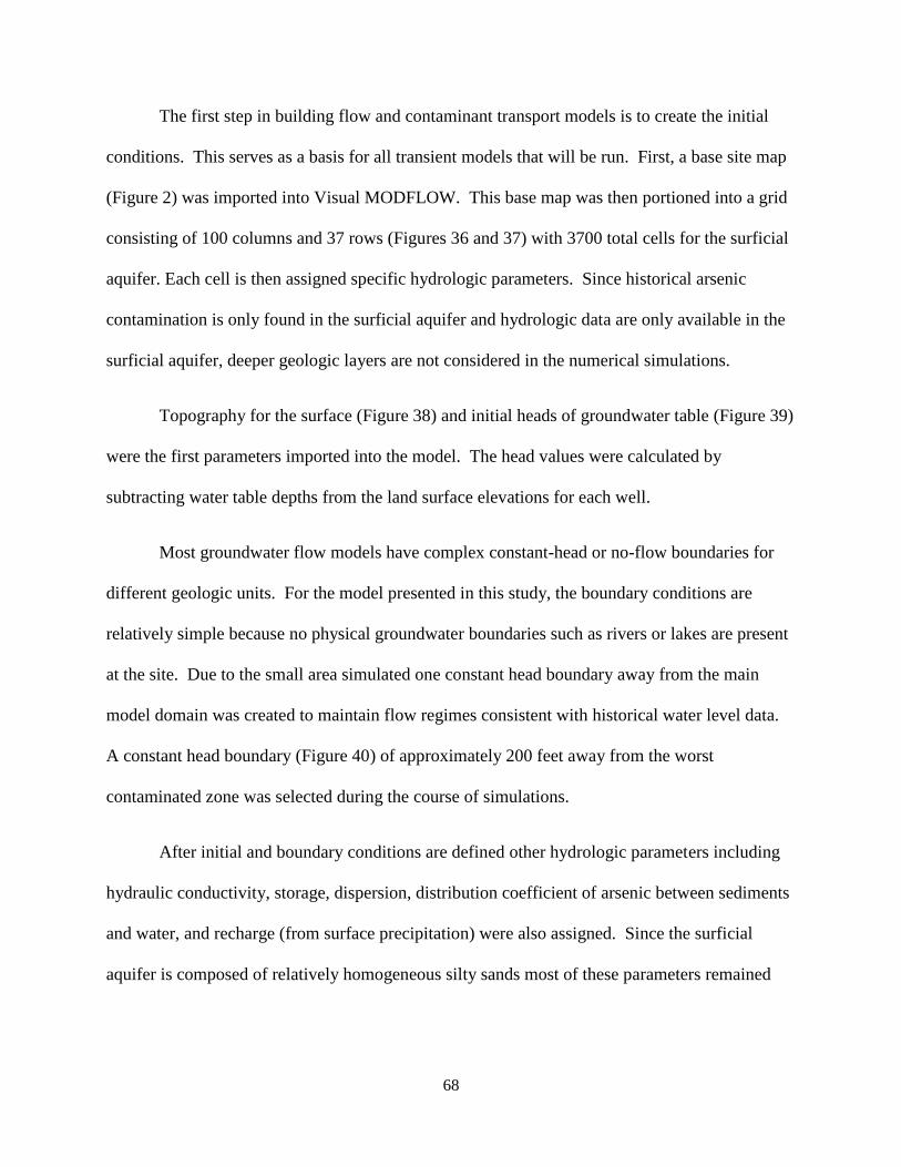
68

The first step in building flow and contaminant transport models is to create the initial

conditions. This serves as a basis for all transient models that will be run. First, a base site map

(Figure 2) was imported into Visual MODFLOW. This base map was then portioned into a grid

consisting of 100 columns and 37 rows (Figures 36 and 37) with 3700 total cells for the surficial

aquifer. Each cell is then assigned specific hydrologic parameters. Since historical arsenic

contamination is only found in the surficial aquifer and hydrologic data are only available in the

surficial aquifer, deeper geologic layers are not considered in the numerical simulations.

Topography for the surface (Figure 38) and initial heads of groundwater table (Figure 39)

were the first parameters imported into the model. The head values were calculated by

subtracting water table depths from the land surface elevations for each well.

Most groundwater flow models have complex constant-head or no-flow boundaries for

different geologic units. For the model presented in this study, the boundary conditions are

relatively simple because no physical groundwater boundaries such as rivers or lakes are present

at the site. Due to the small area simulated one constant head boundary away from the main

model domain was created to maintain flow regimes consistent with historical water level data.

A constant head boundary (Figure 40) of approximately 200 feet away from the worst

contaminated zone was selected during the course of simulations.

After initial and boundary conditions are defined other hydrologic parameters including

hydraulic conductivity, storage, dispersion, distribution coefficient of arsenic between sediments

and water, and recharge (from surface precipitation) were also assigned. Since the surficial

aquifer is composed of relatively homogeneous silty sands most of these parameters remained

69

Fig

ure

35

. A

cro

ss-s

ecti

on s

how

ing c

alcu

late

d r

egio

nal

gro

und

wat

er f

low

reg

ime

in a

of

Bay C

ounty

fro

m w

est

to e

ast.

F

low

was

cal

cula

ted f

rom

the

2D

gro

undw

ater

flo

w m

odel

Bas

in2.

Hydro

stra

tigra

ph

ic f

ram

ework

was

fro

m d

ata

pre

sente

d i

n S

chm

idt

and C

lark

(1980).

A

A’

70

Fig

ure

36

. T

he

Vis

ual

MO

DF

LO

W g

rid d

evel

oped

for

the

Lyn

n H

aven

Ind

ust

rial

sit

e. B

oth

the

x a

nd y

coo

rdin

ates

are

in

met

ers.

A

lso p

lott

ed a

re l

oca

tions

of

sam

ple

d w

ells

.

71

Fig

ure

37

. A

ho

rizo

nta

l tr

anse

ct (

A)

show

ing e

ach c

ell

acro

ss t

he

model

fro

m w

est

to e

ast.

A

ver

tica

l

tran

sect

(B

) sh

ow

ing e

ach

cel

l fr

om

nort

h t

o s

outh

.

A

B

72

Fig

ure

38

. I

mpo

rted

surf

ace

elev

atio

ns

for

the

gro

undw

ater

model

. A

xes

are

in m

eter

s.

73

Fig

ure

39

. T

he

import

ed i

nit

ial

hea

ds

of

the

wat

er t

able

fo

r th

e gro

undw

ater

model

. A

xes

are

in m

eter

s.

74

Fig

ure

40.

Th

e co

nst

ant

hea

d b

oundar

y w

ithin

the

mod

el d

om

ain i

s co

lore

d i

n m

aroon a

nd

is

appro

xim

atel

y 2

00

feet

aw

ay f

rom

the

site

, w

hic

h w

as s

elec

ted n

ot

to i

nte

rfer

e w

ith h

yd

rolo

gic

str

ess

(pum

pin

g a

nd i

nje

ctio

n)

emplo

yed

nea

r th

e m

ajor

arse

nic

plu

me

at s

ite.

75

constant throughout the grid. Values for input parameters (Table 3) were taken from historical

data collected on the site (Mintz and Miller, 1993) or from values recorded during the January

2015 sampling event.

Hydraulic conductivity can be defined as the rate of flow of a volume of groundwater

through a cross section of rock and has dimensions of length/time (Bates and Jackson, 1984). It

is used to show how much water can move through a certain aquifer type per unit time.

Normally, the hydraulic conductivity may vary in different directions. For relatively

isotropic media present at the Lynn Haven industrial site, the geometry of void spaces is assumed

Input Parameter Value

Hydraulic Conductivity 0.0014 cm/s

Specific Storage 9.3 x 10-7 1/m.

Storativity 0.01

Effective Porosity 0.35

Total Porosity 0.35

Dispersivity 10.4 meters

Recharge 66 cm/year

Distribution Coefficient 0; 1; 4; 10 mL/g

Table 3. Values of various hydrologic parameters assigned to the model domain.

76

to be near isotropic and equal in three dimensions (x,y, and z). The hydraulic conductivity for the

surficial aquifer was determined with previous slug testing and was calculated to be 0.0014 cm/s

in all directions (Mintz and Miller, 1993).

The Visual MODFLOW model allows for the use three types of storage parameters:

specific storage (Ss), storativity (S), and porosity (n). Specific storage (Ss) is defined as the

volume of water a unit of volume of aquifer releases from storage under a unit decline in

hydraulic head (Freeze and Cherry, 1979). The unit of specific storage is 1/length.

Storativity (S) is a dimensionless quantity defined as the water released from the

saturated interval of aquifers under per unit decline in hydraulic head, it is calculated by

multiplying an aquifer’s saturated thickness, b, by its specific storage Ss:

S = Ss*b; where

S = storativity

Ss = specific storage

b = thickness of the aquifer

A value of 0.01 was used (Freeze and Cherry, 1979) to specify the storativity of the

unconfined aquifer at the site. The specific storage value of 9.3 x 10-7 1/m was used for the

model (Freeze and Cherry, 1979). Porosity is a measure of percentage of the amount of void

space with a unit volume of aquifer. Effective porosity and total porosity for the surficial aquifer

are assumed to be equal at 0.35 or 35 percent.

Recharge can be defined as the volume of surface water introduced per unit of surface

area of an aquifer through surface infiltration per unit of time. The units for recharge are

77

length/time. For this model cm/year were used from previously published data (Mintz and

Miller, 1993) and recharge for the site is approximately 66 cm/year.

The distribution coefficient Kd can be defined as ratio of sorbed concentration C* of a

contaminant on solids to dissolved contaminant concentration C:

𝐾𝑑 =𝐶∗

𝐶

Thus, larger Kd values indicate that the sorbed concentration of a given contaminant is larger

than the dissolved concentration and vice versa. This parameter controls the extent to which a

dissolved ion can be adsorbed by sediments, which causes the retardation of the solute front as it

travels through an aquifer. The retardation factor Rf is calculated as:

𝑅𝑓 = 1 +𝜌𝑏𝜑𝐾𝑑

Where is b the dry bulk density of the sediment (gm/cm3) and is the porosity of the sediments.

The Kd values for arsenic transport in an aquifer typically range from 1 to 10 mL/g (Allison and

Allison, 2005). If the average linear groundwater flow velocity is v, the average velocity of the

plume vc is given by

𝑣𝑐 =𝑣

𝑅𝑓

The average velocity of a given contaminant plume is lower than that of groundwater because

the value of retardation factor Rf is greater than one. This study used the range of reported Kd

78

values (Allison and Allison, 2005) to assess the impact of adsorption on the movement of arsenic

at the study site.

Groundwater Flow Model

MODFLOW was used to predict changes in hydraulic heads and flow velocities in the

unconfined aquifer at the study site. Water levels measured in all the sampled wells were

selected as the initial condition. Hydrologic parameters used in simulations are shown in Table

3. Figures 41 through 51 show the calculated hydraulic head distribution and flow direction from

the simulations over a period of 10 years. The first time output results presented was 1 day after

the start of the simulation, and then each successive step was one year for 10 years. There are

variations in hydraulic head values of time in the model from the constant recharge that is added

to each cell for each time step. However, the models show that groundwater flows in a general

direction along an east to west-northwest trend over the 10 year simulation span. The predicted

flow direction at local scale is consistent with those predicted in the large regional scale model

near the Lynn Haven site (Figure 35). The predicted flow velocity is on the order of a few to tens

of m per year depending on the local hydraulic gradients.

79

Fig

ure

41

. T

he

sim

ula

ted h

ydra

uli

c hea

d c

onto

urs

and v

eloci

ty a

rro

ws

for

1 d

ay a

fter

the

star

t of

the

model

.

80

Fig

ure

42. T

he

sim

ula

ted h

ydra

uli

c hea

d c

onto

urs

and v

eloci

ty a

rro

ws

for

1 y

ear

afte

r th

e st

art

of

the

model

.

81

Fig

ure

43. T

he

sim

ula

ted h

ydra

uli

c hea

d c

onto

urs

and v

eloci

ty a

rro

ws

for

2 y

ears

aft

er t

he

star

t of

the

model

.

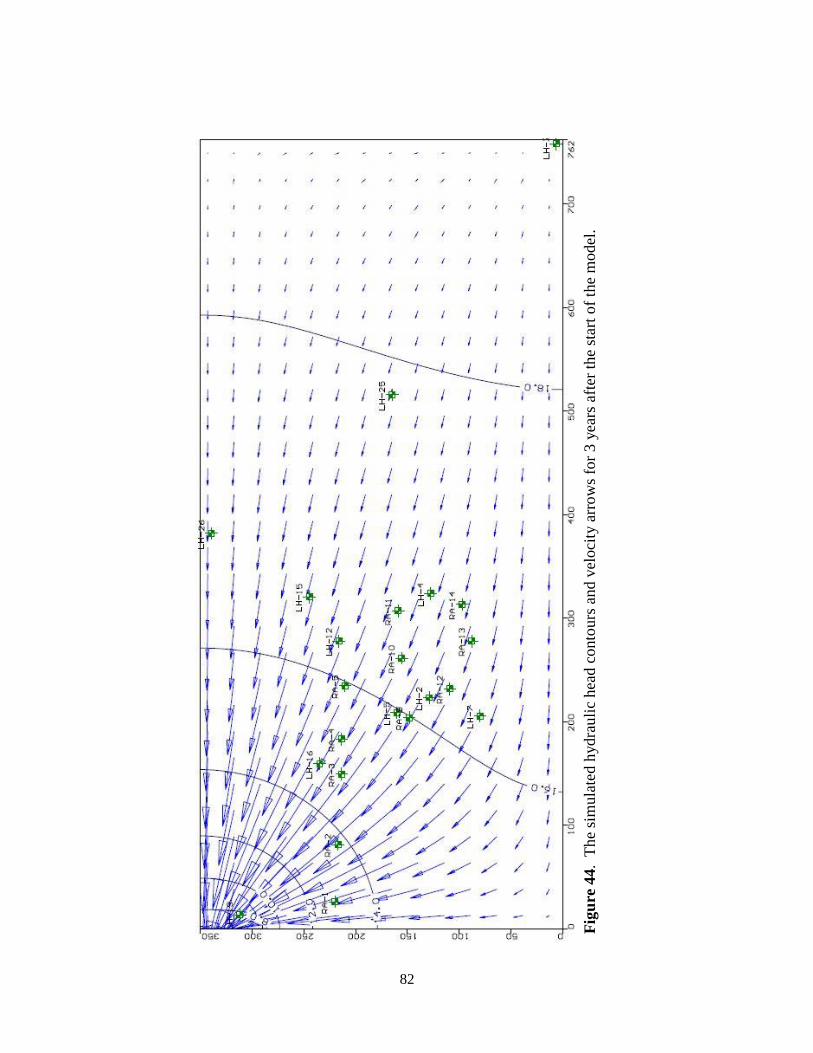
82

Fig

ure

44

. T

he

sim

ula

ted h

ydra

uli

c hea

d c

onto

urs

and v

eloci

ty a

rro

ws

for

3 y

ears

aft

er t

he

star

t of

the

model

.

83

Fig

ure

45. T

he

sim

ula

ted h

ydra

uli

c hea

d c

onto

urs

and v

eloci

ty a

rro

ws

for

4 y

ears

aft

er t

he

star

t of

the

model

.

84

Fig

ure

46. T

he

sim

ula

ted h

ydra

uli

c hea

d c

onto

urs

and v

eloci

ty a

rro

ws

for

5 y

ears

aft

er t

he

star

t of

the

model

.

85

Fig

ure

47. T

he

sim

ula

ted h

ydra

uli

c hea

d c

onto

urs

and v

eloci

ty a

rro

ws

for

6 y

ears

aft

er t

he

star

t of

the

model

.

86

Fig

ure

48. T

he

sim

ula

ted h

ydra

uli

c hea

d c

onto

urs

and v

eloci

ty a

rro

ws

for

7 y

ears

aft

er t

he

star

t o

f th

e m

od

el.

87

Fig

ure

49. T

he

sim

ula

ted h

ydra

uli

c hea

d c

onto

urs

and v

eloci

ty a

rro

w f

or

8 y

ears

aft

er t

he

star

t of

the

model

.

88

Fig

ure

50. T

he

sim

ula

ted h

ydra

uli

c hea

d c

onto

urs

and v

eloci

ty a

rro

ws

for

9 y

ears

aft

er t

he

star

t of

the

model

.

89

Fig

ure

51. T

he

sim

ula

ted h

ydra

uli

c hea

d c

onto

urs

and v

eloci

ty a

rro

ws

for

10 y

ears

aft

er t

he

star

t of

the

model

.

90

Particle Tracking Analysis

Velocity fields calculated from simulated groundwater flow were used in conjunction

with a particle tracking program (MODPATH) to delineate advective transport of contaminants.

Particle tracking simulations predicted flow paths and advective travel distances for specified

periods of time by tracing particle movements through a computed flow field. In this study, a

number of particles were released from two contaminated locations and the advective advance of

those particles through the aquifer was calculated from the simulated flow field over a 10 year

span (Figure 52). The computed flow path of a particle was displayed graphically as a line

connecting trace of discrete points (Figure 52). Results indicate that contaminants such as arsenic

released from the site travel to west or northwest on an average rate of 13 m/year.

MT3DMS (Zheng, 1990) was used to simulate the reactive transport of arsenic at the site

based on flow field and advection process predicted by MODFLOW. Specifically, the model

was used to examine the effect of advection, hydrodynamic dispersion, and adsorption on the

migration of arsenic plumes released from specified locations at the site. The main parameters

influencing solute transport used in simulations are shown in Table 3. The main parameter that

controls the adsorption and retardation of arsenic transport is the distribution coefficient or Kd.

As stated earlier the purpose of these models is to examine the different scenarios of adsorption

for arsenic transportation.

Continuous Contaminant Transport Models

Four continuous contaminant transport models were developed to examine the reactive

transport of arsenic and how the distribution coefficient may affect the spreading of a plume in

the aquifer. All contaminant transport models were run in the groundwater flow fields computed

91

Fig

ure

52. R

esult

s of

par

ticl

e tr

ackin

g i

n V

isual

MO

DF

LO

W. P

arti

cles

wer

e re

leas

ed f

rom

tw

o p

oss

ible

inje

ctio

n s

ites

and t

rack

ed a

s th

ey m

igra

te o

ver

a 1

0 y

ear

of

sim

ula

tion

per

iod

.

92

from transient, three-dimensional numerical models shown in the previous section. For the

simulations, concentration of 4 mg/L of arsenic was specified at a couple cells near its initial

source derived from As-rich pesticides at the site. Sensitivity analyses were conducted to explore

how variations in distribution coefficient Kd values may affect arsenic transport in the aquifer. In

four sets of numerical experiments, the aquifer had constant Kd values of 0, 1, 4, and 10 mL/g,

respectively, close to the range of values reported in literature (Allison and Allison, 2005). The

dispersivity, α, was held constant at 10.4 m (about 10% of the dimension of model domain,

Gelhar et al., 1992) in these simulations. An increase in distribution coefficient would decrease

the extent of arsenic spreading by increasing its sorption on sediments.

This first contaminant model with the Kd value equal to zero mL/g (i.e., no sorption of

the contaminant solution) yielded the greatest degree of spreading and highest arsenic

concentrations downstream, where arsenic is transported at the same rate as groundwater.

Figures 53, 54, and 55 show the movement, size and spreading of the plume 1 day, 1 year, and

10 years after arsenic was released from the source. The size of the initial plume is very small

and restricted to the source area after 1 day due to very limited advection and spreading (Figure

53). After 1 year the zone of maximum contamination or the center of mass of the plume has

started to travel down gradient with the groundwater flow and the overall area of the plume has

grown noticeably by dispersion and spreading (Figure 54). The front of the plume (defined as

0.01 mg/L of concentration) has traveled about 36 meters down gradient. Lastly, after 10 years

the size of the plume has increased significantly and the zone of maximum concentration has

traveled

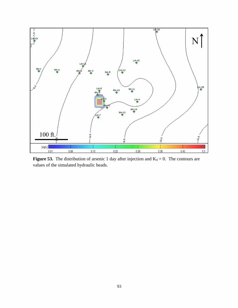
93

Figure 53. The distribution of arsenic 1 day after injection and Kd = 0. The contours are

values of the simulated hydraulic heads.

94

Figure 54. Distribution of arsenic after 1 year with Kd = 0. The contours are the simulated

hydraulic head values.

100 ft.

95

Figure 55. Distribution of arsenic after 10 years with Kd = 0. The contours are the simulated

hydraulic head values.

96

significantly beyond the site toward the west-northwest (Figure 55). The front of the plume has

traveled about 61 meters down gradient.

The second contaminant transport model was run with same parameters as the first. It

contained the same location of injection, but had a larger Kd value of 1 mL/g. The distribution

coefficient used in this model simulated a small amount of arsenic that is being sorbed by the

aquifer sediments. Initially, one day after an injection the plume of contaminant remains close to

the injection location and the zone of maximum contamination is small and restricted to the

source (Figure 56). After 1 year the size of the plume has grown by advection and dispersion

(Figure 57), however it is still smaller than the corresponding plume with Kd equal to zero

(Figure 54). The front of the plume has traveled about 12 meters down gradient, shorter than the

no-adsorption case. After the 10 year simulation the plume is at its largest and is moving in the

north-northwest direction (Figure 58). The size of the plume is still relatively smaller than the

corresponding plume with the Kd equal to zero (Figure 55). The front of the plume has traveled

about 45 meters down gradient after 10 years.

The third contaminant transport model was set up with a higher distribution coefficient

value of 4 mL/g. This value represents stronger adsorption that limits the spreading of the

arsenic plume. Thus, the modeling results show that the plume grows and advances slowly with

time compared to the previous models. The size and distribution of the plume after 1 day is

similar to that of the simulations with lower Kd values. The size and distribution of the plume

after 1 year (Figure 60) has grown little due to strong adsorption and retardation effects. Lastly,

after 10 years the plume is at its largest size and has transported to the west-northwest (Figure

61), but its spreading is very limited compared to other simulations with smaller Kd values. The

front of the plume has traveled about 25 meters down gradient after 10 years.

97

Figure 56. The distribution of arsenic after 1 day with Kd = 1. The contours are the simulated

hydraulic head values.

98

Figure 57. The distribution of arsenic after 1 year with Kd = 1. The contours are the simulated

hydraulic head values.

99

Figure 58. The distribution arsenic after 10 years with Kd = 1. The contours are the simulated

hydraulic head values.

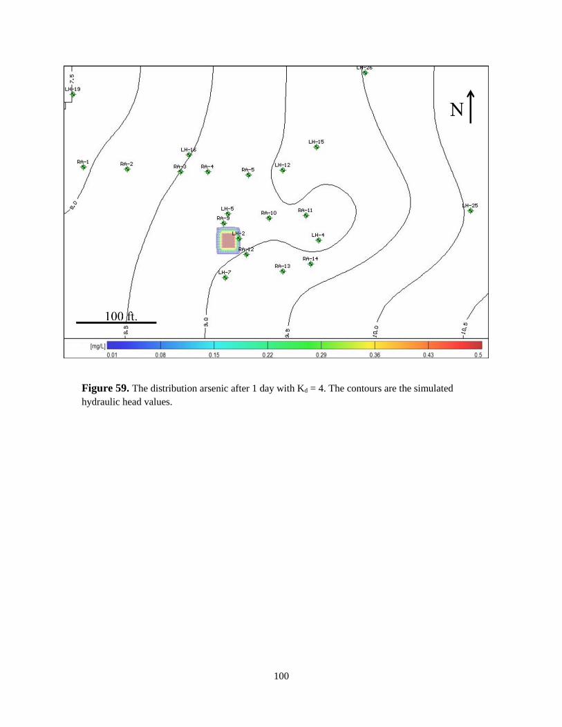
100

Figure 59. The distribution arsenic after 1 day with Kd = 4. The contours are the simulated

hydraulic head values.

101

Figure 60. The distribution arsenic after 1 year with Kd = 4. The contours are the simulated

hydraulic head values.

102

Figure 61. The distribution arsenic after 10 years with Kd = 4. The contours are the simulated

hydraulic head values.

103

In the last model the distribution coefficient was set to a value of 10 mL/g, which is at the

higher end of the spectrum for distribution coefficients expected for arsenic (Figures 62, 63, and

64). The modeling results show the most restricted contaminant transport of among the four

continuous contaminant models. The front of plume has only migrated approximately 15 meters

toward the west from the injection location after 10 years (Figure 64). The advection of the

plume is significantly retarded by strong adsorption and only dispersion leads to limited

spreading from the center of the mass.

Discontinuous Contaminant Transport Models

The discontinuous contaminant transport models were set up in the same manner and

with the same flow parameters as the previous continuous contaminant transport models.

However, the timing of the contaminant injection was reduced from 3650 days (10 years) to just

1 day. This was done to see arsenic transport in the same flow field where the contamination is

an isolated incident that occurs for a very short time period. An observation well located about

12 meters down-gradient from the source was also added to record the breakthrough and

calculated concentration of the traveling plume over time. The distribution coefficients of

arsenic used in the models were 0, 0.5, and 1 mL/g (Figures 65-70).

The first discontinuous transport model was run with a Kd of 0 mL/g. This model

represents how arsenic distribution is affected by an isolated exposure of arsenic without

sorption. In the first year of the simulation the leading edge of the arsenic plume (with As

concentration = 0.01) traveled approximately 24 meters from the source (Figure 65). After 10

years of groundwater flow and recharge, the plume continued to follow the regional flow

direction to the northwest approximately 60 meters offsite (Figure 66).

104

Figure 62. The distribution arsenic after 1 day with Kd = 10. The contours are the simulated

hydraulic head values.

105

Figure 63. The distribution arsenic after 1 year with Kd = 10. The contours are the simulated

hydraulic head values.

106

Figure 64. The distribution arsenic after 10 years with Kd = 10. The contours are the simulated

hydraulic head values.

107

Figure 65. Calculated arsenic distribution for a discontinuous source with a Kd = 0 and 1 year

after introduction. The highlighted cell is the source.

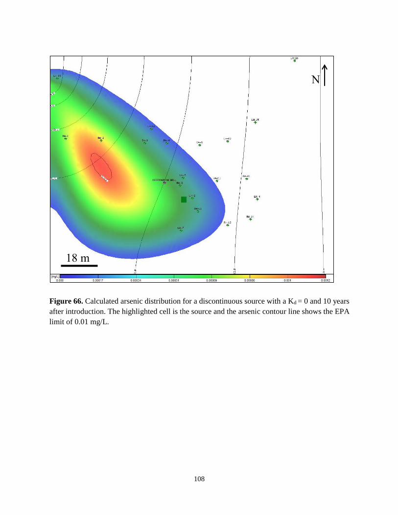
108

18 m

N

Figure 66. Calculated arsenic distribution for a discontinuous source with a Kd = 0 and 10 years

after introduction. The highlighted cell is the source and the arsenic contour line shows the EPA

limit of 0.01 mg/L.

109

N

12 m

Figure 67. Calculated arsenic distribution for a discontinuous source with a Kd = 0.5 and 1

year after introduction. The highlighted cell is the source and the arsenic contour line

shows the EPA limit of 0.01 mg/L.

110

N

12 m

Figure 68. Calculated arsenic distribution for a discontinuous source with a Kd = 0.5 and

10 years after introduction. The highlighted cell is the source and the arsenic contour line

shows the EPA limit of 0.01 mg/L.

111

12 m

N

Figure 69. Calculated arsenic distribution for a discontinuous source with a Kd = 1 and 1

year after introduction. The highlighted cell is the source and the arsenic contour line

shows the EPA limit of 0.01 mg/L.

112

15 m

N

Figure 70. Calculated arsenic distribution for a discontinuous source with a Kd = 1 and

10 years after introduction. The highlighted cell is the source and the arsenic contour

line shows the EPA limit of 0.01 mg/L.

113

The second discontinuous model was run for the same amount of time as the first with a

Kd of 1 mL/g. This model represents an aquifer with a small amount of arsenic sorbed to

sediments. After 1 year the leading edge of the plume traveled approximately 14 meters from

the source (Figure 67). After 10 years the leading edge traveled approximately 50 meters from

the source (Figure 68).

The third discontinuous contaminant transport model was run with the same conditions as

the previous discontinuous models with the exception of distribution coefficient. The Kd used in

this model was equal to 1 mL/g. This represents an aquifer that sorbs arsenic in a 2:1 ratio

compared to the previous case with a Kd value of 0.5 ml/g. After a time of 1 year the plume

traveled approximately 10 meters (Figure 69), which is significantly less than the previous lower

Kd value of 0.5 mL/g. After 10 years the model showed the plume had traveled 37 meters from

the source (Figure 70).

Discontinuous Breakthrough Curves

Plots of calculated arsenic concentrations recorded at the observation well versus time

represent “breakthrough curves” that shows the front, center, and tail of a passing arsenic plume

(Figure 71). Comparing breakthrough curves for the discontinuous shows the effects that Kd has

on the travel time and peak concentration of arsenic plume when it reaches the observation well.

The curve corresponding to Kd = 0 shows that the peak of the arsenic plume took 102 days to

reach the observation well. The curve corresponding to Kd = 0.5 shows that arsenic took 311

days to reach the observation well, and the curve corresponding to Kd = 1 took 1048 days for the

center mass to reach the same destination. The peak concentrations of plumes that reach the

observation well are 0.060, 0.048, and 0.035 ppm for Kd values equal to 0, 0.5, and 1 mL/g,

respectively.

114

0

0.01

0.02

0.03

0.04

0.05

0.06

0.07

0 365 730 1095 1460 1825 2190 2555 2920 3285 3650

Co

nce

ntr

ati

on

(m

g/L

)

Time (Days)

Kd=0

Kd=0.5

Kd=1

Figure 71. Breakthrough curves of calculated concentrations at the observation well

in three discontinuous contaminant transport models.

115

The comparison of the breakthrough curves makes it easy to directly compare the effects

of sorption on contaminant transport in relation to a given point (observation well). The higher

the distribution coefficient (i.e., strong sorption) the longer it takes for the front of the arsenic

plume to reach the well. High Kd values also lead to lower peak concentrations of the plumes.

Proposed Field Biostimulation and Expected Results

The results of the geochemical analyses and modeling suggest that the Lynn Haven

industrial site contains hydrogeochemical conditions that may be amenable for immobilizing or

sequestration of arsenic in groundwater via precipitation of biogenic pyrite. The pump-and-treat

remediation activities have ceased at the Lynn Haven industrial site since the arsenic level has

reduced within 13 to 28 percent of the historical maximum concentration of about 4500 µg/L

(unfiltered). Bacterial sulfate reduction process may potentially provide more cost-effective

solutions for remediating arsenic contaminants in groundwater than traditional pump-and-treat

methods.

XRD and XRF analyses of sediment slurry in the wells show the formation of arsenic-

rich iron sulfide solids, suggesting that sulfate reducing bacteria are removing some arsenic

naturally at the site by precipitating colloidal pyrite, using very limited amount of dissolved

sulfate and organic matter present in the hosting shallow aquifer. Saunders et al. (2005)

performed a similar XRD and geochemical study at this site (Figure 72) and concluded that

bacterial sulfate reduction and precipitation of pyrite were taking place.

The proposed in situ bioremediation approach would require engineering natural SRB

with amendments of organic carbons, nutrients, and iron sulfate to make appropriate biominerals

of Fe-sulfide with high-surface area for arsenic adsorption and co-precipitation (Saunders, 1998;

116

B

A

Quartz

Pyrite

Figure 72. Plot A is an XRD spectrum of aquifer sediments taken from

Saunders et al. (2005). Plot B is an XRD spectrum of aquifer sediments taken

during the January 2015 sampling event. Both plots show sediment from well

RA-5.

Pyrite

Pyrite

Pyrite

Pyrite

Pyrite

117

Saunders et al., 2008; Lutes et al., 2014). After amendments, we expect to see a rapid reduction

in dissolved arsenic concentration once microbial sulfate reduction begins. It should be noted

that injection of organic carbon may initially raise the dissolved Fe and arsenic concentration

(approximately twice the initial level) during the early stage (first few weeks) because it creates

Fe-reducing conditions and mobilizes arsenic from oxides in the aquifer (Saunders et al., 2008).

Once biogenic sulfate reduction begins after about one month of injection, both Fe and As should

decrease dramatically. Late in the experiment, arsenic may return to the background level either

because the sulfate reduction ceases or when the treated groundwater is replaced by surrounding

As-rich groundwater. New injection can proceed in this case to re-establish the sulfate reducing

conditions and form more Fe-sulfide biominerals. Once Fe-sulfide biominerals stabilize in the

aquifer they should continue to remove arsenic by sorption.

118

Conclusions

Geochemical field data and computer modeling techniques were used in this study to

investigate interactions between arsenic-bearing groundwater and its hosting aquifer at the Lynn

Haven industrial site in Bay County, Florida and Macon County, Alabama. The following

conclusions can be made by combining the results of field survey, geochemical analysis, and

numerical modeling.

Observed arsenic concentrations at the Lynn Haven retired substation ranged from

0.0002 ppm to 0.577 ppm in the sampled wells and the average As concentration was calculated

(0.15 ppm) to be well above the EPA standard of 0.01 ppm. Due to the elevated concentrations

of As and past remedial history the most viable option to cost effectively lower As

concentrations is to implement an in-situ bioremediation technology.

The Lynn Haven field site is under moderately reducing conditions, as indicated by

relatively low values of ORP and DO, as well as elevated dissolved sulfide and ferrous iron

concentrations. The main hydrochemical facies of groundwater in the surficial aquifer is

characterized as a Ca-HCO3-Na-Cl type. Na shows largely conservative behavior but a few

samples exhibit slightly enrichment or depletion relative to conservative mixing. Non-

conservative behavior of Na may be explained by Na exchange or fixation on clays.

Groundwater is strongly enriched in Ca and Mg and slightly enriched in K and SO4 relative to

the seawater dilution trend. The enrichment is attributed to a large degree by processes such as

mixing of deeper groundwater from carbonate and clay-rich units as well as ion exchange.

Carbonate rich groundwater would migrate upward into the surficial aquifer in place where the

Jackson Bluff Formation is absent or functions as a semi-confining unit.

119

XRF analyses of selected sediments recovered from both the Macon County and Lynn

Haven sites consistently resulted in major peaks for Fe, S, and As. XRD analyses confirmed the

presence of iron sulfide (pyrite) and arsenic-bearing sulfide minerals. These results suggest that

bacterial sulfate reduction has already led to the sequestration of arsenic in Fe-sulfides at both

sites. The geochemical modeling conducted in this study also suggests that the surficial aquifer

is currently at or near the conditions for sulfate reduction and the precipitation of As-bearing

pyrite. The geochemical modeling results also show the sequence of minerals formed during

bacterial sulfate reduction with a drop in Eh and amendments of FeSO4. Ferrous iron in solution

reacts with sulfide produced from sulfate reduction to form pyrite as the Eh drops below -0.08V.

The precipitation of iron sulfide has the potential to significantly lower the concentration of

arsenic in contaminated groundwater via adsorption and co-precipitation processes.

Results of hydrogeologic modeling with Basin2 and Visual MODFLOW at both

regional and local scales suggest that groundwater and contaminants travel dominantly toward

northwest of the site through time. Groundwater movement is driven by local and regional

topographic relief or water table slope. The calculated flow velocities are on the order of a few to

tens of meters per year. Contaminant transport models (with both continuous and discontinuous

sources) show that the main factors influencing arsenic transport include advection, dispersion,

and adsorption. Varying the distribution coefficient Kd values (1 to 10 ml/g) for different

adsorption models showed that the higher the degree of sorption (high Kd values) the more

arsenic transport is inhibited. Sensitivity analysis shows that adsorption tends to lower the peak

concentration and cause time lag of arsenic transport.

The results of this study also have implications on how to bioremediate the Lynn Haven

site. The geochemical data and modeling suggest that if site conditions are optimized for the

120

stimulation sulfate-reducing bacteria to precipitate iron sulfides, then this may be an effective

bioremedial strategy. When iron sulfides begin to form from the SRB then arsenic will be

adsorbed on to their surface. In order to optimize site conditions soluble sources of organic

carbon, ferrous iron, and sulfate must be injected into the aquifer.

121

References

Allison, J.D., and Allison, T.L., 2005. Partition Coefficients for Metals in Surface Water, Soil,

and Waste: U.S. EPA/600/R-05/074, 93 p.

Appelo, C.A.J., 1994, Cation and proton exchange, pH variations, and carbonate reactions in a

freshening aquifer: Water Resources Research, Vol. 30, No. 10, 13p.

Bates, R.L., and Jackson, J.A., 1984, Dictionary of Geological Terms: New York, Anchor

Books, 571 p.

Bethke, C. M., 2008, Geochemical and biogeochemical reaction modeling. Cambridge

University Press, 543 pp.

Bethke, C.M., M.-K. Lee, H.A.M. Quinodoz, and W.N. Kreiling, 2003, Basin modeling with

Basin2; A guide to using Basin2, B2plot, B2video, and B2view, Hydrogeology Program,

University of Illinois, Urbana.

Charlet, L., and Polya, D.A., 2006. Arsenic in shallow, reducing groundwaters in southern Asia:

an environmental health disaster: Elements 2, 91-96 p.

Cauwenberghe, L., and Roote, D.S., 1998. In Situ Bioremediation: Ground-Water Remediation

Technologies Analysis Center O Series: TO-98-01, 24 p.

122

DeFlaun, M., Lanzon, J., Lodato, M., Henry, S., Onstott, T.E., Chan, E., and Otemuyiwa, B.,

2009, Anaerobic Biostimulation for the In Situ Precipitation and Long-Term

Sequestration of Metal Sulfides: SERDP Project ER1373, 175 p.

Domenico, P.A., and Schwartz, F.W., 1990, Physical and Chemical Hydrogeology: John Wiley

and Sons Inc, 824 p.

Drever, J.I., 1997, The Geochemistry of Natural Waters: 3rd Edition, Prentice Hall, Upper Saddle

River, New Jersey, 436 pp.

Dzombak, D.A., and Morel, F.M., 1990, Surface Complexation Modeling: Hydrous Ferrous

Oxide: John Wiley and Sons, New York, New York, 393 p.

Fetter,C.W. 2001, Applied Hydrogeology, 4th ed., Prentice Hall, Upper Saddle River, NJ, 598 p.

Ford, R.G., Wilkin, R.T., and Puls, R.W., 2007, Monitored Natural Attenuation of Inorganic

Contaminants in Groundwater Volume 2: U.S.EPA/600/R-07/140 108 p.

Frank, J.R., and Peters, R.W. 1992, Remediation of arsenic-oxide contamination: Phase I

groundwater cleanup feasibility – treatability studies: Argonne National Laboratory,

Argonne, Illinois, 19 p.

123

Freeze, A.R., and Cherry, J.A. (1979), Chemical Evolution of Natural Groundwater, In

Groundwater: Prentice Hall, The University of Michigan, pp. 238-289.

Gelhar, L.W., Welty, C., and Rehfeldt, K.R., 1992, A critical review of data on field-scale

dispersion in aquifers: Water Resources Research, 28, 1955-1974 p.

Harvey, C.F., Swartz, C.H., Badruzzman, B., Keon, N.E., Yu, W., Ali, A., Jay, J., Beckie, R.,

Niedan, V., Brabander, D., Oates, P., Ashfaque, K., Islam, S., Hemond, H.F., Ahmed, F.,

2002, Arsenic mobility and groundwater extraction in Bangladesh: Science 298, 1602-

1606 p.

Hem, J.D. (1986), Study and interpretation of the chemical characteristics of natural water, 3rd

ed.: U.S. Geological Survey Water-Supply Paper 2254, 363 p.

Hounslow, A.W., 1980, Groundwater Geochemistry: Arsenic in Landfills: Ground Water 18,

331-333 p.

Huerta-Diaz, M.A., and J.W. Morse. 1992. Pyritization of trace metals in anoxic marine

sediments: Geochimica et Cosmochimica Acta, 56: 2681-2702.

Humayun, M., S.B. Simon, and L. Grossman, 2007. Tungsten and hafnium distribution in

calcium-aluminum inclusions (CAIs) from Allende and Efremovka: Geochim.

Cosmochim. Acta, 71, 4609-4627.

124

Humayun, M., F.A. Davis, and M.M. Hirschmann, 2010. Major element analysis of natural

silicates by laser ablation ICP-MS: J. Anal. At. Spectrom., 25, 998-1005, DOI:

210.1039/C001391A

Keimowitz, A.R., Mailloux, B.J., Cole, P., Stute, M., Simpson, H.J., and Chillrud, S.N., 2007.

Laboratory investigations of enhanced sulfate reduction as a groundwater arsenic

remediation strategy: Environmental Science Technology, 41, 6718-6724

King, D.T., 1994. Upper Cretaceous depositional sequences in the Alabama gulf coastal plain:

Their characteristics, origin, and constituent clastic aquifers: Journal of Sed. Res. B64,

2, 258-265 p.

Korte, N.E., and Fernando, Q., 1991, A Review of Arsenic (III) in Groundwater: Critical

Reviews in Environmental Control 21, 1-39 p.

Lee, M.K., Saunders, J.A., 2003. Effects of pH on metals precipitation and sorption: field

bioremediation and geochemical modeling approaches: Vadose Zone J. 2, 177-185 p.

Lehner, S.W., Savage, K.S., and Ayers, J.C., 2006, Vapor growth and characterization of pyrite

(FeS2) doped with Co, Ni, and As: Variations in semiconducting properties: Journal of

Crystal Growth, 286, 306-317 pp.

125

Lowers, H.A., Breit, G.N., Foster A.L., Whitney, J., Yount, J., Uddin, M.N., and Muneem, A.A.,

2007, Arsenic Incorporation into Authigenic Pyrite, Bengal Basin Sediment, Bangladesh:

Geochimica, Cosmochimica, Acta 71, 2699-2717 p.

Lutes, C., Frizzell, A., Gillow, J., and Beckner, J. (2014), In situ Precipitation of Radionuclides

in Groundwater at US DOE Savannah River Site – 14559: Waste Management

Conference 2014, 14 p.

Markewich, H.W., and Christopher, R.A., 1982. Pleistocene and Holocene fluvial history of

Uphapee Creek, Macon County, Alabama: A paleoenvironmental and paleoclimatic

reconstruction of Holocene sedimentation and incision in an upper coastal plain stream

valley: US Gov. Printing Office, Washington, DC.

McArthur, J.M., Ravenscroft, P., Safiulla, S., and Thirlwall, M.F., 2001, Arsenic in groundwater;

testing pollution mechanisms for sedimentary aquifers in Bangladesh: Water Resources

Research, 37, 109-118 p.

McDonald, M.G., and Harbaugh, A.W., 1988, Techniques of Water Resource Investigations of

the United States Geological Survey, Chapter A1 – A modular three-dimensional finite

difference ground-water flow model: United States Geological Survey Open-File Report

83-875, 484 p.

Mintz, J., and Miller, J., 1993, Lynn Haven Retired Substation Remedial Action Plan: Southern

Company Services, 196 p.

126

Nesbitt, H.W., 1980, Characterization of mineral-solution interactions in Carboniferous

sandstones and shales of the Illinois Sedimentary basin: American Journal of Science, v.

285, 607-630 p.

Nickson, R.T., McArthur, J.M., Ravenscroft, P., Burgess, W.G., and Ahmed, K.M., 2000,

Mechanism of arsenic release to groundwater, Bangladesh and West Bengal: Applied

Geochemistry, 15, 403-413 p.

O’Day, P.O., Vlassopoulos, D., Root, R., and Rivera, N., 2004, The Influence of Sulfur and Iron

on Dissolved Arsenic Concentrations in the Shallow Subsurface under Changing Redox

Conditions: Proceedings of the National Academy of Science, 101, 13703-13708, 6 p.

Penny, E., Lee, M.K., and Morton, C., 2003. Groundwater and microbial processes of the

Alabama coastal plain aquifers: Water Resource Research, 39, 1320. doi:

10.1029/2003WR00196 17 p.

Saunders, J.A., Cook, R.B., Thomas, R.C., and Crowe, D.E., 1996.Coprecipitation of trace

metals in pyrite: Implications for enhanced intrinsic bioremediation: In ed. S.H. Bottrell,

Proc. Fourth International Symposium on the Geochemistry of the Earth’s Surface

(Ilkley, Yorkshire, England), 470-474 p.

Saunders, J.A., Pritchett, M.A., and Cook, R.B., 1997. Geochemistry of biogenic pyrite and

ferromanganese stream coatings: a bacterial connection: Geomicrobiology. J. 14, 203-

217 p.

127

Saunders, J.A., Lee, M.K., Uddin, A., Mohammad, S., Wilkin, R.T., Fayek, M., and Korte, N.E.,

2005, Natural arsenic contamination of Holocene alluvial aquifers by linked linked

tectonic, weathering, and microbial processes: Geochemistry Geophysics Geosystems J.

V.6, 4. doi: 10.1029/2004GC00803.

Saunders, J.A., 2005, Sequestration of Arsenic in Iron Sulfide as a Potential Bioremediation

Technique Using Sulfate Reducing Bacteria: Southern Company Generation Electric

Power Research Institute, 22 p.

Saunders, J.A., Lee, M.K., Shamsudduha, M., Dhakal, P., Uddin, A., Chowdury, M.T., and

Ahmed, K.M., 2008, Geochemistry and mineralogy of arsenic in (natural) anaerobic

Groundwaters: Applied Geochem. 23, 3205-3214 p.

Schmidt, W. and Clark, M.W. 1980, Geology of Bay County, Florida: Florida Geological

Survey Bulletin 57, 96 p.

Shamsudduha, M., Uddin, A., Saunders, J.A., and Lee, M.K., 2008. Quaternary stratigraphy,

sediment characteristics and geochemistry of arsenic-contaminated alluvial aquifers in

the Ganges-Brahmaputra floodplain in central Bangladesh: Journal of Contaminant

Hydrology, 99, 112-136 p.

Smedley, P.L., and Kinniburgh, D.G., 2002, A review of the source, behavior and distribution of

arsenic in natural waters: Applied Geochemistry, 17, 517-568 p.

128

Stueber, A.M., Walter, L.M., Huston, T.J., and Pushkar, P., 1993, Formation waters from

Mississippian-Pennsylvanian reservoirs, Illinois basin, USA: Chemical and isotopic

constraints on evolution and migration: Geochemica et Cosmochemica Acta, v. 57, 763-

784 p.

USEPA, 1995, Contaminants and Remedial Options at Selected Metal-Contaminated Sites:

Washington DC, Office of Research and Development, U.S. Environmental

Protection Agency, EPA/540/R-95/512, 268 p.

USEPA, 1997, Technology Alternatives for the Remediation of Soils Contaminated with As, Cd,

Cr, Hg, and Pb: Washington DC, Office of Emergency and Remedial Response, U.S.

Environmental Protection Agency, EPA/540/S-97/500, 21 p.

USEPA, 2002, Proven Alternatives of Aboveground Treatment of Arsenic in Groundwater:

Washington DC, Office of Solid Waste and Emergency Response, U.S. Environmental

Protection Agency, EPA-542-S-02-002, 68 p.

Veach, O., and Stephenson, L.W., 1911, Preliminary Report of on the Geology of the Coastal

Plain of Georgia: Georgia Geological Survey, Bulletin 26.

Welch, A.H., Westjohn, D.B., Helsel, D.R., and Wanty, R.B., 2000, Arsenic in ground water of

the United States; occurrence and geochemistry: Ground Water, 38, 589-604 p.

Woolson, E.A. (1992), Introduction to arsenic chemistry and analysis, in Abstract Proceedings,

Arsenic and Mercury Workshop on Removal, Recovery, Treatment, and Disposal:

EPA/600/9-92/105.

129

Zheng, C., 1990, MT3D, A modular three-dimensional transport model for simulation of

advection, dispersion, and chemical reactions of contaminants in groundwater systems:

Report to the United States Environmental Protection Agency, Ada Oklahoma, 170 p.