hybrid kalman filter/fuzzy logic based position control of ...cdn.intechweb.org/pdfs/4134.pdf ·...

197

Hybrid Kalman Filter/Fuzzy Logic based Position Control of Autonomous Mobile Robot

Rerngwut Choomuang & Nitin Afzulpurkar Asian Institute of Technology, School of Advanced Technologies, Pathumthani, Thailand

[email protected] [email protected]

Abstract: This paper describes position control of autonomous mobile robot using combination of Kalman filter and Fuzzy logic techniques. Both techniques have been used to fuse information from internal and external sensors to navigate a typical mobile robot in an unknown environment. An obstacle avoidance algorithm utilizing stereo vision technique has been implemented for obstacle detection. The odometry errors due to systematic-errors (such as unequal wheel diameter, the effect of the encoder resolution etc.) and/or non-systematic errors (ground plane, wheel-slip etc.) contribute to various motion control problems of the robot. During the robot moves, whether straight-line and/or arc, create the position and orientation errors which depend on systematic and/or non-systematic odometry errors. The main concern in most of the navigating systems is to achieve the real-time and robustness performances to precisely control the robot movements. The objective of this research is to improve the position and the orientation of robot motion. From the simulation and experiments, we prove that the proposed mobile robot moves from start position to goal position with greater accuracy avoiding obstacles. Keywords: mobile filter, robot, extended Kalman fuzzy logic, obstacle avoidance, stereo vision system.

1. Introduction

Autonomous robot navigation is a popular research area which has still many open problems. There are many attempts to solve the problems related to mobile robot navigation in both known and unknown environments. For the mobile robot navigation system, the motion control is importance for robot navigation. Utilizing the odometry data for motion control, (Johann Borenstein, (1998)) has tested a method called the Internal Position Error Correction (IPEC) for detection and correction of odometry error without inertial or external-reference sensors. Other researchers (Hakyoung Chung & Lauro Ojeda & Johann Borenstein, (2001)) have improved the dead-reckoning accuracy with fiber optic gyroscopes (FOGS) using Kalman filter technique that fuses the sensor data from the FOGS with the odometry system of the mobile robot. An Extended Kalman Filter technique is used for building a localization system (Atanas Georgiev & Peter K. Allen, (2004)). This technique integrates the sensor data and keeps track of the uncertainty associated with it. Authors (W.S. Wijesoma; P.P. Khaw & E.K. Teoh, (2001)) have presented a fuzzy

behavioral approach for local navigation of an autonomous guided vehicle. Distributed sensor-based control strategy for mobile robot navigation has been proposed by (T.M. Sobh; M. Dekhil, A.A. Efros & R. Mihali, (2001)). Authors (Toshio Fukuda; Fellow & Naoyuki Kubota, (1999)) have focused on a mobile robotic system with a fuzzy controller and proposed a sensory network that allows the robot to perceive its environment. For obstacle avoidance in mobile robot navigation, authors (Alexander Suppes; Frank Suhling & Michael Hotter, (2001)), have proposed an approach using video based obstacle detection for a mobile robot based on probabilistic evaluation of image data. Obstacle detection is realized by computing obstacle probability and subsequent application of a threshold operator. They also identified other types of systematic error and non-systematic error related to the mobile robot’s motion such as odometry error due to inadequate encoder resolution, unequal wheel diameter, orientation error due to presence of slippage, angular velocity error of the gyroscope, floor, etc. The organization of the paper is as follows: section 2 presents a brief description of navigation system of

Choomuang, R. & Afzulpurkar, N. / Hybrid Kalman Filter/Fuzzy Logic based Position Control of Autonomous MobileRobot, pp. 197 - 208, International Journal of Advanced Robotic Systems, Volume 2, Number 3 (2005), ISSN 1729-8806

198

elaborated of fusing together mobile robot developed as part of this research. The proposed approach to solve the robot motion problem is in section 3. In section 4 and 5, we describe the methodology Extended Kalman Filter, Fuzzy Logic Control, and Obstacle Avoidance techniques to implement the proposed system including hardware and software realization. The experimental results are shown in section 6. Conclusion and future research direction are given in section 7.

2. Mobile robot navigation techniques

The dead-reckoning principle has been used as standard technique navigation for mobile robot positioning. The fundamental idea of dead reckoning is based on a simple mathematical procedure for determining the present location of the robot by advancing previous position through known course and velocity information over a given length of time (H.R. Everett, 1995). This allows for used of measured wheel revolutions to calculate displacement relative to floor. The advantage of odometry is that it provides good short-term accuracy and allows very high sampling rates.

2.1 Kalman FilterKalman filter (KF) is widely used in studies of dynamic systems, analysis, estimation, prediction, processing and control. Kalman filter is an optimal solution for the discrete data linear filtering problem. KF is a set of mathematical equations which provide an efficient computational solution to sequential systems. The filter is very powerful in several aspects: It supports estimation of past, present, and future states (prediction), and it can do so even when the precise nature of the modeled system is unknown. The filter is derived by finding the estimator for a linear system, subject to additive white Gaussian noise (Ashraf Aboshosha, 2003). However, the real system is non-linear, Linearization using the approximation technique has been used to handle the non-linear system. This extension of the non-linear system is called the Extended Kalman Filter (EKF). The general non-linear system and measurement form is as given by equation (1) and (2) as follows:

),;,( 111 −−−= kkkkk wuxfx γ (1) );( kkk vxhz = (2)

where kx is a state vector and kz is a measurement vector at the time k, )(⋅f and )(⋅z are non-linear system and measurement function, ku is input to the system,

kw , kγ and kv are the system, input and measurement noises respectively.. ),0(~ QNwk , ),0(~ ΓNkγ and

),0(~ RNvk indicate a Gaussian noise with zero mean and covariance matrix Q , Γ and R (Evgeni Kiriy & Martin Buehler, 2002).

The main operation of Extended Kalman Filter is divided into two parts, the prediction part and the correction part.

1. Prediction part: This part of the EKF predicts the future state of the system −

kx̂ and projects ahead the

state error covariance matrix −kP using equation (3)

and (4) as:

)0,0;,(ˆ 1 kkk uxfx −− = (3)

11 −−− +Γ+= k

Tkk

Tkkkk QBBAPAP (4)

2. Correction part: This part performs the measurement update using equation (5), (6) and (7) as shown below:

1)( −−− += kTkkk

Tkkk RHPHHPK (5)

))0,ˆ((ˆˆ −− −+= kkkkk xhzKxx (6) −−= kkkk PHKIP )( (7)

where I is an identity matrix and system (A), input (B), and measurement (H) metrics are calculated by Jacobians of the system )(⋅f and measurement )(⋅h (Evgeni Kiriy & Martin Buehler, 2002) using equations (8), (9) and (10).

)0,0;,ˆ(][

][],[ kk

j

iji ux

xf

A −

∂∂

= (8)

)0,0;,ˆ(][

][],[ kk

j

iji ux

yf

B −

∂∂

= (9)

)0;ˆ(][

][],[

−

∂∂

= kj

iji x

xh

H (10)

2.2 Fuzzy Logic ControlThe idea of fuzzy sets was proposed by Lofti A. Zadeh in July 1964. The Fuzzy Logic can be used for controlling a process (i.e., a plant in control engineering terminology) which is non-linear, the advantage of Fuzzy logic control is that it enables control engineers to easily implement control strategies which can be used by human operator. Its core technique is based on four basic concepts: fuzzy sets, linguistic variables, possibility distributions and fuzzy if-then rule (John Yen & Reza Langari, 1999). Fuzzy logic has been applied to various control system. The block diagram of fuzzy logic controller shown in Fig. 1 is composed of the following four elements (Kevin M. Passino & Stephen Yurkovich, 1998):

1. A rule-base (a set of If-Then rules), which contains a fuzzy logic quantification of the expert’s linguistic description of how to achieve good control.

2. An inference mechanism (also called “inference engine” or “fuzzy inference” module), which emulates the expert’s decision making in interpreting and applying knowledge about how best to control the plant.

3. A fuzzification interface, which converts controller inputs into information that the inference mechanism can easily use to activate and apply rules.

199

4. A defuzzification interface, which converts the conclusions of the inference mechanism into actual inputs for the process.

Fuzzy Logic Controller

Fuzz

ifica

tion

Def

uzzi

ficat

ionInference

mechanism

Rule-base

Inputsu(t)

Reference inputr(t)

Outputsy(t)Process

Fig. 1. The block diagram of fuzzy logic control system

2.3 Stereo Vision System The basic idea of a typical stereo vision system is to find corresponding points in stereo images and infer 3D knowledge about the environment. Corresponding points are the projections of a single 3D point in the different image spaces. The difference in the position of the corresponding points in their respective images is called disparity (Marti Gaëtan, 1997). The ideal situation is illustrated in Fig. 2. An arbitrary point in a 3-D scene is projected into different locations in stereo images.

Rz

Rx

Ry

Lz

Lx

Ly

Lo Ro

b

),,( zyxP

LP RP

Fig. 2. A typical 3-D scene projected in stereo images

Assume that a point P in a surface is projected onto two cameras image planes, PL and PR, respectively. When the imaging geometry is known, the disparity between these two locations provides an estimate of the corresponding 3-D position. Specifically, the location of P can be calculated from the known information, PL and PR, and the internal and external parameters of these two cameras, such as the focal lengths and positions of two cameras. Shown in Fig. 2 is a parallel configuration, where one point, p(x,y,z), is projected onto the left and right of the imaging planes at PL(xl,yl) and PR(xr,yr),respectively. The coordinates of P can be calculated (Jung-Hua Wang & Chih-Ping Hslao, 1999) using equation (11) as follow:

−−+

−+

=)(

,)(2)(

,)(2)(

),,(rlrl

rl

rl

rl

xxbf

xxyyb

xxxxb

zyxP (11)

where (xl -xr) is the disparity, base line b is the distance between the left and right cameras, and f is the focal length of the camera

3. Proposed mobile robot design and motion control system

3.1 The motion control problem In most robot’s motion, it is very likely that there are positioning problems when the robot moves from a starting position to a goal position. This error may include the orientation error due to slippage during the move. Assume R to be a robot, this robot starts from an initial position P0 to the goal position Pg in an unknown workspace. Let O be an obstacle in the required workspace W. During a robot move from current position Pk to the next position Pk+1, there is a change in the position and/or orientation. This change causes accuracy problem the robot’s location from in calculating current position to next position. The new location is not a verified true position. The position error increases as the robot keeps moving as shown on Fig. 3.

00 ,θP 11,θP

22 ,θP

22 ,θP ggP θ,

kkP θ,

Obstacle

Fig. 3. Typical robot move

3.2 New mobile robot platform design A mobile robot has been developed in this research, as shown in Fig. 4 and Fig. 14a . It was built on a circular platform with three-wheel configuration. The robot has a diameter of 340 mm and a height of 170 mm. It consists of two driven wheels in the front and single passive wheel in the rear. An optical encoder is mounted on the axis of each wheel used for the odometry measurement.

120

mm5.92

mm10

mm240

Motor Motor

EncoderEncoder

sensorposition

Bettery

boardControllerMotion

wheelPassive

wheelDriving

mm208

Fig. 4. Schematic diagram of the mobile robot

200

Three separate modules are used external sensors. A vector compass module which is attached to the middle of the robot’s chassis to measure the robot heading. A position sensor module which is placed underneath robot chassis 3 mm above the floor to provide the robot position. The last module, the vision sensor is placed on top of the upper circular platform of the mobile robot to provide the stereo vision capability to the robot.

3.3 Motion control architecture The proposed mobile robot controller is actually a small computer network consisting of an embedded PC (a PC104) and two microcontrollers (DS89C420). All of them are connected together as show in Fig. 5.

Microcontroller I Microcontroller II

En1

Stereo VisionSensor

VectorCompassPosition sensor

Master Controller

En2M1 M2

Velocity(PWM signal)

COM 1 COM 2IEEE 1394

8-BIT dataLEAD/LAG

PULSE

X-Axis(LEAD/LAG)

PULSE

Y-Axis(LEAD/LAG)

PULSE

Fig. 5. Network architecture of the robot

The PC104 is the master controller for the mobile robot, it controls all the activities of two slave controllers (DS89C420s). On a typical robot command, the master controller collects the following information from the Microcontrollers,: optical encoder feedback data from both wheels, robot heading data from vector compass module and absolute position from position sensor module. The slave controllers also act as protocol converters. This eliminates all the protocol conversion burden for the Master controller and allows the PC104 to concentrate only on the necessary control calculations. Table 1. provides typical protocol conversion burden times for each microcontroller. With this approach, the maximum time for updating the position control command is approximately 8 milliseconds. The motor response time is set at 20 milliseconds interval. As mentioned before there are 4 sensors mounted on the mobile robot: vector compass, wheel encoder, position sensor and vision sensor.

PC104 protocol’s

burden time

No. of protocol bytes

Baud rate

Microcontroller I 5 ms 5 9600 Microcontroller II 1 ms 1 9600

Table 1. Typical protocol burden’s time between PC104 and Microcontrollers

The detail characteristics of sensors are follows:

• Vector compass: this is an electronic compass module with a resolution of 0.1 degree (more resolution is also possible with appropriate hardware and software configurations). Appropriate calibrations techniques provided by the manufacturer cancle out the errors due to variation of the local geomagnetic field and geographic north effects.

• Wheel encoder: each wheel of the mobile robot is equipped with an optical encoder (with 200 counts per revolution). This allows each axis to provide separate wheel’s information independently and accurately. The speed of the motor is set at 50 revolutions per minute, with this speed, the time interval between each encoder pulse is 100 microseconds.

• Position sensor: this is an electronics sensor based on encoder circuit, to provide direction and counts on 2 linear axes (x-axis and y-axis). The normal resolution is 400 counts/inch (with a maximum resolution of 800 counts/inch). This is an attempt to minimize the computation due to translation during the robot movement.

• Stereo vision sensor: this is a vision sensor which consists of a two-camera module (The Digiclops™ Stereo Vision camera) to perform range measurements for sensing the environment. It is possible to determine the distance to points in the scene reliably in a range from 0.5 to 6.0 meters.

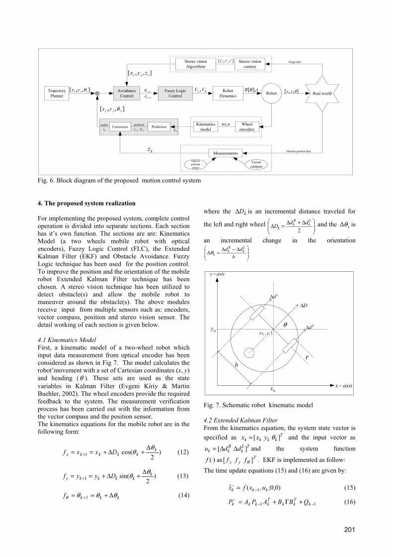
3.4 Proposed motion control algorithm Fig. 6 shows a block diagram for our proposed motion control system. In the proposed algorithm stereo vision is used to calculate the 3D position of obstacles in the robot path. Extended Kalman Filter, Fuzzy Logic technique and Obstacle avoidance have been implemented in the proposed new motion control system (including information from various sensors). The proposed algorithm has improved the robot’s movement as well as the robot’s position and orientation. The operation of the proposed motion control algorithm can be summarized as follows:

1. Set the start and goal position. 2. Check obstacles in front of the robot using stereo

vision sensor. If the robot finds an obstacle, then it computes the avoidance angle or/and the remaining distance to the goal.

3. After the robot has computed the angle error and the distance error in step 2, robot then calculates a set of velocity of the left and the right wheels using the Fuzzy Logic technique.

4. While the robot moves, it verifies a motion’s information from the existing internal and external sensors. The Extended Kalman Filter is activated for the robot’s motion.

5. If robot does not reach the required goal position, the algorithm step 2 is repeated.

201

TrajectoryPlanner

Fuzzy LogicControl Real worldRobotAvoidance

Control

Wheelencoders

Kinematicsmodel

],,[ rrr yx θ

],,[ fff yx θ

],,[ vvv zyx

ω,dΔ

error

error

dθ Robot

DynamicsRL VV , tR ),(θ

Stereo visioncamera

Stereo visionAlgorithms

Measurements

Vectorcompass

Opticalpositionsensor

PredictionCorrectionkx

kz

−+

−+ 11 ,ˆ kk Pxkx̂

predicted

Image data

update

]',','[ zyx

Absolute position data

],,[ θyx

Fig. 6. Block diagram of the proposed motion control system

4. The proposed system realization

For implementing the proposed system, complete control operation is divided into separate sections. Each section has it’s own function. The sections are are: Kinematics Model (a two wheels mobile robot with optical encoders), Fuzzy Logic Control (FLC), the Extended Kalman Filter (EKF) and Obstacle Avoidance. Fuzzy Logic technique has been used for the position control. To improve the position and the orientation of the mobile robot Extended Kalman Filter technique has been chosen. A stereo vision technique has been utilized to detect obstacle(s) and allow the mobile robot to maneuver around the obstacle(s). The above modules receive input from multiple sensors such as: encoders, vector compass, position and stereo vision sensor. The detail working of each section is given below.

4.1 Kinematics Model First, a kinematic model of a two-wheel robot which input data measurement from optical encoder has been considered as shown in Fig 7. The model calculates the robot’movement with a set of Cartesian coordinates (x, y)and heading (θ ). These sets are used as the state variables in Kalman Filter (Evgeni Kiriy & Martin Buehler, 2002). The wheel encoders provide the required feedback to the system. The measurement verification process has been carried out with the information from the vector compass and the position sensor. The kinematics equations for the mobile robot are in the following form:

)2

cos(1k

kkkkx Dxxfθ

θΔ

+Δ+== + (12)

)2

sin(1k

kkkky Dyyf θθ Δ+Δ+== + (13)

kkkf θθθθ Δ+== +1 (14)

where the kDΔ is an incremental distance traveled for

the left and right wheel Δ+Δ=Δ2

Lk

Rk

kddD and the kθΔ is

an incremental change in the orientation Δ−Δ

=Δb

dd Lk

Rk

kθ

θ

mx

my

br

LdΔ

RdΔ

DΔ

axisy −

axisx −

),( rr yx

Fig. 7. Schematic robot kinematic model

4.2 Extended Kalman Filter From the kinematics equation, the system state vector is specified as T

kkkk yxx ][ θ= and the input vector as TL

kRkk ddu ][ ΔΔ= and the system function

)(⋅f as Tyx fff ][ θ . EKF is implemented as follow:

The time update equations (15) and (16) are given by:

)0,0;,(ˆ 1 kkk uxfx −− = (15)

11 −−− +Γ+= k

Tkk

Tkkkk QBBAPAP (16)

202

where kA and kB are the Jacobian matrix of the system and input matrix respectively are obtained by linearization as shown in equation (17) and (18) (Evgeni Kiriy & Martin Buehler, 2002).

Δ+Δ

Δ+Δ−

=

∂∂

∂∂

∂∂

∂∂

∂∂

∂∂

∂∂

∂∂

∂∂

=

100

)2

cos(10

)2

sin(01

kkk

kkk

kkk

k

y

k

y

k

y

k

x

k

x

k

x

k

D

D

fyf

xf

fyf

xf

fyf

xf

A

θθ

θθ

θ

θ

θ

θθθ (17)

Δ+

Δ+

Δ+

Δ+

Δ−

Δ+

−

Δ+

Δ−

Δ+

Δ+

Δ+

Δ+

=

Δ∂∂

Δ∂∂

Δ∂

∂

Δ∂

∂Δ∂∂

Δ∂∂

=

b

bDb

Db

bDb

D

Df

Df

D

f

D

fDf

Df

B

kk

kkk

kk

kkk

kk

kkk

kk

kkk

Rk

Lk

Rk

yLk

y

Rk

xLk

x

k

1

)2

cos(2

)2

sin(21

)2

sin(2

)2

cos(21

1

)2

cos(2

)2

sin(21

)2

sin(2

)2

cos(21

θθθθ

θθθθ

θθθθ

θθθθ

θθ

(18)

For the measurement update, the Jacobian of the function T

kkk yxh ][)( θ=⋅ , measurement matrix kH is represented in equation (19) as:

=

∂∂

∂∂

∂∂

∂∂

∂∂

∂∂

∂∂

∂∂

∂∂

=100010001

kkk

k

y

k

y

k

y

k

x

k

x

k

x

k

hyh

xh

hyh

xh

hyh

xh

H

θ

θ

θ

θθθ

(19)

The measurement update equations are given by (Evgeni Kiriy & Martin Buehler, 2002):

1)( −−− += kTkkk

Tkkk RHPHHPK (20)

))0,ˆ((ˆˆ −− −+= kkkkk xhzKxx (21) −−= kkkk PHKIP )( (22)

With these set of equations all the necessary components of EKF have been defined.

4.3 Fuzzy Logic Control The objective to use the Fuzzy Logic Control is to generate the velocities for both the left and the right motors of the robot, which allows the robot to move from start position to goal position. The specification of the control input and output variables have been set. These inputs are: angle errorθ which is the difference between

the goal angle gθ and the current heading rθ of robot, the distance errord which is the difference between the current position and the goal position. The calculation is a simple computation of the basic equation between two points. The outputs of Fuzzy Logic Controller are velocities of the left and right motors of the mobile robot. Fig. 8 shows the proposed Fuzzy Logic Controller block diagram.

Fuzzy ofmotor left

Fuzzy ofmotor right

errorθ

errordLv

Rv

Fuzzy Logic Controller

motorleft

motorright

encoder

encoder

drivecontrol

drivecontrol

refv

refv

fv

fv

v

v

Fig. 8. Schematic diagram for the proposed fuzzy logic controller

Fuzzy logic technique has been used to generate the velocities for each motor of the two wheel mobile robot. The fuzzy logic algorithm is as follows:

Step 1: Define the linguistic variable(s) for input and output system

• Compute two input variables: angle error (the different angle between goal angle and robot’s heading) and distance error (the difference between the current position and goal position). Compute two output variables: the velocities of the left and right motors.

Step 2: Define fuzzy set • The fuzzy set values of the fuzzy variables are

divided as shown in the Table 2. • The fuzzy set values are set of overlapping

values represented by triangular shape that is called the fuzzy membership function. Typical representations of the fuzzy membership function are shown in Fig. 9, Fig. 10 and Fig. 11 below.

Angle: θerror Distance: derror

NL: Negative Large Z: Zero NM: Negative Middle N: Near NS: Negative Small M: Middle ZE: Zero F: Far PS: Positive Small PM: Positive Middle PL: Positive Large

Table 2. Notations for the Fuzzy Logic

90604020090− 60− 40− 20−

PLPMPS

ZE

NSNMNL

Fig. 9. Representation of the fuzzy membership functions of angle error

203

100100− 20 40 60 800

FSFW

S

FSBW BW SLBW SLFW FW

80− 60− 40− 20−

Fig. 10. Representation of the fuzzy membership functions of velocity output

ZN M F

1 2 4 5 m0 3

Fig. 11. Representation of the fuzzy membership functions of distance error

Step 3: Define fuzzy rules • The operation of the system utilizes the fuzzy

rules. The notation for making fuzzy logic rules is: Fast Forward (FSFW), Forward (FW), SlowForward (SLFW), Stop (S), Slow Backward(SLBW), Backward (BW) and Fast Backward (FSBW). The fuzzy rules are shown in the Table 3. and 4. below

Z N M F NM S FSFW FSFW FSFW NM S FW FW FW NS S SLFW FW FW ZE S SLFW FW FSFW PS S S SLFW SLFW PM S S SLFW SLFW PL S S FW FW

Table 3. Fuzzy rule of the right motor

Z N M F NM S S BW BW NM S S SLBW SLBW NS S S SLBW SLBW ZE S SLBW BW FSBW PS S SLBW BW BW PM S BW BW BW PL S FSBW FSBW FSBW

Table 4. A typical fuzzy rule of the left motor

Examples of fuzzy rule employed by the path following behavior are shown below:

1ℜ : IF θerror is zero angle (ZE) and derror is distance near (N) THEN the left motor is Slow Backward (SLBW)

2ℜ : IF θerror is zero angle (ZE) and derror is distance near (N) THEN the right motor is Slow Forward (SLFW)

Step 4: Defuzzification • The output action given by the input conditions,

the defuzzification computes the velocity output of the fuzzy controller.

• Centroid defuzzification or Center of Area method calculated by equation (23) as:

=

=

×

=n

i

dii

dii

n

ii

errorerror

errorerrorvv

1

1

),min(

),min(

μμ

μμ

θ

θ

(23)

where v is defined the fuzzy output of thi rule, erroriθμ

and errordiμ are the membership value of the input fuzzy

set

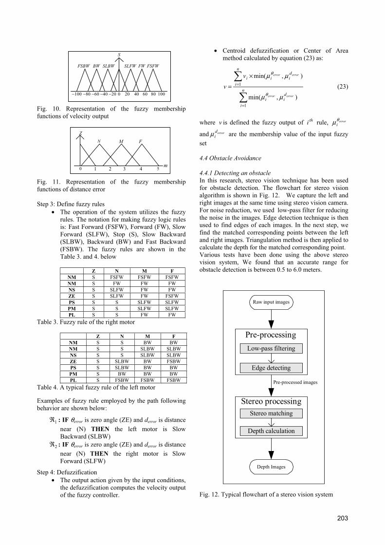
4.4 Obstacle Avoidance

4.4.1 Detecting an obstacle In this research, stereo vision technique has been used for obstacle detection. The flowchart for stereo vision algorithm is shown in Fig. 12. We capture the left and right images at the same time using stereo vision camera. For noise reduction, we used low-pass filter for reducing the noise in the images. Edge detection technique is then used to find edges of each images. In the next step, we find the matched corresponding points between the left and right images. Triangulation method is then applied to calculate the depth for the matched corresponding point. Various tests have been done using the above stereo vision system, We found that an accurate range for obstacle detection is between 0.5 to 6.0 meters.

Pre-processed images

Low-pass filtering

Edge detecting

Pre-processing

Depth calculation

Stereo matching

Stereo processing

Raw input images

Depth Images

Fig. 12. Typical flowchart of a stereo vision system

204

The algorithm for obstacle detection is as follows:

endreturn

sobstaclefoundnotelse

zyxreturnsobstaclefound

thendanddIf

obsobsobs

obsobs

)0,0,0()(

),,()(

0.65.0 ≤≥

where obsd is the distance between the robot and the obstacle.

4.4.2 Avoiding an obstacle To avoid the existing obstacles, a series of movement commands must be generated to allow the mobile robot to move pass the obstacles. In order to do so, the program within the mobile robot must analyze the incoming coordinates from 4.4.1. Additional data such as the obstacle angle θobs is calculated which eventually lead to the calculation avoidance angle avoidθ for the mobile robot to move through the detected obstacles.

rθ dθ

gθ

Obstacle

Goal

),( obsobs yx

),( gg yx

axisx −

axisy −

),( 00 yx

axisx −'

axisy −'

gd

),( rr yx

obsd

obsθ

Fig. 13. Schematic for obstacle avoidance

The angle θd is the difference between the heading angle θr and the obstacle angle θobs . It’s calculated by equation (24) as follow:

obsrd θθθ −= (24)

Avoiding angle, θavoid is then calculated as:

end

else

thenif

obsgavoid

obsgavoid

d

θθθ

θθθθ

+=

−=< 0

The equations for inputs to the Fuzzy Logic control are as follow:

avoidrerror θθθ −= (25)

22 )()( rgrgerror yyxxd −+−= (26)

where errorθ is error angle for input fuzzy logic, errord is error distance for inputs to fuzzy logic, obsθ is an obstacle angle, avoidθ is avoiding angle, gθ is goal angle,

rθ is the heading of the mobile robot, ),( gg yx is a

destination position, and ),( rr yx is a current position of the robot.

To improve the precision in the motion control of the robot motion, Extended Kalman Filter, the Fuzzy Logic control and the obstacle avoidance techniques have been implemented. We present the results from the experiments in section 6 to validate the above algorithms.

5. Hardware and software implementation

To test the proposed algorithms, a mobile robot which corresponds to the schematic design has been constructed and is shown in Fig. 4 and Fig 14a. The maximum speed of the robot is approximately 0.45 meters per second. The interfacing circuit of the velocity controller which receives signals from the wheel encoder is shown in Fig. 14a. The interfacing circuit in Fig. 14b also receives signals from the vector compass and the position sensor. In both cases, the DALLAS 89C420 microcontroller has been used. The software interface for the DALLAS 89C420 microcontrollers and sensor module has written in assembly language (MCS-51 family instruction). Software interface for the stereo camera module is written in Microsoft Visual C++ (using vision library from the Point Grey Company). The simulation program is written using MATLAB.

Fig. 14a. An experimental mobile robot

DS89C420

CompassVector

SensorPosition

0INT1INT2INT3INT

0.0P1.0P

3.0P4.0P5.0P

2.0P

6.0P7.0P

TXRXGND

298L

1M

2M

INAINBINCIND

OUTA

OUTBOUTC

OUTD

1EN2EN

0074LS

CHA

CHB

CHA

CHB

1PWM2PWM

1DIR2DIR

DS89C420

0.0P1.0P2.0P3.0P

0INT1INT

0.1P1.1P

TXRXGND

)(a )(b

Fig. 14b. Interface circuit for the mobile robot controller

205

6. Experimental results

The mobile robot with the proposed algorithm has been tested in various unknown environments with obstacles. In all experiments, the robot moved from the start positions to the goal positions correctly and the rest of this section provides results form the simulation experirments performed using the above control algrothm

6.1 Simulation Results The simulations were performed using different maps consisting goal and obstacles.

x[mm]

y[mm]

50 100 150 200 250 300 350 400

50

100

150

200

250

300

350

400

Obstacle 2

Obstacle 1

Obstacle 3

Start(30,200) Goal(350,200)

Fig. 15a. The trajectory of the robot movement

0 50 100 150 200 250 300 350 400196

198

200

202

204

206

208

210

212

214Position of x

x[mm]

y[mm]

True positionFLCFLC & EKF

Fig. 15b. The comparison of robot motion in xy-axis using only FLC and FLC & EKF

0 0.5 1 1.5 2 2.5 3 3.5 4 4.5 5196

198

200

202

204

206

208

210

212

214Position of y

time[sec]

y[mm]


Fig. 15c. The comparison of robot motion in y-axis using FLC and FLC & EKF

0 0.5 1 1.5 2 2.5 3 3.5 4 4.5 5-0.8

-0.6

-0.4

-0.2

0

0.2

0.4

0.6Heading of robot

time[sec]

theta[rad]


Fig. 15d. The comparison of robot heading using FLC and FLC & EKF

x[mm]

y[mm]

50 100 150 200 250 300 350 400

50

100

150

200

250

300

350

400

Start(30,200)

Obstacle 2

Obstacle 3

Goal(350,220)

Obstacle 1


0 50 100 150 200 250 300 350 400190

195

200

205

210

215

220

225Position of x

x[mm]

y[mm]



Fig. 15a to show the trajectory followed by the robot avoiding an obstacle on the left hand side of the robot. The simulation results are shown in Fig. 15b, Fig. 15c and Fig. 15d respectively. The “ −•− ” represents the true position/orientation of the robot motion, the “ −Δ− ”represents trajectory after the position/orientation error are compensated using the fuzzy logic technique and the “ −−o ” represents the trajectory after position/orientation errors are compensated by the Kalman Filter and Fuzzy Logic techniques. Fig. 16 and Fig. 17 show similar experiments using other maps. Second simulation experiment (Fig. 16a) has three

206

obstacles in the workspace. The robot moves from start position (30,200) to destination position (350,220). The results changes of xy-position, y-position and heading of robot are show in Fig. 16b, Fig. 16c and Fig. 16d respectively.

0 1 2 3 4 5 6195

200

205

210

215

220Position of y

time[sec]

y[mm]



0 1 2 3 4 5 6-0.8

-0.6

-0.4

-0.2

0

0.2

0.4

0.6Heading of robot

time[sec]

theta[rad]



Third simulation experiment, the robot moves from the start position (30,200) to destination position (350,260) by the workspace has seven obstacles (Fig. 17a). Fig. 17b, Fig. 17c and Fig. 17d show the results of xy-position, y-position and heading changes of robot respectively.

x[mm]

y[mm]

50 100 150 200 250 300 350 400

50

100

150

200

250

300

350

400

Start(30,200)

Goal(340,260)

Obstacle 1

Obstacle 2

Obstacle 3

Obstacle 4

Obstacle 5

Obstacle 6

Obstacle 7


0 50 100 150 200 250 300 350190

200

210

220

230

240

250

260Position of x

x[mm]

y[mm]



0 1 2 3 4 5 6190

200

210

220

230

240

250

260Position of y

time[sec]

y[mm]



0 1 2 3 4 5 6-0.6

-0.4

-0.2

0

0.2

0.4

0.6

0.8Heading of robot

time[sec]

theta[rad]



The quantitative results of the simulation experiments are shown n the above Table 5. From the table we can conclude that, the robot can move from start position to goal position with higher accuracy when FLC and EKF is used together improving the performance of robot motion.

207

Percentage Error FLC (true position)

FLC (error position)

FLC & EKF (error position)

FLC FLC & EKF Simulation Sampling time (sec) Action

X (mm) Y (mm) X (mm) Y (mm) X (mm) Y (mm) X (%) Y (%) X (%) Y (%)

At 0.5 straight 67.06 200.00 68.93 200.17 68.05 200.13 2.79 0.08 1.48 0.06

At 0.7 ccw 81.08 200.00 81.28 199.90 81.19 199.91 0.24 0.04 0.13 0.04

At 0.8 cw 87.78 202.07 87.34 201.79 87.56 201.87 0.50 0.13 0.25 0.09

At 1.2 cw 114.73 209.81 114.27 209.84 114.47 209.87 0.40 0.01 0.22 0.03

1

At 2.0 straight 170.52 209.16 171.54 209.21 171.07 209.23 0.59 0.02 0.31 0.03

At 0.5 straight 62.94 202.34 63.68 201.97 63.34 201.99 1.17 0.18 0.63 0.17

At 1.0 straight 75.59 203.12 76.60 204.72 76.09 204.47 1.33 0.78 0.67 0.66

At 1.8 ccw 81.91 203.51 83.30 204.63 82.63 204.44 1.70 0.55 0.87 0.45

At 1.9 cw 107.20 205.07 106.73 204.02 106.97 204.19 0.44 0.51 0.21 0.42

2

At 2.0 cw 157.04 206.33 157.04 207.81 157.11 207.59 0.00 0.71 0.04 0.61

At 0.5 straight 58.42 205.49 58.06 207.66 58.12 207.32 0.61 1.05 0.51 0.88

At 0.6 cw 69.58 205.63 70.06 206.05 69.85 206.01 0.68 0.20 0.38 0.18

At 0.7 ccw 75.18 204.90 73.84 206.30 74.51 206.00 1.78 0.68 0.88 0.53

At 1.6 ccw 97.61 202.32 97.19 201.54 97.36 201.67 0.42 0.38 0.25 0.32

3

At 1.7 cw 142.20 203.99 142.00 204.21 142.08 204.19 0.13 0.10 0.08 0.09

Table 5. The sample results from the simulation experiments

6.2 Experiments In this section, the results from two experiments performed in unknown environments such as a corridor (Fig. 18) and a non-linear type passage way (Fig. 19) are presented. Fig. 18 shows a series of snap-shots of the mobile robot passing through an unknown corridor, starts from (a), then proceeds through (b), (c), (d), (e) and finishes at (f).

(a) (b)

(c) (d)

(e) (f) Fig. 18. A typical robot motion passing through an unknown corridor

Similarly in Fig. 19, another series of snap-shot motions passing through an unknown non-linear passage way is shown the robot starts from (a) then passes through (b),

(c), (d), (e), (f), (g), (h) and finishes. The ‘Rerngwut I’ robot which has a maximum speed of 0.45 meters per second can move from the starting position, avoid the obstacle, pass through the corridor and reach the goal position successfully in both cases.

(a) (b)

(c) (d)

(e) (f)

(g) (h)

208

(i) (j)

(k) (l) Fig. 19. A typical of robot motion passing through an unknown non-linear type passage way

7. Conclusion

This research presents a combination of the Extended Kalman Filter, the Fuzzy Logic Control and the Obstacle avoidance technique which fuses information from different sensors. The proposed system consists of three parts and each of them has it’s own function, the Fuzzy Logic technique for the position control, the Extended Kalman Filter technique is for the position predition and correction and the stereo vision technique for the obstacle avoidance. The stereo vision sensor supplies the obstacle detection. The simulations and experiments of robot motion show the results for robot’s in which the robot can move from start position to goal position avoiding obstacles in an unknown environment. The proposed algorithm improves the accuracies of the position and the orientation of the robot motion problem. In future work, we propose to apply this algorithm to other platform such as “omni-direction mobile robot” (non-steering wheel type) because it may improve the position and orientation control for achieving a smooth robot motion.

8. References

Alexander Suppes; Frank Suhling & Michael Hotter (2001). Robust Obstacle Detection from Stereoscopic Image Sequences Using Kalman Filter, pp. 385-391, Pattern Recognition 23rd DAGM Symposium, September 2001, Munich, Germany

Ashraf Aboshosha (2003). Adaptation of Rescue Robot Behaviour in Unknown Terrains Based on Stochastic and Fuzzy Logic Approaches, http://www-ra.informatik.uni-tuebingen.de, Accessed: 2003-09-14

Atanas Georgiev & Peter K. Allen (2004). Localization Methods for a Mobile Robot in Urban Environments IEEE, Transactions on robotics, Vol. 20. No. 5, October 2004, pp 851-864

Domenico Longo; Giovanni Muscato & Vincenzo Sacco (2002). Localization using fuzzy and Kalman filtering data fusion, http://www.robovolc.dees.unict.it/download/files/Clawar2002.pdf, Accessed: 2003-09-12

E. Fabrizi G. Oriolo; S. Panzieri & G. Ulivi (2000). Mobile robot localization via fusion of ultrasonic and inertial sensor data, http://panzieri.dia.uniroma3. it/Articoli/ISORA2000.pdf, Accessed: 2003-09-12

Evgeni Kiriy & Martin Buehler (2002). Three-state Extended Kalman Filter for Mobile Robot Localization, http://www.cim.mcgill.ca/~kiriy/ publications/eKf-3state.pdf, Accessed: 2003-05-03

H.R. Everett (1995). Sensor for mobile robot theory and application, A K Peter Publisher, ISBN 1-56881-048-2, Wellesley, Massachusetts

J. Borenstein & Y. Koren (1998). Real-time Obstacle Avoidance for Fast Mobile Robots, IEEE Transactions on Systems, Man, and Cybernetics, Vol. 19, No. 5, Sept./Oct. 1989, pp. 1179-1187

Johann Borenstein & Yoram Korem (1995). Motion Control analysis of a mobile robot, Transaction of ASME, Journal of Dynamics, Measurement and Control, Vol. 109, No. 2, pp. 73-79

Johann Borenstein (1998). Experimental Results from Internal Odometry Error Correction with the OmniMate Mobile Robot, IEEE Transactions on Robotics an Automation, Vol. 14,No. 6, December 1998, pp 963-969

John Yen & Reza Langari (1999), Fuzzy Logic, Prentice-Hall Inc., ISBN 0-13-525817-0, Simon & Schuster / A Viacom Company, Upper Saddle River, New Jersey 0748

Jung-Hua Wang & Chih-Ping Hslao (1999). On Disparity Matching in Stereo Vision via a Neural Network Framework, Proc. Natl. Sci. Counc. ROC(A), Vol. 23, No. 5, 1999, pp. 665-678

Kenneth R. Castleman (1996). Digital Image Processing, Prentice Hall, ISBN 0-13-211467-4, Upper Saddle River, New Jersey 0748

Kevin M. Passino & Stephen Yurkovich (1998). Fuzzy Control, Addison Wesley Longman Inc., ISBN 0-201-18074-X

Marti Gaëtan (1997). Stereo Vision mobile robotics, Micro Engineering Laboratory, Swiss Federal Institute of Technology lansaunne, http://imtsg7.epfl .ch /papers/LUCERNE97-GM.doc, Accessed: 2002-20-11

T.M. Sobh; M. Dekhil, A.A. Efros & R. Mihali (2001). Logic Control For Mobile Robot, International Journal of Robotics and Automation, Vol. 16, No. 2, pp. 74-82

Toshio Fukuda; Fellow & Naoyuki Kubota (1999). An Intelligent Robotic System Based on a Fuzzy Approach, Proceedings of the IEEE, Vol. 87 No. 9, September 1999, pp. 1448-1470

W.S. Wijesoma; P.P. Khaw & E.K. Teoh (2001). Sensor Modelling and Fusion For Fuzzy Navigation of an AGV, International Journal of Robotics and Automation, Vol. 16, No. 2, pp. 14-24

hybrid kalman filter/fuzzy logic based position control of ...cdn.intechweb.org/pdfs/4134.pdf ·...

Documents