application of the extended kalman filter to fuzzy - atlantis press

Application of the Extended Kalman filter to

fuzzy modeling: Algorithms and practical

implementation

A. Javier Barragán Piña1 José M. Andújar Márquez1 Mariano J. Aznar Torres2

Agustín Jiménez Avello3 Basil M. Al-Hadithi3

1DIESIA - Universidad de Huelva, Spain, antonio.barragan, [email protected] - Universidad de Huelva, Spain, [email protected]

3DISAM - Universidad Politécnica de Madrid, Spain, agustin.jimenez, [email protected]

Abstract

Modeling phase is fundamental both in the analy-sis process of a dynamic system and the design ofa control system. If this phase is in-line is evenmore critical and the only information of the sys-tem comes from input/output data. Some adapta-tion algorithms for fuzzy system based on extendedKalman filter are presented in this paper, which al-lows obtaining accurate models without renouncethe computational efficiency that characterizes theKalman filter, and allows its implementation in-linewith the process.

Keywords: Algorithm, Kalman filter, estimation,fuzzy system, modeling.

1. Introduction

The use of Kalman filter in fuzzy logic has beenresearched in several applications, such as the ex-traction of rules from a given rule base [1], parame-ters optimization of defuzzification mechanisms [2]or in optimization of Takagi-Sugeno models ([3, 4].However, this proposal has not been generalized yetto adapt antecedents and consequents of Takagi-Sugeno general models.

Some general algorithms for estimation of adap-tive parameters of a fuzzy model using the extendedKalman filter (EKF) are presented in this paper.These algorithms are general because they do notlimit the size of input/output vectors, neither thetype nor distribution of the membership functionsused in the definition of fuzzy sets of the model.Algorithms developed in this paper are based onthe theoretical development presented in [5], how-ever, in order to make the paper self-contained, theequations necessary for the proposed algorithms arerepeated in this work. Authors try to use the excel-lent features of Kalman filter to obtain fuzzy modelsof unknown systems from input/output data, andalso to allow its application in real-time [6, 5].

This paper is organized as follows: in section 2is presented the fuzzy modeling problem in a com-pletely general form with the notation that will beused along the article. This section is also devoted

to formal presentation of the extended Kalman fil-ter and its use for modeling fuzzy systems. Fromhere, in section 3 we propose three algorithms formodeling fuzzy systems using the extended Kalmanfilter. In section 4, we study the performance of theproposed algorithms to build fuzzy models in severalexamples, and finally, in section 5, some conclusionsand future works are presented.

2. Problem Formulation

The extended Kalman filter [7] allows to model anonlinear systems in presence of white noise bothin model and in measures if the system supportslinearized models around any working point. Letp(k) be the set of adaptive parameters of a fuzzysystem, and y(k) the set of outputs of this fuzzysystem, the system represented in (1) allows to ob-tain these parameters using the extended Kalmanfilter.

p(k + 1) = p(k)y(k) = h(x(k), p(k)) + e(k)

(1)

The Extended Kalman filter can be solved by it-erative application of following set of equations [8]:

P(k|k) = Φ(k)P(k|k − 1)ΦT(k) + Rv (2)

K(k) =(

Φ(k)P(k|k)CT(k) + Rve

)

(

C(k)P(k|k)CT(k) + Re

)−1 (3)

p(k + 1|k) = Φ(k)p(k|k − 1) + Γ(k)u(k)+K(k) (y(k) − C(k)p(k|k − 1))

(4)

P(k + 1|k) = Φ(k)P(k|k)ΦT(k) + Rv

−K(k)(

C(k)P(k|k)ΦT(k) + RTve

)

,(5)

where p(·) is the estimation of the parameters vec-tor, and Rv, Rve and Re are the noise covariancematrices, estimated from the hope operator.

If h(x(k), p(k)) is a completely general Takagi-Sugeno discrete fuzzy model, it can be representedby the following set of rules [9, 10, 11, 12]:

R(l,i) : If x1(k) is Al1i and . . . and xn(k) is Al

ni

Then yli(k) = al

0i+n

∑

j=1

aljixj(k),

EUSFLAT-LFA 2011 July 2011 Aix-les-Bains, France

© 2011. The authors - Published by Atlantis Press 691

where n is the number of input variables, m is thenumber of output variables, l = 1..M is the indexof the rule, and Mi the number of rules that modelthe evolution of the i-th system output, yi(k).

The extended Kalman filter can be used to adjustthe parameters of a fuzzy model, where the jacobianmatrices of the system are:

Φ (p(k)) = I, (6)

Γ (p(k)) = 0, (7)

and

C (p(k)) =∂h

∂p

∣

∣

∣

∣

p=p(k)

. (8)

Matrix C can be obtained by [5]:

∂hi

∂aLJI

=

wLI xJ

MI∑

l=1

wlI

if i = I

0 if i 6= I,

(9)

and

∂hi

∂σLJI

=

∂wLI

∂σLJI

n∑

j=0

MI∑

l=1

wlI(aL

jI − aljI)

(

MI∑

l=1

wlI

)2

xj if i=I

0 if i 6=I

(10)

where x is extended input vector [13, 14],

x = (x0, x1, . . . , xn)T

= (1, x1, . . . , xn)T,

wli(x) is the matching degree of the rules:

wli(x) =

n∏

j=1

µlji(xj(k), σ

lji),

and its derivative with respect to each of the pa-rameters of the antecedents is given by:

∂wLI

∂σLJI

=∂µL

JI(xJ (k), σLJI)

∂σLJI

n∏

q=1,q 6=J

µLqI(xq(k), σ

LqI). (11)

Given the formulation exposed above, the esti-mation problem is to determine the values of adap-tive parameters of both antecedents, σ

lji, and con-

sequents of the rules, alji.

3. Application of the Extended Kalman

Filter to fuzzy modeling

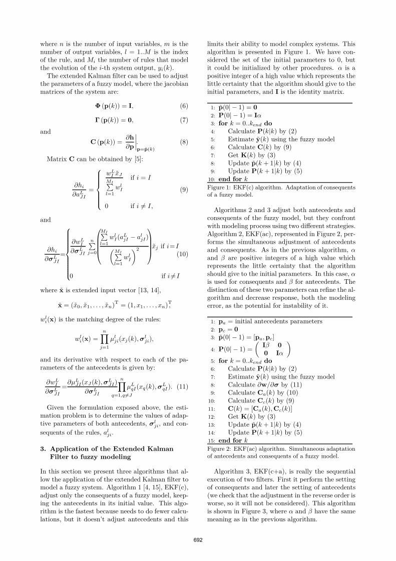
In this section we present three algorithms that al-low the application of the extended Kalman filter tomodel a fuzzy system. Algorithm 1 [4, 15], EKF(c),adjust only the consequents of a fuzzy model, keep-ing the antecedents in its initial value. This algo-rithm is the fastest because needs to do fewer calcu-lations, but it doesn’t adjust antecedents and this

limits their ability to model complex systems. Thisalgorithm is presented in Figure 1. We have con-sidered the set of the initial parameters to 0, butit could be initialized by other procedures. α is apositive integer of a high value which represents thelittle certainty that the algorithm should give to theinitial parameters, and I is the identity matrix.

1: p(0| − 1) = 0

2: P(0| − 1) = Iα3: for k = 0..kend do

4: Calculate P(k|k) by (2)5: Estimate y(k) using the fuzzy model6: Calculate C(k) by (9)7: Get K(k) by (3)8: Update p(k + 1|k) by (4)9: Update P(k + 1|k) by (5)

10: end for kFigure 1: EKF(c) algorithm. Adaptation of consequentsof a fuzzy model.

Algorithms 2 and 3 adjust both antecedents andconsequents of the fuzzy model, but they confrontwith modeling process using two different strategies.Algorithm 2, EKF(ac), represented in Figure 2, per-forms the simultaneous adjustment of antecedentsand consequents. As in the previous algorithm, αand β are positive integers of a high value whichrepresents the little certainty that the algorithmshould give to the initial parameters. In this case, αis used for consequents and β for antecedents. Thedistinction of these two parameters can refine the al-gorithm and decrease response, both the modelingerror, as the potential for instability of it.

1: pa = initial antecedents parameters2: pc = 0

3: p(0| − 1) = [pa, pc]

4: P(0| − 1) =

(

Iβ 0

0 Iα

)

5: for k = 0..kend do

6: Calculate P(k|k) by (2)7: Estimate y(k) using the fuzzy model8: Calculate ∂w/∂σ by (11)9: Calculate Ca(k) by (10)

10: Calculate Cc(k) by (9)11: C(k) = [Ca(k), Cc(k)]12: Get K(k) by (3)13: Update p(k + 1|k) by (4)14: Update P(k + 1|k) by (5)15: end for kFigure 2: EKF(ac) algorithm. Simultaneous adaptationof antecedents and consequents of a fuzzy model.

Algorithm 3, EKF(c+a), is really the sequentialexecution of two filters. First it perform the settingof consequents and later the setting of antecedents(we check that the adjustment in the reverse order isworse, so it will not be considered). This algorithmis shown in Figure 3, where α and β have the samemeaning as in the previous algorithm.

692

1: pc = 0

2: pa = initial antecedents parameters3: Pc(0| − 1) = Iα4: Pa(0| − 1) = Iβ5: for k = 0..kend do

6: Calculate Pc(k|k) by (2)7: Estimate y(k) using the fuzzy model8: Calculate Cc(k) by (9)9: Get Kc(k) by (3)

10: Update pc(k + 1|k) by (4)11: Update Pc(k + 1|k) by (5)12: · · · · · · · · · · · · · · · · · · · · · · · · · · · · · · · · · · · · · · · · · ·13: Calculate Pa(k|k) by (2)14: Estimate y(k) using the fuzzy model15: Calculate ∂w/∂σ by (11)16: Calculate Ca(k) by (10)17: Get Ka(k) by (3)18: Update pa(k + 1|k) by (4)19: Update Pa(k + 1|k) by (5)20: end for kFigure 3: EKF(c+a) algorithm. Separate adaptation ofantecedents and consequents of a fuzzy model.

4. Examples

To demonstrate the practical application of the ex-tended Kalman filter to fuzzy modeling, several ex-amples will be shown. For each case we run thethree algorithms presented in the previous sectionto evaluate their performance: EKF(c), EKF(ac)and EKF(c+a). These examples represent a widerange of possibilities: static and dynamic systemsnonlinear, with only one type of membership func-tion and with mixed functions. Example 3 makes acomparison with a recently published method [17],in order to assess the goodness of the proposed al-gorithms.

4.1. Example 1

Let be the system:

y(x) = e−0.03x sin(0.07x) with x ∈ [−150, 150],

affected by a white noise of covariance Re = 0.5. Weare going to model this system with two differentconfigurations. In the first case, we will use an ini-tial model consisting only of Gaussian membershipfunctions uniformly distributed. In the second case,we will start with a more complex initial model,which consists of several membership functions ofdifferent types, mixed. In order to verify the per-formance of algorithms, we will use the same noisein all cases. The initial covariance matrix for each ofthe algorithms will be initialized with the value thatobtain best performance in each case, i.e., α = 102

for EKF(c) algorithm, α = 103 and β = 10−2 forEKF(ac) algorithm, and α = 1010 and β = 104 forEKF(c+a).

4.1.1. Case I - Gaussian membership functions

Starting from an initial model whose antecedentsare Gaussian membership functions uniformlydistributed, and with all consequents set tozero, we have executed the 3 adjustment algo-rithms. EKF(ac) algorithm has modified an-tecedents slightly, but antecedents resulting fromEKF(c+a) algorithm are shown in Figure 4.

x1(t)

µ(x

)

−150 −100 −50 0 50 100 1500

0.1

0.2

0.3

0.4

0.5

0.6

0.7

0.8

0.9

1

Figure 4: Membership functions resulting from theEKF(c+a) algorithm.

As shown in Figures 5 and 6, algorithm EKF(c)obtains a good model, but their in-line response isnot very good, while algorithm EKF(ac) obtains abetter performance during in-line modeling, but thefinal model obtained is worse than the rest. Thebest result both for in-line modeling and for the fi-nal model validation, is EKF(c+a) algorithm, whichgets a much smaller error in both cases.

The mean final error of EKF(c) algorithm is4.50899, it raises to 6.41349 for EKF(ac) algorithmand drops to 2.21189 for EKF(c+a) algorithm.

Iteration

Err

or

EKF(c)EKF(ac)EKF(c+a)

0 50 100 150 200 250 3000

10

20

30

40

50

60

70

80

Figure 5: Modeling errors during execution.

The fuzzy model obtained by EKF(c+a) is:

693

Iteration

Err

or


0 50 100 150 200 250 3000

5

10

15

20

25

Figure 6: Errors of final models.

R(1,1): IF x is GAUSSMF(-139.773; 35.180)THEN y = −535.075 − 3.977x

R(2,1): IF x is GAUSSMF(-57.928; 55.290)THEN y = −36.671 − 0.746x

R(3,1): IF x is GAUSSMF(46.857; 59.213)THEN y = 9.172 − 0.072x

R(4,1): IF x is GAUSSMF(-21.750; 35.923)THEN y = 13.973 − 0.492x

The response, both in-line models as the finalmodels, can be seen in Figures 7 and 8 respectively.

Iteration

y(t

)

y

yEKF (c)

yEKF (ac)

yEKF (c+a)

0 50 100 150 200 250 300−60

−40

−20

0

20

40

60

80

Figure 7: Run-time response of the models.

Iteration

y(t

)

y

yEKF (c)

yEKF (ac)

yEKF (c+a)

0 50 100 150 200 250 300−40

−20

0

20

40

60

80

Figure 8: Response from the final models.

4.1.2. Case II - Membership functions of differenttype, mixed

In this case the antecedents of the initial model con-sist of a S function, a Z function, a trapezoidal func-tion and a bell function, distributed as shown inFigure 9, and all the consequents initialized to zero.

µ(x

)

x1(t)

−150 −100 −50 0 50 100 1500

0.2

0.4

0.6

0.8

1

Figure 9: Initial membership functions.

As shown graphically in Figures from 10 to 13,the best results for both in-line and final model,again correspond to algorithm EKF(c+a).

Iteration

Err

or


0 50 100 150 200 250 3000

10

20

30

40

50

60

70

80

Figure 10: Modeling run-time errors.

Iteration

Err

or


0 50 100 150 200 250 3000

10

20

30

40


The mean final error of EKF(c) algorithm is5.9141, worse compared to the previous case.

694

Iteration

y(t

)

y

yEKF (c)

yEKF (ac)

yEKF (c+a)

0 50 100 150 200 250 300−40

−20

0

20

40

60

80


Iteration

y(t

)

y

yEKF (c)

yEKF (ac)

yEKF (c+a)

0 50 100 150 200 250 300−40

−20

0

20

40

60

80


EKF(ac) algorithm obtain a slightly worse modelin this case, with an error of 6.4323, while the meanfinal error of the EKF(c+a) algorithm remains thebest, with an mean error of 2.67202.

Antecedents resulting from EKF(c+a) algo-rithm are shown in Figure 14, and the finalfuzzy model obtained by this algorithm is:

R(1,1): IF x is ZMF(-147.53; -85.03)THEN y = −404.844 − 3.084x

R(2,1): IF x is TRAPMF(-135.01; -12.63; -1.53; 29.62)THEN y = −1.733 − 0.114x

R(3,1): IF x is GBELLMF(50.01;2.72;96.02)THEN y = 3.190 − 0.060x

R(4,1): IF x is SMF(50.70;104.76)THEN y = 2.665 + 0.005x

µ(x

)

x1(t)

−150 −100 −50 0 50 100 1500

0.2

0.4

0.6

0.8

1

Figure 14: Membership functions resulting from theEKF(c+a) algorithm.

4.2. Example 2

−

+

u(t)

R

LiL(t)

C

iC(t)

+vC(t)

−

+vR(t)

−

iR(t)

Figure 15: Tunnel diode circuit.

Given the tunnel-diode circuit shown in the Fig-ure 15 [16], where R = 1.5KΩ, C = 2pF andL = 5µH, and whose dynamics can be representedby:

x1(t) =x2(t) − h(x1(t))

C

x2(t) =u(t) − x1(t) − Rx2(t)

L,

where x1(t) = vC(t), x2(t) = iL(t), h(v) is thevR–iR charasteristic of the tunnel-diode, and u(t)is shown in the Figure 16. We assume that the sys-tem is affected by a white noise of covariance:

Re =

(

0.001 00 0.01

)

.

Time(s)

u(t

)

0 50 100 150 200−2

−1

0

1

2

3

Figure 16: Input voltage applied to the circuit u(t).

The initial covariance matrix is set again in or-der to get the best performance, i.e., α = 1010

for EKF(c) algorithm, α = 102 and β = 10−2 forEKF(ac) algorithm, and α = 1010 and β = 104 forEKF(c+a).

After making 100 runs for each of the algorithmsthe results are shown in Table 1. The graphicalrepresentation of mean errors in each of the runscan be seen in Figures 17 and 18.

EKF(c) EKF(ac) EKF(c+a)Mean Time (ms) 0.67781 0.68085 1.20500

In-line Error of x1 × 10−3 0.83199 0.83599 0.78549In-line Error of x2 × 10−3 7.84798 7.83592 7.65570Final Error of x1 × 10−3 0.80531 0.80612 0.80523Final Error of x2 × 10−3 7.73933 7.73932 7.73933

Table 1: Mean values for 100 runs.

695

Iteration

of

x1

Mean Final Error ...

x1(k)EF K(c)

x1(k)EF K(ac)

x1(k)EF K(c+a)

Iteration

of

x2

0 10 20 30 40 50 60 70 80 90 100

0 10 20 30 40 50 60 70 80 90 100

7.5

8

8.5

9

0.5

1

1.5

2

2.5

Figure 17: Modeling run-time errors.

Iteration

of

x1(k

)

Mean Final Error ...

x1(k)EF K(c)x1(k)EF K(ac)x1(k)EF K(c+a)

Iteration

of

x2(k

)

0 10 20 30 40 50 60 70 80 90 100

0 10 20 30 40 50 60 70 80 90 100

7.5

8

8.5

0

2

4

6

8


4.3. Example 3

We have taken a practical example from [17] in orderto compare these methods with a recent one that isknown has a good performance.

Be the nonlinear system:

f(x, y) = 5x2 + 3xy − y2, with x, y ∈ [−4, 4],

affected by a white noise of covariance Re = 3.The initial model consists of Gaussian member-

ship functions uniformly distributed, and the initialcovariance matrix is initialized with the value giv-ing the best performance in this case, i.e., α = 104

for EKF(c) algorithm, α = 102 and β = 10−2 forEKF(ac) algorithm, and α = 105 and β = 10−2 forEKF(c+a). After run 100 times for each of the algo-rithms, the modeling errors are shown in Figures 19and 20, the mean of this values are shown in theTable 2, and the time taken for each run is shownin Figure 21.

EKF(c) EKF(ac) EKF(c+a)Mean Time (ms) 0.17369 0.72062 0.52163

In-line Error 15.70668 8.04251 0.16824Final Error 1.630987 2.03821 1.62997

Table 2: Mean values for 100 runs.

The modeling error of this system obtained in [17]is 0.6086 ± 0.0437. If we compare this result with

Iteration

Mea

nIn

-lin

eE

rror


0 10 20 30 40 50 60 70 80 90 1000

2

4

6

8

10

12

14

16

18

20

22

Figure 19: Run-time modeling mean errors.

Iteration

Mea

nF

inal

Err

or


0 20 40 60 80 100

1.4

1.6

1.8

2

2.2

Figure 20: Modeling mean errors of final models.

Iteration

Mea

nex

ecuti

on

tim

e(s

)


0 10 20 30 40 50 60 70 80 90 1000.1

0.2

0.3

0.4

0.5

0.6

0.7

0.8

0.9

Figure 21: Mean running time.

696

the final mean error obtained in EKF(c+a), 1.62997(see Table 2), we can see the first is slightly better,but note that EKF(c+a) is an in-line algorithm, andits performance in run-time is really good.

With the idea of showing the response of the dif-ferent models obtained has been extracted one ofthe simulations, obtaining the results shown in Fig-ures 22 and 23.

Iteration

f(x

,y)

f(x, y)f(x, y)EKF (c)

f(x, y)EKF (ac)f(x, y)EKF (c+a)

0 10 20 30 40 50 60 70 80 90−150

−100

−50

0

50

100

150


Iteration

f(x

,y)

f(x, y)f(x, y)EKF (c)f(x, y)EKF (ac)f(x, y)EKF (c+a)

0 10 20 30 40 50 60 70 80 90−40

−20

0

20

40

60

80

100

120


5. Conclusions

Two new algorithms based on extended Kalman fil-ter for parametric adaptation of a fuzzy system com-pletely general, i.e., without restrictions on the sizeof the input or output vectors, or the type or distri-bution of membership functions used in the defini-tion of fuzzy sets of the model has been presentedin this paper.

In order to show the generality of the method-ology, several possible alternatives for fit both an-tecedents and consequents of the fuzzy model havebeen presented, and we have obtained several com-paratives of accuracy and efficiency performed onthree examples of nonlinear systems. In view of theresults, it seems evident that the fitting algorithm in

two stages obtains better results both in the evolu-tion of the instantaneous error while running in-linefilter, as in the final models obtained. In addition,with respect to runtime, the EKF(c+a) algorithmhas proven to be faster in most cases.

Tests have shown that these algorithms occasion-ally may diverge, especially the EKF(ac) algorithm,preventing a good in-line behavior. It has also beenobserved in all cases a great dependence on the val-ues assigned to parameters α and β, which recom-mends a previous study of systems to model.

In future works we aim to improve the overallresponse of the algorithms through an in-line studyof the evolution of the modeling process, so as toobtain a more robust performance of these filters.In addition, with respect to the initialization of thecovariance matrices, authors are working on severalalternatives to limit the current dependence of theparameters α and β.

Acknowledgment

The present work is a contribution of the DPI2010-17123 project, funded by the Spanish Ministry forEducation and Science and by the European Re-gional Development Union.

References

[1] Wang Liang and Yen John. Extracting fuzzyrules for system modeling using a hybrid of ge-netic algorithms and Kalman filter. Fuzzy Setsand Systems, 101(3):353–362, February 1999.

[2] Tao Jiang and Yao Tang Li. Generalizeddefuzzification strategies and their parameterlearning procedures. IEEE Transactions onFuzzy Systems, 4(1):64–71, August 1996.

[3] Pramath Ramaswamy, Martin Riese,Robert M. Edwards, and Kwang YoulLee. Two approaches for automating thetuning process of fuzzy logic controllers.In 32nd IEEE Conference on Decision andControl. Part 2 (of 4), San Antonio, TX, USA,December 1993.

[4] Dan J. Simon. Training fuzzy systems withthe extended Kalman filter. Fuzzy Sets andSystems, 132(2):189–199, 2002.

[5] Antonio Javier Barragán Piña, José ManuelAndújar Márquez, Mariano Aznar Torres, andAgustín Jiménez Avello. Methodology foradapting the parameters of a fuzzy system us-ing the extended Kalman filter. In 7th confer-ence of the European Society for Fuzzy Logicand Technology, EUSFLAT (LFA-2011), Aix-les-Bains, France, July 2011.

[6] Agustín Jiménez, Basil M. Al-Hadithi, and Fer-nando Matía. An optimal T-S model for theestimation and identification of nonlinear func-tions. WSEAS Trans. Sys. Ctrl., 3(10):897–906, January 2008.

697

[7] Peter S. Maybeck. Stochastic models, estima-tion, and control, volume 141 of Mathematicsin Science and Engineering. Academyc Press,1979.

[8] Mohinder S. Grewal and Angus P. Andrews.Kalman Filtering: Theory and Practice UsingMATLAB. John Wiley & Sons, Inc., 2nd edi-tion, 2001.

[9] Robert Babuška. Fuzzy modeling – a con-trol engineering perspective. In Proceedings ofFUZZ-IEEE/IFES’95, volume 4, pages 1897–1902, Yokohama, Japan, March 1995.

[10] Robert Babuška, Magne Setnes, Uzay Kay-mak, and Hans R. van Nauta Lemke. Rule basesimplification with similarity measures. In Pro-ceedings of the 5th IEEE International Confer-ence on Fuzzy Systems, volume 3, pages 1642–1647, New Orleans, LA, September 1996.

[11] Hung T. Nguyen, Michio Sugeno, Richard M.Tong, and Ronald R. Yager. Theoretical aspectsof fuzzy control. John Wiley Sons, 1995.

[12] T. Takagi and M. Sugeno. Fuzzy identificationof systems and its applications to modeling andcontrol. IEEE Transactions on Systems, Man,and Cybernetics, 15(1):116–132, 1985.

[13] José Manuel Andújar and Antonio Javier Bar-ragán. A methodology to design stable non-linear fuzzy control systems. Fuzzy Sets andSystems, 154(2):157–181, September 2005.

[14] José Manuel Andújar, Antonio Javier Bar-ragán, and Manuel Emilio Gegúndez. A gen-eral and formal methodology for designing sta-ble nonlinear fuzzy control systems. IEEETransactions on Fuzzy Systems, 17(5):1081–1091, October 2009.

[15] Fernando Matía, Agustín Jiménez, Basil M. Al-Hadithi, Diego Rodríguez-Losada, and RamónGalán. The fuzzy Kalman filter: State estima-tion using possibilistic techniques. Fuzzy Setsand Systems, 157(16):2145–2170, August 2006.

[16] H. K. Khalil. Nonlinear systems. Prentice-Hall,NJ, 2000.

[17] Seok Beom Roh, Tae Chon Ahn, and WitoldPedrycz. The refinement of models with theaid of the fuzzy k-nearest neighbors approach.IEEE Transactions on Instrumentation andMeasurement, 59(3):604–615, March 2010.

698

application of the extended kalman filter to fuzzy - atlantis press

Documents