fuzzy logic applied to adaptive kalman filtering

University of Nebraska - Lincoln University of Nebraska - Lincoln

DigitalCommons@University of Nebraska - Lincoln DigitalCommons@University of Nebraska - Lincoln

Theses, Dissertations, and Student Research from Electrical & Computer Engineering

Electrical & Computer Engineering, Department of

December 1992

Fuzzy Logic Applied to Adaptive Kalman Filtering Fuzzy Logic Applied to Adaptive Kalman Filtering

Marlys Rae Remus University of Nebraska - Lincoln

Follow this and additional works at: https://digitalcommons.unl.edu/elecengtheses

Part of the Electrical and Computer Engineering Commons

Remus, Marlys Rae, "Fuzzy Logic Applied to Adaptive Kalman Filtering" (1992). Theses, Dissertations, and Student Research from Electrical & Computer Engineering. 3. https://digitalcommons.unl.edu/elecengtheses/3

This Article is brought to you for free and open access by the Electrical & Computer Engineering, Department of at DigitalCommons@University of Nebraska - Lincoln. It has been accepted for inclusion in Theses, Dissertations, and Student Research from Electrical & Computer Engineering by an authorized administrator of DigitalCommons@University of Nebraska - Lincoln.

https://digitalcommons.unl.edu/

https://digitalcommons.unl.edu/elecengtheses

https://digitalcommons.unl.edu/elecengtheses

https://digitalcommons.unl.edu/electricalengineering

https://digitalcommons.unl.edu/electricalengineering

https://digitalcommons.unl.edu/elecengtheses?utm_source=digitalcommons.unl.edu%2Felecengtheses%2F3&utm_medium=PDF&utm_campaign=PDFCoverPages

http://network.bepress.com/hgg/discipline/266?utm_source=digitalcommons.unl.edu%2Felecengtheses%2F3&utm_medium=PDF&utm_campaign=PDFCoverPages

https://digitalcommons.unl.edu/elecengtheses/3?utm_source=digitalcommons.unl.edu%2Felecengtheses%2F3&utm_medium=PDF&utm_campaign=PDFCoverPages

FUZZY LOGIC APPLIED TOADAPTIVE KALMAN FILTERING

by

Marlys Rae Remus

A THESIS

Presented to the Faculty of

The Graduate College at the University of Nebraska

In Partial Fulfillment of Requirements

For the Degree of Master of Science

Major: Electrical Engineering

Under the Supervision of Professor A. John Boye

Lincoln, Nebraska

December, 1992

FUZZY LOGIC APPLIED TO

ADAPTIVE KALMAN FILTERING

Marlys Rae Remus, M.S.

University of Nebraska, 1992

Adviser: A. John Boye

The Kalman filter provides an effective means of

estimating the state of a system from noisy measurements

given that the system parameters are completely specified.

The innovations sequence for a properly specified Kalman

filter will be a zero-mean white noise process. However,

when the system parameters change with time the Kalman

filter will need to be adapted to compensate for the

changes. Traditionally this has been accomplished by using

nonlinear filtering, parallel Kalman filtering and

covariance matching techniques. These methods have produced

good results at the expense of large amounts of

computational time. Necessary changes in the system

parameters become obvious when the innovations sequence is

examined.

Fuzzy logic is an attempt to program human experience

into control systems by using a simple set of linguistic

rules. In recent years, the use of fuzzy logic has been

applied to several types of control systems.

In this thesis, an adaptive algorithm which employs

fuzzy logic rules is used to adapt the Kalman filter to

accommodate changes in the system parameters. The adaptive

algorithm examines the innovations sequence and makes the

appropriate changes in the Kalman filter model. To

illustrate the effectiveness of this approach, a target

tracking system which employs an adaptive Kalman filter to

estimate target position is designed and tested.

TABLE OF CONTENTS

CHAPTER TITLE PAGE

I. Introduction 1

II. Fuzzy Set Theory 3

III. Fuzzy Logic Applied to Control 17Systems

IV. The Kalman Filter 22

V. Fuzzy Logic Adaptive Kalman 32Filter Applied to a TargetTracking System

V.1 Multiple Target Tracking 32System

V.2 Target Simulation 36

V.3 Method 1 38

V.4 Method 2 44

V.5 Method 3 50

V.6 Method 4 53

V.7 Computational Burden 59

VI. Conclusion 61

References 63

I. Introduction

In recent years, fuzzy logic, which was originally

designed to imitate the human decision making process, has

been a popular topic of control systems research. It has

proven to be effective with difficult to control processes

and systems where the control objectives are specified

qualitatively. Researchers have found that control systems

which employ fuzzy algorithms are robust and more fault

tolerant.


estimating the state of a system from noisy measurements

when the system is well defined and the system covariances

are known. However, in real world problems it is frequently

impossible to completely define the system. In this case,

it is necessary to adapt the Kalman filter model. Several

different approaches have been successful in adapting the

Kalman filter model at the expense of an increase in

computational burden. An adaptive algorithm which employs

fuzzy logic to adapt the Kalman filter model is proposed in

this paper. The algorithm examines the innovations sequence

and makes the appropriate changes in the Kalman filter

model.

A discussion of fuzzy set theory and its application to

control systems is presented, followed by an introduction to

the Kalman filter and a discussion of the various adaptive

techniques currently in use. The properties of the

2

innovations sequence of a properly specified Kalman filter

are discussed. These properties will be used to formulate

the fuzzy control rules to be used in the fuzzy logic

algorithm.

To illustrate the effectiveness of this approach, a

fuzzy logic adaptive Kalman filter algorithm is designed and

implemented in a target tracking system. The results

indicate that this is a valid approach to adaptive Kalman

filtering.

3II. Fuzzy Set Theory

A classical set is defined as a collection of objects

called elements. A classical set can be described in a

number of ways. One way is to simply list the elements of

the set. For example, the set of primary colors would be

described by the following list, {red, blue, yellow}.

Another and perhaps more useful method is to describe the

set analytically. For example, let the set A denote the set

of all real numbers less than 5.0. The set A can then be

described in the following set notation, A = {xeXlx<5.0}. A

third method employs a characteristic function, F(x). Where

F(x)=l indicates membership of the element x in the set A

and F(x)=O indicates non-membership of the element x in the

set A. The characteristic function for the set of all real

numbers less than 5.0 is shown in Figure 2.1.

2,----------------..,

1.8

I.&

1.4

1.2-

D.S

o.&-

0.4

0.2-

o 2 3 4 S 6 1 8 9 10REAL NlJABERS

Figure 2.1 Characteristic function for a classical setof real numbers less than 5.0.

All of these methods have one thing in common, either an

element belongs to the set or it does not. Therefore,

4

classical set theory is dichotomous in nature. On the other

hand, fuzzy sets have the advantage of allowing varying

degrees of membership.

A fuzzy set as defined by Zimmerman [1] is a set of

ordered pairs, (x,p(x)) and may be described using set

notation. For example, the set A can be described as

follows: A={(x,p(x))lxeX}; where x is an element in the set

x, p is the membership function which maps each element x in

X into the membership space, and p(x) is the grade of

membership of the element x in the fuzzy set A. For

example, let A be a fuzzy set of temperatures around 75

degrees, X is a set of all possible temperatures generically

denoted by x and p(x) is defined as shown in Figure 2.2a.

2

.8

.&

.4

.2-

1

8

6

4

2

050 55 60 65 70 7S 60 8S 90 95 100

TEMPERATURE

0.

~ 1

§ 1

~u. 1

~i!la::~ 0.

~ 0.

() 0.

o.j-..-.--.........<;----...-,.---..---;:.-....- ~50 55 60 65 70 7S 80 8S 90 95 100

TEMPERATURE

0.4

0.2

1.8

2,.-----------------,

Figure 2.2a Membership function for thefuzzy set of temperatures around 75degrees.

Figure 2.2b Characteristic function for theclassical set of "temperatures around 75

degrees".

A temperature of 68 degrees has a membership of 0.50 in the

fuzzy set of temperatures around 75 degrees compared to a

membership of 1.0 in the classical characteristic function

5

shown in Figure 2.2b. Therefore, a fuzzy set is very well

suited to handling the situation where the set is not

clearly defined. The key to defining any fuzzy set is

selecting a linguistic variable that describes the set.

Simply stated, a linguistic variable is a variable

whose values are words instead of numbers. Zadeh [2]

defined a linguistic variable as a quintuple,

(X,T(X),U,G,M). Where X is the name of the variable, T(X)

is the "term set" of the possible values which the

linguistic variable can take on, U is the universe of

discourse, G is a syntactic rule which generates the terms

in the term set and M is the semantic rule which associates

a meaning to each value in the term set and can be viewed as

a fuzzy subset of the variable X. For example, the

linguistic variable AGE would have a universe of discourse

which includes all positive whole numbers and one possible

term set would be {young, middle aged, old}.

The final step in defining a linguistic variable is to

develop membership functions each fuzzy subset. The fuzzy

subsets are described by the meanings associated with each

element in the term set. These functions are used to map

each nonfuzzy value of the variable into the fuzzy subsets.

The grade of membership of an element x in a particular

fuzzy set A can be viewed as a comparison of x to the ideal

value for the set A [1]. This results in a perceived

6

distance, d(x). The membership function for the fuzzy set A

would then be defined as follows.

1jJ.(x) = l+d(x) (2.1 )

Where d(x) is a function of the element x and would

determine the shape of the membership function. Notice that

a very small distance would result in a grade of membership

very close to 1 and a large distance would result in a grade

of membership very close to O. There is very little

justification for the general shape of a membership

function. For the linguistic variable AGE defined above,

the ideal values for the subsets young, middle aged and old

could be defined as shown in Figure 2.3a. Notice that these

are nonfuzzy sets and that not all ages fall into a

category. For instance, the age 30 is neither young nor

middle aged but some where in between. Figure 2.3b shows

the membership functions for the fuzzy sets young, middle

aged and old.

0.4

Ol-l--__-""'~__-_"-""'-....__.....Io 10 20 :lO 40 50 eo 70 80 90 100

AGE IN YEARS

Q.2

211.8

1.6

~ 1.4w!!1 1.2

~ 1+----..isw o.ll

~ 0.8

"

I

~iJ nJ

I I

2

oo 10 20 ~ 40 50 eo 70 80 90 100I'.GEINYEAAS

'" 1.8

5G 1.6

~ lA...~ 1.2

if 1w....~ 0.8

~ 0.6()

~ 0.4

QQ.2

Figure 2.3a. Characteristic functions theideal subsets young, middle agedand old.

Figure 2.3b. Membership functions for thefuzzy subsets young. middle aged

and old.

7

Similar to classical set theory, it is possible to

perform operations on fuzzy sets. The three most commonly

used set operations are the intersection of two sets, the

union of two sets and the complement of a set. In classical

set theory, the intersection of two sets, A and B, is

defined to be the set of elements that are common to both

set A and B. In fuzzy set theory, the intersection of two

sets A and B is defined to be the minimum grade of

membership of sets A and B [1,3]. For example, let set A be

the intersection of the fuzzy sets young and middle aged

shown in Figure 2.3b.

llA (x) = min (llYOUNG (x) ,llMIDDLE AGED (x) )

The membership function for the set A is shown in Figure

2.4.

111

O"!",o---:"1":"'0--:':20:-'-30~-4""0 --:':60~6""0~7~O --:':80-90""--1100AGE IN YEARS

Figure 2.4. Membership function for theintersection of the two fuzzy subsets youngand middle aged.

The union of two sets A and B is defined in classical

set theory to be the set of all elements in both sets A and

B. In fuzzy set theory, the union is defined to be maximum

grade of membership of the element in sets A and B [1,3].

For example let B be the fuzzy set defined as the union of

the fuzzy sets middle aged and old shown in Figure 2.3b.

11B (x) = max (llMIDDLE AGED (x) , 1l0LD (x) )

The membership function for set B is shown in Figure 2.5.2,--------------,

1.8

Figure 2.5. Membership function for theunion of the two fuzzy subsets middle aged and old.

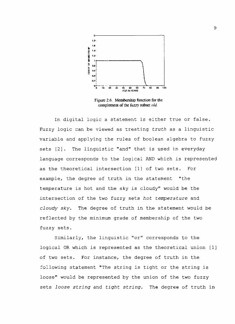
The complement of a classical set, A, is defined as a

set of all elements not included in set A. In fuzzy set

theory the complement is defined by the following equation

[1,3] .llCOMPLEMENT (x) = 1.0 - 11 (x)

For example let C be the complement of the fuzzy set old

shown in Figure 2.3b.

llC(x) = 1.0 - lloLD(x)

The membership function for the set C is shown in Figure

2.6.

8

9

2,--------------,1.8j

i! 1.~<ii 1.4

5::0 1:!~ 1+----------,.o 0.8

i ::~o.2~

o,+-'-~__,___~-~_~~r-"-....--~o 10 20 30 40 SO 60 70 80 00 100

AGE IN YEARS

Figure 2.6. Membership function for thecomplement of the fuzzy subset old.

In digital logic a statement is either true or false.

Fuzzy logic can be viewed as treating truth as a linguistic

variable and applying the rules of boolean algebra to fuzzy

sets [2]. The linguistic "and" that is used in everyday

language corresponds to the logical AND which is represented

as the theoretical intersection [1] of two sets. For

example, the degree of truth in the statement "the

temperature is hot and the sky is cloudy" would be the

intersection of the two fuzzy sets hot temperature and

cloudy sky. The degree of truth in the statement would be

reflected by the minimum grade of membership of the two

fuzzy sets.

Similarly, the linguistic "or" corresponds to the

logical OR which is represented as the theoretical union [1]

of two sets. For instance, the degree of truth in the

following statement "The string is tight or the string is

loose" would be represented by the union of the two fuzzy

sets loose string and tight string. The degree of truth in

10

the statement would be reflected by maximum grade of

membership of the two fuzzy subsets.

The complement of a fuzzy set corresponds to the

linguistic "not" [1]. For example, the degree of truth in

the following statement "The temperature is not hot" would

be represented by the complement of the fuzzy set hot

temperature. By using these three operators, it is very

easy to construct a set of control rules using common

everyday language. An example of a typical control rule

would be "If the error is POSITIVE LARGE AND the change ~n

error is NEGATIVE, then the change in control input is SMALL".

A collection of this type of control rule is said to be a

fuzzy control algorithm [4].

As shown in Figure 2.7, there are four principal

components in a fuzzy logic control algorithm [5]. The

fuzzification interface maps the real inputs to fuzzy sets.

This is usually accomplished using membership functions.

The knowledge base is comprised of two components [5],

the rule base and the data base. The rule base

characterizes the control goals and control policy by means

of a set of linguistic control rules. The data base

provides the necessary membership functions used in the

linguistic control rules and fuzzy data manipulation. The

decision making logic component employs rules of inference

in fuzzy logic to determine a fuzzy control input. This is

11

accomplished by using boolean algebra to determine the

degree of fulfillment of each rule.

KNOWLEDGE BHE

.. P ....PUZZUIC:R.TION DEPUnIPIC:R.TION

INTEU:R.CE :Ul'fEU:lCE

~ .. ~ ..... •puzzr puzzr.... DECISION MJlKING

r LOGIC

SYSTEM OUTPUT CONTEOL :R.CTION

SYSTEM ....,.

Figure 2.7 Block diagram of a fuzzylogic control system.

Consider the following control rule, the degree of

fulfillment would be the intersection of the fuzzy subset

POSITIVE LARGE for the linguistic variable error and the fuzzy

subset NEGATIVE for the linguistic variable change in error.

If the error is POSITIVE LARGE AND thechange in error is NEGATIVE, then thechange in control input is SMALL.

For example, an error which produces a grade of membership

of O. 75 in the fuzzy subset POSITIVE LARGE and a change in

12

error which produces a grade of membership of 0.25 in the

fuzzy subset NEGATIVE, would have a degree of fulfillment of

0.25 in the fuzzy subset SMALL for the linguistic variable

change in control input.

The defuzzification interface converts the fuzzy

control to a real control action. The defuzzification stage

can be viewed as a mapping of fuzzy control actions defined

over an output universe of discourse into nonfuzzy control

actions. There are currently three defuzzification

strategies commonly in use [5]. The maximum criterion

method of defuzzification produces the control action

associated with the rule which has the highest degree of

fulfillment (DOF).

II (max DOF) (2.2)

The operator, ll, is a defuzzification function which maps

the fuzzy valued control into a real valued control.

The mean of maximum method produces the control action

which represents the mean value of all local control actions

whose membership functions reach the maximum. The nonfuzzy

control action is calculated using the following equation.

k

L W·20 = -.2

k

j=l

(2.3)

13

The nonfuzzy control action required by the jth rule is

denoted as Wj and k is the number of control actions which

reach a maximum.

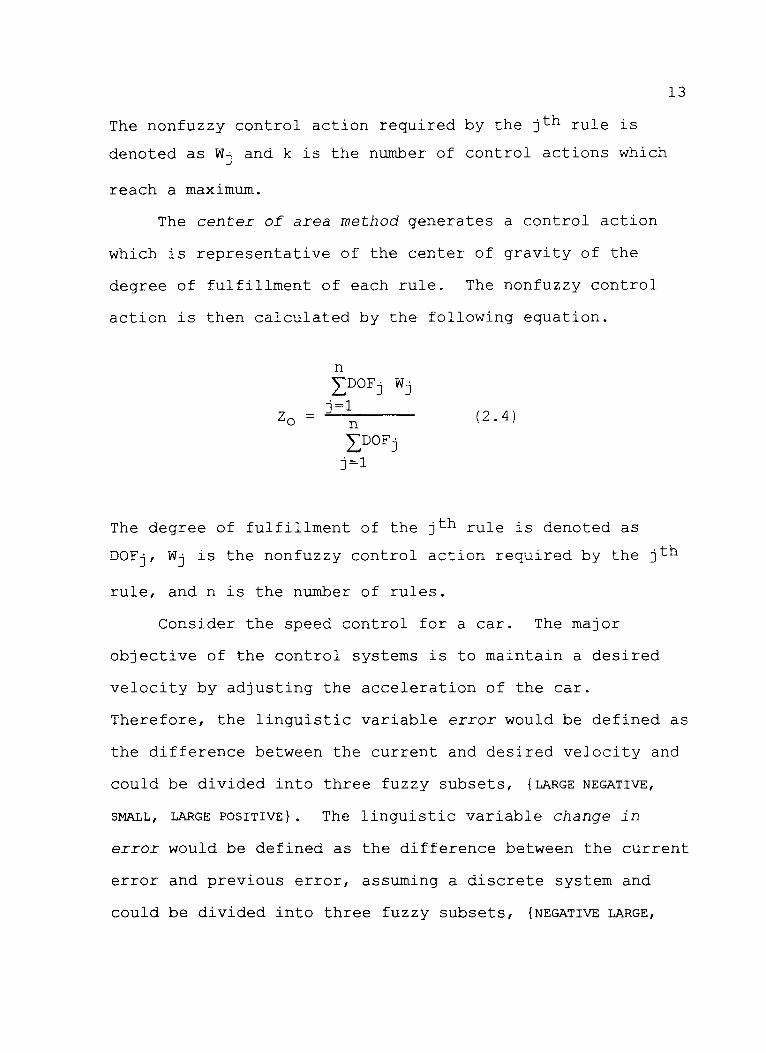
The center of area method generates a control action

which is representative of the center of gravity of the

degree of fulfillment of each rule. The nonfuzzy control

action is then calculated by the following equation.

(2.4)

The degree of fulfillment of the jth rule is denoted as

DOFj, Wj is the nonfuzzy control action required by the jth

rule, and n is the number of rules.

Consider the speed control for a car. The major

objective of the control systems is to maintain a desired

velocity by adjusting the acceleration of the car.

Therefore, the linguistic variable error would be defined as

the difference between the current and desired velocity and

could be divided into three fuzzy subsets, {LARGE NEGATIVE,

SMALL, LARGE POSITIVE}. The linguistic variable change in

error would be defined as the difference between the current

error and previous error, assuming a discrete system and

could be divided into three fuzzy subsets, {NEGATIVE LARGE,

14

SMALL, POSITIVE LARGE} • These fuzzy subsets are defined by the

membership functions given in Figure 2.8.

1.

• •

•

1.4•

,.

' .1.

I :1

''\, · vV' ",,- /V'0.8 " • •

•

",,- ,/ ",,- · V0.6- ---_. ./

)( X·•

/V '" V ",0.2

, //.

• • f"- v. . . .""0/. /. f

11-10-9 -8 -7 ·6 -S -4 -3 ·21 0 1 2 3 4 S 6 7 8 91011ERROR

1...

••

. ' .•

•1.4- , .. .

. '

.•..........

.•

'. · .

••

• , •

1

N V\ I•'..0.8

\ V /\[Xi •• 'X •. '"

",V ... \. . V',,' · ' .

V \/ ·N .0

.'. . •• • •

·11-10-9-87 G&4-3-2-1 0 123" & 6 7 8 91011CHANGE IN ERROR

Figure 2.8 Membership functions for the linguistic variableserror and change in error.

The control rules listed in Table 2.1 could be used to

regulate the acceleration of the car. An input error of

-2.0 ft/sec would have a grade of membership of 0.2 in the

fuzzy subset LARGE NEGATIVE, 0.8 in the fuzzy subset SMALL and

0.0 in the fuzzy subset LARGE POSITIVE. Similarly, a change

in error of 4.0 ft/sec would result in grades of membership

of 0.0, 0.2, and 0.8 for the fuzzy subsets LARGE NEGATIVE,

SMALL, and LARGE POSITIVE, respectively. The degree of

fulfillment of each rule is then found using boolean

algebra. For example, the first rule listed in Table 2.1

has a degree of fulfillment of 0.0 in the nonfuzzy set of

+5.0 ft/sec 2 for the linguistic variable change in

acceleration. The degree of fulfillment for all of the

rules listed in Table 2.1 is given in vector form below.

151. If the error is LARGE NEGATIVE and the change in

error is NEGATIVE LARGE, then the change inacceleration is +5.0 ft/sec 2 .

2. If the error is LARGE NEGATIVE and the change inerror is SMALL, then the change in accelerationis +2.5 ft/sec 2 .

3. If the error is LARGE NEGATIVE and the change inerror is POSITIVE LARGE, then the change inacceleration is 0.0 ft/sec 2 .

4. If the error is SMALL, then the change inacceleration is 0.0 ft/sec 2 .

5. I f the error is LARGE POSITIVE and the change inerror is negative large, then the change inacceleration is 0.Oft/sec2 .

6. If the error is LARGE POSITIVE and the change inerror is SMALL, then the change in accelerationis -2.5 ft/sec 2 .

7. If the error is LARGE POSITIVE and the change inerror is POSITIVE LARGE, then the change inacceleration is -5.0 ft/sec2 .

Table 2.1 Control rules for speed control of a car.

0.00.20.2

DOF 0.80.00.00.0

Since rule four is the only rule that has a maximum

degree of fulfillment, the maximum criterion method and mean

of maximum method result in the same change in acceleration,

16

0.0 ft/sec 2 . Using the center of area method and Equation

2.4 results in an increase in acceleration of 0.42ft/sec2 .

Fuzzy logic control was originally applied to systems

which traditionally were controlled by a human operator.

However, in recent years fuzzy logic control has proven

effective in a variety of different types of systems.

17III. Fuzzy Logic Applied to Control Systems

conventional control techniques have proven to be very

successful in areas where the system and control objectives

are well defined. However, when the structure of the system

is unknown, the parameter variation in the system is

extensive or the constraints are not quantifiable by a

single value, the effectiveness of conventional control

techniques diminish. Fuzzy logic control (FLC), originally

designed to emulate the behavior of a human operator, has

proven to be an effective means of dealing with such

problems. FLC was first applied in the area of difficult to

control tasks which were traditionally performed by a human

operator [6,7]. Later it was applied to control systems

where conventional control techniques were currently in use

[8,9]. This led some researchers to consider that the fuzzy

logic approach should be used in a complementary manner with

conventional control techniques [10, 11] .

Kickert and van Nauta Lemke [6] applied fuzzy logic to

control the temperature of a warm water plant. The aim of

the controller was to maintain a specified steady state

temperature and cold water flow by adjusting the hot water

flow. Earlier investigations showed that this process had

properties which made it difficult to control using

traditional control strategies. These properties included

nonlinearities, asymmetric behavior for heating and cooling

and disturbances due to the ambient temperature. An

18

ordinary PI controller was designed to get a comparative

idea of the controller performance. The fuzzy controller

exhibited a faster rise time and smaller overshoot compared

to the PI controller. The steady state error of both the PI

and fuzzy controllers was small.

Bernard [7] designed and implemented a rule based,

digital closed loop controller that incorporates fuzzy logic

in the control of power in a nuclear reactor. The equations

for reactor dynamics are nonlinear and there are power

dependent feedback effects that must be taken into account.

Additional complications arise from the fact that the

reactivity is not directly measurable and the change in

reactivity is a nonlinear function of rod position. The

fuzzy and analytic controllers were comparable with respect

to accuracy. The fuzzy controller achieved proper control

over a wider range of initial conditions than the analytic

controller, it was less sensitive to high frequency noise

and more tolerant of sensor failure than the analytic

controller. The analytic controller had a more rapid time

response and was easier to maintain than the fuzzy

controller. Bernard concluded that the fuzzy rule based and

analytic approaches both have advantages and disadvantages

and should be used in tandem to create truly robust control

systems.

Rockwell International [8] developed an aircraft model

called the Advanced Technology Wing (ATW) to explore issues

19

related to light weight flexible wing aircraft. The ATW was

designed to use active controls to provide wing shapes that

optimize particular flight performance criterion. The

control system must be designed to cope with the conflicting

objectives of optimizing flight performance and limiting

wing loads to maintain safety. Conventional control

techniques exhibited a large overshoot and a long settling

time and attempted to alleviate wing loads even though the

current loads were well within acceptable limits. A fuzzy

logic based controller was designed to modulate control

surfaces on the wing to achieve adequate flight performance

while ensuring that wing loads are within acceptable bounds.

The fuzzy logic controller provided excellent system

response and highly flexible control behavior that operated

the system close to the constraint limits and sacrificed

maneuver performance only when critically necessary.

Li and Lau [9] investigated the possibility of using

fUzzy algorithms in the control of a servomotor. The task

of the control algorithm is to rotate the shaft of the motor

to a set position without overshoot. The fuzzy control

rules were based on the error and change of error between

the set point and the measured shaft position. A good

control system for a servomotor is characterized by fast

response time and a small steady state error. For purposes

of comparison, a PID and MRAC controllers were also

designed. The fuzzy controller exhibited a smaller settling

20

time than either the PID or MRAC controllers. Both the

fuzzy and MRAC controllers maintained a small steady state

error. The PID controller was sensitive to disturbances,

which caused larger steady state errors. Li and Lau

observed three advantages for using fuzzy algorithms in this

type of control system. The fuzzy controller did not

require a detailed mathematical model to formulate the

algorithms, had more adaptive capabilities, and was able to

operate for a large range of inputs. Even though the fuzzy

controller performed well in this application , the

researchers expressed concerns over the lack of practical

methods for controller calibration and the lack of guidance

on the shape of membership functions and the overlapping of

fuzzy subsets.

Yoshida and Wakabayashi [10] developed a bang-bang

controller for a rigid disk drive which employed a fuzzy

logic algorithm to estimate the switching time and make

corrections for changes in actuator coil resistance due to

temperature changes. Conventional disk drives depend on

closed loop velocity profile control. The deceleration

profile is set somewhat low so as to absorb the scattering

in actuator parameters. The limits on the deceleration

profile constrain the seek time and it is difficult to

exploit the full capabilities of the actuator. The bang

bang controller uses maximum acceleration for acceleration

and deceleration. By using fuzzy logic to estimate the

21

switching time, the average seek time was reduced by 20% to

30% compared to the conventional method. Using fuzzy logic

to correct for actuator force unevenness, enabled a

significant improvement in the scattering of position

deviations.

Jang and Chen [11] developed a fuzzy modeling algorithm

to construct a set of fuzzy linguistic rules to imitate the

behavior of a state feedback controller. To illustrate the

effectiveness of the algorithm it was applied to the

inverted pendulum problem. The fuzzy controller performed

at least as good as the state feedback controller. Even

though the fuzzy control algorithm was rather cumbersome,

the researchers cited two advantages in using the fuzzy

control approach. The fuzzy controller was more robust and

fault tolerant than the state feedback controller. Secondly,

the format of the linguistic rules was more likely to

extract the behavior of the system and to give a better

understanding of the trend of the system when some

parameters vary.

Many control systems applications require accurate

estimates of the system states. These state estimates can

be supplied by a Kalman filter if the system model can be

accurately defined. However, in real world applications the

system may contain unknown or time varying parameters. The

Kalman filter will need to have the capability of

identifying the unknown system parameters.

22IV. The Kalman Filter

The need for accurate state estimates often arises in

control systems applications. The performance of a state

estimator is usually judged by two criterion. First, the

estimator needs to be accurate. Therefore, the mean error

should be as small as possible, ideally zero. The estimator

also needs to provide a precise estimate of the current

state. Therefore, the covariance of the error should be

small. The optimal estimate based on the error variance

criterion is called the minimum variance estimate.


solving the minimum variance estimation problem for a linear

system with noisy measurements linearly related to the

states. A linear discrete system can be described by the

following set of equations.

SYSTEM MODEL

x(k+1) = Ax(k) + Ww(k) (4.1a)

w(k) is a zero mean white process noisewith covariance Rw.

MEASUREMENT MODEL

y(k)= Cx(k) + v(k) (4.1b)

v(k) is a zero mean white process noisewith covariance Rv .

The Kalman filter algorithm can be viewed as a predictor-

corrector algorithm as shown in Figure 4.1 [12].

23

INITIAL CONDITIONS

PREDICTION

INNOVATIONSSEQUENCE

CORRECTION

_-004 MEASUREMENT

Figure 4.1 Block diagram of Kalman filter algorithm.

The derivation of this algorithm is done in many

standard text books and will not be undertaken here. The

Kalman filter algorithm shown in Figure 4.1 and Table 4.1

assumes that the system state transition matrix, measurement

model and the covariances of the plant and measurement noise

are known. This is rarely the case in the real world. A

properly specified Kalman filter will have the properties

given in Table 4.2 [12].

Adaptive filtering is an on line process of trying to

identify unknown system parameters based on the

measurements and innovations sequence as they occur in real

time [13]. The innovations sequence of a properly specified

Kalman filter should be a purely random process. Several

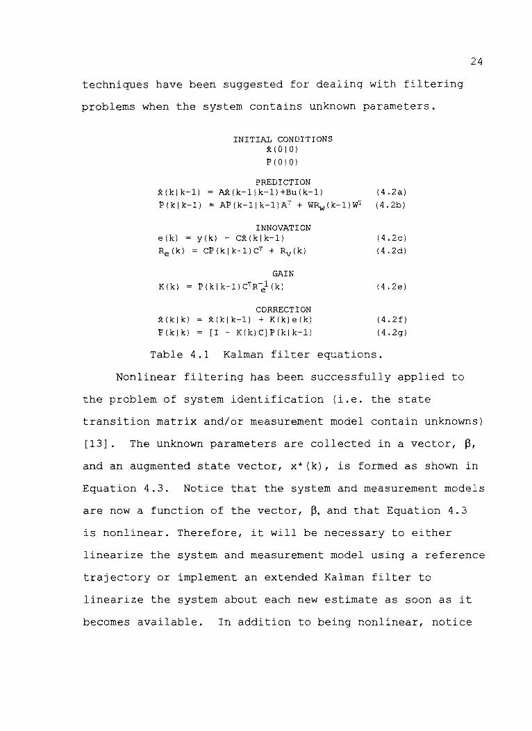
24

techniques have been suggested for dealing with filtering

problems when the system contains unknown parameters.

INITIAL CONDITIONS~ (0 10)

P (0 10)

PREDICTION~(klk-l) ~(k-llk-l)+Bu(k-l)

P(klk-l) = AP(k-llk-l)AT + WRw(k-l)WT

INNOVATIONe(k) = y(k) - C~(klk-l)

Re(k) = CP(klk-l)CT + Rv(k)

(4.2a)

(4.2b)

(4.2c)

(4.2d)

K(k)

~(kl k)

P(klk)

GAIN

P (k Ik-l) CTR-e1 (k)

CORRECTION~(klk-l) + K(k)e(k)

[I - K(k)C]P(klk-l)

(4.2e)

(4.2f)

(4.2g)

Table 4.1 Kalman filter equations.

Nonlinear filtering has been successfully applied to

the problem of system identification (i.e. the state

transition matrix and/or measurement model contain unknowns)

[13]. The unknown parameters are collected in a vector, ~,

and an augmented state vector, x*(k), is formed as shown in

Equation 4.3. Notice that the system and measurement models

are now a function of the vector, ~, and that Equation 4.3

is nonlinear. Therefore, it will be necessary to either

linearize the system and measurement model using a reference

trajectory or implement an extended Kalman filter to

linearize the system about each new estimate as soon as it

becomes available. In addition to being nonlinear, notice

251. Innovations sequence is zero-mean.

2. Innovations sequence is white.

3. Innovations sequence is uncorrelated in time.

4. Innovations sequence lies within the confidenceinterval constructed from Re of the Kalmanfilter algorithm. The innovations sequence willhave a normal distribution. Therefore, lessthan five percent of the innovations will beoutside two estimated standard deviations. Theconfidence interval is then constructed usingthe following equations.

upper limit = 2.0 ~

lower limit = -2.0 ~

5. The actual variance of the innovations sequencewill be reasonably close to the estimatedvariance, Re .

6. Estimation error lies within the confidencelimits constructed from estimated errorcovariance, ~, of the Kalman filter algorithm.The estimation error will have a normaldistribution. Therefore, less than fivepercent of the estimation errors will be outsidetwo estimated standard deviations. Theconfidence limits will be constructed using thefollowing equations.

upper limit = 2.0 ~

lower limit = -2.0 ~

7. The actual error variance is close to theestimated variance .

Table 4.2 Properties of properly specifiedKalman filter [12].

that the order of the system will increase which in turn

leads to a substantial increase in the computational burden.

26

AUGMENTED SYSTEM MODEL

[X (k+1)]

x*(k+1) = B(k+1)

x*(k+1) = [A (B) 0] [X (k) ] [w (k) ]o I B(k) + wB (k) (4.3a)

The parameters w(k) and wB(k) are zero meanwhite process noise with covariances

Rw and RwB respectively.

AUGMENTED MEASUREMENT MODEL

[

X (k)]y(k) = (C(B)O) B(k) + v(k) (4. 3b)

The parameter v(k) is zero mean white processnoise with covariance Rv .

Another technique which yields a pleasing solution form

is conditional mean estimation [13]. This method assumes

that the system and observation models are linear and that

all random processes are Gaussian. The unknown parameters

are represented by a vector, B, and must be selected from a

known finite set, L. The conditional estimate of the state,

x(k), given the measurement set, y(k), can be written as

shown below.

~(k) = f(x(k)P[x(k),y(k)]dx(k))

jt ( k I = JP [Ill y (k) JJ(x (k) P [x ( k) Ill, y (k) ] dx (k I I dll

L

(4.4a)

(4.4b)

27

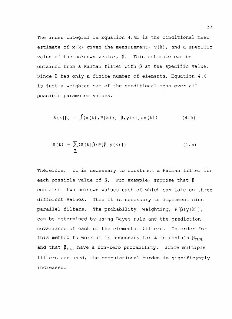
The inner integral in Equation 4.4b is the conditional mean

estimate of x(k) given the measurement, y(k), and a specific

value of the unknown vector,~. This estimate can be

obtained from a Kalman filter with ~ at the specific value.

Since ~ has only a finite number of elements, Equation 4.6

is just a weighted sum of the conditional mean over all

possible parameter values.

~(kl~) = J(x(k) ,P[x(k) I~,y(k) ]dx(k))

~(k) Z>~(kl~)PWly(k)])

~

(4.5)

(4.6)

Therefore, it is necessary to construct a Kalman filter for

each possible value of~. For example, suppose that ~

contains two unknown values each of which can take on three

different values. Then it is necessary to implement nine

parallel filters. The probability weighting, P[~ly(k)],

can be determined by using Bayes rule and the prediction

covariance of each of the elemental filters. In order for

this method to work it is necessary for ~ to contain ~T~E

and that ~TRUE have a non-zero probability. Since multiple

filters are used, the computational burden is significantly

increased.

28

Covariance matching [13] has proven to be effective in

estimating the covariance of both the plant and measurement

noise. This technique simply equates the time average

approximation and the theoretical covariance of the

innovations sequence. The disadvantage of using this

approach is that it completely ignores the fact that the

innovations sequence is supposed to be uncorrelated.

Correlation techniques [13] have been developed to

compensate for this. These techniques equate the time

average and theoretical correlation of the innovations

sequence. This technique requires that the system be

completely observable and is most suitable for constant

coefficient systems which are in steady state. Both

covariance matching and correlation techniques involve

additional matrix operations which increase the

computational burden.

A new approach to adaptive Kalman filtering, which

employs fuzzy logic control rules, is proposed in this

thesis. As shown in Figure 4.2, the proposed method uses

the standard Kalman filter equations and adapts the system

parameters based on the innovations sequence. The fuzzy

logic adaptive algorithm examines the innovations sequence

and determines what type of change in model parameters is

necessary to insure that the sequence is a zero mean white

process. A certain amount of a priori information about the

29

system is necessary in constructing the control rules for

adapting the filter parameters.

INITIALCONDITIONS

~--~MEASUREMENT

FUZZY LOGICADAPTIVE

ALGORITHM

CORRECTION

Figure 4.2 Block diagram of a fuzzy logicadaptive Kalman filter.

The properties for a correctly designed Kalman filter

listed in Table 4.2 are often unrealistic in many

applications. For example, the first property listed in

Table 4.2 states that the innovations sequence should have a

zero mean. However, the mean of the innovations sequence is

rarely exactly zero. There will usually be a small bias

30

even in a properly designed Kalman filter. It is up to the

engineer designing the filter to determine if the mean error

is small enough to be considered negligible or if it

indicates a design error. The mean error in the innovations

sequence can be viewed as a linguistic variable. The

linguistic variable M~ ERROR could then be divided into

fuzzy subsets {negative, small, positive, etc.}.

In order for the Kalman filter to produce a precise

estimate, the variance of the innovations sequence needs to

be small. Again, it is left to the judgement of the design

engineer to determine if the variance is small enough to

provide the precision necessary in the estimated states.

Therefore, the variance of the innovations sequence can be

viewed as a linguistic variable that can be divided into

fuzzy subsets {small, large, etc.}. Therefore, by using

fuzzy logic, it is possible to program the engineer's

intuition and experience into the adaptive algorithm.

For example, consider the first order system modeled by

the following equations.

x(k+l) = 10 x(k) + B u(k) + w(k)

y(k) = 2 x(k) + v(k)

The state noise, w(k), is N-(O,l) and the measurement noise,

v(k), is N-(O,Rv ). The parameters Band Rv vary with time.

31

The following list contains one possible set of fuzzy logic

control rules which could be used in the adaptive algorithm.

1. If the mean error is NEGATIVE and the errorcovariance is SMALL, then the change in B isNEGATIVE and the change in Rv is SMALL.

2. If the mean error is NEGATIVE and the errorcovariance is ~GE, then the change in B isSMALL and the change in Rv is LARGE.

3. If the mean error is SMALL and the errorcovariance is SMALL, then the change in B isSMALL and the change in Rv is SMALL.

4. If the mean error is SMALL and the errorcovariance is LARGE, then the change in B isSMALL and the change in Rv is ~GE.

5. If the mean error is POSITIVE and the errorcovariance is SMALL, the change in B isPOSITIVE and the change in Rv is SMALL.

6. If the mean error is POSITIVE and the errorcovariance is SMALL, then the change in B isPOSITIVE and the change in Rv is ~GE.

To illustrate the effectiveness of this approach, a

fuzzy logic adaptive Kalman filter algorithm is designed and

implemented in a target tracking system. Target tracking

systems employ a Kalman filter to provide an accurate

estimate of the target's position. Therefore, the Kalman

filter needs to have the capability of adapting to target

maneuvers.

32V. Fuzzy Logic Adaptive Kalman Filter

Applied to a Target Tracking System

V.l Multiple Target Tracking System

The block diagram in Figure 5.1 shows the basic

components of a multiple target tracking system [14]. The

sensor data processing component receives position

measurements for all targets and converts the measurements

into the appropriate coordinate system. The correlation

algorithm and track confirmation components receive the

measured positions and assign them to the appropriate track.

If a measured position does not correspond to a current

track, a new track is initiated. The measured position

assigned to each track is then used by the Kalman filter to

estimate the targets position at the next time interval.

SENSOR DATA CORRELATION TRACK... ...r r

CONFIRMATIONPROCESSING ALGORITHM

.II~

ADAPTIVE i.lIr"

KAI..MAN FILTER

Figure 5.1 Block diagram of multiple target trackingsystem.

The correlation algorithm is composed of two steps

[14]. First the predicted position of each target is taken

33

from the Kalman filter and a correlation gate is formed.

The correlation gate defines the area around the estimated

position in which the next measured position should fall.

The second step in the correlation algorithm compares the

measured position with the correlation gates and makes the

final measurement to track assignments. If there is only

one measured target position in each correlation gate, then

there is no ambiguity in measurement to track assignments.

Therefore, the correlation gate should be as small as

possible.

The size of the correlation gate is determined by the

covariances of the Kalman filter. A large covariance in the

Kalman filter will result in a large correlation gate and

the probability of more than one measured position falling

in the correlation gate increases. Therefore, the

covariances in the Kalman filter should be kept as small as

possible.

The chief concerns in designing a Kalman filter for a

target tracking system are to provide an accurate and

precise estimate of the target's position. Therefore, the

Kalman filter needs to be adaptive to compensate for target

maneuvers. Three adaptive methods have been used in the

past. The simplest method is to adjust the measurement

noise in the Kalman filter to compensate for a maneuvering

target. As the target maneuvers, the Kalman filter

covariances will increase and this will cause an increase in

34

the size of the correlation gate. Which in turns increases

the probability of an incorrect measurement to track

assignment.

A second method employs an augmented state matrix

similar to that given in Equation 4.3. After a maneuver is

detected, an augmented state model which uses an unknown

acceleration state is implemented in the Kalman filter.

This procedure requires the use of an extended Kalman filter

and increases the computational burden of the system.

The final method employs several parallel filters,

similar to those described in Equation 4.6, to compensate

for a maneuvering target. Each filter utilizes a different

model for the motion of the target. This method

significantly increases the computational burden of the

system.

The adaptive Kalman filter shown in Figure 4.2 is

applied to a target tracking system. Four different

algorithms are developed. The results are summarized in

Table 5.1.

The target dynamics are modeled by Equation 5.1 [15]

and a maneuver is modeled as a unit step in acceleration

[ 14] .

PLANT MODEL

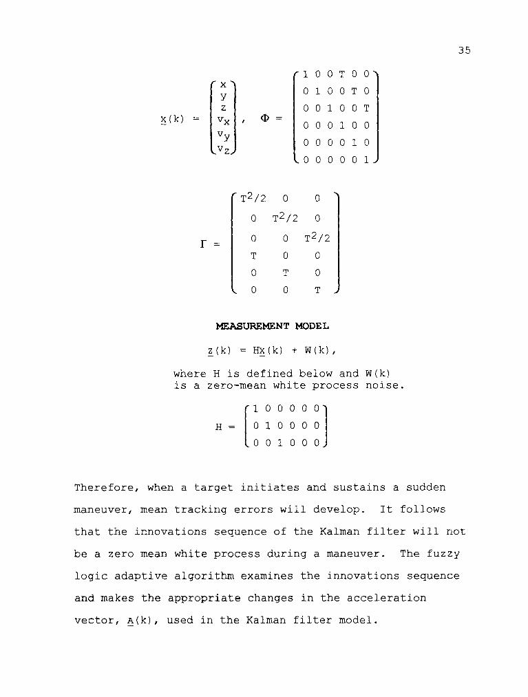
~(k+1) = ~~(k) + r~(k), (5.1 )

where ~(k), ~ and r are defined below.~(k) is an acceleration vector.T is the sampling period.

35

1 0 0 T 0 0xy 0 1 o 0 T 0

z 0 0 1 0 0 T~ (k) = Vx <l> =

0 0 0 1 0 0vy

0 0 0 0 1 0Vz

0 0 0 0 0 1

T2/2 0 0

0 T2/2 0

r 0 0 T2/2=

T 0 0

0 T 0

0 0 T

MEASUREMENT MODEL

~(k) = H~(k) + W(k),

where H is defined below and W(k)is a zero-mean white process noise.

[

100000]H = 0 1 000 0

001 000

Therefore, when a target initiates and sustains a sudden

maneuver, mean tracking errors will develop. It follows

that the innovations sequence of the Kalman filter will not

be a zero mean white process during a maneuver. The fuzzy

logic adaptive algorithm examines the innovations sequence

and makes the appropriate changes in the acceleration

vector, ~(k), used in the Kalman filter model.

36

V.2 Target Simulation

The target's motion is simulated using Equation 5.1 and

a sampling period of 0.1 seconds. The acceleration vector,

~(k), has three components as shown below [15].

The acceleration of the target in the x direction has an

average value of ax and a variance r x ' Similarly, the

acceleration in the y and z directions have an average value

of a y and a z with variances of r y and r z , respectively. A

target maneuver is simulated by changing the average value

of the target's acceleration.

For the purpose of comparison the same maneuver is used

for all four methods listed in Table 5.1. At the beginning

of the track, the target has a zero mean acceleration with a

5 ft/sec 2 variance. Five seconds after track initiation,

the target sustains a maneuver which results in a x=20.0

ft/sec 2 , a y=15.0 ft/sec2 and a z=10.0 ft/sec 2 .

37

LINGUISTIC FUZZY NUMBER OF RESULTSVARIABLES SUBSETS RULES

ERROR LARGE NEGATIVE LARGE

1 MEDIUM NEGATIVE 25 OVERSHOOT.

SMALL

MEDIUM POSITIVE F'AST RISE TIME.

LARGE POSITIVE

LONG SETTLING

CHANGE IN ERROR LARGE NEGATIVE TIME.

MEDIUM NEGATIVE

SHALL LARGE:

MEDIUM NEGATIVE OSCILLATIONS

LARGE POSITIVE:

TIME AVERI\GE LARGE NEGATIVE NO OVERSHOOT.

2 ERROR MEDIUM NEGATIVE 13SMALL LONG RISE TIME.

MEDIUH POSITIVE

LARGE POSITIVE SNALLER

SETTLING TIME.

CHANGE IN TIME NEGATIVE:

AVERAGE ERROR SMALL SMALL

POSITIVE OSCILLIITIONS.

TIME AVERAGE LARGE NEGATIVE NO OVERSHOOT.

3 ERROR MEDIUM NEGATIVE 13SMALL F'AST RISE TIME.

MEDIUM POSITIVE

LARGE NEGATIVE SMALLER

SETTLING TIME.

CHANGE IN TIME NEGATIVE

AVERAGE ERROR SMALL SMALL

POSITIVE OSCILLATIONS.

MAGNITUDE OF' LARGE VERY SMALL4 AVER}\.GE ERROR MEDIUM LARGE 10 OVERSHOOT.

MEDIUM SMALL

SMALL F'AST RI SE TIME.

SMALL SETTLING

TIME.

CHANGE IN POSITIVE

MAGNITUDE OF SMALL NO

AVERAGE ERROR NEGATIVE: OSCILLATIONS.

Table 5.1 Results of fuzzy logic adaptiveKalman filter.

38

V.3 METHOD 1

The first approach examines the error and change in

error between the current and previous iterations to detect

a maneuver. The assumption is that two consecutive errors

that fall outside the confidence intervals determined by Re

indicate a maneuver. The errors in the x, y, and z

directions are considered separately. For example, if the

current error in the x direction is large and the change in

error in the x direction is large then a maneuver has

occurred in the x direction. Therefore, the algorithm is

executed three times on each iteration.

The linguistic variables error and change in error are

divided into five fuzzy subsets, as shown in Table 5.1. The

procedure for developing the membership functions and

control rules for adjusting the filter acceleration is given

below.

Step 1

Step 2

GOAL OF CONTROL RULES.

The goal of the control rules is to ensurethat the innovation sequence remains insidethe confidence interval.

INITIALIZE MEMBERSHIP FUNCTIONS.

As shown in Table 4.2, the confidenceinterval is a function of Re . Therefore,the membership functions are defined usingEquation 2.1, where the distance function,d(x), is defined to be a decreasingexponential function of Re .

Step 3

step 4

INITIALIZE NONFUZZY CHANGES IN FILTERACCELERATION.

These values are obtained by examining themagnitude of the errors that are producedby various maneuvers.

TEST ALGORITHM.

The algorithm is tested and the performanceis evaluated on the following criterion.

A. Maneuver detection time.B. Rise time.C. Overshoot.D. Settling time.E. Maximum error.

39

Step 5

Step 6

The nonfuzzy changes in filter accelerationare adjusted to get the best possibleresults.

CHANGE MEMBERSHIP FUNCTIONS.

The membership functions are altered toimprove the performance of the filterjudged on the criterion listed in Step 4.

Repeat Steps 4 & 5 until no furtherimprovement is possible.

The membership functions which resulted from using this

procedure are shown in Figure 5.2. The control rules are

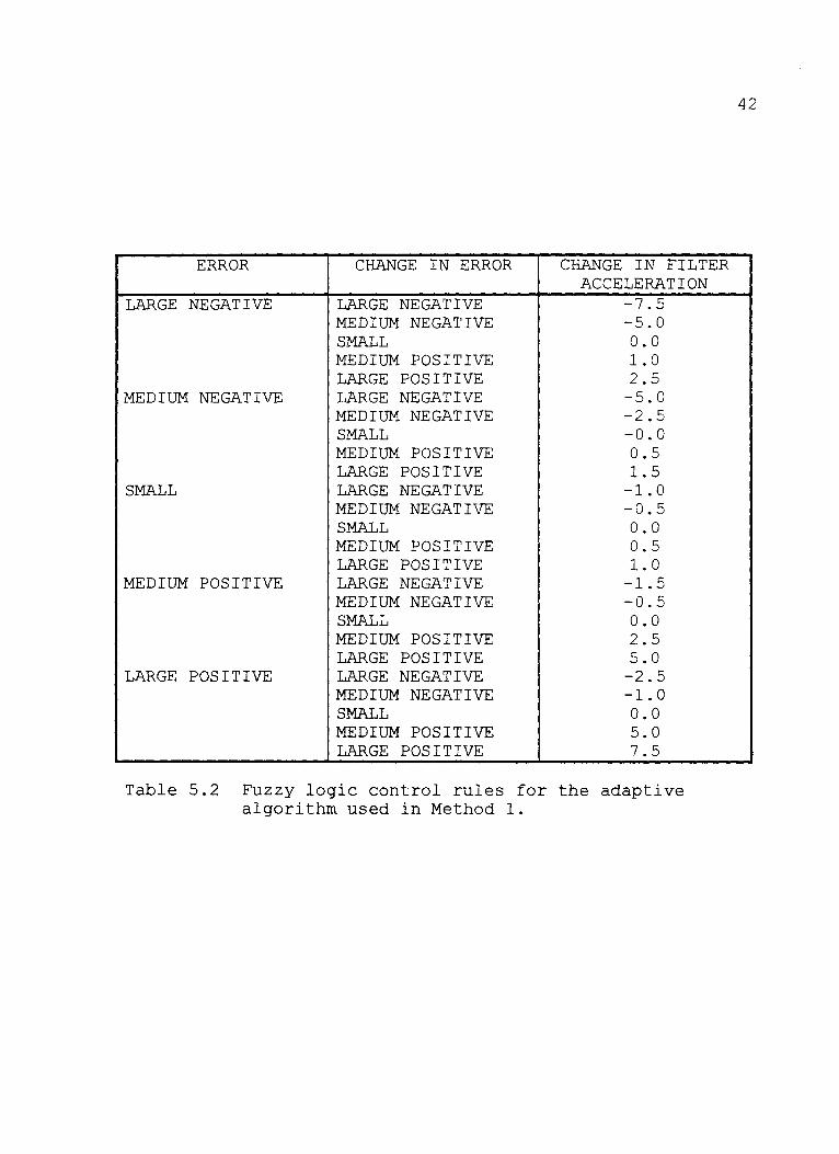
written as standard If-Then statements, an example is:

If the error is LARGE NEGATIVE and thechange in error is LARGE NEGATIVE,

then the change in filter acceleration

is -7.5ft/sec2 .

For convenience, the rule base is written in tabular form in

Table 5.2. The degree of fulfillment for each rule is

40

determined using the center of area method described in

Equation 2.4.

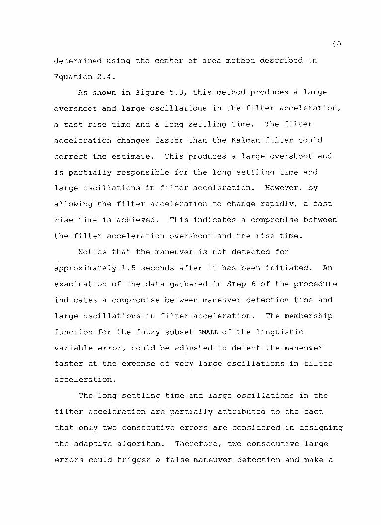
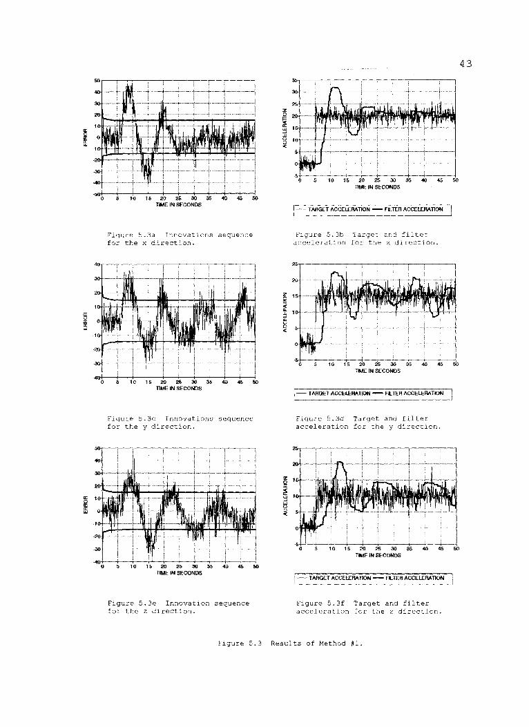
As shown in Figure 5.3, this method produces a large

overshoot and large oscillations in the filter acceleration,

a fast rise time and a long settling time. The filter

acceleration changes faster than the Kalman filter could

correct the estimate. This produces a large overshoot and

is partially responsible for the long settling time and

large oscillations in filter acceleration. However, by

allowing the filter acceleration to change rapidly, a fast

rise time is achieved. This indicates a compromise between

the filter acceleration overshoot and the rise time.

Notice that the maneuver is not detected for

approximately 1.5 seconds after it has been initiated. An

examination of the data gathered in Step 6 of the procedure

indicates a compromise between maneuver detection time and

large oscillations in filter acceleration. The membership

function for the fuzzy subset SMALL of the linguistic

variable error, could be adjusted to detect the maneuver

faster at the expense of very large oscillations in filter

acceleration.

The long settling time and large oscillations in the

filter acceleration are partially attributed to the fact

that only two consecutive errors are considered in designing

the adaptive algorithm. Therefore, two consecutive large

errors could trigger a false maneuver detection and make a

significant change in filter acceleration. These problems

41

are taken into account in the development of the algorithm

used in the second method.

1.6T-----,..------~--.,__----__,

1.4

Figure 5.2a Membership functionsfor the linguisticvariable error.

1.

1.4· ...... . ..

il,:r

•'Jla:'-r-1'.. -w

•

ell:::!w

0.8 ...:::!...0

0.6t··· ... 1. ....;.....w .- ....... ~... .....-.-0

~I

0 o.t ... .. . ..

0.2t··- ........• I··············•

I .I\J .....I ./\.•0.

-l> -4 -2 0. 2 4 6CHANGE IN ERROR (STANDARD DEVATIONSl

Figure 5.2b Membership functionsfor the linguisticvariable change inerror.

Figure 5.2 Membership functions for the linguisticvariables used in Method #1.

42

ERROR CHANGE IN ERROR CHANGE IN FILTERACCELERATION

LARGE NEGATIVE LARGE NEGATIVE -7.5MEDIUM NEGATIVE -5.0SMALL 0.0MEDIUM POSITIVE 1.0LARGE POSITIVE 2.5

MEDIUM NEGATIVE LARGE NEGATIVE -5.0MEDIUM NEGATIVE -2.5SMALL -0.0MEDIUM POSITIVE 0.5LARGE POSITIVE 1.5

SMALL LARGE NEGATIVE -1.0MEDIUM NEGATIVE -0.5SMALL 0.0MEDIUM POSITIVE 0.5LARGE POSITIVE 1.0

MEDIUM POSITIVE LARGE NEGATIVE -1.5MEDIUM NEGATIVE -0.5SMALL 0.0MEDIUM POSITIVE 2.5LARGE POSITIVE 5.0

LARGE POSITIVE LARGE NEGATIVE -2.5MEDIUM NEGATIVE -1.0SMALL 0.0MEDIUM POSITIVE 5.0LARGE POSITIVE 7.5

Table 5.2 Fuzzy logic control rules for the adaptivealgorithm used in Method 1.

1- TARGET ACCElERATION - fLIER ACCElERATION

10 15 20 25 30 35 40 45 50TIME IN SECONDS

5o

4335

30

25Z0

~'"

UJ0 ...

UJcr: U 1'" UUJ <

Figure 5.3a Innovations sequencefor the x direction.

Figure 5.3b Target and filteracceleration for the x direction.

1- TARGET ACCElERATION - fLIER ACCElERATION

zQ:;;ffi 1d8<

10 15 20 25 30 35 40 45 50TIME IN SECONDS

5

-10+-------0-- ---'-1-1\

'"o'"IE

Figure 5.3c Innovations sequencefor the y direction.

Figure 5.3d Target and filteracceleration for the y direction.

40f-----f----ii- ,-----t--------,-----!-----!- ---- +-----,-- I

-1

o 10 15 20 2~ 30 35 4'J 45 50TIME IN SECONDS 1- TARGET ACCElERATION - FLIER ACCElERATION

Figure 5.3e Innovation sequencefor the z direction.

Figure 5.3f Target and filteracceleration for the z direction.

figure 5.3 Results of Method #1.

44

V.4 Method 2

To eliminate false maneuver detections and reduce the

overshoot, settling time, and oscillations in filter

acceleration, the second method examines the time average

error and the change in time average error over the last 10

iterations to determine if a maneuver has occurred. The

average errors in the x, y, and z directions are considered

separately. For example, if the average error over the last

10 iterations in the x direction is large and the change in

average error in the x direction indicates that it is

increasing, then a maneuver has occurred in the x direction.

Therefore, the algorithm is executed three times on each

iteration.

As indicated in Table 5.1, the linguistic variable time

average error is divided into five fuzzy subsets and the

linguistic variable change in time average error is divided

into three fuzzy subsets. A third linguistic variable, no

significant change in filter acceleration, is defined to

ensure that the Kalman filter will have time to correct the

estimate after a large change in filter acceleration. The

change in filter acceleration is defined to be the

difference in filter acceleration at time k and k-10. If

the change in filter acceleration is significant, the Kalman

filter will not be adjusted on the current iteration. The

procedure for developing the membership functions and

45

control rules for adjusting the filter acceleration is given

below.

step 1

Step 2

Step 3

GOAL OF CONTROL RULES.

The goal of the control rules is to ensurethat the mean of the innovation sequence issmall. Ideally, the innovation sequence iszero mean.

INITIALIZE MEMBERSHIP FUNCTIONS.

The membership functions for the fuzzysubsets of the linguistic variables timeaverage error and change in time averageerror are defined using Equation 2.1. Thedistance function, d(x), has the followingform.

d (x) = eA (TAE - B)

The constants A and B are determined byexamining the values of time average errorand change in time average error over thelast 10 iterations that are produced byvarious maneuvers.

The membership function for the linguisticvariable no significant change in filteracceleration is defined using the same typeof distance function. The variable B isset to zero and A is determined by trialand error.


These values are obtained by examining thesize of average errors that are produced byvarious maneuvers.

Step 4

Step 5

Step 6

TEST ALGORITHM.







46

As shown in Figure 5.4, this procedure produces an

S-shaped function that provides a smoother transition from

one fuzzy subset to another. The control rules are written

as a standard If-Then statement. As an example:

If there is no significant change infilter acceleration,then, if the time average error isLARGE NEGATIVE and the change in timeaverage error is NEGATIVE,

then the change in filter accelerationis -4.0 ft/sec2 .

The rule base is given in tabular form in Table 5.3.

Changes in the Kalman filter are only allowed when there has

not been a significant change in filter acceleration.

Therefore, all rules begin as shown in the example above and

47

the linguistic variable no significant change if filter

acceleration is left out of the table. The degree of

fulfillment of each rule is determined and the net change in

filter acceleration is calculated using the center of area

method described in Equation 2.4.

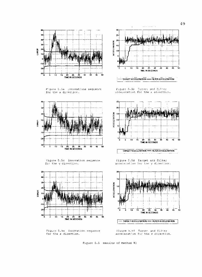
As shown in Figure 5.5, by allowing the Kalman filter

time to correct the estimated position between large changes

in the filter acceleration vector, the overshoot and large

oscillations in filter acceleration are practically

eliminated. However, since the filter acceleration is not

allowed to change rapidly, the rise time has increased.

The maneuver is detected approximately 1.5 seconds

after it has begun, data gathered in Step 6 of the

development procedure indicated a compromise between

maneuver detection time and large oscillations in the filter

acceleration. The membership functions for the linguistic

variable time average error could be adjusted to detect the

error faster at the expense of large oscillations in filter

accelerations. By using the time average error instead of

individual errors to detect maneuvers, the settling time and

oscillations in the filter acceleration are small.

0 .•+············ J0..+ ;. ,

481.

1.4

I

~ 1 "-:E

'" '"a:: a::1

~ ~

; :i0.8 !!! 0.8

15 15

~0.0

~0.0

" 0.4 " 0.4

0,-i---~~-.....-~.....-:-_--.......---1-1 -5 -10 -5 0 5 10 15

THE AVERAGE ERROR /FEEn

0'.....-='-0--_-=-_-=:;__;.--.....-=--1-15 -10 -5 0 5 10 15

CHANOL IN llME AVERAOL ERROR /FEEl)

Figure 5.4a Membership functionsfor the linguistic variabletime average error.

Figure 5.4b Membership functionsfor the linguistic variable

change in time average error.

l-

.

I '\

f :\I \ :

l/ \ :0-10 -8 -6 -4 ~:2 0 2 4 8 10

CHANGE IN FILTER ACCELERATION

Figure 5.4c Membership function for thelinguistic variable no significant change infilter acceleration.

Figure 5.4 Membership functions for the linguistic variables

used in Methods #2 and #3.

TIME AVERAGE CHANGE IN TIME CHANGE IN FILTERERROR AVERAGE ERROR ACCELERATION

LARGE NEGATIVE NEGATIVE -4.0SMALL v.vPOSITIVE 0.0

MEDIUM NEGATIVE NEGATIVE -1.0SMALL 0.0POSITIVE 0.0

SMALL ----- 0.0MEDIUM POSITIVE NEGATIVE 0.0

SMALL 0.0POSITIVE 1.0

LARGE POSITIVE NEGATIVE 0.0SMALL 0.0POSITIVE 4.0

Table 5.3 Fuzzy logic control rules for the adaptivealgorithm used in Method 2.

49

1- TARGET ACCEI£RATION - FLTEFl ACCEI£RAllONI

o 5 10 15 20 25 30 :Is ~o ~ 50TIME IN SECONDS

zo

~wEu«

o 10 15 20 25 30TIME IN SECONDS

40 45 50


-1ot···_······.;.···········;_····_········_+--··...·


o ;; 10 15 20 25 30 35 ~o ~ 50TIME IN SECONDS 1- TARGET ACCEI£RATION FLTER ACCEI£RAllON

Figure 5.5c Innovation sequencefor the y direction.


1- TARGET ACCEI£RATION - fLTEH ACCEI£RAllON

-1

16

zo., 1

~w

~u«

10 20 26 30TIME IN SECONDS

40 ~;; 50

Figure 5.5e Innovation sequencefor the Z direction.

Figure 5.5


Results of Method #2

50

V.5 Method 3

The third method examines the time average error over

the last 10 iterations and the change in time average error

over an adjustable window of L iterations. The error in the

x, y, and z directions are considered separately. If the

average error in the x direction over the last 10 iterations

is not small and the change in average error in the x

direction over the last L iterations indicates that the

average error is increasing, then a maneuver has occurred in

the x direction.

As indicated in Table 5.1, the linguistic variables

time average error and change in time average error are

divided into the same fuzzy subsets and the procedure for

developing the algorithm is the same as that used in Method

2. This procedure produced the same membership functions as

in Method 2, but the nonfuzzy changes in filter acceleration

are different. The control rules are given in tabular form

in Table 5.4. The net change in filter acceleration is

calculated using the center of area method described in

Equation 2.4.

Change in filter acceleration is the difference in

filter acceleration at time k and k-L. After a change in

acceleration of greater then 2.5 ft/sec 2 , the sampling

period is decreased from 0.1 seconds to 0.01 seconds to

allow the filter to correct the estimated position faster.

The results of this method with a window length of 5

51

iterations are shown in Figure 5.6. As indicated, this

method produces a fast rise time, no overshoot, small

oscillations in filter acceleration and a short settling

time. By allowing the sampling period to decrease, the

Kalman filter is able to correct the estimated states faster

after a large change in filter acceleration has occurred.

Notice that the maneuver detection time is still

approximately 1.5 seconds. An attempt to reduce the

maneuver detection time by adjusting the membership

functions results in an increase in filter acceleration

oscillations.

TIME AVERAGE CHANGE IN TIME CHANGE IN FILTERERROR AVERAGE ERROR ACCELERATION

LARGE NEGATIVE NEGATIVE -10.0SMALL 0.0POSITIVE 0.0

MEDIUM NEGATIVE NEGATIVE -2.5SMALL 0.0POSITIVE 0.0

SMALL ----- 0.0MEDIUM POSITIVE NEGATIVE 0.0

SMALL 0.0POSITIVE 2.5

LARGE POSITIVE NEGATIVE 0.0SMALL 0.0POSITIVE 10.0

Table 5.4 Fuzzy logic control rules for the adaptivealgorithm used in Method #3.

52

10 IS 20 25 30 35 40 45 SOTIME IN SECONDS

5o

:10,-----------------,----,

-1

o S 10 IS 20 25 30 3S 40 4S SOTIME IN SECONDS !- TARGET ACCELERATION - fLIER ACCELERATION



-10+----------.-···-----·--;------····..••

o 10 15 20 25 30 35 40 45 50TIME IN SECONDS

o S 10 15 20 2S 30 3S 40 4S SOTIME IN SECONDS !- lAAGEr ACCELERAIION fLIER ACCELERAllON

Figure 5.6c Innovation sequencefor the y direction.


o S 10 15 20 25 30 3!> 40 4S 50lIME IN SECONI)S :1- TARGET ACCELERATION - FLIER ACCELERATION

Figure 5.6e Innovation sequencefor the z direction.


Figure 5.6 Results of Method #3

53

V.6 Method 4

The fourth method examines the magnitude of the time

average error over the last 10 iterations and the change in

magnitude of the average error over an adjustable window of

L iterations. If the magnitude of the time average error

over the last 10 iterations is LARGE and the change in

average error is POSITIVE, then a maneuver has occurred. As

shown in Table 5.1, the linguistic variable magnitude of the

time average error is divided into four fuzzy subsets and

the linguistic variable change in magnitude of the average

error is divided into three fuzzy subsets. A third

linguistic variable, no significant change in filter

acceleration, is defined to ensure that the Kalman filter

has time to correct the estimate after a large change in

filter acceleration.

Change in filter acceleration is the difference in

filter acceleration at time k and k-L. After a change in

filter acceleration greater than 2.5 ft/sec 2 , the sampling

period is decreased from 0.1 seconds to 0.01 seconds to

allow the filter to correct the estimated position faster.

The procedure for developing the algorithm is given below.

Step 1 GOAL OF CONTROL RULES.

The goal of the control rules is to ensurethat the magnitude of the average errorremains small.

Step 2 INITIALIZE MEMBERSHIP FUNCTIONS.54

step 3

Step 4

The membership functions for the fuzzysubsets of the linguistic variablesmagnitude of the time average error and thechange in the magnitude of the averageerror are defined using Equation 2.1. Thedistance function, d(x), has the followingform.

d(x) = eA(ITAEI-B)

The constants A and B are determined byexamining the values of the magnitude oftime average error and change in magnitudeof the average error that are produced byvarious maneuvers.

The membership function for the linguisticvariable no significant change in filteracceleration is the same as that used inMethods 2 and 3.


These values are obtained by examining themagnitudes of the errors that are producedby various maneuvers.

TEST ALGORITHM.




Step 5

Step 6




55

The membership functions which results from using this

procedure are shown in Figure 5.7. The control rules are

written as standard If-Then statements.

If there is no significant change infilter acceleration,then, if the magnitude of the timeaverage error is LARGE and the changein magnitude of the average error isPOSITIVE,then the change in filter acceleration

is 10.0 ft/sec 2 .

The rule base is given in Table 5.5. The degree of

fulfillment of each rule is determined and the magnitude of

the change in filter acceleration is calculated using the

center of area method described in Equation 2.4. The

individual acceleration components are calculated by

multiplying the magnitude of the change in filter

acceleration by the normalized value of the average error.

For example, the change in filter acceleration in the x

direction is calculated as shown below.

I .1FACC I

.1FACC (X) =

nL:DOFi * Wii=l

nL:DOFi

i=l

I.1FAcc l * TAE(x)ITAEI

56

As shown in Figure 5.8, this method produces a fast

rise time, short settling time, very small overshoot and no

oscillations in the filter acceleration. The maneuver

detection time is still approximately 1.5 seconds.

57

o+--~--..;.;;::.._;--~--..,..:::...-I·15 ·10 ·5 0 5 10 15

CHANGE IN MAGNlTIJDE OF AVERAGE ERROR

1.4+ ..- ; , ; .

~ 1.

~ 1 +---.::·1········· ,~;;;.----o;.:+.......... '~;;;.---I::;!!! 0.8...o~ 0.6

g 0'4+·····..···_·..·····,······j,·\·_···,.._······.. ···..···,···········..······,····,,·\·..·..·,·····_..··.. ·....·1

3010 15 20 25MAGNITIJOE OF TIME AVERAGE ERROR

o

.4•

•

.•

'-

lK7 "\ I \ I8·

\/ \L6'

4 .._. ... /'Y"'-'"2) \ Ii\oj \ , ./ \. ..J;\'0.

Figure 5.7a Membership functionfor the linguistic variablemagnitude of time average error.

Figure 5.7b Membership functionfor the linguistic variablechange in magnitude of average error.

1.. ,

•

1.4., ,

, .

if\

I \I \

~. , j \ •

0-10 -8 -6 -4 -2 0 2 4 6 8 10

CHANGE IN FILTER ACCELERATION

Figure 5.7c Membership function forthe linguistic variable no significantchange in filter acceleration.

Figure 5.7 Membership functions for the linguisticvariables used in Method #4.

MAGNITUDE OF CHANGE IN CHANGE IN FILTER_AVERAGE ERROR MAGNITUDE OF ACCELERATION

AVERAGE ERRORLARGE POSITIVE 10.0

SMALL 0.0NEGATIVE 0.0

MEDIUM LARGE POSITIVE 5.0SMALL 0.0NEGATIVE 0.0

MEDIUM SMALL POSITIVE 1.0SMALL 0.0NEGATIVE 0.0

SMALL ----- 0.0

Table 5.5 Fuzzy logic control rules for the adaptivealgorithm used in Method #4.

58

10 15 20 25 30 35 40 45 50TIME IN SECONDS

o S 10 lS 20 2S 30 as 40 'IS 60TIME IN SECONDS 1- TARGET ACCELERATION - fHER ACCELERATION

rigure 5.8a Innovations sequence

for the x direction.

rigure 5.8b Target and filter

acceleration for the x direction.

a: 1

~W

-If}f········+·········i····1

zo~ffi 1...JW(.)(.)

<

o S 10 lS 20 2S 30 as 40 'IS 60TIME IN SECONDS 1- TARGET ACCELERATION - fHER ACCELERATION

Figure 5.8c Innovations sequence

for the y direction.

Figure 5.8d Target and filter

acceleration for the y direction.

!5 1a:a:w

15

10 16 20 25 30lIME IN SECONDS

o 10 lS 20 25 30 as 40 'IS 60TIME IN SECONDS r- TARGET ACCELERATION - fLTER ACCELERATION

I

Figure 5.8e Innovations sequence Figure 5.8f Target and filter

for the z direction. for the z direction.

Figure 5.8 Results of Method #4.

59

V.7 C~UTATIO~ BmIDEN

The methods traditionally used to adapt the Kalman

filter require large amounts of computational time. For

instance, nonlinear filtering, using three unknown

acceleration parameters, would increase the order of the

system from six to nine. It can be shown that the number of

multiplies increases approximately as the cube of the system

order [13J. A sixth order system would have approximately

216 multiplies and a ninth order system would have

approximately 729 multiplies. Therefore, the computational

burden will increase by more than three fold using nonlinear

filtering.

The conditional mean estimate method employs several

parallel filters. Assuming that only two filters are used,

one for no maneuver and one for the largest possible

maneuver, the computational burden would at least double.

For example, for a sixth order system the number of

multiplies is approximately 216. For two parallel filters

the number of multiplies is at least 432. This figure does

not take into account the calculation of the weighting of

each filter.

The number of additional computations required in each

of the four fuzzy logic adaptive algorithms is shown in

Table 5.6. As shown, all four of the methods have a

significantly smaller computational burden than either

nonlinear filtering or conditional mean estimation.

60

METHOD ADDITIONAL COMPUTATIONS REQUIREDNUMBER

1 108 Multiplications and/or Divisions.177 Additions and/or Subtractions.30 Exponential function calculations.




Table 5.6 Computational burden of thefuzzy logic adaptive algorithms.

The fuzzy logic adaptive algorithms provided good

results with Method 4 having the best overall performance

and the least amount of additional computational burden.

61VI. Conclusion

A discussion of fuzzy set theory and fuzzy logic has

been presented. Fuzzy logic has been successfully applied

in a number of different control problems where the system

was either difficult to model or control objectives were

specified qualitatively.

Traditional adaptive Kalman filter techniques were

discussed. These techniques produced good results at the

expense of an increase in computational burden. The

properties of the innovations sequence for a completely

specified Kalman filter were outlined. These properties

were used to develop a fuzzy logic algorithm to adapt the

Kalman filter model.

A procedure for developing a fuzzy logic algorithm was

developed to adapt a Kalman filter model by examining the

innovations sequence. This adaptive approach was applied to

a target tracking system. Four different algorithms were

developed. Method 4 produced the best results. As shown in

Figure 5.8, this method produced a fast rise time, very

small overshoot and no oscillations in filter acceleration

with a very small increase in computational burden.

The major advantages of using fuzzy logic in the

adaptive algorithm is that it does not require a detailed

mathematical model and allows the human judgement of the

engineer to be programmed into the adaptive algorithm. The

62

computational burden was very small as indicated in Table

5.6.

The procedure for developing the membership functions

and control rules was very lengthy. There are very few

guidelines for defining the membership functions and the

tuning process. These were outlined in the algorithm

development procedure for each method, and may need to be

repeated several times before adequate results are achieved.

The fuzzy logic adaptive algorithms that were developed

produced good results for a target tracking system.

However, the maneuver detection time for all of the methods

was approximately 1.5 seconds. Attempts to decrease the

maneuver detection time resulted in larger oscillations in

the filter acceleration. The maneuver detection time could

be reduced by using more fuzzy subsets for each linguistic

variable.

Also the fuzzy logic adaptive algorithm needs to be

tested on a variety of different systems to determine its

overall effectiveness.

REFERENCES

1. Zimmerman, H. J. (1987]. Fuzzy Sets, DecisionMaking, and Expert Systems. Kluwer AcademicPublishers, Boston.

63

2. Zahed, L. A. [1975]. The Concept of aLinguistic Variable and its Application toApproximate Reasoning, Parts 1 & 2. InformationSciences, Vol. 8, pp. 199-249.

3. Zahed, L. A. [1965]. Fuzzy Sets. Informationand Control, Vol. 8, pp. 338-353.

4. Zahed, L. A. [1973]. Outline of a New Approachto the Analysis of Complex Systems and DecisionProcesses. IEEE Transactions on Systems, Man,and Cybernetics, SMC-3, pp. 28-44.

5. Lee, C. C. [1990]. Fuzzy Logic in ControlSystems: Fuzzy Logic Controller. IEEETransactions on Systems, Man, and Cybernetics,SMC-20, pp. 404-435.

6. Kickert, W. J. M. and H. R. van Nauta Lemke(1976]. Application of a Fuzzy Controller in aWarm Water Plant. Automatica, Vol. 12, pp.301-308.

7. Bernard, J. A. (1988]. Use of a Rule-BasedSystem for Process Control. IEEE ControlSystems Magazine, October 1988.

8. Chiu, S., C. Sujeet, D. Moore, and A. Chaudhary[1991]. Fuzzy Logic for Control of Roll andMoment for a Flexible Wing Aircraft. IEEEControl Systems Magazine, June 1991.

9. Li, Y. F. and C. C. Lau [1989]. Development ofFuzzy Algorithms for Servo Systems. IEEEControl Systems Magazine, May 1989.

10. Yoshida, S. and N. Wakabayashi (1992]. A FuzzyLogic Controller for a Rigid Disk Drive. IEEEControl Systems Magazine, June 1992.

6411. Jang, J. and Y. Chen [1990). State Feedback

Effects in Fuzzy Logic Control: A FuzzyModeling Approach. Proceedings of the 1990 IEEEInternational Conference on Systems, Man andCybernetics

12. Candy, J. V. [1986).Model-Based Approach.New York.

Signal Processing: TheMcGraw-Hill Book Company,

13. Brogan, W. L. and J. L. Melsa [No Date). Noteson Theory and Application of AdaptiveEstimation.

14. Blackman, S. S. [1986]. Multiple TargetTracking with Radar Applications. Artech House,Inc., Dedham, MA.

15. Berman, A. and A. Hammer [1991). False AlarmEffects on Estimation in Multitarget Trackers.IEEE Transactions on Aerospace and ElectronicSystems, Vol. 27, pp. 675-681.

fuzzy logic applied to adaptive kalman filtering

Documents