hp loadrunner analysis user guide 3 documentation updates this guide’s title page contains the...
TRANSCRIPT
HP LoadRunner
for the Windows operating systems
Software Version: 9.50
Analysis User Guide
Manufacturing Part Number: T7182-90014
Document Release Date: January 2009
Software Release Date: January 2009
2
Legal Notices
Warranty
The only warranties for HP products and services are set forth in the express warranty statements accompanying such products and services. Nothing herein should be construed as constituting an additional warranty. HP shall not be liable for technical or editorial errors or omissions contained herein.
The information contained herein is subject to change without notice.
Restricted Rights Legend
Confidential computer software. Valid license from HP required for possession, use or copying. Consistent with FAR 12.211 and 12.212, Commercial Computer Software, Computer Software Documentation, and Technical Data for Commercial Items are licensed to the U.S. Government under vendor's standard commercial license.
Third-Party Web Sites
HP provides links to external third-party Web sites to help you find supplemental information. Site content and availability may change without notice. HP makes no representations or warranties whatsoever as to site content or availability.
Copyright Notices
© 1993 - 2009 Mercury Interactive (Israel) Ltd.
Trademark Notices
Java™ is a US trademark of Sun Microsystems, Inc.
Microsoft® and Windows® are U.S. registered trademarks of Microsoft Corporation.
Oracle® is a registered US trademark of Oracle Corporation, Redwood City, California.
UNIX® is a registered trademark of The Open Group.
3
Documentation Updates
This guide’s title page contains the following identifying information:
• Software Version number, which indicates the software version.
• Document Release Date, which changes each time the document is updated.
• Software Release Date, which indicates the release date of this version of the software.
To check for recent updates, or to verify that you are using the most recent edition of a document, go to:
http://h20230.www2.hp.com/selfsolve/manuals
This site requires that you register for an HP Passport and sign-in. To register for an HP Passport ID, go to:
http://h20229.www2.hp.com/passport-registration.html
Or click the New users - please register link on the HP Passport login page.
You will also receive updated or new editions if you subscribe to the appropriate product support service. Contact your HP sales representative for details.
4
Support
You can visit the HP Software Support web site at:
http://www.hp.com/go/hpsoftwaresupport
This web site provides contact information and details about the products, services, and support that HP Software offers.
HP Software Support Online provides customer self-solve capabilities. It provides a fast and efficient way to access interactive technical support tools needed to manage your business. As a valued support customer, you can benefit by using the HP Software Support web site to:
• Search for knowledge documents of interest
• Submit and track support cases and enhancement requests
• Download software patches
• Manage support contracts
• Look up HP support contacts
• Review information about available services
• Enter into discussions with other software customers
• Research and register for software training
Most of the support areas require that you register as an HP Passport user and sign in. Many also require a support contract.
To find more information about access levels, go to:
http://h20230.www2.hp.com/new_access_levels.jsp
To register for an HP Passport ID, go to:
http://h20229.www2.hp.com/passport-registration.html
5
Table of Contents
Welcome to This Guide .......................................................................15How This Guide Is Organized .............................................................15Who Should Read This Guide .............................................................16LoadRunner Documentation ..............................................................16Additional Online Resources...............................................................18
PART I: WORKING WITH ANALYSIS
Chapter 1: Introducing Analysis..........................................................23About Analysis.....................................................................................24Analysis Basics .....................................................................................25Analysis Graphs ...................................................................................27Accessing and Opening Graphs and Reports ......................................30Printing Graphs or Reports..................................................................34Using Analysis Toolbars ......................................................................35Customizing the Layout of Analysis Windows...................................36Analysis API .........................................................................................40WAN Emulation ..................................................................................40
Chapter 2: Configuring Analysis .........................................................41Setting Data Options ...........................................................................41Setting General Options ......................................................................47Setting Database Options ....................................................................50Setting Web Page Breakdown Options................................................57Setting Analyze Transaction Options..................................................58Viewing Session Properties..................................................................59
Table of Contents
6
Chapter 3: Configuring Graph Display ...............................................61Enlarging a Section of a Graph ..........................................................61Configuring Display Options .............................................................62Using the Legend to Configure Display..............................................68Configuring Measurement Options ....................................................71Configuring Columns .........................................................................72Adding Comments, Notes, and Symbols ............................................74Using Templates ..................................................................................76
Chapter 4: Filtering and Sorting Graph Data .....................................79About Filtering Graph Data.................................................................79About Sorting Graph Data...................................................................80Applying Filter and Sort Criteria to Graphs........................................81Filter Conditions .................................................................................83Understanding the Filter Dialog Boxes ...............................................94Additional Filtering Dialog Boxes .......................................................96
Chapter 5: Working with Analysis Graph Data ................................101Determining a Point’s Coordinates...................................................102Drilling Down in a Graph .................................................................102Changing the Granularity of the Data..............................................105Viewing Measurement Trends...........................................................107Auto Correlating Measurements .......................................................108Viewing Graph Data .........................................................................114Viewing and Editing Graph Properties .............................................117
Chapter 6: Viewing Load Test Scenario Information .......................119Viewing the Load Test Scenario Run Time Settings..........................119Viewing Load Test Scenario Output Messages ..................................121
Chapter 7: Cross Result and Merged Graphs ...................................127About Cross Result and Merged Graphs ...........................................127Cross Result Graphs...........................................................................128Generating Cross Result Graphs .......................................................130Merging Graphs ................................................................................131
Chapter 8: Defining Service Level Agreements ................................135About Defining Service Level Agreements ........................................136Defining an SLA Goal Measured Per Time Interval ..........................137Defining an SLA Goal Measured Over the Whole Run.....................145Understanding the Service Level Agreement Dialog Box .................147
Table of Contents
7
Chapter 9: Managing Results Using Quality Center.........................149About Managing Results Using Quality Center ................................149Connecting to and Disconnecting from Quality Center .................150Opening or Creating a Session Using Quality Center .....................154Saving Sessions to a Quality Center Project .....................................156
Chapter 10: Using Analysis with Performance Center .....................157About Using Analysis with Performance Center...............................158Connecting Analysis to Performance Center ...................................159Disconnecting Analysis from Performance Center ..........................161Downloading Result and Session Files ..............................................162Uploading Session Files and Reports.................................................165
Chapter 11: Importing External Data ...............................................173About the Import Data Tool..............................................................173Using the Import Data Tool ..............................................................174Supported File Types .........................................................................178Defining Custom File Formats ..........................................................181Defining Custom Monitor Types for Import ....................................184
PART II: ANALYSIS GRAPHS
Chapter 12: Vuser Graphs ................................................................187About Vuser Graphs ..........................................................................187Running Vusers Graph .....................................................................188Vuser Summary Graph .....................................................................189Rendezvous Graph ............................................................................190
Chapter 13: Error Graphs..................................................................191About Error Graphs ...........................................................................191Error Statistics Graph ........................................................................192Error Statistics (by Description) Graph .............................................193Total Errors per Second Graph .........................................................194Errors per Second Graph ..................................................................195Errors per Second (by Description) Graph ........................................196
Table of Contents
8
Chapter 14: Transaction Graphs .......................................................197About Transaction Graphs ................................................................197Average Transaction Response Time Graph .....................................198Transactions per Second Graph .......................................................201Total Transactions per Second Graph ...............................................202Transaction Summary Graph ...........................................................203Transaction Performance Summary Graph ......................................204Transaction Response Time (Under Load) Graph ............................205Transaction Response Time (Percentile) Graph ...............................206Transaction Response Time (Distribution) Graph ...........................208
Chapter 15: Web Resource Graphs...................................................209About Web Resource Graphs.............................................................210Hits per Second Graph .....................................................................211Throughput Graph ...........................................................................212HTTP Status Code Summary Graph .................................................213HTTP Responses per Second Graph .................................................214Pages Downloaded per Second Graph .............................................217Retries per Second Graph .................................................................219Retries Summary Graph ...................................................................220Connections Graph ..........................................................................221Connections per Second Graph .......................................................222SSLs per Second Graph .....................................................................223
Chapter 16: Web Page Diagnostics Graphs......................................225About Web Page Diagnostics Graphs................................................226Activating the Web Page Diagnostics Graphs ..................................228Page Component Breakdown Graph ...............................................231Page Component Breakdown (Over Time) Graph ...........................233Page Download Time Breakdown Graph .........................................235Page Download Time Breakdown (Over Time) Graph .....................239Time to First Buffer Breakdown Graph ............................................241Time to First Buffer Breakdown (Over Time) Graph ........................243Downloaded Component Size Graph ..............................................245
Chapter 17: User-Defined Data Point Graphs ..................................247About User-Defined Data Point Graphs............................................247Data Points (Sum) Graph .................................................................248Data Points (Average) Graph ............................................................250
Table of Contents
9
Chapter 18: System Resource Graphs...............................................251About System Resource Graphs.........................................................251Windows Resources Graph ...............................................................252UNIX Resources Graph......................................................................256Server Resources Graph .....................................................................258SNMP Resources Graph ....................................................................260Antara FlameThrower Resources Graph ...........................................261SiteScope Graph ................................................................................273
Chapter 19: Network Monitor Graphs..............................................275About Network Monitoring ..............................................................275Understanding Network Monitoring ................................................276Network Delay Time Graph .............................................................277Network Sub-Path Time Graph ........................................................278Network Segment Delay Graph ........................................................279Verifying the Network as a Bottleneck..............................................280
Chapter 20: Firewall Server Monitor Graphs....................................281About Firewall Server Monitor Graphs .............................................281Check Point FireWall-1 Server Graph ..............................................282
Chapter 21: Web Server Resource Graphs........................................285About Web Server Resource Graphs..................................................286Apache Server Graph ........................................................................287Microsoft Information Internet Server (IIS) Graph ..........................289iPlanet/Netscape Server Graph .........................................................291iPlanet (SNMP) Server Graph ............................................................293
Chapter 22: Web Application Server Resource Graphs....................299About Web Application Server Resource Graphs..............................300Ariba Graph ......................................................................................301ATG Dynamo Graph ........................................................................304BroadVision Graph ...........................................................................308ColdFusion Graph ............................................................................316Fujitsu INTERSTAGE Graph .............................................................318iPlanet (NAS) Graph ..........................................................................319Microsoft Active Server Pages (ASP) Graph ......................................328Oracle9iAS HTTP Server Graph ........................................................329SilverStream Graph ...........................................................................334WebLogic (SNMP) Graph .................................................................336WebLogic (JMX) Graph ....................................................................339WebSphere Graph .............................................................................342WebSphere Application Server Graph...............................................349WebSphere (EPM) Graph...................................................................353
Table of Contents
10
Chapter 23: Database Server Resource Graphs................................361About Database Server Resource Graphs...........................................361DB2 Graph ........................................................................................362Oracle Graph ....................................................................................377SQL Server Graph .............................................................................380Sybase Graph ....................................................................................382
Chapter 24: Streaming Media Graphs..............................................389About Streaming Media Graphs........................................................389Real Client Graph .............................................................................391Real Server Graph .............................................................................393Windows Media Server Graph .........................................................394Media Player Client Graph................................................................396
Chapter 25: ERP/CRM Server Resource Graphs................................399About ERP/CRM Server Resource Graphs..........................................400SAP Graph .........................................................................................400SAPGUI Graph...................................................................................403SAP Portal Graph ..............................................................................406SAP CCMS Graph ..............................................................................408Siebel Server Manager Graph ...........................................................409Siebel Web Server Graph ..................................................................412PeopleSoft (Tuxedo) Graph ...............................................................414
Chapter 26: Java Performance Graphs..............................................417About Java Performance Graphs .......................................................417J2EE Graph ........................................................................................418
Table of Contents
11
Chapter 27: Application Component Graphs ...................................421About Microsoft COM+ Performance Graphs...................................422About Microsoft .NET CLR Performance Graphs..............................422Microsoft COM+ Graph ....................................................................423COM+ Breakdown Graph..................................................................427COM+ Average Response Time Graph ..............................................429COM+ Call Count Graph ..................................................................431COM+ Call Count Distribution Graph .............................................433COM+ Call Count Per Second Graph ...............................................435COM+ Total Operation Time Graph.................................................437COM+ Total Operation Time Distribution Graph ............................439.NET Breakdown Graph.....................................................................441.NET Average Response Time Graph.................................................443.NET Call Count Graph .....................................................................444.NET Call Count Distribution Graph ................................................446.NET Call Count per Second Graph ..................................................447.NET Total Operation Time Distribution Graph...............................448.NET Total Operation Time Graph....................................................449.NET Resources Graph .......................................................................450
Chapter 28: Application Deployment Solutions Graphs ..................455About Application Deployment Solutions Graphs ...........................455Citrix MetaFrame XP Graph..............................................................456
Chapter 29: Middleware Performance Graphs.................................465About Middleware Performance Graphs...........................................465Tuxedo Resources Graph ..................................................................466IBM WebSphere MQ Graph .............................................................469
Chapter 30: Infrastructure Resources Graphs...................................473About Infrastructure Resources Graphs.............................................473Network Client Graph.......................................................................474
Table of Contents
12
PART III: ANALYSIS REPORTS
Chapter 31: Understanding Analysis Reports...................................479About Analysis Reports......................................................................480Viewing Summary Reports ...............................................................481SLA Reports........................................................................................489Analyzing Transactions .....................................................................491Creating HTML Reports ....................................................................499Working with Transaction Reports ...................................................500Scenario Execution Report ...............................................................503Failed Transaction Report .................................................................503Failed Vuser Report ...........................................................................504Data Point Report .............................................................................504Detailed Transactions Reports...........................................................506Transaction Performance by Vuser Report .......................................507
Chapter 32: Creating a Microsoft Word Report ...............................509About the Microsoft Word Report ....................................................509Creating Microsoft Word Reports .....................................................510
PART IV: WORKING WITH DIAGNOSTICS
Chapter 33: Siebel Diagnostics Graphs ............................................523About Siebel Diagnostics Graphs ......................................................524Enabling Siebel Diagnostics ..............................................................525Viewing the Siebel Usage Section of the Summary Report...............526Viewing Siebel Diagnostics Data .......................................................528Available Siebel Diagnostics Graphs .................................................540
Chapter 34: Siebel DB Diagnostics Graphs.......................................547About Siebel DB Diagnostics Graphs ................................................548Enabling Siebel DB Diagnostics.........................................................549Synchronizing Siebel Clock Settings .................................................551Viewing Siebel DB Diagnostics Data .................................................553Available Siebel DB Diagnostics Graphs ...........................................558
Chapter 35: Oracle 11i Diagnostics Graphs......................................563About Oracle 11i Diagnostics Graphs ...............................................564Enabling Oracle 11i Diagnostics .......................................................565Viewing Oracle 11i Diagnostics Data................................................567Available Oracle 11i Diagnostics Graphs ..........................................572
Table of Contents
13
Chapter 36: SAP Diagnostics Graphs ................................................577About SAP Diagnostics Graphs..........................................................578Enabling SAP Diagnostics..................................................................578Viewing SAP Diagnostics Data ..........................................................579Viewing the SAP Diagnostics in the Summary Report......................583SAP Alerts...........................................................................................585Using the SAP Breakdown Options ...................................................589Available SAP Diagnostics Graphs.....................................................592SAP Secondary Graphs.......................................................................600
Chapter 37: J2EE & .NET Diagnostics Graphs ...................................605About J2EE & .NET Diagnostics Graphs............................................606Enabling Diagnostics for J2EE & .NET ..............................................606Viewing J2EE & .NET Diagnostics in the Summary Report ..............607Viewing J2EE & .NET Diagnostics Data ............................................609J2EE & .NET Diagnostics Graphs.......................................................626J2EE & .NET Server Diagnostics Graphs............................................636
PART V: APPENDIXES
Appendix A: Interpreting Analysis Graphs .......................................649Analyzing Transaction Performance .................................................650Using the Web Page Diagnostics Graphs ..........................................652Using Auto Correlation .....................................................................654Identifying Server Problems ..............................................................659Identifying Network Problems ..........................................................660Comparing Scenario Results .............................................................661
Index..................................................................................................663

Table of Contents
14
15
Welcome to This Guide
Welcome to the HP LoadRunner Analysis User Guide. This guide describes how to use the LoadRunner Analysis graphs and reports in order to analyze system performance.
You use Analysis after running a load test scenario in the HP LoadRunner Controller or HP Performance Center.
HP LoadRunner, a tool for performance testing, stresses your entire application to isolate and identify potential client, network, and server bottlenecks.
HP Performance Center implements the capabilities of LoadRunner on an enterprise level.
This chapter includes:
➤ How This Guide Is Organized on page 15
➤ Who Should Read This Guide on page 16
➤ LoadRunner Documentation on page 16
➤ Additional Online Resources on page 18
How This Guide Is Organized
This guide contains the following parts:
Part I Working with Analysis
Introduces LoadRunner Analysis, and describes how you work with Analysis graphs.
Welcome to This Guide
16
Part II Analysis Graphs
Lists the different types of Analysis graphs and explains how to interpret them.
Part III Analysis Reports
Explains Analysis reports and describes how create a report in Word.
Part IV Working with Diagnostics
Explains how to use the Analysis graphs to identify and pinpoint performance problems in Siebel, Oracle, SAP, J2EE, and .NET environments.
Part V Appendixes
Contains additional information about using HP LoadRunner Analysis.
Who Should Read This Guide
This guide is for the following users of LoadRunner:
➤ Performance Engineers
➤ Project Manager
Readers of this guide should be moderately knowledgeable about enterprise application development and highly skilled in enterprise system and database administration.
LoadRunner Documentation
LoadRunner includes a complete set of documentation describing how to use the product. The documentation is available from the help menu and in PDF format. PDFs can be read and printed using Adobe Reader, which can be downloaded from the Adobe Web site (http://www.adobe.com). Printed documentation is also available on demand.
Welcome to This Guide
17
Accessing the Documentation
You can access the documentation as follows:
➤ From the Start menu, click Start > LoadRunner > Documentation and select the relevant document.
➤ From the Help menu, click Documentation Library to open the merged help.
Getting Started Documentation
➤ Readme. Provides last-minute news and information about LoadRunner. You access the Readme from the Start menu.
➤ HP LoadRunner Quick Start provides a short, step-by-step overview and introduction to using LoadRunner. To access the Quick Start from the Start menu, click Start > LoadRunner > Quick Start.
➤ HP LoadRunner Tutorial. Self-paced printable guide, designed to lead you through the process of load testing and familiarize you with the LoadRunner testing environment. To access the tutorial from the Start menu, click Start > LoadRunner > Tutorial.
LoadRunner Guides
➤ HP Virtual User Generator User Guide. Describes how to create scripts using VuGen. The printed version consists of two volumes, Volume I - Using VuGen and Volume II - Protocols, while the online version is a single volume. When necessary, supplement this user guide with the online HP LoadRunner Online Function Reference.
➤ HP LoadRunner Controller User Guide. Describes how to create and run LoadRunner scenarios using the LoadRunner Controller in a Windows environment.
➤ HP LoadRunner Monitor Reference. Describes how to set up the server monitor environment and configure LoadRunner monitors for monitoring data generated during a scenario.
➤ HP LoadRunner Analysis User Guide. Describes how to use the LoadRunner Analysis graphs and reports after running a scenario to analyze system performance.
Welcome to This Guide
18
➤ HP LoadRunner Installation Guide. Explains how to install LoadRunner and additional LoadRunner components, including LoadRunner samples.
LoadRunner References
➤ LoadRunner Function Reference. Gives you online access to all of LoadRunner’s functions that you can use when creating Vuser scripts, including examples of how to use the functions.
➤ Analysis API Reference. This Analysis API set can be used for unattended creating of an Analysis session or for custom extraction of data from the results of a test run under the Controller. You can access this reference from the Analysis Help menu.
➤ LoadRunner Controller Automation COM and Monitor Automation Reference. An interface with which you can write programs to run the LoadRunner Controller and perform most of the actions available in the Controller user interface. You access this reference (automation.chm) from the <LoadRunner Installation>/bin directory.
➤ Error Codes and Troubleshooting. Provides clear explanations and troubleshooting tips for Controller connectivity and Web protocol errors. It also provides general troubleshooting tips for Winsock, SAPGUI, and Citrix protocols.
Additional Online Resources
Troubleshooting & Knowledge Base accesses the Troubleshooting page on the HP Software Support Web site where you can search the Self-solve knowledge base. Choose Help > Troubleshooting & Knowledge Base. The URL for this Web site is http://h20230.www2.hp.com/troubleshooting.jsp.
HP Software Support accesses the HP Software Support Web site. This site enables you to browse the Self-solve knowledge base. You can also post to and search user discussion forums, submit support requests, download patches and updated documentation, and more. Choose Help > HP Software Support. The URL for this Web site is www.hp.com/go/hpsoftwaresupport.
Welcome to This Guide
19
Most of the support areas require that you register as an HP Passport user and sign in. Many also require a support contract.
To find more information about access levels, go to: http://h20230.www2.hp.com/new_access_levels.jsp
To register for an HP Passport user ID, go to: http://h20229.www2.hp.com/passport-registration.html
HP Software Web site accesses the HP Software Web site. This site provides you with the most up-to-date information on HP Software products. This includes new software releases, seminars and trade shows, customer support, and more. Choose Help > HP Software Web site. The URL for this Web site is www.hp.com/go/software.

Welcome to This Guide
20
Part I
Working with Analysis

22
23
1Introducing Analysis
HP LoadRunner is HP’s tool for application performance testing. LoadRunner stresses your entire application to isolate and identify potential client, network, and server bottlenecks. LoadRunner enables you to test your system under controlled and peak load conditions.
HP LoadRunner Analysis in–depth reports and graphs provide the information that you need to evaluate the performance of your application.
This chapter includes:
➤ About Analysis on page 24
➤ Analysis Basics on page 25
➤ Analysis Graphs on page 27
➤ Accessing and Opening Graphs and Reports on page 30
➤ Printing Graphs or Reports on page 34
➤ Using Analysis Toolbars on page 35
➤ Customizing the Layout of Analysis Windows on page 36
➤ Analysis API on page 40
➤ WAN Emulation on page 40
Chapter 1 • Introducing Analysis
24
About Analysis
During load test scenario execution, Vusers generate result data as they perform their transactions. To monitor the scenario performance during test execution, use the online monitoring tools described in the HP LoadRunner Controller User Guide. To view a summary of the results after test execution, you can use one or more of the following tools:
➤ The Vuser log files contain a full trace of the load test scenario run for each Vuser. These files are located in the scenario results directory. (When you run a Vuser script in standalone mode, these files are placed in the Vuser script directory.) For more information on Vuser log files, refer to the HP Virtual User Generator User Guide.
➤ The Controller Output window displays information about the load test scenario run. If your scenario run fails, look for debug information in this window. For more information, see “Viewing Load Test Scenario Output Messages” on page 121.
➤ The Analysis graphs help you determine system performance and provide information about transactions and Vusers. You can compare multiple graphs by combining results from several load test scenarios or merging several graphs into one.
➤ The Graph Data and Raw Data views display the actual data used to generate the graph in a spreadsheet format. You can copy this data into external spreadsheet applications for further processing.
➤ The Report utilities enable you to view a Summary HTML report for each graph or a variety of Performance and Activity reports. You can create a report as a Microsoft Word document, which automatically summarizes and displays the test’s significant data in graphical and tabular format.
This chapter provides an overview of the graphs and reports that can be generated through Analysis.
Chapter 1 • Introducing Analysis
25
Analysis Basics
This section describes basic concepts that will enhance your understanding of how to work with Analysis.
Creating Analysis Sessions When you run a load test scenario, data is stored in a result file with an .lrr extension. Analysis is the utility that processes the gathered result information and generates graphs and reports.
When you work with the Analysis utility, you work within a session. An Analysis session contains at least one set of scenario results (.lrr file). Analysis stores the display information and layout settings for the active graphs in a file with an .lra extension.
Starting AnalysisYou can open Analysis as an independent application or directly from the Controller. To open Analysis as an independent application, choose one of the following:
➤ Start > Programs > LoadRunner > Applications > Analysis
➤ Start > Programs > LoadRunner > LoadRunner, select the Load Testing tab, and then click Analyze Load Tests.
To open Analysis directly from the Controller, select Results > Analyze Results. This option is only available after running a load test scenario. Analysis takes the latest result file from the current scenario, and opens a new session using these results. You can also instruct the Controller to automatically open Analysis after it completes scenario execution by selecting Results > Auto Load Analysis.
When creating a new session, Analysis prompts you for the scenario result file (.lrr extension) to include in the session. To open an existing Analysis session, you specify an Analysis Session file (.lra extension).
Chapter 1 • Introducing Analysis
26
Collating Execution Results When you run a load test scenario, by default all Vuser information is stored locally on each Vuser host. After scenario execution, the results are automatically collated or consolidated—results from all of the hosts are transferred to the results directory. You disable automatic collation by choosing Results > Auto Collate Results from the Controller window, and clearing the check mark adjacent to the option. To manually collate results, choose Results > Collate Results. If your results have not been collated, Analysis will automatically collate the results before generating the analysis data. For more information about collating results, refer to the HP LoadRunner Controller User Guide.
Viewing Summary Data In large load test scenarios, with results exceeding 100 MB, it can take a long time for Analysis to process the data. While LoadRunner is processing the complete data, you can view a summary of the data.
To view the summary data, choose Tools > Options, and select the Result Collection tab. To process the complete data graphs while you view the summary data, select Display summary data while generating complete data, or select Generate summary data only if you do not want LoadRunner to process the complete Analysis data.
The following graphs are not available when viewing summary data only:
➤ Data Point (Sum)
➤ Error
➤ Network Monitor
➤ Rendezvous
➤ Siebel DB Side Transactions
➤ Siebel DB Side Transactions by SQL Stage
➤ SQL Average Execution Time
➤ Web Page Diagnostics

Chapter 1 • Introducing Analysis
27
Note: Some fields are not available for filtering when you work with summary graphs.
Analysis Graphs
Analysis graphs are divided into the following categories:
➤ Vuser Graphs. Provide information about Vuser states and other Vuser statistics. For more information, see Chapter 12, “Vuser Graphs.”
➤ Error Graphs. Provide information about the errors that occurred during the load test scenario. For more information, see Chapter 13, “Error Graphs.”
➤ Transaction Graphs. Provide information about transaction performance and response time. For more information, see Chapter 14, “Transaction Graphs.”
➤ Web Resource Graphs. Provide information about the throughput, hits per second, HTTP responses per second, number of retries per second, and downloaded pages per second for Web Vusers. For more information, see Chapter 15, “Web Resource Graphs.”
➤ Web Page Diagnostics Graphs. Provide information about the size and download time of each Web page component. For more information, see Chapter 16, “Web Page Diagnostics Graphs.”
➤ User-Defined Data Point Graphs. Provide information about the custom data points that were gathered by the online monitor. For more information, see Chapter 17, “User-Defined Data Point Graphs.”
➤ System Resource Graphs. Provide statistics relating to the system resources that were monitored during the load test scenario using the online monitor. This category also includes graphs for SNMP monitoring. For more information, see Chapter 18, “System Resource Graphs.”
➤ Network Monitor Graphs. Provide information about the network delays. For more information, see Chapter 19, “Network Monitor Graphs.”
Chapter 1 • Introducing Analysis
28
➤ Firewall Server Monitor Graphs. Provide information about firewall server resource usage. For more information, see Chapter 20, “Firewall Server Monitor Graphs.”
➤ Web Server Resource Graphs. Provide information about the resource usage for the Apache, iPlanet/Netscape, iPlanet(SNMP), and MS IIS Web servers. For more information see Chapter 21, “Web Server Resource Graphs.”
➤ Web Application Server Resource Graphs. Provide information about the resource usage for various Web application servers. For more information see Chapter 22, “Web Application Server Resource Graphs.”
➤ Database Server Resource Graphs. Provide information about database resources. For more information, see Chapter 23, “Database Server Resource Graphs.”
➤ Streaming Media Graphs. Provide information about resource usage of streaming media. For more information, see Chapter 24, “Streaming Media Graphs.”
➤ ERP/CRM Server Resource Graphs. Provide information about ERP/CRM server resource usage. For more information, see Chapter 25, “ERP/CRM Server Resource Graphs.”
➤ Java Performance Graphs. Provide information about resource usage of Java-based applications. For more information, see Chapter 26, “Java Performance Graphs.”
➤ Application Component Graphs. Provide information about resource usage of the Microsoft COM+ server and the Microsoft NET CLR server. For more information, see Chapter 27, “Application Component Graphs.”
➤ Application Deployment Solutions Graphs. Provide information about resource usage of the Citrix MetaFrame server. For more information, see Chapter 28, “Application Deployment Solutions Graphs.”
➤ Middleware Performance Graphs. Provide information about resource usage of the Tuxedo and IBM WebSphere MQ servers. For more information, see Chapter 29, “Middleware Performance Graphs.”
Chapter 1 • Introducing Analysis
29
➤ Infrastructure Resources Graphs. Provide information about resource usage of FTP, POP3, SMTP, IMAP, and DNS Vusers on the network client. For more information, see Chapter 30, “Infrastructure Resources Graphs.”
➤ Siebel Diagnostics Graphs. Provide detailed breakdown diagnostics for transactions generated on Siebel Web, Siebel App, and Siebel Database servers. For more information, see Chapter 33, “Siebel Diagnostics Graphs.”
➤ Siebel DB Diagnostics Graphs. Provide detailed breakdown diagnostics for SQLs generated by transactions on the Siebel system. For more information, see Chapter 34, “Siebel DB Diagnostics Graphs.”
➤ Oracle 11i Diagnostics Graphs. Provide detailed breakdown diagnostics for SQLs generated by transactions on the Oracle NCA system. For more information, see Chapter 35, “Oracle 11i Diagnostics Graphs.”
➤ SAP Diagnostics Graphs. Provide detailed breakdown diagnostics for SAP data generated by transactions on the SAP Server. For more information, see Chapter 36, “SAP Diagnostics Graphs.”
➤ J2EE & .NET Diagnostics Graphs. Provide information to trace, time, and troubleshoot individual transactions through J2EE & .NET Web, application, and database servers. For more information, see Chapter 37, “J2EE & .NET Diagnostics Graphs.”
Chapter 1 • Introducing Analysis
30
Accessing and Opening Graphs and Reports
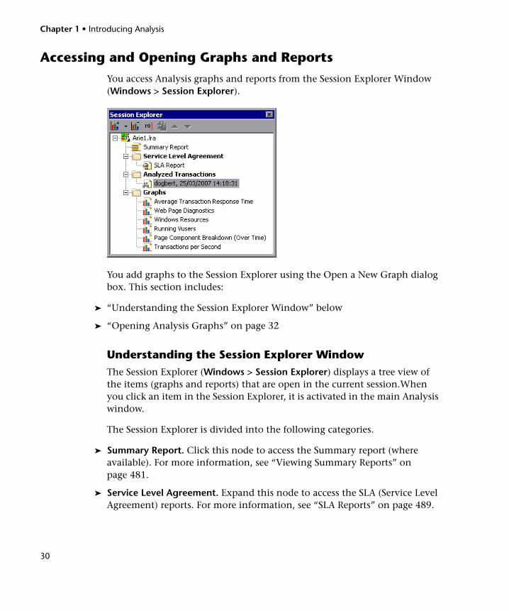
You access Analysis graphs and reports from the Session Explorer Window (Windows > Session Explorer).
You add graphs to the Session Explorer using the Open a New Graph dialog box. This section includes:
➤ “Understanding the Session Explorer Window” below
➤ “Opening Analysis Graphs” on page 32
Understanding the Session Explorer WindowThe Session Explorer (Windows > Session Explorer) displays a tree view of the items (graphs and reports) that are open in the current session.When you click an item in the Session Explorer, it is activated in the main Analysis window.
The Session Explorer is divided into the following categories.
➤ Summary Report. Click this node to access the Summary report (where available). For more information, see “Viewing Summary Reports” on page 481.
➤ Service Level Agreement. Expand this node to access the SLA (Service Level Agreement) reports. For more information, see “SLA Reports” on page 489.
Chapter 1 • Introducing Analysis
31
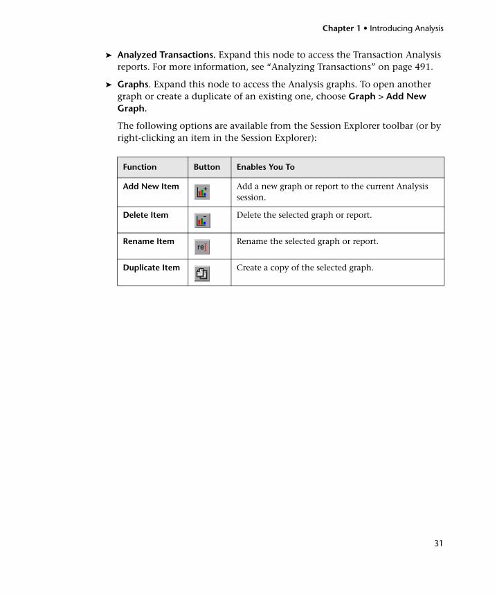
➤ Analyzed Transactions. Expand this node to access the Transaction Analysis reports. For more information, see “Analyzing Transactions” on page 491.
➤ Graphs. Expand this node to access the Analysis graphs. To open another graph or create a duplicate of an existing one, choose Graph > Add New Graph.
The following options are available from the Session Explorer toolbar (or by right-clicking an item in the Session Explorer):
Function Button Enables You To
Add New Item Add a new graph or report to the current Analysis session.
Delete Item Delete the selected graph or report.
Rename Item Rename the selected graph or report.
Duplicate Item Create a copy of the selected graph.
Chapter 1 • Introducing Analysis
32
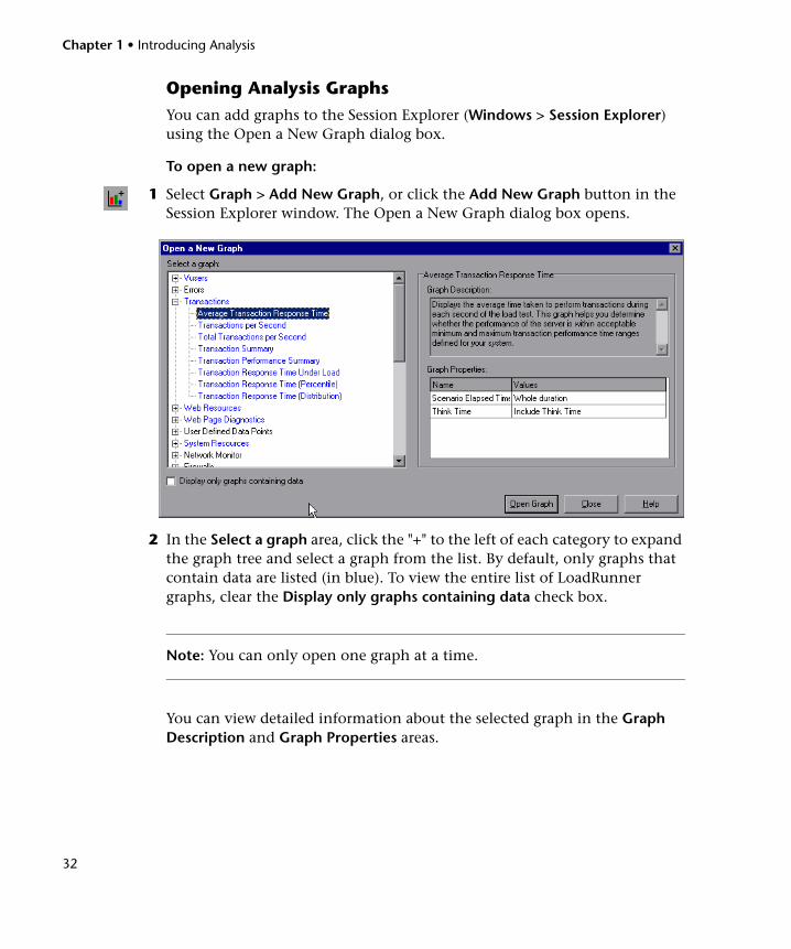
Opening Analysis GraphsYou can add graphs to the Session Explorer (Windows > Session Explorer) using the Open a New Graph dialog box.
To open a new graph:
1 Select Graph > Add New Graph, or click the Add New Graph button in the Session Explorer window. The Open a New Graph dialog box opens.
2 In the Select a graph area, click the "+" to the left of each category to expand the graph tree and select a graph from the list. By default, only graphs that contain data are listed (in blue). To view the entire list of LoadRunner graphs, clear the Display only graphs containing data check box.
Note: You can only open one graph at a time.
You can view detailed information about the selected graph in the Graph Description and Graph Properties areas.
Chapter 1 • Introducing Analysis
33
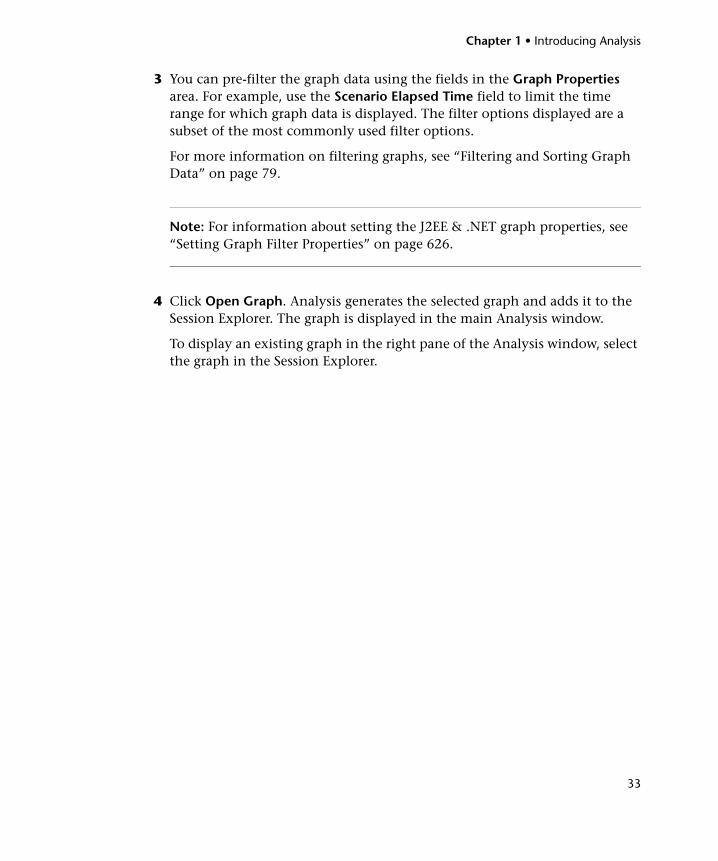
3 You can pre-filter the graph data using the fields in the Graph Properties area. For example, use the Scenario Elapsed Time field to limit the time range for which graph data is displayed. The filter options displayed are a subset of the most commonly used filter options.
For more information on filtering graphs, see “Filtering and Sorting Graph Data” on page 79.
Note: For information about setting the J2EE & .NET graph properties, see “Setting Graph Filter Properties” on page 626.
4 Click Open Graph. Analysis generates the selected graph and adds it to the Session Explorer. The graph is displayed in the main Analysis window.
To display an existing graph in the right pane of the Analysis window, select the graph in the Session Explorer.
Chapter 1 • Introducing Analysis
34
Printing Graphs or Reports
You can print all or selected displayed graphs or reports.
To print graphs or reports:
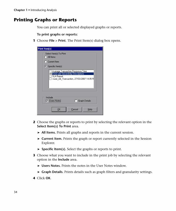
1 Choose File > Print. The Print Item(s) dialog box opens.
2 Choose the graphs or reports to print by selecting the relevant option in the Select Item(s) To Print area.
➤ All Items. Prints all graphs and reports in the current session.
➤ Current Item. Prints the graph or report currently selected in the Session Explorer.
➤ Specific Item(s). Select the graphs or reports to print.
3 Choose what you want to include in the print job by selecting the relevant option in the Include area.
➤ Users Notes. Prints the notes in the User Notes window.
➤ Graph Details. Prints details such as graph filters and granularity settings.
4 Click OK.
Chapter 1 • Introducing Analysis
35
Using Analysis Toolbars
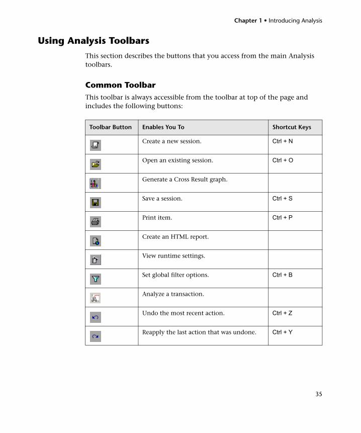
This section describes the buttons that you access from the main Analysis toolbars.
Common Toolbar This toolbar is always accessible from the toolbar at top of the page and includes the following buttons:
Toolbar Button Enables You To Shortcut Keys
Create a new session. Ctrl + N
Open an existing session. Ctrl + O
Generate a Cross Result graph.
Save a session. Ctrl + S
Print item. Ctrl + P
Create an HTML report.
View runtime settings.
Set global filter options. Ctrl + B
Analyze a transaction.
Undo the most recent action. Ctrl + Z
Reapply the last action that was undone. Ctrl + Y
Chapter 1 • Introducing Analysis
36
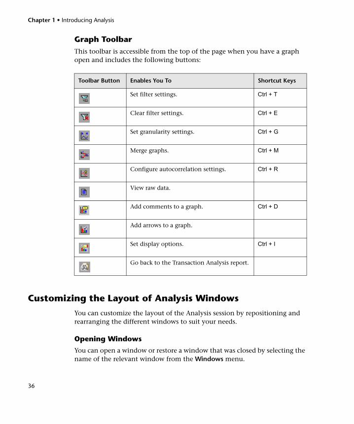
Graph Toolbar This toolbar is accessible from the top of the page when you have a graph open and includes the following buttons:
Customizing the Layout of Analysis Windows
You can customize the layout of the Analysis session by repositioning and rearranging the different windows to suit your needs.
Opening Windows
You can open a window or restore a window that was closed by selecting the name of the relevant window from the Windows menu.
Toolbar Button Enables You To Shortcut Keys
Set filter settings. Ctrl + T
Clear filter settings. Ctrl + E
Set granularity settings. Ctrl + G
Merge graphs. Ctrl + M
Configure autocorrelation settings. Ctrl + R
View raw data.
Add comments to a graph. Ctrl + D
Add arrows to a graph.
Set display options. Ctrl + I
Go back to the Transaction Analysis report.
Chapter 1 • Introducing Analysis
37
Locking/Unlocking the Layout of the Screen
Select Windows > Layout locked to lock or unlock the layout of the screen.
Restoring the Window Placement to the Default Layout
Select Windows > Restore Default Layout to restore the placement of the Analysis windows to their default layout.
Note: This option is available only when no Analysis session is open.
Restoring the Window Placement to the Classic Layout
Select Windows > Restore Classic Layout to restore the placement of the Analysis windows to their classic layout. The classic layout resembles the layout of earlier versions of Analysis.
Note: This option is available only when no Analysis session is open.
Repositioning and Docking Windows
You can reposition any window by dragging it to the desired position on the screen. You can dock a window by dragging the window and using the arrows of the guide diamond to dock the window in the desired position.
Note: Only document windows (graphs or reports) can be docked in the center portion of the screen.
Chapter 1 • Introducing Analysis
38
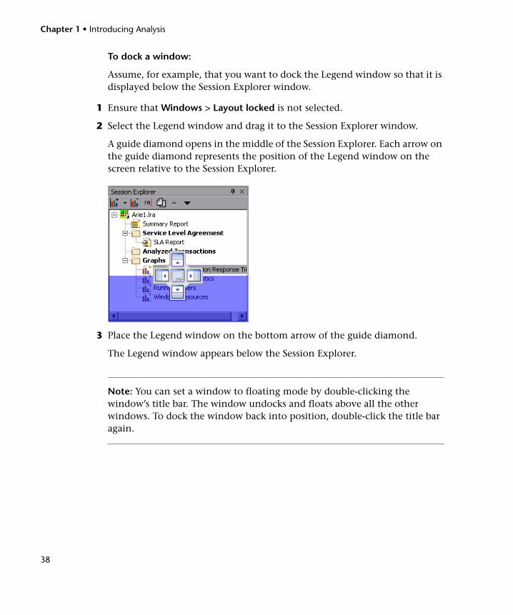
To dock a window:
Assume, for example, that you want to dock the Legend window so that it is displayed below the Session Explorer window.
1 Ensure that Windows > Layout locked is not selected.
2 Select the Legend window and drag it to the Session Explorer window.
A guide diamond opens in the middle of the Session Explorer. Each arrow on the guide diamond represents the position of the Legend window on the screen relative to the Session Explorer.
3 Place the Legend window on the bottom arrow of the guide diamond.
The Legend window appears below the Session Explorer.
Note: You can set a window to floating mode by double-clicking the window’s title bar. The window undocks and floats above all the other windows. To dock the window back into position, double-click the title bar again.
Chapter 1 • Introducing Analysis
39
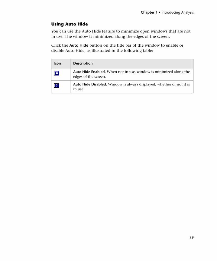
Using Auto Hide
You can use the Auto Hide feature to minimize open windows that are not in use. The window is minimized along the edges of the screen.
Click the Auto Hide button on the title bar of the window to enable or disable Auto Hide, as illustrated in the following table:
Icon Description
Auto Hide Enabled. When not in use, window is minimized along the edges of the screen.
Auto Hide Disabled. Window is always displayed, whether or not it is in use.
Chapter 1 • Introducing Analysis
40
Analysis API
The LoadRunner Analysis API enables you to write programs to perform some of the functions of the Analysis user interface, and to extract data for use in external applications. Among other capabilities, the API allows you to create an analysis session from test results, analyze raw results of an Analysis session, and extract key session measurements for external use. An application can be launched from the LoadRunner Controller at the completion of a test. For more information, see the Analysis API Reference.
WAN Emulation
LoadRunner is integrated with 3rd party software that enables you to accurately test point-to-point performance of WAN-deployed products under real-world network conditions. By installing this 3rd party software on your load generators, you introduce highly probable WAN effects such as latency, packet loss, and link faults over your LAN. As a result of this, your scenario performs the test in an environment that better represents the actual deployment of your application.
You can create more meaningful results by configuring several load generators with the same unique set of WAN effects, and by giving each set a unique location name, for example, London. When viewing scenario results in Analysis, you can group metrics from different load generators according to their location names. For information on grouping metrics according to an emulated location name, see “Applying Filter and Sort Criteria to Graphs” on page 81.
41
2 Configuring Analysis
You configure the main Analysis settings in the Options dialog box (Tools > Options). This chapter describes how to configure Analysis using the tabs in the Options dialog box.
This chapter includes:
➤ Setting Data Options on page 41
➤ Setting General Options on page 47
➤ Setting Database Options on page 50
➤ Setting Web Page Breakdown Options on page 57
➤ Setting Analyze Transaction Options on page 58
➤ Viewing Session Properties on page 59
Setting Data Options
You can configure Analysis to generate and display summary or complete data. When you choose to generate the complete Analysis data, Analysis aggregates the data. Aggregation reduces the size of the database and decreases processing time in large load test scenarios.
You can also configure Analysis to store and display data for the complete duration of the scenario, or for a specified time range only. This decreases the size of the database and thereby decreases processing time.
You use the Result Collection tab of the Options dialog box to configure data options.
Chapter 2 • Configuring Analysis
42
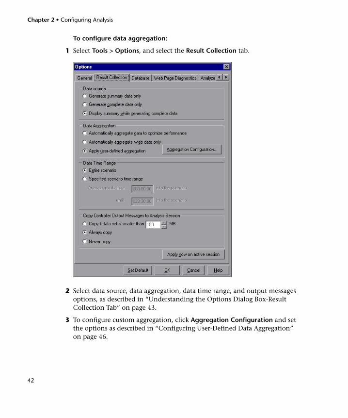
To configure data aggregation:
1 Select Tools > Options, and select the Result Collection tab.
2 Select data source, data aggregation, data time range, and output messages options, as described in “Understanding the Options Dialog Box-Result Collection Tab” on page 43.
3 To configure custom aggregation, click Aggregation Configuration and set the options as described in “Configuring User-Defined Data Aggregation” on page 46.
Chapter 2 • Configuring Analysis
43
Note: All graphs except the Connections and Running Vusers graph will be affected by the time range settings, in both the Summary and Complete Data Analysis modes.
4 Click OK.
To apply the changes to the active session, click Apply now on active session.
Understanding the Options Dialog Box-Result Collection Tab
In large load test scenarios, with results exceeding 100 MB, it will take several minutes for Analysis to process the data. The Result Collection tab of the Options dialog box enables you to indicate to LoadRunner to display a summary of the data, while you wait for the complete data to be processed.
The complete data refers to the result data after it has been processed for use within Analysis. The graphs can be sorted, filtered, and manipulated. The summary data refers to the raw, unprocessed data. The summary graphs contain general information such as transaction names and times, and not all filtering options are available.
If you choose to generate the complete data, Analysis aggregates the data being generated using either built-in data aggregation formulas, or aggregation settings that you define. Data aggregation is necessary in order to reduce the size of the database and decrease processing time in large scenarios.
You can instruct Analysis to display data for the complete duration of the scenario, or for a specified time range only.
You can also choose different options for copying output messages generated by the Controller to the Analysis session.
Chapter 2 • Configuring Analysis
44
You can use this tab to configure the following options:
Data Source
➤ Generate summary data only. View the summary data only. If this option is selected, Analysis will not process the data for advanced use with filtration and grouping.
➤ Generate complete data only. View only the complete data after it has been processed. Do not display the summary data.
➤ Display summary data while generating complete data. View summary data while the complete data is being processed. After the processing, view the complete data. A bar below the graph indicates the complete data generation progress.
For more information about summary data, see “Viewing Summary Data” on page 26
Data Aggregation
➤ Automatically aggregate data to optimize performance. Aggregates data using built-in data aggregation formulas.
➤ Automatically aggregate Web data only. Aggregates Web data only using built-in data aggregation formulas.
➤ Apply user-defined aggregation. Aggregates data using settings you define. Selecting this enables the Aggregation Configuration button. Click this button to define your custom aggregation settings. For more information on user-defined aggregation settings, see “Configuring User-Defined Data Aggregation” on page 46.
Data Time Range
➤ Entire scenario. Displays data for the complete duration of the load test scenario.
➤ Specified scenario time range. Displays data only for the specified time range of the scenario.
➤ Analyze results from X into the scenario. Enter the amount of scenario time you want to elapse (in hh:mm:ss format) before Analysis begins displaying data.
Chapter 2 • Configuring Analysis
45
➤ until X into the scenario. Enter the point in the scenario (in hh:mm:ss format) at which you want Analysis to stop displaying data.
Copy Controller Output Messages to Analysis Session
Choose the relevant option for copying output messages generated by the Controller to the Analysis session. These output messages are displayed in Analysis in the Controller Output Messages window.
➤ Copy if data set is smaller than X MB. Copies the Controller output data to the Analysis session if the data set is smaller than the amount you specify.
➤ Always Copy. Always copies the Controller output data to the Analysis session.
➤ Never Copy. Never copies the Controller output data to the Analysis session.
To apply the settings in the Result Collection tab to the current session, click Apply now to active session. The Controller output data is copied when the Analysis session is saved.
Notes:
➤ It is not recommended to use the Data Time Range feature when analyzing the Oracle 11i and Siebel DB Diagnostics graphs, since the data may be incomplete.
➤ The Data Time Range settings are not applied to the Connections and Running Vusers graphs.
Chapter 2 • Configuring Analysis
46
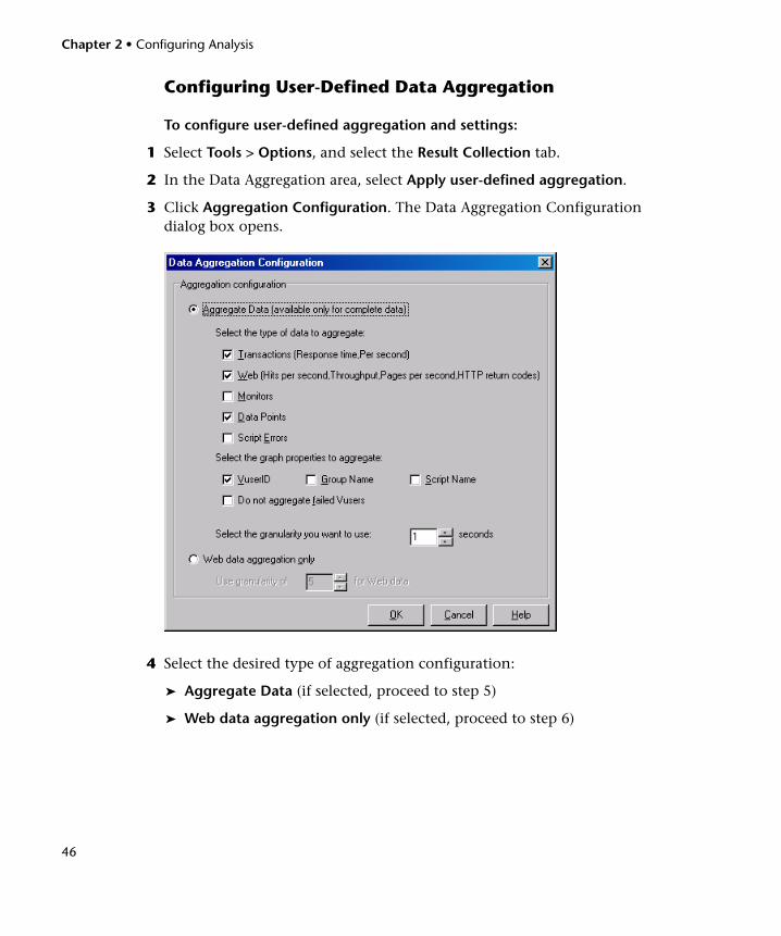
Configuring User-Defined Data Aggregation
To configure user-defined aggregation and settings:
1 Select Tools > Options, and select the Result Collection tab.
2 In the Data Aggregation area, select Apply user-defined aggregation.
3 Click Aggregation Configuration. The Data Aggregation Configuration dialog box opens.
4 Select the desired type of aggregation configuration:
➤ Aggregate Data (if selected, proceed to step 5)
➤ Web data aggregation only (if selected, proceed to step 6)
Chapter 2 • Configuring Analysis
47
5 If you selected Aggregate Data in step 4:
a In the Select the type of data to aggregate list, use the checkboxes to select the types of graphs for which you want to aggregate data. To exclude data from failed Vusers, select Do not aggregate failed Vusers.
b In the Select graph properties to aggregate list, use the checkboxes to select the graph properties you want to aggregate.
Note: You will not be able to drill down on the graph properties you select.
c Specify a custom granularity for the data. To reduce the size of the database, increase the granularity. To focus on more detailed results, decrease the granularity. The minimum granularity is 1 second.
6 If you selected Web aggregation data only in step 4:
➤ In the Use Granularity of X for Web data setting, specify a custom granularity for Web data. By default, Analysis summarizes Web measurements every 5 seconds. To reduce the size of the database, increase the granularity. To focus on more detailed results, decrease the granularity.
7 Click OK.
Setting General Options
You can configure the following general options:
➤ Date storage and display format
➤ File browser directory locations
➤ Temporary file locations
➤ Summary report transaction reporting
You use the General tab of the Options dialog box to set general options.
Chapter 2 • Configuring Analysis
48
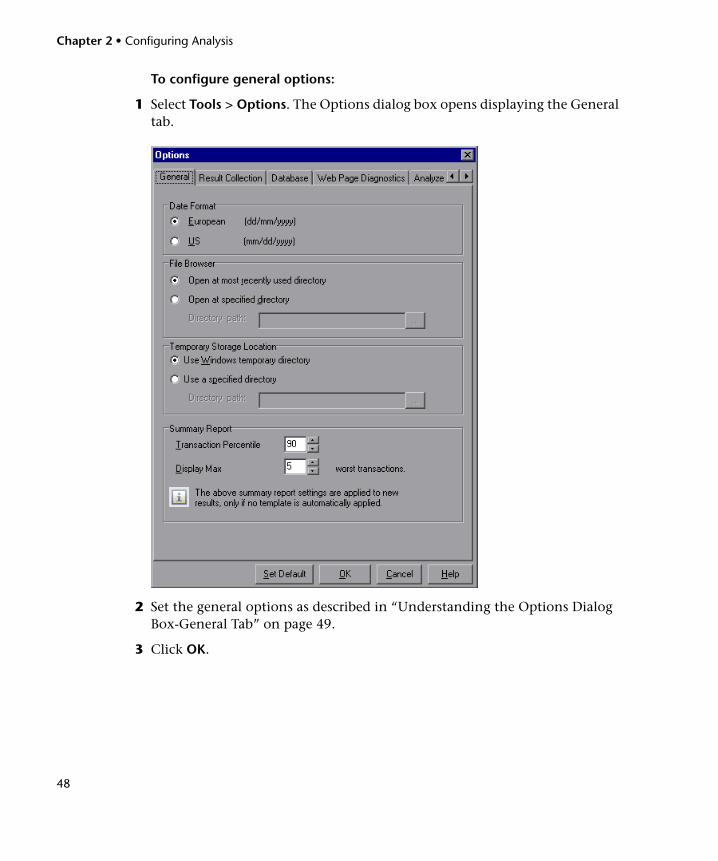
To configure general options:
1 Select Tools > Options. The Options dialog box opens displaying the General tab.
2 Set the general options as described in “Understanding the Options Dialog Box-General Tab” on page 49.
3 Click OK.
Chapter 2 • Configuring Analysis
49
Understanding the Options Dialog Box-General TabYou can use the General tab of the Options dialog box to set the following options:
Date Format
Select a date format for storage and display.
➤ European. Displays the European date format.
➤ US. Displays the U.S. date format.
File Browser
Select the directory location at which you want the file browser to open.
➤ Open at most recently used directory. Opens the file browser at the previously used directory location.
➤ Open at specified directory. Opens the file browser at a specified directory. In the Directory path box, enter the directory location where you want the file browser to open.
Temporary Storage Location
Select the directory location in which you want to save temporary files.
➤ Use Windows temporary directory. Saves temporary files in your Windows temp directory.
➤ Use a specified directory. Saves temporary files in a specified directory. In the Directory path box, enter the directory location in which you want to save temporary files.
Summary Report
Set the following transaction settings in the Summary Report:
➤ Transaction Percentile. The Summary Report contains a percentile column showing the response time of 90% of transactions (90% of transactions that fall within this amount of time). To change the value of the default 90 percentile, enter a new figure in the Transaction Percentile box.
Chapter 2 • Configuring Analysis
50
Since this is an application level setting, the new value is only applied the next time you analyze a result file (File > New).
➤ Display Max. Where a Service Level Agreement (SLA) has been defined, the Summary Report contains the Worst Transactions table that displays the transactions that most exceeded the SLA boundary. The setting here defines how many transactions are displayed in that table. To change this number (for example, to 6), enter a new figure in the Display Max box.
Since this is an application level setting, the new value is only applied the next time you analyze a result file (File > New).
Note: If a template is automatically applied to new sessions, the transaction settings are defined according to the definitions in the template, and not according to those in the Options dialog box. You define template settings in the Template dialog box (Tools > Templates > Apply/Edit Template).
Setting Database Options
You can choose the database in which to store Analysis session result data and you can repair and compress your Analysis results and optimize the database that may have become fragmented.
By default, LoadRunner stores Analysis result data in an Access 2000 database. If your Analysis result data exceeds two gigabytes, it is recommended that you store it on an SQL server or MSDE machine.
This section includes:
➤ “Configuring Database Format Options” below
➤ “Understanding the Options Dialog Box-Database Tab” on page 52
➤ “Advanced Database Options” on page 55
➤ “Importing Data Directly from the Analysis Machine” on page 56
Chapter 2 • Configuring Analysis
51
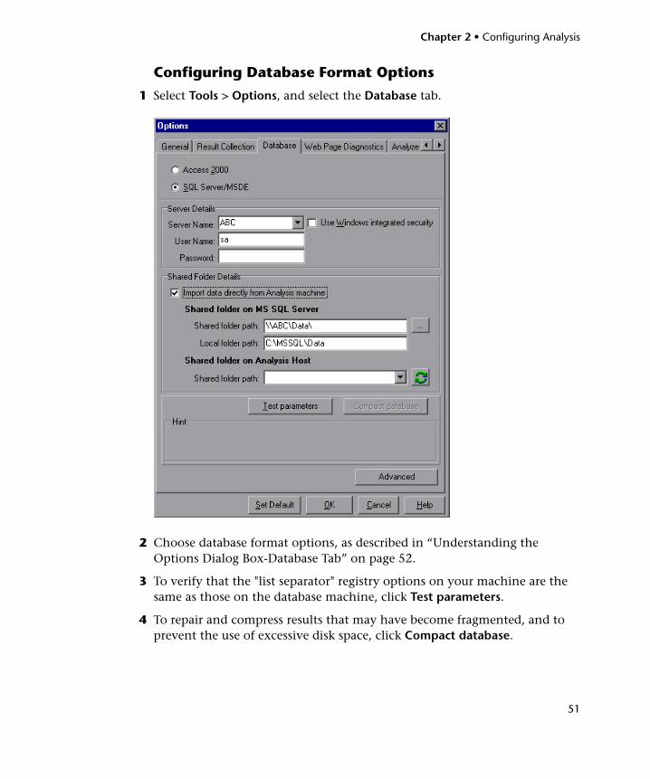
Configuring Database Format Options
1 Select Tools > Options, and select the Database tab.
2 Choose database format options, as described in “Understanding the Options Dialog Box-Database Tab” on page 52.
3 To verify that the "list separator" registry options on your machine are the same as those on the database machine, click Test parameters.
4 To repair and compress results that may have become fragmented, and to prevent the use of excessive disk space, click Compact database.
Chapter 2 • Configuring Analysis
52
Note: Long load test scenarios (duration of two hours or more) will require more time for compacting.
Understanding the Options Dialog Box-Database TabThe Database tab of the Options dialog box enables you to specify the database in which to store Analysis session result data and to configure the way in which CSV files will be imported into the database. If your Analysis result data exceeds two gigabytes, it is recommended that you store it on an SQL server or MSDE machine.
➤ Access 2000. Saves Analysis result data in an Access 2000 database format. This setting is the default.
➤ SQL Server/MSDE. Instructs LoadRunner to save Analysis result data on an SQL server or MSDE machine.
Note: You can install MSDE from the Additional Components link on the product installation disk.
If you choose to store Analysis result data on an SQL server or MSDE machine, you need to complete the following information:
Server Details
➤ Server Name. Select or enter the name of the machine on which the SQL server or MSDE is running.
➤ Use Windows integrated security. Enables you to use your Windows login, instead of specifying a user name and password. By default, the user name "sa"and no password are used for the SQL server.
➤ User Name. Enter the user name for the master database.
➤ Password. Enter the password for the master database.
Chapter 2 • Configuring Analysis
53
Shared Folder Details
➤ Import Data Directly from Analysis machine. Select this option to import data directly from the Analysis machine. For more information about this option, see “Importing Data Directly from the Analysis Machine” on page 56.
➤ Shared Folder on MS SQL Server
➤ Shared folder path. Enter a shared directory on the SQL server/MSDE machine. For example, if your SQL server’s name is fly, enter \\fly\<Analysis database directory>\.
If you did not select the option to import data directly from the Analysis machine, this directory will store permanent and temporary database files. Analysis results stored on an SQL server/MSDE machine can only be viewed on the machine’s local LAN.
If you selected the option to import data directly from the Analysis machine, this directory is used to store an empty database template copied from the Analysis machine.
➤ Local folder path. Enter the real drive and directory path on the SQL server/MSDE machine that correspond to the above shared folder path. For example, if the Analysis database is mapped to an SQL server named fly, and fly is mapped to drive D, enter D:\<Analysis database directory>.
If the SQL server/MSDE and Analysis are on the same machine, the logical storage location and physical storage location are identical.
➤ Shared Folder on Analysis Host
➤ Shared folder path. If you selected the option to import data directly from the Analysis machine, this box is enabled. Enter a shared directory on the Analysis machine. Analysis detects all shared folders on your Analysis machine and displays them in a drop-down list. Select a shared directory from the list. If you can add a new shared directory on your machine, you can click the refresh button to display the updated list of shared folders.
Ensure that the user running the SQL server (by default, SYSTEM) has access rights to this shared folder.
Chapter 2 • Configuring Analysis
54
Analysis creates the CSV files in this directory and the SQL server imports these CSV files from the Analysis machine directly into the database. This directory will store permanent and temporary database files.
➤ Test parameters
➤ For Access. Lets you connect to the Access database and verify that the "list separator" registry options on your machine are the same as those on the database machine.
➤ For SQL server/MSDE. Lets you connect to the SQL server/MSDE machine and see that the shared directory you specified exists on the server, and that you have write permissions on the shared server directory. If so, Analysis synchronizes the shared and physical server directories.
➤ Compact Database. When you configure and set up your Analysis session, the database containing the results may become fragmented. As a result, it will use excessive disk space. The Compact Database button enables you to repair and compress your results and optimize your Access database.
➤ Advanced. Opens the Advanced Options dialog box, allowing you to increase performance when processing LoadRunner results or importing data from other sources. See “Advanced Database Options” below.
Note: If you store Analysis result data on an SQL server/MSDE machine, you must select File > Save As in order to save your Analysis session. To delete your Analysis session, select File > Delete Current Session.
To open a session stored on an SQL server/MSDE machine, the machine must be running and the directory you defined must exist as a shared directory.
Chapter 2 • Configuring Analysis
55
Advanced Database OptionsThe Advanced Options dialog box provides the following options that can increase performance when processing LoadRunner results or importing data from other sources:
➤ Create separate threads for inserting Analysis data into the database. This option may consume a large amount of memory on your database server, and should only be used if you have sufficient memory resources.
➤ Use SQL parameters to utilize the SQL Server memory buffer. This option is only enabled when you store Analysis result data on an SQL server or MSDE machine.
Chapter 2 • Configuring Analysis
56
Importing Data Directly from the Analysis MachineIf you are using an SQL server or MSDE machine to store Analysis result data, you can configure Analysis to import data directly from the Analysis machine.
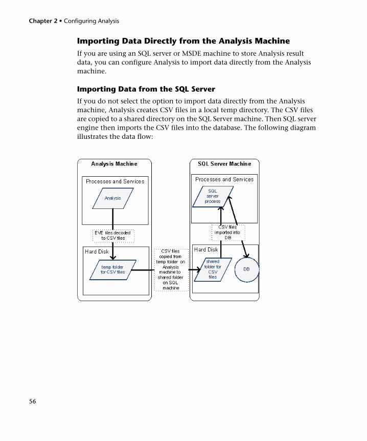
Importing Data from the SQL Server
If you do not select the option to import data directly from the Analysis machine, Analysis creates CSV files in a local temp directory. The CSV files are copied to a shared directory on the SQL Server machine. Then SQL server engine then imports the CSV files into the database. The following diagram illustrates the data flow:
Chapter 2 • Configuring Analysis
57
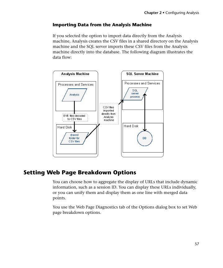
Importing Data from the Analysis Machine
If you selected the option to import data directly from the Analysis machine, Analysis creates the CSV files in a shared directory on the Analysis machine and the SQL server imports these CSV files from the Analysis machine directly into the database. The following diagram illustrates the data flow:
Setting Web Page Breakdown Options
You can choose how to aggregate the display of URLs that include dynamic information, such as a session ID. You can display these URLs individually, or you can unify them and display them as one line with merged data points.
You use the Web Page Diagnostics tab of the Options dialog box to set Web page breakdown options.
Chapter 2 • Configuring Analysis
58
To set the display of URLs with dynamic data:
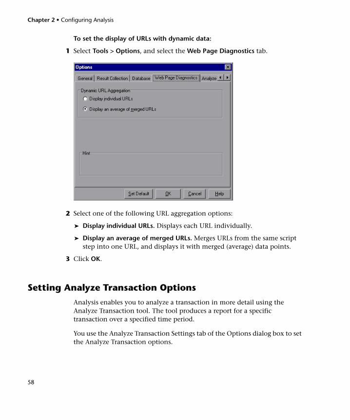
1 Select Tools > Options, and select the Web Page Diagnostics tab.
2 Select one of the following URL aggregation options:
➤ Display individual URLs. Displays each URL individually.
➤ Display an average of merged URLs. Merges URLs from the same script step into one URL, and displays it with merged (average) data points.
3 Click OK.
Setting Analyze Transaction Options
Analysis enables you to analyze a transaction in more detail using the Analyze Transaction tool. The tool produces a report for a specific transaction over a specified time period.
You use the Analyze Transaction Settings tab of the Options dialog box to set the Analyze Transaction options.
Chapter 2 • Configuring Analysis
59
➤ For more information about setting the Analyze Transaction options, see “Understanding the Analyze Transaction Settings” on page 495.
➤ For more information about the Analyze Transaction tool, see “Analyzing Transactions” on page 491.
Viewing Session Properties
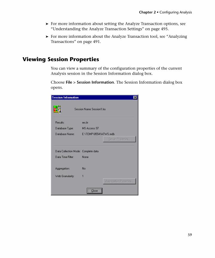
You can view a summary of the configuration properties of the current Analysis session in the Session Information dialog box.
Choose File > Session Information. The Session Information dialog box opens.
Chapter 2 • Configuring Analysis
60
The Session Information dialog box enables you to view the configuration properties of the current Analysis session.
➤ Session Name. Displays the name of the current session.
➤ Results. Displays the name of the LoadRunner result file.
➤ Database Type. Displays the type of database used to store the load test scenario data.
➤ Database Name. Displays the name and directory path of the database.
➤ Server Properties. Displays the properties of the SQL server and MSDE databases.
➤ Data Collection Mode. Indicates whether the session displays complete data or summary data.
➤ Data Time Filter. Indicates whether a time filter has been applied to the session.
➤ Aggregation. Indicates whether the session data has been aggregated.
➤ Web Granularity. Displays the Web granularity used in the session.
➤ Aggregation Properties. Displays the type of data aggregated, the criteria according to which it is aggregated, and the time granularity of the aggregated data.
61
3Configuring Graph Display
Analysis allows you to customize the display of the graphs and measurements in your session so that you can view the data displayed in the most effective way possible.
This chapter includes:
➤ Enlarging a Section of a Graph on page 61
➤ Configuring Display Options on page 62
➤ Using the Legend to Configure Display on page 68
➤ Configuring Measurement Options on page 71
➤ Configuring Columns on page 72
➤ Adding Comments, Notes, and Symbols on page 74
➤ Using Templates on page 76
Enlarging a Section of a Graph
Graphs initially display data representing the entire duration of the load test scenario. You can enlarge any section of a graph to zoom in on a specific period of the scenario run. For example, if a scenario ran for ten minutes, you can enlarge and focus on the scenario events that occurred between the second and fifth minutes.
To zoom in on a section of the graph:
1 Click inside a graph.
2 Move the mouse pointer to the beginning of the section you want to enlarge, but not over a line of the graph.
Chapter 3 • Configuring Graph Display
62
3 Hold down the left mouse button and draw a box around the section you want to enlarge.
4 Release the left mouse button. The section is enlarged.
5 To restore the original view, choose Clear Display Option from the right-click menu.
Configuring Display Options
You can configure graph display options at the following levels:
➤ Basic. Enables you to select the type of graph and the time settings.
➤ Advanced. Enables you to modify the scale and format of each graph.
This section includes:
➤ “Configuring Basic Display Options” on page 63
➤ “Configuring Advanced Graph Display Options” on page 66
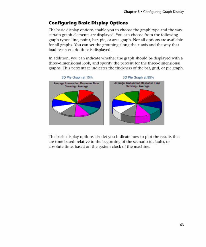
Chapter 3 • Configuring Graph Display
63
Configuring Basic Display OptionsThe basic display options enable you to choose the graph type and the way certain graph elements are displayed. You can choose from the following graph types: line, point, bar, pie, or area graph. Not all options are available for all graphs. You can set the grouping along the x-axis and the way that load test scenario time is displayed.
In addition, you can indicate whether the graph should be displayed with a three-dimensional look, and specify the percent for the three-dimensional graphs. This percentage indicates the thickness of the bar, grid, or pie graph.
The basic display options also let you indicate how to plot the results that are time-based: relative to the beginning of the scenario (default), or absolute time, based on the system clock of the machine.
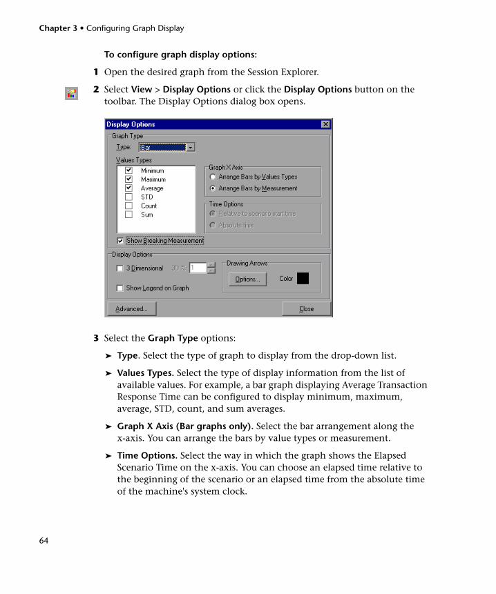
Chapter 3 • Configuring Graph Display
64
To configure graph display options:
1 Open the desired graph from the Session Explorer.
2 Select View > Display Options or click the Display Options button on the toolbar. The Display Options dialog box opens.
3 Select the Graph Type options:
➤ Type. Select the type of graph to display from the drop-down list.
➤ Values Types. Select the type of display information from the list of available values. For example, a bar graph displaying Average Transaction Response Time can be configured to display minimum, maximum, average, STD, count, and sum averages.
➤ Graph X Axis (Bar graphs only). Select the bar arrangement along the x-axis. You can arrange the bars by value types or measurement.
➤ Time Options. Select the way in which the graph shows the Elapsed Scenario Time on the x-axis. You can choose an elapsed time relative to the beginning of the scenario or an elapsed time from the absolute time of the machine's system clock.
Chapter 3 • Configuring Graph Display
65
➤ Show Breaking Measurement. Select this check box to display the name and properties of the breaking measurement at the top of the graph (disabled by default).
4 Select the Display Options:
➤ 3 Dimensional. Select this check box to enable a 3-dimensional display of the graph.
➤ 3D %. Specify a percentage for the 3-dimensional aspect of lines in the graph.
➤ Show Legend on Graph. Select this check box to display a legend at the bottom of the graph.
➤ Drawing Arrows. Allows you to configure the style, color, and width of arrows you draw to highlight graph information.
Click the Draw Arrow button on the toolbar to create display arrows on graphs.
5 (Optional) To set advanced options, click Advanced and set the advanced options as described in “Configuring Advanced Graph Display Options” on page 66.
6 Click Close.
Chapter 3 • Configuring Graph Display
66
Configuring Advanced Graph Display OptionsAdvanced options let you configure the look and feel of your graph as well as its title and the format of the data.
To configure advanced graph display options:
1 Choose View > Display Options or click the Display Options button on the toolbar. The Display Options dialog box opens.
2 Click Advanced. The Editing MainChart dialog box opens.
3 Set the desired advanced display options, as described in the following sections, and click Close.
➤ You can customize the graph layout by setting the Chart and Series preferences. Select the appropriate tab and sub-tab to configure your graph.
For detailed information on setting the Chart and Series preferences, see: “Understanding the Editing MainChart Dialog Box - Chart and Series Tabs” below.
➤ The Export tab enables you to store the current graph to an image file in the format of your choice—BMP, JPG, or EMF. You can also export the graph's data to HTML, Excel, or XML.

Chapter 3 • Configuring Graph Display
67
➤ The Print tab enables you to print only the graph itself without the legend and other data such as the User Notes.
Understanding the Editing MainChart Dialog Box - Chart and Series Tabs
The Chart Tab
The Chart tab of the Editing MainChart dialog box enables you to configure the look and feel of your entire graph. You set Chart preferences using the following tabs:
➤ Series. Select the graph style (bar, line, etc.), the hide/show settings, line and fill color, and the title of the series.
➤ General. Select options for print preview, export, margins, scrolling, and magnification.
➤ Axis. Select which axes to show, as well as their scales, titles, ticks, and position.
➤ Titles. Set the title of the graph, its font, background color, border, and alignment.
➤ Legend. Set all legend related settings, such as position, fonts, and divider lines.
➤ Panel. Show the background panel layout of the graph. You can modify its color, set a gradient option, or specify a background image.
➤ Paging. Set all page related settings, such as amount of data per page, scale, and page numbering. These settings are relevant when the graph data exceeds a single page.
➤ Walls. Set colors for the walls of 3-dimensional graphs.
➤ 3D. Select the 3-dimensional settings, offset, magnification, and rotation angle for the active graph.
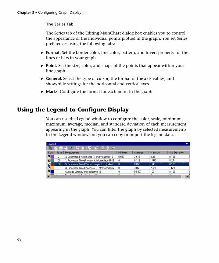
Chapter 3 • Configuring Graph Display
68
The Series Tab
The Series tab of the Editing MainChart dialog box enables you to control the appearance of the individual points plotted in the graph. You set Series preferences using the following tabs:
➤ Format. Set the border color, line color, pattern, and invert property for the lines or bars in your graph.
➤ Point. Set the size, color, and shape of the points that appear within your line graph.
➤ General. Select the type of cursor, the format of the axis values, and show/hide settings for the horizontal and vertical axes.
➤ Marks. Configure the format for each point in the graph.
Using the Legend to Configure Display
You can use the Legend window to configure the color, scale, minimum, maximum, average, median, and standard deviation of each measurement appearing in the graph. You can filter the graph by selected measurements in the Legend window and you can copy or import the legend data.
Chapter 3 • Configuring Graph Display
69
The following options are available from the Legend window toolbar: (Some options are also available by right-clicking a measurement in the Legend window.)
Function Button Enables You To
Show Display a measurement in the graph.
Hide Hide a measurement in the graph.
Show only selected
Display the highlighted measurement only.
Show all Display all the available measurements in the graph.
Filter current graph by selected measurements
Filters the graph by the measurements selected in the Legend window. You can select multiple measurements. To clear the filter, select View > Clear Filter/Group by.
Configure measurements
Opens the Measurement Options dialog box that enables you to configure measurement options (for example, set color and measurement scale). For more information, see “Configuring Measurement Options” on page 71.
Show measurement description
Opens the Measurement Description dialog box that displays the name, monitor type, and description of the selected measurement. For more information, see “Understanding the Measurement Description Dialog Box” on page 70.
Animate selected line
Displays the selected measurement as a flashing line.
Configure columns
Opens the Legend Columns Options dialog box that enables you to configure the columns displayed in the Legend window. For more information, see “Configuring Columns” on page 72.
Copy selected rows to Clipboard
Copies the data that you have selected to the Clipboard. You can paste the data in a text file or a spreadsheet.
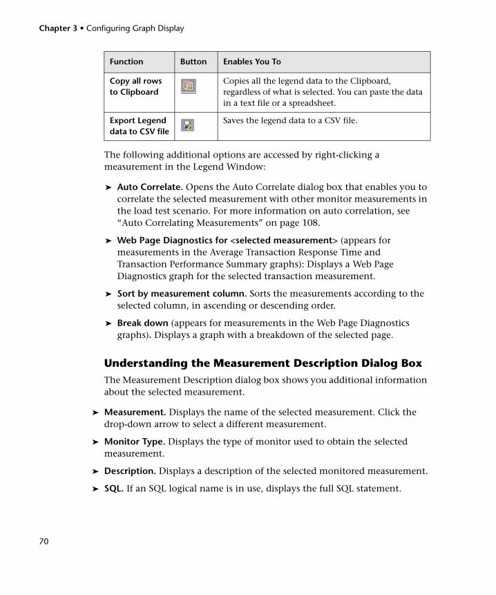
Chapter 3 • Configuring Graph Display
70
The following additional options are accessed by right-clicking a measurement in the Legend Window:
➤ Auto Correlate. Opens the Auto Correlate dialog box that enables you to correlate the selected measurement with other monitor measurements in the load test scenario. For more information on auto correlation, see “Auto Correlating Measurements” on page 108.
➤ Web Page Diagnostics for <selected measurement> (appears for measurements in the Average Transaction Response Time and Transaction Performance Summary graphs): Displays a Web Page Diagnostics graph for the selected transaction measurement.
➤ Sort by measurement column. Sorts the measurements according to the selected column, in ascending or descending order.
➤ Break down (appears for measurements in the Web Page Diagnostics graphs). Displays a graph with a breakdown of the selected page.
Understanding the Measurement Description Dialog BoxThe Measurement Description dialog box shows you additional information about the selected measurement.
➤ Measurement. Displays the name of the selected measurement. Click the drop-down arrow to select a different measurement.
➤ Monitor Type. Displays the type of monitor used to obtain the selected measurement.
➤ Description. Displays a description of the selected monitored measurement.
➤ SQL. If an SQL logical name is in use, displays the full SQL statement.
Copy all rows to Clipboard
Copies all the legend data to the Clipboard, regardless of what is selected. You can paste the data in a text file or a spreadsheet.
Export Legend data to CSV file
Saves the legend data to a CSV file.
Function Button Enables You To
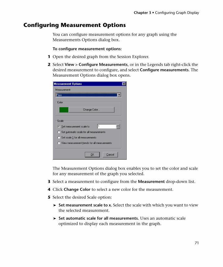
Chapter 3 • Configuring Graph Display
71
Configuring Measurement Options
You can configure measurement options for any graph using the Measurements Options dialog box.
To configure measurement options:
1 Open the desired graph from the Session Explorer.
2 Select View > Configure Measurements, or in the Legends tab right-click the desired measurement to configure, and select Configure measurements. The Measurement Options dialog box opens.
The Measurement Options dialog box enables you to set the color and scale for any measurement of the graph you selected.
3 Select a measurement to configure from the Measurement drop-down list.
4 Click Change Color to select a new color for the measurement.
5 Select the desired Scale option:
➤ Set measurement scale to x. Select the scale with which you want to view the selected measurement.
➤ Set automatic scale for all measurements. Uses an automatic scale optimized to display each measurement in the graph.
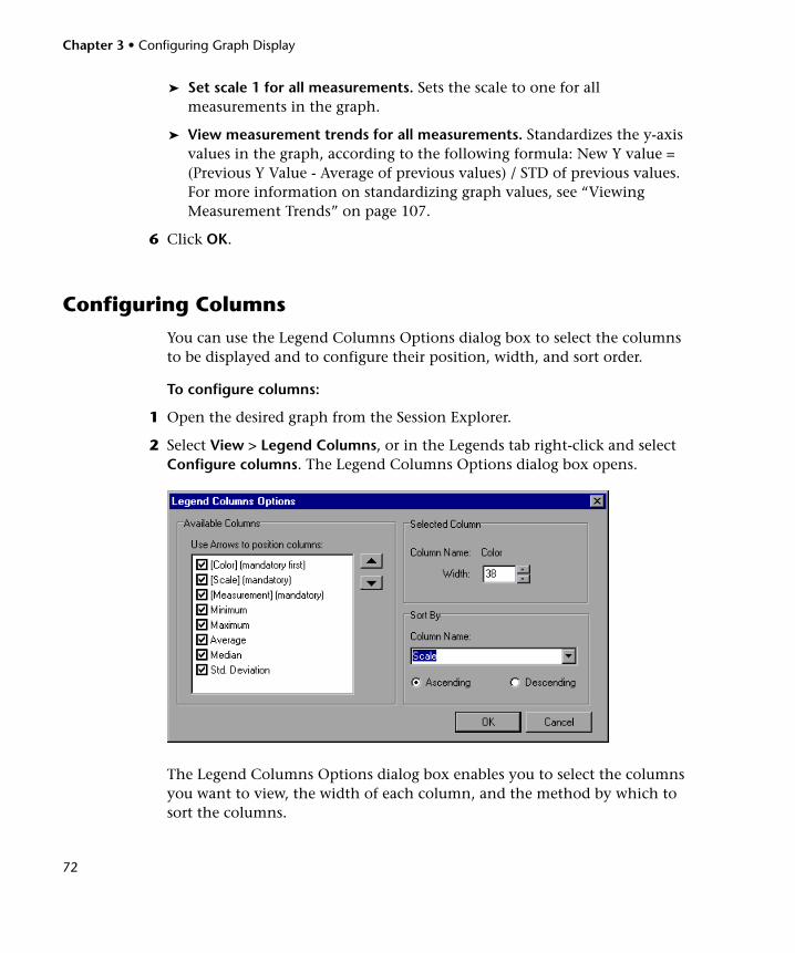
Chapter 3 • Configuring Graph Display
72
➤ Set scale 1 for all measurements. Sets the scale to one for all measurements in the graph.
➤ View measurement trends for all measurements. Standardizes the y-axis values in the graph, according to the following formula: New Y value = (Previous Y Value - Average of previous values) / STD of previous values. For more information on standardizing graph values, see “Viewing Measurement Trends” on page 107.
6 Click OK.
Configuring Columns
You can use the Legend Columns Options dialog box to select the columns to be displayed and to configure their position, width, and sort order.
To configure columns:
1 Open the desired graph from the Session Explorer.
2 Select View > Legend Columns, or in the Legends tab right-click and select Configure columns. The Legend Columns Options dialog box opens.
The Legend Columns Options dialog box enables you to select the columns you want to view, the width of each column, and the method by which to sort the columns.
Chapter 3 • Configuring Graph Display
73
3 In the Available Colums list, select or deselect the check boxes to the left of the column names to show or hide the columns respectively.
Notes:
➤ The Color, Scale, and Measurement columns are mandatory and cannot be deselected.
➤ To rearrange the order in which the columns appear (from left to right), you use the vertical arrows to the right of the Available Columns list to place the columns in the desired order.
4 (Optional) In the Selected Column area, you can modify a selected column’s width by setting the desired pixel value in the Width box.
Note: You can also modify a columns width by dragging its borders in the legend window.
5 In the Sort By area, select the method for sorting measurement data:
➤ From the Column Name drop down list, select the column by which to sort the data.
➤ Select either Ascending or Descending to sort the data in ascending or descending order respectively.
6 Click OK.
Chapter 3 • Configuring Graph Display
74
Adding Comments, Notes, and Symbols
You can tailor your graph by adding comments and arrows to clarify graphical data and specify significant points or areas. You can also enter user notes about specific graphs or reports.
This section includes:
➤ “Using Comments in a Graph” on page 74
➤ “Using Arrows in a Graph” on page 75
➤ “Understanding the User Notes Window” on page 76
Using Comments in a GraphYou can add, edit, format, and delete comments in a graph.
To add a comment:
1 To add a comment, do one of the following:
➤ Right-click in the graph at the location where you want to add the comment, and choose Comments > Add.
➤ Click the Add Comments button on the toolbar. The cursor changes to a drag icon. Click in the graph where you want to position the comment.
The Add Comment dialog box opens.
2 Type a comment in the Text box.
3 Select the desired text alignment and cursor type from the Text alignment and Cursor drop-down lists respectively.
4 Click OK.
To edit, format, or delete a comment:
1 To edit a comment, do one of the following:
➤ Click on the comment.
➤ Right-click in the graph, and choose Comments > Edit.
The Edit Comments dialog box opens
Chapter 3 • Configuring Graph Display
75
2 Perform the desired action as follows:
➤ To edit a comment, select the desired comment in the left pane, and edit the text in the Text box, and change the Text alignment and Cursor settings as desired.
➤ To format a comment, you click the Position, Size, Callout, Format, Text, Gradient, and Shadow tabs.
➤ To delete a comment, select the comment and click Delete, and then Yes.
3 Click Close.
Using Arrows in a GraphYou can add and delete arrows in a graph.
To add an arrow to a graph:
1 Click Draw Arrow button on the toolbar. The cursor changes to a hairline icon.
2 Click the mouse button within the graph to position the base of the arrow.
3 While holding the mouse button down, drag the mouse cursor to position the head of the arrow. Release the mouse button.
4 The arrow’s position can be changed by selecting the arrow itself. Positional boxes appear at the base and head which can be dragged to alternate positions.
To delete an arrow from a graph:
1 Select the arrow by clicking on it. Positional boxes appear at the base and head of the arrow.
2 Press Delete.
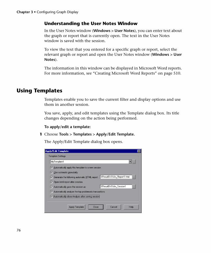
Chapter 3 • Configuring Graph Display
76
Understanding the User Notes WindowIn the User Notes window (Windows > User Notes), you can enter text about the graph or report that is currently open. The text in the User Notes window is saved with the session.
To view the text that you entered for a specific graph or report, select the relevant graph or report and open the User Notes window (Windows > User Notes).
The information in this window can be displayed in Microsoft Word reports. For more information, see “Creating Microsoft Word Reports” on page 510.
Using Templates
Templates enable you to save the current filter and display options and use them in another session.
You save, apply, and edit templates using the Template dialog box. Its title changes depending on the action being performed.
To apply/edit a template:
1 Choose Tools > Templates > Apply/Edit Template.
The Apply/Edit Template dialog box opens.
Chapter 3 • Configuring Graph Display
77
2 Enter template options, as described in “Understanding the Template Dialog Box” on page 78.
3 Click Apply Template to apply the template settings to the current session and close the dialog box, or click Close to save the template settings without applying them to the current session.
To save a template:
1 Choose Tools > Templates > Save as Template.
The Save As Template dialog box opens.
2 Enter template options, as described in “Understanding the Template Dialog Box” on page 78.
3 Click OK.
Chapter 3 • Configuring Graph Display
78
Understanding the Template Dialog BoxThe Template dialog box enables you to set template settings and automatic activity options.
➤ Template Settings. Enter the name of the template you want to create, use, or edit, or click Browse to select a template.
➤ Automatically apply this template to a new session. Applies the template to any new session you create.
➤ Use automatic granularity. Applies the default Analysis granularity (one second) to the template. For information about setting Analysis granularity, see “Changing the Granularity of the Data” on page 105.
➤ Generate the following automatic HTML report. Generates an HTML report using the template. Specify or select a report name. For information about generating HTML reports, see “Creating HTML Reports” on page 499.
➤ Open html report after creation. If you selected the option of generating an automatic HTML report, select this option to automatically open the HTML report after it is created.
➤ Automatically save the session as. Automatically saves the session using the template you specify. Specify or select a file name.
➤ Automatically analyze the top problematic transactions. Automatically generates Transaction Analysis reports for the transactions with the worst SLA violations. Reports are generated for a maximum of five transactions. For more information about Transaction Analysis reports, see “Analyzing Transactions” on page 491.
➤ Automatically close Analysis after saving session. Automatically closes Analysis after a session is automatically saved (using the previous option). This prevents the running of multiple instances of Analysis.
79
4Filtering and Sorting Graph Data
You can filter and sort data that is displayed in a graph. You sort and filter graph data using the same dialog box, as described in this chapter.
This chapter includes:
➤ About Filtering Graph Data on page 79
➤ About Sorting Graph Data on page 80
➤ Applying Filter and Sort Criteria to Graphs on page 81
➤ Filter Conditions on page 83
➤ Understanding the Filter Dialog Boxes on page 94
➤ Additional Filtering Dialog Boxes on page 96
About Filtering Graph Data
You can filter graph data to show fewer transactions for a specific segment of the load test scenario. More specifically, you can display four transactions beginning from five minutes into the scenario and ending three minutes before the end of the scenario.
You can filter for a single graph, in all graphs in a load test scenario, or in the summary graph.
The available filter conditions differ for each type of graph. The filter conditions also depend on your scenario. For example, if you only had one group or one load generator machine in your scenario, the Group Name and Load Generator Name filter conditions do not apply.
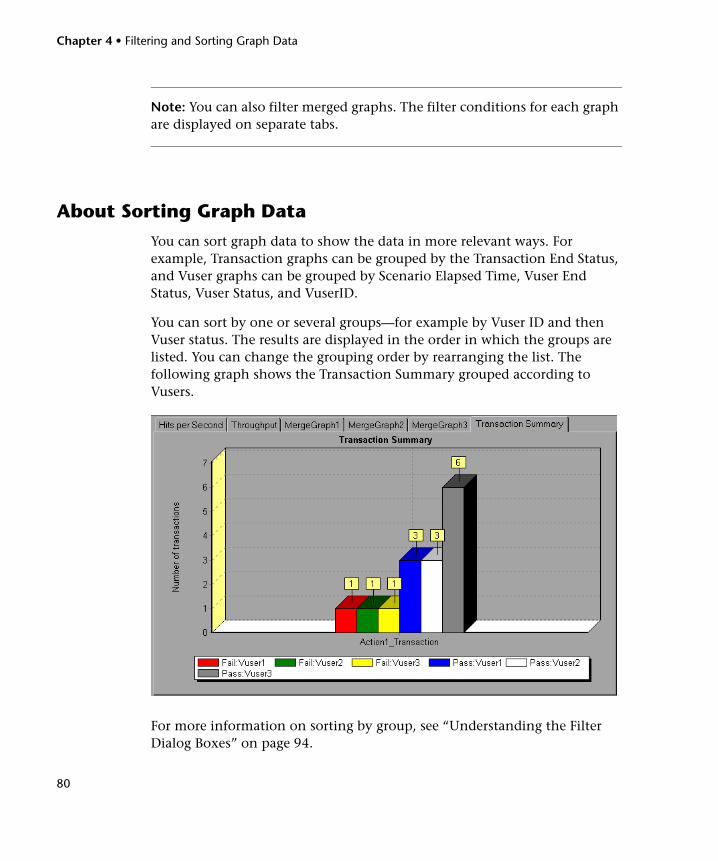
Chapter 4 • Filtering and Sorting Graph Data
80
Note: You can also filter merged graphs. The filter conditions for each graph are displayed on separate tabs.
About Sorting Graph Data
You can sort graph data to show the data in more relevant ways. For example, Transaction graphs can be grouped by the Transaction End Status, and Vuser graphs can be grouped by Scenario Elapsed Time, Vuser End Status, Vuser Status, and VuserID.
You can sort by one or several groups—for example by Vuser ID and then Vuser status. The results are displayed in the order in which the groups are listed. You can change the grouping order by rearranging the list. The following graph shows the Transaction Summary grouped according to Vusers.
For more information on sorting by group, see “Understanding the Filter Dialog Boxes” on page 94.
Chapter 4 • Filtering and Sorting Graph Data
81
Applying Filter and Sort Criteria to Graphs
You apply filter and sort criteria to graphs using the following dialog boxes:
These dialog boxes are all similar, but the name and some of the options differ depending on its use.
In addition to using the above dialog boxes, you can filter the graph by the measurements selected in the Legend window. To do this, select one or more measurement in the Legend window and click the Filter current graph by selected measurements. button in the Legend window toolbar. To clear the filter, select View > Clear Filter/Group by.
Notes:
➤ You can only sort a single graph at a time. Sort settings are only included in the Graph Settings dialog box.
➤ SAP Diagnostics has its own filtering options. For more information, see Chapter 36, “SAP Diagnostics Graphs.”
To set filter conditions:
1 Open the appropriate dialog box by performing one of the following:
➤ To set filter conditions for a single graph, select a graph to filter by clicking the graph tab or clicking the graph name in the Session Explorer, and choose View > Set Filter/Group By or click Set Filter.
To Filter.... Use This Dialog Box
A single graph Graph Settings dialog box (or, for a subset of the filter options, use the Open a New Graph dialog box)
All graphs in a load test scenario
Global Filter dialog box
Summary Report Analysis Summary Filter dialog box
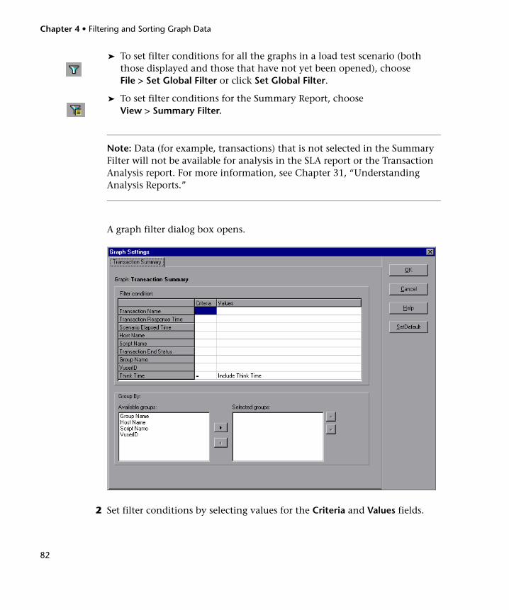
Chapter 4 • Filtering and Sorting Graph Data
82
➤ To set filter conditions for all the graphs in a load test scenario (both those displayed and those that have not yet been opened), choose File > Set Global Filter or click Set Global Filter.
➤ To set filter conditions for the Summary Report, choose View > Summary Filter.
Note: Data (for example, transactions) that is not selected in the Summary Filter will not be available for analysis in the SLA report or the Transaction Analysis report. For more information, see Chapter 31, “Understanding Analysis Reports.”
A graph filter dialog box opens.
2 Set filter conditions by selecting values for the Criteria and Values fields.
Chapter 4 • Filtering and Sorting Graph Data
83
For a description of the filter conditions, see “Filter Conditions” on page 83.
For some filter conditions, one of the following dialog boxes opens, enabling you to specify further filtering details.
➤ Set Dimension Information Dialog Box (described on page 97)
➤ Vuser ID Dialog Box (described on page 98)
➤ Scenario Elapsed Time Dialog Box (described on page 99)
➤ Hierarchical Path Dialog Box (described on page 100)
Set the conditions in the additional dialog box, as described for each dialog box.
3 To sort the graph display by group, select the Group By settings, as described in “Understanding the Filter Dialog Boxes” on page 94.
4 Click OK. The graph dialog box closes and the settings are applied.
Filter Conditions
The available filter conditions differ for each type of graph.
Common Filter Condition Options
The following filter conditions are common to many graphs:
Filter Condition Filters the graph according to...
Host Name The name of the Host machine. Select one or more hosts from the drop down list.
Transaction End Status The end status of a transaction: pass, fail, stop.
Scenario Elapsed Time The time that elapsed from the beginning to the end of the load test scenario. For more information about setting the time range, see “Scenario Elapsed Time Dialog Box” on page 99.
Vuser ID The Vuser ID. For more information, see “Vuser ID Dialog Box” on page 98.
Chapter 4 • Filtering and Sorting Graph Data
84
Vuser Graphs
You can apply the following filter conditions to Vuser graphs:
Error Graphs
You can apply the following filter conditions to Error graphs:
Transaction Graphs
You can apply the following filter conditions to Transaction graphs:
Script Name The name of the script.
Group Name The name of the group to filter by.
Filter Condition Filters the graph according to...
Vuser Status The Vuser status: load, pause, quit, ready, run
Vuser End Status The status of the Vuser at the end of the transaction: error, failed, passed, stopped.
Number of Released Vusers
The number of Vusers that were released.
Rendezvous Name The name of the rendezvous point.
Filter Condition Filters the graph according to...
Error Type The type of error (per error number).
Parent Transaction The parent transaction.
Line Number in Script The line number in the script.
Filter Condition Filters the graph according to...
Transaction Name The name of the transaction.
Filter Condition Filters the graph according to...
Chapter 4 • Filtering and Sorting Graph Data
85
Web Resource Graphs
You can apply the following filter conditions to Web Resources graphs:
Web Page Diagnostics Graphs
You can apply the following filter conditions to Web Page Diagnostics graphs:
Transaction Response Time
The response time of the transaction.
Transaction Hierarchical Path
The hierarchical path of the transaction. For more information on setting this condition, see “Hierarchical Path Dialog Box” on page 100.
Filter Condition Filters the graph according to...
Web Resource Name The name of the Web resource.
Web Resource Value The value of the Web resource.
Web Server Resource Name
The name of the Web Server resource.
Web Server Resource Value
The value of the Web Server resource.
Filter Condition Filters the graph according to...
Component Name The name of the component.
Component Response Time
The response time of the component.
Component DNS Resolution Time
The amount of time the component needs to resolve the DNS name to an IP address, using the closest DNS server.
Component Connection Time
The time taken for the component to establish an initial connection with the Web server hosting the specified URL.
Filter Condition Filters the graph according to...
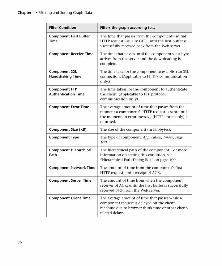
Chapter 4 • Filtering and Sorting Graph Data
86
Component First Buffer Time
The time that passes from the component’s initial HTTP request (usually GET) until the first buffer is successfully received back from the Web server.
Component Receive Time The time that passes until the component’s last byte arrives from the server and the downloading is complete.
Component SSL Handshaking Time
The time take for the component to establish an SSL connection. (Applicable to HTTPS communication only.)
Component FTP Authentication Time
The time taken for the component to authenticate the client. (Applicable to FTP protocol communication only).
Component Error Time The average amount of time that passes from the moment a component’s HTTP request is sent until the moment an error message (HTTP errors only) is returned.
Component Size (KB) The size of the component (in kilobytes).
Component Type The type of component: Application; Image; Page; Text
Component Hierarchical Path
The hierarchical path of the component. For more information on setting this condition, see “Hierarchical Path Dialog Box” on page 100.
Component Network Time The amount of time from the component’s first HTTP request, until receipt of ACK.
Component Server Time The amount of time from when the component receives of ACK, until the first buffer is successfully received back from the Web server.
Component Client Time The average amount of time that passes while a component request is delayed on the client machine due to browser think time or other client-related delays.
Filter Condition Filters the graph according to...
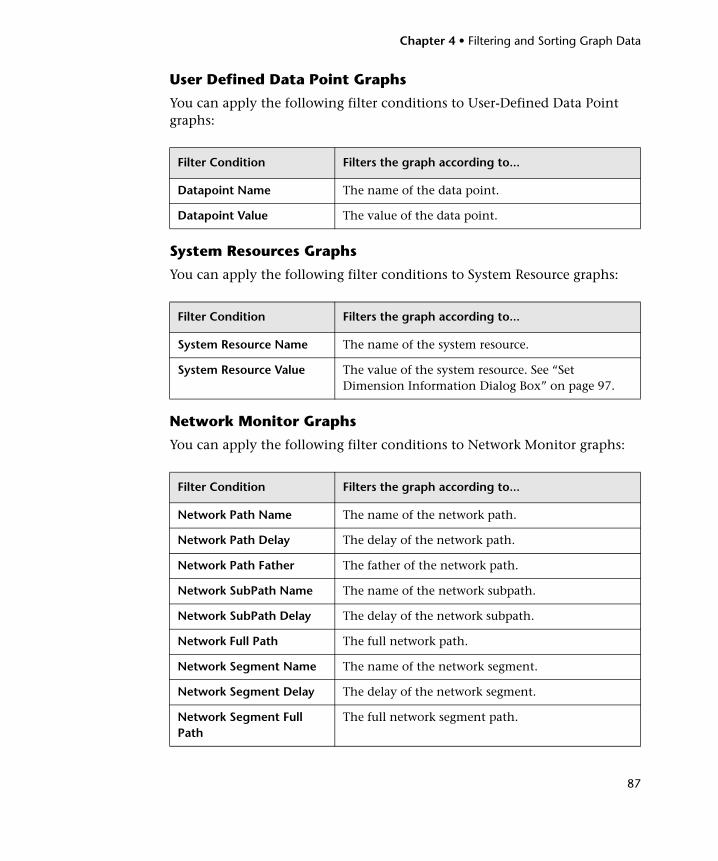
Chapter 4 • Filtering and Sorting Graph Data
87
User Defined Data Point Graphs
You can apply the following filter conditions to User-Defined Data Point graphs:
System Resources Graphs
You can apply the following filter conditions to System Resource graphs:
Network Monitor Graphs
You can apply the following filter conditions to Network Monitor graphs:
Filter Condition Filters the graph according to...
Datapoint Name The name of the data point.
Datapoint Value The value of the data point.
Filter Condition Filters the graph according to...
System Resource Name The name of the system resource.
System Resource Value The value of the system resource. See “Set Dimension Information Dialog Box” on page 97.
Filter Condition Filters the graph according to...
Network Path Name The name of the network path.
Network Path Delay The delay of the network path.
Network Path Father The father of the network path.
Network SubPath Name The name of the network subpath.
Network SubPath Delay The delay of the network subpath.
Network Full Path The full network path.
Network Segment Name The name of the network segment.
Network Segment Delay The delay of the network segment.
Network Segment Full Path
The full network segment path.
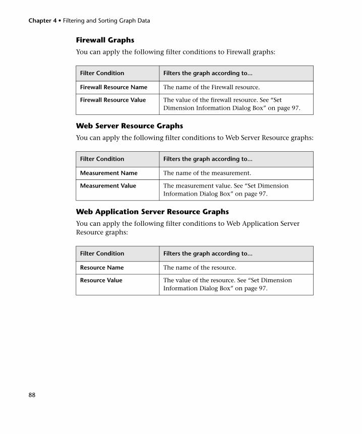
Chapter 4 • Filtering and Sorting Graph Data
88
Firewall Graphs
You can apply the following filter conditions to Firewall graphs:
Web Server Resource Graphs
You can apply the following filter conditions to Web Server Resource graphs:
Web Application Server Resource Graphs
You can apply the following filter conditions to Web Application Server Resource graphs:
Filter Condition Filters the graph according to...
Firewall Resource Name The name of the Firewall resource.
Firewall Resource Value The value of the firewall resource. See “Set Dimension Information Dialog Box” on page 97.
Filter Condition Filters the graph according to...
Measurement Name The name of the measurement.
Measurement Value The measurement value. See “Set Dimension Information Dialog Box” on page 97.
Filter Condition Filters the graph according to...
Resource Name The name of the resource.
Resource Value The value of the resource. See “Set Dimension Information Dialog Box” on page 97.
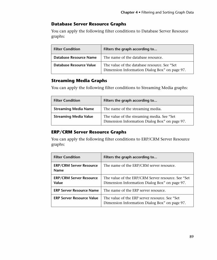
Chapter 4 • Filtering and Sorting Graph Data
89
Database Server Resource Graphs
You can apply the following filter conditions to Database Server Resource graphs:
Streaming Media Graphs
You can apply the following filter conditions to Streaming Media graphs:
ERP/CRM Server Resource Graphs
You can apply the following filter conditions to ERP/CRM Server Resource graphs:
Filter Condition Filters the graph according to...
Database Resource Name The name of the database resource.
Database Resource Value The value of the database resource. See “Set Dimension Information Dialog Box” on page 97.
Filter Condition Filters the graph according to...
Streaming Media Name The name of the streaming media.
Streaming Media Value The value of the streaming media. See “Set Dimension Information Dialog Box” on page 97.
Filter Condition Filters the graph according to...
ERP/CRM Server Resource Name
The name of the ERP/CRM server resource.
ERP/CRM Server Resource Value
The value of the ERP/CRM Server resource. See “Set Dimension Information Dialog Box” on page 97.
ERP Server Resource Name The name of the ERP server resource.
ERP Server Resource Value The value of the ERP server resource. See “Set Dimension Information Dialog Box” on page 97.
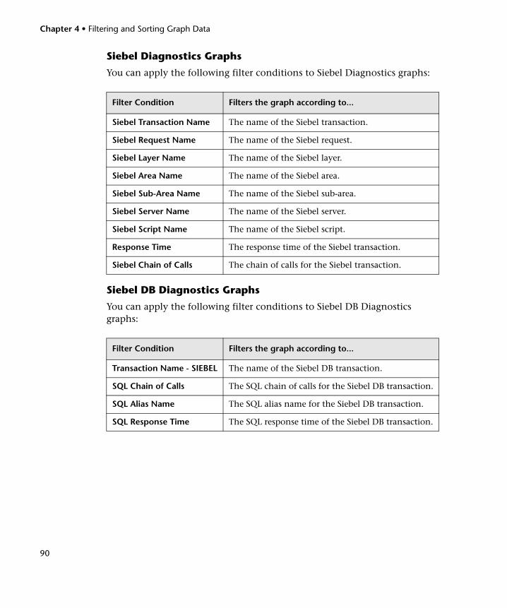
Chapter 4 • Filtering and Sorting Graph Data
90
Siebel Diagnostics Graphs
You can apply the following filter conditions to Siebel Diagnostics graphs:
Siebel DB Diagnostics Graphs
You can apply the following filter conditions to Siebel DB Diagnostics graphs:
Filter Condition Filters the graph according to...
Siebel Transaction Name The name of the Siebel transaction.
Siebel Request Name The name of the Siebel request.
Siebel Layer Name The name of the Siebel layer.
Siebel Area Name The name of the Siebel area.
Siebel Sub-Area Name The name of the Siebel sub-area.
Siebel Server Name The name of the Siebel server.
Siebel Script Name The name of the Siebel script.
Response Time The response time of the Siebel transaction.
Siebel Chain of Calls The chain of calls for the Siebel transaction.
Filter Condition Filters the graph according to...
Transaction Name - SIEBEL The name of the Siebel DB transaction.
SQL Chain of Calls The SQL chain of calls for the Siebel DB transaction.
SQL Alias Name The SQL alias name for the Siebel DB transaction.
SQL Response Time The SQL response time of the Siebel DB transaction.
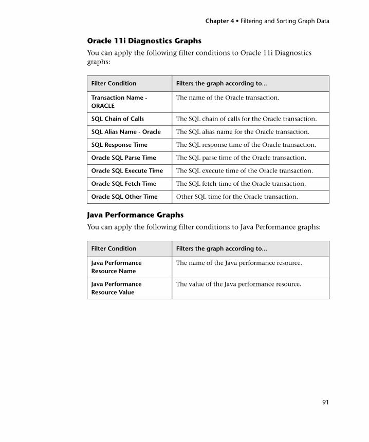
Chapter 4 • Filtering and Sorting Graph Data
91
Oracle 11i Diagnostics Graphs
You can apply the following filter conditions to Oracle 11i Diagnostics graphs:
Java Performance Graphs
You can apply the following filter conditions to Java Performance graphs:
Filter Condition Filters the graph according to...
Transaction Name - ORACLE
The name of the Oracle transaction.
SQL Chain of Calls The SQL chain of calls for the Oracle transaction.
SQL Alias Name - Oracle The SQL alias name for the Oracle transaction.
SQL Response Time The SQL response time of the Oracle transaction.
Oracle SQL Parse Time The SQL parse time of the Oracle transaction.
Oracle SQL Execute Time The SQL execute time of the Oracle transaction.
Oracle SQL Fetch Time The SQL fetch time of the Oracle transaction.
Oracle SQL Other Time Other SQL time for the Oracle transaction.
Filter Condition Filters the graph according to...
Java Performance Resource Name
The name of the Java performance resource.
Java Performance Resource Value
The value of the Java performance resource.
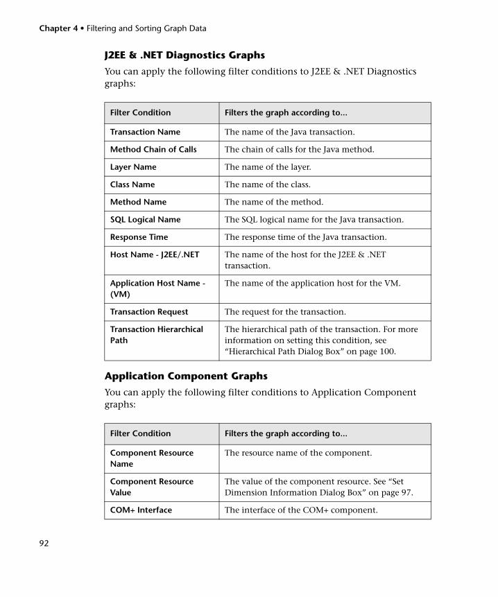
Chapter 4 • Filtering and Sorting Graph Data
92
J2EE & .NET Diagnostics Graphs
You can apply the following filter conditions to J2EE & .NET Diagnostics graphs:
Application Component Graphs
You can apply the following filter conditions to Application Component graphs:
Filter Condition Filters the graph according to...
Transaction Name The name of the Java transaction.
Method Chain of Calls The chain of calls for the Java method.
Layer Name The name of the layer.
Class Name The name of the class.
Method Name The name of the method.
SQL Logical Name The SQL logical name for the Java transaction.
Response Time The response time of the Java transaction.
Host Name - J2EE/.NET The name of the host for the J2EE & .NET transaction.
Application Host Name - (VM)
The name of the application host for the VM.
Transaction Request The request for the transaction.
Transaction Hierarchical Path
The hierarchical path of the transaction. For more information on setting this condition, see “Hierarchical Path Dialog Box” on page 100.
Filter Condition Filters the graph according to...
Component Resource Name
The resource name of the component.
Component Resource Value
The value of the component resource. See “Set Dimension Information Dialog Box” on page 97.
COM+ Interface The interface of the COM+ component.
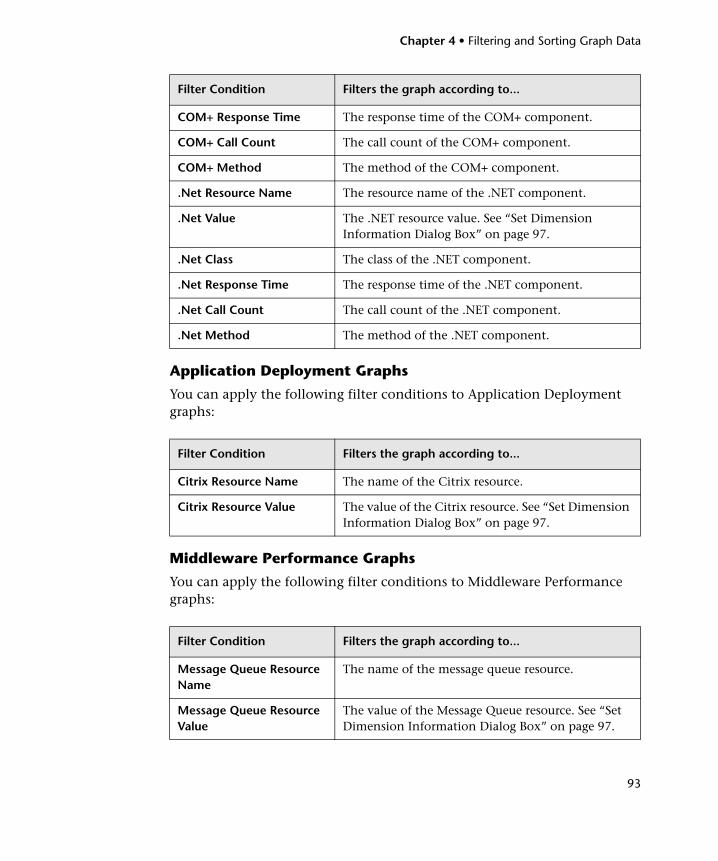
Chapter 4 • Filtering and Sorting Graph Data
93
Application Deployment Graphs
You can apply the following filter conditions to Application Deployment graphs:
Middleware Performance Graphs
You can apply the following filter conditions to Middleware Performance graphs:
COM+ Response Time The response time of the COM+ component.
COM+ Call Count The call count of the COM+ component.
COM+ Method The method of the COM+ component.
.Net Resource Name The resource name of the .NET component.
.Net Value The .NET resource value. See “Set Dimension Information Dialog Box” on page 97.
.Net Class The class of the .NET component.
.Net Response Time The response time of the .NET component.
.Net Call Count The call count of the .NET component.
.Net Method The method of the .NET component.
Filter Condition Filters the graph according to...
Citrix Resource Name The name of the Citrix resource.
Citrix Resource Value The value of the Citrix resource. See “Set Dimension Information Dialog Box” on page 97.
Filter Condition Filters the graph according to...
Message Queue Resource Name
The name of the message queue resource.
Message Queue Resource Value
The value of the Message Queue resource. See “Set Dimension Information Dialog Box” on page 97.
Filter Condition Filters the graph according to...
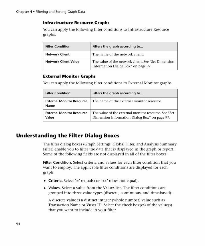
Chapter 4 • Filtering and Sorting Graph Data
94
Infrastructure Resource Graphs
You can apply the following filter conditions to Infrastructure Resource graphs:
External Monitor Graphs
You can apply the following filter conditions to External Monitor graphs
Understanding the Filter Dialog Boxes
The filter dialog boxes (Graph Settings, Global Filter, and Analysis Summary Filter) enable you to filter the data that is displayed in the graph or report. Some of the following fields are not displayed in all of the filter boxes:
Filter Condition. Select criteria and values for each filter condition that you want to employ. The applicable filter conditions are displayed for each graph.
➤ Criteria. Select "=" (equals) or "<>" (does not equal).
➤ Values. Select a value from the Values list. The filter conditions are grouped into three value types (discrete, continuous, and time-based).
A discrete value is a distinct integer (whole number) value such as Transaction Name or Vuser ID. Select the check box(es) of the value(s) that you want to include in your filter.
Filter Condition Filters the graph according to...
Network Client The name of the network client.
Network Client Value The value of the network client. See “Set Dimension Information Dialog Box” on page 97.
Filter Condition Filters the graph according to...
External Monitor Resource Name
The name of the external monitor resource.
External Monitor Resource Value
The value of the external monitor resource. See “Set Dimension Information Dialog Box” on page 97.
Chapter 4 • Filtering and Sorting Graph Data
95
Note: You can filter sub-transactions using the Transaction Hierarchical Path condition. Select "<Transaction_name>" to filter the parent’s sub-transactions; "NONE" to filter for parent transactions; or "Unknown" to filter for sub-transactions whose parents are unknown (usually caused by nesting errors during the session).
Note: Analysis does not support a transaction with character "." as a valid transaction name for J2EE & .NET Diagnostics graphs. (This character is sometimes used as a delimiter in the transaction hierarchy for sub-transactions.) In such cases, Analysis displays the transaction as two separate transactions in the J2EE & .NET Diagnostics graph filter.
A continuous value is a variable dimension that can take any value within the minimum and maximum range limits, such as Transaction Response Time. You set the dimension information for each measurement in the Set Dimension Information Dialog Box.
A time-based value is a value that is based on time relative to the start of the load test scenario. Scenario Elapsed Time is the only condition that uses time-based values. You specify time-based values in the Scenario Elapsed Time Dialog Box.
Group By. Use these settings to sort the graph display by grouping the data. You can group the data by:
➤ Available groups. Select the group by which you want to sort the results, and click the right arrow.
➤ Selected groups. Displays a list of all the selected groups by which the results will be sorted. To remove a value, select it and click the left arrow.
To change the order in which the results are grouped, select the group and click the up or down arrow until the groups are in the desired order.
Chapter 4 • Filtering and Sorting Graph Data
96
Transaction Percentile. The Summary Report contains a percentile column showing the response time of 90% of transactions (90% of transactions that fall within this amount of time). To change the value of the default 90 percentile, enter a new figure in the Transaction Percentile box.
Set Default. Displays the default criteria and values for each filter condition.
Clear All. Deletes all of the information you entered in the dialog box.
Additional Filtering Dialog Boxes
For some filter conditions, one of the following dialog boxes opens to enable you to specify additional filtering details.
➤ Set Dimension Information Dialog Box (described on page 97)
➤ Vuser ID Dialog Box (described on page 98)
➤ Scenario Elapsed Time Dialog Box (described on page 99)
➤ Hierarchical Path Dialog Box (described on page 100)
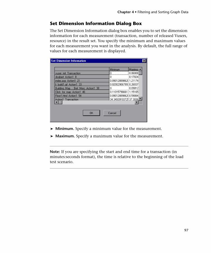
Chapter 4 • Filtering and Sorting Graph Data
97
Set Dimension Information Dialog BoxThe Set Dimension Information dialog box enables you to set the dimension information for each measurement (transaction, number of released Vusers, resource) in the result set. You specify the minimum and maximum values for each measurement you want in the analysis. By default, the full range of values for each measurement is displayed.
➤ Minimum. Specify a minimum value for the measurement.
➤ Maximum. Specify a maximum value for the measurement.
Note: If you are specifying the start and end time for a transaction (in minutes:seconds format), the time is relative to the beginning of the load test scenario.
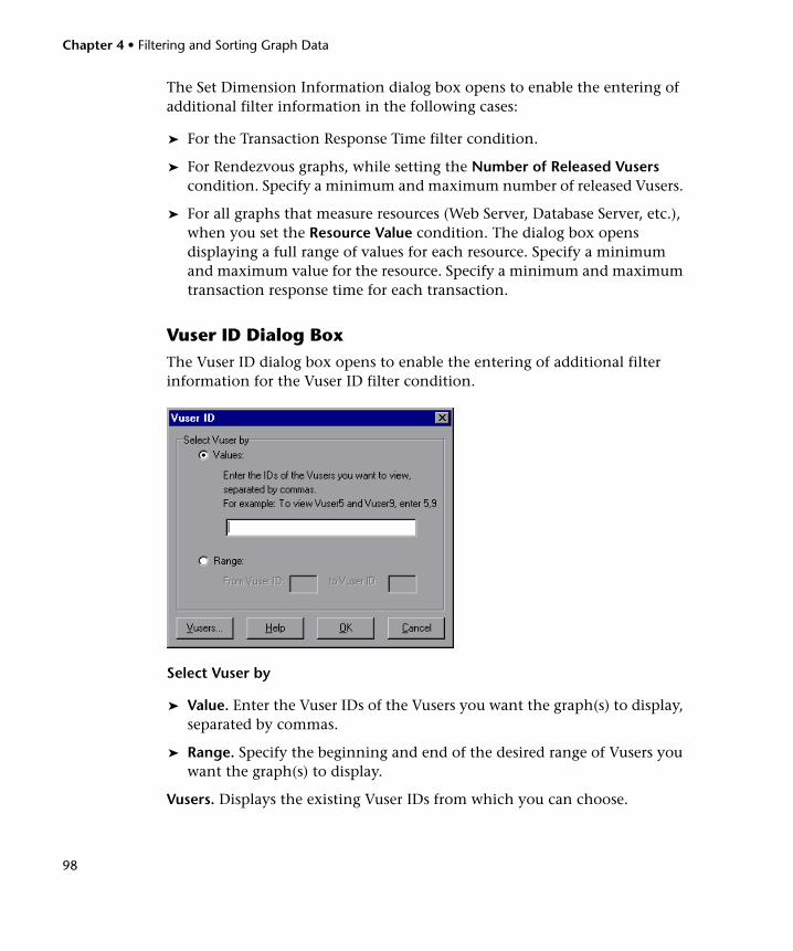
Chapter 4 • Filtering and Sorting Graph Data
98
The Set Dimension Information dialog box opens to enable the entering of additional filter information in the following cases:
➤ For the Transaction Response Time filter condition.
➤ For Rendezvous graphs, while setting the Number of Released Vusers condition. Specify a minimum and maximum number of released Vusers.
➤ For all graphs that measure resources (Web Server, Database Server, etc.), when you set the Resource Value condition. The dialog box opens displaying a full range of values for each resource. Specify a minimum and maximum value for the resource. Specify a minimum and maximum transaction response time for each transaction.
Vuser ID Dialog BoxThe Vuser ID dialog box opens to enable the entering of additional filter information for the Vuser ID filter condition.
Select Vuser by
➤ Value. Enter the Vuser IDs of the Vusers you want the graph(s) to display, separated by commas.
➤ Range. Specify the beginning and end of the desired range of Vusers you want the graph(s) to display.
Vusers. Displays the existing Vuser IDs from which you can choose.
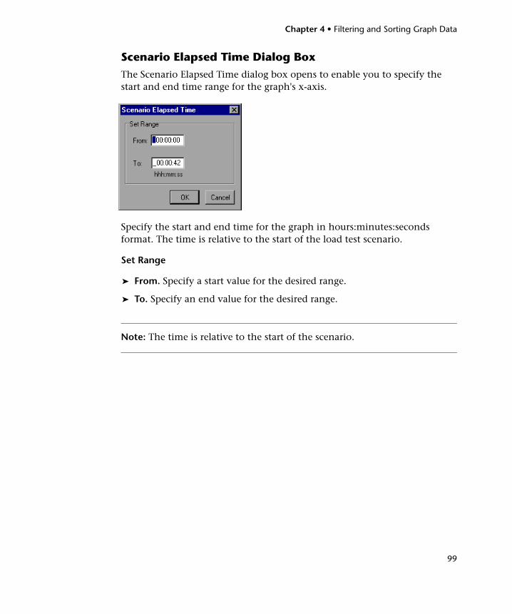
Chapter 4 • Filtering and Sorting Graph Data
99
Scenario Elapsed Time Dialog BoxThe Scenario Elapsed Time dialog box opens to enable you to specify the start and end time range for the graph's x-axis.
Specify the start and end time for the graph in hours:minutes:seconds format. The time is relative to the start of the load test scenario.
Set Range
➤ From. Specify a start value for the desired range.
➤ To. Specify an end value for the desired range.
Note: The time is relative to the start of the scenario.
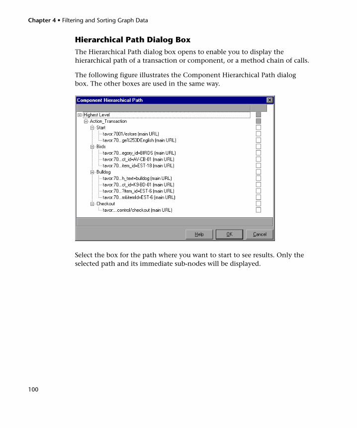
Chapter 4 • Filtering and Sorting Graph Data
100
Hierarchical Path Dialog BoxThe Hierarchical Path dialog box opens to enable you to display the hierarchical path of a transaction or component, or a method chain of calls.
The following figure illustrates the Component Hierarchical Path dialog box. The other boxes are used in the same way.
Select the box for the path where you want to start to see results. Only the selected path and its immediate sub-nodes will be displayed.
101
5Working with Analysis Graph Data
Analysis contains several utilities that enable you to manage graph data to most effectively view the displayed data.
This chapter includes:
➤ Determining a Point’s Coordinates on page 102
➤ Drilling Down in a Graph on page 102
➤ Changing the Granularity of the Data on page 105
➤ Viewing Measurement Trends on page 107
➤ Auto Correlating Measurements on page 108
➤ Viewing Graph Data on page 114
➤ Viewing and Editing Graph Properties on page 117
Note: The graph data is accurate up to the third decimal place.
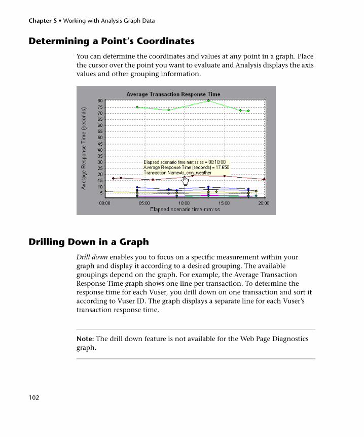
Chapter 5 • Working with Analysis Graph Data
102
Determining a Point’s Coordinates
You can determine the coordinates and values at any point in a graph. Place the cursor over the point you want to evaluate and Analysis displays the axis values and other grouping information.
Drilling Down in a Graph
Drill down enables you to focus on a specific measurement within your graph and display it according to a desired grouping. The available groupings depend on the graph. For example, the Average Transaction Response Time graph shows one line per transaction. To determine the response time for each Vuser, you drill down on one transaction and sort it according to Vuser ID. The graph displays a separate line for each Vuser’s transaction response time.
Note: The drill down feature is not available for the Web Page Diagnostics graph.
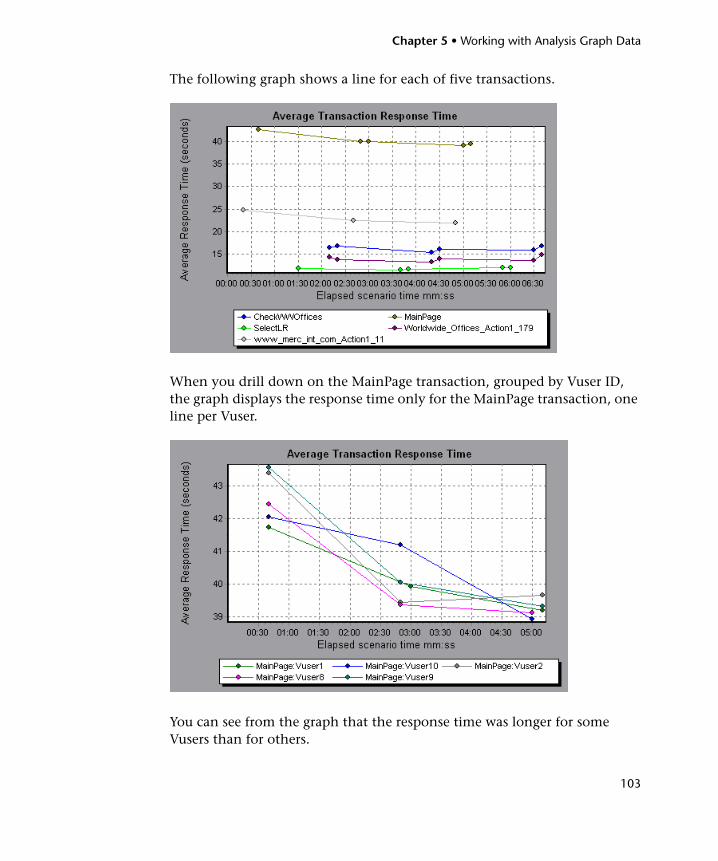
Chapter 5 • Working with Analysis Graph Data
103
The following graph shows a line for each of five transactions.
When you drill down on the MainPage transaction, grouped by Vuser ID, the graph displays the response time only for the MainPage transaction, one line per Vuser.
You can see from the graph that the response time was longer for some Vusers than for others.
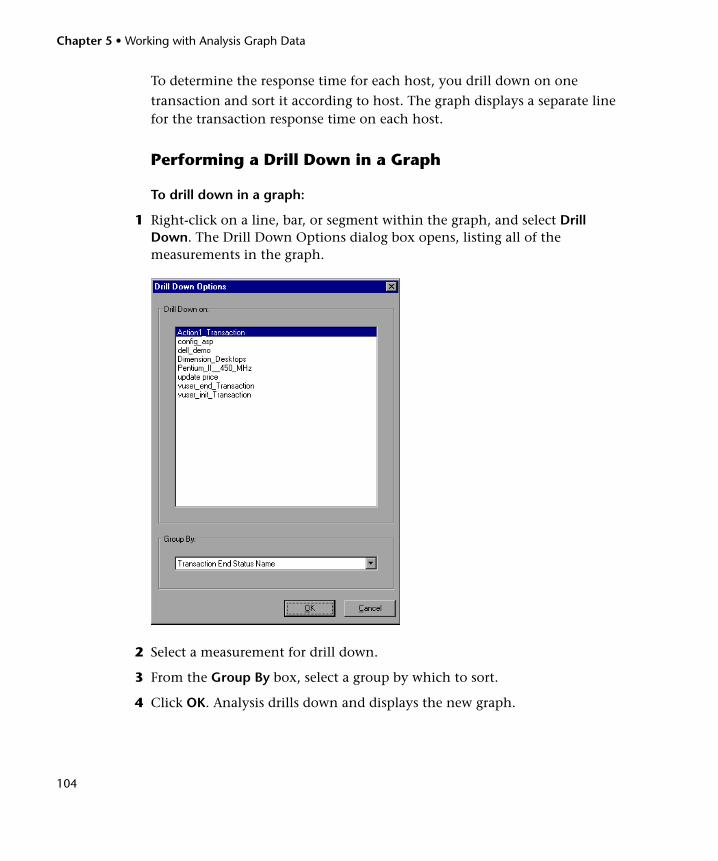
Chapter 5 • Working with Analysis Graph Data
104
To determine the response time for each host, you drill down on one
transaction and sort it according to host. The graph displays a separate line for the transaction response time on each host.
Performing a Drill Down in a Graph
To drill down in a graph:
1 Right-click on a line, bar, or segment within the graph, and select Drill Down. The Drill Down Options dialog box opens, listing all of the measurements in the graph.
2 Select a measurement for drill down.
3 From the Group By box, select a group by which to sort.
4 Click OK. Analysis drills down and displays the new graph.

Chapter 5 • Working with Analysis Graph Data
105
To undo the last drill down settings, choose Undo Set Filter/Group By from the right-click menu.
➤ To perform additional drill downs, repeat steps 1 to 4.
➤ To clear all filter and drill down settings, choose Clear Filter/Group By from the right-click menu.
Changing the Granularity of the Data
You can make the graphs easier to read and analyze by changing the granularity (scale) of the x-axis. The maximum granularity is half of the graph's time range. To ensure readability and clarity, Analysis automatically adjusts the minimum granularity of graphs with ranges of 500 seconds or more.
In the following example, the Hits per Second graph is displayed using different granularities. The y-axis represents the number of hits per second within the granularity interval. For a granularity of 1, the y-axis shows the number of hits per second for each one second period of the load test scenario.
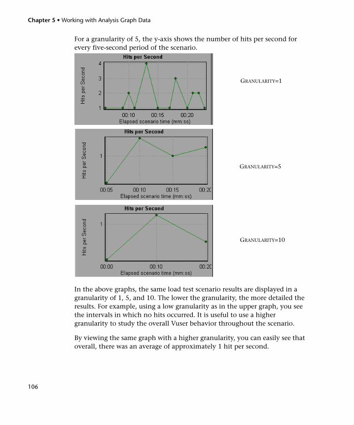
Chapter 5 • Working with Analysis Graph Data
106
For a granularity of 5, the y-axis shows the number of hits per second for every five-second period of the scenario.
In the above graphs, the same load test scenario results are displayed in a granularity of 1, 5, and 10. The lower the granularity, the more detailed the results. For example, using a low granularity as in the upper graph, you see the intervals in which no hits occurred. It is useful to use a higher granularity to study the overall Vuser behavior throughout the scenario.
By viewing the same graph with a higher granularity, you can easily see that overall, there was an average of approximately 1 hit per second.
GRANULARITY=1
GRANULARITY=5
GRANULARITY=10
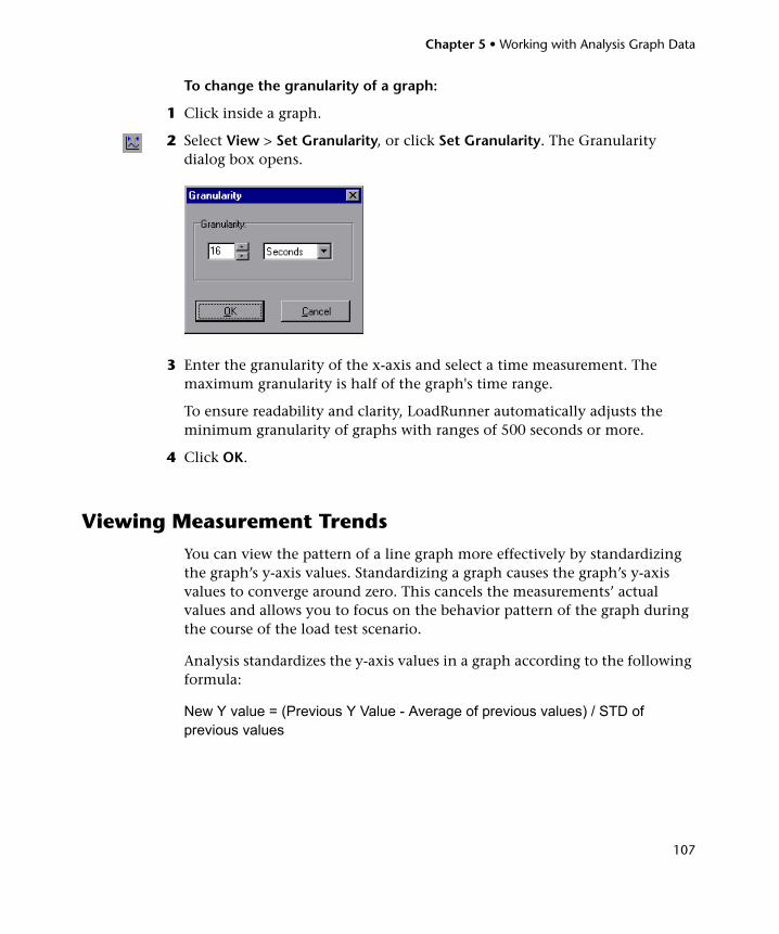
Chapter 5 • Working with Analysis Graph Data
107
To change the granularity of a graph:
1 Click inside a graph.
2 Select View > Set Granularity, or click Set Granularity. The Granularity dialog box opens.
3 Enter the granularity of the x-axis and select a time measurement. The maximum granularity is half of the graph's time range.
To ensure readability and clarity, LoadRunner automatically adjusts the minimum granularity of graphs with ranges of 500 seconds or more.
4 Click OK.
Viewing Measurement Trends
You can view the pattern of a line graph more effectively by standardizing the graph’s y-axis values. Standardizing a graph causes the graph’s y-axis values to converge around zero. This cancels the measurements’ actual values and allows you to focus on the behavior pattern of the graph during the course of the load test scenario.
Analysis standardizes the y-axis values in a graph according to the following formula:
New Y value = (Previous Y Value - Average of previous values) / STD of previous values
Chapter 5 • Working with Analysis Graph Data
108
To view a line graph as a standardized graph:
1 Select View > View Measurement Trends, or right-click the graph and choose View Measurement Trends. Alternatively, you can select View > Configure Measurements and check the View measurement trends for all measurements box.
Note: The standardization feature can be applied to all line graphs except the Web Page Diagnostics graph.
2 View the standardized values for the line graph you selected. The values in the Minimum, Average, Maximum, and Std. Deviation legend columns are real values.
To undo the standardization of a graph, repeat step 1.
Note: If you standardize two line graphs, the two y-axes merge into one y-axis.
Auto Correlating Measurements
You can detect similar trends among measurements by correlating a measurement in one graph with measurements in other graphs. Correlation cancels the measurements’ actual values and allows you to focus on the behavior pattern of the measurements during a specified time range of the load test scenario.
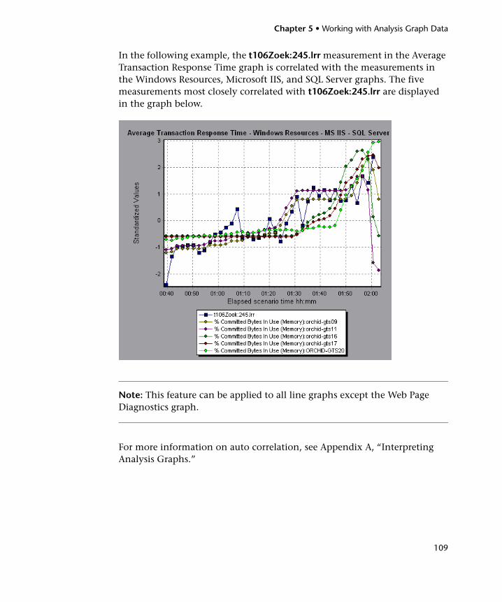
Chapter 5 • Working with Analysis Graph Data
109
In the following example, the t106Zoek:245.lrr measurement in the Average Transaction Response Time graph is correlated with the measurements in the Windows Resources, Microsoft IIS, and SQL Server graphs. The five measurements most closely correlated with t106Zoek:245.lrr are displayed in the graph below.
Note: This feature can be applied to all line graphs except the Web Page Diagnostics graph.
For more information on auto correlation, see Appendix A, “Interpreting Analysis Graphs.”
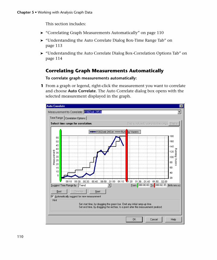
Chapter 5 • Working with Analysis Graph Data
110
This section includes:
➤ “Correlating Graph Measurements Automatically” on page 110
➤ “Understanding the Auto Correlate Dialog Box-Time Range Tab” on page 113
➤ “Understanding the Auto Correlate Dialog Box-Correlation Options Tab” on page 114
Correlating Graph Measurements AutomaticallyTo correlate graph measurements automatically:
1 From a graph or legend, right-click the measurement you want to correlate and choose Auto Correlate. The Auto Correlate dialog box opens with the selected measurement displayed in the graph.
Chapter 5 • Working with Analysis Graph Data
111
The following settings configure the Auto Correlate tool to automatically demarcate the most significant time period for the measurement in the load test scenario. For more information, see “Understanding the Auto Correlate Dialog Box-Time Range Tab” on page 113.
Note: The Running Vusers graph is superimposed on the selected measurement graph only to assist you in selecting an appropriate time range. The left y-axis shows the measurement's values. The right y-axis shows the number of Running Vusers.
2 Select a suggested time range method and time range.
3 If you applied a time filter to your graph, you can correlate values for the complete scenario time range by clicking the Display button in the upper right-hand corner of the dialog box.
Note: The granularity of the correlated measurements graph may differ from that of the original graph, depending on the scenario time range defined.
4 To specify the graphs you want to correlate with a selected measurement and the type of graph output to be displayed, perform the following:
➤ Select the Correlation Options tab.
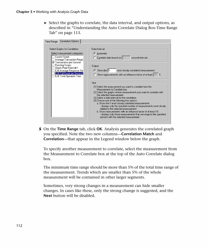
Chapter 5 • Working with Analysis Graph Data
112
➤ Select the graphs to correlate, the data interval, and output options, as described in “Understanding the Auto Correlate Dialog Box-Time Range Tab” on page 113.
5 On the Time Range tab, click OK. Analysis generates the correlated graph you specified. Note the two new columns—Correlation Match and Correlation—that appear in the Legend window below the graph.
To specify another measurement to correlate, select the measurement from the Measurement to Correlate box at the top of the Auto Correlate dialog box.
The minimum time range should be more than 5% of the total time range of the measurement. Trends which are smaller than 5% of the whole measurement will be contained in other larger segments.
Sometimes, very strong changes in a measurement can hide smaller changes. In cases like these, only the strong change is suggested, and the Next button will be disabled.
Chapter 5 • Working with Analysis Graph Data
113
Understanding the Auto Correlate Dialog Box-Time Range Tab
The Time Range tab of the Auto Correlate dialog box enables you to specify a load test scenario time range for the correlated measurement graph.
➤ Measurement to Correlate. Select the measurement you want to correlate.
➤ Display values for complete time range. Click Display to correlate values for the complete scenario time range. This option is available only if you applied a time filter to your graph.
➤ Suggest Time Range By. Analysis automatically demarcates the most significant time period for the measurement in the scenario.
➤ Trend. Demarcates an extended time segment which contains the most significant changes.
➤ Feature. Demarcates a smaller dimension segment which forms the trend.
➤ Best. Choose the time segment most dissimilar to its adjacent segments.
➤ Next. Suggest the next time segment for auto correlation. Each suggestion is successively less dissimilar.
➤ Previous. Return to the previous suggestion of a time segment.
➤ Automatically suggest for new measurement. Generates new suggestions each time that the Measurement to Correlate item changes.
➤ From. Specify a start value (in hh:mm:ss format) for the desired scenario time range.
➤ To. Specify an end value (in hh:mm:ss format) for the desired scenario time range.
You can also use the green and red vertical drag bars to specify the start and end values for the scenario time range.
Note: The granularity of the correlated measurements graph may differ from that of the original graph, depending on the scenario time range defined.
Chapter 5 • Working with Analysis Graph Data
114
Understanding the Auto Correlate Dialog Box-Correlation Options Tab
You use the Correlation Options tab of the Auto Correlate dialog box to set the graphs to correlate, the data interval, and the output options.
➤ Select Graphs for Correlation. Select the graphs whose measurements you want to correlate with your selected measurement.
➤ Data Interval. Calculate the interval between correlation measurement polls.
➤ Automatic. Uses an automatic value, determined by the time range.
➤ Correlate data based on X second intervals. Enter a fixed value.
➤ Output. Choose the level of output displayed.
➤ Show the X most closely correlated measurements. Displays only the specified number of measurements most closely related to the selected measurement. The default setting is 5.
➤ Show measurements with an influence factor of at least X%. Displays only those measurements that converge to the specified percent with the selected measurement. The default setting is 50%.
Viewing Graph Data
Analysis allows you to view graph data in the following ways.
➤ Spreadsheet View. View the graph values displayed in the Graph Data window. (Windows > Graph Data)
➤ Raw Data View. View the actual raw data collected during the load test scenario, displayed in the Raw Data window (Windows > Raw Data).
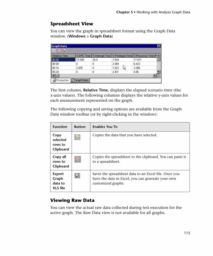
Chapter 5 • Working with Analysis Graph Data
115
Spreadsheet ViewYou can view the graph in spreadsheet format using the Graph Data window. (Windows > Graph Data)
The first column, Relative Time, displays the elapsed scenario time (the x-axis values). The following columns displays the relative y-axis values for each measurement represented on the graph.
The following copying and saving options are available from the Graph Data window toolbar (or by right-clicking in the window):
Viewing Raw DataYou can view the actual raw data collected during test execution for the active graph. The Raw Data view is not available for all graphs.
Function Button Enables You To
Copy selected rows to Clipboard
Copies the data that you have selected.
Copy all rows to Clipboard
Copies the spreadsheet to the clipboard. You can paste it to a spreadsheet.
Export Graph data to XLS file
Saves the spreadsheet data to an Excel file. Once you have the data in Excel, you can generate your own customized graphs.
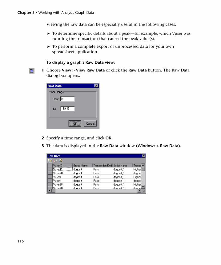
Chapter 5 • Working with Analysis Graph Data
116
Viewing the raw data can be especially useful in the following cases:
➤ To determine specific details about a peak—for example, which Vuser was running the transaction that caused the peak value(s).
➤ To perform a complete export of unprocessed data for your own spreadsheet application.
To display a graph’s Raw Data view:
1 Choose View > View Raw Data or click the Raw Data button. The Raw Data dialog box opens.
2 Specify a time range, and click OK.
3 The data is displayed in the Raw Data window (Windows > Raw Data).
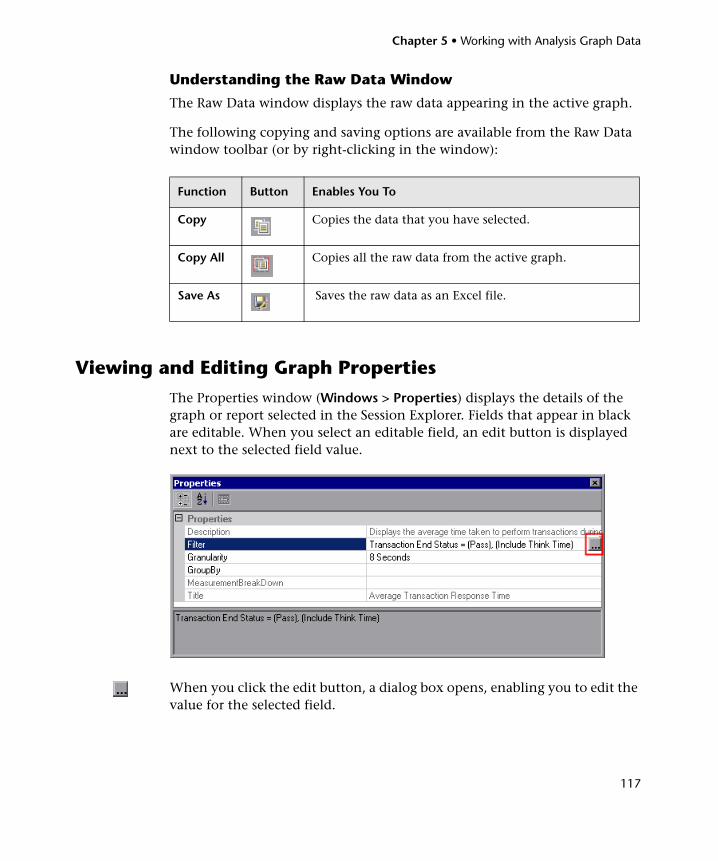
Chapter 5 • Working with Analysis Graph Data
117
Understanding the Raw Data Window
The Raw Data window displays the raw data appearing in the active graph.
The following copying and saving options are available from the Raw Data window toolbar (or by right-clicking in the window):
Viewing and Editing Graph Properties
The Properties window (Windows > Properties) displays the details of the graph or report selected in the Session Explorer. Fields that appear in black are editable. When you select an editable field, an edit button is displayed next to the selected field value.
When you click the edit button, a dialog box opens, enabling you to edit the value for the selected field.
Function Button Enables You To
Copy Copies the data that you have selected.
Copy All Copies all the raw data from the active graph.
Save As Saves the raw data as an Excel file.
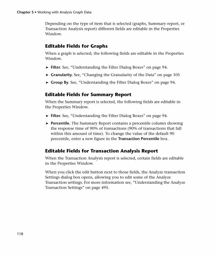
Chapter 5 • Working with Analysis Graph Data
118
Depending on the type of item that is selected (graphs, Summary report, or Transaction Analysis report) different fields are editable in the Properties Window.
Editable Fields for GraphsWhen a graph is selected, the following fields are editable in the Properties Window.
➤ Filter. See, “Understanding the Filter Dialog Boxes” on page 94.
➤ Granularity. See, “Changing the Granularity of the Data” on page 105
➤ Group By. See, “Understanding the Filter Dialog Boxes” on page 94.
Editable Fields for Summary ReportWhen the Summary report is selected, the following fields are editable in the Properties Window.
➤ Filter. See, “Understanding the Filter Dialog Boxes” on page 94.
➤ Percentile. The Summary Report contains a percentile column showing the response time of 90% of transactions (90% of transactions that fall within this amount of time). To change the value of the default 90 percentile, enter a new figure in the Transaction Percentile box.
Editable Fields for Transaction Analysis ReportWhen the Transaction Analysis report is selected, certain fields are editable in the Properties Window.
When you click the edit button next to those fields, the Analyze transaction Settings dialog box opens, allowing you to edit some of the Analyze Transaction settings. For more information see, “Understanding the Analyze Transaction Settings” on page 495.
119
6 Viewing Load Test Scenario Information
In Analysis, you can view information about the load test scenario which you are analyzing. You can view the scenario run time settings and output messages that were generated by the Controller during the scenario.
This chapter includes:
➤ Viewing the Load Test Scenario Run Time Settings on page 119
➤ Viewing Load Test Scenario Output Messages on page 121
Viewing the Load Test Scenario Run Time Settings
You can view information about the Vuser groups and scripts that were run in each scenario, as well as the run time settings for each script in a scenario, in the Scenario Run Time Settings dialog box.
Note: The run time settings allow you to customize the way a Vuser script is executed. You configure the run time settings from the Controller or Virtual User Generator (VuGen) before running a scenario. For information on configuring the run time settings, refer to the HP Virtual User Generator User Guide.
Choose File > View Scenario Run Time Settings, or click View Run Time Settings on the toolbar.
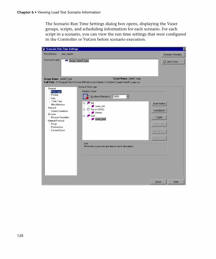
Chapter 6 • Viewing Load Test Scenario Information
120
The Scenario Run Time Settings dialog box opens, displaying the Vuser groups, scripts, and scheduling information for each scenario. For each script in a scenario, you can view the run time settings that were configured in the Controller or VuGen before scenario execution.
Chapter 6 • Viewing Load Test Scenario Information
121
Understanding the Scenario Run Time Settings Dialog BoxThe Scenario Run Time Settings dialog box enables you to view information about executed load test scenarios, as well as the run time settings for each script in a scenario.
➤ Result Name. The name of the result file.
➤ Scenario Scripts. Displays the result set for each executed scenario, as well as the Vuser groups and scripts that were run in the scenario.
➤ Group Name. Displays the name of the group to which the selected script belongs.
➤ Full Path. Displays the script’s full directory path.
➤ Script Name. Displays the name of the selected script.
➤ Scenario Schedule. Displays goal-oriented or manual scenario scheduling information for the selected scenario.
➤ View Script. Opens the Virtual User Generator, so that you can edit the script. For more information on editing scripts, refer to the HP Virtual User Generator User Guide.
The options in the lower half of the screen are described in full in the HP Virtual User Generator User Guide.
Viewing Load Test Scenario Output Messages
When the load test scenario runs, the Vusers and load generators send error, notification, warning, debug, and batch messages to the Controller.
In Analysis, you can view these output messages in the Controller Output Messages window (Windows > Controller Output Messages).
This section includes:
➤ “Configuring Controller Output Messages Settings” on page 122
➤ “Viewing messages in the Controller Output Messages window” on page 123
➤ “Viewing Log Information Details” on page 124
➤ “Understanding the Controller Output Messages Window” on page 124
Chapter 6 • Viewing Load Test Scenario Information
122
Configuring Controller Output Messages SettingsWhen you choose to display Controller output messages in Analysis, Analysis searches for the output data in the current Analysis session. If the data is not found, it searches in the scenario results directory. If Analysis cannot locate the results directory, no messages are displayed.
You can choose to copy the output messages generated by the Controller to the Analysis session so that this data is always available to Analysis, even if the scenario results directory cannot be located.
To copy Controller output messages to the Analysis session:
1 Choose Tools > Options and select the Result Collection tab.
2 In the Copy Controller Output Messages to Analysis Session area, choose one of the following options:
➤ Copy if data set is smaller than X MB. Copies the Controller output data to the Analysis session if the data set is smaller than the amount you specify.
➤ Always Copy. Always copies the Controller output data to the Analysis session.
➤ Never Copy. Never copies the Controller output data to the Analysis session.
3 Apply your settings.
➤ To apply these settings to the current session, click Apply now to active session.
➤ To apply these settings after the current session is saved, click OK.
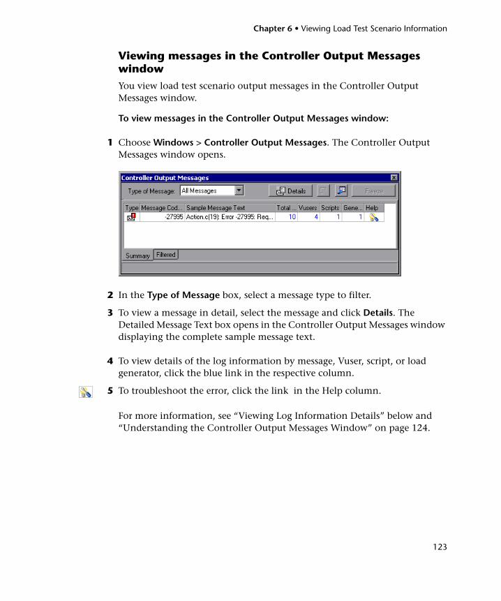
Chapter 6 • Viewing Load Test Scenario Information
123
Viewing messages in the Controller Output Messages windowYou view load test scenario output messages in the Controller Output Messages window.
To view messages in the Controller Output Messages window:
1 Choose Windows > Controller Output Messages. The Controller Output Messages window opens.
2 In the Type of Message box, select a message type to filter.
3 To view a message in detail, select the message and click Details. The Detailed Message Text box opens in the Controller Output Messages window displaying the complete sample message text.
4 To view details of the log information by message, Vuser, script, or load generator, click the blue link in the respective column.
5 To troubleshoot the error, click the link in the Help column.
For more information, see “Viewing Log Information Details” below and “Understanding the Controller Output Messages Window” on page 124.
Chapter 6 • Viewing Load Test Scenario Information
124
Viewing Log Information Details
You can view details of each message, Vuser, script, and load generator associated with an error code by clicking the blue link in the respective column. The Controller Output Messages window displays a drilled-down view by Vuser, message, script, or load generator in the Filtered tab.
For example, if you drill down on the Vusers column, the Controller Output Messages window displays all the messages with the code you selected, grouped by the Vusers that sent the messages.
The message type, the message code, and the column that you selected to drill down on, are displayed above the grid.
You can drill down further on the entries displayed in blue. When you drill down on a Vuser, the Vuser log opens.
To move between the various drill down levels, click the Previous view and Next view buttons in the upper-left corner of the Controller Output Messages window.
Understanding the Controller Output Messages WindowThe Controller Output Messages window displays information about the error, notification, warning, debug, and batch messages that Vusers and load generators send to the Controller during scenario execution.
Summary Tab
The Summary tab displays summary information about the messages sent during scenario execution. To view details of each message, Vuser, script, and load generator associated with an error code, click the blue link in the respective column.
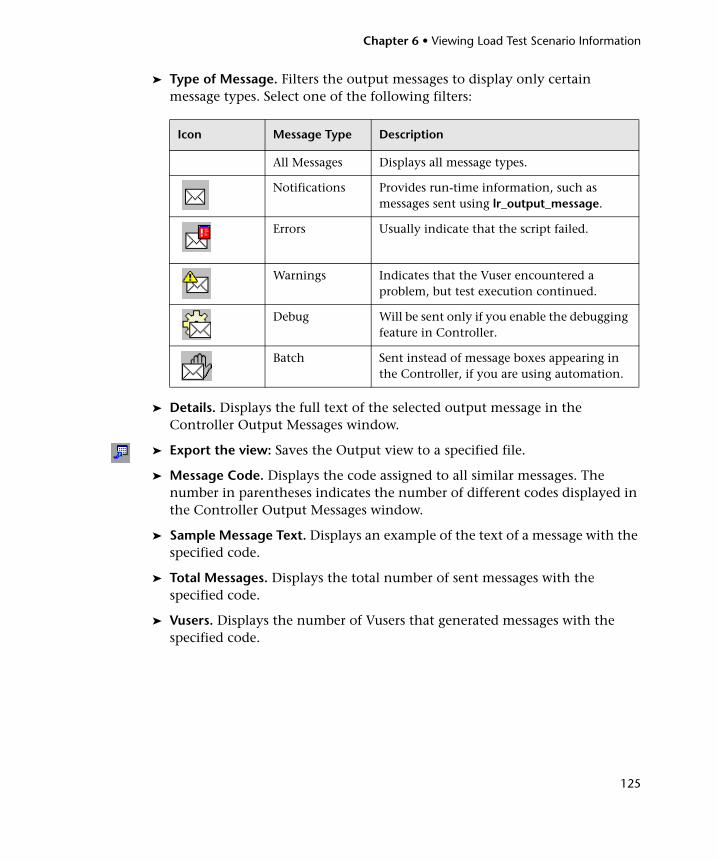
Chapter 6 • Viewing Load Test Scenario Information
125
➤ Type of Message. Filters the output messages to display only certain message types. Select one of the following filters:
➤ Details. Displays the full text of the selected output message in the Controller Output Messages window.
➤ Export the view: Saves the Output view to a specified file.
➤ Message Code. Displays the code assigned to all similar messages. The number in parentheses indicates the number of different codes displayed in the Controller Output Messages window.
➤ Sample Message Text. Displays an example of the text of a message with the specified code.
➤ Total Messages. Displays the total number of sent messages with the specified code.
➤ Vusers. Displays the number of Vusers that generated messages with the specified code.
Icon Message Type Description
All Messages Displays all message types.
Notifications Provides run-time information, such as messages sent using lr_output_message.
Errors Usually indicate that the script failed.
Warnings Indicates that the Vuser encountered a problem, but test execution continued.
Debug Will be sent only if you enable the debugging feature in Controller.
Batch Sent instead of message boxes appearing in the Controller, if you are using automation.
Chapter 6 • Viewing Load Test Scenario Information
126
➤ Scripts. Displays the number of scripts whose execution caused messages with the specified code to be generated.
➤ Generators. Displays the number of load generators from which messages with the specified code were generated.
➤ Help. Displays an icon if there is a link to troubleshooting for this message.
Note: To sort the log information, click the appropriate column header. The messages are sorted in descending/ascending order.
Filtered Tab
The Filtered tab displays a drilled down view by Vuser, message, script, or load generator. For example, if you drill down on the Vusers column, the Filtered tab displays all the messages with the code you selected, grouped by the Vusers that sent the messages.
➤ Previous view/Next view. Enables you to move between the various drill down levels.
➤ <Type of Message> Icon. Displays an icon indicating the type of message by which the current Output view is filtered.
➤ Active Filter. Displays the category or categories by which the current Output view is filtered.
➤ Viewed by. Displays the name of the column on which you selected to drill down.
➤ Export the view. Saves the Output view to a specified file.

127
7 Cross Result and Merged Graphs
The Analysis utility lets you compare results and graphs to determine the source of a problem.
This chapter includes:
➤ About Cross Result and Merged Graphs on page 127
➤ Cross Result Graphs on page 128
➤ Generating Cross Result Graphs on page 130
➤ Merging Graphs on page 131
About Cross Result and Merged Graphs
Comparing results is essential for determining bottlenecks and problems. You use Cross Result graphs to compare the results of multiple load test scenario runs. You create Merged graphs to compare results from different graphs within the same scenario run.
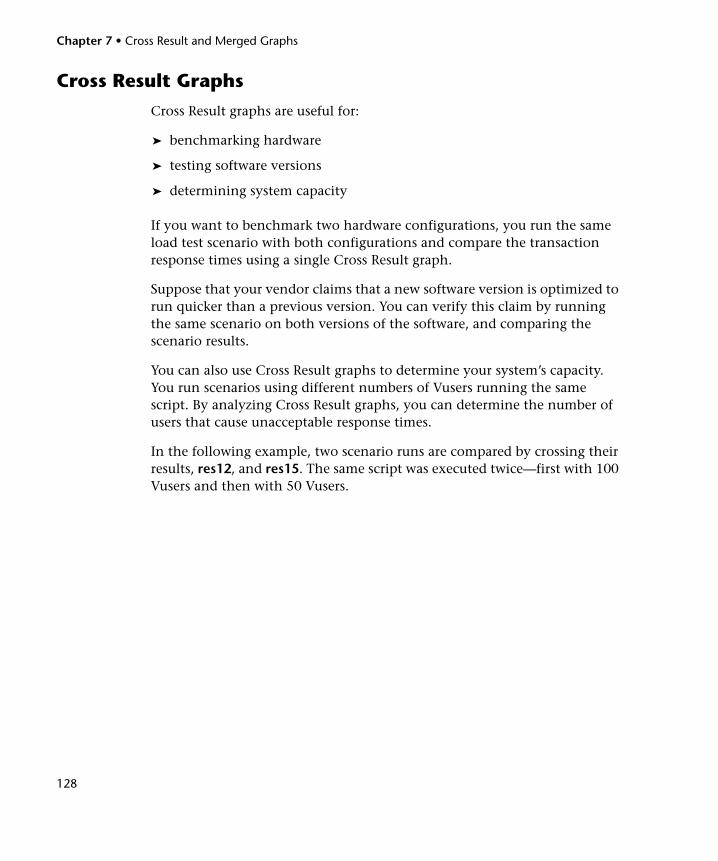
Chapter 7 • Cross Result and Merged Graphs
128
Cross Result Graphs
Cross Result graphs are useful for:
➤ benchmarking hardware
➤ testing software versions
➤ determining system capacity
If you want to benchmark two hardware configurations, you run the same load test scenario with both configurations and compare the transaction response times using a single Cross Result graph.
Suppose that your vendor claims that a new software version is optimized to run quicker than a previous version. You can verify this claim by running the same scenario on both versions of the software, and comparing the scenario results.
You can also use Cross Result graphs to determine your system’s capacity. You run scenarios using different numbers of Vusers running the same script. By analyzing Cross Result graphs, you can determine the number of users that cause unacceptable response times.
In the following example, two scenario runs are compared by crossing their results, res12, and res15. The same script was executed twice—first with 100 Vusers and then with 50 Vusers.
Chapter 7 • Cross Result and Merged Graphs
129
In the first run, the average transaction time was approximately 59 seconds. In the second run, the average time was 4.7 seconds. It is apparent that the system works much slower with a greater load.
The Cross Result graphs have an additional filter and group by category: Result Name. The above graph is filtered to the OrderRide transaction for results res12, and res15, grouped by Result Name.
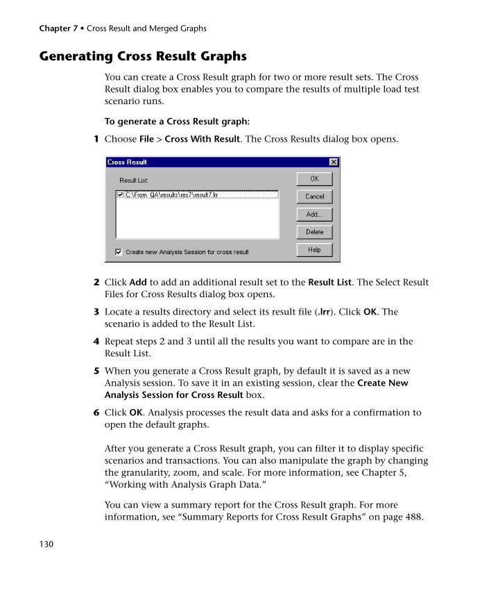
Chapter 7 • Cross Result and Merged Graphs
130
Generating Cross Result Graphs
You can create a Cross Result graph for two or more result sets. The Cross Result dialog box enables you to compare the results of multiple load test scenario runs.
To generate a Cross Result graph:
1 Choose File > Cross With Result. The Cross Results dialog box opens.
2 Click Add to add an additional result set to the Result List. The Select Result Files for Cross Results dialog box opens.
3 Locate a results directory and select its result file (.lrr). Click OK. The scenario is added to the Result List.
4 Repeat steps 2 and 3 until all the results you want to compare are in the Result List.
5 When you generate a Cross Result graph, by default it is saved as a new Analysis session. To save it in an existing session, clear the Create New Analysis Session for Cross Result box.
6 Click OK. Analysis processes the result data and asks for a confirmation to open the default graphs.
After you generate a Cross Result graph, you can filter it to display specific scenarios and transactions. You can also manipulate the graph by changing the granularity, zoom, and scale. For more information, see Chapter 5, “Working with Analysis Graph Data.”
You can view a summary report for the Cross Result graph. For more information, see “Summary Reports for Cross Result Graphs” on page 488.
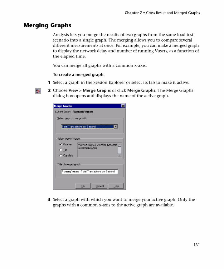
Chapter 7 • Cross Result and Merged Graphs
131
Merging Graphs
Analysis lets you merge the results of two graphs from the same load test scenario into a single graph. The merging allows you to compare several different measurements at once. For example, you can make a merged graph to display the network delay and number of running Vusers, as a function of the elapsed time.
You can merge all graphs with a common x-axis.
To create a merged graph:
1 Select a graph in the Session Explorer or select its tab to make it active.
2 Choose View > Merge Graphs or click Merge Graphs. The Merge Graphs dialog box opens and displays the name of the active graph.
3 Select a graph with which you want to merge your active graph. Only the graphs with a common x-axis to the active graph are available.
Chapter 7 • Cross Result and Merged Graphs
132
4 Select the merge type and a title for the merged graph. By default, Analysis combines the titles of the two graphs being merged. For more information, see “Understanding the Merge Graphs Dialog Box” on page 132.
5 Click OK.
6 Filter the graph just as you would filter any ordinary graph.
Understanding the Merge Graphs Dialog BoxThe Merge Graphs dialog box enables you to merge two graphs into a single graph. In order to merge graphs, the graphs' x-axes must be the same measurement. For example, you can merge Web Throughput and Hits per Second graphs, because their x-axes are Scenario Elapsed Time.
Analysis provides three types of merging:
➤ Overlay
➤ Tile
➤ Correlate
Overlay. Superimpose the contents of two graphs that share a common x- axis. The left y-axis on the merged graph shows the current graph's values. The right y-axis shows the values of the graph that was merged. There is no limit to the number of graphs that you can overlay. When you overlay two graphs, the y-axis for each graph is displayed separately to the right and left of the graph. When you overlay more than two graphs, Analysis displays a single y-axis, scaling the different measurements accordingly.
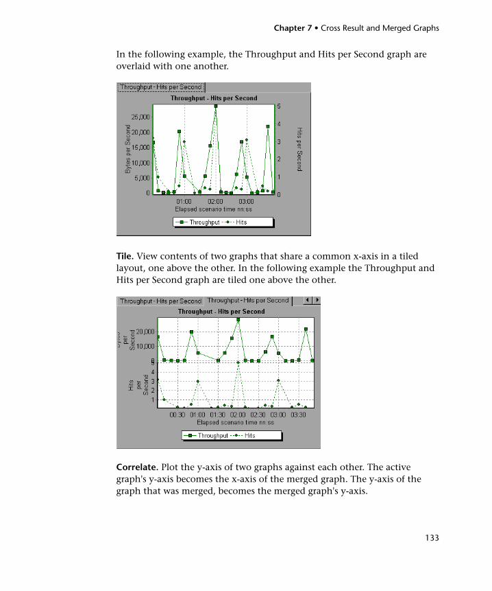
Chapter 7 • Cross Result and Merged Graphs
133
In the following example, the Throughput and Hits per Second graph are overlaid with one another.
Tile. View contents of two graphs that share a common x-axis in a tiled layout, one above the other. In the following example the Throughput and Hits per Second graph are tiled one above the other.
Correlate. Plot the y-axis of two graphs against each other. The active graph's y-axis becomes the x-axis of the merged graph. The y-axis of the graph that was merged, becomes the merged graph's y-axis.
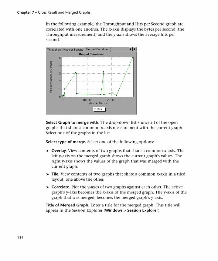
Chapter 7 • Cross Result and Merged Graphs
134
In the following example, the Throughput and Hits per Second graph are correlated with one another. The x-axis displays the bytes per second (the Throughput measurement) and the y-axis shows the average hits per second.
Select Graph to merge with. The drop-down list shows all of the open graphs that share a common x-axis measurement with the current graph. Select one of the graphs in the list.
Select type of merge. Select one of the following options:
➤ Overlay. View contents of two graphs that share a common x-axis. The left y-axis on the merged graph shows the current graph's values. The right y-axis shows the values of the graph that was merged with the current graph.
➤ Tile. View contents of two graphs that share a common x-axis in a tiled layout, one above the other.
➤ Correlate. Plot the y-axes of two graphs against each other. The active graph's y-axis becomes the x-axis of the merged graph. The y-axis of the graph that was merged, becomes the merged graph's y-axis.
Title of Merged Graph. Enter a title for the merged graph. This title will appear in the Session Explorer (Windows > Session Explorer).
135
8Defining Service Level Agreements
Service level agreements (SLAs) enable you to define goals for your load test scenario. During a scenario run, the Controller measures the performance and collects data. Analysis compares this data against thresholds defined in the SLAs.
This chapter includes:
➤ About Defining Service Level Agreements on page 136
➤ Defining an SLA Goal Measured Per Time Interval on page 137
➤ Defining an SLA Goal Measured Over the Whole Run on page 145
➤ Understanding the Service Level Agreement Dialog Box on page 147

Chapter 8 • Defining Service Level Agreements
136
About Defining Service Level Agreements
When you design a load test scenario, you can define goals or service level agreements (SLAs) for the performance metrics. When you run the scenario, LoadRunner gathers and stores performance-related data. When you analyze the run, Analysis compares this data against the SLAs and determines SLA statuses for the defined measurements.
Depending on the measurements that you are evaluating, LoadRunner determines SLA statuses in one of the following ways:
➤ SLA status determined at time intervals over a timeline. Analysis displays SLA statuses at set time intervals—for example, every 10 seconds—over a timeline within the run. For more information, see “Defining an SLA Goal Measured Per Time Interval” on page 137.
➤ SLA status determined over the whole run. Analysis displays a single SLA status for the whole scenario run. For more information, see “Defining an SLA Goal Measured Over the Whole Run” on page 145.
Note: You can define and edit SLAs in the Controller or in Analysis.
For details about viewing SLA information in Analysis reports, see Chapter 31, “Understanding Analysis Reports.”
Chapter 8 • Defining Service Level Agreements
137
Defining an SLA Goal Measured Per Time Interval
For the Average Transaction Response Time and Errors per Second measurements, Analysis displays SLA statuses at set time intervals over a timeline within the run.
That is, at each time interval in the timeline—for example, every 10 seconds—Analysis checks to see if the measurement’s performance has deviated from the threshold defined in the SLA.
When creating SLAs for these measurements, you can also specify load criteria to take into account when comparing the data.
➤ To define SLAs for Average Transaction Response Time, see “SLAs for Average Transaction Response Time” below.
➤ To define SLAs for Errors per Second, see “SLAs for Errors Per Second” on page 141.
➤ To set the time intervals which Analysis uses for evaluating the SLA, see “Selecting a Tracking Period” on page 144.
SLAs for Average Transaction Response TimeThis section explains how to define an SLA for evaluating the status of Average Transaction Response Time during the run. For Average Transaction Response Time, LoadRunner evaluates SLA statuses at set time intervals within the run.
Note: To set the time intervals that Analysis uses for evaluating the SLA, see “Selecting a Tracking Period” on page 144.
To define an SLA for Average Transaction Response Time:
1 Open the Service Level Agreement Wizard.
➤ If you are working in Analysis: Select Tools > Configure SLA Rules to open the Service Level Agreement dialog box. Click New.
Chapter 8 • Defining Service Level Agreements
138
➤ If you are working in the Controller: In the Design tab, in the Service Level Agreement pane, click New.
The Service Level Agreement wizard opens.
2 Complete the SLA Wizard steps, as described in the following sections.
Measurement—Select a Measurement for Your Goal
For Average Transaction Response Time, LoadRunner evaluates SLA statuses at set time intervals within the run.
Under SLA status determined per time intervals over a timeline, select Average Transaction Response Time.
Transactions—Select Transactions
From the Available Transactions list, select the transactions that you want to evaluate as part of your SLA and click Add.
Note: You can select multiple transactions using the CTRL key.
The transactions you selected are displayed in the Selected Transactions list.
Load Criteria—Set Load Criteria
Select load criteria for your goal and define appropriate load value ranges.
Note: In the next wizard step (Thresholds page), you will set different thresholds per each of these load value ranges.
➤ In the Load Criteria box, select the relevant load criteria that you want to use—for example, Running Vusers.
To define an SLA without load criteria, select None in the Load Criteria box.
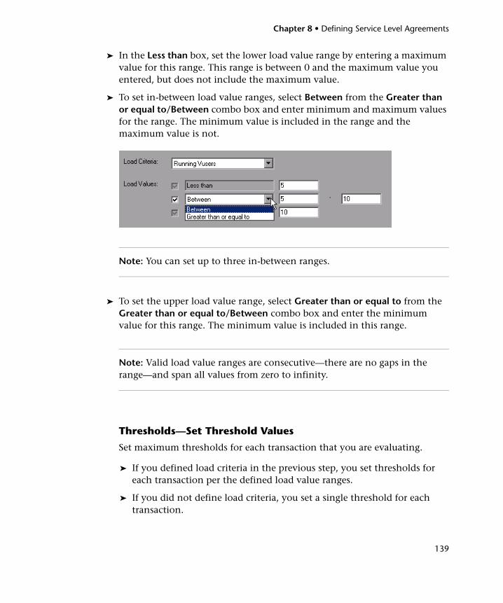
Chapter 8 • Defining Service Level Agreements
139
➤ In the Less than box, set the lower load value range by entering a maximum value for this range. This range is between 0 and the maximum value you entered, but does not include the maximum value.
➤ To set in-between load value ranges, select Between from the Greater than or equal to/Between combo box and enter minimum and maximum values for the range. The minimum value is included in the range and the maximum value is not.
Note: You can set up to three in-between ranges.
➤ To set the upper load value range, select Greater than or equal to from the Greater than or equal to/Between combo box and enter the minimum value for this range. The minimum value is included in this range.
Note: Valid load value ranges are consecutive—there are no gaps in the range—and span all values from zero to infinity.
Thresholds—Set Threshold Values
Set maximum thresholds for each transaction that you are evaluating.
➤ If you defined load criteria in the previous step, you set thresholds for each transaction per the defined load value ranges.
➤ If you did not define load criteria, you set a single threshold for each transaction.
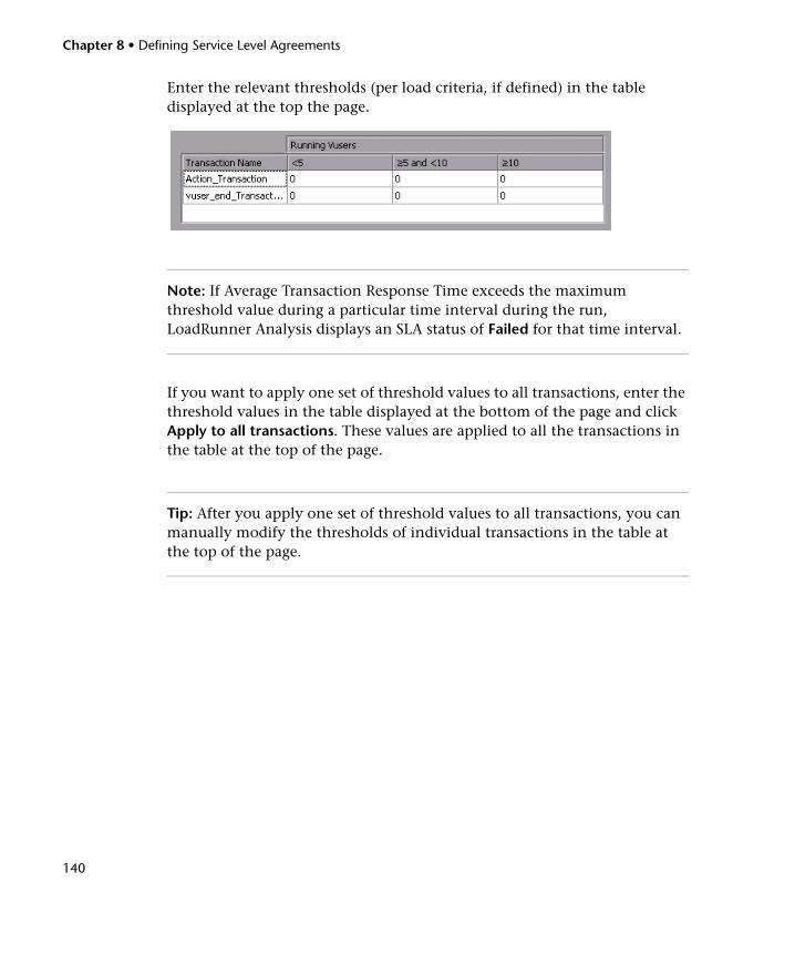
Chapter 8 • Defining Service Level Agreements
140
Enter the relevant thresholds (per load criteria, if defined) in the table displayed at the top the page.
Note: If Average Transaction Response Time exceeds the maximum threshold value during a particular time interval during the run, LoadRunner Analysis displays an SLA status of Failed for that time interval.
If you want to apply one set of threshold values to all transactions, enter the threshold values in the table displayed at the bottom of the page and click Apply to all transactions. These values are applied to all the transactions in the table at the top of the page.
Tip: After you apply one set of threshold values to all transactions, you can manually modify the thresholds of individual transactions in the table at the top of the page.
Chapter 8 • Defining Service Level Agreements
141
Finish
If you want to define another SLA after you save the current one, select Define another SLA.
Click Finish to save the SLA.
In Analysis, when you click Close in the Service Level Agreement dialog box, the Analysis reports are updated with these new SLA definitions.
Note: For details about viewing SLA information in Analysis reports, see Chapter 31, “Understanding Analysis Reports”.
SLAs for Errors Per SecondThis section explains how to define an SLA for evaluating the status of Errors per Second during the run. For Errors per Second, LoadRunner evaluates SLA statuses at set time intervals within the run.
Note: To set the time intervals that Analysis uses for evaluating the SLA, see “Selecting a Tracking Period” on page 144.
To define an SLA for Errors per Second:
1 Open the Service Level Agreement Wizard.
➤ If you are working in Analysis: Select Tools > Configure SLA Rules to open the Service Level Agreement dialog box. Click New.
➤ If you are working in the Controller: In the Design tab, in the Service Level Agreement pane, click New.
The Service Level Agreement wizard opens.
2 Complete the SLA Wizard steps, as described in the following sections.
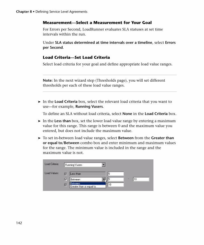
Chapter 8 • Defining Service Level Agreements
142
Measurement—Select a Measurement for Your Goal
For Errors per Second, LoadRunner evaluates SLA statuses at set time intervals within the run.
Under SLA status determined at time intervals over a timeline, select Errors per Second.
Load Criteria—Set Load Criteria
Select load criteria for your goal and define appropriate load value ranges.
Note: In the next wizard step (Thresholds page), you will set different thresholds per each of these load value ranges.
➤ In the Load Criteria box, select the relevant load criteria that you want to use—for example, Running Vusers.
To define an SLA without load criteria, select None in the Load Criteria box.
➤ In the Less than box, set the lower load value range by entering a maximum value for this range. This range is between 0 and the maximum value you entered, but does not include the maximum value.
➤ To set in-between load value ranges, select Between from the Greater than or equal to/Between combo box and enter minimum and maximum values for the range. The minimum value is included in the range and the maximum value is not.
Chapter 8 • Defining Service Level Agreements
143
Note: You can set up to three in-between ranges.
➤ To set the upper load value range, select Greater than or equal to from the Greater than or equal to/Between combo box and enter the minimum value for this range. The minimum value is included in this range.
Note: Valid load value ranges are consecutive—there are no gaps in the range—and span all values from zero to infinity.
Thresholds—Set Threshold Values
In the Thresholds page you set a maximum threshold value for Errors per Second.
➤ If you defined load criteria in the previous step, enter threshold values per the defined load value ranges, in the table provided.
➤ If you did not define load criteria, enter the maximum threshold value in the Threshold box.
Note: If Errors per Second exceeded the maximum threshold value during a particular time interval during the run, LoadRunner Analysis displays an SLA status of Failed for that time interval.
Chapter 8 • Defining Service Level Agreements
144
Finish
If you want to define another SLA after you save the current one, select Define another SLA.
Click Finish to save the SLA.
In Analysis, when you click Close in the Service Level Agreement dialog box, the Analysis reports are updated with these new SLA definitions.
Note: For details about viewing SLA information in Analysis reports, see Chapter 31, “Understanding Analysis Reports”.
Selecting a Tracking PeriodWhen you define a service level agreement for measurements that are evaluated over a timeline, LoadRunner determines SLA statuses at specified time intervals within that timeline. These time intervals are known as the tracking period of the load test scenario.
To define the tracking period for the scenario:
1 In the Design tab, in the Service Level Agreement pane, click the Advanced button. The Advanced Options window opens.
2 Select one of the following methods to determine the tracking period for the scenario.
➤ Internally calculated tracking period.
Analysis sets the tracking period to the minimum value possible, taking into account the aggregation granularity defined for the scenario. This value is at least 5 seconds. It uses the following formula:
➤ Tracking period of at least X seconds.
Select a value (X) to determine the minimum amount of time for the tracking period. This value can never be less than 5 seconds.
Tracking Period = Max (5 seconds, aggregation granularity)
Chapter 8 • Defining Service Level Agreements
145
Analysis sets the tracking period to the nearest multiple of the scenario’s aggregation granularity that is greater than or equal to the value (X) that you selected.
Assume for example that you select a tracking period of X=10, and assume that the aggregation granularity for the scenario is 6. The tracking period is set to the nearest multiple of 6 that is greater than or equal to 10, that is, Tracking Period = 12.
For this option, Analysis uses the following formula:
3 Click OK.
Defining an SLA Goal Measured Over the Whole Run
For certain measurements—Total Hits, Average Hits, Total Throughput, and Average Throughput—Analysis displays a single SLA status for the whole load test scenario run. This section explains how to define an SLA for these measurements.
To define an SLA that evaluates the status over a whole run:
1 Open the Service Level Agreement Wizard.
➤ If you are working in Analysis: Select Tools > Configure SLA Rules to open the Service Level Agreement dialog box. Click New.
➤ If you are working in the Controller: In the Design tab, in the Service Level Agreement pane, click New.
The Service Level Agreement wizard opens.
2 Complete the SLA Wizard steps, as described in the following sections.
Tracking Period = Max(5 seconds, m(Aggregation Granularity))
where m is a multiple of the scenario’s aggregation granularity such that m(Aggregation Granularity) ≥ X
Chapter 8 • Defining Service Level Agreements
146
Measurement—Select a Measurement for Your Goal
For the following measurements, Analysis displays a single SLA status for the whole scenario run:
➤ Total Hits per run
➤ Average Hits (hits/second) per run
➤ Total Throughput (bytes) per run
➤ Average Throughput (bytes/second) per run
Under SLA status determined over the whole run, select the relevant measurement.
Thresholds—Set Threshold Values
The measurement that you selected in the previous step is displayed in the Measurement box.
In the Threshold box, enter the minimum threshold value for your measurement.
Note: If the measurement value fell below this minimum threshold value during the run, LoadRunner Analysis displays an SLA status of Failed for the entire run.
Chapter 8 • Defining Service Level Agreements
147
Finish
If you want to define another SLA after you save the current one, select Define another SLA.
Click Finish to save the SLA.
In Analysis, when you click Close in the Service Level Agreement dialog box, the Analysis reports are updated with these new SLA definitions.
Note: For details about viewing SLA information in Analysis reports, see Chapter 31, “Understanding Analysis Reports”.
Understanding the Service Level Agreement Dialog Box
The Service Level Agreement dialog box includes the following options:
Function Button Enables You To
New Define a new SLA. See:
➤ “Defining an SLA Goal Measured Per Time Interval” on page 137
➤ “Defining an SLA Goal Measured Over the Whole Run” on page 145
Details View the details of the SLA selected in the Service Level Agreement dialog box. The Service Level Agreement - details dialog box opens, displaying a summary of the details for the selected SLA. For more information, see “Understanding the Service Level Agreement - Details Dialog Box” on page 148.
Edit Edit the definitions of the SLA selected in the Service Level Agreement dialog box. The SLA wizard opens with the details of the selected SLA.
Chapter 8 • Defining Service Level Agreements
148
Understanding the Service Level Agreement - Details Dialog BoxThe Service Level Agreement - Details dialog box displays the thresholds that were set for the selected SLA.
If you defined load criteria as part of your SLA, the threshold values are displayed per the defined load value ranges.
For information about defining a new SLA, see About Defining Service Level Agreements.
Delete Delete the SLA selected in the Service Level Agreement dialog box.
Advanced Adjust the tracking period for SLAs that are evaluated per time interval over a timeline. See “Selecting a Tracking Period” on page 144.
Function Button Enables You To
149
9 Managing Results Using Quality Center
LoadRunner’s integration with Quality Center lets you manage Analysis result sessions using Quality Center, HP’s test management tool.
This chapter includes:
➤ About Managing Results Using Quality Center on page 149
➤ Connecting to and Disconnecting from Quality Center on page 150
➤ Opening or Creating a Session Using Quality Center on page 154
➤ Saving Sessions to a Quality Center Project on page 156
About Managing Results Using Quality Center
Analysis works together with Quality Center, HP’s Web-based test management tool. HP Quality Center provides an efficient method for storing and retrieving Vuser scripts, scenarios, and results. You store sessions in a Quality Center project and organize them into unique groups.
In order for Analysis to access a Quality Center project, you must connect it to the Web server on which Quality Center is installed. You can connect to either a local or remote Web server.
For more information on working with Quality Center, see the Quality Center User Guide.
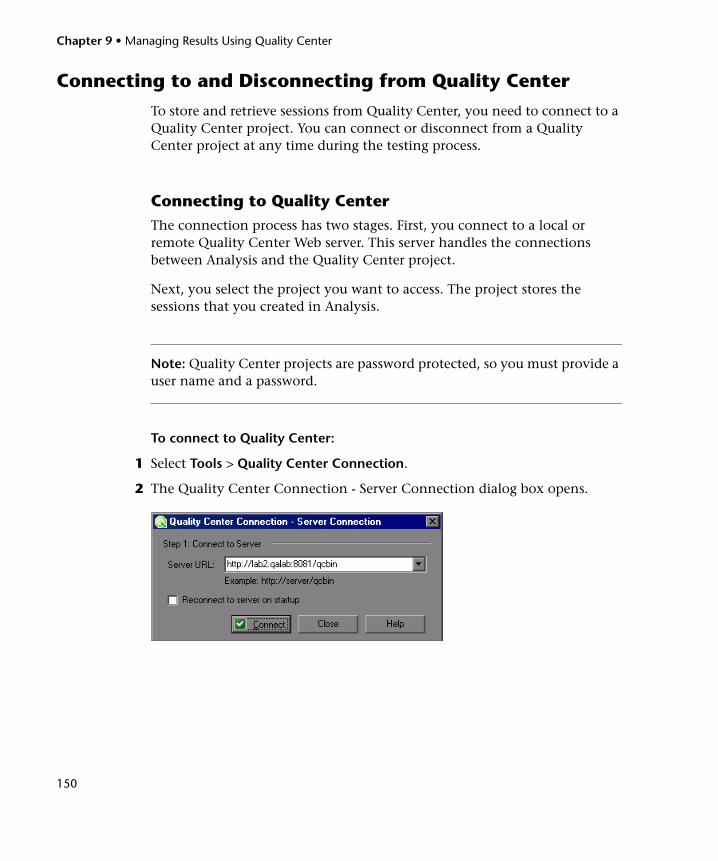
Chapter 9 • Managing Results Using Quality Center
150
Connecting to and Disconnecting from Quality Center
To store and retrieve sessions from Quality Center, you need to connect to a Quality Center project. You can connect or disconnect from a Quality Center project at any time during the testing process.
Connecting to Quality CenterThe connection process has two stages. First, you connect to a local or remote Quality Center Web server. This server handles the connections between Analysis and the Quality Center project.
Next, you select the project you want to access. The project stores the sessions that you created in Analysis.
Note: Quality Center projects are password protected, so you must provide a user name and a password.
To connect to Quality Center:
1 Select Tools > Quality Center Connection.
2 The Quality Center Connection - Server Connection dialog box opens.
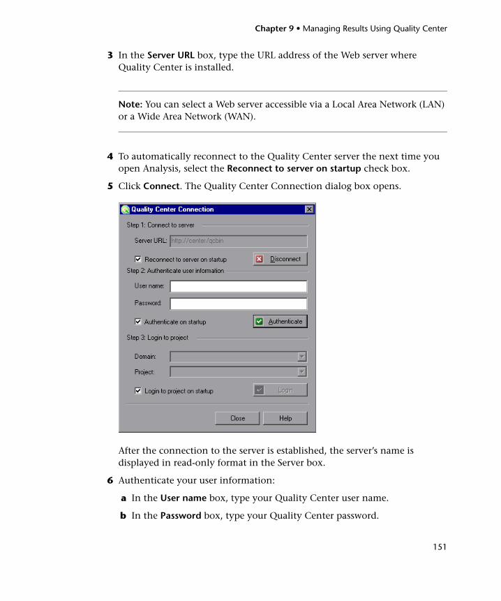
Chapter 9 • Managing Results Using Quality Center
151
3 In the Server URL box, type the URL address of the Web server where Quality Center is installed.
Note: You can select a Web server accessible via a Local Area Network (LAN) or a Wide Area Network (WAN).
4 To automatically reconnect to the Quality Center server the next time you open Analysis, select the Reconnect to server on startup check box.
5 Click Connect. The Quality Center Connection dialog box opens.
After the connection to the server is established, the server’s name is displayed in read-only format in the Server box.
6 Authenticate your user information:
a In the User name box, type your Quality Center user name.
b In the Password box, type your Quality Center password.
Chapter 9 • Managing Results Using Quality Center
152
c Click Authenticate to authenticate your user information against the Quality Center server.
After your user information has been authenticated, the fields in the Authenticate user information area are displayed in read-only format. The Authenticate button changes to a Change User button.
You can log in to the same Quality Center server using a different user name by clicking Change User, entering a new user name and password, and then clicking Authenticate again.
7 If you selected Reconnect to server on startup above, the Authenticate on startup option is enabled. To authenticate your user information automatically, the next time you open Analysis, select Authenticate on startup.
8 Enter the details for logging in to the project:
a In the Domain box, select the domain that contains the Quality Center project. Only those domains containing projects to which you have permission to connect to are displayed. (If you are working with a project in versions of TestDirector earlier than version 7.5, the Domain box is not relevant. Proceed to the next step.)
b In the Project box, enter the Quality Center project name or select a project from the list. Only those projects that you have permission to connect to are displayed.
c Click Login.
9 To log in to the selected project on startup, select Login to project on startup. This option is only enabled when the Authenticate on startup check box is selected.
10 Click Close to close the Quality Center Connection dialog box.
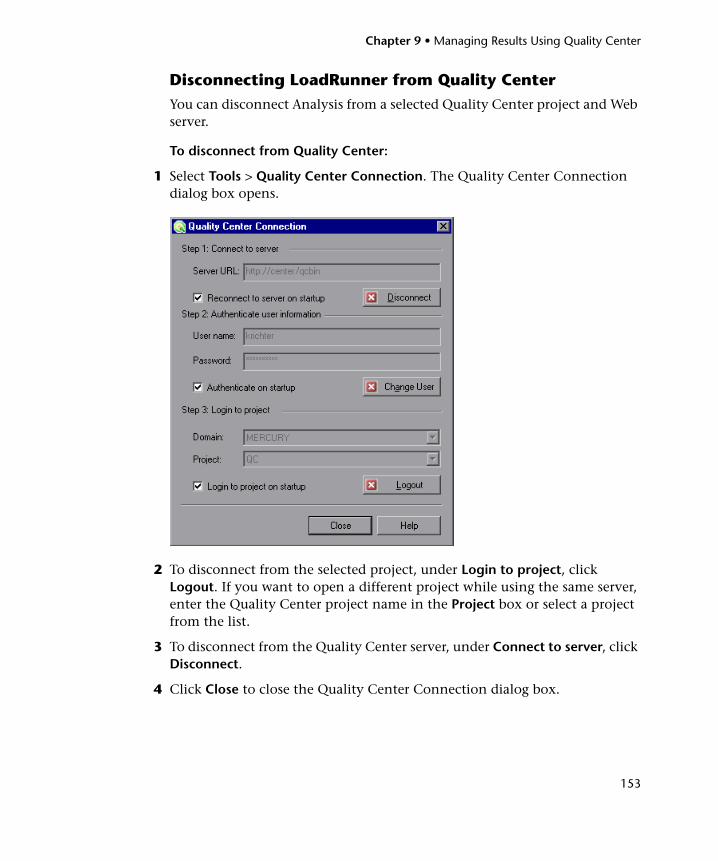
Chapter 9 • Managing Results Using Quality Center
153
Disconnecting LoadRunner from Quality CenterYou can disconnect Analysis from a selected Quality Center project and Web server.
To disconnect from Quality Center:
1 Select Tools > Quality Center Connection. The Quality Center Connection dialog box opens.
2 To disconnect from the selected project, under Login to project, click Logout. If you want to open a different project while using the same server, enter the Quality Center project name in the Project box or select a project from the list.
3 To disconnect from the Quality Center server, under Connect to server, click Disconnect.
4 Click Close to close the Quality Center Connection dialog box.
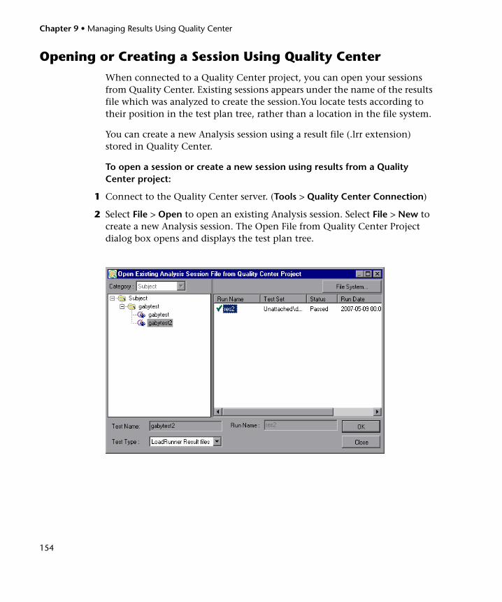
Chapter 9 • Managing Results Using Quality Center
154
Opening or Creating a Session Using Quality Center
When connected to a Quality Center project, you can open your sessions from Quality Center. Existing sessions appears under the name of the results file which was analyzed to create the session.You locate tests according to their position in the test plan tree, rather than a location in the file system.
You can create a new Analysis session using a result file (.lrr extension) stored in Quality Center.
To open a session or create a new session using results from a Quality Center project:
1 Connect to the Quality Center server. (Tools > Quality Center Connection)
2 Select File > Open to open an existing Analysis session. Select File > New to create a new Analysis session. The Open File from Quality Center Project dialog box opens and displays the test plan tree.
Chapter 9 • Managing Results Using Quality Center
155
Note: To open a session/result directly from the file system, click the File System button. (To return to the Open from Quality Center Project dialog box, click the Quality Center button.)
3 Click the relevant subject in the test plan tree. To expand the tree and view sublevels, double-click closed folders. To collapse the tree, double-click open folders.
Note that when you select a subject, the sessions/results that belong to the subject appear in the Run Name list.
4 Select a session/result from the Run Name list. The session appears under the name of the results file which was analyzed to create the session.
5 Click OK. If you are opening an existing session, Analysis loads the session and displays its name in the title bar. If you are creating a new session, Analysis analyzes the results file and creates a new session.
Chapter 9 • Managing Results Using Quality Center
156
Saving Sessions to a Quality Center Project
When Analysis is connected to a Quality Center project, you can create new sessions in Analysis and save them directly to your project.
Important: You can save Analysis sessions to Quality Center only when the session was created from a results file that was stored in Quality Center.
To save a session to a Quality Center project:
1 Connect to the Quality Center server. For more information, see “Connecting to Quality Center” on page 150.
2 Select File > Save and save the session in the Quality Center data directory.
157
10Using Analysis with Performance Center
Note: This chapter is intended specifically for Performance Center users who are using the Analysis Standalone application to analyze load test results.
When a load test is finished, Performance Center automatically organizes the load test data. Using LoadRunner Analysis, the data generated during the load test can be analyzed, and placed into various graphs and reports, or downloaded to a local machine for analysis, and then uploaded back to Performance Center.
This chapter includes:
➤ About Using Analysis with Performance Center on page 158
➤ Connecting Analysis to Performance Center on page 159
➤ Disconnecting Analysis from Performance Center on page 161
➤ Downloading Result and Session Files on page 162
➤ Uploading Session Files and Reports on page 165
Chapter 10 • Using Analysis with Performance Center
158
About Using Analysis with Performance Center
LoadRunner Analysis enables you to analyze load test data off-line, from any computer on which Analysis is installed.
LoadRunner Analysis integrates with Performance Center to let you quickly and easily analyze data collected during a Performance Center run. You download result and session files for analysis on a local Analysis machine. After analyzing the data, you can upload the session files and reports (HTML and Word) to Performance Center to share the results with other users. The files and reports are available from the Load Test Results page.
In order for Analysis to access a Performance Center project, your version of Analysis must be properly configured so that you can connect Analysis to Performance Center.
Note: You must have the latest Standalone Analysis installation of Analysis to use this feature.
To check for proper upload/download configuration in Analysis:
1 Start Analysis.
2 Select Tools.
If the menu item Performance Center Connection is available on the drop-down menu, your version of Analysis is enabled to upload/download Analysis files.
If your version of Analysis is not enabled to do uploads/downloads, or if you do not have Analysis installed on your machine, you need to install the latest version of Analysis.
Note: It is recommended that you first uninstall your older version. To uninstall Analysis, choose the uninstall option under Analysis from the Start menu.
Chapter 10 • Using Analysis with Performance Center
159
To install a newer version of Analysis in Performance Center:
1 From the Miscellaneous menu, select Downloads.
2 Install the Standalone Analysis download.
3 Follow the download instructions.
Once you have a version of Analysis that is enabled, you can connect Analysis to Performance Center and upload/download files.
Connecting Analysis to Performance Center
You can connect or disconnect Analysis from a Performance Center project at any time during an Analysis session.
The connection process has two stages. First, you connect Analysis to a local or remote Performance Center Web server. This server handles the connections between Analysis and the Performance Center project. You connect to Performance Center from the Configure Performance Center Connection dialog box.
Next, you choose the Performance Center project, load test, and run folder from or to which you want Analysis to download or upload files.
Note: Performance Center projects are password protected, so you must provide a user name and a password.
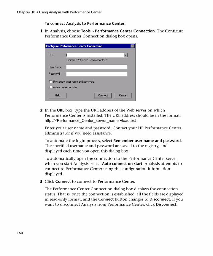
Chapter 10 • Using Analysis with Performance Center
160
To connect Analysis to Performance Center:
1 In Analysis, choose Tools > Performance Center Connection. The Configure Performance Center Connection dialog box opens.
2 In the URL box, type the URL address of the Web server on which Performance Center is installed. The URL address should be in the format: http://<Performance_Center_server_name>/loadtest
Enter your user name and password. Contact your HP Performance Center administrator if you need assistance.
To automate the login process, select Remember user name and password. The specified username and password are saved to the registry, and displayed each time you open this dialog box.
To automatically open the connection to the Performance Center server when you start Analysis, select Auto connect on start. Analysis attempts to connect to Performance Center using the configuration information displayed.
3 Click Connect to connect to Performance Center.
The Performance Center Connection dialog box displays the connection status. That is, once the connection is established, all the fields are displayed in read-only format, and the Connect button changes to Disconnect. If you want to disconnect Analysis from Performance Center, click Disconnect.
Chapter 10 • Using Analysis with Performance Center
161
Note: You cannot be connected to Performance Center and TestDirector at the same time.
Disconnecting Analysis from Performance Center
You disconnect Analysis from the Performance Center Web server using the Configure Performance Center Connection dialog box.
To disconnect Analysis from Performance Center:
1 In Analysis, choose Tools > Performance Center Connection. The Configure Performance Center Connection dialog box opens.
2 Click Disconnect. Analysis disconnects from Performance Center, and the dialog box closes.
Chapter 10 • Using Analysis with Performance Center
162
Downloading Result and Session Files
When Analysis is connected to a Performance Center project, you can download Analysis result and session files stored on the Performance Center server. You locate result and session files according to their position in the projects tree.
When downloading a new session, Analysis prompts you for the load test scenario result file (.lrr extension) to include in the download. To download an existing Analysis session with display information and layout settings for the active graphs, you specify an Analysis Session file (.lra extension).
To download a results file to Analysis:
1 Connect to the Performance Center server. For more information, see “Connecting Analysis to Performance Center” on page 159.
2 In Analysis, choose File > New. The Open Result File for New Analysis Session dialog box opens and displays the load test project tree on the Performance Center server.
Chapter 10 • Using Analysis with Performance Center
163
Note: Performance Center displays only those projects that the user has permission to access.
3 Select the relevant result file by browsing the project, test, and run folders in the projects tree. Result files are identified by a result icon.
To expand the tree and view sublevels, double-click closed folders. To collapse the tree, double-click open folders.
If you want to open a result file from the file system (while connected to Performance Center), click File System. The Open Result File for New Analysis Session dialog box opens displaying the file system. Browse to the directory of the file that you want to open, and click Open.
4 Click OK to download the file and analyze the results. A progress indicator displays the progress of the download.
The downloaded result file is saved to your temp directory. If the download fails, an informative error message is displayed.
Chapter 10 • Using Analysis with Performance Center
164
To download a session file to Analysis:
1 Connect to the Performance Center server. For more information, see “Connecting Analysis to Performance Center” on page 159.
2 In Analysis, choose File > Open. The Open Session dialog box opens and displays the load test project tree on the Performance Center server.
Note: Performance Center displays only those projects that the user has permission to access.
3 Select the relevant session file by browsing the project, test, and run folders in the projects tree. Session files are identified by a session icon.
To expand the tree and view sublevels, double-click closed folders. To collapse the tree, double-click open folders.
If you want to open a session file from the file system (while connected to Performance Center), click File System. The Open Existing Analysis Session File dialog box opens displaying the file system. Browse to the directory of the file that you want to open, and click Open.
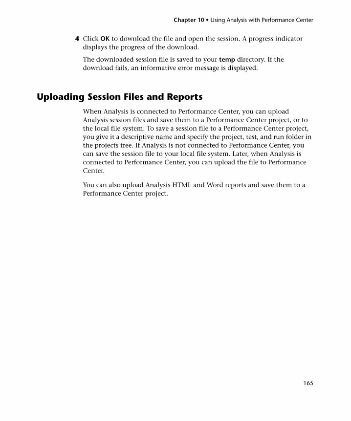
Chapter 10 • Using Analysis with Performance Center
165
4 Click OK to download the file and open the session. A progress indicator displays the progress of the download.
The downloaded session file is saved to your temp directory. If the download fails, an informative error message is displayed.
Uploading Session Files and Reports
When Analysis is connected to Performance Center, you can upload Analysis session files and save them to a Performance Center project, or to the local file system. To save a session file to a Performance Center project, you give it a descriptive name and specify the project, test, and run folder in the projects tree. If Analysis is not connected to Performance Center, you can save the session file to your local file system. Later, when Analysis is connected to Performance Center, you can upload the file to Performance Center.
You can also upload Analysis HTML and Word reports and save them to a Performance Center project.
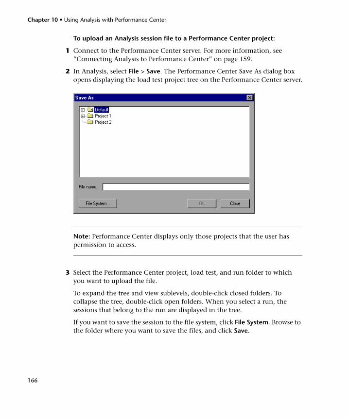
Chapter 10 • Using Analysis with Performance Center
166
To upload an Analysis session file to a Performance Center project:
1 Connect to the Performance Center server. For more information, see “Connecting Analysis to Performance Center” on page 159.
2 In Analysis, select File > Save. The Performance Center Save As dialog box opens displaying the load test project tree on the Performance Center server.
Note: Performance Center displays only those projects that the user has permission to access.
3 Select the Performance Center project, load test, and run folder to which you want to upload the file.
To expand the tree and view sublevels, double-click closed folders. To collapse the tree, double-click open folders. When you select a run, the sessions that belong to the run are displayed in the tree.
If you want to save the session to the file system, click File System. Browse to the folder where you want to save the files, and click Save.
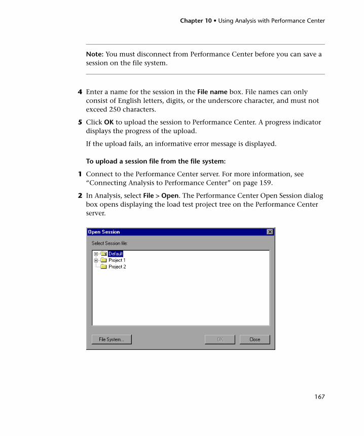
Chapter 10 • Using Analysis with Performance Center
167
Note: You must disconnect from Performance Center before you can save a session on the file system.
4 Enter a name for the session in the File name box. File names can only consist of English letters, digits, or the underscore character, and must not exceed 250 characters.
5 Click OK to upload the session to Performance Center. A progress indicator displays the progress of the upload.
If the upload fails, an informative error message is displayed.
To upload a session file from the file system:
1 Connect to the Performance Center server. For more information, see “Connecting Analysis to Performance Center” on page 159.
2 In Analysis, select File > Open. The Performance Center Open Session dialog box opens displaying the load test project tree on the Performance Center server.
Chapter 10 • Using Analysis with Performance Center
168
3 Click File System. The Open Existing Analysis Session File dialog box opens.
4 Browse to the folder where the session file is saved, and click Open. The session opens in Analysis.
5 Select File > Save As. The Performance Center Save As dialog box opens displaying the load test project tree on the Performance Center server.
6 Continue with the upload procedures from step 3 of “Uploading Session Files and Reports” on page 165.
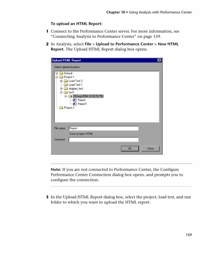
Chapter 10 • Using Analysis with Performance Center
169
To upload an HTML Report:
1 Connect to the Performance Center server. For more information, see “Connecting Analysis to Performance Center” on page 159.
2 In Analysis, select File > Upload to Performance Center > New HTML Report. The Upload HTML Report dialog box opens.
Note: If you are not connected to Performance Center, the Configure Performance Center Connection dialog box opens, and prompts you to configure the connection.
3 In the Upload HTML Report dialog box, select the project, load test, and run folder to which you want to upload the HTML report.
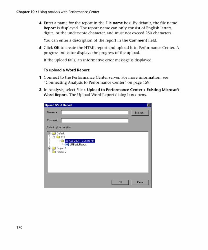
Chapter 10 • Using Analysis with Performance Center
170
4 Enter a name for the report in the File name box. By default, the file name Report is displayed. The report name can only consist of English letters, digits, or the underscore character, and must not exceed 250 characters.
You can enter a description of the report in the Comment field.
5 Click OK to create the HTML report and upload it to Performance Center. A progress indicator displays the progress of the upload.
If the upload fails, an informative error message is displayed.
To upload a Word Report:
1 Connect to the Performance Center server. For more information, see “Connecting Analysis to Performance Center” on page 159.
2 In Analysis, select File > Upload to Performance Center > Existing Microsoft Word Report. The Upload Word Report dialog box opens.
Chapter 10 • Using Analysis with Performance Center
171
Note: If you are not connected to Performance Center, the Configure Performance Center Connection dialog box opens, and prompts you to configure the connection.
3 Click the Browse button, and navigate to the Word report that you want to upload. The path of the selected report is displayed in the File name box.
You can add a description of the report in the Comment box.
4 In the Select upload location section, select the project, load test, and run folder to which you want to upload the report.
5 Click OK. Analysis uploads the Word report to Performance Center. A progress indicator displays the progress of the upload.
If the upload fails, an informative error message is displayed.
Chapter 10 • Using Analysis with Performance Center
172
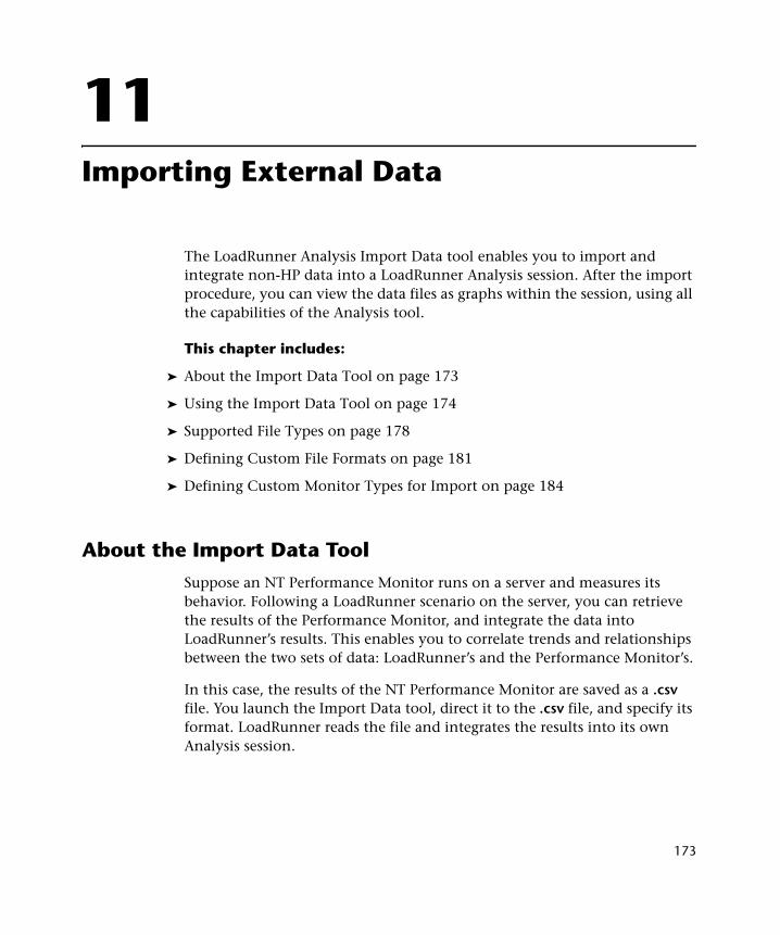
173
11 Importing External Data
The LoadRunner Analysis Import Data tool enables you to import and integrate non-HP data into a LoadRunner Analysis session. After the import procedure, you can view the data files as graphs within the session, using all the capabilities of the Analysis tool.
This chapter includes:
➤ About the Import Data Tool on page 173
➤ Using the Import Data Tool on page 174
➤ Supported File Types on page 178
➤ Defining Custom File Formats on page 181
➤ Defining Custom Monitor Types for Import on page 184
About the Import Data Tool
Suppose an NT Performance Monitor runs on a server and measures its behavior. Following a LoadRunner scenario on the server, you can retrieve the results of the Performance Monitor, and integrate the data into LoadRunner’s results. This enables you to correlate trends and relationships between the two sets of data: LoadRunner’s and the Performance Monitor’s.
In this case, the results of the NT Performance Monitor are saved as a .csv file. You launch the Import Data tool, direct it to the .csv file, and specify its format. LoadRunner reads the file and integrates the results into its own Analysis session.
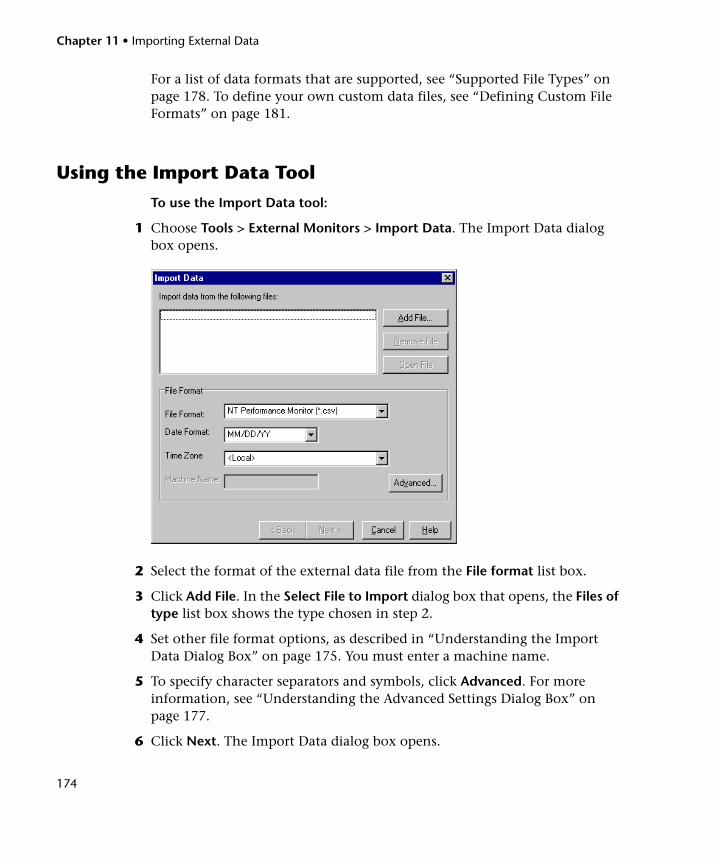
Chapter 11 • Importing External Data
174
For a list of data formats that are supported, see “Supported File Types” on page 178. To define your own custom data files, see “Defining Custom File Formats” on page 181.
Using the Import Data Tool
To use the Import Data tool:
1 Choose Tools > External Monitors > Import Data. The Import Data dialog box opens.
2 Select the format of the external data file from the File format list box.
3 Click Add File. In the Select File to Import dialog box that opens, the Files of type list box shows the type chosen in step 2.
4 Set other file format options, as described in “Understanding the Import Data Dialog Box” on page 175. You must enter a machine name.
5 To specify character separators and symbols, click Advanced. For more information, see “Understanding the Advanced Settings Dialog Box” on page 177.
6 Click Next. The Import Data dialog box opens.
Chapter 11 • Importing External Data
175
7 Select the type of monitor that generated the external data file. If your monitor type does not exist, you can add it, as described in “Defining Custom Monitor Types for Import” on page 184.
When opening a new graph, you will see your monitor added to the list of available graphs under this particular category. (See “Accessing and Opening Graphs and Reports” on page 30.)
8 Click Finish. LoadRunner Analysis imports the data file or files, and refreshes all graphs currently displayed in the session.
Note: When importing data into a scenario with two or more cross results, the imported data will be integrated into the last set of results listed in the File > Cross with Result dialog box. For more information, see “Generating Cross Result Graphs” on page 130.
Understanding the Import Data Dialog BoxYou use the Import Data dialog box to import and integrate non-HP data files into a Analysis session.
➤ Import data from the following files. Displays the files that you selected for import.
➤ Add File. Select an external data file to import. A dialog box opens to enable you to select files.
➤ Remove File. Delete an external data file from the list.
➤ Open File. Open an external data file using the associated application.
➤ File Format. Set the file format options.
➤ File Format. Choose the format of the external data file. For an explanation of available formats, see “Supported File Types” on page 178.
➤ Date Format. Specify the format of the date in the imported data file. For example, for European dates with a 4 digit year, choose DD/MM/YYYY.
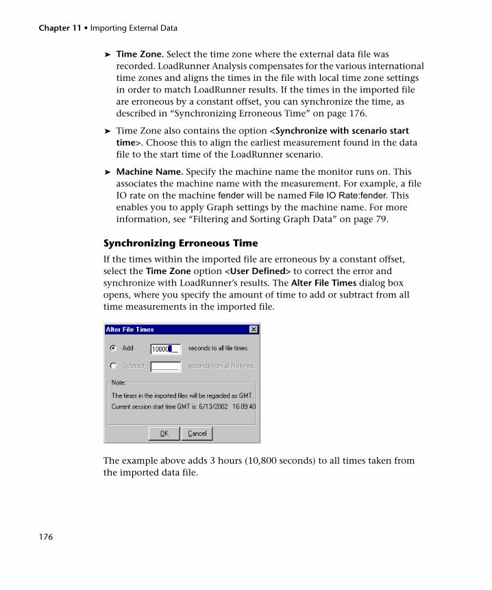
Chapter 11 • Importing External Data
176
➤ Time Zone. Select the time zone where the external data file was recorded. LoadRunner Analysis compensates for the various international time zones and aligns the times in the file with local time zone settings in order to match LoadRunner results. If the times in the imported file are erroneous by a constant offset, you can synchronize the time, as described in “Synchronizing Erroneous Time” on page 176.
➤ Time Zone also contains the option <Synchronize with scenario start time>. Choose this to align the earliest measurement found in the data file to the start time of the LoadRunner scenario.
➤ Machine Name. Specify the machine name the monitor runs on. This associates the machine name with the measurement. For example, a file IO rate on the machine fender will be named File IO Rate:fender. This enables you to apply Graph settings by the machine name. For more information, see “Filtering and Sorting Graph Data” on page 79.
Synchronizing Erroneous Time
If the times within the imported file are erroneous by a constant offset, select the Time Zone option <User Defined> to correct the error and synchronize with LoadRunner’s results. The Alter File Times dialog box opens, where you specify the amount of time to add or subtract from all time measurements in the imported file.
The example above adds 3 hours (10,800 seconds) to all times taken from the imported data file.
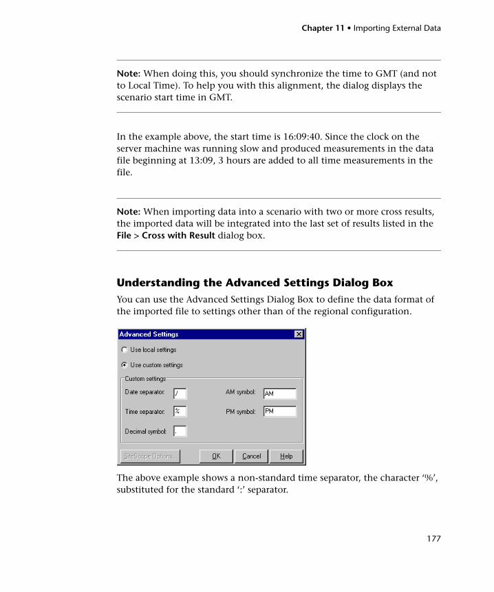
Chapter 11 • Importing External Data
177
Note: When doing this, you should synchronize the time to GMT (and not to Local Time). To help you with this alignment, the dialog displays the scenario start time in GMT.
In the example above, the start time is 16:09:40. Since the clock on the server machine was running slow and produced measurements in the data file beginning at 13:09, 3 hours are added to all time measurements in the file.
Note: When importing data into a scenario with two or more cross results, the imported data will be integrated into the last set of results listed in the File > Cross with Result dialog box.
Understanding the Advanced Settings Dialog BoxYou can use the Advanced Settings Dialog Box to define the data format of the imported file to settings other than of the regional configuration.
The above example shows a non-standard time separator, the character ‘%’, substituted for the standard ‘:’ separator.
Chapter 11 • Importing External Data
178
Use local settings. Keep default settings of the regional configuration. Disables the Custom Settings area of the dialog box.
Use custom settings. Define your own settings. Enables the Custom Settings area of the dialog box.
➤ Date Separator. Enter a custom symbol, for example, the slash (‘/’) character in 11/10/02
➤ Time Separator. Enter a custom symbol, for example, the colon ‘:’ character in 9:54:19
➤ Decimal symbol. Enter a custom symbol, for example, the ‘.’ character in the number 2.5
➤ AM symbol. Enter a custom symbol for the hours between midnight and noon.
➤ PM symbol. Enter a custom symbol for the hours between noon and midnight.
Supported File Types
The following file types are supported:
➤ NT Performance Monitor (.csv)
➤ Windows 2000 Performance Monitor (.csv)
➤ Standard Comma Separated File (.csv)
➤ Master-Detail Comma Separated File (.csv)
➤ Microsoft Excel File (.xls)
➤ Master-Detail Microsoft Excel file (.xls)
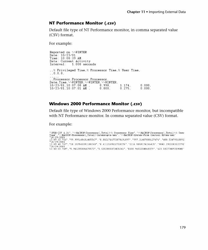
Chapter 11 • Importing External Data
179
NT Performance Monitor (.csv)
Default file type of NT Performance monitor, in comma separated value (CSV) format.
For example:
Windows 2000 Performance Monitor (.csv)
Default file type of Windows 2000 Performance monitor, but incompatible with NT Performance monitor. In comma separated value (CSV) format.
For example:
Chapter 11 • Importing External Data
180
Standard Comma Separated File (.csv)
This file type has the following format:
Date,Time,Measurement_1,Measurement_2, ...
where fields are comma separated and first row contains column titles.
The following example from a standard CSV file shows 3 measurements: an interrupt rate, a file IO rate and a CPU usage. The first row shows an interrupt rate of 1122.19 and an IO rate of 4.18:
Master-Detail Comma Separated File (.csv)
This file type is identical to Standard Comma Separated Files except for an additional Master column which specifies that row’s particular breakdown of a more general measurement. For example, a Standard CSV file may contain data points of a machine’s total CPU usage at a given moment:
Date,Time,CPU_Usage
However, if the total CPU usage can be further broken up into CPU time per-process, then a Master-Detail CSV file can be created with an extra column ProcessName, containing the name of a process.
Each row contains the measurement of a specific process’s CPU usage only. The format will be the following:
Date,Time,ProcessName,CPU_Usage
as in the following example:
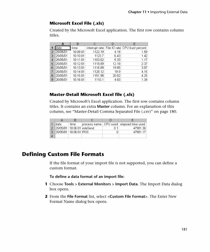
Chapter 11 • Importing External Data
181
Microsoft Excel File (.xls)
Created by the Microsoft Excel application. The first row contains column titles.
Master-Detail Microsoft Excel file (.xls)
Created by Microsoft’s Excel application. The first row contains column titles. It contains an extra Master column. For an explanation of this column, see “Master-Detail Comma Separated File (.csv)” on page 180.
Defining Custom File Formats
If the file format of your import file is not supported, you can define a custom format.
To define a data format of an import file:
1 Choose Tools > External Monitors > Import Data. The Import Data dialog box opens.
2 From the File Format list, select <Custom File Format>. The Enter New Format Name dialog box opens.
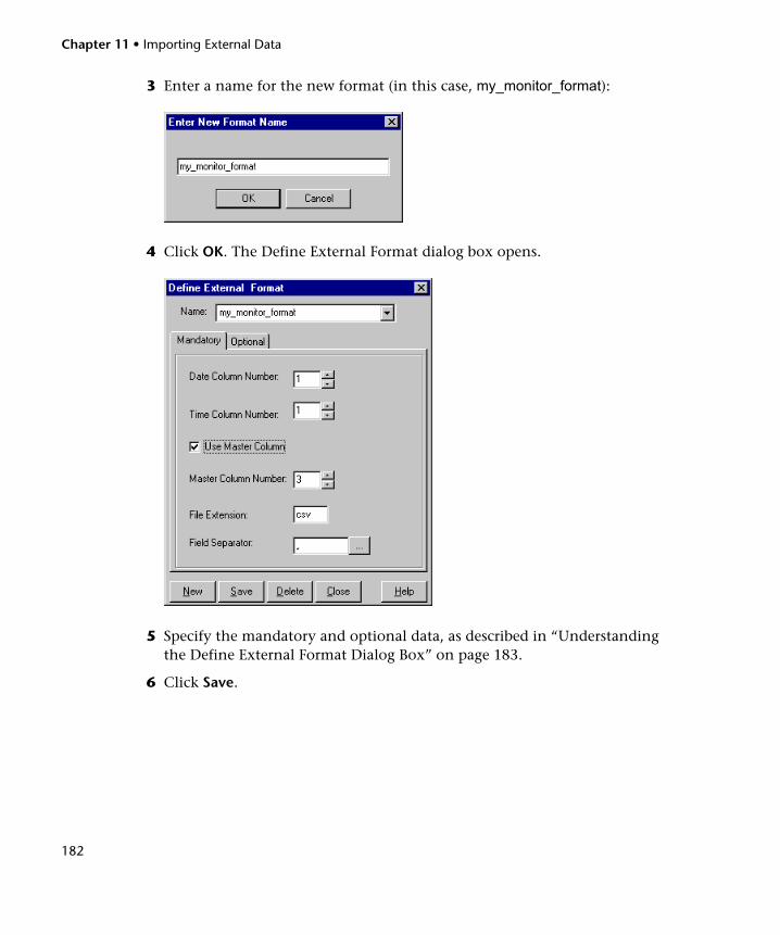
Chapter 11 • Importing External Data
182
3 Enter a name for the new format (in this case, my_monitor_format):
4 Click OK. The Define External Format dialog box opens.
5 Specify the mandatory and optional data, as described in “Understanding the Define External Format Dialog Box” on page 183.
6 Click Save.
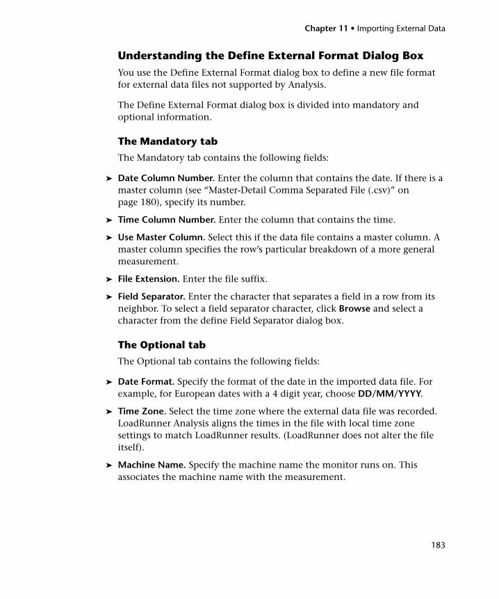
Chapter 11 • Importing External Data
183
Understanding the Define External Format Dialog BoxYou use the Define External Format dialog box to define a new file format for external data files not supported by Analysis.
The Define External Format dialog box is divided into mandatory and optional information.
The Mandatory tab
The Mandatory tab contains the following fields:
➤ Date Column Number. Enter the column that contains the date. If there is a master column (see “Master-Detail Comma Separated File (.csv)” on page 180), specify its number.
➤ Time Column Number. Enter the column that contains the time.
➤ Use Master Column. Select this if the data file contains a master column. A master column specifies the row’s particular breakdown of a more general measurement.
➤ File Extension. Enter the file suffix.
➤ Field Separator. Enter the character that separates a field in a row from its neighbor. To select a field separator character, click Browse and select a character from the define Field Separator dialog box.
The Optional tab
The Optional tab contains the following fields:
➤ Date Format. Specify the format of the date in the imported data file. For example, for European dates with a 4 digit year, choose DD/MM/YYYY.
➤ Time Zone. Select the time zone where the external data file was recorded. LoadRunner Analysis aligns the times in the file with local time zone settings to match LoadRunner results. (LoadRunner does not alter the file itself).
➤ Machine Name. Specify the machine name the monitor runs on. This associates the machine name with the measurement.
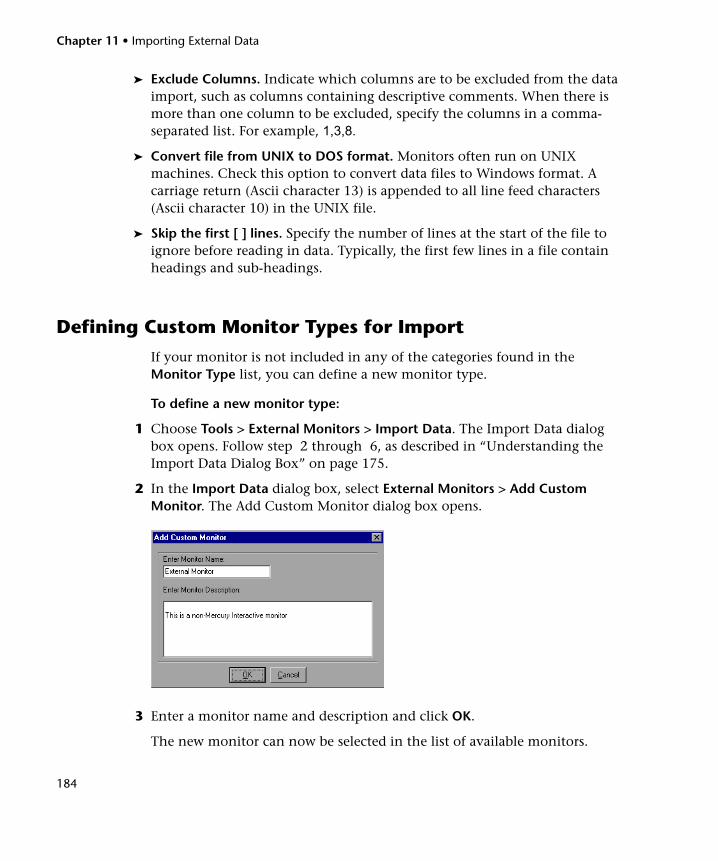
Chapter 11 • Importing External Data
184
➤ Exclude Columns. Indicate which columns are to be excluded from the data import, such as columns containing descriptive comments. When there is more than one column to be excluded, specify the columns in a comma-separated list. For example, 1,3,8.
➤ Convert file from UNIX to DOS format. Monitors often run on UNIX machines. Check this option to convert data files to Windows format. A carriage return (Ascii character 13) is appended to all line feed characters (Ascii character 10) in the UNIX file.
➤ Skip the first [ ] lines. Specify the number of lines at the start of the file to ignore before reading in data. Typically, the first few lines in a file contain headings and sub-headings.
Defining Custom Monitor Types for Import
If your monitor is not included in any of the categories found in the Monitor Type list, you can define a new monitor type.
To define a new monitor type:
1 Choose Tools > External Monitors > Import Data. The Import Data dialog box opens. Follow step 2 through 6, as described in “Understanding the Import Data Dialog Box” on page 175.
2 In the Import Data dialog box, select External Monitors > Add Custom Monitor. The Add Custom Monitor dialog box opens.
3 Enter a monitor name and description and click OK.
The new monitor can now be selected in the list of available monitors.
Part II
Analysis Graphs

186
187
12 Vuser Graphs
After running a load test scenario, you can check the behavior of the Vusers that participated in the scenario using the Vuser graphs.
This chapter includes:
➤ About Vuser Graphs on page 187
➤ Running Vusers Graph on page 188
➤ Vuser Summary Graph on page 189
➤ Rendezvous Graph on page 190
About Vuser Graphs
During load test scenario execution, Vusers generate data as they perform transactions. The Vuser graphs let you determine the overall behavior of Vusers during the scenario. They display the Vuser states, the number of Vusers that completed the script, and rendezvous statistics. Use these graphs in conjunction with Transaction graphs to determine the effect of the number of Vusers on transaction response time.
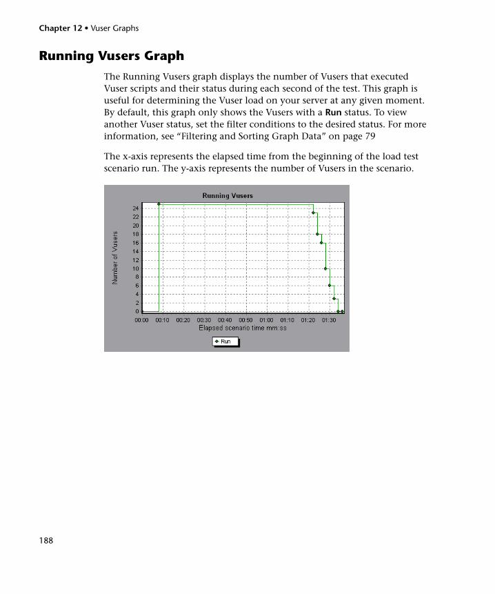
Chapter 12 • Vuser Graphs
188
Running Vusers Graph
The Running Vusers graph displays the number of Vusers that executed Vuser scripts and their status during each second of the test. This graph is useful for determining the Vuser load on your server at any given moment. By default, this graph only shows the Vusers with a Run status. To view another Vuser status, set the filter conditions to the desired status. For more information, see “Filtering and Sorting Graph Data” on page 79
The x-axis represents the elapsed time from the beginning of the load test scenario run. The y-axis represents the number of Vusers in the scenario.
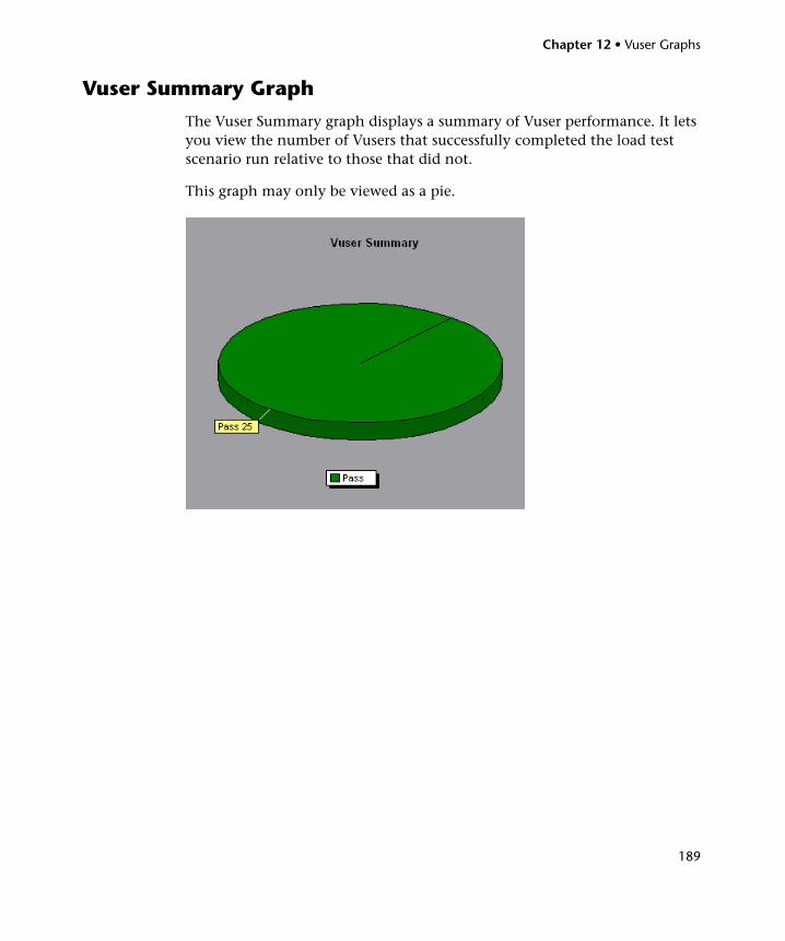
Chapter 12 • Vuser Graphs
189
Vuser Summary Graph
The Vuser Summary graph displays a summary of Vuser performance. It lets you view the number of Vusers that successfully completed the load test scenario run relative to those that did not.
This graph may only be viewed as a pie.
Chapter 12 • Vuser Graphs
190
Rendezvous Graph
The Rendezvous graph indicates when Vusers were released from rendezvous points, and how many Vusers were released at each point.
This graph helps you understand transaction performance times. If you compare the Rendezvous graph to the Average Transaction Response Time graph, you can see how the load peak created by a rendezvous influences transaction times.
On the Rendezvous graph, the x-axis indicates the time that elapsed since the beginning of the load test scenario. The y-axis indicates the number of Vusers that were released from the rendezvous. If you set a rendezvous for 60 Vusers, and the graph indicates that only 25 were released, you can see that the rendezvous ended when the timeout expired because all of the Vusers did not arrive.
191
13 Error Graphs
After a load test scenario run, you can use the Error graphs to analyze the errors that occurred during the load test.
This chapter includes:
➤ About Error Graphs on page 191
➤ Error Statistics Graph on page 192
➤ Error Statistics (by Description) Graph on page 193
➤ Total Errors per Second Graph on page 194
➤ Errors per Second Graph on page 195
➤ Errors per Second (by Description) Graph on page 196
About Error Graphs
During load test scenario execution, Vusers may not complete all transactions successfully. The Error graphs let you view information about the transactions that failed, stopped, or ended in errors. Using the Error graphs, you can view a summary of errors that occurred during the scenario and the average number of errors that occurred per second.
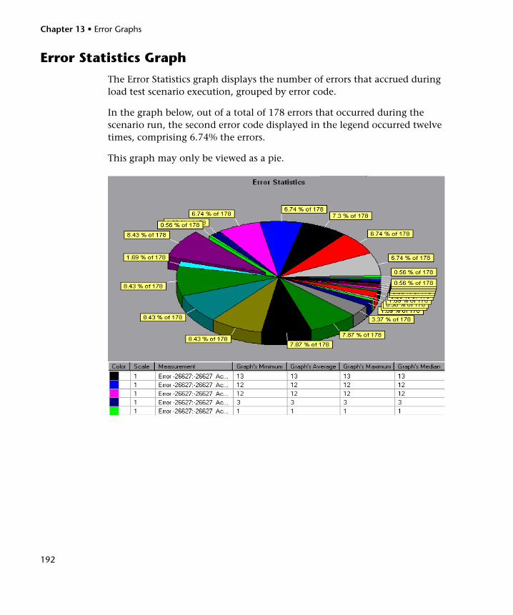
Chapter 13 • Error Graphs
192
Error Statistics Graph
The Error Statistics graph displays the number of errors that accrued during load test scenario execution, grouped by error code.
In the graph below, out of a total of 178 errors that occurred during the scenario run, the second error code displayed in the legend occurred twelve times, comprising 6.74% the errors.
This graph may only be viewed as a pie.
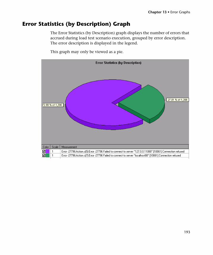
Chapter 13 • Error Graphs
193
Error Statistics (by Description) Graph
The Error Statistics (by Description) graph displays the number of errors that accrued during load test scenario execution, grouped by error description. The error description is displayed in the legend.
This graph may only be viewed as a pie.
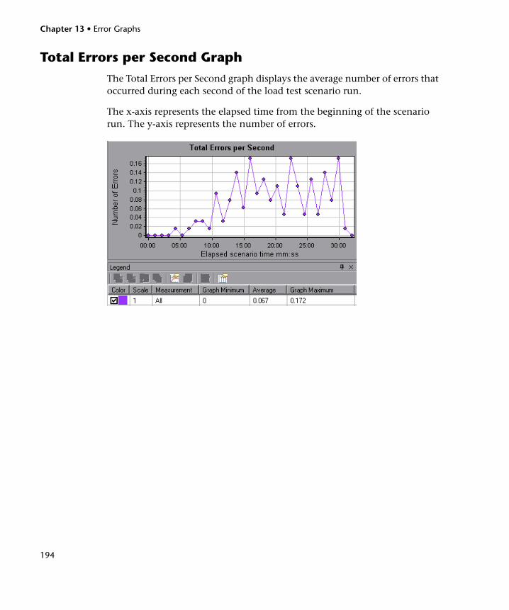
Chapter 13 • Error Graphs
194
Total Errors per Second Graph
The Total Errors per Second graph displays the average number of errors that occurred during each second of the load test scenario run.
The x-axis represents the elapsed time from the beginning of the scenario run. The y-axis represents the number of errors.

Chapter 13 • Error Graphs
195
Errors per Second Graph
The Errors per Second graph displays the average number of errors that occurred during each second of the load test scenario run, grouped by error code.
The x-axis represents the elapsed time from the beginning of the scenario run. The y-axis represents the number of errors.
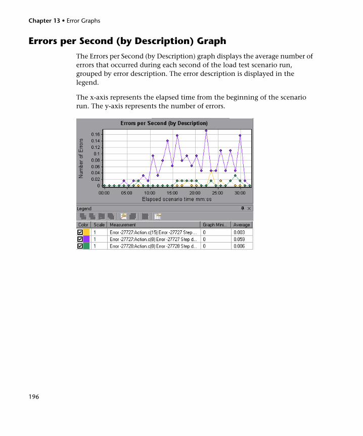
Chapter 13 • Error Graphs
196
Errors per Second (by Description) Graph
The Errors per Second (by Description) graph displays the average number of errors that occurred during each second of the load test scenario run, grouped by error description. The error description is displayed in the legend.
The x-axis represents the elapsed time from the beginning of the scenario run. The y-axis represents the number of errors.
197
14Transaction Graphs
After running a load test scenario, you can analyze the transactions that were executed during the test using the Transaction graphs.
This chapter includes:
➤ About Transaction Graphs on page 197
➤ Average Transaction Response Time Graph on page 198
➤ Transactions per Second Graph on page 201
➤ Total Transactions per Second Graph on page 202
➤ Transaction Summary Graph on page 203
➤ Transaction Performance Summary Graph on page 204
➤ Transaction Response Time (Under Load) Graph on page 205
➤ Transaction Response Time (Percentile) Graph on page 206
➤ Transaction Response Time (Distribution) Graph on page 208
About Transaction Graphs
During load test scenario execution, Vusers generate data as they perform transactions. Analysis enables you to generate graphs that show the transaction performance and status throughout script execution.
You can use additional Analysis tools such as merging and crossing results to understand your transaction performance graphs. You can also sort the graph information by transactions. For more information about working with Analysis, see Part I, “Working with Analysis”
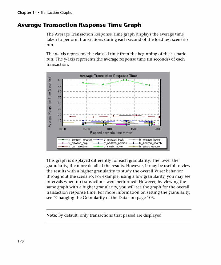
Chapter 14 • Transaction Graphs
198
Average Transaction Response Time Graph
The Average Transaction Response Time graph displays the average time taken to perform transactions during each second of the load test scenario run.
The x-axis represents the elapsed time from the beginning of the scenario run. The y-axis represents the average response time (in seconds) of each transaction.
This graph is displayed differently for each granularity. The lower the granularity, the more detailed the results. However, it may be useful to view the results with a higher granularity to study the overall Vuser behavior throughout the scenario. For example, using a low granularity, you may see intervals when no transactions were performed. However, by viewing the same graph with a higher granularity, you will see the graph for the overall transaction response time. For more information on setting the granularity, see “Changing the Granularity of the Data” on page 105.
Note: By default, only transactions that passed are displayed.
Chapter 14 • Transaction Graphs
199
You can view a breakdown of a transaction in the Average Transaction Response Time graph by selecting View > Show Transaction Breakdown Tree, or right-clicking the transaction in the graph and selecting Show Transaction Breakdown Tree. In the Transaction Breakdown Tree, right-click the transaction you want to break down, and select Break Down <transaction name>. The Average Transaction Response Time graph displays data for the sub-transactions.
To view a breakdown of the Web page(s) included in a transaction or sub-transaction, right-click it and select Web Page Diagnostics for <transaction name>.
For more information on the Web Page Diagnostics graphs, see Chapter 16, “Web Page Diagnostics Graphs.”
You can compare the Average Transaction Response Time graph to the Running Vusers graph to see how the number of running Vusers affects the transaction performance time.
For example, if the Average Transaction Response Time graph shows that performance time gradually improved, you can compare it to the Running Vusers graph to see whether the performance time improved due to a decrease in the Vuser load.
If you have defined acceptable minimum and maximum transaction performance times, you can use this graph to determine whether the performance of the server is within the acceptable range.
Understanding the Transaction Breakdown Tree The Transaction Breakdown Tree displays a tree view of the transactions and sub-transactions in the current session.
To expand the view and drill down to the transactions and sub-transactions, click the "+" sign.
To collapse the view, click the "-" sign.
Chapter 14 • Transaction Graphs
200
To view breakdown of a transaction, right-click it and select Break Down <transaction name>. The Average Transaction Response Time or Transaction Performance Summary graph displays data for the sub-transactions. To view data only for the selected transaction/sub-transaction, right-click it and choose Show Only <transaction name>.
To view breakdown of the Web page(s) included in a transaction or sub-transaction, right-click the transaction/sub-transaction, and select Web Page Diagnostics for <page name>.
Understanding the Web Page Diagnostics Tree ViewThe Web Page Diagnostics tree view displays a tree view of the transactions, sub-transactions, and Web pages for which you can view Web Page Diagnostics graphs. For more information about Web Page Diagnostics graphs, see Chapter 16, “Web Page Diagnostics Graphs.”
To expand the view and drill down to the transactions, sub-transactions, Web pages, and page components, click the "+" sign.
To collapse the view, click the "-" sign.
To view breakdown of a transaction or sub-transaction, right-click it and select Web Page Diagnostics for <transaction name>. The Web Page Diagnostics graph opens in the right pane. To view breakdown of a specific Web page, right-click the page and select Break Down <page name>.
Note: You can open a browser displaying the problematic page by right-clicking the page in the Web Page Diagnostics tree and selecting View page in browser.
You can also open a Web Page Diagnostics graph by choosing Graph > Add New Graph > Web Page Diagnostics, and selecting one of the Web Page Diagnostics graphs.
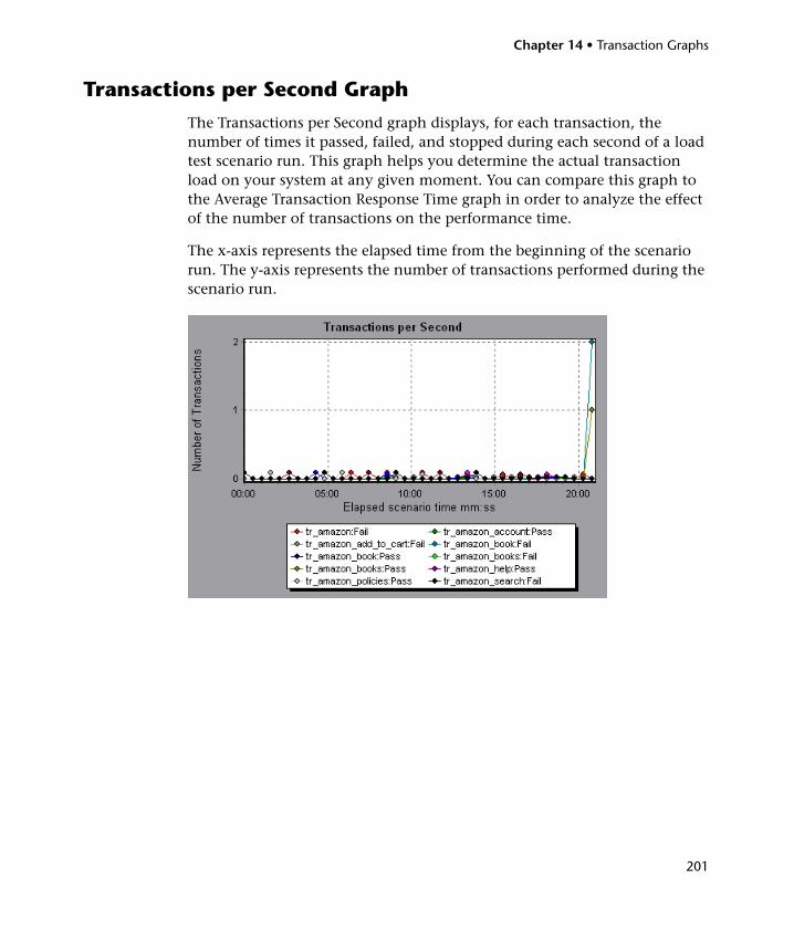
Chapter 14 • Transaction Graphs
201
Transactions per Second Graph
The Transactions per Second graph displays, for each transaction, the number of times it passed, failed, and stopped during each second of a load test scenario run. This graph helps you determine the actual transaction load on your system at any given moment. You can compare this graph to the Average Transaction Response Time graph in order to analyze the effect of the number of transactions on the performance time.
The x-axis represents the elapsed time from the beginning of the scenario run. The y-axis represents the number of transactions performed during the scenario run.
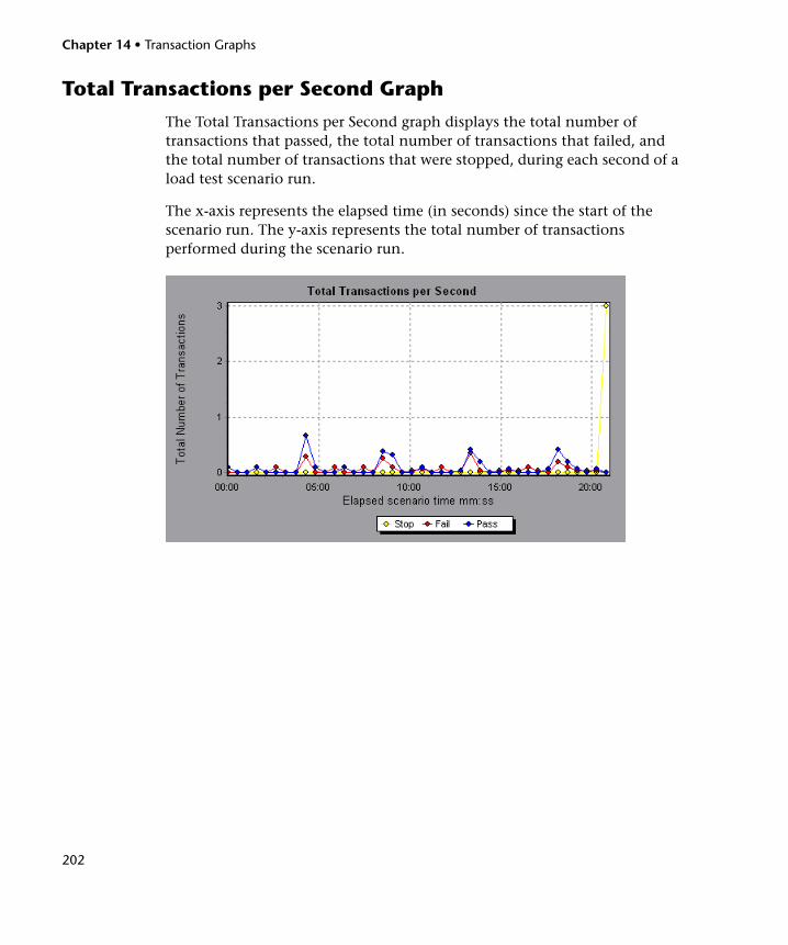
Chapter 14 • Transaction Graphs
202
Total Transactions per Second Graph
The Total Transactions per Second graph displays the total number of transactions that passed, the total number of transactions that failed, and the total number of transactions that were stopped, during each second of a load test scenario run.
The x-axis represents the elapsed time (in seconds) since the start of the scenario run. The y-axis represents the total number of transactions performed during the scenario run.
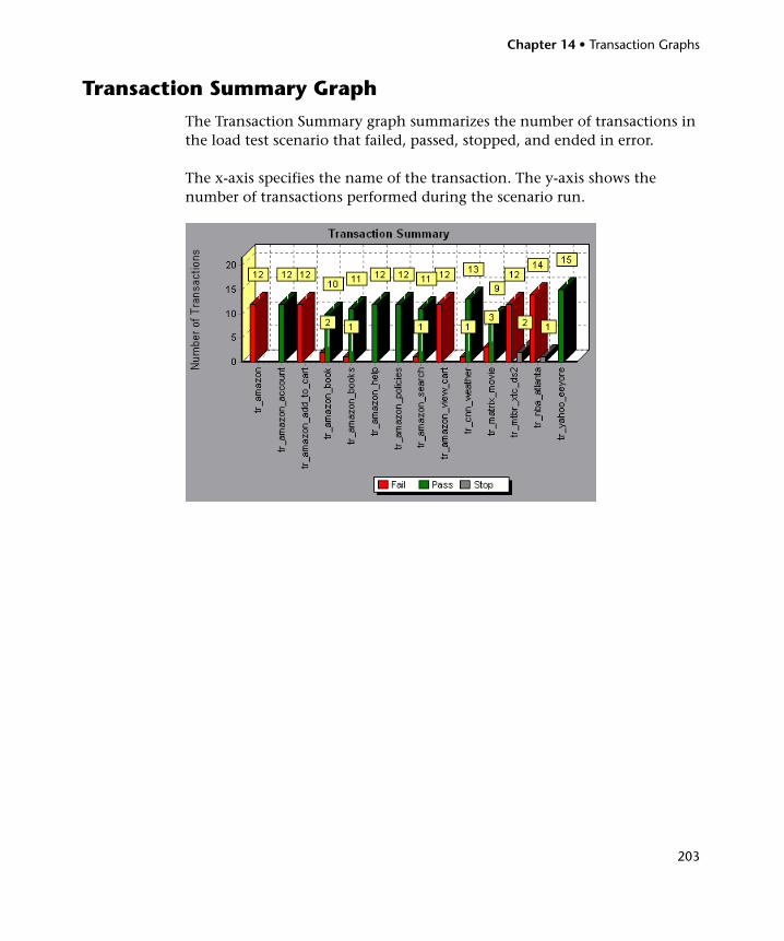
Chapter 14 • Transaction Graphs
203
Transaction Summary Graph
The Transaction Summary graph summarizes the number of transactions in the load test scenario that failed, passed, stopped, and ended in error.
The x-axis specifies the name of the transaction. The y-axis shows the number of transactions performed during the scenario run.
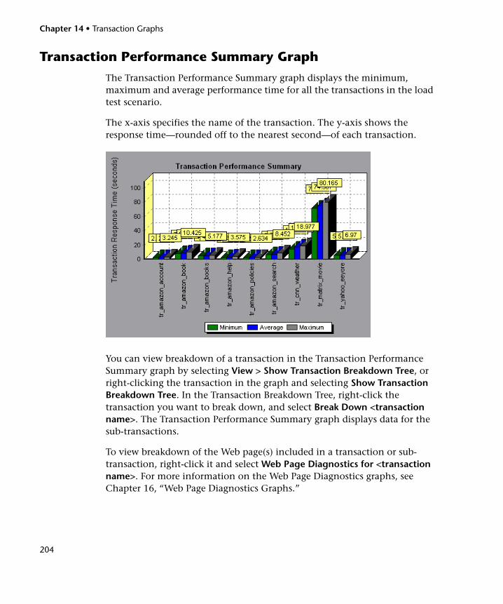
Chapter 14 • Transaction Graphs
204
Transaction Performance Summary Graph
The Transaction Performance Summary graph displays the minimum, maximum and average performance time for all the transactions in the load test scenario.
The x-axis specifies the name of the transaction. The y-axis shows the response time—rounded off to the nearest second—of each transaction.
You can view breakdown of a transaction in the Transaction Performance Summary graph by selecting View > Show Transaction Breakdown Tree, or right-clicking the transaction in the graph and selecting Show Transaction Breakdown Tree. In the Transaction Breakdown Tree, right-click the transaction you want to break down, and select Break Down <transaction name>. The Transaction Performance Summary graph displays data for the sub-transactions.
To view breakdown of the Web page(s) included in a transaction or sub-transaction, right-click it and select Web Page Diagnostics for <transaction name>. For more information on the Web Page Diagnostics graphs, see Chapter 16, “Web Page Diagnostics Graphs.”
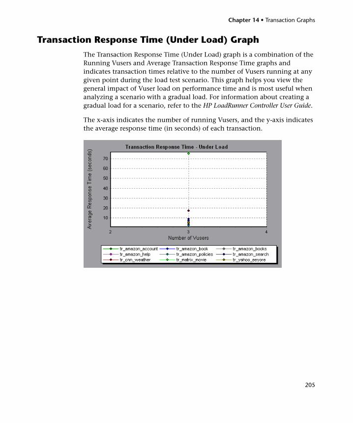
Chapter 14 • Transaction Graphs
205
Transaction Response Time (Under Load) Graph
The Transaction Response Time (Under Load) graph is a combination of the Running Vusers and Average Transaction Response Time graphs and indicates transaction times relative to the number of Vusers running at any given point during the load test scenario. This graph helps you view the general impact of Vuser load on performance time and is most useful when analyzing a scenario with a gradual load. For information about creating a gradual load for a scenario, refer to the HP LoadRunner Controller User Guide.
The x-axis indicates the number of running Vusers, and the y-axis indicates the average response time (in seconds) of each transaction.
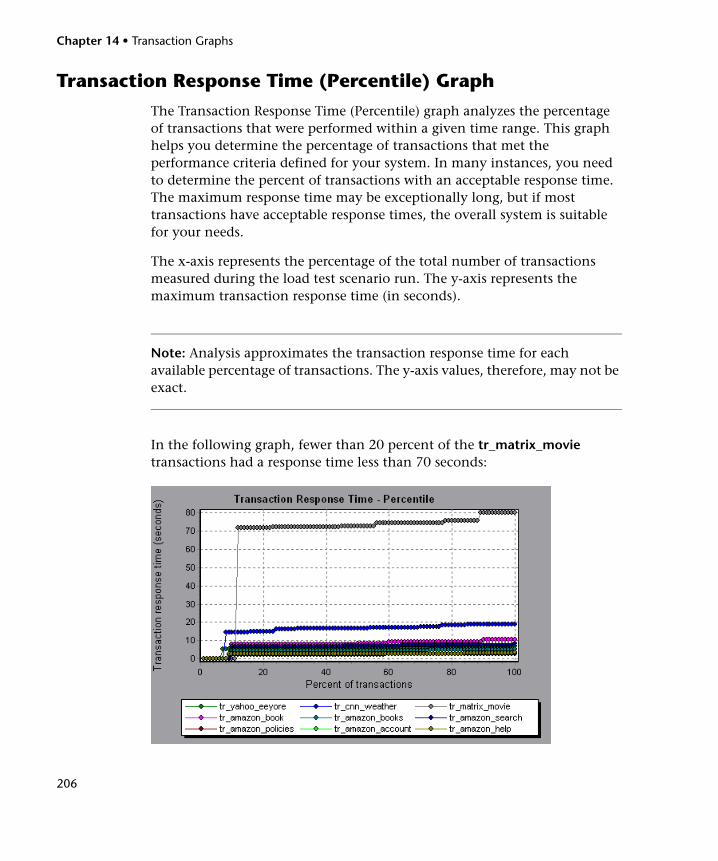
Chapter 14 • Transaction Graphs
206
Transaction Response Time (Percentile) Graph
The Transaction Response Time (Percentile) graph analyzes the percentage of transactions that were performed within a given time range. This graph helps you determine the percentage of transactions that met the performance criteria defined for your system. In many instances, you need to determine the percent of transactions with an acceptable response time. The maximum response time may be exceptionally long, but if most transactions have acceptable response times, the overall system is suitable for your needs.
The x-axis represents the percentage of the total number of transactions measured during the load test scenario run. The y-axis represents the maximum transaction response time (in seconds).
Note: Analysis approximates the transaction response time for each available percentage of transactions. The y-axis values, therefore, may not be exact.
In the following graph, fewer than 20 percent of the tr_matrix_movie transactions had a response time less than 70 seconds:
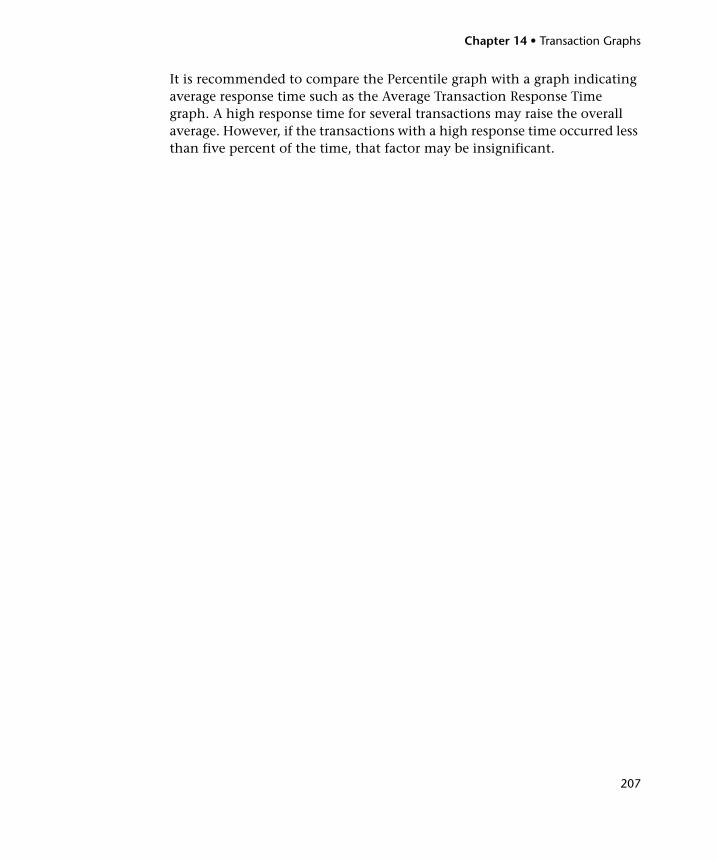
Chapter 14 • Transaction Graphs
207
It is recommended to compare the Percentile graph with a graph indicating average response time such as the Average Transaction Response Time graph. A high response time for several transactions may raise the overall average. However, if the transactions with a high response time occurred less than five percent of the time, that factor may be insignificant.
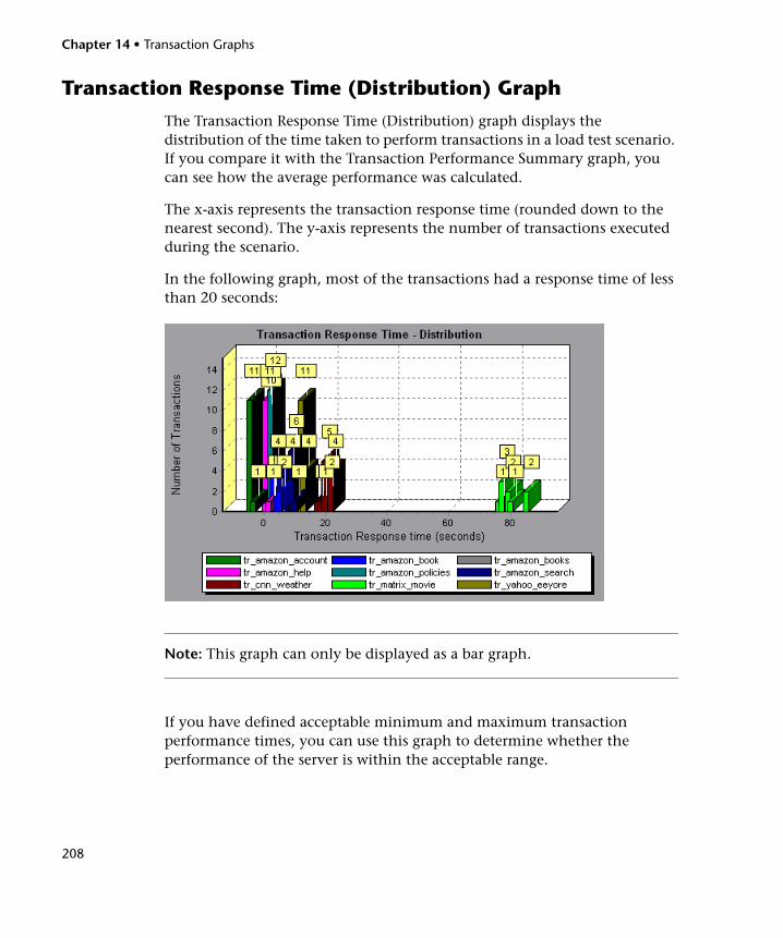
Chapter 14 • Transaction Graphs
208
Transaction Response Time (Distribution) Graph
The Transaction Response Time (Distribution) graph displays the distribution of the time taken to perform transactions in a load test scenario. If you compare it with the Transaction Performance Summary graph, you can see how the average performance was calculated.
The x-axis represents the transaction response time (rounded down to the nearest second). The y-axis represents the number of transactions executed during the scenario.
In the following graph, most of the transactions had a response time of less than 20 seconds:
Note: This graph can only be displayed as a bar graph.
If you have defined acceptable minimum and maximum transaction performance times, you can use this graph to determine whether the performance of the server is within the acceptable range.
209
15 Web Resource Graphs
After a load test scenario run, you can use the Web Resource graphs to analyze Web server performance.
This chapter includes:
➤ About Web Resource Graphs on page 210
➤ Hits per Second Graph on page 211
➤ Throughput Graph on page 212
➤ HTTP Status Code Summary Graph on page 213
➤ HTTP Responses per Second Graph on page 214
➤ Pages Downloaded per Second Graph on page 217
➤ Retries per Second Graph on page 219
➤ Retries Summary Graph on page 220
➤ Connections Graph on page 221
➤ Connections per Second Graph on page 222
➤ SSLs per Second Graph on page 223
Chapter 15 • Web Resource Graphs
210
About Web Resource Graphs
Web Resource graphs provide you with information about the performance of your Web server. You use the Web Resource graphs to analyze the following data:
➤ Throughput on the Web server
➤ The number of hits per second
➤ The number of HTTP responses per second
➤ The HTTP status codes returned from the Web server
➤ The number of downloaded pages per second
➤ The number of server retries per second
➤ A summary of the server retries during the load test scenario
➤ The number of open TCP/IP connections
➤ The number of new TCP/IP connections opened
➤ The number of connections that are shut down
➤ The number of new and reused SSL connections opened
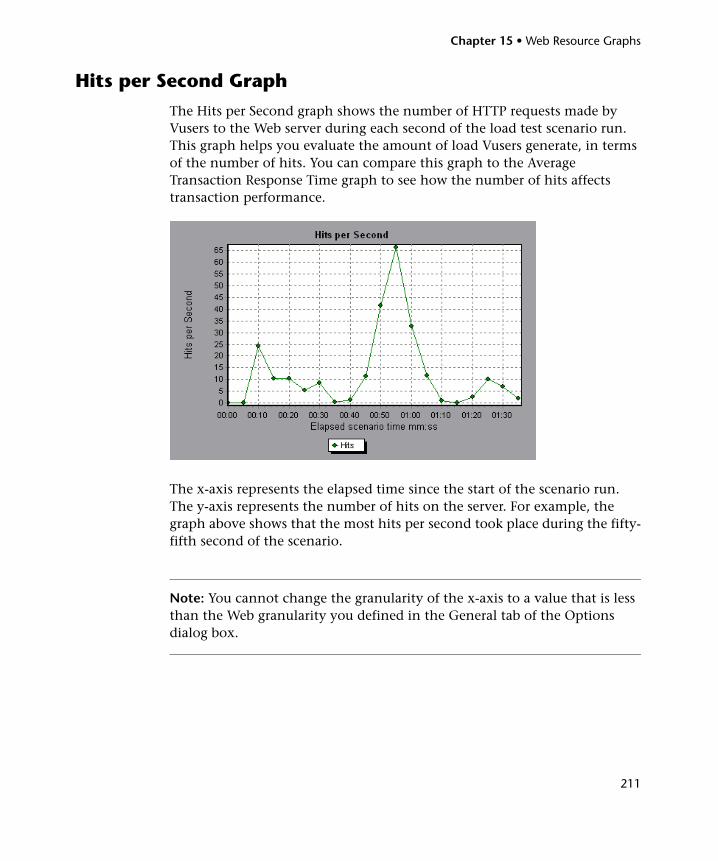
Chapter 15 • Web Resource Graphs
211
Hits per Second Graph
The Hits per Second graph shows the number of HTTP requests made by Vusers to the Web server during each second of the load test scenario run. This graph helps you evaluate the amount of load Vusers generate, in terms of the number of hits. You can compare this graph to the Average Transaction Response Time graph to see how the number of hits affects transaction performance.
The x-axis represents the elapsed time since the start of the scenario run. The y-axis represents the number of hits on the server. For example, the graph above shows that the most hits per second took place during the fifty-fifth second of the scenario.
Note: You cannot change the granularity of the x-axis to a value that is less than the Web granularity you defined in the General tab of the Options dialog box.
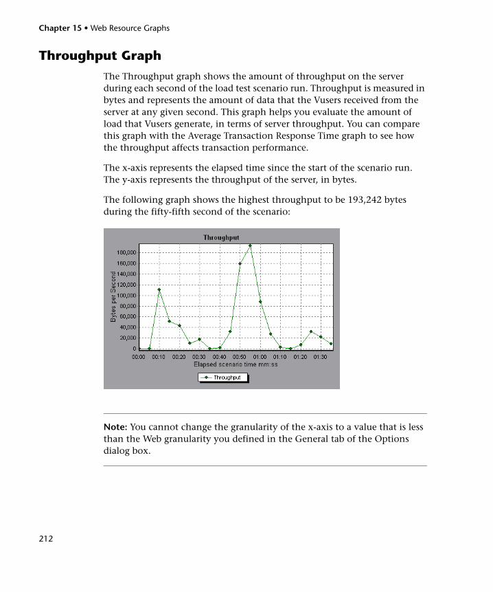
Chapter 15 • Web Resource Graphs
212
Throughput Graph
The Throughput graph shows the amount of throughput on the server during each second of the load test scenario run. Throughput is measured in bytes and represents the amount of data that the Vusers received from the server at any given second. This graph helps you evaluate the amount of load that Vusers generate, in terms of server throughput. You can compare this graph with the Average Transaction Response Time graph to see how the throughput affects transaction performance.
The x-axis represents the elapsed time since the start of the scenario run. The y-axis represents the throughput of the server, in bytes.
The following graph shows the highest throughput to be 193,242 bytes during the fifty-fifth second of the scenario:
Note: You cannot change the granularity of the x-axis to a value that is less than the Web granularity you defined in the General tab of the Options dialog box.
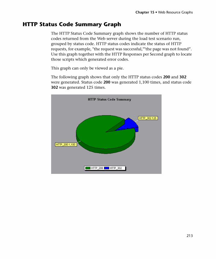
Chapter 15 • Web Resource Graphs
213
HTTP Status Code Summary Graph
The HTTP Status Code Summary graph shows the number of HTTP status codes returned from the Web server during the load test scenario run, grouped by status code. HTTP status codes indicate the status of HTTP requests, for example, "the request was successful,""the page was not found”. Use this graph together with the HTTP Responses per Second graph to locate those scripts which generated error codes.
This graph can only be viewed as a pie.
The following graph shows that only the HTTP status codes 200 and 302 were generated. Status code 200 was generated 1,100 times, and status code 302 was generated 125 times.
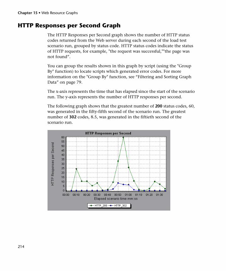
Chapter 15 • Web Resource Graphs
214
HTTP Responses per Second Graph
The HTTP Responses per Second graph shows the number of HTTP status codes returned from the Web server during each second of the load test scenario run, grouped by status code. HTTP status codes indicate the status of HTTP requests, for example, "the request was successful,""the page was not found”.
You can group the results shown in this graph by script (using the "Group By" function) to locate scripts which generated error codes. For more information on the "Group By" function, see “Filtering and Sorting Graph Data” on page 79.
The x-axis represents the time that has elapsed since the start of the scenario run. The y-axis represents the number of HTTP responses per second.
The following graph shows that the greatest number of 200 status codes, 60, was generated in the fifty-fifth second of the scenario run. The greatest number of 302 codes, 8.5, was generated in the fiftieth second of the scenario run.
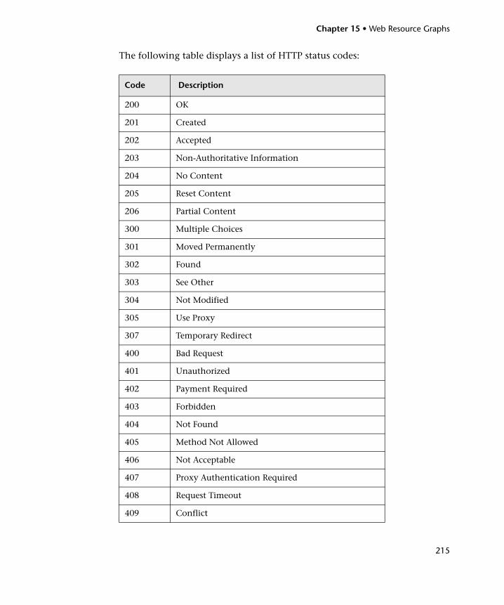
Chapter 15 • Web Resource Graphs
215
The following table displays a list of HTTP status codes:
Code Description
200 OK
201 Created
202 Accepted
203 Non-Authoritative Information
204 No Content
205 Reset Content
206 Partial Content
300 Multiple Choices
301 Moved Permanently
302 Found
303 See Other
304 Not Modified
305 Use Proxy
307 Temporary Redirect
400 Bad Request
401 Unauthorized
402 Payment Required
403 Forbidden
404 Not Found
405 Method Not Allowed
406 Not Acceptable
407 Proxy Authentication Required
408 Request Timeout
409 Conflict
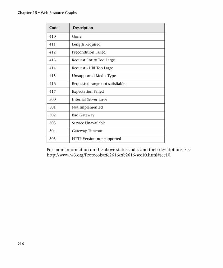
Chapter 15 • Web Resource Graphs
216
For more information on the above status codes and their descriptions, see http://www.w3.org/Protocols/rfc2616/rfc2616-sec10.html#sec10.
410 Gone
411 Length Required
412 Precondition Failed
413 Request Entity Too Large
414 Request - URI Too Large
415 Unsupported Media Type
416 Requested range not satisfiable
417 Expectation Failed
500 Internal Server Error
501 Not Implemented
502 Bad Gateway
503 Service Unavailable
504 Gateway Timeout
505 HTTP Version not supported
Code Description
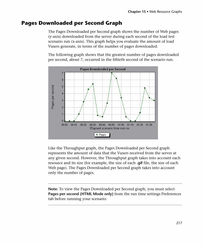
Chapter 15 • Web Resource Graphs
217
Pages Downloaded per Second Graph
The Pages Downloaded per Second graph shows the number of Web pages (y-axis) downloaded from the server during each second of the load test scenario run (x-axis). This graph helps you evaluate the amount of load Vusers generate, in terms of the number of pages downloaded.
The following graph shows that the greatest number of pages downloaded per second, about 7, occurred in the fiftieth second of the scenario run.
Like the Throughput graph, the Pages Downloaded per Second graph represents the amount of data that the Vusers received from the server at any given second. However, the Throughput graph takes into account each resource and its size (for example, the size of each .gif file, the size of each Web page). The Pages Downloaded per Second graph takes into account only the number of pages.
Note: To view the Pages Downloaded per Second graph, you must select Pages per second (HTML Mode only) from the run time settings Preferences tab before running your scenario.
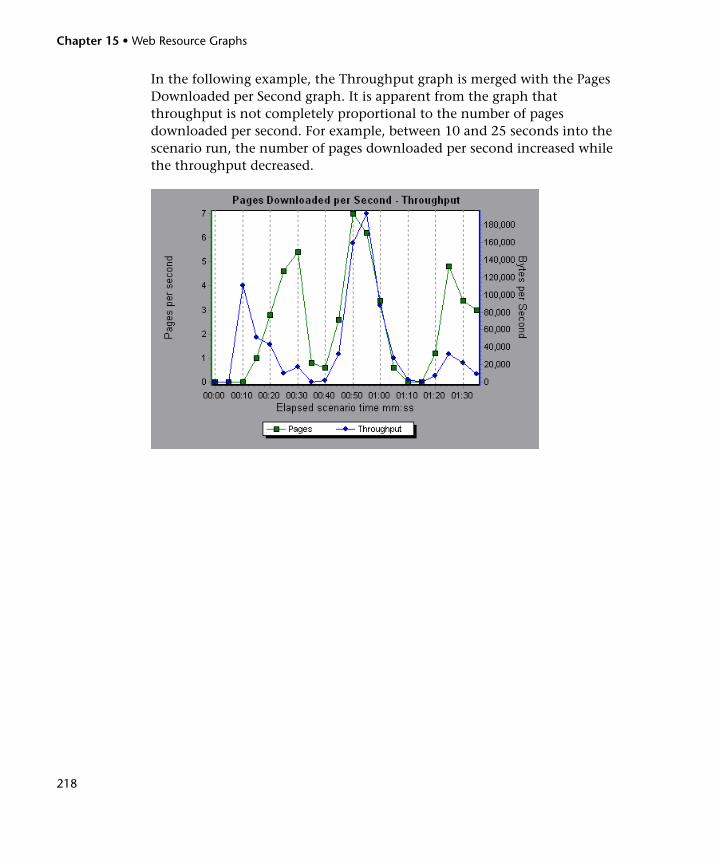
Chapter 15 • Web Resource Graphs
218
In the following example, the Throughput graph is merged with the Pages Downloaded per Second graph. It is apparent from the graph that throughput is not completely proportional to the number of pages downloaded per second. For example, between 10 and 25 seconds into the scenario run, the number of pages downloaded per second increased while the throughput decreased.
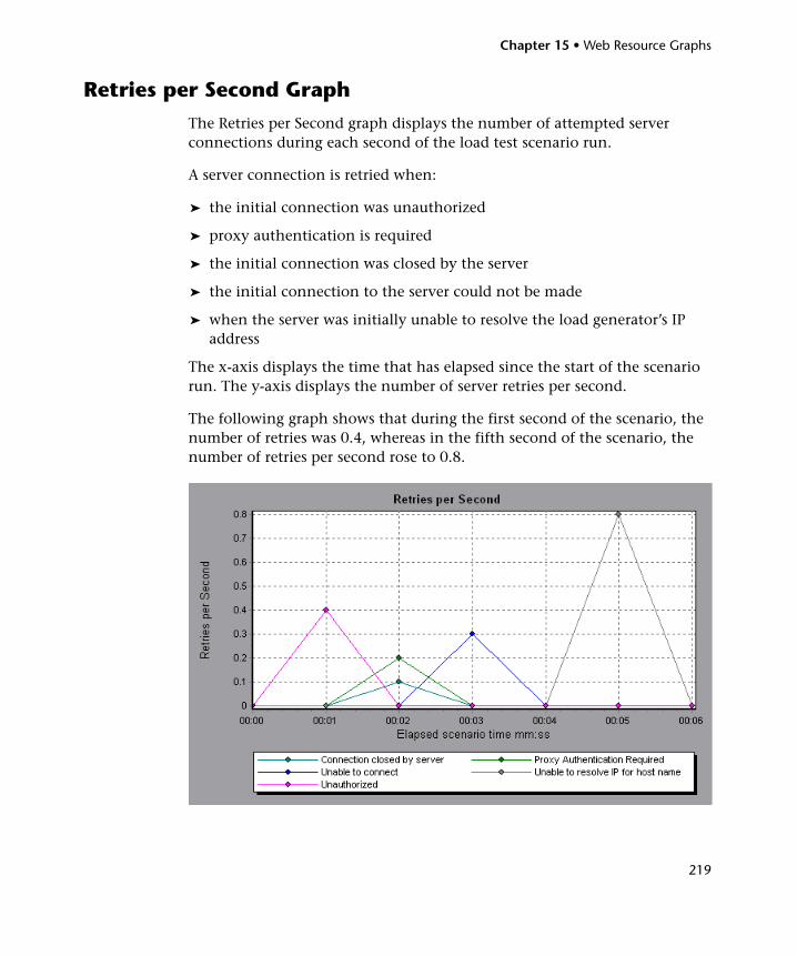
Chapter 15 • Web Resource Graphs
219
Retries per Second Graph
The Retries per Second graph displays the number of attempted server connections during each second of the load test scenario run.
A server connection is retried when:
➤ the initial connection was unauthorized
➤ proxy authentication is required
➤ the initial connection was closed by the server
➤ the initial connection to the server could not be made
➤ when the server was initially unable to resolve the load generator’s IP address
The x-axis displays the time that has elapsed since the start of the scenario run. The y-axis displays the number of server retries per second.
The following graph shows that during the first second of the scenario, the number of retries was 0.4, whereas in the fifth second of the scenario, the number of retries per second rose to 0.8.
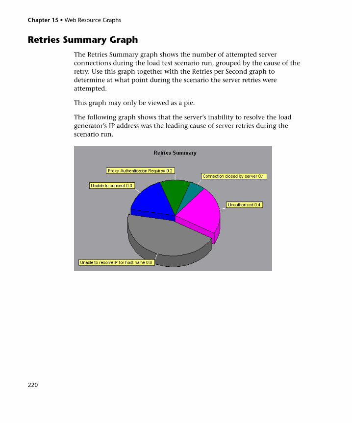
Chapter 15 • Web Resource Graphs
220
Retries Summary Graph
The Retries Summary graph shows the number of attempted server connections during the load test scenario run, grouped by the cause of the retry. Use this graph together with the Retries per Second graph to determine at what point during the scenario the server retries were attempted.
This graph may only be viewed as a pie.
The following graph shows that the server’s inability to resolve the load generator’s IP address was the leading cause of server retries during the scenario run.
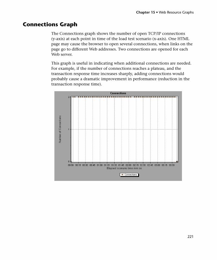
Chapter 15 • Web Resource Graphs
221
Connections Graph
The Connections graph shows the number of open TCP/IP connections (y-axis) at each point in time of the load test scenario (x-axis). One HTML page may cause the browser to open several connections, when links on the page go to different Web addresses. Two connections are opened for each Web server.
This graph is useful in indicating when additional connections are needed. For example, if the number of connections reaches a plateau, and the transaction response time increases sharply, adding connections would probably cause a dramatic improvement in performance (reduction in the transaction response time).
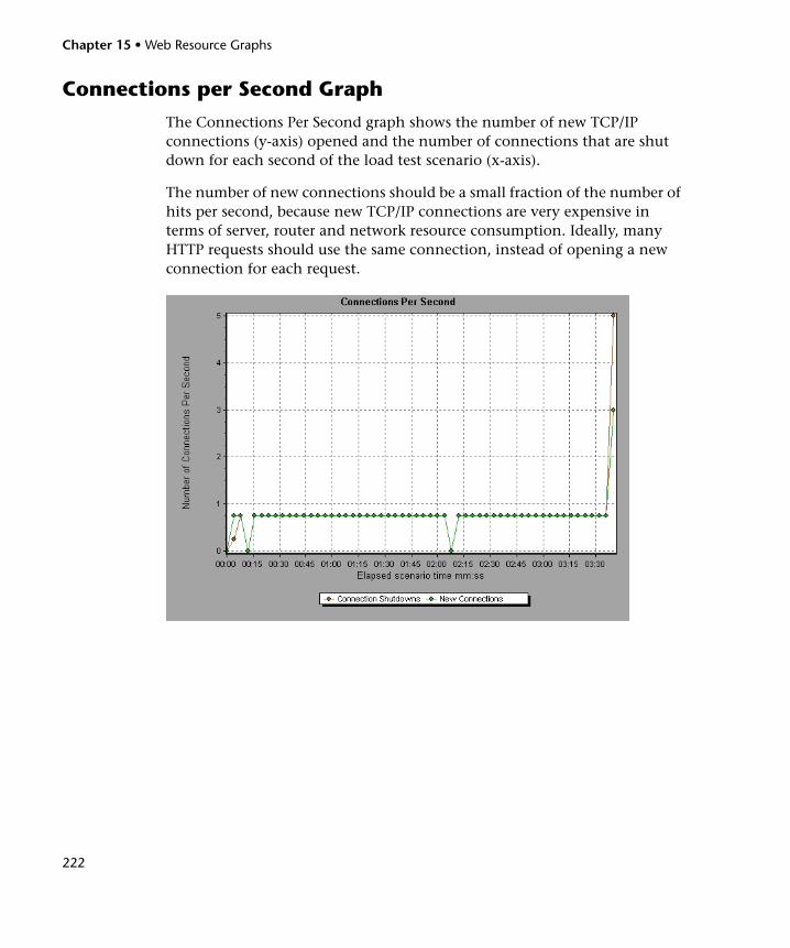
Chapter 15 • Web Resource Graphs
222
Connections per Second Graph
The Connections Per Second graph shows the number of new TCP/IP connections (y-axis) opened and the number of connections that are shut down for each second of the load test scenario (x-axis).
The number of new connections should be a small fraction of the number of hits per second, because new TCP/IP connections are very expensive in terms of server, router and network resource consumption. Ideally, many HTTP requests should use the same connection, instead of opening a new connection for each request.
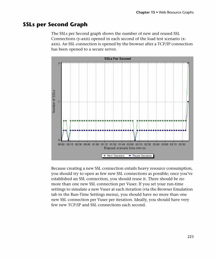
Chapter 15 • Web Resource Graphs
223
SSLs per Second Graph
The SSLs per Second graph shows the number of new and reused SSL Connections (y-axis) opened in each second of the load test scenario (x-axis). An SSL connection is opened by the browser after a TCP/IP connection has been opened to a secure server.
Because creating a new SSL connection entails heavy resource consumption, you should try to open as few new SSL connections as possible; once you’ve established an SSL connection, you should reuse it. There should be no more than one new SSL connection per Vuser. If you set your run-time settings to simulate a new Vuser at each iteration (via the Browser Emulation tab in the Run-Time Settings menu), you should have no more than one new SSL connection per Vuser per iteration. Ideally, you should have very few new TCP/IP and SSL connections each second.
Chapter 15 • Web Resource Graphs
224
225
16 Web Page Diagnostics Graphs
The Web Page Diagnostics graphs enable you to assess whether transaction response times were affected by page content. Using the Web Page Diagnostics graphs, you can analyze problematic elements—for example, images that download slowly, or broken links—of a Web site.
This chapter includes:
➤ About Web Page Diagnostics Graphs on page 226
➤ Activating the Web Page Diagnostics Graphs on page 228
➤ Page Component Breakdown Graph on page 231
➤ Page Component Breakdown (Over Time) Graph on page 233
➤ Page Download Time Breakdown Graph on page 235
➤ Page Download Time Breakdown (Over Time) Graph on page 239
➤ Time to First Buffer Breakdown Graph on page 241
➤ Time to First Buffer Breakdown (Over Time) Graph on page 243
➤ Downloaded Component Size Graph on page 245
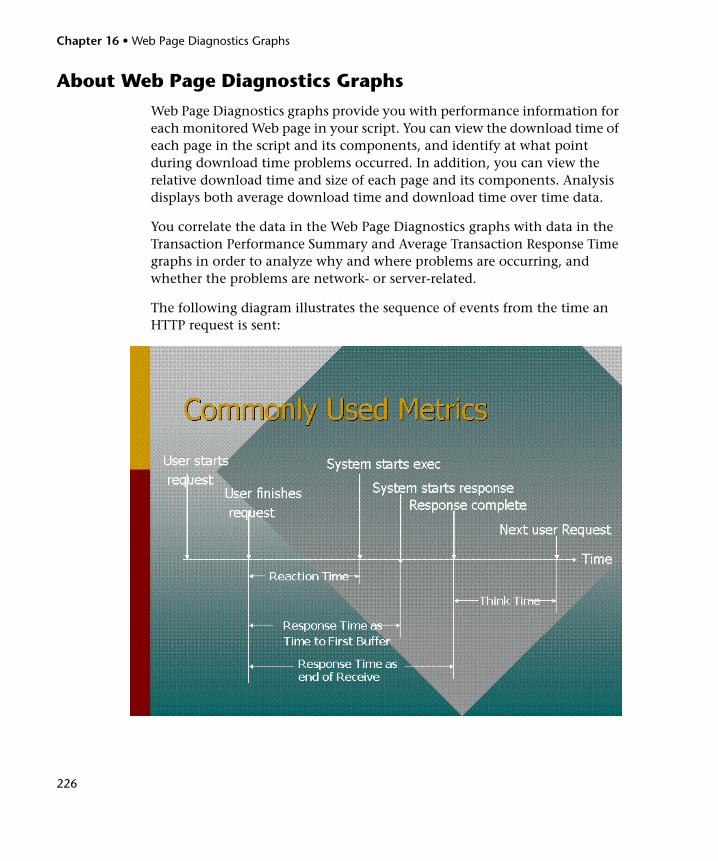
Chapter 16 • Web Page Diagnostics Graphs
226
About Web Page Diagnostics Graphs
Web Page Diagnostics graphs provide you with performance information for each monitored Web page in your script. You can view the download time of each page in the script and its components, and identify at what point during download time problems occurred. In addition, you can view the relative download time and size of each page and its components. Analysis displays both average download time and download time over time data.
You correlate the data in the Web Page Diagnostics graphs with data in the Transaction Performance Summary and Average Transaction Response Time graphs in order to analyze why and where problems are occurring, and whether the problems are network- or server-related.
The following diagram illustrates the sequence of events from the time an HTTP request is sent:
Chapter 16 • Web Page Diagnostics Graphs
227
Note: Because server time is being measured from the client, network time may influence this measurement if there is a change in network performance from the time the initial HTTP request is sent until the time the first buffer is sent. The server time displayed, therefore, is estimated server time and may be slightly inaccurate.
You begin analyzing the Transaction Performance Summary and Average Transaction Response Time graphs with the Web Page Diagnostics graph, which displays the average download time (in seconds) for each monitored Web page during each second of the load test scenario run. The x-axis represents the elapsed time from the beginning of the scenario run. The y-axis represents the average download time (in seconds) for each Web page.
In order for Analysis to generate Web Page Diagnostics graphs, you must enable the Web Page Diagnostics feature in the Controller before recording your script.
To enable the Web Page Diagnostics feature in the Controller:
1 From the Controller menu, choose Diagnostics > Configuration.
2 Select the Enable the following diagnostics check box.
3 Next to Web Page Diagnostics (Max. Vuser Sampling: 10%) click Enable.
4 Click OK.
Note: It is recommended that, in VuGen, you select HTML-based script in the Recording tab of the Recording Options dialog box.
For more information on recording Web Vuser scripts, refer to the HP Virtual User Generator User Guide.
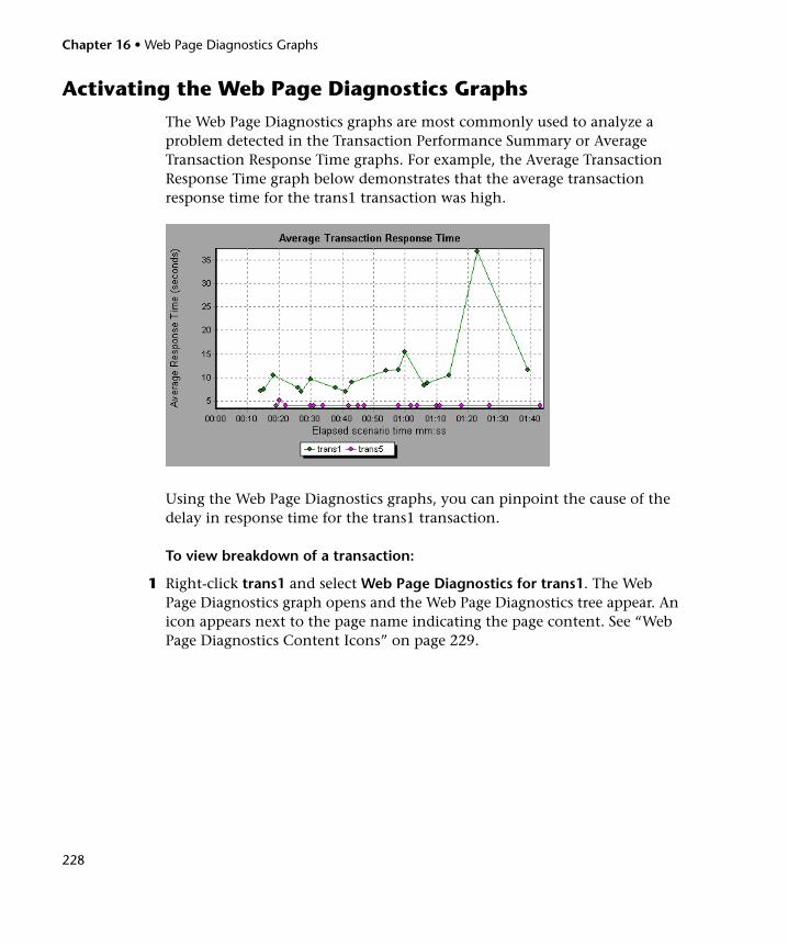
Chapter 16 • Web Page Diagnostics Graphs
228
Activating the Web Page Diagnostics Graphs
The Web Page Diagnostics graphs are most commonly used to analyze a problem detected in the Transaction Performance Summary or Average Transaction Response Time graphs. For example, the Average Transaction Response Time graph below demonstrates that the average transaction response time for the trans1 transaction was high.
Using the Web Page Diagnostics graphs, you can pinpoint the cause of the delay in response time for the trans1 transaction.
To view breakdown of a transaction:
1 Right-click trans1 and select Web Page Diagnostics for trans1. The Web Page Diagnostics graph opens and the Web Page Diagnostics tree appear. An icon appears next to the page name indicating the page content. See “Web Page Diagnostics Content Icons” on page 229.
Chapter 16 • Web Page Diagnostics Graphs
229
2 In the Web Page Diagnostics tree, right-click the problematic page you want to break down, and select Break Down <component name>. Alternatively, select a page in the Select Page to Break Down box that appears under the Web Page Diagnostics graph. The Web Page Diagnostics graph for that page appears.
Note: You can open a browser displaying the problematic page by right-clicking the page in the Web Page Diagnostics tree and selecting View page in browser.
3 Select one of the following available breakdown options:
➤ Download Time. Displays a table with a breakdown of the selected page’s download time. The size of each page component (including the component’s header) is displayed. See the “Page Download Time Breakdown Graph” on page 235 for more information about this display.
➤ Component (Over Time). Displays the Page Component Breakdown (Over Time) Graph for the selected Web page.
➤ Download Time (Over Time). Displays the Page Download Time Breakdown (Over Time) Graph for the selected Web page.
➤ Time to First Buffer (Over Time). Displays the Time to First Buffer Breakdown (Over Time) Graph for the selected Web page.
To display the graphs in full view, click the Enlarge Graph button. You can also access these graphs, as well as additional Web Page Diagnostics graphs, from the Open a New Graph dialog box.
Web Page Diagnostics Content Icons
The following icons appear in the Web Page Diagnostics tree. They indicate the HTTP content of the page.
Transaction. Specifies that the ensuing content is part of the transaction.
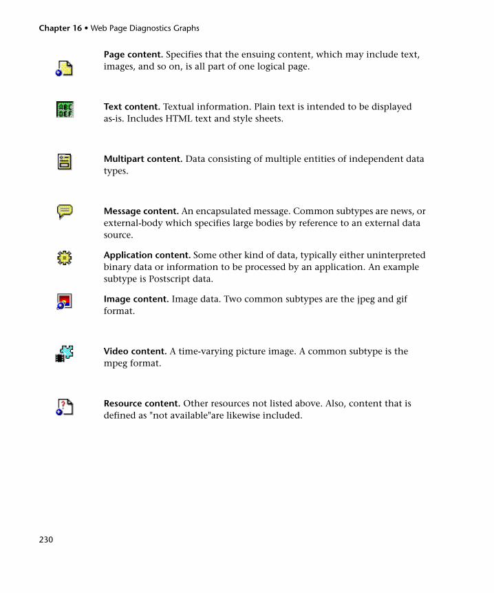
Chapter 16 • Web Page Diagnostics Graphs
230
Page content. Specifies that the ensuing content, which may include text, images, and so on, is all part of one logical page.
Text content. Textual information. Plain text is intended to be displayed as-is. Includes HTML text and style sheets.
Multipart content. Data consisting of multiple entities of independent data types.
Message content. An encapsulated message. Common subtypes are news, or external-body which specifies large bodies by reference to an external data source.
Application content. Some other kind of data, typically either uninterpreted binary data or information to be processed by an application. An example subtype is Postscript data.
Image content. Image data. Two common subtypes are the jpeg and gif format.
Video content. A time-varying picture image. A common subtype is the mpeg format.
Resource content. Other resources not listed above. Also, content that is defined as "not available"are likewise included.
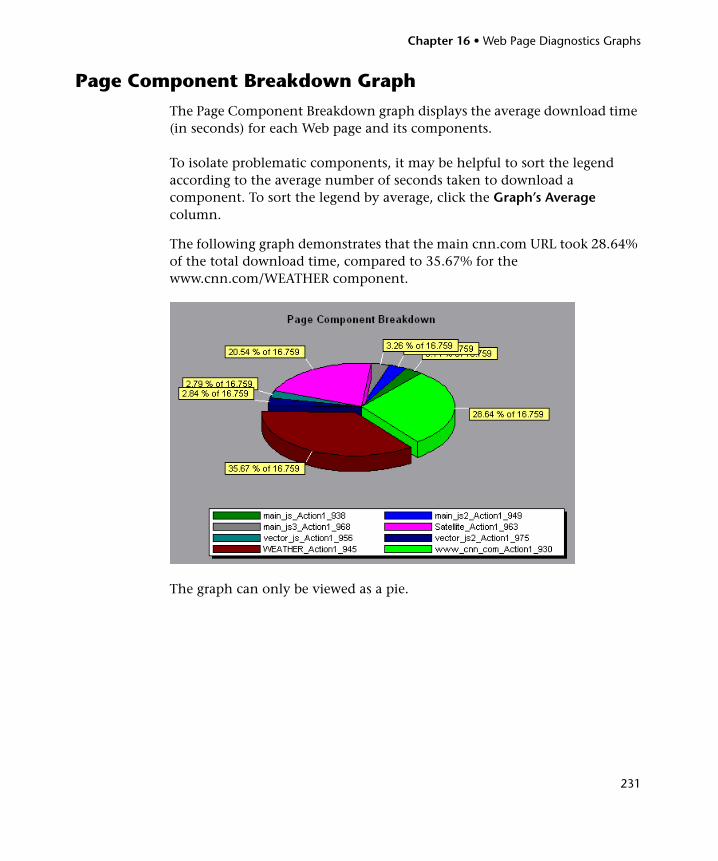
Chapter 16 • Web Page Diagnostics Graphs
231
Page Component Breakdown Graph
The Page Component Breakdown graph displays the average download time (in seconds) for each Web page and its components.
To isolate problematic components, it may be helpful to sort the legend according to the average number of seconds taken to download a component. To sort the legend by average, click the Graph’s Average column.
The following graph demonstrates that the main cnn.com URL took 28.64% of the total download time, compared to 35.67% for the www.cnn.com/WEATHER component.
The graph can only be viewed as a pie.
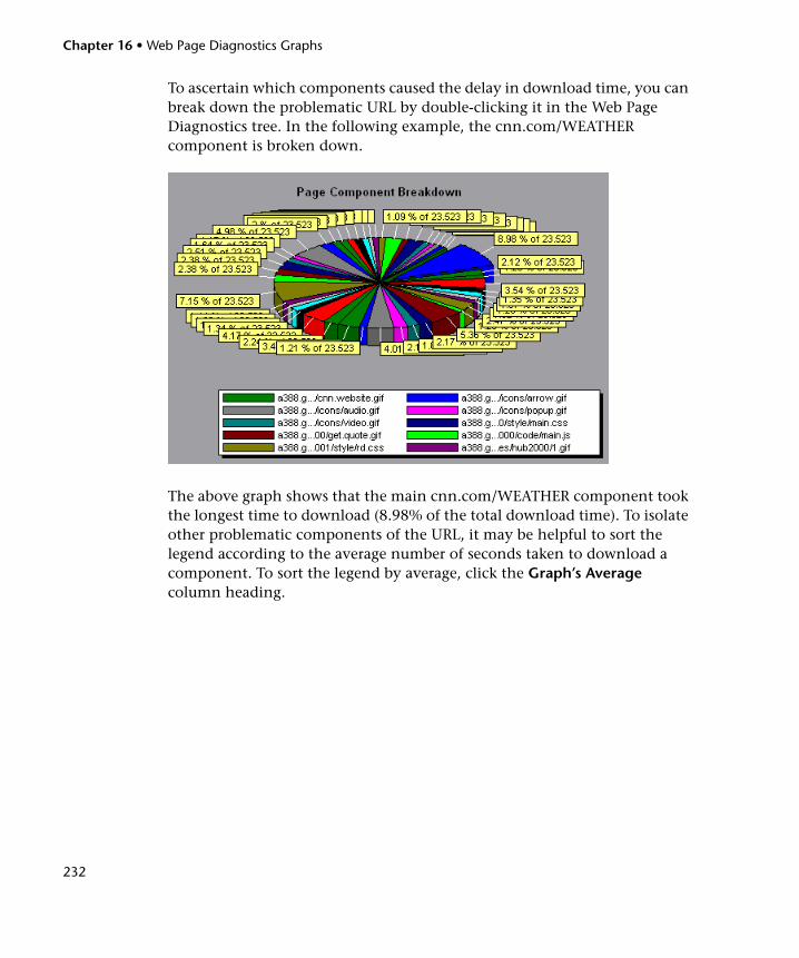
Chapter 16 • Web Page Diagnostics Graphs
232
To ascertain which components caused the delay in download time, you can break down the problematic URL by double-clicking it in the Web Page Diagnostics tree. In the following example, the cnn.com/WEATHER component is broken down.
The above graph shows that the main cnn.com/WEATHER component took the longest time to download (8.98% of the total download time). To isolate other problematic components of the URL, it may be helpful to sort the legend according to the average number of seconds taken to download a component. To sort the legend by average, click the Graph’s Average column heading.
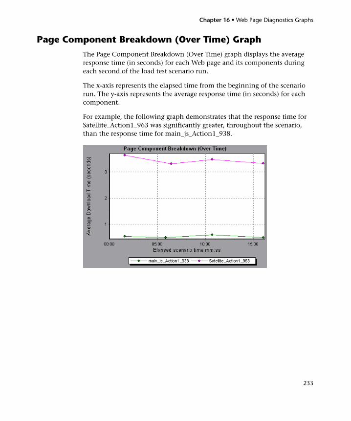
Chapter 16 • Web Page Diagnostics Graphs
233
Page Component Breakdown (Over Time) Graph
The Page Component Breakdown (Over Time) graph displays the average response time (in seconds) for each Web page and its components during each second of the load test scenario run.
The x-axis represents the elapsed time from the beginning of the scenario run. The y-axis represents the average response time (in seconds) for each component.
For example, the following graph demonstrates that the response time for Satellite_Action1_963 was significantly greater, throughout the scenario, than the response time for main_js_Action1_938.
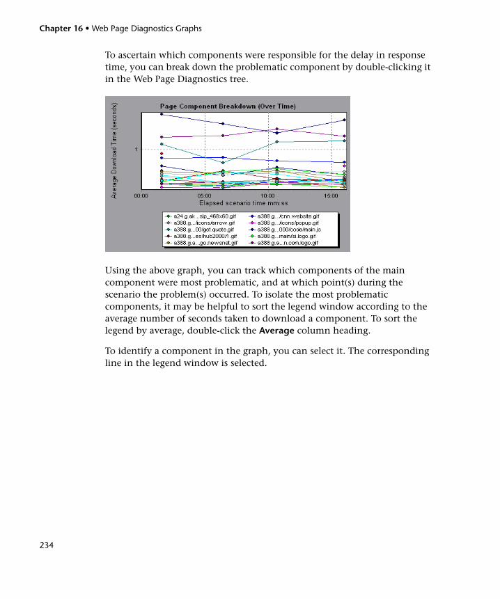
Chapter 16 • Web Page Diagnostics Graphs
234
To ascertain which components were responsible for the delay in response time, you can break down the problematic component by double-clicking it in the Web Page Diagnostics tree.
Using the above graph, you can track which components of the main component were most problematic, and at which point(s) during the scenario the problem(s) occurred. To isolate the most problematic components, it may be helpful to sort the legend window according to the average number of seconds taken to download a component. To sort the legend by average, double-click the Average column heading.
To identify a component in the graph, you can select it. The corresponding line in the legend window is selected.
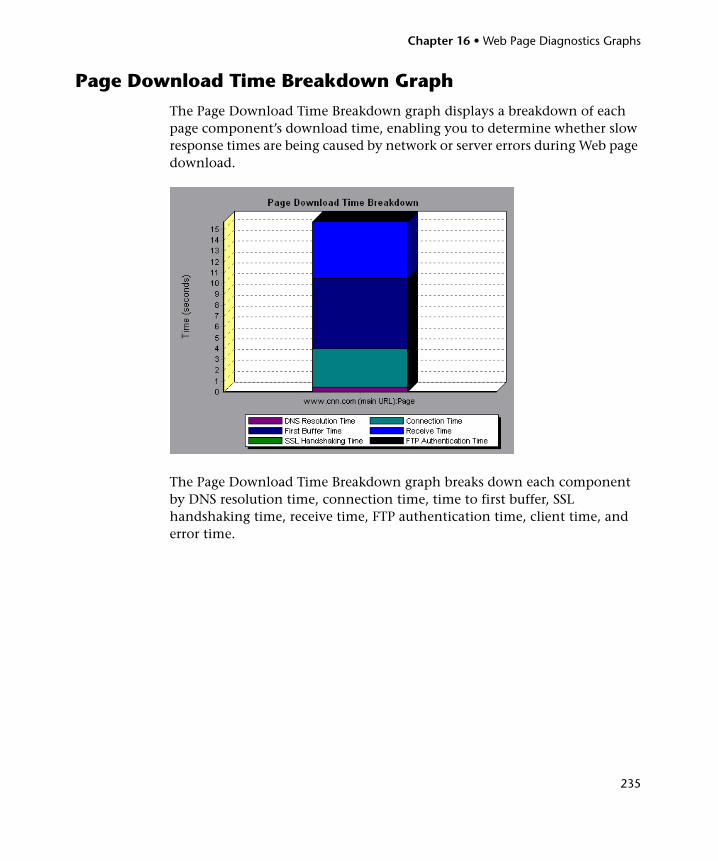
Chapter 16 • Web Page Diagnostics Graphs
235
Page Download Time Breakdown Graph
The Page Download Time Breakdown graph displays a breakdown of each page component’s download time, enabling you to determine whether slow response times are being caused by network or server errors during Web page download.
The Page Download Time Breakdown graph breaks down each component by DNS resolution time, connection time, time to first buffer, SSL handshaking time, receive time, FTP authentication time, client time, and error time.
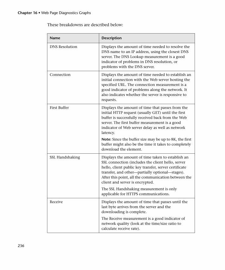
Chapter 16 • Web Page Diagnostics Graphs
236
These breakdowns are described below:
Name Description
DNS Resolution Displays the amount of time needed to resolve the DNS name to an IP address, using the closest DNS server. The DNS Lookup measurement is a good indicator of problems in DNS resolution, or problems with the DNS server.
Connection Displays the amount of time needed to establish an initial connection with the Web server hosting the specified URL. The connection measurement is a good indicator of problems along the network. It also indicates whether the server is responsive to requests.
First Buffer Displays the amount of time that passes from the initial HTTP request (usually GET) until the first buffer is successfully received back from the Web server. The first buffer measurement is a good indicator of Web server delay as well as network latency.
Note: Since the buffer size may be up to 8K, the first buffer might also be the time it takes to completely download the element.
SSL Handshaking Displays the amount of time taken to establish an SSL connection (includes the client hello, server hello, client public key transfer, server certificate transfer, and other—partially optional—stages). After this point, all the communication between the client and server is encrypted.
The SSL Handshaking measurement is only applicable for HTTPS communications.
Receive Displays the amount of time that passes until the last byte arrives from the server and the downloading is complete.
The Receive measurement is a good indicator of network quality (look at the time/size ratio to calculate receive rate).
Chapter 16 • Web Page Diagnostics Graphs
237
Note: Each measurement displayed on the page level is the sum of that measurement recorded for each page component. For example, the Connection Time for www.cnn.com is the sum of the Connection Time for each of the page’s components.
The Page Download Time Breakdown graph on page 235 demonstrates that receive time, connection time, and first buffer time accounted for a large portion of the time taken to download the main cnn.com URL.
FTP Authentication Displays the time taken to authenticate the client. With FTP, a server must authenticate a client before it starts processing the client’s commands.
The FTP Authentication measurement is only applicable for FTP protocol communications.
Client Time Displays the average amount of time that passes while a request is delayed on the client machine due to browser think time or other client-related delays.
Error Time Displays the average amount of time that passes from the moment an HTTP request is sent until the moment an error message (HTTP errors only) is returned.
Name Description
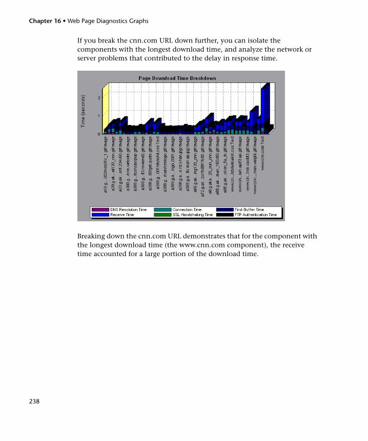
Chapter 16 • Web Page Diagnostics Graphs
238
If you break the cnn.com URL down further, you can isolate the components with the longest download time, and analyze the network or server problems that contributed to the delay in response time.
Breaking down the cnn.com URL demonstrates that for the component with the longest download time (the www.cnn.com component), the receive time accounted for a large portion of the download time.
Chapter 16 • Web Page Diagnostics Graphs
239
Page Download Time Breakdown (Over Time) Graph
The Page Download Time Breakdown (Over Time) graph displays a breakdown of each page component’s download time during each second of the load test scenario run.
The x-axis represents the elapsed time from the beginning of the scenario run. The y-axis represents the time (in seconds) taken for each step in the download process.
This graph enables you to determine at what point during scenario execution network or server problems occurred.
Note: Each measurement displayed on the page level is the sum of that measurement recorded for each page component. For example, the Connection Time for www.cnn.com is the sum of the Connection Time for each of the page’s components.
To isolate the most problematic components, you can sort the legend window according to the average number of seconds taken to download a component. To sort the legend by average, double-click the Average column heading.
Chapter 16 • Web Page Diagnostics Graphs
240
To identify a component in the graph, select it. The corresponding line in the legend window is selected.
In the example in the previous section, it is apparent that cnn.com was the most problematic component. If you examine the cnn.com component, the Page Download Time Breakdown (Over Time) graph demonstrates that First Buffer and Receive time remained high throughout the scenario, and that DNS Resolution time decreased during the scenario.
Note: When the Page Download Time Breakdown (Over Time) graph is selected from the Web Page Diagnostics graph, it appears as an area graph.
Chapter 16 • Web Page Diagnostics Graphs
241
Time to First Buffer Breakdown Graph
The Time to First Buffer Breakdown graph displays each Web page component’s relative server/network time (in seconds) for the period of time until the first buffer is successfully received back from the Web server. If the download time for a component is high, you can use this graph to determine whether the problem is server- or network-related.
The x-axis specifies the name of the component. The y-axis shows the average network/server time (in seconds) for each component.
Note: Each measurement displayed on the page level is the sum of that measurement recorded for each page component. For example, the network time for www.cnn.com is the sum of the network time for each of the page’s components.
Network time is defined as the average amount of time that passes from the moment the first HTTP request is sent until receipt of ACK.
Server time is defined as the average amount of time that passes from the receipt of ACK of the initial HTTP request (usually GET) until the first buffer is successfully received back from the Web server.
Chapter 16 • Web Page Diagnostics Graphs
242
In the above graph, it is apparent that network time is greater than server time.
Note: Because server time is being measured from the client, network time may influence this measurement if there is a change in network performance from the time the initial HTTP request is sent until the time the first buffer is sent. The server time displayed, therefore, is estimated server time and may be slightly inaccurate.
The graph can only be viewed as a bar graph.
You can break the main cnn.com URL down further to view the time to first buffer breakdown for each of its components.
It is apparent that for the main cnn.com component (the first component on the right), the time to first buffer breakdown is almost all network time.
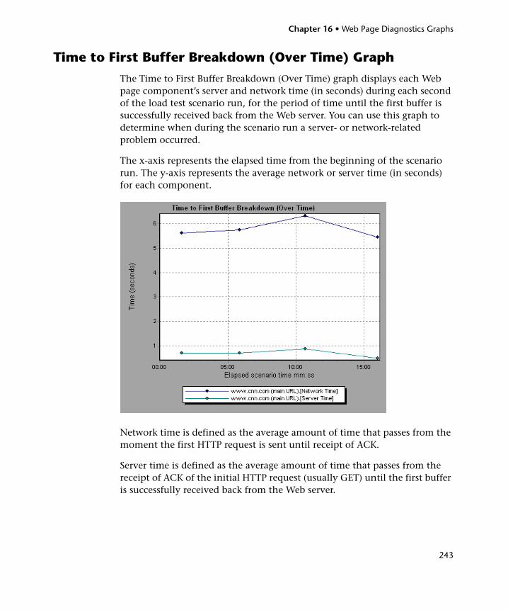
Chapter 16 • Web Page Diagnostics Graphs
243
Time to First Buffer Breakdown (Over Time) Graph
The Time to First Buffer Breakdown (Over Time) graph displays each Web page component’s server and network time (in seconds) during each second of the load test scenario run, for the period of time until the first buffer is successfully received back from the Web server. You can use this graph to determine when during the scenario run a server- or network-related problem occurred.
The x-axis represents the elapsed time from the beginning of the scenario run. The y-axis represents the average network or server time (in seconds) for each component.
Network time is defined as the average amount of time that passes from the moment the first HTTP request is sent until receipt of ACK.
Server time is defined as the average amount of time that passes from the receipt of ACK of the initial HTTP request (usually GET) until the first buffer is successfully received back from the Web server.
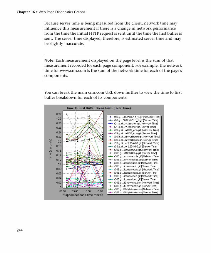
Chapter 16 • Web Page Diagnostics Graphs
244
Because server time is being measured from the client, network time may influence this measurement if there is a change in network performance from the time the initial HTTP request is sent until the time the first buffer is sent. The server time displayed, therefore, is estimated server time and may be slightly inaccurate.
Note: Each measurement displayed on the page level is the sum of that measurement recorded for each page component. For example, the network time for www.cnn.com is the sum of the network time for each of the page’s components.
You can break the main cnn.com URL down further to view the time to first buffer breakdown for each of its components.
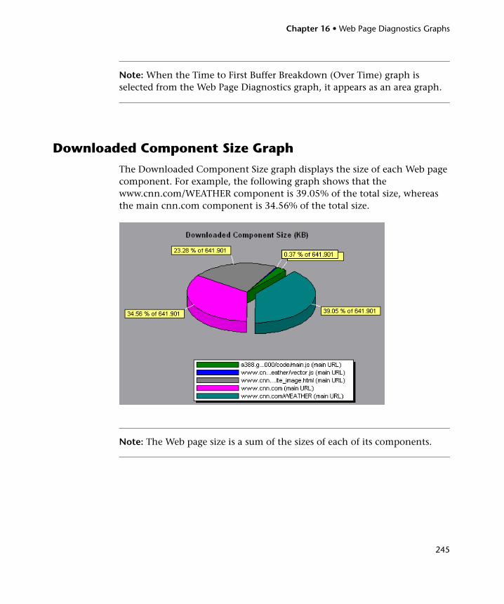
Chapter 16 • Web Page Diagnostics Graphs
245
Note: When the Time to First Buffer Breakdown (Over Time) graph is selected from the Web Page Diagnostics graph, it appears as an area graph.
Downloaded Component Size Graph
The Downloaded Component Size graph displays the size of each Web page component. For example, the following graph shows that the www.cnn.com/WEATHER component is 39.05% of the total size, whereas the main cnn.com component is 34.56% of the total size.
Note: The Web page size is a sum of the sizes of each of its components.
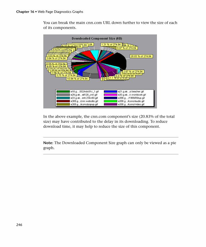
Chapter 16 • Web Page Diagnostics Graphs
246
You can break the main cnn.com URL down further to view the size of each of its components.
In the above example, the cnn.com component’s size (20.83% of the total size) may have contributed to the delay in its downloading. To reduce download time, it may help to reduce the size of this component.
Note: The Downloaded Component Size graph can only be viewed as a pie graph.
247
17 User-Defined Data Point Graphs
After a load test scenario run, you can use the User-Defined Data Point graphs to display the values of user-defined data points in the Vuser script.
This chapter includes:
➤ About User-Defined Data Point Graphs on page 247
➤ Data Points (Sum) Graph on page 248
➤ Data Points (Average) Graph on page 250
About User-Defined Data Point Graphs
The User-Defined Data Point graphs display the values of user-defined data points. You define a data point in your Vuser script by inserting an lr_user_data_point function at the appropriate place (user_data_point for GUI Vusers and lr.user_data_point for Java Vusers).
Action1(){lr_think_time(1);lr_user_data_point ("data_point_1",1);lr_user_data_point ("data_point_2",2);return 0;
}

Chapter 17 • User-Defined Data Point Graphs
248
For Vuser protocols that support the graphical script representations such as Web and Oracle NCA, you insert a data point as a User Defined step. Data point information is gathered each time the script executes the function or step. For more information about data points, refer to the online HP LoadRunner Online Function Reference.
Data points, like other Analysis data, are aggregated every few seconds, resulting in less data points shown on the graph than actually recorded. For more information see, “Changing the Granularity of the Data” on page 105.
Data Points (Sum) Graph
The Data Points (Sum) graph shows the sum of the values for user-defined data points throughout the load test scenario run.
The x-axis represents the number of seconds that elapsed since the start time of the run. The y-axis displays the sum of the recorded data point values.
This graph typically indicates the total amount of measurements which all Virtual Users are able to generate. For example, suppose only a certain set of circumstances allow a Vuser to call a server. Each time it does, a data point is recorded. In this case, the Sum graph displays the total number of times that Vusers call the function.
Chapter 17 • User-Defined Data Point Graphs
249
In the following example, the call to the server is recorded as the data point user_data_point_val_1. It is shown as a function of the elapsed scenario time.
Chapter 17 • User-Defined Data Point Graphs
250
Data Points (Average) Graph
The Data Points (Average) graph shows the average values that were recorded for user-defined data points during the load test scenario run.
The x-axis represents the number of seconds that elapsed since the start time of the run. The y-axis displays the average values of the recorded data point statements.
This graph is typically used in cases where the actual value of the measurement is required. Suppose that each Vuser monitors CPU utilization on its machine and records it as a data point. In this case, the actual recorded value of CPU utilization is required. The Average graph displays the average value recorded throughout the scenario.
In the following example, the CPU utilization is recorded as the data point user_data_point_val_1. It is shown as a function of the elapsed scenario time:
251
18 System Resource Graphs
After running a load test scenario, you can check the various system resources that were monitored during the scenario.
This chapter includes:
➤ About System Resource Graphs on page 251
➤ Windows Resources Graph on page 252
➤ UNIX Resources Graph on page 256
➤ Server Resources Graph on page 258
➤ SNMP Resources Graph on page 260
➤ Antara FlameThrower Resources Graph on page 261
➤ SiteScope Graph on page 273
About System Resource Graphs
System Resource graphs display the system resource usage measured by the online monitors during the load test scenario run. These graphs require that you specify the resources you want to measure before running the scenario. For more information, refer to the section on online monitors in the HP LoadRunner Controller User Guide.
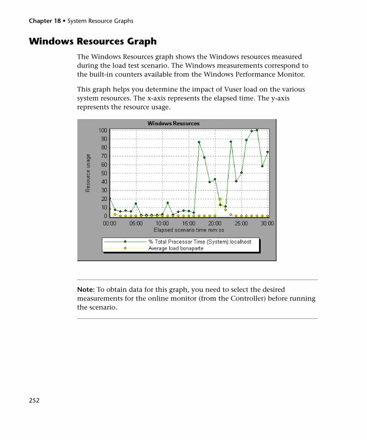
Chapter 18 • System Resource Graphs
252
Windows Resources Graph
The Windows Resources graph shows the Windows resources measured during the load test scenario. The Windows measurements correspond to the built-in counters available from the Windows Performance Monitor.
This graph helps you determine the impact of Vuser load on the various system resources. The x-axis represents the elapsed time. The y-axis represents the resource usage.
Note: To obtain data for this graph, you need to select the desired measurements for the online monitor (from the Controller) before running the scenario.
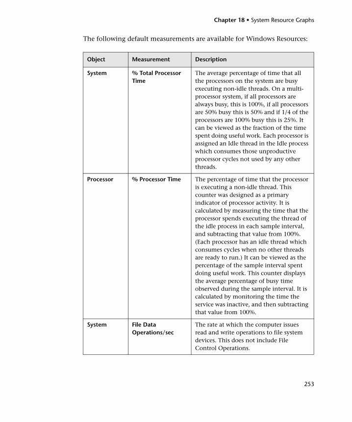
Chapter 18 • System Resource Graphs
253
The following default measurements are available for Windows Resources:
Object Measurement Description
System % Total Processor Time
The average percentage of time that all the processors on the system are busy executing non-idle threads. On a multi-processor system, if all processors are always busy, this is 100%, if all processors are 50% busy this is 50% and if 1/4 of the processors are 100% busy this is 25%. It can be viewed as the fraction of the time spent doing useful work. Each processor is assigned an Idle thread in the Idle process which consumes those unproductive processor cycles not used by any other threads.
Processor % Processor Time The percentage of time that the processor is executing a non-idle thread. This counter was designed as a primary indicator of processor activity. It is calculated by measuring the time that the processor spends executing the thread of the idle process in each sample interval, and subtracting that value from 100%. (Each processor has an idle thread which consumes cycles when no other threads are ready to run.) It can be viewed as the percentage of the sample interval spent doing useful work. This counter displays the average percentage of busy time observed during the sample interval. It is calculated by monitoring the time the service was inactive, and then subtracting that value from 100%.
System File Data Operations/sec
The rate at which the computer issues read and write operations to file system devices. This does not include File Control Operations.
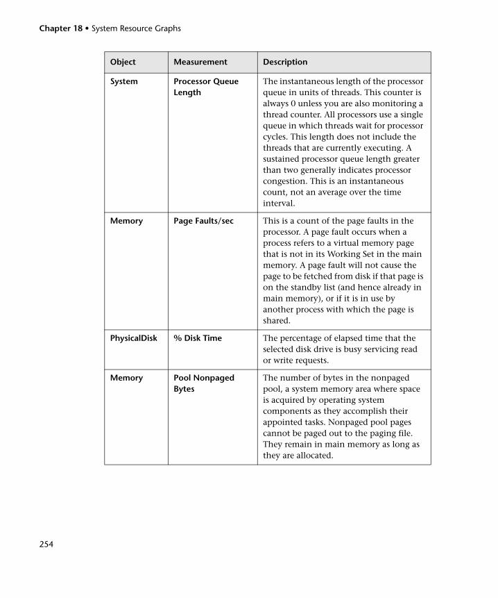
Chapter 18 • System Resource Graphs
254
System Processor Queue Length
The instantaneous length of the processor queue in units of threads. This counter is always 0 unless you are also monitoring a thread counter. All processors use a single queue in which threads wait for processor cycles. This length does not include the threads that are currently executing. A sustained processor queue length greater than two generally indicates processor congestion. This is an instantaneous count, not an average over the time interval.
Memory Page Faults/sec This is a count of the page faults in the processor. A page fault occurs when a process refers to a virtual memory page that is not in its Working Set in the main memory. A page fault will not cause the page to be fetched from disk if that page is on the standby list (and hence already in main memory), or if it is in use by another process with which the page is shared.
PhysicalDisk % Disk Time The percentage of elapsed time that the selected disk drive is busy servicing read or write requests.
Memory Pool Nonpaged Bytes
The number of bytes in the nonpaged pool, a system memory area where space is acquired by operating system components as they accomplish their appointed tasks. Nonpaged pool pages cannot be paged out to the paging file. They remain in main memory as long as they are allocated.
Object Measurement Description
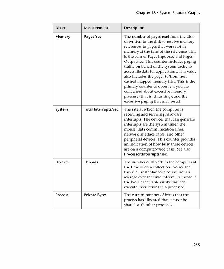
Chapter 18 • System Resource Graphs
255
Memory Pages/sec The number of pages read from the disk or written to the disk to resolve memory references to pages that were not in memory at the time of the reference. This is the sum of Pages Input/sec and Pages Output/sec. This counter includes paging traffic on behalf of the system cache to access file data for applications. This value also includes the pages to/from non-cached mapped memory files. This is the primary counter to observe if you are concerned about excessive memory pressure (that is, thrashing), and the excessive paging that may result.
System Total Interrupts/sec The rate at which the computer is receiving and servicing hardware interrupts. The devices that can generate interrupts are the system timer, the mouse, data communication lines, network interface cards, and other peripheral devices. This counter provides an indication of how busy these devices are on a computer-wide basis. See also Processor:Interrupts/sec.
Objects Threads The number of threads in the computer at the time of data collection. Notice that this is an instantaneous count, not an average over the time interval. A thread is the basic executable entity that can execute instructions in a processor.
Process Private Bytes The current number of bytes that the process has allocated that cannot be shared with other processes.
Object Measurement Description
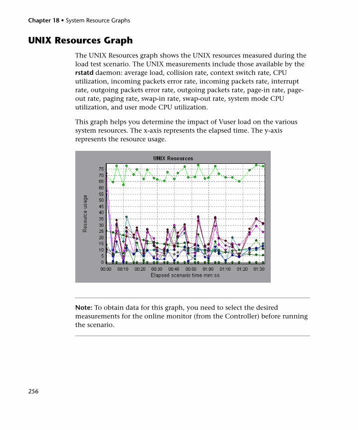
Chapter 18 • System Resource Graphs
256
UNIX Resources Graph
The UNIX Resources graph shows the UNIX resources measured during the load test scenario. The UNIX measurements include those available by the rstatd daemon: average load, collision rate, context switch rate, CPU utilization, incoming packets error rate, incoming packets rate, interrupt rate, outgoing packets error rate, outgoing packets rate, page-in rate, page-out rate, paging rate, swap-in rate, swap-out rate, system mode CPU utilization, and user mode CPU utilization.
This graph helps you determine the impact of Vuser load on the various system resources. The x-axis represents the elapsed time. The y-axis represents the resource usage.
Note: To obtain data for this graph, you need to select the desired measurements for the online monitor (from the Controller) before running the scenario.
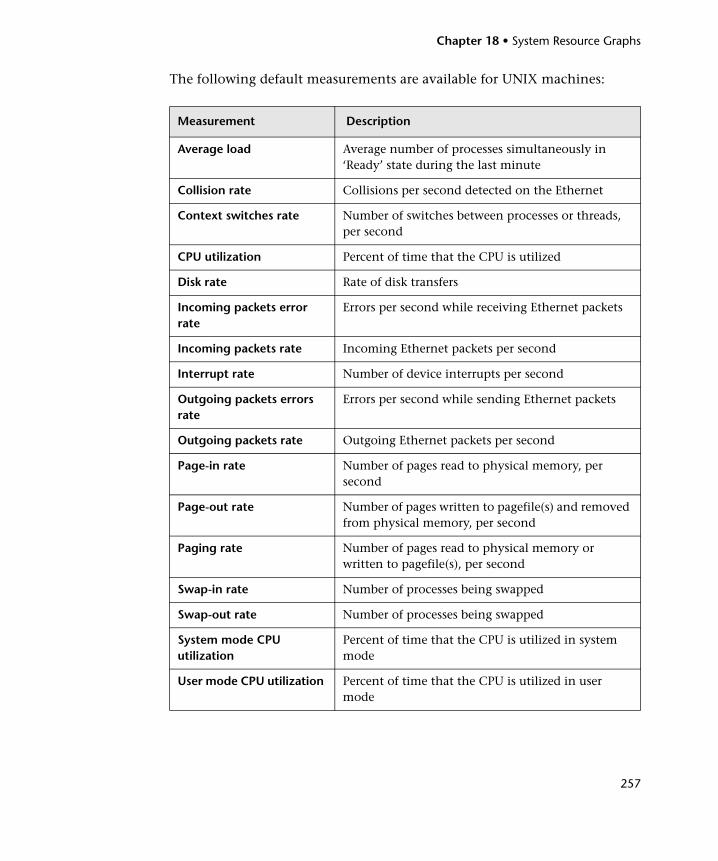
Chapter 18 • System Resource Graphs
257
The following default measurements are available for UNIX machines:
Measurement Description
Average load Average number of processes simultaneously in ‘Ready’ state during the last minute
Collision rate Collisions per second detected on the Ethernet
Context switches rate Number of switches between processes or threads, per second
CPU utilization Percent of time that the CPU is utilized
Disk rate Rate of disk transfers
Incoming packets error rate
Errors per second while receiving Ethernet packets
Incoming packets rate Incoming Ethernet packets per second
Interrupt rate Number of device interrupts per second
Outgoing packets errors rate
Errors per second while sending Ethernet packets
Outgoing packets rate Outgoing Ethernet packets per second
Page-in rate Number of pages read to physical memory, per second
Page-out rate Number of pages written to pagefile(s) and removed from physical memory, per second
Paging rate Number of pages read to physical memory or written to pagefile(s), per second
Swap-in rate Number of processes being swapped
Swap-out rate Number of processes being swapped
System mode CPU utilization
Percent of time that the CPU is utilized in system mode
User mode CPU utilization Percent of time that the CPU is utilized in user mode
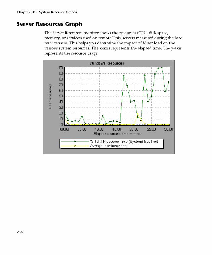
Chapter 18 • System Resource Graphs
258
Server Resources Graph
The Server Resources monitor shows the resources (CPU, disk space, memory, or services) used on remote Unix servers measured during the load test scenario. This helps you determine the impact of Vuser load on the various system resources. The x-axis represents the elapsed time. The y-axis represents the resource usage.
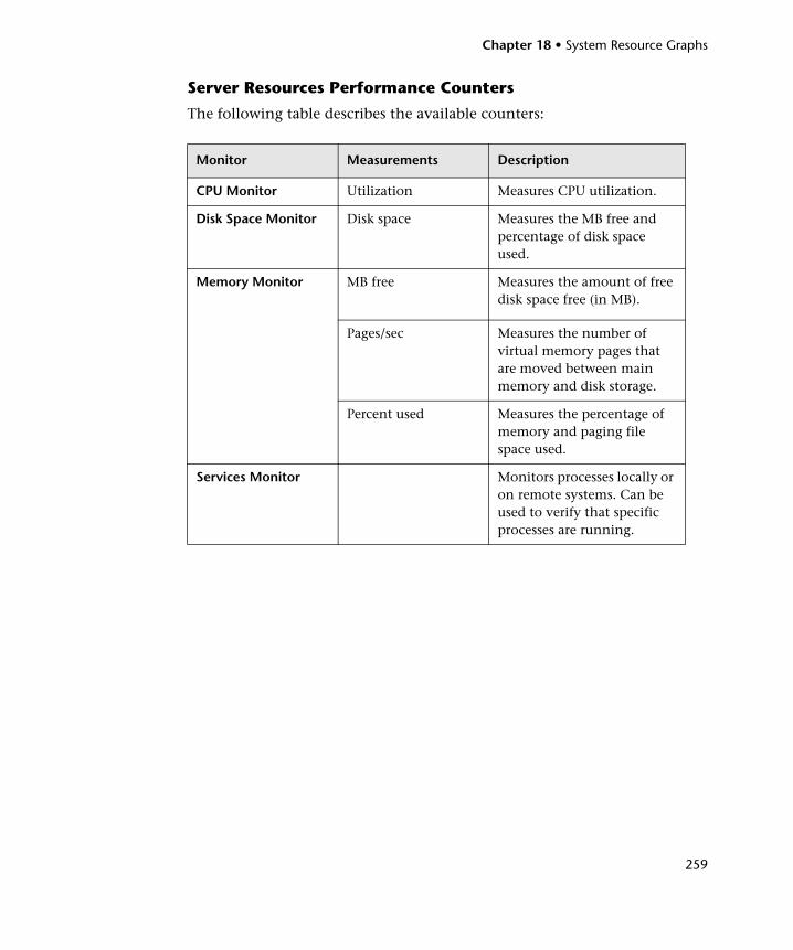
Chapter 18 • System Resource Graphs
259
Server Resources Performance Counters
The following table describes the available counters:
Monitor Measurements Description
CPU Monitor Utilization Measures CPU utilization.
Disk Space Monitor Disk space Measures the MB free and percentage of disk space used.
Memory Monitor MB free Measures the amount of free disk space free (in MB).
Pages/sec Measures the number of virtual memory pages that are moved between main memory and disk storage.
Percent used Measures the percentage of memory and paging file space used.
Services Monitor Monitors processes locally or on remote systems. Can be used to verify that specific processes are running.
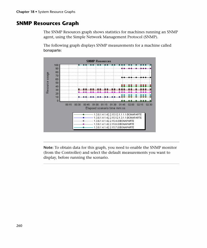
Chapter 18 • System Resource Graphs
260
SNMP Resources Graph
The SNMP Resources graph shows statistics for machines running an SNMP agent, using the Simple Network Management Protocol (SNMP).
The following graph displays SNMP measurements for a machine called bonaparte:
Note: To obtain data for this graph, you need to enable the SNMP monitor (from the Controller) and select the default measurements you want to display, before running the scenario.
Chapter 18 • System Resource Graphs
261
Antara FlameThrower Resources Graph
The Antara FlameThrower graph displays statistics about the resource usage on the Antara FlameThrower server during the load test scenario run.
The x-axis represents the time that has elapsed since the start of the scenario run. The y-axis represents the resource usage.
Note: To obtain data for this graph, you need to enable the iPlanet/Netscape online monitor (from the Controller) and select the default measurements you want to display, before running the scenario.
The following default measurements are available for the Antara FlameThrower server:
Layer Performance Counters
The following counters measure Layer performance:
Measurement Description
TxBytes The total number of Layer 2 data bytes transmitted.
TxByteRate(/sec) The number of Layer 2 data bytes transmitted per second.
TxFrames The total number of packets transmitted.
TxFrameRate(/sec) The number of packets transmitted per second.
RxBytes The total number of Layer 2 data bytes received.
RxByteRate(/sec) The number of Layer 2 data bytes received per second.
RxFrames The total number of packets received.
RxFrameRate(/sec) The number of packets received per second.
Chapter 18 • System Resource Graphs
262
TCP Performance Counters
The following counters measure TCP performance:
Measurement Description
ActiveTCPConns Total number of currently active TCP connections.
SuccTCPConns Total number of SYN ACK packets received.
SuccTCPConnRate(/sec)
Number of SYN ACK packets received per second.
TCPConnLatency(milisec)
Interval between transmitting a SYN packet and receiving a SYN ACK reply packet in msec.
MinTCPConnLatency(milisec)
Minimum TCPConnectionLatency in msec.
MaxTCPConnLatency(milisec)
Maximum TCPConnectionLatency in msec.
TCPSndConnClose Total number of FIN or FIN ACK packets transmitted (Client).
TCPRcvConnClose Total number of FIN or FIN ACK packets received (Client).
TCPSndResets Total number of RST packets transmitted.
TCPRcvResets Total number of RST packets received.
SYNSent Total number of SYN packets transmitted.
SYNSentRate(/sec) Number of SYN packets transmitted per second.
SYNAckSent Total number of SYN ACK packets transmitted.
SYNAckRate(/sec) Number of SYN ACK packets transmitted per second.
Chapter 18 • System Resource Graphs
263
HTTP Performance Counters
The following counters measure HTTP performance:
Measurement Description
HTTPRequests Total number of HTTP Request command packets transmitted.
HTTPRequestRate(/sec)
Number of HTTP Request packets transmitted per second.
AvgHTTPDataLatency(milisecs)
The average HTTP Data Latency over the past second in msec.
HTTPDataLatency(milisecs)
Interval between transmitting a Request packet and receiving a response in msec.
DataThroughput(bytes/sec)
The number of data bytes received from the HTTP server per second.
MinHTTPDataLatency(milisecs)
Minimum HTTPDataLatency in msec.
MaxHTTPDataLatency(milisecs)
Maximum HTTPDataLatency in msec.
MinDataThroughput(bytes/sec)
Minimum HTTPDataThroughput in seconds.
MaxDataThroughput(bytes/sec)
Maximum HTTPDataThroughput in seconds.
SuccHTTPRequests Total number of successful HTTP Request Replies (200 OK) received.
SuccHTTPRequestRate(/sec)
Number of successful HTTP Request Replies (200 OK) received per second.
UnSuccHTTPRequests
Number of unsuccessful HTTP Requests.
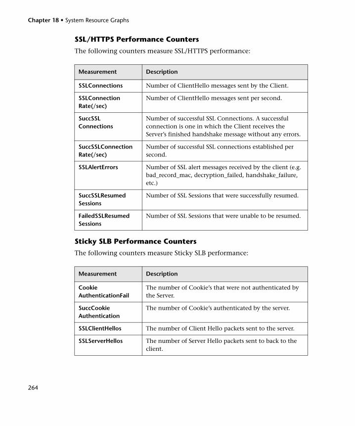
Chapter 18 • System Resource Graphs
264
SSL/HTTPS Performance Counters
The following counters measure SSL/HTTPS performance:
Sticky SLB Performance Counters
The following counters measure Sticky SLB performance:
Measurement Description
SSLConnections Number of ClientHello messages sent by the Client.
SSLConnectionRate(/sec)
Number of ClientHello messages sent per second.
SuccSSLConnections
Number of successful SSL Connections. A successful connection is one in which the Client receives the Server’s finished handshake message without any errors.
SuccSSLConnectionRate(/sec)
Number of successful SSL connections established per second.
SSLAlertErrors Number of SSL alert messages received by the client (e.g. bad_record_mac, decryption_failed, handshake_failure, etc.)
SuccSSLResumedSessions
Number of SSL Sessions that were successfully resumed.
FailedSSLResumedSessions
Number of SSL Sessions that were unable to be resumed.
Measurement Description
CookieAuthenticationFail
The number of Cookie’s that were not authenticated by the Server.
SuccCookieAuthentication
The number of Cookie’s authenticated by the server.
SSLClientHellos The number of Client Hello packets sent to the server.
SSLServerHellos The number of Server Hello packets sent to back to the client.
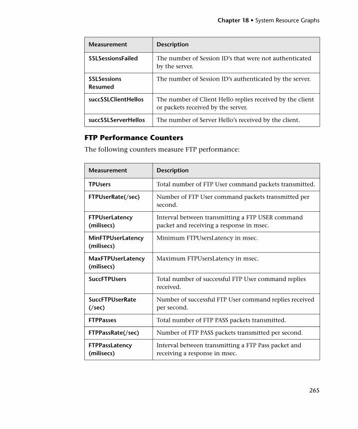
Chapter 18 • System Resource Graphs
265
FTP Performance Counters
The following counters measure FTP performance:
SSLSessionsFailed The number of Session ID’s that were not authenticated by the server.
SSLSessionsResumed
The number of Session ID’s authenticated by the server.
succSSLClientHellos The number of Client Hello replies received by the client or packets received by the server.
succSSLServerHellos The number of Server Hello’s received by the client.
Measurement Description
TPUsers Total number of FTP User command packets transmitted.
FTPUserRate(/sec) Number of FTP User command packets transmitted per second.
FTPUserLatency(milisecs)
Interval between transmitting a FTP USER command packet and receiving a response in msec.
MinFTPUserLatency(milisecs)
Minimum FTPUsersLatency in msec.
MaxFTPUserLatency(milisecs)
Maximum FTPUsersLatency in msec.
SuccFTPUsers Total number of successful FTP User command replies received.
SuccFTPUserRate(/sec)
Number of successful FTP User command replies received per second.
FTPPasses Total number of FTP PASS packets transmitted.
FTPPassRate(/sec) Number of FTP PASS packets transmitted per second.
FTPPassLatency(milisecs)
Interval between transmitting a FTP Pass packet and receiving a response in msec.
Measurement Description
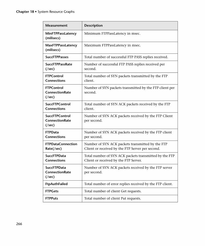
Chapter 18 • System Resource Graphs
266
MinFTPPassLatency(milisecs)
Minimum FTPPassLatency in msec.
MaxFTPPassLatency(milisecs)
Maximum FTPPassLatency in msec.
SuccFTPPasses Total number of successful FTP PASS replies received.
SuccFTPPassRate(/sec)
Number of successful FTP PASS replies received per second.
FTPControlConnections
Total number of SYN packets transmitted by the FTP client.
FTPControlConnectionRate(/sec)
Number of SYN packets transmitted by the FTP client per second.
SuccFTPControlConnections
Total number of SYN ACK packets received by the FTP client.
SuccFTPControlConnectionRate(/sec)
Number of SYN ACK packets received by the FTP Client per second.
FTPDataConnections
Number of SYN ACK packets received by the FTP client per second.
FTPDataConnectionRate(/sec)
Number of SYN ACK packets transmitted by the FTP Client or received by the FTP Server per second.
SuccFTPDataConnections
Total number of SYN ACK packets transmitted by the FTP Client or received by the FTP Server.
SuccFTPDataConnectionRate(/sec)
Number of SYN ACK packets received by the FTP server per second.
FtpAuthFailed Total number of error replies received by the FTP client.
FTPGets Total number of client Get requests.
FTPPuts Total number of client Put requests.
Measurement Description
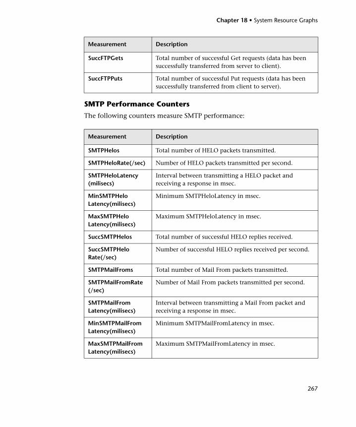
Chapter 18 • System Resource Graphs
267
SMTP Performance Counters
The following counters measure SMTP performance:
SuccFTPGets Total number of successful Get requests (data has been successfully transferred from server to client).
SuccFTPPuts Total number of successful Put requests (data has been successfully transferred from client to server).
Measurement Description
SMTPHelos Total number of HELO packets transmitted.
SMTPHeloRate(/sec) Number of HELO packets transmitted per second.
SMTPHeloLatency(milisecs)
Interval between transmitting a HELO packet and receiving a response in msec.
MinSMTPHeloLatency(milisecs)
Minimum SMTPHeloLatency in msec.
MaxSMTPHeloLatency(milisecs)
Maximum SMTPHeloLatency in msec.
SuccSMTPHelos Total number of successful HELO replies received.
SuccSMTPHeloRate(/sec)
Number of successful HELO replies received per second.
SMTPMailFroms Total number of Mail From packets transmitted.
SMTPMailFromRate(/sec)
Number of Mail From packets transmitted per second.
SMTPMailFromLatency(milisecs)
Interval between transmitting a Mail From packet and receiving a response in msec.
MinSMTPMailFromLatency(milisecs)
Minimum SMTPMailFromLatency in msec.
MaxSMTPMailFromLatency(milisecs)
Maximum SMTPMailFromLatency in msec.
Measurement Description
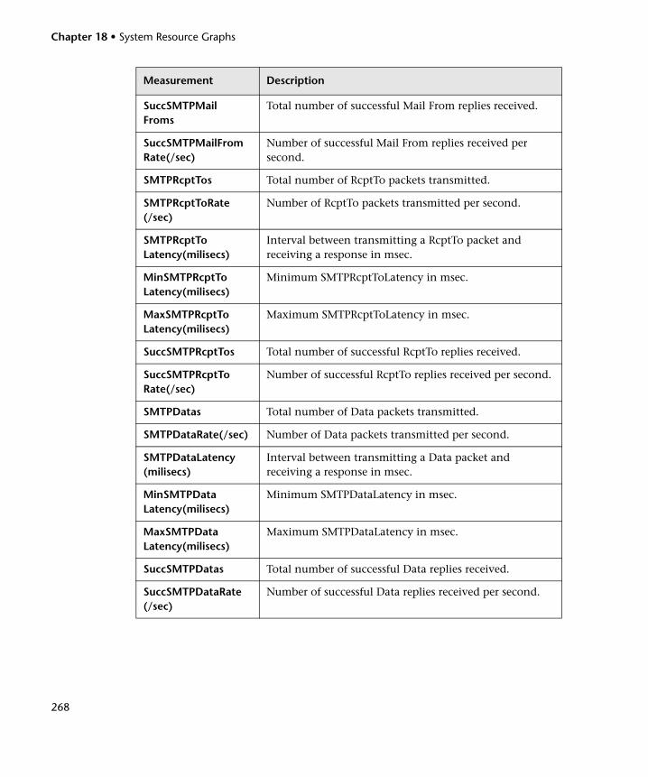
Chapter 18 • System Resource Graphs
268
SuccSMTPMailFroms
Total number of successful Mail From replies received.
SuccSMTPMailFromRate(/sec)
Number of successful Mail From replies received per second.
SMTPRcptTos Total number of RcptTo packets transmitted.
SMTPRcptToRate(/sec)
Number of RcptTo packets transmitted per second.
SMTPRcptToLatency(milisecs)
Interval between transmitting a RcptTo packet and receiving a response in msec.
MinSMTPRcptToLatency(milisecs)
Minimum SMTPRcptToLatency in msec.
MaxSMTPRcptToLatency(milisecs)
Maximum SMTPRcptToLatency in msec.
SuccSMTPRcptTos Total number of successful RcptTo replies received.
SuccSMTPRcptToRate(/sec)
Number of successful RcptTo replies received per second.
SMTPDatas Total number of Data packets transmitted.
SMTPDataRate(/sec) Number of Data packets transmitted per second.
SMTPDataLatency(milisecs)
Interval between transmitting a Data packet and receiving a response in msec.
MinSMTPDataLatency(milisecs)
Minimum SMTPDataLatency in msec.
MaxSMTPDataLatency(milisecs)
Maximum SMTPDataLatency in msec.
SuccSMTPDatas Total number of successful Data replies received.
SuccSMTPDataRate(/sec)
Number of successful Data replies received per second.
Measurement Description
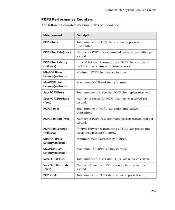
Chapter 18 • System Resource Graphs
269
POP3 Performance Counters
The following counters measure POP3 performance:
Measurement Description
POP3Users Total number of POP3 User command packets transmitted.
POP3UserRate(/sec) Number of POP3 User command packets transmitted per second.
POP3UserLatency(milisecs)
Interval between transmitting a POP3 User command packet and receiving a response in msec.
MinPOP3UserLatency(milisecs)
Minimum POP3UserLatency in msec.
MaxPOP3UserLatency(milisecs)
Maximum POP3UserLatency in msec.
SuccPOP3Users Total number of successful POP3 User replies received.
SuccPOP3UserRate(/sec)
Number of successful POP3 User replies received per second.
POP3Passes Total number of POP3 Pass command packets transmitted.
POP3PassRate(/sec) Number of POP3 Pass command packets transmitted per second.
POP3PassLatency(milisecs)
Interval between transmitting a POP3 Pass packet and receiving a response in msec.
MinPOP3PassLatency(milisecs)
Minimum POP3PassLatency in msec.
MaxPOP3PassLatency(milisecs)
Maximum POP3PassLatency in msec.
SuccPOP3Passes Total number of successful POP3 Pass replies received.
SuccPOP3PassRate(/sec)
Number of successful POP3 Pass replies received per second.
POP3Stats Total number of POP3 Stat command packets sent.
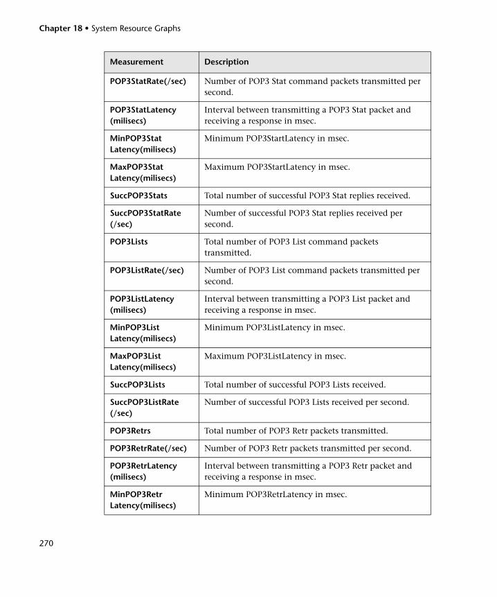
Chapter 18 • System Resource Graphs
270
POP3StatRate(/sec) Number of POP3 Stat command packets transmitted per second.
POP3StatLatency(milisecs)
Interval between transmitting a POP3 Stat packet and receiving a response in msec.
MinPOP3StatLatency(milisecs)
Minimum POP3StartLatency in msec.
MaxPOP3StatLatency(milisecs)
Maximum POP3StartLatency in msec.
SuccPOP3Stats Total number of successful POP3 Stat replies received.
SuccPOP3StatRate(/sec)
Number of successful POP3 Stat replies received per second.
POP3Lists Total number of POP3 List command packets transmitted.
POP3ListRate(/sec) Number of POP3 List command packets transmitted per second.
POP3ListLatency(milisecs)
Interval between transmitting a POP3 List packet and receiving a response in msec.
MinPOP3ListLatency(milisecs)
Minimum POP3ListLatency in msec.
MaxPOP3ListLatency(milisecs)
Maximum POP3ListLatency in msec.
SuccPOP3Lists Total number of successful POP3 Lists received.
SuccPOP3ListRate(/sec)
Number of successful POP3 Lists received per second.
POP3Retrs Total number of POP3 Retr packets transmitted.
POP3RetrRate(/sec) Number of POP3 Retr packets transmitted per second.
POP3RetrLatency(milisecs)
Interval between transmitting a POP3 Retr packet and receiving a response in msec.
MinPOP3RetrLatency(milisecs)
Minimum POP3RetrLatency in msec.
Measurement Description
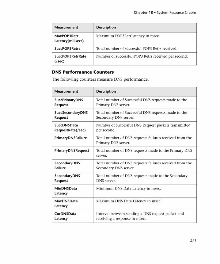
Chapter 18 • System Resource Graphs
271
DNS Performance Counters
The following counters measure DNS performance:
MaxPOP3RetrLatency(milisecs)
Maximum POP3RetrLatency in msec.
SuccPOP3Retrs Total number of successful POP3 Retrs received.
SuccPOP3RetrRate(/sec)
Number of successful POP3 Retrs received per second.
Measurement Description
SuccPrimaryDNSRequest
Total number of Successful DNS requests made to the Primary DNS server.
SuccSecondaryDNSRequest
Total number of Successful DNS requests made to the Secondary DNS server.
SuccDNSDataRequestRate(/sec)
Number of Successful DNS Request packets transmitted per second.
PrimaryDNSFailure Total number of DNS requests failures received from the Primary DNS server.
PrimaryDNSRequest Total number of DNS requests made to the Primary DNS server.
SecondaryDNSFailure
Total number of DNS requests failures received from the Secondary DNS server.
SecondaryDNSRequest
Total number of DNS requests made to the Secondary DNS server.
MinDNSDataLatency
Minimum DNS Data Latency in msec.
MaxDNSDataLatency
Maximum DNS Data Latency in msec.
CurDNSDataLatency
Interval between sending a DNS request packet and receiving a response in msec.
Measurement Description
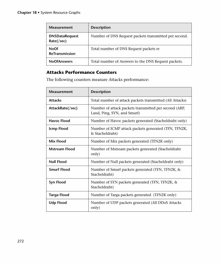
Chapter 18 • System Resource Graphs
272
Attacks Performance Counters
The following counters measure Attacks performance:
DNSDataRequestRate(/sec)
Number of DNS Request packets transmitted per second.
NoOfReTransmission
Total number of DNS Request packets re
NoOfAnswers Total number of Answers to the DNS Request packets.
Measurement Description
Attacks Total number of attack packets transmitted (All Attacks)
AttackRate(/sec) Number of attack packets transmitted per second (ARP, Land, Ping, SYN, and Smurf)
Havoc Flood Number of Havoc packets generated (Stacheldraht only)
Icmp Flood Number of ICMP attack packets generated (TFN, TFN2K, & Stacheldraht)
Mix Flood Number of Mix packets generated (TFN2K only)
Mstream Flood Number of Mstream packets generated (Stacheldraht only)
Null Flood Number of Null packets generated (Stacheldraht only)
Smurf Flood Number of Smurf packets generated (TFN, TFN2K, & Stacheldraht)
Syn Flood Number of SYN packets generated (TFN, TFN2K, & Stacheldraht)
Targa Flood Number of Targa packets generated (TFN2K only)
Udp Flood Number of UDP packets generated (All DDoS Attacks only)
Measurement Description
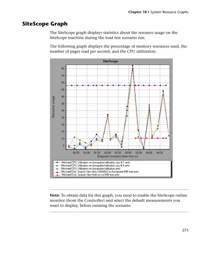
Chapter 18 • System Resource Graphs
273
SiteScope Graph
The SiteScope graph displays statistics about the resource usage on the SiteScope machine during the load test scenario run.
The following graph displays the percentage of memory resources used, the number of pages read per second, and the CPU utilization:
Note: To obtain data for this graph, you need to enable the SiteScope online monitor (from the Controller) and select the default measurements you want to display, before running the scenario.

Chapter 18 • System Resource Graphs
274
275
19 Network Monitor Graphs
You can use Network graphs to determine whether your network is causing a delay in the load test scenario. You can also determine the problematic network segment.
This chapter includes:
➤ About Network Monitoring on page 275
➤ Understanding Network Monitoring on page 276
➤ Network Delay Time Graph on page 277
➤ Network Sub-Path Time Graph on page 278
➤ Network Segment Delay Graph on page 279
➤ Verifying the Network as a Bottleneck on page 280
About Network Monitoring
Network configuration is a primary factor in the performance of applications and Web systems. A poorly designed network can slow client activity to unacceptable levels.
In an application, there are many network segments. A single network segment with poor performance can affect the entire application.
Network graphs let you locate the network-related problem so that it can be fixed.
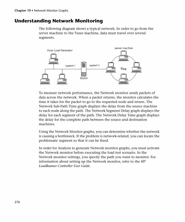
Chapter 19 • Network Monitor Graphs
276
Understanding Network Monitoring
The following diagram shows a typical network. In order to go from the server machine to the Vuser machine, data must travel over several segments.
To measure network performance, the Network monitor sends packets of data across the network. When a packet returns, the monitor calculates the time it takes for the packet to go to the requested node and return. The Network Sub-Path Time graph displays the delay from the source machine to each node along the path. The Network Segment Delay graph displays the delay for each segment of the path. The Network Delay Time graph displays the delay for the complete path between the source and destination machines.
Using the Network Monitor graphs, you can determine whether the network is causing a bottleneck. If the problem is network-related, you can locate the problematic segment so that it can be fixed.
In order for Analysis to generate Network monitor graphs, you must activate the Network monitor before executing the load test scenario. In the Network monitor settings, you specify the path you want to monitor. For information about setting up the Network monitor, refer to the HP LoadRunner Controller User Guide.
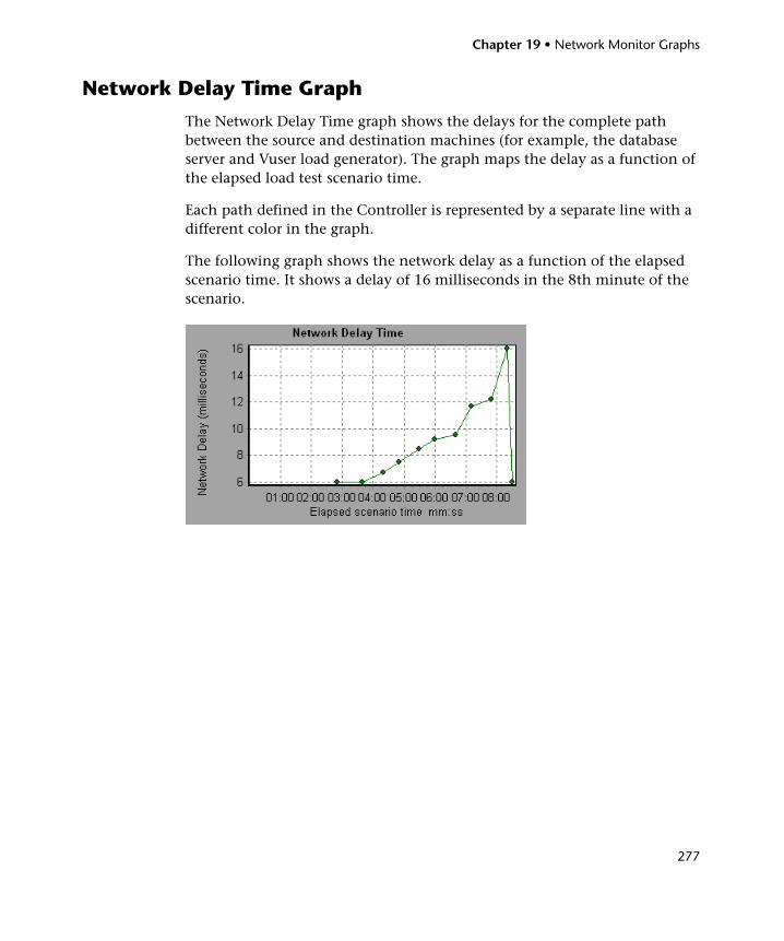
Chapter 19 • Network Monitor Graphs
277
Network Delay Time Graph
The Network Delay Time graph shows the delays for the complete path between the source and destination machines (for example, the database server and Vuser load generator). The graph maps the delay as a function of the elapsed load test scenario time.
Each path defined in the Controller is represented by a separate line with a different color in the graph.
The following graph shows the network delay as a function of the elapsed scenario time. It shows a delay of 16 milliseconds in the 8th minute of the scenario.
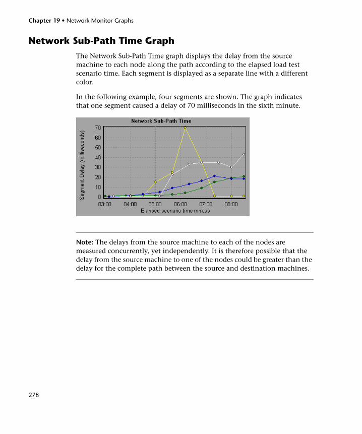
Chapter 19 • Network Monitor Graphs
278
Network Sub-Path Time Graph
The Network Sub-Path Time graph displays the delay from the source machine to each node along the path according to the elapsed load test scenario time. Each segment is displayed as a separate line with a different color.
In the following example, four segments are shown. The graph indicates that one segment caused a delay of 70 milliseconds in the sixth minute.
Note: The delays from the source machine to each of the nodes are measured concurrently, yet independently. It is therefore possible that the delay from the source machine to one of the nodes could be greater than the delay for the complete path between the source and destination machines.
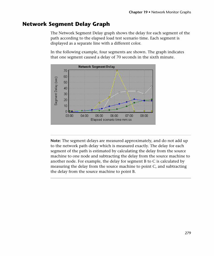
Chapter 19 • Network Monitor Graphs
279
Network Segment Delay Graph
The Network Segment Delay graph shows the delay for each segment of the path according to the elapsed load test scenario time. Each segment is displayed as a separate line with a different color.
In the following example, four segments are shown. The graph indicates that one segment caused a delay of 70 seconds in the sixth minute.
Note: The segment delays are measured approximately, and do not add up to the network path delay which is measured exactly. The delay for each segment of the path is estimated by calculating the delay from the source machine to one node and subtracting the delay from the source machine to another node. For example, the delay for segment B to C is calculated by measuring the delay from the source machine to point C, and subtracting the delay from the source machine to point B.
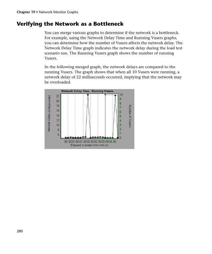
Chapter 19 • Network Monitor Graphs
280
Verifying the Network as a Bottleneck
You can merge various graphs to determine if the network is a bottleneck. For example, using the Network Delay Time and Running Vusers graphs, you can determine how the number of Vusers affects the network delay. The Network Delay Time graph indicates the network delay during the load test scenario run. The Running Vusers graph shows the number of running Vusers.
In the following merged graph, the network delays are compared to the running Vusers. The graph shows that when all 10 Vusers were running, a network delay of 22 milliseconds occurred, implying that the network may be overloaded.
281
20 Firewall Server Monitor Graphs
After a load test scenario run, you can use the Firewall server monitor graphs to analyze Firewall server performance.
This chapter includes:
➤ About Firewall Server Monitor Graphs on page 281
➤ Check Point FireWall-1 Server Graph on page 282
About Firewall Server Monitor Graphs
Firewall server monitor graphs provide you with performance information for firewall servers. In order to obtain data for this graph, you need to activate the Firewall server online monitor before running the load test scenario. When you set up the online monitor for the Firewall server, you indicate which statistics and measurements to monitor. For more information on activating and configuring Firewall server monitors, refer to the HP LoadRunner Controller User Guide.
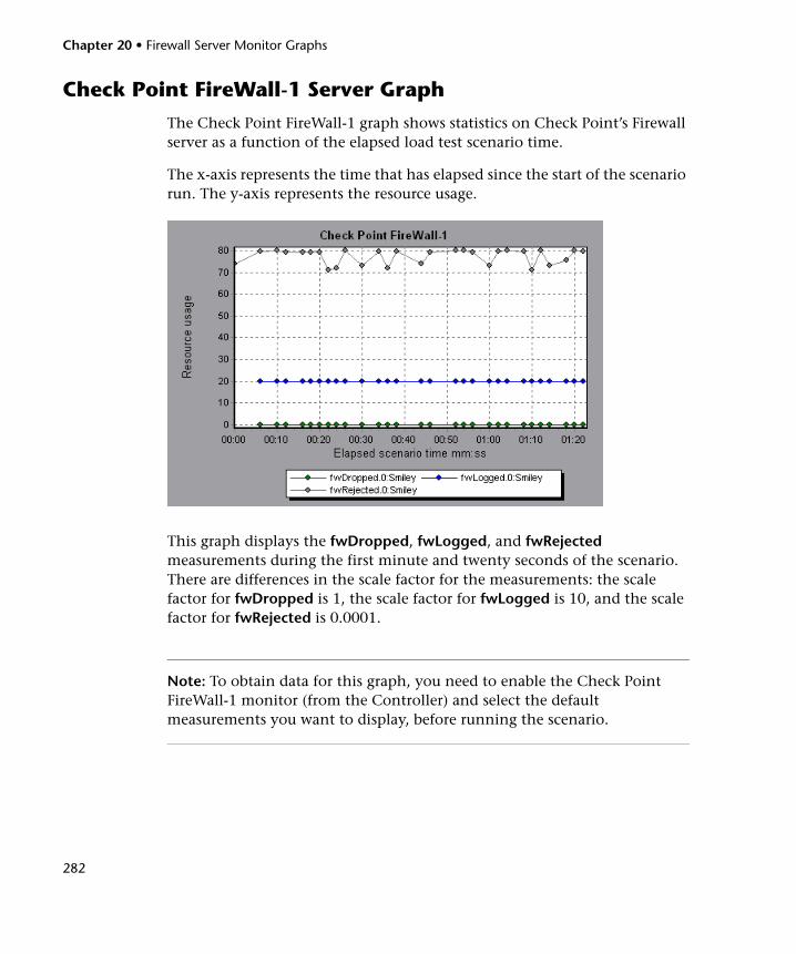
Chapter 20 • Firewall Server Monitor Graphs
282
Check Point FireWall-1 Server Graph
The Check Point FireWall-1 graph shows statistics on Check Point’s Firewall server as a function of the elapsed load test scenario time.
The x-axis represents the time that has elapsed since the start of the scenario run. The y-axis represents the resource usage.
This graph displays the fwDropped, fwLogged, and fwRejected measurements during the first minute and twenty seconds of the scenario. There are differences in the scale factor for the measurements: the scale factor for fwDropped is 1, the scale factor for fwLogged is 10, and the scale factor for fwRejected is 0.0001.
Note: To obtain data for this graph, you need to enable the Check Point FireWall-1 monitor (from the Controller) and select the default measurements you want to display, before running the scenario.
Chapter 20 • Firewall Server Monitor Graphs
283
The following measurements are available for the Check Point FireWall-1 server:
Measurement Description
fwRejected The number of rejected packets.
fwDropped The number of dropped packets.
fwLogged The number of logged packets.

Chapter 20 • Firewall Server Monitor Graphs
284
285
21 Web Server Resource Graphs
After a load test scenario run, you can use Web Server Resource graphs to analyze the performance of your Apache, Microsoft IIS, iPlanet/Netscape, and iPlanet (SNMP) server performance.
This chapter includes:
➤ About Web Server Resource Graphs on page 286
➤ Apache Server Graph on page 287
➤ Microsoft Information Internet Server (IIS) Graph on page 289
➤ iPlanet/Netscape Server Graph on page 291
➤ iPlanet (SNMP) Server Graph on page 293

Chapter 21 • Web Server Resource Graphs
286
About Web Server Resource Graphs
Web Server Resource graphs provide you with information about the resource usage of the Apache, Microsoft IIS, iPlanet/Netscape, and iPlanet (SNMP) Web servers. In order to obtain data for these graphs, you need to activate the online monitor for the server and specify which resources you want to measure before running the load test scenario. For information on activating and configuring the Web Server Resource monitors, refer to the HP LoadRunner Controller User Guide.
In order to display all the measurements on a single graph, Analysis may scale them. The Legend window indicates the scale factor for each resource. To obtain the true value, multiply the scale factor by the displayed value. For example, in the following graph the actual value of KBytes Sent per second in the second minute is 1; 10 multiplied by the scale factor of 1/10 (indicated in the Legend window below).
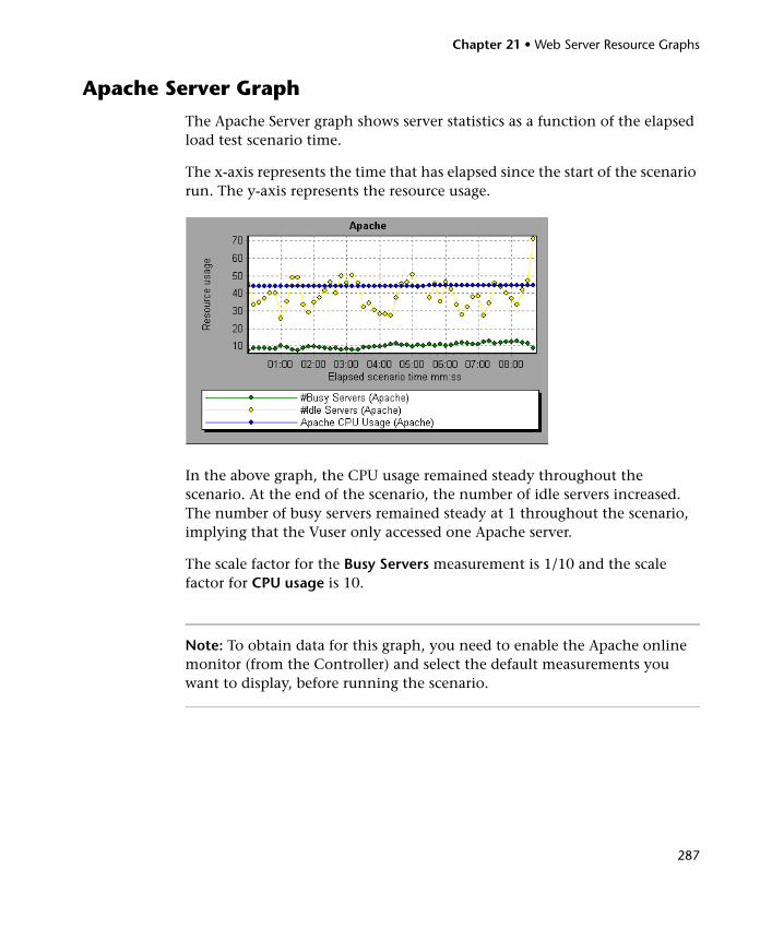
Chapter 21 • Web Server Resource Graphs
287
Apache Server Graph
The Apache Server graph shows server statistics as a function of the elapsed load test scenario time.
The x-axis represents the time that has elapsed since the start of the scenario run. The y-axis represents the resource usage.
In the above graph, the CPU usage remained steady throughout the scenario. At the end of the scenario, the number of idle servers increased. The number of busy servers remained steady at 1 throughout the scenario, implying that the Vuser only accessed one Apache server.
The scale factor for the Busy Servers measurement is 1/10 and the scale factor for CPU usage is 10.
Note: To obtain data for this graph, you need to enable the Apache online monitor (from the Controller) and select the default measurements you want to display, before running the scenario.
Chapter 21 • Web Server Resource Graphs
288
The following default measurements are available for the Apache server:
Note: The Apache monitor connects to the Web server in order to gather statistics, and registers one hit for each sampling. The Apache graph, therefore, always displays one hit per second, even if no clients are connected to the Apache server.
Measurement Description
# Busy Servers The number of servers in the Busy state
# Idle Servers The number of servers in the Idle state
Apache CPU Usage The percentage of time the CPU is utilized by the Apache server
Hits/sec The HTTP request rate
KBytes Sent/sec The rate at which data bytes are sent from the Web server
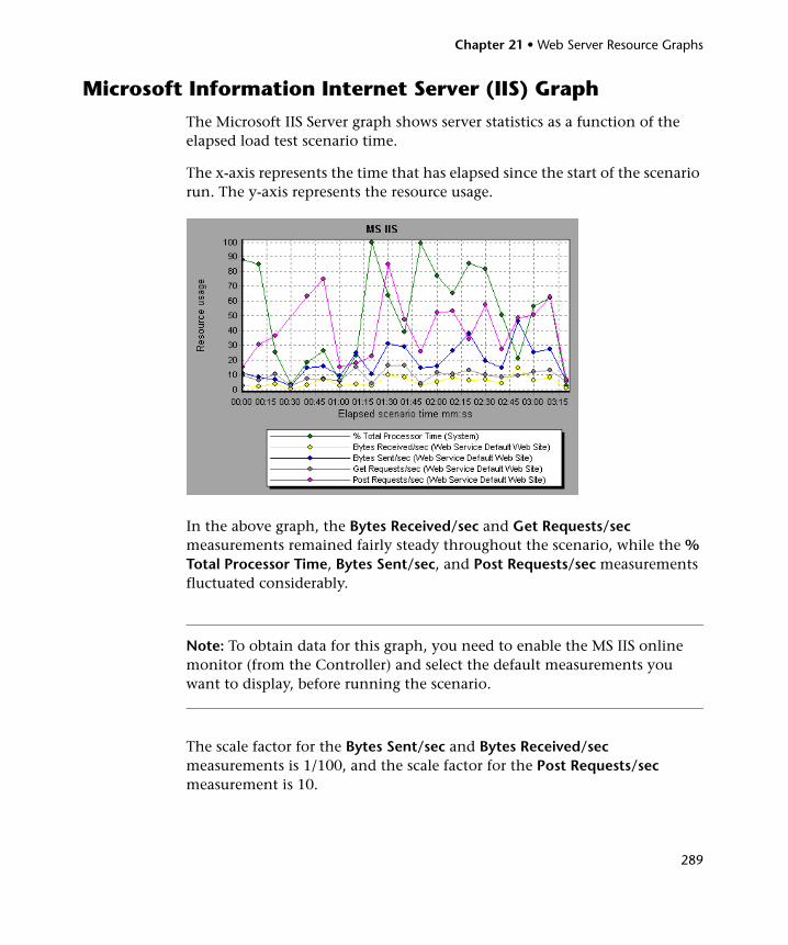
Chapter 21 • Web Server Resource Graphs
289
Microsoft Information Internet Server (IIS) Graph
The Microsoft IIS Server graph shows server statistics as a function of the elapsed load test scenario time.
The x-axis represents the time that has elapsed since the start of the scenario run. The y-axis represents the resource usage.
In the above graph, the Bytes Received/sec and Get Requests/sec measurements remained fairly steady throughout the scenario, while the % Total Processor Time, Bytes Sent/sec, and Post Requests/sec measurements fluctuated considerably.
Note: To obtain data for this graph, you need to enable the MS IIS online monitor (from the Controller) and select the default measurements you want to display, before running the scenario.
The scale factor for the Bytes Sent/sec and Bytes Received/sec measurements is 1/100, and the scale factor for the Post Requests/sec measurement is 10.
Chapter 21 • Web Server Resource Graphs
290
The following default measurements are available for the IIS server:
Object Measurement Description
Web Service
Bytes Sent/sec The rate at which the data bytes are sent by the Web service.
Web Service
Bytes Received/sec
The rate at which the data bytes are received by the Web service.
Web Service
Get Requests/sec The rate at which HTTP requests using the GET method are made. Get requests are generally used for basic file retrievals or image maps, though they can be used with forms.
Web Service
Post Requests/sec The rate at which HTTP requests using the POST method are made. Post requests are generally used for forms or gateway requests.
Web Service
Maximum Connections
The maximum number of simultaneous connections established with the Web service.
Web Service
Current Connections
The current number of connections established with the Web service.
Web Service
Current NonAnonymous Users
The number of users that currently have a non-anonymous connection using the Web service.
Web Service
Not Found Errors/sec
The rate of errors due to requests that could not be satisfied by the server because the requested document could not be found. These are generally reported to the client as an HTTP 404 error code.
Process Private Bytes The current number of bytes that the process has allocated that cannot be shared with other processes.
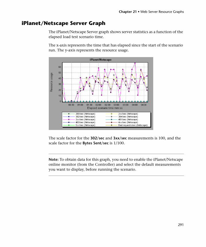
Chapter 21 • Web Server Resource Graphs
291
iPlanet/Netscape Server Graph
The iPlanet/Netscape Server graph shows server statistics as a function of the elapsed load test scenario time.
The x-axis represents the time that has elapsed since the start of the scenario run. The y-axis represents the resource usage.
The scale factor for the 302/sec and 3xx/sec measurements is 100, and the scale factor for the Bytes Sent/sec is 1/100.
Note: To obtain data for this graph, you need to enable the iPlanet/Netscape online monitor (from the Controller) and select the default measurements you want to display, before running the scenario.
Chapter 21 • Web Server Resource Graphs
292
The following default measurements are available for the iPlanet/Netscape server:
Measurement Description
200/sec The rate of successful transactions being processed by the server
2xx/sec The rate at which the server handles status codes in the 200 to 299 range
302/sec The rate of relocated URLs being processed by the server
304/sec The rate of requests for which the server tells the user to use a local copy of a URL instead of retrieving a newer version from the server
3xx/sec The rate at which the server handles status codes in the 300 to 399 range
401/sec The rate of unauthorized requests handled by the server
403/sec The rate of forbidden URL status codes handled by the server
4xx/sec The rate at which the server handles status codes in the 400 to 499 range
5xx/sec The rate at which the server handles status codes 500 and higher
Bad requests/sec The rate at which the server handles bad requests
Bytes sent/sec The rate at which bytes of data are sent from the Web server
Hits/sec The HTTP request rate
xxx/sec The rate of all status codes (2xx-5xx) handled by the server, excluding timeouts and other errors that did return an HTTP status code
Chapter 21 • Web Server Resource Graphs
293
iPlanet (SNMP) Server Graph
The iPlanet (SNMP) Server graph shows server statistics as a function of the elapsed load test scenario time.
The x-axis represents the time that has elapsed since the start of the scenario run. The y-axis represents the resource usage.
Note: To obtain data for this graph, you need to enable the iPlanet (SNMP) online monitor (from the Controller) and select the default measurements you want to display, before running the scenario.
The following default measurements are available for the iPlanet (SNMP) server:
Measurement Description
iwsInstanceTable iPlanet Web Server instances
iwsInstanceEntry iPlanet Web Server instances
iwsInstanceIndex Server instance index
iwsInstanceId Server instance identifier
iwsInstanceVersion Server instance software version
iwsInstanceDescription Description of server instance
iwsInstanceOrganization Organization responsible for server instance
iwsInstanceContact Contact information for person(s) responsible for server instance
iwsInstanceLocation Location of server instance
iwsInstanceStatus Server instance status
iwsInstanceUptime Server instance uptime
iwsInstanceDeathCount Number of times server instance processes have died
Chapter 21 • Web Server Resource Graphs
294
iwsInstanceRequests Number of requests processed
iwsInstanceInOctets Number of octets received
iwsInstanceOutOctets Number of octets transmitted
iwsInstanceCount2xx Number of 200-level (Successful) responses issued
iwsInstanceCount3xx Number of 300-level (Redirection) responses issued
iwsInstanceCount4xx Number of 400-level (Client Error) responses issued
iwsInstanceCount5xx Number of 500-level (Server Error) responses issued
iwsInstanceCountOther Number of other (neither 2xx, 3xx, 4xx, nor 5xx) responses issued
iwsInstanceCount200 Number of 200 (OK) responses issued
iwsInstanceCount302 Number of 302 (Moved Temporarily) responses issued
iwsInstanceCount304 Number of 304 (Not Modified) responses issued
iwsInstanceCount400 Number of 400 (Bad Request) responses issued
iwsInstanceCount401 Number of 401 (Unauthorized) responses issued
iwsInstanceCount403 Number of 403 (Forbidden) responses issued
iwsInstanceCount404 Number of 404 (Not Found) responses issued
iwsInstanceCount503 Number of 503 (Unavailable) responses issued
iwsInstanceLoad1MinuteAverage
System load average for 1 minute
iwsInstanceLoad5MinuteAverage
System load average for 5 minutes
iwsInstanceLoad15MinuteAverage
System load average for 15 minutes
Measurement Description
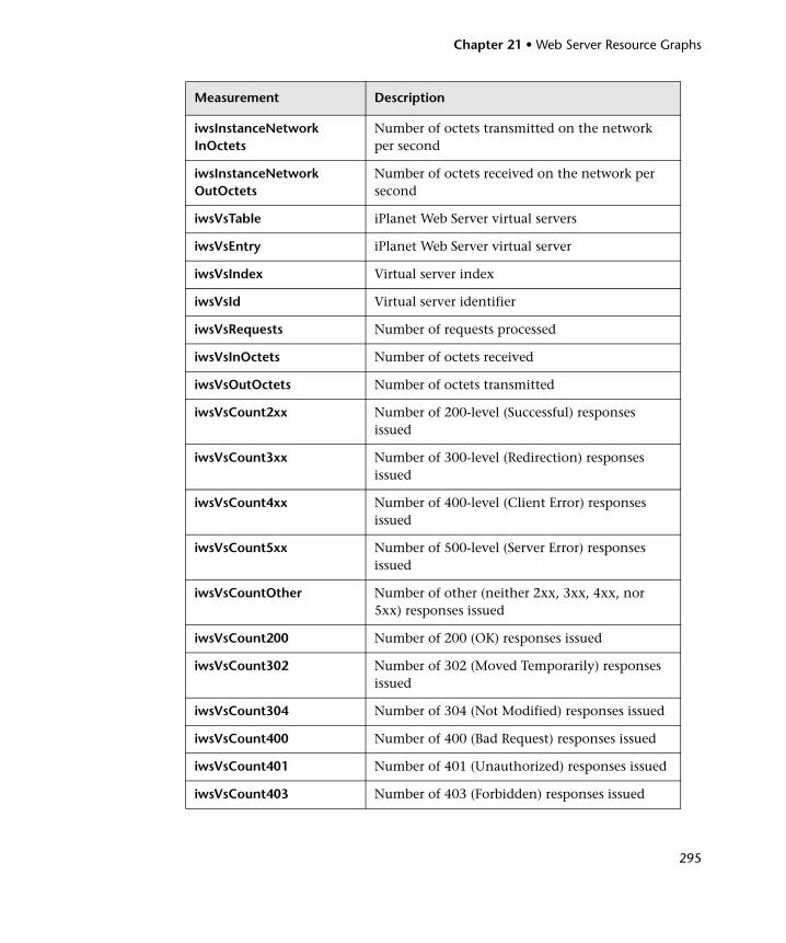
Chapter 21 • Web Server Resource Graphs
295
iwsInstanceNetworkInOctets
Number of octets transmitted on the network per second
iwsInstanceNetworkOutOctets
Number of octets received on the network per second
iwsVsTable iPlanet Web Server virtual servers
iwsVsEntry iPlanet Web Server virtual server
iwsVsIndex Virtual server index
iwsVsId Virtual server identifier
iwsVsRequests Number of requests processed
iwsVsInOctets Number of octets received
iwsVsOutOctets Number of octets transmitted
iwsVsCount2xx Number of 200-level (Successful) responses issued
iwsVsCount3xx Number of 300-level (Redirection) responses issued
iwsVsCount4xx Number of 400-level (Client Error) responses issued
iwsVsCount5xx Number of 500-level (Server Error) responses issued
iwsVsCountOther Number of other (neither 2xx, 3xx, 4xx, nor 5xx) responses issued
iwsVsCount200 Number of 200 (OK) responses issued
iwsVsCount302 Number of 302 (Moved Temporarily) responses issued
iwsVsCount304 Number of 304 (Not Modified) responses issued
iwsVsCount400 Number of 400 (Bad Request) responses issued
iwsVsCount401 Number of 401 (Unauthorized) responses issued
iwsVsCount403 Number of 403 (Forbidden) responses issued
Measurement Description
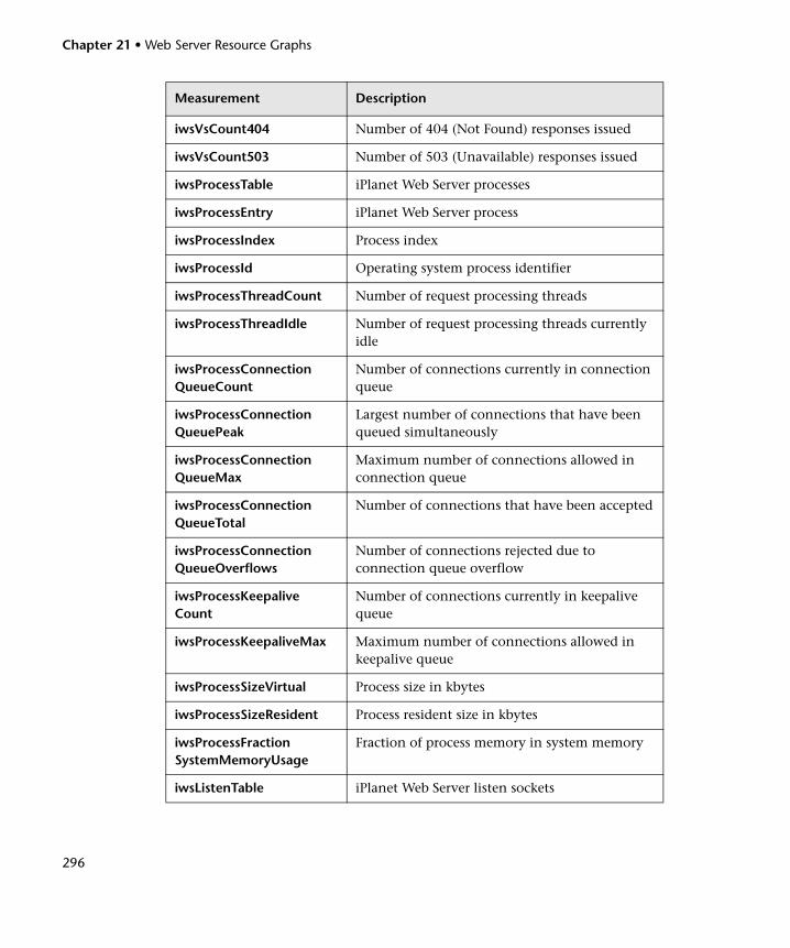
Chapter 21 • Web Server Resource Graphs
296
iwsVsCount404 Number of 404 (Not Found) responses issued
iwsVsCount503 Number of 503 (Unavailable) responses issued
iwsProcessTable iPlanet Web Server processes
iwsProcessEntry iPlanet Web Server process
iwsProcessIndex Process index
iwsProcessId Operating system process identifier
iwsProcessThreadCount Number of request processing threads
iwsProcessThreadIdle Number of request processing threads currently idle
iwsProcessConnectionQueueCount
Number of connections currently in connection queue
iwsProcessConnectionQueuePeak
Largest number of connections that have been queued simultaneously
iwsProcessConnectionQueueMax
Maximum number of connections allowed in connection queue
iwsProcessConnectionQueueTotal
Number of connections that have been accepted
iwsProcessConnectionQueueOverflows
Number of connections rejected due to connection queue overflow
iwsProcessKeepaliveCount
Number of connections currently in keepalive queue
iwsProcessKeepaliveMax Maximum number of connections allowed in keepalive queue
iwsProcessSizeVirtual Process size in kbytes
iwsProcessSizeResident Process resident size in kbytes
iwsProcessFractionSystemMemoryUsage
Fraction of process memory in system memory
iwsListenTable iPlanet Web Server listen sockets
Measurement Description
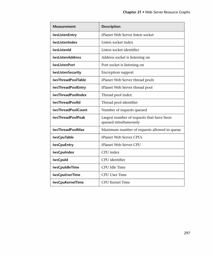
Chapter 21 • Web Server Resource Graphs
297
iwsListenEntry iPlanet Web Server listen socket
iwsListenIndex Listen socket index
iwsListenId Listen socket identifier
iwsListenAddress Address socket is listening on
iwsListenPort Port socket is listening on
iwsListenSecurity Encryption support
iwsThreadPoolTable iPlanet Web Server thread pools
iwsThreadPoolEntry iPlanet Web Server thread pool
iwsThreadPoolIndex Thread pool index
iwsThreadPoolId Thread pool identifier
iwsThreadPoolCount Number of requests queued
iwsThreadPoolPeak Largest number of requests that have been queued simultaneously
iwsThreadPoolMax Maximum number of requests allowed in queue
iwsCpuTable iPlanet Web Server CPUs
iwsCpuEntry iPlanet Web Server CPU
iwsCpuIndex CPU index
iwsCpuId CPU identifier
iwsCpuIdleTime CPU Idle Time
iwsCpuUserTime CPU User Time
iwsCpuKernelTime CPU Kernel Time
Measurement Description

Chapter 21 • Web Server Resource Graphs
298
299
22 Web Application Server Resource Graphs
After a load test scenario run, you can use Web Application Server Resource graphs to analyze Web application server performance.
This chapter includes:
➤ About Web Application Server Resource Graphs on page 300
➤ Ariba Graph on page 301
➤ ATG Dynamo Graph on page 304
➤ BroadVision Graph on page 308
➤ ColdFusion Graph on page 316
➤ Fujitsu INTERSTAGE Graph on page 318
➤ iPlanet (NAS) Graph on page 319
➤ Microsoft Active Server Pages (ASP) Graph on page 328
➤ Oracle9iAS HTTP Server Graph on page 329
➤ SilverStream Graph on page 334
➤ WebLogic (SNMP) Graph on page 336
➤ WebLogic (JMX) Graph on page 339
➤ WebSphere Graph on page 342
➤ WebSphere Application Server Graph on page 349
➤ WebSphere (EPM) Graph on page 353
Chapter 22 • Web Application Server Resource Graphs
300
About Web Application Server Resource Graphs
Web Application Server Resource graphs provide you with resource usage information about the Ariba, ATG Dynamo, BroadVision, ColdFusion, Fujitsu INTERSTAGE, iPlanet (NAS), Microsoft ASP, Oracle9iAS HTTP, SilverStream, WebLogic (SNMP), WebLogic (JMX), and WebSphere application servers.
In order to obtain data for these graphs, you need to activate the online monitor for the application server and specify which resources you want to measure before running the load test scenario. For information on activating and configuring the Web Application Server Resource monitors, refer to the HP LoadRunner Controller User Guide.
When you open a Web Application Server Resource graph, you can filter it to show only the relevant application. When you need to analyze other applications, you can change the filter conditions and display the desired resources.
In order to display all the measurements on a single graph, Analysis may scale them. The Legend window indicates the scale factor for each resource. To obtain the true value, multiply the scale factor by the displayed value. For more information on scaled measurements, see the example in “About Web Server Resource Graphs” on page 286.
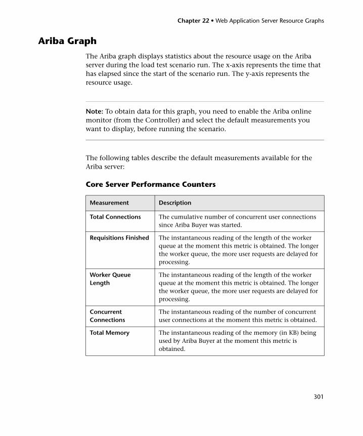
Chapter 22 • Web Application Server Resource Graphs
301
Ariba Graph
The Ariba graph displays statistics about the resource usage on the Ariba server during the load test scenario run. The x-axis represents the time that has elapsed since the start of the scenario run. The y-axis represents the resource usage.
Note: To obtain data for this graph, you need to enable the Ariba online monitor (from the Controller) and select the default measurements you want to display, before running the scenario.
The following tables describe the default measurements available for the Ariba server:
Core Server Performance Counters
Measurement Description
Total Connections The cumulative number of concurrent user connections since Ariba Buyer was started.
Requisitions Finished The instantaneous reading of the length of the worker queue at the moment this metric is obtained. The longer the worker queue, the more user requests are delayed for processing.
Worker Queue Length
The instantaneous reading of the length of the worker queue at the moment this metric is obtained. The longer the worker queue, the more user requests are delayed for processing.
Concurrent Connections
The instantaneous reading of the number of concurrent user connections at the moment this metric is obtained.
Total Memory The instantaneous reading of the memory (in KB) being used by Ariba Buyer at the moment this metric is obtained.
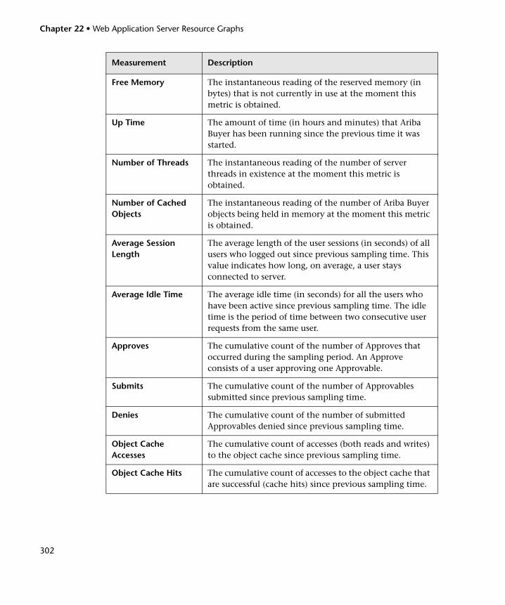
Chapter 22 • Web Application Server Resource Graphs
302
Free Memory The instantaneous reading of the reserved memory (in bytes) that is not currently in use at the moment this metric is obtained.
Up Time The amount of time (in hours and minutes) that Ariba Buyer has been running since the previous time it was started.
Number of Threads The instantaneous reading of the number of server threads in existence at the moment this metric is obtained.
Number of Cached Objects
The instantaneous reading of the number of Ariba Buyer objects being held in memory at the moment this metric is obtained.
Average Session Length
The average length of the user sessions (in seconds) of all users who logged out since previous sampling time. This value indicates how long, on average, a user stays connected to server.
Average Idle Time The average idle time (in seconds) for all the users who have been active since previous sampling time. The idle time is the period of time between two consecutive user requests from the same user.
Approves The cumulative count of the number of Approves that occurred during the sampling period. An Approve consists of a user approving one Approvable.
Submits The cumulative count of the number of Approvables submitted since previous sampling time.
Denies The cumulative count of the number of submitted Approvables denied since previous sampling time.
Object Cache Accesses
The cumulative count of accesses (both reads and writes) to the object cache since previous sampling time.
Object Cache Hits The cumulative count of accesses to the object cache that are successful (cache hits) since previous sampling time.
Measurement Description
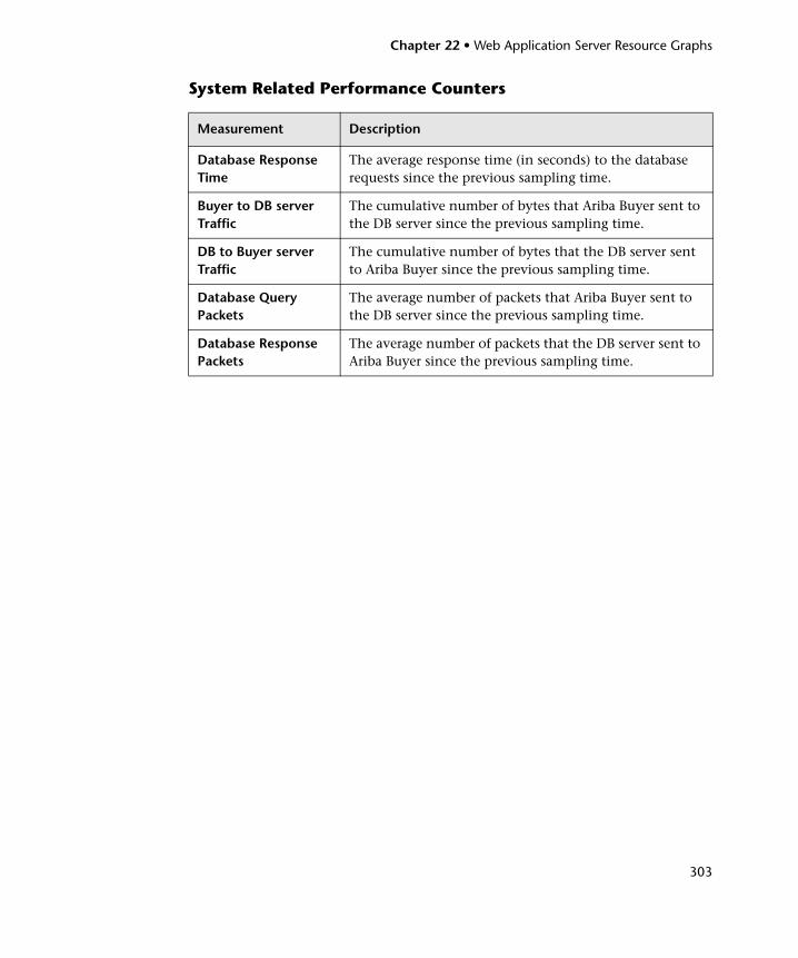
Chapter 22 • Web Application Server Resource Graphs
303
System Related Performance Counters
Measurement Description
Database Response Time
The average response time (in seconds) to the database requests since the previous sampling time.
Buyer to DB server Traffic
The cumulative number of bytes that Ariba Buyer sent to the DB server since the previous sampling time.
DB to Buyer server Traffic
The cumulative number of bytes that the DB server sent to Ariba Buyer since the previous sampling time.
Database Query Packets
The average number of packets that Ariba Buyer sent to the DB server since the previous sampling time.
Database Response Packets
The average number of packets that the DB server sent to Ariba Buyer since the previous sampling time.
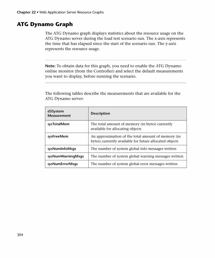
Chapter 22 • Web Application Server Resource Graphs
304
ATG Dynamo Graph
The ATG Dynamo graph displays statistics about the resource usage on the ATG Dynamo server during the load test scenario run. The x-axis represents the time that has elapsed since the start of the scenario run. The y-axis represents the resource usage.
Note: To obtain data for this graph, you need to enable the ATG Dynamo online monitor (from the Controller) and select the default measurements you want to display, before running the scenario.
The following tables describe the measurements that are available for the ATG Dynamo server:
d3System Measurement
Description
sysTotalMem The total amount of memory (in bytes) currently available for allocating objects
sysFreeMem An approximation of the total amount of memory (in bytes) currently available for future allocated objects
sysNumInfoMsgs The number of system global info messages written
sysNumWarningMsgs The number of system global warning messages written
sysNumErrorMsgs The number of system global error messages written
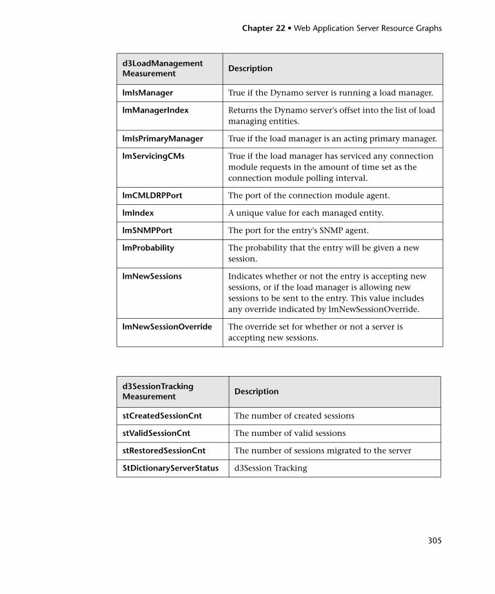
Chapter 22 • Web Application Server Resource Graphs
305
d3LoadManagement Measurement
Description
lmIsManager True if the Dynamo server is running a load manager.
lmManagerIndex Returns the Dynamo server's offset into the list of load managing entities.
lmIsPrimaryManager True if the load manager is an acting primary manager.
lmServicingCMs True if the load manager has serviced any connection module requests in the amount of time set as the connection module polling interval.
lmCMLDRPPort The port of the connection module agent.
lmIndex A unique value for each managed entity.
lmSNMPPort The port for the entry's SNMP agent.
lmProbability The probability that the entry will be given a new session.
lmNewSessions Indicates whether or not the entry is accepting new sessions, or if the load manager is allowing new sessions to be sent to the entry. This value includes any override indicated by lmNewSessionOverride.
lmNewSessionOverride The override set for whether or not a server is accepting new sessions.
d3SessionTracking Measurement
Description
stCreatedSessionCnt The number of created sessions
stValidSessionCnt The number of valid sessions
stRestoredSessionCnt The number of sessions migrated to the server
StDictionaryServerStatus d3Session Tracking
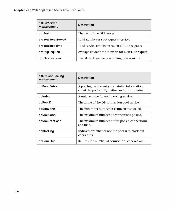
Chapter 22 • Web Application Server Resource Graphs
306
d3DRPServer Measurement
Description
drpPort The port of the DRP server
drpTotalReqsServed Total number of DRP requests serviced
drpTotalReqTime Total service time in msecs for all DRP requests
drpAvgReqTime Average service time in msecs for each DRP request
drpNewSessions True if the Dynamo is accepting new sessions
d3DBConnPooling Measurement
Description
dbPoolsEntry A pooling service entry containing information about the pool configuration and current status.
dbIndex A unique value for each pooling service.
dbPoolID The name of the DB connection pool service.
dbMinConn The minimum number of connections pooled.
dbMaxConn The maximum number of connections pooled.
dbMaxFreeConn The maximum number of free pooled connections at a time.
dbBlocking Indicates whether or not the pool is to block out check outs.
dbConnOut Returns the number of connections checked out.
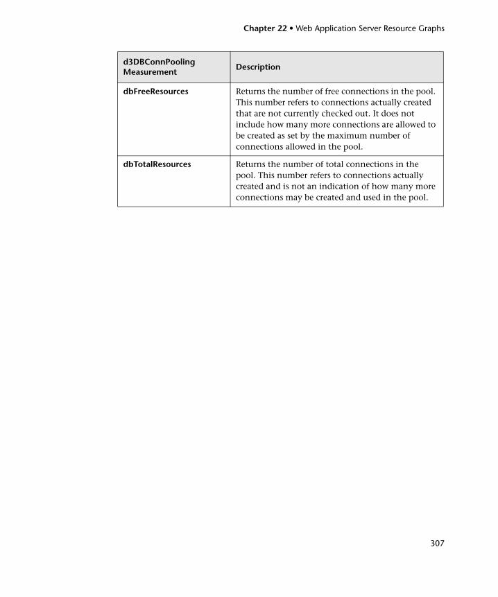
Chapter 22 • Web Application Server Resource Graphs
307
dbFreeResources Returns the number of free connections in the pool. This number refers to connections actually created that are not currently checked out. It does not include how many more connections are allowed to be created as set by the maximum number of connections allowed in the pool.
dbTotalResources Returns the number of total connections in the pool. This number refers to connections actually created and is not an indication of how many more connections may be created and used in the pool.
d3DBConnPooling Measurement
Description
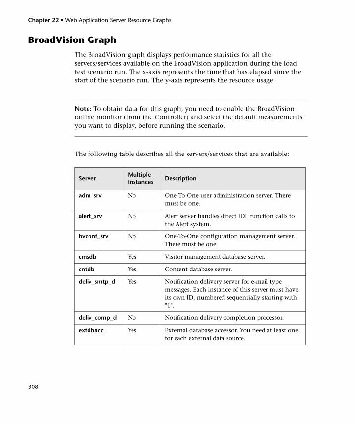
Chapter 22 • Web Application Server Resource Graphs
308
BroadVision Graph
The BroadVision graph displays performance statistics for all the servers/services available on the BroadVision application during the load test scenario run. The x-axis represents the time that has elapsed since the start of the scenario run. The y-axis represents the resource usage.
Note: To obtain data for this graph, you need to enable the BroadVision online monitor (from the Controller) and select the default measurements you want to display, before running the scenario.
The following table describes all the servers/services that are available:
ServerMultiple Instances
Description
adm_srv No One-To-One user administration server. There must be one.
alert_srv No Alert server handles direct IDL function calls to the Alert system.
bvconf_srv No One-To-One configuration management server. There must be one.
cmsdb Yes Visitor management database server.
cntdb Yes Content database server.
deliv_smtp_d Yes Notification delivery server for e-mail type messages. Each instance of this server must have its own ID, numbered sequentially starting with "1".
deliv_comp_d No Notification delivery completion processor.
extdbacc Yes External database accessor. You need at least one for each external data source.
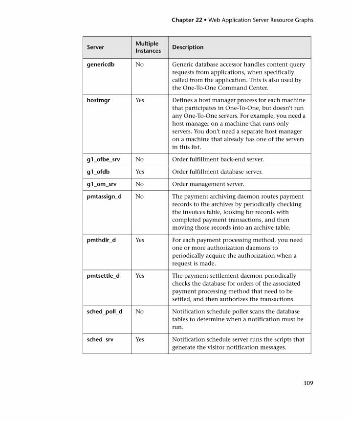
Chapter 22 • Web Application Server Resource Graphs
309
genericdb No Generic database accessor handles content query requests from applications, when specifically called from the application. This is also used by the One-To-One Command Center.
hostmgr Yes Defines a host manager process for each machine that participates in One-To-One, but doesn't run any One-To-One servers. For example, you need a host manager on a machine that runs only servers. You don't need a separate host manager on a machine that already has one of the servers in this list.
g1_ofbe_srv No Order fulfillment back-end server.
g1_ofdb Yes Order fulfillment database server.
g1_om_srv No Order management server.
pmtassign_d No The payment archiving daemon routes payment records to the archives by periodically checking the invoices table, looking for records with completed payment transactions, and then moving those records into an archive table.
pmthdlr_d Yes For each payment processing method, you need one or more authorization daemons to periodically acquire the authorization when a request is made.
pmtsettle_d Yes The payment settlement daemon periodically checks the database for orders of the associated payment processing method that need to be settled, and then authorizes the transactions.
sched_poll_d No Notification schedule poller scans the database tables to determine when a notification must be run.
sched_srv Yes Notification schedule server runs the scripts that generate the visitor notification messages.
ServerMultiple Instances
Description
Chapter 22 • Web Application Server Resource Graphs
310
Performance Counters
Performance counters for each server/service are divided into logical groups according to the service type.
The following section describes all the available counters under each group.
Note: For some services the number of counters for the same group can be different.
Counter groups:
➤ BV_DB_STAT
➤ BV_SRV_CTRL
➤ BV_SRV_STAT
➤ NS_STAT
➤ BV_CACHE_STAT
➤ JS_SCRIPT_CTRL
➤ JS_SCRIPT_STAT
BV_DB_STAT
The database accessor processes have additional statistics available from the BV_DB_STAT memory block. These statistics provide information about database accesses, including the count of selects, updates, inserts, deletes, and stored procedure executions.
➤ DELETE. Count of delete executions
➤ INSERT. Count of insert executions
➤ SELECT. Count of select executions
➤ SPROC. Count of stored procedure executions.
➤ UPDATE. Count of update executions
Chapter 22 • Web Application Server Resource Graphs
311
BV_SRV_CTRL
➤ SHUTDOWN
BV_SRV_STAT
The display for Interaction Manager processes includes information about the current count of sessions, connections, idle sessions, threads in use, and count of CGI requests processed.
➤ HOST. Host machine running the process.
➤ ID. Instance of the process (of which multiple can be configured in the bv1to1.conf file), or engine ID of the Interaction Manager.
➤ CGI. Current count of CGI requests processed.
➤ CONN. Current count of connections.
➤ CPU. CPU percentage consumed by this process. If a process is using most of the CPU time, consider moving it to another host, or creating an additional process, possibly running on another machine. Both of these specifications are done in the bv1to1.conf file. The CPU % reported is against a single processor. If a server is taking up a whole CPU on a 4 processor machine, this statistic will report 100%, while the Windows NT Task Manager will report 25%. The value reported by this statistic is consistent with "% Processor Time" on the Windows NT Performance Monitor.
➤ GROUP. Process group (which is defined in the bv1to1.conf file), or Interaction Manager application name.
➤ STIME. Start time of server. The start times should be relatively close. Later times might be an indication that a server crashed and was automatically restarted.
➤ IDL. Total count of IDL requests received, not including those to the monitor.
➤ IdlQ
➤ JOB
➤ LWP. Number of light-weight processes (threads).
➤ RSS. Resident memory size of server process (in kilobytes).
Chapter 22 • Web Application Server Resource Graphs
312
➤ STIME. System start time.
➤ SESS. Current count of sessions.
➤ SYS. Accumulated system mode CPU time (seconds).
➤ THR. Current count of threads.
➤ USR. Accumulated user mode CPU time (seconds).
➤ VSZ. Virtual memory size of server process (in kilobytes). If a process is growing in size, it probably has a memory leak. If it is an Interaction Manager process, the culprit is most likely a component or dynamic object (though Interaction Manager servers do grow and shrink from garbage collection during normal use).
NS_STAT
The NS process displays the namespace for the current One-To-One environment, and optionally can update objects in a name space.
➤ Bind
➤ List
➤ New
➤ Rebnd
➤ Rsolv
➤ Unbnd
Chapter 22 • Web Application Server Resource Graphs
313
BV_CACHE_STAT
Monitors the request cache status.
The available counters for each request are:
➤ CNT- Request_Name-HIT. Count of requests found in the cache.
➤ CNT- Request_Name-MAX. Maximum size of the cache in bytes.
➤ CNT- Request_Name-SWAP. Count of items that got swapped out of the cache.
➤ CNT- Request_Name-MISS. Count of requests that were not in the cache.
➤ CNT- Request_Name-SIZE. Count of items currently in the cache.
Chapter 22 • Web Application Server Resource Graphs
314
Cache Metrics
Cache metrics are available for the following items:
➤ AD
➤ ALERTSCHED. Notification schedules are defined in the BV_ALERTSCHED and BV_MSGSCHED tables. They are defined by the One-To-One Command Center user or by an application.
➤ CATEGORY_CONTENT
➤ DISCUSSION. The One-To-One discussion groups provide moderated systems of messages and threads of messages aligned to a particular topic. Use the Discussion group interfaces for creating, retrieving and deleting individual messages in a discussion group. To create, delete, or retrieve discussion groups, use the generic content management API. The BV_DiscussionDB object provides access to the threads and messages in the discussion group database.
➤ EXT_FIN_PRODUCT
➤ EDITORIAL. Using the Editorials content module, you can point cast and community cast personalized editorial content, and sell published text on your One-To-One site. You can solicit editorial content, such as investment reports and weekly columns, from outside authors and publishers, and create your own articles, reviews, reports, and other informative media. In addition to text, you can use images, sounds, music, and video presentations as editorial content.
➤ INCENTIVE. Contains sales incentives.
➤ MSGSCHED. Contains the specifications of visitor-message jobs. Notification schedules are defined in the BV_ALERTSCHED and BV_MSGSCHED tables. They are defined by the One-To-One Command Center user or by an application.
➤ MSGSCRIPT. Contains the descriptions of the JavaScripts that generate visitor messages and alert messages. Contains the descriptions of the JavaScripts that generate targeted messages and alert messages. Use the Command Center to add message script information to this table by selecting the Visitor Messages module in the Notifications group. For more information, refer to the Command Center User's Guide.
Chapter 22 • Web Application Server Resource Graphs
315
➤ PRODUCT. BV_PRODUCT contains information about the products that a visitor can purchase.
➤ QUERY. BV_QUERY contains queries.
➤ SCRIPT. BV_SCRIPT contains page scripts.
➤ SECURITIES
➤ TEMPLATE. The Templates content module enables you to store in the content database any BroadVision page templates used on your One-To-One site. Combining BroadVision page templates with BroadVision dynamic objects in the One-To-One Design Center application is one way for site developers to create One-To-One Web sites. If your developers use these page templates, you can use the Command Center to enter and manage them in your content database. If your site doesn't use BroadVision page template, you will not use this content module.
JS_SCRIPT_CTRL
➤ CACHE
➤ DUMP
➤ FLUSH
➤ METER
➤ TRACE
JS_SCRIPT_STAT
➤ ALLOC
➤ ERROR
➤ FAIL
➤ JSPPERR
➤ RELEASE
➤ STOP
➤ SUCC
➤ SYNTAX
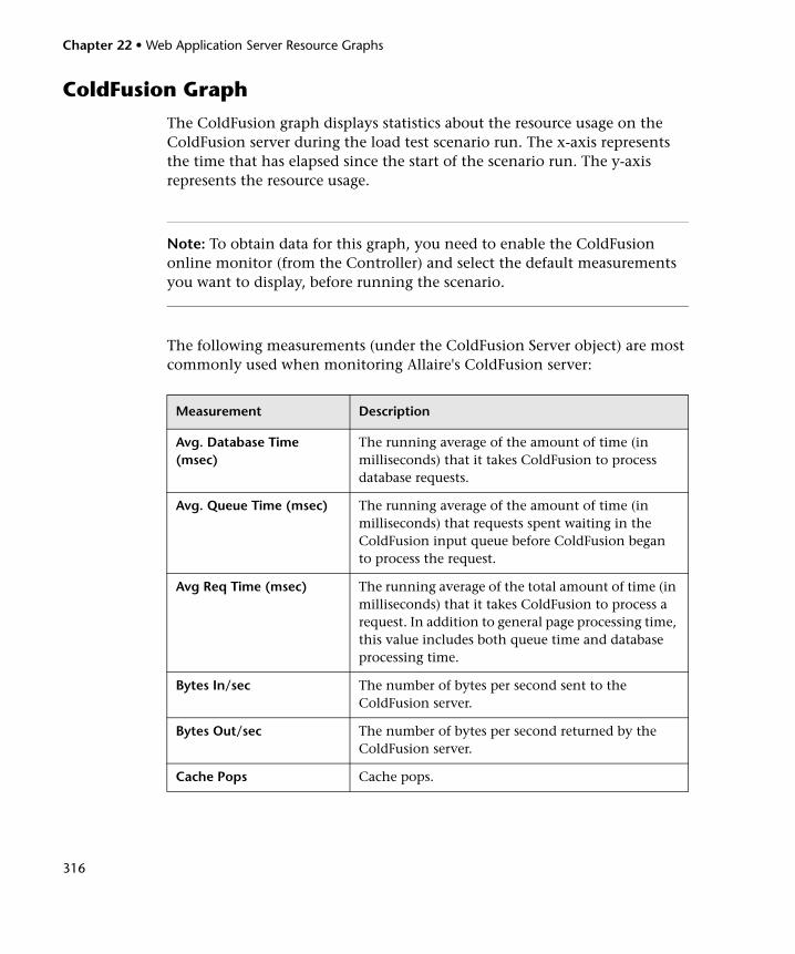
Chapter 22 • Web Application Server Resource Graphs
316
ColdFusion Graph
The ColdFusion graph displays statistics about the resource usage on the ColdFusion server during the load test scenario run. The x-axis represents the time that has elapsed since the start of the scenario run. The y-axis represents the resource usage.
Note: To obtain data for this graph, you need to enable the ColdFusion online monitor (from the Controller) and select the default measurements you want to display, before running the scenario.
The following measurements (under the ColdFusion Server object) are most commonly used when monitoring Allaire's ColdFusion server:
Measurement Description
Avg. Database Time (msec)
The running average of the amount of time (in milliseconds) that it takes ColdFusion to process database requests.
Avg. Queue Time (msec) The running average of the amount of time (in milliseconds) that requests spent waiting in the ColdFusion input queue before ColdFusion began to process the request.
Avg Req Time (msec) The running average of the total amount of time (in milliseconds) that it takes ColdFusion to process a request. In addition to general page processing time, this value includes both queue time and database processing time.
Bytes In/sec The number of bytes per second sent to the ColdFusion server.
Bytes Out/sec The number of bytes per second returned by the ColdFusion server.
Cache Pops Cache pops.
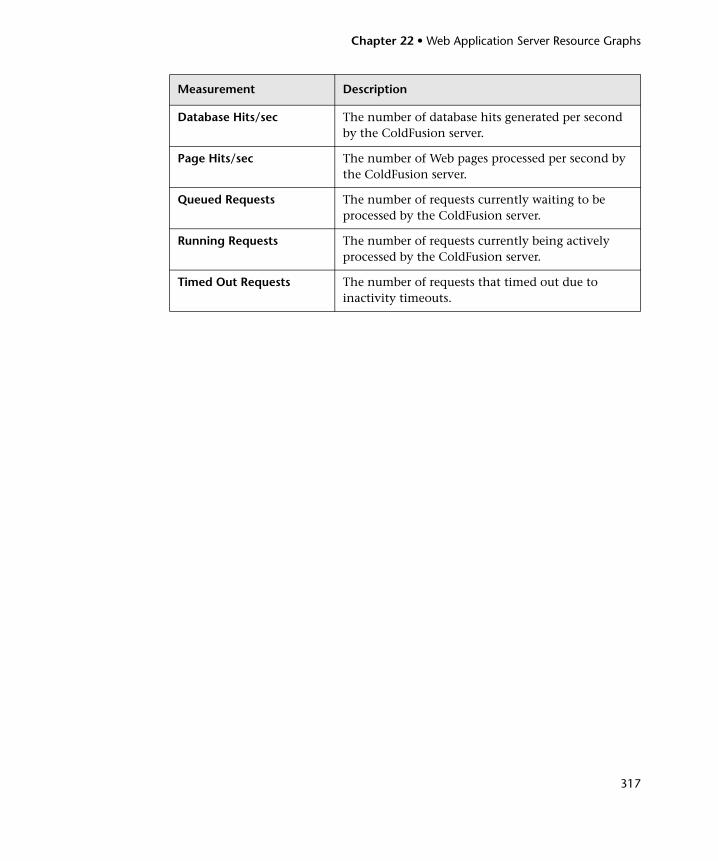
Chapter 22 • Web Application Server Resource Graphs
317
Database Hits/sec The number of database hits generated per second by the ColdFusion server.
Page Hits/sec The number of Web pages processed per second by the ColdFusion server.
Queued Requests The number of requests currently waiting to be processed by the ColdFusion server.
Running Requests The number of requests currently being actively processed by the ColdFusion server.
Timed Out Requests The number of requests that timed out due to inactivity timeouts.
Measurement Description
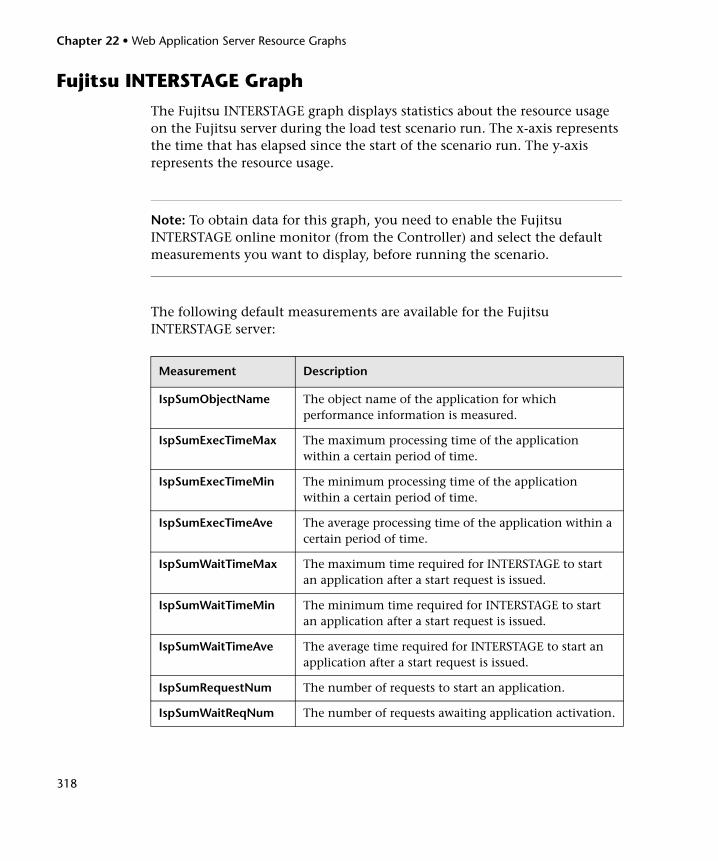
Chapter 22 • Web Application Server Resource Graphs
318
Fujitsu INTERSTAGE Graph
The Fujitsu INTERSTAGE graph displays statistics about the resource usage on the Fujitsu server during the load test scenario run. The x-axis represents the time that has elapsed since the start of the scenario run. The y-axis represents the resource usage.
Note: To obtain data for this graph, you need to enable the Fujitsu INTERSTAGE online monitor (from the Controller) and select the default measurements you want to display, before running the scenario.
The following default measurements are available for the Fujitsu INTERSTAGE server:
Measurement Description
IspSumObjectName The object name of the application for which performance information is measured.
IspSumExecTimeMax The maximum processing time of the application within a certain period of time.
IspSumExecTimeMin The minimum processing time of the application within a certain period of time.
IspSumExecTimeAve The average processing time of the application within a certain period of time.
IspSumWaitTimeMax The maximum time required for INTERSTAGE to start an application after a start request is issued.
IspSumWaitTimeMin The minimum time required for INTERSTAGE to start an application after a start request is issued.
IspSumWaitTimeAve The average time required for INTERSTAGE to start an application after a start request is issued.
IspSumRequestNum The number of requests to start an application.
IspSumWaitReqNum The number of requests awaiting application activation.
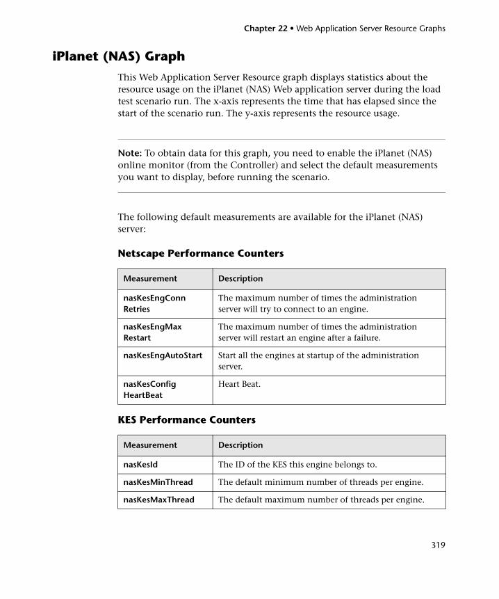
Chapter 22 • Web Application Server Resource Graphs
319
iPlanet (NAS) Graph
This Web Application Server Resource graph displays statistics about the resource usage on the iPlanet (NAS) Web application server during the load test scenario run. The x-axis represents the time that has elapsed since the start of the scenario run. The y-axis represents the resource usage.
Note: To obtain data for this graph, you need to enable the iPlanet (NAS) online monitor (from the Controller) and select the default measurements you want to display, before running the scenario.
The following default measurements are available for the iPlanet (NAS) server:
Netscape Performance Counters
KES Performance Counters
Measurement Description
nasKesEngConnRetries
The maximum number of times the administration server will try to connect to an engine.
nasKesEngMaxRestart
The maximum number of times the administration server will restart an engine after a failure.
nasKesEngAutoStart Start all the engines at startup of the administration server.
nasKesConfigHeartBeat
Heart Beat.
Measurement Description
nasKesId The ID of the KES this engine belongs to.
nasKesMinThread The default minimum number of threads per engine.
nasKesMaxThread The default maximum number of threads per engine.
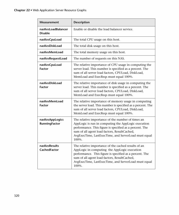
Chapter 22 • Web Application Server Resource Graphs
320
nasKesLoadBalancerDisable
Enable or disable the load balancer service.
nasKesCpuLoad The total CPU usage on this host.
nasKesDiskLoad The total disk usage on this host.
nasKesMemLoad The total memory usage on this host.
nasKesRequestLoad The number of requests on this NAS.
nasKesCpuLoadFactor
The relative importance of CPU usage in computing the server load. This number is specified as a percent. The sum of all server load factors, CPULoad, DiskLoad, MemLoad and ExecReqs must equal 100%.
nasKesDiskLoadFactor
The relative importance of disk usage in computing the server load. This number is specified as a percent. The sum of all server load factors, CPULoad, DiskLoad, MemLoad and ExecReqs must equal 100%.
nasKesMemLoadFactor
The relative importance of memory usage in computing the server load. This number is specified as a percent. The sum of all server load factors, CPULoad, DiskLoad, MemLoad and ExecReqs must equal 100%.
nasKesAppLogicsRunningFactor
The relative importance of the number of times an AppLogic is run in computing the AppLogic execution performance. This figure is specified as a percent. The sum of all agent load factors, ResultCached, AvgExecTime, LastExecTime, and ServerLoad must equal 100%.
nasKesResultsCachedFactor
The relative importance of the cached results of an AppLogic in computing the AppLogic execution performance. This figure is specified as a percent. The sum of all agent load factors, ResultCached, AvgExecTime, LastExecTime, and ServerLoad must equal 100%.
Measurement Description
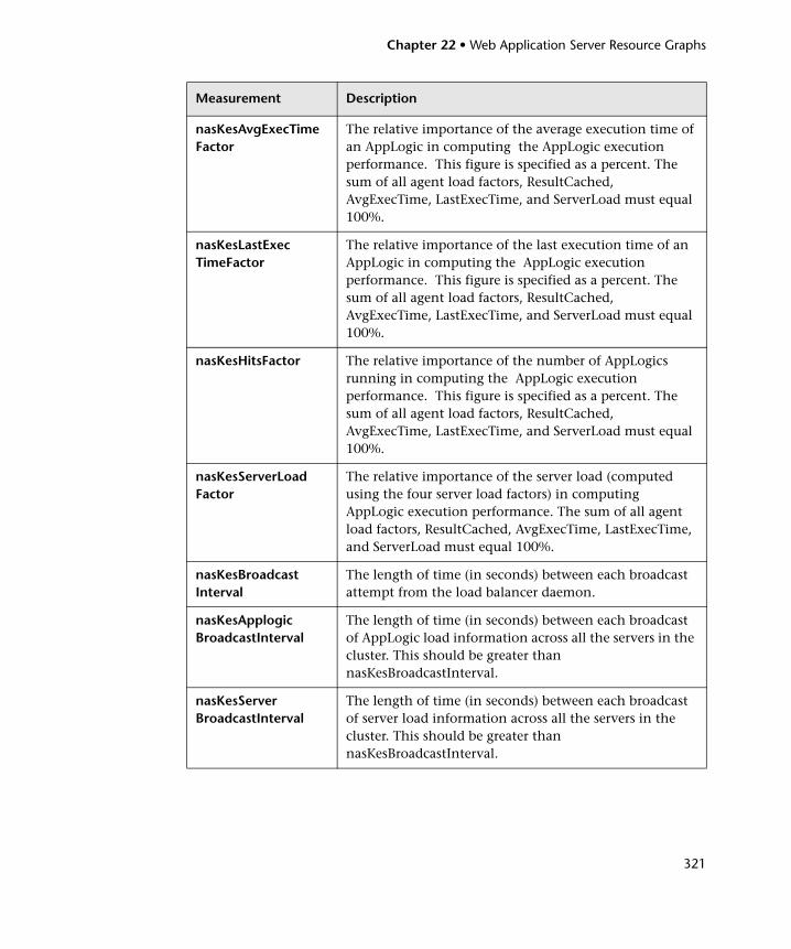
Chapter 22 • Web Application Server Resource Graphs
321
nasKesAvgExecTimeFactor
The relative importance of the average execution time of an AppLogic in computing the AppLogic execution performance. This figure is specified as a percent. The sum of all agent load factors, ResultCached, AvgExecTime, LastExecTime, and ServerLoad must equal 100%.
nasKesLastExecTimeFactor
The relative importance of the last execution time of an AppLogic in computing the AppLogic execution performance. This figure is specified as a percent. The sum of all agent load factors, ResultCached, AvgExecTime, LastExecTime, and ServerLoad must equal 100%.
nasKesHitsFactor The relative importance of the number of AppLogics running in computing the AppLogic execution performance. This figure is specified as a percent. The sum of all agent load factors, ResultCached, AvgExecTime, LastExecTime, and ServerLoad must equal 100%.
nasKesServerLoadFactor
The relative importance of the server load (computed using the four server load factors) in computing AppLogic execution performance. The sum of all agent load factors, ResultCached, AvgExecTime, LastExecTime, and ServerLoad must equal 100%.
nasKesBroadcastInterval
The length of time (in seconds) between each broadcast attempt from the load balancer daemon.
nasKesApplogicBroadcastInterval
The length of time (in seconds) between each broadcast of AppLogic load information across all the servers in the cluster. This should be greater than nasKesBroadcastInterval.
nasKesServerBroadcastInterval
The length of time (in seconds) between each broadcast of server load information across all the servers in the cluster. This should be greater than nasKesBroadcastInterval.
Measurement Description
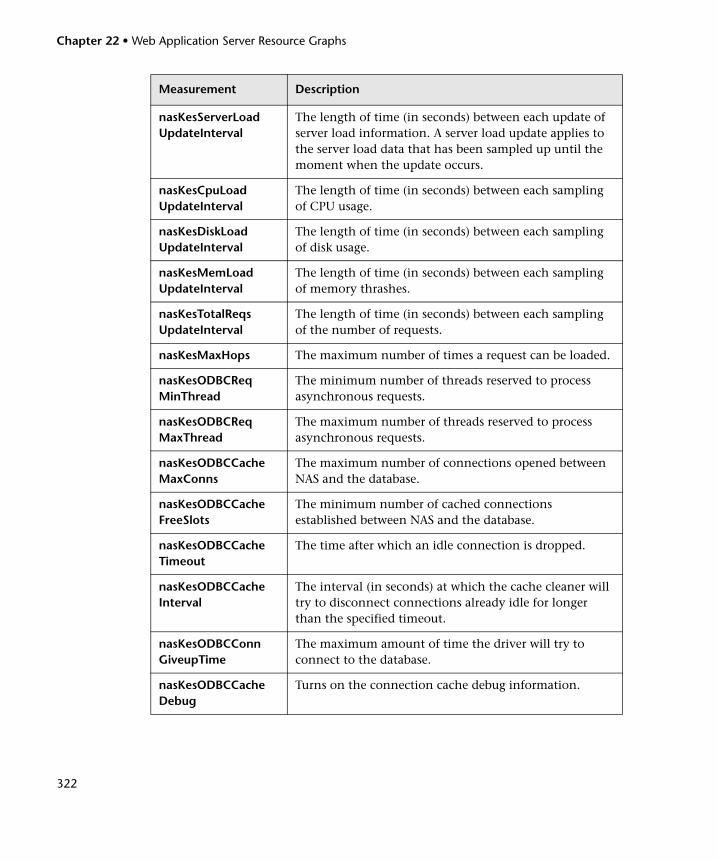
Chapter 22 • Web Application Server Resource Graphs
322
nasKesServerLoadUpdateInterval
The length of time (in seconds) between each update of server load information. A server load update applies to the server load data that has been sampled up until the moment when the update occurs.
nasKesCpuLoadUpdateInterval
The length of time (in seconds) between each sampling of CPU usage.
nasKesDiskLoadUpdateInterval
The length of time (in seconds) between each sampling of disk usage.
nasKesMemLoadUpdateInterval
The length of time (in seconds) between each sampling of memory thrashes.
nasKesTotalReqsUpdateInterval
The length of time (in seconds) between each sampling of the number of requests.
nasKesMaxHops The maximum number of times a request can be loaded.
nasKesODBCReqMinThread
The minimum number of threads reserved to process asynchronous requests.
nasKesODBCReqMaxThread
The maximum number of threads reserved to process asynchronous requests.
nasKesODBCCacheMaxConns
The maximum number of connections opened between NAS and the database.
nasKesODBCCacheFreeSlots
The minimum number of cached connections established between NAS and the database.
nasKesODBCCacheTimeout
The time after which an idle connection is dropped.
nasKesODBCCacheInterval
The interval (in seconds) at which the cache cleaner will try to disconnect connections already idle for longer than the specified timeout.
nasKesODBCConnGiveupTime
The maximum amount of time the driver will try to connect to the database.
nasKesODBCCacheDebug
Turns on the connection cache debug information.
Measurement Description
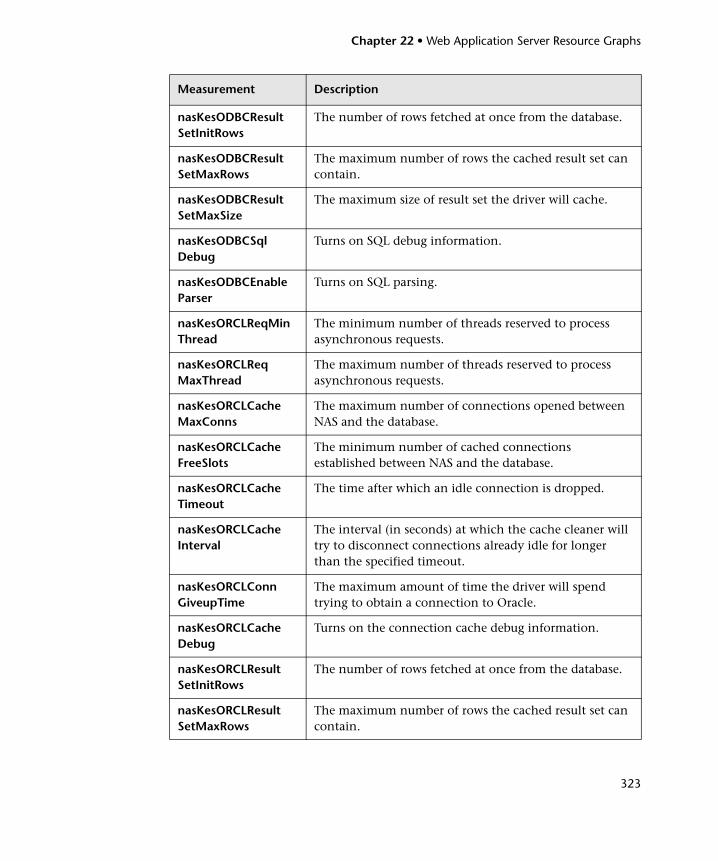
Chapter 22 • Web Application Server Resource Graphs
323
nasKesODBCResultSetInitRows
The number of rows fetched at once from the database.
nasKesODBCResultSetMaxRows
The maximum number of rows the cached result set can contain.
nasKesODBCResultSetMaxSize
The maximum size of result set the driver will cache.
nasKesODBCSqlDebug
Turns on SQL debug information.
nasKesODBCEnableParser
Turns on SQL parsing.
nasKesORCLReqMinThread
The minimum number of threads reserved to process asynchronous requests.
nasKesORCLReqMaxThread
The maximum number of threads reserved to process asynchronous requests.
nasKesORCLCacheMaxConns
The maximum number of connections opened between NAS and the database.
nasKesORCLCacheFreeSlots
The minimum number of cached connections established between NAS and the database.
nasKesORCLCacheTimeout
The time after which an idle connection is dropped.
nasKesORCLCacheInterval
The interval (in seconds) at which the cache cleaner will try to disconnect connections already idle for longer than the specified timeout.
nasKesORCLConnGiveupTime
The maximum amount of time the driver will spend trying to obtain a connection to Oracle.
nasKesORCLCacheDebug
Turns on the connection cache debug information.
nasKesORCLResultSetInitRows
The number of rows fetched at once from the database.
nasKesORCLResultSetMaxRows
The maximum number of rows the cached result set can contain.
Measurement Description
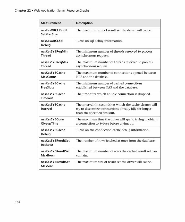
Chapter 22 • Web Application Server Resource Graphs
324
nasKesORCLResultSetMaxSize
The maximum size of result set the driver will cache.
nasKesORCLSqlDebug
Turns on sql debug information.
nasKesSYBReqMinThread
The minimum number of threads reserved to process asynchronous requests.
nasKesSYBReqMaxThread
The maximum number of threads reserved to process asynchronous request.
nasKesSYBCacheMaxConns
The maximum number of connections opened between NAS and the database.
nasKesSYBCacheFreeSlots
The minimum number of cached connections established between NAS and the database.
nasKesSYBCacheTimeout
The time after which an idle connection is dropped.
nasKesSYBCacheInterval
The interval (in seconds) at which the cache cleaner will try to disconnect connections already idle for longer than the specified timeout.
nasKesSYBConnGiveupTime
The maximum time the driver will spend trying to obtain a connection to Sybase before giving up.
nasKesSYBCacheDebug
Turns on the connection cache debug information.
nasKesSYBResultSetInitRows
The number of rows fetched at once from the database.
nasKesSYBResultSetMaxRows
The maximum number of rows the cached result set can contain.
nasKesSYBResultSetMaxSize
The maximum size of result set the driver will cache.
Measurement Description
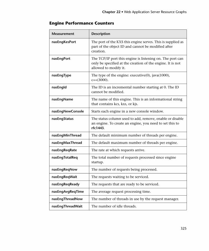
Chapter 22 • Web Application Server Resource Graphs
325
Engine Performance Counters
Measurement Description
nasEngKesPort The port of the KXS this engine serves. This is supplied as part of the object ID and cannot be modified after creation.
nasEngPort The TCP/IP port this engine is listening on. The port can only be specified at the creation of the engine. It is not allowed to modify it.
nasEngType The type of the engine: executive(0), java(1000), c++(3000).
nasEngId The ID is an incremental number starting at 0. The ID cannot be modified.
nasEngName The name of this engine. This is an informational string that contains kcs, kxs, or kjs.
nasEngNewConsole Starts each engine in a new console window.
nasEngStatus The status column used to add, remove, enable or disable an engine. To create an engine, you need to set this to rfc1443.
nasEngMinThread The default minimum number of threads per engine.
nasEngMaxThread The default maximum number of threads per engine.
nasEngReqRate The rate at which requests arrive.
nasEngTotalReq The total number of requests processed since engine startup.
nasEngReqNow The number of requests being processed.
nasEngReqWait The requests waiting to be serviced.
nasEngReqReady The requests that are ready to be serviced.
nasEngAvgReqTime The average request processing time.
nasEngThreadNow The number of threads in use by the request manager.
nasEngThreadWait The number of idle threads.
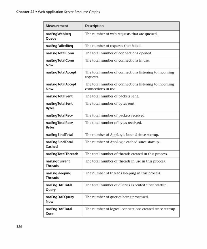
Chapter 22 • Web Application Server Resource Graphs
326
nasEngWebReqQueue
The number of web requests that are queued.
nasEngFailedReq The number of requests that failed.
nasEngTotalConn The total number of connections opened.
nasEngTotalConnNow
The total number of connections in use.
nasEngTotalAccept The total number of connections listening to incoming requests.
nasEngTotalAcceptNow
The total number of connections listening to incoming connections in use.
nasEngTotalSent The total number of packets sent.
nasEngTotalSentBytes
The total number of bytes sent.
nasEngTotalRecv The total number of packets received.
nasEngTotalRecvBytes
The total number of bytes received.
nasEngBindTotal The number of AppLogic bound since startup.
nasEngBindTotalCached
The number of AppLogic cached since startup.
nasEngTotalThreads The total number of threads created in this process.
nasEngCurrentThreads
The total number of threads in use in this process.
nasEngSleepingThreads
The number of threads sleeping in this process.
nasEngDAETotalQuery
The total number of queries executed since startup.
nasEngDAEQueryNow
The number of queries being processed.
nasEngDAETotalConn
The number of logical connections created since startup.
Measurement Description
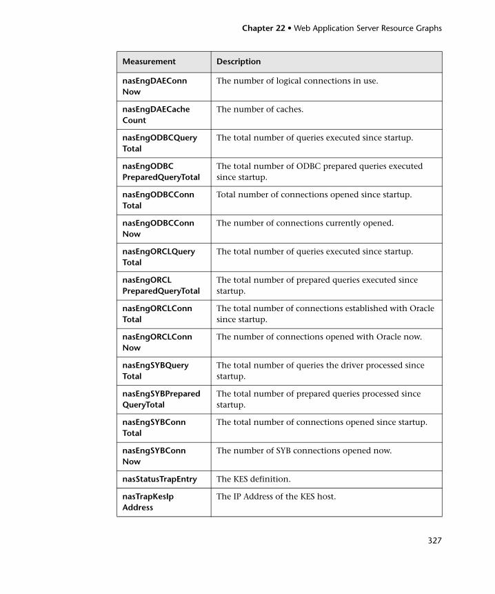
Chapter 22 • Web Application Server Resource Graphs
327
nasEngDAEConnNow
The number of logical connections in use.
nasEngDAECacheCount
The number of caches.
nasEngODBCQueryTotal
The total number of queries executed since startup.
nasEngODBCPreparedQueryTotal
The total number of ODBC prepared queries executed since startup.
nasEngODBCConnTotal
Total number of connections opened since startup.
nasEngODBCConnNow
The number of connections currently opened.
nasEngORCLQueryTotal
The total number of queries executed since startup.
nasEngORCLPreparedQueryTotal
The total number of prepared queries executed since startup.
nasEngORCLConnTotal
The total number of connections established with Oracle since startup.
nasEngORCLConnNow
The number of connections opened with Oracle now.
nasEngSYBQueryTotal
The total number of queries the driver processed since startup.
nasEngSYBPreparedQueryTotal
The total number of prepared queries processed since startup.
nasEngSYBConnTotal
The total number of connections opened since startup.
nasEngSYBConnNow
The number of SYB connections opened now.
nasStatusTrapEntry The KES definition.
nasTrapKesIpAddress
The IP Address of the KES host.
Measurement Description
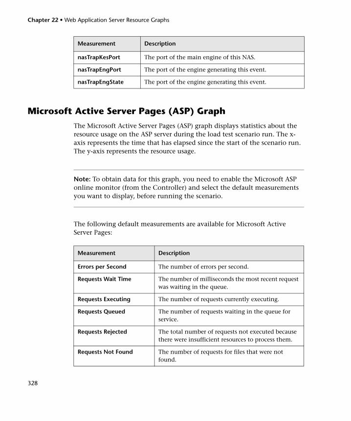
Chapter 22 • Web Application Server Resource Graphs
328
Microsoft Active Server Pages (ASP) Graph
The Microsoft Active Server Pages (ASP) graph displays statistics about the resource usage on the ASP server during the load test scenario run. The x-axis represents the time that has elapsed since the start of the scenario run. The y-axis represents the resource usage.
Note: To obtain data for this graph, you need to enable the Microsoft ASP online monitor (from the Controller) and select the default measurements you want to display, before running the scenario.
The following default measurements are available for Microsoft Active Server Pages:
nasTrapKesPort The port of the main engine of this NAS.
nasTrapEngPort The port of the engine generating this event.
nasTrapEngState The port of the engine generating this event.
Measurement Description
Errors per Second The number of errors per second.
Requests Wait Time The number of milliseconds the most recent request was waiting in the queue.
Requests Executing The number of requests currently executing.
Requests Queued The number of requests waiting in the queue for service.
Requests Rejected The total number of requests not executed because there were insufficient resources to process them.
Requests Not Found The number of requests for files that were not found.
Measurement Description
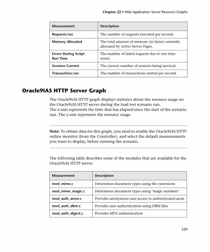
Chapter 22 • Web Application Server Resource Graphs
329
Oracle9iAS HTTP Server Graph
The Oracle9iAS HTTP graph displays statistics about the resource usage on the Oracle9iAS HTTP server during the load test scenario run.The x-axis represents the time that has elapsed since the start of the scenario run. The y-axis represents the resource usage.
Note: To obtain data for this graph, you need to enable the Oracle9iAS HTTP online monitor (from the Controller), and select the default measurements you want to display, before running the scenario.
The following table describes some of the modules that are available for the Oracle9iAS HTTP server:
Requests/sec The number of requests executed per second.
Memory Allocated The total amount of memory (in bytes) currently allocated by Active Server Pages.
Errors During Script Run-Time
The number of failed requests due to run time errors.
Sessions Current The current number of sessions being serviced.
Transactions/sec The number of transactions started per second.
Measurement Description
mod_mime.c Determines document types using file extensions
mod_mime_magic.c Determines document types using "magic numbers"
mod_auth_anon.c Provides anonymous user access to authenticated areas
mod_auth_dbm.c Provides user authentication using DBM files
mod_auth_digest.c Provides MD5 authentication
Measurement Description
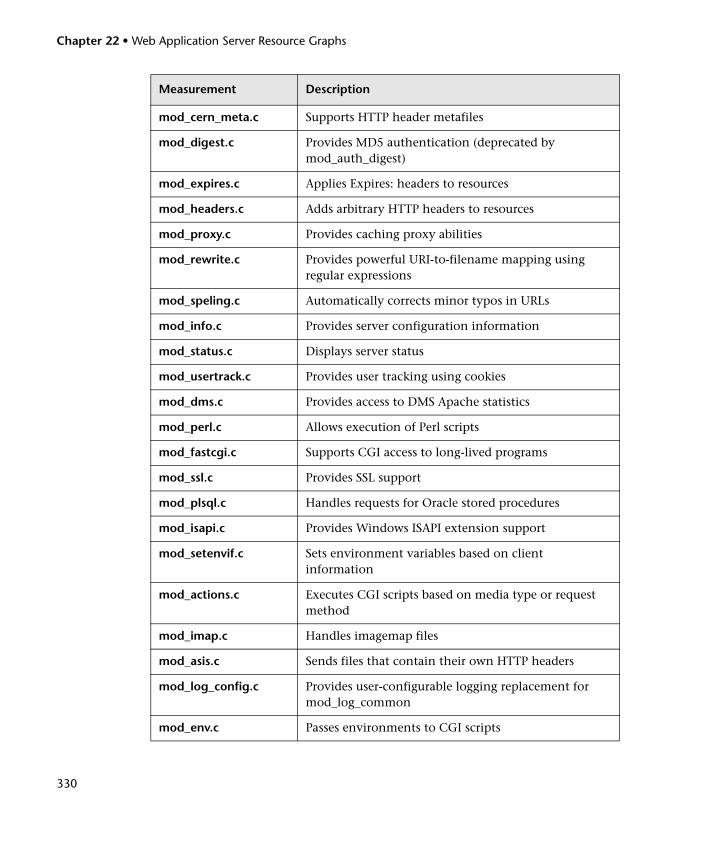
Chapter 22 • Web Application Server Resource Graphs
330
mod_cern_meta.c Supports HTTP header metafiles
mod_digest.c Provides MD5 authentication (deprecated by mod_auth_digest)
mod_expires.c Applies Expires: headers to resources
mod_headers.c Adds arbitrary HTTP headers to resources
mod_proxy.c Provides caching proxy abilities
mod_rewrite.c Provides powerful URI-to-filename mapping using regular expressions
mod_speling.c Automatically corrects minor typos in URLs
mod_info.c Provides server configuration information
mod_status.c Displays server status
mod_usertrack.c Provides user tracking using cookies
mod_dms.c Provides access to DMS Apache statistics
mod_perl.c Allows execution of Perl scripts
mod_fastcgi.c Supports CGI access to long-lived programs
mod_ssl.c Provides SSL support
mod_plsql.c Handles requests for Oracle stored procedures
mod_isapi.c Provides Windows ISAPI extension support
mod_setenvif.c Sets environment variables based on client information
mod_actions.c Executes CGI scripts based on media type or request method
mod_imap.c Handles imagemap files
mod_asis.c Sends files that contain their own HTTP headers
mod_log_config.c Provides user-configurable logging replacement for mod_log_common
mod_env.c Passes environments to CGI scripts
Measurement Description
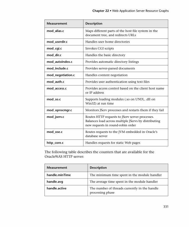
Chapter 22 • Web Application Server Resource Graphs
331
The following table describes the counters that are available for the Oracle9iAS HTTP server:
mod_alias.c Maps different parts of the host file system in the document tree, and redirects URLs
mod_userdir.c Handles user home directories
mod_cgi.c Invokes CGI scripts
mod_dir.c Handles the basic directory
mod_autoindex.c Provides automatic directory listings
mod_include.c Provides server-parsed documents
mod_negotiation.c Handles content negotiation
mod_auth.c Provides user authentication using text files
mod_access.c Provides access control based on the client host name or IP address
mod_so.c Supports loading modules (.so on UNIX, .dll on Win32) at run time
mod_oprocmgr.c Monitors JServ processes and restarts them if they fail
mod_jserv.c Routes HTTP requests to JServ server processes. Balances load across multiple JServs by distributing new requests in round-robin order
mod_ose.c Routes requests to the JVM embedded in Oracle’s database server
http_core.c Handles requests for static Web pages
Measurement Description
handle.minTime The minimum time spent in the module handler
handle.avg The average time spent in the module handler
handle.active The number of threads currently in the handle processing phase
Measurement Description
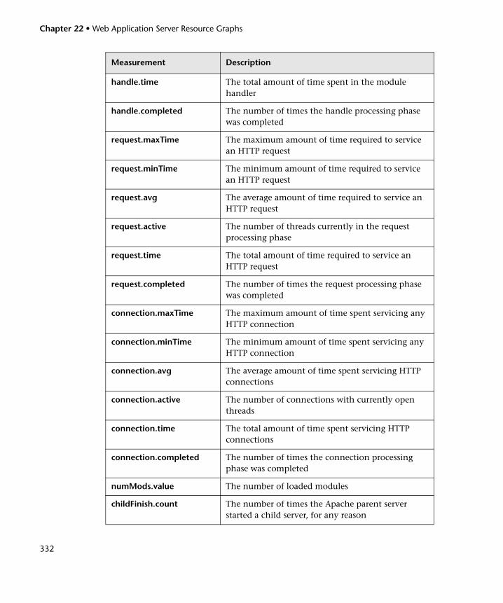
Chapter 22 • Web Application Server Resource Graphs
332
handle.time The total amount of time spent in the module handler
handle.completed The number of times the handle processing phase was completed
request.maxTime The maximum amount of time required to service an HTTP request
request.minTime The minimum amount of time required to service an HTTP request
request.avg The average amount of time required to service an HTTP request
request.active The number of threads currently in the request processing phase
request.time The total amount of time required to service an HTTP request
request.completed The number of times the request processing phase was completed
connection.maxTime The maximum amount of time spent servicing any HTTP connection
connection.minTime The minimum amount of time spent servicing any HTTP connection
connection.avg The average amount of time spent servicing HTTP connections
connection.active The number of connections with currently open threads
connection.time The total amount of time spent servicing HTTP connections
connection.completed The number of times the connection processing phase was completed
numMods.value The number of loaded modules
childFinish.count The number of times the Apache parent server started a child server, for any reason
Measurement Description
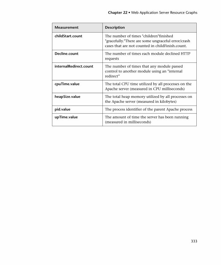
Chapter 22 • Web Application Server Resource Graphs
333
childStart.count The number of times "children"finished "gracefully."There are some ungraceful error/crash cases that are not counted in childFinish.count.
Decline.count The number of times each module declined HTTP requests
internalRedirect.count The number of times that any module passed control to another module using an "internal redirect”
cpuTime.value The total CPU time utilized by all processes on the Apache server (measured in CPU milliseconds)
heapSize.value The total heap memory utilized by all processes on the Apache server (measured in kilobytes)
pid.value The process identifier of the parent Apache process
upTime.value The amount of time the server has been running (measured in milliseconds)
Measurement Description
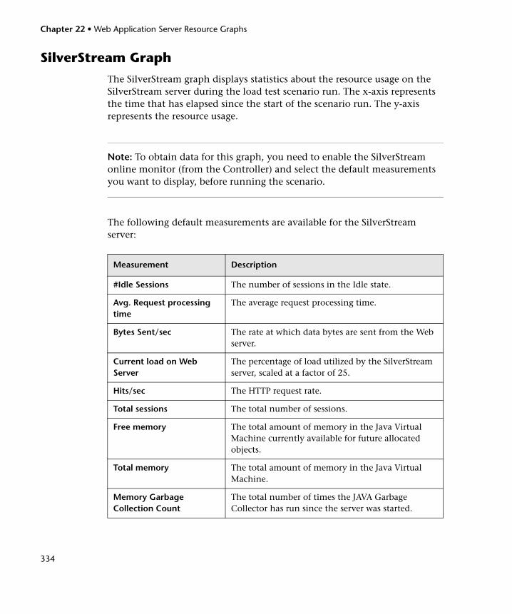
Chapter 22 • Web Application Server Resource Graphs
334
SilverStream Graph
The SilverStream graph displays statistics about the resource usage on the SilverStream server during the load test scenario run. The x-axis represents the time that has elapsed since the start of the scenario run. The y-axis represents the resource usage.
Note: To obtain data for this graph, you need to enable the SilverStream online monitor (from the Controller) and select the default measurements you want to display, before running the scenario.
The following default measurements are available for the SilverStream server:
Measurement Description
#Idle Sessions The number of sessions in the Idle state.
Avg. Request processing time
The average request processing time.
Bytes Sent/sec The rate at which data bytes are sent from the Web server.
Current load on Web Server
The percentage of load utilized by the SilverStream server, scaled at a factor of 25.
Hits/sec The HTTP request rate.
Total sessions The total number of sessions.
Free memory The total amount of memory in the Java Virtual Machine currently available for future allocated objects.
Total memory The total amount of memory in the Java Virtual Machine.
Memory Garbage Collection Count
The total number of times the JAVA Garbage Collector has run since the server was started.
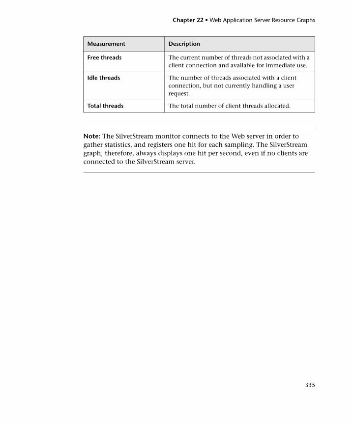
Chapter 22 • Web Application Server Resource Graphs
335
Note: The SilverStream monitor connects to the Web server in order to gather statistics, and registers one hit for each sampling. The SilverStream graph, therefore, always displays one hit per second, even if no clients are connected to the SilverStream server.
Free threads The current number of threads not associated with a client connection and available for immediate use.
Idle threads The number of threads associated with a client connection, but not currently handling a user request.
Total threads The total number of client threads allocated.
Measurement Description
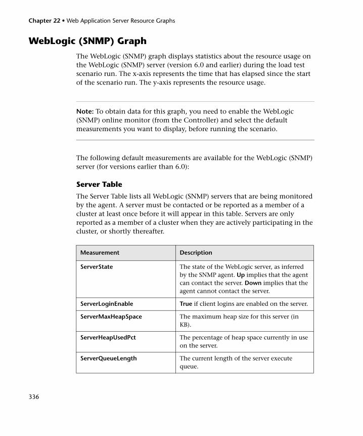
Chapter 22 • Web Application Server Resource Graphs
336
WebLogic (SNMP) Graph
The WebLogic (SNMP) graph displays statistics about the resource usage on the WebLogic (SNMP) server (version 6.0 and earlier) during the load test scenario run. The x-axis represents the time that has elapsed since the start of the scenario run. The y-axis represents the resource usage.
Note: To obtain data for this graph, you need to enable the WebLogic (SNMP) online monitor (from the Controller) and select the default measurements you want to display, before running the scenario.
The following default measurements are available for the WebLogic (SNMP) server (for versions earlier than 6.0):
Server Table
The Server Table lists all WebLogic (SNMP) servers that are being monitored by the agent. A server must be contacted or be reported as a member of a cluster at least once before it will appear in this table. Servers are only reported as a member of a cluster when they are actively participating in the cluster, or shortly thereafter.
Measurement Description
ServerState The state of the WebLogic server, as inferred by the SNMP agent. Up implies that the agent can contact the server. Down implies that the agent cannot contact the server.
ServerLoginEnable True if client logins are enabled on the server.
ServerMaxHeapSpace The maximum heap size for this server (in KB).
ServerHeapUsedPct The percentage of heap space currently in use on the server.
ServerQueueLength The current length of the server execute queue.
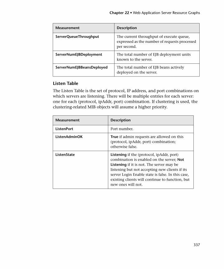
Chapter 22 • Web Application Server Resource Graphs
337
Listen Table
The Listen Table is the set of protocol, IP address, and port combinations on which servers are listening. There will be multiple entries for each server: one for each (protocol, ipAddr, port) combination. If clustering is used, the clustering-related MIB objects will assume a higher priority.
ServerQueueThroughput The current throughput of execute queue, expressed as the number of requests processed per second.
ServerNumEJBDeployment The total number of EJB deployment units known to the server.
ServerNumEJBBeansDeployed The total number of EJB beans actively deployed on the server.
Measurement Description
ListenPort Port number.
ListenAdminOK True if admin requests are allowed on this (protocol, ipAddr, port) combination; otherwise false.
ListenState Listening if the (protocol, ipAddr, port) combination is enabled on the server; Not Listening if it is not. The server may be listening but not accepting new clients if its server Login Enable state is false. In this case, existing clients will continue to function, but new ones will not.
Measurement Description
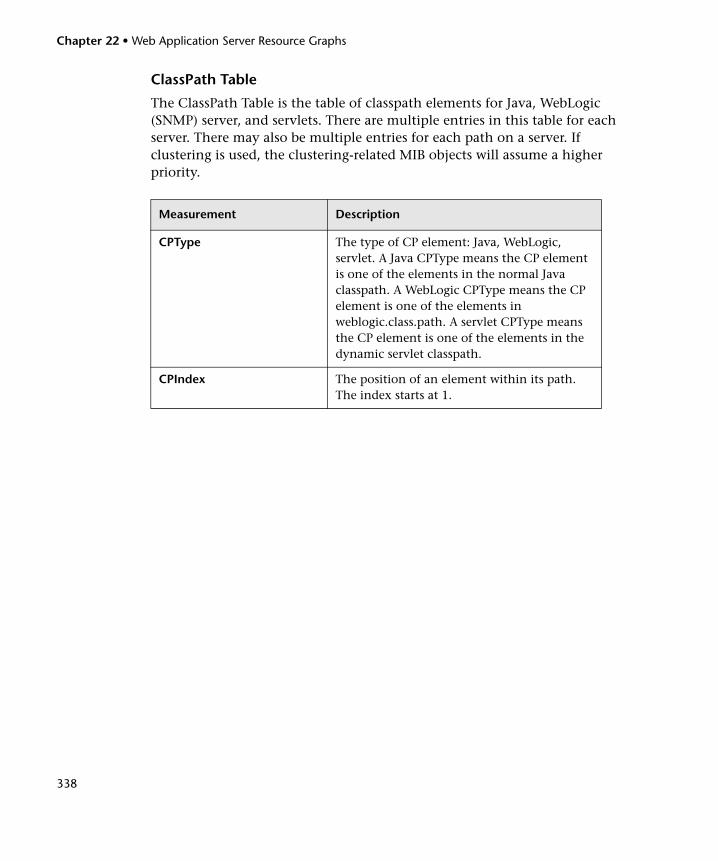
Chapter 22 • Web Application Server Resource Graphs
338
ClassPath Table
The ClassPath Table is the table of classpath elements for Java, WebLogic (SNMP) server, and servlets. There are multiple entries in this table for each server. There may also be multiple entries for each path on a server. If clustering is used, the clustering-related MIB objects will assume a higher priority.
Measurement Description
CPType The type of CP element: Java, WebLogic, servlet. A Java CPType means the CP element is one of the elements in the normal Java classpath. A WebLogic CPType means the CP element is one of the elements in weblogic.class.path. A servlet CPType means the CP element is one of the elements in the dynamic servlet classpath.
CPIndex The position of an element within its path. The index starts at 1.
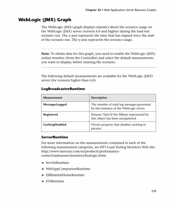
Chapter 22 • Web Application Server Resource Graphs
339
WebLogic (JMX) Graph
The WebLogic (JMX) graph displays statistics about the resource usage on the WebLogic (JMX) server (version 6.0 and higher) during the load test scenario run. The x-axis represents the time that has elapsed since the start of the scenario run. The y-axis represents the resource usage.
Note: To obtain data for this graph, you need to enable the WebLogic (JMX) online monitor (from the Controller) and select the default measurements you want to display, before running the scenario.
The following default measurements are available for the WebLogic (JMX) server (for versions higher than 6.0):
LogBroadcasterRuntime
ServerRuntime
For more information on the measurements contained in each of the following measurement categories, see HP’s Load Testing Monitors Web site: http://www.mercury.com/us/products/performance-center/loadrunner/monitors/bealogic.html.
➤ ServletRuntime
➤ WebAppComponentRuntime
➤ EJBStatefulHomeRuntime
➤ JTARuntime
Measurement Description
MessagesLogged The number of total log messages generated by this instance of the WebLogic server.
Registered Returns "false"if the MBean represented by this object has been unregistered.
CachingDisabled Private property that disables caching in proxies.
Chapter 22 • Web Application Server Resource Graphs
340
➤ JVMRuntime
➤ EJBEntityHomeRuntime
➤ DomainRuntime
➤ EJBComponentRuntime
➤ DomainLogHandlerRuntime
➤ JDBCConnectionPoolRuntime
➤ ExecuteQueueRuntime
➤ ClusterRuntime
➤ JMSRuntime
➤ TimeServiceRuntime
➤ EJBStatelessHomeRuntime
➤ WLECConnectionServiceRuntime

Chapter 22 • Web Application Server Resource Graphs
341
ServerSecurityRuntime
Measurement Description
UnlockedUsersTotalCount Returns the number of times a user has been unlocked on the server.
InvalidLoginUsersHighCount Returns the high-water number of users with outstanding invalid login attempts for the server.
LoginAttemptsWhileLockedTotalCount Returns the cumulative number of invalid logins attempted on the server while the user was locked.
Registered Returns False if the MBean represented by this object has been unregistered.
LockedUsersCurrentCount Returns the number of currently locked users on the server.
CachingDisabled Private property that disables caching in proxies.
InvalidLoginAttemptsTotalCount Returns the cumulative number of invalid logins attempted on the server.
UserLockoutTotalCount Returns the cumulative number of user lockouts that occurred on the server.
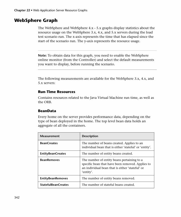
Chapter 22 • Web Application Server Resource Graphs
342
WebSphere Graph
The WebSphere and WebSphere 4.x - 5.x graphs display statistics about the resource usage on the WebSphere 3.x, 4.x, and 5.x servers during the load test scenario run. The x-axis represents the time that has elapsed since the start of the scenario run. The y-axis represents the resource usage.
Note: To obtain data for this graph, you need to enable the WebSphere online monitor (from the Controller) and select the default measurements you want to display, before running the scenario.
The following measurements are available for the WebSphere 3.x, 4.x, and 5.x servers:
Run-Time Resources
Contains resources related to the Java Virtual Machine run time, as well as the ORB.
BeanData
Every home on the server provides performance data, depending on the type of bean deployed in the home. The top level bean data holds an aggregate of all the containers.
Measurement Description
BeanCreates The number of beans created. Applies to an individual bean that is either ‘stateful’ or ‘entity’.
EntityBeanCreates The number of entity beans created.
BeanRemoves The number of entity beans pertaining to a specific bean that have been removed. Applies to an individual bean that is either ‘stateful’ or ‘entity’.
EntityBeanRemoves The number of entity beans removed.
StatefulBeanCreates The number of stateful beans created.
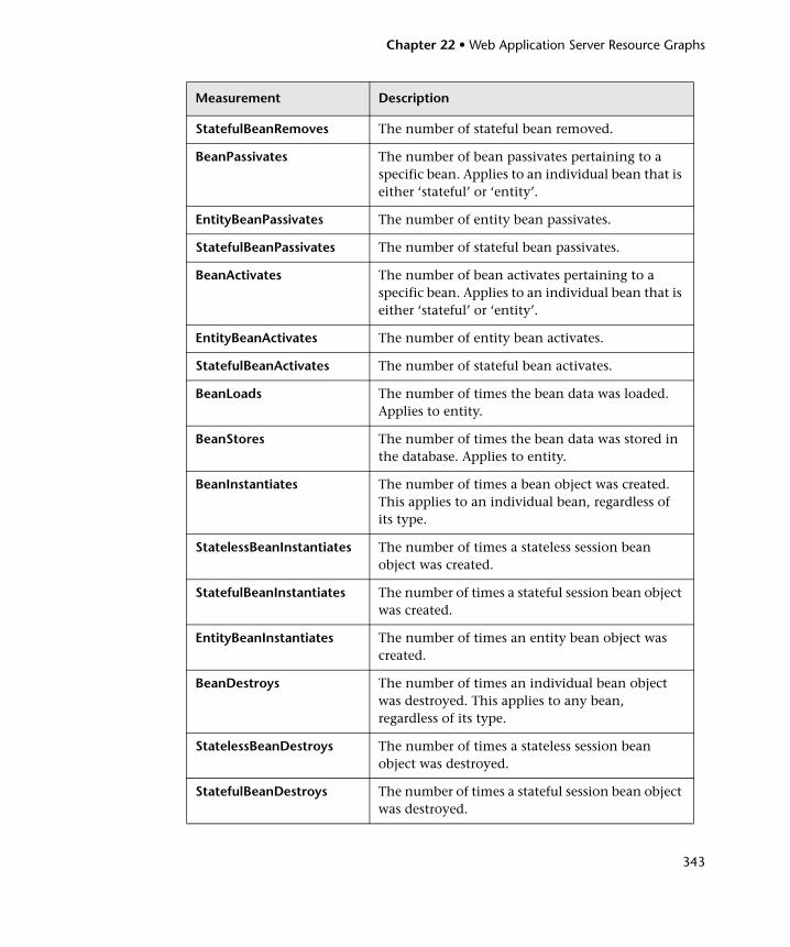
Chapter 22 • Web Application Server Resource Graphs
343
StatefulBeanRemoves The number of stateful bean removed.
BeanPassivates The number of bean passivates pertaining to a specific bean. Applies to an individual bean that is either ‘stateful’ or ‘entity’.
EntityBeanPassivates The number of entity bean passivates.
StatefulBeanPassivates The number of stateful bean passivates.
BeanActivates The number of bean activates pertaining to a specific bean. Applies to an individual bean that is either ‘stateful’ or ‘entity’.
EntityBeanActivates The number of entity bean activates.
StatefulBeanActivates The number of stateful bean activates.
BeanLoads The number of times the bean data was loaded. Applies to entity.
BeanStores The number of times the bean data was stored in the database. Applies to entity.
BeanInstantiates The number of times a bean object was created. This applies to an individual bean, regardless of its type.
StatelessBeanInstantiates The number of times a stateless session bean object was created.
StatefulBeanInstantiates The number of times a stateful session bean object was created.
EntityBeanInstantiates The number of times an entity bean object was created.
BeanDestroys The number of times an individual bean object was destroyed. This applies to any bean, regardless of its type.
StatelessBeanDestroys The number of times a stateless session bean object was destroyed.
StatefulBeanDestroys The number of times a stateful session bean object was destroyed.
Measurement Description
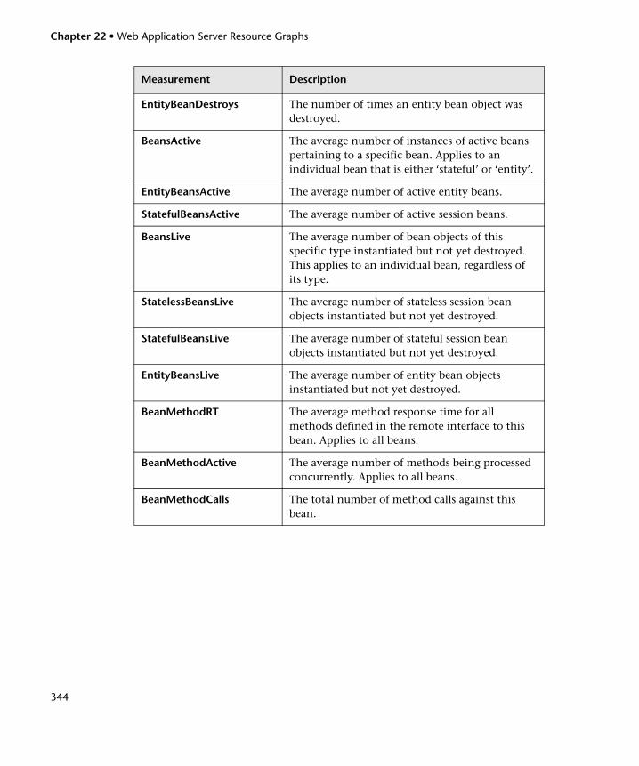
Chapter 22 • Web Application Server Resource Graphs
344
EntityBeanDestroys The number of times an entity bean object was destroyed.
BeansActive The average number of instances of active beans pertaining to a specific bean. Applies to an individual bean that is either ‘stateful’ or ‘entity’.
EntityBeansActive The average number of active entity beans.
StatefulBeansActive The average number of active session beans.
BeansLive The average number of bean objects of this specific type instantiated but not yet destroyed. This applies to an individual bean, regardless of its type.
StatelessBeansLive The average number of stateless session bean objects instantiated but not yet destroyed.
StatefulBeansLive The average number of stateful session bean objects instantiated but not yet destroyed.
EntityBeansLive The average number of entity bean objects instantiated but not yet destroyed.
BeanMethodRT The average method response time for all methods defined in the remote interface to this bean. Applies to all beans.
BeanMethodActive The average number of methods being processed concurrently. Applies to all beans.
BeanMethodCalls The total number of method calls against this bean.
Measurement Description
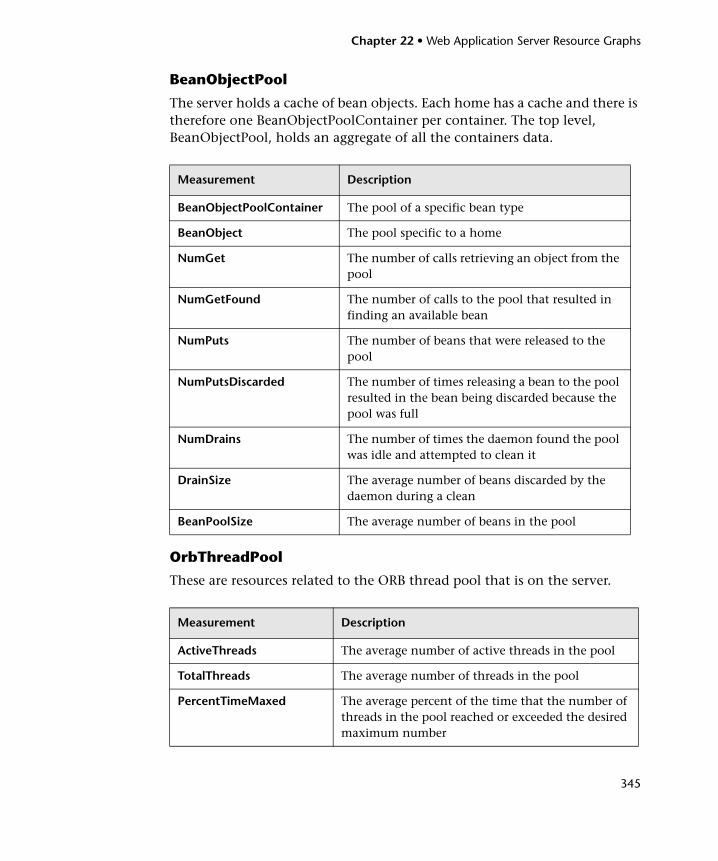
Chapter 22 • Web Application Server Resource Graphs
345
BeanObjectPool
The server holds a cache of bean objects. Each home has a cache and there is therefore one BeanObjectPoolContainer per container. The top level, BeanObjectPool, holds an aggregate of all the containers data.
OrbThreadPool
These are resources related to the ORB thread pool that is on the server.
Measurement Description
BeanObjectPoolContainer The pool of a specific bean type
BeanObject The pool specific to a home
NumGet The number of calls retrieving an object from the pool
NumGetFound The number of calls to the pool that resulted in finding an available bean
NumPuts The number of beans that were released to the pool
NumPutsDiscarded The number of times releasing a bean to the pool resulted in the bean being discarded because the pool was full
NumDrains The number of times the daemon found the pool was idle and attempted to clean it
DrainSize The average number of beans discarded by the daemon during a clean
BeanPoolSize The average number of beans in the pool
Measurement Description
ActiveThreads The average number of active threads in the pool
TotalThreads The average number of threads in the pool
PercentTimeMaxed The average percent of the time that the number of threads in the pool reached or exceeded the desired maximum number
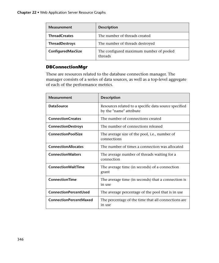
Chapter 22 • Web Application Server Resource Graphs
346
DBConnectionMgr
These are resources related to the database connection manager. The manager consists of a series of data sources, as well as a top-level aggregate of each of the performance metrics.
ThreadCreates The number of threads created
ThreadDestroys The number of threads destroyed
ConfiguredMaxSize The configured maximum number of pooled threads
Measurement Description
DataSource Resources related to a specific data source specified by the "name" attribute
ConnectionCreates The number of connections created
ConnectionDestroys The number of connections released
ConnectionPoolSize The average size of the pool, i.e., number of connections
ConnectionAllocates The number of times a connection was allocated
ConnectionWaiters The average number of threads waiting for a connection
ConnectionWaitTime The average time (in seconds) of a connection grant
ConnectionTime The average time (in seconds) that a connection is in use
ConnectionPercentUsed The average percentage of the pool that is in use
ConnectionPercentMaxed The percentage of the time that all connections are in use
Measurement Description
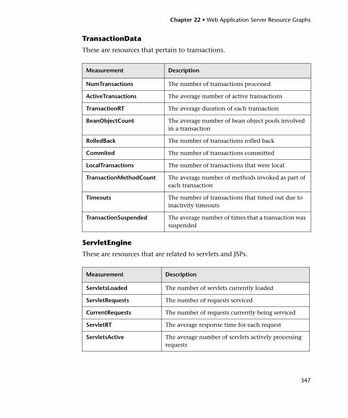
Chapter 22 • Web Application Server Resource Graphs
347
TransactionData
These are resources that pertain to transactions.
ServletEngine
These are resources that are related to servlets and JSPs.
Measurement Description
NumTransactions The number of transactions processed
ActiveTransactions The average number of active transactions
TransactionRT The average duration of each transaction
BeanObjectCount The average number of bean object pools involved in a transaction
RolledBack The number of transactions rolled back
Commited The number of transactions committed
LocalTransactions The number of transactions that were local
TransactionMethodCount The average number of methods invoked as part of each transaction
Timeouts The number of transactions that timed out due to inactivity timeouts
TransactionSuspended The average number of times that a transaction was suspended
Measurement Description
ServletsLoaded The number of servlets currently loaded
ServletRequests The number of requests serviced
CurrentRequests The number of requests currently being serviced
ServletRT The average response time for each request
ServletsActive The average number of servlets actively processing requests
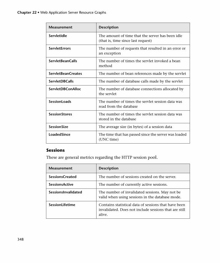
Chapter 22 • Web Application Server Resource Graphs
348
Sessions
These are general metrics regarding the HTTP session pool.
ServletIdle The amount of time that the server has been idle (that is, time since last request)
ServletErrors The number of requests that resulted in an error or an exception
ServletBeanCalls The number of times the servlet invoked a bean method
ServletBeanCreates The number of bean references made by the servlet
ServletDBCalls The number of database calls made by the servlet
ServletDBConAlloc The number of database connections allocated by the servlet
SessionLoads The number of times the servlet session data was read from the database
SessionStores The number of times the servlet session data was stored in the database
SessionSize The average size (in bytes) of a session data
LoadedSince The time that has passed since the server was loaded (UNC time)
Measurement Description
SessionsCreated The number of sessions created on the server.
SessionsActive The number of currently active sessions.
SessionsInvalidated The number of invalidated sessions. May not be valid when using sessions in the database mode.
SessionLifetime Contains statistical data of sessions that have been invalidated. Does not include sessions that are still alive.
Measurement Description
Chapter 22 • Web Application Server Resource Graphs
349
WebSphere Application Server Graph
The WebSphere Application Server graph displays statistics about the resource usage on the WebSphere application server during the load test scenario run. The x-axis represents the time that has elapsed since the start of the scenario or run. The y-axis represents the resource usage.
Note: To obtain data for this graph, you need to configure the WebSphere Application Server online monitor (from the Controller) and select the default measurements you want to display, before running the scenario.
The following measurements are available for the WebSphere Application Server monitor:
Run-Time Resources
Contains resources related to the Java Virtual Machine run time, as well as the ORB.
Measurement Description
MemoryFree The amount of free memory remaining in the Java Virtual Machine
MemoryTotal The total memory allocated for the Java Virtual Machine
MemoryUse The total memory in use on the Java Virtual Machine
Chapter 22 • Web Application Server Resource Graphs
350
BeanData
Every home on the server provides performance data, depending on the type of bean deployed in the home. The top level bean data holds an aggregate of all the containers.
BeanObjectPool
The server holds a cache of bean objects. Each home has a cache and there is therefore one BeanObjectPoolContainer per container. The top level, BeanObjectPool, holds an aggregate of all the containers data.
OrbThreadPool
These are resources related to the ORB thread pool that is on the server.
Measurement Description
BeanDestroys The number of times an individual bean object was destroyed. This applies to any bean, regardless of its type.
StatelessBeanDestroys The number of times a stateless session bean object was destroyed.
StatefulBeanDestroys The number of times a stateful session bean object was destroyed.
Measurement Description
NumGetFound The number of calls to the pool that resulted in finding an available bean
NumPutsDiscarded The number of times releasing a bean to the pool resulted in the bean being discarded because the pool was full
Measurement Description
ActiveThreads The average number of active threads in the pool
Chapter 22 • Web Application Server Resource Graphs
351
DBConnectionMgr
These are resources related to the database connection manager. The manager consists of a series of data sources, as well as a top-level aggregate of each of the performance metrics.
TransactionData
These are resources that pertain to transactions.
TotalThreads The average number of threads in the pool
PercentTimeMaxed The average percent of the time that the number of threads in the pool reached or exceeded the desired maximum number
Measurement Description
ConnectionWaitTime The average time (in seconds) of a connection grant
ConnectionTime The average time (in seconds) that a connection is in use
ConnectionPercentUsed The average percentage of the pool that is in use
Measurement Description
NumTransactions The number of transactions processed
ActiveTransactions The average number of active transactions
TransactionRT The average duration of each transaction
RolledBack The number of transactions rolled back
Timeouts The number of transactions that timed out due to inactivity timeouts
TransactionSuspended The average number of times that a transaction was suspended
Measurement Description
Chapter 22 • Web Application Server Resource Graphs
352
ServletEngine
These are resources that are related to servlets and JSPs.
Sessions
These are general metrics regarding the HTTP session pool.
.
Measurement Description
ServletErrors The number of requests that resulted in an error or an exception
Measurement Description
SessionsInvalidated The number of invalidated sessions. May not be valid when using sessions in the database mode.

Chapter 22 • Web Application Server Resource Graphs
353
WebSphere (EPM) Graph
The WebSphere (EPM) graph displays statistics about the resource usage on the WebSphere 3.5.x server during the load test scenario run.The x-axis represents the time that has elapsed since the start of the scenario run. The y-axis represents the resource usage.
Note: To obtain data for this graph, you need to enable the WebSphere (EPM) online monitor (from the Controller) and select the default measurements you want to display, before running the scenario.
The following measurements are available for the WebSphere (EPM) server:
Run Time Resources
Contains resources related to the Java Virtual Machine run time, as well as the ORB.
Measurement Description
MemoryFree The amount of free memory remaining in the Java Virtual Machine
MemoryTotal The total memory allocated for the Java Virtual Machine
MemoryUse The total memory in use on the Java Virtual Machine
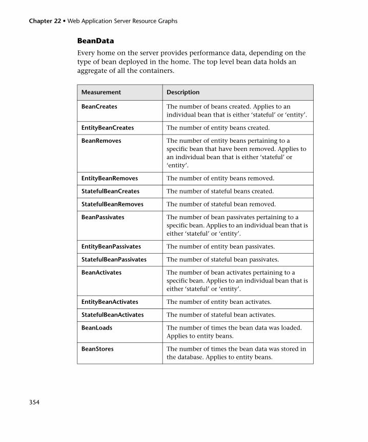
Chapter 22 • Web Application Server Resource Graphs
354
BeanData
Every home on the server provides performance data, depending on the type of bean deployed in the home. The top level bean data holds an aggregate of all the containers.
Measurement Description
BeanCreates The number of beans created. Applies to an individual bean that is either ‘stateful’ or ‘entity’.
EntityBeanCreates The number of entity beans created.
BeanRemoves The number of entity beans pertaining to a specific bean that have been removed. Applies to an individual bean that is either ‘stateful’ or ‘entity’.
EntityBeanRemoves The number of entity beans removed.
StatefulBeanCreates The number of stateful beans created.
StatefulBeanRemoves The number of stateful bean removed.
BeanPassivates The number of bean passivates pertaining to a specific bean. Applies to an individual bean that is either ‘stateful’ or ‘entity’.
EntityBeanPassivates The number of entity bean passivates.
StatefulBeanPassivates The number of stateful bean passivates.
BeanActivates The number of bean activates pertaining to a specific bean. Applies to an individual bean that is either ‘stateful’ or ‘entity’.
EntityBeanActivates The number of entity bean activates.
StatefulBeanActivates The number of stateful bean activates.
BeanLoads The number of times the bean data was loaded. Applies to entity beans.
BeanStores The number of times the bean data was stored in the database. Applies to entity beans.
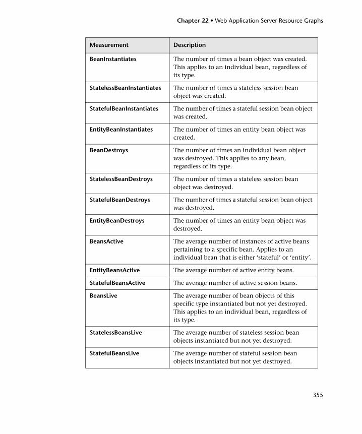
Chapter 22 • Web Application Server Resource Graphs
355
BeanInstantiates The number of times a bean object was created. This applies to an individual bean, regardless of its type.
StatelessBeanInstantiates The number of times a stateless session bean object was created.
StatefulBeanInstantiates The number of times a stateful session bean object was created.
EntityBeanInstantiates The number of times an entity bean object was created.
BeanDestroys The number of times an individual bean object was destroyed. This applies to any bean, regardless of its type.
StatelessBeanDestroys The number of times a stateless session bean object was destroyed.
StatefulBeanDestroys The number of times a stateful session bean object was destroyed.
EntityBeanDestroys The number of times an entity bean object was destroyed.
BeansActive The average number of instances of active beans pertaining to a specific bean. Applies to an individual bean that is either ‘stateful’ or ‘entity’.
EntityBeansActive The average number of active entity beans.
StatefulBeansActive The average number of active session beans.
BeansLive The average number of bean objects of this specific type instantiated but not yet destroyed. This applies to an individual bean, regardless of its type.
StatelessBeansLive The average number of stateless session bean objects instantiated but not yet destroyed.
StatefulBeansLive The average number of stateful session bean objects instantiated but not yet destroyed.
Measurement Description
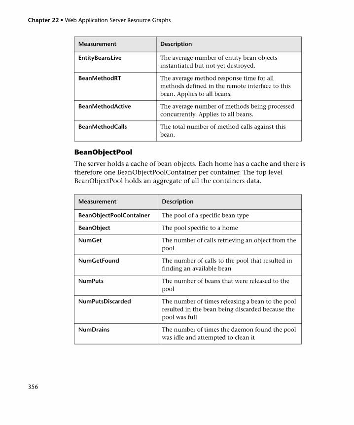
Chapter 22 • Web Application Server Resource Graphs
356
BeanObjectPool
The server holds a cache of bean objects. Each home has a cache and there is therefore one BeanObjectPoolContainer per container. The top level BeanObjectPool holds an aggregate of all the containers data.
EntityBeansLive The average number of entity bean objects instantiated but not yet destroyed.
BeanMethodRT The average method response time for all methods defined in the remote interface to this bean. Applies to all beans.
BeanMethodActive The average number of methods being processed concurrently. Applies to all beans.
BeanMethodCalls The total number of method calls against this bean.
Measurement Description
BeanObjectPoolContainer The pool of a specific bean type
BeanObject The pool specific to a home
NumGet The number of calls retrieving an object from the pool
NumGetFound The number of calls to the pool that resulted in finding an available bean
NumPuts The number of beans that were released to the pool
NumPutsDiscarded The number of times releasing a bean to the pool resulted in the bean being discarded because the pool was full
NumDrains The number of times the daemon found the pool was idle and attempted to clean it
Measurement Description
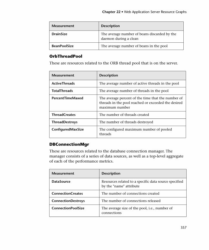
Chapter 22 • Web Application Server Resource Graphs
357
OrbThreadPool
These are resources related to the ORB thread pool that is on the server.
DBConnectionMgr
These are resources related to the database connection manager. The manager consists of a series of data sources, as well as a top-level aggregate of each of the performance metrics.
DrainSize The average number of beans discarded by the daemon during a clean
BeanPoolSize The average number of beans in the pool
Measurement Description
ActiveThreads The average number of active threads in the pool
TotalThreads The average number of threads in the pool
PercentTimeMaxed The average percent of the time that the number of threads in the pool reached or exceeded the desired maximum number
ThreadCreates The number of threads created
ThreadDestroys The number of threads destroyed
ConfiguredMaxSize The configured maximum number of pooled threads
Measurement Description
DataSource Resources related to a specific data source specified by the "name" attribute
ConnectionCreates The number of connections created
ConnectionDestroys The number of connections released
ConnectionPoolSize The average size of the pool, i.e., number of connections
Measurement Description
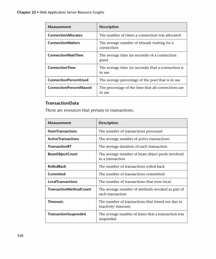
Chapter 22 • Web Application Server Resource Graphs
358
TransactionData
These are resources that pertain to transactions.
ConnectionAllocates The number of times a connection was allocated
ConnectionWaiters The average number of threads waiting for a connection
ConnectionWaitTime The average time (in seconds) of a connection grant
ConnectionTime The average time (in seconds) that a connection is in use
ConnectionPercentUsed The average percentage of the pool that is in use
ConnectionPercentMaxed The percentage of the time that all connections are in use
Measurement Description
NumTransactions The number of transactions processed
ActiveTransactions The average number of active transactions
TransactionRT The average duration of each transaction
BeanObjectCount The average number of bean object pools involved in a transaction
RolledBack The number of transactions rolled back
Commited The number of transactions committed
LocalTransactions The number of transactions that were local
TransactionMethodCount The average number of methods invoked as part of each transaction
Timeouts The number of transactions that timed out due to inactivity timeouts
TransactionSuspended The average number of times that a transaction was suspended
Measurement Description
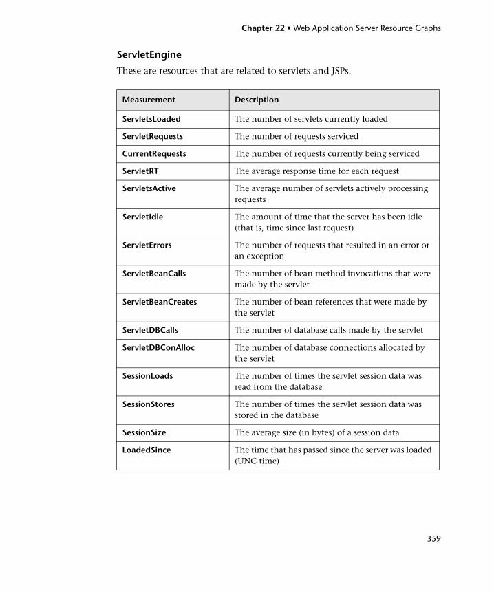
Chapter 22 • Web Application Server Resource Graphs
359
ServletEngine
These are resources that are related to servlets and JSPs.
Measurement Description
ServletsLoaded The number of servlets currently loaded
ServletRequests The number of requests serviced
CurrentRequests The number of requests currently being serviced
ServletRT The average response time for each request
ServletsActive The average number of servlets actively processing requests
ServletIdle The amount of time that the server has been idle (that is, time since last request)
ServletErrors The number of requests that resulted in an error or an exception
ServletBeanCalls The number of bean method invocations that were made by the servlet
ServletBeanCreates The number of bean references that were made by the servlet
ServletDBCalls The number of database calls made by the servlet
ServletDBConAlloc The number of database connections allocated by the servlet
SessionLoads The number of times the servlet session data was read from the database
SessionStores The number of times the servlet session data was stored in the database
SessionSize The average size (in bytes) of a session data
LoadedSince The time that has passed since the server was loaded (UNC time)
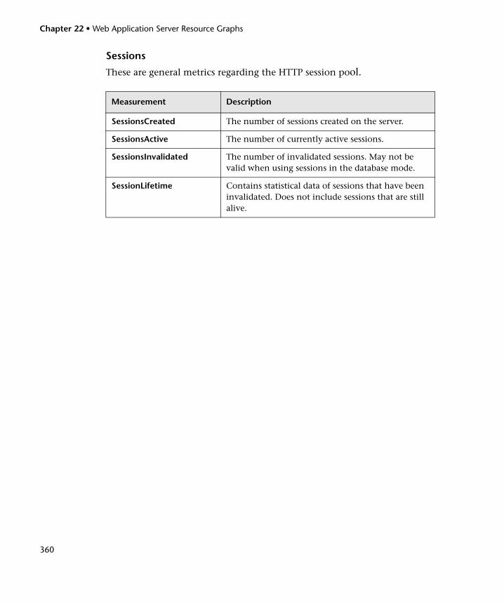
Chapter 22 • Web Application Server Resource Graphs
360
Sessions
These are general metrics regarding the HTTP session pool.
Measurement Description
SessionsCreated The number of sessions created on the server.
SessionsActive The number of currently active sessions.
SessionsInvalidated The number of invalidated sessions. May not be valid when using sessions in the database mode.
SessionLifetime Contains statistical data of sessions that have been invalidated. Does not include sessions that are still alive.
361
23 Database Server Resource Graphs
After running a load test scenario, you can use Database Server Resource graphs to analyze the resource usage of your DB2, Oracle, SQL server, and Sybase databases.
This chapter includes:
➤ About Database Server Resource Graphs on page 361
➤ DB2 Graph on page 362
➤ Oracle Graph on page 377
➤ SQL Server Graph on page 380
➤ Sybase Graph on page 382
About Database Server Resource Graphs
The Database Server Resource graphs show statistics for several database servers. Currently DB2, Oracle, SQL server, and Sybase databases are supported. These graphs require that you specify the resources you want to measure before running the load test scenario. For more information, refer to the section on online monitors in the HP LoadRunner Controller User Guide.

Chapter 23 • Database Server Resource Graphs
362
DB2 Graph
The DB2 graph shows the resource usage on the DB2 database server machine as a function of the elapsed load test scenario time. The x-axis represents the time that has elapsed since the start of the scenario run. The y-axis represents the resource usage.
Note: In order to monitor the DB2 database server machine, you must first set up the DB2 monitor environment. You then enable the DB2 monitor (from the Controller) by selecting the counters you want the monitor to measure.
The following tables describe the default counters that can be monitored on a DB2 server:
DatabaseManager
Measurement Description
rem_cons_in The current number of connections initiated from remote clients to the instance of the database manager that is being monitored.
rem_cons_in_exec The number of remote applications that are currently connected to a database and are currently processing a unit of work within the database manager instance being monitored.
local_cons The number of local applications that are currently connected to a database within the database manager instance being monitored.
local_cons_in_exec The number of local applications that are currently connected to a database within the database manager instance being monitored and are currently processing a unit of work.
con_local_dbases The number of local databases that have applications connected.
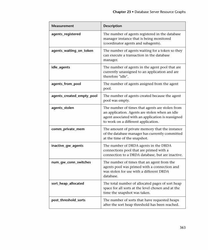
Chapter 23 • Database Server Resource Graphs
363
agents_registered The number of agents registered in the database manager instance that is being monitored (coordinator agents and subagents).
agents_waiting_on_token The number of agents waiting for a token so they can execute a transaction in the database manager.
idle_agents The number of agents in the agent pool that are currently unassigned to an application and are therefore "idle".
agents_from_pool The number of agents assigned from the agent pool.
agents_created_empty_pool The number of agents created because the agent pool was empty.
agents_stolen The number of times that agents are stolen from an application. Agents are stolen when an idle agent associated with an application is reassigned to work on a different application.
comm_private_mem The amount of private memory that the instance of the database manager has currently committed at the time of the snapshot.
inactive_gw_agents The number of DRDA agents in the DRDA connections pool that are primed with a connection to a DRDA database, but are inactive.
num_gw_conn_switches The number of times that an agent from the agents pool was primed with a connection and was stolen for use with a different DRDA database.
sort_heap_allocated The total number of allocated pages of sort heap space for all sorts at the level chosen and at the time the snapshot was taken.
post_threshold_sorts The number of sorts that have requested heaps after the sort heap threshold has been reached.
Measurement Description
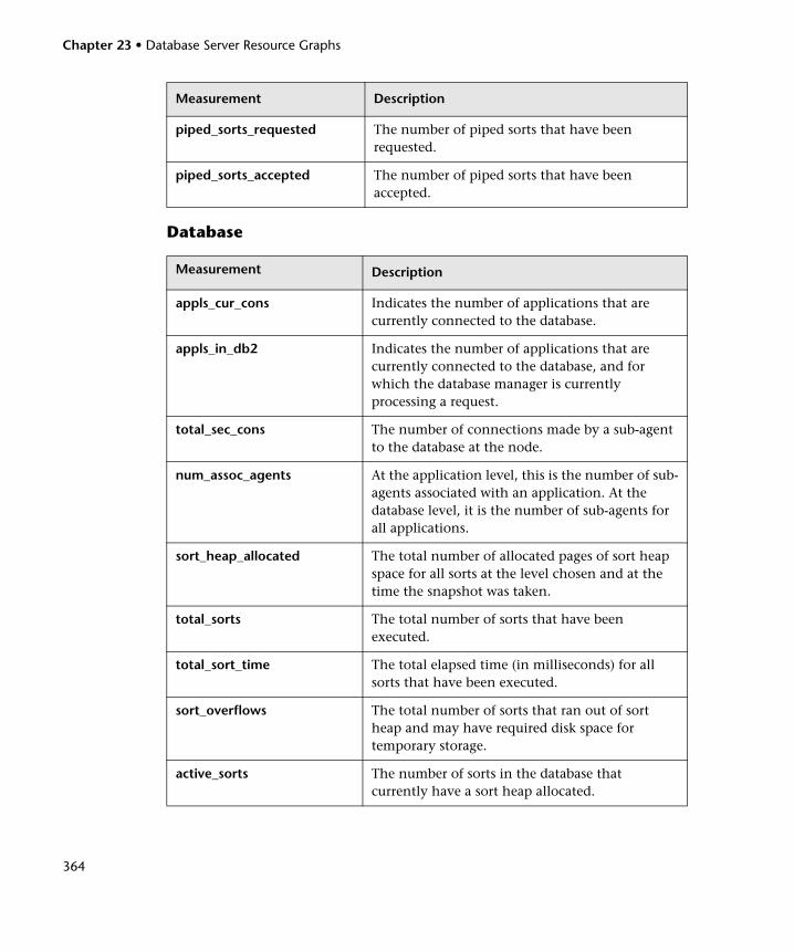
Chapter 23 • Database Server Resource Graphs
364
Database
piped_sorts_requested The number of piped sorts that have been requested.
piped_sorts_accepted The number of piped sorts that have been accepted.
Measurement Description
appls_cur_cons Indicates the number of applications that are currently connected to the database.
appls_in_db2 Indicates the number of applications that are currently connected to the database, and for which the database manager is currently processing a request.
total_sec_cons The number of connections made by a sub-agent to the database at the node.
num_assoc_agents At the application level, this is the number of sub-agents associated with an application. At the database level, it is the number of sub-agents for all applications.
sort_heap_allocated The total number of allocated pages of sort heap space for all sorts at the level chosen and at the time the snapshot was taken.
total_sorts The total number of sorts that have been executed.
total_sort_time The total elapsed time (in milliseconds) for all sorts that have been executed.
sort_overflows The total number of sorts that ran out of sort heap and may have required disk space for temporary storage.
active_sorts The number of sorts in the database that currently have a sort heap allocated.
Measurement Description
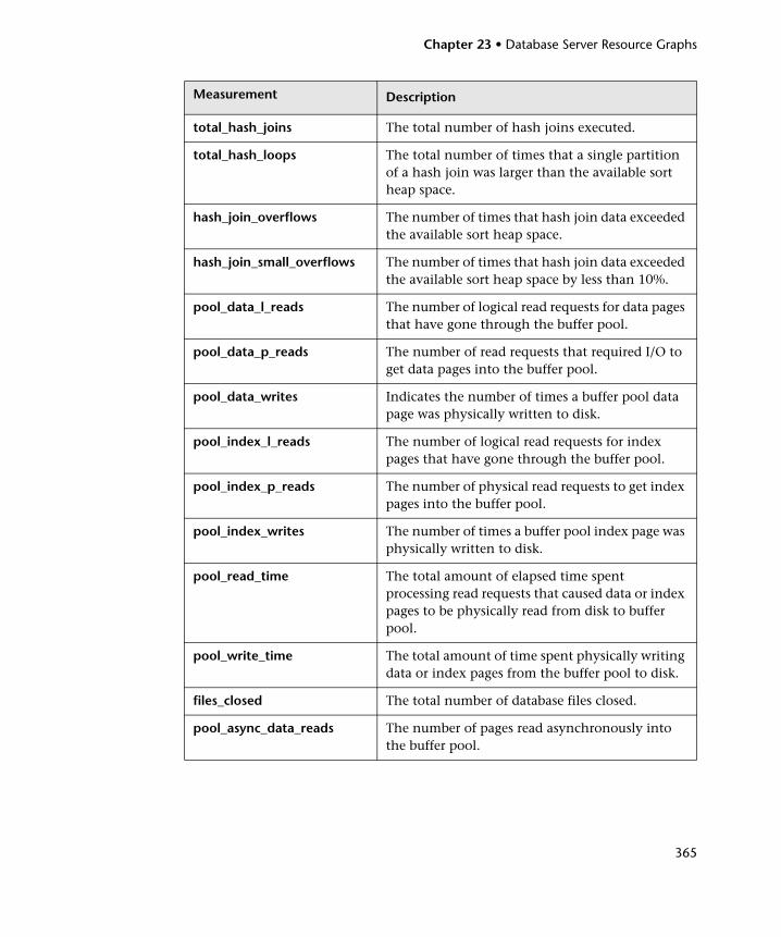
Chapter 23 • Database Server Resource Graphs
365
total_hash_joins The total number of hash joins executed.
total_hash_loops The total number of times that a single partition of a hash join was larger than the available sort heap space.
hash_join_overflows The number of times that hash join data exceeded the available sort heap space.
hash_join_small_overflows The number of times that hash join data exceeded the available sort heap space by less than 10%.
pool_data_l_reads The number of logical read requests for data pages that have gone through the buffer pool.
pool_data_p_reads The number of read requests that required I/O to get data pages into the buffer pool.
pool_data_writes Indicates the number of times a buffer pool data page was physically written to disk.
pool_index_l_reads The number of logical read requests for index pages that have gone through the buffer pool.
pool_index_p_reads The number of physical read requests to get index pages into the buffer pool.
pool_index_writes The number of times a buffer pool index page was physically written to disk.
pool_read_time The total amount of elapsed time spent processing read requests that caused data or index pages to be physically read from disk to buffer pool.
pool_write_time The total amount of time spent physically writing data or index pages from the buffer pool to disk.
files_closed The total number of database files closed.
pool_async_data_reads The number of pages read asynchronously into the buffer pool.
Measurement Description

Chapter 23 • Database Server Resource Graphs
366
pool_async_data_writes The number of times a buffer pool data page was physically written to disk by either an asynchronous page cleaner, or a pre-fetcher. A pre-fetcher may have written dirty pages to disk to make space for the pages being pre-fetched.
pool_async_index_writes The number of times a buffer pool index page was physically written to disk by either an asynchronous page cleaner, or a pre-fetcher. A pre-fetcher may have written dirty pages to disk to make space for the pages being pre-fetched.
pool_async_index_reads The number of index pages read asynchronously into the buffer pool by a pre-fetcher.
pool_async_read_time The total elapsed time spent reading by database manager pre-fetchers.
pool_async_write_time The total elapsed time spent writing data or index pages from the buffer pool to disk by database manager page cleaners.
pool_async_data_read_reqs The number of asynchronous read requests.
pool_lsn_gap_clns The number of times a page cleaner was invoked because the logging space used had reached a pre-defined criterion for the database.
pool_drty_pg_steal_clns The number of times a page cleaner was invoked because a synchronous write was needed during the victim buffer replacement for the database.
pool_drty_pg_thrsh_clns The number of times a page cleaner was invoked because a buffer pool had reached the dirty page threshold criterion for the database.
prefetch_wait_time The time an application spent waiting for an I/O server (pre-fetcher) to finish loading pages into the buffer pool.
pool_data_to_estore The number of buffer pool data pages copied to extended storage.
Measurement Description
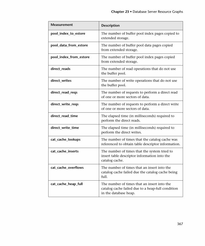
Chapter 23 • Database Server Resource Graphs
367
pool_index_to_estore The number of buffer pool index pages copied to extended storage.
pool_data_from_estore The number of buffer pool data pages copied from extended storage.
pool_index_from_estore The number of buffer pool index pages copied from extended storage.
direct_reads The number of read operations that do not use the buffer pool.
direct_writes The number of write operations that do not use the buffer pool.
direct_read_reqs The number of requests to perform a direct read of one or more sectors of data.
direct_write_reqs The number of requests to perform a direct write of one or more sectors of data.
direct_read_time The elapsed time (in milliseconds) required to perform the direct reads.
direct_write_time The elapsed time (in milliseconds) required to perform the direct writes.
cat_cache_lookups The number of times that the catalog cache was referenced to obtain table descriptor information.
cat_cache_inserts The number of times that the system tried to insert table descriptor information into the catalog cache.
cat_cache_overflows The number of times that an insert into the catalog cache failed due the catalog cache being full.
cat_cache_heap_full The number of times that an insert into the catalog cache failed due to a heap-full condition in the database heap.
Measurement Description
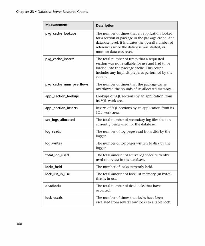
Chapter 23 • Database Server Resource Graphs
368
pkg_cache_lookups The number of times that an application looked for a section or package in the package cache. At a database level, it indicates the overall number of references since the database was started, or monitor data was reset.
pkg_cache_inserts The total number of times that a requested section was not available for use and had to be loaded into the package cache. This count includes any implicit prepares performed by the system.
pkg_cache_num_overflows The number of times that the package cache overflowed the bounds of its allocated memory.
appl_section_lookups Lookups of SQL sections by an application from its SQL work area.
appl_section_inserts Inserts of SQL sections by an application from its SQL work area.
sec_logs_allocated The total number of secondary log files that are currently being used for the database.
log_reads The number of log pages read from disk by the logger.
log_writes The number of log pages written to disk by the logger.
total_log_used The total amount of active log space currently used (in bytes) in the database.
locks_held The number of locks currently held.
lock_list_in_use The total amount of lock list memory (in bytes) that is in use.
deadlocks The total number of deadlocks that have occurred.
lock_escals The number of times that locks have been escalated from several row locks to a table lock.
Measurement Description
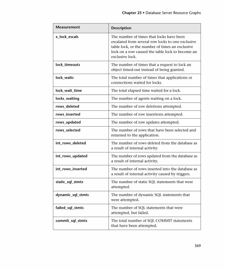
Chapter 23 • Database Server Resource Graphs
369
x_lock_escals The number of times that locks have been escalated from several row locks to one exclusive table lock, or the number of times an exclusive lock on a row caused the table lock to become an exclusive lock.
lock_timeouts The number of times that a request to lock an object timed-out instead of being granted.
lock_waits The total number of times that applications or connections waited for locks.
lock_wait_time The total elapsed time waited for a lock.
locks_waiting The number of agents waiting on a lock.
rows_deleted The number of row deletions attempted.
rows_inserted The number of row insertions attempted.
rows_updated The number of row updates attempted.
rows_selected The number of rows that have been selected and returned to the application.
int_rows_deleted The number of rows deleted from the database as a result of internal activity.
int_rows_updated The number of rows updated from the database as a result of internal activity.
int_rows_inserted The number of rows inserted into the database as a result of internal activity caused by triggers.
static_sql_stmts The number of static SQL statements that were attempted.
dynamic_sql_stmts The number of dynamic SQL statements that were attempted.
failed_sql_stmts The number of SQL statements that were attempted, but failed.
commit_sql_stmts The total number of SQL COMMIT statements that have been attempted.
Measurement Description
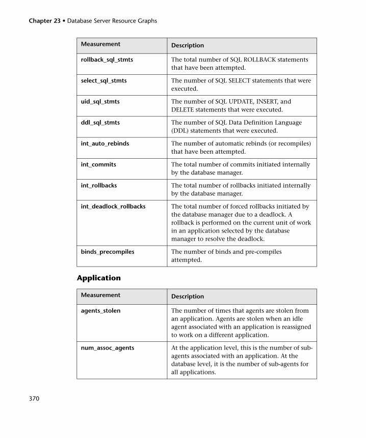
Chapter 23 • Database Server Resource Graphs
370
Application
rollback_sql_stmts The total number of SQL ROLLBACK statements that have been attempted.
select_sql_stmts The number of SQL SELECT statements that were executed.
uid_sql_stmts The number of SQL UPDATE, INSERT, and DELETE statements that were executed.
ddl_sql_stmts The number of SQL Data Definition Language (DDL) statements that were executed.
int_auto_rebinds The number of automatic rebinds (or recompiles) that have been attempted.
int_commits The total number of commits initiated internally by the database manager.
int_rollbacks The total number of rollbacks initiated internally by the database manager.
int_deadlock_rollbacks The total number of forced rollbacks initiated by the database manager due to a deadlock. A rollback is performed on the current unit of work in an application selected by the database manager to resolve the deadlock.
binds_precompiles The number of binds and pre-compiles attempted.
Measurement Description
agents_stolen The number of times that agents are stolen from an application. Agents are stolen when an idle agent associated with an application is reassigned to work on a different application.
num_assoc_agents At the application level, this is the number of sub-agents associated with an application. At the database level, it is the number of sub-agents for all applications.
Measurement Description
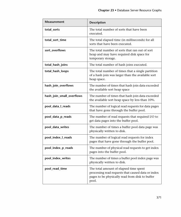
Chapter 23 • Database Server Resource Graphs
371
total_sorts The total number of sorts that have been executed.
total_sort_time The total elapsed time (in milliseconds) for all sorts that have been executed.
sort_overflows The total number of sorts that ran out of sort heap and may have required disk space for temporary storage.
total_hash_joins The total number of hash joins executed.
total_hash_loops The total number of times that a single partition of a hash join was larger than the available sort heap space.
hash_join_overflows The number of times that hash join data exceeded the available sort heap space
hash_join_small_overflows The number of times that hash join data exceeded the available sort heap space by less than 10%.
pool_data_l_reads The number of logical read requests for data pages that have gone through the buffer pool.
pool_data_p_reads The number of read requests that required I/O to get data pages into the buffer pool.
pool_data_writes The number of times a buffer pool data page was physically written to disk.
pool_index_l_reads The number of logical read requests for index pages that have gone through the buffer pool.
pool_index_p_reads The number of physical read requests to get index pages into the buffer pool.
pool_index_writes The number of times a buffer pool index page was physically written to disk.
pool_read_time The total amount of elapsed time spent processing read requests that caused data or index pages to be physically read from disk to buffer pool.
Measurement Description
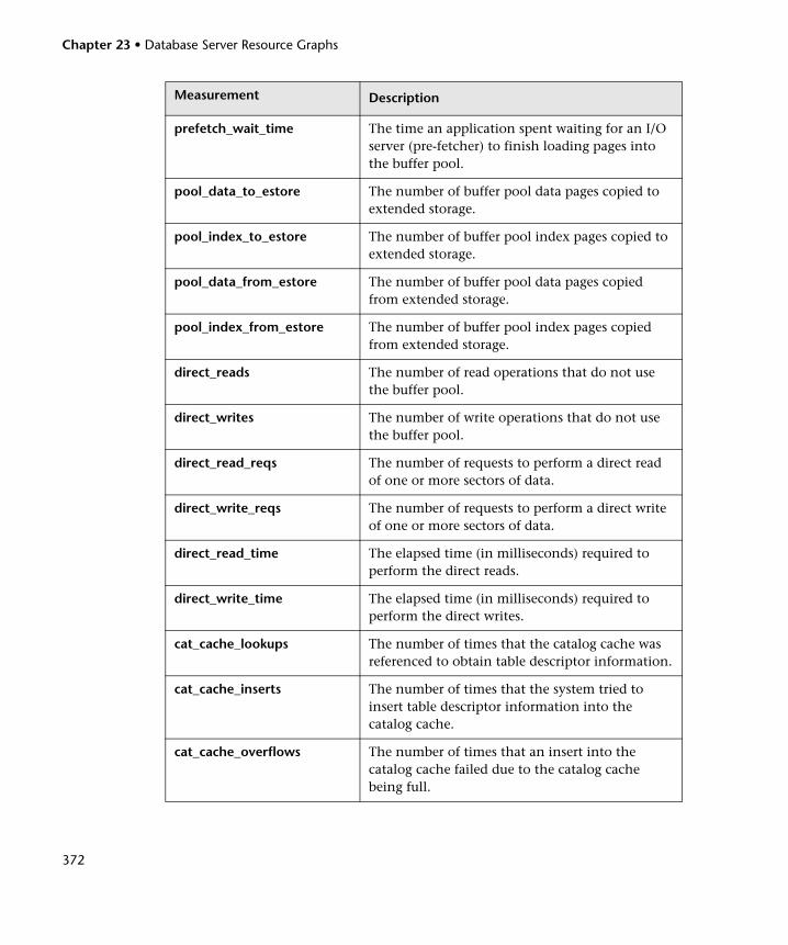
Chapter 23 • Database Server Resource Graphs
372
prefetch_wait_time The time an application spent waiting for an I/O server (pre-fetcher) to finish loading pages into the buffer pool.
pool_data_to_estore The number of buffer pool data pages copied to extended storage.
pool_index_to_estore The number of buffer pool index pages copied to extended storage.
pool_data_from_estore The number of buffer pool data pages copied from extended storage.
pool_index_from_estore The number of buffer pool index pages copied from extended storage.
direct_reads The number of read operations that do not use the buffer pool.
direct_writes The number of write operations that do not use the buffer pool.
direct_read_reqs The number of requests to perform a direct read of one or more sectors of data.
direct_write_reqs The number of requests to perform a direct write of one or more sectors of data.
direct_read_time The elapsed time (in milliseconds) required to perform the direct reads.
direct_write_time The elapsed time (in milliseconds) required to perform the direct writes.
cat_cache_lookups The number of times that the catalog cache was referenced to obtain table descriptor information.
cat_cache_inserts The number of times that the system tried to insert table descriptor information into the catalog cache.
cat_cache_overflows The number of times that an insert into the catalog cache failed due to the catalog cache being full.
Measurement Description
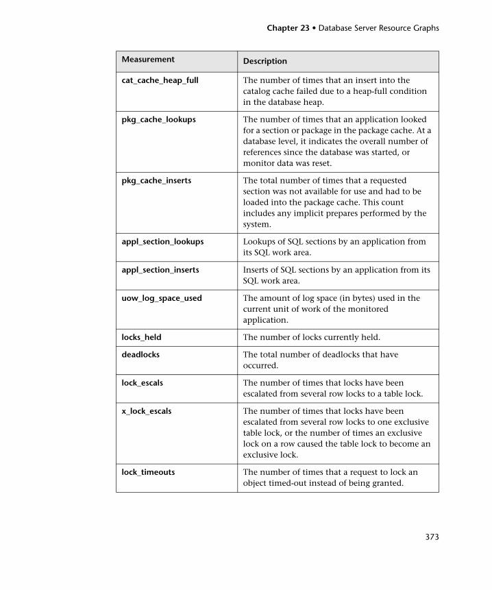
Chapter 23 • Database Server Resource Graphs
373
cat_cache_heap_full The number of times that an insert into the catalog cache failed due to a heap-full condition in the database heap.
pkg_cache_lookups The number of times that an application looked for a section or package in the package cache. At a database level, it indicates the overall number of references since the database was started, or monitor data was reset.
pkg_cache_inserts The total number of times that a requested section was not available for use and had to be loaded into the package cache. This count includes any implicit prepares performed by the system.
appl_section_lookups Lookups of SQL sections by an application from its SQL work area.
appl_section_inserts Inserts of SQL sections by an application from its SQL work area.
uow_log_space_used The amount of log space (in bytes) used in the current unit of work of the monitored application.
locks_held The number of locks currently held.
deadlocks The total number of deadlocks that have occurred.
lock_escals The number of times that locks have been escalated from several row locks to a table lock.
x_lock_escals The number of times that locks have been escalated from several row locks to one exclusive table lock, or the number of times an exclusive lock on a row caused the table lock to become an exclusive lock.
lock_timeouts The number of times that a request to lock an object timed-out instead of being granted.
Measurement Description
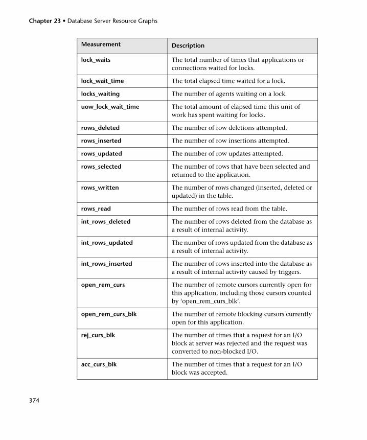
Chapter 23 • Database Server Resource Graphs
374
lock_waits The total number of times that applications or connections waited for locks.
lock_wait_time The total elapsed time waited for a lock.
locks_waiting The number of agents waiting on a lock.
uow_lock_wait_time The total amount of elapsed time this unit of work has spent waiting for locks.
rows_deleted The number of row deletions attempted.
rows_inserted The number of row insertions attempted.
rows_updated The number of row updates attempted.
rows_selected The number of rows that have been selected and returned to the application.
rows_written The number of rows changed (inserted, deleted or updated) in the table.
rows_read The number of rows read from the table.
int_rows_deleted The number of rows deleted from the database as a result of internal activity.
int_rows_updated The number of rows updated from the database as a result of internal activity.
int_rows_inserted The number of rows inserted into the database as a result of internal activity caused by triggers.
open_rem_curs The number of remote cursors currently open for this application, including those cursors counted by ‘open_rem_curs_blk’.
open_rem_curs_blk The number of remote blocking cursors currently open for this application.
rej_curs_blk The number of times that a request for an I/O block at server was rejected and the request was converted to non-blocked I/O.
acc_curs_blk The number of times that a request for an I/O block was accepted.
Measurement Description
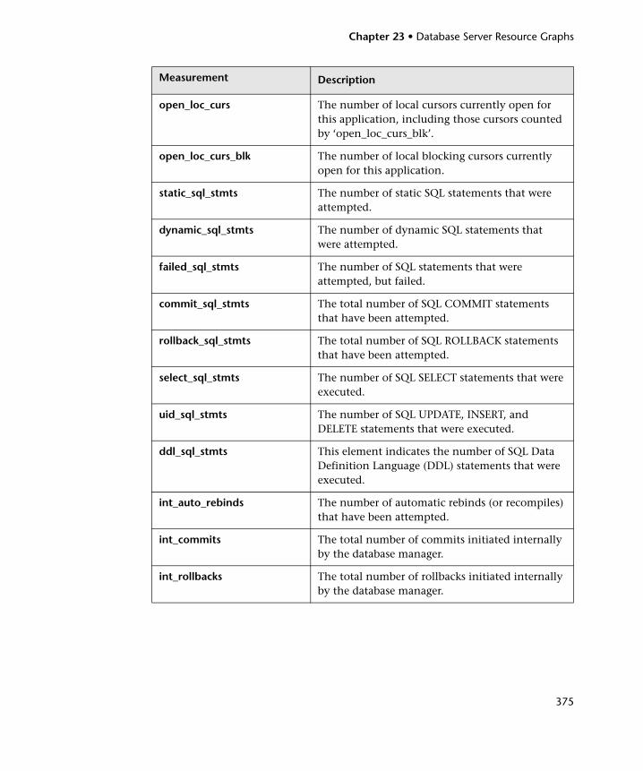
Chapter 23 • Database Server Resource Graphs
375
open_loc_curs The number of local cursors currently open for this application, including those cursors counted by ‘open_loc_curs_blk’.
open_loc_curs_blk The number of local blocking cursors currently open for this application.
static_sql_stmts The number of static SQL statements that were attempted.
dynamic_sql_stmts The number of dynamic SQL statements that were attempted.
failed_sql_stmts The number of SQL statements that were attempted, but failed.
commit_sql_stmts The total number of SQL COMMIT statements that have been attempted.
rollback_sql_stmts The total number of SQL ROLLBACK statements that have been attempted.
select_sql_stmts The number of SQL SELECT statements that were executed.
uid_sql_stmts The number of SQL UPDATE, INSERT, and DELETE statements that were executed.
ddl_sql_stmts This element indicates the number of SQL Data Definition Language (DDL) statements that were executed.
int_auto_rebinds The number of automatic rebinds (or recompiles) that have been attempted.
int_commits The total number of commits initiated internally by the database manager.
int_rollbacks The total number of rollbacks initiated internally by the database manager.
Measurement Description
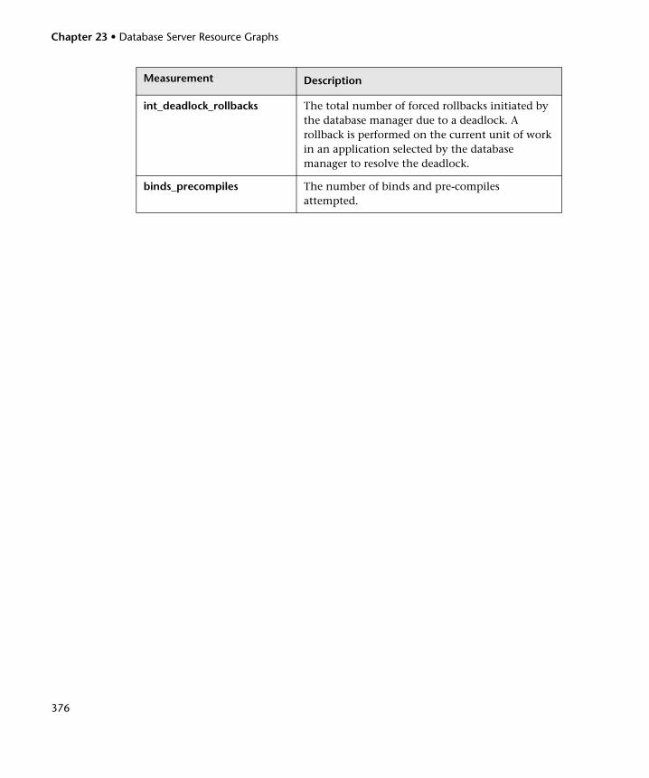
Chapter 23 • Database Server Resource Graphs
376
int_deadlock_rollbacks The total number of forced rollbacks initiated by the database manager due to a deadlock. A rollback is performed on the current unit of work in an application selected by the database manager to resolve the deadlock.
binds_precompiles The number of binds and pre-compiles attempted.
Measurement Description
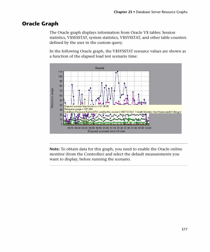
Chapter 23 • Database Server Resource Graphs
377
Oracle Graph
The Oracle graph displays information from Oracle V$ tables: Session statistics, V$SESSTAT, system statistics, V$SYSSTAT, and other table counters defined by the user in the custom query.
In the following Oracle graph, the V$SYSSTAT resource values are shown as a function of the elapsed load test scenario time:
Note: To obtain data for this graph, you need to enable the Oracle online monitor (from the Controller) and select the default measurements you want to display, before running the scenario.
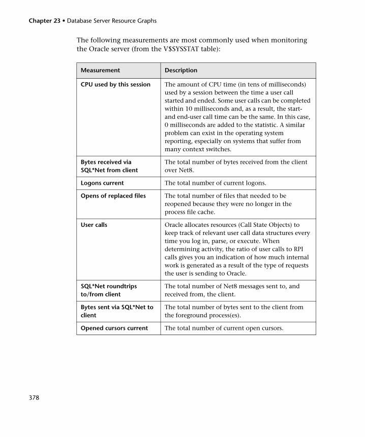
Chapter 23 • Database Server Resource Graphs
378
The following measurements are most commonly used when monitoring the Oracle server (from the V$SYSSTAT table):
Measurement Description
CPU used by this session The amount of CPU time (in tens of milliseconds) used by a session between the time a user call started and ended. Some user calls can be completed within 10 milliseconds and, as a result, the start- and end-user call time can be the same. In this case, 0 milliseconds are added to the statistic. A similar problem can exist in the operating system reporting, especially on systems that suffer from many context switches.
Bytes received via SQL*Net from client
The total number of bytes received from the client over Net8.
Logons current The total number of current logons.
Opens of replaced files The total number of files that needed to be reopened because they were no longer in the process file cache.
User calls Oracle allocates resources (Call State Objects) to keep track of relevant user call data structures every time you log in, parse, or execute. When determining activity, the ratio of user calls to RPI calls gives you an indication of how much internal work is generated as a result of the type of requests the user is sending to Oracle.
SQL*Net roundtrips to/from client
The total number of Net8 messages sent to, and received from, the client.
Bytes sent via SQL*Net to client
The total number of bytes sent to the client from the foreground process(es).
Opened cursors current The total number of current open cursors.
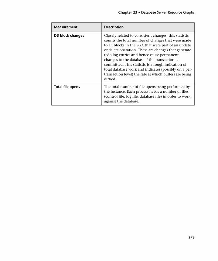
Chapter 23 • Database Server Resource Graphs
379
DB block changes Closely related to consistent changes, this statistic counts the total number of changes that were made to all blocks in the SGA that were part of an update or delete operation. These are changes that generate redo log entries and hence cause permanent changes to the database if the transaction is committed. This statistic is a rough indication of total database work and indicates (possibly on a per-transaction level) the rate at which buffers are being dirtied.
Total file opens The total number of file opens being performed by the instance. Each process needs a number of files (control file, log file, database file) in order to work against the database.
Measurement Description
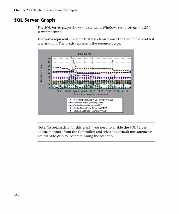
Chapter 23 • Database Server Resource Graphs
380
SQL Server Graph
The SQL Server graph shows the standard Windows resources on the SQL server machine.
The x-axis represents the time that has elapsed since the start of the load test scenario run. The y-axis represents the resource usage.
Note: To obtain data for this graph, you need to enable the SQL Server online monitor (from the Controller) and select the default measurements you want to display, before running the scenario.
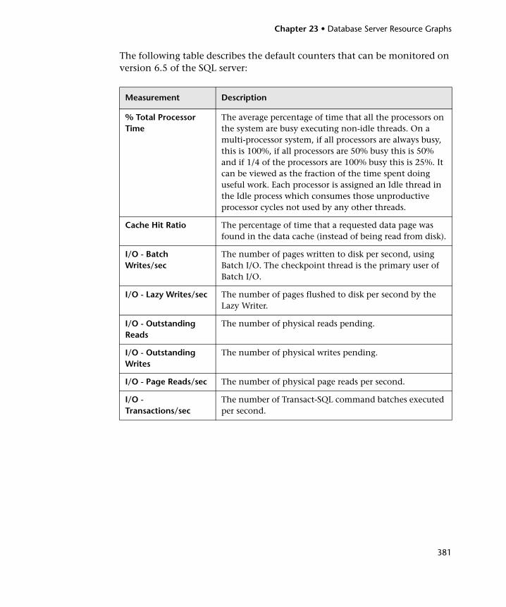
Chapter 23 • Database Server Resource Graphs
381
The following table describes the default counters that can be monitored on version 6.5 of the SQL server:
Measurement Description
% Total Processor Time
The average percentage of time that all the processors on the system are busy executing non-idle threads. On a multi-processor system, if all processors are always busy, this is 100%, if all processors are 50% busy this is 50% and if 1/4 of the processors are 100% busy this is 25%. It can be viewed as the fraction of the time spent doing useful work. Each processor is assigned an Idle thread in the Idle process which consumes those unproductive processor cycles not used by any other threads.
Cache Hit Ratio The percentage of time that a requested data page was found in the data cache (instead of being read from disk).
I/O - Batch Writes/sec
The number of pages written to disk per second, using Batch I/O. The checkpoint thread is the primary user of Batch I/O.
I/O - Lazy Writes/sec The number of pages flushed to disk per second by the Lazy Writer.
I/O - Outstanding Reads
The number of physical reads pending.
I/O - Outstanding Writes
The number of physical writes pending.
I/O - Page Reads/sec The number of physical page reads per second.
I/O - Transactions/sec
The number of Transact-SQL command batches executed per second.
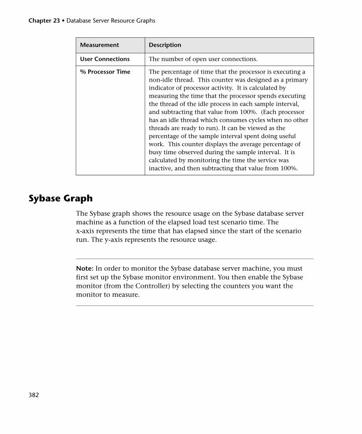
Chapter 23 • Database Server Resource Graphs
382
Sybase Graph
The Sybase graph shows the resource usage on the Sybase database server machine as a function of the elapsed load test scenario time. The x-axis represents the time that has elapsed since the start of the scenario run. The y-axis represents the resource usage.
Note: In order to monitor the Sybase database server machine, you must first set up the Sybase monitor environment. You then enable the Sybase monitor (from the Controller) by selecting the counters you want the monitor to measure.
User Connections The number of open user connections.
% Processor Time The percentage of time that the processor is executing a non-idle thread. This counter was designed as a primary indicator of processor activity. It is calculated by measuring the time that the processor spends executing the thread of the idle process in each sample interval, and subtracting that value from 100%. (Each processor has an idle thread which consumes cycles when no other threads are ready to run). It can be viewed as the percentage of the sample interval spent doing useful work. This counter displays the average percentage of busy time observed during the sample interval. It is calculated by monitoring the time the service was inactive, and then subtracting that value from 100%.
Measurement Description
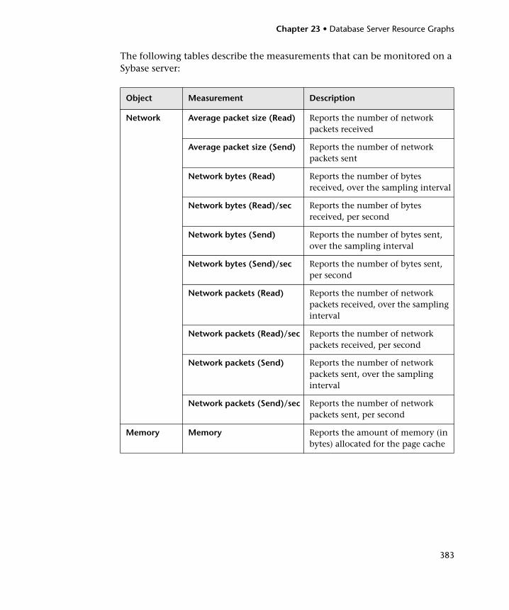
Chapter 23 • Database Server Resource Graphs
383
The following tables describe the measurements that can be monitored on a Sybase server:
Object Measurement Description
Network Average packet size (Read) Reports the number of network packets received
Average packet size (Send) Reports the number of network packets sent
Network bytes (Read) Reports the number of bytes received, over the sampling interval
Network bytes (Read)/sec Reports the number of bytes received, per second
Network bytes (Send) Reports the number of bytes sent, over the sampling interval
Network bytes (Send)/sec Reports the number of bytes sent, per second
Network packets (Read) Reports the number of network packets received, over the sampling interval
Network packets (Read)/sec Reports the number of network packets received, per second
Network packets (Send) Reports the number of network packets sent, over the sampling interval
Network packets (Send)/sec Reports the number of network packets sent, per second
Memory Memory Reports the amount of memory (in bytes) allocated for the page cache
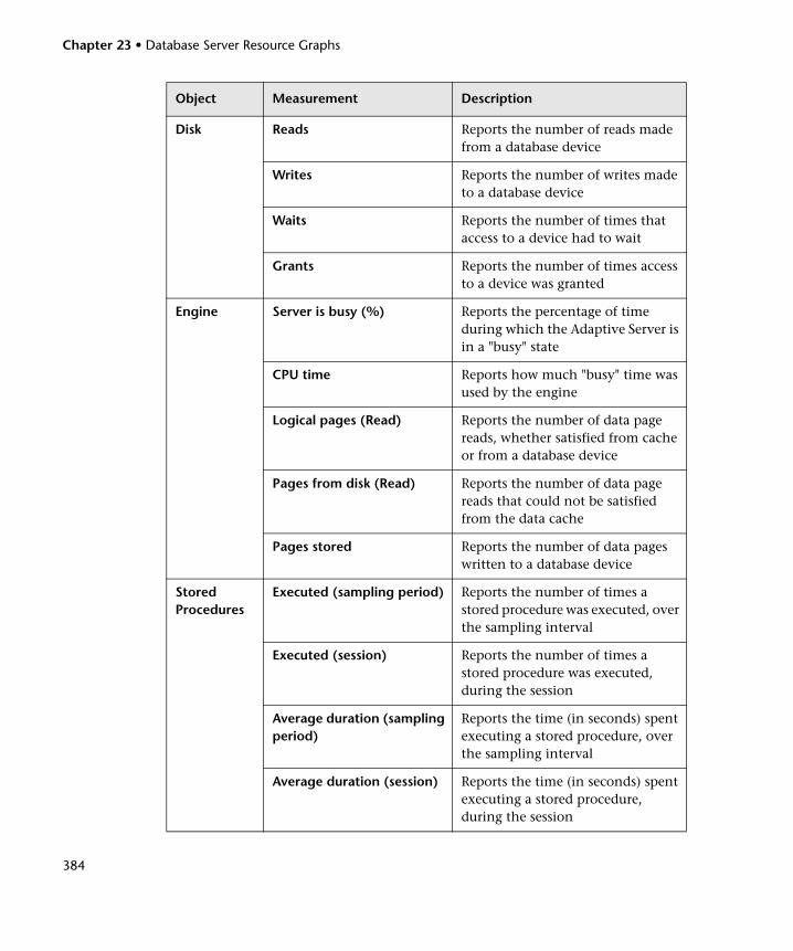
Chapter 23 • Database Server Resource Graphs
384
Disk Reads Reports the number of reads made from a database device
Writes Reports the number of writes made to a database device
Waits Reports the number of times that access to a device had to wait
Grants Reports the number of times access to a device was granted
Engine Server is busy (%) Reports the percentage of time during which the Adaptive Server is in a "busy" state
CPU time Reports how much "busy" time was used by the engine
Logical pages (Read) Reports the number of data page reads, whether satisfied from cache or from a database device
Pages from disk (Read) Reports the number of data page reads that could not be satisfied from the data cache
Pages stored Reports the number of data pages written to a database device
Stored Procedures
Executed (sampling period) Reports the number of times a stored procedure was executed, over the sampling interval
Executed (session) Reports the number of times a stored procedure was executed, during the session
Average duration (sampling period)
Reports the time (in seconds) spent executing a stored procedure, over the sampling interval
Average duration (session) Reports the time (in seconds) spent executing a stored procedure, during the session
Object Measurement Description
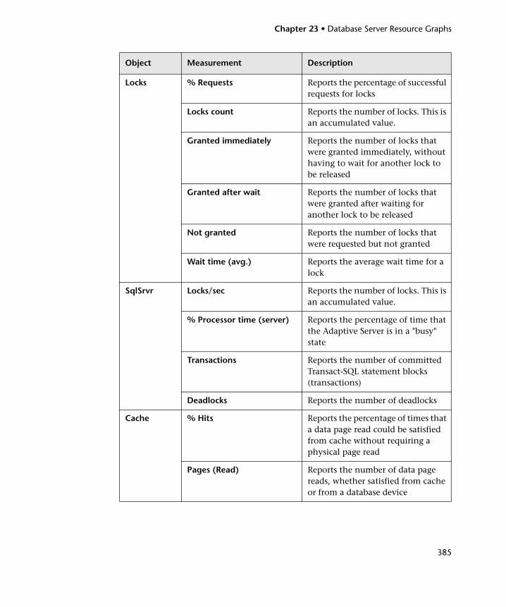
Chapter 23 • Database Server Resource Graphs
385
Locks % Requests Reports the percentage of successful requests for locks
Locks count Reports the number of locks. This is an accumulated value.
Granted immediately Reports the number of locks that were granted immediately, without having to wait for another lock to be released
Granted after wait Reports the number of locks that were granted after waiting for another lock to be released
Not granted Reports the number of locks that were requested but not granted
Wait time (avg.) Reports the average wait time for a lock
SqlSrvr Locks/sec Reports the number of locks. This is an accumulated value.
% Processor time (server) Reports the percentage of time that the Adaptive Server is in a "busy" state
Transactions Reports the number of committed Transact-SQL statement blocks (transactions)
Deadlocks Reports the number of deadlocks
Cache % Hits Reports the percentage of times that a data page read could be satisfied from cache without requiring a physical page read
Pages (Read) Reports the number of data page reads, whether satisfied from cache or from a database device
Object Measurement Description
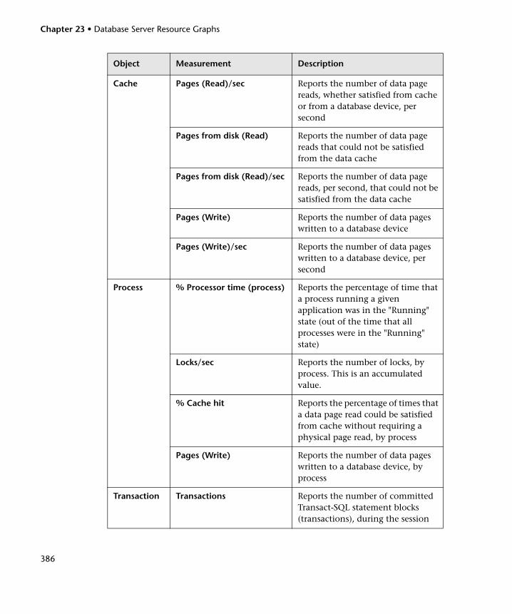
Chapter 23 • Database Server Resource Graphs
386
Cache Pages (Read)/sec Reports the number of data page reads, whether satisfied from cache or from a database device, per second
Pages from disk (Read) Reports the number of data page reads that could not be satisfied from the data cache
Pages from disk (Read)/sec Reports the number of data page reads, per second, that could not be satisfied from the data cache
Pages (Write) Reports the number of data pages written to a database device
Pages (Write)/sec Reports the number of data pages written to a database device, per second
Process % Processor time (process) Reports the percentage of time that a process running a given application was in the "Running" state (out of the time that all processes were in the "Running" state)
Locks/sec Reports the number of locks, by process. This is an accumulated value.
% Cache hit Reports the percentage of times that a data page read could be satisfied from cache without requiring a physical page read, by process
Pages (Write) Reports the number of data pages written to a database device, by process
Transaction Transactions Reports the number of committed Transact-SQL statement blocks (transactions), during the session
Object Measurement Description
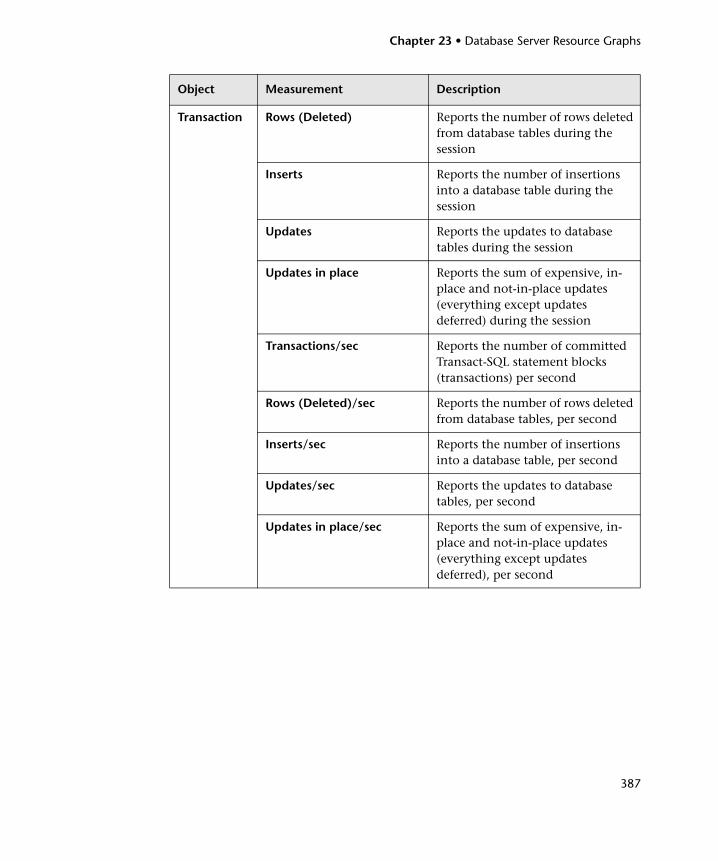
Chapter 23 • Database Server Resource Graphs
387
Transaction Rows (Deleted) Reports the number of rows deleted from database tables during the session
Inserts Reports the number of insertions into a database table during the session
Updates Reports the updates to database tables during the session
Updates in place Reports the sum of expensive, in-place and not-in-place updates (everything except updates deferred) during the session
Transactions/sec Reports the number of committed Transact-SQL statement blocks (transactions) per second
Rows (Deleted)/sec Reports the number of rows deleted from database tables, per second
Inserts/sec Reports the number of insertions into a database table, per second
Updates/sec Reports the updates to database tables, per second
Updates in place/sec Reports the sum of expensive, in-place and not-in-place updates (everything except updates deferred), per second
Object Measurement Description

Chapter 23 • Database Server Resource Graphs
388
389
24 Streaming Media Graphs
After a load test scenario run, you can use the Streaming Media graphs to analyze RealPlayer Client, RealPlayer Server, and Windows Media Server performance.
This chapter includes:
➤ About Streaming Media Graphs on page 389
➤ Real Client Graph on page 391
➤ Real Server Graph on page 393
➤ Windows Media Server Graph on page 394
➤ Media Player Client Graph on page 396
About Streaming Media Graphs
Streaming Media Resource graphs provide you with performance information for the RealPlayer Client, RealPlayer Server, Windows Media Server, and Media Player Client machines.
In order to obtain data for Streaming Media Resource graphs, you need to install the RealPlayer Client and activate the online monitor for the RealPlayer Server or Windows Media Server before running the load test scenario.
When you set up the online monitor for the RealPlayer Server or Windows Media Server, you indicate which statistics and measurements to monitor. For more information on installing and configuring the Streaming Media Resource monitors, refer to the HP LoadRunner Controller User Guide.
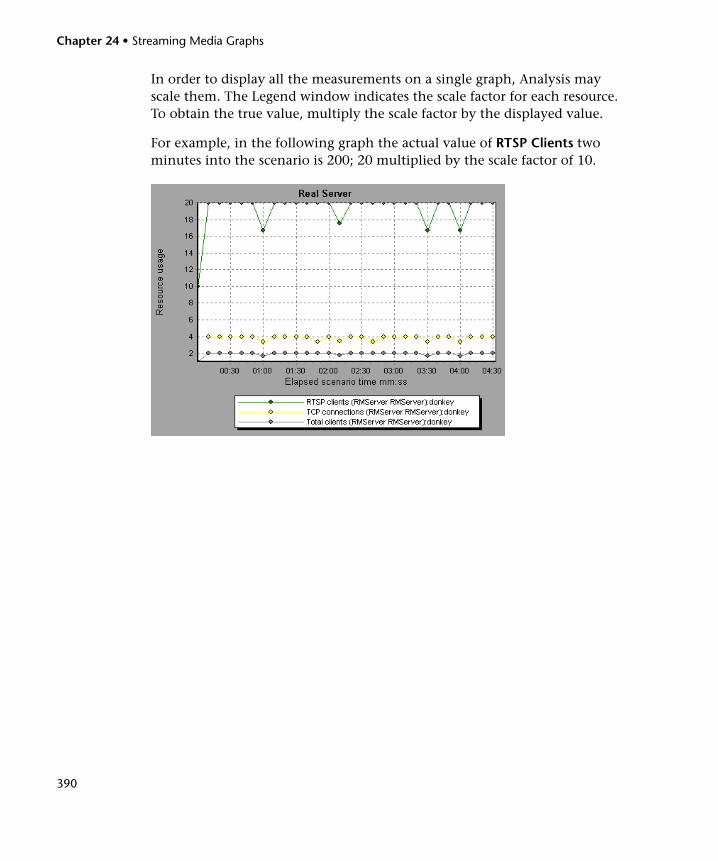
Chapter 24 • Streaming Media Graphs
390
In order to display all the measurements on a single graph, Analysis may scale them. The Legend window indicates the scale factor for each resource. To obtain the true value, multiply the scale factor by the displayed value.
For example, in the following graph the actual value of RTSP Clients two minutes into the scenario is 200; 20 multiplied by the scale factor of 10.
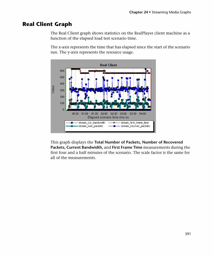
Chapter 24 • Streaming Media Graphs
391
Real Client Graph
The Real Client graph shows statistics on the RealPlayer client machine as a function of the elapsed load test scenario time.
The x-axis represents the time that has elapsed since the start of the scenario run. The y-axis represents the resource usage.
This graph displays the Total Number of Packets, Number of Recovered Packets, Current Bandwidth, and First Frame Time measurements during the first four and a half minutes of the scenario. The scale factor is the same for all of the measurements.
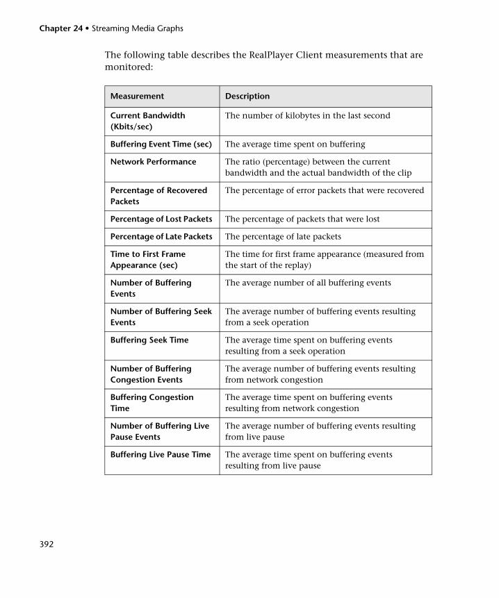
Chapter 24 • Streaming Media Graphs
392
The following table describes the RealPlayer Client measurements that are monitored:
Measurement Description
Current Bandwidth (Kbits/sec)
The number of kilobytes in the last second
Buffering Event Time (sec) The average time spent on buffering
Network Performance The ratio (percentage) between the current bandwidth and the actual bandwidth of the clip
Percentage of Recovered Packets
The percentage of error packets that were recovered
Percentage of Lost Packets The percentage of packets that were lost
Percentage of Late Packets The percentage of late packets
Time to First Frame Appearance (sec)
The time for first frame appearance (measured from the start of the replay)
Number of Buffering Events
The average number of all buffering events
Number of Buffering Seek Events
The average number of buffering events resulting from a seek operation
Buffering Seek Time The average time spent on buffering events resulting from a seek operation
Number of Buffering Congestion Events
The average number of buffering events resulting from network congestion
Buffering Congestion Time
The average time spent on buffering events resulting from network congestion
Number of Buffering Live Pause Events
The average number of buffering events resulting from live pause
Buffering Live Pause Time The average time spent on buffering events resulting from live pause
Chapter 24 • Streaming Media Graphs
393
Real Server Graph
The Real Server graph shows RealPlayer server statistics as a function of the elapsed load test scenario time.
The x-axis represents the time that has elapsed since the start of the scenario run. The y-axis represents the resource usage.
In this graph, the number of RTSP Clients remained steady during the first four and a half minutes of the scenario. The Total Bandwidth and number of Total Clients fluctuated slightly. The number of TCP Connections fluctuated more significantly.
The scale factor for the TCP Connections and Total Clients measurements is 10, and the scale factor for Total Bandwidth is 1/1000.
Note: To obtain data for this graph, you need to enable the RealPlayer Server online monitor (from the Controller) and select the default measurements you want to display, before running the scenario.
Chapter 24 • Streaming Media Graphs
394
The following default measurements are available for the RealPlayer Server:
Windows Media Server Graph
The Windows Media Server graph shows the Windows Media server statistics as a function of the elapsed load test scenario time. The x-axis represents the time that has elapsed since the start of the scenario run. The y-axis represents the resource usage.
Note: To obtain data for this graph, you need to enable the Windows Media Server online monitor (from the Controller) and select the default measurements you want to display, before running the scenario.
Measurement Description
Encoder Connections The number of active encoder connections
HTTP Clients The number of active clients using HTTP
Monitor Connections The number of active server monitor connections
Multicast Connections The number of active multicast connections
PNA Clients The number of active clients using PNA
RTSP Clients The number of active clients using RTSP
Splitter Connections The number of active splitter connections
TCP Connections The number of active TCP connections
Total Bandwidth The number of bits per second being consumed
Total Clients The total number of active clients
UDP Clients The number of active UDP connections
Chapter 24 • Streaming Media Graphs
395
The following default measurements are available for the Windows Media Server:
Measurement Description
Active Live Unicast Streams (Windows)
The number of live unicast streams that are being streamed.
Active Streams The number of streams that are being streamed.
Active TCP Streams The number of TCP streams that are being streamed.
Active UDP Streams The number of UDP streams that are being streamed.
Aggregate Read Rate The total, aggregate rate (bytes/sec) of file reads.
Aggregate Send Rate The total, aggregate rate (bytes/sec) of stream transmission.
Connected Clients The number of clients connected to the server.
Connection Rate The rate at which clients are connecting to the server.
Controllers The number of controllers currently connected to the server.
HTTP Streams The number of HTTP streams being streamed.
Late Reads The number of late read completions per second.
Pending Connections The number of clients that are attempting to connect to the server, but are not yet connected. This number may be high if the server is running near maximum capacity and cannot process a large number of connection requests in a timely manner.
Stations The number of station objects that currently exist on the server.
Streams The number of stream objects that currently exist on the server.
Stream Errors The cumulative number of errors occurring per second.
Chapter 24 • Streaming Media Graphs
396
Media Player Client Graph
The Media Player Client graph shows statistics on the Windows Media Player client machine as a function of the elapsed load test scenario time.
The x-axis represents the time that has elapsed since the start of the scenario run. The y-axis represents the resource usage.
In this graph, the Total number of recovered packets remained steady during the first two and a half minutes of the scenario. The Number of Packets and Stream Interruptions fluctuated significantly. The Average Buffering Time increased moderately, and the Player Bandwidth increased and then decreased moderately.
The scale factor for the Stream Interruptions and Average Buffering Events measurements is 10, and the scale factor for Player Bandwidth is 1/10.
Chapter 24 • Streaming Media Graphs
397
The following table describes the Media Player Client measurements that are monitored:
Measurement Description
Average Buffering Events The number of times Media Player Client had to buffer incoming media data due to insufficient media content
Average Buffering Time (sec)
The time spent by Media Player Client waiting for sufficient amount of media data in order to continue playing media clip
Current bandwidth (Kbits/sec)
The number of kbits per second received
Number of Packets The number of packets sent by server for a particular media clip
Stream Interruptions The number of interruptions encountered by Media Player Client while playing a media clip. This measurement includes the number of times Media Player Client had to buffer incoming media data, and any errors that occurred during playback.
Stream Quality (Packet-level)
The percentage ratio of packets received to total packets
Stream Quality (Sampling-level)
The percentage of stream samples received on time (no delays in reception)
Total number of recovered packets
The number of lost packets that were recovered. This value is only relevant during network playback.
Total number of lost packets
The number of lost packets that were not recovered. This value is only relevant during network playback.

Chapter 24 • Streaming Media Graphs
398
399
25 ERP/CRM Server Resource Graphs
After a load test scenario run, you can use the ERP/CRM server resource monitor graphs to analyze ERP/CRM server resource performance.
This chapter includes:
➤ About ERP/CRM Server Resource Graphs on page 400
➤ SAP Graph on page 400
➤ SAPGUI Graph on page 403
➤ SAP Portal Graph on page 406
➤ SAP CCMS Graph on page 408
➤ Siebel Server Manager Graph on page 409
➤ Siebel Web Server Graph on page 412
➤ PeopleSoft (Tuxedo) Graph on page 414
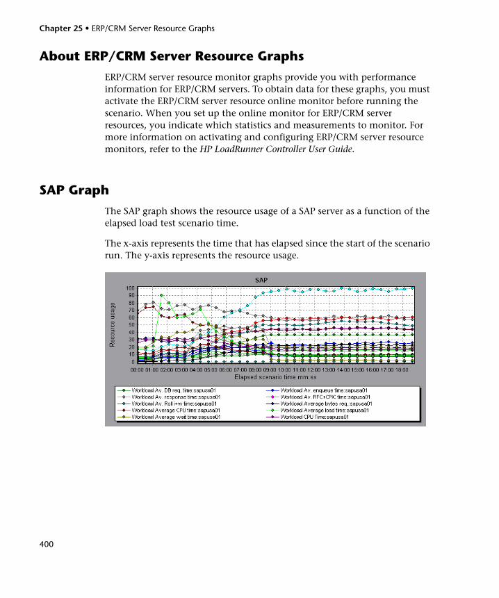
Chapter 25 • ERP/CRM Server Resource Graphs
400
About ERP/CRM Server Resource Graphs
ERP/CRM server resource monitor graphs provide you with performance information for ERP/CRM servers. To obtain data for these graphs, you must activate the ERP/CRM server resource online monitor before running the scenario. When you set up the online monitor for ERP/CRM server resources, you indicate which statistics and measurements to monitor. For more information on activating and configuring ERP/CRM server resource monitors, refer to the HP LoadRunner Controller User Guide.
SAP Graph
The SAP graph shows the resource usage of a SAP server as a function of the elapsed load test scenario time.
The x-axis represents the time that has elapsed since the start of the scenario run. The y-axis represents the resource usage.
Chapter 25 • ERP/CRM Server Resource Graphs
401
Note: To obtain data for this graph, you need to enable the SAP online monitor (from the Controller) and select the default measurements you want to display, before running the scenario.
There are differences in the scale factor for some of the measurements.
The following are the most commonly monitored counters for a SAP server:
Measurement Description
Average CPU time The average CPU time used in the work process.
Average response time The average response time, measured from the time a dialog sends a request to the dispatcher work process, through the processing of the dialog, until the dialog is completed and the data is passed to the presentation layer. The response time between the SAP GUI and the dispatcher is not included in this value.
Average wait time The average amount of time that an unprocessed dialog step waits in the dispatcher queue for a free work process. Under normal conditions, the dispatcher work process should pass a dialog step to the application process immediately after receiving the request from the dialog step. Under these conditions, the average wait time would be a few milliseconds. A heavy load on the application server or on the entire system causes queues at the dispatcher queue.
Average load time The time needed to load and generate objects, such as ABAP source code and screen information, from the database.
Database calls The number of parsed requests sent to the database.
Chapter 25 • ERP/CRM Server Resource Graphs
402
Database requests The number of logical ABAP requests for data in the database. These requests are passed through the R/3 database interface and parsed into individual database calls. The proportion of database calls to database requests is important. If access to information in a table is buffered in the SAP buffers, database calls to the database server are not required. Therefore, the ratio of calls/requests gives an overall indication of the efficiency of table buffering. A good ratio would be 1:10.
Roll ins The number of rolled-in user contexts.
Roll outs The number of rolled-out user contexts.
Roll in time The processing time for roll ins.
Roll out time The processing time for roll outs.
Roll wait time The queue time in the roll area. When synchronous RFCs are called, the work process executes a roll out and may have to wait for the end of the RFC in the roll area, even if the dialog step is not yet completed. In the roll area, RFC server programs can also wait for other RFCs sent to them.
Average time per logical DB call
The average response time for all commands sent to the database system (in milliseconds). The time depends on the CPU capacity of the database server, the network, the buffering, and on the input/output capabilities of the database server. Access times for buffered tables are many magnitudes faster and are not considered in the measurement.
Measurement Description
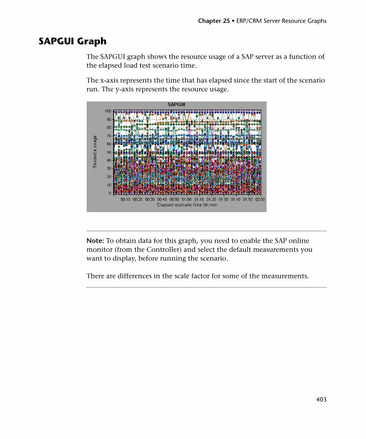
Chapter 25 • ERP/CRM Server Resource Graphs
403
SAPGUI Graph
The SAPGUI graph shows the resource usage of a SAP server as a function of the elapsed load test scenario time.
The x-axis represents the time that has elapsed since the start of the scenario run. The y-axis represents the resource usage.
Note: To obtain data for this graph, you need to enable the SAP online monitor (from the Controller) and select the default measurements you want to display, before running the scenario.
There are differences in the scale factor for some of the measurements.
Chapter 25 • ERP/CRM Server Resource Graphs
404
The following are the most commonly monitored counters:
Measurement Description
Average CPU time The average CPU time used in the work process.
Average response time The average response time, measured from the time a dialog sends a request to the dispatcher work process, through the processing of the dialog, until the dialog is completed and the data is passed to the presentation layer. The response time between the SAPGUI and the dispatcher is not included in this value.
Average wait time The average amount of time that an unprocessed dialog step waits in the dispatcher queue for a free work process. Under normal conditions, the dispatcher work process should pass a dialog step to the application process immediately after receiving the request from the dialog step. Under these conditions, the average wait time would be a few milliseconds. A heavy load on the application server or on the entire system causes queues at the dispatcher queue.
Average load time The time needed to load and generate objects, such as ABAP source code and screen information, from the database.
Database calls The number of parsed requests sent to the database.
Database requests The number of logical ABAP requests for data in the database. These requests are passed through the R/3 database interface and parsed into individual database calls. The proportion of database calls to database requests is important. If access to information in a table is buffered in the SAP buffers, database calls to the database server are not required. Therefore, the ratio of calls/requests gives an overall indication of the efficiency of table buffering. A good ratio would be 1:10.
Roll ins The number of rolled-in user contexts.
Chapter 25 • ERP/CRM Server Resource Graphs
405
Roll outs The number of rolled-out user contexts.
Roll in time The processing time for roll ins.
Roll out time The processing time for roll outs.
Roll wait time The queue time in the roll area. When synchronous RFCs are called, the work process executes a roll out and may have to wait for the end of the RFC in the roll area, even if the dialog step is not yet completed. In the roll area, RFC server programs can also wait for other RFCs sent to them.
Average time per logical DB call
The average response time for all commands sent to the database system (in milliseconds). The time depends on the CPU capacity of the database server, the network, the buffering, and on the input/output capabilities of the database server. Access times for buffered tables are many magnitudes faster and are not considered in the measurement.
Measurement Description

Chapter 25 • ERP/CRM Server Resource Graphs
406
SAP Portal Graph
The SAP Portal graph shows the resource usage of your SAP Portal server as a function of the elapsed load test scenario time.
Note: To obtain data for this graph, you need to enable the SAP Portal monitor (from the Controller) and select the default measurements you want to display, before running the scenario.
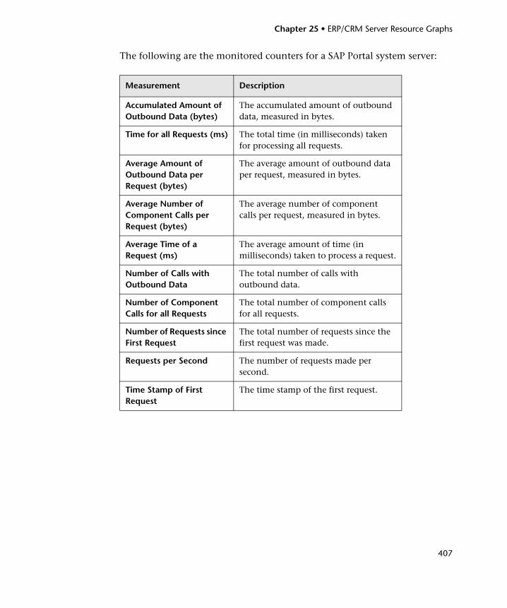
Chapter 25 • ERP/CRM Server Resource Graphs
407
The following are the monitored counters for a SAP Portal system server:
Measurement Description
Accumulated Amount of Outbound Data (bytes)
The accumulated amount of outbound data, measured in bytes.
Time for all Requests (ms) The total time (in milliseconds) taken for processing all requests.
Average Amount of Outbound Data per Request (bytes)
The average amount of outbound data per request, measured in bytes.
Average Number of Component Calls per Request (bytes)
The average number of component calls per request, measured in bytes.
Average Time of a Request (ms)
The average amount of time (in milliseconds) taken to process a request.
Number of Calls with Outbound Data
The total number of calls with outbound data.
Number of Component Calls for all Requests
The total number of component calls for all requests.
Number of Requests since First Request
The total number of requests since the first request was made.
Requests per Second The number of requests made per second.
Time Stamp of First Request
The time stamp of the first request.
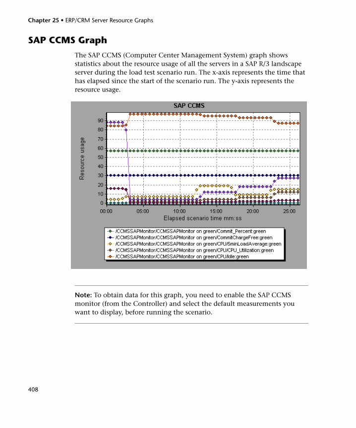
Chapter 25 • ERP/CRM Server Resource Graphs
408
SAP CCMS Graph
The SAP CCMS (Computer Center Management System) graph shows statistics about the resource usage of all the servers in a SAP R/3 landscape server during the load test scenario run. The x-axis represents the time that has elapsed since the start of the scenario run. The y-axis represents the resource usage.
Note: To obtain data for this graph, you need to enable the SAP CCMS monitor (from the Controller) and select the default measurements you want to display, before running the scenario.
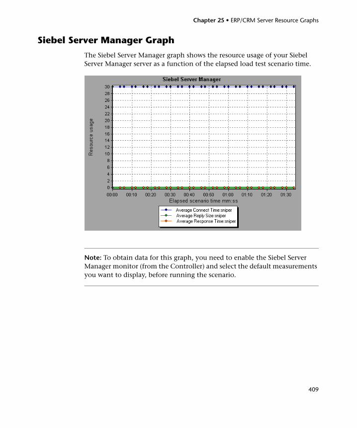
Chapter 25 • ERP/CRM Server Resource Graphs
409
Siebel Server Manager Graph
The Siebel Server Manager graph shows the resource usage of your Siebel Server Manager server as a function of the elapsed load test scenario time.
Note: To obtain data for this graph, you need to enable the Siebel Server Manager monitor (from the Controller) and select the default measurements you want to display, before running the scenario.
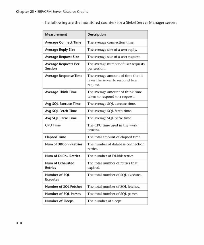
Chapter 25 • ERP/CRM Server Resource Graphs
410
The following are the monitored counters for a Siebel Server Manager server:
Measurement Description
Average Connect Time The average connection time.
Average Reply Size The average size of a user reply.
Average Request Size The average size of a user request.
Average Requests Per Session
The average number of user requests per session.
Average Response Time The average amount of time that it takes the server to respond to a request.
Average Think Time The average amount of think time taken to respond to a request.
Avg SQL Execute Time The average SQL execute time.
Avg SQL Fetch Time The average SQL fetch time.
Avg SQL Parse Time The average SQL parse time.
CPU Time The CPU time used in the work process.
Elapsed Time The total amount of elapsed time.
Num of DBConn Retries The number of database connection retries.
Num of DLRbk Retries The number of DLRbk retries.
Num of Exhausted Retries
The total number of retries that expired.
Number of SQL Executes
The total number of SQL executes.
Number of SQL Fetches The total number of SQL fetches.
Number of SQL Parses The total number of SQL parses.
Number of Sleeps The number of sleeps.
Chapter 25 • ERP/CRM Server Resource Graphs
411
Object Manager Errors The total number of object manager errors.
Reply Messages The total number of reply messages.
Request Messages The total number of request messages.
SQL Execute Time The total SQL execute time.
SQL Fetch Time The total SQL fetch time.
SQL Parse Time The total SQL parse time.
Sleep Time The total sleep time.
Tests Attempted The number of tests attempted.
Tests Failed The number of tests that failed.
Tests Successful The number of tests that were successful.
Total Reply Size The total reply size, measured in bytes.
Total Request Size The total request size, measured in bytes.
Total Response Time The total response time.
Total Tasks The total number of tasks.
Total Think Time The total think time.
Measurement Description
Chapter 25 • ERP/CRM Server Resource Graphs
412
Siebel Web Server Graph
The Siebel Web Server graph shows the resource usage of your Siebel Web Server as a function of the elapsed load test scenario time.
Note: To obtain data for this graph, you need to enable the Siebel Web Server monitor (from the Controller) and select the default measurements you want to display, before running the scenario.
Chapter 25 • ERP/CRM Server Resource Graphs
413
The following are the monitored counters for a Siebel Web Server:
Measurement Description
Anonymous sessions requested from the pool
The number of anonymous sessions requested from the pool.
Open Session Time The time taken for users to log on to the system.
Anon Session Removed The number of anonymous sessions removed from the pool.
Anon Session Available The number of anonymous sessions available in the pool.
Anonymous sessions returns to the pool
The number of anonymous sessions returned to the pool.
Response Time The time taken to respond to a user request.
Close Session Time The time taken for users to log off the system.
Request Time The time taken to process the user request.
Chapter 25 • ERP/CRM Server Resource Graphs
414
PeopleSoft (Tuxedo) Graph
The PeopleSoft (Tuxedo) graph shows the resource usage of your Tuxedo server as a function of the elapsed load test scenario time.
Note: To obtain data for this graph, you need to enable the PeopleSoft (Tuxedo) monitor (from the Controller) and select the default measurements you want to display, before running the scenario.
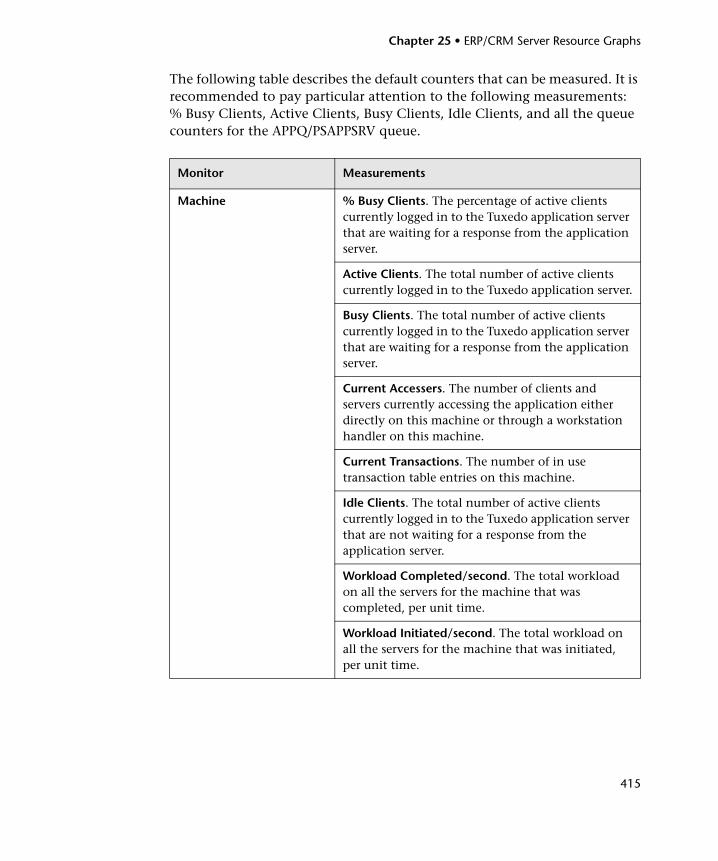
Chapter 25 • ERP/CRM Server Resource Graphs
415
The following table describes the default counters that can be measured. It is recommended to pay particular attention to the following measurements: % Busy Clients, Active Clients, Busy Clients, Idle Clients, and all the queue counters for the APPQ/PSAPPSRV queue.
Monitor Measurements
Machine % Busy Clients. The percentage of active clients currently logged in to the Tuxedo application server that are waiting for a response from the application server.
Active Clients. The total number of active clients currently logged in to the Tuxedo application server.
Busy Clients. The total number of active clients currently logged in to the Tuxedo application server that are waiting for a response from the application server.
Current Accessers. The number of clients and servers currently accessing the application either directly on this machine or through a workstation handler on this machine.
Current Transactions. The number of in use transaction table entries on this machine.
Idle Clients. The total number of active clients currently logged in to the Tuxedo application server that are not waiting for a response from the application server.
Workload Completed/second. The total workload on all the servers for the machine that was completed, per unit time.
Workload Initiated/second. The total workload on all the servers for the machine that was initiated, per unit time.
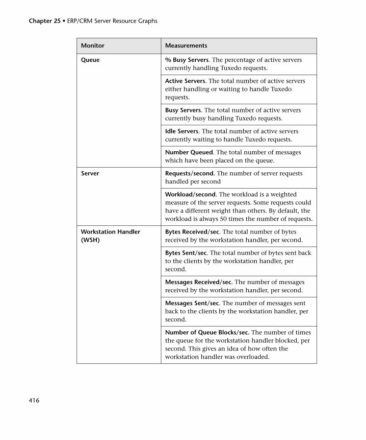
Chapter 25 • ERP/CRM Server Resource Graphs
416
Queue % Busy Servers. The percentage of active servers currently handling Tuxedo requests.
Active Servers. The total number of active servers either handling or waiting to handle Tuxedo requests.
Busy Servers. The total number of active servers currently busy handling Tuxedo requests.
Idle Servers. The total number of active servers currently waiting to handle Tuxedo requests.
Number Queued. The total number of messages which have been placed on the queue.
Server Requests/second. The number of server requests handled per second
Workload/second. The workload is a weighted measure of the server requests. Some requests could have a different weight than others. By default, the workload is always 50 times the number of requests.
Workstation Handler (WSH)
Bytes Received/sec. The total number of bytes received by the workstation handler, per second.
Bytes Sent/sec. The total number of bytes sent back to the clients by the workstation handler, per second.
Messages Received/sec. The number of messages received by the workstation handler, per second.
Messages Sent/sec. The number of messages sent back to the clients by the workstation handler, per second.
Number of Queue Blocks/sec. The number of times the queue for the workstation handler blocked, per second. This gives an idea of how often the workstation handler was overloaded.
Monitor Measurements
417
26 Java Performance Graphs
Note: Java performance graphs are available only when you are analyzing load test scenarios that were run in version 8.1 (and earlier) of the Controller.
After a scenario run, you can use the Java performance monitor graphs to analyze the performance of Java™ 2 Platform, Enterprise Edition (J2EE) objects and Java-based applications.
This chapter includes:
➤ About Java Performance Graphs on page 417
➤ J2EE Graph on page 418
About Java Performance Graphs
Java performance graphs provide you with performance information for Java™ 2 Platform, Enterprise Edition (J2EE) objects, and Java-based applications using J2EE. To obtain data for these graphs, you need to activate the Java performance monitor before running the load test scenario.
When you set up the Java performance online monitor, you indicate which statistics and measurements to monitor. For more information on activating and configuring the Java performance monitor, refer to the HP LoadRunner Controller User Guide.
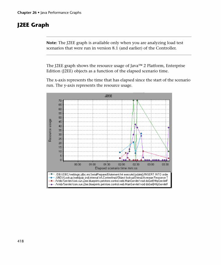
Chapter 26 • Java Performance Graphs
418
J2EE Graph
Note: The J2EE graph is available only when you are analyzing load test scenarios that were run in version 8.1 (and earlier) of the Controller.
The J2EE graph shows the resource usage of Java™ 2 Platform, Enterprise Edition (J2EE) objects as a function of the elapsed scenario time.
The x-axis represents the time that has elapsed since the start of the scenario run. The y-axis represents the resource usage.
Chapter 26 • Java Performance Graphs
419
Note: To obtain data for this graph, you must first install and activate the J2EE monitor on the application server machine. You then configure the J2EE monitor on the client machine by selecting the counters you want the monitor to measure.
The following J2EE counters are available for monitoring Servlets/JSP's, JNDI, EJB, and JDBC method calls:
Measurement Description
Average Response Time The average response time (in milliseconds) of the J2EE object being monitored.
Method Calls per Second The number of J2EE object method calls per second.

Chapter 26 • Java Performance Graphs
420
421
27 Application Component Graphs
After a load test scenario run, you can use the application component monitor graphs to analyze the performance of an application’s Microsoft COM+ interfaces and methods and Microsoft .NET CLR classes and methods.
This chapter includes:
➤ About Microsoft COM+ Performance Graphs on page 422
➤ About Microsoft .NET CLR Performance Graphs on page 422
➤ Microsoft COM+ Graph on page 423
➤ COM+ Breakdown Graph on page 427
➤ COM+ Average Response Time Graph on page 429
➤ COM+ Call Count Graph on page 431
➤ COM+ Call Count Distribution Graph on page 433
➤ COM+ Call Count Per Second Graph on page 435
➤ COM+ Total Operation Time Graph on page 437
➤ COM+ Total Operation Time Distribution Graph on page 439
➤ .NET Breakdown Graph on page 441
➤ .NET Average Response Time Graph on page 443
➤ .NET Call Count Graph on page 444
➤ .NET Call Count Distribution Graph on page 446
➤ .NET Call Count per Second Graph on page 447
➤ .NET Total Operation Time Distribution Graph on page 448
Chapter 27 • Application Component Graphs
422
➤ .NET Total Operation Time Graph on page 449
➤ .NET Resources Graph on page 450
About Microsoft COM+ Performance Graphs
Microsoft COM+ performance graphs provide you with performance information for COM+ interfaces and methods.
In order to obtain data for these graphs, you need to activate the various Microsoft COM+ performance monitors before running the load test scenario.
When you set up the Microsoft COM+ performance online monitors, you indicate which statistics and measurements to monitor. For more information on activating and configuring the Microsoft COM+ performance monitors, refer to the HP LoadRunner Controller User Guide.
About Microsoft .NET CLR Performance Graphs
The .NET CLR performance graphs provide you with performance information for .NET classes and methods. To obtain data for these graphs, you must activate the .NET CLR performance monitor before running the load test scenario run.
Displayed measurements are specified using the .NET monitor. For more information on activating and configuring the .NET CLR performance monitor, refer to the HP LoadRunner Controller User Guide.
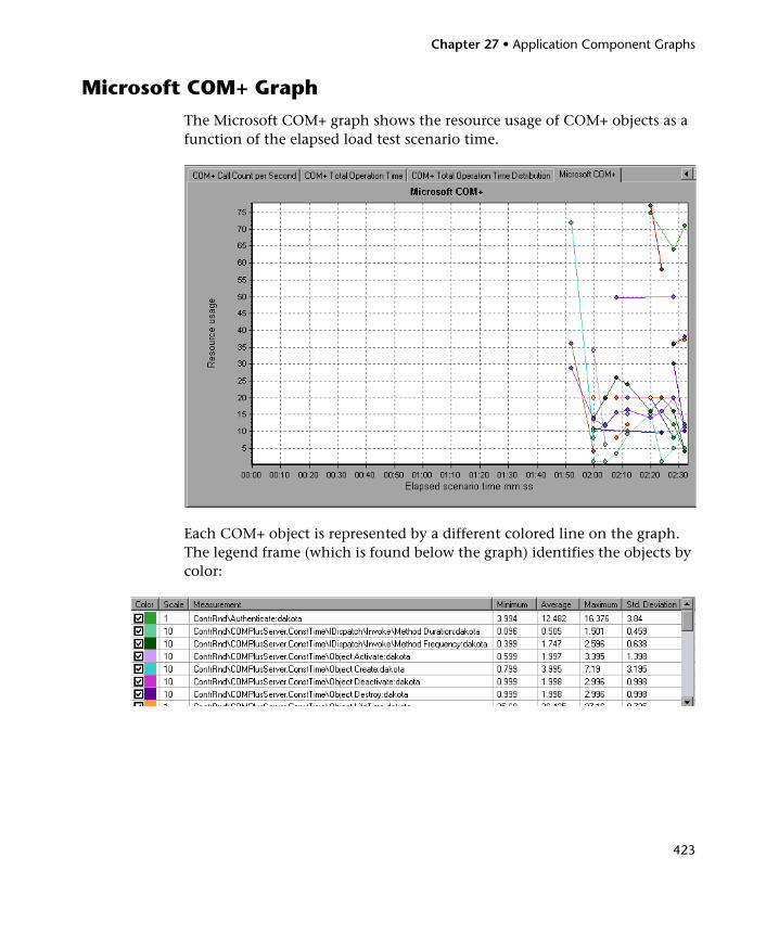
Chapter 27 • Application Component Graphs
423
Microsoft COM+ Graph
The Microsoft COM+ graph shows the resource usage of COM+ objects as a function of the elapsed load test scenario time.
Each COM+ object is represented by a different colored line on the graph. The legend frame (which is found below the graph) identifies the objects by color:
Chapter 27 • Application Component Graphs
424
The following tables describe the default counters that can be measured:
Authentication Metrics
Application Events
Thread Events
Measurement Description
Authenticate Frequency of successful method call level authentication. When you set an authentication level for an application, you determine what degree of authentication is performed when clients call into the application.
Authenticate Failed Frequency of failed method call level authentication.
Measurement Description
Activation Frequency of application activation or startup.
Shutdown Frequency of application shutdown or termination.
Measurement Description
Thread Start Rate at which single-threaded apartment (STA) thread for application have been started.
Thread Terminate Rate at which single-threaded apartment (STA) thread for application have been terminated.
Work Enque Event sent if a work is queued in single thread apartment object (STA). Note: These events are not signaled/sent in Windows Server 2003 and later.
Work Reject Event sent if a work is rejected from single thread apartment object (STA). Note: These events are not signaled/sent in Windows Server 2003 and later.

Chapter 27 • Application Component Graphs
425
Transaction Events
Object Events
Measurement Description
Transaction Duration Duration of COM+ transactions for selected application.
Transaction Start Rate at which transactions have started.
Transaction Prepared Rate at which transactions have completed the prepare phase of the two-phase protocol.
Transaction Aborted Rate at which transactions have been aborted.
Transaction Commit Rate at which transactions have completed the commit protocol.
Measurement Description
Object Life Time Duration of object existence (from instantiation to destruction).
Object Create Rate at which new instances of this object are created.
Object Destroy Rate at which instances of the object are destroyed.
Object Activate Rate of retrieving instances of a new JIT-activated object.
Object Deactivation Rate of freeing JIT-activated object via SetComplete or SetAbort.
Disable Commit Rate of client calls to DisableCommit on a context. DisableCommit declares that the object’s transactional updates are inconsistent and can’t be committed in their present state.
Chapter 27 • Application Component Graphs
426
Method Events
Enable Commit Rate of client calls to EnableCommit on a context. EnableCommit declares that the current object’s work is not necessarily finished, but that its transactional updates are consistent and could be committed in their present form.
Set Complete Rate of client calls to SetComplete on a context. SetComplete declares that the transaction in which the object is executing can be committed, and that the object should be deactivated on returning from the currently executing method call.
Set Abort Rate of client calls to SetAbort on a context. SetAbort declares that the transaction in which the object is executing must be aborted, and that the object should be deactivated on returning from the currently executing method call.
Measurement Description
Method Duration Average duration of method.
Method Frequency Frequency of method invocation.
Method Failed Frequency of failed methods (i.e. methods that return error HRESULT codes).
Method Exceptions Frequency of exceptions thrown by selected method.
Measurement Description
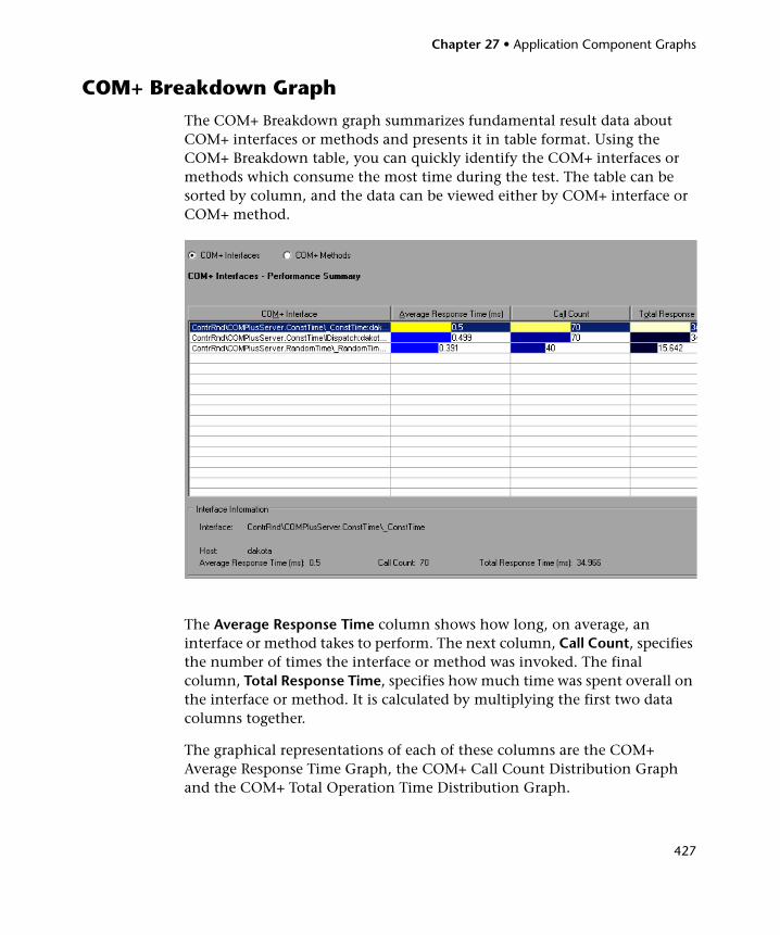
Chapter 27 • Application Component Graphs
427
COM+ Breakdown Graph
The COM+ Breakdown graph summarizes fundamental result data about COM+ interfaces or methods and presents it in table format. Using the COM+ Breakdown table, you can quickly identify the COM+ interfaces or methods which consume the most time during the test. The table can be sorted by column, and the data can be viewed either by COM+ interface or COM+ method.
The Average Response Time column shows how long, on average, an interface or method takes to perform. The next column, Call Count, specifies the number of times the interface or method was invoked. The final column, Total Response Time, specifies how much time was spent overall on the interface or method. It is calculated by multiplying the first two data columns together.
The graphical representations of each of these columns are the COM+ Average Response Time Graph, the COM+ Call Count Distribution Graph and the COM+ Total Operation Time Distribution Graph.
Chapter 27 • Application Component Graphs
428
Interfaces are listed in the COM+ Interface column in the form Interface:Host. In the table above, the _ConstTime interface took an average of .5 seconds to execute and was called 70 times. Overall, this interface took 34.966 seconds to execute.
To sort the list by a column, click on the column heading. The list above is sorted by Average Response Time which contains the triangle icon specifying a sort in descending order.
Viewing COM+ Methods
The table initially displays COM+ interfaces, but you can also view the list of COM+ methods.
To view the methods of a selected interface, select the COM+ Methods option. You can also double-click on the interface row to view the methods. The methods of the specified interface are listed in the COM+ Method column.
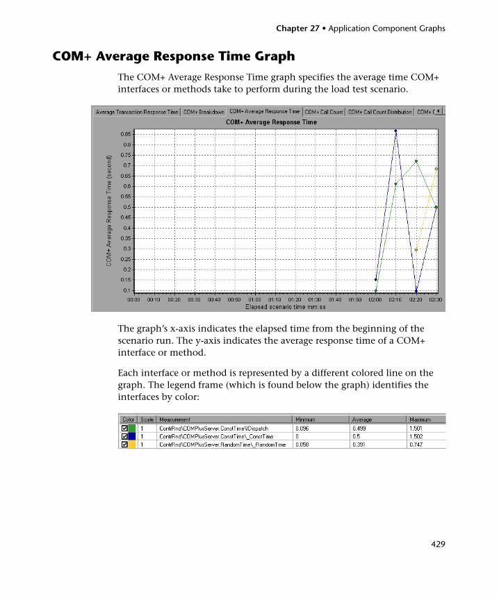
Chapter 27 • Application Component Graphs
429
COM+ Average Response Time Graph
The COM+ Average Response Time graph specifies the average time COM+ interfaces or methods take to perform during the load test scenario.
The graph’s x-axis indicates the elapsed time from the beginning of the scenario run. The y-axis indicates the average response time of a COM+ interface or method.
Each interface or method is represented by a different colored line on the graph. The legend frame (which is found below the graph) identifies the interfaces by color:
Chapter 27 • Application Component Graphs
430
This legend shows that the blue colored line belongs to the COM+ interface _ConstTime. Looking at the graph above, we see that this interface has higher response times than all other COM+ interfaces. At 2:10 minutes into the scenario, it records an average response time of 0.87 seconds.
Note: The 0.87 second data point is an average, taken from all data points recorded within a 10 second interval (the default granularity). You can change the length of this sample interval.
Hint: To highlight a specific interface line in the graph, select the interface row in the legend.
Viewing COM+ Methods
The table initially displays COM+ interfaces, but you can also view the list of COM+ methods by using drill-down or filtering techniques. For more information, see “Filtering and Sorting Graph Data” on page 79 and “Drilling Down in a Graph” on page 102.
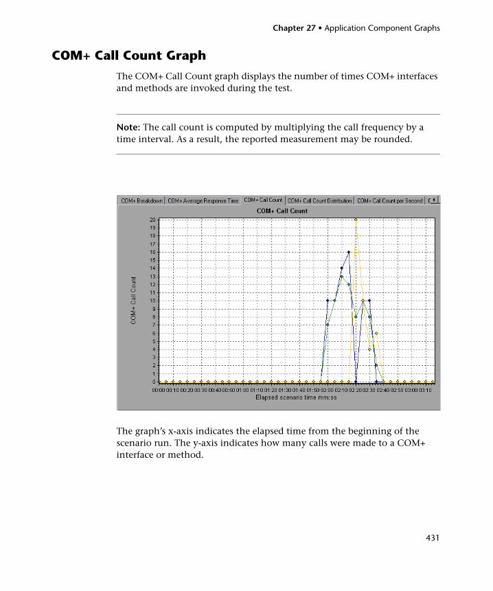
Chapter 27 • Application Component Graphs
431
COM+ Call Count Graph
The COM+ Call Count graph displays the number of times COM+ interfaces and methods are invoked during the test.
Note: The call count is computed by multiplying the call frequency by a time interval. As a result, the reported measurement may be rounded.
The graph’s x-axis indicates the elapsed time from the beginning of the scenario run. The y-axis indicates how many calls were made to a COM+ interface or method.
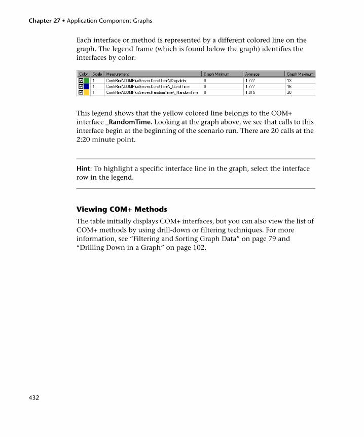
Chapter 27 • Application Component Graphs
432
Each interface or method is represented by a different colored line on the graph. The legend frame (which is found below the graph) identifies the interfaces by color:
This legend shows that the yellow colored line belongs to the COM+ interface _RandomTime. Looking at the graph above, we see that calls to this interface begin at the beginning of the scenario run. There are 20 calls at the 2:20 minute point.
Hint: To highlight a specific interface line in the graph, select the interface row in the legend.
Viewing COM+ Methods
The table initially displays COM+ interfaces, but you can also view the list of COM+ methods by using drill-down or filtering techniques. For more information, see “Filtering and Sorting Graph Data” on page 79 and “Drilling Down in a Graph” on page 102.
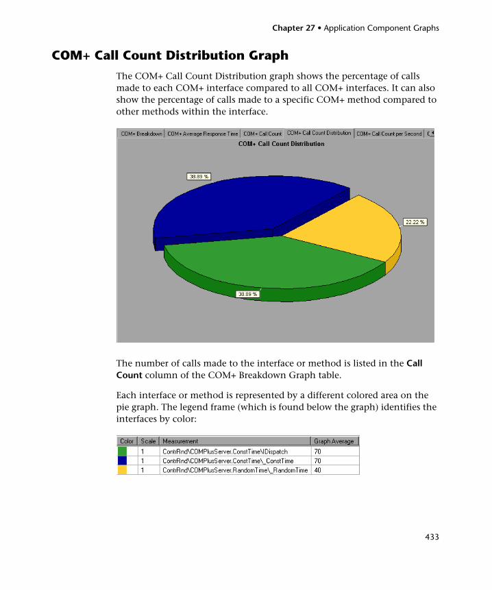
Chapter 27 • Application Component Graphs
433
COM+ Call Count Distribution Graph
The COM+ Call Count Distribution graph shows the percentage of calls made to each COM+ interface compared to all COM+ interfaces. It can also show the percentage of calls made to a specific COM+ method compared to other methods within the interface.
The number of calls made to the interface or method is listed in the Call Count column of the COM+ Breakdown Graph table.
Each interface or method is represented by a different colored area on the pie graph. The legend frame (which is found below the graph) identifies the interfaces by color:
Chapter 27 • Application Component Graphs
434
This legend shows that the green colored area belongs to the COM+ interface IDispatch. Looking at the graph above, we see that 38.89% of calls are made to this interface. The actual figures can be seen in the Call Count column of the COM+ Breakdown Graph table: there are 13 calls to this interface out of a total of 49 calls.
Hint: To highlight a specific interface line in the graph, select the interface row in the legend.
Viewing COM+ Methods
The table initially displays COM+ interfaces, but you can also view the list of COM+ methods by using drill-down or filtering techniques. For more information, see “Filtering and Sorting Graph Data” on page 79 and “Drilling Down in a Graph” on page 102.

Chapter 27 • Application Component Graphs
435
COM+ Call Count Per Second Graph
The COM+ Call Count Per Second graph shows the number of times per second a COM+ interface or method is invoked.
This graph is similar to the COM+ Call Count Graph except that the y-axis indicates how many invocations were made to a COM+ interface or method per second.
Each interface or method is represented by a different colored line on the graph. The legend frame (which is found below the graph) identifies the interfaces by color:
Chapter 27 • Application Component Graphs
436
This legend shows that the green colored line belongs to the COM+ interface IDispatch. Looking at the graph above, we see that calls to this interface begins 1:55 minutes into the scenario run. There is an average of 2.5 calls per second at the 2:10 minute mark.
Hint: To highlight a specific interface line in the graph, select the interface row in the legend.
Viewing COM+ Methods
To view the average response time of the individual methods within a COM+ interface, see “Filtering and Sorting Graph Data” on page 79 and “Drilling Down in a Graph” on page 102.
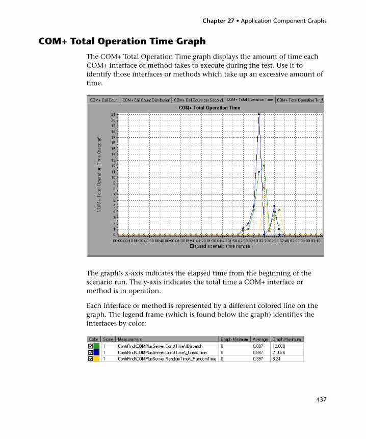
Chapter 27 • Application Component Graphs
437
COM+ Total Operation Time Graph
The COM+ Total Operation Time graph displays the amount of time each COM+ interface or method takes to execute during the test. Use it to identify those interfaces or methods which take up an excessive amount of time.
The graph’s x-axis indicates the elapsed time from the beginning of the scenario run. The y-axis indicates the total time a COM+ interface or method is in operation.
Each interface or method is represented by a different colored line on the graph. The legend frame (which is found below the graph) identifies the interfaces by color:
Chapter 27 • Application Component Graphs
438
This legend shows that the blue colored line belongs to the COM+ interface _ConstTime. Looking at the graph above, we see that throughout the scenario, this interface consumes more time than any other, especially at 2 minutes and 15 seconds into the scenario run, where the calls to this interface take an average of 21 seconds.
Hint: To highlight a specific interface line in the graph, select the interface row in the legend.
Viewing COM+ Methods
The table initially displays COM+ interfaces, but you can also view the list of COM+ methods by using drill-down or filtering techniques. For more information, see “Filtering and Sorting Graph Data” on page 79 and “Drilling Down in a Graph” on page 102.
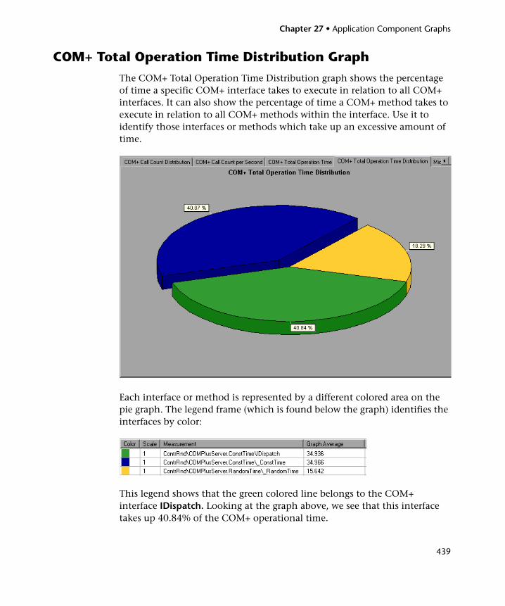
Chapter 27 • Application Component Graphs
439
COM+ Total Operation Time Distribution Graph
The COM+ Total Operation Time Distribution graph shows the percentage of time a specific COM+ interface takes to execute in relation to all COM+ interfaces. It can also show the percentage of time a COM+ method takes to execute in relation to all COM+ methods within the interface. Use it to identify those interfaces or methods which take up an excessive amount of time.
Each interface or method is represented by a different colored area on the pie graph. The legend frame (which is found below the graph) identifies the interfaces by color:
This legend shows that the green colored line belongs to the COM+ interface IDispatch. Looking at the graph above, we see that this interface takes up 40.84% of the COM+ operational time.
Chapter 27 • Application Component Graphs
440
Hint: To highlight a specific interface line in the graph, select the interface row in the legend.
Viewing COM+ Methods
To view the average response time of the individual methods within a COM+ interface, see “Filtering and Sorting Graph Data” on page 79 and “Drilling Down in a Graph” on page 102.
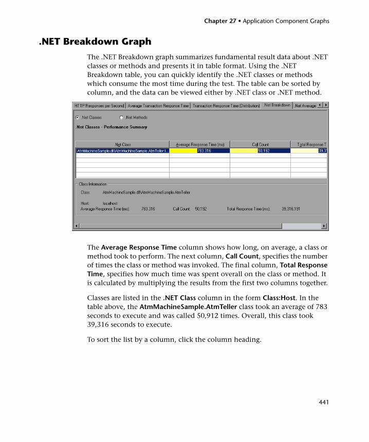
Chapter 27 • Application Component Graphs
441
.NET Breakdown Graph
The .NET Breakdown graph summarizes fundamental result data about .NET classes or methods and presents it in table format. Using the .NET Breakdown table, you can quickly identify the .NET classes or methods which consume the most time during the test. The table can be sorted by column, and the data can be viewed either by .NET class or .NET method.
The Average Response Time column shows how long, on average, a class or method took to perform. The next column, Call Count, specifies the number of times the class or method was invoked. The final column, Total Response Time, specifies how much time was spent overall on the class or method. It is calculated by multiplying the results from the first two columns together.
Classes are listed in the .NET Class column in the form Class:Host. In the table above, the AtmMachineSample.AtmTeller class took an average of 783 seconds to execute and was called 50,912 times. Overall, this class took 39,316 seconds to execute.
To sort the list by a column, click the column heading.

Chapter 27 • Application Component Graphs
442
Each column in the .NET Breakdown graph is graphically represented by another graph, as described in the following table:
The table initially displays .NET classes, but you can also view the list of .NET methods. To view .NET methods, select the .NET Methods option, or double-click the class row. The methods of the specified class are listed in the .NET Method column.
.NET Breakdown Column Graphical Representation
Average Response Time .NET Average Response Time Graph
Call Count .NET Call Count Graph
Total Response Time .NET Total Operation Time Distribution Graph
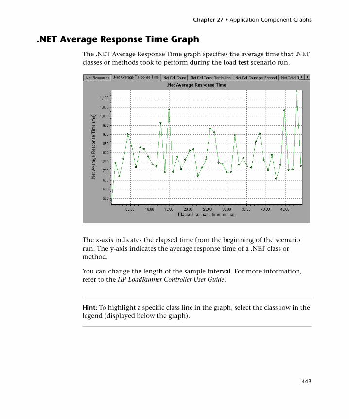
Chapter 27 • Application Component Graphs
443
.NET Average Response Time Graph
The .NET Average Response Time graph specifies the average time that .NET classes or methods took to perform during the load test scenario run.
The x-axis indicates the elapsed time from the beginning of the scenario run. The y-axis indicates the average response time of a .NET class or method.
You can change the length of the sample interval. For more information, refer to the HP LoadRunner Controller User Guide.
Hint: To highlight a specific class line in the graph, select the class row in the legend (displayed below the graph).
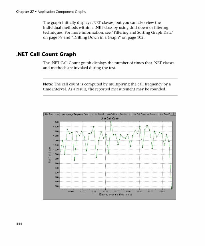
Chapter 27 • Application Component Graphs
444
The graph initially displays .NET classes, but you can also view the individual methods within a .NET class by using drill-down or filtering techniques. For more information, see “Filtering and Sorting Graph Data” on page 79 and “Drilling Down in a Graph” on page 102.
.NET Call Count Graph
The .NET Call Count graph displays the number of times that .NET classes and methods are invoked during the test.
Note: The call count is computed by multiplying the call frequency by a time interval. As a result, the reported measurement may be rounded.
Chapter 27 • Application Component Graphs
445
The x-axis indicates the elapsed time from the beginning of the scenario run. The y-axis indicates how many calls were made to a .NET class or method.
Hint: To highlight a specific class line in the graph, select the class row in the legend (displayed below the graph).
The graph initially displays .NET classes, but you can also view the individual methods within a .NET class by using drill-down or filtering techniques. For more information, see “Filtering and Sorting Graph Data” on page 79 and “Drilling Down in a Graph” on page 102.
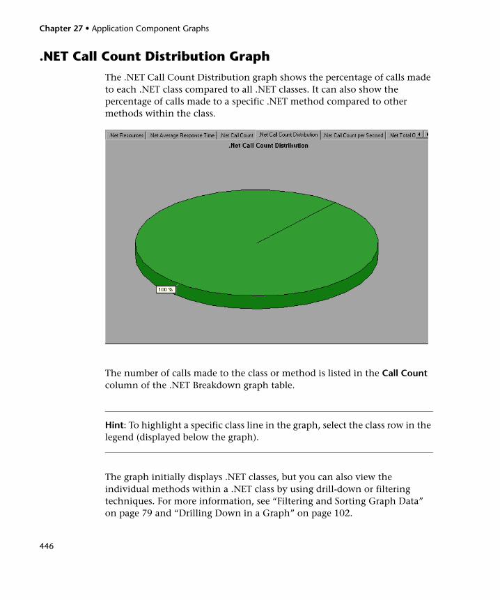
Chapter 27 • Application Component Graphs
446
.NET Call Count Distribution Graph
The .NET Call Count Distribution graph shows the percentage of calls made to each .NET class compared to all .NET classes. It can also show the percentage of calls made to a specific .NET method compared to other methods within the class.
The number of calls made to the class or method is listed in the Call Count column of the .NET Breakdown graph table.
Hint: To highlight a specific class line in the graph, select the class row in the legend (displayed below the graph).
The graph initially displays .NET classes, but you can also view the individual methods within a .NET class by using drill-down or filtering techniques. For more information, see “Filtering and Sorting Graph Data” on page 79 and “Drilling Down in a Graph” on page 102.
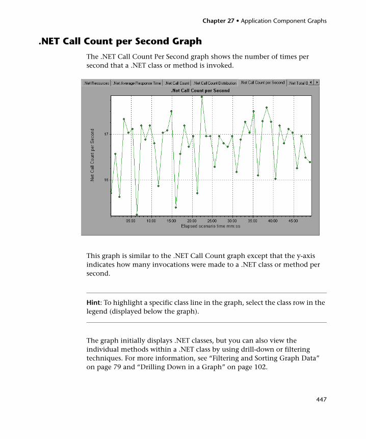
Chapter 27 • Application Component Graphs
447
.NET Call Count per Second Graph
The .NET Call Count Per Second graph shows the number of times per second that a .NET class or method is invoked.
This graph is similar to the .NET Call Count graph except that the y-axis indicates how many invocations were made to a .NET class or method per second.
Hint: To highlight a specific class line in the graph, select the class row in the legend (displayed below the graph).
The graph initially displays .NET classes, but you can also view the individual methods within a .NET class by using drill-down or filtering techniques. For more information, see “Filtering and Sorting Graph Data” on page 79 and “Drilling Down in a Graph” on page 102.
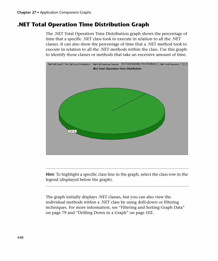
Chapter 27 • Application Component Graphs
448
.NET Total Operation Time Distribution Graph
The .NET Total Operation Time Distribution graph shows the percentage of time that a specific .NET class took to execute in relation to all the .NET classes. It can also show the percentage of time that a .NET method took to execute in relation to all the .NET methods within the class. Use this graph to identify those classes or methods that take an excessive amount of time.
Hint: To highlight a specific class line in the graph, select the class row in the legend (displayed below the graph).
The graph initially displays .NET classes, but you can also view the individual methods within a .NET class by using drill-down or filtering techniques. For more information, see “Filtering and Sorting Graph Data” on page 79 and “Drilling Down in a Graph” on page 102.
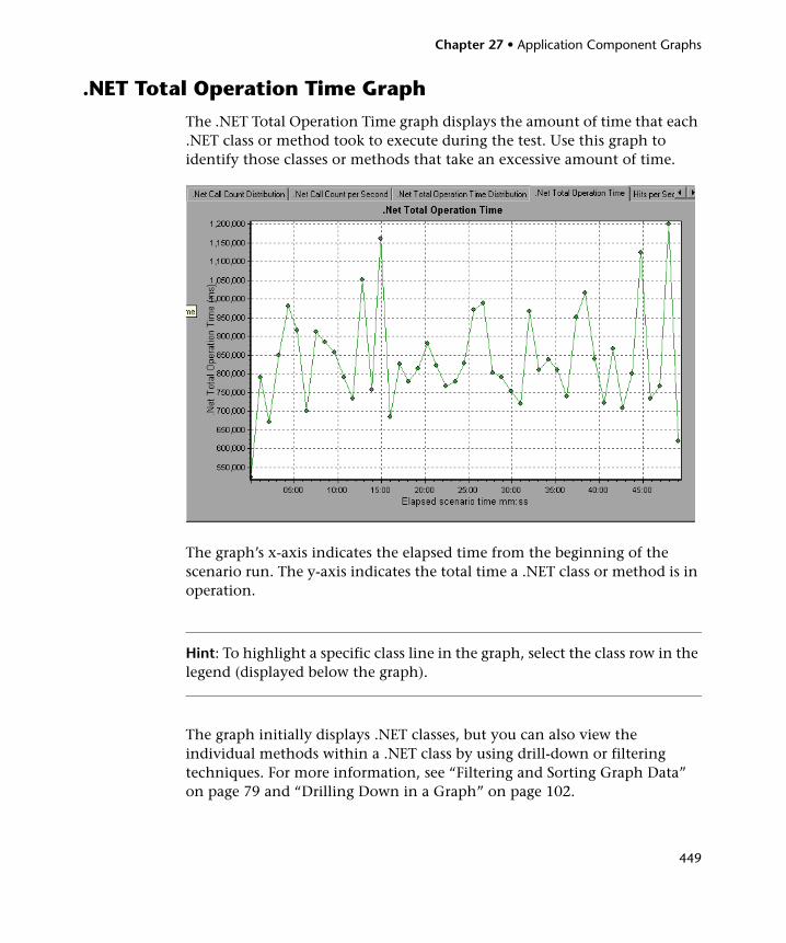
Chapter 27 • Application Component Graphs
449
.NET Total Operation Time Graph
The .NET Total Operation Time graph displays the amount of time that each .NET class or method took to execute during the test. Use this graph to identify those classes or methods that take an excessive amount of time.
The graph’s x-axis indicates the elapsed time from the beginning of the scenario run. The y-axis indicates the total time a .NET class or method is in operation.
Hint: To highlight a specific class line in the graph, select the class row in the legend (displayed below the graph).
The graph initially displays .NET classes, but you can also view the individual methods within a .NET class by using drill-down or filtering techniques. For more information, see “Filtering and Sorting Graph Data” on page 79 and “Drilling Down in a Graph” on page 102.
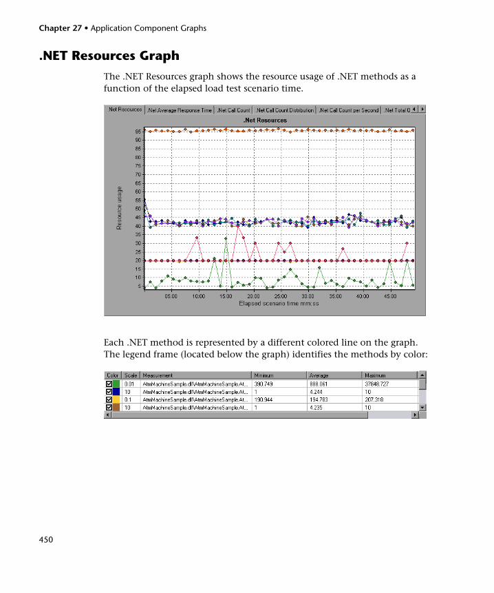
Chapter 27 • Application Component Graphs
450
.NET Resources Graph
The .NET Resources graph shows the resource usage of .NET methods as a function of the elapsed load test scenario time.
Each .NET method is represented by a different colored line on the graph. The legend frame (located below the graph) identifies the methods by color:
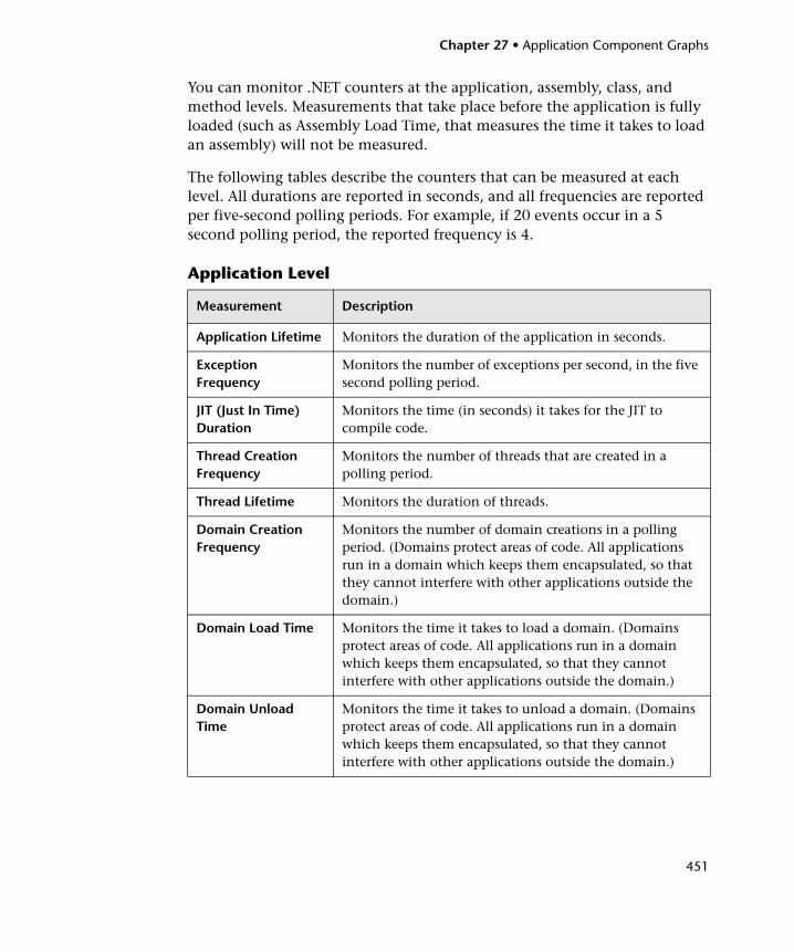
Chapter 27 • Application Component Graphs
451
You can monitor .NET counters at the application, assembly, class, and method levels. Measurements that take place before the application is fully loaded (such as Assembly Load Time, that measures the time it takes to load an assembly) will not be measured.
The following tables describe the counters that can be measured at each level. All durations are reported in seconds, and all frequencies are reported per five-second polling periods. For example, if 20 events occur in a 5 second polling period, the reported frequency is 4.
Application Level
Measurement Description
Application Lifetime Monitors the duration of the application in seconds.
Exception Frequency
Monitors the number of exceptions per second, in the five second polling period.
JIT (Just In Time) Duration
Monitors the time (in seconds) it takes for the JIT to compile code.
Thread Creation Frequency
Monitors the number of threads that are created in a polling period.
Thread Lifetime Monitors the duration of threads.
Domain Creation Frequency
Monitors the number of domain creations in a polling period. (Domains protect areas of code. All applications run in a domain which keeps them encapsulated, so that they cannot interfere with other applications outside the domain.)
Domain Load Time Monitors the time it takes to load a domain. (Domains protect areas of code. All applications run in a domain which keeps them encapsulated, so that they cannot interfere with other applications outside the domain.)
Domain Unload Time
Monitors the time it takes to unload a domain. (Domains protect areas of code. All applications run in a domain which keeps them encapsulated, so that they cannot interfere with other applications outside the domain.)
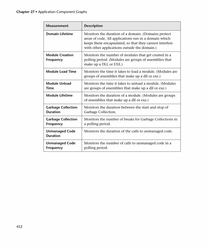
Chapter 27 • Application Component Graphs
452
Domain Lifetime Monitors the duration of a domain. (Domains protect areas of code. All applications run in a domain which keeps them encapsulated, so that they cannot interfere with other applications outside the domain.)
Module Creation Frequency
Monitors the number of modules that get created in a polling period. (Modules are groups of assemblies that make up a DLL or EXE.)
Module Load Time Monitors the time it takes to load a module. (Modules are groups of assemblies that make up a dll or exe.)
Module Unload Time
Monitors the time it takes to unload a module. (Modules are groups of assemblies that make up a dll or exe.)
Module Lifetime Monitors the duration of a module. (Modules are groups of assemblies that make up a dll or exe.)
Garbage Collection Duration
Monitors the duration between the start and stop of Garbage Collection.
Garbage Collection Frequency
Monitors the number of breaks for Garbage Collections in a polling period.
Unmanaged Code Duration
Monitors the duration of the calls to unmanaged code.
Unmanaged Code Frequency
Monitors the number of calls to unmanaged code in a polling period.
Measurement Description
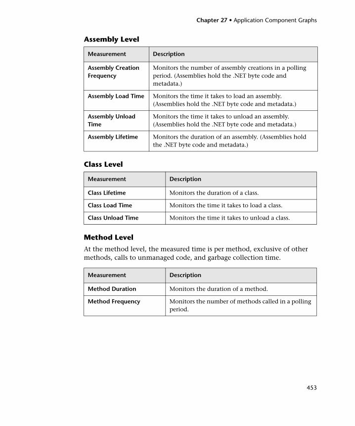
Chapter 27 • Application Component Graphs
453
Assembly Level
Class Level
Method Level
At the method level, the measured time is per method, exclusive of other methods, calls to unmanaged code, and garbage collection time.
Measurement Description
Assembly Creation Frequency
Monitors the number of assembly creations in a polling period. (Assemblies hold the .NET byte code and metadata.)
Assembly Load Time Monitors the time it takes to load an assembly. (Assemblies hold the .NET byte code and metadata.)
Assembly Unload Time
Monitors the time it takes to unload an assembly. (Assemblies hold the .NET byte code and metadata.)
Assembly Lifetime Monitors the duration of an assembly. (Assemblies hold the .NET byte code and metadata.)
Measurement Description
Class Lifetime Monitors the duration of a class.
Class Load Time Monitors the time it takes to load a class.
Class Unload Time Monitors the time it takes to unload a class.
Measurement Description
Method Duration Monitors the duration of a method.
Method Frequency Monitors the number of methods called in a polling period.

Chapter 27 • Application Component Graphs
454
455
28 Application Deployment Solutions Graphs
After a load test scenario run, you use the Application Deployment Solutions graphs to analyze Citrix MetaFrame XP server performance.
This chapter includes:
➤ About Application Deployment Solutions Graphs on page 455
➤ Citrix MetaFrame XP Graph on page 456
About Application Deployment Solutions Graphs
LoadRunner’s Citrix MetaFrame XP monitor provides you with information about the application deployment usage of the Citrix MetaFrame XP server during a load test scenario execution. In order to obtain performance data, before you execute the scenario you need to activate the online monitor for the server and specify which resources you want to measure.
For more information on activating and configuring the Application Deployment Solutions monitor, refer to the HP LoadRunner Controller User Guide.
Chapter 28 • Application Deployment Solutions Graphs
456
Citrix MetaFrame XP Graph
Citrix MetaFrame is an Application Deployment solution which delivers applications across networks. The Citrix MetaFrame Resource Monitor is an Application Deployment Solution monitor, which provides performance information for the Citrix MetaFrame server.
The Citrix MetaFrame XP graph displays statistics about resource usage on the Citrix server during the load test scenario run.
Note: To obtain data for this graph, you need to enable the Citrix MetaFrame XP monitor (from the Controller) and select the default measurements you want to display, before running the scenario.
Chapter 28 • Application Deployment Solutions Graphs
457
The following Citrix measurements are available:
Non-Virtual Counters
Measurement Description
% Disk Time The percentage of elapsed time that the selected disk drive services read or write requests.
% Processor Time The percentage of time that the processor executes a non-Idle thread. This counter is a primary indicator of processor activity. It is calculated by measuring the time that the processor spends executing the thread of the Idle process in each sample interval, and subtracting that value from 100%. (Each processor has an Idle thread which consumes cycles when no other threads are ready to run.) It can be viewed as the percentage of the sample interval spent doing useful work. This counter displays the average percentage of busy time observed during the sample interval. It is calculated by monitoring the time the service was inactive, and then subtracting that value from 100%.
File data Operations/sec The rate that the computer issues Read and Write operations to file system devices. It does not include File Control Operations.
Chapter 28 • Application Deployment Solutions Graphs
458
Interrupts/sec The average number of hardware interrupts the processor receives and services per second. It does not include DPCs, which are counted separately. This value is an indirect indicator of the activity of devices that generate interrupts, such as the system clock, the mouse, disk drivers, data communication lines, network interface cards and other peripheral devices. These devices normally interrupt the processor when they have completed a task or require attention. Normal thread execution is suspended during interrupts. Most system clocks interrupt the processor every 10 milliseconds, creating a background of interrupt activity. This counter displays the difference between the values observed in the last two samples, divided by the duration of the sample interval.
Output Session Line Speed This value represents the line speed from server to client for a session in bps.
Input Session Line Speed This value represents the line speed from client to server for a session in bps.
Page Faults/sec A count of the Page Faults in the processor. A page fault occurs when a process refers to a virtual memory page that is not in its Working Set in main memory. A Page Fault will not cause the page to be fetched from disk if that page is on the standby list, and hence already in main memory, or if it is in use by another process with whom the page is shared.
Measurement Description
Chapter 28 • Application Deployment Solutions Graphs
459
Pages/sec The number of pages read from the disk or written to the disk to resolve memory references to pages that were not in memory at the time of the reference. This is the sum of Pages Input/sec and Pages Output/sec. This counter includes paging traffic on behalf of the system Cache to access file data for applications. This value also includes the pages to/from non-cached mapped memory files. This is the primary counter to observe if you are concerned about excessive memory pressure (that is, thrashing), and the excessive paging that may result.
Pool Nonpaged Bytes The number of bytes in the Nonpaged Pool, a system memory area where space is acquired by operating system components as they accomplish their appointed tasks. Nonpaged Pool pages cannot be paged out to the paging file, but instead remain in main memory as long as they are allocated.
Private Bytes The current number of bytes this process has allocated that cannot be shared with other processes.
Processor Queue Length The instantaneous length of the processor queue in units of threads. This counter is always 0 unless you are also monitoring a thread counter. All processors use a single queue in which threads wait for processor cycles. This length does not include the threads that are currently executing. A sustained processor queue length greater than two generally indicates processor congestion. This is an instantaneous count, not an average over the time interval.
Threads The number of threads in the computer at the time of data collection. Notice that this is an instantaneous count, not an average over the time interval. A thread is the basic executable entity that can execute instructions in a processor.
Latency – Session Average The average client latency over the life of a session.
Measurement Description
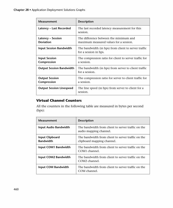
Chapter 28 • Application Deployment Solutions Graphs
460
Virtual Channel Counters
All the counters in the following table are measured in bytes per second (bps):
Latency – Last Recorded The last recorded latency measurement for this session.
Latency – Session Deviation
The difference between the minimum and maximum measured values for a session.
Input Session Bandwidth The bandwidth (in bps) from client to server traffic for a session in bps.
Input Session Compression
The compression ratio for client to server traffic for a session.
Output Session Bandwidth The bandwidth (in bps) from server to client traffic for a session.
Output Session Compression
The compression ratio for server to client traffic for a session.
Output Session Linespeed The line speed (in bps) from server to client for a session.
Measurement Description
Input Audio Bandwidth The bandwidth from client to server traffic on the audio mapping channel.
Input Clipboard Bandwidth
The bandwidth from client to server traffic on the clipboard mapping channel.
Input COM1 Bandwidth The bandwidth from client to server traffic on the COM1 channel.
Input COM2 Bandwidth The bandwidth from client to server traffic on the COM2 channel.
Input COM Bandwidth The bandwidth from client to server traffic on the COM channel.
Measurement Description
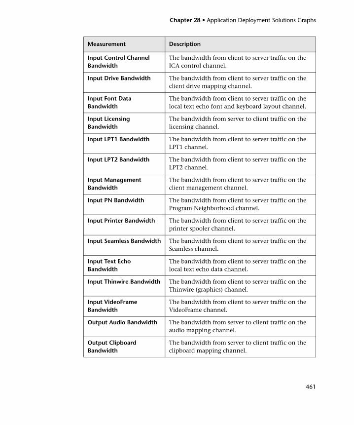
Chapter 28 • Application Deployment Solutions Graphs
461
Input Control Channel Bandwidth
The bandwidth from client to server traffic on the ICA control channel.
Input Drive Bandwidth The bandwidth from client to server traffic on the client drive mapping channel.
Input Font Data Bandwidth
The bandwidth from client to server traffic on the local text echo font and keyboard layout channel.
Input Licensing Bandwidth
The bandwidth from server to client traffic on the licensing channel.
Input LPT1 Bandwidth The bandwidth from client to server traffic on the LPT1 channel.
Input LPT2 Bandwidth The bandwidth from client to server traffic on the LPT2 channel.
Input Management Bandwidth
The bandwidth from client to server traffic on the client management channel.
Input PN Bandwidth The bandwidth from client to server traffic on the Program Neighborhood channel.
Input Printer Bandwidth The bandwidth from client to server traffic on the printer spooler channel.
Input Seamless Bandwidth The bandwidth from client to server traffic on the Seamless channel.
Input Text Echo Bandwidth
The bandwidth from client to server traffic on the local text echo data channel.
Input Thinwire Bandwidth The bandwidth from client to server traffic on the Thinwire (graphics) channel.
Input VideoFrame Bandwidth
The bandwidth from client to server traffic on the VideoFrame channel.
Output Audio Bandwidth The bandwidth from server to client traffic on the audio mapping channel.
Output Clipboard Bandwidth
The bandwidth from server to client traffic on the clipboard mapping channel.
Measurement Description
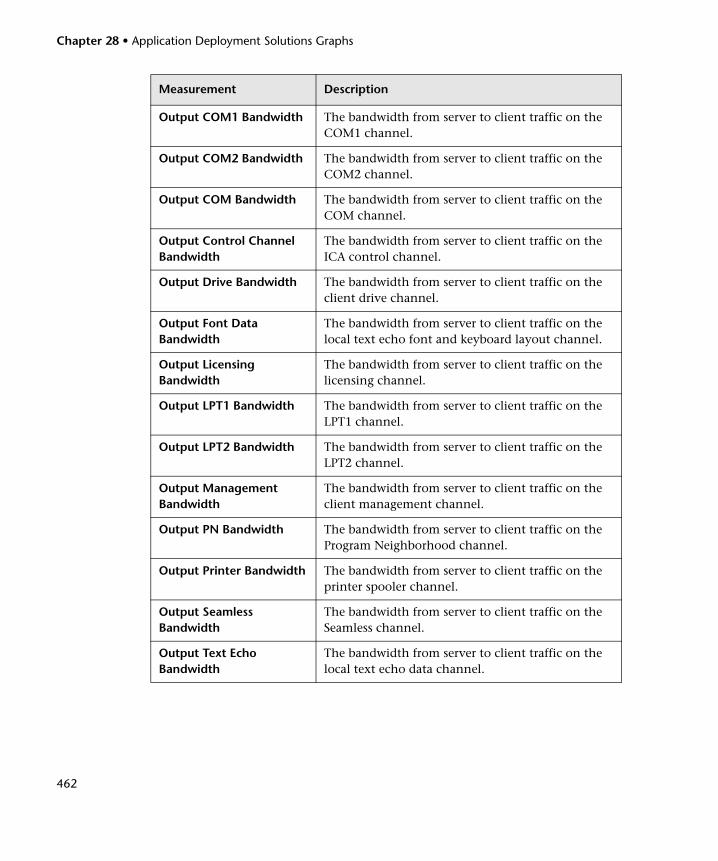
Chapter 28 • Application Deployment Solutions Graphs
462
Output COM1 Bandwidth The bandwidth from server to client traffic on the COM1 channel.
Output COM2 Bandwidth The bandwidth from server to client traffic on the COM2 channel.
Output COM Bandwidth The bandwidth from server to client traffic on the COM channel.
Output Control Channel Bandwidth
The bandwidth from server to client traffic on the ICA control channel.
Output Drive Bandwidth The bandwidth from server to client traffic on the client drive channel.
Output Font Data Bandwidth
The bandwidth from server to client traffic on the local text echo font and keyboard layout channel.
Output Licensing Bandwidth
The bandwidth from server to client traffic on the licensing channel.
Output LPT1 Bandwidth The bandwidth from server to client traffic on the LPT1 channel.
Output LPT2 Bandwidth The bandwidth from server to client traffic on the LPT2 channel.
Output Management Bandwidth
The bandwidth from server to client traffic on the client management channel.
Output PN Bandwidth The bandwidth from server to client traffic on the Program Neighborhood channel.
Output Printer Bandwidth The bandwidth from server to client traffic on the printer spooler channel.
Output Seamless Bandwidth
The bandwidth from server to client traffic on the Seamless channel.
Output Text Echo Bandwidth
The bandwidth from server to client traffic on the local text echo data channel.
Measurement Description
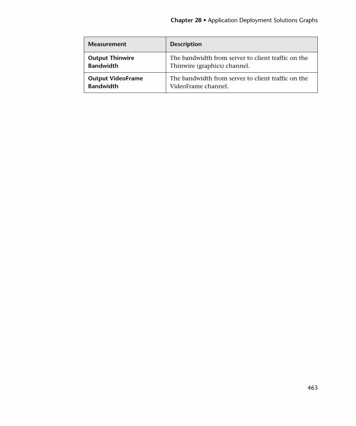
Chapter 28 • Application Deployment Solutions Graphs
463
Output Thinwire Bandwidth
The bandwidth from server to client traffic on the Thinwire (graphics) channel.
Output VideoFrame Bandwidth
The bandwidth from server to client traffic on the VideoFrame channel.
Measurement Description

Chapter 28 • Application Deployment Solutions Graphs
464
465
29 Middleware Performance Graphs
After a load test scenario run, you can use the Middleware Performance monitor graphs to analyze the performance of the Tuxedo and IBM WebSphere MQ Servers.
This chapter includes:
➤ About Middleware Performance Graphs on page 465
➤ Tuxedo Resources Graph on page 466
➤ IBM WebSphere MQ Graph on page 469
About Middleware Performance Graphs
A primary factor in a transaction’s response time is the middleware performance usage. LoadRunner’s Middleware Performance monitors provide you with information about the middleware performance usage of the Tuxedo and IBM WebSphere MQ servers during a load test scenario execution. To obtain performance data, you need to activate the online monitor for the server and specify which resources you want to measure before executing the scenario.
For more information on activating and configuring the Middleware Performance monitors, refer to the HP LoadRunner Controller User Guide.
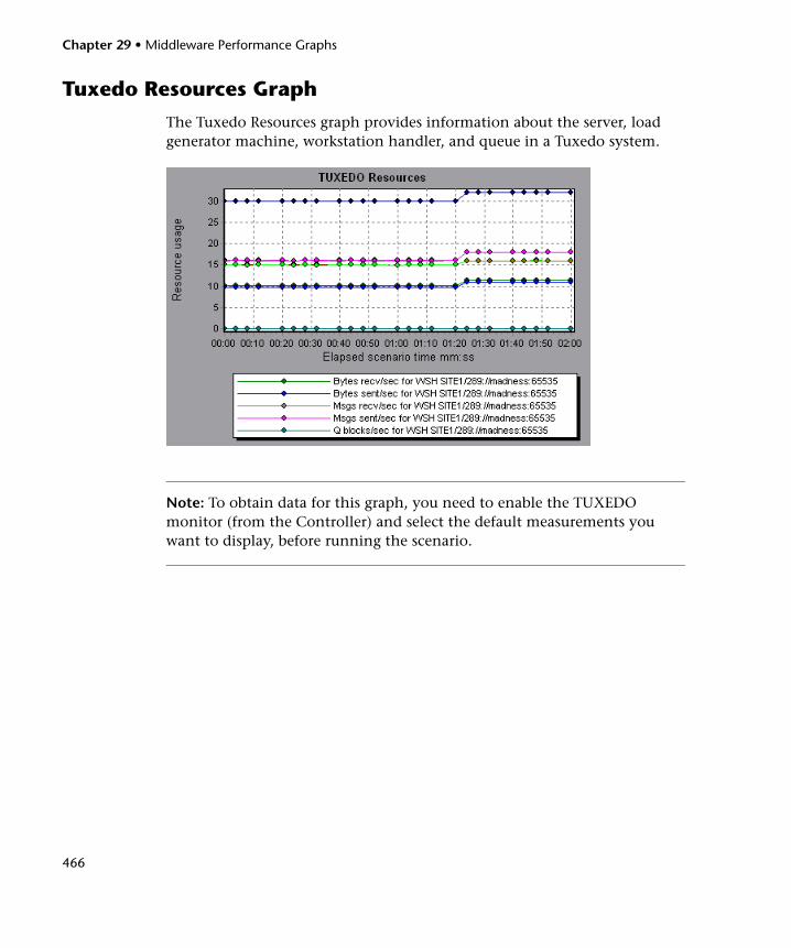
Chapter 29 • Middleware Performance Graphs
466
Tuxedo Resources Graph
The Tuxedo Resources graph provides information about the server, load generator machine, workstation handler, and queue in a Tuxedo system.
Note: To obtain data for this graph, you need to enable the TUXEDO monitor (from the Controller) and select the default measurements you want to display, before running the scenario.
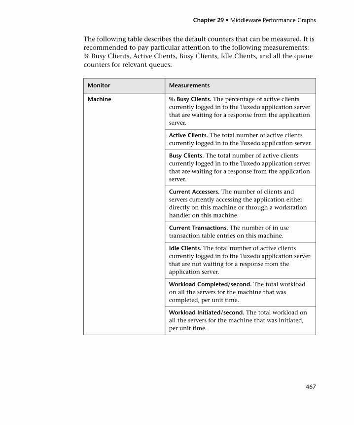
Chapter 29 • Middleware Performance Graphs
467
The following table describes the default counters that can be measured. It is recommended to pay particular attention to the following measurements: % Busy Clients, Active Clients, Busy Clients, Idle Clients, and all the queue counters for relevant queues.
Monitor Measurements
Machine % Busy Clients. The percentage of active clients currently logged in to the Tuxedo application server that are waiting for a response from the application server.
Active Clients. The total number of active clients currently logged in to the Tuxedo application server.
Busy Clients. The total number of active clients currently logged in to the Tuxedo application server that are waiting for a response from the application server.
Current Accessers. The number of clients and servers currently accessing the application either directly on this machine or through a workstation handler on this machine.
Current Transactions. The number of in use transaction table entries on this machine.
Idle Clients. The total number of active clients currently logged in to the Tuxedo application server that are not waiting for a response from the application server.
Workload Completed/second. The total workload on all the servers for the machine that was completed, per unit time.
Workload Initiated/second. The total workload on all the servers for the machine that was initiated, per unit time.

Chapter 29 • Middleware Performance Graphs
468
Queue % Busy Servers. The percentage of active servers currently handling Tuxedo requests.
Active Servers. The total number of active servers either handling or waiting to handle Tuxedo requests.
Busy Servers. The total number of active servers currently busy handling Tuxedo requests.
Idle Servers. The total number of active servers currently waiting to handle Tuxedo requests.
Number Queued. The total number of messages which have been placed on the queue.
Server Requests/second. The number of server requests handled per second.
Workload/second. The workload is a weighted measure of the server requests. Some requests could have a different weight than others. By default, the workload is always 50 times the number of requests.
Workstation Handler (WSH)
Bytes Received/sec. The total number of bytes received by the workstation handler, per second.
Bytes Sent/sec. The total number of bytes sent back to the clients by the workstation handler, per second.
Messages Received/sec. The number of messages received by the workstation handler, per second.
Messages Sent/sec. The number of messages sent back to the clients by the workstation handler, per second.
Number of Queue Blocks/sec. The number of times the queue for the workstation handler blocked, per second. This gives an idea of how often the workstation handler was overloaded.
Monitor Measurements
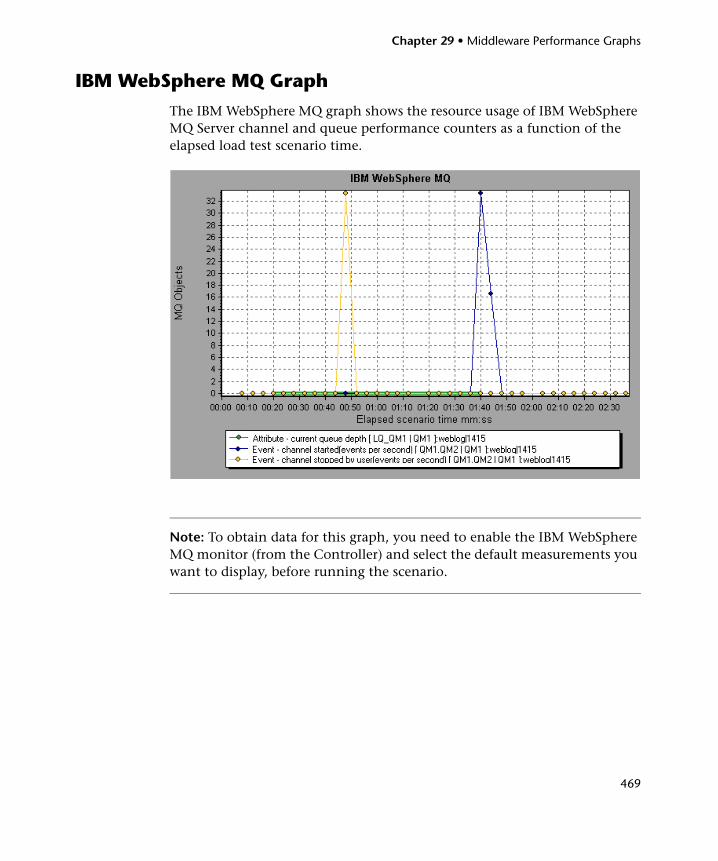
Chapter 29 • Middleware Performance Graphs
469
IBM WebSphere MQ Graph
The IBM WebSphere MQ graph shows the resource usage of IBM WebSphere MQ Server channel and queue performance counters as a function of the elapsed load test scenario time.
Note: To obtain data for this graph, you need to enable the IBM WebSphere MQ monitor (from the Controller) and select the default measurements you want to display, before running the scenario.
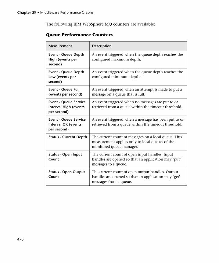
Chapter 29 • Middleware Performance Graphs
470
The following IBM WebSphere MQ counters are available:
Queue Performance Counters
Measurement Description
Event - Queue Depth High (events per second)
An event triggered when the queue depth reaches the configured maximum depth.
Event - Queue Depth Low (events per second)
An event triggered when the queue depth reaches the configured minimum depth.
Event - Queue Full (events per second)
An event triggered when an attempt is made to put a message on a queue that is full.
Event - Queue Service Interval High (events per second)
An event triggered when no messages are put to or retrieved from a queue within the timeout threshold.
Event - Queue Service Interval OK (events per second)
An event triggered when a message has been put to or retrieved from a queue within the timeout threshold.
Status - Current Depth The current count of messages on a local queue. This measurement applies only to local queues of the monitored queue manager.
Status - Open Input Count
The current count of open input handles. Input handles are opened so that an application may "put" messages to a queue.
Status - Open Output Count
The current count of open output handles. Output handles are opened so that an application may "get" messages from a queue.
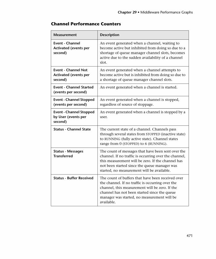
Chapter 29 • Middleware Performance Graphs
471
Channel Performance Counters
Measurement Description
Event - Channel Activated (events per second)
An event generated when a channel, waiting to become active but inhibited from doing so due to a shortage of queue manager channel slots, becomes active due to the sudden availability of a channel slot.
Event - Channel Not Activated (events per second)
An event generated when a channel attempts to become active but is inhibited from doing so due to a shortage of queue manager channel slots.
Event - Channel Started (events per second)
An event generated when a channel is started.
Event - Channel Stopped (events per second)
An event generated when a channel is stopped, regardless of source of stoppage.
Event - Channel Stopped by User (events per second)
An event generated when a channel is stopped by a user.
Status - Channel State The current state of a channel. Channels pass through several states from STOPPED (inactive state) to RUNNING (fully active state). Channel states range from 0 (STOPPED) to 6 (RUNNING).
Status - Messages Transferred
The count of messages that have been sent over the channel. If no traffic is occurring over the channel, this measurement will be zero. If the channel has not been started since the queue manager was started, no measurement will be available.
Status - Buffer Received The count of buffers that have been received over the channel. If no traffic is occurring over the channel, this measurement will be zero. If the channel has not been started since the queue manager was started, no measurement will be available.
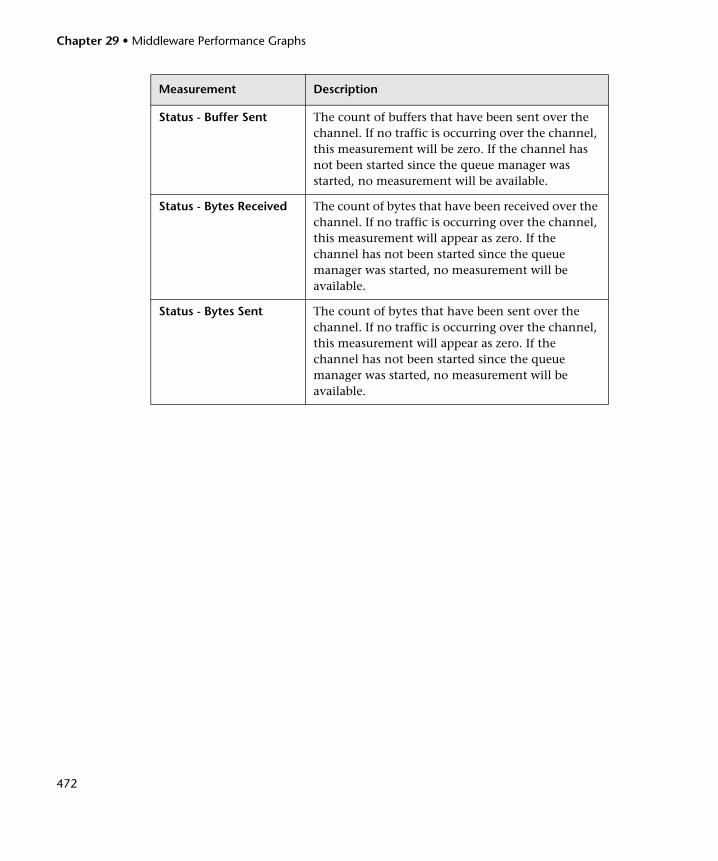
Chapter 29 • Middleware Performance Graphs
472
Status - Buffer Sent The count of buffers that have been sent over the channel. If no traffic is occurring over the channel, this measurement will be zero. If the channel has not been started since the queue manager was started, no measurement will be available.
Status - Bytes Received The count of bytes that have been received over the channel. If no traffic is occurring over the channel, this measurement will appear as zero. If the channel has not been started since the queue manager was started, no measurement will be available.
Status - Bytes Sent The count of bytes that have been sent over the channel. If no traffic is occurring over the channel, this measurement will appear as zero. If the channel has not been started since the queue manager was started, no measurement will be available.
Measurement Description
473
30 Infrastructure Resources Graphs
After running a load test scenario, you can use the Network Client monitor graph to analyze the performance of the network client data points.
This chapter includes:
➤ About Infrastructure Resources Graphs on page 473
➤ Network Client Graph on page 474
About Infrastructure Resources Graphs
LoadRunner’s Infrastructure Resources monitor provides you with information about the performance of FTP, POP3, SMTP, IMAP, and DNS Vusers on the network client during load test scenario execution.
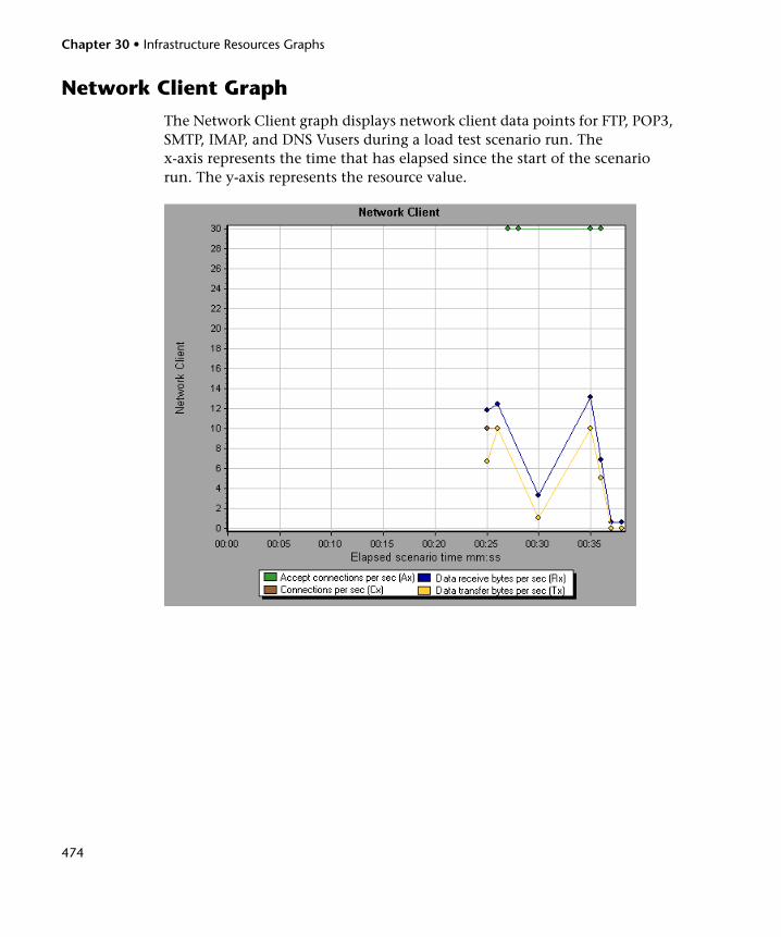
Chapter 30 • Infrastructure Resources Graphs
474
Network Client Graph
The Network Client graph displays network client data points for FTP, POP3, SMTP, IMAP, and DNS Vusers during a load test scenario run. The x-axis represents the time that has elapsed since the start of the scenario run. The y-axis represents the resource value.
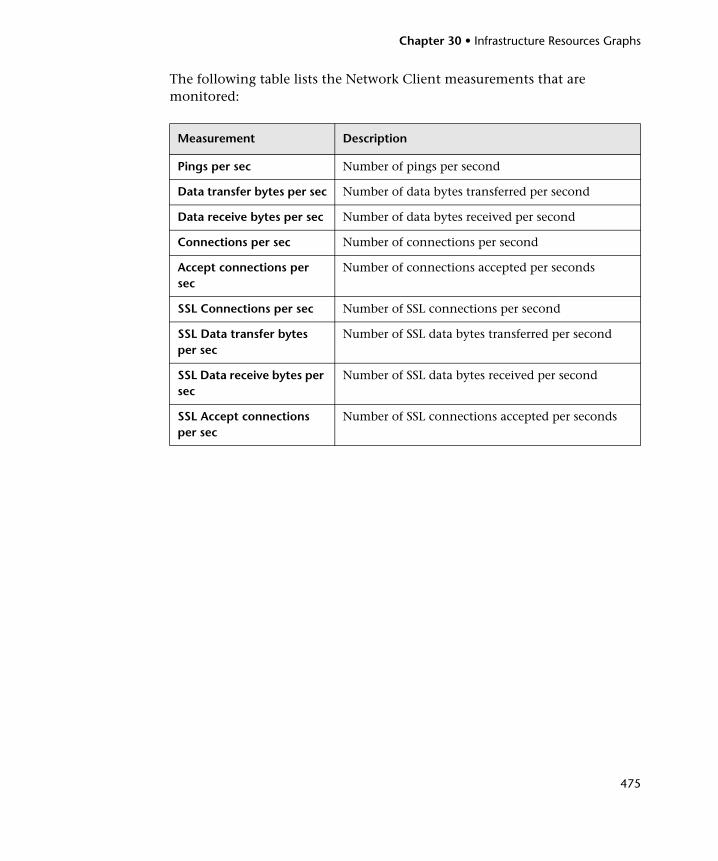
Chapter 30 • Infrastructure Resources Graphs
475
The following table lists the Network Client measurements that are monitored:
Measurement Description
Pings per sec Number of pings per second
Data transfer bytes per sec Number of data bytes transferred per second
Data receive bytes per sec Number of data bytes received per second
Connections per sec Number of connections per second
Accept connections per sec
Number of connections accepted per seconds
SSL Connections per sec Number of SSL connections per second
SSL Data transfer bytes per sec
Number of SSL data bytes transferred per second
SSL Data receive bytes per sec
Number of SSL data bytes received per second
SSL Accept connections per sec
Number of SSL connections accepted per seconds

Chapter 30 • Infrastructure Resources Graphs
476
Part III
Analysis Reports

478
479
31 Understanding Analysis Reports
After running a load test scenario, you can use the Analysis reports to analyze the performance of your application.
This chapter includes:
➤ About Analysis Reports on page 480
➤ Viewing Summary Reports on page 481
➤ SLA Reports on page 489
➤ Analyzing Transactions on page 491
➤ Creating HTML Reports on page 499
➤ Working with Transaction Reports on page 500
➤ Scenario Execution Report on page 503
➤ Failed Transaction Report on page 503
➤ Failed Vuser Report on page 504
➤ Data Point Report on page 504
➤ Detailed Transactions Reports on page 506
➤ Transaction Performance by Vuser Report on page 507
You can also create a report in Microsoft Word format. See Chapter 32, “Creating a Microsoft Word Report.”
Chapter 31 • Understanding Analysis Reports
480
About Analysis Reports
After running a load test scenario, you can view reports that summarize your system’s performance. Analysis provides the following reporting tools:
➤ Summary report
➤ SLA report
➤ Transaction Analysis reports
➤ HTML reports
➤ Transaction reports
The Summary report provides general information about the scenario run. You can access the Summary report at any time from the Session Explorer.
The SLA report provides an overview of the defined SLAs (Service Level Agreements) with succeeded or failed status.
The Transaction Analysis report provides a detailed analysis of a specific transaction over a specific time period.
You can instruct Analysis to create an HTML report. The HTML report contains a page for each open graph, the Summary report, the SLA report, and the Transaction Analysis report.
Transaction reports provide performance information about the transactions defined within the Vuser scripts. These reports give you a statistical breakdown of your results and allow you to print and export the data.
Note: Summary reports, SLA reports, and Transaction Analysis reports are not available when generating Cross Result graphs. For more information on Cross Result graphs, see Chapter 7, “Cross Result and Merged Graphs”.
Chapter 31 • Understanding Analysis Reports
481
Viewing Summary Reports
The Summary report provides general information about load test scenario execution. This report is always available from the Session Explorer or as a tab in the Analysis window.
The Summary report lists statistics about the scenario run and provides links to the following graphs: Running Vusers, Throughput, Hits Per Second, HTTP Responses per Second, Transaction Summary, and Average Transaction Response Time.
The appearance of the Summary report and the information displayed, will vary depending on whether an SLA (Service Level Agreement) was defined.
An SLA defines goals for the scenario. LoadRunner measures these goals during the scenario run and analyzes them in the Summary report. For more information on defining an SLA, see Chapter 8, “Defining Service Level Agreements.”
Summary reports are also provided for Cross Result graphs. For more information about Cross Result graphs, see “Cross Result Graphs” on page 128.
This section includes:
➤ “Summary Report With No SLA” below
➤ “Summary Report With SLA” on page 484
➤ “Summary Reports for Cross Result Graphs” on page 488
Summary Report With No SLAThe Summary report where no SLA was defined contains the following sections.
➤ Scenario Details
➤ Statistics Summary
➤ Scenario Behavior Over Time
➤ Transaction Summary
➤ HTTP Responses Summary
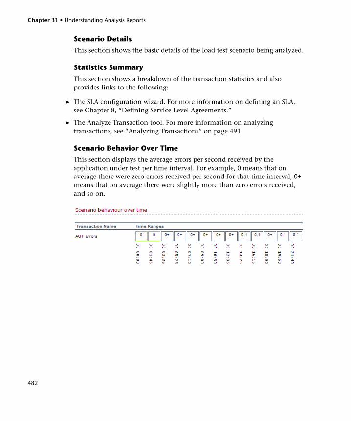
Chapter 31 • Understanding Analysis Reports
482
Scenario Details
This section shows the basic details of the load test scenario being analyzed.
Statistics Summary
This section shows a breakdown of the transaction statistics and also provides links to the following:
➤ The SLA configuration wizard. For more information on defining an SLA, see Chapter 8, “Defining Service Level Agreements.”
➤ The Analyze Transaction tool. For more information on analyzing transactions, see “Analyzing Transactions” on page 491
Scenario Behavior Over Time
This section displays the average errors per second received by the application under test per time interval. For example, 0 means that on average there were zero errors received per second for that time interval, 0+ means that on average there were slightly more than zero errors received, and so on.
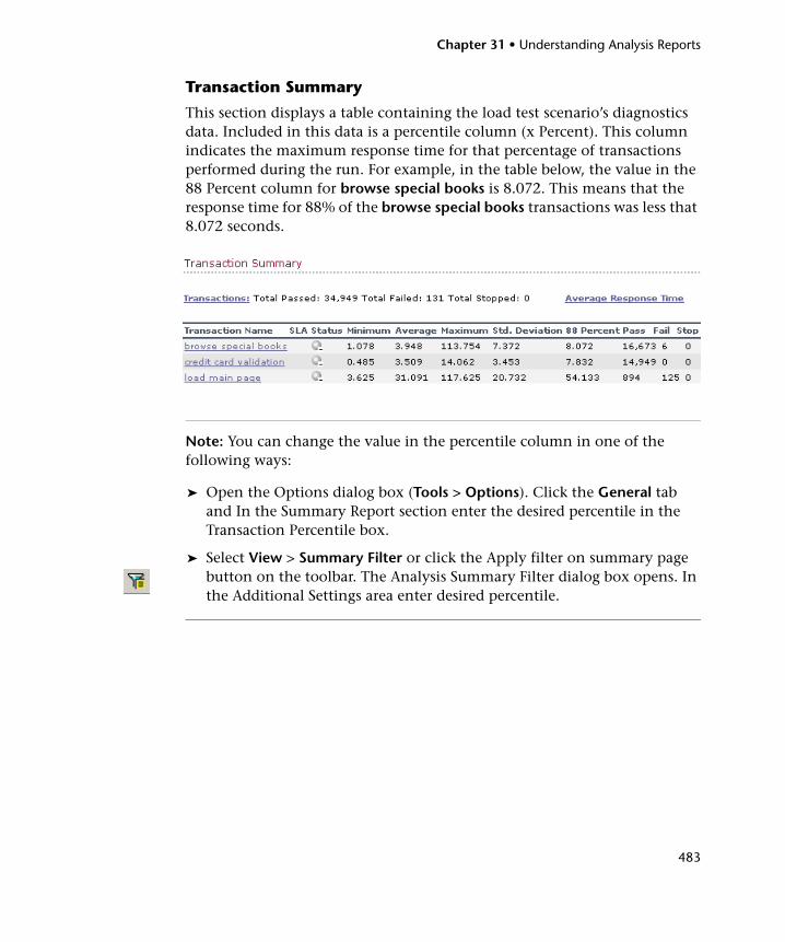
Chapter 31 • Understanding Analysis Reports
483
Transaction Summary
This section displays a table containing the load test scenario’s diagnostics data. Included in this data is a percentile column (x Percent). This column indicates the maximum response time for that percentage of transactions performed during the run. For example, in the table below, the value in the 88 Percent column for browse special books is 8.072. This means that the response time for 88% of the browse special books transactions was less that 8.072 seconds.
Note: You can change the value in the percentile column in one of the following ways:
➤ Open the Options dialog box (Tools > Options). Click the General tab and In the Summary Report section enter the desired percentile in the Transaction Percentile box.
➤ Select View > Summary Filter or click the Apply filter on summary page button on the toolbar. The Analysis Summary Filter dialog box opens. In the Additional Settings area enter desired percentile.
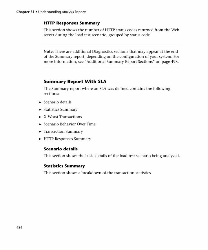
Chapter 31 • Understanding Analysis Reports
484
HTTP Responses Summary
This section shows the number of HTTP status codes returned from the Web server during the load test scenario, grouped by status code.
Note: There are additional Diagnostics sections that may appear at the end of the Summary report, depending on the configuration of your system. For more information, see “Additional Summary Report Sections” on page 498.
Summary Report With SLAThe Summary report where an SLA was defined contains the following sections:
➤ Scenario details
➤ Statistics Summary
➤ X Worst Transactions
➤ Scenario Behavior Over Time
➤ Transaction Summary
➤ HTTP Responses Summary
Scenario details
This section shows the basic details of the load test scenario being analyzed.
Statistics Summary
This section shows a breakdown of the transaction statistics.
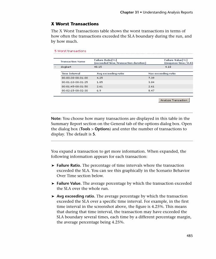
Chapter 31 • Understanding Analysis Reports
485
X Worst Transactions
The X Worst Transactions table shows the worst transactions in terms of how often the transactions exceeded the SLA boundary during the run, and by how much.
Note: You choose how many transactions are displayed in this table in the Summary Report section on the General tab of the options dialog box. Open the dialog box (Tools > Options) and enter the number of transactions to display. The default is 5.
You expand a transaction to get more information. When expanded, the following information appears for each transaction:
➤ Failure Ratio. The percentage of time intervals where the transaction exceeded the SLA. You can see this graphically in the Scenario Behavior Over Time section below.
➤ Failure Value. The average percentage by which the transaction exceeded the SLA over the whole run.
➤ Avg exceeding ratio. The average percentage by which the transaction exceeded the SLA over a specific time interval. For example, in the first time interval in the screenshot above, the figure is 4.25%. This means that during that time interval, the transaction may have exceeded the SLA boundary several times, each time by a different percentage margin, the average percentage being 4.25%.
Chapter 31 • Understanding Analysis Reports
486
➤ Max exceeding ratio. The highest percentage by which the transaction exceeded the SLA over a specific time interval. For example, using the same time interval as above, the transaction may have exceeded the SLA several times, each time by a different percentage margin. The highest percentage being 7.39%
Analysis allows you to analyze a specific transaction in more detail. You open the Analyze Transaction tool from this section by clicking the Analyze Transaction button. For more information on Transaction Analysis Reports, see “Analyzing Transactions” on page 491.
Scenario Behavior Over Time
This section shows how each transaction performed in terms of the SLA over time intervals. The green squares show time intervals where the transaction performed within the SLA boundary. Red squares show time intervals where the transaction failed and grey squares show where no relevant SLA was defined.
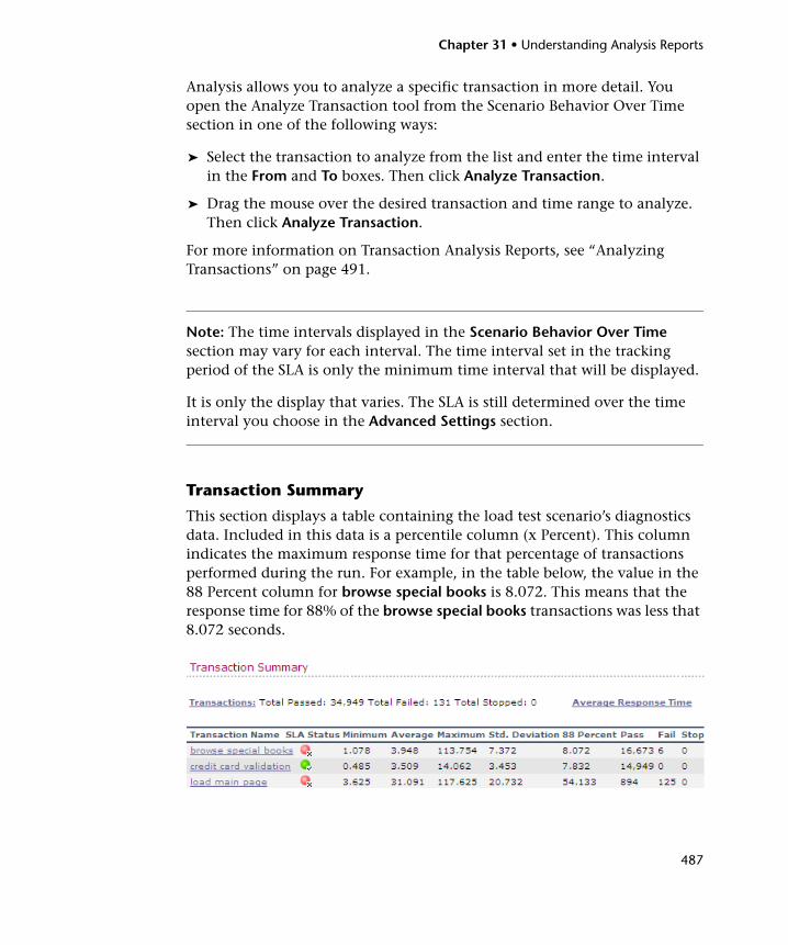
Chapter 31 • Understanding Analysis Reports
487
Analysis allows you to analyze a specific transaction in more detail. You open the Analyze Transaction tool from the Scenario Behavior Over Time section in one of the following ways:
➤ Select the transaction to analyze from the list and enter the time interval in the From and To boxes. Then click Analyze Transaction.
➤ Drag the mouse over the desired transaction and time range to analyze. Then click Analyze Transaction.
For more information on Transaction Analysis Reports, see “Analyzing Transactions” on page 491.
Note: The time intervals displayed in the Scenario Behavior Over Time section may vary for each interval. The time interval set in the tracking period of the SLA is only the minimum time interval that will be displayed.
It is only the display that varies. The SLA is still determined over the time interval you choose in the Advanced Settings section.
Transaction Summary
This section displays a table containing the load test scenario’s diagnostics data. Included in this data is a percentile column (x Percent). This column indicates the maximum response time for that percentage of transactions performed during the run. For example, in the table below, the value in the 88 Percent column for browse special books is 8.072. This means that the response time for 88% of the browse special books transactions was less that 8.072 seconds.
Chapter 31 • Understanding Analysis Reports
488
Note: You can change the value in the percentile column in the Summary Report section of the General tab of the Options dialog box. Open the dialog box (Tools > Options) and enter the desired percentage.
Alternatively, you can also change the value in the Summary Filter (View > Summary Filter)
HTTP Responses Summary
This section shows the number of HTTP status codes returned from the Web server during the load test scenario, grouped by status code.
Note: There are additional Diagnostics sections that may appear at the end of the Summary report, depending on the configuration of your system. For more information, see “Additional Summary Report Sections” on page 498.
Summary Reports for Cross Result GraphsThe Summary report for Cross Result graphs displays summary information for the scenarios that you are comparing. The information is displayed in a way that enables you to compare data from the different scenarios.
The Summary report for Cross Result graphs includes the same type of information as the regular Summary report except for the following:
➤ SLA information
➤ Diagnostics information
➤ Scenario behavior over time
In the Transaction Summary section of the report, you can export the table to a CSV file by clicking the Save this table to a CSV file link.
Chapter 31 • Understanding Analysis Reports
489
SLA Reports
An SLA (Service Level Agreement) defines goals for the load test scenario. LoadRunner measures these goals during the scenario run and analyzes them in the Summary report. The SLA Report shows the succeeded or failed status of all SLAs that were defined for the scenario run. For more information on defining an SLA, see Chapter 8, “Defining Service Level Agreements.”
Note: Analysis data (for example, transactions) that has been excluded by the Summary Filter will not be available for analysis in the SLA report. For more information on filtering, see “Applying Filter and Sort Criteria to Graphs” on page 81
You create the SLA Report in one of the following ways:
➤ Select Reports > Analyze SLA. The SLA report opens.
➤ Right-Click the Summary pane and select Analyze SLA from the right-click menu. The SLA report opens.
➤ Click on any SLA status indicator that appears in the Summary Report.
Once the report has been created, it can be accessed at any time from the Session Explorer.
Depending on the measurements that you are evaluating, the SLA report displays the SLA statuses in one of the following ways:
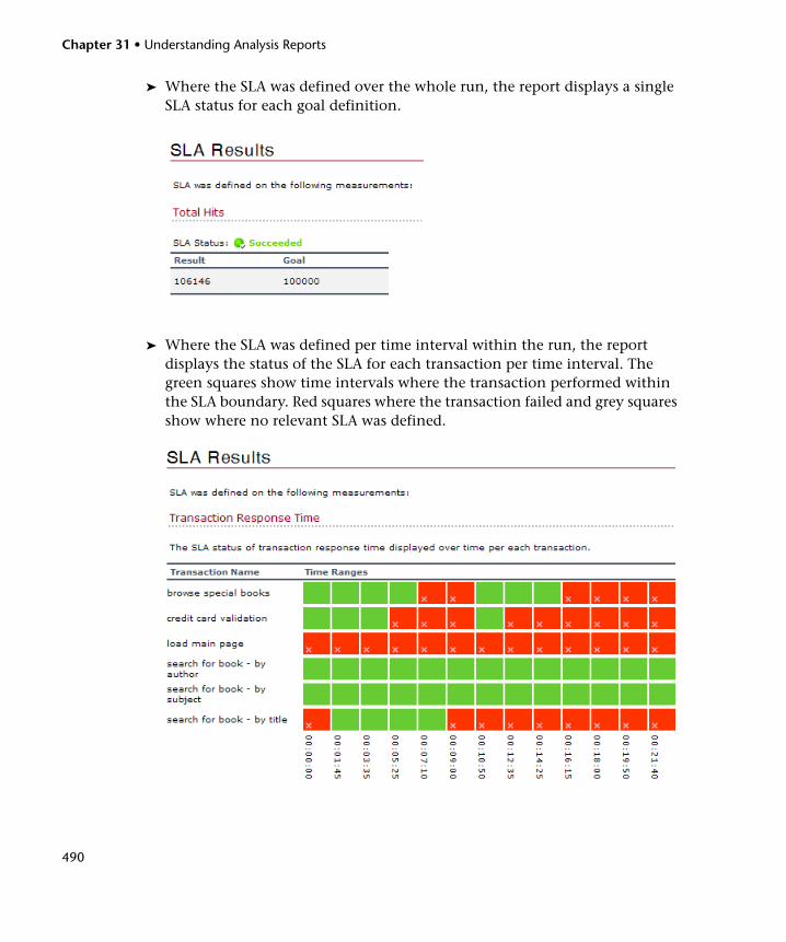
Chapter 31 • Understanding Analysis Reports
490
➤ Where the SLA was defined over the whole run, the report displays a single SLA status for each goal definition.
➤ Where the SLA was defined per time interval within the run, the report displays the status of the SLA for each transaction per time interval. The green squares show time intervals where the transaction performed within the SLA boundary. Red squares where the transaction failed and grey squares show where no relevant SLA was defined.
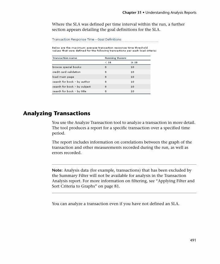
Chapter 31 • Understanding Analysis Reports
491
Where the SLA was defined per time interval within the run, a further section appears detailing the goal definitions for the SLA.
Analyzing Transactions
You use the Analyze Transaction tool to analyze a transaction in more detail. The tool produces a report for a specific transaction over a specified time period.
The report includes information on correlations between the graph of the transaction and other measurements recorded during the run, as well as errors recorded.
Note: Analysis data (for example, transactions) that has been excluded by the Summary Filter will not be available for analysis in the Transaction Analysis report. For more information on filtering, see “Applying Filter and Sort Criteria to Graphs” on page 81.
You can analyze a transaction even if you have not defined an SLA.
Chapter 31 • Understanding Analysis Reports
492
To open the Analyze Transaction tool:
You open the tool in one of the following ways:
➤ Select Reports > Analyze Transaction. The Analyze Transaction dialog box opens.
➤ Right-Click the Summary Report pane and select Analyze Transaction from the right-click menu. The Analyze Transaction dialog box opens.
➤ Click the Analyze Transaction button on the toolbar. The Analyze Transaction dialog box opens.
➤ Where an SLA has been defined, click on the Analyze Transaction button that appears by the X Worst Transactions section or the Scenario Behavior Over Time section. In these cases, Analysis opens the Transaction Analysis Report directly using the last used settings, and not the Analyze Transaction dialog box.
➤ Where an SLA has not been defined, click the Analyze Transaction tool link in the Statistics Summary section. The Analyze Transaction dialog box opens.
➤ Generate the report automatically using Analysis Templates. To do this, select Tools > Templates > Apply/Edit Template. Select Automatically analyze the top problematic transactions and click Apply Template. For more information about working with templates, see “Using Templates” on page 76.
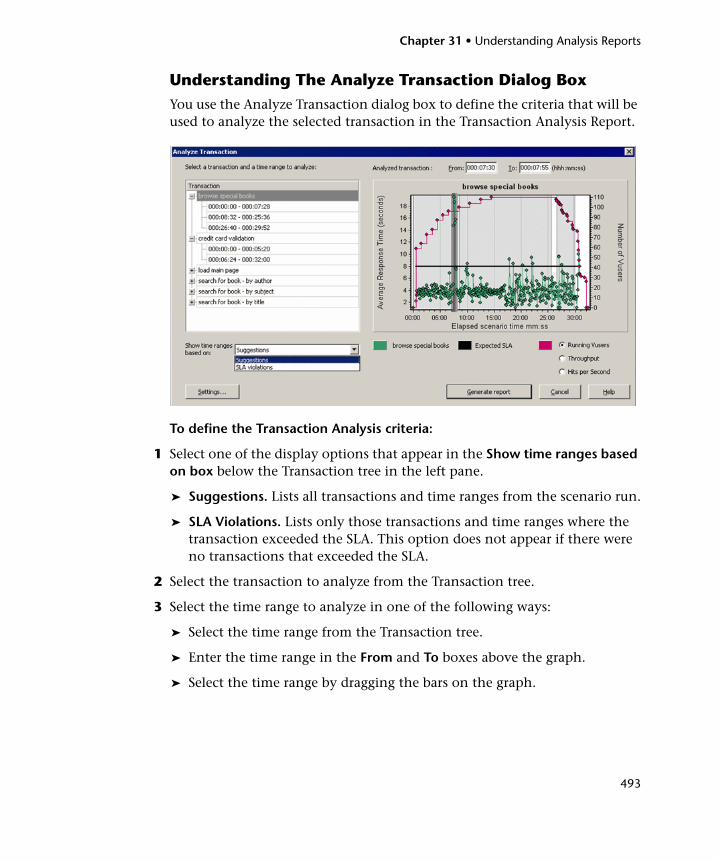
Chapter 31 • Understanding Analysis Reports
493
Understanding The Analyze Transaction Dialog BoxYou use the Analyze Transaction dialog box to define the criteria that will be used to analyze the selected transaction in the Transaction Analysis Report.
To define the Transaction Analysis criteria:
1 Select one of the display options that appear in the Show time ranges based on box below the Transaction tree in the left pane.
➤ Suggestions. Lists all transactions and time ranges from the scenario run.
➤ SLA Violations. Lists only those transactions and time ranges where the transaction exceeded the SLA. This option does not appear if there were no transactions that exceeded the SLA.
2 Select the transaction to analyze from the Transaction tree.
3 Select the time range to analyze in one of the following ways:
➤ Select the time range from the Transaction tree.
➤ Enter the time range in the From and To boxes above the graph.
➤ Select the time range by dragging the bars on the graph.
Chapter 31 • Understanding Analysis Reports
494
4 Select one of the display options from Running Vusers, Throughput and Hits per Second from the radio buttons under the graph. The option you select is displayed on the graph and will appear on the snapshot of the graph that appears on the Transaction Analysis Report. Note that your choice only affects the display of the graph and not the calculation for correlations.
5 Click Settings to define the Analyze Transaction settings in the Analyze Transaction Settings dialog box. For more information, see “Understanding the Analyze Transaction Settings” below
Note: You can also define the Analyze Transaction settings in the Analyze Transaction Settings tab of the Options dialog box (Tools > Options).
6 Click Generate report. The Transaction Analysis Report opens. Once the report has been created, you can access it at any time from the Session Explorer.
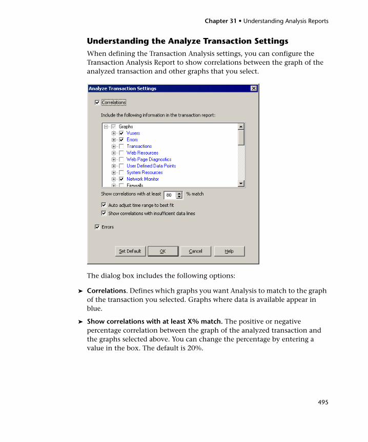
Chapter 31 • Understanding Analysis Reports
495
Understanding the Analyze Transaction SettingsWhen defining the Transaction Analysis settings, you can configure the Transaction Analysis Report to show correlations between the graph of the analyzed transaction and other graphs that you select.
The dialog box includes the following options:
➤ Correlations. Defines which graphs you want Analysis to match to the graph of the transaction you selected. Graphs where data is available appear in blue.
➤ Show correlations with at least X% match. The positive or negative percentage correlation between the graph of the analyzed transaction and the graphs selected above. You can change the percentage by entering a value in the box. The default is 20%.
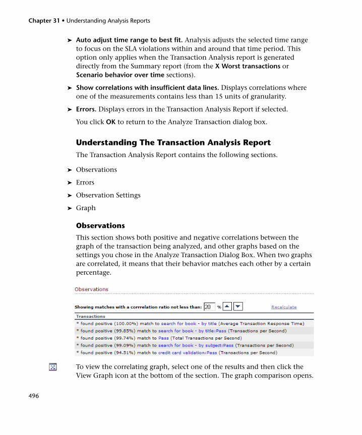
Chapter 31 • Understanding Analysis Reports
496
➤ Auto adjust time range to best fit. Analysis adjusts the selected time range to focus on the SLA violations within and around that time period. This option only applies when the Transaction Analysis report is generated directly from the Summary report (from the X Worst transactions or Scenario behavior over time sections).
➤ Show correlations with insufficient data lines. Displays correlations where one of the measurements contains less than 15 units of granularity.
➤ Errors. Displays errors in the Transaction Analysis Report if selected.
You click OK to return to the Analyze Transaction dialog box.
Understanding The Transaction Analysis ReportThe Transaction Analysis Report contains the following sections.
➤ Observations
➤ Errors
➤ Observation Settings
➤ Graph
Observations
This section shows both positive and negative correlations between the graph of the transaction being analyzed, and other graphs based on the settings you chose in the Analyze Transaction Dialog Box. When two graphs are correlated, it means that their behavior matches each other by a certain percentage.
To view the correlating graph, select one of the results and then click the View Graph icon at the bottom of the section. The graph comparison opens.
Chapter 31 • Understanding Analysis Reports
497
You can return to the Transaction Analysis Report from the graph comparison at anytime by clicking the Back to <transaction name> icon on the toolbar.
Note: The correlations are automatically calculated according to a default ratio of 20%. You can adjust this ratio by clicking the arrows next to the percentage. Then click Recalculate.
Errors
This section is divided into two sub-sections.
➤ Application Under Test errors. Shows errors that occurred during the transaction that were direct results of Vuser activity.
➤ All errors. Shows Application Under Test errors as well as errors that were not related to Vuser activity, and which affected your system and not the application under test.
Observation Settings
This section displays a summary of the settings that were selected in the Advanced Settings section of the Analyze Transaction dialog box.
Graph
The Graph section displays a snapshot of selected transaction and time range for analysis merged with the display option you selected (Running Vusers, Throughput, or Hits per Second). Note that it is only a snapshot and can not be manipulated like normal graphs.
Chapter 31 • Understanding Analysis Reports
498
Additional Summary Report SectionsThere are additional Diagnostics sections that may appear at the end of the Summary Report, depending on the configuration of your system.
Viewing Diagnostics from the Summary Report
The Summary report for SAP Diagnostics, J2EE /.NET Diagnostics, and Siebel Diagnostics provides a usage chart that links to and displays each individual transaction’s Web, application, and database layers, and provides the total usage time for each transaction. You can click a layer on which you want to perform transaction breakdown to open the breakdown graph for the selected transaction.
The Summary reports for the various diagnostics environments are discussed in detail in the following sections:
➤ “Viewing the Siebel Usage Section of the Summary Report” on page 526
➤ “Viewing the SAP Diagnostics in the Summary Report” on page 583
➤ “Viewing J2EE & .NET Diagnostics in the Summary Report” on page 607
Exporting the Summary Report to Excel
You can save the Summary report to an Excel file by selecting View > Export Summary to Excel.
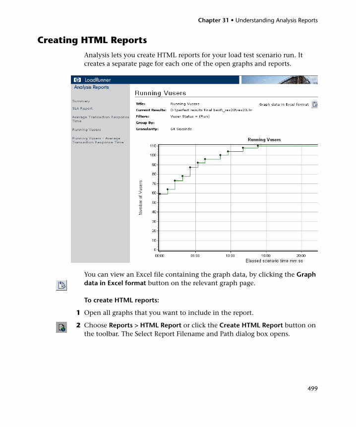
Chapter 31 • Understanding Analysis Reports
499
Creating HTML Reports
Analysis lets you create HTML reports for your load test scenario run. It creates a separate page for each one of the open graphs and reports.
You can view an Excel file containing the graph data, by clicking the Graph data in Excel format button on the relevant graph page.
To create HTML reports:
1 Open all graphs that you want to include in the report.
2 Choose Reports > HTML Report or click the Create HTML Report button on the toolbar. The Select Report Filename and Path dialog box opens.
Chapter 31 • Understanding Analysis Reports
500
3 Specify a path and file name for the HTML report and click Save. Analysis saves a Summary report which has the same name as the file in the selected folder. The rest of the graphs are saved in a folder with the same name as the Summary report’s file name. When you create an HTML report, Analysis opens your default browser and displays the Summary report.
4 To view an HTML report for one of the graphs, click its link in the left frame.
5 To copy the HTML reports to another location, be sure to copy the filename and the folder with the same name. For example, if you named your HTML report test1, copy test1.html and the folder test1 to the desired location.
Working with Transaction Reports
LoadRunner’s Transaction reports are divided into the following categories:
➤ Activity
➤ Performance
Activity reports provide information about the number of Vusers and the number of transactions executed during the load test scenario run. The available Activity reports are Scenario Execution, Failed Transaction, and Failed Vusers.
Performance reports analyze Vuser performance and transaction times. The available Performance reports are Data Point, Detailed Transaction, and Transaction Performance by Vuser.
In order to view a report, you must generate it from the Analysis window. Analysis reports are displayed in a Report Viewer. You can print, save, or export the data using the viewer.
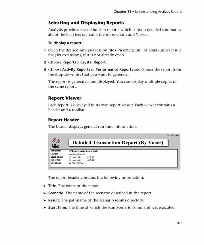
Chapter 31 • Understanding Analysis Reports
501
Selecting and Displaying ReportsAnalysis provides several built-in reports which contain detailed summaries about the load test scenario, the transactions and Vusers.
To display a report:
1 Open the desired Analysis session file (.lra extension), or LoadRunner result file (.lrr extension), if it is not already open.
2 Choose Reports > Crystal Report.
3 Choose Activity Reports or Performance Reports and choose the report from the drop-down list that you want to generate.
The report is generated and displayed. You can display multiple copies of the same report.
Report ViewerEach report is displayed in its own report viewer. Each viewer contains a header and a toolbar.
Report Header
The header displays general run time information.
The report header contains the following information:
➤ Title. The name of the report.
➤ Scenario. The name of the scenario described in the report.
➤ Result. The pathname of the scenario results directory.
➤ Start time. The time at which the Run Scenario command was executed.
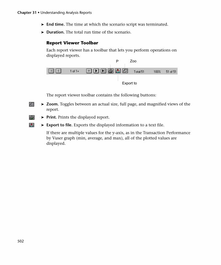
Chapter 31 • Understanding Analysis Reports
502
➤ End time. The time at which the scenario script was terminated.
➤ Duration. The total run time of the scenario.
Report Viewer Toolbar
Each report viewer has a toolbar that lets you perform operations on displayed reports.
The report viewer toolbar contains the following buttons:
➤ Zoom. Toggles between an actual size, full page, and magnified views of the report.
➤ Print. Prints the displayed report.
➤ Export to file. Exports the displayed information to a text file.
If there are multiple values for the y-axis, as in the Transaction Performance by Vuser graph (min, average, and max), all of the plotted values are displayed.
Zoo
Export to
P
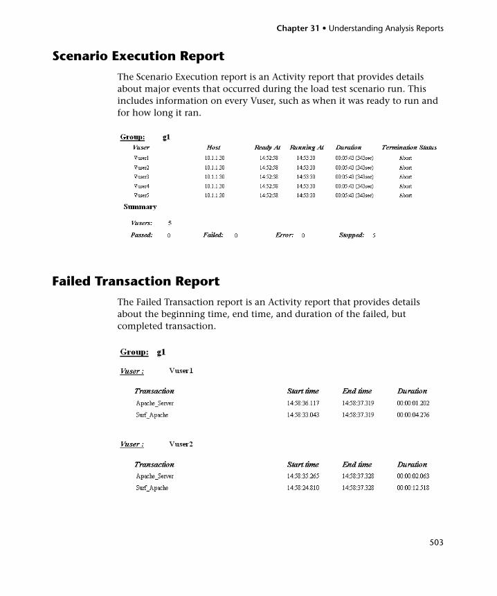
Chapter 31 • Understanding Analysis Reports
503
Scenario Execution Report
The Scenario Execution report is an Activity report that provides details about major events that occurred during the load test scenario run. This includes information on every Vuser, such as when it was ready to run and for how long it ran.
Failed Transaction Report
The Failed Transaction report is an Activity report that provides details about the beginning time, end time, and duration of the failed, but completed transaction.
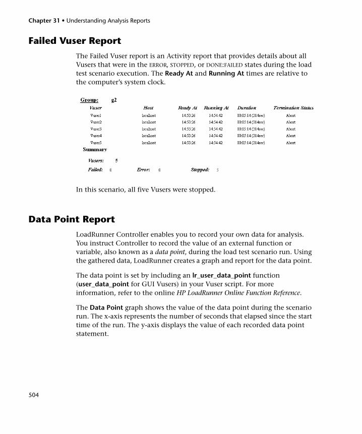
Chapter 31 • Understanding Analysis Reports
504
Failed Vuser Report
The Failed Vuser report is an Activity report that provides details about all Vusers that were in the ERROR, STOPPED, or DONE:FAILED states during the load test scenario execution. The Ready At and Running At times are relative to the computer’s system clock.
In this scenario, all five Vusers were stopped.
Data Point Report
LoadRunner Controller enables you to record your own data for analysis. You instruct Controller to record the value of an external function or variable, also known as a data point, during the load test scenario run. Using the gathered data, LoadRunner creates a graph and report for the data point.
The data point is set by including an lr_user_data_point function (user_data_point for GUI Vusers) in your Vuser script. For more information, refer to the online HP LoadRunner Online Function Reference.
The Data Point graph shows the value of the data point during the scenario run. The x-axis represents the number of seconds that elapsed since the start time of the run. The y-axis displays the value of each recorded data point statement.

Chapter 31 • Understanding Analysis Reports
505
The Data Point report is a Performance report that lists the name of the data point, its value, and the time its value was recorded. The values are displayed for each Group and Vuser.
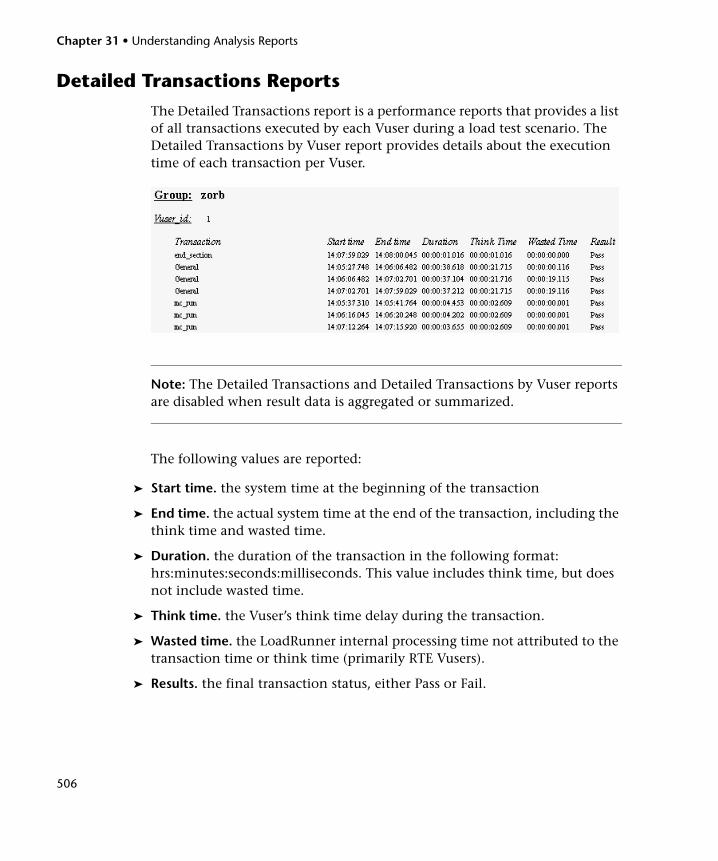
Chapter 31 • Understanding Analysis Reports
506
Detailed Transactions Reports
The Detailed Transactions report is a performance reports that provides a list of all transactions executed by each Vuser during a load test scenario. The Detailed Transactions by Vuser report provides details about the execution time of each transaction per Vuser.
Note: The Detailed Transactions and Detailed Transactions by Vuser reports are disabled when result data is aggregated or summarized.
The following values are reported:
➤ Start time. the system time at the beginning of the transaction
➤ End time. the actual system time at the end of the transaction, including the think time and wasted time.
➤ Duration. the duration of the transaction in the following format: hrs:minutes:seconds:milliseconds. This value includes think time, but does not include wasted time.
➤ Think time. the Vuser’s think time delay during the transaction.
➤ Wasted time. the LoadRunner internal processing time not attributed to the transaction time or think time (primarily RTE Vusers).
➤ Results. the final transaction status, either Pass or Fail.
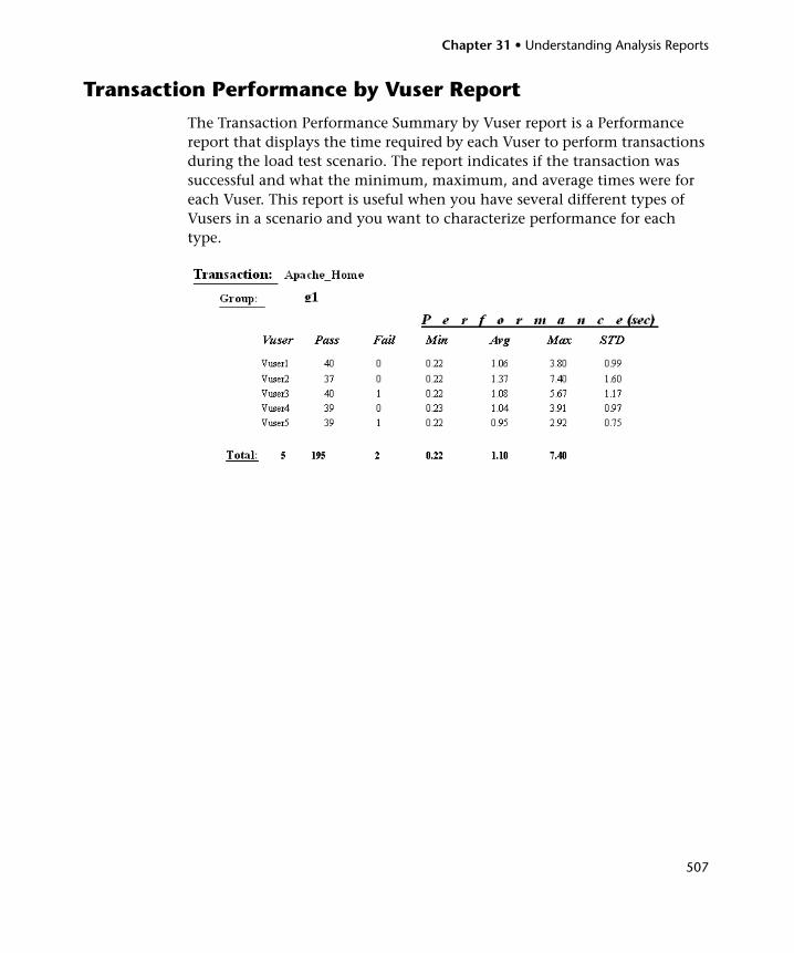
Chapter 31 • Understanding Analysis Reports
507
Transaction Performance by Vuser Report
The Transaction Performance Summary by Vuser report is a Performance report that displays the time required by each Vuser to perform transactions during the load test scenario. The report indicates if the transaction was successful and what the minimum, maximum, and average times were for each Vuser. This report is useful when you have several different types of Vusers in a scenario and you want to characterize performance for each type.

Chapter 31 • Understanding Analysis Reports
508
509
32 Creating a Microsoft Word Report
You can create a report as a Microsoft Word document.
This chapter includes:
➤ About the Microsoft Word Report on page 509
➤ Creating Microsoft Word Reports on page 510
About the Microsoft Word Report
You can use the Word report generation tool to automatically summarize and display the test’s significant data in graphical and tabular format and to display and describe all graphs and reports in the current Analysis session.
You can also choose to include the script from VuGen to display thumbnail images of the business process.
The appearance of the Summary report and the information displayed, will vary depending on whether an SLA (Service Level Agreement) was defined. For more information on Summary reports, see “Viewing Summary Reports” on page 481.
If an SLA was defined and a report was generated (Reports > Analyze SLA), then the Word report will also include the SLA report. For more information on SLA reports, see “SLA Reports” on page 489.
Other features of the report include the automatic inclusion of an overview of the load test scenario configuration, and an executive summary.
The report is structured into logical and intuitive sections with a table of contents and various appendixes.
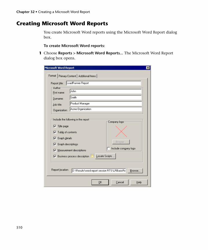
Chapter 32 • Creating a Microsoft Word Report
510
Creating Microsoft Word Reports
You create Microsoft Word reports using the Microsoft Word Report dialog box.
To create Microsoft Word reports:
1 Choose Reports > Microsoft Word Reports... The Microsoft Word Report dialog box opens.
Chapter 32 • Creating a Microsoft Word Report
511
2 Enter the Microsoft Word report options as described in the following sections:
➤ “Understanding the Microsoft Word Report Dialog Box-Format Tab” on page 511.
➤ “Understanding the Microsoft Word Report Dialog Box-Primary Content Tab” on page 515.
➤ “Understanding the Microsoft Word Report Dialog Box-Additional Items Tab” on page 517.
3 Click OK. The report generation process may take a few minutes.
When completed, Analysis launches the Microsoft Word application containing the report. The file is saved to the location specified in the Report Location box of the Format tab.
Understanding the Microsoft Word Report Dialog Box-Format TabYou use the Format tab to add custom title and author information to the Word report, as well as to include additional pages and descriptive comments.
➤ Report title. Enter a name for the report. This will be displayed on the report’s title page.
➤ Author. Enter the author details. This will be displayed on the report’s title page.
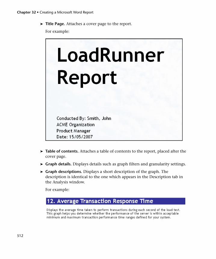
Chapter 32 • Creating a Microsoft Word Report
512
➤ Title Page. Attaches a cover page to the report.
For example:
➤ Table of contents. Attaches a table of contents to the report, placed after the cover page.
➤ Graph details. Displays details such as graph filters and granularity settings.
➤ Graph descriptions. Displays a short description of the graph. The description is identical to the one which appears in the Description tab in the Analysis window.
For example:
Chapter 32 • Creating a Microsoft Word Report
513
➤ Measurement descriptions. Attaches descriptions of each type of monitor measurement in the report appendix.
➤ Business process description. Inserts script details into the report. For more information on this option, see “Viewing Script Details” on page 513
➤ Report location. Enter the path to the Microsoft Word report.
➤ Include Company logo. Includes a logo (.bmp format) in the report.
Viewing Script Details
This option inserts script details into the report and allows you to view thumbnail images of the business process steps.
The following script types support thumbnails: AJAX (Click and Script), Citrix_ICA, Oracle Web Applications 11i, People Soft Enterprise, People Soft-Tuxedo, Web (HTTP/HTML), SAP-Web, SAPGUI, Sap (Click and Script), Web (Click and Script).
The option is disabled when the script cannot be located or when there is a problem with the script. For example, if the script does not support thumbnails.
When then the option will be disabled, a triangle will appear. If you hold the mouse over the option, a tooltip will display the reason for the problem. You hold the mouse over the triangle to display a tooltip with a suggested solution.
To locate a valid script, click the Locate Scripts button to select a script from a different location.
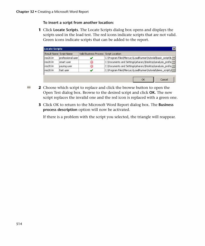
Chapter 32 • Creating a Microsoft Word Report
514
To insert a script from another location:
1 Click Locate Scripts. The Locate Scripts dialog box opens and displays the scripts used in the load test. The red icons indicate scripts that are not valid. Green icons indicate scripts that can be added to the report.
2 Choose which script to replace and click the browse button to open the Open Test dialog box. Browse to the desired script and click OK. The new script replaces the invalid one and the red icon is replaced with a green one.
3 Click OK to return to the Microsoft Word Report dialog box. The Business process description option will now be activated.
If there is a problem with the script you selected, the triangle will reappear.
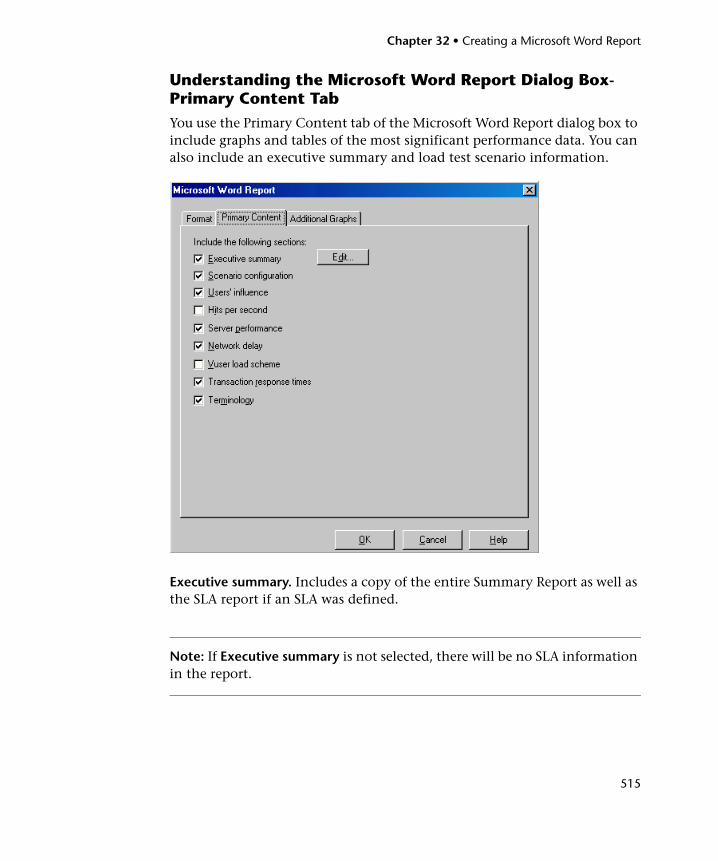
Chapter 32 • Creating a Microsoft Word Report
515
Understanding the Microsoft Word Report Dialog Box-Primary Content TabYou use the Primary Content tab of the Microsoft Word Report dialog box to include graphs and tables of the most significant performance data. You can also include an executive summary and load test scenario information.
Executive summary. Includes a copy of the entire Summary Report as well as the SLA report if an SLA was defined.
Note: If Executive summary is not selected, there will be no SLA information in the report.
Chapter 32 • Creating a Microsoft Word Report
516
The summary also includes your own high-level summary or abstract of the LoadRunner test, suitable for senior management.
To create the Executive summary, click Edit and enter the text in the Executive Summary dialog box. An executive summary typically compares performance data with business goals, states significant findings and conclusions in non-technical language, and suggests recommendations.
Chapter 32 • Creating a Microsoft Word Report
517
➤ Scenario configuration. Gives the basic schema of the test, including the name of result files, Controller scheduler information, scripts, and Run Time Settings.
➤ Users’ influence. A graph that helps you view the general impact of Vuser load on performance time. It is most useful when analyzing a load test which is run with a gradual load.
➤ Hits per second. Applicable to Web tests. Displays the number of hits made on the Web server by Vusers during each second of the load test. It helps you evaluate the amount of load Vusers generate, in terms of the number of hits.
➤ Server performance. A graph that displays a summary of resources utilized on the servers.
➤ Network delay. Displays the delays for the complete network path between machines.
➤ Vuser load scheme. Displays the number of Vusers that executed Vuser scripts, and their status, during each second of a load test. This graph is useful for determining the Vuser load on your server at any given moment.
➤ Transaction response times. Displays the average time taken to perform transactions during each second of the load test. This graph helps you determine whether the performance of the server is within acceptable minimum and maximum transaction performance time ranges defined for your system.
➤ Terminology. Displays an explanation of special terms used in the report.
Understanding the Microsoft Word Report Dialog Box-Additional Items TabYou use the Additional Items tab of the Microsoft Word Report dialog box to include graphs and Transaction Analysis Reports in the Word report. The graphs and Transaction Analysis Reports that were generated in the current Analysis session are listed in the dialog box. You can also add other
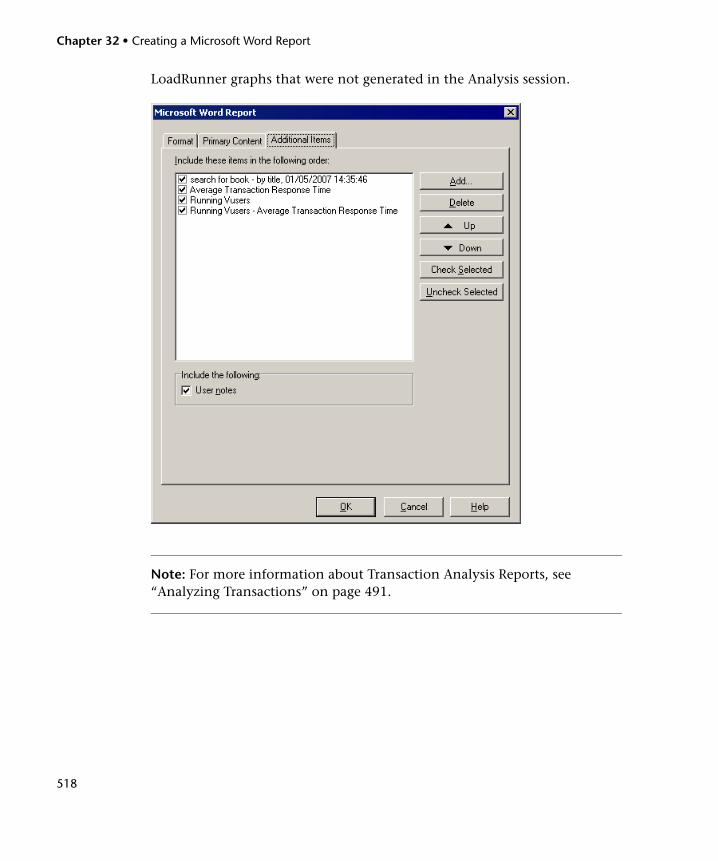
Chapter 32 • Creating a Microsoft Word Report
518
LoadRunner graphs that were not generated in the Analysis session.
Note: For more information about Transaction Analysis Reports, see “Analyzing Transactions” on page 491.
Chapter 32 • Creating a Microsoft Word Report
519
➤ Include the following: User notes. Select this to include text you entered for the graph in the Analysis User Notes window.
➤ Add. Opens the Open a New Graph dialog box to enable you to add other graphs not yet generated in the Analysis session. After selecting the graph, it will be generated and added to the Word Report. For more information, see “Accessing and Opening Graphs and Reports” on page 30.
➤ Delete. Deletes a selected graph from the list.
➤ Up/Down. Changes the order in which the graph is displayed in the Microsoft Word report.
➤ Check Selected. Selects the current report in the Include the following box.
➤ Uncheck Selected. Clears the selection of the current report in the Include the following box.

Chapter 32 • Creating a Microsoft Word Report
520

Part IV
Working with Diagnostics

522

523
33 Siebel Diagnostics Graphs
After a load test scenario run, you use the Siebel Diagnostics graphs to analyze Siebel server performance.
Note: Siebel DB Diagnostics graphs provide you with performance information for SQL statements generated by transactions on the Siebel system. For more information, see Chapter 34, “Siebel DB Diagnostics Graphs.”
This chapter includes:
➤ About Siebel Diagnostics Graphs on page 524
➤ Enabling Siebel Diagnostics on page 525
➤ Viewing the Siebel Usage Section of the Summary Report on page 526
➤ Viewing Siebel Diagnostics Data on page 528
➤ Available Siebel Diagnostics Graphs on page 540
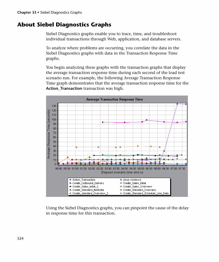
Chapter 33 • Siebel Diagnostics Graphs
524
About Siebel Diagnostics Graphs
Siebel Diagnostics graphs enable you to trace, time, and troubleshoot individual transactions through Web, application, and database servers.
To analyze where problems are occurring, you correlate the data in the Siebel Diagnostics graphs with data in the Transaction Response Time graphs.
You begin analyzing these graphs with the transaction graphs that display the average transaction response time during each second of the load test scenario run. For example, the following Average Transaction Response Time graph demonstrates that the average transaction response time for the Action_Transaction transaction was high.
Using the Siebel Diagnostics graphs, you can pinpoint the cause of the delay in response time for this transaction.
Chapter 33 • Siebel Diagnostics Graphs
525
Alternatively, you can use the Summary Report to view individual transactions broken down into Web, application, and database layers, and the total usage time for each transaction. For more information, see “Viewing the Siebel Usage Section of the Summary Report” on page 526.
Note: A measurement that is broken down in the Average Transaction Response Time graph will be different from the same measurement broken down in the Siebel Diagnostics graph. This is because the Average Transaction Response Time graph displays the average transaction response time, whereas the Siebel Diagnostics graph displays the average time per transaction event (sum of Siebel Area response time).
Enabling Siebel Diagnostics
To generate Siebel diagnostics data, you must first install the ERP/CRM Mediator (Mediator). For information on installing the Mediator, refer to the HP LoadRunner Installation Guide.
The Mediator is used to gather and correlate offline diagnostics data from the Siebel server. The Mediator processes the diagnostics data, and then passes it to the Controller.
Note: The Mediator must reside in the same LAN as the Siebel server.
Chapter 33 • Siebel Diagnostics Graphs
526
To obtain diagnostics data for these graphs, you need to set up the Siebel Diagnostics module before running the scenario, and specify the sampling percentage of diagnostics data to include in the diagnostics graphs. For more information on configuring Siebel Diagnostics, refer to the HP LoadRunner Controller User Guide.
➤ The settings that you configure are per scenario. All scripts in the scenario will run under the same diagnostics configuration.
➤ To ensure that valid diagnostics data is generated, manually define the transactions in the Vuser script rather than using automatic transactions. Make sure to disable the following options in the Run-Time Settings’ General : Miscellaneous node: Define each action as a transaction and Define each step as a transaction.
Viewing the Siebel Usage Section of the Summary Report
The Siebel Usage section of the Summary Report provides a usage chart for the Siebel layer breakdown. This report is available from the Session Explorer or as a tab in the Analysis window.
Note: If you do not see diagnostics data on the Summary Report, check if you are using a user-defined template. To view relevant data, choose a different template from the list of templates, or create and apply a new template. For more information about using templates, see “Using Templates” on page 76.
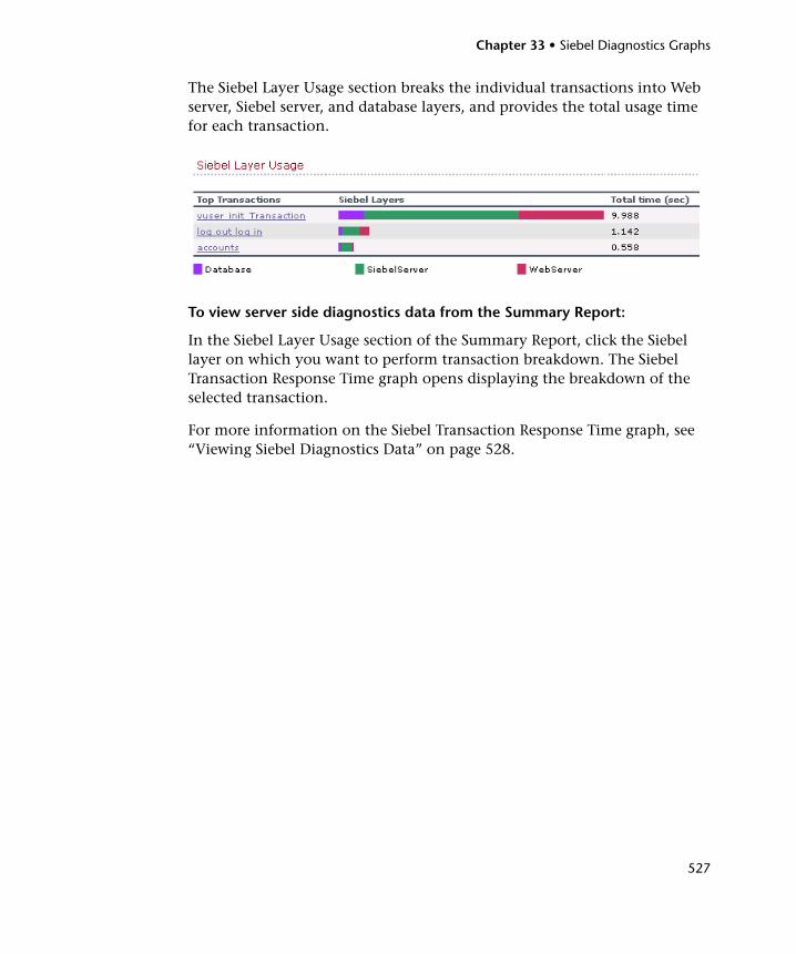
Chapter 33 • Siebel Diagnostics Graphs
527
The Siebel Layer Usage section breaks the individual transactions into Web server, Siebel server, and database layers, and provides the total usage time for each transaction.
To view server side diagnostics data from the Summary Report:
In the Siebel Layer Usage section of the Summary Report, click the Siebel layer on which you want to perform transaction breakdown. The Siebel Transaction Response Time graph opens displaying the breakdown of the selected transaction.
For more information on the Siebel Transaction Response Time graph, see “Viewing Siebel Diagnostics Data” on page 528.
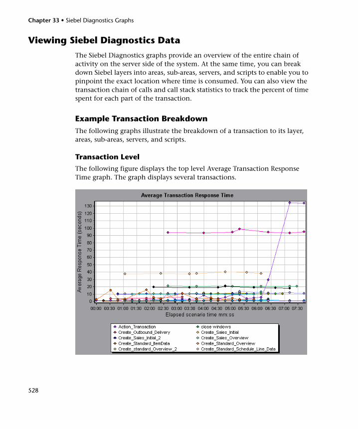
Chapter 33 • Siebel Diagnostics Graphs
528
Viewing Siebel Diagnostics Data
The Siebel Diagnostics graphs provide an overview of the entire chain of activity on the server side of the system. At the same time, you can break down Siebel layers into areas, sub-areas, servers, and scripts to enable you to pinpoint the exact location where time is consumed. You can also view the transaction chain of calls and call stack statistics to track the percent of time spent for each part of the transaction.
Example Transaction BreakdownThe following graphs illustrate the breakdown of a transaction to its layer, areas, sub-areas, servers, and scripts.
Transaction Level
The following figure displays the top level Average Transaction Response Time graph. The graph displays several transactions.
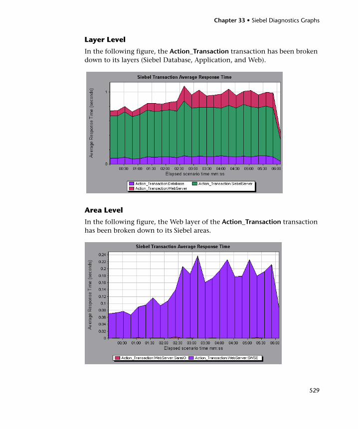
Chapter 33 • Siebel Diagnostics Graphs
529
Layer Level
In the following figure, the Action_Transaction transaction has been broken down to its layers (Siebel Database, Application, and Web).
Area Level
In the following figure, the Web layer of the Action_Transaction transaction has been broken down to its Siebel areas.
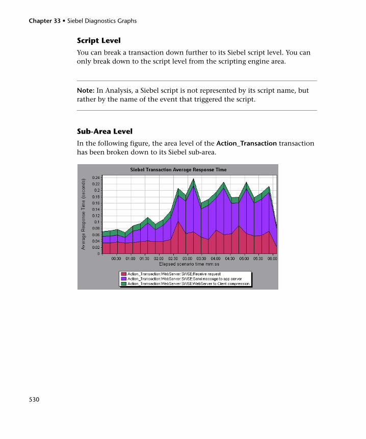
Chapter 33 • Siebel Diagnostics Graphs
530
Script Level
You can break a transaction down further to its Siebel script level. You can only break down to the script level from the scripting engine area.
Note: In Analysis, a Siebel script is not represented by its script name, but rather by the name of the event that triggered the script.
Sub-Area Level
In the following figure, the area level of the Action_Transaction transaction has been broken down to its Siebel sub-area.
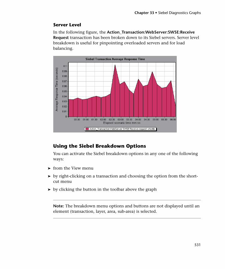
Chapter 33 • Siebel Diagnostics Graphs
531
Server Level
In the following figure, the Action_Transaction:WebServer:SWSE:Receive Request transaction has been broken down to its Siebel servers. Server level breakdown is useful for pinpointing overloaded servers and for load balancing.
Using the Siebel Breakdown OptionsYou can activate the Siebel breakdown options in any one of the following ways:
➤ from the View menu
➤ by right-clicking on a transaction and choosing the option from the short-cut menu
➤ by clicking the button in the toolbar above the graph
Note: The breakdown menu options and buttons are not displayed until an element (transaction, layer, area, sub-area) is selected.
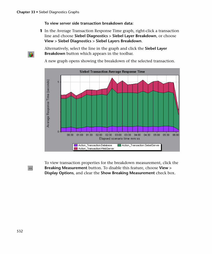
Chapter 33 • Siebel Diagnostics Graphs
532
To view server side transaction breakdown data:
1 In the Average Transaction Response Time graph, right-click a transaction line and choose Siebel Diagnostics > Siebel Layer Breakdown, or choose View > Siebel Diagnostics > Siebel Layers Breakdown.
Alternatively, select the line in the graph and click the Siebel Layer Breakdown button which appears in the toolbar.
A new graph opens showing the breakdown of the selected transaction.
To view transaction properties for the breakdown measurement, click the Breaking Measurement button. To disable this feature, choose View > Display Options, and clear the Show Breaking Measurement check box.
Chapter 33 • Siebel Diagnostics Graphs
533
2 You can select a displayed element and use the Siebel Breakdown menu or buttons to do the following:
➤ Break the data down to a lower level by selecting:
➤ Siebel Diagnostics > Siebel Area Breakdown, or click the Siebel Area Breakdown button to break the data down to its Siebel areas.
➤ Siebel Diagnostics > Siebel Sub-Area Breakdown, or click the Siebel Sub-Area Breakdown button to break the data down to its Siebel sub-areas. You can only break down to the sub-area level from the area level.
➤ Siebel Diagnostics > Siebel Script Breakdown, or click the Siebel Script Breakdown button to break the data down to its Siebel scripts. You can only break down to the script level from the scripting engine area.
Note: In Analysis, a Siebel script is not represented by its script name, but rather by the name of the event that triggered the script.
➤ Siebel Diagnostics > Siebel Server Breakdown, or click the Siebel Server Breakdown button to group the data by Siebel server.
➤ Return to a previous level by choosing:
➤ Siebel Diagnostics > Undo Siebel Sub-Area Breakdown, or click the Undo Siebel Sub-Area Breakdown button. This returns the graph to the area level.
➤ Siebel Diagnostics > Undo Siebel Area Breakdown, or click the Undo Siebel Area Breakdown button. This returns the graph to the layer level.
➤ Siebel Diagnostics > Undo Siebel Layer Breakdown, or click the Undo Siebel Layer Breakdown button. This returns the graph to the transaction level.
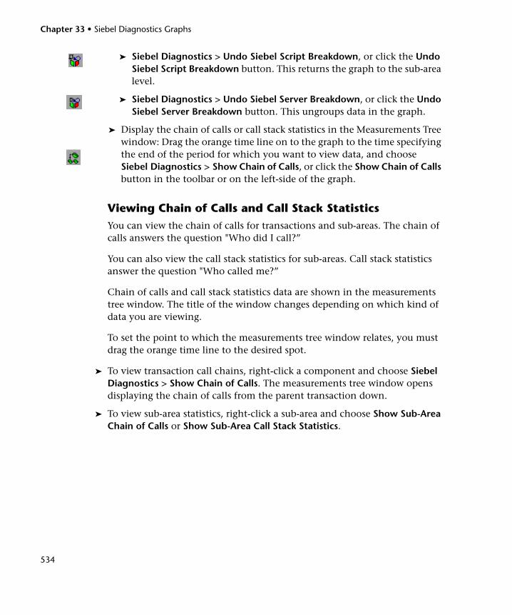
Chapter 33 • Siebel Diagnostics Graphs
534
➤ Siebel Diagnostics > Undo Siebel Script Breakdown, or click the Undo Siebel Script Breakdown button. This returns the graph to the sub-area level.
➤ Siebel Diagnostics > Undo Siebel Server Breakdown, or click the Undo Siebel Server Breakdown button. This ungroups data in the graph.
➤ Display the chain of calls or call stack statistics in the Measurements Tree window: Drag the orange time line on to the graph to the time specifying the end of the period for which you want to view data, and choose Siebel Diagnostics > Show Chain of Calls, or click the Show Chain of Calls button in the toolbar or on the left-side of the graph.
Viewing Chain of Calls and Call Stack StatisticsYou can view the chain of calls for transactions and sub-areas. The chain of calls answers the question "Who did I call?”
You can also view the call stack statistics for sub-areas. Call stack statistics answer the question "Who called me?”
Chain of calls and call stack statistics data are shown in the measurements tree window. The title of the window changes depending on which kind of data you are viewing.
To set the point to which the measurements tree window relates, you must drag the orange time line to the desired spot.
➤ To view transaction call chains, right-click a component and choose Siebel Diagnostics > Show Chain of Calls. The measurements tree window opens displaying the chain of calls from the parent transaction down.
➤ To view sub-area statistics, right-click a sub-area and choose Show Sub-Area Chain of Calls or Show Sub-Area Call Stack Statistics.
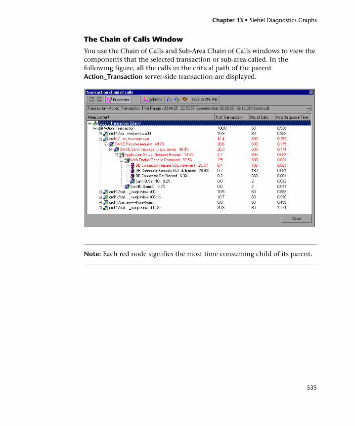
Chapter 33 • Siebel Diagnostics Graphs
535
The Chain of Calls Window
You use the Chain of Calls and Sub-Area Chain of Calls windows to view the components that the selected transaction or sub-area called. In the following figure, all the calls in the critical path of the parent Action_Transaction server-side transaction are displayed.
Note: Each red node signifies the most time consuming child of its parent.
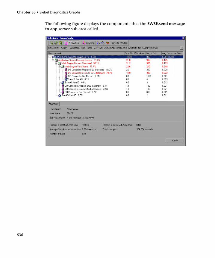
Chapter 33 • Siebel Diagnostics Graphs
536
The following figure displays the components that the SWSE.send message to app server sub-area called.
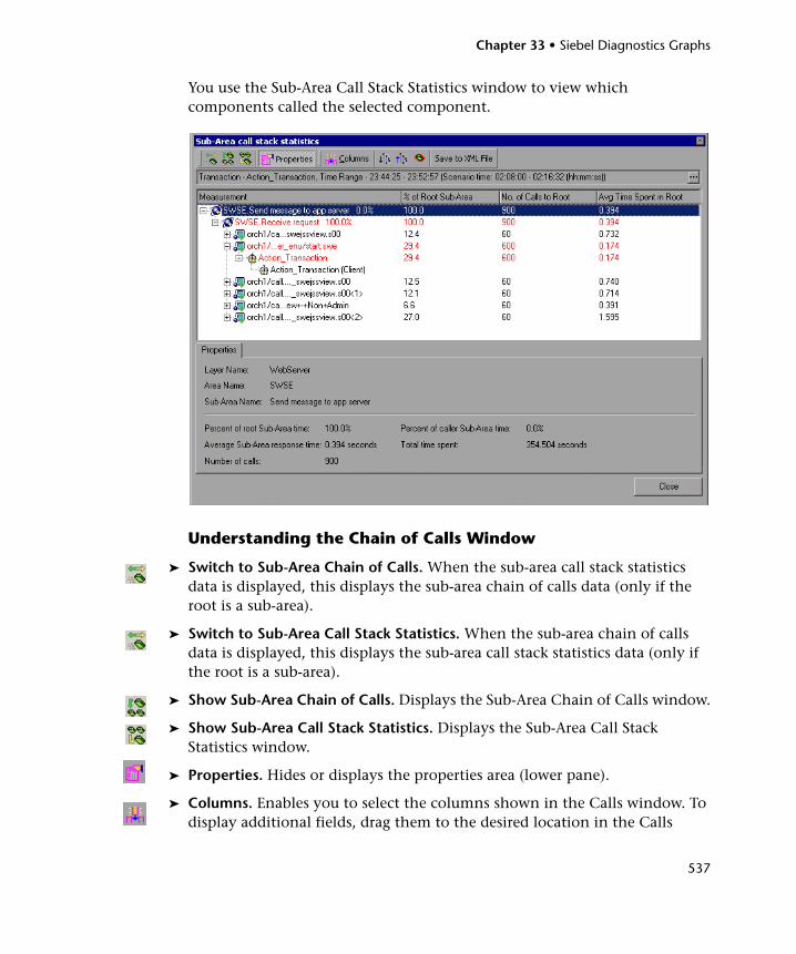
Chapter 33 • Siebel Diagnostics Graphs
537
You use the Sub-Area Call Stack Statistics window to view which components called the selected component.
Understanding the Chain of Calls Window
➤ Switch to Sub-Area Chain of Calls. When the sub-area call stack statistics data is displayed, this displays the sub-area chain of calls data (only if the root is a sub-area).
➤ Switch to Sub-Area Call Stack Statistics. When the sub-area chain of calls data is displayed, this displays the sub-area call stack statistics data (only if the root is a sub-area).
➤ Show Sub-Area Chain of Calls. Displays the Sub-Area Chain of Calls window.
➤ Show Sub-Area Call Stack Statistics. Displays the Sub-Area Call Stack Statistics window.
➤ Properties. Hides or displays the properties area (lower pane).
➤ Columns. Enables you to select the columns shown in the Calls window. To display additional fields, drag them to the desired location in the Calls

Chapter 33 • Siebel Diagnostics Graphs
538
window. To remove fields, drag them from the Calls window back to the Columns chooser.
The following columns are available in the Chain of Calls window:
Column Description
Measurement Name of the sub-area, displayed as AreaName:SubAreaName. In the case of a database call, query information is also displayed. The percent shown indicates the percentage of calls to this component from its parent.
% of Transaction/Root Sub-Area
Displays the percentage of sub-area time in relation the total transaction/root sub-area time.
No of Calls Displays the amount of times this transaction or sub-area was executed.
Avg Response Time Response time is the time from the beginning of execution until the end. Average response time is the total response time divided by the number of instances of the area/sub-area.
STD Response Time The standard deviation response time.
Min Response Time The minimum response time.
Max Response Time The maximum response time.
% of Caller Displays the percentage of sub-area time in relation the parent sub-area time.
Total time Displays the total sub-area execution time, including the child execution time.
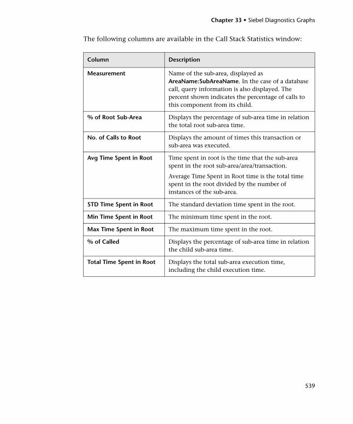
Chapter 33 • Siebel Diagnostics Graphs
539
The following columns are available in the Call Stack Statistics window:
Column Description
Measurement Name of the sub-area, displayed as AreaName:SubAreaName. In the case of a database call, query information is also displayed. The percent shown indicates the percentage of calls to this component from its child.
% of Root Sub-Area Displays the percentage of sub-area time in relation the total root sub-area time.
No. of Calls to Root Displays the amount of times this transaction or sub-area was executed.
Avg Time Spent in Root Time spent in root is the time that the sub-area spent in the root sub-area/area/transaction.
Average Time Spent in Root time is the total time spent in the root divided by the number of instances of the sub-area.
STD Time Spent in Root The standard deviation time spent in the root.
Min Time Spent in Root The minimum time spent in the root.
Max Time Spent in Root The maximum time spent in the root.
% of Called Displays the percentage of sub-area time in relation the child sub-area time.
Total Time Spent in Root Displays the total sub-area execution time, including the child execution time.
Chapter 33 • Siebel Diagnostics Graphs
540
➤ Expand All. Expands the entire tree.
➤ Collapse All. Collapses the entire tree.
➤ Expand Worst Path. Expands only the parts of the path on the critical path.
➤ Save to XML File. Saves the tree data to an XML file.
➤ Properties Area. Displays the full properties of the selected sub-area.
➤ SQL Query. Displays the SQL query for the selected sub-area. (For Database only.)
Available Siebel Diagnostics Graphs
This section includes:
➤ “Setting Graph Filter Properties” on page 541
➤ “Siebel Transaction Average Response Time Graph” on page 542
➤ “Siebel Area Average Response Time Graph” on page 543
➤ “Siebel Area Call Count Graph” on page 544
➤ “Siebel Area Total Response Time Graph” on page 545
➤ “Siebel Request Average Response Time Graph” on page 546
Note: To obtain diagnostics data for these graphs, you must enable the Siebel Diagnostics module (from the Controller) before running the scenario. For more information, refer to the LoadRunner Controller User’s Guide.
Chapter 33 • Siebel Diagnostics Graphs
541
Setting Graph Filter PropertiesYou can filter the Siebel Diagnostics graphs so that the displayed data is more suitable to your needs. You can filter using the following methods:
➤ Before opening a graph, enter filter criteria in the Graph Properties box of the Open a New Graph dialog box. For more information, see “Accessing and Opening Graphs and Reports” on page 30.
From an open graph, enter filter criteria in the Filter condition fields in a filter dialog box. For more information, see “Filtering and Sorting Graph Data” on page 79 and “Drilling Down in a Graph” on page 102.
➤ You can filter the Siebel graphs by the following fields:
Transaction Name. Shows data for the specified transaction.
Scenario Elapsed Time. Shows data for transactions that ended during the specified time.
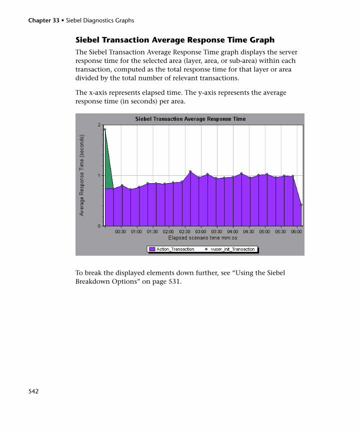
Chapter 33 • Siebel Diagnostics Graphs
542
Siebel Transaction Average Response Time GraphThe Siebel Transaction Average Response Time graph displays the server response time for the selected area (layer, area, or sub-area) within each transaction, computed as the total response time for that layer or area divided by the total number of relevant transactions.
The x-axis represents elapsed time. The y-axis represents the average response time (in seconds) per area.
To break the displayed elements down further, see “Using the Siebel Breakdown Options” on page 531.
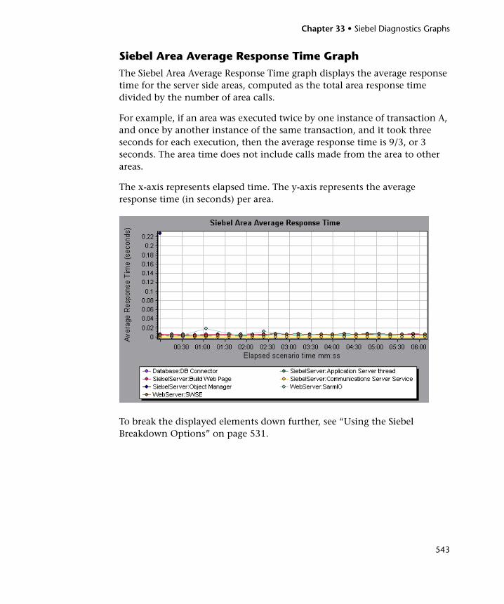
Chapter 33 • Siebel Diagnostics Graphs
543
Siebel Area Average Response Time GraphThe Siebel Area Average Response Time graph displays the average response time for the server side areas, computed as the total area response time divided by the number of area calls.
For example, if an area was executed twice by one instance of transaction A, and once by another instance of the same transaction, and it took three seconds for each execution, then the average response time is 9/3, or 3 seconds. The area time does not include calls made from the area to other areas.
The x-axis represents elapsed time. The y-axis represents the average response time (in seconds) per area.
To break the displayed elements down further, see “Using the Siebel Breakdown Options” on page 531.
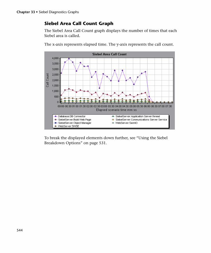
Chapter 33 • Siebel Diagnostics Graphs
544
Siebel Area Call Count GraphThe Siebel Area Call Count graph displays the number of times that each Siebel area is called.
The x-axis represents elapsed time. The y-axis represents the call count.
To break the displayed elements down further, see “Using the Siebel Breakdown Options” on page 531.
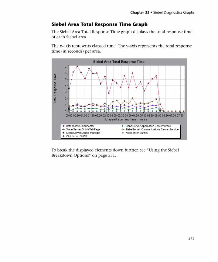
Chapter 33 • Siebel Diagnostics Graphs
545
Siebel Area Total Response Time GraphThe Siebel Area Total Response Time graph displays the total response time of each Siebel area.
The x-axis represents elapsed time. The y-axis represents the total response time (in seconds) per area.
To break the displayed elements down further, see “Using the Siebel Breakdown Options” on page 531.
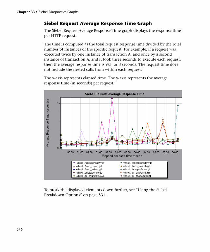
Chapter 33 • Siebel Diagnostics Graphs
546
Siebel Request Average Response Time GraphThe Siebel Request Average Response Time graph displays the response time per HTTP request.
The time is computed as the total request response time divided by the total number of instances of the specific request. For example, if a request was executed twice by one instance of transaction A, and once by a second instance of transaction A, and it took three seconds to execute each request, then the average response time is 9/3, or 3 seconds. The request time does not include the nested calls from within each request.
The x-axis represents elapsed time. The y-axis represents the average response time (in seconds) per request.
To break the displayed elements down further, see “Using the Siebel Breakdown Options” on page 531.
547
34 Siebel DB Diagnostics Graphs
After a load test scenario run, you use the Siebel DB Diagnostics graphs to analyze Siebel server performance.
This chapter includes:
➤ About Siebel DB Diagnostics Graphs on page 548
➤ Enabling Siebel DB Diagnostics on page 549
➤ Synchronizing Siebel Clock Settings on page 551
➤ Viewing Siebel DB Diagnostics Data on page 553
➤ Available Siebel DB Diagnostics Graphs on page 558
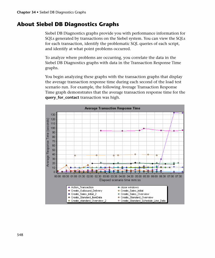
Chapter 34 • Siebel DB Diagnostics Graphs
548
About Siebel DB Diagnostics Graphs
Siebel DB Diagnostics graphs provide you with performance information for SQLs generated by transactions on the Siebel system. You can view the SQLs for each transaction, identify the problematic SQL queries of each script, and identify at what point problems occurred.
To analyze where problems are occurring, you correlate the data in the Siebel DB Diagnostics graphs with data in the Transaction Response Time graphs.
You begin analyzing these graphs with the transaction graphs that display the average transaction response time during each second of the load test scenario run. For example, the following Average Transaction Response Time graph demonstrates that the average transaction response time for the query_for_contact transaction was high.
Chapter 34 • Siebel DB Diagnostics Graphs
549
Using the Siebel DB Diagnostics graphs, you can pinpoint the cause of the delay in response time for this transaction.
Note: A measurement that is broken down in the Average Transaction Response Time graph will be different from the same measurement broken down in the Siebel DB Side Transactions graph. This is because the Average Transaction Response Time graph displays the average transaction time, whereas the Siebel DB Side Transactions graph displays the average time per transaction event (sum of SQL component response times).
Enabling Siebel DB Diagnostics
To generate Siebel DB diagnostics data, you must first install the ERP/CRM Mediator. For information on installing the Mediator, refer to the HP LoadRunner Installation Guide.
The Mediator is used to gather and correlate offline diagnostics data from the Siebel server. The Mediator processes the diagnostics data, and then passes it to the Controller.
Note: The Mediator must reside in the same LAN as the Siebel server.
To obtain diagnostics data for these graphs, you need to set up the Siebel DB Diagnostics module before running the scenario, and specify the sampling percentage of diagnostics data to include in the diagnostics graphs. For more information on configuring Siebel DB Diagnostics, refer to the HP LoadRunner Controller User Guide.
Chapter 34 • Siebel DB Diagnostics Graphs
550
Notes:
➤ You should not use the Data Time Range feature (Tools > Options > Result Collection > Data Time Range) when analyzing Siebel DB Diagnostics graphs since the data may be incomplete.
➤ The settings that you configure are per scenario. All scripts in the scenario will run under the same diagnostics configuration.
➤ To ensure that valid diagnostics data is generated, manually define the transactions in the Vuser script rather than using automatic transactions. Make sure to disable the following options in the Run-Time Settings’ General : Miscellaneous node: Define each action as a transaction and Define each step as a transaction.
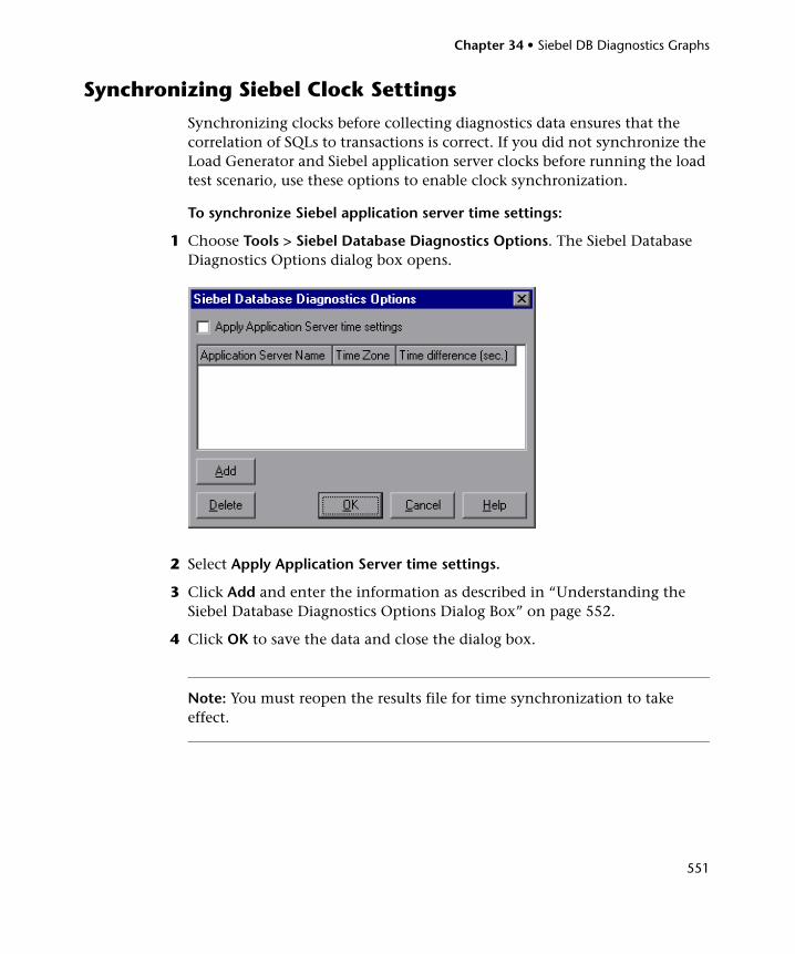
Chapter 34 • Siebel DB Diagnostics Graphs
551
Synchronizing Siebel Clock Settings
Synchronizing clocks before collecting diagnostics data ensures that the correlation of SQLs to transactions is correct. If you did not synchronize the Load Generator and Siebel application server clocks before running the load test scenario, use these options to enable clock synchronization.
To synchronize Siebel application server time settings:
1 Choose Tools > Siebel Database Diagnostics Options. The Siebel Database Diagnostics Options dialog box opens.
2 Select Apply Application Server time settings.
3 Click Add and enter the information as described in “Understanding the Siebel Database Diagnostics Options Dialog Box” on page 552.
4 Click OK to save the data and close the dialog box.
Note: You must reopen the results file for time synchronization to take effect.
Chapter 34 • Siebel DB Diagnostics Graphs
552
Understanding the Siebel Database Diagnostics Options Dialog BoxThe Siebel Database Diagnostics Options dialog box enables you to synchronize the Load Generator and Siebel application server clocks.
➤ Apply Application Server time settings. Enables the synchronized time settings option.
➤ Application Server Name. Enter the name of the Siebel application server.
➤ Time Zone. Enter the time zone of the Siebel application server (GMT or Local). GMT means the application server time is reported in GMT time, and local means the application server time is reported in local time.
➤ Time Difference (sec.). Enter the time difference (in seconds) between the load generator and the Siebel application server. Use the minus sign ("-") if the time on Siebel application server is ahead of the load generator . For example, if the application server time is two minutes ahead of the load generator time, enter -120 in the time difference field.
➤ Add. Enables you to add an application server’s time settings to the list.
➤ Delete. Deletes the server breakdown time settings from the list.
Note: You must reopen the results file for time synchronization to take effect.
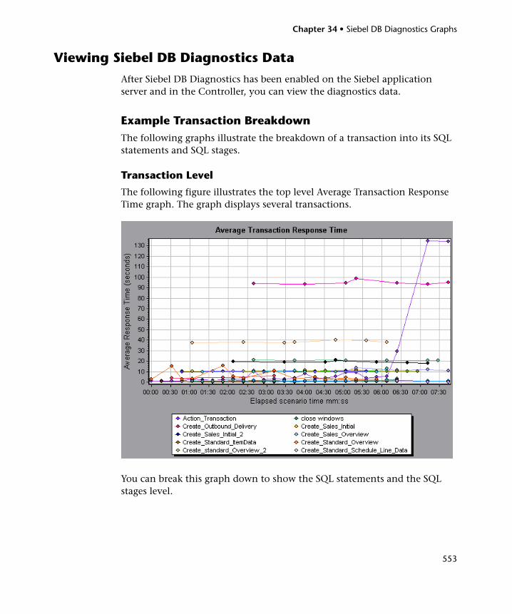
Chapter 34 • Siebel DB Diagnostics Graphs
553
Viewing Siebel DB Diagnostics Data
After Siebel DB Diagnostics has been enabled on the Siebel application server and in the Controller, you can view the diagnostics data.
Example Transaction BreakdownThe following graphs illustrate the breakdown of a transaction into its SQL statements and SQL stages.
Transaction Level
The following figure illustrates the top level Average Transaction Response Time graph. The graph displays several transactions.
You can break this graph down to show the SQL statements and the SQL stages level.
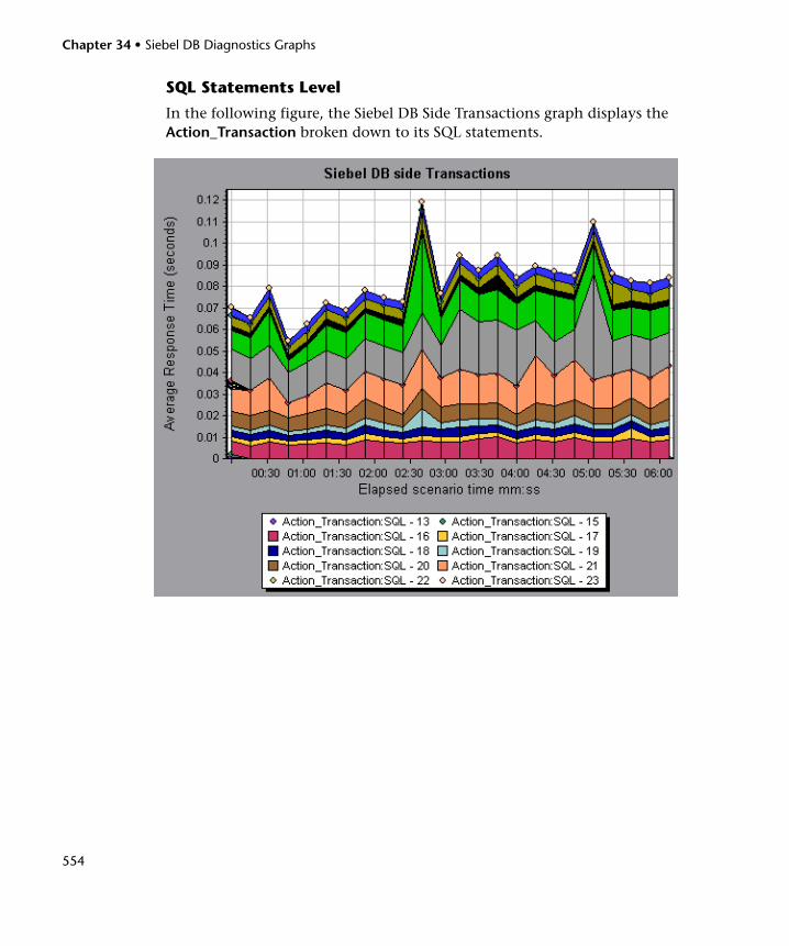
Chapter 34 • Siebel DB Diagnostics Graphs
554
SQL Statements Level
In the following figure, the Siebel DB Side Transactions graph displays the Action_Transaction broken down to its SQL statements.
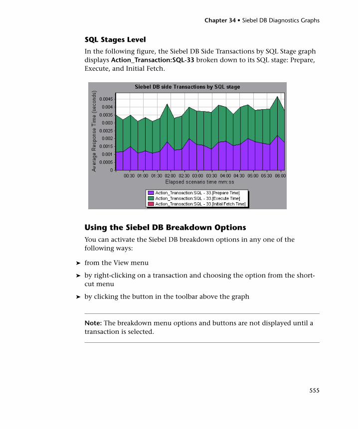
Chapter 34 • Siebel DB Diagnostics Graphs
555
SQL Stages Level
In the following figure, the Siebel DB Side Transactions by SQL Stage graph displays Action_Transaction:SQL-33 broken down to its SQL stage: Prepare, Execute, and Initial Fetch.
Using the Siebel DB Breakdown OptionsYou can activate the Siebel DB breakdown options in any one of the following ways:
➤ from the View menu
➤ by right-clicking on a transaction and choosing the option from the short-cut menu
➤ by clicking the button in the toolbar above the graph
Note: The breakdown menu options and buttons are not displayed until a transaction is selected.
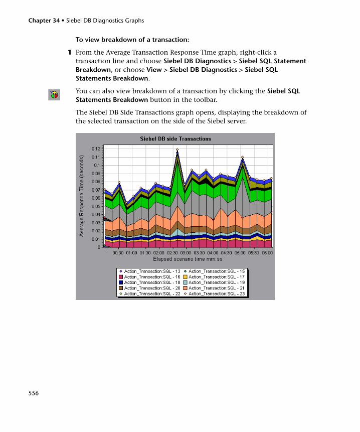
Chapter 34 • Siebel DB Diagnostics Graphs
556
To view breakdown of a transaction:
1 From the Average Transaction Response Time graph, right-click a transaction line and choose Siebel DB Diagnostics > Siebel SQL Statement Breakdown, or choose View > Siebel DB Diagnostics > Siebel SQL Statements Breakdown.
You can also view breakdown of a transaction by clicking the Siebel SQL Statements Breakdown button in the toolbar.
The Siebel DB Side Transactions graph opens, displaying the breakdown of the selected transaction on the side of the Siebel server.
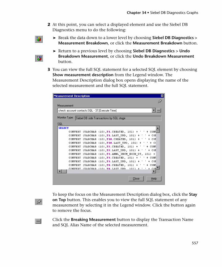
Chapter 34 • Siebel DB Diagnostics Graphs
557
2 At this point, you can select a displayed element and use the Siebel DB Diagnostics menu to do the following:
➤ Break the data down to a lower level by choosing Siebel DB Diagnostics > Measurement Breakdown, or click the Measurement Breakdown button.
➤ Return to a previous level by choosing Siebel DB Diagnostics > Undo Breakdown Measurement, or click the Undo Breakdown Measurement button.
3 You can view the full SQL statement for a selected SQL element by choosing Show measurement description from the Legend window. The Measurement Description dialog box opens displaying the name of the selected measurement and the full SQL statement.
To keep the focus on the Measurement Description dialog box, click the Stay on Top button. This enables you to view the full SQL statement of any measurement by selecting it in the Legend window. Click the button again to remove the focus.
Click the Breaking Measurement button to display the Transaction Name and SQL Alias Name of the selected measurement.
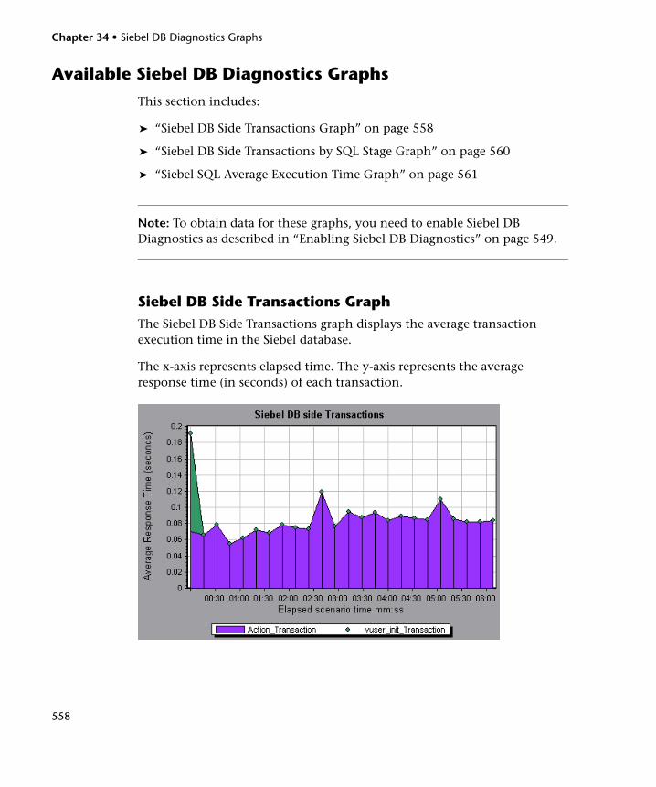
Chapter 34 • Siebel DB Diagnostics Graphs
558
Available Siebel DB Diagnostics Graphs
This section includes:
➤ “Siebel DB Side Transactions Graph” on page 558
➤ “Siebel DB Side Transactions by SQL Stage Graph” on page 560
➤ “Siebel SQL Average Execution Time Graph” on page 561
Note: To obtain data for these graphs, you need to enable Siebel DB Diagnostics as described in “Enabling Siebel DB Diagnostics” on page 549.
Siebel DB Side Transactions GraphThe Siebel DB Side Transactions graph displays the average transaction execution time in the Siebel database.
The x-axis represents elapsed time. The y-axis represents the average response time (in seconds) of each transaction.
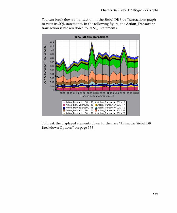
Chapter 34 • Siebel DB Diagnostics Graphs
559
You can break down a transaction in the Siebel DB Side Transactions graph to view its SQL statements. In the following figure, the Action_Transaction transaction is broken down to its SQL statements.
To break the displayed elements down further, see “Using the Siebel DB Breakdown Options” on page 555.
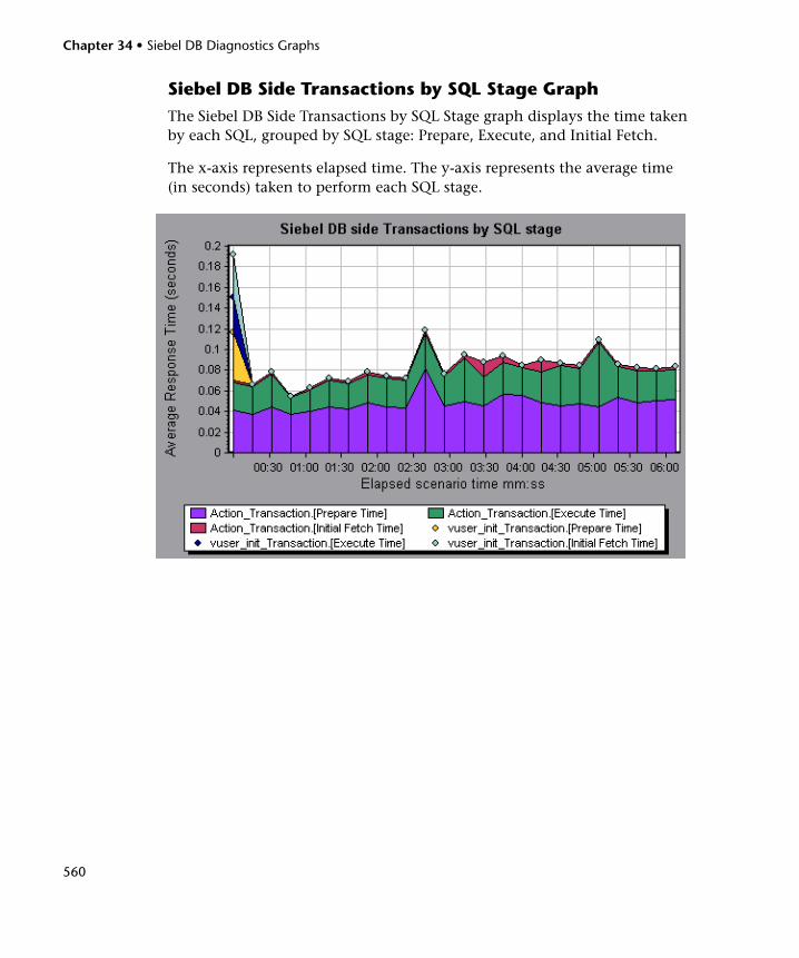
Chapter 34 • Siebel DB Diagnostics Graphs
560
Siebel DB Side Transactions by SQL Stage GraphThe Siebel DB Side Transactions by SQL Stage graph displays the time taken by each SQL, grouped by SQL stage: Prepare, Execute, and Initial Fetch.
The x-axis represents elapsed time. The y-axis represents the average time (in seconds) taken to perform each SQL stage.
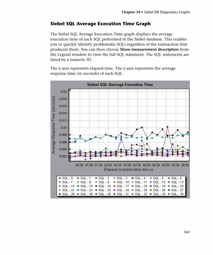
Chapter 34 • Siebel DB Diagnostics Graphs
561
Siebel SQL Average Execution Time Graph
The Siebel SQL Average Execution Time graph displays the average execution time of each SQL performed in the Siebel database. This enables you to quickly identify problematic SQLs regardless of the transaction that produced them. You can then choose Show measurement description from the Legend window to view the full SQL statement. The SQL statements are listed by a numeric ID.
The x-axis represents elapsed time. The y-axis represents the average response time (in seconds) of each SQL.

Chapter 34 • Siebel DB Diagnostics Graphs
562
563
35 Oracle 11i Diagnostics Graphs
After a load test scenario run, you can use the Oracle 11i Diagnostics graphs to analyze Oracle NCA server performance.
This chapter includes:
➤ About Oracle 11i Diagnostics Graphs on page 564
➤ Enabling Oracle 11i Diagnostics on page 565
➤ Viewing Oracle 11i Diagnostics Data on page 567
➤ Available Oracle 11i Diagnostics Graphs on page 572
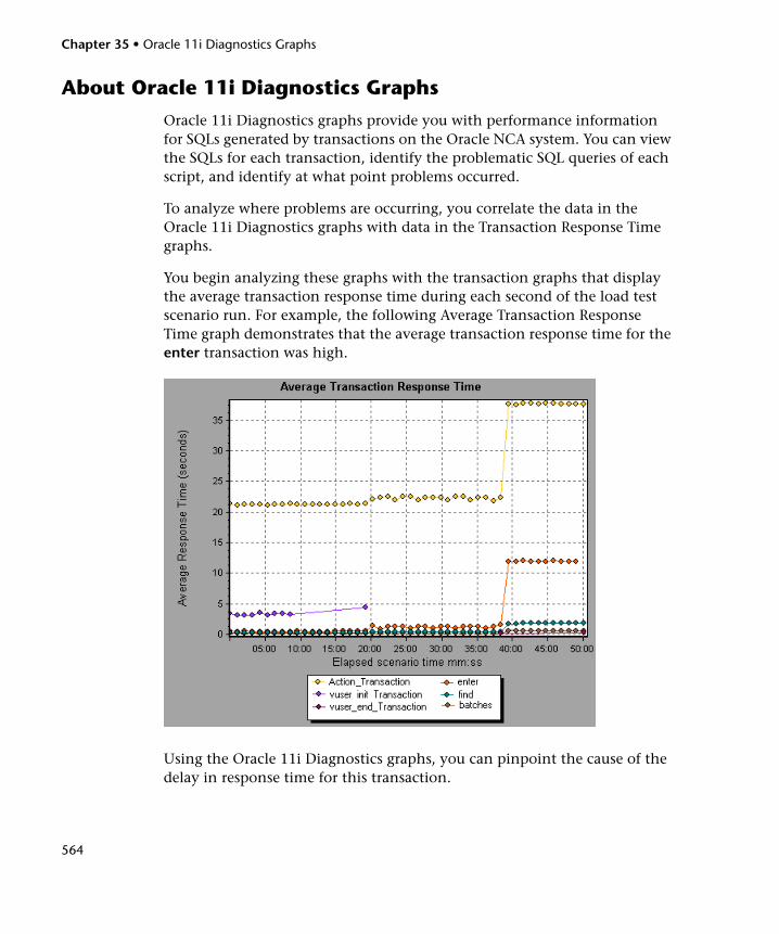
Chapter 35 • Oracle 11i Diagnostics Graphs
564
About Oracle 11i Diagnostics Graphs
Oracle 11i Diagnostics graphs provide you with performance information for SQLs generated by transactions on the Oracle NCA system. You can view the SQLs for each transaction, identify the problematic SQL queries of each script, and identify at what point problems occurred.
To analyze where problems are occurring, you correlate the data in the Oracle 11i Diagnostics graphs with data in the Transaction Response Time graphs.
You begin analyzing these graphs with the transaction graphs that display the average transaction response time during each second of the load test scenario run. For example, the following Average Transaction Response Time graph demonstrates that the average transaction response time for the enter transaction was high.
Using the Oracle 11i Diagnostics graphs, you can pinpoint the cause of the delay in response time for this transaction.
Chapter 35 • Oracle 11i Diagnostics Graphs
565
Notes:
➤ A measurement that is broken down in the Average Transaction Response Time graph will be different from the same measurement broken down in the Oracle 11i Side Transactions graph. This is because the Average Transaction Response Time graph displays the average transaction time, whereas the Oracle 11i Side Transactions graph displays the average time per transaction event (sum of SQL component response times).
➤ vuser_init and vuser_end actions in Oracle cannot be broken down. For more information, refer to the HP Virtual User Generator User Guide.
Enabling Oracle 11i Diagnostics
To generate Oracle 11i Diagnostics data, you must first install the ERP/CRM Mediator. For information on installing the Mediator, refer to the HP LoadRunner Installation Guide.
The Mediator is used to gather and correlate offline diagnostics data from the Oracle server. The Mediator processes the diagnostics data, and then passes it to the Controller.
Note: The Mediator must reside in the same LAN as the Oracle server.
Chapter 35 • Oracle 11i Diagnostics Graphs
566
To obtain diagnostics data for these graphs, you need to set up the Oracle 11i Diagnostics module before running the scenario, and specify the sampling percentage of diagnostics data to include in the diagnostics graphs. For more information on configuring Oracle 11i Diagnostics, refer to the HP LoadRunner Controller User Guide.
Notes:
➤ The settings that you configure are per scenario. All scripts in the scenario will run under the same diagnostics configuration.
➤ To ensure that valid diagnostics data is generated, manually define the transactions in the Vuser script rather than using automatic transactions. Make sure to disable the following options in the Run-Time Settings’ General : Miscellaneous node: Define each action as a transaction and Define each step as a transaction.
➤ If the Oracle 11i trace cannot be enabled automatically using the built-in mechanism, you can enable it manually in the Vuser script using the nca_set_custom_dbtrace and nca_set_dbtrace_file_index functions. This may occur if you are using a custom application that does not have a standard UI.
➤ You should not use the Data Time Range feature (Tools > Options > Result Collection > Data Time Range) when analyzing Oracle 11i Diagnostics graphs since the data may be incomplete.
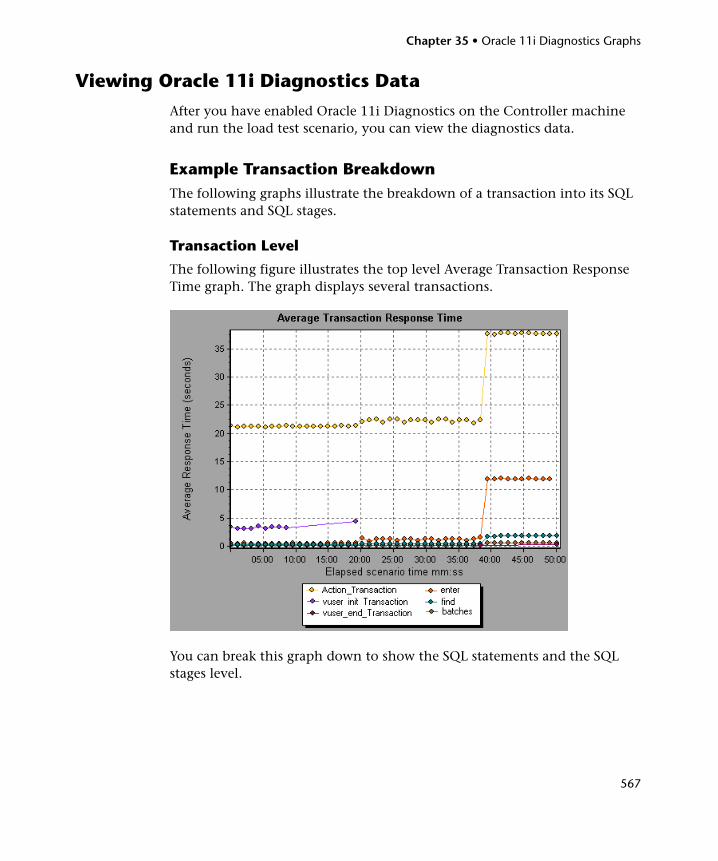
Chapter 35 • Oracle 11i Diagnostics Graphs
567
Viewing Oracle 11i Diagnostics Data
After you have enabled Oracle 11i Diagnostics on the Controller machine and run the load test scenario, you can view the diagnostics data.
Example Transaction BreakdownThe following graphs illustrate the breakdown of a transaction into its SQL statements and SQL stages.
Transaction Level
The following figure illustrates the top level Average Transaction Response Time graph. The graph displays several transactions.
You can break this graph down to show the SQL statements and the SQL stages level.
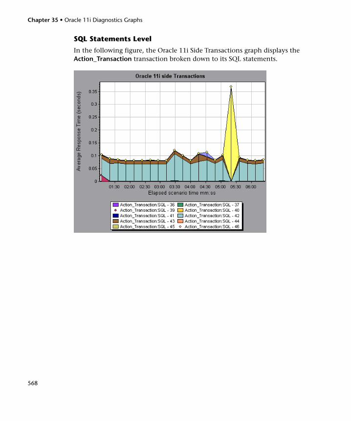
Chapter 35 • Oracle 11i Diagnostics Graphs
568
SQL Statements Level
In the following figure, the Oracle 11i Side Transactions graph displays the Action_Transaction transaction broken down to its SQL statements.
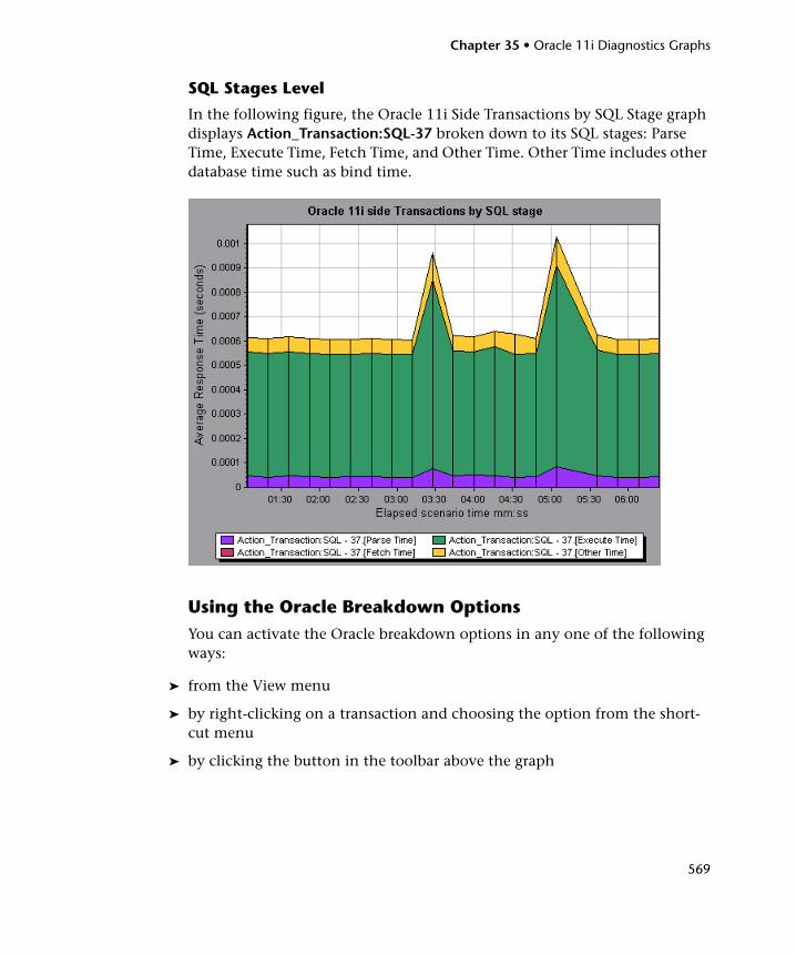
Chapter 35 • Oracle 11i Diagnostics Graphs
569
SQL Stages Level
In the following figure, the Oracle 11i Side Transactions by SQL Stage graph displays Action_Transaction:SQL-37 broken down to its SQL stages: Parse Time, Execute Time, Fetch Time, and Other Time. Other Time includes other database time such as bind time.
Using the Oracle Breakdown OptionsYou can activate the Oracle breakdown options in any one of the following ways:
➤ from the View menu
➤ by right-clicking on a transaction and choosing the option from the short-cut menu
➤ by clicking the button in the toolbar above the graph
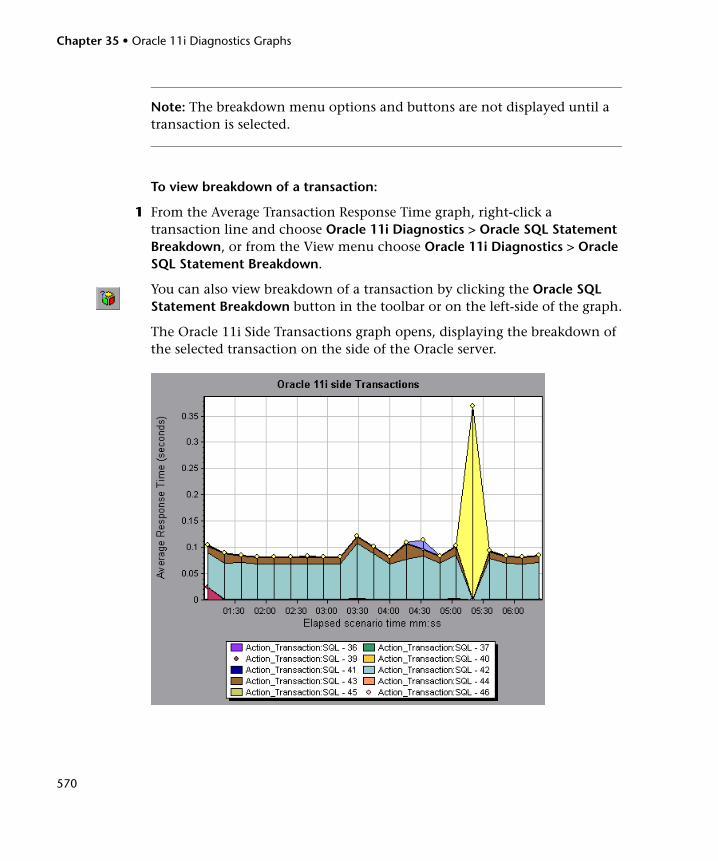
Chapter 35 • Oracle 11i Diagnostics Graphs
570
Note: The breakdown menu options and buttons are not displayed until a transaction is selected.
To view breakdown of a transaction:
1 From the Average Transaction Response Time graph, right-click a transaction line and choose Oracle 11i Diagnostics > Oracle SQL Statement Breakdown, or from the View menu choose Oracle 11i Diagnostics > Oracle SQL Statement Breakdown.
You can also view breakdown of a transaction by clicking the Oracle SQL Statement Breakdown button in the toolbar or on the left-side of the graph.
The Oracle 11i Side Transactions graph opens, displaying the breakdown of the selected transaction on the side of the Oracle server.
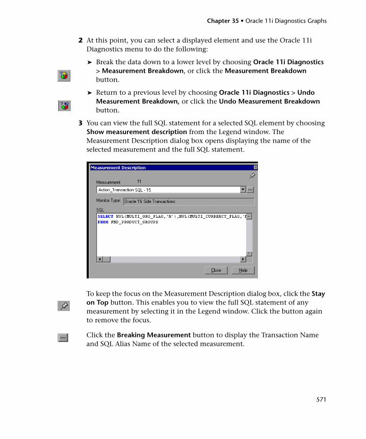
Chapter 35 • Oracle 11i Diagnostics Graphs
571
2 At this point, you can select a displayed element and use the Oracle 11i Diagnostics menu to do the following:
➤ Break the data down to a lower level by choosing Oracle 11i Diagnostics > Measurement Breakdown, or click the Measurement Breakdown button.
➤ Return to a previous level by choosing Oracle 11i Diagnostics > Undo Measurement Breakdown, or click the Undo Measurement Breakdown button.
3 You can view the full SQL statement for a selected SQL element by choosing Show measurement description from the Legend window. The Measurement Description dialog box opens displaying the name of the selected measurement and the full SQL statement.
To keep the focus on the Measurement Description dialog box, click the Stay on Top button. This enables you to view the full SQL statement of any measurement by selecting it in the Legend window. Click the button again to remove the focus.
Click the Breaking Measurement button to display the Transaction Name and SQL Alias Name of the selected measurement.
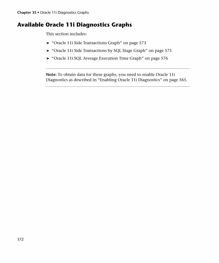
Chapter 35 • Oracle 11i Diagnostics Graphs
572
Available Oracle 11i Diagnostics Graphs
This section includes:
➤ “Oracle 11i Side Transactions Graph” on page 573
➤ “Oracle 11i Side Transactions by SQL Stage Graph” on page 575
➤ “Oracle 11i SQL Average Execution Time Graph” on page 576
Note: To obtain data for these graphs, you need to enable Oracle 11i Diagnostics as described in “Enabling Oracle 11i Diagnostics” on page 565.
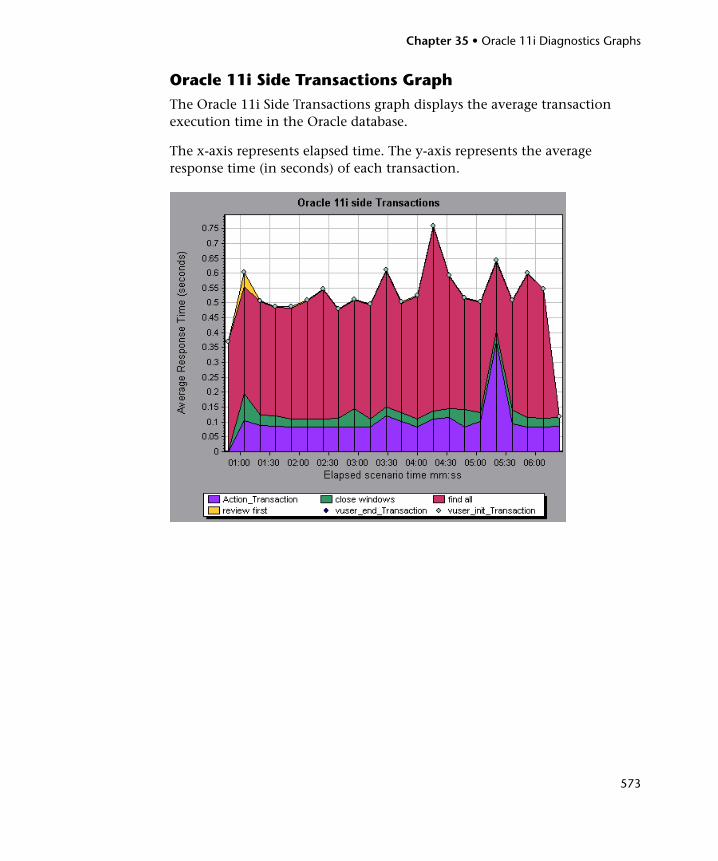
Chapter 35 • Oracle 11i Diagnostics Graphs
573
Oracle 11i Side Transactions GraphThe Oracle 11i Side Transactions graph displays the average transaction execution time in the Oracle database.
The x-axis represents elapsed time. The y-axis represents the average response time (in seconds) of each transaction.
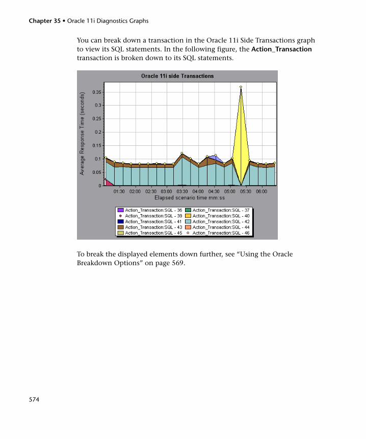
Chapter 35 • Oracle 11i Diagnostics Graphs
574
You can break down a transaction in the Oracle 11i Side Transactions graph to view its SQL statements. In the following figure, the Action_Transaction transaction is broken down to its SQL statements.
To break the displayed elements down further, see “Using the Oracle Breakdown Options” on page 569.
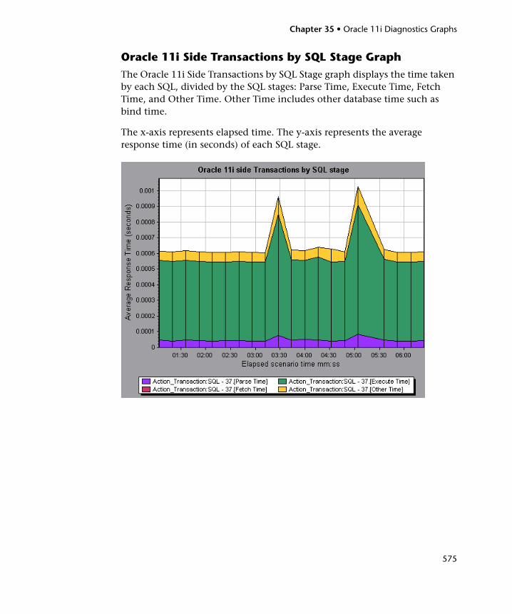
Chapter 35 • Oracle 11i Diagnostics Graphs
575
Oracle 11i Side Transactions by SQL Stage GraphThe Oracle 11i Side Transactions by SQL Stage graph displays the time taken by each SQL, divided by the SQL stages: Parse Time, Execute Time, Fetch Time, and Other Time. Other Time includes other database time such as bind time.
The x-axis represents elapsed time. The y-axis represents the average response time (in seconds) of each SQL stage.
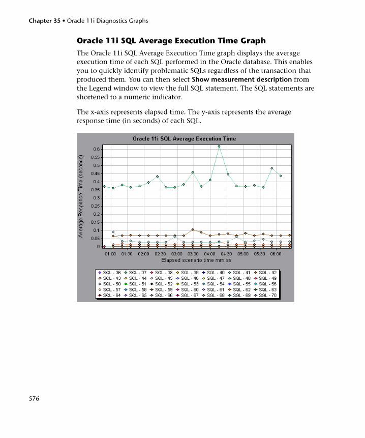
Chapter 35 • Oracle 11i Diagnostics Graphs
576
Oracle 11i SQL Average Execution Time GraphThe Oracle 11i SQL Average Execution Time graph displays the average execution time of each SQL performed in the Oracle database. This enables you to quickly identify problematic SQLs regardless of the transaction that produced them. You can then select Show measurement description from the Legend window to view the full SQL statement. The SQL statements are shortened to a numeric indicator.
The x-axis represents elapsed time. The y-axis represents the average response time (in seconds) of each SQL.
577
36 SAP Diagnostics Graphs
After a load test scenario run, you use the SAP Diagnostics graphs to analyze SAP server performance.
This chapter includes:
➤ About SAP Diagnostics Graphs on page 578
➤ Enabling SAP Diagnostics on page 578
➤ Viewing SAP Diagnostics Data on page 579
➤ Viewing the SAP Diagnostics in the Summary Report on page 583
➤ SAP Alerts on page 585
➤ Using the SAP Breakdown Options on page 589
➤ Available SAP Diagnostics Graphs on page 592
➤ SAP Secondary Graphs on page 600
Chapter 36 • SAP Diagnostics Graphs
578
About SAP Diagnostics Graphs
SAP Diagnostics enables you to pinpoint the root cause of a certain problem (i.e. DBA, Network, WAS, Application, OS/HW) quickly and easily, and engage with the relevant expert only, without having to present the problem to a whole team of people.
Using SAP Diagnostics, you can create graphs and reports, which you can present to the relevant expert when discussing the problems that occurred.
SAP Diagnostics also allow an SAP performance expert (in one of the areas of expertise) to perform the required root-cause analysis more quickly and easily.
Enabling SAP Diagnostics
To generate SAP diagnostics data, you must first install the ERP/CRM Mediator. For information on installing the Mediator, refer to the HP LoadRunner Installation Guide.
The Mediator component is used to gather and correlate offline diagnostics data from the SAP server. The Mediator processes the diagnostics data, and then passes it to the Controller.
To obtain diagnostics data for these graphs, you need to set up the SAP Diagnostics module before running the load test scenario, and specify the sampling percentage of diagnostics data to include in the diagnotsics graphs. For more information on configuring SAP Diagnostics, refer to the HP LoadRunner Controller User’s Guide.
Important Notes
➤ In order for SAP Diagnostics to perform effectively, it relies on sound and consistent performance of the SAP software. Malformation or inappropriate configuration of the SAP software could cause inaccuracies in SAP Diagnostics data collection.
Chapter 36 • SAP Diagnostics Graphs
579
➤ To ensure that valid diagnostics data is generated, manually define the transactions in the Vuser script rather than using automatic transactions. Make sure to disable the following options in the Run-Time Settings’ General : Miscellaneous node: Define each action as a transaction and Define each step as a transaction.
➤ The ERP/CRM Mediator requires an installation of SAPGUI 6.20 or 6.40.
➤ If no connection can be established between the ERP/CRM Mediator and one of the SAP application servers, no work process or OS monitor data is collected for that server. However, as long as there is a connection to one of the servers, statistical records for response time breakdown are still available.
➤ The settings that you configure are per scenario. All scripts in the scenario will run under the same diagnostics configuration.
Viewing SAP Diagnostics Data
The SAP Diagnostics graphs provide an overview of the entire chain of SAP activity on the server side of the system.
When the user drills down and explores SAP data and tries to locate possible problems, a guided flow sequence of interactive views is presented, and can be correlated over time with secondary graphs.
Opening SAP Diagnostics GraphsYou open the SAP Diagnostics graphs from the Analysis Summary Report or from the Open a New Graph dialog box.
To open SAP Diagnostics graphs from the Analysis Summary Report:
Click the View SAP Diagnostics link.
To open SAP Diagnostics graphs from the Session Explorer:
1 Click the Add New Graph button in the Session Explorer window. The Open a New Graph dialog box opens.
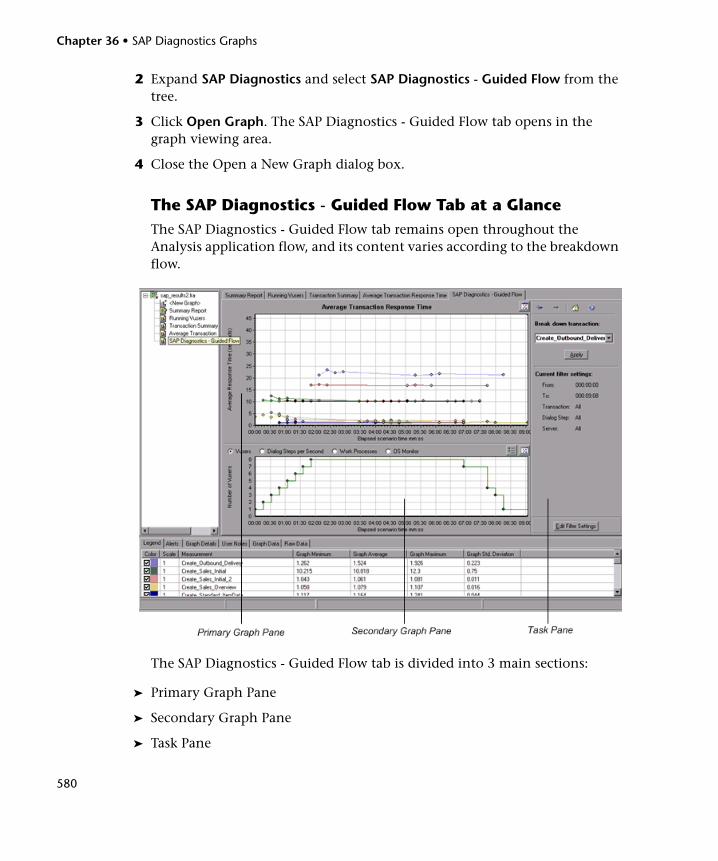
Chapter 36 • SAP Diagnostics Graphs
580
2 Expand SAP Diagnostics and select SAP Diagnostics - Guided Flow from the tree.
3 Click Open Graph. The SAP Diagnostics - Guided Flow tab opens in the graph viewing area.
4 Close the Open a New Graph dialog box.
The SAP Diagnostics - Guided Flow Tab at a GlanceThe SAP Diagnostics - Guided Flow tab remains open throughout the Analysis application flow, and its content varies according to the breakdown flow.
The SAP Diagnostics - Guided Flow tab is divided into 3 main sections:
➤ Primary Graph Pane
➤ Secondary Graph Pane
➤ Task Pane
Chapter 36 • SAP Diagnostics Graphs
581
Primary Graph Pane
The upper pane of the SAP Diagnostics - Guided Flow tab is referred to as the primary graph pane. This pane displays graphs of the transactions and their broken down dialog steps or components, and other associated resources.
You break down the graphs displayed in this pane using the breakdown options provided in the right pane of the guided flow (see Task Pane). For more information on applying breakdown options to transactions, see “Using the SAP Breakdown Options” on page 589.
You can open the displayed graph in full view by clicking the Enlarge Graph button in the top right corner of this pane. An enlarged version of the graph opens in a new tab.
Secondary Graph Pane
The lower pane of the SAP Diagnostics - Guided Flow tab is referred to as the secondary graph pane and displays graphs showing secondary information supporting the graph displayed in the primary graph pane.
To see the legend for the graph displayed in this pane, click the Graph Legend button in the top right corner. To see all the data in the Legend, scroll along the horizontal scroll bar.
You can open the displayed graph in full view by clicking the Enlarge Graph button in the top right corner of this pane. An enlarged version of the graph opens in a new tab.
Task Pane
The pane on the right side of the SAP Diagnostics - Guided Flow tab is referred to as the task pane. You use the task pane to choose the level of breakdown you want to view, to filter and group transaction and server information, and to navigate backwards and forwards through the broken down graphs.
For more information see “Using the SAP Breakdown Options” on page 589.
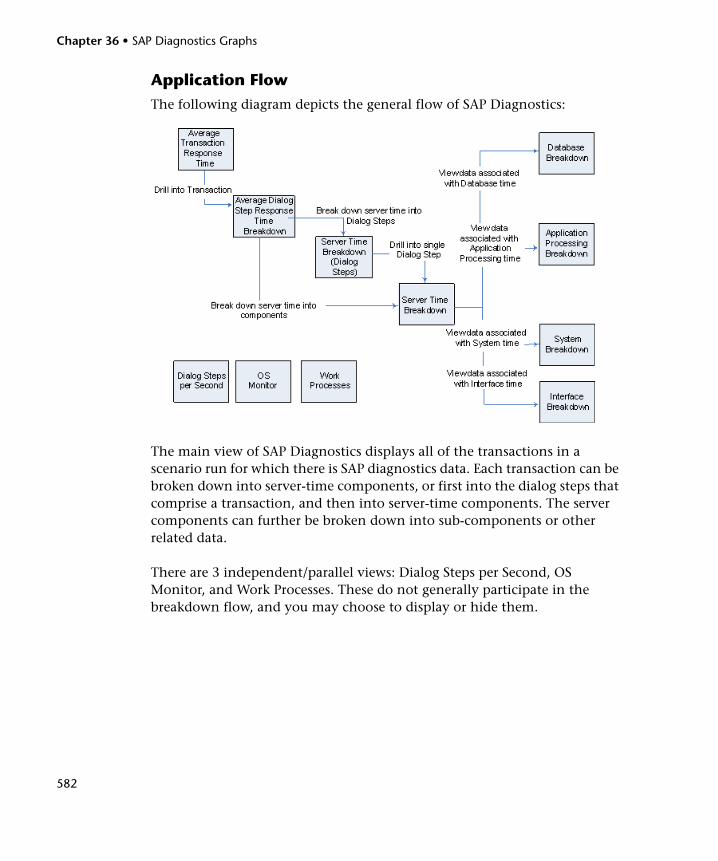
Chapter 36 • SAP Diagnostics Graphs
582
Application FlowThe following diagram depicts the general flow of SAP Diagnostics:
The main view of SAP Diagnostics displays all of the transactions in a scenario run for which there is SAP diagnostics data. Each transaction can be broken down into server-time components, or first into the dialog steps that comprise a transaction, and then into server-time components. The server components can further be broken down into sub-components or other related data.
There are 3 independent/parallel views: Dialog Steps per Second, OS Monitor, and Work Processes. These do not generally participate in the breakdown flow, and you may choose to display or hide them.
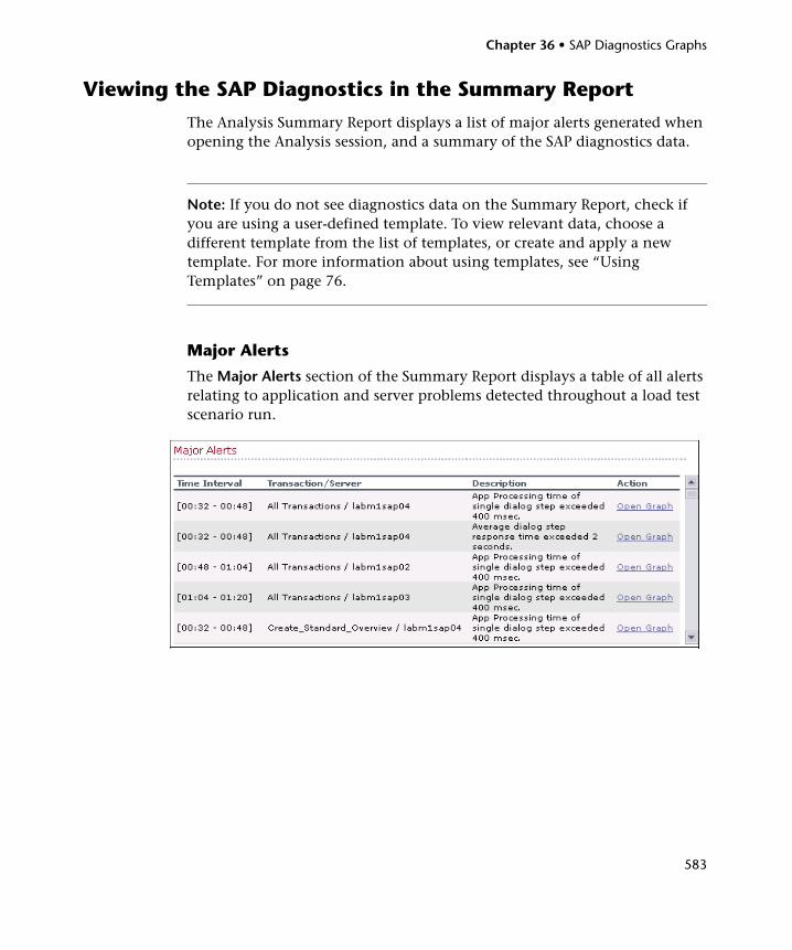
Chapter 36 • SAP Diagnostics Graphs
583
Viewing the SAP Diagnostics in the Summary Report
The Analysis Summary Report displays a list of major alerts generated when opening the Analysis session, and a summary of the SAP diagnostics data.
Note: If you do not see diagnostics data on the Summary Report, check if you are using a user-defined template. To view relevant data, choose a different template from the list of templates, or create and apply a new template. For more information about using templates, see “Using Templates” on page 76.
Major Alerts
The Major Alerts section of the Summary Report displays a table of all alerts relating to application and server problems detected throughout a load test scenario run.
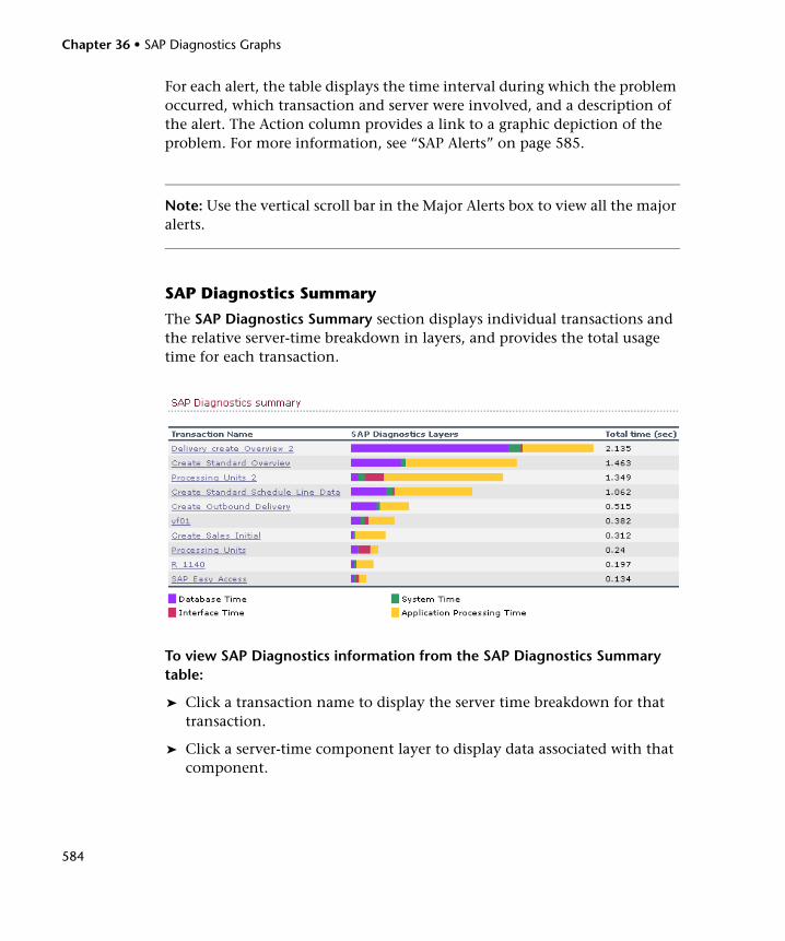
Chapter 36 • SAP Diagnostics Graphs
584
For each alert, the table displays the time interval during which the problem occurred, which transaction and server were involved, and a description of the alert. The Action column provides a link to a graphic depiction of the problem. For more information, see “SAP Alerts” on page 585.
Note: Use the vertical scroll bar in the Major Alerts box to view all the major alerts.
SAP Diagnostics Summary
The SAP Diagnostics Summary section displays individual transactions and the relative server-time breakdown in layers, and provides the total usage time for each transaction.
To view SAP Diagnostics information from the SAP Diagnostics Summary table:
➤ Click a transaction name to display the server time breakdown for that transaction.
➤ Click a server-time component layer to display data associated with that component.
Chapter 36 • SAP Diagnostics Graphs
585
SAP Alerts
SAP alerts pinpoint problems that arise during a load test scenario run, making it easier for the user to locate them. There are 2 types of alerts: standard and major, each of which is discussed in detail later in this section.
SAP Diagnostics comes with a set of alert conditions with pre-defined threshold values. If a threshold value is exceeded, SAP alerts the user that there is a problem. For example, if the average dialog step response time is greater than the pre-defined threshold value, an alert is generated.
This section includes:
➤ Viewing SAP Alerts
➤ Configuring SAP Alerts
Viewing SAP AlertsYou can view alerts in the Summary Report or in the SAP Alerts window (Windows > SAP Alerts).
The Major Alerts section of the Summary Report displays a list of all the major alerts generated during the load test scenario run, including information about when the problem occurred, which transaction or server was involved, and what the problem.
The SAP Alerts window (Windows > SAP Alerts) displays a list of alerts related to the data displayed in the current graph(s) shown in the Analysis window.
Notes:
➤ In the SAP Diagnostics - Guided Flow tab, alerts listed in the legend relate to the graphs displayed in both the primary graph and secondary graph panes.
➤ Applying filters or grouping to the primary graph affects which alerts are listed in the legend area.
Chapter 36 • SAP Diagnostics Graphs
586
The SAP Alerts window displays the following information:
➤ Type. Displays an icon indicating the type of alert.
➤ Standard Alert. This alert is generated in the context of a transaction and/or server if the conditions of a pre-defined alert rule are met.
➤ Major Alert. There are 2 types of major alerts:
➤ General Application Problem Alert. If a standard alert was generated in the context of a transaction, and the same alert was generated in the context of all other transactions running in the same time frame, then a major alert of this type is generated, indicating that there is a general application problem.
Note: If a Dialog Step filter is applied (for a single dialog step), then this alert is not generated.
➤ Server-Specific Problem Alert. This alert is generated for a specific server if a certain measurement on that server exceeds its threshold, while the overall server performance for that measurement is satisfactory. This type of alert indicates that there is a server related problem.
Note: Server-Specific Problem alerts are generated only when the current server context is "All Servers”.
For information about configuring alert rules, see “Configuring SAP Alerts” on page 587.
➤ Time interval. The time interval during which the problem occurred.
➤ Transaction/Server. The name of the transaction and server where problem occurred.
➤ Description. A description of the alert.
Chapter 36 • SAP Diagnostics Graphs
587
➤ Recommended Step. Recommends what to do in order to understand the problem on a deeper level.
➤ Action. A link to a graph representing the data described in the alert, allowing for a more graphic display of the alert. Double-click the link to open the graph.
Configuring SAP AlertsSAP Diagnostics comes with a set of alert rules with pre-defined threshold values.
When you open a LoadRunner results file (.lrr) in Analysis, these alert rules are applied to the load test scenario results, and if a threshold value is exceeded, Analysis generates an alert that there is a problem.
Before opening a LoadRunner results file, you can define new threshold values for the alert rules using the Alerts Configuration dialog box. Then, when you open the results file, the customized alert rules are applied.
Note: When an Analysis session is open, the Alerts Configuration dialog box is not editable. To edit thresholds in the Alerts Configuration dialog box, close all open sessions.
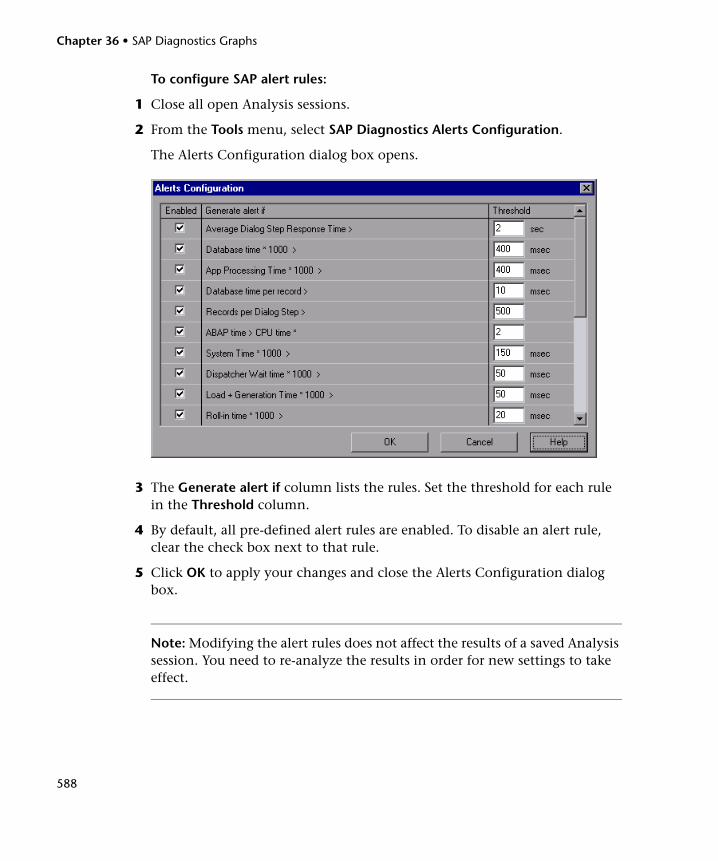
Chapter 36 • SAP Diagnostics Graphs
588
To configure SAP alert rules:
1 Close all open Analysis sessions.
2 From the Tools menu, select SAP Diagnostics Alerts Configuration.
The Alerts Configuration dialog box opens.
3 The Generate alert if column lists the rules. Set the threshold for each rule in the Threshold column.
4 By default, all pre-defined alert rules are enabled. To disable an alert rule, clear the check box next to that rule.
5 Click OK to apply your changes and close the Alerts Configuration dialog box.
Note: Modifying the alert rules does not affect the results of a saved Analysis session. You need to re-analyze the results in order for new settings to take effect.
Chapter 36 • SAP Diagnostics Graphs
589
Using the SAP Breakdown Options
The task pane is divided into 3 sections:
➤ The SAP Breakdown Toolbar
➤ Breakdown Options
➤ Filter and Grouping Options
The SAP Breakdown ToolbarThe toolbar contains the following buttons:
➤ Back. Click to view previous breakdown graph, or to ungroup grouped data.
➤ Next. Click to view next breakdown graph.
➤ Home. Click to return to the initial SAP Average Transaction Response Time graph.
➤ Help. Click to get help on the breakdown options.
Breakdown OptionsTo break down SAP diagnostics data, choose the breakdown and filter options from the task pane as follows:
➤ Break down transaction. Select a transaction from this list to display the average dialog step response time breakdown.
➤ Break down server time into. Displays the breakdown options for the Average Dialog Step Response Time Breakdown graph.
➤ Select Components to view a breakdown of the transaction’s server components, namely database time, interface time, application processing time, and system time.
➤ Select Dialog Steps to view a breakdown of the transaction’s dialog steps.
➤ Break down dialog step <dialog step>. Break down a dialog step into its server-time components, namely database time, interface time, application processing time, and system time.
Chapter 36 • SAP Diagnostics Graphs
590
➤ View data associated with <component>. Break down a server-time component (database time; interface time; application processing time; system time) to view data associated with it.
➤ No available breakdown. There are no further breakdown options.
➤ Apply. Click to apply the selected breakdown option.
Filter and Grouping OptionsThis section describes working with the filter settings and grouping options.
Current filter settings (non-edit mode)
This section displays the filter/grouping settings of the graph currently displayed in the primary graph pane.
➤ From/To. Display the time interval of the current graph.
➤ Transaction. Displays the name of the transaction represented in the graph.
➤ Dialog Step. Displays the name of the dialog step represented in the graph.
➤ Server. Displays the name of the server represented in the graph.
Edit Filter Settings
Click this button to modify filter or grouping settings. When you click Edit Filter Settings the filter/grouping options become editable.
➤ Filter. Use this option to filter the current graph by time interval, transaction, dialog step, and/or server.
➤ From/To. Enter values (in hh:mm:ss) to filter the graph over a specified time interval.
➤ By Transaction. Filter the graph to display information about a specific transaction by selecting the transaction from the list.
➤ By Dialog Step. Filter the graph to display information about a specific dialog step by selecting the dialog step from the list.
➤ By Server. Filter the graph to display information about a server by selecting the server name from the list.
Chapter 36 • SAP Diagnostics Graphs
591
Note: Only servers associated with the data displayed in the current graph are listed in the By Server list.
➤ Group. Use this option to group the data represented in the graph by transaction or by server. Select a transaction, component or subcomponent from the list.
➤ By Transaction. Select this check box to group by transaction.
➤ By Server. Select this check box to group by server.
Note: After applying grouping to a graph, you need to ungroup the data in order to apply further breakdown options. To ungroup grouped data, click the Back button on the toolbar.
IMPORTANT! When you open a saved session, the Back button is disabled. If you have grouped data, you need to click the Home button, or open a new SAP Diagnostics - Guided Flow tab to restart SAP breakdown.
➤ OK. Click OK to apply the chosen filter/grouping settings. The Current filter settings area displays the chosen settings in non-editable mode.
Notes:
➤ Global filtering is enabled when viewing SAP Diagnostics graphs (special SAP view) but cannot be applied on these graphs.
➤ Local filtering is disabled in the SAP Diagnostics - Guided Flow tab. To apply local filters to a SAP Diagnostics graph displayed in the Guided Flow tab, open the graph in a new tab by clicking the Enlarge Graph button.
Chapter 36 • SAP Diagnostics Graphs
592
Available SAP Diagnostics Graphs
You view the SAP Diagnostics graphs in the primary graph pane.
You can open these graphs in full view by clicking the Enlarge Graph button in the top right corner of the graph pane. An enlarged version of the graph opens in a new tab.
To filter or group data displayed in these graphs, see “Filter and Grouping Options” on page 590.
The available SAP Diagnostics graphs are:
➤ SAP Average Transaction Response Time Graph
➤ SAP Average Dialog Step Response Time Breakdown Graph
➤ SAP Server Time Breakdown (Dialog Steps) Graph
➤ SAP Server Time Breakdown Graph
➤ SAP Database Time Breakdown Graph
➤ SAP Application Processing Time Breakdown Graph
➤ SAP System Time Breakdown Graph
➤ SAP Interface Time Breakdown Graph
SAP Average Transaction Response Time GraphWhen you open the SAP Diagnostics - Guided Flow tab, the SAP Average Transaction Response Time graph opens in the primary graph pane, displaying all the SAP-related transactions in the load test scenario.
Note: Only transactions that are associated with SAP information are displayed in this graph.
For more information about the Average Transaction Response graph, see “Average Transaction Response Time Graph” on page 198.
Chapter 36 • SAP Diagnostics Graphs
593
To view the SAP breakdown of a specific transaction:
1 When the Average Transaction Breakdown graph is displayed in the primary graph pane, select a transaction in one of the following ways:
➤ Select the transaction from the Break down transaction: list in the task pane.
➤ Highlight the transaction by selecting the line representing it in the graph.
➤ Select the transaction from the graph legend. This highlights the line in the graph.
2 Click Apply in the task pane.
The SAP Average Dialog Step Response Time Breakdown graph opens in the primary graph pane. For more information, see “SAP Average Dialog Step Response Time Breakdown Graph” on page 594.
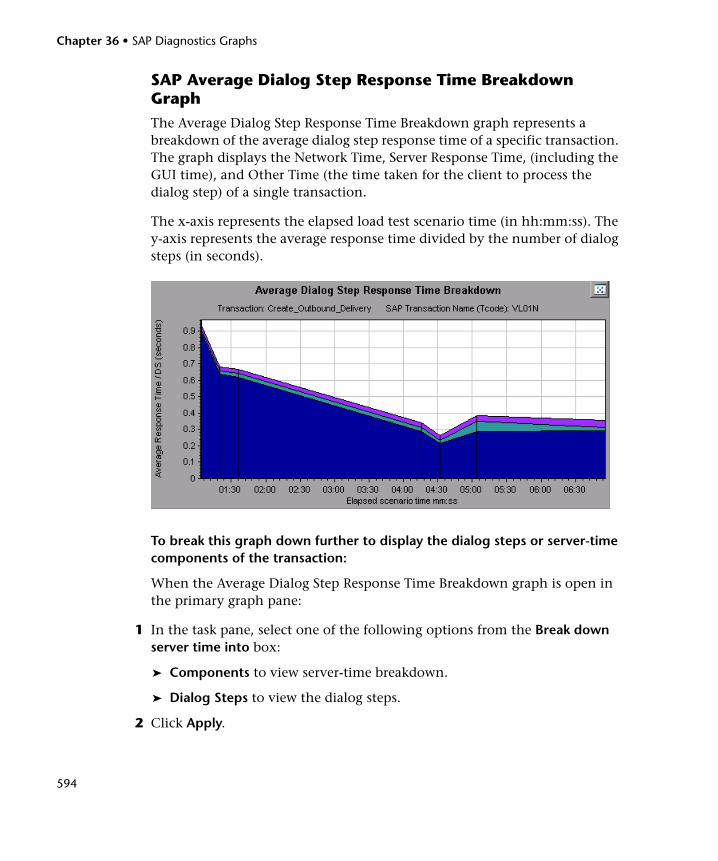
Chapter 36 • SAP Diagnostics Graphs
594
SAP Average Dialog Step Response Time Breakdown GraphThe Average Dialog Step Response Time Breakdown graph represents a breakdown of the average dialog step response time of a specific transaction. The graph displays the Network Time, Server Response Time, (including the GUI time), and Other Time (the time taken for the client to process the dialog step) of a single transaction.
The x-axis represents the elapsed load test scenario time (in hh:mm:ss). The y-axis represents the average response time divided by the number of dialog steps (in seconds).
To break this graph down further to display the dialog steps or server-time components of the transaction:
When the Average Dialog Step Response Time Breakdown graph is open in the primary graph pane:
1 In the task pane, select one of the following options from the Break down server time into box:
➤ Components to view server-time breakdown.
➤ Dialog Steps to view the dialog steps.
2 Click Apply.
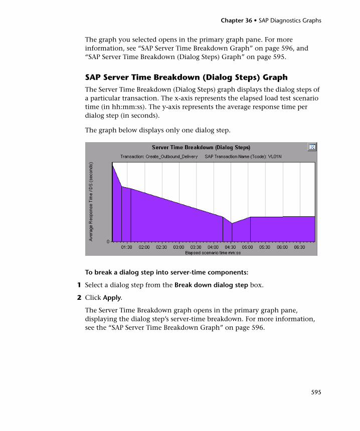
Chapter 36 • SAP Diagnostics Graphs
595
The graph you selected opens in the primary graph pane. For more information, see “SAP Server Time Breakdown Graph” on page 596, and “SAP Server Time Breakdown (Dialog Steps) Graph” on page 595.
SAP Server Time Breakdown (Dialog Steps) GraphThe Server Time Breakdown (Dialog Steps) graph displays the dialog steps of a particular transaction. The x-axis represents the elapsed load test scenario time (in hh:mm:ss). The y-axis represents the average response time per dialog step (in seconds).
The graph below displays only one dialog step.
To break a dialog step into server-time components:
1 Select a dialog step from the Break down dialog step box.
2 Click Apply.
The Server Time Breakdown graph opens in the primary graph pane, displaying the dialog step’s server-time breakdown. For more information, see the “SAP Server Time Breakdown Graph” on page 596.
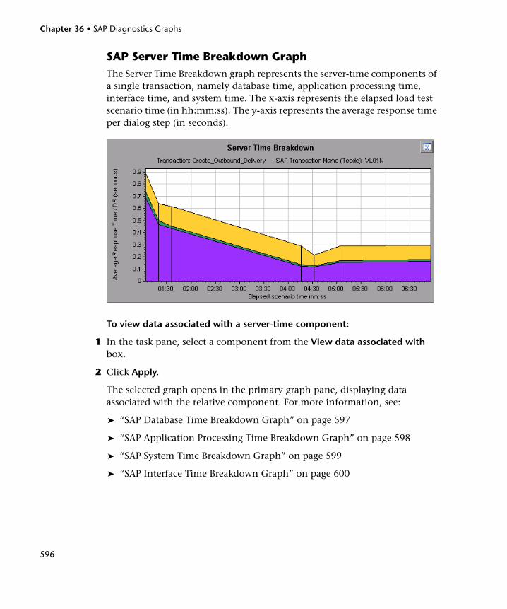
Chapter 36 • SAP Diagnostics Graphs
596
SAP Server Time Breakdown GraphThe Server Time Breakdown graph represents the server-time components of a single transaction, namely database time, application processing time, interface time, and system time. The x-axis represents the elapsed load test scenario time (in hh:mm:ss). The y-axis represents the average response time per dialog step (in seconds).
To view data associated with a server-time component:
1 In the task pane, select a component from the View data associated with box.
2 Click Apply.
The selected graph opens in the primary graph pane, displaying data associated with the relative component. For more information, see:
➤ “SAP Database Time Breakdown Graph” on page 597
➤ “SAP Application Processing Time Breakdown Graph” on page 598
➤ “SAP System Time Breakdown Graph” on page 599
➤ “SAP Interface Time Breakdown Graph” on page 600

Chapter 36 • SAP Diagnostics Graphs
597
SAP Database Time Breakdown GraphThe Database Time Breakdown graph displays the behavior of resources associated with database time, namely time taken to access a record, database time, and the number of records accessed per dialog step. The x-axis represents the elapsed load test scenario time (in hh:mm:ss). The y-axis represents the resource value per dialog step (in msec).
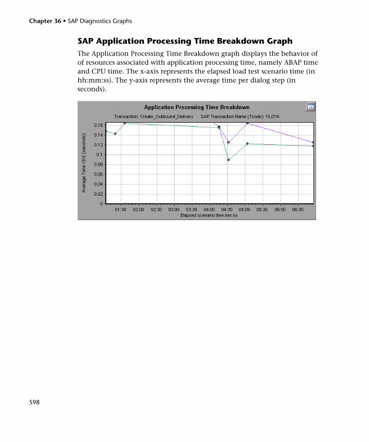
Chapter 36 • SAP Diagnostics Graphs
598
SAP Application Processing Time Breakdown GraphThe Application Processing Time Breakdown graph displays the behavior of of resources associated with application processing time, namely ABAP time and CPU time. The x-axis represents the elapsed load test scenario time (in hh:mm:ss). The y-axis represents the average time per dialog step (in seconds).
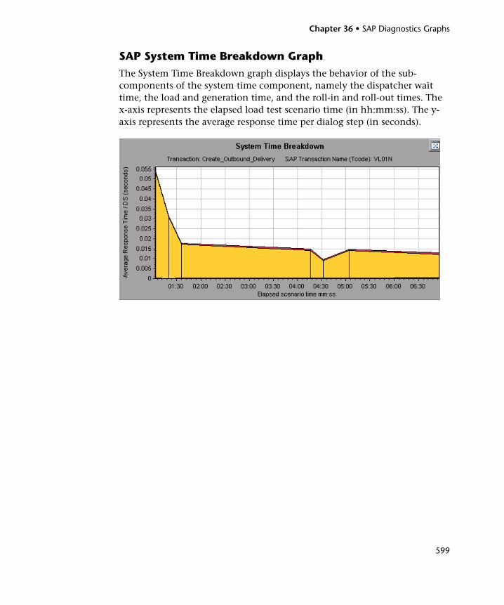
Chapter 36 • SAP Diagnostics Graphs
599
SAP System Time Breakdown GraphThe System Time Breakdown graph displays the behavior of the sub-components of the system time component, namely the dispatcher wait time, the load and generation time, and the roll-in and roll-out times. The x-axis represents the elapsed load test scenario time (in hh:mm:ss). The y-axis represents the average response time per dialog step (in seconds).
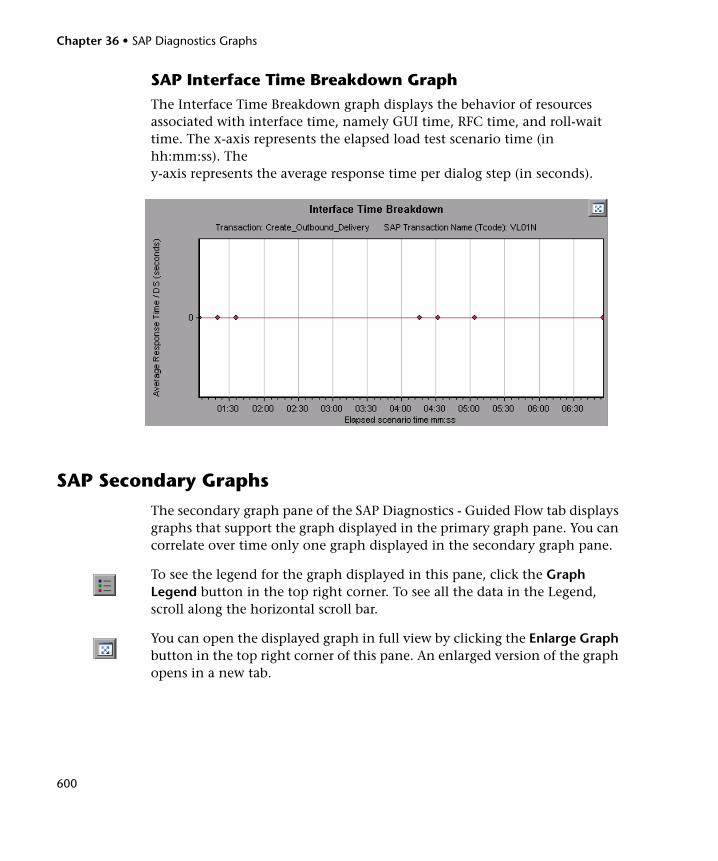
Chapter 36 • SAP Diagnostics Graphs
600
SAP Interface Time Breakdown GraphThe Interface Time Breakdown graph displays the behavior of resources associated with interface time, namely GUI time, RFC time, and roll-wait time. The x-axis represents the elapsed load test scenario time (in hh:mm:ss). The y-axis represents the average response time per dialog step (in seconds).
SAP Secondary Graphs
The secondary graph pane of the SAP Diagnostics - Guided Flow tab displays graphs that support the graph displayed in the primary graph pane. You can correlate over time only one graph displayed in the secondary graph pane.
To see the legend for the graph displayed in this pane, click the Graph Legend button in the top right corner. To see all the data in the Legend, scroll along the horizontal scroll bar.
You can open the displayed graph in full view by clicking the Enlarge Graph button in the top right corner of this pane. An enlarged version of the graph opens in a new tab.
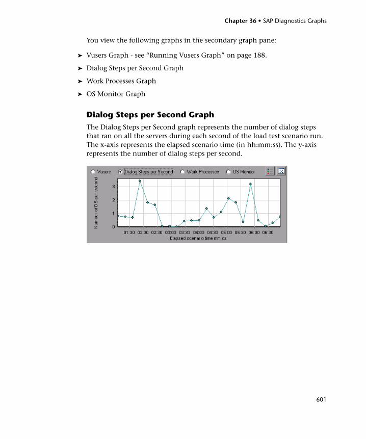
Chapter 36 • SAP Diagnostics Graphs
601
You view the following graphs in the secondary graph pane:
➤ Vusers Graph - see “Running Vusers Graph” on page 188.
➤ Dialog Steps per Second Graph
➤ Work Processes Graph
➤ OS Monitor Graph
Dialog Steps per Second GraphThe Dialog Steps per Second graph represents the number of dialog steps that ran on all the servers during each second of the load test scenario run. The x-axis represents the elapsed scenario time (in hh:mm:ss). The y-axis represents the number of dialog steps per second.
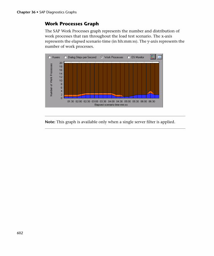
Chapter 36 • SAP Diagnostics Graphs
602
Work Processes GraphThe SAP Work Processes graph represents the number and distribution of work processes that ran throughout the load test scenario. The x-axis represents the elapsed scenario time (in hh:mm:ss). The y-axis represents the number of work processes.
Note: This graph is available only when a single server filter is applied.
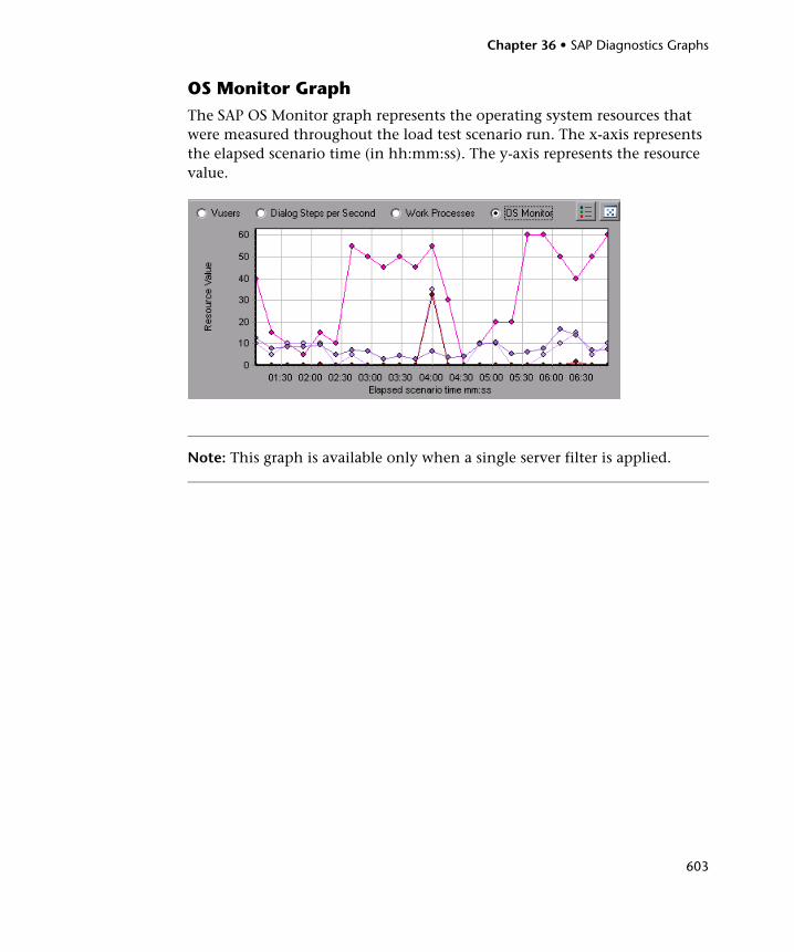
Chapter 36 • SAP Diagnostics Graphs
603
OS Monitor GraphThe SAP OS Monitor graph represents the operating system resources that were measured throughout the load test scenario run. The x-axis represents the elapsed scenario time (in hh:mm:ss). The y-axis represents the resource value.
Note: This graph is available only when a single server filter is applied.

Chapter 36 • SAP Diagnostics Graphs
604
605
37J2EE & .NET Diagnostics Graphs
After a load test scenario run, you can use LoadRunner Analysis to display the J2EE & .NET Diagnostics graphs to analyze server performance.
This chapter includes:
➤ About J2EE & .NET Diagnostics Graphs on page 606
➤ Enabling Diagnostics for J2EE & .NET on page 606
➤ Viewing J2EE & .NET Diagnostics in the Summary Report on page 607
➤ Viewing J2EE & .NET Diagnostics Data on page 609
➤ J2EE & .NET Diagnostics Graphs on page 626
➤ J2EE & .NET Server Diagnostics Graphs on page 636
Chapter 37 • J2EE & .NET Diagnostics Graphs
606
About J2EE & .NET Diagnostics Graphs
The J2EE & .NET Diagnostics graphs in LoadRunner Analysis enable you to trace, time, and troubleshoot individual transactions and server requests through J2EE & .NET Web, application, and database servers. You can also quickly pinpoint problem servlets and JDBC calls to maximize business process performance, scalability, and efficiency.
The J2EE & .NET Diagnostics graphs are comprised of two groups:
➤ J2EE & .NET Diagnostics Graphs. These graphs show you the performance of requests and methods generated by virtual user transactions. They show you the transaction that generated each request.
➤ J2EE & .NET Server Diagnostics Graphs. These graphs show you the performance of all the requests and methods in the application you are monitoring. These include requests generated by virtual user transactions and by real users.
Enabling Diagnostics for J2EE & .NET
To generate Diagnostics for J2EE & .NET data, you must first install HP Diagnostics.
Before you can use HP Diagnostics with LoadRunner, you need to ensure that you have specified the Diagnostics Server details in LoadRunner. Before you can view Diagnostics for J2EE & .NET data in a particular load test scenario, you need to configure the Diagnostics parameters for that scenario. For more information about Configuring HP Diagnostics to work with LoadRunner, refer to the HP LoadRunner Controller User Guide.
Important: To ensure that valid J2EE/.NET diagnostics data is generated during the scenario run, you must manually mark the beginning and end of each transaction in the Vuser script, rather than using automatic transactions.
Chapter 37 • J2EE & .NET Diagnostics Graphs
607
Viewing J2EE & .NET Diagnostics in the Summary Report
The J2EE & .NET Diagnostics Usage section of the Summary report provides general information about load test scenario execution and a usage chart for the J2EE & .NET Diagnostics and server request layers. This report is available from the Session Explorer or as a tab in the Analysis window.
Note: If you do not see diagnostics data on the Summary Report, check if you are using a user-defined template. To view relevant data, choose a different template from the list of templates, or create and apply a new template. For more information about using templates, see “Using Templates” on page 76.
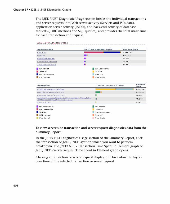
Chapter 37 • J2EE & .NET Diagnostics Graphs
608
The J2EE /.NET Diagnostic Usage section breaks the individual transactions and server requests into Web server activity (Servlets and JSPs data), application server activity (JNDIs), and back-end activity of database requests (JDBC methods and SQL queries), and provides the total usage time for each transaction and request.
To view server side transaction and server request diagnostics data from the Summary Report:
In the J2EE/.NET Diagnostics Usage section of the Summary Report, click the transaction or J2EE /.NET layer on which you want to perform breakdown. The J2EE/.NET - Transaction Time Spent in Element graph or J2EE/.NET - Server Request Time Spent in Element graph opens.
Clicking a transaction or server request displays the breakdown to layers over time of the selected transaction or server request.
Chapter 37 • J2EE & .NET Diagnostics Graphs
609
Clicking a layer displays the specific layer breakdown in the transaction or server request. For more information, see “J2EE/.NET - Transaction Time Spent in Element Graph” on page 630 and “J2EE/.NET - Server Request Time Spent in Element Graph” on page 640.
For more information on J2EE/.NET Diagnostics graphs, see “Viewing J2EE & .NET Diagnostics Data” below.
Viewing J2EE & .NET Diagnostics Data
The J2EE & .NET Diagnostics graphs provide an overview of the entire chain of activity on the server side of the system. At the same time, you can break down J2EE/.NET layers into classes and methods to enable you to pinpoint the exact location where time is consumed. In addition, you can view custom classes or packages that you set the J2EE/.NET probe to monitor. You can also view the transaction chain of calls and call stack statistics to track the percentage of time spent on each part of the transaction.
You can correlate the end user response time with the Web server activity (Servlets and JSPs data), application server activity (JNDIs), and back-end activity of database requests (JDBC methods and SQL queries).
Example Transaction BreakdownThe following graphs illustrate the breakdown of a transaction to its layers, classes, and methods.
Chapter 37 • J2EE & .NET Diagnostics Graphs
610
Transaction Level
The following figure displays the top level Average Transaction Response Time graph. The graph displays several transactions: Birds, Bulldog, Checkout, Start, etc.
Chapter 37 • J2EE & .NET Diagnostics Graphs
611
Layer Level
In the following figure, the Start transaction has been broken down to its layers (DB, EJB, JNDI, and Web). In J2EE/.NET transactions, the Web layer is generally the largest.
Chapter 37 • J2EE & .NET Diagnostics Graphs
612
Class Level
In the following figure, the Web layer of the Start transaction has been broken down to its classes.
Chapter 37 • J2EE & .NET Diagnostics Graphs
613
Method/Query Level
In the following figure, the weblogic.servlet.FileServlet component of the Web layer of the Start transaction has been broken down to its methods.
Note: Some JDBC methods can invoke SQLs which can be broken down further. In this case there is another level of breakdown, that is SQL Statements. For the methods that can not be further broken down into SQL statements when reaching this level of breakdown, you see NoSql.
Chapter 37 • J2EE & .NET Diagnostics Graphs
614
Cross VM Analysis
When a server request makes a remote method invocation, the J2EE & .NET Diagnostics graphs display certain measurements relating to the classes and methods involved in these requests. These measurements are displayed at a layer, class and method level. The VM making the call is referred to as the caller VM, and the VM that executes the remote call is the callee VM.
Cross VM Layer is a measurement that represents a dummy layer that integrates the data from the remote classes and methods in server requests that take place across two or more virtual machines.
Remote-Class is a measurement that represents a dummy class that integrates the data from the remote methods in server requests that take place across two or more virtual machines.
Remote-Class: Remote Method is a measurement that represents a dummy method. Remote-Class: Remote Method measures the total time, call count, exclusive latency, minimum and maximum values, standard deviation, and so on of the methods that are executed remotely, relative to the caller virtual machine.
Note: Since this data is measured on the caller virtual machine the exclusive latency will include all of the time required for making the remote method invocation such as network latency.
Chapter 37 • J2EE & .NET Diagnostics Graphs
615
Using the J2EE & .NET Breakdown OptionsYou can activate the J2EE & .NET breakdown options in any one of the following ways:
➤ from the View menu
➤ by right-clicking on a transaction or server request and choosing the option from the short-cut menu
➤ by clicking the button in the toolbar above the graph
Note: The breakdown menu options and buttons are not displayed until an element (transaction, server request, layer) is selected.
To view server side diagnostics data:
1 From the Average Response Time graph, right-click a transaction line and choose J2EE/.NET Diagnostics > Show Server Requests, or choose View > J2EE/.NET Diagnostics > Show Server Requests. Alternatively, click the Show Server Requests button in the toolbar above the graph.
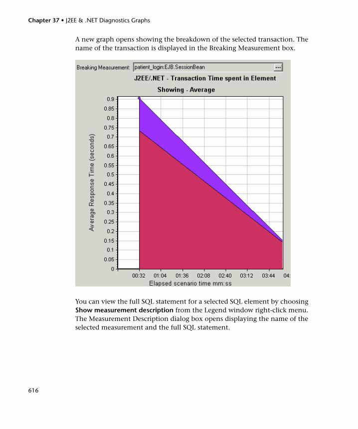
Chapter 37 • J2EE & .NET Diagnostics Graphs
616
A new graph opens showing the breakdown of the selected transaction. The name of the transaction is displayed in the Breaking Measurement box.
You can view the full SQL statement for a selected SQL element by choosing Show measurement description from the Legend window right-click menu. The Measurement Description dialog box opens displaying the name of the selected measurement and the full SQL statement.
Chapter 37 • J2EE & .NET Diagnostics Graphs
617
Note: If there is no URI in the SQL, URI-None appears in front of the full measurement description in the Measurement Description dialog box.
To view transaction properties for the breakdown measurement, click the Breaking Measurement button. To disable this feature, choose View > Display Options, and clear the Show Breaking Measurement check box.
2 At this point, you can select a displayed element and use the J2EE/.NET Diagnostics menu or buttons to do the following:
➤ Break the data down to a lower level by doing one of the following:
➤ Select View > J2EE/.NET Diagnostics > Break down the server request to layers, or click the measurement breakdownbutton in the toolbar above the graph.
Note: The option in the J2EE/.NET Diagnostics menu, and the tool tip of the measurement breakdown button, vary according to the element that you want to break down. For example, when you select a server request, the menu option and tool tip are Break down server request to layers.
➤ Select View > J2EE/.NET Diagnostics > Show VM, or click the Show VM button in the toolbar above the graph. This breaks the data down to the application host name (VM).
Chapter 37 • J2EE & .NET Diagnostics Graphs
618
➤ Return to a previous level by doing one of the following:
➤ Select View > J2EE/.NET Diagnostics > Undo Break down the server request to layers, or click the Undo <Measurement Breakdown>button in the toolbar above the graph.
Note: The option in the J2EE/.NET Diagnostics menu, and the tool tip of the measurement breakdown button, vary according to the element whose breakdown you want to undo. For example, when you select a layer, the menu option and tool tip are Undo break down server request to layers.
➤ Select View > J2EE/.NET Diagnostics > Hide VM, or click the Hide VM button in the toolbar above the graph.
➤ Display the chain of call or call stack statistics in the measurements tree window: Drag the orange time line on to the graph to the time specifying the end of the period for which you want to view data, and choose View > J2EE/.NET Diagnostics > Show Chain of Calls, or click the Show Chain of Calls button in the toolbar above the graph.
Note: A measurement that is broken down in the Average Method Response Time in Transactions graph will be different from the same measurement broken down in the J2EE/.NET - Transaction Time Spent in Element graph. This is because the J2EE/.NET - Average Method Response Time in Transactions graph displays the average transaction time, whereas the J2EE/.NET - Transaction Time Spent in Element graph displays the average time per transaction event (sum of method execution time).
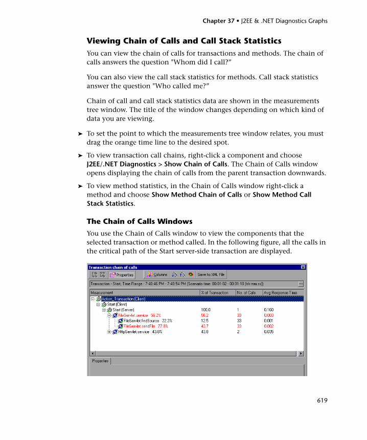
Chapter 37 • J2EE & .NET Diagnostics Graphs
619
Viewing Chain of Calls and Call Stack StatisticsYou can view the chain of calls for transactions and methods. The chain of calls answers the question "Whom did I call?”
You can also view the call stack statistics for methods. Call stack statistics answer the question "Who called me?”
Chain of call and call stack statistics data are shown in the measurements tree window. The title of the window changes depending on which kind of data you are viewing.
➤ To set the point to which the measurements tree window relates, you must drag the orange time line to the desired spot.
➤ To view transaction call chains, right-click a component and choose J2EE/.NET Diagnostics > Show Chain of Calls. The Chain of Calls window opens displaying the chain of calls from the parent transaction downwards.
➤ To view method statistics, in the Chain of Calls window right-click a method and choose Show Method Chain of Calls or Show Method Call Stack Statistics.
The Chain of Calls Windows
You use the Chain of Calls window to view the components that the selected transaction or method called. In the following figure, all the calls in the critical path of the Start server-side transaction are displayed.
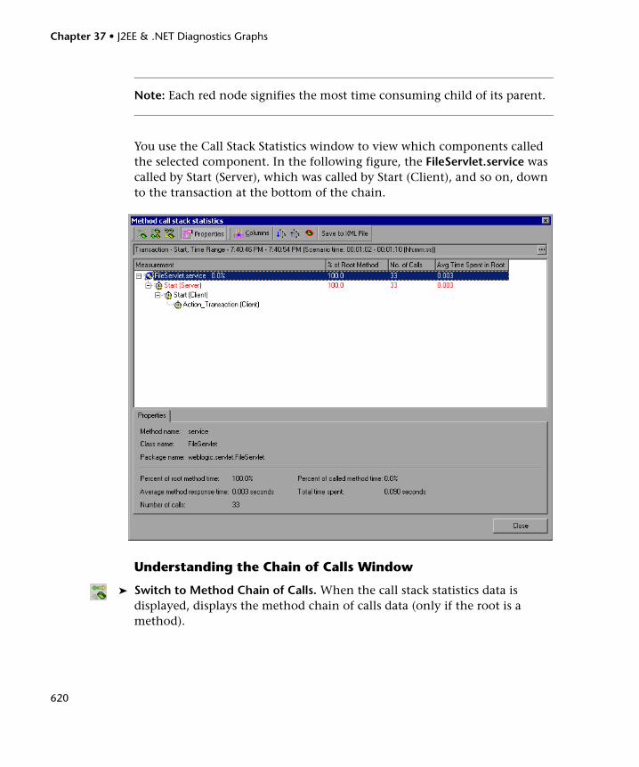
Chapter 37 • J2EE & .NET Diagnostics Graphs
620
Note: Each red node signifies the most time consuming child of its parent.
You use the Call Stack Statistics window to view which components called the selected component. In the following figure, the FileServlet.service was called by Start (Server), which was called by Start (Client), and so on, down to the transaction at the bottom of the chain.
Understanding the Chain of Calls Window
➤ Switch to Method Chain of Calls. When the call stack statistics data is displayed, displays the method chain of calls data (only if the root is a method).
Chapter 37 • J2EE & .NET Diagnostics Graphs
621
➤ Switch to Method Call Stack Statistics. When the method chain of calls data is displayed, displays the method call stack statistics data (only if the root is a method).
➤ Show Method Chain of Calls. Displays the Chain of Calls window.
➤ Show Method Call Stack Statistics. Displays the Call Stack Statistics window.
➤ Properties. Hides or displays the properties area (lower pane).
➤ Columns. Enables you to select the columns shown in the Calls window. To display additional fields, drag them to the desired location in the Calls window. To remove fields, drag them from the Calls window back to the Columns chooser.
The following columns are available in the Chain of Calls window:
Column Description
Measurement Name of the method, displayed as ComponentName:MethodName. In the case of a database call, query information is also displayed. The percent shown indicates the percentage of calls to this component from its parent.
% of Root Method Percentage of the total time of the method from the total time of the root tree item.
No of Calls Displays the amount of times this transaction or method was executed.
Avg Response Time Response time is the time from the beginning of execution until the end. Average response time is the total response time divided by the number of divided by the number of instances of the method.
STD Response Time The standard deviation response time.
Min Response Time The minimum response time.
Max Response Time The maximum response time.
% of Caller Displays the percentage of method time in relation the parent method time.
Total time Displays the total method execution time, including the child execution time.
Chapter 37 • J2EE & .NET Diagnostics Graphs
622
The following columns are available in the Call Stack Statistics window:
➤ Expand All. Expands the entire tree.
➤ Collapse All. Collapses the entire tree.
➤ Expand Worst Path. Expands only the parts of the path on the critical path.
➤ Save to XML File. Saves the tree data to an XML file.
➤ Method Properties Area. Displays the full properties of the selected method.
➤ SQL Query. Displays the SQL query for the selected method. (For Database only.)
Column Description
Measurement Name of the method, displayed as ComponentName.MethodName. In the case of a database call, query information is also displayed. The percent shown indicates the percentage of calls to this component from its child.
% of Root Method Percentage of the total time of the transaction (or method) from the total time of the root tree item.
No. of Calls to Root Displays the amount of times this transaction or method was executed.
Avg Time Spent in Root Time spent in root is the time that the sub-area spent in the root sub-area/area/transaction.
Average Time Spent in Root time is the total time spent in the root divided by the number of instances of the method.
STD Time Spent in Root The standard deviation time spent in the root.
Min Time Spent in Root The minimum time spent in the root.
Max Time Spent in Root The maximum time spent in the root.
% of Called Displays the percentage o method time in relation the child method time.
Total Time Spent in Root Displays the total method execution time, including the child execution time.
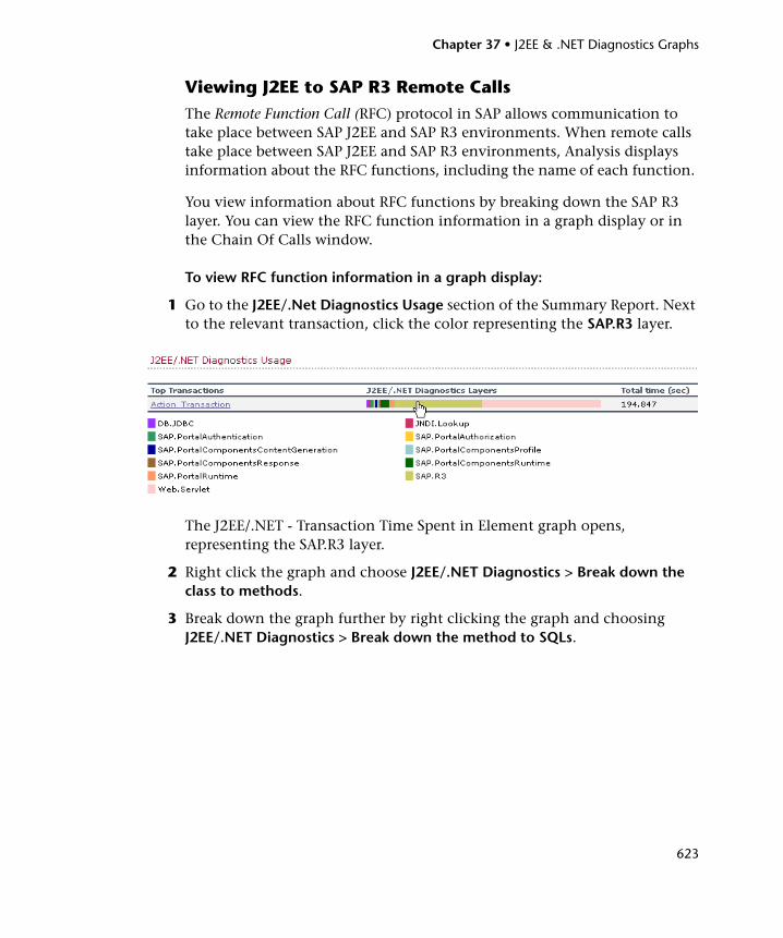
Chapter 37 • J2EE & .NET Diagnostics Graphs
623
Viewing J2EE to SAP R3 Remote CallsThe Remote Function Call (RFC) protocol in SAP allows communication to take place between SAP J2EE and SAP R3 environments. When remote calls take place between SAP J2EE and SAP R3 environments, Analysis displays information about the RFC functions, including the name of each function.
You view information about RFC functions by breaking down the SAP R3 layer. You can view the RFC function information in a graph display or in the Chain Of Calls window.
To view RFC function information in a graph display:
1 Go to the J2EE/.Net Diagnostics Usage section of the Summary Report. Next to the relevant transaction, click the color representing the SAP.R3 layer.
The J2EE/.NET - Transaction Time Spent in Element graph opens, representing the SAP.R3 layer.
2 Right click the graph and choose J2EE/.NET Diagnostics > Break down the class to methods.
3 Break down the graph further by right clicking the graph and choosing J2EE/.NET Diagnostics > Break down the method to SQLs.
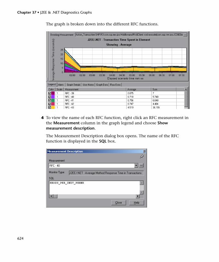
Chapter 37 • J2EE & .NET Diagnostics Graphs
624
The graph is broken down into the different RFC functions.
4 To view the name of each RFC function, right click an RFC measurement in the Measurement column in the graph legend and choose Show measurement description.
The Measurement Description dialog box opens. The name of the RFC function is displayed in the SQL box.
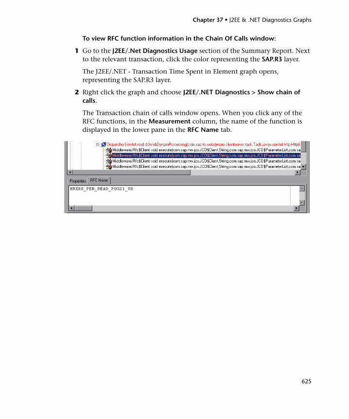
Chapter 37 • J2EE & .NET Diagnostics Graphs
625
To view RFC function information in the Chain Of Calls window:
1 Go to the J2EE/.Net Diagnostics Usage section of the Summary Report. Next to the relevant transaction, click the color representing the SAP.R3 layer.
The J2EE/.NET - Transaction Time Spent in Element graph opens, representing the SAP.R3 layer.
2 Right click the graph and choose J2EE/.NET Diagnostics > Show chain of calls.
The Transaction chain of calls window opens. When you click any of the RFC functions, in the Measurement column, the name of the function is displayed in the lower pane in the RFC Name tab.
Chapter 37 • J2EE & .NET Diagnostics Graphs
626
J2EE & .NET Diagnostics Graphs
This section includes:
➤ “Setting Graph Filter Properties” on page 626
➤ “J2EE/.NET - Transaction Response Time Server Side Graph” on page 628
➤ “J2EE/.NET - Average Method Response Time in Transactions Graph” on page 629
➤ “J2EE/.NET - Transaction Time Spent in Element Graph” on page 630
➤ “J2EE/.NET - Transactions per Second Graph” on page 632
➤ “J2EE/.NET - Method Calls per Second in Transactions Graph” on page 633
➤ “J2EE/.NET - Average Number of Exceptions in Transactions Graph” on page 634
➤ “J2EE/.NET - Average Number of Timeouts in Transactions Graph” on page 635
Note: To generate Diagnostics for J2EE & .NET data, you must first install HP Diagnostics. Before you can view Diagnostics for J2EE & .NET data in a particular load test scenario, you need to configure the Diagnostics parameters for that scenario, as described in the HP LoadRunner Controller User Guide.
Setting Graph Filter PropertiesYou can filter the J2EE & .NET Diagnostics graphs so that the displayed data is more suitable to your needs. You can filter using the following methods:
➤ Before opening a graph, enter filter criteria in the Graph Properties box of the Open Graph dialog box. For more information, see “Accessing and Opening Graphs and Reports” on page 30.
➤ From an open graph, enter filter criteria in the Filter condition fields in a filter dialog box. For more information, see “Filtering and Sorting Graph Data” on page 79 and “Drilling Down in a Graph” on page 102.
Chapter 37 • J2EE & .NET Diagnostics Graphs
627
You can filter the J2EE & .NET Diagnostics graphs by the following fields:
➤ Scenario Elapsed Time. Shows data for transactions that ended during the specified time.
➤ Transaction Name - J2EE/.NET. Shows data for a specified transaction.
➤ Layer Name. Shows data for specified layers.
➤ Class Name. Shows data for specified classes.
➤ SQL Logical Name. Shows data for specified SQL logical names. Due to the length of some SQL names, after you choose an SQL statement it is assigned a "logical name." This logical name is used in the filter dialog, legend, grouping, and other places in place of the full SQL statement. You can view the full SQL statement in the Measurement Description dialog box (View > Show Measurement Description).
Some JDBC methods have the ability to invoke SQL’s (each method can invoke several different SQL’s) so there is another level of breakdown which is the SQL statements.
Note: For the methods that do not have SQL statement when reaching this level of breakdown you see NoSql.
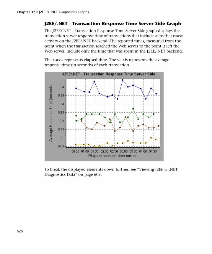
Chapter 37 • J2EE & .NET Diagnostics Graphs
628
J2EE/.NET - Transaction Response Time Server Side GraphThe J2EE/.NET - Transaction Response Time Server Side graph displays the transaction server response time of transactions that include steps that cause activity on the J2EE/.NET backend. The reported times, measured from the point when the transaction reached the Web server to the point it left the Web server, include only the time that was spent in the J2EE/.NET backend.
The x-axis represents elapsed time. The y-axis represents the average response time (in seconds) of each transaction.
To break the displayed elements down further, see “Viewing J2EE & .NET Diagnostics Data” on page 609.
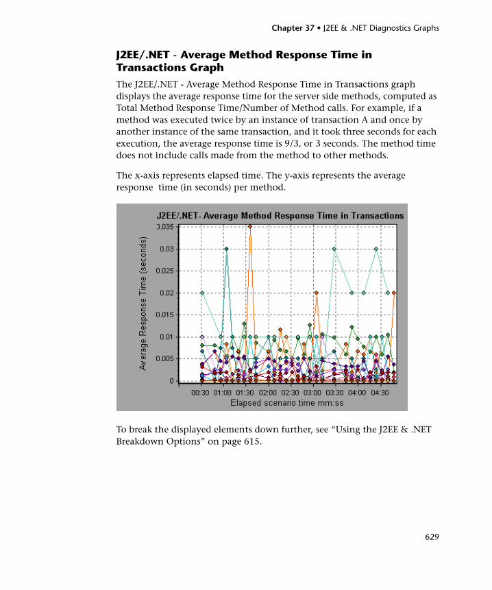
Chapter 37 • J2EE & .NET Diagnostics Graphs
629
J2EE/.NET - Average Method Response Time in Transactions GraphThe J2EE/.NET - Average Method Response Time in Transactions graph displays the average response time for the server side methods, computed as Total Method Response Time/Number of Method calls. For example, if a method was executed twice by an instance of transaction A and once by another instance of the same transaction, and it took three seconds for each execution, the average response time is 9/3, or 3 seconds. The method time does not include calls made from the method to other methods.
The x-axis represents elapsed time. The y-axis represents the average response time (in seconds) per method.
To break the displayed elements down further, see “Using the J2EE & .NET Breakdown Options” on page 615.
Chapter 37 • J2EE & .NET Diagnostics Graphs
630
J2EE/.NET - Transaction Time Spent in Element GraphThe J2EE/.NET - Transaction Time Spent in Element graph displays the server response time for the selected element (layer, class, or method) within each transaction.
The display of graph data is determined by the graph properties selected when the graph was opened, as described in the following table:
For more information on filtering by graph properties, see “Setting Graph Filter Properties” on page 626.
The time is computed as Total Response Time/Total Number of Transactions. For example, if a method was executed twice by an instance of transaction A and once by another instance of the same transaction, and it took three seconds for each execution, the average response time is 9/2, or 4.5 seconds. The transaction time does not include the nested calls from within each transaction.
If you filter by these properties...
The graph data is displayed like this
None Time spent in each transaction.
Transaction Filtered by transaction. Grouped by layer.
Transaction and layer Filtered by transaction and layer. Grouped by class.
Transaction, layer, and class
Filtered by transaction, layer, and class. Grouped by method.
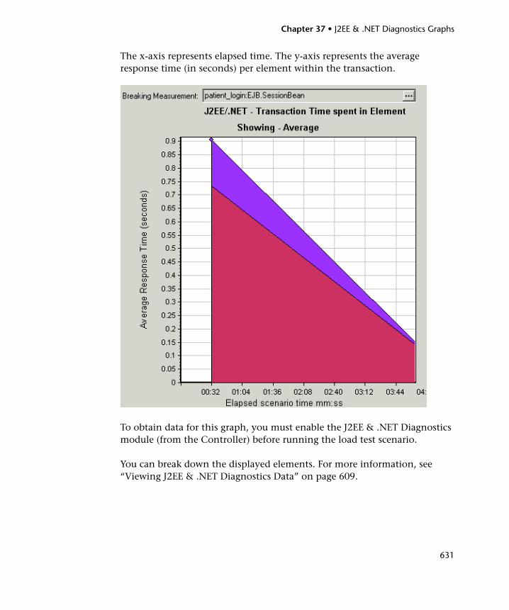
Chapter 37 • J2EE & .NET Diagnostics Graphs
631
The x-axis represents elapsed time. The y-axis represents the average response time (in seconds) per element within the transaction.
To obtain data for this graph, you must enable the J2EE & .NET Diagnostics module (from the Controller) before running the load test scenario.
You can break down the displayed elements. For more information, see “Viewing J2EE & .NET Diagnostics Data” on page 609.
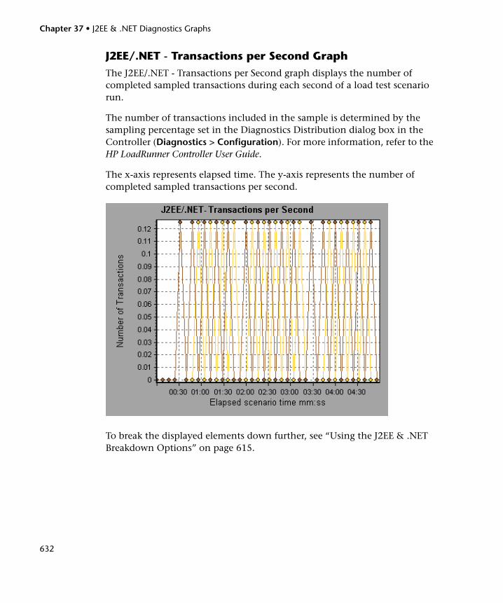
Chapter 37 • J2EE & .NET Diagnostics Graphs
632
J2EE/.NET - Transactions per Second GraphThe J2EE/.NET - Transactions per Second graph displays the number of completed sampled transactions during each second of a load test scenario run.
The number of transactions included in the sample is determined by the sampling percentage set in the Diagnostics Distribution dialog box in the Controller (Diagnostics > Configuration). For more information, refer to the HP LoadRunner Controller User Guide.
The x-axis represents elapsed time. The y-axis represents the number of completed sampled transactions per second.
To break the displayed elements down further, see “Using the J2EE & .NET Breakdown Options” on page 615.
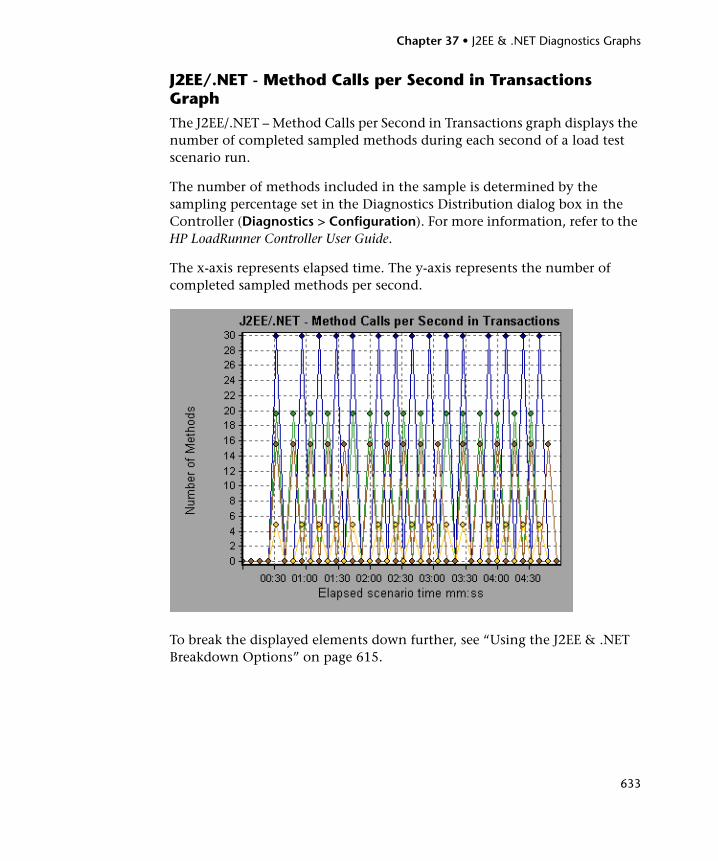
Chapter 37 • J2EE & .NET Diagnostics Graphs
633
J2EE/.NET - Method Calls per Second in Transactions GraphThe J2EE/.NET – Method Calls per Second in Transactions graph displays the number of completed sampled methods during each second of a load test scenario run.
The number of methods included in the sample is determined by the sampling percentage set in the Diagnostics Distribution dialog box in the Controller (Diagnostics > Configuration). For more information, refer to the HP LoadRunner Controller User Guide.
The x-axis represents elapsed time. The y-axis represents the number of completed sampled methods per second.
To break the displayed elements down further, see “Using the J2EE & .NET Breakdown Options” on page 615.
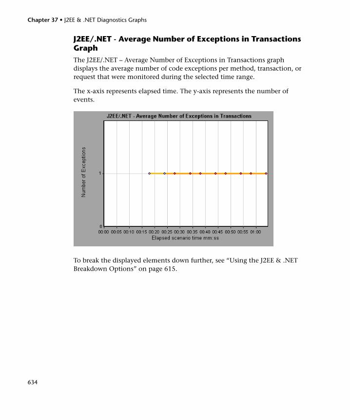
Chapter 37 • J2EE & .NET Diagnostics Graphs
634
J2EE/.NET - Average Number of Exceptions in Transactions GraphThe J2EE/.NET – Average Number of Exceptions in Transactions graph displays the average number of code exceptions per method, transaction, or request that were monitored during the selected time range.
The x-axis represents elapsed time. The y-axis represents the number of events.
To break the displayed elements down further, see “Using the J2EE & .NET Breakdown Options” on page 615.
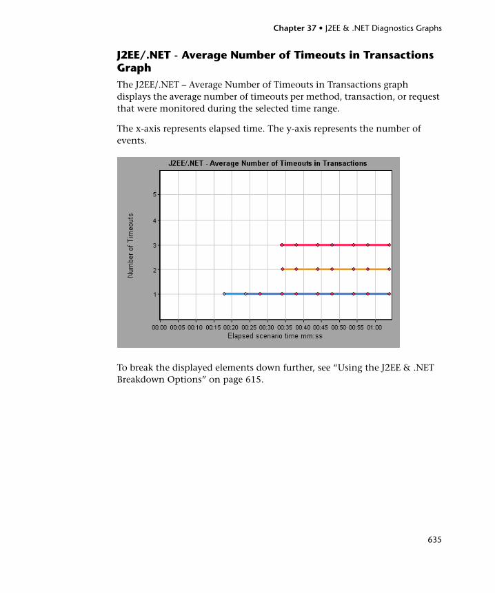
Chapter 37 • J2EE & .NET Diagnostics Graphs
635
J2EE/.NET - Average Number of Timeouts in Transactions GraphThe J2EE/.NET – Average Number of Timeouts in Transactions graph displays the average number of timeouts per method, transaction, or request that were monitored during the selected time range.
The x-axis represents elapsed time. The y-axis represents the number of events.
To break the displayed elements down further, see “Using the J2EE & .NET Breakdown Options” on page 615.
Chapter 37 • J2EE & .NET Diagnostics Graphs
636
J2EE & .NET Server Diagnostics Graphs
This section includes:
➤ “Setting Graph Filter Properties” on page 636
➤ “J2EE/.NET - Server Request Response Time Graph” on page 638
➤ “J2EE/.NET - Average Server Method Response Time Graph” on page 639
➤ “J2EE/.NET - Server Request Time Spent in Element Graph” on page 640
➤ “J2EE/.NET - Server Requests per Second Graph” on page 642
➤ “J2EE/.NET - Server Methods Calls per Second Graph” on page 643
➤ “J2EE/.NET - Average Number of Exceptions on Server Graph” on page 644
➤ “J2EE/.NET - Average Number of Timeouts on Server Graph” on page 645
Note: To generate Diagnostics for J2EE & .NET data, you must first install HP Diagnostics. Before you can view Diagnostics for J2EE & .NET data in a particular load test scenario, you need to configure the Diagnostics parameters for that scenario, as described in the HP LoadRunner Controller User Guide.
Setting Graph Filter PropertiesYou can filter the J2EE/.NET Server Diagnostics graphs so that the displayed data is more suitable to your needs. You can filter using the following methods:
➤ Before opening a graph, enter filter criteria in the Graph Properties box of the Open Graph dialog box. For more information, see “Accessing and Opening Graphs and Reports” on page 30.
➤ From an open graph, enter filter criteria in the Filter condition fields in a filter dialog box. For more information, see “Filtering and Sorting Graph Data” on page 79.
Chapter 37 • J2EE & .NET Diagnostics Graphs
637
You can filter the J2EE/.NET Server Diagnostics graphs by the following fields:
➤ Scenario Elapsed Time. Shows data for requests that ended during the specified time.
➤ Server Request. Shows data for a specified request.
➤ Layer Name. Shows data for specified layers.
➤ Class Name. Shows data for specified classes.
➤ SQL Logical Name. Shows data for specified SQL logical names. Due to the length of some SQL names, after you choose an SQL statement it is assigned a "logical name."This logical name is used in the filter dialog, legend, grouping, and other places in place of the full SQL statement. You can view the full SQL statement in the Measurement Description dialog box (View > Show Measurement Description).
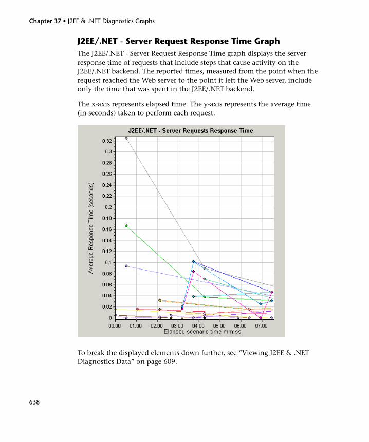
Chapter 37 • J2EE & .NET Diagnostics Graphs
638
J2EE/.NET - Server Request Response Time GraphThe J2EE/.NET - Server Request Response Time graph displays the server response time of requests that include steps that cause activity on the J2EE/.NET backend. The reported times, measured from the point when the request reached the Web server to the point it left the Web server, include only the time that was spent in the J2EE/.NET backend.
The x-axis represents elapsed time. The y-axis represents the average time (in seconds) taken to perform each request.
To break the displayed elements down further, see “Viewing J2EE & .NET Diagnostics Data” on page 609.
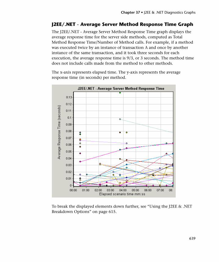
Chapter 37 • J2EE & .NET Diagnostics Graphs
639
J2EE/.NET - Average Server Method Response Time GraphThe J2EE/.NET - Average Server Method Response Time graph displays the average response time for the server side methods, computed as Total Method Response Time/Number of Method calls. For example, if a method was executed twice by an instance of transaction A and once by another instance of the same transaction, and it took three seconds for each execution, the average response time is 9/3, or 3 seconds. The method time does not include calls made from the method to other methods.
The x-axis represents elapsed time. The y-axis represents the average response time (in seconds) per method.
To break the displayed elements down further, see “Using the J2EE & .NET Breakdown Options” on page 615.
Chapter 37 • J2EE & .NET Diagnostics Graphs
640
J2EE/.NET - Server Request Time Spent in Element GraphThe J2EE/.NET - Server Request Time Spent in Element graph displays the server response time for the selected element (layer, class, or method) within each server request.
The display of graph data is determined by the Graph Properties selected when the graph was opened, as described in the following table:
For more information on filtering by graph properties, see “Setting Graph Filter Properties” on page 626.
The time is computed as Total Response Time/Total Number of Server Requests. For example, if a method was executed twice by an instance of server request A and once by another instance of the same server request, and it took three seconds for each execution, the average response time is 9/2, or 4.5 seconds. The server request time does not include the nested calls from within each server request.
If you filter by these properties
The graph data is displayed like this
None Time spent in each server request.
Server request. Filtered by server request. Grouped by layer.
Server request and layer Filtered by server request and layer. Grouped by class.
Server request, layer, and class
Filtered by server request, layer, and class. Grouped by method.
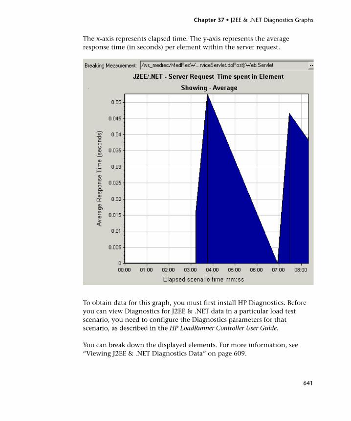
Chapter 37 • J2EE & .NET Diagnostics Graphs
641
The x-axis represents elapsed time. The y-axis represents the average response time (in seconds) per element within the server request.
To obtain data for this graph, you must first install HP Diagnostics. Before you can view Diagnostics for J2EE & .NET data in a particular load test scenario, you need to configure the Diagnostics parameters for that scenario, as described in the HP LoadRunner Controller User Guide.
You can break down the displayed elements. For more information, see “Viewing J2EE & .NET Diagnostics Data” on page 609.
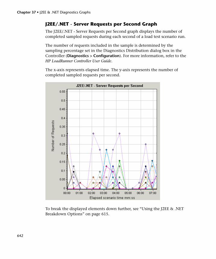
Chapter 37 • J2EE & .NET Diagnostics Graphs
642
J2EE/.NET - Server Requests per Second GraphThe J2EE/.NET - Server Requests per Second graph displays the number of completed sampled requests during each second of a load test scenario run.
The number of requests included in the sample is determined by the sampling percentage set in the Diagnostics Distribution dialog box in the Controller (Diagnostics > Configuration). For more information, refer to the HP LoadRunner Controller User Guide.
The x-axis represents elapsed time. The y-axis represents the number of completed sampled requests per second.
To break the displayed elements down further, see “Using the J2EE & .NET Breakdown Options” on page 615.
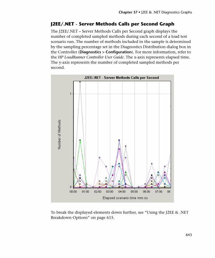
Chapter 37 • J2EE & .NET Diagnostics Graphs
643
J2EE/.NET - Server Methods Calls per Second GraphThe J2EE/.NET – Server Methods Calls per Second graph displays the number of completed sampled methods during each second of a load test scenario run. The number of methods included in the sample is determined by the sampling percentage set in the Diagnostics Distribution dialog box in the Controller (Diagnostics > Configuration). For more information, refer to the HP LoadRunner Controller User Guide. The x-axis represents elapsed time. The y-axis represents the number of completed sampled methods per second.
To break the displayed elements down further, see “Using the J2EE & .NET Breakdown Options” on page 615.
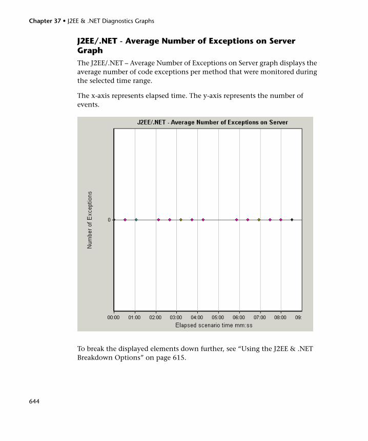
Chapter 37 • J2EE & .NET Diagnostics Graphs
644
J2EE/.NET - Average Number of Exceptions on Server GraphThe J2EE/.NET – Average Number of Exceptions on Server graph displays the average number of code exceptions per method that were monitored during the selected time range.
The x-axis represents elapsed time. The y-axis represents the number of events.
To break the displayed elements down further, see “Using the J2EE & .NET Breakdown Options” on page 615.
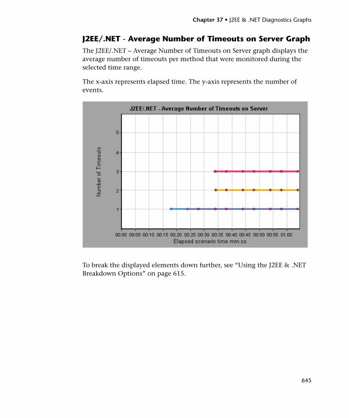
Chapter 37 • J2EE & .NET Diagnostics Graphs
645
J2EE/.NET - Average Number of Timeouts on Server GraphThe J2EE/.NET – Average Number of Timeouts on Server graph displays the average number of timeouts per method that were monitored during the selected time range.
The x-axis represents elapsed time. The y-axis represents the number of events.
To break the displayed elements down further, see “Using the J2EE & .NET Breakdown Options” on page 615.

Chapter 37 • J2EE & .NET Diagnostics Graphs
646
Part V
Appendixes

648
649
A Interpreting Analysis Graphs
LoadRunner Analysis graphs present important information about the performance of your load test scenario. Using these graphs, you can identify and pinpoint bottlenecks in your application and determine what changes are needed to improve its performance.
This appendix includes:
➤ Analyzing Transaction Performance on page 650
➤ Using the Web Page Diagnostics Graphs on page 652
➤ Using Auto Correlation on page 654
➤ Identifying Server Problems on page 659
➤ Identifying Network Problems on page 660
➤ Comparing Scenario Results on page 661
Note: The appendix presents examples from Web load tests.
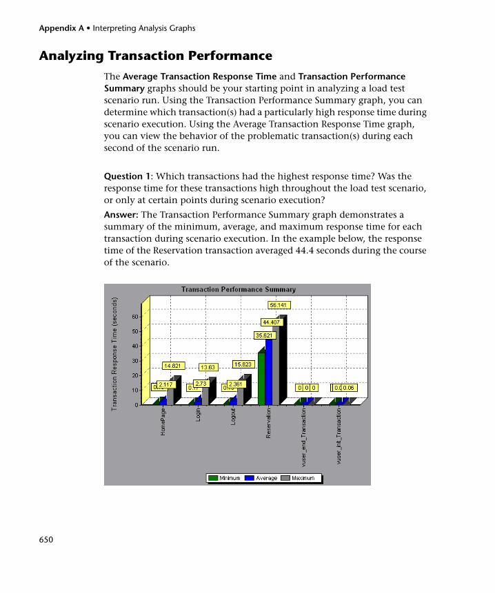
Appendix A • Interpreting Analysis Graphs
650
Analyzing Transaction Performance
The Average Transaction Response Time and Transaction Performance Summary graphs should be your starting point in analyzing a load test scenario run. Using the Transaction Performance Summary graph, you can determine which transaction(s) had a particularly high response time during scenario execution. Using the Average Transaction Response Time graph, you can view the behavior of the problematic transaction(s) during each second of the scenario run.
Question 1: Which transactions had the highest response time? Was the response time for these transactions high throughout the load test scenario, or only at certain points during scenario execution?
Answer: The Transaction Performance Summary graph demonstrates a summary of the minimum, average, and maximum response time for each transaction during scenario execution. In the example below, the response time of the Reservation transaction averaged 44.4 seconds during the course of the scenario.
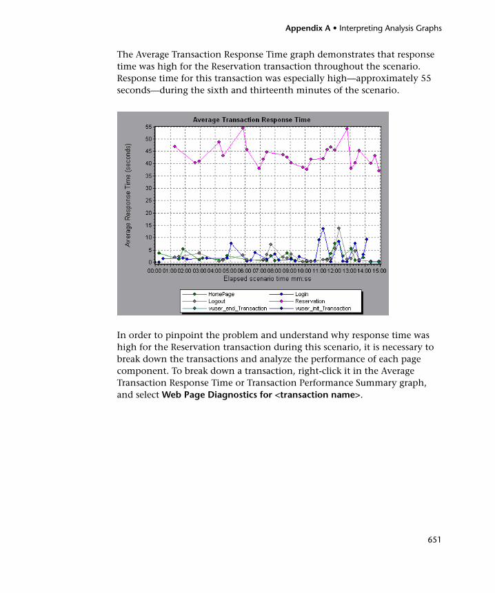
Appendix A • Interpreting Analysis Graphs
651
The Average Transaction Response Time graph demonstrates that response time was high for the Reservation transaction throughout the scenario. Response time for this transaction was especially high—approximately 55 seconds—during the sixth and thirteenth minutes of the scenario.
In order to pinpoint the problem and understand why response time was high for the Reservation transaction during this scenario, it is necessary to break down the transactions and analyze the performance of each page component. To break down a transaction, right-click it in the Average Transaction Response Time or Transaction Performance Summary graph, and select Web Page Diagnostics for <transaction name>.
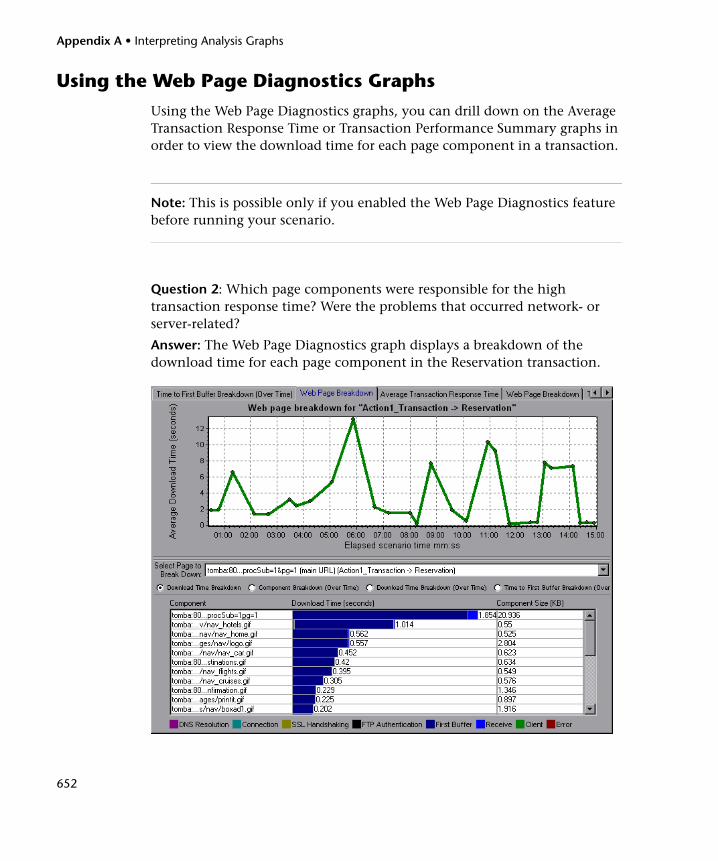
Appendix A • Interpreting Analysis Graphs
652
Using the Web Page Diagnostics Graphs
Using the Web Page Diagnostics graphs, you can drill down on the Average Transaction Response Time or Transaction Performance Summary graphs in order to view the download time for each page component in a transaction.
Note: This is possible only if you enabled the Web Page Diagnostics feature before running your scenario.
Question 2: Which page components were responsible for the high transaction response time? Were the problems that occurred network- or server-related?
Answer: The Web Page Diagnostics graph displays a breakdown of the download time for each page component in the Reservation transaction.
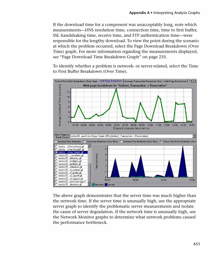
Appendix A • Interpreting Analysis Graphs
653
If the download time for a component was unacceptably long, note which measurements—DNS resolution time, connection time, time to first buffer, SSL handshaking time, receive time, and FTP authentication time—were responsible for the lengthy download. To view the point during the scenario at which the problem occurred, select the Page Download Breakdown (Over Time) graph. For more information regarding the measurements displayed, see “Page Download Time Breakdown Graph” on page 235.
To identify whether a problem is network- or server-related, select the Time to First Buffer Breakdown (Over Time).
The above graph demonstrates that the server time was much higher than the network time. If the server time is unusually high, use the appropriate server graph to identify the problematic server measurements and isolate the cause of server degradation. If the network time is unusually high, use the Network Monitor graphs to determine what network problems caused the performance bottleneck.
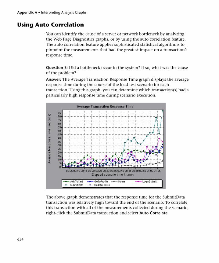
Appendix A • Interpreting Analysis Graphs
654
Using Auto Correlation
You can identify the cause of a server or network bottleneck by analyzing the Web Page Diagnostics graphs, or by using the auto correlation feature. The auto correlation feature applies sophisticated statistical algorithms to pinpoint the measurements that had the greatest impact on a transaction’s response time.
Question 3: Did a bottleneck occur in the system? If so, what was the cause of the problem?
Answer: The Average Transaction Response Time graph displays the average response time during the course of the load test scenario for each transaction. Using this graph, you can determine which transaction(s) had a particularly high response time during scenario execution.
The above graph demonstrates that the response time for the SubmitData transaction was relatively high toward the end of the scenario. To correlate this transaction with all of the measurements collected during the scenario, right-click the SubmitData transaction and select Auto Correlate.
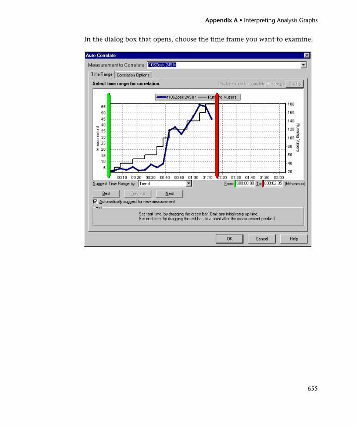
Appendix A • Interpreting Analysis Graphs
655
In the dialog box that opens, choose the time frame you want to examine.
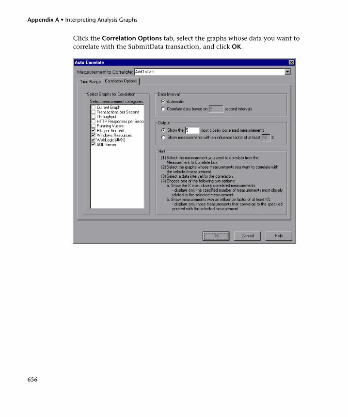
Appendix A • Interpreting Analysis Graphs
656
Click the Correlation Options tab, select the graphs whose data you want to correlate with the SubmitData transaction, and click OK.
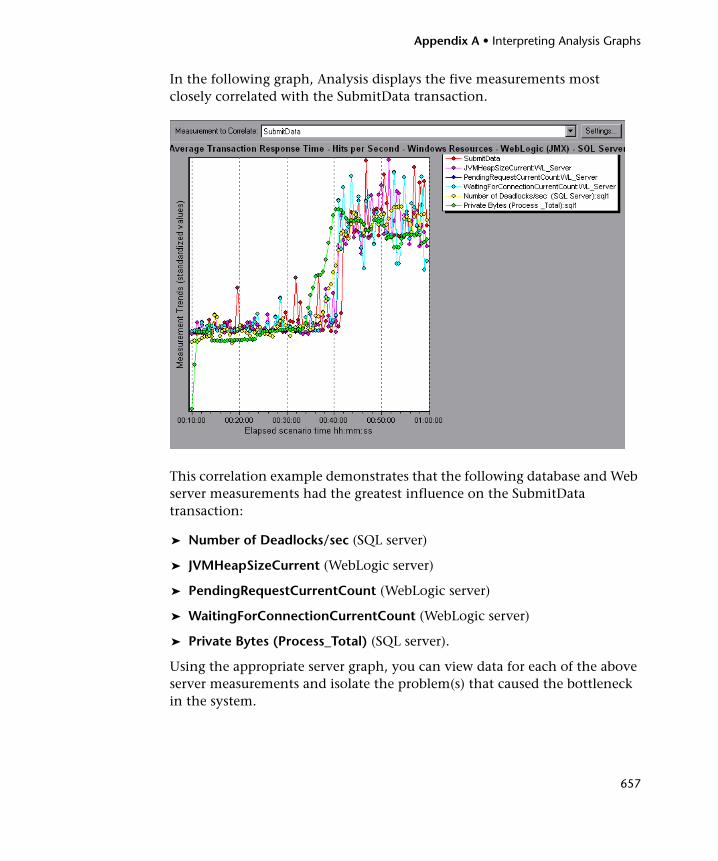
Appendix A • Interpreting Analysis Graphs
657
In the following graph, Analysis displays the five measurements most closely correlated with the SubmitData transaction.
This correlation example demonstrates that the following database and Web server measurements had the greatest influence on the SubmitData transaction:
➤ Number of Deadlocks/sec (SQL server)
➤ JVMHeapSizeCurrent (WebLogic server)
➤ PendingRequestCurrentCount (WebLogic server)
➤ WaitingForConnectionCurrentCount (WebLogic server)
➤ Private Bytes (Process_Total) (SQL server).
Using the appropriate server graph, you can view data for each of the above server measurements and isolate the problem(s) that caused the bottleneck in the system.
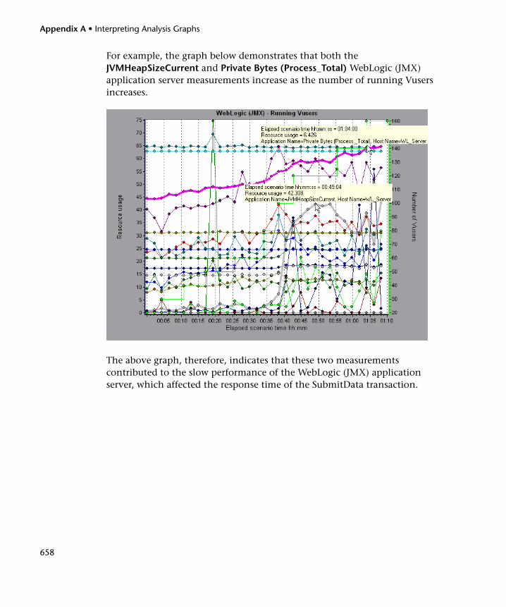
Appendix A • Interpreting Analysis Graphs
658
For example, the graph below demonstrates that both the JVMHeapSizeCurrent and Private Bytes (Process_Total) WebLogic (JMX) application server measurements increase as the number of running Vusers increases.
The above graph, therefore, indicates that these two measurements contributed to the slow performance of the WebLogic (JMX) application server, which affected the response time of the SubmitData transaction.
Appendix A • Interpreting Analysis Graphs
659
Identifying Server Problems
Web site performance problems can be a result of many factors. Nearly half of the performance problems, however, can be traced to Web, Web application, and database server malfunctioning. Dynamic Web sites that rely heavily on database operations are particularly at risk for performance problems.
The most common database problems are inefficient index design, fragmented databases, out-of-date statistics, and faulty application design. Database system performance can therefore be improved by using smaller result sets, automatically updating data, optimizing indexes, frequently compacting data, implementing a query or a lock on time-outs, using shorter transactions, and avoiding application deadlocks.
In twenty percent of load tests, Web and Web application servers are found to be the cause of performance bottlenecks. The bottlenecks are usually the result of poor server configuration and insufficient resources. For example, poorly written code and DLLs can use nearly all of a computer’s processor time (CPU) and create a bottleneck on the server. Likewise, physical memory constraints and mismanagement of server memory can easily cause a server bottleneck. It is therefore advisable to check both the CPU and physical memory of your server before exploring other possible causes of poor Web or Web application server performance.
For information about other useful Web, Web application, and database server measurements, refer to the HP LoadRunner Controller User Guide.
HTTPS Problems
Excessive use of HTTPS and other security measures can quickly exhaust server resources and contribute to system bottlenecks. For example, when HTTPS is implemented on the Web server during a load test, system resources are quickly exhausted by a relatively small load. This is caused by secured socket layer (SSL) resource-intensive operations.
Appendix A • Interpreting Analysis Graphs
660
Continuously open connections can also drain server resources. Unlike browsers, servers providing SSL services typically create numerous sessions with large numbers of clients. Caching the session identifiers from each transaction can quickly exhaust the server’s resources. In addition, the "keep-alive"enhancement features of most Web browsers keep connections open until they are explicitly terminated by the client or server. As a result, server resources may be wasted as large numbers of idle browsers remain connected to the server.
The performance of secured Web sites can be improved by:
➤ Fine-tuning the SSL and HTTPS services according to the type of application
➤ Using SSL hardware accelerators, such as SSL accelerator appliances and cards
➤ Changing the level of security according to the level of sensitivity of the data (i.e., changing the key length used for public-key encryption from 1,024 to 512 bits)
➤ Avoiding the excessive use of SSL and redesigning those pages that have low levels of data sensitivity to use regular HTTPS
Identifying Network Problems
Network bottlenecks can usually be identified when the load increment is considerable and is not significantly affecting any of the server side components, as in the case of informational sites using many static Web pages. In twenty-five percent of such cases, the pipe to the Internet cannot sufficiently handle the desired load and causes delays in incoming and outgoing requests. In addition, bottlenecks are frequently uncovered between the Web site and the ISP.
Using the Network Monitor graphs, you can determine whether, in fact, the network is causing a bottleneck. If the problem is network-related, you can locate the problematic segment so that it can be fixed.
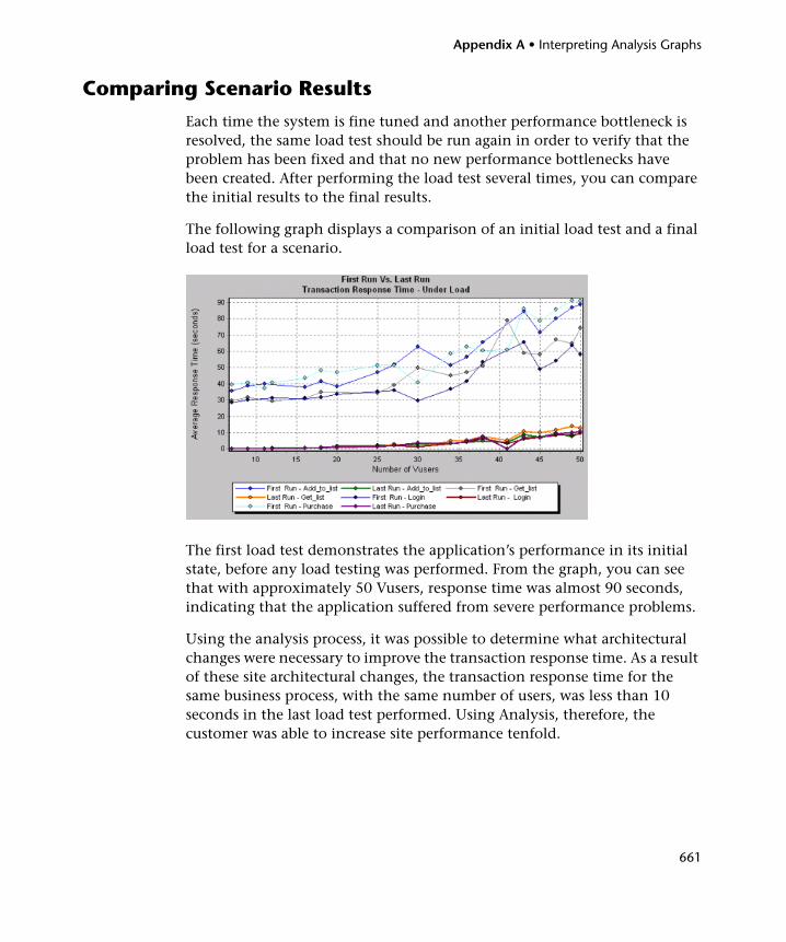
Appendix A • Interpreting Analysis Graphs
661
Comparing Scenario Results
Each time the system is fine tuned and another performance bottleneck is resolved, the same load test should be run again in order to verify that the problem has been fixed and that no new performance bottlenecks have been created. After performing the load test several times, you can compare the initial results to the final results.
The following graph displays a comparison of an initial load test and a final load test for a scenario.
The first load test demonstrates the application’s performance in its initial state, before any load testing was performed. From the graph, you can see that with approximately 50 Vusers, response time was almost 90 seconds, indicating that the application suffered from severe performance problems.
Using the analysis process, it was possible to determine what architectural changes were necessary to improve the transaction response time. As a result of these site architectural changes, the transaction response time for the same business process, with the same number of users, was less than 10 seconds in the last load test performed. Using Analysis, therefore, the customer was able to increase site performance tenfold.

Appendix A • Interpreting Analysis Graphs
662
663
A
Activity reports 500Adobe Reader 16advanced display settings 66
chart 67series 67
Analysisinterpreting graphs 649overview 23sessions 25
Analysis API 40analysis graph data
determining coordinates of a point 102
Analyzing a Performance Center Load Test 157
Antara FlameThrower graph 261Apache Server graph 287Application Component graphs 421Application Deployment Solutions graphs
455Ariba graph 301ASP graph 328ATG Dynamo graph 304auto correlating measurements
about 108example 654
Average Transaction Response Time graph 198
Average Transaction Response Time graph, auto correlation 654
B
breaking downJ2EE/.NET diagnostics data 609Oracle 11i transactions 570Siebel DB transactions 556Siebel diagnostics data 528transactions 228
BroadVision graph 308
C
chart settings 67Check Point FireWall-1 graph 282Citrix MetaFrame XP
Application Deployment Solutions graph 456
Client TimePage Download Time Breakdown
graph 237closing Analysis automatically 78ColdFusion graph 316collating execution results 26COM+
Average Response Time graph 429Breakdown graph 427Call Count Distribution graph 433Call Count graph 431Call Count Per Second graph 435COM+ graph 423Total Operation Time Distribution
graph 439Total Operation Time graph 437
compacting a database 54comparing scenario results 661Component Hierarchical Path dialog box
100
Index
Index
664
Configure Performance Center Connection dialog box 160
configuring dataaggregation 42options 41
configuring measurement options 71connecting
to Performance Center 159to Quality Center 150
Connection time in Page Download Time Breakdown graph 236
Connections graph 221Connections per Second graph 222Controller output messages 121Cross Result
generating 130graphs 127
CSV fileexporting to 70
Customizing the Layout of Analysis Windows 36
D
Data Import 173Data Point report 504Data Points (Average) graph 250Data Points (Sum) graph 248Data Time Range 44database
compacting 54options 50
Date Format 49DB2 graph 362Detailed Transactions reports 506Details button 125disconnecting
from Performance Center 161from Quality Center 153
display options, basic 63DNS Resolution time in Page Download
Time Breakdown graph 236documentation, online 16Downloaded Component Size graph 245drilling down specific graph measurements
102
E
Editing MainChart dialog boxAdding Comments and Arrows 74Chart tab 67Series tab 67
enlarging graphs 61ERP/CRM Server Resource graphs 399Error graphs 191Error Statistics
(by Description) graph 193graph 192
Error Time in Page Download Time Breakdown graph 237
Errors per Second(by Description) graph 196graph 195
Excel fileexporting to 115viewing 499
export datagraph data 115raw data 117
F
Failed Transaction report 503Failed Vuser report 504filter conditions, setting in Analysis 81filtering graphs 79First Buffer time in Page Download Time
Breakdown graph 236FTP Authentication time in Page Download
Time Breakdown graph 237Fujitsu INTERSTAGE graph 318
G
granularity 105Graph Data window 115Graph Settings dialog box 81graph types, Analysis
Application Component 421Application Deployment Solutions
455Database Server Resources 361
Index
665
ERP/CRM Server Resource Monitor 399
Errors 191FireWall Server Monitor 281J2EE/.NET Diagnostics 605Java Performance 417Middleware Performance 465Network Monitor 275Network monitor 275Oracle 11i Diagnostics 563SAP Diagnostics 577Siebel DB Diagnostics 547Siebel Diagnostics 523Streaming Media Resources 389System Resources 251Transaction 197User-Defined Data Points 247Vuser 187Web Application Server Resources 299Web Page Diagnostics 225Web Resources 209Web Server Resources 285
graphs 27Antara FlameThrower 261Apache 287Ariba 301ATG Dynamo 304Average Transaction Response Time
198BroadVision 308Check Point FireWall-1 282Citrix MetaFrame XP 456ColdFusion 316COM+ 423COM+ Average Response Time 429COM+ Breakdown 427COM+ Call Count 431COM+ Call Count Distribution 433COM+ Call Count Per Second 435COM+ Total Operation Time 437COM+ Total Operation Time
Distribution 439Connections 221Connections per Second 222Data Points (Average) 250Data Points (Sum) 248
DB2 362Downloaded Component Size 245Error Statistics 192Error Statistics (by Description) 193Errors per Second 194, 195Errors per Second (by Description)
196Fujitsu INTERSTAGE 318Hits per Second 211HTTP Responses per Second 214HTTP Status Code Summary 213IBM WebSphere MQ 469Infrastructure Resources 473iPlanet (NAS) 319iPlanet (SNMP) 293iPlanet/Netscape 291J2EE 418J2EE Average Method Response Time
629, 639J2EE Average Number of Exceptions
634, 644J2EE Average Number of Timeouts
635, 645J2EE Method Calls per Second 633,
643J2EE Time Spent in Element 630, 640J2EE Transaction Response Time
Server Side 628, 638J2EE Transactions per Second 632,
642Microsoft Active Server Pages (ASP)
328Microsoft IIS 289.NET Average Response Time 443.NET Breakdown 441.NET Call Count 444.NET Call Count Distribution 446.NET Call Count per Second 447.NET Resources 450.NET Total Operation Time 449.NET Total Operation Time
Distribution 448Network Client 474Network Delay Time 277Network Segment Delay 279Network Sub-Path Time 278
Index
666
Oracle 377Oracle 11i Side Transactions by SQL
Stage 575Oracle 11i SQL Average Execution
Time 576Oracle 11i Transactions 573Oracle9iAS HTTP 329Page Component Breakdown 231Page Component Breakdown (Over
Time) 233Page Download Time Breakdown 235Page Download Time Breakdown
(Over Time) 239Pages Downloaded per Second 217PeopleSoft (Tuxedo) 414RealPlayer Client 391RealPlayer Server 393Rendezvous 190Retries per Second 219Retries Summary 220Running Vusers 188SAP 400SAP Application Processing Time
Breakdown 598SAP Average Dialog Step Response
Time Breakdown 594SAP Average Transaction Response
Time 592SAP Database Time Breakdown 597SAP Dialog Steps per Second 601SAP Interface Time Breakdown 600SAP OS Monitor 603SAP Portal 406SAP secondary graphs 600SAP Server Time Breakdown 596SAP Server Time Breakdown (Dialog
Steps) 595SAP System Time Breakdown 599SAP Work Processes 602SAPGUI 403Server Resources 258Siebel Area Average Response Time
543Siebel Area Call Count 544Siebel Area Total Response Time 545Siebel DB Side Transactions by SQL
Stage 560Siebel DB Transactions 558Siebel Request Average Response Time
546Siebel Server Manager 409Siebel SQL Average Execution Time
561Siebel Transaction Average Response
Time 542Siebel Web Server 412SilverStream 334SiteScope 273SNMP Resources 260SQL Server 380SSLs per Second 223Sybase 382Throughput 212Time to First Buffer Breakdown 241Time to First Buffer Breakdown (Over
Time) 243Total Transactions per second 202Transaction Performance Summary
204Transaction Response Time
(Distribution) 208Transaction Response Time
(Percentile) 206Transaction Response Time (Under
Load) 205Transaction Summary 203Transactions per second 201Tuxedo Resources 466UNIX Resources 256Vuser Summary 189WebLogic (JMX) 339WebLogic (SNMP) 336WebSphere 342WebSphere (EPM) 353WebSphere Application Server 349Windows Media Player Client 396Windows Media Server 394Windows Resources 252
graphs, working withaccessing 30background image 67crossing results 127
Index
667
display options 62merging 131opening 30pre-filtering 30superimposing 132
H
Hierarchical Path dialog box 100Hits per Second graph 211HP Diagnostics, enabling 606HP Software Support Web site 18HP Software Web site 19HTML, creating reports 499HTTP Responses per Second graph 214HTTP Status Code Summary graph 213HTTPS 659
I
IBM WebSphere MQ graph 469IIS graph 289Importing Data 173Infrastructure Resources
graphs 473monitoring 473
interpreting Analysis graphs 649iPlanet
(NAS) graph 319(SNMP) graph 293
iPlanet/Netscape graph 291
J
J2EEAverage Method Response Time graph
629, 639Average Number of Exceptions graph
634, 644Average Number of Timeouts graph
635, 645Method Calls per Second graph 633,
643Time Spent in Element graph 630,
640Transaction Response Time Server
Side graph 628, 638
Transactions per Second graph 632, 642
J2EE/.NET Diagnostics graphs 605call stack 619chain of calls 619class level 612enabling 606example 609layer level 611Measurements Tree window 619method/query level 613SQL logical name 627, 637summary report 607transaction level 610viewing 609
Java Performance graphs 417
K
Knowledge Base 18
L
legend preferences 67Legend window 68load test, analyzing 157LoadRunner Analysis User’s Guide 17LoadRunner Controller User’s Guide 17LoadRunner Installation Guide 18LoadRunner Monitor Reference 17lr_user_data_point 248
M
Measurement Description dialog box 70measurement trends, viewing 107measurements
auto-correlating 108measurment options
configuring 71Media Player Client graph 396merging graphs 131Microsoft
Active Server Pages (ASP) graph 328IIS graph 289Word Reports 509
Middleware Performance graphs 465
Index
668
N
.NETAverage Response Time graph 443Breakdown graph 441Call Count Distribution graph 446Call Count graph 444Call Count per Second graph 447Resources graph 450Total Operation Time Distribution
graph 448Total Operation Time graph 449
NetworkDelay Time graph 277Segment Delay graph 279Sub-Path Time graph 278
Network Client graph 474Network Monitor graphs 275
O
online documentation 16Open a New Graph dialog box 32Options dialog box
Database tab 50General tab 48Result Collection tab 42Web Page Breakdown tab 57
Oracle 11iDiagnostics graphs 563Side Transactions by SQL Stage graph
575Side Transactions graph 573SQL Average Execution Time graph
576Oracle graph 377Oracle9iAS HTTP graph 329output messages, viewing 121Output window
drilling down on log information 124filtering messages 125saving messages to a file 125sorting messages 126viewing message detail 125
overlay graphs 132
P
packets 276Page
Component Breakdown (Over Time) graph 233
Component Breakdown graph 231Download Time Breakdown (Over
Time) graph 239Download Time Breakdown graph
235Pages Downloaded per Second graph 217PeopleSoft (Tuxedo) graph 414Performance Center
connecting to 159disconnecting from 161downloading session and result files
162uploading reports 165uploading session files 165
Performance reports 500pre-filtering graphs 30Printing Graphs or Reports 34printing graphs or reports 34
Q
Quality Centerconnecting to 150disconnecting from 153integration 149opening an existing session 154saving sessions to a project 156
R
raw data 114RealPlayer
Client graph 391Server graph 393
Receive timein Page Download Time Breakdown
graph 236Remote Function Call (SAP)
offline diagnostics (Analysis) 623Rendezvous graph 190reports 479
Index
669
accessing 30Data Point 504Detailed Transaction 506Failed Transaction 503Failed Vuser 504opening 30Scenario Execution 503SLA report 489Transaction Performance by Vuser
507reports, working with
activity and performance reports 500creating HTML 499displaying 501summary report 481transaction analysis 496viewer 501viewing summary 481
Retries per Second graph 219Retries Summary graph 220Running Vusers graph 188Run-Time settings
session 119viewing in Analysis 119
S
SAP Diagnosticsgraphs 577guided flow 580main view 580opening 579viewing 579
SAP graph 400SAP graphs
Application Processing Time Breakdown 598
Database Time Breakdown 597Interface Time Breakdown 600SAP Average Dialog Step Response
Time Breakdown 594SAP Average Transaction Response
Time 592SAP Secondary View
Dialog Steps per Second 601OS Monitor 603
Work Processes 602SAP Server Time Breakdown 596SAP Server Time Breakdown (Dialog
Steps) 595secondary graphs 600System Time Breakdown 599
SAP Portal graph 406SAPGUI graph 403Save as Template dialog box 76, 77saving Analysis session automatically 78scale factor
Streaming Media graphs 389Web Server Resource graphs 286
scale of graph 105Scenario Execution report 503scenario output messages, viewing 121Scenario Run-Time Settings dialog box 119scenario, comparing 661security problems 659Select Report Filename and Path dialog box
499Server Resources graph 258service level agreements, defining 135Session Information dialog box 59Session Step Run-Time Settings dialog box
119sessions, creating in Analysis 25Set Dimension Information dialog box 98Siebel
Area Average Response Time graph 543
Area Call Count graph 544Area Total Response Time graph 545
Siebel DB Diagnosticsgraphs 547synchronizing clock settings 551viewing 553
Siebel DB Side Transactions by SQL Stage graph 560
Siebel DB Side Transactions graph 558Siebel Diagnostics
area level 529call stack 534chain of calls 534example 528graphs 523

Index
670
layer level 529Measurements Tree window 535script level 530server level 531sub-area level 530transaction level 528viewing 528
Siebel Request Average Response Time graph 546
Siebel Server Manager graph 409Siebel SQL Average Execution Time graph
561Siebel Transaction Average Response Time
graph 542Siebel Web Server graph 412SilverStream graph 334SiteScope graph 273SLA
defining 135report 489summary report 484
SNMP Resources graph 260spreadsheet view 114SQL Server graph 380SSL Handshaking time in Page Download
Time Breakdown graph 236SSLs per Second graph 223standardizing y-axis values 107Streaming Media graphs 389summary data, viewing 26Summary report 481
J2EE/.NET Diagnostics graphs 607no SLA 481SAP Diagnostics 583Siebel 526with SLA 484
summary report 481superimposing graphs 132Sybase graph 382synchronizing Siebel clock settings 551
T
templatesapplying 76saving 77
three-dimensionalchart display 65selecting 67
Throughput graph 212Time to First Buffer Breakdown
graph 241Over Time graph 243
Total Errors per Secondgraph 194
Total Transactions per Second graph 202transaction analysis 491
dialog box 493report 496settings 495
Transaction graphs 197Transaction Response Time graphs
Average 198Distribution 208Percentile 206Under Load 205
transactionsbreakdown 228breaking down Oracle 11i 570breaking down Siebel DB 556Transaction Performance by Vuser
report 507Transaction Performance Summary
graph 204Transactions per Second graph 201
Troubleshooting and Knowledge Base 18Tuxedo, Middleware Performance graph 466
U
UNIX Resources graph 256uploading session files and reports 165user_data_point function 248User-Defined Data Point graphs 247
Index
671
V
viewingmeasurement trends 107SAP Diagnostics summary 583Siebel summary report 526
VusersScenario Elapsed Time dialog box 99Vuser ID dialog box 98Vuser Summary graph 189
W
WAN Emulation 40Web Application Server Resource graphs 299Web Page Diagnostics Content Icons 229Web Page Diagnostics graphs 225
activating 228using 652
Web Resource graphs 209Web Server Resource graphs 285WebLogic
(JMX) graph 339(SNMP) graph 336
WebSphere(EPM) graph 353Application Server graph 349graph 342
Windows Media Server graph 394Windows Resources graph 252Word Reports 509
X
x-axis interval 105
Y
y-axis values, standardizing 107
Z
zoom in on a graph 61

Index
672