how useful are formal hierarchies? a case study on ... · sabyasachi chatterjee amit acharyay...
TRANSCRIPT
How useful are formal hierarchies? A case study on averaging
dislocation dynamics to define meso-macro plasticity
Sabyasachi Chatterjee∗ Amit Acharya†
Abstract
A formal hierarchy of exact evolution equations are derived for physically relevant space-timeaverages of state functions of microscopic dislocation dynamics. While such hierarchies areundoubtedly of some value, a primary goal here is to expose the intractable complexity of suchsystems of nonlinear partial differential equations that, furthermore, remain ‘non-closed,’ andtherefore subject to phenomenological assumptions to be useful. It is instead suggested that suchhierarchies be terminated at the earliest stage possible and effort be expended to derive closurerelations for the ‘non-closed’ terms that arise from the formal averaging by taking into accountthe full-stress-coupled microscopic dislocation dynamics (as done in [CPZ+20]), a matter onwhich these formal hierarchies, whether of kinetic theory type or as pursued here, are silent.
1 Introduction
This paper is concerned with the formal derivation of governing field equations of increasinglydetailed space-time averaged behavior of microscopic dislocation dynamics, and assessing the valueof such systems. The microscopic dislocation dynamics is posed as a system of pde, capable ofrepresenting the dynamics of a collection of possibly tangled smooth curves representing dislocationcore cylinders, each core cylinder movable by a combination of glide and climb due to the action ofa vectorial velocity field. The velocity field is determined, following well-accepted notions, purelyfrom the dislocation density field (with the possibly tangled web of core cylinders viewed simplyas appropriate smooth localizations in space of the dislocation density field), and the (nonlinearcrystal elastic) stress field in the body; even when linear elasticity is used, the point-wise Burgersvector direction and line direction (information built into the dislocation density field) are adequateto describe the motion of edge segments, and the motion of screws are restricted to within ageometrically defined set of planes. In any case a resolution into slip system dislocation densitiesis not essential (cf. [ZCA13]). This pde system is adequate for representing the plasticity of theconstituent material when atomic length scales are resolved - we refer to this system as FieldDislocation Mechanics (FDM). We are interested in obtaining the implications of this model whenthe resolved length (and time) scales are much coarser, i.e. we are interested in obtaining someinformation on the nature of the governing evolution equations for increasingly detailed descriptionsof averaged behavior of this microscopic system, appropriate for coarser-length and time scales.We emphasize that the derived averaged equations represent exact, but non-closed, statementsof evolution of the defined average variables, without any compromise on the inherent kinematic
∗Dept. of Civil & Environmental Engineering, Carnegie Mellon University, Pittsburgh, PA [email protected].†Dept. of Civil & Environmental Engineering, and Center for Nonlinear Analysis, Carnegie Mellon University,
Pittsburgh, PA 15213. [email protected].
1

constraints of the microscopic system (e.g. the connectedness of the dislocation lines representedby the solenoidal property of the microscopic dislocation density field).
The above line of inquiry was initiated in [AR06, AC12]; as will be shown in this paper, the exactequations of evolution become exceedingly complex and cumbersome and it was suggested in [AR06]that closure assumptions be made at a relatively lower level to maintain tractability (while allowingfor the inclusion of all that is known in the physics-based phenomenological modeling of plasticdeformation and strength, e.g. [KAA75]) and refining the description as required for greater fidelity.We will refer to this approach as the MFDM (Mesoscale Field Dislocation Mechanics) approach toplasticity.
In the Continuum Dislocation Dynamics (CDD) framework of Hochrainer and collaborators [HZG07,Hoc16, MZ18], models are developed based on a kinetic theory-like framework, starting from theassumption that a fundamental statement for the evolution of a number density function on thespace of dislocation segment positions and orientations is available at the microscopic level. Thismicroscopic governing equation is non-closed even if one knows completely the rules of physicalevolution of individual dislocations segments of connected lines; one would need to study the be-havior of an ensemble of dislocation dynamics evolutions to define, and then also only in principle,the evolution of such a number density function (cf. [HZG07, Sec 3.1, 5]) - this detail is builtinto the state-space velocity function introduced in [HZG07], which cannot be simply defined bya well-accepted statement like the Peach-Kohler force for a segment of a real-space description ofa dislocation line. Furthermore, Equations (7) and (11) of [HZG07], the fundamental statementof evolution governing the number density function (a ‘collective’ quantity), are postulated with-out fundamental justification. This is in contrast to FDM where the fundamental justification forthe statement of microscopic dynamics is the integral statement of conservation of Burgers vector,a physically observed fact (which does not imply a conservation of the ‘number’ of dislocations,whether loops or otherwise, as stated in [HZG07, Sec. 4], and as demonstrated in exercises relatedto annihilation and nucleation [GAM15]); then, the equations of MFDM follow strictly from FDMon averaging, without any further assumptions. Returning to CDD, on making various assumptionsfor tractability, the theory produces (non-closed) statements of evolution for the averaged disloca-tion density (akin to the mesoscale Nye tensor field), the total dislocation density (similar to anappropriate sum of the averaged Nye tensor density) and, these densities being defined as physicalscalars, and an associated curvature density field. Closure assumptions are made to cut off infinitehierarchies, which is standard for averaging based on nonlinear ‘microscopic equations’, and fur-ther closure assumptions for constitutive statements are made based on standard thermodynamicarguments [Hoc16].
The model in [XEA15] belongs to the same mathematical class as MFDM but with more compli-cated constitutive structure related to multiple-slip behavior [DAS16]. It assumes geometricallylinear kinematics for the total deformation coupled to a system of stress-dependent, nonlineartransport equations for vector-valued slip-system dislocation densities. These slip system den-sity transport equations involve complicated, phenomenological constitutive assumptions relatedto cross-slip, and the authors of [XEA15] promote the point of view that dislocation patterningis related to the modeling of slip system dislocation densities and cross-slip. An attempt to un-derstand emergence of microstructure in 1-d setting was made in [DAS16], and in 3-d and finitedeformation setting was made in [AA20a]. They concluded that in all likelihood, such complexityis not essential for the emergence of dislocation microstructure in this family of models.
Despite postulating the microscopic dynamics on which their entire approach is based, makingphenomenological closure assumptions of their own, and making ad-hoc choices of cutting off the
2

infinite hierarchy of their equations, the CDD authors have criticized the MFDM approach asinadequate for describing the plasticity of metals [HZG07, Hoc16, MZ18]. The authors of [XEA15]have criticized MFDM for using a phenomenological approach and for the lack of resolution into slipsystems in order to model cross slip. One goal of this paper is to show that the criticisms leveledagainst the MFDM approach in [SHZG11, XEA15, MZ18] are unfounded, at least in comparisonto the standards of these works.
The MFDM approach starts from a well-accepted fundamental microscopic dynamical statement(unlike CDD), and produces an exact hierarchy of equations for any desired level of detail inthe coarse description as an implication of this fundamental microscopic dynamics. Extending thework in [AC12], this paper explicitly shows that while the MFDM approach can easily accommodatedescriptors like slip system dislocation densities and define precise hierarchies of evolution equationsfor them, such an enterprise comes at a significant cost in complexity and tractability of theresulting model, and shows the exact nature of phenomenology and gross approximation thatwould necessarily be inherent in any proposed formalism for coarse-grained dislocation dynamics(e.g., [SHZG11, XEA15]) that does not consider head-on the question of averaging the stress-coupledinteraction-related dynamics of dislocations.
This paper is organized as follows. In Section 2, we apply the averaging procedure utilized in [Bab97]to generate an infinite hierarchy of nonlinear coarse equations corresponding to a fine dynamics,which (essentially) cannot be solved. In Section 3, we apply the averaging procedure to derive thecoarse evolution of averaged total dislocation density and demonstrate, using a simple example,that the averaged dislocation density of an expanding circular loop increases. In Section 3.2, wepresent a refined description of the variables with respect to individual slip systems, reflectiveof a crystal plasticity description and present the coarse evolution of these variables, namely theaveraged dislocation density tensor and the averaged total dislocation density. In order to do so,we define a characteristic function, which indicates whether any given position has a dislocation ofa particular slip system. We show how the coarse evolution of these variables are very cumbersomeand hence, why it is reasonable to close the infinite hierarchy of non-closed system of equations ata low level. It is also important to generate lower level closure assumptions that account for thestress coupled dynamics of dislocations. Such work has been demonstrated in [CPZ+20].
2 Hierarchy of averaged equations for nonlinear microscopic equa-tions: the basic idea
In this section, we will utilize an averaging procedure used in the literature for multiphase flows(see [Bab97]). For a microscopic field f given as a function of space and time, the mesoscopicspace-time-averaged field f [AR06, AC12] is given as
f(x, t) =1∫
I(t)
∫Ω(x)w(x− x′, t− t′)dx′dt′
∫=
∫Bw(x− x′, t− t′)f(x′, t′)dx′dt′, (1)
where B is the body and I a sufficiently large interval of time. In the above, Ω(x) is a boundedregion within the body around the point x with linear dimension of the order of the spatial resolutionof the macroscopic model we seek, and I(t) is a bounded interval in I containing t. The weightingfunction w is non-dimensional, assumed to be smooth in the variables x, x′, t, t′ and, for fixedx and t, have support (i.e. to be non-zero) only in Ω(x) × I(t) when viewed as a function of(x′, t′).
3

The one-dimensional analogue of (1) is
∂t′f = F (f, ∂x′f), (2)
where x′ is the spatial coordinate and t′ is time and f is a function of x′ and t′. We call the systemgiven by equation (2) as the fine scale system.
We aim to understand the macroscopic evolution of the fine dynamics (2) in terms of averaged(coarse) variables. To do so, the averaging operator (1) is applied to both sides of (2), whichresults in the following:
∂
∂tf(x, t) = F (f, ∂x′f)(x, t). (3)
We denote A0 := f and A01 := ∂tA0 = F . The fluctuation of function f is defined as:
Σf (x′, t′, x, t) := f(x′, t′)− f(x, t). (4)
The average of the product (p) of two variables f and g is given by
f(p)g =f + (f − f)(p)g + (g − g)
=f(p)g + f(p)(g − g) + (f − f)(p)g + (f − f)(p)(g − g)
=f(p)g + f(p)Σg + g(p)Σf + Σf (p)Σg
=f(p)g + Σf (p)Σg, (5)
so that
f(p)g − f(p)g = f(p)g − f(p)g = Σf (p)Σg.
Here, f and g can be scalar, vector or tensor valued. Some examples of the product (p) are scalarmultiplication, vector inner product, tensor inner product, cross product of a tensor with a vectoretc. For example, if f and g are scalar and (p) is the scalar multiplication operator,
fg = f g + ΣfΣg. (6)
Using (5), we obtain the average of product of three variables as
f(p)g(p)h =f(p)g(p)h+ Σf (p)Σg(p)h = f(p)g(p)h+ Σg(p)Σh+ Σf (p)Σg(p)h
=f(p)g(p)h+ f(p)Σg(p)Σh + Σf (p)Σg(p)h. (7)
Similarly, for f , g and h scalars and (p) the scalar multiplication operator,
fgh = f g h+ f Σg Σh + Σf Σg h. (8)
Equations (6), (7) and (8) show that the averages of products of two or more variables are not theproducts of their averages.
4

It can be shown using (2), (3) and (4) that
∂ttA0 = ∂tA01 = ∂2F∂1F∂xA0 + ∂2F∂2F∂xxA0 +A011 + Σ(∂2F∂1F )Σ(∂x′f) + Σ(∂2F∂2F )Σ(∂x′x′f),(9)
where A011 := ∂1FF .
Thus, in the coarse evolution of F , new terms (e.g. ∂2F∂1F ) emerge and therefore, it is necessaryto augment (9) with coarse evolution equations of the new terms (that appear on the rhs of (9)),namely the following:
∂t(∂2F∂1F
)= G1
∂t(∂2F∂2F
)= G2
∂t
(Σ(∂2F∂1F )Σ(∂x′f)
)= G3
∂t
(Σ(∂2F∂2F )Σ(∂x′x′f)
)= G4, (10)
where Gi (i = 1 to 4) are functionals of the state. In general, these functionals cannot be expressedas functionals of the independent fields of the averaged model, such relations being referred to as‘closure’ relations.
The functionals Gi can be generated by applying the averaging operator (1) to the fine scaleequations and decomposing the average of product of functions in the fine scale into product oftheir averages and their associated fluctuation terms. For example, the coarse evolution of ∂2F∂1F(which is given by G1 above) is
∂t(∂2F∂1F
)= ∂′t (∂2F∂1F ) = ∂′t (∂2F ) ∂1F + ∂2F∂′t (∂1F )
= H(∂1F ) + (∂2F )M = H∂1F +M∂2F + ΣHΣ∂1F + ΣMΣ∂2F ,
where H = ∂′t (∂2F ) and M = ∂′t (∂1F ). Thus, new terms appear in the coarse evolution of theterm ∂2F∂1F , and similarly for the other terms in (10). In this manner, we can generate an infinitehierarchy of nonlinear coarse equations corresponding to the fine dynamics (2). Solution of suchan infinite system is not possible.
It is therefore necessary to close the equations at a desired level, which means to use physics basedassumptions for the necessary terms instead of solving their exact evolution equation (for example,in equation (10) above, we might use closure assumptions for the functionals Gi on the rhs).Morever, even if the system was finite but large and could be solved (in principle), approximatingsolutions to nonlinear systems of pde is by no means a trivial task, so that it is definitely better toshift the focus from generating large formal hierarchies of nonlinear pde to generating controlled,with respect to accuracy, closure assumptions to maintain tractability.
3 Models of MFDM with varying coarse descriptors
The model of FDM [Ach01, Ach03, Ach04] represents the dynamics of a collection of dislocationlines at the atomic length scale. The field equations of FDM are as follows:
α = −curl(α× V )
curlχ = α
5

divχ = 0
div(gradz) = div(α× V +Lp)
div(C : gradu− z + χ) = 0. (11)
The tensor α is the dislocation density tensor, V is the dislocation velocity vector, C is the fourth-order, possibly anisotropic, tensor of linear elastic moduli, u is the total displacement vector, χ isthe incompatible part of the elastic distortion tensor, and u− z is a vector field whose gradient isthe compatible part of the elastic distortion tensor. Upon application of the averaging operator (1)defined in Section 2 to both sides of (11), we have the following system of averaged equations
α = −curl(α× V +Lp)
curlχ = α
divχ = 0
div(gradz) = div(α× V +Lp)
div(C : grad(u− z) + χ) = 0 (12)
[AR06]. The system (12) is called Mesoscale Field Dislocation Mechanics. Here, Lp is definedas
Lp := α× V −α× V , (13)
and it represents the strain rate produced by ‘statistically stored dislocations’. It follows from(5) that Lp is the average of the cross product of the fluctuation of α and V ( which meansLp = Σα × ΣV ). Consider a uniformly expanding square loop. Since α = b ⊗ l, where b is theBurgers vector density per unit area and l is the line direction at each point of the loop and bremains uniform along the loop, and both l and V change sign going from one side of the squareloop to the opposite side, both α = 0 and V = 0. However, α × V is identical for opposite sidesof the loop and does not cancel out and hence, Lp 6= 0.
3.1 Isotropic MFDM
We consider as descriptors of the system the averaged total dislocation density ρ and the plasticdistortion rate Lp, which are commonly used in the literature (also see [AC12]).
3.1.1 Evolution equation for averaged total dislocation density, ρl.
The total dislocation density is defined as
ρ := α : α. (14)
Suppose we have many dislocation segments in a box of volume V . We see that∫V ρdv
V =∑
iαi:αi liAi
V ,where αi, li and Ai (which is assumed to be |bi|2 up to a constant) are the dislocation density tensor,
line length and cross section area of segment i respectively. We also have that αi = |bi|mi⊗tiAi
, wherebi, mi and ti are the Burgers vector, Burgers vector direction and the line direction of segment i.
Therefore,∑
iαi:αi liAi
V = 1V
∑i|bi|2A2
iliAi = 1
V
∑i|bi|2|bi|4 li|bi|
2= 1V
∑i li, which is the averaged dislo-
cation density in the box. Since ρ is the microscopic total dislocation density,∫V ρdv
V is ρ averagedover V , which gives the averaged dislocation density of the box. This acts as a verification that ρis indeed the total dislocation density.
6

The space-time averaged total dislocation density ρ is given by
ρ = α : α+ Σα : Σα. (15)
This follows from (5) and shows that the average of the total dislocation density contains averageterms as well as averages of fluctuations. We can interpret this using Fig. 1 in which we see thatthe averaging box has many loops which are inside the box and there are some loops which arenot entirely contained inside the box. Since the Burgers vector is uniform over a loop, the averagedislocation density (b⊗ l) due to the loops which are contained in the box is 0 since the average ofthe line direction l over the loop cancels out. The only contribution to the first term on the rhs of(15) is from the loops which are not entirely contained in the averaging box. If our averaging boxhas a very large length scale, then most loops will be contained inside the box and as such, α ≈ 0and the main contribution to the averaged total dislocation density will come from the average ofthe fluctuation term given by the second term on the rhs of (15). The evolution of such fluctuationterms, as discussed in Section 2, will be given by other pde, which will themselves be non-closed,as they will contain other fluctuation terms. This will generate an infinite hierarchy of non-closedcumbersome pde, as will be shown next.
Figure 1: Dislocation loops in averaging box
The evolution of ρ is given by
ρ =− grad ρ · V − 2 ρ divV + 2 α : (divα⊗ V ) + 2 α : α gradV − Σgradρ · ΣV
− 2ΣρΣdivV + 2 α : (Σdivα ⊗ ΣV ) + 2Σα : Σdivα⊗V + 2 α : Σα ΣgradV
+ 2 Σα : Σα gradV . (16)
The derivation of (16) is given in Appendix A.1. As the averaging length scale becomes large, theRHS of (16) is dominated by the averages of the fluctuation terms.
Example: Circular dislocation loop
The evolution equation for ρ (as derived in Appendix A.1 and given by (35)) is
ρ = −gradρ · V − 2ρ(divV ) + 2α : (divα⊗ V ) + 2α : α gradV
Application of the averaging operator (1) to the above results in the following:
ρ = −gradρ · V − 2ρ(divV ) + 2α : (divα⊗ V ) + 2α : α gradV . (17)
7

!"!
#$#%
#&
#'(
)*
(!, *)(! + "!, *)
Figure 2: Top view of a uniformly expanding loop of radius R and width ∆R.
We aim to understand the evolution of ρ for the case of a circular dislocation loop of inner radiusR, width ∆R (see Fig. 2) and thickness t. The area of cross section of the loop is A = ∆R. t,which is assumed to be b2, where b is the magnitude of the Burgers vector b. The radial unitvector is er = cosθex + sinθey, while the tangential unit vector is eθ = −sinθex + cosθey. Let usassume that its velocity has the same magnitude for all points (r, θ, z) of the loop (where z is thespatial coordinate along the thickness) and points radially outwards. Hence, the velocity is givenby V = v(r) er, where v(r) = vH(r − R) − vH(r − (R + ∆R)). Let the averaging domain be acircular plate of radius L and thickness H, where L R and H t.
We have
V =1
πL2H
∫ θ=2π
θ=0
∫ r=L
r=0
∫ t2
z=− t2
v(r)errdrdθdz
=t
πL2H
∫ θ=2π
θ=0
∫ r=L
r=0vH(r −R)− vH(r − (R+ ∆R))cosθex + sinθeyrdrdθ
=vt
πL2H
[ ∫ R+∆R
Rr dr
][( ∫ θ=2π
θ=0cosθ
)ex +
(∫ θ=2π
θ=0sinθ
)ey
]=
vt
πL2H
[r2
2
]R+∆R
R
[sin2π − sin0ex + cos2π − cos0ey
]=
vt
πL2H∆R (2R+ ∆R) 0 = 0
(18)
Also,
α =1
πL2H
∫ θ=2π
θ=0
∫ r=L
r=0
∫ t2
z=− t2
b
A⊗ lrdrdθdz =
t
πL2Hb2
∫ θ=2π
θ=0
∫ r=L
r=0b⊗ eθrdrdθ
=t
πL2Hb2
∫ θ=2π
θ=0
∫ r=L
r=0b⊗ −sinθex + cosθeyrdrdθ
=t
πL2Hb2b⊗
[ ∫ R+∆R
Rr dr
][( ∫ θ=2π
θ=0−sinθ
)ex +
(∫ θ=2π
θ=0cosθ
)ey
]=
t
πL2Hb2b⊗
[r2
2
]R+∆R
R
[cos2π − cos0ex − sin2π − sin0ey
]=
t
πL2Hb2b⊗ ∆R.(2R+ ∆R).0 =
2R+ ∆R
πL2Hb⊗ 0 = 0.
(19)
8

Moreover,
gradV =∂Vr∂rer ⊗ er +
Vrreθ ⊗ eθ
=⇒ divV = gradV : I =∂v(r)
∂r+v(r)
r
= vδ(r −R)− v δ(r − (R+ ∆R)) +v [H(r −R)−H(r − (R+ ∆r))]
r
Hence,
div(V ) =1
πL2
∫ θ=2π
θ=0
∫ r=L
r=0
∫ t2
z=− t2
grad(V )rdrdθdz
=vt
πL2H
∫ θ=2π
θ=0
∫ r=L
r=0
v δ(r −R)− v.δ(r − (R+ ∆R))
+v [H(r −R)−H(r − (R+ ∆r))]
r
rdrdθ
=vt
πL2H[R− (R+ ∆R)].(2π) +
vt
πL2H
∫ R+∆R
Rdr.(2π)
= − vt
πL2H.∆R.(2π) +
vt
πL2H.∆R.(2π) = 0
(20)
We also note that divV = divV = div0 = 0 . We also have
ρ =α : α =b
A⊗ l :
b
A⊗ l =
1
A2(b · b)(l · l) =
b2
b2.b2.(1) =
1
b2
=⇒ gradρ =∂ρ
∂rer +
1
r
∂ρ
∂θeθ = 0 + 0 = 0. (21)
We have that
divα =∂α
∂rer +
1
r
∂α
∂θeθ
=∂( bA ⊗ l)
∂rer +
1
r
∂( bA ⊗ l)∂θ
eθ
=1
b2b⊗ ∂ l
∂rer +
1
rb2b⊗ ∂ l
∂θeθ
Noting that l = eθ and hence, ∂ l∂r = 0 and ∂ l
∂θ = −er, we have
divα =1
b2b⊗ (0.er)−
1
rb2(b⊗ er)eθ = 0− b
rb2er · eθ = 0 + 0 = 0. (22)
Also,
α : [α gradV ] =b
A⊗ l : [(
b
A⊗ l) gradV ] =
1
A2(b⊗ l) :
[b⊗ [gradV ]T l
]=
1
b4(b · b) (l · [gradV ]T l)
9

Since l = eθ,
α : [α gradV ] =1
b4(b · b)
[eθ ·
(∂Vr∂rer ⊗ er +
Vrreθ ⊗ eθ
)eθ
]=b2
b4
[eθ ·
v(r)
reθ
]=
1
b2v(r)
r
Therefore,
α : [α gradV ] =1
πL2H
∫ θ=2π
θ=0
∫ r=L
r=0
∫ t2
z=− t2
1
b2v
rrdrdθdz
=t
πL2H.b2
∫ θ=2π
θ=0
∫ r=L
r=0vH(r −R)− vH(r − (R+ ∆r))drdθ
=t
πL2Hb2
∫ r=R+∆R
r=Rvdr
2π =vt
πL2Hb2.∆R.(2π)
=2v
L2H(23)
Substituting the results from (18), (20), (21), (22) and (23) in (17), we get
ρ =− 0 · V − 2
b2divV + 2α : (0⊗ V ) +
2v
L2H= 0 + 0 + 0 +
2v
L2H
=2v
L2H. (24)
Since v > 0 for an expanding loop, this shows that ρ > 0. This is justified because as shown before,ρ give the averaged line length and therefore it has to increase for an expanding loop.
3.1.2 The evolution equation for plastic distortion rate, Lp
There are many quantities whose evolution are governed by the average of the fluctuation terms.For example, the evolution of Lp defined by (13) and obtained using (5) is
Lp = ˙α× V − α× V −α× V
= α× V +α× V + Σα × ΣV + Σα × ΣV − α× V −α× V
= Σ−curl(α×V ) × ΣV + Σα × ΣV .
(25)
This shows that the evolution of Lp is governed by the sum of the averages of the fluctuationterms.
For the example of an expanding circular loop, using the results from (30) and (18) and the factthat l = eθ,
Lp =α× V −α× V = (b
A⊗ l)× V − 0× 0
=v
b2b⊗ (eθ × er) = − v
b2b⊗ ez
=1
πL2H
∫ θ=2π
θ=0
∫ r=L
r=0
∫ t2
z=− t2
− vb2b⊗ ezrdrdθdz
10

=− t
πL2H.b2b⊗ ez
∫ θ=2π
θ=0
∫ r=L
r=0vrdrdθ
=− t
πL2H.b2b⊗ ez
∫ θ=2π
θ=0
∫ r=L
r=0vH(r −R)− vH(r − (R+ ∆r))rdrdθ
=− t
πL2H.b2b⊗ ez
∫ r=R+∆R
r=Rvrdr
2π
=− vt
πL2H.b2b⊗ ez
[r2
2
]R+∆R
R
.2π = −2vt∆R.(2R+ ∆R)πL2H.b2
b⊗ ez
=⇒ |Lp|=− 2vt.∆R.(2R+ ∆R)
L2H.b2.b = −2v.(2R+ ∆R).b
L2H, (26)
where ez = er × eθ. From (24) and (26), we observe that both ρ and |Lp|, for the case of auniformly expanding circular loop, are proportional to v, and hence, ρ is proportional to |Lp|. Thisobservation is in agreement with classical theory which states that ˙ρ (where the averaged line lengthρ is a measure of the strength of the material) is proportional to |Lp|. However, in classical theory,strength of a material cannot decrease whereas ρ can decrease in our case.
3.2 Crystal Plasticity MFDM
Conventional crystal plasticity involves resolution of the system of evolution equations into indi-vidual slip systems and superposing the effect of plastic strain on different slip systems. Motivatedby the work in [AC12] to evaluate what is involved in working with the evolution of slip-systemlevel coarse variables (as proposed in [SHZG11, XEA15], but using ad-hoc equations of mesoscopicevolution as discussed in Section 1), we consider a refined description, in which we define statevariables with respect to individual slip system and derive their evolution. The state variables thatdescribe this model are:
α,
al := χlα, (27a)
ρl := al : al. (27b)
Here, α is the dislocation density tensor, χl(x, t) is the characteristic function of dislocations ofslip system l (with normal nl and slip direction bl) at position x and al and ρl are the dislocationdensity tensor and total dislocation density respectively, corresponding to slip system l.
The characteristic function χl(x, t) indicates whether the point x at time t is occupied by a dis-location of slip system l. We denote the exponential operator as e(.). The characteristic functioncan be approximated as
χl(x, t) ≈ e(−(|αnl|c1
)m)e
(−
(||bl.ααT .bl|−1|
c2
)n), (28)
where
bl =bl
|bl|
α =α
|α|(29)
11
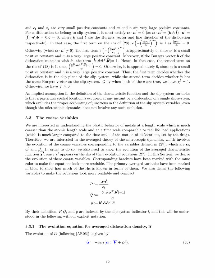
and c1 and c2 are very small positive constants and m and n are very large positive constants.For a dislocation to belong to slip system l, it must satisfy α · nl = 0 (as α · nl = (b ⊗ l) · nl =(l · nl)b = 0.b = 0, where b and l are the Burgers vector and line direction of the dislocation
respectively). In that case, the first term on the rhs of (28), e(−(|αnl|c1
)m), is 1 as |αn
l|c1
= 0.
Otherwise (when α · nl 6= 0), the first term e(−(|αnl|c1
)m)is approximately 0, since c1 is a small
positive constant and m is a very large positive constant. Moreover, if the Burgers vector b of thedislocation coincides with bl, the term |bl.ααT .bl|= 1. Hence, in that case, the second term on
the rhs of (28) is 1, since(||bl.ααT .bl|−1|
c2
)= 0. Otherwise, it is approximately 0, since c2 is a small
positive constant and n is a very large positive constant. Thus, the first term decides whether thedislocation is in the slip plane of the slip system, while the second term decides whether it hasthe same Burgers vector as the slip system. Only when both of these are true, we have χl = 1.Otherwise, we have χl ≈ 0.
An implied assumption in the definition of the characteristic function and the slip system variablesis that a particular spatial location is occupied at any instant by a dislocation of a single slip system,which excludes the proper accounting of junctions in the definition of the slip system variables, eventhough the microscopic dynamics does not involve any such exclusion.
3.3 The coarse variables
We are interested in understanding the plastic behavior of metals at a length scale which is muchcoarser than the atomic length scale and at a time scale comparable to real life load applications(which is much larger compared to the time scale of the motion of dislocations, set by the drag).Therefore, we are interested in the averaged theory of the microscopic dynamics, which involvesthe evolution of the coarse variables corresponding to the variables defined in (27), which are α,
al and ρl. In order to do so, we also need to know the evolution of the averaged characteristicfunction χl, since χl appears on the rhs of their evolution equations (27). In this Section, we derivethe evolution of these coarse variables. Corresponding brackets have been marked with the samecolor to make the equations look more readable. The primary averaged variables have been markedin blue, to show how much of the rhs is known in terms of them. We also define the followingvariables to make the equations look more readable and compact:
P :=|αnl|c1
Q :=||bl.ααT .bl|−1|
c2
p := bl.ααT .bl.
By their definition, P,Q, and p are indexed by the slip-system indicator l, and this will be under-stood in the following without explicit notation.
3.3.1 The evolution equation for averaged dislocation density, α
The evolution of α (following [AR06]) is given by
α = −curl(α× V +Lp). (30)
12

3.3.2 The evolution equation for the averaged characteristic function, χl, for slipsystem l
χl is obtained by applying the averaging operator (1) to (28). Its evolution equation is
˙χl =: Bl(state) = −m
c1e(−Pm) e(−Qn) Pm−1
[−αnl ·
curl(α× V +Lp)nl.
(1
|αnl|
)]− n
c2e(−Pm) e(−Qn) Qn−1 sgn(|p|−1) sgn(p)
bl ·
(−curl(α× V +Lp)
( 1
|α|
)+α : curl(α× V +Lp)
(1
|α|3
))αT
+ α
((−curl(α× V +Lp))T
( 1
|α|
)+α : curl(α× V +Lp)
( 1
|α|3))
· bl
− m
c1
e(−Pm) e(−Qn) Pm−1
(Σαnl · Σ−curl(α×V )nl
(1
|αnl|
)
+ Σ−(αnl)·(curl(α×V )nl) Σ1
|αnl|
)
+ Σe(−Pm) e(−Qn) Pm−1
(− 1
c1
(αnl · curl(α× V +Lp)nl
+ Σαnl · Σ−curl(α×V )nl)( 1
|αnl|
)+ Σ−(αnl)·(curl(α×V )nl) Σ
1
|αnl|
)
+ Σe(−Pm) e(−Qn) ΣPm−1
(− 1
c1
(αnl · curl(α× V +Lp)nl
+ Σαnl · Σ−curl(α×V )nl)( 1
|αnl|
)+ Σ−(αnl)·(curl(α×V )nl) Σ
1
|αnl|
)
− n
c2
[e(−Pm) e(−Qn) Qn−1
sgn(|p|−1) sgn(p) bl ·
(Σ−curl(α×V )Σ
1|α|
−[(
Σα : Σ−curl(α×V ))( 1
|α|3)
+ Σ−α:curl(α×V )Σ1|α|3α+ Σ
−α:curl(α×V )
|α|3 Σα])
αT
+ α
(Σ−(curl(α×V ))T Σ
1|α|
−[(
Σα : Σ−(curl(α×V ))T)( 1
|α|3)
+ Σ−α:(curl(α×V ))Σ1|α|3αT + Σ
−α:(curl(α×V ))
|α|3 ΣαT])
bl
13

+ sgn(|p|−1)
(Σsgn(p)Σ
bl·[(− curl(α×V )
|α| −(α:curl(α×V )
|α|3
)α)αT
+α
(− curl(α×V )T
|α| −(α:curl(α×V )
|α|3
)αT
)]bl)
+ Σsgn(|p|−1)
(Σsgn(p) bl·
[(− curl(α×V )
|α| −(α:curl(α×V )
|α|3
)α
)αT
+α
(− curl(α×V )T
|α| −(α:curl(α×V )
|α|3
)αT
)]bl)
+ Σe(−Pm) e(−Qn) Qn−1
sgn(|p|−1) sgn(p) bl ·
(−curl(α× V +Lp)
( 1
α
)+ Σ−curl(α×V )Σ
1|α|
−[(−α : curl(α× V +Lp) + Σα : Σ−curl(α×V )
)( 1
|α|3)
+ Σ−α:curl(α×V )Σ1|α|3α+ Σ
−α:curl(α×V )
|α|3 Σα])
αT
+ α
((−curl(α× V +Lp))T
( 1
α
)+ Σ−(curl(α×V ))T Σ
1|α|
−[(−α : (curl(α× V +Lp)) + ΣαT : Σ−(curl(α×V )T )
)( 1
|α|3)
+ Σ−α:(curl(α×V ))Σ1|α|3αT + Σ
−α:(curl(α×V ))
|α|3 ΣαT])
bl
+ sgn(|p|−1)
(Σsgn(p)Σ
bl·[(− curl(α×V )
|α| −(α:curl(α×V )
|α|3
)α)αT
+α
(− curl(α×V )T
|α| −(α:curl(α×V )
|α|3
)αT
)]bl)
+ Σsgn(|p|−1)
(Σsgn(p) bl·
[(− curl(α×V )
|α| −(α:curl(α×V )
|α|3
)α
)αT
+α
(− curl(α×V )T
|α| −(α:curl(α×V )
|α|3
)αT
)]bl)
+ Σe(−Pm) e(−Qn) ΣQn−1
sgn(|p|−1) sgn(p) bl ·
(−curl(α× V +Lp)
( 1
α
)+ Σ−curl(α×V )Σ
1|α|
−[(−α : curl(α× V +Lp) + Σα : Σ−curl(α×V )
)( 1
|α|3)
14

+ Σ−α:curl(α×V )Σ1|α|3α+ Σ
−α:curl(α×V )
|α|3 Σα])
αT
+ α
((−curl(α× V +Lp))T
( 1
α
)+ Σ−(curl(α×V ))T Σ
1|α|
−[(−α : (curl(α× V +Lp)) + ΣαT : Σ−(curl(α×V )T )
)( 1
|α|3)
+ Σ−α:(curl(α×V ))Σ1|α|3αT + Σ
−α:(curl(α×V ))
|α|3 ΣαT])
bl
+ sgn(|p|−1)
(Σsgn(p)Σ
bl·[(− curl(α×V )
|α| −(α:curl(α×V )
|α|3
)α)αT
+α
(− curl(α×V )T
|α| −(α:curl(α×V )
|α|3
)αT
)]bl)
+ Σsgn(|p|−1)
(Σsgn(p) bl·
[(− curl(α×V )
|α| −(α:curl(α×V )
|α|3
)α
)αT
+α
(− curl(α×V )T
|α| −(α:curl(α×V )
|α|3
)αT
)]bl)]
−m Σe(−Pm) e(−Qn) Pm−1 Σ
((αnl)·(−curl(α×V )T )nl
c1|αnl|
)
− n
(Σe(−Pm) e(−Qn) Qn−1
Σ1c2sgn(p) bl·
[− curl(α×V )
|α| +(α:curl(α×V )
|α|3 ) ααT +α
− curl(α×V )T
|α| +(α:curl(α×V )|α|3 ) αT
]bl),
(31)
where Bl(state) represents the state function given by the rhs of (31). The derivation of (31) isgiven in Appendix A.2.
3.3.3 The evolution equation for the averaged dislocation density tensor, al, for slipsystem l
al is obtained by applying the averaging operator (1) to (27a). Its evolution equation is
˙al = Bl(state) α− curl[χl (al × V )]− curl(al × ΣχlΣV ) + 2 χl (α× V )[X(gradχl)]
+ Σχ Σα − curl(
Σal × ΣV l)
+ 2 χl Σα × ΣV [X(gradχl)] + 2 Σχl Σα×V [X(gradχl)]
+ 2 Σχl(α×V ) ΣX(gradx′χl), (32)
where Bl is defined in the discussion following (31) in Section 3.3. The derivation of (32) is given
in Appendix A.3. The merit of (32) is that it shows what the exact evolution equation of al shouldbe (cf. [XEA15]). It is cumbersome, to say the least and, moreover, contains fluctuation termswhose evolution are given by other pde, resulting in an ‘unsolvable’ infinite hierarchy.
15

3.3.4 The evolution equation for the averaged total dislocation density, ρl, for slipsystem l
ρl is obtained by applying the averaging operator (1) to (27b). Its evolution is given by
˙ρl =− 2Bl(state) ρl − gradρl · (χl V ) + ρ gradχl · (χl V )− 2 ρl div(χl V ) + 2 ρl gradχl · V
+ 2 (χl α) : (αgradV ) + 2 (χl α) : (divα⊗ V )
+ 2 Σ
−m e(−Pm)e(−Qn)Pm−1
((αnl)·(−curl(α×V )T )nl
c1|αnl|
)− n
c2e(−Pm)e(−Qn)Qn−1·
sgn(p) bl·[− curl(α×V )
|α| +(α:curl(α×V )
|α|3 ) ααT +α
− curl(α×V )T
|α| +(α:curl(α×V )|α|3 ) αT
]bl
Σρl
− gradρl · Σχl ΣV + ρ gradχl · Σχl ΣV − 2 ρl div(Σχl ΣV )
− Σgradρl · ΣχlV + Σρ Σgradχl · (χl V + ΣχlΣV ) + Σρ gradχl · Σχl V − 2 Σρl Σdiv(χl V )
+ 2 Σρl Σgradχl · V + 2 Σρl gradχl · ΣV + Σχl Σα :(α gradV + Σα ΣgradV
)+ Σχlα : Σα gradV
+ 2 Σχl Σα : (divα⊗ V + Σdivα ⊗ ΣV ) + Σχlα : Σdivα⊗V
(33)
where Bl(state) is defined in the discussion following (31) in Section 3.3. The derivation of (33) is
given in Appendix A.4. The equation (33) is the exact evolution equation of ρl. The same remarksas to the practicality of this exact equation as in Section 3.3.3 applies.
Remark In the evolution equations for α (30), al (32) and ρl (33), the plastic distortion rate Lp
appears. It is defined in (13) and is a fluctuation term (Lp = Σα × ΣV ). As shown in Section2, the hierarchy can involve equations of evolution for the fluctuations. We derived the evolutionequation for Lp in (25) which is as follows:
Lp = Σ−curl(α×V ) × ΣV + Σα × ΣV .
The Lp for a uniformly expanding circular loop was obtained in Section 3.1 and is given by (26).However, this was possible due to the drastic assumption of uniform velocity (of same magnitudepointing radially outward) at all points of the loop. In reality, the value of the local velocity isdifficult to obtain without consideration of the microscopic DD problem, as it depends on the Peach-Koehler force acting on the dislocation segments, which is a function of the internal stresses. Thismakes it essentially impossible to define an evolution equation for Lp in realistic situations withoutsome sort of ‘on-the-fly’ coupling to local DD calculations. The coupled DD-MFDM strategy thatis described and implemented in [CPZ+20] defines evolution equations for Lp using appropriatetime averaging of Discrete Dislocation Dynamics is a first demonstration towards achieving exactlythis goal for realistic applied loading rates.
4 Conclusion
We stated some descriptors of the microscopic dynamics and obtained the evolution of the coarsevariables generated from such descriptors. The coarse variables give an idea of the averaged behavior
16

of the system at a much coarser length and time scale. We see that the evolution of the totaldislocation density (16) contains the averages of fluctuations, and hence is exact but not closed.We considered a refined description in which we resolved the dynamics into slip systems. We seethat the evolution of the dislocation density tensor (32) and the total dislocation density (33) ofany particular slip system is extremely cumbersome, which shows the limitations of such a refineddescription. The evolution equations of the coarse variables involve many average terms, averageof fluctuation terms and their partial derivatives, all of which have their own evolution given byother pdes. Thus, we get an infinite hierarchy of non-linear non-closed coarse evolution pdes, whichcannot be solved for all practical purposes. The CDD framework [HZG07, Hoc16, SZ15] postulatesthe microscopic dynamics and uses closure assumptions of their own to cut off the infinite hierarchyof equations. In contrast, MFDM (12), which follows by averaging the equations of FDM (11) inspace and time, is based on the fundamental statement of the conservation of Burgers vector (whichis a physically observed fact). While cumbersome, one could try to work with these exact equationsif they were known in full detail. If this is not the case, the justifications for using such infinitehierarchies is scarce. It is much more reasonable, and important to focus on closure assumptions,generated from the actual stress coupled microscopic dislocation interaction dynamics and theiraveraging, at a lower level in the hierarchy, about which such ‘kinematic’ infinite hierarchies saynothing.
In previous work starting from [AR06], the system is closed using physics-based phenomenolog-ical modeling at the lowest level of the hierarchy as a trade-off with practicality (see the dis-cussion surrounding (12), in which Lp and V are phenomenologically specified). This approachhas been quite successful in addressing a promising array of problems in modern plasticity the-ory related to the computation of patterning, dislocation internal stress, size effects, polygoniza-tion, and slip transmission at grain boundaries among others [RA06, Ach07, PRAD10, MBA10,FAB11, PAR11, PDA11, Ach11, DAS16, FBE+09, TVC+07, TBFB10, RWF11, TVFB08, DTBF15,VBF09, DBTL20, BTL20, GBG+20], including long-standing and recent fundamental challengesin the prediction of large-deformation, dislocation mediated elastic and elastic-plastic response[AA20a, AZA20, AA20b]. Despite the phenomenology, the approach has provided two distinctbenefits:
1. It is fair to say that beyond the modeling in 1 space dimension, the plastic distortion inclassical plasticity theory has, at best, only a thermodynamic physical meaning with noconcrete, tangible connection to the mechanics of dislocations. The MFDM approach based onspace-time averaging of microscopic dislocation mechanics brings out an explicit, completelydefined, connection between the plastic strain rate employed in phenomenological theoriesof plasticity and the motion and geometry of an evolving microscopic array of dislocations,as explained in the discussion surrounding (12). Obviously, this has many benefits, evenfor a phenomenological specification of the macroscopic plastic strain rate. Moreover, theMFDM framework has allowed for a first unification between phenomenological J2 and crystalplasticity theories and quantitative dislocation mechanics.
2. With a single extra material parameter beyond a classical plasticity model (and two at finitedeformations), the MFDM framework has enabled a significant variety of phenomena to bemodeled, in qualitative and quantitative accord with experimental results.
In the work presented in [CPZ+20], the phenomenological constitutive assumptions in MFDM arereplaced with inputs obtained by appropriate time averaging of Discrete Dislocation Dynamics.To our knowledge, this is the first demonstration of a coupled DD-continuum plasticity frameworkthat can be exercised at quasi-static loading rates and makes no assumptions on material response
17

beyond the elasticity of the material and a model for thermal activation of dislocations past sessilejunctions (which is not a part of the microscopic DD model). For reasons mentioned in [CPZ+20],a first systematic improvement of the DD-MFDM coupled model would be to add the equation ofthe evolution of the total density (16) to the field equations of MFDM (with its non-closed termsinvolving fluctuations supplied by local space-time averaged DD response), which would provide afurther local driving constraint (the value of ρ) to each of the local DD calculations beyond thestress of the macroscopic model. Of course, even with dropping all the fluctuation terms in (16),that equation can augment the phenomenological mode of application of MFDM, enhancing thedescription of material strength beyond the currently prevalent non-decreasing phenomenologicaldescriptions (e.g. the Voce Law). These are some of the practical benefits of pursuing the space-timeaveraged hierarchy of dislocation mechanics as developed in this paper.
Appendix A Derivation of evolution equations
A.1 Total dislocation density, ρl
From (14), we have
ρ = α : α (34)
We differentiate (34) in time to get
ρ = 2 α : α = −2 α : curl(α× V ) = −2αij [curl(α× V )]ij
= −2αijejmn(α× V )in,m = −2αijejmnenpq(αipVq),m
= −2(δjpδmq − δjqδmp)[αijαip,mVq + αijαipVq,m]
= −2[αijαij,mVm + αijαijVm,m − αijαim,mVj − αijαimVj,m]
= −2 [1
2grad(α : α) · V +α : α(divV )−α : (divα⊗ V )−α : α gradV ]
= −2 [1
2gradρ · V + ρ(divV )−α : (divα⊗ V )−α : α gradV ]
= −gradρ · V − 2ρ(divV ) + 2α : (divα⊗ V ) + 2α : α gradV (35)
We apply the averaging operator to both sides of (35) to get
ρ = −grad ρ · V − 2 ρ divV − Σgradρ · ΣV − 2ΣρΣdivV + 2 α : (divα⊗ V ) + 2 α : α gradV .(36)
Using (36) and the facts that
α : α gradV = α : α gradV +α : Σα ΣgradV + Σα : Σα gradV
α : (divα⊗ V ) = α : (divα⊗ V ) +α : (Σdivα ⊗ ΣV ) + Σα : Σdivα⊗V ,
we get the evolution of ρ as (16) in section 3.
A.2 The characteristic function, χl
We will use the following results in the derivation:
18

• If f is a vector, then
d
dt|f | = f · f
|f |, (37)
which gives,
˙|f | = f · f|f |
= f · f . 1
|f |+ Σf ·fΣ
1|f | =
(f · f + Σf · Σf
).
1
|f |+ Σf ·fΣ
1|f | . (38)
• If q is a scalar,
d
dt|q| = sgn(q)q, (39)
which gives,
˙|q| = sgn(q) q = sgn(q) q + Σsgn(q)Σq. (40)
We define
χl := e(−Pm) e(−Qn), (41)
where P = |αnl|c1
and Q = ||bl.ααT bl|−1|c2
. We also denote p = bl.ααT bl. Hence, Q = ||p|−1|c2
. Takingtime derivative of (41) and using (37) and (39), we have,
χl = −m e(−Pm)e(−Qn)Pm−1P − n e(−Pm)e(−Qn)Qn−1Q (42)
From (42), we have,
˙χl =−m
[e(−Pm) e(−Qn) Pm−1 P + Σe(−Pm) e(−Qn) Pm−1 ΣP
]− n
[e(−Pm) e(−Qn) Qn−1 Q+ Σe(−Pm) e(−Qn) Qn−1 ΣQ
]=−m e(−Pm) e(−Qn) Pm−1 P − n e(−Pm) e(−Qn) Qn−1 Q
−m Σe(−Pm) e(−Qn) Pm−1 ΣP − n Σe(−Pm) e(−Qn) Qn−1 ΣQ
=−m(e(−Pm) e(−Qn) Pm−1 + Σe(−Pm) e(−Qn) ΣPm−1
)P
− n(e(−Pm) e(−Qn) Qn−1 + Σe(−Pm) e(−Qn) ΣQn−1
)Q
−m Σe(−Pm) e(−Qn) Pm−1 ΣP − n Σe(−Pm) e(−Qn) Qn−1 ΣQ
=−m(
(e(−Pm) e(−Qn) + Σe(−Pm) e(−Qn)) Pm−1 + Σe(−Pm) e(−Qn) ΣPm−1)P
− n(
(e(−Pm) e(−Qn) + Σe(−Pm) e(−Qn)) Qn−1 + Σe(−Pm) e(−Qn) ΣQn−1)Q
−m Σe(−Pm) e(−Qn) Pm−1 ΣP − n Σe(−Pm) e(−Qn) Qn−1 ΣQ
=−m(e(−Pm) e(−Qn) Pm−1 P + Σe(−Pm) e(−Qn) Pm−1 P + Σe(−Pm) e(−Qn) ΣPm−1 P
)− n
(e(−Pm) e(−Qn) Qn−1 Q+ Σe(−Pm) e(−Qn) Qn−1 Q+ Σe(−Pm) e(−Qn) ΣQn−1 Q
)−m Σe(−Pm) e(−Qn) Pm−1 ΣP − n Σe(−Pm) e(−Qn) Qn−1 ΣQ
(43)
19

From the definition of P in the discussion following (41) and using (37),
P =1
c1
(α nl) · (α nl)|α nl|
= − 1
c1
(α nl) · curl(α× V ) nl|α nl|
(44)
Using (38),
P =1
c1
[(αnl · ˙
αnl + Σαnl · Σαnl)( 1
|αnl|
)+ Σ(αnl)·(αnl) Σ
1
|αnl|
]
=1
c1
[((αnl) · (αnl) + Σαnl · Σαnl
)( 1
|αnl|
)+ Σ(αnl)·(αnl) Σ
1
|αnl|
]
=1
c1
[(− (αnl) · (curl(α× V +Lp)nl) + Σαnl · Σαnl
)( 1
|αnl|
)+ Σ−(αnl)·(curl(α×V )nl) Σ
1
|αnl|]. (45)
From the definition of p and Q in the discussion following (41) and using (39),
Q =1
c2sgn(|p|−1) sgn(p) p =
1
c2sgn(|p|−1) sgn(p) bl · ( ˙ααT + α ˙αT )bl (46)
Now,
˙α =α
|α|−(α : α
|α|3
)α = −curl(α× V )
|α|+
(α : curl(α× V )
|α|3
)α
˙αT =αT
|α|= −curl(α× V )T
|α|+
(α : curl(α× V )
|α|3
)αT (47)
Substituting (47) into (46),
Q =1
c2sgn(|p|−1) sgn(p) bl ·
[− curl(α× V )
|α|+ (α : curl(α× V )
|α|3) ααT
+ α− curl(α× V )T
|α|+ (α : curl(α× V )
|α|3) αT
]bl (48)
Using (46),
Q =1
c2sgn(|p|−1) sgn(p) p =
1
c2
[sgn(|p|−1) sgn(p) p+ Σsgn(|p|−1)Σsgn(p)p
]=
1
c2
[sgn(|p|−1)
sgn(p) p+ Σsgn(p)Σp
+ Σsgn(|p|−1)Σsgn(p)p
]=
1
c2
[sgn(|p|−1) sgn(p) p+ sgn(|p|−1) Σsgn(p)Σp + Σsgn(|p|−1)Σsgn(p)p
] (49)
Using the definition of p in the discussion around (46) ,
p = bl · ( ˙ααT + α ˙αT )bl
20

=⇒ p = bl · ( ˙α αT + α˙αT )bl (50)
Following (12), we have
α = −curl(α× V +Lp)
From (47),
˙α =
(α
1
|α|+ ΣαΣ
1|α|
)−
(α : α
|α|3
)α+ Σ
α:α|α|3 Σα
=
(α
1
|α|+ ΣαΣ
1|α|
)−
(α : α
|α|3
)α+ Σ
α:α|α|3 Σα
=
(α
1
|α|+ ΣαΣ
1|α|
)−[(
α : α+ Σα : Σα) 1
|α|3+ Σα:αΣ
1|α|3
α+ Σ
α:α|α|3 Σα
]=(−curl(α× V +Lp)
1
|α|+ Σ−curl(α×V )Σ
1|α|)−
[(−α : curl(α× V +Lp)
+ Σα : Σ−curl(α×V )) 1
|α|3+ Σα:−curl(α×V )Σ
1|α|3
α+ Σ
−α:curl(α×V )
|α|3 Σα
]. (51)
Similarly, we can obtain˙αT = αT
|α| by replacing α, α, α and α above with their respective transposeand obtain
˙αT =
((−curl(α× V +Lp))T
1
|α|+ Σ−(curl(α×V ))T Σ
1|α|)−
[(−α : (curl(α× V +Lp))
+ ΣαT : Σ−(curl(α×V ))T) 1
|α|3+ Σ−α:(curl(α×V ))Σ
1|α|3
αT + Σ
−α:(curl(α×V ))
|α|3 ΣαT
]. (52)
Using (49), (50), (51) and (52), we get
Q =1
c2sgn(|p|−1) sgn(p) bl ·
(−curl(α× V +Lp)
( 1
α
)+ Σ−curl(α×V )Σ
1|α|
−[(−α : curl(α× V +Lp) + Σα : Σ−curl(α×V )
)( 1
|α|3)
+ Σ−α:curl(α×V )Σ1|α|3α+ Σ
−α:curl(α×V )
|α|3 Σα])
αT
+ α
((−curl(α× V +Lp))T
( 1
α
)+ Σ−(curl(α×V ))T Σ
1|α|
−[(−α : (curl(α× V +Lp)) + ΣαT : Σ−(curl(α×V )T )
)( 1
|α|3)
+ Σ−α:(curl(α×V ))Σ1|α|3αT + Σ
−α:(curl(α×V ))
|α|3 ΣαT])
bl
21

+1
c2sgn(|p|−1)
(Σsgn(p)Σ
bl·[(− curl(α×V )
|α| −(α:curl(α×V )
|α|3
)α)αT
+α
(− curl(α×V )T
|α| −(α:curl(α×V )
|α|3
)αT
)]bl)
+1
c2Σsgn(|p|−1)
(Σsgn(p) bl·
[(− curl(α×V )
|α| −(α:curl(α×V )
|α|3
)α
)αT
+α
(− curl(α×V )T
|α| −(α:curl(α×V )
|α|3
)αT
)]bl)
(53)
Using (42), (45), (46), (50), (51) and (52), we get the evolution of χl given by (31) in section3.
A.3 Dislocation density tensor corresponding to slip system l, al
Following (27), the dislocation density corresponding to slip system l is defined as
al := χlα. (54)
We take time derivative of (54) to obtain
al = χlα+ χlα
= χlα− χlcurl(α× V ).
(55)
Using the fact that χl ≈ (χl)2, since χl can (approximately) take either of the values 0 or 1, thesecond term on the right hand side above can be written as
χlcurl(α× V ) = χlcurl(α× V )im ≈ (χl)2emjkα× V ik,j
= emjkχlα× χlV ik,j − emjkα× V ik∂χl
2
∂χj′
= curl(χlα× χlV)im − 2α× V ikemjkχl∂χl
∂χj′
= curl(al × V l)im − 2 χl α× V ik[X(gradx′χl)]km
⇒ χlcurl(α× V ) = curl(al × V l)− 2 χl(α× V )[X(gradx′χl)], (56)
where emjk is a component of the third-order alternating tensor X and its action on a tensor A isgiven by X(A)i = eijkAjk, while its action on a vector N is given by X(N)ij = eijkNk.
Using (55) and (56) above, we have
al = χlα− curl(al × V l) + 2 χl(α× V )[X(gradx′χl)]. (57)
22

We average both sides of (57) to get
˙al =
˙χl α+ Σχl Σα − curl(al × V l)− curl
(Σal × ΣV l
)+ 2χl(α× V )[X(gradx′χl)] (58)
We have
2χl(α× V )[X(gradx′χl)] = 2 χl(α× V ) [X(gradχl)] + 2 Σχl(α×V ) ΣX(gradx′χl)
= 2(χl α× V + Σχl Σα×V
)[X(gradχl)] + 2 Σχl(α×V ) ΣX(gradx′χ
l)
= 2 χl (α× V )[X(gradχl)] + 2 χl Σα × ΣV [X(gradχl)] + 2 Σχl Σα×V [X(gradχl)]
+ 2 Σχl(α×V ) ΣX(gradx′χl)
Hence, using (58), we have
˙al =
˙χl α+ Σχ Σα − curl(al × V l)− curl
(Σal × ΣV l
)+ 2 χl (α× V )[X(gradχl)] + 2 χl Σα × ΣV [X(gradχl)] + 2 Σχl Σα×V [X(gradχl)]
+ 2 Σχl(α×V ) ΣX(gradx′χl) (59)
Finally, we use (42) and (31) to obtain the evolution of al as (32) in section 3.
A.4 Total dislocation density corresponding to slip system l, ρl
The total dislocation density corresponding to slip system l is defined in (27) and is given by
ρl := al : al = (χlα) : (χlα) ≈ (χl)2 α : α. (60)
We differentiate (60) with respect to time to get
ρl = 2χl χl α : α+ 2 (χl)2 α : α
= 2χlρl + χl[2α : α].
Using (35), we have,
ρl = 2χlρl − 2χl[1
2gradρ · V + ρ(divV )−α : α gradV −α : (divα⊗ V )
]≈ 2χlρl − (χl)2gradρ · V − 2(χl)2ρ divV + 2χlα : (α gradV ) + 2χlα : (divα⊗ V )
= 2χlρl − χlgradρ · (χlV )− 2(χlρ)χl divV + 2χlα : (α gradV ) + 2χlα : (divα⊗ V )
= 2χlρl − gradρl − ρ gradχl · V l − 2ρldivV l − gradχl · V + 2χlα : (α gradV ) + 2χlα : (divα⊗ V )
= 2χlρl − gradρl · V l + ρ gradχl · V l − 2ρldivV l + 2ρlgradχl · V+ 2χlα : (α gradV ) + 2χlα : (divα⊗ V ). (61)
We average both sides of (61) to get the evolution of ρl as
˙ρl = 2
˙χl ρl + 2Σχl Σρl − gradρl · V l − Σgradρl · ΣV l + ρ gradχl · V l + Σρ gradχl · ΣV l
23
− 2 ρl divV l − 2 Σρl ΣdivV l + 2 ρl gradχl · V + 2 Σρl gradχl · ΣV
+ 2 χlα : (α gradV ) + 2 χlα : (divα⊗ V ) (62)
Also,
χlα : (α gradV ) = χlα : α gradV + Σχlα : Σα gradV
= (χl α+ Σχl Σα) : (α gradV + Σα ΣgradV ) + Σχlα : Σα gradV
Similarly,
χlα : (divα⊗ V ) = χlα : divα⊗ V + Σχlα : Σdivα⊗V
= (χl α+ Σχl Σα) : (divα⊗ V + Σdivα ⊗ ΣV ) + Σχlα : Σdivα⊗V
Hence,
˙ρl = 2
˙χl ρl + 2Σχl Σρl − gradρl · V l − Σgradρl · ΣV l + ρ gradχl · V l + Σρ Σgradχl · V l
+ Σρ gradχl · ΣV l − 2 ρl divV l − 2 Σρl ΣdivV l + 2 ρl gradχl · V + 2 Σρl Σgradχl · V
+ 2 Σρl gradχl · ΣV +(χl α+ Σχl Σα
):(α gradV + Σα ΣgradV
)+ Σχlα : Σα gradV
+ 2 (χl α+ Σχl Σα) : (divα⊗ V + Σdivα ⊗ ΣV ) + Σχlα : Σdivα⊗V
=⇒ ˙ρl = 2
˙χl ρl − gradρl · V l + ρ gradχl · V l − 2 ρl divV l + 2 ρl gradχl · V
+ 2 (χl α) : (αgradV ) + 2 (χl α) : (divα⊗ V ) + 2Σχl Σρl − Σgradρl · ΣV l
+ Σρ Σgradχl · V l + Σρ gradχl · ΣV l − 2 Σρl ΣdivV l + 2 Σρl Σgradχl · V
+ 2 Σρl gradχl · ΣV + Σχl Σα :(α gradV + Σα ΣgradV
)+ Σχlα : Σα gradV
+ 2 Σχl Σα : (divα⊗ V + Σdivα ⊗ ΣV ) + Σχlα : Σdivα⊗V
(63)
Finally, using (42) and (31), we have the evolution equation for ρl as (33) in section 3.
Acknowledgment
Support from NSF grant NSF-CMMI-1435624 is gratefully acknowledged.
References
[AA20a] Rajat Arora and Amit Acharya. Dislocation pattern formation in finite deformationcrystal plasticity. International Journal of Solids and Structures, 184:114–135, 2020.
[AA20b] Rajat Arora and Amit Acharya. A unification of finite deformation J2 von-Mises plas-ticity and quantitative dislocation mechanics. Journal of the Mechanics and Physics ofSolids, page 104050, 2020.
24
[AC12] Amit Acharya and S. Jonathan Chapman. Elementary observations on the averagingof dislocation mechanics: dislocation origin of aspects of anisotropic yield and plasticspin. Procedia IUTAM, 3:297–309, 2012.
[Ach01] Amit Acharya. A model of crystal plasticity based on the theory of continuously dis-tributed dislocations. Journal of the Mechanics and Physics of Solids, 49(4):761 – 784,2001.
[Ach03] Amit Acharya. Driving forces and boundary conditions in continuum dislocation me-chanics. Proceedings of the Royal Society of London. Series A: Mathematical, Physicaland Engineering Sciences, 459, 2003.
[Ach04] Amit Acharya. Constitutive analysis of finite deformation field dislocation mechanics.Journal of the Mechanics and Physics of Solids, 52(2):301 – 316, 2004.
[Ach07] Amit Acharya. Jump condition for GND evolution as a constraint on slip transmissionat grain boundaries. Philosophical magazine, 87(8-9):1349–1359, 2007.
[Ach11] Amit Acharya. Microcanonical entropy and mesoscale dislocation mechanics and plas-ticity. Journal of Elasticity, 104(1-2):23–44, 2011.
[AR06] Amit Acharya and Anish Roy. Size effects and idealized dislocation microstructure atsmall scales: Predictions of a phenomenological model of mesoscopic field dislocationmechanics: Part I. Journal of the Mechanics and Physics of Solids, 54:1687–1710, 2006.
[AZA20] Rajat Arora, Xiaohan Zhang, and Amit Acharya. Finite element approximation offinite deformation dislocation mechanics. Computer Methods in Applied Mechanics andEngineering, 367:113076, 2020.
[Bab97] Marijan Babic. Average balance equations for granular materials. International Journalof Engineering Science, 35(5):523 – 548, 1997.
[BTL20] Stephane Berbenni, Vincent Taupin, and Ricardo A Lebensohn. A fast Fouriertransform-based mesoscale field dislocation mechanics study of grain size effects andreversible plasticity in polycrystals. Journal of the Mechanics and Physics of Solids,135:103808, 2020.
[CPZ+20] Sabyasachi Chatterjee, Giacomo Po, Xiaohan Zhang, Amit Acharya, and Nasr Ghoniem.Plasticity without phenomenology: a first step. Journal of the Mechanics and Physicsof Solids, 143:104059, 2020.
[DAS16] Amit Das, Amit Acharya, and Pierre Suquet. Microstructure in plasticity withoutnonconvexity. Computational Mechanics, 57(3):387–403, 2016.
[DBTL20] Komlan S Djaka, Stephane Berbenni, Vincent Taupin, and Ricardo A Lebensohn. AFFT-based numerical implementation of mesoscale field dislocation mechanics: appli-cation to two-phase laminates. International Journal of Solids and Structures, 184:136–152, 2020.
[DTBF15] KS Djaka, Vincent Taupin, Stephane Berbenni, and Claude Fressengeas. A numericalspectral approach to solve the dislocation density transport equation. Modelling andSimulation in Materials Science and Engineering, 23(6):065008, 2015.
[FAB11] Claude Fressengeas, A Acharya, and Armand Joseph Beaudoin. Dislocation medi-ated continuum plasticity: Case studies on modeling scale dependence, scale-invariance,
25
and directionality of sharp yield-point. In Computational Methods for Microstructure-Property Relationships, pages 277–309. Springer, 2011.
[FBE+09] C Fressengeas, Armand Joseph Beaudoin, Denis Entemeyer, T Lebedkina, M Lebyodkin,and V Taupin. Dislocation transport and intermittency in the plasticity of crystallinesolids. Physical Review B, 79(1):014108, 2009.
[GAM15] Akanksha Garg, Amit Acharya, and Craig E. Maloney. A study of conditions for dislo-cation nucleation in coarser-than-atomistic scale models. Journal of the Mechanics andPhysics of Solids, 75:76 – 92, 2015.
[GBG+20] J Genee, S Berbenni, N Gey, Ricardo A Lebensohn, and F Bonnet. Particle inter-spacing effects on the mechanical behavior of a fe–tib 2 metal matrix composite usingfft-based mesoscopic field dislocation mechanics. Advanced Modeling and Simulation inEngineering Sciences, 7(1):1–23, 2020.
[Hoc16] Thomas Hochrainer. Thermodynamically consistent continuum dislocation dynamics.Journal of the Mechanics and Physics of Solids, 88:12 – 22, 2016.
[HZG07] T. Hochrainer, M. Zaiser, and P. Gumbsch. A three-dimensional continuum theory ofdislocation systems: kinematics and mean-field formulation. Philosophical Magazine,87(8-9):1261–1282, 2007.
[KAA75] U.F. Kocks, A.S. Argon, and M.F. Ashby. Thermodynamics and Kinetics of Slip.Progress in materials science. Pergamon Press, 1975.
[MBA10] Justin C Mach, Armand J Beaudoin, and Amit Acharya. Continuity in the plastic strainrate and its influence on texture evolution. Journal of the Mechanics and Physics ofSolids, 58(2):105–128, 2010.
[MZ18] Mehran Monavari and Michael Zaiser. Annihilation and sources in continuum disloca-tion dynamics. Materials Theory, 2:3, 2018.
[PAR11] Saurabh Puri, Amit Acharya, and Anthony D Rollett. Controlling plastic flow acrossgrain boundaries in a continuum model. Metallurgical and Materials Transactions A,42(3):669–675, 2011.
[PDA11] Saurabh Puri, Amit Das, and Amit Acharya. Mechanical response of multicrystallinethin films in mesoscale field dislocation mechanics. Journal of the Mechanics and Physicsof Solids, 59(11):2400–2417, 2011.
[PRAD10] Saurabh Puri, Anish Roy, Amit Acharya, and Dennis Dimiduk. Modeling dislocationsources and size effects at initial yield in continuum plasticity. Journal of Mechanics ofMaterials and Structures, 4(9):1603–1618, 2010.
[RA06] Anish Roy and Amit Acharya. Size effects and idealized dislocation microstructure atsmall scales: predictions of a phenomenological model of mesoscopic field dislocationmechanics: Part II. Journal of the Mechanics and Physics of Solids, 54(8):1711–1743,2006.
[RWF11] T Richeton, GF Wang, and C28678661270 Fressengeas. Continuity constraints at in-terfaces and their consequences on the work hardening of metal–matrix composites.Journal of the Mechanics and Physics of Solids, 59(10):2023–2043, 2011.
26
[SHZG11] Stefan Sandfeld, Thomas Hochrainer, Michael Zaiser, and Peter Gumbsch. Continuummodeling of dislocation plasticity: Theory, numerical implementation, and validationby discrete dislocation simulations. Journal of Materials Research, 26(5):623–632, 2011.
[SZ15] Stefan Sandfeld and Michael Zaiser. Pattern formation in a minimal model of continuumdislocation plasticity. Modelling and Simulation in Materials Science and Engineering,23(6):065005, 2015.
[TBFB10] V Taupin, S Berbenni, C Fressengeas, and O Bouaziz. On particle size effects: Aninternal length mean field approach using field dislocation mechanics. Acta Materialia,58(16):5532–5544, 2010.
[TVC+07] V Taupin, S Varadhan, J Chevy, C Fressengeas, Armand Joseph Beaudoin, MaurineMontagnat, and Paul Duval. Effects of size on the dynamics of dislocations in ice singlecrystals. Physical review letters, 99(15):155507, 2007.
[TVFB08] V Taupin, S Varadhan, C Fressengeas, and AJ Beaudoin. Directionality of yield pointin strain-aged steels: the role of polar dislocations. Acta materialia, 56(13):3002–3010,2008.
[VBF09] S Varadhan, Armand Joseph Beaudoin, and C Fressengeas. Lattice incompatibilityand strain-ageing in single crystals. Journal of the Mechanics and Physics of Solids,57(10):1733–1748, 2009.
[XEA15] Shengxu Xia and Anter El-Azab. Computational modelling of mesoscale dislocationpatterning and plastic deformation of single crystals. Modelling Simul. Mater. Sci. Eng,23, 2015.
[ZCA13] Y. Zhu, S.J. Chapman, and A. Acharya. Dislocation motion and instability. Journal ofthe Mechanics and Physics of Solids, 61:1835–1853, 2013.
27