how much does household collateral constrain regional risk

How Much Does Household Collateral

Constrain Regional Risk Sharing?

Hanno Lustig∗

UCLA and NBER

Stijn Van Nieuwerburgh†

NYU Stern and NBER

September 20, 2006

Abstract

We construct a new data set of consumption and income data for the largest US metropol-

itan areas, and we show that the covariance of regional consumption and income growth varies

over time and in the cross-section. In times and regions where collateral is scarce, regional con-

sumption growth is about twice as sensitive to income growth. Household-level borrowing fric-

tions can explain this new stylized fact. When the value of housing relative to human wealth

falls, loan collateral shrinks, borrowing (risk-sharing) declines, and the sensitivity of con-

sumption to income increases. Our model aggregates heterogeneous, borrowing-constrained

households into regions characterized by a common housing market. The resulting regional

consumption patterns quantitatively match those in the data.

∗email:[email protected], Dept. of Economics, UCLA, Box 951477 Los Angeles, CA 90095-1477†email: [email protected], Dept. of Finance, NYU, 44 West Fourth Street, Suite 9-120, New York, NY

10012. First version May 2002. The material in this paper circulated earlier as ”Housing Collateral and Risk SharingAcross US Regions.” (NBER Working Paper). The authors thank Thomas Sargent, David Backus, Dirk Krueger,Patrick Bajari, Timothey Cogley, Marco Del Negro, Robert Hall, Lars Peter Hansen, Patrick Kehoe, Martin Lettau,Sydney Ludvigson, Fabrizio Perri, Luigi Pistaferri, Laura Veldkamp, Pierre-Olivier Weill, and Noah Williams. Wealso benefited from comments from seminar participants at various institutions. Keywords: Regional risk sharing,housing collateral, JEL F41,E21

1 Introduction

The cross-sectional correlation of consumption in US metropolitan areas is much smaller than the

correlation of labor income or output. This quantity anomaly has previously been documented in

international (e.g. Backus, Kehoe and Kydland (1992), and Lewis (1996)) and in state-level data

(e.g. Atkeson and Bayoumi (1993), Hess and Shin (2000) and Crucini (1999)). However, the un-

conditional moments hide a surprising amount of variation in the cross-correlation of consumption

over time. This novel dimension of the quantity anomaly is the focus of this paper. We use a new

data set of US metropolitan areas to establish this fact and we propose a new housing collateral

model to explain it.

On average, US metropolitan areas share only a modest fraction of region-specific income risk.

But this fraction varies substantially over time. The dashed line in Figure 1 plots the ratio of

the regional cross-sectional consumption to income dispersion, a standard measure of risk sharing.

This measure fell by half between 1978 and 1988, while it doubled between 1988 and 1995 before

falling back to its 1988 level in 2002. This stylized fact presents a new challenge to standard

models, because it reveals that the departures from complete market allocations fluctuate over

time. Conditioning on a measure of housing collateral helps to understand this aspect of the

consumption correlation puzzle. Our empirical measure of housing collateral scarcity broadly tracks

the variation in this regional consumption-to-income dispersion ratio. It is close to its highest level

in 1978, falls by half between 1978 and 1988, increases again until 1996, and falls back to its 1988

level in 2002. According to our estimates, the fraction of regional income risk that is traded away,

more than doubles when we compare the lowest to the highest collateral scarcity period in postwar

US data.

[Figure 1 about here.]

We propose an equilibrium model of household risk sharing that reproduces the time-variation

in regional risk sharing as well as the quantity anomaly. The model adds a regional dimension to

the model of Lustig and Van Nieuwerburgh (2005a), a crucial extension to generate the quantity

anomaly. Within each region, households face a stochastic income process that has a household-

specific and a region-specific component. What prevents perfect consumption insurance is that

households can share income risk only to the extent that borrowing is collateralized by housing

wealth. Human wealth is not collateralizable. The key ingredient for replicating the quantity anom-

aly is that borrowing constraints operate at the household level. Such constraints are much tighter

than the constraints that would be faced by a stand-in agent at the regional level. Because there

is some intra-regional risk-sharing, household consumption, as a share of regional consumption,

is less negatively correlated than household income within a region. Aggregation to the regional

level produces inter-regional consumption growth dispersion that exceeds regional income growth

1

dispersion, at least when risk sharing is small. The key ingredient for replicating the time-variation

is variation in the value of housing collateral. Variation in the housing supply and the equilibrium

house price shift the effectiveness of the household risk sharing technology over time. A reduction

in the value of housing collateral tightens the household collateral constraints, causing regional con-

sumption growth to respond more to regional income shocks. The ratio of income-to-consumption

dispersion increases as collateral becomes scarcer.

The null hypothesis of perfect insurance is usually tested by projecting regional consumption

growth on income growth. The collateral effect in our model introduces an interaction term of

region-specific income growth with housing collateral scarcity. According to the theory, the sign on

this interaction term should be positive. When collateral is scarce, a shock to region-specific income

leads to a larger change in region-specific consumption. We run this linear regression on actual

data and on data generated by our calibrated model. In the actual data, the sign on the interaction

term is positive and measured precisely. The housing collateral effect is economically significant.

Housing collateral scarcity in the 95th percentile of the empirical distribution is associated with

35% of region-specific income shocks being shared, while collateral scarcity in the 5th percentile

level corresponds to regions sharing 92% of income risk. The same regression on model-generated

data for consumption and income replicates these results. The advantage of this risk-sharing test,

based on the interaction effect of the collateral measure and income growth, is that is more specific

than the standard regression, and the appropriate test for our collateral model. There is evidence

from the cross-section as well. The income elasticity of consumption growth doubles in the quartile

of regions with the least collateral, compared to those regions in the highest quartile.

The rest of the paper is organized as follows. Section 2 sets up the model, characterizes

equilibrium allocations and prices, calibrates, and computes it. Section 3 describes the data and

compares the results from the linear consumption growth regressions in the model and in the data.

Section 4 presents additional evidence for the housing collateral mechanism. We find similar results

for Canadian provinces and find that there is also a positive relationship between the degree of

risk sharing and regional measures of collateral. Section 5 concludes.

2 A Theory of Time-Varying Risk Sharing

In this section we provide a model that replicates two key features of the observed regional con-

sumption and income distribution. First, the average ratio of the cross-sectional consumption

dispersion to income dispersion is larger than one, i.e. the quantity anomaly. Second, this ratio

increases as collateral becomes scarcer.

The model is a dynamic general equilibrium model that approximates the modest frictions

inhibiting perfect risk-sharing in advanced economies like the US. The model is based on two

2

ideas: that debts can only be enforced to the extent that they can be collateralized, and that the

primary source of collateral is housing. Our emphasis on housing, rather than financial assets,

reflects three features of the US economy: the participation rate in housing markets is very high

(2/3 of households own their home), the value of the residential real estate makes up over seventy-

five percent of total assets for the median household (Survey of Consumer Finances, 2001), and

housing is a prime source of collateral.

We relax the assumption in the Lucas (1978) endowment economy that contracts are perfectly

enforceable, following Alvarez and Jermann (2000), and allow households to file for bankruptcy,

following Lustig (2003). Each household owns part of the housing stock. Housing provides both

utility services and collateral services. When a household chooses not to honor its debt repayments,

it loses all housing collateral but its labor income is protected from creditors. Defaulting house-

holds regain immediate access to credit markets. The lack of commitment gives rise to collateral

constraints whose tightness depends on the relative abundance of housing collateral. As a result,

the effectiveness of the household risk sharing technology endogenously varies over time due to

movements in the value of housing collateral.1

The section starts with a description of the environment in 2.1 and market structure in 2.2. We

then provide a characterization of equilibrium allocations in section 2.3. The model gives rise to

a simple, non-linear risk-sharing rule. The model has two levels of heterogeneity: households and

regions. The key friction, collateralized borrowing, operates at the household level. We construct

regional consumption and income by aggregating across households in a region. We show in 2.4

that the household collateral constraints give rise to tighter constraints at the regional level than

those that would arise if there was a representative agent in each region. Section 2.5 calibrates

the model and section 2.6 explains the computational procedure. Section 2.7 simulates the model.

It shows that the aggregation from the household to the regional level generates the quantity

anomaly at the regional level. In the next section, we use the same simulated data to estimate

linear consumption growth regressions at the regional level.

2.1 Uncertainty, Preferences and Endowments

We consider an economy with a continuum of regions. There are two types of infinitely lived

households in each of these regions, and households cannot move between regions.

Uncertainty There are three layers of uncertainty: an event s consists of x, y, and z. We use

st to denote the history of events st = (xt, yt, zt), where xt ∈ X t denotes the history of household

events, yt ∈ Y t denotes the history of regional events and zt ∈ Zt denotes the history of aggregate

1Ortalo-Magne and Rady (1998), Ortalo-Magne and Rady (1999) and Pavan (2005) have also developed modelsthat deliver this feature.

3

events. π(st|s0) denotes the probability of history st, conditional on observing s0.

The household-level event x is first-order Markov, and the x shocks are independently and

identically (henceforth i.i.d.) distributed across regions. In our calibration below, x takes on one

of two values, high (hi) or low (lo). When x = hi, the first household in that region is in the high

state, and, the second household is in the low state. When x = lo, the first household is in the

low state. The region-level event y is also first-order Markov and it is i.i.d. across regions. We will

appeal to a law of large numbers (LLN) when integrating across households in different regions.2

Preferences The households j in each region i rank consumption plans consisting of (non-

durable) non-housing consumption{cijt (st)

}and housing services

{hij

t (st)}

according to the ob-

jective function in equation (1).

U(c, h) =∑

st|s0

∞∑t=0

βtπ(st|s0)u(ct(st), ht(s

t)), (1)

where β is the time discount factor, common to all regions. The households have power utility

over a CES-composite consumption good:

u(ct, ht) =1

1− γ

[c

ε−1ε

t + ψhε−1

εt

] (1−γ)εε−1

,

The preference parameter ψ > 0 converts the housing stock into a service flow, γ is the coefficient

of relative risk aversion, and ε is the intra-temporal elasticity of substitution between non-durable

and housing services consumption.3

Endowments Each of the households, indexed by j, in a region, indexed by i, is endowed with

a claim to a labor income stream{ηij

t (xt, yt, zt)

}. The aggregate non-housing endowment {ηa

t (zt)}

is the sum of the household endowments in all regions:

ηat (z

t) =∑yt

πz(yt)ηit(yt, z

t)

where πz(yt) denotes the fraction of regions that draws aggregate state z. Likewise, the regional

non-housing endowment {ηit(yt, z

t)} is the sum of the individual endowments of the households in

2The usual caveat applies when applying the LLN; we implicitly assume the technical conditions outlined byUhlig (1996) are satisfied.

3These preferences belong to the class of homothetic power utility functions of Eichenbaum and Hansen (1990).The special case of separability corresponds to γε = 1.

4

that region:

ηit(yt, z

t) =∑j=1,2

ηijt (xt, yt, z

t).

The left hand side does not depend on xt, because the two household endowments always sum to

the regional endowment, regardless of whether the first household is in the high or the low state.

Each region i receives a share of the aggregate non-housing endowment denoted by ηit(yt, zt) À

0. Thus, regional income shares are defined as in the empirical section: ηit(yt, zt) =

ηit(yt,zt)

ηat (zt)

.

Household j’s labor endowment share in region i, measured as a fraction of the regional endowment

share, is denoted ˆηjt (xt) À 0. The shares add up to one within each region: ˆη1

t (xt) + ˆη2t (xt) = 1.

The level of the labor endowment of household j in region i can be written as:

ηijt (xt, yt, z

t) = ˆηjt (xt)η

it(yt, zt)η

at (z

t).

In addition, each region is endowed with a stochastic stream of non-negative housing services

χit(y

t, zt) À 0. In contrast to non-housing consumption, the housing services cannot be transported

across regions. We will come back to the assumptions we make on χi at the end of section 2.3. So

far, we have made the following assumptions about the endowment processes:

Assumption 1. The household-specific labor endowment share ˆηj only depends on xt. The regional

income share ηit only depends on (yt, zt). The events (x, y, z) follow a first-order Markov process.

2.2 Trading

We set up an Arrow-Debreu economy where all trade takes place at time zero, after observing the

initial state s0.4 We denote the present discounted value of any endowment stream {d} after a

history st as Πst [{dτ (sτ )}], defined by

∑sτ |st

∑∞τ=t [pτ (sτ |st) dτ (sτ |st)], where pt(s

t) denotes the

Arrow-Debreu price of a unit of non-housing consumption in history st.

Households in each region purchase a complete, state-contingent consumption plan

{cijt (θij

0 , st), hijt (θij

0 , st)}∞

t=0

where θij0 denotes initial non-labor wealth.5 They are subject to a single time zero budget constraint

which states that the present discounted value of non-housing and housing consumption must not

4The same allocation can also be decentralized with sequential trade.5θij

0 denotes the value of household j’s initial claim to housing wealth, as well as any other financial wealth thatis in zero net aggregate supply. We refer to this as non-labor wealth. The initial distribution of non-labor wealth isdenoted Θ0.

5

exceed the present discounted value of the labor income stream and the initial non-labor wealth:

Πs0

[{cijt (θij

0 , st) + ρi(st)hijt (θij

0 , st)}]

6 θij0 + Πs0

[{ηij

0 (st)}]

, (2)

Collateral Constraints In this time-zero-trading economy, collateral constraints restrict the

value of a household’s consumption claim net of its labor income claim to be non-negative:

Πst

[{cijτ (θij

0 , sτ ) + ρiτ (s

τ )hijτ (θij

0 , sτ )}] ≥ Πst

[{ηij

τ (xτ , yτ , zτ )

}]. (3)

The left hand side denotes the value of adhering to the contract following node st; the right hand

side the value of default. Default implies the loss of all housing collateral wealth, and a fresh start

with the present value of future labor income. The households in each region are subject to a

sequence of collateral constraints, one for each future state sτ . These constraints are not too tight,

in the sense of Alvarez and Jermann (2000), in an environment where agents cannot be excluded

from trading.6

These constraints differ from the typical solvency constraints that decentralize constrained

efficient allocations in environments with exclusion from trading upon default.7

Definition 1. A Kehoe-Levine equilibrium is a list of allocations {cijt (θij

0 , st)}, {hijt (θij

0 , st)} and

prices {ρit(s

t)}, {pt(st)} such that, for a given initial distribution Θ0 over non-labor wealth holdings

and initial states (θ0, s0), (i) the allocations solve the household problem, (ii) the markets clear in

all states of the world:

Consumption markets clear for all t, zt:

∑j=1,2

∑

xt,yt

∫cijt (θij

0 , xt, yt, zt)π(xt, yt, zt|x0, y0, z0)

π(zt|z0)dΘ0 = ηa

t (zt)

Housing markets in each region i clear for all t, xt, yt, zt:

∑j=1,2

hijt (θij

0 , xt, yt, zt) = χit(y

t, zt).

6See Lustig (2003) for a formal proof.7Most other authors in this literature take the outside option upon default to be exclusion from future participa-

tion in financial markets (e.g. Kehoe and Levine (1993), Krueger (2000), Krueger and Perri (2006), and Kehoe andPerri (2002))If we imposed exclusion from trading instead, the solvency constraints would be looser on average, butthe same mechanism would operate. The reason is that in autarchy the household would still have to buy housingservices with its endowment of non-housing goods. An increase in the relative price of housing services would worsenthe outside option and loosen the solvency constraints, as it does in our model.

6

2.3 Equilibrium Allocations

To characterize the equilibrium consumption dynamics we use stochastic consumption weights

that describe the consumption of each household as a fraction of the aggregate endowment (see

appendix A for a complete derivation). Instead of solving a social planner problem, we characterize

equilibrium allocations and prices directly off the household’s necessary and sufficient first order

conditions. The household problem is a standard convex problem: the objective function is concave

and the constraint set is convex. In equilibrium, for any two households j and j′ in any two regions

i and i′, the level of marginal utilities satisfies:

ξijt+1uc(c

ijt+1(θ

ij0 , st, s′), hij

t+1(θij0 , st, s′)) = ξi′j′

t+1uc(ci′j′t+1(θ

i′j′0 , st, s′), hi′j′

t+1(θi′j′0 , st, s′)),

at any node (st, s′), where ξij is the consumption weight of household j in region i. Our model

provides an equilibrium theory of these consumption weights. We focus here on equilibrium al-

locations in the model where preferences over non-durable consumption and housing services are

separable (γε = 1), but all results carry over to the case of non-separability.

Cutoff Rule The equilibrium dynamics of the consumption weights are non-linear. They follow

a simple cutoff rule, which follows from the first order conditions of the constrained optimization

problem. The weights start off at ξij0 = νij at time zero; this initial weight is the multiplier on

the initial promised utility constraints. The new weight ξijt of a generic household ij that enters

period t with weight ξijt−1 equals the old weight as long as the household does not switch to a state

with a binding collateral constraint. When a household enters a state with a binding constraint,

its new weight ξijt is re-set to a cutoff weight ξ

t(xt, yt, z

t).

ξijt (νij, st) =

{ξijt−1 if ξij

t−1 > ξt(xt, yt, z

t)

ξt(xt, yt, z

t) if ξijt−1 ≤ ξ

t(xt, yt, z

t)(4)

ξt(xt, yt, z

t) is the consumption weight at which the collateral constraint (3) holds with equality. It

does not depend on the entire history of household-specific and region-specific shocks (xt, yt), only

the current shock (xt, yt). This amnesia property crucially depends on assumption 1. The reason

is simple: the right hand side of the collateral constraint in (3) only depends on the current shock

(xt, yt) when the constraint binds. This immediately implies that household ij consumption shares

cannot depend on the region’s history of shocks (see proposition 3 in appendix A for a formal

proof).

7

The consumption in node st of household ij is fully pinned down by this cutoff rule:

cijt (st) =

(ξijt (νij, st)

) 1γ

ξat (zt)

cat (z

t). (5)

Its consumption as a fraction of aggregate consumption equals the ratio of its individual stochastic

consumption weight ξijt raised to the power 1

γto the aggregate consumption weight ξa

t . This

aggregate consumption weight is computed by integrating over the new household weights across

all households, at aggregate node zt:

ξat (zt) =

∑j=1,2

∑

xt,yt

∫ (ξijt (νi,j, st)

) 1γ

π(xt, yt, zt|x0, y0, z0)

π(zt|z0)dΦj

0, (6)

where Φj0 is the cross-sectional joint distribution over initial household consumption weights ν

and the initial shocks (x0, y0) for households of type j = 1, 2. By the law of large numbers, the

aggregate weight process only depends on the aggregate history zt.

The risk sharing rule for non-housing consumption in (5) clears the market for non-durable con-

sumption by construction, because the re-normalization of consumption weights by the aggregate

consumption weight ξat guarantees that the consumption shares integrate to one across regions.

It follows immediately from (4), (5), and (6) that in a stationary equilibrium, each household’s

consumption share is drifting downwards as long as it does not switch to a state with a binding

constraint, while the consumption share of the constrained households jump up. The rate of decline

of the consumption share for all unconstrained households is the same, and equal to the aggregate

weight shock gt+1 ≡ ξat+1/ξ

at . When none of the households is constrained between nodes zt and

zt+1, the aggregate weight shock gt+1 equals one. In all other nodes, the aggregate weight shock is

strictly greater than one. The risk-sharing rule for housing services is linear as well:

hijt (st) =

(ξijt (νij, st)

) 1γ

ξit(x

t, yt, zt)χi

t(yt, zt), (7)

where the denominator is now the regional weight shock, defined as

ξit(x

t, yt, zt) =∑j=1,2

(ξijt (νij, st)

) 1γ .

The appendix verifies that this rule clears the housing market in each region.8

8In the case of non-separable preferences between non-housing and housing consumption (γε 6= 1), the equilibriumconsumption allocations also follow a cutoff rule, similar to the one in equations (4), (5), and (7). In this case, theconsumption weight changes when the non-housing expenditure share changes, even if the region does not enter astate with a binding constraint. The derivation is in a separate appendix, available on the authors’ web sites.

8

Equilibrium State Prices In each date and state, random payoffs are priced by the uncon-

strained household, who have the highest intertemporal marginal rate of substitution (see Alvarez

and Jermann (2000)). The price of a unit of a consumption in state st+1 in units of st consumption

is their intertemporal marginal rate of substitution, which can be read off directly from the risk

sharing rule in (5):pt+1(s

t+1)

pt(st)π(st+1|st)= β

(cat+1

cat

)−γ

gγt+1. (8)

This derivation relies only on the invariance of the unconstrained household’s weight between t and

t + 1. The first part is the representative agent pricing kernel under separability. The collateral

constraints contribute a second factor to the stochastic discount factor, the aggregate weight shock

raised to the power γ.

Regional Rental Prices The equilibrium relative price of housing services in region i, ρi, equals

the marginal rate of substitution between consumption and housing services of the households in

that region:

ρit(y

t, zt) =uh(c

ijt (θij

0 , st), hijt (θij

0 , st))

uc(cijt (θij

0 , st), hijt (θij

0 , st))= ψ

(hij

t

cijt

)−1ε

= ψ

(ξat

ξit

χit

cat

)−1ε

. (9)

The second equality follows from the CES utility kernel; the last equality substitutes in the equi-

librium risk sharing rules (5) and (7). Because each region consumes its own housing services en-

dowment, the rental price is in principle region-specific and depends on the region-specific shocks

yt.

Non-Housing Expenditure Shares Using the risk sharing rule under separable utility, it is

easy to show that the non-housing expenditure share is the same for all households j in region i

(see appendix A):cijt

cijt + ρi

thijt

≡ αijt = αi

t

In the remainder of the paper, we focus on the case of a perfectly elastic supply of housing

services at the regional level. To do so, we impose an additional restriction on the regional housing

endowments.

Assumption 2. The regional housing endowments χit are chosen such that

ξit

ξatcat (z

t) = κχit(y

t, zt),

for some constant κ and for all yt, zt.

The equilibrium expenditure shares αi are a function of the aggregate history zt only: αit =

αt(zt). Likewise, rental prices only depend on zt.

9

Tightness of the Collateral Constraints Because of the collateral constraints, labor income

shocks cannot be fully insured in spite of the full set of consumption claims that can be traded.

How much risk sharing the economy can accomplish depends on the ratio of aggregate housing

collateral wealth to non-collateralizable human wealth. Integrating housing wealth and human

across all households in all regions, that ratio can be written as:

Πzt

[{cat (z

t)(

1αt(zt)

− 1)}]

Πzt [{cat (z

t)}] , (10)

where in the numerator we used the assumption that the housing expenditure shares are identical

across regions. In the model, we define the collateral ratio myt(zt) as the ratio of housing wealth

to total wealth:

myt(zt) =

Πzt

[{cat (z

t)(

1αt(zt)

− 1)}]

Πzt

[{cat (z

t) 1αt(zt)

}] .

If the aggregate non-housing expenditure share is constant, the collateral ratio is constant at 1−α.

Suppose the aggregate endowment ηa = ca is constant as well. Then my or α index the risk-sharing

capacity of the economy. When α = 1, my = 0 is zero and there is no collateral in the economy.

All the collateral constraints necessarily bind at all nodes and households are in autarchy.9 On the

other hand, as α becomes sufficiently small, my becomes sufficiently large, and perfect risk sharing

becomes feasible, because the solvency constraints no longer bind in any of the nodes st.

2.4 Tighter Constraints

A region is just a unit of aggregation. We define regional consumption as the sum of consumption

of the households in a region:

cit(θ

i10 , θi2

0 , yt, zt) =∑j=1,2

cijt (θij

0 , xt, yt, zt).

The regional consumption share is defined as a fraction of total non-durable consumption, as in

the empirical analysis: cit =

cit

cat.

The constraints faced by these households are tighter than those faced by a stand-in agent, who

consumes regional consumption and earns regional labor income, in each region: By the linearity

of the pricing functional Π(·), the aggregated regional collateral constraint for region i is just the

9Proof: If a set of households with non-zero mass had a non-binding solvency constraint at some node (xt, yt, zt),there would have to be another set of households with non-zero mass at node (xt′ , yt′ , zt) that violate their solvencyconstraint.

10

sum of the household collateral constraints over households j in region i:

∑j=1,2

Πst

[{cijt (θij

0 , st) + ρit(y

t, zt)hijt (θij

0 , st)}]

= Πst

[{cit(θ

i10 , θi2

0 , yt, zt) + ρit(y

t, zt)χit(yt, z

t))}]

≥∑

j

Πst

[{ηij

t (xt, yt, zt)

}]= Πst

[{ηi

t(yt, zt)

}]for all st

This condition is necessary, but not sufficient: If household net wealth is non-negative in all states

of the world for both households, then regional net wealth is too, but not vice-versa. In particular,

it is the household in the x = hi state whose constraint is crucial, not the average household’s.

Regional consumption shares depend on the history of household-specific income shocks xt, but

only in a limited sense. The changes in the regional consumption shares cit(x

t, yt) =ξit(x

t,yt,zt)

ξat (zt)

are

governed by the growth rate of the regional weight ξit relative to that of the aggregate weights

ξat . This is a measure of how constrained the households in this region are relative to the rest of

the economy. When one of the households switches from the low to the high state, her weight

increases, causing regional consumption to increase even when the regional income share stays

constant (ˆηjt increases but ηi may be constant). As we show in our simulations below, this is why

the cross-sectional dispersion of regional consumption shares exceeds the cross-sectional dispersion

of regional income shares. But because these household shocks are i.i.d across regions, their effects

disappear when we integrate over all household-specific histories by the law of large numbers:

∫

xt∈Xt

cit(x

t, yt)dΠ(xt) =

∫

xt∈Xt

ξi(xt, yt)

ξat

dΠ(xt) ' cit(y

t). (11)

Even though the collateral constraints pertain to households and households within a region are

heterogeneous, on average, the regional consumption share cit(y

t) behaves as if it is the consumption

share of a representative household in the region facing a single, but tighter, collateral constraint.

This insight is quantitatively important. If we simply considered constraints at the regional level

and calibrated the model to regional income shocks, the constraints would hardly bind. To an

econometrician with only regional data generated by the model, it looks as if the stand-in agent’s

consumption share is subject to preference shocks or measurement error. These preference shocks

follow from switches in the identity of the constrained household within the region. This provides

one structural justification for our assumption of measurement error in regional consumption shares

introduced in section 3.2.

11

2.5 Calibration

Preference Parameters We consider the case of separable utility by setting γ at 2 and ε at .5,

the estimate of the intratemporal elasticity of substitution by Yogo (2006).10 In the benchmark

calibration, the discount factor β is set equal to .95. We also explore lower values for β.

Aggregate Endowment Processes Following Mehra and Prescott (1985), the aggregate non-

housing endowment growth rate follows an AR(1) with mean 0.0183, standard deviation 0.0357,

and autocorrelation -.14. It is discretized as a two-state Markov chain. The aggregate housing

endowment process has the same average growth rate. Following Piazzesi, Schneider and Tuzel

(2004), we assume that the log of the aggregate non-housing expenditure ratio ` = log(

α1−α

)follows

an autoregressive process:

`t = µ` + .96 log `t−1 + εt,

with σε = .03 and µ` was chosen to match the average US post-war non-housing expenditure ratio

of 4.41. Denote by L the domain of `.

Average Housing Collateral Ratio To keep the model as simple as possible, we abstracted

from financial assets or other kinds of capital (such as cars) that households may use to collateralize

loans. According to Flow of Funds data, 75% of household borrowing in the data is collateralized

by housing wealth. However, to take into account other sources of collateral, we calibrate the

collateral ratio to a broader measure of collateral than housing alone.

We use two approaches to calibrate the average US ratio of housing wealth to housing plus

human wealth: a factor payments and an asset values approach. First, we examine the factor

payments on both sources of wealth. Between 1946 and 2002, the average ratio of total US rental

income to labor income (compensation of employees) plus rental income ρhρh+ηa was 0.034 (data

from NIPA Table 1.12). This measure of rental income includes imputed rents for owner-occupied

housing. Second, we look at asset values (Flow of Funds data). Over the same period, the average

ratio of US residential wealth to labor income is 1.66. We match this ratio in a a stationary

equilibrium with a collateral ratio of 0.025. Both approaches suggest a ratio smaller than five

percent.

The above calculation ignores non-housing sources of collateral. A broader collateral measure

also includes financial wealth as a source of collateral. Its factor payments are net dividends

and interest payments by domestic corporations. We treat proprietary income as a flow to non-

collateralizable human wealth. The factor payment ratio is now 0.08. In terms of asset values,

the average ratio of the market value of US non-farm, non-financial corporations plus residential

10Yogo estimates this elasticity off the cointegration relationship between the relative price of durables to non-durables and the quantities of durable and non-durable consumption.

12

wealth to labor income is 2.68 (see Lustig and Van Nieuwerburgh (2005b) for data construction).

We match this ratio in a a stationary equilibrium with a collateral ratio of 0.05. Both approaches

suggest a collateral ratio smaller than ten percent.

We calibrate to the broad measure of collateral and set the average collateral ratio equal to

0.10. We scale up the quantity of labor income in the model to simultaneously match an average

collateral ratio of 10 percent and a non-housing expenditure ratio of 4.41.

Region-Specific and Household-Specific Income We use a 5-state first-order Markov process

to approximate the regional labor income share dynamics (see Tauchen and Hussey (1991)):

log ηit = .94 log ηi

t−1 + eit with the standard deviation of the shocks σe set to 1 percent. The

estimation details are in appendix B. We do not model permanent income differences between

regions. Finally, as is standard in this literature, we use a 2-state Markov process to match the

level of household labor income share ˆηjt (as a fraction of regional labor income) dynamics. The

persistence is .9 and the standard deviation of the shock is 3 percent (see Heaton and Lucas (1996)).

2.6 Computation of Markov Stationary Equilibrium

When aggregate shocks move the non-housing expenditure share α and the collateral ratio around,

the joint measure over consumption shares and states changes over time. Instead of keeping track

of the entire measure or the entire history of aggregate shocks in the state space, we compute policy

functions that depend on a truncated history of aggregate weight shocks: −→g k = [g−1, g−2, . . . , g−k] ∈G.11

We assign each household a label c, which is this household’s consumption share at the end

of the last period. Let C denote the domain of the normalized consumption weights. Consider a

household of type 1. Its new consumption weight at the start of the next period follows the cutoff

rule $1(c, x, y, `,−→g k) : C ×X × Y × L× G −→ C:

$1(c, x, y, `,−→g k) = c if c > $1(x, y, `,−→g k)

= $1(x, y, `,−→g k) elsewhere,

where $1(x, y, `,−→g k) is the cutoff consumption share for which the collateral constraints hold with

equality, or equivalently, net wealth is zero. The cutoff consumption share satisfies C1($1(x, y, `,−→g k), x, y, `,−→g k)) =

0, where C1(c, x, y, `,−→g k) : C × X × Y × L × G −→ R+ is the net wealth function. The policy

11The model tells us which moment of the distribution in the last period to keep track of: if many agents wereseverely constrained last period and g−1 was large, very few are constrained this period and g is small.

13

functions for a household of type 2 are defined analogously. Next period’s consumption shares are:

c′ =$1(c, x, y, `,−→g k)

g,

where g =∑

j=1,2

∫C×X×Y×L×G $j(c, x, y; `,−→g k)dΦj(c, x, y; `,−→g ∞) is the actual aggregate weight

shock. Let Φj(c, x, y; `,−→g ∞) denote the joint measure over c and (x, y) which depends on the

infinite history of shocks, and let Ξ(`,−→g ∞) denote the joint measure over ` and g.

Definition 2. An approximate kth-order Markov stationary equilibrium consists of a forecasting

function g(`,−→g k), a measure Φj(c, x, y; `,−→g ∞) for each type j and a policy function {$j(c, x, y; `,−→g k)}j=1,2

that implements the cutoff rule {$j(x, y, `,−→g k)}j=1,2, where the forecasting function has zero av-

erage prediction errors:

g(`,−→g k) =∑j=1,2

∫−→g ∞|−→g k

∫

C×X×Y×L×G$j(c, x, y; `,−→g k)dΦj(c, x, y; `,−→g ∞)dΞ(`,−→g ∞)

To approximate the household’s net wealth function C(·), we use 5th-degree Tchebychev poly-

nomials in the two continuous state variables, the consumption weights $ and the log expenditure

ratio `. We compute a first-order Markov equilibrium with k = 5. The prediction errors are

percentage deviations of actual from spent aggregate consumption. These approximation errors

are small. They never exceed 1.9% in absolute value, they are .3% on average and their standard

deviation is about .4%. The computation is accurate.

2.7 Results from Model Simulation

This section shows that the model generates an equilibrium distribution of regional consumption,

income and housing collateral that closely resembles that in the data. In particular, it generates

the quantity anomaly. Not only is the ratio of consumption-to-income dispersion greater than

one on average, it also increases when collateral is scarce. We simulate a panel of T = 15, 000

periods and N = 100 regions. On average, the ratio of housing wealth to total wealth, my, is

10%. In order to compare model and data more easily in the rest of the paper, we define a re-

normalized collateral ratio that it is always positive: myt+1 = mymax−myt+1

mymax−mymin . The re-normalized

housing collateral ratio myt+1 is a measure of collateral scarcity ; when the collateral ratio is at

its maximum value my = 0, whereas a reading of 1 means that collateral is at its lowest level.

We construct my by setting mymax and mymin equal to the maximum and minimum value in

simulation. The resulting collateral scarcity measure my is 0.71 on average.

Figure 2 shows the cross-sectional dispersion of regional consumption relative to the cross-

sectional dispersion of regional income in the model. Two features are important. First, the

14

model generates the quantity anomaly. The average ratio of consumption-to-income dispersion

exceeds one. For the 23 US MSA’s, the mean consumption-to-income dispersion ratio over the

1952-2002 sample is 1.28. In our model it is 1.22. Second, when housing collateral is scarce, the

cross-sectional consumption-to-income dispersion is higher. The ratio of consumption dispersion

to income dispersion is almost twice as high when collateral scarcity is at its highest value in the

simulation. We found the same variation in the data (Figure 1). Finally, the turning points in the

cross-sectional dispersion of consumption coincide with the turning points in the housing collateral

ratio. For example, between periods 325 and 375 the dispersion ratio increases by 40 percent, from

.15 to .23 as the collateral scarcity increases from .5 to .9.


Understanding the Quantity Anomaly Regional consumption is very sensitive to regional

income shocks, in spite of the fact that most of the risk faced by households has been traded away

in equilibrium, even at low collateral ratios. This is apparent in figure 3. Its two panels contrast

risk-sharing at the regional and at the household level. The upper panel plots the ratio of regional

consumption growth dispersion to income growth dispersion, while the lower panel plots the same

ratio but for household consumption and income growth. The dispersion measures are conditional

cross-sectional standard deviations. The collateral scarcity measure is on the horizontal axis. Since

the housing collateral ratio moves around over time, we display a scatter plot.

As is apparent from the bottom panel of 3, 2/3 of total household income risk is insured on

average. Yet, in the top panel, the standard deviation of regional income growth risk is lower than

that of regional consumption growth risk when housing collateral is scarce! What explains this

quantity anomaly? First, the standard deviation of the household consumption share growth rate

equals the standard deviation of the growth rate of the household weight shocks, and we find that

std(

1γ∆ log ξij

t+1

)< std(∆ log ηij

t+1). Second, the standard deviation of regional consumption share

growth rate equals the standard deviation of the growth rate of the regional weight shock, and we

find that std(∆ log ξi

t+1

)> std(∆ log ηi

t+1). This reversal comes about because (1) the household

income share shocks ∆ log ˆηijt+1 are perfectly negatively correlated across the households within

region, while (2) the individual household weight shocks that result from these shocks are not.

More generally, household-level income growth is more negatively correlated within a region than

consumption growth because of intra-regional risk-sharing, not in spite of risk sharing. Therefore,

when we aggregate from the household to the regional level, household risk sharing gives rise to

regional consumption growth volatility that exceeds regional income growth volatility.


15

3 Testing the Collateral Mechanism

In this section we link our model to the traditional risk-sharing tests based on linear consumption

growth regressions, the workhorse of the consumption insurance literature (Cochrane (1991), Mace

(1991), Nelson (1994), Attanasio and Davis (1996), Blundell, Pistaferri and Preston (2002), and

ensuing work).12 These regressions are a useful diagnostic of the key relationship between the

degree of risk sharing and the scarcity of housing collateral that we set out to test. Section 3.1

describes the US metropolitan data that we use. Section 3.2 then estimates the linear consumption

regressions in the data. Consistent with the regional risk-sharing literature that uses state level data

(Van Wincoop (1996), Hess and Shin (1998), Del Negro (1998), Asdrubali, Sorensen and Yosha

(1996), Athanasoulis and Wincoop (1998), and Del Negro (2002)), we reject full consumption

insurance among US metropolitan regions. More importantly, and new to this literature, we find

that collateral scarcity increases the correlation between income growth shocks and consumption

growth. These collateral effects are economically significant. Finally, section 3.3 runs the same

regressions, but on model-generated data. The size of the coefficients, and the regression R2 in

the model are similar to the ones in the data. In sum, we replicate the variation in the income

elasticity of regional consumption growth that we document in the data.

The previous section delivered a formal theory of regional consumption weights ξit+1 that tied

the distribution of these weights to the housing collateral ratio. We saw that the weights followed a

cut-off rule, where the cut-off depended on the current income shock ηit+1 and the housing collateral

ratio, in addition to the history of aggregate shocks. Equivalently, regions i’s consumption share in

deviation from the cross-sectional average, ξit+1 = ξi

t+1/ξat+1, is a non-linear function of the region-

specific income shock ηit+1 and the housing collateral scarcity measure myt+1. All growth rates of

hatted variables denote the growth rates in the region in deviation from the cross-regional average,

and the averages are population-weighted.

To make contact with the linear consumption growth regressions in the literature, we assume

here that the growth rate of the log regional consumption share is linear in the product of the

housing collateral ratio and the regional income share shock: ∆ log ξit+1 = −γmyt+1∆ log ηi

t+1.

Under our assumption of separable preferences, this assumption delivers a linear consumption

growth equation which simply involves regional income share growth interacted with the collateral

ratio:

∆ log cit+1 = myt+1∆ log ηi

t+1. (12)

The interpretation is straightforward. If myt+1 is zero, this region’s consumption growth equals

12Our paper also makes contact with the large literature on the excess sensitivity of consumption to predictableincome changes, starting with Flavin (1981), who interpreted her findings as evidence for borrowing constraints, andfollowed by Hall and Mishkin (1982), Zeldes (1989), Attanasio and Weber (1995) and Attanasio and Davis (1996),all of which examine at micro consumption data.

16

aggregate consumption growth. There is perfect insurance. On the other hand, if myt+1 is one,

this region’s consumption wedge is at its largest, and the region is in autarchy: its non-housing

consumption cit (growth) equals its labor income ηi

t (growth). While simple, this specification

captures the important features of the link between consumption, income, and housing collateral

in the model. Put differently, this linear specification of the consumption weights turns out to

work well inside the model.

3.1 Data

We construct a new data set of US metropolitan area level macroeconomic variables, as well as

standard aggregate macroeconomic variables. All of the series are annual for the period 1951-2002.

We believe that metropolitan area data are a good choice to study the question of risk-sharing

and the role of housing collateral. First, metropolitan area data have not been used before to

study risk-sharing and are an interesting addition to the literature. Second, compared to state-

level data, each MSA is a relatively homogenous region in terms of rental price shocks. Since

we do not have good data on household-level variation in housing prices, metropolitan areas are

a natural choice. If housing prices are strongly correlated within a region, there are only small

efficiency gains from looking at household instead of regional consumption data if the objective

is to identify the collateral effect. Second, many have argued that household level data contain

substantial measurement error (e.g., Cogley (2002)). Aggregation to the regional level should

alleviate this problem.

Aggregate Macroeconomic Data We use two distinct measures of the nominal housing col-

lateral stock HV : the market value of residential real estate wealth (HV rw) and the net stock

current cost value of owner-occupied and tenant occupied residential fixed assets (HV fa). The

first series is from the Flow of Funds (Federal Board of Governors) for 1945-2002 and from the

Bureau of the Census (Historical Statistics for the US) prior to 1945. The last series is from the

Fixed Asset Tables (Bureau of Economic Analysis) for 1925-2001. Appendix C provides detailed

sources. HV rw is a measure of the value of residential housing owned by households, while HV fa

which is a measure of the total value of residential housing. Real per household variables are

denoted by lower case letters. The real, per household housing collateral series hvrw and hvfa

are constructed using the all items consumer price index from the Bureau of Labor Statistics, pa,

and the total number of households from the Bureau of the Census. Aggregate nondurable and

housing services consumption, and labor income plus transfers data are from the National Income

and Product Accounts (NIPA). Real per household labor income plus transfers is denoted by ηa

and real per capita aggregate consumption is ca.

17

Measuring the Housing Collateral Ratio In the model the housing collateral ratio my is

defined as the ratio of collateralizable housing wealth to housing wealth plus non-collateralizable

human wealth.13 In Lustig and Van Nieuwerburgh (2005a), we show that the log of real per

household real estate wealth (log hv) and labor income plus transfers (log η) are non-stationary

in the data. This is true for both hvrw and hvfa. We compute the housing collateral ratio as

myhv = log hv − log η and remove a constant and a trend. The resulting 1925-2002 time series

myrw and myfa are mean zero and stationary, according to an ADF test. Formal justification

for this approach comes from a likelihood-ratio test for co-integration between log hv and log η

(Johansen and Juselius (1990)). We refer the reader to Lustig and Van Nieuwerburgh (2005a) for

details of the estimation. The trend removal is necessary to end up with a stationary variable

that can be used in the regression analysis below. We discuss the implication of the trend in the

housing wealth-to-income ratio for risk-sharing in the conclusion. The housing collateral ratios

display large and persistent swings between 1925 and 2002. The correlation between myrw and

myfa is 0.86. In the empirical work, we construct the collateral scarcity measures myrw and myfa

by setting mymax and mymin equal to the respective 1925-2002 sample maximum and minimum of

myrw and myfa.

Regional Macroeconomic Data We construct a new panel data set for the 30 largest metropol-

itan areas in the US. The regions combine for 47 percent of the US population. The metropolitan

data are annual for 1951-2002. Thirteen of the regions are metropolitan statistical areas (MSA).

The other seventeen are consolidated metropolitan statistical areas (CMSA), comprised of adjacent

and integrated MSA’s. Most CMSA’s did not exist at the beginning of the sample. For consistency

we keep track of all constituent MSA’s and construct a population weighted average for the years

prior to formation of the CMSA. We use regional sales data to measure non-durable consumption.

Sales data have been used by Del Negro (1998) at the state level, but never at the metropolitan

level. The appendix compares our new data to other data sources that partially overlap in terms

of sample period and definition, and we find that they line up. The elimination of regions with

incomplete data leaves us with annual data for 23 metropolitan regions from 1951 until 2002. We

denote real per capita regional income and consumption by ηi and ci, and we define consumption

and income shares as the ratio of regional to aggregate consumption and income: cit =

cit

cat

and

ηit =

ηit

ηat. The details concerning the consumption, income and price data we use are in the data

appendix C.

13Human wealth is an unobservable. We assume that the non-stationary component of human wealth H iswell approximated by the non-stationary component of labor income Y . In particular, log (Ht) = log(Yt) + εt,where εt is a stationary random process. This is the case if the expected return on human capital is stationary(see Jagannathan and Wang (1996) and Campbell (1996)). The housing collateral ratio then is measured as thedeviation from the co-integration relationship between the value of the aggregate housing collateral measure andaggregate labor income.

18

3.2 Linear Consumption Growth Regressions in Data

We consider two different empirical specifications of the consumption growth regression in equation

(12). In all regressions, we include regional fixed effects to pick up unobserved heterogeneity across

regions, and we take into account measurement error in non-durable consumption. We express

observed consumption shares with a tilde and assume that income shares are measured without

error. The linear model collapses to the following equation for observed consumption shares c:

∆ log(cit+1

)= ai

0 + a1myt+1∆ log(ηi

t+1

)+ νi

t+1,

where the left hand side variable is observed consumption share growth and ai0 are region-specific

fixed effects. All measurement error terms are absorbed in νit+1. This equation resembles the

standard consumption growth equation in the consumption literature, except for the collateral

interaction term. We refer to this equation as ‘Specification I’.

Estimation Specifics We assume that the measurement error in regional consumption share

growth, νit , is orthogonal to lagged values housing collateral ratio: E

[νi

tmyt−k

]= 0, ∀k ≥ 0. Since

only aggregate variables affect the aggregate housing collateral ratio my and only region-specific

measurement error enters in νi, this assumption follows naturally from the theory.

The benchmark estimation method is generalized least squares (GLS), which takes into account

cross-sectional correlation in the residuals νi and heteroscedasticity. If the residuals and regressors

are correlated, the GLS estimators of the parameters in the consumption growth regressions are

inconsistent. To address this possibility, we report instrumental variables estimation results (by

three-stage least squares) in addition to the GLS results. Because of the autoregressive nature

of my, we use two, three and four-period leads of the dependent and independent variables as

instruments (Arellano and Bond (1991)).

Specification I The GLS and IV estimates of this specification are reported table 1, in the panel

labeled ‘Specification I’. The first two lines report the results for the entire sample 1952-2002 and

two different collateral measures. Lines 3-4 report the results for the 1970-2002 sub-sample; lines

5-6 use labor income plus transfers, only available for 1970-2000, instead of disposable income.

Finally, lines 7-8 report the IV estimates.

[Table 1 about here.]

The null hypothesis of full insurance among US regions, H0 : a1 = 0 in panel A, is strongly

rejected. The p-value for a Wald test is 0.00 for all rows in table 1. This is consistent with the

findings of the regional risk-sharing literature for US states (see e.g. Hess and Shin (1998)). Across

19

the board, in all the specifications (see rows of panel A), a1 is positive and measured precisely.

The point estimate for a1 has a simple interpretation when the support of my is symmetric around

0.5 and the current period myt+1 = 0.5: a1

2measures the fraction of income growth shocks that

the regions cannot insure away in an average period. Over the entire sample, between 33 percent

(row 1) and 37 percent of disposable income growth shocks end up in consumption growth, while

two-thirds of shocks are insured away on average.

More importantly, the correlation of region-specific consumption growth and region-specific

income growth is higher when housing collateral is scarce. The empirical distribution of the housing

collateral ratio allows us to gauge the extent of time variation in the degree of risk sharing. The

fifth percentile value for myrw and the coefficient on a1 in row 1 imply a degree of risk-sharing

of 34.6 percent. The 95th percentile implies a degree of risk-sharing of 91.5 percent. Likewise,

for myfa the risk-sharing interval is [35.9, 92.4] percent. The coefficient estimates for the period

1970-2000 are only slightly higher (rows 3-4, panel A). The point estimates for a1 are higher when

we use labor income growth instead of disposable income growth (rows 5-6). The risk-sharing

intervals are [5, 88] percent for row 5 and [8, 89] percent for row 6. All of these point estimates

imply large shocks to the regional risk sharing technology in the US induced by changes in the

housing collateral ratio.

Rows 7-8 of table 1 report instrumental variable estimates where income changes are instru-

mented by 2 and 3-period leads of independent and dependent variables. The instrumental variables

estimates reject full insurance, and the coefficient estimates are close to the ones obtained by GLS.

Again, these lend support to the collateral channel.

Specification II The second specification we consider guards against the possibility that we are

only picking up the effects of income changes, not the collateral effect itself. We re-estimate the

consumption growth equation with a separate regional income growth term:

∆ log(cit+1

)= bi

0 + b1∆ log(yi

t+1

)+ b2myt+1∆ log

(yi

t

)+ νi

t+1.

This in fact the same equation, because it contains the actual collateral ratio myt+1, not the re-

scaled collateral scarcity measure myt+1. The parameter b1 in the second specification corresponds

to a1mymax

mymax−mymin in the first specification and the coefficient b2 corresponds to −a11

mymax−mymin .

These results are in panel B of table 1, under the heading ‘Specification II’. Essentially these results

confirm the previous findings. The null hypothesis of full insurance is H0 : b1 = b2 = 0 in panel B.

It is strongly rejected. These estimates confirm that the correlation of region-specific consumption

growth and region-specific income growth is lower when housing collateral is abundant: b2 < 0

is negative in all rows. The coefficient b2 is estimated precisely. The coefficients b1 and b2 imply

that two-thirds of income shocks are insured away on average, but that there is substantial time

20

variation in the degree of risk sharing depending on the level of the collateral ratio. For example,

the estimates in row 2 imply that the income elasticity of consumption share growth varies between

.58, when my = mymin = −.124, and .13, when my = mymax = +.13, using myrw as the collateral

measure. The risk-sharing interval is then [42.4, 86.7] percent.

3.3 Linear Consumption Growth Regression in Model

Finally, we use the same simulation to re-estimate the consumption share growth regressions that

we ran on the regional consumption share data in section 3.2. The results are reported in Table 2.

As in the data, we run two different specifications of the linear consumption growth regressions.

In the first specification (panel A), we only include an interaction term between regional income

growth and the collateral ratio. The slope coefficient in the first specification varies between .32,

for β = .95, and .58, for β = .75 . Because my is .71 on average in the simulation, the average

fraction of income shocks that ends up in consumption is 23% for β = .95. That implies that 77%

of income risk is insured on average. For β = .75, the average fraction of risk that is shared among

regions is 58%. The 66% estimate for the average fraction of income risk shared in the data (see

Table 1, panel B) corresponds to a value for β between .95 and .90. More importantly, the slope

coefficients imply a lot of time-variation in the degree of risk sharing. In the model, the 5th and

95th percentile of my are .55 and .95. That distribution implies a 90% confidence interval for the

degree of risk-sharing of [69.3, 82.2] percent for β = .95 and [44.5, 67.9] percent for β = .75.

The second specification allows for a separate income growth term. Panel B reveals that the

slope coefficient varies in the sample between -.04 when my = mymax and .34 when my = mymin,

in the case of β = .95. In the case of β = .75, the coefficient varies between .09 and .54. In the

data, the slope coefficients varied between .28 and .45 (see section 3, table 1, panel B). Also, the

regression R2 are very close to those in the data, around 7%. They are low simply because regional

risk is small compared to household risk.


To understand the regression results, recall that in equilibrium, the growth rate of the regional

consumption shares is determined by the difference between the growth rates of the regional weight

and the growth rate of the aggregate weight: ∆ log(cit+1) = ∆ log ξi

t+1 − ∆ log ξat+1. As argued in

section 2.4, ∆ log ξit+1 only responds to regional income shocks on average (∆ log ηi

t+1). The effect

of household-specific shocks x is absorbed in the error term νit+1. The slope coefficients in Table

2 reflect two forces. First, in case of a positive shock to household or regional income, the cutoff

shares ξi

t+1are much higher when housing collateral is scarce. Second, in case of a negative income

shock, the household consumption shares drift down at a higher rate ∆ log ξat+1 in the low collateral

economy. The same logic applies to the regional consumption shares because it is the sum of the

21

shares for the two types of households. These effects are further pronounced for lower discount

rates.

4 Additional Evidence for Collateral Channel

In this section, we provide additional support for the housing collateral mechanism. First, our

empirical results continue to hold for a non-separable utility function specification. Second, we find

evidence that the degree of risk-sharing is also tied to regional collateral measures. Using regional

measures of the housing collateral stock to sort regions into bins, we find that the income elasticity

of consumption growth for regions in the lowest housing collateral quartile of US metropolitan

areas is more than twice the size of the same elasticity for areas in the highest quartile, and

their consumption growth is only half as correlated with aggregate consumption growth. Linear

consumption growth regressions that use regional instead of aggregate collateral measures produce

similar results. Third, we look at province data for Canada and find the same positive relationship

between housing collateral and consumption insurance, both for aggregate and regional collateral

measures.

4.1 Non-Separable Utility

Our previous results are robust to the inclusion of expenditure share growth terms which arise

from the non-separability of the utility function. The point estimates for the slope coefficients

on income growth interacted with the collateral ratio are very similar, but the expenditure share

growth terms are not significant. The results are reported in a separate appendix, downloadable

from the authors’ web sites.

4.2 Estimation of the Linear Model using Regional Collateral Mea-

sures

While solving a model where the housing collateral ratio is different across regions is beyond the

scope of the current paper, we find support in the data for a similar relationship between regional

consumption data and regional measures of collateral.

For each of the US metropolitan areas we construct a measure of regional housing collateral,

combining information on regional repeat sale price indices with Census estimates on the housing

stock. The data construction of the regional housing wealth follows Case, Quigley and Shiller (2001)

and is detailed in appendix C.4. The regional housing collateral ratios for each metropolitan area

are constructed in the same way as the national measure, but from regional housing wealth and

22

regional income measures. In the consumption growth regressions below, we also use the regional

home ownership rate as a second measure of housing collateral.

To explore the cross-sectional variation in housing collateral, we conduct two exercises. First,

we sort the 23 MSA’s by their collateral ratio in each year and look at average population-weighted

consumption growth and income growth for the 6 regions with the lowest and the 6 regions with the

highest regional collateral ratio. Table 3 shows the results. Regions in the first group (highest col-

lateral scarcity, myi is 0.84 on average, reported in column 1) experience more volatile consumption

growth (column 2) that is only half as correlated with US aggregate consumption growth (column

3) than for the group with the most abundant collateral (myi is 0.23 on average). The last three

columns report the result of a time-series regression of group-averaged consumption share growth

on group-averaged income share growth. The income elasticity of consumption share growth is

0.66 (with t-stat 1.9) for the group with the most scarce collateral, whereas it is only 0.32 (with

t-stat 1.3) for the group with the most abundant collateral. For the first group full insurance can

be rejected, whereas for the last group it cannot.


Second, we estimate linear consumption growth regression results for the case of separable

preferences:

∆ log(cit+1

)= bi

0 + b1∆ log(ηi

t+1

)+ b2X

it+1∆ log

(ηi

t+1

)+ νi

t+1.

Table 4 presents the results. The regional collateral measure X i is the home-ownership rate in

region i in the first row and the regional housing collateral ratio myi in the second row. For both

variables, we find that the correlation between consumption and income share growth is lower

when the region-specific collateral measure is higher. The effects are large and the coefficients are

precisely measured. For example, the region-specific collateral measures X i = myi vary between

-.25 and .25. The implied variation in the degree of risk sharing is between 45 and 74 percent.

This paper is not about a direct housing wealth effect on regional consumption: For an average

unconstrained household that is not about to move, there is no reason to consume more when

its housing value increases, simply because it has to live in a house and consume its services

(see Sinai and Souleles (2005) for a clear discussion). In the third row of the table, we add the

regional collateral measure as a separate regressor to check for a regional housing wealth effect on

consumption. The coefficient, b3, is significant, but it has the wrong sign. After controlling for

the risk-sharing role of housing, we find no separate increase in regional consumption growth when

regional housing collateral becomes more abundant. In sum, regions consume more when total

regional labor income increases and this effect is larger when housing wealth is smaller relative to

human wealth in that region.

We also used bankruptcy indicators as a regional collateral measure and found that they were

23

insignificant. US states have different levels of homestead exemptions that households can invoke

upon declaring bankruptcy under Chapter 7. We used both the amount of the exemption and a

dummy for MSA’s in a state with an exemption level above $20, 000. In neither regression did we

find a significant coefficient.


Finally, measurement error may be a concern for the regional consumption data. However,

as long as the the standard deviation of consumption measurement error does not systematically

increase in times or regions with scarce collateral, measurement error would bias the coefficient

estimates downwards, strengthening the case for the collateral mechanism in US regional data.

4.3 Canadian Data

As a robustness check, we repeat the analysis with data from Canadian provinces. While we only

have data available for ten provinces from 1981-2003, the consumption data are arguably more

standard. The data are on non-durable consumption (personal expenditures on goods and services

less expenditures on durable goods) instead of retail sales. The income measure is personal dispos-

able income. We construct real per capita consumption and income shares, using the provincial

CPI series. The housing wealth series measure the market value of the net stock of fixed residential

capital, a measure corresponding to hvfa. These housing wealth series are available for Canada,

as well as for the ten provinces. The housing collateral ratio is constructed in the same way as for

the U.S. data. Appendix C.5 describes these data in more detail.


Table 5 confirms our finding for the U.S. that the degree of risk-sharing varies substantially

with the housing collateral ratio. In the first two rows, we use the aggregate collateral ratio.

Since myfa is .5 on average and myfa is zero on average, they show that Canadian provinces

share 85% of income risk on average. This is higher than in the U.S., presumably because there

is more government redistribution. More importantly, the degree of risk sharing varies over time.

When housing collateral is at its lowest point in the sample (in 1985), only 63% of income risk

is shared, whereas in 2003, the degree of risk-sharing is 95%. In rows 3 and 4 we use the same

collateral measure, but now measured at the regional level. Again we find a precisely estimated

slope coefficient with the right sign. Lastly, we confirm our finding for the U.S. data, that these

results are not driven by a wealth effect. In row 4, the coefficient on the housing collateral ratio b3

shows up with the wrong sign.

Finally, in UK data, Campbell and Cocco (2004) also find evidence in favor of a collateral effect

on regional consumption using aggregate measures of housing wealth.

24

5 Concluding Remarks

The availability of housing collateral significantly impacts regional risk sharing. We construct a

new data set of consumption and income data for the largest US metropolitan areas. Not only

do we reject perfect consumption insurance among these regions, we also find that times in which

collateral is scarce are associated with significantly less risk-sharing. Canadian data show similar

patterns. This time-varying degree of risk-sharing is a new stylized fact that standard models are

unable to address.

A model with limited commitment and default resulting in the loss of housing collateral gen-

erates the same positive co-movement between the consumption-to-income dispersion ratio and

housing collateral scarcity. Importantly, it jointly generates the quantity anomaly: the fact that

the consumption-to-income dispersion ratio is above one on average, and why this ratio co-moves

positively with housing collateral scarcity. To generate this quantity anomaly, the model has two

dimensions of heterogeneity: households and regions. This structure enables us to translate a

modest friction at the household level into a substantial deviations of perfect risk-sharing at the

regional level.

This approach is useful because it provides a single explanation for the apparent lack of con-

sumption insurance at different levels of aggregation. But it differs from most of the work in

regional or international risk sharing which adopts the representative agent paradigm. That lit-

erature typically relies on frictions impeding the international flow of capital resulting from the

government’s ability to default on international debt or to tax capital flows (e.g. Kehoe and Perri

(2002)), or resulting from transportation costs (e.g. Obstfeld and Rogoff (2003)). Such frictions

cannot account for the lack of risk sharing between regions within a country or between households

within a region.

The collateral mechanism explored here may also help explain low-frequency patterns in house-

hold risk-sharing. In recent work, Krueger and Perri (2006) document that the dramatic increase

in labor income inequality in the US between 1970 and 2002 was not accompanied by a similar

increase in household consumption inequality. Our housing collateral effect seems consistent with

these trends in household consumption and income inequality. In the US, the raw ratio of residen-

tial wealth to labor income increased from 1.4 in 1980 to 1.9 is 2002 and the ratio of mortgages

to income increased from .45 to .80. A persistent increase in housing collateral of that magnitude

would give a substantial boost to risk sharing and a bring about a reduction in the cross-sectional

dispersion of consumption relative to income.

25

References

Alvarez, Fernando and Urban Jermann, “Efficiency, Equilibrium, and Asset Pricing with Risk ofDefault.,” Econometrica, 2000, 68 (4), 775–798.

Arellano, Manuel and Stephen Bond, “Some Tests of Specification for Panel Data: Monte CarloEvidence and an Application to Employment Equations,” Review of Economic Studies, 1991, 58,277–297.

Asdrubali, Pierfederico, Bent Sorensen, and Oved Yosha, “Channels of Interstate Risk Sharing:United States 1963-1990,” Quaterly Journal of Economics, 1996, 111, 1081–1110.

Athanasoulis, Stefano and Eric Van Wincoop, “Risk Sharing Within the United States: What HaveFinancial Markets and Fiscal Federalism Accomplished?,” Working Paper Federal Reserve Bank ofNew York, 1998, 9808.

Atkeson, Andy and Tamim Bayoumi, “Do Private Capital Markets Insure Regional Risk? Evidencefrom the United States and Europe.,” Open Economies Review, 1993, 4, 303–324.

Attanasio, Orazio P. and Guglielmo Weber, “Is Consumption Growth Consistent with IntertemporalOptimization? Evidence from the Consumer Expenditure Survey,” The Journal of Political Economy,December 1995, 103 (6), 1121–1157.

and Steven J. Davis, “Relative Wage Movements and the Distribution of Consumption,” TheJournal of Political Economy, December 1996, 104 (6), 1127–1262.

Backus, David, Patrick Kehoe, and Finn Kydland, “International Real Business Cycles,” Journalof Political Economy, 1992, 100 (4), 745–75.

Blundell, Richard, Luigi Pistaferri, and Ian Preston, “Partial Insurance, Information and Con-sumption Dynamics,” July 2002. Mimeo.

Campbell, John Y., “Understanding Risk and Return,” The Journal of Political Economy, April 1996,104 (2), 298–345.

and Joao Cocco, “How Do House Prices Affect Consumption? Evidence From Micro Data,”September 2004. Working Paper Harvard University and LBS.

Case, Karl E. and Robert J. Shiller, “Prices of Single-Family Homes Since 1970: New Indexes forFour Cities,” New England Economic Review, September/October 1987, pp. 46–56.

, John M. Quigley, and Robert J. Shiller, “Comparing Wealth Effects: The Stock Marketversus The Housing Market,” October 2001. UC Berkeley Working Papers.

Cochrane, John H., “A Simple Test of Consumption Insurance,” The Journal of Political Economy,October 1991, 99 (5), 957–976.

Cogley, Tim, “Idiosyncratic Risk and The Equity Premium: Evidence from the Consumer ExpenditureSurvey,” Journal of Monetary Economics, 2002, 49, 309–334.

Crucini, Mario J., “On International and National Dimensions of Risk Sharing,” Review of Economicsand Statistics, 1999, 81, 73–84.

Del Negro, Marco, “Aggregate Risk Sharing Across US States and Across European Countries,” Jan-uary 1998. Yale University mimeo.

26

, “Asymmetric Shocks Among U.S. States,” Journal of International Economics, 2002, 56, 273–297.

Eichenbaum, Martin and Lars Peter Hansen, “Estimating Models with Intertemporal SubstitutionUsing Aggregate Time Series Data,” Journal of Business and Economic Statistics, 1990, 8 (1), 53–69.

Flavin, Marjorie, “The Adjustment of Consumption to Changing Expectations About Future Income,”Journal of Political Economy, 1981, 89, 974–10091.

Hall, Robert E. and Frederic S. Mishkin, “The Sensitivity of Consumption to Transitory Income:Estimates from Panel Data on Households,” Econometrica, 1982, 50, 461–481.

Heaton, John and Deborah Lucas, “Evaluating the Effects of Incomplete Markets on Risk Sharingand Asset Pricing,” Journal of Political Economy, 1996, 104, 668–712.

Hess, Gregory D. and Kwanho Shin, “Intranational Business Cycles in the United States,” Journalof International Economics, April 1998, 44 (2), 289–313.

and , “Risk Sharing by Households Within and Across Regions and Industries,” Journal ofMonetary Economics, 2000, 45, 533–560.

Jagannathan, Ravi and Zhenyu Wang, “The Conditional CAPM and the Cross-Section of ExpectedReturns,” The Journal of Finance, March 1996, 51 (1), 3–53.

Johansen, Soren and Katarina Juselius, “Maximum Likelihood Estimation and Inference on Cointe-gration with Applications to the Demand for Money,” Oxford Bulletin of Economics and Statistics,May 1990, 52, 169–210.

Kehoe, Patrick J. and Fabrizio Perri, “International Business Cycles with Endogenous IncompleteMarkets,” Econometrica, May 2002, 70 (3), 907–928.

Kehoe, Timothy and David Levine, “Debt-Constrained Asset Markets,” Review of Economic Studies,1993, 60, 865–888.

Krueger, Dirk, “Risk Sharing in Economies with Incomplete Markets,” June 2000. mimeo.

and Fabrizio Perri, “Does Income Inequality Lead to Consumption Inequality? Evidence andTheory,” Review of Economic Studies, 2006, Forthcoming.

Lewis, Karen, “What Can Explain The Apparent Lack of International Consumption Risk-Sharing?,”Journal of Political Economy, 1996, 104, 267–297.

Lucas, Robert, “Asset Prices in an Exchange Economy,” Econometrica, 1978, 46 (6), 1429–54.

Lustig, Hanno, “The Wealth Distribution and the Market Price of Aggregate Risk,” 2003. MimeoUniversity of Chicago.

and Stijn Van Nieuwerburgh, “Housing Collateral, Consumption Insurance and Risk Premia:An Empirical Perspective,” Journal of Finance, 2005, 60(3), 1167–1219.

and , “The Returns on Human Capital: Good News on Wall Street is Bad News on MainStreet,” August 2005. Working Paper NYU Stern and UCLA.

Mace, Barbara J., “Full Insurance in the Presence of Aggregate Uncertainty,” The Journal of PoliticalEconomy, October 1991, 99 (5), 928–956.

27

Marcet, Albert and Ramon Marimon, “Recursive Contracts,” 1999. working paper UniversitatPompeu Fabra.

Mehra and Edward Prescott, “The Equity Premium: A Puzzle.,” Journal of Monetary Economics,1985, 15 (2), 145–161.

Nelson, Julie A., “On Testing for Full Insurance using Consumer Expenditure Survey Data,” TheJournal of Political Economy, April 1994, 102 (2), 384–394.

Obstfeld, Maurice and Kenneth Rogoff, “The Six Major Puzzles in International Economics: IsThere a Common Cause?,” Working Paper Harvard and UC Berkeley, 2003.

Ortalo-Magne, Francois and Sven Rady, “Housing Market Fluctuations in a Life-Cycle Economywith Credit Constraints.,” 1998. Working Paper London School of Economics.

and , “Why Are Housing Prices so Volatile? Income Shocks in a Stochastic Heterogeneous-Agents Model.,” 1999. Working Paper London School of Economics.

Pavan, Marina, “Consumer Durables and Risky Borrowing: The Effects of Bankruptcy Protection,”Working Paper Boston College, 2005.

Piazzesi, Monika, Martin Schneider, and Selale Tuzel, “Housing, Consumption and Asset Pricing,”January 2004. working paper UCLA.

Pollakowski, Henry O., “Data Sources for Measuring House Price Changes,” Journal of Housing Re-search, 1995, 6 (3), 377–389.

Sinai, Todd and Nick Souleles, “Owner-Occupied Housing as a Hedge Against Rent Risk,” forthcomingQuarterly Journal of Economics, 2005.

Tauchen, G. and R. Hussey, “Quadrature-Based Methods for Obtaining Approximate Solutions toNonlinear Asset Pricing Models,” Econometrica, 1991, 59, 371–396.

Uhlig, Harald, “A Law of Large Numbers for Large Economies,” Economic Theory, 1996, 8, 41–50.

Van Wincoop, Eric, “Regional Risk Sharing,” European Economic Review, 1996, 40, 219–254.

Yogo, Motohiro, “A Consumption-Based Explanation of the Cross-Section of Expected Stock Returns,”The Journal of Finance., 2006, 61 (2).

Zeldes, Stephen, “Consumption and Liquidity Constraints: An Empirical Investigation,” Journal ofPolitical Economy, 1989, 97, 305–346.

28

A Technical Appendix

This appendix spells out the household problem in an economy where all trade takes place at time zero.

Household Problem A household of type (θij0 , s0) purchases a complete contingent consumption plan{

cij0 (θij

0 , s0), hij(θi0, s0)

}at time-zero market state prices

{p, pρi

}. The household solves:

sup{cij ,hij}

U(cij(θij0 , s0), hij(θij

0 , s0))

subject to the time-zero budget constraint

Πs0

[{cij0 (θij

0 , s0) + ρi(s0)hij(θij0 , s0)

}]6 θij

0 + Πs0

[{ηij0

}],

and an infinite sequence of collateral constraints for each t and st

Πst

[{cijt (θij

0 , st) + ρi(st)hijt (θij

0 , st)}]

≥ Πst

[{ηij

t (st)}]

,∀st.

Dual Problem Given Arrow-Debreu prices{p, pρi

}the household with label (θij

0 , s0) minimizes the cost C(·)of delivering initial utility wij

0 to itself:

C(wij0 , s0) = min

{c,h}

(cij0 (wij

0 , s0) + hij0 (wij

0 , s0)ρi0(s0)

)

+∑

st

p(st|s0)(cijt (wij

0 , st|s0) + hijt (wij

0 , st|s0)ρit(s

t|s0))

subject to the promise-keeping constraint

U0({cij}, {hij}; wij0 , si

0) ≥ wij0

and the collateral constraints

Πst

[{cijt (wij

0 , st) + ρit(s

t)hijt (wij

0 , st)}]

≥ Πst

[{ηij

t (st)}]

,∀st.

The initial promised value wij0 is determined such that the household spends its entire initial wealth: C(wij

0 , s0) =θij0 + Πs0

[{ηij(st)}] . There is a monotone relationship between θij0 and wij

0 . The above problem is a standard,convex programming problem. We set up the saddle point problem and then make it recursive by defining cumulativemultipliers (Marcet and Marimon (1999)). Let νij be the Lagrange multiplier on the promise keeping constraint andγij

t (wij0 , st) be the Lagrange multiplier on the collateral constraint in history st. Define a cumulative multiplier at

each node: ζijt (w0, s

t) = 1−∑st γij

t (wij0 , st). Finally, we rescale the market state price pt(st) = pt(zt)/βtπt(st|s0).

By using Abel’s partial summation formula and the law of iterated expectations to the Lagrangian, we obtain anobjective function that is a function of the cumulative multiplier process ζi:

D(c, h, ζij ; wij0 , s0) =

∑

t≥0

∑

st

{βtπ(st|s0)

[ζijt (wij

0 , st|s0)pt(st)(cijt (wij

0 , st) + ρit(s

t)ht(wij0 , st)

)

+γijt (wij

0 , st)Πst

[{ηi

}]]}

such thatζijt (wij

0 , st) = ζijt−1(w

ij0 , st−1)− γij

t (wij0 , st), ζij

0 (wij0 , s0) = 1

Then the recursive dual saddle point problem is given by:

inf{cij ,hij}

sup{ζij}

D(cij , hij , ζij ; wij0 , s0)

29

such that ∑

t≥0

∑

st

βtπ(st|s0)u(cijt (wij

0 , st), hijt (wij

0 , st)) ≥ wij0

To keep the mechanics of the model in line with standard practice, we re-scale the multipliers. Let

ξijt (ν, st) =

νij

ζijt (wij

0 , st),

The cumulative multiplier ξij(ν, st) is a non-decreasing stochastic sequence, which is initialized at νij at time zero.We can use νij as the household label. If the constraint for household (νij , s0) binds, it goes up, else it stays put.This follows immediately from the complementary slackness condition for the solvency constraint.

Optimal Non-Housing Consumption The first order condition for c(νij , st) is :

pt(st) = ξijt (νij , st)uc(c

ijt (νij , st), hij

t (νij , st)).

Upon division of the first order conditions for any two households ij and kl, the following restriction on the jointevolution of marginal utilities over time and across states must hold:

uc(cijt (νij , st), hij

t (νij , st))uc(ckl

t (νkl, st), hklt (νkl, st))

=ξklt (νkl, st)

ξijt (νij , st)

. (13)

Growth rates of marginal utility of non-durable consumption, weighted by the multipliers, are equalized acrossagents:

ξit+1(ν

ij , st+1)ξit(νij , st)

uc(cijt+1(ν

ij , st+1), hijt+1(ν

ij , st+1))

uc(cijt (νij , st), hij

t (νij , st))=

pt+1(st+1)pt(st)

=ξklt+1(ν

kl, st+1)ξklt (νkl, st)

uc(cklt+1(ν

kl, st+1), hklt+1(ν

kl, st+1))uc(ckl

t (νkl, st), hklt (νkl, st))

.

In the case of separable preferences between non-housing and housing consumption, there is a simple mappingfrom the multipliers ξ at st to the equilibrium allocations of both commodities. We refer to this mapping as therisk-sharing rule:

cijt (νij , st) =

ξijt (νij , st)

1γ

ξat (zt)

cat (zt) (14)

where

ξat (zt) =

∑

j=1,2

∑

xt,yt

∫ (ξijt (νij , st)

) 1γ π(xt, yt, zt|x0, y0, z0)

π(zt|z0)dΦj

0,

where Φj0 is the cross-sectional joint distribution over initial consumption weights and initial endowments for a

household of type j. By the law of large numbers, the aggregate weight process only depends on the aggregatehistory zt. It is easy to verify that this rule satisfies the optimality condition and the market clearing conditions.

The time zero ratio of marginal utilities is pinned down by the ratio of multipliers on the promise-keepingconstraints. For t > 0, it tracks the stochastic weights ξ. From the first order condition w.r.t. ξij

t (νij , st) and thecomplementary slackness conditions, we obtain a reservation weight policy:

ξijt = ξij

t−1 if ξijt−1 > ξ

t(xt, yt, z

t), (15)

ξijt = ξ

t(xt, yt, z

t) otherwise. (16)

where the cutoff ξt

is defined such that the collateral constraints hold with equality:

Πst

[{cijt (νij , st; ξ

t(νij , st)) + ρi(st)hi(νij , st; ξ

t(νij , st))

}]= Πst

[{ηij

t (st)}]

.

The history-independence of the cutoff is established in proposition 3.

30

Optimal Housing Consumption The risk-sharing rule for housing services also follows a cutoff rule:

hijt (st) =

(ξijt (st)

) 1γ

ξit(xt, yt, zt)

χit(y

t, zt), (17)

where the denominator is now the regional weight shock, defined as

ξit(x

t, yt, zt) =∑

j=1,2

(ξijt (st)

) 1γ

.

To minimize notation, we dropped the ν in the ξ functions. Given this risk sharing rule and the form of the utilityfunction, the regional rental price for any region i is given by:

ρit = ψ

(hij

t

cijt

)−1ε

= ψ

(ξat

ξit

χit

cat

)−1ε

We now verify that this risk-sharing rule clears the housing market in each region and satisfies the first ordercondition for housing services consumption.

Proof. First, note that these risk sharing rules clear the housing market in each region because(ξi1t (st)

) 1γ +(

ξi2t (st)

) 1γ = ξi

t by definition. Second, we check that it satisfies the first order condition for non-durable anddurable consumption:

ξijt uc(c

ijt (st), hij

t (st)) = pt(st|s0)ξijt uh(cij

t (st), hijt (st)) = ρi

t(yt, zt)pt(st|s0)

Recall that the marginal utility of non-housing consumption and housing consumption are:

uc(cijt (st), hij

t (st)) = (cijt )

−1ε

[(cij

t )ε−1

ε + ψ(hijt )

ε−1ε

] 1−εγε−1

uh(cijt (st), hij

t (st)) = ψ(hijt )

−1ε

[(cij

t )ε−1

ε + ψ(hijt )

ε−1ε

] 1−εγε−1

In the case of separability, ε = 1γ , and the marginal utility of housing services becomes: uh(cij

t (st), hijt (st)) =

ψ(hijt )

−1ε . Substituting this into the optimality condition for housing produces the following expression:

ξijt ψ(hij

t )−1ε = ξij

t ψ

[(ξi,j

t )1γ

ξit

χi,t

]−1ε

= ψ

[χi,t

ξit

]−1/ε

= ρit(y

t, zt)pt(st|s0)

where the second equality follows from inserting the risk sharing rule for housing services, and the last equalityfollows from separability, γ = 1

ε . Likewise, inserting the risk sharing rule for non-durable consumption into theoptimality condition gives:

ξijt ψ

[(ξi,j

t )1γ

ξat

cat

]−1ε

=[

cat

ξat

]−1ε

= pt(st|s0)

Dividing through by the last line of the preceding equation, we obtain the following result: ρit = ψ

(ξa

t

ξit

χit

cat

)−1ε

for anyhousehold j in region i. This is exactly the rental price we conjectured at the start, together with the risk sharingrule, which confirms that the risk sharing rule satisfies the first order condition for optimality. The risk sharing rulealso clears the housing market in every region and it clears the market for non-durable consumption.

31

The Non-Housing Expenditure Share The non-housing expenditure share is the same for all house-holds j in region i:

cijt

cijt + ρi

thijt

≡ αijt ≡ αi

t.

Proof. To show this, we use the equilibrium risk-sharing rule for non-housing and housing consumption, as well asthe expression for ρi

t to obtain:

αijt =

ξijt (νij ,st)

1γ

ξat (zt) ca

t (zt)

ξijt (νij ,st)

1γ

ξat (zt) ca

t (zt) + ψ[

ξat

ξit(y

t,zt)

χit(yt,zt)ca

t (zt)

]−1ε (ξij

t (st))1γ

ξit(y

t,zt)χi

t(yt, zt)

=1

1 + ψ[

ξat

ξit(y

t,zt)

χit(yt,zt)ca

t (zt)

] ε−1ε

Note that this expression is the same for all households j in region i.

Assumption 2 imposes that the regional shares αi only depend on the aggregate history zt: αit = αt(zt). Hence,

we assume that the ratio ξit

ξatcat = χi

t for all regions, and all aggregate histories. Note that all regions have the samerental price as well, as a result of this assumption.

History Independence of the Cutoff Rule

Proposition 3. In a state with a binding collateral constraint, the equilibrium consumption share, cijt = cij

t

cat, only

depends on (xt, yt) and zt.

Proof. When the collateral constraint binds for household ij,

Πst

[{cijt (wij

0 , st)

[1 +

ρit(st)hij

t (wij0 , st)

cijt (wij

0 , st)

]}]= Πst

[{ηij

t (xt, yt, zt)

}],

Πst

[{cijt ca

t (zt)1

αt(zt)

}]= Πst

[{ˆηijt (xt)ηi(yt, zt)ηa

t (zt)}]

,

where the second line follows from the definition of the non-housing expenditure share, and we use assumption 2.Obviously, the right hand side does not depend on (xt−1, yt−1), only on (xt, yt). Fix an arbitrary aggregate

history zt. We can take two households with histories (xt−1′, xt, yt−1′, yt) and (xt−1′′, xt, y

t−1′′, yt). The righthand side is the same for both, because the labor endowment share process is first order Markov in (x, y, z) (seeassumption 1), and the pricing functional only depends on zt. So, the left hand side has to be the same for bothregions as well. Since the non-housing expenditure share only depends on the aggregate history zt, this immediatelyimplies that the household’s consumption share cij

t can only depend on (xt, yt, zt) when the collateral constraint

binds.

B Calibration of Regional Labor Income Shocks

We use the regional data set described in appendix (C) to calibrate the persistence of the regional income shareprocess, used in section 2.5. We estimate an AR(1) process for the log disposable income share between 1952 and2002:

log ηit+1 = .9434 log ηi

t + νit+1

(0.0092) (0.0286)

32

If we introduce fixed effects, to correct for permanent income differences, the slope coefficient drops to .85. Basedon these estimates, we set the AR(1) coefficient equal to 0.94 and the standard deviation of the innovation equal to0.01. We use the Tauchen and Hussey (1991) method to discretize the AR(1) process into a 5-state Markov chain.The grid points are

[−0.0879, −0.0440, 0, 0.0440, 0.0879]

and the transition matrix is:

0.9526 0.0474 0.0000 0 00.0069 0.9666 0.0265 0.0000 00.0000 0.0140 0.9721 0.0140 0.00000.0000 0.0000 0.0265 0.9666 0.00690.0000 0.0000 0.0000 0.0474 0.9526

Likewise, we calibrate the household income share process (as a fraction of the regional income), ˆηi,j , as a two stateMarkov chain. The states are [.6, 1.4] and the transition matrix is [.9, .1 ; .1, .9].

33

This is a separate data appendix forHow Much Does Household Collateral Constrain Regional Risk Sharing?

C Data Appendix

This appendix describes the metropolitan data set in detail. First we define aggregate collateral measures (sectionC.1). Then, we define the US metropolitan areas and describe the sample (section C.2). In section C.3, we describemetropolitan consumption and income data and compare them to US aggregates. In section C.4, we describeregional collateral measures. Finally, in section C.5, we describe the Canadian data.

C.1 Aggregate Collateral Measures

Residential Wealth 1890-1970: Historical Statistics of the United States, Colonial Times to 1970, seriesN197, ”Non-farm Residential Wealth”. Original source: Grebler, Blanck and Winnick, The Capital Formation inResidential Real Estate: Trends and Prospects, Princeton University press, 1956 (Tables 15 and A1). Excludedare clubs, motels, dormitories, hotels and the like. The series measures the current value of structures and land.Structures are reported in current dollars by transforming the value in constant dollars by the construction costindex (series N121 and 139). Structures in constant dollars are obtained from an initial value of residential wealthin 1890 (based on 1890 Census report ‘Real Estate Mortgages’) and estimates of net capital formation in constantdollars. Land values are based on an estimation of the share of land value to total value using federal HousingAdministration data. These estimates are in Winnick, Wealth Estimates for Residential Real Estate, 1890-1950,doctoral dissertation, Columbia University, 1953.

1945-2001: Flow of Funds, Federal Reserve Board, Balance sheet of households and non-profit organizations(B.100, row 4). Line 4: Market value of (owner-occupied) household real estate (code FL155035015). The marketvalue of real estate wealth includes land and structures, inclusive vacant land, vacant homes for sale, second homesand mobile homes.

Fixed Assets 1925-2001: Bureau of Economic Analysis, Fixed Asset Tables, Current cost of net stock ofowner-occupied and tenant-occupied residential fixed assets for non-farm persons. This includes 1-4 units and 5+units and is the sum of new units, additions and alterations, major replacements and mobile homes.

C.2 Metropolitan Areas

Definition The concept of a metropolitan areas is that of a core area containing a large population nucleus,together with adjacent communities having a high degree of economic and social integration with that core. Theyinclude metropolitan statistical areas (MSA’s), consolidated metropolitan statistical areas (CMSA’s), and primarymetropolitan statistical areas (PMSA’s). An area that qualifies as an MSA and has a population of one millionor more may be recognized as a CMSA if separate component areas that demonstrate strong internal, social, andeconomic ties can be identified within the entire area and local opinion supports the component areas. Componentareas, if recognized, are designated PMSA’s. If no PMSA’s are designated within the area, then the area remainsan MSA.

The S&MM survey uses the definitions of MSA throughout the survey and of CMSA when CMSA’s are created.We use the 30 metropolitan areas described in table 6. Before the creation of the CMSA’s, we keep track of allseparate MSA’s that later form the CMSA in order to obtain a consistent time series. For example, the Dallas-ForthWorth CMSA consists of the population-weighted sum of the separate Dallas MSA and Forth Worth MSA until1973 and of the combined area thereafter.

Households The total number of households in the 30 metropolitan areas is 47 percent of the US total in 2000compared to 40 percent in 1951. The total number of households are from the Bureau of the Census. Most ofthe increase occurs before 1965. Likewise, the 30 metropolitan areas we consider contain exactly 47 percent of thepopulation in 1999 (see tables 6 and 7, first column).


34

C.3 Metropolitan Consumption and Income Data

Price Indices Data are for urban consumers from the Bureau of Labor Statistics. The Consumer Price allitems Index pi,a

t , its rent component pi,ht and the food component pi,c

t are available at the metropolitan level (Bureauof Labor Statistics). The price of rent is a proxy for the price of shelter and the price of food is a proxy for the priceof non-durables. We use the rent and food components because the shelter and non-durables components are onlyavailable from 1967 onwards. Two-thirds of consumer expenditures on shelter consists of owner-occupied housing.The Bureau of Labor Statistics uses a rental equivalence approach to impute the price of owner-occupied housing.Because ρi

t is a relative rental price, our theory is conceptually consistent with the Bureau of Labor Statisticsapproach. All indices are normalized to 100 for the period 1982-84.

Consumption and Income Inter-regional risk-sharing studies use retail sales data as a proxy for non-durable consumption (Del Negro (1998) and references therein). Such data for metropolitan areas have not beenused before. We collect retail sales data from the annual Survey of Buying Power published by Sales & MarketingManagement (S&MM). Nominal non-durable consumption for region i, Ci

t , is total retail sales minus hardware andfurniture sales and vehicle sales. From the same source we obtain the number of households in each region, N i

t .Real per household consumption ci is nominal non-durable consumption deflated by pi,c

t and divided by the numberof households N i

t .Disposable personal income Y i

t is also from S&MM. Disposable personal income consists of labor income,financial market income and net transfers. We also use a more narrow labor income measure: labor income plusnet transfers from the Regional Economic Information System (REIS). The latter is only available for 1970-2000.Real per household disposable income ηi is nominal disposable income deflated by pi,a

t and divided by the numberof households N i

t .There are no complete consumer price index data for Baltimore, Buffalo, Phoenix, Tampa and Washington.

There are no complete consumption and income data for Anchorage. Elimination of these regions leaves us withannual data for 23 metropolitan regions from 1951 until 2002. This is the regional data set we use in the empiricalwork.

Comparison We compare non-durable retail sales and disposable income with aggregate consumption andincome data (Table 7), with metropolitan non-durable consumption data from the Consumption Expenditure Survey(Bureau of Labor Statistics, 1986-2000, Table 8) and with metropolitan labor income data plus transfers from theREIS for 1969-2000 (Table 9). The correlation between the growth rates of aggregate real non-durable consumptionper household and the metropolitan average of real non-durable retail sales per household is 0.77. Also, ourmetropolitan data are highly correlated with the metropolitan data from the Bureau of Labor Statistics and theREIS.

Source and Definitions We collect data from the Survey of Buying Power (and Media Markets), a specialSeptember issue of the magazine Sales and Marketing Management. The data are proprietary and we thank S&MMfor permission to use them. We use five series and reproduce the S&MM definitions below.

Total retail sales measures sales from five major store groups considered to be the primary channels of distrib-ution for consumer goods in local markets. Store group sales represent the cumulative sales of all products and orservices handled by a particular store type, not just the product lines associated with the name of the store group.The five store groups are: food stores, automotive dealers, eating and drinking places, furniture, home furnishingsand appliance stores, and general merchandize stores. Total retail sales reflect net sales. Receipts from repairs andother services by retailers are also included, but retail sales by wholesalers and service establishments are not.

Automotive dealer sales are sales by retail establishments primarily engaged in selling new and used vehicles forpersonal use and in parts and accessories for these vehicles. This includes boat and aircraft dealers and excludesgasoline service stations.

Furniture, home furnishings and appliance store sales measures sales by retail stores selling goods used forthe home, other than antiques. It includes dealers in electronics (radios, TV’s, computers and software), musicalinstruments and sheet music, and recordings.

Households measures the number of households, defined by the Census which includes all persons occupying ahousing unit. A single person living alone in a housing unit is also considered to be a household. The members ofa household need not be related.

35

Effective Buying Income is an income measure of income developed by S&MM. It is equivalent to disposablepersonal income, as produced by the Bureau of Economic Analysis in the NIPA tables. It is defined as the sumof labor market income, financial income and net transfers minus taxes. Labor income is wages and salaries, otherlabor income (such as employer contributions to private pension funds), and proprietor’s income (net farm and non-farm self-employment income). Financial income is interests (from all sources), dividends (paid by corporations),rental income (including imputed rental income of owner-occupants of non-farm dwellings) and royalty income.Net transfers is Social Security and railroad retirement, other retirement and disability income, public assistanceincome, unemployment compensation, Veterans Administration payments, alimony payments, alimony and childsupport, military family allotments, net winnings from gambling, and other periodic income minus social securitycontributions. Taxes is personal tax (federal, state and local), non-tax payments (fines, fees, penalties, ...) andtaxes on owner-occupied nonbusiness real estate. Not included is money received from the sale of property, thevalue of income in kind (food stamps, public housing subsidy, medical care, employer contributions for persons),withdrawal of bank deposits, money borrowed, tax refunds, exchange of money between family members living inthe same household, gifts and inheritances, insurance payments and other types of lump-sum receipts. Income isbenchmarked to the decennial Census data.

We create a durable retail sales series by adding automotive dealer sales and furniture, home furnishings andappliance store sales. Non-durable retail sales is total retail sales minus durable retail sales.

Comparison with Aggregate Data We construct aggregate non-durable retail sales per householdsand compare it to aggregate non-durable consumption per household. The aggregate consumption data are fromthe National Income and Product Accounts (NIPA). The two nominal time series are very similar. Non-durablemetropolitan retail sales per household are on average 17 percent higher than national non-durable consumptionper household. Their correlation between their growth rates is 0.75. The one exception is 1999 when retail salesgrow at a rate of 19.6 percent compared to 5.6 percent for non-durable consumption. We believe this is an anomalyin the data and deflate the 1999 retail sales so that the metropolitan average growth rate equals the national one.This correction is identical across areas. The volatility of NIPA consumption growth is 2.57 percent whereas thevolatility of aggregated S&MM non-durable retail sales is 2.89 percent. For comparison, the volatility of non-durableretail sales growth at the regional level varies between 3.8 percent (Washington-Baltimore CMSA) and 8.3 percent(Dallas-Forth Worth CMSA).

We compare the sum of motor vehicles and parts and furniture and household equipment for the US. to themetropolitan data on automotive dealer sales and furniture, home furnishings and appliance store sales. Nationwide,these two categories of consumption make up 84 percent of all durable purchases. Sales are higher by an averageof 30 percent. The pattern of the two series mimic each other closely. The correlation between national durableconsumption growth and the average metropolitan durable retail sale growth is 0.80. For 1999 the sales data showa much bigger increase than the durable consumption data (27 percent versus 8.6 percent). As for non-durables, wecorrect the 1999 metropolitan retail sales for this discrepancy. We refer to the two series as metropolitan non-durableand durable consumption per household.

Effective buying income (EBI) per household corresponds to the Bureau of Economic Analysis’s disposable in-come (personal income minus personal tax and non-tax payments). The S&MM income data are tracking disposableincome closely. There are a two discrete jumps in the EBI time-series (1988 and 1995), but the concept remainsdisposable, personal income. The S&MM is not precise as to which income categories were excluded between 1987and 1988 and between 1994 and 1995. From comparing the definition of EBI before and after the changes, it seemsto us that the most important changes are the exclusion of other labor income (such as employer contributionsto pension plans, ...) and income in kind (such as food stamps, housing subsidies, medial care,...). To obtain aconsistent time-series, we correct the S&MM income data by the ratio of average EBI to disposable income fromthe NIPA. This correction is identical across areas. We refer to this series as metropolitan disposable income perhousehold. Table 7 summarizes.


Comparison with CEX Data We compare the SM&M data to the non-durable and durable consumptiondata from the Consumer Expenditure Survey (CEX). Based on household data, the Bureau of Labor Statistics(Bureau of Labor Statistics) provides metropolitan averages for 13 overlapping two-year periods (1986-87 until1994-95 and 1996-97 until 1999-2000). The two data sources have 25 regions with full data in common. Buffalo isin the CEX sample until 1994-95 and is replaced by Tampa, Denver and Phoenix from 1996-97 onwards.

36

Consumption expenditures on non-durables are defined as in Attanasio and Weber (1995): It includes food athome, food away from home, alcohol, tobacco, utilities, fuels and public services (natural gas, heating fuel electric-ity, water, telephone and other personal services), transportation (gasoline and motor oil, public transportation),apparel and services (clothes, shoes, other apparel products and services), entertainment, personal care productsand services, reading, and miscellaneous items. Durable consumption includes vehicle purchases and householdfurnishings and equipment. Consumption expenditures on housing services measure the cost of shelter. pih

t hit is

comprised of owned dwellings, rented dwellings and other lodging. The CEX imputes the cost for owner-occupieddwellings by adding up mortgage interest rates, property taxes and maintenance, improvements, repairs, propertyinsurance and other expenditures. The average expenditure share on housing was 31.5 percent in 2000.

Non-durable and housing services consumption add up to 55-60 percent of total annual consumption expen-ditures. Excluded consumption items are consumer durables (furniture, household supplies), vehicle purchases,insurance (vehicle, life, social security), health care and education.

For each area, we construct bi-annual averages from the S&MM consumption data. The correlation betweenall data cells is 0.77 for non-durables and 0.66 for durables. The average correlation across regions is 0.88 fornon-durables and 0.73 for durables. We conclude that the metropolitan sales data give an accurate measure ofconsumption on non-durables and durables at the metropolitan level.

We also compare the bi-annual averages of before-tax income from the CEX with the metropolitan disposableincome. The correlation is high for each region. The average correlation across regions is 0.94 and is 0.91 for alldata cells jointly. Table 8 summarizes the correlations by region for the 25 areas with all 13 periods.


Comparison with REIS Data Disposable income contains two important channels of insurance. It in-cludes income from financial markets and the net income from government transfers and taxes. For consumption tofully capture income smoothing, the income concept should exclude smoothing that takes place through financialmarkets, credit markets and through the federal tax and transfer system. The Regional Economic InformationSystem (REIS) of the Bureau of Economic Analysis allows us to construct separate series for labor market income,financial market income and net transfers for each metropolitan area.

For the overlapping period 1969-2000, we compute the correlation between the idiosyncratic component of logdisposable income, log

(yi,d

t

), from the S&MM and labor income plus transfers log

(yi,lt

t

)from the REIS. Table 9

shows that the correlation is generally high, but with a few exceptions (Miami, Cincinnati, Milwaukee). The averagecorrelation is 0.64. This imperfect correlation is due to a combination of measurement error in income and insurancethrough financial markets. The discrepancy warrants use of both income measures in the empirical analysis.


C.4 Regional Housing Collateral

Following Case et al. (2001), we construct the market value of the housing stock in region i as the product of fourcomponents:

HV it = N i

t HOit HP i

t V i0

V i0 is the median house price for detached single family housing from the US Bureau of the Census for 2000. For the

CMSA’s, it is constructed as a population weighted average of the median home value for the constituent MSA’s.Population data are from the REIS.

Home Ownership Home ownership rates HOit are from the US Bureau of the Census. We combine home

ownership rates for 1980, 1990 and 2000 from the Decennial Census with annual home ownership data for thelargest 75 cities for 1986-2001, also from the Bureau of the Census. We project a home ownership rate for 1986using the 1980 and 1990 number and the annual changes in the national home ownership rate. We use the changesin the major cities to infer MSA-level changes between 1986 and 1990. Between 1981 and 1986 and 1975 and 1979we apply national changes to the MSA’s. This procedure captures most of the regional and time series behaviorof home-ownership rates. Table 10 illustrates the large regional differences in the median home value and homeownership rate in 1980 and 2000.

37

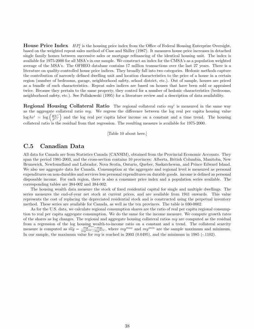
House Price Index HP it is the housing price index from the Office of Federal Housing Enterprize Oversight,

based on the weighted repeat sales method of Case and Shiller (1987). It measures house price increases in detachedsingle family homes between successive sales or mortgage refinancing of the identical housing unit. The index isavailable for 1975-2000 for all MSA’s in our sample. We construct an index for the CMSA’s as a population weightedaverage of the MSA’s. The OFHEO database contains 17 million transactions over the last 27 years. There is aliterature on quality-controlled house price indices. They broadly fall into two categories. Hedonic methods capturethe contribution of narrowly defined dwelling unit and location characteristics to the price of a house in a certainregion (number of bedrooms, garage, neighborhood safety, school district, etc.). Out of sample, houses are pricedas a bundle of such characteristics. Repeat sales indices are based on houses that have been sold or appraisedtwice. Because they pertain to the same property, they control for a number of hedonic characteristics (bedrooms,neighborhood safety, etc.). See Pollakowski (1995) for a literature review and a description of data availability.

Regional Housing Collateral Ratio The regional collateral ratio myi is measured in the same wayas the aggregate collateral ratio my. We regress the difference between the log real per capita housing valuelog hvi = log

(HV i

pa,i

)and the log real per capita labor income on a constant and a time trend. The housing

collateral ratio is the residual from that regression. The resulting measure is available for 1975-2000.


C.5 Canadian Data

All data for Canada are from Statistics Canada (CANSIM), obtained from the Provincial Economic Accounts. Theyspan the period 1981-2003, and the cross-section contains 10 provinces: Alberta, British Columbia, Manitoba, NewBrunswick, Newfoundland and Labrador, Nova Scotia, Ontario, Quebec, Saskatchewan, and Prince Edward Island.We also use aggregate data for Canada. Consumption at the aggregate and regional level is measured as personalexpenditures on non-durables and services less personal expenditures on durable goods. income is defined as personaldisposable income. For each region, there is also a consumer price index and a population series available. Thecorresponding tables are 384-002 and 384-002.

The housing wealth data measure the stock of fixed residential capital for single and multiple dwellings. Theseries measures the end-of-year net stock at current prices, and are available from 1941 onwards. This valuerepresents the cost of replacing the depreciated residential stock and is constructed using the perpetual inventorymethod. These series are available for Canada, as well as the ten provinces. The table is 030-0002.

As for the U.S. data, we calculate regional consumption shares are the ratio of real per capita regional consump-tion to real per capita aggregate consumption. We do the same for the income measure. We compute growth ratesof the shares as log changes. The regional and aggregate housing collateral ratios my are computed as the residualfrom a regression of the log housing wealth-to-income ratio on a constant and a trend. The collateral scarcitymeasure is computed as my = mymax−myt

mymax−mymin , where mymax and mymin are the sample maximum and minimum.In our sample, the maximum value for my is reached in 2003 (0.0495), and the minimum in 1985 (-.1102).

38

Table 1: Income Growth Elasticity of Consumption Shares in Data

Panel A: Specification I Panel B: Specification II

Coll. Measure a1 σa1 R2 b1 σb1 b2 σb2 R2

1 myrw .70 (.05) 6.4 .35 (.03) -.30 (.26) 6.5

2 myfa .75 (.06) 6.9 .36 (.03) -1.74 (.50) 6.8

3 myrw .70 (.03) 4.7 .33 (.02) -.64 (.17) 4.7

4 myfa .78 (.03) 5.0 .37 (.02) -2.12 (.31) 5.0

5 myrw 1.02 (.05) 10.5 .48 (.02) -1.03 (.23) 10.5

6 myfa 1.08 (.05) 10.3 .51 (.03) -1.13 (.30) 10.4

7 myrw .63 (.07) .31 (.04) -.32 (.38)

8 myfa .69 (.08) .32 (.04) -1.75 (.64)

Notes: In panel A we estimate: ∆ log�cit+1

�= ai

0 + a1fmyt+1∆ log�ηi

t+1

�+ νi

t+1. In panel B we estimate: ∆ log�cit+1

�= bi

0 +

b1∆log�ηi

t+1

�+ b2myt+1∆log

�ηi

t+1

�+ νi

t+1. Rows 1-2 are for the period 1952-2002 (1166 observations). Rows 3-4 are identical torows 1-2 but are for the period 1970-2000 (713 observations) in panel A and 1970-2002 (759 observations) in panel B. The measureof regional income is disposable personal income in rows 1-4 and 7-8. Regressions 5-6 use labor income plus transfers, available onlyfor 1970-2000. In each block, the rows use the variables myrw and myfa, estimated for the period 1925-2002. mymax (mymin) isthe sample maximum (minimum) in 1925-2002. The coefficients on the fixed effect, ai

0, are not reported. Estimation is by feasibleGeneralized Least Squares, allowing for both cross-section heteroscedasticity and contemporaneous correlation. Rows 7-8 are the resultsfor the instrumental variable estimation by 3SLS. Instruments are a constant, log(ηi

t+2), log(ηit+3), log(ηi

t+4), ∆ρit+2, ∆ρi

t+3, ∆ρit+4,

log(cit+2), log(ci

t+3), log(cit+4), and myt+2, myt+3, myt+4. The sample is 1952-1998 (1051 observations). All results are for 23 US

metropolitan areas.

39

Table 2: Income Growth Elasticity of Consumption Shares in Model

Panel A Panel B Panel C

β a1 R2 b1 b2 R2 mymin mymax mean(my)

.95 0.323 0.077 0.385 −1.596 0.077 0.026 0.267 .106

.90 0.542 0.074 0.552 −1.498 0.074 0.034 0.284 .106

.85 0.550 0.068 0.553 −1.434 0.068 0.034 0.266 .106

.75 0.584 0.070 0.628 −1.883 0.071 0.042 0.277 .106

Notes: The sample is a model-simulated panel for 1000 years (annual data) and 100 regions with γ = 2, ε = .5 and the AR(1) process forthe non-housing expenditure share in equation (2.5). Each row corresponds to a different value of the time discount factor β. In panel Awe estimate: ∆ log

�cit+1

�= ai

0 + a1fmyt+1∆log�ηi

t+1

�+ νi

t+1. The first and second columns of panel A report the slope coefficient and

the regression’s R2. In panel B we estimate: ∆ log�cit+1

�= bi

0 + b1∆log�ηi

t+1

�+ b2myt+1∆log

�ηi

t+1

�+ νi

t+1. The three last columnsof the table in Panel C report the min, max and mean of the collateral ratio myt over the simulated sample. The mean of my is .10and the mean of fmy is .71.

40

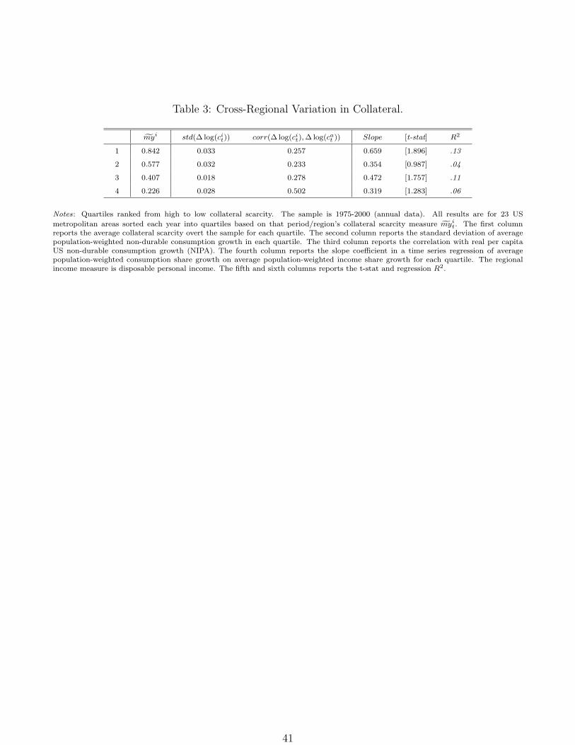
Table 3: Cross-Regional Variation in Collateral.

fmyi std(∆ log(cit)) corr(∆ log(ci

t), ∆log(cat )) Slope [t-stat] R2

1 0.842 0.033 0.257 0.659 [1.896] .13

2 0.577 0.032 0.233 0.354 [0.987] .04

3 0.407 0.018 0.278 0.472 [1.757] .11

4 0.226 0.028 0.502 0.319 [1.283] .06

Notes: Quartiles ranked from high to low collateral scarcity. The sample is 1975-2000 (annual data). All results are for 23 US

metropolitan areas sorted each year into quartiles based on that period/region’s collateral scarcity measure fmyit. The first column

reports the average collateral scarcity overt the sample for each quartile. The second column reports the standard deviation of averagepopulation-weighted non-durable consumption growth in each quartile. The third column reports the correlation with real per capitaUS non-durable consumption growth (NIPA). The fourth column reports the slope coefficient in a time series regression of averagepopulation-weighted consumption share growth on average population-weighted income share growth for each quartile. The regionalincome measure is disposable personal income. The fifth and sixth columns reports the t-stat and regression R2.

41

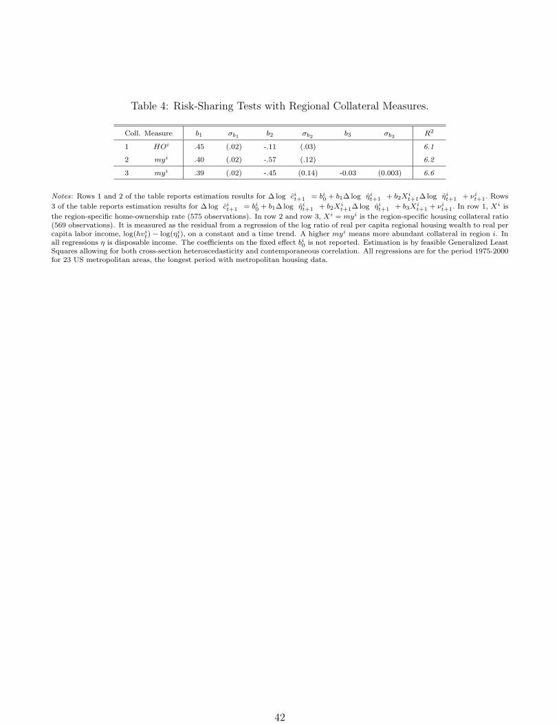
Table 4: Risk-Sharing Tests with Regional Collateral Measures.

Coll. Measure b1 σb1 b2 σb2 b3 σb3 R2

1 HOi .45 (.02) -.11 (.03) 6.1

2 myi .40 (.02) -.57 (.12) 6.2

3 myi .39 (.02) -.45 (0.14) -0.03 (0.003) 6.6

Notes: Rows 1 and 2 of the table reports estimation results for ∆ log�cit+1

�= bi

0 + b1∆log�ηi

t+1

�+ b2Xi

t+1∆log�ηi

t+1

�+ νi

t+1. Rows

3 of the table reports estimation results for ∆ log�cit+1

�= bi

0 + b1∆log�ηi

t+1

�+ b2Xi

t+1∆log�ηi

t+1

�+ b3Xi

t+1 + νit+1. In row 1, Xi is

the region-specific home-ownership rate (575 observations). In row 2 and row 3, Xi = myi is the region-specific housing collateral ratio(569 observations). It is measured as the residual from a regression of the log ratio of real per capita regional housing wealth to real percapita labor income, log(hvi

t)− log(ηit), on a constant and a time trend. A higher myi means more abundant collateral in region i. In

all regressions η is disposable income. The coefficients on the fixed effect bi0 is not reported. Estimation is by feasible Generalized Least

Squares allowing for both cross-section heteroscedasticity and contemporaneous correlation. All regressions are for the period 1975-2000for 23 US metropolitan areas, the longest period with metropolitan housing data.

42

Table 5: Risk-Sharing Tests with Canadian Data.

Panel A: Specification I

Coll. Measure a1 σa1 R2

1 myfa .33 (.03) 36.6

Panel B: Specification II

Coll. Measure b1 σb1 b2 σb2 R2

2 myfa .15 (.02) -2.03 (.41) 37.3

3 myi .18 (.02) -.83 (.28) 34.9

Panel C: Wealth Effect

Coll. Measure b1 σb1 b2 σb2 b3 σb3 R2

4 myi .18 (.02) -.78 (0.29) −0.008 (0.002) 35.1

Notes: In row 1 (panel A) we estimate: ∆ log�cit+1

�= ai

0+a1fmyt+1∆ log�ηi

t+1

�+νi

t+1. In row 2 (panel B) we estimate: ∆ log�cit+1

�=

bi0 + b1∆log

�ηi

t+1

�+ b2myt+1∆log

�ηi

t+1

�+ νi

t+1. Rows 1 and 2 use the aggregate collateral measure for Canada myfa. Row 3 (panel

B) reports estimation results for ∆ log�cit+1

�= bi

0 + b1∆log�ηi

t+1

�+ b2Xi

t+1∆log�ηi

t+1

�+ νi

t+1. Finally, row 4 (panel C) reports

estimation results for ∆ log�cit+1

�= bi

0 + b1∆log�ηi

t+1

�+ b2Xi

t+1∆log�ηi

t+1

�+ b3Xi

t+1 + νit+1. In rows 3 and 4, Xi is the regional

collateral measure myi in Canadian province i. Both the aggregate and regional housing collateral ratios are measured as the residualfrom a regression of the log ratio of real per capita regional housing wealth to real per capita labor income on a constant and a timetrend. The coefficients on the fixed effect, ai

0 or bi0 are not reported. Estimation is by feasible Generalized Least Squares allowing for

both cross-section heteroscedasticity and contemporaneous correlation. All regressions are for the period 1981-2003 for 10 Canadianprovinces. The panel contains 220 observations.

43

Table 6: Population and Composition of Metropolitan Areas.

Anchorage (AK), MSA 261 Miami CMSA 3,897Atlanta (GA), MSA 4,145 Miami, FL 58.1%Baltimore (MD), MSA 2,557 Fort Lauderdale, FL 41.9%Boston CMSA 6,068 Milwaukee CMSA 1,691

Boston, MA-NH 58.6% Milwaukee-Waukesha, WI 88.8%Worcester, MA-CT 8.7% Racine, WI 11.2%Lawrence, MA-NH 6.7% Minneapolis (MN-WI) MSA 2,797Lowell, MA-NH 5.1% New York CMSA 21,134Brockton, MA 4.3% New York, NY 45.5%Portsmouth-Rochester, NH-ME 4.2% Bergen-Passaic, NJ 6.6%Manchester, NH 3.4% Bridgeport, CT 0.5%Nashua, NH 3.3% Dutchess County, NY 1.2%New Bedford, MA 3.2% Danbury, CT 0.4%Fitchburg-Leominster, MA 2.5% Jersey City, NJ 3.0%

Buffalo (NY), MSA 1,169 Middlesex-Somerset-Hunterdon, NJ 5.6%Chicago CMSA 9,176 Monmouth-Ocean, NJ 5.4%

Chicago, IL 90.3% Nassau-Suffolk, NY 13.5%Gary, IN 6.9% Newburgh, NY-PA 1.8%Kenosha, WI 1.6% Newark, NJ 9.9%Kankakee, IL 1.1% New Haven-Meriden, CT 6.2%

Cincinnati CMSA 1,983 Stamford-Norwalk, CT 0.6%Cincinnati, OH-KY-IN 92.6% Trenton, NJ 1.7%Hamilton-Middletown, OH 7.4% Waterbury, CT 0.5%

Cleveland CMSA 2,946 Philadelphia CMSA 6,194Cleveland-Lorain-Elyria, OH 76.4% Philadelphia, PA-NJ 82.4%Akron, OH 23.6% Wilmington, NC 9.5%

Dallas CMSA 5,254 Atlantic-Cape May, NJ 5.7%Dallas, TX 67.4% Vineland-Millville-Bridgeton, NJ 2.3%Fort Worth-Arlington, TX 32.6% Phoenix - Mesa MSA 3,276

Denver CMSA 2,597 Pittsburgh (PA), MSA 2,356Denver, CO 81.7% Portland CMSA 2,273Boulder-Longmont, CO 11.3% Portland-Vancouver, OR-WA 84.7%Greeley, CO 7.0% Salem, OR 15.3%

Detroit CMSA 5,463 Saint Louis (MO-IL), MSA 2,606Detroit, MI 81.4% San Diego (CA), MSA 2,825Ann Arbor, MI 10.6% San Francisco CMSA 7,056Flint, MI 8.0% San Francisco, CA 24.6%

Honolulu (HI), MSA 876 San Jose, CA 23.9%Houston CMSA 4,694 Oakland, CA 34.1%

Houston, TX 89.5% Vallejo-Fairfield-Napa, CA 7.4%Galveston-Texas City, TX 5.3% Santa Cruz-Watsonville, CA 3.6%Brazoria, TX 5.2% Santa Rosa, CA 6.5%

Kansas City (MO-KS), MSA 1,782 Seattle CMSA 3,562Los Angeles CMSA 16,440 Seattle-Bellevue-Everett, WA 67.9%

Los Angeles-Long Beach, CA 58.1% Tacoma, WA 19.8%Orange County, CA 17.4% Bremerton, WA 6.5%Riverside-San Bernardino, CA 20.0% Olympia, WA 5.8%Ventura, CA 4.6% Tampa (FL), MSA 2,404

Washington,DC-MD-VA-WV, PMSA 4,948

Total population numbers (in thousands) are displayed next to the metropolitan areas. For the Consolidated Metropolitan areas(CMSA), the constituent MSA’s are listed and the fraction of their population in the total of the CMSA is shown next to their name.All numbers are from the Regional Economic Information System of the Bureau of Economic Analysis for the year 2000.

44

Table 7: Comparison With Aggregate US data.

Year HH metr. HH NDS NDS to DS DS to EBI EBI to(000) (%) ($) NDC ($) DC ($) DI

1951 17,623 39.4 3,008 1.23 799 1.36 5,959 1.151960 23,080 43.7 3,519 1.22 899 1.26 7,711 1.111970 28,332 44.7 4,688 1.09 1,180 1.05 11,936 1.031980 36,144 44.7 9,683 1.12 2,660 1.24 24,975 1.001990 41,784 44.8 15,418 1.15 5,531 1.37 43,698 0.952000 49,379 47.2 24,741 1.30 11,888 1.90 56,566 0.83

The first column gives the number of households in the metropolitan data set. The second column gives the fraction of US householdsthat are in the metropolitan data set. The third column gives the nondurable retail sales per household (in $) in the metropolitan dataset (NDS). The fourth column gives the ratio of non-durable retail sales per household to non-durable consumption per household inthe NIPA data (NDC). The fifth and sixth column do the same for durable sales and consumption (DS and DC). The seventh andeight column give the effective buying income per household in the metropolitan data set (EBI) and the ratio of the latter to disposableincome per household from NIPA (DI).

45

Table 8: Comparison With Household Data.

MSA Nond.Cons Dur.Cons IncomeWashington, DC (PMSA) 0.926 0.660 0.973Baltimore, MD (PMSA) 0.973 0.791 0.956

Atlanta, GA (MSA) 0.740 0.522 0.944Miami, FL (CMSA) 0.533 0.399 0.922Dallas, TX (CMSA) 0.939 0.839 0.917

Houston, TX (CMSA) 0.936 0.955 0.932Los Angeles, CA (CMSA) 0.836 0.845 0.944

San Francisco, CA (CMSA) 0.921 0.797 0.981San Diego, CA (MSA) 0.838 0.511 0.961Portland, OR (CMSA) 0.989 0.932 0.973Seattle, WA (CMSA) 0.928 0.841 0.935Honolulu, HI (MSA) 0.858 0.409 0.956

Anchorage, AK (MSA) 0.931 0.601 0.847New York, NY (CMSA) 0.952 0.727 0.957

Philadelphia, PA (CMSA) 0.812 0.698 0.932Boston, MA (CMSA) 0.876 0.515 0.799Pittsburgh, PA (MSA) 0.921 0.759 0.846Chicago, IL (CMSA) 0.803 0.601 0.953Detroit, MI (CMSA) 0.960 0.534 0.956

Milwaukee, WI (CMSA) 0.792 0.636 0.949Minneapolis-St, Paul, MN (MSA) 0.940 0.863 0.972

Cleveland, OH (CMSA) 0.881 0.878 0.956Cincinnati, OH (CMSA) 0.898 0.864 0.974St. Louis, MO (MSA) 0.881 0.815 0.945

Kansas City, MO-KS (MSA) 0.958 0.708 0.961Average 0.881 0.708 0.938

Correlation of household non-durable consumption, durable consumption and income data, aggregated by the CEX for metropolitanareas and the metropolitan area non-durable and durable retail sales and disposable income data from S&MM.

46

Table 9: Comparison With Regional Income DataSouth and West Coeff. Northeast and Midwest Corr.

Washington, DC (PMSA) 0.79 New York, NY (CMSA) 0.84Baltimore, MD (PMSA) 0.42 Philadelphia, PA (CMSA) 0.82

Atlanta, GA (MSA) 0.73 Boston, MA (CMSA) 0.73Miami, FL (CMSA) -0.18 Pittsburgh, PA (MSA) 0.57Dallas, TX (CMSA) 0.63 Buffalo, NY (MSA) 0.77

Houston, TX (CMSA) 0.86 Chicago, IL (CMSA) 0.76Los Angeles, CA (CMSA) 0.85 Detroit, MI (CMSA) 0.74

San Francisco, CA (CMSA) 0.65 Milwaukee, WI (CMSA) 0.12San Diego, CA (MSA) 0.75 Minneapolis-St, Paul, MN (MSA) 0.70Portland, OR (CMSA) 0.57 Cleveland, OH (CMSA) 0.90Seattle, WA (CMSA) 0.60 Cincinnati, OH (CMSA) -0.23Honolulu, HI (MSA) 0.84 St. Louis, MO (MSA) 0.54

Anchorage, AK (MSA) 0.80 Kansas City, MO-KS (MSA) 0.57Phoenix, AZ (MSA) 0.83Denver, CO (CMSA) 0.67 Average 0.64

Correlation of regional disposable income from S&MM and labor income plus Transfers from REIS.

47

Table 10: Median Home Value and Home-Ownership Rate.

MSA V80 V00 HO80 HO00

Washington, DC (PMSA) 79.9 178.9 54.3 64.0Baltimore, MD (PMSA) 51.4 134.9 60.0 66.9Atlanta, GA (MSA) 47.7 135.3 61.4 66.4Miami, FL (CMSA) 57.0 126.1 61.5 63.2Dallas-Fort Worth, TX (CMSA) 45.6 100.0 64.7 60.4Houston, TX (CMSA) 52.8 89.7 59.1 60.7Tampa, FL (MSA) 39.9 93.8 71.7 70.8

San Francisco, CA (CMSA) 98.4 353.5 55.8 57.8Los Angeles, CA (CMSA) 87.6 203.3 53.8 54.8San Diego, CA (MSA) 90.0 227.2 55.1 55.4Portland, OR (CMSA) 60.8 165.4 63.2 63.0Seattle, WA (CMSA) 66.0 195.4 63.8 62.9Honolulu, HI (MSA) 129.5 309.0 49.9 54.6Anchorage, AK (MSA) 89.2 160.7 56.6 60.1Denver, CO (CMSA) 69.1 179.5 63.0 66.4Phoenix, AZ (MSA) 59.2 127.9 68.7 68.0

New York, NY (CMSA) 62.5 203.1 44.2 53.0Philadelphia, PA (CMSA) 42.2 122.3 67.7 69.9Boston, MA (CMSA) 52.0 203.0 54.8 60.6Pittsburgh, PA (MSA) 42.7 68.1 69.0 71.3Buffalo, NY (MSA) 39.7 89.1 63.7 66.2

Chicago, IL (CMSA) 62.8 159.0 58.5 65.2Detroit, MI (CMSA) 43.5 132.6 70.2 72.2Milwaukee, WI (CMSA) 59.2 131.9 61.1 62.1Minneapolis-St, Paul, MN (MSA) 62.3 141.2 67.2 72.4Cleveland, OH (CMSA) 52.1 117.9 66.6 68.8Cincinnati, OH (CMSA) 47.9 116.5 63.8 67.1St. Louis, MO (MSA) 41.8 99.4 68.2 71.4Kansas City, MO-KS (MSA) 43.5 104.7 66.4 67.9Tampa, FL (MSA) 59.9 85.2 73.0 71.0

The table shows median home values for 1980 and 2000 (in thousands of nominal dollars) and the home ownership rate for 1980 and2000. All data are from the US Bureau of the Census, Decennial Survey 1980 and 2000

48

1952 1962 1972 1982 1992 20020.2

0.3

0.4

0.5

0.6

0.7

Col

late

ral S

carc

ity

0.8

1

1.2

1.4

1.6

1.8Std(cons)/std(y)

Year

Con

sum

ptio

n−to

−In

com

e D

ispe

rsio

n

Figure 1: Housing Collateral Scarcity and Consumption/Income Dispersion in Data.This figure plots the ratio of regional consumption-to-income dispersion (dashed line, plotted against the right axis). Both consumptionand income are measured in deviation from the cross-regional mean. The solid line is our collateral scarcity measure, plotted againstthe left axis. The sample consists of annual data from 1952 until 2002 for 23 US Metropolitan Statistical Areas. The data are discussedin section 3.1.

49

0 50 100 150 200 250 300 350 400 450 5000.5

0.6

0.7

0.8

0.9

1

1.1

1.2

1.3

1.4

1.5

Simulation Periods

Con

sum

ptio

n−to

−Inc

ome

Dis

pers

ion

0 50 100 150 200 250 300 350 400 450 5000.5

0.55

0.6

0.65

0.7

0.75

0.8

0.85

0.9

0.95

1

colla

tera

l sca

rcity

Figure 2: Housing Collateral Scarcity and Consumption/Income Dispersion in Model.The figure plots a simulated time path for T = 500 of the collateral scarcity measure fmy (solid line, measured against the right axis)against the ratio of regional consumption dispersion to regional income dispersion (dashed line, measured against the left axis). Theparameters are γ = 2, ε = .5, β = .95. The average collateral ratio is 10 percent.

50

0.4 0.5 0.6 0.7 0.8 0.9 10.7

0.8

0.9

1

1.1

1.2

1.3

1.4

Collateral Scarcity

Cons

umpt

ion−

to−I

ncom

e Di

sper

sion

0.4 0.5 0.6 0.7 0.8 0.9 10.2

0.25

0.3

0.35

0.4

0.45

0.5

Collateral Scarcity

Cons

umpt

ion−

to−I

ncom

e Di

sper

sion

Figure 3: The Quantity Anomaly at the Regional Level.Scatter diagram of collateral and consumption-to-income dispersion ratios. The upper panel is for regions. The lower panel is forhouseholds. The figure plots, for a simulated time path (T = 2, 500), the collateral scarcity measure gmyt (horizontal axis) against theratio of regional consumption dispersion to regional income dispersion (vertical axis, upper panel), and household consumption-to-incomedispersion (vertical axis, lower panel). The parameters are γ = 2, ε = .5, β = .95. The average collateral ratio is 10 percent.

51

how much does household collateral constrain regional risk

Documents