How General is Human Capital? A Task-Based Approach

Christina Gathmann

Stanford University

Uta Schönberg

University College London

This Draft: August 2008

Abstract

This paper studies how portable skill accumulated in the labor market are. Using rich data ontasks performed in occupations, we propose the concept of task-speci�c human capital to measurethe transferability of skills empirically. Our results on occupational mobility and wages show thatlabor market skills are more portable than previously considered. We �nd that individuals move tooccupations with similar task requirements and that the distance of moves declines with time in thelabor market. We also show that task-speci�c human capital is an important source of individual wagegrowth, in particular for university graduates. For them, at least 40 percent of overall wage growth overa ten year period can be attributed to task-speci�c human capital. For the low- and medium-skilled,task-speci�c human capital accounts for at least 35 and 25 percent of overall wage growth respectively.

Correspondence: Christina Gathmann, CHP/PCOR, Stanford University; Uta Schönberg, Department ofEconomics, University College London. We thank Katherine Abraham, Min Ahn, Mark Bils, Nick Bloom, SusanDynarski, Anders Frederiksen, Donna Ginther, Galina Hale, Bob Hall, Henning Hillmann, Pete Klenow, EdLazear, Petra Moser, John Pencavel, Luigi Pistaferri, Richard Rogerson, Michele Tertilt, participants at theSociety of Labor Economists Meeting, the Society of Economic Dynamics Meeting, the World Congress of theEconometric Society and numerous institutions for helpful comments and suggestions. All remaining errors areour own.

1 Introduction

Human capital theory (Becker, 1964; Mincer, 1974) and job search models (e.g. Jovanovic, 1979a;

1979b) are central building blocks for economic models of the labor market. Both are widely used to

study job mobility behavior, wage determination and their aggregate implications for wage inequality,

unemployment and economic growth.

A crucial decision in these models is how to characterize labor market skills. Human capital and job

search theories typically distinguish between general skills like education and experience and speci�c

skills, i.e. skills that are not portable across jobs. Recent contributions have focused on the importance

of speci�c skills to explain phenomena like the growth di¤erences between continental Europe and the

United States (e.g. Wasmer, 2004), the rise of unemployment in continental Europe (e.g. Ljungqvist and

Sargent, 2005) and the surge in wage inequality over the past decades (e.g. Violante, 2002; Kambourov

and Manovskii, 2007a). The basic idea is that job reallocation, job displacement and unemployment

are more costly for the individual worker and the economy if skills are not transferable across jobs.

However, we know little about how portable skills accumulated in the labor market actually are. In

this article, we propose the concept of �task-human capital�to measure the speci�city of labor market

skills empirically.1 We then use this concept to show that human capital is more portable than previously

considered.

The basic idea of our approach is straightforward. Suppose there are two types of tasks performed

in the labor market, for example analytical and manual tasks. Both tasks are general in the sense that

they are productive in many occupations. Occupations combine these two tasks in di¤erent ways. For

example, one occupation (e.g. accounting) relies heavily on analytical tasks, a second one (e.g. bakers)

more on manual tasks, and a third combines the two in equal proportion (e.g. musicians).

Skills accumulated in an occupation are then �speci�c�because they are only productive in occu-

pations which place a similar value on combinations of tasks (see also Lazear, 2003). This type of

1Our concept of task human capital is closely related to the ideas proposed in Gibbons and Waldman (2004; 2006).However, they apply the idea to internal promotions and job design while we use it to study occupational mobility andwage growth.

2

task-speci�c human capital di¤ers from general skills because it is valuable only in occupations that

require skills similar to the current one. It di¤ers from occupation-speci�c skills in that it does not fully

depreciate if an individual leaves his occupation. Compare, for instance, a carpenter who decides to

become a cabinet maker with a carpenter who decides to become a baker. In our approach, the former

can transfer more skills to his new occupation than the latter.

Our data is uniquely suited to analyze the transferability of skills empirically. It combines infor-

mation on tasks performed in di¤erent occupations with a high-quality panel on complete job histories

and wages. The �rst data is a large panel that follows individual labor market careers from 1975 to

2001. The data, derived from a two percent sample of all social security records in Germany, provides

a complete picture of job mobility and wages for more than a 100,000 workers. It has several distinct

advantages over the data used in the previous literature on occupational mobility. First, the admin-

istrative nature of our data ensures that there is little measurement error in wages and occupational

coding. Both are serious problems in data sets like the PSID or NLSY used previously. Furthermore,

we have much larger samples available than in typical household surveys.

The third advantage of our data is that we can measure what tasks are performed in di¤erent

occupations. This information comes from a large survey of 30,000 employees at four separate points

in time. Exploiting the variation in task usage across occupations and time, we construct a continuous

measure of skill distance between occupations. Based on the task data, the skill requirements of a baker

and a cook are very similar. In contrast, switching from a banker to an unskilled construction worker

would be the most distant move observable in our data. We then use this skill distance measure together

with the panel on job mobility to construct an individual�s task-human capital.

We �nd that individuals are much more likely to move to similar occupations than suggested by

search and turnover models in which the source occupation has no impact on the choice of future

occupations. The distance of actual moves like the propensity to switch occupations declines sharply

with labor market experience. These results are consistent with the idea that task-speci�c human capital

is an important determinant of occupational mobility.

3

If human capital is largely task-speci�c and therefore transferable to similar occupations, this should

also be re�ected in individuals�wages. Our framework can explain why tenure in the pre-displacement

job has been found to have a positive e¤ect on the post-displacement wage, especially in high-skilled

occupations (Kletzer, 1989). We also show that wages and tenure in the last occupation have a stronger

e¤ect on wages in the new occupation if the two occupations require similar skills.

We then show that task-speci�c human capital is an important determinant of individual wage

growth compared to other general and speci�c skills, using a control function approach. Occupation-

speci�c skills and general experience become less important for wage growth once we include task

speci�c human capital. For university graduates, at least 40 percent of wage growth due to human

capital accumulation can be attributed to task-speci�c skills. For the medium-skilled (low-skilled), at

least 25 (35) percent of individual wage growth is due to task-speci�c human capital.

Our results have important implications for the costs of job reallocation and hence welfare in an

economy. We illustrate this by calculating the costs of job displacement for the individual worker.

Workers who are able to �nd employment in occupations with similar skill requirements lose 12 percent

of their wages; wage losses are almost three times as high if they have to move to very distant occupations

instead. Hence, reallocation costs in an economy will depend crucially on the thickness of the labor

market.

The article makes several contributions to the literature. First, we introduce a novel way to de�ne

how occupations are related to each other in terms of their skill requirements. In particular, we use data

on actual tasks performed in occupations to characterize the distance between occupations along a con-

tinuous scale. Previous empirical papers on the transferability of skills across occupations (Shaw, 1984;

1987) have used the frequency of occupational switches to de�ne similar occupations (i.e. occupations

that often exchange workers are assumed to have similar skill requirements).

Second, using our distance measure, we document novel patterns in mobility that are consistent

with our view that speci�c labor market skills are more portable than previously considered. A key

implication of our framework, which we con�rm with our data, is that the source occupation has a strong

4

in�uence on the choice of one�s future occupation. The literature on �rm and occupational mobility in

contrast focuses on the determinants of switching �rms (Flinn, 1986; Topel and Ward, 1992) or both

�rms and occupations (McCall, 1990; Miller, 1984; Neal, 1998; Pavan, 2005), but has not studied the

type and direction of a move.2

Our third contribution is to quantify the contribution of task-speci�c human capital to individual

wage growth and compare it to other forms of human capital like experience and occupational tenure.

While a large number of studies have estimated the contribution of �rm-speci�c human capital to

individual wage growth (Abraham and Farber, 1987; Altonji and Shakotko, 1987; Altonji and Williams,

2005; Topel, 1991; Kletzer, 1989)3, recent evidence suggests that speci�c skills might be more tied to an

occupation than to a particular �rm (Gibbons et al., 2006; Kambourov and Manovskii, 2007b; Parent,

2000; Neal, 1999). We show in contrast that speci�c human capital is not fully lost if an individual

leaves an occupation. Poletaev and Robinson (2008) report a similar result using information from the

Dictionary of Occupational Titles (DOT). In addition, we are able to quantify the role of task-speci�c

skills for wage growth over the life-cycle.

Finally, our paper provides the �rst attempt to integrate the recent literature using task data (Autor

et al., 2003; Spitz-Öner, 2006; Borghans et al., 2006) with human capital models of the labor market.4

Our paper employs data on tasks to propose a new measure of the speci�city of skills. In contrast to the

literature on task usage, we abstract from which particular task (analytical, manual etc.) matters for

mobility and wages. Instead, we explore the implications of task-speci�c human capital for occupational

mobility, the direction of the occupational move, and the transferability of human capital.

The paper proceeds as follows. The next section outlines our concept of task human capital and how

it relates to the previous literature on labor market skills. Section 3 introduces the two data sources

2 In a paper complementary to ours, Malamud (2005) analyzes how the type of university education a¤ects occupationalchoice and mobility.

3See Farber (1999) for a comprehensive survey of this literature.4Autor et al. (2003) for the United States and Spitz-Öner (2006) for West Germany study how technological change

has a¤ected the usage of tasks, while Borghans et al. (2006) show how the increased importance of interactive skills hasimproved the labor market outcomes of under-represented groups. Similarly, Ingram and Neumann (2006) argue thatchanges in the returns to tasks performed on the job are an important determinant of wage di¤erentials across educationgroups.

5

and explains how we measure the distance between occupations in terms of their task requirements.

Descriptive evidence on the similarity of occupational moves and its implications for wages across

occupations are presented in Section 4. Section 5 quanti�es the importance of task-speci�c human

capital for individual wage growth and calculates wage costs of job displacement. Finally, Section 6

concludes.

2 Conceptual Framework

2.1 Task-Speci�c Human Capital

This section de�nes how occupations are related to each other and introduces our concept of task-

speci�c human capital. Suppose that output in an occupation is produced by combining multiple tasks,

for example negotiating, teaching or managing personnel. These tasks are general in the sense that

they are productive in di¤erent occupations. Occupations di¤er in which tasks they require and in the

relative importance of each task for production. An individual�s productivity is then �speci�c�to that

occupation because occupations place di¤erent values on combinations of skills.

More speci�cally, consider the case of two tasks, denoted by j = A;M . We think of them as

manual and analytical tasks. Workers are endowed with a productivity in each task, which we denote

by T jit; j = A;M: Occupations combine the two tasks in di¤erent ways. For example, one occupation

might rely heavily on analytical tasks, a second more on manual tasks, and a third combines the two

in equal proportion. Let �o (0 � �o � 1) be the relative weight on the analytical task, and (1� �o) be

the relative weight on the manual task. We specify worker i�s productivity (measured in log units) in

occupation o as

lnSit = �oTAit + (1� �o)TMit :

For example, if in an occupation analytical tasks are more important than manual tasks, �o > 0:5: In

another occupation, only the manual task might be performed, so �o = 0: By restricting the weights on

the tasks to sum to one, we focus on the relative importance of each task, not on the task intensity of

6

an occupation. We impose this restriction for illustrative purposes only. None of our empirical results

below require this restriction.

In this approach, we can de�ne the relation between occupations in a straightforward way. Two

occupations o and o0 are similar if they employ analytical and manual tasks in similar proportions, i.e. �o

is close to �o0 . We can then measure the distance between the two occupations as the absolute di¤erence

between the weight given to the analytic task in each occupation, i.e. j�o � �o0 j. The maximum distance

of one is between an occupation that fully specializes in the analytical task (�o = 1) and the one that

fully specializes in the manual task (�o = 0).

We further assume that log-productivity can be decomposed into a time-varying component that

captures human capital accumulation, Xiot o; and a time-invariant component that captures the quality

of the occupational match, �oTAi + (1� �o)TMi :5

lnSiot = oXiot| {z } + �oT

Ai + (1� �o)TMi| {z }

Human Capital Match Quality

We now describe each component in turn.

Human Capital Accumulation With time in the labor market, individuals become more pro-

ductive in each task through learning-by-doing. In particular, we assume that Xiot contains three types

of human capital: general human capital (Expit), purely occupation-speci�c human capital (OTit), and

what we call task-speci�c human capital (TTit). The vector o = [ 1o 2o 3o] denotes the returns to

the three types of human capital, which vary across occupations. This speci�cation takes seriously the

existing empirical evidence that returns to labor market skills di¤er across occupations (for example,

Gibbons et al, 2005; Heckman and Sedlacek, 1985).

General human capital is valuable in all occupations, while occupation-speci�c human capital is

fully lost once a worker leaves the occupation. Task-speci�c human capital in contrast is transferable to

5For simplifaction, we do not incorporate the search for a �rm match here. We discuss the implications of matchingacross �rms in Section 5.4 below.

7

occupations with similar skill requirements. More speci�cally, we assume that the transferability of skills

between the source and destination occupation depends on the distance between the two occupations:

Workers can transfer a fraction 1�j�o � �o0 j of their human capital if they switch from occupation o to

o0: For example, if workers move from an occupation that fully specializes in the analytical task (�o = 1)

to an occupation that fully specializes in the manual task (�o0 = 0), none of the acquired skills can be

transferred. If, in contrast, workers move from an occupation that mostly uses the analytical task (e.g.

�o = 0:75) to an occupation that employs both tasks in equal proportions (e.g. �o0 = 0:5), they are

able to transfer 75 percent of their acquired skills. Hence, task-speci�c human capital is neither fully

general nor purely speci�c, but partially transferable across occupations.

Using these assumptions, we can collapse the accumulation of skills in multiple tasks into a one-

dimensional observable measure of task-speci�c human capital, TTit: We calculate task human capital

from occupation tenure in all previous occupations, inversely weighted by the distance between the

current and previous occupations. We therefore abstract from estimating human capital accumulation

separately in each task, and instead focus on the portability of skills from one occupation to another.

One advantage of this approach is that we can compare the importance of task-speci�c human capital

to other, more standard measures of human capital like experience or occupational tenure.

Match Quality The occupation-speci�c match component is speci�ed as a weighted average of

the individual�s productivity in each task, �oTAi + (1 � �o)TMi : Hence, match qualities are correlated

across occupations in our speci�cation if the two occupations rely on similar tasks. Existing mod-

els of occupational choice (for example, Neal (1999) and Pavan (2005)) in contrast assume that the

occupational match is uncorrelated across occupations.

8

2.2 Wage Determination and Occupational Mobility

Wages in occupation o and time t are equal to worker i�s productivity, Siot; multiplied with the

occupation-speci�c skill price, Po; i.e. wiot = PoSiot: Hence, log wages satisfy:

lnwiot = po + lnSiot + "iot = po + oXiot + �oTAi + (1� �o)TMi + "iot

=po + 1oExpit + 2oOTiot + 3oTTit| {z }+ �oT

Ai + (1� �o)TMi + "iot| {z }

observed unobserved

; (1)

where po = lnPo:We have added an iid error term "iot is assumed to be uncorrelated with the regressors

and re�ects for instance measurement error in wages. We observe general (Expit), occupation-speci�c

(OTiot), and task-speci�c skills (TTit):We do not observe the quality of the match, �oTAi +(1��o)TMi :

Since the concept of task-speci�c human capital is novel, we next clarify the interpretation of the return

to task-speci�c human capital, 2o: Consider a worker who has worked for his occupation o for one

year. Suppose he is exogenously displaced from his occupation and then randomly assigned to a new

occupation. A worker who moves to the most similar occupation loses 2o (i.e. the purely occupation-

speci�c skills). In contrast, a worker who moves to the most distant occupation loses 2o + 3o; while a

worker who moves to an occupation where he can transfer �fty percent of his skills loses 2o + 0:5 3o:

Of course, workers are not randomly allocated into occupations. We assume that workers search

over occupations to maximize earnings.6 The decision to switch occupations is determined by three

factors: the potential loss in occupation- and task-speci�c human capital (OTiot; TTit), the task match

(�oTAi + (1� �o)TMi ) and the occupation-speci�c returns to human capital ( 1o, 2o; 3o and po).

If returns to skills are the same across occupations, workers would switch occupations only if the gain

in match quality compensates for the loss in occupation- and task-speci�c human capital. This decision

rule is the same irrespective of whether the search process is completely undirected or partially directed.

In the case of undirected search, workers would search for the best match across all occupations regardless

6For example, Fitzenberger and Kunze (2006) and Fitzenberger and Spitz-Öner (2004) argue that search is the mostimportant source of occupational switches in Germany.

9

of the worker�s true productivity in each task. In the case of partially directed search, workers would

only apply to occupations that promise a better match. Occupational mobility results either because

workers are at labor market entry not fully informed about which occupation provides the best match

at labor market entry, or there is a rationing of jobs in the worker�s most preferred occupation.

If, in contrast, the returns to human capital accumulation in the prospective occupation exceed those

in the current occupation, workers may voluntarily switch occupations even if they lose speci�c human

capital and are worse matched in the new occupation. This may occur because the new occupation

promises higher wage growth in the future than the old one. This result again holds in the case of

random or partially directed search.

Our framework produces a number of novel empirical implications. It implies that, everything else

equal, workers are more likely to move to occupations in which they can perform similar tasks as in their

previous occupation. The reason is that task-speci�c human capital is more valuable in similar than

in distant occupations. We also expect that distant moves occur early, rather than late, in the labor

market career for two reasons. First, the accumulation of task-speci�c human capital makes distant

occupational switches increasingly costly. Second, with time in the labor market, workers gradually

locate better and better occupational matches. It therefore becomes less and less likely that they accept

o¤ers from very distant occupations. Since both the transferability of task-speci�c human capital and

the correlation of match qualities across occupations declines in the occupational distance, we also

expect that wages at the source occupation are a better predictor for wages at the target occupation if

the two occupations require similar tasks.

2.3 Comparison with Alternative Approaches

Our setup is closely related to the Roy model of occupational sorting (Roy, 1951; Heckman and Sed-

lacek, 1985). Just like in the Roy model, individuals in our framework sort themselves into occupations

according to comparative advantage. While the original Roy model allows skills to be arbitrarily corre-

lated across occupations, we impose a linear factor structure with two factors (�oTAit +(1��o)TMit ). This

10

restriction allows us to de�ne how similar occupations are in their skill requirements in a straightforward

way.

Our framework is also related to search and matching models of the labor market (Jovanovic, 1979a;

1979b). As in search or matching models, we include a match component that (partially) determines

mobility decisions. In contrast to existing search and matching models however, our setup incorporates

that speci�c skills are partially transferable and match qualities correlated across occupations. These

extensions provide new insights into the direction of occupational mobility and allow us to quantify the

importance of task-speci�c human capital for individual wage growth relative to other forms of human

capital.

In a recent paper, Lazear (2003) also sets up a model in which �rms use general skills in di¤erent

combinations with �rm-speci�c weights attached to them. In this model, workers are exogenously

assigned to a �rm (in our application: occupation) and then choose how much to invest in each skill. Our

- in our opinion more intuitive - approach assumes instead that workers are endowed with a productivity

in each task, and then choose the occupation. Furthermore, unlike Lazear (2003), our empirical analysis

focus on the transferability of skills across occupations and its implications for occupational mobility

and individual wage growth.

3 Data Sources and Descriptive Evidence

To study the transferability of skills empirically, we combine two di¤erent data sources from Germany.

Further details on the de�nition of variables and sample construction can be found in Appendix A.

3.1 Data on Tasks Performed in Occupations

Our �rst data set contains detailed information on tasks performed in occupations, which we use to

characterize how similar occupations are in their skill requirements. The data come from the repeated

cross-section German Quali�cation and Career Survey, which is conducted jointly by the Federal Insti-

tute for Vocational Education and Training (BIBB) and the Institute for Employment (IAB) to track

11

skill requirements of occupations. The survey, previously used for example by DiNardo and Pischke

(1997) and Borghans et al. (2006), is available for four di¤erent years: 1979, 1985, 1991/92 and 1998/99.

Each wave contains information from 30,000 employees between the ages of 16 and 65. In what follows,

we restrict our analysis to men since men and women di¤er signi�cantly in their work attachments and

occupational choices.

In the survey, individuals are asked whether they perform any of nineteen di¤erent tasks in their

job. Tasks vary from repairing and cleaning to buying and selling, teaching, and planning. For each

respondent, we know whether he performs a certain task in his job and whether this is his main activity.

Table 1 lists the fraction of workers performing each of the nineteen di¤erent tasks. Following Autor

et al. (2003) and Spitz-Öner (2006), we combine the 19 tasks into three aggregate groups: analytical

tasks, manual tasks and interactive tasks. On average, 55 percent report performing analytic tasks, 72

percent manual tasks, and 49 percent interactive tasks. The picture for the main task used is similar:

32 percent report analytical tasks, 57 percent manual tasks and 28 percent interactive tasks as their

main activity on the job.

The last two columns in table 1 show the distribution of tasks performed on the job for two popular

occupations: teacher and baker. According to our task data, a teacher primarily performs interac-

tive tasks (95.3 percent) with teaching and training others being by far the most important one (91.4

percent). Two other important tasks are correcting texts or data (39.6 percent) and organizing, coor-

dinating and managing personnel (39.4 percent). A baker in contrast is a primarily manual occupation

(96.4 percent) with manufacturing, producing, installing as the most important task (87.9 percent) fol-

lowed by teaching and training others (34.3 percent) as well as organizing, coordinating and managing

personnel (29.9 percent).

To see how task usage varies across the 64 occupations contained in our data, table A1 lists the

fraction of workers performing manual, analytical, and interactive tasks for all 64 occupations. The table

shows that there is a lot of variation in task usage across occupations. For example, while the average

use of analytical tasks is 56.3 percent, the mean varies from 16.7 percent as an unskilled construction

12

worker to 92.4 percent for an accountant. We found little evidence that tasks performed in the same

occupation vary across industries, which suggest that industries matter less for measuring human capital

once we control for the skill set of an occupation, and justi�es our focus on occupations.

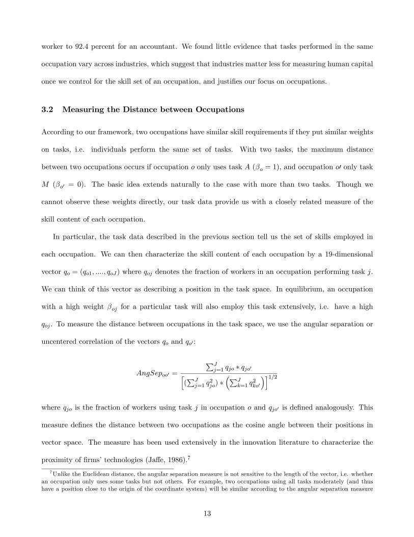
3.2 Measuring the Distance between Occupations

According to our framework, two occupations have similar skill requirements if they put similar weights

on tasks, i.e. individuals perform the same set of tasks. With two tasks, the maximum distance

between two occupations occurs if occupation o only uses task A (�o = 1), and occupation o0 only task

M (�o0 = 0). The basic idea extends naturally to the case with more than two tasks. Though we

cannot observe these weights directly, our task data provide us with a closely related measure of the

skill content of each occupation.

In particular, the task data described in the previous section tell us the set of skills employed in

each occupation. We can then characterize the skill content of each occupation by a 19-dimensional

vector qo = (qo1; ::::; qoJ) where qoj denotes the fraction of workers in an occupation performing task j.

We can think of this vector as describing a position in the task space. In equilibrium, an occupation

with a high weight �oj for a particular task will also employ this task extensively, i.e. have a high

qoj . To measure the distance between occupations in the task space, we use the angular separation or

uncentered correlation of the vectors qo and qo0 :

AngSepoo0 =

PJj=1 qjo � qjo0h

(PJj=1 q

2jo) �

�PJk=1 q

2ko0

�i1=2where qjo is the fraction of workers using task j in occupation o and qjo0 is de�ned analogously. This

measure de�nes the distance between two occupations as the cosine angle between their positions in

vector space. The measure has been used extensively in the innovation literature to characterize the

proximity of �rms�technologies (Ja¤e, 1986).7

7Unlike the Euclidean distance, the angular separation measure is not sensitive to the length of the vector, i.e. whetheran occupation only uses some tasks but not others. For example, two occupations using all tasks moderately (and thushave a position close to the origin of the coordinate system) will be similar according to the angular separation measure

13

We use a slightly modi�ed version of the above, namely Disoo0 = 1 � AngSepoo0 as our distance

measure. The measure varies between zero and one. It is zero for occupations that use identical skill

sets and unity if two occupations use completely di¤erent skills sets. The measure will be closer to zero

the more two occupations overlap in their skill requirements. To account for changes in task usage over

time, we calculated the distance measures separately for each wave. For the years 1975-1982, we use

the measures from the 1979 cross-section, for 1983-1988 the task measures from the 1985 wave; for the

years 1989-1994, we use the measures based on the 1991/2 wave; and the 1997/8 wave for the years

1995-2001. Our results are robust to assigning di¤erent time windows to the measures.8

The mean distance between occupations in our data is 0.24 with a standard deviation of 0.22 (see

Table 2). The most similar occupational move is between paper and pulp processing and a printer

or typesetter with a distance of 0.002. The most distant move is between a banker and an unskilled

construction worker. Table 2 also shows at the bottom the distance measure for the three most common

occupational switches separately by education group. The most popular move for low-skilled worker is

between a truck driver and a warehouse keeper, while for the high skilled, it is between an engineering

occupation and a chemist or physicist.9

3.3 The German Employee Panel

Our second data set is a two percent sample of administrative social security records in Germany from

1975 to 2001 with complete job histories and wage information for more than 100,000 employees. The

data has at least three advantages over household surveys commonly used in the literature to study

mobility in the United States. First, its administrative nature ensures that we observe the exact date

of a job change and the wage associated with each job. Second, occupational titles are consistent across

even if their task vectors are orthogonal, and therefore distant according to the Euclidean distance measure. If all vectorshave the same length (i.e. if all tasks are used by at least some workers in all occupations), our measure is proportional tothe Euclidean distance measure.

8While there have been changes over time in the distance measures, they are with 0.7 highly correlated.9Our distance measure treats all tasks symmetrically. It may, however, be argued that some tasks are more similar

than others. For instance, the task �equipping machines�may be more similar to �repairing�than to �teaching�. In orderto account for this, we also de�ned the angular separation measure using information on the 3 aggregate task groups(analytical, manual and interactive tasks). The results based on this alternative distance measures are qualitatively verysimilar to the ones reported in the paper.

14

�rms as they form the basis for wage bargaining between unions and employers. Finally, measurement

error in earnings and occupational titles are much less of a problem than in typical survey data as

misreporting is subject to severe penalties.

The data is representative of all individuals covered by the social security system, roughly 80 percent

of the German workforce. It excludes the self-employed, civil servants, and individuals currently doing

their compulsory military service. As in many administrative data sets, our data is right-censored at

the highest level of earnings that are subject to social security contributions. Top-coding is negligible

for unskilled workers and those with an apprenticeship, but reaches almost 25 percent for university

graduates. For the high-skilled, we use tobit or semiparametric methods to account for censoring.

Since the level and structure of wages di¤ers substantially between East and West Germany, we drop

from our sample all workers who were ever employed in East Germany. We also drop all those working

in agriculture. In addition, we restrict the sample to men who entered the labor market in or after 1975.

This allows us to construct precise measures of actual experience, �rm, task, and occupation tenure

from labor market entry onwards. Labor market experience and our tenure variables are all measured

in years and exclude periods of unemployment and apprenticeship training.

Since the concept is novel, we now explain how we calculate our measure of task human capital.

Each individual starts with zero task tenure at the beginning of his career. Task tenure increases by the

duration of the spell if a worker remains in the same occupation. If he switches occupations, we calculate

task tenure in the new occupation as the weighted sum of time spent in all previous occupations where

the weights are the distance between the current and all past occupations.10

As an example, consider a person who starts out in occupation A, then switches to occupation

B after one year, and switches to occupation C again after one year. Suppose the distance between

occupation A and B is 0.5, between occupation A and C 0.2 and 0.8 between occupation B and C.

Before moving to occupation B, he has accumulated 1 unit of task tenure. Since he can only transfer 50

10 In principle, our separation measure takes values between 0 and 1. However, the maximum distance observed in ourdata (across all occupation pairs) is 0.93. In our calculation, we assume that a worker cannot transfer any skills if he makesthe most distant occupation switch, and de�ne the relative distance between two occupations A and B as the di¤erencebetween the maximum distance in our data and the distance between occupations A and B, divided by the maximumdistance. Our results do not change if we use the actual distance instead of this relative distance measure.

15

percent of his task human capital to occupation B, his task tenure declines to 0.5. After working one

year in occupation B, he accumulates another unit of task human capital, so task tenure increases to

1.5 (0:5 � 1 + 1). Switching to occupation C after the second year, the worker can transfer 20 percent

of his task human capital he accumulated in occupation A in the �rst period and 80 percent of the

human capital accumulated in occupation B in the second period. His task tenure variables is thus 1 =

0:2 � 1 + 0:8 � 1.

Table 3 reports summary statistics for the main variables. In our sample, about 16 percent are

low-skilled workers with no vocational degree. The largest fraction (68.3 percent) are medium-skilled

workers with a vocational degree (apprenticeship). The remaining 15.4 percent are high-skilled workers

with a tertiary degree from a technical college or university. Wages are measured per day and de�ated

to 1995 German Marks. Mean task tenure in our sample is between 4.6 years for the low-skilled and

4.8 years for the medium-skilled. Total labor market experience is on average a year higher (since the

general skills captured by time spent in the labor market do not depreciate) and about one year lower

for occupation tenure (since this measure assumes that these skills fully depreciate with an occupational

switch).

Occupational mobility is important in our sample: 19 percent of the low-skilled switch occupations

each year and with 11 percent somewhat lower for the high skilled. To see how occupational mobility

varies over the career, �gure 1 plots quarterly mobility rates over the �rst ten years in the labor market,

separately by education group. Occupational mobility rates are very high in the �rst year (particularly

in the �rst quarter) of a career, and highest for the low-skilled. Ten years into the labor market,

quarterly mobility rates drop to 2 percent. The next section uses our distance measure to analyze in

more detail the type of occupational mobility we observe in the data.

4 Patterns in Occupational Mobility and Wages

We now use the sample of occupational movers to provide descriptive evidence that skills are partially

transferable across occupations. While the patterns shown below are not a rigorous test, they are

16

all consistent with our task-based approach. Section 4.1 studies mobility behavior, while Section 4.2

analyzes wages before and after an occupational move.

4.1 Occupational Moves are Similar

Our framework predicts that workers are more likely to move to occupations with similar tasks re-

quirements. In contrast, if skills are either fully general or fully speci�c to an occupation, they do

not in�uence the direction of occupational mobility: in the �rst case, human capital can be equally

transferred to all occupations, while in the second case, human capital fully depreciates irrespective of

the target occupation.

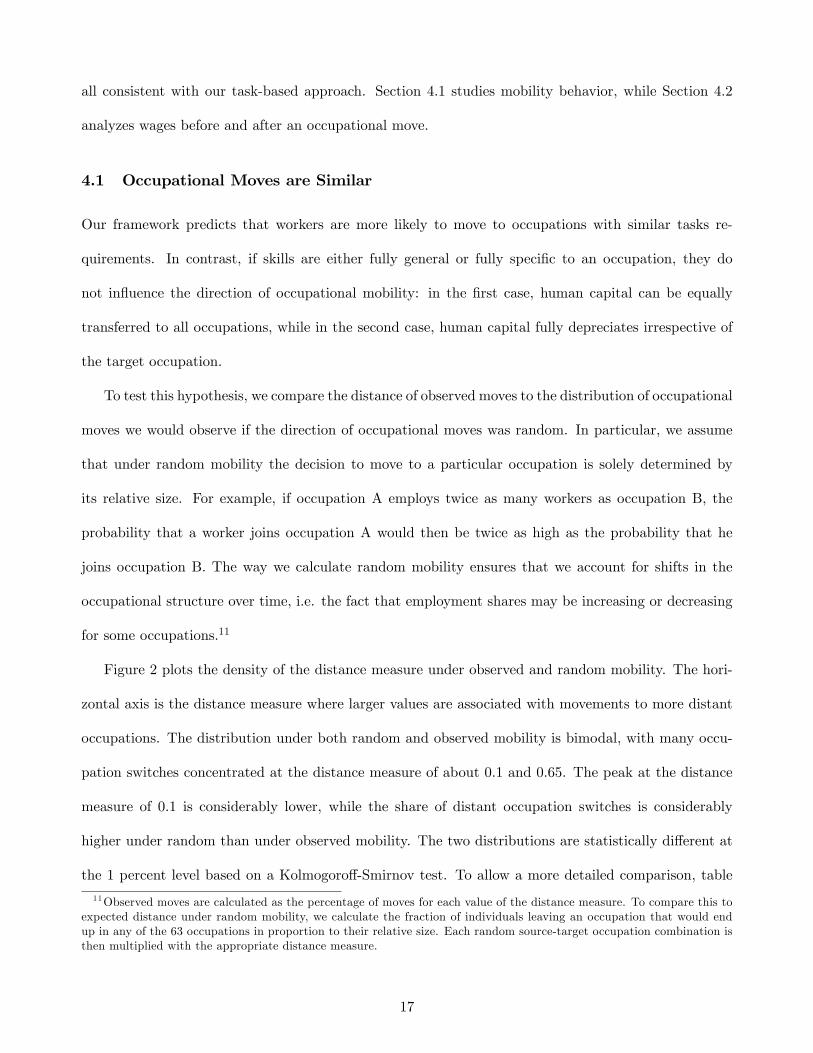
To test this hypothesis, we compare the distance of observed moves to the distribution of occupational

moves we would observe if the direction of occupational moves was random. In particular, we assume

that under random mobility the decision to move to a particular occupation is solely determined by

its relative size. For example, if occupation A employs twice as many workers as occupation B, the

probability that a worker joins occupation A would then be twice as high as the probability that he

joins occupation B. The way we calculate random mobility ensures that we account for shifts in the

occupational structure over time, i.e. the fact that employment shares may be increasing or decreasing

for some occupations.11

Figure 2 plots the density of the distance measure under observed and random mobility. The hori-

zontal axis is the distance measure where larger values are associated with movements to more distant

occupations. The distribution under both random and observed mobility is bimodal, with many occu-

pation switches concentrated at the distance measure of about 0.1 and 0.65. The peak at the distance

measure of 0.1 is considerably lower, while the share of distant occupation switches is considerably

higher under random than under observed mobility. The two distributions are statistically di¤erent at

the 1 percent level based on a Kolmogoro¤-Smirnov test. To allow a more detailed comparison, table

11Observed moves are calculated as the percentage of moves for each value of the distance measure. To compare this toexpected distance under random mobility, we calculate the fraction of individuals leaving an occupation that would endup in any of the 63 occupations in proportion to their relative size. Each random source-target occupation combination isthen multiplied with the appropriate distance measure.

17

4 compares selected moments of the distribution of our distance measure under observed and random

mobility. The observed mean and the 10th, 25th, 50th, 75th and 90th percentile of the distance dis-

tribution are much lower than what we would observe under random mobility. Figure 2 and table 4

both show that empirically observed moves are much more similar than we would expect if occupational

mobility was determined by relative size alone.

Our framework also predicts that distant moves occur early in the labor market career and moves

become increasingly similar with time in the labor market. One reason is that the accumulation of

task-speci�c skills makes distant occupational switches increasingly costly. A second reason is that with

time in the labor market, workers gradually locate better and better occupational matches. It therefore

becomes less and less likely that they accept o¤ers from very distant occupations.

Table 5 provides empirical support for these predictions. It shows the results from a linear regression

where the dependent variable is the distance of an observed move separately by education group. Column

(1) controls for experience and experience squared and year and occupation dummies. For all education

groups, the distance of an occupational move declines with time spent in the labor market though at a

decreasing rate. The declining e¤ect is strongest for the high-skilled, who also make more similar moves

on average (see last row). For the high-skilled, 10 years in the labor market decrease the distance of a

move by 0.16 or about 70 percent of the standard deviation. For the medium-skilled, the decline is only

about 0.03 or 14 percent of a standard deviation.

Furthermore, more time spent in the previous occupation decreases the distance of an occupational

move in addition to labor market experience (column (2)). Column (3) reports the results from an

�xed-e¤ects estimator to control for heterogeneity in mobility behavior across individuals. The within

estimator shows that occupational moves become more similar even for the same individual over time.

If anything, the pattern of declining distance is more pronounced in the �xed e¤ects estimation.

Table 5 imposed a quadratic relationship between actual labor market experience and the distance

of moves. In �gure 3, we relax this restriction. The �gure displays the average distance of a move by

actual experience, separately for the three education groups. The average distance is obtained from a

18

least-squares regression of the distance on dummies for actual experience as well as occupation and year

dummies, similar to Column (1) in table 5. The �gure shows that occupational moves become more

similar with time in the labor market for all education groups, but particularly so for the high-skilled in

the �rst 5 years in the labor market. The decline in distance between the �rst and 15th year of actual

labor market experience is statistically signi�cant at the 1 percent level for all education groups.

In sum, individuals are more likely to move to occupations in which similar tasks are performed as

in their source occupation, particularly so later in their career. These patterns are consistent with our

view that human capital is task-speci�c and hence, more transferable between occupations with similar

skill requirements.

4.2 Wages in Current Occupation Depend on Distance of Move

If skills are task-speci�c and hence partially transferable across occupations, this should also be re�ected

in the wages of occupational movers. Speci�cally, we expect that wages in the new occupation are more

highly correlated with wages in the source occupation if the two require similar skills. The reason is

that the wage in the previous occupation in part re�ects task-speci�c human capital, which is valuable

in the new occupation. In our data, we only observe occupational moves for workers who chose to move

a nearby or distant occupation, and the correlation between wages in the source and target occupation

is likely to be di¤erent for these workers than for workers who are forced to move to a nearby or

distant occupation. We wish to stress, however, that despite the endogenous selection of workers into

occupations, a decline in the correlation with the distance of the move is consistent with our task-based

approach.

Table 6 investigates whether the correlation of wages before and after an occupational move indeed

declines with the distance of a move. It reports estimates from a wage regression where the dependent

variable is the log daily wage. All speci�cations include experience and experience squared as well as

year and occupation dummies. Compared to the benchmark of occupational stayers (column (1)), the

correlation of wages is much lower for our sample of occupational movers (column (2)).

19

The third speci�cation (column (3)) adds the distance of the move as well as the distance interacted

with the wage at the source occupation as additional regressors. As expected, wages in the source

occupation are a better predictor for wages in the new occupation if the occupations require similar

skills. For the high-skilled, our estimates imply that the correlation of the wage at the source occupation

and the wage at the target occupation is 0.35 for the most similar move, 0.31 for the median move

(0:351� 0:103� 0:354), and approaches 0 for the most distant move (0:352� 0:939� 0:354).

If skills are partially transferable across occupations, time spent in the last occupation should also

matter for wages in the new occupation, especially if the two occupations require similar skills. In

Column (1) of table 7, we regress wages at the new occupation on occupational tenure at the previous

occupation and the same controls as before. Past occupational tenure positively a¤ects wages at the

new occupation.

Column (2) adds the distance measure interacted with past occupational tenure as controls. As

expected, the predictive power of past occupational tenure is stronger if source and target occupations

are similar, especially for university graduates. For the high-skilled, the impact of past occupational

tenure on wages is 2.3 percent for the most similar move, but only 1 percent (0:023 � 0:103� 0:072 =

0:010) for the median move.

Figure 4a relaxes the assumption that the correlation between wages across occupations declines

linearly with the distance. The x-axis shows the distance with one being the most similar occupational

moves and 10 the most distant ones, while the y-axis reports the coe¢ cient on the wage in the source

occupation for each of the 10 categories.12 Figure 4b provides a similar analysis for past occupational

tenure. The y-axis are now the coe¢ cients on the 9 distance measure dummies from a tobit regression

that also controls for actual experience, actual experience squared and year dummies.

Two things are noteworthy: �rst, the �gures highlight that the source occupation has a stronger

explanatory power for the wage at the target occupation if the source and the target occupation have

12The coe¢ cient is obtained form a OLS regression (tobit regression for the high-skilled) that controls for actual expe-rience, actual experience squared, year dummies, the wage at the source occupation, 9 dummies for the distance of themove and the 9 dummies interacted with the wage at the source occupation (see column (3) in table 6).

20

similar skill requirements. Second and in line with our results on mobility and wages, the decline is

strongest for the high-skilled. For this education group, the partial correlation coe¢ cient between wages

in the source and target occupation drops from 37 percent for the 10 percent most similar moves to

around 15 percent for the 10 percent most distant moves. The drop is statistically signi�cant at a one

percent level for all education groups.

We have performed a number of robustness checks. First, results for alternative distance measures

are very similar. Second, our sample of movers contains both occupational switches between �rms as

well as within the same �rm. The latter account for roughly 10 percent of all occupational movers. If

some skills are tied to a �rm, internal movers would have more portable skills than �rm switchers. We

therefore reestimated our speci�cations in table 5 to 7 using only external movers. The results exhibit

the same patterns in mobility and wages which we observe for the whole sample of movers. Finally,

our original sample of movers contains everybody switching occupations irrespective of the duration

of intermediate un- or nonemployment spells. To account for potential heterogeneity between those

remaining out of employment for an extended period of time and job-to-job movers, we reestimated the

results only for the sample of workers with intermediate un- or nonemployment spells of less than a

year. Again, this does not change the patterns on mobility and wages.

4.3 Can these Patterns be Explained by Unobserved Heterogeneity?

The strong patterns in mobility and wages reported in the last section support our view that human

capital accumulated in the labor market is portable across occupations, and the more so the more similar

are the occupations. This section discusses whether our �ndings could be rationalized by individual

unobserved heterogeneity.

Note �rst that all results presented above are based on a sample of occupational movers. The

patterns in mobility and wages can therefore not be accounted for by a simple mover-stayer model,

where movers have a higher probability of leaving a job and therefore lower productivity because of less

investment in speci�c skills. To the extent that movers di¤er from stayers in terms of observable and

21

unobservable characteristics, this sample restriction reduces selection bias.

However, other sources of unobserved heterogeneity could bias our results. First, suppose that high

ability workers are less likely to switch occupations. This could account for the fact that the time spent

in the last occupation has a positive e¤ect on wages in the current occupation, as past occupational

tenure would act as a proxy for unobserved ability in the wage regression (see table 7). However,

unobserved ability per se cannot explain why the e¤ect of past occupational tenure should vary with

the distance of the move or why individuals move to similar occupations at all.

First, one might argue that similar moves in the data are voluntary transitions, while distant movers

are �lemons� that are laid from their previous job and cannot �nd jobs in similar occupations. The

distinction between quits and layo¤s could explain why wages are more highly correlated across similar

occupations or why past occupational tenure has a higher return in a similar occupation. However,

the distinction between voluntary and involuntary movers cannot explain why voluntary movers choose

similar occupations in the �rst place.

We checked whether our results di¤er between job-to-job movers, which are more likely to be volun-

tary, and job-to-unemployment transitions, which are more likely to be involuntary. While the distance

of moves is lower for job-to-job transitions, we �nd similar patterns for mobility and wages for the two

types of movers. Hence, di¤erences between voluntary and involuntary occupational movers cannot

account for our �ndings.

Finally, suppose that the sample of movers di¤ers in their taste for particular tasks. Some individuals

prefer research over negotiating, while other prefer negotiating over managing personnel etc. Taste

heterogeneity can explain why we see similar moves in the data. If individuals choose their occupations

based on earnings and preferences for tasks, individuals would want to move to occupations with similar

task requirements. However, a story based on taste heterogeneity alone cannot explain why wages are

more strongly correlated between similar occupations. If there are compensating wage di¤erentials, we

would actually expect the opposite result: individuals would be willing to accept lower wages in an

occupation with their preferred task requirements.

22

This discussion highlights that a simple story of unobserved heterogeneity cannot account for all

of the results presented above. The next section outlines an estimation approach to quantify the

importance of task-speci�c human capital for individual wage growth that takes into account workers�

decision whether to switch occupations, and whether to move to a close or distant occupation.

5 Task-Speci�c Human Capital and Individual Wage Growth

To estimate the contribution of task-speci�c human capital to individual wage growth, we start from

the log-wage regression (equation (1) in Section 2) augmented by control variables eXiot:lnwiot = 1oExpit + 2oOTiot + 3oTTiot + �

0 eXiot + uiot; (2)

uiot = �oTAi + (1� �o)TMi + "iot:

Here Expit denotes actual experience, OTiot occupation tenure, and TTiot task tenure, capturing gen-

eral, occupation- and task-speci�c human capital accumulation respectively. 1o; 2o; 3o denote the

occupation-speci�c return to the three types of human capital. eXiot captures other control variables(year, occupation and region dummies) with the common return �. The unobserved (for the econome-

trician) error term uiot consists of the task-speci�c match in an occupation (�oTAi + (1 � �o)TMi ) and

an iid error term ("iot).

Our goal here is to identify the average return to the three types of human capital across occupations,

ko = Eo[ ko]; k = 1; 2; 3: Rewriting equation (2) as a random coe¢ cient model:

lnwiot = 1Expit + 2OTiot + 3TTiot + �0 eXiot + euiot; (3)

euiot = ( 1o � 1)Expit + ( 2o � 2)OTit + ( 3o � 3)TTit + �oTAi + (1� �o)TMi + "iot:

The unobserved error term euiot now contains an additional term capturing the occupational heterogene-ity in the return to the three types of human capital accumulation.

23

The next section presents our benchmark least squares results. We then discuss how to get consistent

estimates of (3) in the presence of endogenous selection into occupations: �rst, we use a sample of

displaced workers and second, we outline a control function approach to model endogenous selection.

Section 5.3. shows the economic signi�cance of our results, while Section 5.4 discusses the robustness

to alternative speci�cations.

5.1 Least Squares Results

This section discusses our benchmark least squares results; for university graduates, we estimated

censored regression models to account for topcoded wages. Table 8 reports results for the whole sample

and the sample of �rm switchers. The �rst speci�cation (odd columns) displays results from a wage

regression that ignores task-speci�c human capital, while even columns includes task tenure as an

additional regressor.

The results (columns (1) to (4)) reveal several interesting patterns. Returns to task tenure are

sizeable and exceed those of occupational tenure for all education groups. A second interesting result

is that the returns to more speci�c and general human capital decline once we account for task-speci�c

human capital. More speci�cally, returns to occupational tenure decline by about 33 percent, while

returns to experience go down by 30 percent for high-skilled workers with 10 years of experience. This

result is consistent with our view that human capital is partially transferable across occupations.

While these patterns are suggestive, least squares estimates of (3) su¤er from two biases. First,

individuals select into a new occupation based on the value of their task match, �oTAi + (1 � �o)TMi :

The second source of bias is that individuals select into occupations based on the returns to their skills

( 1o; 2o; 3o).13

13We expect the average return to experience, 1; to be upward biased because worker locate better matches with time inthe labor market through on-the-job search. Hence, the return to experience does not only re�ect accumulation of generalhuman capital, but also wage growth due to job search (see also Topel, 1991; Dustmann and Meghir, 2005). In contrast,the return to occupation- and task-speci�c human capital, 2 and 3; may be upward or downward biased. Workers witha good match are less likely to switch occupations, which produces a positive (partial) correlation between occupationand task tenure and the match quality. However, workers may have switched to a new occupation or moved to a distantoccupation because they found a particularly good match with the new occupation, which implies a downward bias inthe return to occupation- and task-speci�c human capital. Finally, workers may also move to a new and/or a distantoccupation because of a higher return to human capital, which provides another reason why the (partial) bias in the returnto occupation and task tenure cannot be signed.

24

Our �rst step towards eliminating these biases is to use a sample of workers who were exogenously

displaced from their job due to plant closure (see Gibbons and Katz, 1991; Neal, 1995 and Dustmann

and Meghir, 2005 for a similar strategy).14 Displaced workers di¤er from voluntary �rm switchers

because they are willing to accept a new job o¤er if its value exceeds the value of unemployment, as

opposed to the value of the old job. Hence, displaced workers lose some of their �search capital�, which

reduces the �rst source of bias from improved matches.

The last two columns in table 8 shows that task tenure remains an important source of individual

wage growth for the sample of displaced workers. The results for the low- and medium-skilled remain

very stable. For the high-skilled, the return to experience declines in the displaced sample, which sug-

gests that improvements in match quality (due to job search) are important for this group. Restricting

the sample to displaced workers does, however, not solve the problem of endogenous selection into

new occupations. We now outline a control function approach to get consistent estimates of the wage

equation.

5.2 Control Function Estimates

To account for endogenous selection into occupations, we need to explicitly model the conditional mean

of the error term in (3) (Heckman and Vytlacil, 1998). More speci�cally, we require that the following

exclusion restriction holds:

E[euiotjXiot; Ziot] = 0;where X 0

iot = [Expit OTeniot TTeniot eXiot] is the vector of regressors and Ziot denotes a vector ofinstruments. The above conditions is equivalent to

E[�oTAi + (1� �o)TMi jXiot; Ziot] = 0; and (4)

E[ 1o � 1jXiot; Ziot] = E[ 2o � 2jXiot; Zit] = E[ 3o � 3jXiot; Zit] = 0: (5)

14Dustmann and Meghir (2005) provide evidence that the assumption of plant closure as an exogenous job loss isreasonable in the German context.

25

The �rst exclusion restriction in (4) accounts for selection based on the task match, while the second

one in (5) addresses the selection into occupations based on the occupation-speci�c returns to human

capital.

As instruments, we require variables that a¤ect the worker�s mobility decision (i.e. whether to

move to a new occupation and whether to move to a similar or distant occupation), but not his wage

o¤er conditional on all regressors. Our main instruments for experience are age and age squared. To

instrument for occupation tenure, we follow Altonji and Shakotko (1987) and Parent (2000) and use the

deviation of occupation tenure from its occupation-speci�c mean as an instrument. This instrument is

uncorrelated with the time-invariant task match, �oTAi + (1� �o)TMi ; by construction.

For task tenure, we use local labor market conditions, in particular the size of occupation and the

average distance to other occupations in the same local labor market, as well as both variables interacted

with age, as instruments.15 The basic idea is that workers who have more employment opportunities

in their original occupation or similar occupations will be less likely to switch occupations or move

to a distant occupation. Since all our speci�cations include occupation, region and time dummies,

the variation we exploit is changes in the occupational structure over time within the same region.

These changes will not a¤ect wages if factor prices are equalized across local labor markets. Hence, our

assumption requires that wages are set in a national labor market (see Adda et al., 2006 for a similar

argument).

To implement the estimator, we estimate in a �rst step the reduced forms for experience, occupational

tenure and task tenure to predict the residuals. The results are shown in Table A2 for the low- and

medium-skilled and Table A3 for the high-skilled. In the second step, we estimate the log wage equation

in (3) including the estimated residuals as well as their interaction with the endogenous regressors. For

the high-skilled, we use the semiparametric estimator proposed by Blundell and Powell (2004) to account

for censoring in addition to endogenous regressors. We describe this estimator in detail in Appendix

15The average distance, ADrt, to other occupations is computed separately for each local labor market r and time periodt as follows: ADrt =

P64o0 6=oProprto0 �Distanceoo0):We de�ne a region as the individual�s county (Kreis) of residence as well

as all the neighboring counties, corresponding roughly to a 50 mile radius from the individual�s home.

26

B. To correct for generated regressor bias, we bootstrap standard errors with 100 replications using the

individual as the sampling unit.

Table 9 reports the results of our control function estimates, for a sample of �rm switchers (columns

(1) and (2)) and a sample of displaced workers (columns (3) and (4)).16 For the sample of �rm switchers,

the control function estimates yield similar returns to experience than the OLS results. The return to

occupation tenure, however, decreases and even becomes negative for the low- and high-skilled. In

contrast, the return to task tenure, however, increases considerably when the control function estimator

is used. One explanation for this �nding is that workers move to distant occupations because they are

well matched with that occupation, implying a negative correlation between task tenure and the task

match.

Results for the sample of displaced workers (columns (3) and (4)) are considerably more noisy. This

result is not too surprising given that identi�cation relies on workers who lose their job due to plant

closure more than once.17 Nevertheless, we �nd similar estimates for the low-skilled though only the

return to experience is statistically signi�cant. The e¤ect of task tenure is considerably stronger for the

medium-skilled but weaker for the small sample of high-skilled displaced workers.

Across all speci�cations, we �nd that task-human capital is an important source of individual wage

growth. Furthermore, returns to general and more speci�c human capital decline substantially once we

account for task human capital.

5.3 Economic Interpretation

How important then is task-speci�c human capital for individual wage growth over the life-cycle? The

least squares results for the displaced sample imply that a high-skilled worker can expect his wages to

grow by 36% due to human capital accumulation over the �rst ten years in the labor market (table 8,

column (6)). Task-speci�c human capital contributes 40 percent (0.023*6.19/0.36) to this wage growth,

16The coe¢ cients on the residuals and their interaction with the main regressors can be found in Table A4. Both theresiduals and the residuals interacted with the regressors enter the wage equation signi�cantly, indicating that selectioninto occupations based on the task match and occupation-speci�c returns is important.17The reason is that for workers who experienced only one plant closure our instrument for occupation tenure, i.e. the

deviation from its occupation-speci�c mean, is zero.

27

experience 46 percent ((0.037*6.81-0.002*6.812)=/0.36) and occupation-speci�c human capital only 14

percent (0.01*4.95/0.36).18 A similar calculation for the medium- and low-skilled implies that task-

speci�c human capital accounts for at least 35 and 25 percent of overall wage growth, respectively.

These calculations demonstrate that task-human capital is an important source of wage growth over

the labor market career.

More generally, our results suggest that most human capital is quite portable and at least partially

transferable across occupations. This result is important for evaluating the costs of job displacement,

for example following technological change or economic restructuring more generally.

As an illustration, consider again a high-skilled worker who is displaced after 10 years in his occu-

pation. If the worker can �nd employment in an occupation with similar skill requirements (e.g. in

the 10th percentile of the distribution of moves), his overall wage loss would be 12.3 percent. Most of

this decline is due to the loss of occupation-speci�c skills while few task-speci�c human capital is lost.

However, if the worker cannot �nd employment in a similar occupation (e.g. in the 90th percentile of

the distribution of moves), his wage would decline by 30.1 percent.19 The basic pattern holds for all

education and experience groups.

These calculations highlight that wage losses of job displacement strongly depend on the thickness of

labor markets. In particular, wage losses are higher in occupations with skill requirements that are very

di¤erent from other occupations. Costs of job displacement will also be higher in an economy where

information about the task content of alternative occupations is limited. In contrast, job reallocation is

less costly if similar occupations and information about close substitute occupations are widely available.

18This calculation takes into account that after 10 years in the labor market, a high-skilled worker has accumulated 6.81years of actual experience, 4.95 years of occupation tenure, and 6.19 years of task tenure. When we base the calculationon the control function estimates for the sample of �rm switchers, task-speci�c human capital becomes the main source ofwage growth from human capital accumulation.19We again base our calculation on the least squares estimates for the displaced sample (table 8, column (6)). Note that

since our calculation excludes the loss in task match quality, our wage losses are a lower bound for the true wage loss ofjob displacement.

28

5.4 Further Robustness Checks

This section discusses three extensions to our framework: worker ability, �rm matches and job ladders.

We address each of them in turn.

Suppose workers di¤er in their general ability so that the error term in wage regression (2) does

not only consist of the task match, but also of a �xed worker e¤ect. If workers who switch to distant

occupations are of lower ability (�lemons�), then this could potentially explain our positive return to task-

human capital in the OLS regressions. Note, however, that our control function estimates account for

this bias. An alternative way to eliminate this type bias is by �rst di¤erencing. As a further robustness

check, we report �rst di¤erence estimates for the sample of �rm switchers in table 9, columns (5) and (6).

Since we cannot estimate �rst di¤erences for university graduates, we use Honoré�s trimming estimator

(1992) for censoring (Type 1 tobit model) with �xed e¤ects instead.20 While the �rst di¤erence estimates

for occupation- and task tenure are somewhat smaller than the OLS and control function estimates,

task tenure remains a signi�cant source of individual wage growth even after accounting for general

worker ability.21

Our wage speci�cation (3) does not incorporate job search over �rm matches which has been shown

to be an additional source of wage growth (e.g. Topel and Ward, 1991; Pavan, 2005; Yamaguchi, 2007b).

How would �rm matches a¤ect our �ndings? Neal (1999) proposes a model in which workers search

over both �rm and occupation matches. He shows that it is optimal for workers to �rst search for a

good occupation match, and then for a good �rm match. For a sample of young workers like ours, he

then provides empirical support for such a search strategy. Under the two-stage search strategy, our

estimates will be little a¤ected by search over �rm matches. The reason is that the majority of young

workers in our sample has been in the labor market for less than 8 years so their decision whether to

switch occupations and to which occupation to move should be predominantly driven by the task match,

20Since the estimator is semiparametric, no functional form assumption on the error term is required. However, we dorequire pairwise exchangeability of the error terms conditional on the included regressors (see Honoré 1992 for details).21Note that due to di¤erences in the econometric model, the results for the low- and medium-skilled cannot be directly

compared to those of the high-skilled. Also note that in the �rst di¤erence regression, the coe¢ cient on (the change in)experience should not be interpreted as returns to general human capital accumulation, as they additionally re�ect thechange in the �rm and task match quality.

29

and not by the �rm match.

What if the worker�s search strategy does not follow this two-stage rule? Then �rm matches provide

another reason why in an OLS regression the return to task tenure may be downward biased because

some workers may have moved to a distant occupation because of a high �rm match, despite a low task

match.

In addition to �rm matches, we have also abstracted from occupational mobility along a job ladder

(see Gibbons et al., 2005; Jovanovic and Yarkow, 1997; Yamaguchi, 2007a). Within our framework,

job ladders can be modeled by relaxing the restriction that the occupation-speci�c weights add up to

one. We would expect occupations that have a higher analytic and manual weight to be higher up the

job ladder, and workers should move along the ladder as they become more experienced. While we

do not explicitly analyze hierarchical occupation mobility in this paper, our control function estimates

is consistent even in the presence of career mobility. This is because the validity our instruments, in

particular the deviation of occupation tenure from its occupation-speci�c mean, does not rely on the

assumption that the occupation-speci�c weights add up to one.

6 Conclusion

How general is human capital? The evidence in this article demonstrates that speci�c skills are more

portable than previously considered. We show that workers are much more likely to move to occupations

that require similar skills and that the distance of occupational moves declines over the life-cycle.

Furthermore, wages and occupation tenure at the source occupation have a stronger impact on current

wages if workers switch to a similar occupation.

The evidence also suggests that task-speci�c human capital is an important source of individual wage

growth, in particular for university graduates. For them, at least 40 percent of wage growth due to

human capital accumulation can be attributed to task-speci�c human capital, while occupation-speci�c

skills and experience account for 14 and 47 percent respectively. For the medium-skilled (low-skilled),

at least 25 (35) percent of individual wage growth is due to task-speci�c human capital. We also provide

30

evidence that the costs of displacement and job reallocation depend on the employment opportunities

after displacement: Wage losses are lower if individuals are able to �nd employment in an occupation

with similar skill requirements.

Our �ndings on both mobility patterns and wage e¤ects are strongest for the high-skilled, suggest-

ing that task-speci�c skills are especially important for this education group. One explanation for this

pattern is that formal education and task-speci�c human capital are complements in production. Com-

plementarity implies that high-skilled workers accumulate more task human capital on the job which

would account for the sharp decline in the distance of moves over the life cycle. It would also explain

why wages in the previous occupation are less valuable in the new occupation and why returns to task

human capital are higher than for the two other education groups.

The results in this paper are di¢ cult to reconcile with a standard human capital model with fully

general or �rm- (or occupation-) speci�c skills. Our �ndings also contradict search models where the

current occupation has no e¤ect on future occupational choices, and skills are not transferable across

occupations. The �ndings however support a task-based approach to modeling labor market skills in

which workers can transfer speci�c human capital across occupations.

References

[1] Abraham, K. G., and H. S. Farber (1987), �Job Duration, Seniority, and Earnings,�American

Economic Review, 77, 278-97.

[2] Adda, J., Dustmann, C., Meghir, C., and J.-M. Robin (2006), �Career Progression and Formal

versus On-the-Job Training,�IZA Discussion Paper No. 2260.

[3] Altonji, J. and R. Shakotko (1987), �Do Wages Rise with Job Seniority?,�Review of Economic

Studies, 54, 437-59.

[4] Altonji, J. and N. Williams (2005), �Do Wages Rise with Job Seniority? A Reassessment,�Indus-

trial and Labor Relations Review, 58, 370-97.

[5] Autor, D., R. Levy and R.J. Murnane (2003), �The Skill Content of Recent Technological Change:

An Empirical Investigation�, Quarterly Journal of Economics, 118, 1279-1333.

[6] Becker, G.S. (1964), Human Capital, University of Chicago Press.

[7] Ben-Porath, Y. (1967), �The Production of Human Capital and the Life-Cycle of Earnings,�Journal

of Political Economy, 75, 352-65.

31

[8] Blundell, R. and J. Powell (2004), �Censored Regression Quantiles with Endogenous Regressors�,

mimeo, University of California at Berkeley.

[9] Borghans, L., B. ter Weel and B.A. Weinberg (2006), �Interpersonal Styles and Labor Market

Outcomes, �mimeo, Maastricht University.

[10] DiNardo, J. and J.-S. Pischke (1997), �The Returns to Computer Use Revisited: Have Pencils

Changed the Wage Structure Too?,�Quarterly Journal of Economics, 112, 291-303.

[11] Dustmann, C. and C. Meghir (2005), �Wages, Experience and Seniority,� Review of Economic

Studies, 72, 77-108.

[12] Farber, H. (1999), �Mobility and Stability: The Dynamics of Job Change in Labor Markets,� in:

Handbook of Labor Economics, volume 3, edited by O. Ashenfelter and D Card, Elsevier Science.

[13] Fitzenberger, B. and A. Kunze (2005), �Vocational Training and Gender: Wages and Occupational

Mobility among Young Workers,�Oxford Review of Economic Policy, 21, 392-415.

[14] Fitzenberger, B. and A. Spitz-Öner (2004), �Die Anatomie des Berufswechsels: Eine empirische

Bestandsaufnahme auf Basis der BiBB/IAB-Daten 1998/99,� in: W. Franz, H.J. Ramser und

M. Stadler, Bildung, Wirtschaftswissenschaftliches Seminar in Ottobeuren, Bd. 33, Tübingen,

29-54.

[15] Flinn, C. (1986), �Wages and Job Mobility of Young Workers,�Journal of Political Economy, 84,

S88-S110.

[16] Gibbons, R. and L.F. Katz (1991): �Layo¤s and Lemons,�Journal of Labor Economics, 9, 351-80.

[17] Gibbons, R.; L.F. Katz; T. Lemieux and D. Parent (2005): �Comparative Advantage, Learning

and Sectoral Wage Determination,�Journal of Labor Economics, 23, 681-724.

[18] Gibbons and Waldman (2004), �Task-Speci�c Human Capital,�American Economic Review P&P,

94, 203-207.

[19] Gibbons, R. and M. Waldman (2006), �Enriching a Theory of Wage and Promotion Dynamics

inside Firms,�Journal of Labor Economics, 24, 59-107.

[20] Heckman, J.J. and G. Sedlacek (1985), �Heterogeneity, Aggregation, and Market Wage Functions:

An Empirical Model of Self-Selection in the Labor Market,�Journal of Political Economy, 93:

1077-1125.

[21] Heckman, J.J. and E. Vytlacil (1998), �Instrumental Variables Methods for the Correlated Random

Coe¢ cient Model,�Journal of Human Resources, 1998, 33, 974-1002.

[22] Honoré, B. (1992), �Trimmed LAD and Least Squares Estimation of Truncated and Censored

Regression Models with Fixed E¤ects,�Econometrica, 60, 533-65.

[23] Ingram, B.F. and G. Neumann (2006), �The Return to Skill,�Labour Economics, 13: 35-59.

[24] Ja¤e, A.B. (1986),�Technological Opportunity and Spillover of R&D: Evidence from Firms�Patents,

Pro�ts, and Market Value,�American Economic Review, 76, 984-1001.

[25] Jovanovic, B. (1979a), �Firm Speci�c Capital and Turnover,� Journal of Political Economy, 87,

1246-60.

32

[26] Jovanovic, B. (1979b), �Job Matching and the Theory of Turnover,�Journal of Political Economy,

87, 972-90.

[27] Jovanovic, B. and Y. Yarkow (1997), �Stepping-Stone Mobility�, Carnegie-Rochester Series of

Public Policy, 46, 289-325.

[28] Kambourov, G. and I. Manovskii (2007a), �Occupational Mobility and Wage Inequality,�Review

of Economic Studies, forthcoming.

[29] Kambourov, G. and I. Manovskii (2007b), �Occupational Speci�city of Human Capital,� Interna-

tional Economic Review, forthcoming.

[30] Kletzer, L. (1989), �Returns to Seniority after Permanent Job Loss,�American Economic Review,

79, 536-53.

[31] Lazear, E.P. (2003), �Firm-Speci�c Human Capital: A Skill-Weights Approach,�NBER Working

Paper W9679.

[32] Ljungqvist, L. and T.J. Sargent (1998), �The European Unemployment Dilemma,� Journal of

Political Economy, 106, 514-550.

[33] Malamud, O. (2005), �Breadth vs. Depth : The E¤ect of Academic Specialization on Labor Market

Outcomes,�Harris School Working Paper Series 05.17.

[34] McCall, B.P. (1990), �Occupational Matching: A Test of Sorts,�Journal of Political Economy, 98:

45-69.

[35] Miller, R. (1984), �Job Matching and Occupational Choice,� Journal of Political Economy, 92:

1086-1120

[36] Mincer, J. (1974), Schooling, Experience and Earnings, Columbia University Press.

[37] Murphy, K.M. (1986), �Specialization and Human Capital,�Unpublished Dissertation, University

of Chicago.

[38] Neal, D. (1995), �Industry-Speci�c Capital: Evidence from Displaced Workers,�Journal of Labor

Economics, 13: 653-77.

[39] Neal, D. (1999), �The Complexity of Job Mobility among Young Men,�Journal of Labor Economics,

17: 237-61.

[40] Parent, D. (2000), �Industry-Speci�c Capital and the Wage Pro�le: Evidence from the National

Longitudinal Study of Income Dynamics,�Journal of Labor Economics, 18: 306-23.

[41] Pavan, R. (2005), �Career Choice and Wage Growth,�mimeo, University of Chicago.

[42] Poletaev, M. and C. Robinson (2008) , �Human Capital Speci�city: Evidence from the Dictionary

of Occupation Titles and Displaced Worker Surveys, 1984-2000,�Journal of Labor Economics,

26, 387-420.

[43] Rosen, S. (1983), �Specialization and Human Capital,�Journal of Labor Economics, 1, 43-49.

[44] Roy, A.D. �Some Thoughts on the Distribution of Earnings,�Oxford Economic Papers, 3, 135-146.

[45] Shaw, K. (1984), �A Formulation of the Earnings Function Using the Concept of Occupational

Investment,�Journal of Human Resources, 19. 319-340.

33

[46] Shaw, K. (1987), �Occupational Change, Employer Change, and the Transferability of Skills,�

Southern Economic Journal, 53: 702-19.

[47] Spitz-Öner, A. (2006), �Technical Change, Job Tasks, and Rising Educational Demands: Looking

Outside the Wage Structure,�Journal of Labor Economics, 24, 235-70.

[48] Topel, R. (1991), �Speci�c Capital, Mobility and Wages: Wages Rise with Job Seniority,�Journal

of Political Economy, 99, 145-76.

[49] Topel, R. and M. Ward (1992), �Job Mobility and the Careers of Young Men,�Quarterly Journal

of Economics, 107, 439-80.

[50] Violante, G.L. (2002), �Technological Acceleration, Skill Transferability, and the Rise in Residual

Inequality,�Quarterly Journal of Economics, 117, 297-338.

[51] Wasmer, E. (2004), �Interpreting Europe and US Labor Markets Di¤erences: The Speci�city of

Human Capital Investments,�American Economic Review, 96, 811-831.

[52] Yamaguchi, S. (2007a), �Career and Skill Formation: A Dynamic Occupational Choice Model with

Multidimensional Skills,�mimeo, McMaster University.

[53] Yamaguchi, S. (2007b), �The E¤ect of Match Quality and Speci�c Experience on Career Decisions

and Wage Growth,�mimeo, McMaster University.

A Data Sources

A.1 Data on Occupational Tasks (1979-1999)

We use four cross-sections of the German Quali�cation and Career Survey conducted in 1979, 1985,

1991/92 and 1998/99 by the Federal Institute of Vocational Training (BIBB) and the Institute for Labor

Market Research (IAB). The data with a sample size of 30,000 covers individuals between 16 and 65,

who are employed at the time of the survey. We restrict our sample to men employed in West Germany

and exclude the self-employed, civil servants and those working in agriculture. We also exclude those

without German nationality since they were not included in each wave. We use the same 64 occupations

based on a classi�cation system by the Federal Employment O¢ ce, which is standardized over time.

The aggregation at the 2-digit level decreases well-known measurement error problems of occupational

classi�cations in survey data and allows us to match the data to our main data set on job histories.

For each respondent, we know whether the worker performs certain tasks in his job and whether

this is his main activity on the job. Unlike the Dictionary of Occupational Titles (DOT) in the United

States, we do not know how intensively a particular task is used beyond the distinction of main activity,

task performed and not performed. Overall, we have information on 19 di¤erent tasks workers perform

in their jobs. Following Autor et al. (2003), we group the 19 tasks into three groups of tasks: ana-

lytical tasks, manual tasks and interactive tasks. The assignment of tasks is as follows: manual tasks

(equip or operate machines, repair, reconstruct or renovate, cultivate, manufacture, cleaning, serve or

accommodate, construct or install, pack or ship or transport, secure, nurse or treat others), analytical

tasks (research or evaluate or measure, design or plan or sketch, correct texts or data, bookkeeping or

34

calculate, program, execute laws or interpret rules) and interactive tasks (sell or buy or advertise, teach

or train others, publish or present or entertain, employ or manage personnel or organize or coordinate).

A.2 Employee Sample (1975-2001)

Our main data set is a two percent sample of all German social security records administered by the

Institute for Employment Research. By law, employers are required to report the exact beginning and

end of any employment relation of new hires and employees leaving the �rm which are subject to social

security contributions. In addition, employers provide information about all their employees at the end

of each year. We therefore know the exact date of employer changes and movements into and out of

paid employment. Another advantage is that the data contain an unusually in-depth set of background

information for each individual, including his age, education, gender, nationality, plant of work and

occupation. We distinguish three education levels: low-, medium-, and high-skilled. We de�ne a worker

to be high-skilled if at least one spell classi�es him as a graduate from a university or technical college.

(Fachhochschule). A worker is medium-skilled if he spent at least 450 days in apprenticeship training,

and no spell classi�es him as a college graduate. A worker is low-skilled if he spent less than 450 days in

apprenticeship training and did not attend a technical college or university. The occupational categories

of employees and apprentices in the social security records are highly accurate as the classi�cation forms

the basis of wage agreements between unions and employers�association. To make the 130 di¤erent

occupations we observe in our sample comparable to the BIBB data, we aggregated them into 64

occupations at the 2-digit level using a code provided to us by the Institute for Employment Research.

All experience and tenure variables refer to the beginning of each spell. Time out of the labor force and

time in unemployment as well time in apprenticeship training is not counted. If an employee returns to

his occupation, we count the time spent in the earlier spell towards his occupational tenure. The same

holds in the unlikely event that a worker returns to a �rm he has worked for previously. Our results on

occupational movers exclude these return movers, but the estimates are similar if they are included.

In addition to the sample restrictions mentioned in the text, we dropped all spells in vocational

training and those job spells that started prior to an apprenticeship or tertiary education. In addition,

we excluded observations that were still in vocational training at the end of the sample period in 2001

or pursued more than one apprenticeship, that is were employed as an apprentice for more than 7 years.

We also require a person to be below a certain age when we �rst observe them. This ensures that we

can follow them from day one of their entry into the labor market. The age restriction is 19 if the

individual has no high school degree (Abitur), 22 if the individual has a high school degree, but no

higher degree, 28 if the individual graduated from a community college (Fachhochschule), and 30 if he

graduated from university. Finally, we drop all observations we observe less than a year, with missing

education or nationality, and observations with no valid wage or a daily (real) wage below 20 DM during

an employment spell. To estimate the returns to di¤erent types of human capital in Section 5, we use

a sample of displaced workers. A worker is displaced from his �rm due to plant closure if he left the

�rm in the year or one year before the �rm closed down. As a robustness check, we have repeated the

analysis restricting the sample to workers who have left the �rm in the year or one or two year before

the �rm closed down. The �rst de�nition has the advantage that it includes less workers who have left

the �rm voluntarily, for reasons other than plant closure. It has the disadvantage that it may exclude

35

workers that leave the �rm prior to plant closure, anticipating that the �rm may shut down in the

future. Both de�nitions give very similar results.

B Blundell and Powell (2004) Control Variable Estimator

For the high-skilled, the control variable estimates in Table 9, columns (1) to (4) are based on the

semiparametric estimator proposed by Blundell and Powell (2004). This estimator accounts for censoring

in addition to endogenous regressors. It does so however at the price of imposing common returns on

the observable human capital variables. For simplicity, we drop the subscript o: The model is

lnWit = minfXit� + uit; ctg

where Xit are the endogenous regressors, uit is the scalar error term and ct is the time-dependent

censoring point. For notational convenience, we suppress all exogenous regressors here. The reduced

form links the instruments Zit to the endogenous regressors:

Xit = Zit + vit

where vit is a scalar error term and the unknown coe¢ cient vector with suitable dimensions. Instead

of imposing independence between (uit; vit) and Zit, the estimator imposes a weaker conditional quantile

exclusion restriction

Fu(qjXit; Zit) � Prfuit � qjXit; Zitg = Prfuit � qjvitg = Fu(qjvit) q 2 R

This assumption implies that the dependence of the regressors Xiot and the error term uit is driven by

the residuals vit (control variable). To consistently estimate the reduced-form above, we also require

that E[vitjZit] = 0. The estimation then proceeds as follows: �rst, we predict cvit from regressions of

the endogenous regressors on the instruments and other control variables. Then, we estimate a quantile

regression of the dependent variables on both the endogenous regressors and the instruments as well

as the control variables to obtain the �tted values \lnWit. The second step is to estimate a weighted

least squares regression of all pairwise di¤erences of the predicted dependent variable \lnWit on the

endogenous regressors Xit. The weights are the pairwise di¤erences of the residuals cvit, which are usedas inputs into a multivariate kernel function. Formally, the second-stage estimator is de�ned as

b� =

24Xs<t

Xi<j

Kv

�cvis � cvjthn

�ctisctjt(Xis �Xjt)0(Xis �Xjt)35�1 �

24Xs<t

Xi<j

Kv

�cvis � cvjthn

�ctisctjt(Xis �Xjt)0([lnW is �[lnW jt)

35where Kv(�) is the kernel function and hn is a sequence of scalar bandwidth terms. ctis is a �trimming�term, constructed so that ctis = 0 unless the estimated quantiles [lnW is > 0 and Xis and vis fall in

some compact set S. We used the product epanechnikov kernel and a separate bandwidth hn for each

36

endogenous variable. Standard errors are bootstrapped using 100 replications.

37

Mean Std.Dev Example: Teacher Example: Baker

Analytical Tasks 55.02 49.75 63.73% 32.42%Research, evaluate or measure 25.11 43.37 34.02% 13.56%Design, plan or sketch 10.21 30.28 17.62% 3.60%Correct texts or data 23.85 42.62 39.64% 6.36%Calculate or bookkeeping 26.02 43.87 11.34% 22.46%Program 8.35 27.66 8.43% 0.42%Execute laws or interpret rules 7.85 26.89 17.24% 0.85%Analytical is Main Task 31.56 46.48 15.93% 13.14%

Manual Tasks 72.42 44.69 25.59% 96.40%Equip or operate machines 19.98 39.99 7.03% 27.12%Repair, renovate or reconstruct 31.38 46.40 8.15% 10.38%Cultivate 1.77 13.19 2.25% 1.91%Manufacture, install or construct 11.97 32.46 1.97% 87.92%Cleaning 3.50 18.38 1.78% 6.14%Serve or accommodate 1.21 10.92 0.28% 3.60%Pack, ship or transport 18.76 39.04 2.72% 15.25%Secure 15.72 36.40 7.22% 18.01%Nurse or treat others 9.76 29.67 11.53% 7.84%Manual is Main Task 57.46 49.44 10.50% 88.77%

Interactive Tasks 48.48 49.98 95.31% 44.07%Sell, buy or advertise 29.21 45.48 12.00% 16.53%Teach or train others 17.15 37.69 91.38% 34.32%Publish, present or entertain others 9.58 29.43 26.24% 3.81%Employ, manage personnel, organize, coord 37.09 48.31 39.36% 29.87%Interactive is Main Task 27.55 44.68 85.94% 14.83%

Observations 52,718 1,067 472

Source : Qualification and Career Survey: 1979, 1985, 1991/2, 1997/8

Notes : The table reports the percentage of individuals in the career survey that report performing the type of task in their job. We grouped the19 different tasks into three task groups (analytical, manual and interactive skills) following Autor et al. (2003) and Spitz (2006). The fraction formain tasks sum to more than 100 percent as around 10 percent reported performing more than one main task. The last two columns show thedistribution of task usage for two common occupations: teachers (which exclude university or technical college professors) and baker.

Table 1: Summary Statistics of Task Data

Occupation 1 Occupation 2 Distance

Mean 0.244Standard Deviation 0.221

Most Similar (all Education Groups)Paper and Pulp Processing Printer, Typesetter 0.002Wood Processing Metal Polisher 0.003Chemical Processing Plastics Processing 0.004

Most Distant (all Education Groups)Banker Unskilled Construction Worker 0.939Banker Miner, Stone-Breakers 0.935Publicists, Journalist Unskilled Construction Worker 0.933

Most Common Occupational Moves (Low-Skilled) Truck Driver, Conductor Store or Warehouse Keeper 0.029Unskilled Worker Store or Warehouse Keeper 0.267Assembler Store or Warehouse Keeper 0.372

Most Common Occupational Moves (Medium-Skilled) Chemist, Physicist Electricians, Electrical Installation 0.171Sales Personnel Office Clerk 0.077Truck Driver, Conductor Store or Warehouse Keeper 0.028

Most Common Occupational Moves (High-Skilled) Engineers Chemist, Physicist 0.037Entrepreneurs Office Clerk 0.048Accountant Office Clerk 0.080

Notes : The table shows at the top summary statistics of the distance measure as well as the three most similar and distant occupations and their corresponding distance. The distance measure is the angular separation using the 19 different tasks (see Table B1 for a list of tasks) and normalized to vary between 0 and 1. The bottom part of the table shows the three most commonly observed moves in the data by education group and the corresponding distance measure.

Distance Measure (Angular separation)

Table 2: Measuring Distances between Occupations

Low Skill Medium Skill High Skill

Percentage in Sample 16.27% 68.30% 15.43%

Age (in Years) 25.82 27.47 31.85(6.26) (5.24) (5.60)

Not German Citizen 0.32 0.052 0.047(0.47) (0.22) (0.21)

Median Daily Wage 114.39 135.32 204.23(45.44) (43.52) (61.43)

Log Daily Wage 4.66 4.89 5.19(0.45) (0.33) (0.43)

Percentage censored 0.01 0.02 0.24(0.10) (0.14) (0.43)

Actual Experience (in Years) 5.76 5.59 5.25(5.40) (4.76) (4.81)

Occupational Tenure (in Years) 3.28 3.87 3.62(4.27) (4.12) (4.07)

Firm Tenure (in Years) 2.47 2.79 2.46(3.87) (3.66) (3.33)

Task Tenure (in Years) 4.58 4.81 4.66(4.65) (4.28) (4.38)

Occupational Mobility 0.186 0.114 0.109(0.389) (0.317) (0.311)

Distance of Move 0.054 0.0525 0.0441(0.025) (0.025) (0.024)

Firm Mobility 0.236 0.18 0.18(0.425) (0.384) (0.384)

Most Common Occupations Warehouse Keeper (10%) Electrical Installation (7%) Engineer (25%)Assembler (7%) Locksmith (8%) Technician (12%)Conductor (6%) Mechanic, Machinist (6%) Accountant (9%)Unskilled Worker (4%) Office Clerk (7%) Office Clerk (8%)Office Clerk (4%) Conductor (5%) Researcher, Clergymen (5%)

Number of Observations 223,399 1,000,934 197,420Number of Individuals 18,604 78,101 17,648

Source : Employee Sample (IAB), 1975-2001

Table 3: Summary Statistics of West German Employee Panel

Notes : The table reports summary statistics for the administrativepanel data on individual labor market histories and wages from 1975 to2001. Low skilled workers are those without a vocationaldegree, medium skilled have either a high school or vocationaldegree and the highskilled have an advanced degree from a technical college or university. Experience, occupation, task and firm tenure are measured fromactual spells and exclude periods of unemploymentor out of the labor force. The wage is measured in German Marks at 1995 prices and issubject to right censoring.

Random Mobility Observed Mobility

Mean 0.466 0.409

10th Percentile 0.083 0.047

25th Percentile 0.267 0.122

50th Percentile 0.507 0.381

75th Percentile 0.668 0.595

90th Percentile 0.776 0.682

Table 4: Observed Moves are More Similar than under Random Mobility

Notes : The table repports selected moments of the distribution of observed occupational moves("Observed Mobility") and compares it against what we would expect to observe under random mobility("Random Mobility"). We calculate random mobility as follows: for each mover, we assume that theprobability of going to any other occupation in the data is solely determined by the relative size of thetarget occupation. We then multiply this "random move" with its distance to get the distribution of thedistance measure under random mobility. The distance measure is the angular separation, based on19 tasks. Since all moments of the observed distribution are below those under random mobility,individuals are much more likely to move to similar occupation.

Y: Distance of Move (1) (2) (3) (1) (2) (3) (1) (2) (3)

Experience -0.005 -0.005 -0.004 -0.003 -0.003 -0.003 -0.016 -0.015 -0.017(0.001)** (0.001)** (0.002)** (0.000)** (0.000)** (0.001)** (0.001)** (0.001)** (0.003)**

Experience Squared 0.000 0.000 0.000 0.000 0.000 0.000 0.001 0.001 0.001(0.000)** (0.000)** (0.000)** (0.000)** (0.000)** (0.000)** (0.000)** (0.000)** (0.000)**

Occupation Tenure -0.003 -0.002 0.000 0.002 -0.003 0.000(0.001)** (0.001)* 0.000 (0.000)** (0.001)** -0.001

Constant 0.382 0.385 0.377 0.391 0.391 0.346 0.397 0.399 0.258(0.012)** (0.012)** (0.018)** (0.015)** (0.015)** (0.022)** (0.046)** (0.045)** (0.062)**

Year Dummies Yes Yes Yes Yes Yes Yes Yes Yes YesOccupation Dummies Yes Yes Yes Yes Yes Yes Yes Yes YesIndividual Fixed Effects No No Yes No No Yes No No YesObservations 44,149 44,149 44,149 117,206 117,206 117,206 20,947 20,947 20,947

Mean Distance of Move 0.2757 0.276 0.276 0.243 0.243 0.243 0.185 0.185 0.185(0.2255) (0.226) (0.226) (0.220) (0.220) (0.220) (0.202) (0.202) (0.202)

Notes: The table reports results from a regression where the dependent variable is the distance between two occupations. The distance measure is the angular separation, basedon 19 tasks. The sample consists of all occupational movers and results are reported separately by education group. Column (1) only includes experience and experience squared.Column (2) adds occupation tenure. Column (3) includes fixed worker effects to control for individual unobserved heterogeneity. All specifications include year and occupationdummies. Robust standard errors clustered at the individual level are reported in parentheses. Coefficients with * are statistically significant at the 5 percent level, those with ** atthe 1 percent level.

Table 5: Distance of Move Declines with Time in the Labor Market

Low-Skilled Medium-Skilled High-Skilled

Y: Log Daily Wage after Move (1) (2) (3) (1) (2) (3) (1) (2) (3)

Wage Last Period 0.783 0.220 0.252 0.787 0.328 0.381 0.890 0.296 0.351(0.004)** (0.007)** (0.010)** (0.002)** (0.004)** (0.006)** (0.005)** (0.010)** (0.011)**

Wage Last Period*Distance -0.127 -0.243 -0.354(0.023)** (0.015)** (0.032)**

Distance of Move 0.495 1.040 1.481(0.101)** (0.069)** (0.152)**

Year Dummies Yes Yes Yes Yes Yes Yes Yes Yes YesOccupation Dummies Yes Yes Yes Yes Yes Yes Yes Yes YesObservations 158,808 44,137 44,137 802,197 117,204 117,204 158,416 18,285 18,285

Notes : The table reports results from wage regressions where the dependent variable is the log daily wages at the target occupation after an occupational move. Results are reported separately by education group. For the low-and medium-skilled, we estimate OLS models. Standard errors in parentheses allow for clustering at the individual level. For the high-skilled, we estimate tobit models, and exclude censored observations at the previousoccupation. Standard errors in parentheses are bootstrapped with 100 replications to allow for clustering at the individual level. All specifications include the log daily wage in the last period, actual experience, actual experiencesquared, year and occupation dummies. Column (1) uses the sample of occupational stayers as a benchmark for comparison. Column (2) repeats the analysis for occupational movers, while Column (3) adds the distancemeasure as well as the distance measure interacted with the wage last period. The distance measure used is the angular separation based on all 19 tasks. Coefficients with * are statistically significant at the 5 percent level,those with ** at the 1 percent level.

Table 6: Similar Moves and the Correlation of Wages Across Jobs

High-Skilled Medium-SkilledLow-Skilled

Y: Log Daily Wage after Move (1) (2) (1) (2) (1) (2)

Past Occupational Tenure 0.015 0.018 0.013 0.016 0.015 0.023(0.001)** (0.001)** (0.0005)** (0.0006)** (0.002)** (0.002)**

Past Tenure *Distance -0.018 -0.022 -0.072(0.003)** (0.002)** (0.006)**

Year Dummies Yes Yes Yes Yes Yes YesOccupational Dummies Yes Yes Yes Yes Yes YesObservations 44,149 44,149 117,206 117,206 20,947 20,947

Table 7: Past Occupational Tenure Matters for Wages

Low-Skilled Medium-Skilled High-Skilled

Notes : The table reports wage regressions where the dependent variable is the log wages in the target occupation after an occupational move. Estimates arereported for each education group separately. For the low- and medium-skilled, we report results from OLS regressions. Standard errors in parentheses allow forclustering at the individual level. For the high-skilled, we estimate tobit models. Here, standard errors in parentheses are bootstrapped with 100 replications toaccount for clustering at the individual level. Column (1) in each specification controls for past tenure in the source occupation, experience, experience squared, aswell as year and occupation dummies. Column (2) additionally includes the distance measure interacted with past occupational tenure. The distance measureused is the angular separation based on all 19 tasks. Coefficients with * are statistically significant at the 5 percent level, those with ** at the 1 percent level.

(1) (2) (3) (4) (5) (6)

Panel A: Low-Skilled Task Tenure 0.012 0.024 0.020

(0.001)*** (0.001)*** (0.003)***Occupational Tenure 0.009 0.007 0.021 0.020 0.016 0.014

(0.001)*** (0.001)*** (0.001)*** (0.001)*** (0.002)*** (0.002)***Experience 0.062 0.054 0.047 0.032 0.044 0.031

(0.001)*** (0.001)*** (0.001)*** (0.002)*** (0.004)*** (0.004)***Experience Squared -0.002 -0.002 -0.002 -0.002 -0.001 -0.001

(0.000)*** (0.000)*** (0.000)*** (0.000)*** (0.000)*** (0.000)***Firm Tenure 0.008 0.007

(0.001)*** (0.001)***Observations 202,327 202,327 56,831 56,831 5,891 5,891R Squared 0.370 0.370 0.250 0.250 0.300 0.310

Panel B: Medium-Skilled Task Tenure 0.009 0.018 0.012

(0.0005)*** (0.001)*** (0.002)***Occupational Tenure 0.007 0.005 0.016 0.014 0.015 0.013

(0.000)*** (0.0003)*** (0.000)*** (0.000)*** (0.001)*** (0.001)***Experience 0.040 0.034 0.038 0.026 0.036 0.028

(0.000)*** (0.0006)*** (0.001)*** (0.001)*** (0.002)*** (0.002)***Experience Squared -0.001 -0.001 -0.001 -0.001 -0.001 -0.001

(0.000)*** (0.0000)*** (0.000)*** (0.000)*** (0.001)*** (0.001)***Firm Tenure 0.008 0.007

(0.000)*** (0.0002)***Observations 918,366 918,366 188,383 188,383 21,286 21,286R Squared 0.350 0.350 0.260 0.260 0.270 0.270

Panel C: High-Skilled Task Tenure 0.021 0.025 0.023

(0.001)*** (0.001)*** (0.005)***Occupational Tenure 0.006 0.004 0.012 0.010 0.012 0.010

(0.000)*** (0.000)*** (0.001)*** (0.001)*** (0.003)*** (0.003)***Experience 0.082 0.065 0.066 0.047 0.054 0.037

(0.001)*** (0.001)*** (0.001)*** (0.002)*** (0.005)*** (0.006)***Experience Squared -0.003 -0.003 -0.003 -0.002 -0.002 -0.002

(0.000)*** (0.000)*** (0.000)*** (0.000)*** (0.000)*** (0.000)***Firm Tenure 0.009 0.007

(0.000)*** (0.000)***Observations 196,900 196,900 35,072 35,072 3,533 3,533Log-Likelihood -93460.3 -93134.0 -14300.1 -14152.7 -933.6 -921.6

Notes : The table reports results from a regression of the log daily wage on general human capital (experience, experience squared), firmtenure, occupation and task tenure. All specifications include year, region and occupation dummies. Panel C estimates tobit models toaccount for censoring. Specifications in columns (2), (4) and (6) add our measure of task tenure to the specification in columns (1), (3)and (5). Columns (1)-(2) are estimated for the whole sample, columns (3)-(4) on those who have switched firms and columns (5)-(6) onour sample of displaced workers. Standard errors allow for clustering at the individual level. For Panel C, standard errors arebootstrapped with 100 replications to account for clustering at the individual level. Coefficients with ***, **, * are significant at the 1, 5and 10 percent level respectively.

Table 8: Returns to Labor Market Skills: Least Squares

Firm SwitchersWhole Sample Displaced Workers

(1) (2) (3) (4) (5) (6)

Panel A: Low-Skilled Task Tenure 0.035 0.032 0.007

(0.015)** (0.0340) (0.002)***Occupational Tenure -0.001 -0.016 0.008 -0.007 0.009 0.010

(0.0030) (0.005)** (0.004)* (0.0140) (0.001)*** (0.001)***Experience 0.061 0.044 0.049 0.035 0.079 0.072

(0.002)*** (0.018)** (0.003)*** (0.019)* (0.009)*** (0.009)***Experience Squared -0.002 -0.002 -0.002 -0.002 -0.006 -0.006

(0.000)*** (0.000)*** (0.000)*** (0.000)*** (0.000)*** (0.000)***

Observations 56,943 56,943 7,976 7,976 56,814 56,814R Squared 0.31 0.32 0.35 0.36 0.060 0.060

Panel B: Medium-Skilled Task Tenure 0.027 0.081 0.007

(0.007)*** (0.018)*** (0.001)***Occupational Tenure 0.011 -0.002 0.006 -0.027 0.008 0.009

(0.001)*** (0.0030) (0.001)*** (0.009)*** (0.000)*** (0.000)***Experience 0.04 0.029 0.04 0.02 -0.010 -0.018

(0.001)*** (0.003)*** (0.001)*** (0.009)* (0.003)*** (0.003)***Experience Squared -0.001 -0.001 -0.001 -0.001 -0.002 -0.002

(0.000)*** (0.000)*** (0.000)*** (0.000)*** (0.000)*** (0.000)***

Observations 189,435 189,435 28,137 28,137 188,381 188,381R Squared 0.31 0.32 0.32 0.32 0.040 0.040

Panel C: High-Skilled Task Tenure 0.068 0.009 0.053

(0.029)*** (0.0100) (0.003)***Occupational Tenure -0.014 -0.037 -0.004 -0.010 0.006 -0.006

(0.002)*** (0.010)*** (0.001)*** (0.028) (0.000)** (0.001)***Experience 0.127 0.091 0.109 0.126 0.082 0.033

(0.002)*** (0.022)*** (0.003)*** (0.017)*** (0.001)** (0.002)***Experience Squared -0.007 -0.008 -0.006 -0.008 -0.003 -0.003

(0.000)*** (0.000)*** (0.000)*** (0.001)*** (0.000)** (0.000)***

Observations 30,376 30,376 3,065 3,065 35,072 35,072

Note : For the medium- and low-skilled (Panel A and B), columns (1) to (4) report the control function estimates for those whohave switched firms (columns (1) and (2)) and our sample of displaced workers (columns (3) and (4)). Columns (5) and (6)report first difference estimates using the sample of firm switchers. For the high-skilled (Panel C), columns (1) to (4) report asemiparametric estimator proposed by Blundell and Powell (2004) to account for censoring in addition to endogenousregressors. Columns (5) and (6) show fixed effects estimates using Honore's semiparametric trimming procedure for tobitmodels. In all specifications, standard errors are bootstrapped with 100 replications and allow for clustering at the individuallevel. All specifications include year, region and occupation dummies. Note that due to differences in the econometric model,results of the high-skilled are not directly comparable to those of the other two education groups. Coefficients with ***, **, * aresignificant at the 1, 5 and 10 percent level.

Table 9: Returns to Labor Market Skills: Control Function

Control FunctionFirm Switchers

Control FunctionDisplaced Sample Firm Switchers

FD/FE

Figure 1: Quarterly Occupation Quit Rate by Time in the Labor Market

Notes: The figure shows the quarterly occupation quit rate by education and time in the labor market (potential experience). Quit rates are defined over the sample of workers who are employed at the beginning of the quarter.

0.0

5.1

.15

.2.2

5oc

cupa

tion

mob

ility

0 10 20 30 40potential experience, in quarters

low mediumhigh

Figure 2: Observed Mobility is More Similar Than Random Mobility

Notes : The figure plots the density of the distance measure under observed and random mobility. We calculaterandom mobility as follows: for each mover, we assume that the probability of going to any other occupation inthe data is solely determined by the relative size of the target occupation. We then multiply this "random move"with its distance to get the distribution of the distance measure under random mobility. Distance measure:angular separation, 19 tasks.

0.5

11.

52

Den

sity

0 .1 .2 .3 .4 .5 .6 .7 .8 .9 1Distance

Observed Mobility Random Mobility

Notes: The figure plots the average distance of the occupational move by actual experience. Regressionscontrol for 15 experience dummies, occupation dummies, and time dummies. The decline in the averagedistance by experience is significant at a 1 % level for all education groups. Distance measure: angularseparation based on 19 tasks.

Figure 3: Distance of Occupational Moves Declines over Career

.32

.34

.36

.38

.4.4

2di

stan

ce

0 5 10 15experience

low mediumhigh

Figure 4b: Impact of Past Occupational Tenure by Distance of Move

Figure 4a: Correlation of Wages by Distance of Move

Notes: The upper panel plots the impact of the past wage on the current wage by the distance of the occupationalmove. Regressions control for occupation and time dummies, past wages, ten distance dummies as well as thepast wage interacted with the 10 distance dummies. The lower panel plots the impact of past occupation tenureon current wages by the distance of the occupational move. Regressions control for occupation and timedummies, past occupation tenure and past occupation tenure interacted with ten distance dummies.

−.03

−.02

−.01

0.0

1.0

2pa

st o

ccup

atio

n te

nure

1 2 3 4 5 6 7 8 9 10distance

low mediumhigh

.1.2

.3.4

.5pa

st w

age

1 2 3 4 5 6 7 8 9 10distance

low mediumhigh

Title of Occupation Employed (%) Manual Tasks Analytic Tasks Interactive Tasks

Miners, Stone-Breaker, Mineral Processing 0.91 0.975 0.256 0.280Concrete and Cement Finishers, Stone Processing 0.36 0.995 0.363 0.365Potter, Ceramicist, Gaffer 0.36 0.957 0.481 0.319Chemical Processing 1.65 0.965 0.575 0.397Plastics and Polymer Processing 1.14 0.972 0.462 0.395Paper and Pulp Processing 0.68 0.961 0.556 0.493Printer, Typesetter, Typographer 0.83 0.911 0.587 0.458Wood, Lumber and Timber Processing 0.46 0.866 0.343 0.230Metal and Iron Manufacturer 0.41 0.974 0.364 0.281Moulding, Shaping 0.38 0.928 0.366 0.224Metal Presser and Moulder 0.54 0.998 0.391 0.230Metal Polisher, Sanders, Buffers, Lathe Operators 2.26 0.988 0.483 0.319Welder, Brazing, Soldering 0.51 0.952 0.331 0.217Blacksmith, Farrier, Forger, Plumber and Pipe Fitters 3.24 0.977 0.525 0.498Locksmith 6.23 0.977 0.452 0.361Mechanic, Machinist, Repairmen 4.26 0.971 0.566 0.469Tool and Dye Maker, Instrument Mechanic 1.29 0.980 0.569 0.443Metal Craftsmen 0.34 0.959 0.698 0.568Electricians, Electrical Installation 5.49 0.965 0.639 0.516Assembler 2.75 0.904 0.348 0.240Weaver, Spinner, Knitters, Wool Trade 0.13 0.974 0.326 0.343Tailor, Textile Worker 0.19 0.911 0.346 0.270Shoemaker 0.22 0.906 0.316 0.483Baker 1.00 0.963 0.396 0.500Butcher 1.02 0.895 0.351 0.470Cook 1.21 0.918 0.449 0.648Beverage Production, Milk Production, Grease Processing 0.47 0.916 0.563 0.462Bricklayer, Mason 2.52 0.933 0.335 0.373Carpenter 1.61 0.957 0.387 0.417Road Builder 0.79 0.915 0.292 0.309Unskilled Construction Worker 1.24 0.893 0.167 0.168Plasterer 1.09 0.935 0.403 0.407Interior Decorator, Interior Designer 0.31 0.943 0.471 0.532Joiner, Cabinet Maker 2.85 0.972 0.501 0.440Painters 2.20 0.909 0.327 0.412Product Tester 1.70 0.697 0.575 0.392Unskilled Worker 1.69 0.903 0.303 0.198Crane Driver, Crane Operator, Skinner, Machine Operator 0.91 0.982 0.466 0.366Engineers 3.64 0.526 0.934 0.859Chemist, Physicist, 4.46 0.717 0.883 0.807Technical Service Personel 1.05 0.538 0.920 0.551Sales Personnel 4.90 0.572 0.695 0.958Banker 2.97 0.425 0.844 0.930Traders, Trading Personnel 0.77 0.516 0.791 0.891Truck Driver, Conductor 3.99 0.852 0.230 0.351Sailor, Seaman, Navigator, Mariner 0.12 0.849 0.528 0.659Mail Carrier and Handlers, Postal Clerks 0.47 0.784 0.406 0.395Storekeeper, Warehouse Keeper 4.57 0.823 0.354 0.388Entrepreneurs 1.64 0.510 0.885 0.973Politicians, Member of Parliament 0.26 0.452 0.924 0.908Accountant, Book Keeper 2.23 0.536 0.924 0.797Office Clerk 6.21 0.432 0.823 0.785Guards, Watchmen, Police, Security Personnel 1.08 0.809 0.575 0.620Publicist, Journalist, Authors 0.17 0.403 0.841 0.866Musicians 0.41 0.625 0.680 0.735Physicians 0.51 0.850 0.642 0.708Nurses, Dietitians, Physical Therapists 0.76 0.964 0.624 0.687Social Worker 0.58 0.754 0.693 0.934Teacher (except university) 0.91 0.474 0.697 0.964Scientist, Clergymen 0.84 0.414 0.848 0.897Personal Hygiene Technician 0.12 0.898 0.388 0.750Waiter, Barkeeper, Innkeeper 0.64 0.919 0.352 0.737Janitor, Home Economics, Housekeeper 0.03 0.616 0.649 0.804Cleaning Service Workers 1.04 0.848 0.243 0.247

Mean 0.8028 0.5628 0.5464

Source : IAB Employee Sample, matched with Qualification and Career Survey: 1979, 1985, 1991/2, 1997/8.

Table A1: List of Occupations and Task Usage

Notes : The table shows the title of the 64 occupations, the percentage of individuals employed in it and the fraction of individuals that reportperforming analytical, manual and interactive tasks on their job following the classification of Autor et al (2003). For a description of the tasksunderlying the three aggregate task groups, see Table B2.

Actual Occupation Task Actual Occupation Task Actual Occupation Task Actual Occupation Task Experience Tenure Tenure Experience Tenure Tenure Experience Tenure Tenure Experience Tenure Tenure

(1) (2) (3) (4) (5) (6) (1) (2) (3) (4) (5) (6)

Age 0.047 0.099 -0.069 0.296 0.258 0.168 0.005 0.125 0.050 0.114 0.200 0.186(0.025)* (0.022)*** (0.021)*** (0.072)*** (0.066)*** (0.066)** -0.014 (0.014)*** (0.015)*** (0.037)*** (0.037)*** (0.042)***

Age Squared 0.011 0.007 0.004 0.008 0.005 0.001 0.013 0.008 0.004 0.011 0.006 0.002(0.000)*** (0.000)*** (0.000)*** (0.001)*** (0.001)*** (0.001) (0.000)*** (0.000)*** (0.000)*** (0.001)*** (0.001)*** (0.001)***

Mean Distance to Other Occupations -0.627 3.596 -1.596 2.090 4.744 -1.881 1.180 5.447 -0.606 1.028 3.882 -0.670(0.433) (0.386)*** (0.364)*** (1.171)* (1.073)*** (1.075)* (0.235)*** (0.237)*** (0.258)** (0.608)* (0.622)*** (0.691)

Age*Mean Distance 0.026 -0.166 0.077 -0.083 -0.209 0.059 -0.035 -0.218 0.062 -0.037 -0.174 0.039(0.017) (0.015)*** (0.014)*** (0.045)* (0.041)*** (0.041) (0.009)*** (0.009)*** (0.010)*** (0.023)* (0.023)*** (0.026)

Size of Occupation 2.035 4.513 0.970 8.427 6.041 -0.317 -9.828 -6.870 2.948 -12.458 -13.680 -1.813(2.456) (2.187)** (2.065) (7.122) (6.524) (6.538) (1.238)*** (1.246)*** (1.356)** (3.324)*** (3.399)*** (3.781)

Age*Size of Occupation -0.079 -0.168 0.048 -0.468 -0.252 0.072 0.414 0.361 0.005 0.498 0.574 0.145(0.094) (0.084)** (0.079) (0.267)* (0.244) (0.245) (0.045)*** (0.045)*** -0.049 (0.119)*** (0.121)*** (0.135)

Deviation from Occupation Tenure 0.160 0.306 0.570 0.258 0.455 0.800 0.193 0.381 0.656 0.263 0.485 0.791(0.006)*** (0.006)*** (0.005)*** (0.017)*** (0.016)*** (0.016)*** (0.002)*** (0.002)*** (0.003)*** (0.006)*** (0.006)*** (0.007)***

Year Dummies Yes Yes Yes Yes Yes Yes Yes Yes Yes Yes Yes YesOccupation Dummies Yes Yes Yes Yes Yes Yes Yes Yes Yes Yes Yes YesRegional Dummies Yes Yes Yes Yes Yes Yes Yes Yes Yes Yes Yes Yes

Observations 56,943 56,943 56,943 7,976 7,976 7,976 189,435 189,435 189,435 28,137 28,137 28,137R Squared 0.65 0.58 0.36 0.69 0.63 0.47 0.75 0.66 0.50 0.76 0.69 0.58

Starting New Job Starting New Job Displaced SamplePanel A: Low Skilled

Notes : The table reports the regression results of the reduced forms for experience, occupational tenure and task tenure used to construct the control function in Table 9, for the low- and medium-skilled. All specifications are estimated onthe sample of firm switchers in columns (1) to (3) and on the sample of displaced workers in columns (4) to (6). For each education group, the dependent variable is experience (columns (1) and (4)), occupational tenure (columns (2) and(5)) and task tenure (columns (3) and (6)) respectively. All specifications include occupation, year and region dummies. Coefficients with ***, **, * are significant at the 1, 5 and 10 percent level respectively. See also notes to Table 9.

Displaced SamplePanel B: Medium Skilled

Table A2: Estimates of Reduced Forms for Control Function Estimator (Table 9)

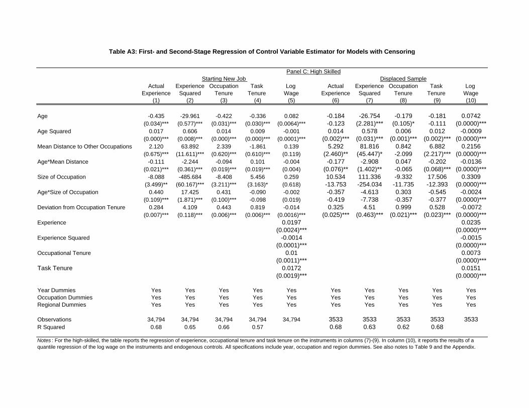
Actual Experience Occupation Task Log Actual Experience Occupation Task Log Experience Squared Tenure Tenure Wage Experience Squared Tenure Tenure Wage

(1) (2) (3) (4) (5) (6) (7) (8) (9) (10)

Age -0.435 -29.961 -0.422 -0.336 0.082 -0.184 -26.754 -0.179 -0.181 0.0742(0.034)*** (0.577)*** (0.031)*** (0.030)*** (0.0064)*** -0.123 (2.281)*** (0.105)* -0.111 (0.0000)***

Age Squared 0.017 0.606 0.014 0.009 -0.001 0.014 0.578 0.006 0.012 -0.0009(0.000)*** (0.008)*** (0.000)*** (0.000)*** (0.0001)*** (0.002)*** (0.031)*** (0.001)*** (0.002)*** (0.0000)***

Mean Distance to Other Occupations 2.120 63.892 2.339 -1.861 0.139 5.292 81.816 0.842 6.882 0.2156(0.675)*** (11.611)*** (0.620)*** (0.610)*** (0.119) (2.460)** (45.447)* -2.099 (2.217)*** (0.0000)***

Age*Mean Distance -0.111 -2.244 -0.094 0.101 -0.004 -0.177 -2.908 0.047 -0.202 -0.0136(0.021)*** (0.361)*** (0.019)*** (0.019)*** (0.004) (0.076)** (1.402)** -0.065 (0.068)*** (0.0000)***

Size of Occupation -8.088 -485.684 -8.408 5.456 0.259 10.534 111.336 -9.332 17.506 0.3309(3.499)** (60.167)*** (3.211)*** (3.163)* (0.618) -13.753 -254.034 -11.735 -12.393 (0.0000)***

Age*Size of Occupation 0.440 17.425 0.431 -0.090 -0.002 -0.357 -4.613 0.303 -0.545 -0.0024(0.109)*** (1.871)*** (0.100)*** -0.098 (0.019) -0.419 -7.738 -0.357 -0.377 (0.0000)***

Deviation from Occupation Tenure 0.284 4.109 0.443 0.819 -0.014 0.325 4.51 0.999 0.528 -0.0072(0.007)*** (0.118)*** (0.006)*** (0.006)*** (0.0016)*** (0.025)*** (0.463)*** (0.021)*** (0.023)*** (0.0000)***

Experience 0.0197 0.0235(0.0024)*** (0.0000)***

Experience Squared -0.0014 -0.0015(0.0001)*** (0.0000)***

Occupational Tenure 0.01 0.0073(0.0011)*** (0.0000)***

Task Tenure 0.0172 0.0151(0.0019)*** (0.0000)***

Year Dummies Yes Yes Yes Yes Yes Yes Yes Yes Yes YesOccupation Dummies Yes Yes Yes Yes Yes Yes Yes Yes Yes YesRegional Dummies Yes Yes Yes Yes Yes Yes Yes Yes Yes Yes

Observations 34,794 34,794 34,794 34,794 34,794 3533 3533 3533 3533 3533R Squared 0.68 0.65 0.66 0.57 0.68 0.63 0.62 0.68

Notes : For the high-skilled, the table reports the regression of experience, occupational tenure and task tenure on the instruments in columns (7)-(9). In column (10), it reports the results of a quantile regression of the log wage on the instruments and endogenous controls. All specifications include year, occupation and region dummies. See also notes to Table 9 and the Appendix.

Table A3: First- and Second-Stage Regression of Control Variable Estimator for Models with Censoring

Starting New Job Displaced SamplePanel C: High Skilled

(1) (2) (3) (4) (1) (2) (3) (4)

Residual Experience -0.031 -0.044 -0.018 -0.019 -0.015 -0.031 -0.01 0.015(0.002)*** (0.009)*** (0.006)*** (0.035) (0.002)*** (0.004)*** (0.002)*** (0.011)

Exp. Res.* Experience 0.003 0.008 0.004 0.005 0.004 0.007 0.003 0.005(0.001)*** (0.001)*** (0.001)*** (0.002)** (0.000)*** (0.001)*** (0.001)*** (0.001)***

Exp. Res.* Experience Squared 0.000 0.000 0.000 0.000 0.000 0.000 0.000 0.000(0.000) (0.005) (0.000) (0.000) (0.000)** (0.000)** 0.000 0.000

Exp. Res.* Task Tenure (0.001)*** -0.004 -0.004 -0.004(0.001)*** (0.002)* (0.001)*** (0.001)***

Exp. Res.* Occupation Tenure -0.001 0.001 -0.001 0.002 -0.002 0.000 -0.002 0.000(0.001) (0.001) (0.001) (0.002) (0.000)*** (0.000) (0.001)*** -0.001

Residual Occupation Tenure 0.066 0.063 0.039 0.041 0.039 0.024 0.032 0.054(0.003)*** (0.006)*** (0.005)*** (0.013)*** (0.001)*** (0.007)*** (0.003)*** (0.009)***

Occ. Res.* Experience -0.004 -0.004 -0.002 -0.002 -0.002 0.000 -0.001 0.001(0.001)*** (0.001)*** (0.001)* (0.002) (0.000)*** (0.000) -0.001 (0.001)

Occ. Res.* Experience Squared 0.000 0.000 0.000 0.000 0.000 0.000 0.000 0.000(0.000)*** (0.000)*** (0.000)** (0.000) (0.000)*** (0.000) (0.000)*** 0.000

Occ. Res.* Task Tenure 0.005 0.004 0.002 0.001(0.001)*** (0.002)** (0.000)*** (0.001)

Occ. Res.* Occupation Tenure -0.002 -0.003 -0.002 -0.003 -0.003 -0.004 -0.004 -0.004(0.000)*** (0.000)*** (0.001)*** (0.001)*** (0.000)*** (0.000)*** (0.000)*** (0.000)***

Residual Task Tenure 0.018 0.000 0.032 -0.05(0.006)*** (0.035) (0.003)*** (0.020)**

Task Res.* Experience -0.003 0.001 -0.003 0.001(0.001)** (0.002) (0.001)*** (0.001)

Task Res.* Experience Squared 0.000 0.000 0.0001 0.000(0.000)*** (0.000) (0.000)*** (0.000)

Task Res.* Task Tenure 0.001 -0.001 0.000 0.000(0.001)* (0.001) (0.001) (0.001)

Task Res.* Occupation Tenure -0.004 -0.004 -0.003 -0.002(0.001)*** (0.002)** (0.000)*** (0.001)**

P value for Joint Significance 0% 0% 0% 0% 0% 0% 0% 0%

Table A4: Impact of Residuals on Wage Equation (Table 9)

Panel A: Low Skilled Panel B: Medium Skilled

Notes : The table reports the coefficients on the residuals and their interaction with the main regressors to control for selection in Table 9. The column number in this table correspond to thecolumn numbers (1) to (4) in Table 9. Standard errors are bootstrapped with 100 replications. The last column reports the p-value of the test for joint significance of the residuals and theinteraction terms. See also notes to Table 9.