how did the paris bourse react to the 1929 nyse krack v1
TRANSCRIPT
How did the Paris Bourse react to the 1929 crash at the NYSE?
Preliminary work
Raphaël Hekimian1 and David Le Bris2
04/25/2014
1 Doctoral student in West Paris University and at the Paris School of Economics 2Associate Professor at Kedge Business School
Abstract: The aim of this paper is to study the reaction of the Paris Bourse on the aftermath of the NYSE crash in late October 1929. We constitute a dataset of daily French stock and state bond prices that we add to the already existing daily series of the Dow Jones on the period from February 1929 to March 1930. We use time series modeling to show that the French stock market is featured by low volatility and pretty high stability during the period, evidencing there was no crash at the Paris Bourse. We observe a reallocation of capital with the French state bonds prices increasing on the same proportion as the stock prices decrease over the period. We also open the discussion on France being a potential safe haven at the aftermath of the New York crash for international investors. Confronting the literature with monetary statistics from the Banque de France, we confirm the effects of a devaluated French Franc in the late 1920s.

Introduction
The recent French economic crisis is part of the global financial crisis that emerged in the United States. Most of the economists quite agree on the fact that the only comparable crisis in international finance history is the Great depression of the 1930s. Indeed, this major event of the 20th century also started in the US before spreading all over the planet. France is one of the more impacted countries by the Great Depression even if it is with a lag compared to the US; the French industrial production of 1937 is 28 % lower than the one observed in 1929 (Landes, 2000 p. 534). But the channel of the propagation of the crisis from US to France is still an open question. The devaluation of the Sterling in July 1931 is frequently observed as the starting point of the Great Depression in France; “Our country which was cheap in 1930 became suddenly expansive in 1931” said Charles Rist (Braudel and Labrousse, 1980, t.4, p. 656). In this paper, we investigate on the short term reaction of the Paris in the six month after the crash of October 1929 at the NYSE, using a new dataset of daily stock prices collected at the archives of the French Ministry of Finance. These daily prices provide a clear demonstration that the contagion of the Great Depression is not the result of a contagion of the stock market crash. Indeed, the French stock market remains stable during the US crash. Using these data, we then measure the higher stability of the French market compared to the US one at that time. This stability is not affected by the US crash. We do observe an influence of the US market on the French one but at a weak level as demonstrated by the very low correlation among the two markets. This stability of the French stock market could be the result of the monetary situation. After the excessive devaluation of the Franc in 1928, France accumulated gold thanks to commercial surplus. These important gold reserves in France could motivate investors to remain invested in French stocks. This attractive characteristic of the French financial market is supported by the rise, after the US crash, of the French state bond. This rise allows the French state bond rate to decrease under the UK one for the first time in history. France as a safe haven after the US crash? After describing the dataset in section 2, we will go back in section 3 to the particular French monetary situation in the late 1920s and the early 1930s, featured by a continuous increase in the accumulation of gold by the French central bank and a clear wish of stability maid by economic authorities. Section 4 presents the econometrical findings of the paper, in particular we show that no crash occurred in Paris in late October 1929, which evidence the absence of propagation of the crisis by the financial channel. Section 5 opens the discussion on the assumption that France may have been a safe haven before investors anticipate the devaluation of the Sterling.
1. Dataset and descriptive analysis
We collected daily spot3 prices for forty individual stocks listed at the official list4 of the Paris Bourse. Those stocks are the forty highest market capitalizations at the beginning of 1929. Our dataset covers the period from February 1929 through the end of March 1930.
We then reconstruct a blue chip weighted index we call CAC 40, for which the daily return is given by:
�����=
∑ ���ℎ ��� × ������ℎ ��������
���
∑ ���ℎ ��� × ������ℎ ������
���
− 1
This index allows us to interpret most of the movements of the French equity market since we know that the aggregated market capitalization of our forty firms represent around 60% of the total market capitalization of the Paris Bourse (Le Bris and Hautcoeur, 2010).A blue chips index does reflect the overall market (Annaertet al., 2011).
We also collected daily prices of the most important French state bond of that time: the “Rente 3% perpetuelle”.It is a government bond issued several times during both the 19thand the20thcentury. It has the particularity not to be depreciable: the government pays a fixed coupon for an undefined period of time. This asset is a very liquid security. The market capitalization of the Rente 3% is around 40 billion francs at the beginning of 1929 (at the same time, the capitalization of our historical stock prices index is around 60 billion).
Finally, we use the Dow Jones Industrial index, which is the only daily stock prices index of the New York Stock Exchange (NYSE) available for our period, despite his well known defaults of being weighted by stock price and not by market capitalization.
3The Paris Stock Exchange had already a term market and an option market but we only collected prices for the
spot market. 4 There were already an OTC market inside the Paris Bourse, but all the data we collected only concerns the
official market.

Graph 1 : co-movements of Dow Jones, CAC 40 and the Rente 3% (base 100 in September1929)
Source: Authors for CAC and Rente 3%, Federal Reserve of Saint Louis for DJ
As we can see in the Graph 1, not any shock occurred on the French stock market after the crash at the NYSE. It is a huge surprise to observe that even the worst days in the NYSE seems free of any impact in the Paris market; 1929 October 28, the Dow Jones fall by 13.47 % but our French index decreased by 0.60 % and 2.99 % the day after when the Dow Jones suffered another fall of 11.73%. After these two days, the loss is 23 in New-York and only 5 % in Paris. This absence of any contagion of the US crash is really different from what was observed during the last financial crisis.
Moreover, the correlation coefficient between French and American stock returns are almost null before September 1929, and stay very low after, around 0,15 (without taking into account the volatility, which would certainly even lower this figure in a crisis period like this one). On the other hand, we can see that the price of our safe asset (Rente 3%) increases for about 20 percentage points, whereas the French Stock prices index decrease from about 20 percentage points.
This makes us think that there could have been a sort of flight to quality for investors, using the Paris Bourse as a safe haven during the period after the crash of October 1929.
When researchers in history of finance study the Paris Bourse, a prominent feature is the lack of an important data to analyze the market behavior: the volume of traded securities. We tried to solve this issue by collecting two series that we take as proxies for the volumes: the tax on financial transactions and the amount of compensations in between the brokers. Both series have several limits that we discuss below.
40
50
60
70
80
90
100
110
120
130
DJ
CAC
Rente 3%

The tax on financial transactions is available on bi-weekly basis. The tax levies a fixed rate on the total volume traded at the Paris Bourse for securities listed on the official list, for both the spot and the term market. Since we only have spot prices, there is an upward bias that is difficult to estimate if we want to link our prices with this volume proxy. We can suppose this bias constant overtime. Moreover, there is a frequency issue because the prices are daily and the tax is only available every two weeks. Graph 2 exhibits this series:
Graph 2: Bi-weekly amount of taxes raisedin million Francs
Source: Authors
Our other proxy for the volume traded is the daily amount of compensations between brokers operating on the official market. Here the frequency is the same as for our prices and moreover, it only concerns the spot market. Nevertheless there is another bias, once again very hard to estimate. When a broker executes an order for a client, another broker has to compensate for the amount of the transaction, by an order of his own clients that goes on the opposite way. But if a broker has already two clients giving him opposite orders, he can compensate by himself and then doesn’t have to ask a colleague. In this case, the compensation is not reported in the brokers company’s balance sheet5. This also constitutes a downward bias but we can also suppose it constant over time. Graph 3 illustrates this series:
5 Until 1987, a brokers company called “Compagnie des Agents de Change” had the monopoly on all the
transactions at the Paris Bourse, but the institution had to remain accountable by the Sate.
0
5
10
15
20
25
30

Graph 3: Daily compensations in million Francs
Source: Authors
2. The monetary situation
The French monetary policy during the interwar period and especially during the 1920’s has been well studied. When WW1 started in 1914, France, along with Great Britain, abandoned the Gold Standard to follow expansionary monetary policies in order to finance the war effort. According to Blancheton (2000), France financed the war mostly by issuing debt (74%), the rest by raising taxes (15%) and with the advances of the Banque de France (11%). The situation of public finance did not recover after the war because the FrenchTreasury(MouvementGénéral des Fonds,) anticipated that Germany would pay for war damages as France paid Germany after the Franco-Prussian war in 1871.
At that time, both the central bank and the Treasury still thought it was manageable to restore the pre-war parity of the franc. They tried to stick to a deflationary monetary policy, by containing the circulation of money under a certain ceiling. Once they finally figured out Germany would never be able to pay the entire amount of the reparations, Blancheton shows that the Treasury faced his obligations by using indirect advances of the Banque de France(via commercial banks), which increased the circulation and led to speculative attacks against the franc in the 1925-26.
Even if Hautcoeur and Bordo (2007) showed that stabilization was historically possible since 1924, the circulation kept growing thanks to fraudulent accounting writings by the central bank that led to the “fake balance sheets scandal”. Finally, when the depreciation of the Franc reached his top in July 1926, Raymond Poincare returned to the Government and restored confidence. The franc/sterling parity decreased until the central bank stabilized de factothe
-
20,00
40,00
60,00
80,00
100,00
120,00

Franc by intervening directly on the foreign exchange market. The law of June 1928 ratifies the return to the Gold Standard, but with a devaluation of four fifth of its prewar parity.
This devaluation of the Franc was probably excessive providing to the French economy an artificial competitivity especially compared to the UK which return to the pre-war parity. This competivity leads France to accumulate commercial surplus paid in gold. Thus, France accumulates gold since 1928. Irwin (2012), as other before him (see Eichengreen, 1990) highlights the bad consequences of this French accumulation of gold. If gold is accumulated by a central bank that is not willing to expand its monetary base, it creates a deflationary bias for the rest of the world. The author blame the monetary policy of the Banque de France, along with the Federal Reserve, for letting gold reserve being accumulated without monetizing them. Over the period we are interested in, Mouré (1998) uses the 1929 annual report of the central bank to cite the governor Emile Moreau justifying those gold inflows. Moreau explains that the main reason of this gold movement is due to the decrease in the interest rates in London and New-York. Moreau rejects any assumptions of direct interventions from the central bank.
Irwin, using Mouré’s monthly data of French gold reserve and cover ratios, shows that by increasing the cover ratio on a same scale as the gold reserves, the monetary base stays stable. According to Irwin, this is how the central bank “neutralized” the gold inflows. In fact, they could not properly sterilized the gold inflows by operating open market operations like the Fed did (Friedman and Schwartz 1963) because of the monetary law of June 1928 that forbids both open market operations and interventions on the foreign exchange market. The combination of those two restrictions leaves nothing but the cover ratio as a monetary tool to manage for the amount of francs in circulation.
In order to verify if this result is true over our period, we use bi-monthly data of gold reserve and total circulation of francs.6The data are computed in indexes (base 100 at the beginning of our period) so we can compare the evolution of each series, see Graph 4 below:
6 Data available online, based on the bi-monthly balance sheet (Situation hebdomadaire) of the Banque de
France.

Graph 4: Co-evolution of the Gold reserves and the amount of Francs in circulation
Source :Banque de France
We can see that while the gold reserves are increasing from more than 20%, the amount of francs in circulation seems to remain quite stable. Consistently, the cover ratio goes from 41.5% to almost 50% over the period, which confirms the results of Irwin. According to the Monetary Law of 1928, the ratio should be at a minimum of 35 percent, although the Bank wanted a minimum of 40 percent in practice. This is about where the cover ratio was in December 1928. Of course, this was a mandatory lower bound and there was no maximum cover ratio beyond which the Bank was forbidden to go. By 1930, the Bank of France cover ratio rose to over 50 percent. In January 1931 it reached 55 percent; at this point the Bank of France considered but rejected a proposal to suspend its gold purchases (Mouré 2002, 188). By 1932, the cover ratio had risen to the amazing level of nearly 80 percent!
We also looked at the bi-weekly reports of the board of governors of the Banque de France over the period and found some interesting statements. Indeed, Emile Moreau explicitly warns off against the monetary circulation movements in early 19307 and especially in terms of gold inflows coming from abroad. In May 1930, he even plans on decreasing the discount rate after the Bank of England decreased its own, in order not to see more gold inflowing.
In this section we outlined the solidity of the French monetary context where a stabilized currency is backed with increasing reserves of gold. We find that this monetary situation is likely to constitute a safe environment for investors looking for stable financial assets.
7 See bi-weekly report of the Banque de France from 1930/01/02; 1930/01/23; 1930/01/30; 1930/02/20;
1930/03/20.
70
80
90
100
110
120
130
31
/01
/19
29
03
/03
/19
29
03
/04
/19
29
03
/05
/19
29
03
/06
/19
29
03
/07
/19
29
03
/08
/19
29
03
/09
/19
29
03
/10
/19
29
03
/11
/19
29
03
/12
/19
29
03
/01
/19
30
03
/02
/19
30
03
/03
/19
30
03
/04
/19
30
Circulation
Gold reserve

In the next section, we will look forward to test the stability of the Paris Stock Exchange to see if it corroborates this argument.
3. The absence of any crash in France in 1929
In this subsection we use our daily series of French and American stock prices to look for differences in term of risk. We will try toemphasizetheir differences, especially in terms of the volatility structure for each market since volatility is the common proxy for risk.
In order to find out if our two series in raw data have a trend, we first proceed to unit root tests on the series turned into logarithms. Results show that the two series are integrated at the first order, which mean that we have to differentiate them to avoid from stationarity issues. Thus, westudy the returns of the historical CAC 40 (�����
) and those of the Dow Jones (����
). We will first study the returns separately in order to outline some interesting different features among the two series, using ARMA and GARCH specifications. Then we will try to characterize their relationship by testing for causality, analyzing the correlations and estimate a vector autoregressive model.
3.1.The French stock returns
A first look on the descriptive statistics of ����� gives us some intuitions:
The Skewness coefficient � =– 0,3(≠ 0)shows us that the asymmetry in the distribution is not very strong. A Skewness below zero means that a negative shock has a little more impact than a positive shock. The Kurtosis coefficient ( = 4,2(> 3) outlines a little Kurtosis excess which denote that there is a little higher probability of extreme event to occur.
Of course, we don’t expect an equity return to follow a Gaussian law and the Jacque-Bera test clearly rejects this hypothesis but nevertheless, it still seems quite reasonable to estimate a linear model to compute this series.
Another intuition that corroborate this idea is given by the graph of �����:

The volatility of the returns does not seem to have a particular structure: the high volatilities are not clearly followed by other high volatilities and it is the same for low volatilities. It is then legitimate to use linear specifications.
We use the Box and Jenkins (1970) methodology in order to specify the best ARMA process to model �����
. We end up estimating an autoregressive process at the order 1 (AR(1)):
�����= ,� + .������/0
+ ε� (1)
Variable Coefficient Std. Error t-Statistic Prob.
,� -0.000512 0.000636 -0.805076 0.4214
.� -0.229944 0.055550 -4.139431 0.0000
The estimation output shows that the estimated .� is significant. Moreover, after testing for the absence of autocorrelation and homoscedasticity8 on the residuals, we find that ε�follow a white noise. It is important to notice that we do not detect any ARCH effect, which is usually the case for equity returns especially at a daily frequency).This feature allows us to test for the stability of the parameters.
8 We used a Ljung-Box test based on the correlogram of the residuals to detect the presence of autocorrelation
and an ARCH test for the homoscedasticity.
-.08
-.06
-.04
-.02
.00
.02
.04
.06
.08
1929Q1 1929Q2 1929Q3 1929Q4 1930Q1
Volatility of French stock returns

Indeed, since there are no issues on the residuals, we are able to apply a basic Chow test by estimating the model (1) in two sub-samples, before and after the crash at the NYSE in late October 1929.
Chow Breakpoint Test: 10/28/1929 Null Hypothesis: No breaks at specified breakpoints
Equation Sample: 2/05/1929 3/31/1930
F-statistic 2.632899 Prob. F(2,296) 0.0736
Log likelihood ratio 5.290041 Prob. Chi-Square(2) 0.0710
Wald Statistic 5.264331 Prob. Chi-Square(2) 0.0719
The p-value of the test Prob. F(2,296) = 0,0736 > 0,05: the null hypothesis is rejected. The parameters are stable before and after the crash.
3.2.The American stock returns
Following the same empirical strategy, we first focus on the graph and the descriptive statistics of ����
.
-.16
-.12
-.08
-.04
.00
.04
.08
.12
1929Q1 1929Q2 1929Q3 1929Q4 1930Q1
Volatility of the American stock returns

Unlike�����, it seems that we are able to graphically identify clusters in volatility: the high
strong variations are followed by other strong variations while small variations are followed by other small variations.
Comparing the descriptive statistics with the previous ones, we can see that for ����: ( =
−15,1 ≫ 3 denotes a strong probability of extreme events to occur while � = −1,5 is quite an indication in favors of nonlinearity. It says that negative shocks have more impact than positive shocks: the volatility is higher after a decrease in the returns than after an increase.
We use the same methodology to model ���� and end up with the following AR(3):
����= ,� + .�����/0
+ .5����/6+ .7����/8
+ ε� (2)
Variable Coefficient Std. Error t-Statistic Prob.
,� -0.000390 0.001351 -0.288762 0.7730
.� 0.216975 0.056426 3.845289 0.0001
.5 -0.386336 0.053239 -7.256616 0.0000
.7 0.253402 0.056443 4.489501 0.0000
We can see that all estimated .� are significant. On the other side, the residuals ε� are tested to look for heteroscedasticity. After running an ARCH test, we find that there is an ARCH effect on the estimated ε�, meaning that there is a conditional heteroscedasticity in the residuals. In this case we have to add a conditional variance equation to our model to take into account the nonlinearity of the residuals. This leads to a GARCH specification, but after several estimations9 using the maximum-likelihood method, we end up finding that the best way to model ����
is to use a TGARCH (Zakoian 1990) specification. So we add to the mean
equation (2) the TGARCH (Threshold GARCH) equation of the conditional variance:
9� = ,� + ,��:�;�
� − ,�;:�;�
; + .9�;� (3)
With :�;�� = < =(>, ε�;�) �?:�;�
; = <��(>, ε�;�)
The estimation on both equation (2) and (3) gives us the following results:
9 We estimated several GARCH process but none of them respected the positivity constraints on the coefficient
imposed by the quadratic specification of GARCH models.We then used EGARCH and TGARCH process to avoid
those constraints, we then choose between them via information criteria optimization.

Mean Equation (2)
Variable Coefficient Std. Error z-Statistic Prob.
,� -0.000348 0.000798 -0.436554 0.6624
.� 0.110883 0.058744 1.887580 0.0591
.5 -0.012831 0.027470 -0.467113 0.6404
.7 0.190656 0.035069 5.436671 0.0000
Variance Equation (3)
,� 1.92E-05 3.57E-06 5.377544 0.0000
,�� -0.192487 0.020860 -9.227495 0.0000
,�; 0.583477 0.077645 7.514689 0.0000
.) 0.817269 0.030555 26.74706 0.0000
Although some coefficients of the mean equation are not anymore significant, we can see that all the coefficients of the variance equation are significant, which means that there is
information contented in the volatility of ����10. In fact, ,�
� and ,�;have opposite sign, which
evidence the phenomenon of asymmetry.
What can we learn from those separate analyses of our stock returns? In this subsection we emphasized very different features in the volatility structure of the two stock markets. By using time series modeling, we showed that the returns on French stocks can be easily computed by linear models while the returns on American stocks have to be computed with nonlinear models. Yet the nonlinear models have been developed in order to face economic stylized facts such as the asymmetry phenomenon or the persistence of shocks due to financial crisis. Those facts have been widely observed on a lot of recent financial series on the period from 1973 and the fall of the Bretton-Woods monetary regime, until today. This period is known to be very unstable regarding financial markets, with numerous financial crisis and asymmetric structure in asset’s volatility.
We take this result as quite an indication of the strength of the French stock market, which appears to look more stable and less risky comparing to the American one. The Chow test confirms this view.
10
We would not use this model to make any predictions knowing there are insignificant coefficients of the
mean equation. Still, the purpose here is to find evidence of the nonlinearity of ����.

3.3.The relationship between American and French stock returns
The correlation among stock markets is a well-known issue. Goetzmann and al. (2005)
highlight the instability of the international correlations. The US market is viewed as a leader
one since the 1920s.
First we test for Ganger causality between �����and ����
:
Pairwise Granger Causality Tests NullHypothesis: Obs F-Statistic Prob. �����
does not Granger Cause ���� 299 0.73377 0.4810
���� does not Granger Cause �����
16.7355 1.E-07
The test clearly rejects the null hypothesis of ���� not causing �����
, so the returns on the
Dow Jones affect those of the CAC, but the opposite is not verified, so there are no feedback effects. This result confirms that on one hand, the relationship between the returns deserves a further investigation and on the other hand, that what happened at the NYSE around the shock of 1929 has influenced the movements in Paris.
We can now try to model the relationship with ����� as the dependent variable,regarding the
results of the Granger test. Using the VAR (Vector AutoRegressive) specification, we estimate the following relationship11:
�����= ��������/0
+ �5�����/6�7�����/8
+ ������/0+ �5����/6
+ �7����/8+ ε� (4)
Variable Coefficient Std. Error t-Statistic
� -0.00063 0.00075 -0.85215
�� -0.22684 0.05849 -3.87780
�5 -0.01431 0.05987 -0.23901
�7 -0.07495 0.05562 -1.34752
�� 0.18371 0.03403 5.39689
�5 -0.00735 0.03414 -0.21525
�7 0.01094 0.03548 0.30837
11
To select the right p-order of the VAR(p), we estimated eight VAR process for p=1,…,8 and we chose p=3
because it minimized the information criteria.

The estimation output above shows us that ��, �7, �� and �7 are significant. We could expect it for ��and �7because we already showed that �����
depended on its own lagged values in a
univariate specification (see section 4.1.1.). But �� and �7being significantis an evidence that the lagged values of ����
contain information on�����which means that we are able to explain
some of the movements in Paris with what happened in New York within the last three working days.
Nevertheless, if we look at the correlations between ����� and ����
over the whole sample,
the Pearson correlation coefficient is equal to 0,08. If we divide the sample in two sub-periods (before and after October 1920), the number goes from 0 to 0,15 after the crash. Those low figures don’t encourage investigating on an hypothetical contagion between the two stock markets. Indeed the increase in correlations is already low, but if we correct from heteroscedasticity (Forbes and Rigobon 2000), we would have even lower figures, which allows us not to test for contagion phenomena.
4. France as a safe haven?
In the last two sections, we highlighted the strength of the French Franc and the quite stability of the Paris Bourse over the period framing the crash of October 1929 in New-York. In this section we will open the discussion on whether or not it is possible to characterize France as a safe haven for investors.A first intuition is given by the Graph of the interest rates spread between UK and France:

Source: UK Consol from Sylla’s website and Rente 3 % from authors.
We can see that, apart from WWI, the French rates go under the UK’s around 1928. For the first time, the French state paid a lower rate than the UK. This figure could be the result of the expectation of the devaluation of the sterling. The investors are not attracted to invest in sterling if this currency suffers the risk to be devaluated. This risk is priced by a higher rate. Contrarily, the french Franc, which is undervalued since 1928, does not suffer this risk. So during our period, the Franc seems to be a safe currency for investors.
Then, the first insight we need to check for is the presence of international capital movements in direction of France. Aldcroft (1977) uses the following table to describe the international lending around 1929:
Net Capital Movements of Creditor Countries, 1927-1931 ($ millions)
Year France Netherlands Sweden Switzerland U.K. U.S.A. Total
1927 -504 -95 -65 -92 -385 -829 -1 970
1928 -236 -73 -19 -94 -569 -1 250 -2 241
1929 +20 -75 -71 -86 -574 -628 -1 414
1930 +257 -66 -26 -36 -112 -380 -363
1931 +791 +259 +22 +369 +313 -330 +1 424
Source: Mikesell (1962)
-2,00%
-1,50%
-1,00%
-0,50%
0,00%
0,50%
1,00%
1,50%
2,00%
2,50%
3,00%
18
50
18
53
18
56
18
59
18
62
18
65
18
68
18
71
18
74
18
77
18
80
18
83
18
87
18
90
18
93
18
96
18
99
19
02
19
05
19
08
19
11
19
14
19
17
19
20
19
24
19
27
19
30
19
33
19
36
19
39
19
42
19
45
19
48
Spread UK-France
We can observe that France is the first of those historically creditor countries to become net capital importer in 1929. The yearly frequency of those data does not allow us to make any conclusion, but it seems to indicate that it is either that French capital was repatriated, or that foreign capital inflows came into France (or a combination of the two).
Another indication of capital inflows can be found in the archives of “Le Temps”12, a serious and widespread daily French newspaper at the time(the ancestor of the newspaper Le Monde). We looked at the Bulletin Financier (i.e. the financial part of the newspaper) the first days after the crash and found some interesting information. For example, on the edition of October the 28th we can read: “European capitals that were placed in New-York so far, where neither the stock market performances nor the daily interest rate of the money market are longer attractive, begin to be massively repatriated, including French capitals which will only reinforce our money market”. On October the 30th: “the weakness of yesterday’s performances must firstly be attributing to foreign sells, determined by the bad performances of foreign financial places such as the Amsterdam Bourse”. Of course, those quotes are not satisfying but it might be interesting to dig deeper by exploring other newspapers.
In addition, we can find several times in Le Temps that the Rentes (i.e. the French State bonds) are resisting to the general decrease of the market13. The data on prices of the Rente 3% we collected confirm this insight; since we can see its price growing about 20 percentage points from September 1929 to the end of March 1930 (see Graph 1).
This leads us to another assumption: if on one hand the state bond prices increase from about 20% while stock prices decrease from 20%, and on the other hand the amount of Francs in circulation is stable, we may think that investors proceeded to an assets reallocation on their portfolio in favor of the Rente 3%. This would evidence a sort of flight to quality phenomenon. Such phenomena should be empirically supportable within a CAPM framework (Vayanos, 2004) or by estimating specific GARCH process (Cappiello, Engle and Shepard, 2006). But first we would have to assume that the Rente 3% is a liquid and risk free asset.
Another argument makes pertinent the use of the Rente 3%. The asset has to be a good proxy of the state bonds market. Indeed, his market capitalization is significant (see section 2). Moreover, it is important to notice that it is one of the only listed state bonds that have not been issued during or after WWI. Indeed, as we said in section 3, most of the war effort had been financed by issuing short term debt. In 1926, the Caisse Autonome d’amortissement (CAA) is created by public authorities in order to protect the Treasury from the liquidity risk linked to all those short term debt issued during the war. The CAA’s mission was to convert short term debt into long term debt. After this mission succeeded, it started to intervene on the Rentes market in 1928-1929 (Ducros, 2010). According to Toytot (1991), the CAA used his technical skills in debt conversion on the Rentes issued between 1920 and 1928, which does not concern our Rente 3%. Such interventionsof debt repurchasing are able to create an
12
Available online at:
http://gallica.bnf.fr/ark:/12148/cb34431794k/date1929.r=Le%20Temps%20quotidien.langFR 13
Seeeditions of 10/30/1929 ; 10/31/1929 ; 11/01/1929
upward bias in the price which would cause troubles in the interpretation of estimated coefficients.
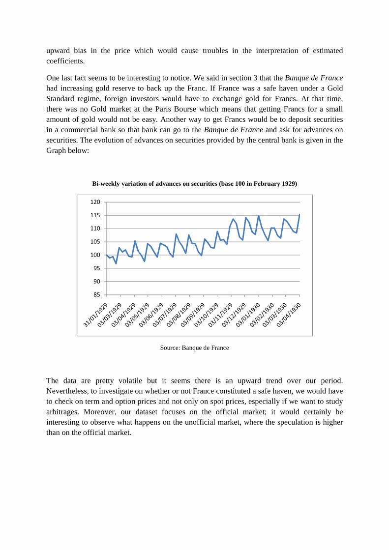
One last fact seems to be interesting to notice. We said in section 3 that the Banque de France had increasing gold reserve to back up the Franc. If France was a safe haven under a Gold Standard regime, foreign investors would have to exchange gold for Francs. At that time, there was no Gold market at the Paris Bourse which means that getting Francs for a small amount of gold would not be easy. Another way to get Francs would be to deposit securities in a commercial bank so that bank can go to the Banque de France and ask for advances on securities. The evolution of advances on securities provided by the central bank is given in the Graph below:
Bi-weekly variation of advances on securities (base 100 in February 1929)
Source: Banque de France
The data are pretty volatile but it seems there is an upward trend over our period. Nevertheless, to investigate on whether or not France constituted a safe haven, we would have to check on term and option prices and not only on spot prices, especially if we want to study arbitrages. Moreover, our dataset focuses on the official market; it would certainly be interesting to observe what happens on the unofficial market, where the speculation is higher than on the official market.
85
90
95
100
105
110
115
120

References:
Aldcroft D. H. (1977), From Versailles to Wall Street 1919-1929, p. 262, University of California Press
Annaert and al. (2011), « Are blue chip stock market indices good proxies for all-shares market indices? The case of the Brussels Stock Exchange 1833-2005 », Financial HistoryReview
Blancheton B.(2000), Le Pape et l’Empereur, la Banque de France, la direction du Trésor et la politique monétaire de la France (1914-1928), Paris, Albin Michel
Braudel F. and Labrousse E (1980), Histoire économique et sociale de la France, Paris, PUF.
Cappiello L., Engle R. F. and Sheppard (2006), « Asymetric Dynamics in the Correlations of Global Equity and Bond Returns », Journal of Financial Econometrics.
Ducros J.(2010), « Du fardeau à la modernisation économique et financière. L’endettement en France, 1926-1929.», Master Thesis.
Eichengreen B.,(1990), Elusive Stability: Essays in the History of International Finance, 1919–1939, New York: Cambridge University Press.
Forbes K. and Rigobon R. (2000), « Measuring Contagion : Conceptual and Empirical Issues », NBER.
Friedman, M. and Anna J. Schwartz. (1963). A Monetary History of the United States,
1867–1960. Princeton, NJ: Princeton University Press.
Hautcoeur P. C. &Bordo M. D. (2007), « Why didn’t France follow the British stabilization after World War I? », European Review of Economic History, Cambridge University Press.
Irwin D. A. (2012), « The French Gold Sink and the Great Deflation of 1929-32 », Cato Papers on Public Policy, Vol. 2
Landes D. (2000), L’Europe technicienne, Paris, Gallimard.
Le Bris D. and Hautcoeur P. C.(2010), « A challenge to triumphant optimists? A blue chips index for the Paris stock exchange, 1854-2007 », Financial History Review
Mouré K.(1998), La politique du franc Poincaré, Paris, Albin Michel
Mouré K.(2002), The Gold Standard Illusion: France, the Bank of France, and the International Gold Standard, 1914–1939 . New York: Oxford UniversityPress
Sauvy A. (1984), Histoire économique de la France entre les deux guerres Volume 3,Paris, Economica
Toytot A. (1991), «La Caisse autonome d'amortissement : une expérience de gestion de la dette publique (1926-1932) », Revue d'économie financière. Hors-série.
Vayanos D.(2004), « Flight to quality, flight to liquidity, and the pricing of risk » Working paper MIT.