how an earnings supplement can affect the marital behaviour of

How an Earnings Supplement Can Affectthe Marital Behaviour of Welfare Recipients:Evidence From the Self-Sufficiency Project

Kristen HarknettPrinceton University

Manpower Demonstration Research Corporation

and

Lisa A. GennetianManpower Demonstration Research Corporation

SOCIAL RESEARCH and DEMONSTRATION CORPORATION

The Self-Sufficiency Project is sponsored by Human Resources Development Canada.

The Social Research and Demonstration Corporation is a non-profit organization and registered charity with offices inOttawa, Vancouver, and Sydney, Nova Scotia. SRDC was created specifically to develop, field test, and rigorouslyevaluate social programs designed to improve the well-being of all Canadians, with a special concern for the effects ondisadvantaged Canadians. Its mission is to provide policy-makers and practitioners with reliable evidence about whatdoes and does not work from the perspectives of government budgets, program participants, and society as a whole.As an intermediary organization, SRDC attempts to bridge the worlds of academic researchers, government policy-makers, and on-the-ground program operators. Providing a vehicle for the development and management of complexdemonstration projects, SRDC seeks to work in close partnership with provinces, the federal government, localprograms, and private philanthropies.

Copyright © 2001 by the Social Research and Demonstration Corporation

iii

Table of Contents

Tables and Figures . . . . . . . . . . . . . . . . . . . . . . . . . . . . . . . . . . . . . . . . . . . . . . . . . . . . . . . . . . . . . iv

Acknowledgements . . . . . . . . . . . . . . . . . . . . . . . . . . . . . . . . . . . . . . . . . . . . . . . . . . . . . . . . . . . . . v

Abstract . . . . . . . . . . . . . . . . . . . . . . . . . . . . . . . . . . . . . . . . . . . . . . . . . . . . . . . . . . . . . . . . . . . . vii

Introduction . . . . . . . . . . . . . . . . . . . . . . . . . . . . . . . . . . . . . . . . . . . . . . . . . . . . . . . . . . . . . . . . . . 1

Prior Research . . . . . . . . . . . . . . . . . . . . . . . . . . . . . . . . . . . . . . . . . . . . . . . . . . . . . . . . . . . . . . . . 3

The SSP Model and Evaluation . . . . . . . . . . . . . . . . . . . . . . . . . . . . . . . . . . . . . . . . . . . . . . . . . . . 7

Conceptual Framework . . . . . . . . . . . . . . . . . . . . . . . . . . . . . . . . . . . . . . . . . . . . . . . . . . . . . . . . . . 9

Data and Variables . . . . . . . . . . . . . . . . . . . . . . . . . . . . . . . . . . . . . . . . . . . . . . . . . . . . . . . . . . . . 13

Empirical Analysis . . . . . . . . . . . . . . . . . . . . . . . . . . . . . . . . . . . . . . . . . . . . . . . . . . . . . . . . . . . . 17

Empirical Results . . . . . . . . . . . . . . . . . . . . . . . . . . . . . . . . . . . . . . . . . . . . . . . . . . . . . . . . . . . . . 19SSP�s effect on marriage . . . . . . . . . . . . . . . . . . . . . . . . . . . . . . . . . . . . . . . . . . . . . . . . . . . . 19Mechanisms by which SSP affected marriage . . . . . . . . . . . . . . . . . . . . . . . . . . . . . . . . . . . . . 24Why did SSP�s effect on marriage differ by province? . . . . . . . . . . . . . . . . . . . . . . . . . . . . . . 27

Discussion and Conclusion . . . . . . . . . . . . . . . . . . . . . . . . . . . . . . . . . . . . . . . . . . . . . . . . . . . . . . 33

Appendix A: Key Features of the SSP Earnings Supplement and the SSP Plus Intervention . . . 35

Appendix B: Selected Baseline Characteristics of SSP 36-Month Survey Respondents,by Research Group and Province . . . . . . . . . . . . . . . . . . . . . . . . . . . . . . . . . . . . . . . . . . . . . . 37

Appendix C: SSP Effects on the Risk of Marriage . . . . . . . . . . . . . . . . . . . . . . . . . . . . . . . . . . . 39

References . . . . . . . . . . . . . . . . . . . . . . . . . . . . . . . . . . . . . . . . . . . . . . . . . . . . . . . . . . . . . . . . . . . 41

iv

Tables and Figures

Tables

1: Selected Baseline Characteristics of SSP 36-Month Survey Respondents, by Province . . . . . . 14

2a: SSP Impacts on Marriage and Common-Law Unions Over Three Years of Follow-Up . . . . . 20

2b: SSP Plus Impacts on Marriage and Common-Law Unions Over Three Years of Follow-Up . 21

3: SSP Impacts on Marriage Rates, by Subgroup and Province:Percentage Ever Married or Common-Law, Months 1-36 . . . . . . . . . . . . . . . . . . . . . . . . . . . . 25

4: SSP Impacts on Employment Over 36 Months, by Subgroup and Province:Average Monthly Percentage Employed Full Time . . . . . . . . . . . . . . . . . . . . . . . . . . . . . . . . . 28

5: SSP Impacts on Income, by Subgroup and Province: Average Total Income,Months 1-36, in Dollars . . . . . . . . . . . . . . . . . . . . . . . . . . . . . . . . . . . . . . . . . . . . . . . . . . . . . . 29

6: Selected Characteristics of the Population Residing in the Areas Served by SSP . . . . . . . . . . 31

B: Selected Baseline Characteristics of SSP 36-Month Survey Respondents,by Research Group and Province . . . . . . . . . . . . . . . . . . . . . . . . . . . . . . . . . . . . . . . . . . . . . . 37

C: SSP Effects on the Risk of Marriage . . . . . . . . . . . . . . . . . . . . . . . . . . . . . . . . . . . . . . . . . . . . 39

Figures

1: Monthly Full-Time Employment Rate, by Research Group in Both Provinces Combined . . . . 8

2: Average Monthly Earnings, by Research Group in Both Provinces Combined . . . . . . . . . . . . . 8

3: Intervening Mechanisms . . . . . . . . . . . . . . . . . . . . . . . . . . . . . . . . . . . . . . . . . . . . . . . . . . . . . 10

4: Percentage Married or Common-Law, by Research Group in Both Provinces Combined . . . 19

5: Percentage Married or Common-Law, by Research Group in British Columbia . . . . . . . . . . . 22

6: Percentage Married or Common-Law, by Research Group in New Brunswick . . . . . . . . . . . . 22

7: Percentage Married or Common-Law, by Research Group in New BrunswickSSP Plus Study . . . . . . . . . . . . . . . . . . . . . . . . . . . . . . . . . . . . . . . . . . . . . . . . . . . . . . . . . . . . . 23

v

Acknowledgements

Many thanks to the Manpower Demonstration Research Corporation (MDRC) and the SocialResearch and Demonstration Corporation (SRDC) for access to and use of the Self-SufficiencyProject data, and to Wendy Bancroft, Gordon Berlin, Sheila Currie, John Greenwood, SaraMcLanahan, Charles Michalopoulos, H. Elizabeth Peters, David Ribar, Saul Schwartz, and MartaTienda for helpful discussions and comments.

The Authors

vii

Abstract

Because welfare policies have long been accused of contributing to the breakdown of the nuclearfamily, policy-makers have had an interest in ensuring that welfare and employment policies, at aminimum, do not discourage marriage or encourage marital breakups. Using data from theexperimental evaluation of the Self-Sufficiency Project (SSP), this paper examines the effect of analternative to the mainstream cash welfare system, an alternative that is contingent on work andremoves the usual welfare marriage disincentive on marital behaviour among single-parent welfarerecipients. The effect of such a program on marital behaviour predicted by theory is ambiguous.Eliminating the welfare marriage disincentive should positively affect marriage, but increasingemployment and income, as SSP did, may have either positive or negative effects on marriage. Onaverage, SSP had no effect on marriage. Rather, SSP had opposing effects on marriage across twoprovinces � an increase in marriage in one province and a decrease in marriage in anotherprovince. The opposite direction of the effect in the two provinces cannot be explained bydifferences in the income or employment effects caused by SSP, by differences in sample members�observed characteristics, or by differences in characteristics of the marriage market between thetwo provinces. Our results suggest that unobserved differences in provincial characteristics, such ascultural or marital norms, mediated how SSP affected marriage. These results are consistent withthe empirical literature that finds that local or state fixed effects play an important role inunderstanding the effects of welfare on the incidence and spells of single parenthood in Canadaand the US.

1

Introduction

Welfare policies have long been accused of contributing to the breakdown of the nuclear family.Welfare is commonly blamed for discouraging marriage and encouraging divorce by providing analternative means of financial support for poor mothers and their children.1 Though prior researchon the effects of different sets of welfare policies on family structure is inconclusive, theformation and stability of marriage, particularly among low-income families, has been a long-standing goal of public policy. Yet, marriage disincentives are inherent in the means-tested welfareprograms of Canada and the US (Moffitt, 1992). Under means-tested programs, the added incomecontributed by a spouse will typically make a family ineligible for welfare or reduce its grant amount.

This study utilizes a random assignment design to examine the effect of a generous earningssupplement program with no marriage disincentive on the marital behaviour of welfare recipients.2The Self-Sufficiency Project (SSP) tests a unique approach that eliminates the �traditional�marriage disincentive for welfare recipients by disregarding the income of a spouse or partnerwhen determining eligibility for SSP�s earnings supplement and its amount. Although this policychange should be expected to increase the probability of marriage among welfare recipients, itsexpected effect must be balanced with SSP�s effects on increasing income and full-time employment,both of which have a theoretically ambiguous effect on marital behaviour. Prior empirical worksuggests a relation between local and geographic context, and the effect of income transferprograms on marital behaviour. This paper additionally exploits the provincial variation in the SSPdata � often not found in experimental studies � to examine the extent to which local or geographiccontext versus SSP�s effects on income and employment mediates the effect of SSP on marriage.

There are a number of reasons why it is important to understand the impact of alternative welfareor antipoverty policies, such as those tested in SSP, on marriage. First, empirical evidence suggeststhat children in one-parent families are disadvantaged on a broad array of outcomes comparedwith those in two-parent families (McLanahan & Sandefur, 1994). Part of this difference resultsfrom greater poverty among one-parent families. Thus, children may benefit from policies thatdually increase a family�s self-sufficiency by increasing employment and earnings, and the likelihoodof marriage.3 Second, policies that facilitate a desired marriage or enhance marital stability may alsofacilitate long-term independence from public assistance. Remarriage is the most common route torecovery from the decline in standard of living that women and children face after divorce (Holden& Smock, 1991) and is also a common route off of welfare (Bane & Ellwood, 1994; Moffitt,1992). Third, welfare systems in Canada and the US are currently undergoing major scrutiny andreform. Results from the SSP experiment � as an example of an effective antipoverty program �

1Because the vast majority of the welfare population, including the sample analyzed in this paper, are female, the terms�mothers,� �women,� and the female pronoun are used throughout this paper.

2Here and throughout the text of this paper marriage is broadly construed as legal marriage or common-law marriage.As is explained in further detail later, common-law marriages in Canada entail similar rights and responsibilities tolegal marriages, and are treated similarly by the income assistance system.

3Empirical evidence has suggested that marriage to someone unrelated to the child does not improve the outcomes ofchildren formerly living with a single parent (McLanahan & Sandefur, 1994). However, it is possible that SSP couldincrease marriage between biological parents, which may be beneficial for children. See Morris and Michalopoulos(2000) for a discussion of the effects of SSP on child outcomes.

can help to inform the design of future policies that are targeted to low-income families and thatmay influence marital behaviour. Policy-makers have an interest in ensuring that their reforms, at aminimum, do not discourage marriage or encourage marital breakups.

This paper will address the following research questions: Can a financial incentive program such asSSP affect rates of marriage? To what extent is SSP�s effect on marriage driven by increasedemployment and income caused by SSP? To what extent is SSP�s effect on marriage driven by localor provincial differences in measured and unmeasured characteristics? These questions areexamined using data over a 36-month follow-up period. These relatively short-term effects of SSPmay somewhat foreshadow long-term differences in the incidence of these relationships.4

Over 36 months, SSP dramatically increased full-time employment and income among all singleparents on welfare who received the supplement and among single parents on welfare within eachprovince who received the supplement (Michalopoulos et al., 2000). This paper explores, in depth,preliminary findings presented in Michalopoulos et al. (2000) that showed that, although SSP hadno effect on marriage on average, the effect on marriage was positive in one province (NewBrunswick) and was negative in another province (British Columbia). We find that the oppositedirection of the effect in the two provinces can not be explained by differences in the income oremployment effects caused by SSP, by differences in sample members� observed characteristics, orby differences in characteristics of the marriage market between the two provinces. These resultssuggest that unobserved differences in provincial characteristics, such as culture or marital norms,mediated how SSP affected marriage. These results are consistent with the empirical literature thatfinds that local or state fixed effects play an important role in understanding the effects of welfareon the incidence and spells of single parenthood in Canada and the US (Moffitt, 1994; Lefebvre &Merrigan, 1998).

The first section of this paper reviews prior empirical studies that examine the relations betweenmarriage and welfare, female employment, and income. The second section describes the SSPmodel and evaluation design, and how SSP offers an opportunity to examine the relations betweenwelfare, employment, income, and marriage more rigorously than do prior studies. The thirdsection presents a conceptual framework for examining the effect of SSP on marriage. This isfollowed by a description of the data, the empirical analysis, and the empirical results in the fourth,fifth, and sixth sections. The final section discusses the results.

2

4It is also possible that SSP may alter the timing of marriage but not the incidence of marriage over a long time frame.Because SSP is a long-term evaluation, the findings in this paper can be updated with data from the longer-termfollow-up.

Prior Research

SSP was designed to increase employment and income, and to reduce receipt of income assistance(IA), the means-tested cash assistance program for poor families. This increased employment andincome, and the accompanying reduction in IA receipt caused by SSP, may have had spillovereffects on marriage. A vast empirical literature of non-experimental studies examines the relationbetween welfare and marriage, and between women�s economic position or opportunities andmarriage. In addition, a small set of studies has used experimental methods to test the effects ofdifferent welfare and employment policies on marriage. The non-experimental and experimentalliterature establishes that we can expect welfare, employment, income, and variations in welfarepolicies to have an effect on marital behaviour.

Transfer schemes for low-income families and marriage. Does the availability and generosityof welfare affect marriage? There is some evidence that rates of marriage respond to variations inthe welfare benefits available to single-parent families. Moffitt (1992) reviews non-experimentalstudies that have tested the relation between welfare benefits and marriage in the US. There aretwo main methods employed in the studies he reviews. One exploits cross-state variations inbenefit levels available to single parents in order to see if US states with more generous welfareprovisions have lower rates of marriage and more out-of-wedlock births. These studies attempt tocontrol for state characteristics that may be related to both benefit levels and family behaviour. Asecond method uses within-state changes in benefit levels over time. In this method differencesacross states are not a factor. These studies have to control for within-state changes that may havecaused the change in benefit level and the change in family behaviour. Based on a multitude ofstudies of these two method types, Moffitt�s review finds that in the 1970s there was no relationbetween welfare and family formation. However, in the 1980s the evidence suggests a positivecorrelation between welfare benefit levels and female headship in the US (Moffitt, 1998). Using asimilar empirical approach with 1990 data from Statistics Canada�s Family History Survey, a similarpattern of findings for the 1980s (i.e. a significant effect of province and provincial welfarebenefits on union formation among single parents) emerges in Canada (Lefebvre & Merrigan, 1998).

Other studies have found little or no relation between other transfer schemes to low-incomefamilies and marriage or marital stability. Using cross-sectional variation in the implementation ofthe Aid to Families with Dependent Children−Unemployed Parent (AFDC−UP) program, Winkler(1995) finds that there is no relation between AFDC−UP and marital stability. Using data from theUS�s Current Population Survey, Eissa and Hoynes (1999) find that the Earned Income Credit(EIC) expansions between 1984 and 1996 increased married men�s employment, but slightlyreduced married women�s employment. In addition, these authors found that the EIC expansionshad very small effects on increasing marriage for low-income families and reducing marriageamong middle-income families.

Women�s Employment and Marriage. Does women�s economic independence decreasemarriage? The research that tests this hypothesis finds mixed results. The economic independenceliterature typically employs one of two methodologies. First, a large number of studies haveoperationalized women�s economic independence using measures of individual women�s earnings,employment, and education. These studies find evidence that women�s economic independence isassociated with higher rates of marriage, contrary to assumptions. In these studies, higher levels of

3

earnings, employment, and education for women are associated with more marriage, particularlymarriages among spouses with similar characteristics (also know as �positive assortative mating�)(Lam, 1988; Oppenheimer & Lew, 1995).

A second approach incorporates both women�s and men�s economic position. Men�s deterioratingeconomic position may be one of the most important explanatory factors in the decline inmarriage among women with low earnings, employment, and education (Wilson & Neckerman,1987; Oppenheimer, 1988). Research incorporating both men and women in the model is typicallybased on aggregate data at the local level (Lichter et al., 1991; McLanahan & Casper, 1995). Thesestudies find lower rates of marriage in areas with greater economic opportunities for women,supporting the hypothesis that women�s employment and earnings negatively affect marriage.However, the direction of the causality may be reversed: career-oriented single women may bedrawn to local labour markets rich in economic opportunities for women. The aggregate-levelstudies also find evidence that men�s economic position is an important factor in determining ratesof marriage. These studies find a positive correlation between men�s economic position and marriage.

Welfare reform experiments and marriage. In addition to the research literature concerningwelfare, employment, and marriage, another set of studies uses an experimental design to comparethe effects of different sets of welfare policies on marriage. Random assignment studies, whereindividuals are assigned in a lottery-like process to a program group and a control group, have theadvantage of not confounding unmeasured characteristics of individuals or families with theeffects of a policy on these individuals or families. In most cases, conclusions about the effects ofpolicy on marital behaviour based on non-experimental work, as reviewed above, are tentativebecause of the likely presence of this kind of bias.

An experimental approach was first brought to bear on the question of the relation betweenantipoverty policies and marriage in the Negative Income Tax (NIT) experiments conducted inseveral sites in Canada and the US in the 1960s and 1970s. The experiments allowed researchers toexamine how a guaranteed income program at various levels of generosity affected the maritalbehaviour of low-income, mostly two-parent families relative to families in a control group, someof whom were eligible for benefits under the AFDC system. The original marital analysis from theNIT experiments suggested that the program dramatically increased marital dissolution amongwhite and black couples in two sites, Seattle and Denver, relative to a control group (Groeneveld etal., 1980), and decreased rates of marriage/remarriage among Hispanic single-parent families (SRIInternational, 1983). Surprisingly, the marital dissolution effects were concentrated in the subgroupthat received the least generous NIT plan, offering benefits that were approximately equal to thoseavailable from AFDC.5 Researchers explained this paradox by pointing to the non-pecuniaryaspects of the NIT such as lower transaction costs and fewer stigmas compared with the AFDCsystem. The marital destabilization that came to be associated with the NIT fuelled opposition tothis program approach (Reinhold, 1979).

4

5The NIT sought to avoid marriage disincentives by extending eligibility to both one- and two-parent families. Fortwo-parent families, the NIT offer was extended to both the husband and wife in the event of a marital dissolutionand thus subsidized the break-up. Income often increased quickly and sharply when a spouse left the household (Cain,1986; Cain & Wissoker, 1990).

A re-analysis of the data from the Seattle�Denver NIT experiment called the original findings intoquestion (Cain & Wissoker, 1990). Cain�s reanalysis differed from the original marital analysis in anumber of ways. For example, he excluded childless couples from the sample, separated theprogram treatment into financial incentive and training components, and allowed the effect of theNIT to vary over time (Cain, 1986). Even though Cain disputed the original conclusion that theNIT caused a dramatic increase in marital dissolution, the finding that the total effect of the NIT� the financial incentive and training components � increased marital dissolution still held (Cain& Wissoker, 1990). Nonetheless, the NIT results are of limited relevance. Overall, the generosity ofthe plans tested in the Seattle−Denver NIT far exceeded what could have been realisticallyimplemented on a broad scale (Ellwood, 1986; Burtless, 1986). Secondly, the NIT design wascomplex. For example, the NIT experiments tested a number of different guaranteed income levelsand different rates of reducing benefits in response to earnings. In addition, the NIT sometimesincorporated a services component, and the length of the guarantee varied. The complicatedprogram design forced analysts either to pool results for people subject to different rules andincentives, or to deal with extremely small sample sizes.

Additional experimental analyses about the effects of welfare policies and employment programson demographic outcomes, such as marriage, have recently emerged. A study in four Californiacounties, including both urban and rural areas, finds evidence that higher welfare benefits increasemarital dissolution. Specifically, Hu (1998) finds that a $100 reduction in benefits in the CaliforniaWork Pays demonstration increased marital stability at the two-year follow-up among two-parentfamilies. The positive impacts on marital stability in the Work Pays data were concentrated amongwhite, younger, and less-educated women. The same experiment found that the $100 benefitreduction had no effect on marriage for single-parent families.

A second recent experimental study examines the effects of A Better Chance (ABC), the Delawareexperiment on marriage and fertility. This study finds that, at the 18-month follow-up point, ABCsignificantly increased marriage among young and less-educated women, a group that alsoexperienced decreases in welfare and increases in earnings (Fein, 1999). It is noteworthy that thesubgroup most affected by these programs, young women who had dropped out of high school, isalso a group with a high risk of long-term welfare dependency (Bane & Ellwood, 1994).6

How do past non-experimental and experimental research on welfare, women�s economicindependence, and marriage inform the current analysis? In general, prior research suggeststhat welfare and other policies targeted at low-income families, particularly the generosity of thesepolicies, may have small to modest effects on marriage. On the basis of this evidence, a change inwelfare policies, such as that undertaken in SSP, may alter rates of marriage relative to themainstream public assistance system. SSP may increase marriage by avoiding the maritaldisincentive in means-tested welfare programs, or it may decrease marriage by providing a moregenerous alternative to marriage than that provided by the IA system. This literature also suggeststhat increasing women�s employment and earnings may have positive or negative effects onmarriage. In addition, the marriage market � including employment prospects for women andmen�s economic position � may play a role in determining rates of marriage.

5

6Experiments testing the effect of time-limited welfare in Connecticut and Florida found that these welfare reformprograms had no effect on being married and living with a spouse after one and a half or two years of follow-up prior to the imposition of the time limit respectively (See Bloom et al., 1998; Bloom et al., 2000).

Experiments with welfare reform have been comparatively less common than non-experimentalstudies, and there are less consistent lessons to be drawn from results of these studies at present.The experimental results suggest no clear pattern between income, employment, and marriage butrather, suggest that the relation between marriage and benefit levels, or welfare policies in general,may be mediated by other factors including unobserved characteristics associated with geographicor cultural context (Moffitt, 1994).

Although experimental studies have considerable strength in drawing causal conclusions (relative tonon-experimental work), one drawback is that the interventions being tested include multiplecomponents, which are difficult to replicate, and the experiment is often not conducted identicallyin different settings. SSP, as will be described in the next section, will generally contribute to ourknowledge about the effects of welfare and employment programs on marriage. SSP was tested intwo culturally and geographically diverse provinces offering a unique opportunity to examine therole of local or geographic context in mediating the effects of welfare policies on marriage.

6

The SSP Model and Evaluation

The Self-Sufficiency Project provides a financial incentive for single parents to leave incomeassistance (IA), the mainstream cash welfare program, and enter full-time work. To assess theeffects of SSP on economic behaviour and a host of other outcomes, welfare recipients wererandomly assigned to a program or a control group in Vancouver, British Columbia andneighbouring areas, and in the southern third of New Brunswick. The SSP evaluation consists ofthree studies: the main study focuses on long-term welfare recipients, another study analyzeswelfare applicants, and a third study (known as SSP Plus) looks at the effects of adding voluntaryemployment and training services to the SSP earnings supplement. This paper focuses on the long-term recipient study sample and the SSP Plus sample (see Lin et al., 1998; Michalopoulos et al.,2000; Mijanovich & Long, 1995; and Quets et al., 1999, for more detail about these studies).

For the long-term recipients study, a total of almost 6,000 single parents who had received welfarefor a year or more were randomly assigned to either a program group that was eligible for anearnings supplement or to a control group. Program group members were offered a supplement totheir earnings only if they found full-time employment (30 hours or more per week) within thefirst year following random assignment. The supplement was calculated as half the differencebetween actual earnings and a target earnings level � $30,000 in New Brunswick and $37,000 inBritish Columbia.7 For those earning up to $8 per hour, the supplement doubled their earnedincome before taxes and work-related expenses (Mijanovich & Long, 1995). Appendix A presentskey features of the SSP and SSP Plus experiments.

Program group members had a one-year eligibility window in which to initiate the supplement.Only 35 per cent of the program group took up the supplement offer within that time frame (Linet al., 1998). The remaining members of the program group lost their opportunity. Some of themost common reasons cited by sample members for not taking up the supplement offer were aninability to find a job, personal/family responsibilities, and health problems or disabilities. The 35 per cent of the sample who initiated the supplement could continue to receive it for three yearsas long as they maintained 30 hours of work per week. Since only a portion of those eligiblereceived the supplement, the experimental impacts of SSP are driven by this 35 per cent of thesample. Any impacts of the program will be diluted by the 65 per cent of the program group whodid not take up the supplement and whose behaviour was less likely to be altered by SSP.Nevertheless, SSP produced large increases in full-time employment and earnings during36 months of follow-up (Michalopoulos et al., 2000).

Another component of the SSP program design, one that is crucial to this analysis, is that SSPremoves the marriage disincentive inherent in the IA system. Income assistance takes into accountthe income from a husband or from a common-law spouse when determining eligibility and grantamounts. Therefore, marriage may cause a reduction or elimination of the grant. SSP eliminatesthis marriage penalty by disregarding any income contributed by a husband or common-lawspouse. This rule was explained in an orientation session that 96 per cent of the program group

7

7The target earnings amounts were adjusted slightly over time to account for changes in cost of living and welfarebenefit levels.

attended (Mijanovich & Long, 1995) and described in a brochure distributed to program groupmembers.

In spite of the problems of generalizability of experimental results, SSP offers important advantages.First, the design of the main experiment for long-term recipients is simple � a pure financialincentive without services. This design is far easier to replicate than a bundle of services thatdepend more heavily on the characteristics of those administering the services. The uniformity ofresponse in the two provinces suggests that the program may be replicated in different contexts.Approximately the same proportion of the sample took up the supplement in each province andthe average impacts on full-time employment and earnings (shown in figures 1 and 2) were equalacross the two provinces (Michalopoulos et al., 2000). Second, the evaluation results have shownSSP to be successful in increasing employment, income, and work effort. Therefore, the programdesign is a viable welfare alternative. Because many such welfare or antipoverty programs are notneutral to marital status, it is critically important to understand the program effects on familycomposition in order to fully take into account the potential results of implementing a similarprogram on a broader scale in Canada or the US.

8

0.00

0.05

0.10

0.15

0.20

0.25

0.30

0.35

1 3 5 7 9 11 13 15 17 19 21 23 25 27 29 31 33 35

Month

Perc

enta

ge E

mpl

oyed

Ful

l-Tim

e

Program GroupControl Group

050

100150200250300350400450

1 3 5 7 9 11 13 15 17 19 21 23 25 27 29 31 33 35

Month

Earn

ings

($)


Figure 1: Monthly Full-Time Employment Rate, by Research Group in Both Provinces Combined

Figure 2: Average Monthly Earnings, by Research Group in Both Provinces Combined

Conceptual Framework

The analysis of SSP�s effect on marriage fits into a general conceptual framework in which thedecision to marry or stay single is based on utility maximization. The framework derives fromstandard preference theory, which provides a model for conceptualizing the determinants ofmarriage and equilibrium in the marriage market (Becker, 1973, 1974). In this model, individualswill marry if their expected utility from marriage exceeds their expected utility from remainingsingle. One of the central implications of the model is that marriage will be beneficial to the extentthat spouses gain from a sexual division of labour � the husband specializing in market labourand the wife in domestic labour. This model predicts that welfare will reduce marriage byincreasing women�s economic independence, thus reducing the gains that women would achieve bymarrying relative to remaining single (Moffitt, 1992).

Oppenheimer (1988) argues that the effect of women�s economic independence is moreambiguous. She suggests that women may delay marriage as a result of increased economicopportunities without necessarily decreasing rates of ever marrying. Oppenheimer extends Becker�stheory by including the possibility that women�s employment may have a positive effect onmarriage. For example, extra money may facilitate marriage by alleviating financial stress in arelationship (an �income effect�). Women�s employment may also increase marriage by exposingwomen to new social networks through work, or by increasing appeal to prospective spouses. Onthe other hand, women�s employment may result in delayed marriage and increased marital friction.

In general, marriage may be viewed as a partnership for joint consumption and joint production.There are a number of factors that may contribute to the assessment and realization of thepotential gains to marriage (for a review see Weiss, 1997). These include complementarities ofpartners� time in household production generated by specialization; joint consumption ofhousehold goods such as food, housing, and child-rearing; risk-sharing and pooling; and non-pecuniary reasons, such as love. Realizing the gains to marriage will also depend on the allocationof resources within the marriage. Altruism, by generating implicit commitments and reducing thecost to bargaining, and the mode of decision making, by influencing how conflict will be resolvedwithin marriage, will play key roles in these allocation decisions. The gains to marriage will dependnot only on the gains to the actual partnership under consideration, but also on the range ofpotential matches or partners available (i.e. the marriage market). An efficient marriage marketassigns individuals to a partner such that the outcome of that union is based not only on the gainsfrom that union, but also maximizes the gains over all possible unions.

This paper examines the question of whether the marriage decision of single parents is affected bySSP. This decision may be depicted in a simple model in which the utility function takes the form

(1) U = U (M, Zm, Bm, S; X)

where M is marital status (equal to 1 if in a marital or common law union and equal to0 otherwise); Z is a measure of household output that depends on marital status; B is publicassistance that depends on marital status; S is the SSP supplement, which is not affected by maritalstatus; and X is a row vector of individual characteristics.8

9

8Moffitt (1994) and Eissa and Hoynes (1999) similarly model the marriage decision in assessing the effects of welfarebenefits on female-headship and the effects of tax-transfer schemes on marriage, respectively.

The decision to marry or cohabit in time, t, may be defined as the difference in the maximal utilitybetween the two states, represented as

(2) M* = U(1;Z1,B1,S;X)−U(0;Z0,B0,S;X)

In this framework, household output, Z, is determined by both market and domestic labour andthus incorporates the gains to specialization within marriage, as well as the equilibrium of themarriage market. Public assistance, B, represents the amount of assistance available under marriedand single contingencies. Although income assistance (the main cash assistance program in Canada)is available to single- and two-parent families alike, public assistance depends on marriage becausethe income of a two-parent family is more likely to exceed the income eligibility criterion ofmeans-tested programs.9 SSP, represented by S, is only a viable outcome for those program groupmembers who take up the SSP supplement. Thus, for those who are randomly assigned to acontrol group, S automatically equals 0. Although this framework explicitly models theconsequence of S (or SSP) as not being directly tied to marital status, the effect of SSP onemployment, earnings, and income indirectly affects the marriage decision through Z. This will beaddressed further in the section entitled �Empirical Results.� Finally, individual characteristics, X,may reflect measured characteristics such as age, as well as unmeasured characteristics such astastes and preferences; for example, the taste for autonomy or privacy versus the taste for marriage.

This general framework incorporates several hypotheses, explained below, about how SSP mayaffect marriage. These hypotheses are also supported by anecdotes shared by SSP sample membersin a focus group study (Bancroft & Currie Vernon, 1995). SSP�s main objectives were not to changemarriage rates but rather to increase earnings and income and to decrease IA receipt. The relationbetween SSP�s economic effects and its potential effects on marriage is depicted in Figure 3.

Figure 3: Intervening Mechanisms

First, by removing the marriage disincentive, SSP may increase marriage. Over three years of follow-up, SSP significantly reduced IA receipt (Michalopoulos et al., 2000). Unlike sample members in thecontrol group, who may lose all or most of their IA benefits upon marriage (conceptualized as B in

10

Increases in full-time employmentIncreases in income

Decreases in IA receipt

Increased marriageor

Decreased marriageSSP Program

0001

*

*

<=

≥=

MifMMifM

Intervening Mechanisms

9The marriage disincentive inherent in means-tested welfare programs is in some ways analogous to the workdisincentive associated with welfare. Procuring income through marriage or working will typically result in a reductionin means-tested welfare benefits. The work disincentive is combatted through work requirements and earningsdisregards. Following this analogy, SSP�s policies represent a 100 per cent spousal earnings disregard, eliminatingentirely the financial disincentive to marry.

Equation 2), program group members who take up the SSP supplement (S) can only stand to gainincome by marrying. Single parents who would not have married because of the potential loss ofIA benefits may now marry if given the SSP alternative. In focus group discussions, a number ofthe SSP evaluation sample members expressed frustration with the constraints of the IA rulesimposed on their relationships when they would �have to hide and tell little lies� (Bancroft &Currie Vernon, 1995, p. 53).

Second, increased employment due to SSP may increase or decrease the propensity to marry.Increased employment may increase marriage by increasing self-esteem or the pool of potentialpartners via social networks introduced through the workplace (conceptualized as X for the formerand as Z for the latter in Equation 2). Some focus group participants stated that they would nothave met their future husband if SSP had not encouraged them to get a job. Being released fromthe welfare stigma also seemed to play a prominent role in focus group participants� self-esteem.Increased employment may decrease marriage by increasing the cost of time available to search fora partner or to socialize with a prospective partner. Again, in focus group discussions, those whotook up the supplement stated that making new friends at work did not necessarily translate into anactive evening social life, partly because of lack of time and exhaustion.

Third, increased income due to SSP may increase or decrease the propensity to marry.10 Ifautonomy is valued (conceptualized as X in Equation 2), the increased income from the SSPsupplement may make a single mother less likely to marry; SSP gives her the financial means toremain independent. A few focus group participants reported that financial independence allowedthem to leave emotionally and physically abusive relationships. On the other hand, because theearnings supplement follows the single mother in either state, increased income through SSP mayincrease marriage. The increased income from SSP may facilitate marriage by decreasing financialstrain (perhaps leading to an increase in household output, Z) or by increasing the attractiveness ofthe SSP recipient to a potential partner. The SSP supplement is also tied to the recipient; therefore,SSP may increase bargaining power within marriage (Edin, 1999).

The set of theoretical positive and negative effects suggests that it is not clear whether to expectthe net effect of SSP on marriage to be positive or negative.11 In addition, the way in which theeffects of SSP on employment and income are translated into effects on marriage may beinfluenced by the marriage market and other unobserved cultural or social factors.

11

10Groeneveld et al. (1980) and Hannan et al. (1977) incorporated income and independence effects into a model thatpredicted how the NIT would affect marriage. On the one hand, increased income from the NIT program wouldhave a stabilizing effect on marriage. On the other hand, the availability of a more generous safety net to singlemothers would destabilize marriage by increasing the economic independence of wives relative to husbands. Theresearchers theorized that an alternative welfare program that is more generous than the current welfare system willhave ambiguous effects on marriage because of the opposing income and independence effects. The indeterminacyof marriage outcomes implied by this theoretical framework also pertains to the SSP experiment.

11In contrast, there are clear theoretical expectations for SSP�s effects on employment, earnings, and welfare receipt(e.g. Lin et al., 1998). For the economic outcomes, the question is if and how much the program will increaseearnings and decrease welfare receipt. For example, there is no reason to expect the program will decrease earnings.In contrast, for marital outcomes the empirical question here is whether the set of positive influences or negativeinfluences will dominate in a given setting.

13

Data and Variables

The SSP evaluation, managed by the Social Research and Demonstration Corporation (SRDC) andconducted by the Manpower Demonstration Research Corporation (MDRC), includes extensivedata collection at the time of random assignment and during a number of follow-up periods.Administrative records provide data on public assistance receipt (including receipt of the SSPsupplement), and surveys gather additional data on education, employment, family income,household composition, material hardship, and family functioning.

The dependent variables in this analysis � measures of marriage and common-law unions � arederived from survey data, which were collected for 87 per cent of the initial research sample. Thesurveys administered at random assignment, 18 months, and 36 months provide a record of everychange in marital status along with the month and year of each change. In addition, a householdroster filled in as part of the survey includes the marital status of the respondent at the time of thebaseline, 18-month, and 36-month surveys. With these data, an indicator of marital status for eachmonth of the 36-month follow-up period was constructed. In the event that the date of a maritalstatus change was missing, the status change month/year was imputed. A month/year wasrandomly chosen during the period bounded by the last known change date (or random assignmentif there were no prior status changes) and the subsequent change date (or 36-month interviewdate). An imputation such as this was performed for 2.5 per cent of the sample. Equal proportionsof the program and control groups required date imputations.

In Canada, common-law couples are those that live together for at least one year as husband andwife or have a child together, but are not legally married.12 Marriage and common-law unions arecombined in most of the analyses that follow because they generally entail rights and responsibilitiessimilar to marriage.13 For example, marital and common-law couples are treated in the samemanner by the income assistance (IA) system. In addition, in the event of separation common-lawpartners have joint custody of biological children, and they may even be obligated to pay childsupport for stepchildren. Legal marriages and common-law marriages are collectively referred to as�marriages� in this paper.

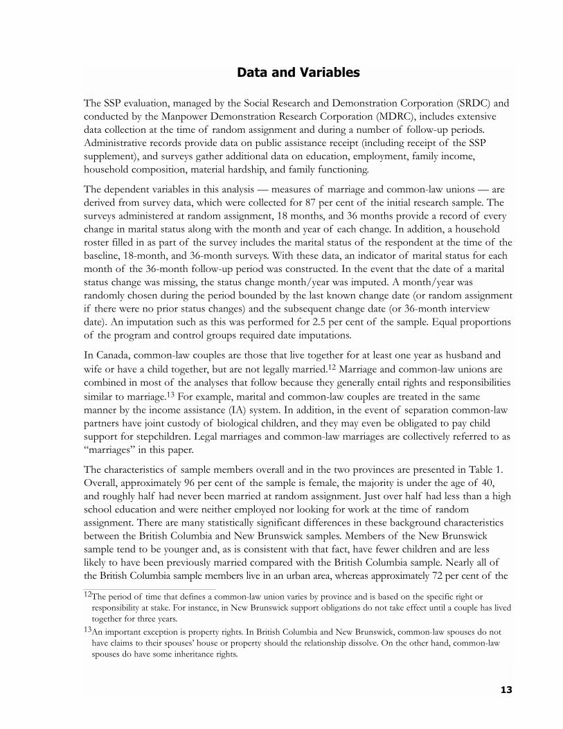
The characteristics of sample members overall and in the two provinces are presented in Table 1.Overall, approximately 96 per cent of the sample is female, the majority is under the age of 40,and roughly half had never been married at random assignment. Just over half had less than a highschool education and were neither employed nor looking for work at the time of randomassignment. There are many statistically significant differences in these background characteristicsbetween the British Columbia and New Brunswick samples. Members of the New Brunswicksample tend to be younger and, as is consistent with that fact, have fewer children and are lesslikely to have been previously married compared with the British Columbia sample. Nearly all ofthe British Columbia sample members live in an urban area, whereas approximately 72 per cent of the12The period of time that defines a common-law union varies by province and is based on the specific right or

responsibility at stake. For instance, in New Brunswick support obligations do not take effect until a couple has livedtogether for three years.

13An important exception is property rights. In British Columbia and New Brunswick, common-law spouses do nothave claims to their spouses� house or property should the relationship dissolve. On the other hand, common-lawspouses do have some inheritance rights.

14

New Brunswick sample lives in an urban area. Sample members in British Columbia are more likely tobe immigrants and are more ethnically diverse compared with sample members in New Brunswick.

Characteristic at Baseline British Columbia New Brunswick Both ProvincesPersonal characteristics (%)

Female 95.6 95.7 95.6Urban residence 92.2 71.8 *** 82.1

Age (%)19-24 18.6 25.8 *** 22.125-29 20.9 20.9 20.930-39 41.6 36.6 *** 39.140-49 16.5 14.3 ** 15.450 or older 2.5 2.5 2.5

Education (%)Less than high school 53.3 53.8 53.6High school, no post-secondary 33.8 36.6 ** 35.2Some post-secondary 12.9 9.5 *** 11.2

Marital status (%)Married or living common-law 1.0 1.1 1.0Never married 43.5 54.1 *** 48.8Divorced, separated, or widowed 54.1 44.1 *** 49.1Expect to be married within 1 year 7.0 6.8 6.9

Children (%)Has 1 child 45.5 53.6 *** 49.5Has 2 children 35.0 33.4 34.2Has 3 or more children 18.2 11.7 *** 15.0Has child less than 6 years old 55.9 52.0 *** 53.9

Work history and labour force statusEver had a paid job (%) 95.3 94.1 ** 94.7Average years worked 8.1 6.6 *** 7.4Labor force status at random assignment (%)

Employed full-time 6.8 6.9 6.8Employed part-time 12.2 13.5 12.9Looking for work, not employed 22.2 22.6 22.4Neither employed nor looking for work 58.8 57.0 57.9

Birthplace and ancestry (%)Not born in Canada 23.4 2.8 *** 13.2Ancestry

Canadian 41.6 59.8 *** 50.6European 61.3 66.6 *** 63.9Asian 8.7 0.3 *** 4.5Latin 3.1 0.4 *** 1.8First Nations 11.5 6.4 *** 9.0Middle Eastern 1.3 0.4 *** 0.9Indian 1.9 0.1 *** 1.0

Language (%)English 95.0 98.8 *** 96.9French 4.7 23.1 *** 13.8Spanish 3.0 0.1 *** 1.4Vietnamese 7.3 0.0 a 2.9Punjabi 0.8 0.0 a 0.4Chinese 1.4 0.0 a 0.7

Sample size 2,503 2,458 4,961

Source: SSP baseline survey.Notes: A two-tailed t-test was applied to differences between the British Columbia and New Brunswick samples. Statistical significance levels are indicated as: ***=1 percent; **=5 percent; *=10 percent. a Statistical tests not performed.

Table 1: Selected Baseline Characteristics of SSP 36-Month Survey Respondents, by Province

15

Appendix B provides evidence on whether random assignment succeeded in generating programand control groups that are similar in their background characteristics. Appendix B compares 36-month survey respondents in the program and control groups on 38 baseline characteristics.At a 10 per cent level of statistical significance, we would expect about 4 of the 38 characteristicsto be significantly different by chance. In British Columbia, 8 of 38 characteristics were significantlydifferent in the program and control groups. In New Brunswick, none of the 38 characteristics wassignificantly different between groups. Because of the British Columbia baseline differencesbetween research groups, in our analysis we test the sensitivity of our results to the inclusion ofcontrol variables that take into account these baseline differences.

17

Empirical Analysis

The goal of the empirical analysis is to estimate the effect of SSP on the propensity to be married.Because these data are generated from an experimental design, any difference in marriage ratesbetween the control group and the program group � the impact � may be attributed to theprogram. Thus, with the experimental design observed and unobserved background characteristicsand changes in the labour markets or other public policies over time should not bias the effect ofthe program on marriage. The marriage decision may be empirically represented as

(3) Mi* = α+βPi+εi

where i is the individuals in the study, P is assignment to the SSP program group (versus actuallytaking up the SSP supplement, which is depicted by S in Equation 2), β1 represents the impact ofSSP on marriage, α is the intercept, and εi is a normally distributed error term.14

The empirical analysis begins with the experimental impacts of SSP on marriage over 36 monthsof follow-up in the full sample, combining British Columbia and New Brunswick. The basicimpact analysis was performed using OLS regression. The empirical results were robust to differentevent-history methodological approaches and logistic regression techniques. The OLS results arepresented for ease of interpretation.15

The SSP evaluation was intentionally structured to test the effects of an identical earningssupplement on the behaviour of single parents in two very different provinces. Because randomassignment for the SSP evaluation occurred within each province, observed and unobservedcharacteristics may vary across the provinces. Prior empirical work finds that unobserved geographicor area effects play some role in estimates of the effects of policies on marital status or fertility(e.g. Moffitt, 1994). In the SSP data, characteristics that can be observed reveal substantialdifferences between the two provinces. As is suggested by Table 1, British Columbia is mostlyurban with a sizeable immigrant population compared with New Brunswick, which is more rural

14The impact of SSP was also estimated in a model that controlled for a number of baseline characteristics as follows:

The independent variables in this equation include a number of baseline or pre-random assignment characteristics.Note that with the experimental design of the study, the estimate of SSP in the unadjusted equation should not beaffected by observed or unobserved characteristics of the program and control groups. Control variables adjust forchance differences in observed background characteristics between the program and control groups. As is discussedlater, inclusion of control variables did not alter the results.

15Event-history methodology is ordinarily preferable to linear regression when the dependent variable is an event andsome of the observations have not experienced the event at the time of observation or have left the sample (i.e.some events are right censored). Event-history models are able to incorporate the time that observations were at riskbefore being censored, or before experiencing the event, when estimating coefficients (Allison, 1995). In this analysis,the OLS estimates are comparable to the event-history results because almost all of the censored cases were at riskfor approximately 36 months; therefore, censoring is not informative. The Kaplan-Meier, Cox, and logistic regressionresults are available from the authors upon request.

∑=

+++=K

kiikii XPM

2

1* εββα

and has few immigrants. With these contextual differences in mind, the estimating equation wouldideally be expanded as follows:

(4) Mis* = α+βPi+γs+εis

where i represents individuals in the study, s represents provinces in the study, and γs is a province-fixed effect intended to capture unmeasured social, cultural, and other factors that vary acrossprovinces.16 Because only two provinces were included in the SSP evaluation, we separatelyestimate the effect of SSP for each province:

(5) Mis* = αs+βsPis+εis

where s = NB for a separate equation with the New Brunswick sample and s = BC for a separateequation with the British Columbia sample. Noting Equation 5 in the context of Equation 4 isuseful in highlighting that differences in the effect of SSP may be accounted for by unobservedsocial, cultural, and other factors that vary by province.

The experimental design of the data also allows us to address adequately the endogenousrelationship of labour supply to marriage decisions (see Eissa & Hoynes, 1999, for a treatment ofthese endogeneity issues with non-experimental data). One direct way to examine theseendogeneity issues is to compare the impacts of SSP on marriage with the impacts of SSP onemployment and/or income. The indirect way to examine these endogeneity issues is to use theexperiment, whether or not a sample member is in the program group, as an instrument to predictthe effects of employment and earnings on marriage in a two-stage instrumental variables model.In this paper, the endogeneity of employment and income are examined primarily throughexperimental techniques by comparing the impacts of SSP on employment and income withimpacts on marriage.

18

16Note that unobserved individual differences within a province should not bias the results since random assignmenttook place within each province.

Empirical Results

SSP�s effect on marriage

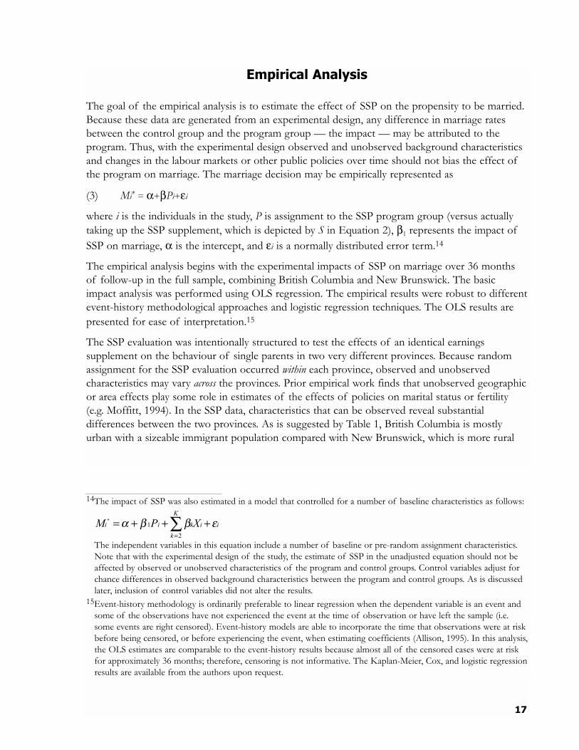
As has been explained, it is uncertain whether to expect SSP to have a positive, negative, or neutraleffect on marriage. Therefore, the first hypothesis tested in this section is simply did SSP have animpact on marriage? Second, because SSP was implemented in two diverse locales, this section alsoexamines whether or not SSP�s effect on marriage varied by province. Table 2a shows theexperimental difference in the incidence of marriage over 36 months of follow-up, the averagenumber of months married, and the percentage married or common-law in the last month offollow-up. Figures 4 through 7 display the pattern of impacts on marriage by month.

When the two provinces are combined, SSP did not have an effect on marriage at any point over36 months. Figure 4 shows that similar percentages of program and control group members weremarried in each of 36 months of follow-up. Table 2a further shows that SSP had no impact onmarriage within the follow-up period, the number of months married, or being married orcommon-law in the last month of the 36-month follow-up.

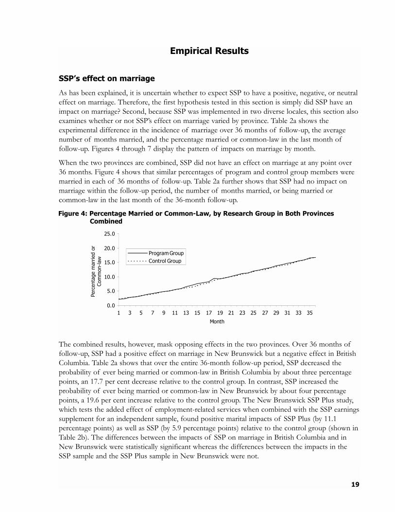
The combined results, however, mask opposing effects in the two provinces. Over 36 months offollow-up, SSP had a positive effect on marriage in New Brunswick but a negative effect in BritishColumbia. Table 2a shows that over the entire 36-month follow-up period, SSP decreased theprobability of ever being married or common-law in British Columbia by about three percentagepoints, an 17.7 per cent decrease relative to the control group. In contrast, SSP increased theprobability of ever being married or common-law in New Brunswick by about four percentagepoints, a 19.6 per cent increase relative to the control group. The New Brunswick SSP Plus study,which tests the added effect of employment-related services when combined with the SSP earningssupplement for an independent sample, found positive marital impacts of SSP Plus (by 11.1percentage points) as well as SSP (by 5.9 percentage points) relative to the control group (shown inTable 2b). The differences between the impacts of SSP on marriage in British Columbia and inNew Brunswick were statistically significant whereas the differences between the impacts in theSSP sample and the SSP Plus sample in New Brunswick were not.

19

0.0

5.0

10.0

15.0

20.0

25.0

1 3 5 7 9 11 13 15 17 19 21 23 25 27 29 31 33 35

Month


Figure 4: Percentage Married or Common-Law, by Research Group in Both Provinces Combined

Perc

enta

ge m

arrie

d or

Com

mon

-law

Are the impacts on marriage in British Columbia and New Brunswick robust? Robustnesswas tested in several ways: by looking at trends in impacts over time, by using alternative statisticalprocedures to estimate impacts on marriage, by including control variables in estimating equations,and by examining impact results for a number of subgroups. These robustness checks revealed thatthe findings in general are robust, though the degree of robustness differs slightly for eachprovince. Across these robustness checks, the positive marriage effect in New Brunswick holds upand, in many cases, achieves high levels of statistical significance (i.e. p-values of at least 0.0001).Though the negative marriage effect in British Columbia also holds up, it does not achieve thesame high levels of statistical significance as in New Brunswick. For this reason and because, aswill be discussed, the pathways by which SSP affected marriage are more tentative in BritishColumbia, we place slightly more confidence in the positive findings on marriage in NewBrunswick than we do on the negative findings on marriage in British Columbia.

20

Program Control Difference StandardOutcome Group Group (Impact) Error ChangeBoth provincesEver married or common-law, month 1-36 (%) 19.5 19.2 0.3 (1.1) 1.5%Number of months married or common-law, month 1-36 3.3 3.3 0.0 (0.2) 1.3%Married or common-law at 36-month interview (%) 17.4 17.3 0.1 (1.1) 0.7%

Married at 36-month interview 8.8 9.5 -0.6 (0.8) -6.8%Common-law at 36-month interview 8.6 7.8 0.8 (0.8) 10.0%

Sample size (4,961) 2,503 2,458

British ColumbiaEver married or common-law, month 1-36 (%) 14.6 17.7 -3.1 ** (1.5) -17.8%Number of months married or common-law, month 1-36 2.3 3.0 -0.7 ** (0.3) -22.4%Married or common-law at 36-month interview (%) 13.5 15.5 -2.0 (1.4) -12.7%

Married at 36-month interview 7.7 9.7 -2.0 * (1.1) -20.1%Common-law at 36-month interview 5.8 5.8 0.0 (0.9) -0.3%

Sample size (2,537) 1,296 1,241

New BrunswickEver married or common-law, month 1-36 (%) 24.8 20.7 4.1 ** (1.7) 19.6%Number of months married or common-law, month 1-36 4.4 3.5 0.8 ** (0.4) 23.5%Married or common-law at 36-month interview (%) 21.6 19.1 2.5 (1.6) 13.0%

Married at 36-month interview 10.0 9.3 0.7 (1.2) 8.0%Common law at 36-month interview 11.6 9.9 1.7 (1.3) 17.6%

Sample size (2,424) 1,207 1,217

Source: Calculations from SSP surveys.Notes: A two-tailed t-test was applied to differences between the outcomes for the program and control groups. Statistical significance levels are indicated as: * = 10 percent; ** = 5 percent; *** = 1 percent.

Table 2a: SSP Impacts on Marriage and Common-Law Unions Over Three Years of Follow-Up

21

Difference: Difference: Difference:SSP Plus SSP vs. SSP Plus

SSP Plus SSP Control vs. Control Standard Control Standard vs. SSP Standard Outcome Group Group Group (Impact) Error (Impact) Error (Impact) ErrorNew BrunswickEver married or common law month 1-36 (%) 28.5 23.3 17.4 11.1 *** (3.6) 5.9 * (3.6) 5.1 (3.6)Number of months married or common law month 1-36 4.8 3.4 3.5 1.4 * (0.8) 0.0 (0.8) 1.0 (0.8)( ) ( )Sample size (820) 274 270 276


Table 2b: SSP Plus Impacts on Marriage and Common-Law Unions Over Three Years of Follow-Up

The negative effect in British Columbia and the positive effect in New Brunswick were consistentover time. Figure 5 shows that in British Columbia SSP had a consistently negative effect onmarriage in each month over 36 months of follow-up. The negative program/control differencewas statistically significant in every month but one starting in month nine. Figure 6 shows that inNew Brunswick SSP increased marriage in every month of follow-up. The positive impact onmarriage in New Brunswick was significant in months 11 through 35.17 In addition, SSP�s effects inNew Brunswick are confirmed with an independent sample, the SSP Plus sample, that experiencedan intervention similar to that in the main SSP experiment and that has similar characteristics toNew Brunswick sample members in the main SSP experiment. Compared with the control group,the SSP Plus experiment produced effects on employment and income (not shown) and onmarriage (Figure 7) that were similar to effects produced in the main SSP experiment in NewBrunswick.

22

0.0

5.0

10.0

15.0

20.0

25.0

1 3 5 7 9 11 13 15 17 19 21 23 25 27 29 31 33 35

Month


17Between months 35 and 36, the New Brunswick impact decreased only slightly, from 3.1 to 2.6 percentage points,but the month 36 impact was no longer statistically significant at the 10 per cent level.

0.0

5.0

10.0

15.0

20.0

25.0

1 3 5 7 9 11 13 15 17 19 21 23 25 27 29 31 33 35

Month


Figure 5: Percentage Married or Common-Law, by Research Group in British Columbia

Figure 6: Percentage Married or Common-Law, by Research Group in New Brunswick

Perc

enta

ge m

arrie

d or

Com

mon

-law

Perc

enta

ge m

arrie

d or

Com

mon

-law

The positive and negative effects of SSP in each province are robust to different statisticalmethods. When Wilcoxon and log-rank tests were applied to the Kaplan-Meier survival curves forthe program and control groups within each province, the negative difference between the survivalcurves of the program and control groups in British Columbia and the positive difference in NewBrunswick was statistically significant. The marital impact results by province and subgroup werereproduced using Cox proportional hazards models. The risk ratios from these modelscorresponded closely to the OLS regression results. The Cox risk ratios mirrored the percentagechange, the impact divided by the control group mean, from OLS. The significance levels from theCox models were similar to the significance levels from the OLS models. In addition, logisticregression yielded results consistent with the OLS estimates.

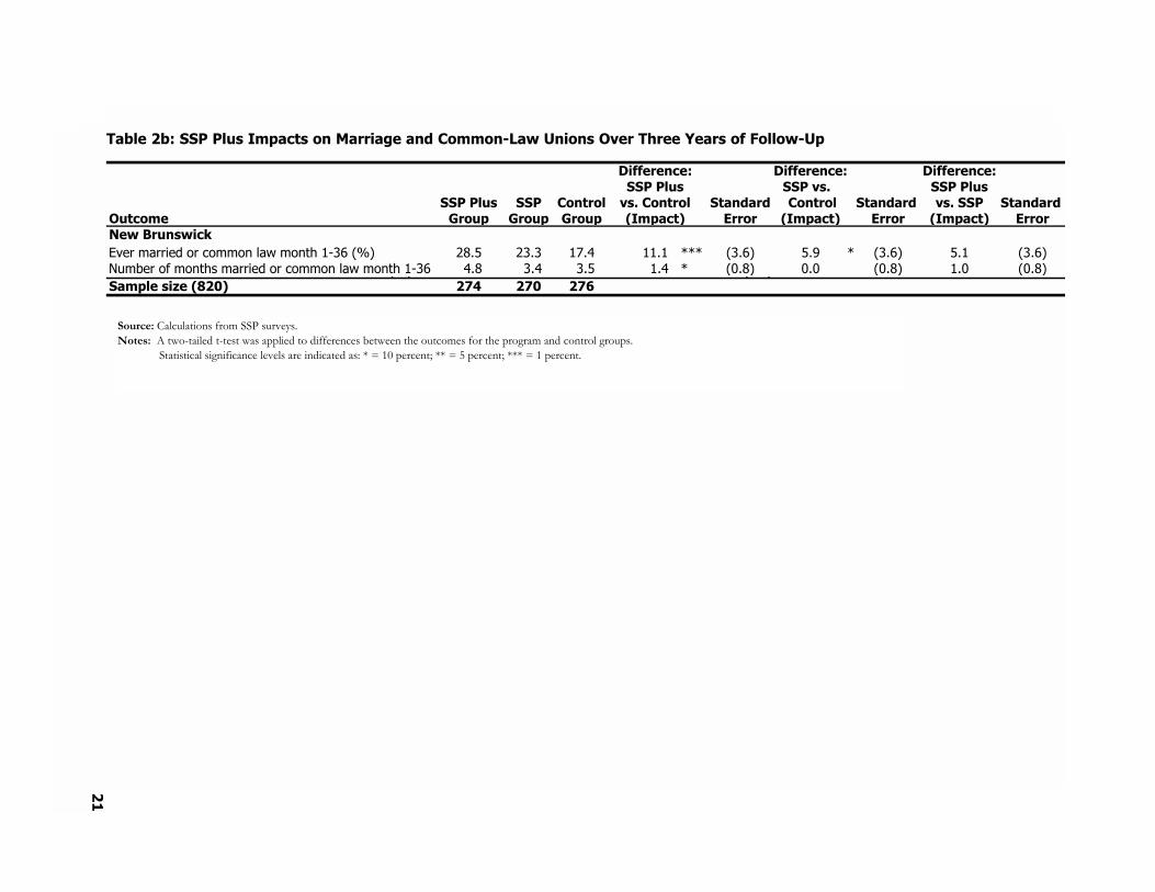
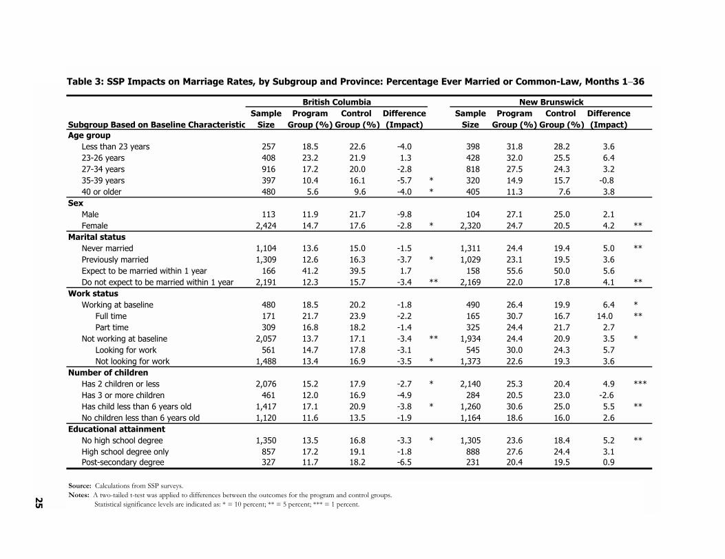
The robustness of the results is further suggested by the fact that the direction of the NewBrunswick and British Columbia impacts is uniform across different subgroups of the sample.Table 3 presents results for subgroups defined by baseline characteristics such as age, gender,number of children, educational attainment, and employment and marital status at baseline withineach province. SSP�s effect on marriage for British Columbia was negative for almost everysubgroup.18 The effect on marriage in New Brunswick was positive for all but one subgroup.

When control variables were included to adjust for differences in background characteristicsbetween the research groups, the New Brunswick estimates were unaffected but the BritishColumbia results were slightly attenuated. Random assignment ensures that the program andcontrol groups are similar in their background characteristics. However, Appendix B reveals a fewdifferences between the background characteristics of program and control group members,especially in British Columbia, either due to chance or to differential patterns of surveynonresponse in the two research groups. When we control for the standard set of covariates used

23

18The large significant negative impact on marriage for males in British Columbia is striking. Because the sample ofmales is small, however, excluding males from the total sample does not affect the general impact findings (notshown).

0

5

10

15

20

25

30

1 3 5 7 9 11 13 15 17 19 21 23 25 27 29 31 33 35

Month

SSP Plus GroupRegular SSP GroupControl Group

Figure 7: Percentage Married or Common-Law, by Research Group in New BrunswickSSP Plus Study

Perc

enta

ge m

arrie

d or

Com

mon

-law

in SSP�s economic analyses, the New Brunswick results remain the same as the unadjustedestimates.19 In British Columbia, the impact on ever being married and months of marriage overthe entire 36-month follow-up period are similarly unaffected when these control variables areincluded. However, the impacts of SSP on marriage in each individual month of follow-up inBritish Columbia become weaker and less significant when these control variables are added. Tofurther test the sensitivity of the British Columbia results, we estimated a regression with adifferent set of covariates chosen because they are theoretically related to marriage.20 Using thissecond set of control variables, the British Columbia results are similar to the unadjusted results.21

On the basis of this and other pieces of evidence, we conclude that the results in each provinceare robust, but the positive New Brunswick results are slightly stronger than the negative BritishColumbia results.

Mechanisms by which SSP affected marriage

The subgroup results in Table 3 allow us to somewhat untangle which theoretical effects seem topredominate in each province. The decrease in marriage in British Columbia may have beenassociated with an independence effect (increased income allowing women to postpone or forgomarriage), time constraints on dating imposed by full-time work, or increased stress caused by thedemands of full-time work combined with parenting. If the negative effect of SSP on marriage isassociated with the increased time constraints and stress from work, then we would expect a largernegative effect on marriage for the subgroup not working at baseline compared with the subgroupthat was employed at baseline. On the other hand, if the negative effect on marriage is driven byan independence effect caused by increased income, then the negative impact on marriage wouldalso appear for those employed full time at baseline.

For those employed at baseline in British Columbia, when part-time and full-time employments aretaken together, SSP�s effects on marriage are neutral, providing some evidence against theindependence hypothesis. However, for those employed full time at baseline, for whom the timedemands and stress of work were unlikely to increase as a result of SSP, there is a negative effectof SSP of a similar magnitude as for those not working at baseline. On the basis of this evidence,none of the theoretical effects can be ruled out.

The increase in marriage in New Brunswick may have been associated with exposure to socialnetworks, increased self-esteem through work, the increased income provided by SSP, or the removalof the income assistance marriage disincentive. Table 3 shows that the largest positive impact onmarriage, 14 percentage points, corresponds to recipients who were employed full time at baseline.Because this group was already immersed in the labour force at baseline and is most likely to benefitfrom the income windfall of SSP, the large impact for this group supports the hypothesis thatincome drove increases in marriage as opposed to exposure to new social networks or increased self-esteem from work.

24

19The standard set of covariates used in SSP�s economic analyses includes the following variables: random assignmentcohort, age of youngest child, marital status at baseline, educational attainment, can borrow money from family orfriends, has had the blues, has physical problem, has emotional problem, age, prior welfare receipt, and prior earnings.

20This set of covariates included those in the standard economic models plus urban residence, total number ofchildren, working at baseline, speaks French, expects to be married within one year, and ancestry.

21Regression-adjusted impact estimates are available from the authors upon request.

British Columbia New BrunswickSample Program Control Difference Sample Program Control Difference

Subgroup Based on Baseline Characteristic Size Group (%) Group (%) (Impact) Size Group (%) Group (%) (Impact)Age group

Less than 23 years 257 18.5 22.6 -4.0 398 31.8 28.2 3.623-26 years 408 23.2 21.9 1.3 428 32.0 25.5 6.427-34 years 916 17.2 20.0 -2.8 818 27.5 24.3 3.235-39 years 397 10.4 16.1 -5.7 * 320 14.9 15.7 -0.840 or older 480 5.6 9.6 -4.0 * 405 11.3 7.6 3.8

SexMale 113 11.9 21.7 -9.8 104 27.1 25.0 2.1Female 2,424 14.7 17.6 -2.8 * 2,320 24.7 20.5 4.2 **

Marital statusNever married 1,104 13.6 15.0 -1.5 1,311 24.4 19.4 5.0 **Previously married 1,309 12.6 16.3 -3.7 * 1,029 23.1 19.5 3.6Expect to be married within 1 year 166 41.2 39.5 1.7 158 55.6 50.0 5.6Do not expect to be married within 1 year 2,191 12.3 15.7 -3.4 ** 2,169 22.0 17.8 4.1 **

Work statusWorking at baseline 480 18.5 20.2 -1.8 490 26.4 19.9 6.4 *

Full time 171 21.7 23.9 -2.2 165 30.7 16.7 14.0 **Part time 309 16.8 18.2 -1.4 325 24.4 21.7 2.7

Not working at baseline 2,057 13.7 17.1 -3.4 ** 1,934 24.4 20.9 3.5 *Looking for work 561 14.7 17.8 -3.1 545 30.0 24.3 5.7Not looking for work 1,488 13.4 16.9 -3.5 * 1,373 22.6 19.3 3.6

Number of childrenHas 2 children or less 2,076 15.2 17.9 -2.7 * 2,140 25.3 20.4 4.9 ***Has 3 or more children 461 12.0 16.9 -4.9 284 20.5 23.0 -2.6Has child less than 6 years old 1,417 17.1 20.9 -3.8 * 1,260 30.6 25.0 5.5 **No children less than 6 years old 1,120 11.6 13.5 -1.9 1,164 18.6 16.0 2.6

Educational attainmentNo high school degree 1,350 13.5 16.8 -3.3 * 1,305 23.6 18.4 5.2 **High school degree only 857 17.2 19.1 -1.8 888 27.6 24.4 3.1Post-secondary degree 327 11.7 18.2 -6.5 231 20.4 19.5 0.9


Table 3: SSP Impacts on Marriage Rates, by Subgroup and Province: Percentage Ever Married or Common-Law, Months 1−36

25

26

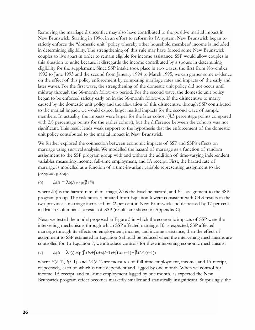
Removing the marriage disincentive may also have contributed to the positive marital impact inNew Brunswick. Starting in 1996, in an effort to reform its IA system, New Brunswick began tostrictly enforce the �domestic unit� policy whereby other household members� income is includedin determining eligibility. The strengthening of this rule may have forced some New Brunswickcouples to live apart in order to remain eligible for income assistance. SSP would allow couples inthis situation to unite because it disregards the income contributed by a spouse in determiningeligibility for the supplement. Since SSP intake took place in two waves, the first from November1992 to June 1993 and the second from January 1994 to March 1995, we can garner some evidenceon the effect of this policy enforcement by comparing marriage rates and impacts of the early andlater waves. For the first wave, the strengthening of the domestic unit policy did not occur untilmidway through the 36-month follow-up period. For the second wave, the domestic unit policybegan to be enforced strictly early on in the 36-month follow-up. If the disincentive to marrycaused by the domestic unit policy and the alleviation of this disincentive through SSP contributedto the marital impact, we would expect larger marital impacts for the second wave of samplemembers. In actuality, the impacts were larger for the later cohort (4.3 percentage points comparedwith 2.8 percentage points for the earlier cohort), but the difference between the cohorts was notsignificant. This result lends weak support to the hypothesis that the enforcement of the domesticunit policy contributed to the marital impact in New Brunswick.

We further explored the connection between economic impacts of SSP and SSP�s effects onmarriage using survival analysis. We modelled the hazard of marriage as a function of randomassignment to the SSP program group with and without the addition of time-varying independentvariables measuring income, full-time employment, and IA receipt. First, the hazard rate ofmarriage is modelled as a function of a time-invariant variable representing assignment to theprogram group:

(6) hi(t) = λ0(t) exp(β1Pi)

where h(t) is the hazard rate of marriage, λ0 is the baseline hazard, and P is assignment to the SSPprogram group. The risk ratios estimated from Equation 6 were consistent with OLS results in thetwo provinces; marriage increased by 22 per cent in New Brunswick and decreased by 17 per centin British Columbia as a result of SSP (results are shown in Appendix C).

Next, we tested the model proposed in Figure 3 in which the economic impacts of SSP were theintervening mechanisms through which SSP affected marriage. If, as expected, SSP affectedmarriage through its effects on employment, income, and income assistance, then the effect ofassignment to SSP estimated in Equation 6 should be reduced when the intervening mechanisms arecontrolled for. In Equation 7, we introduce controls for these intervening economic mechanisms:

(7) hi(t) = λ0(t)exp(β1Pi+β2Ei(t−1)+β3Ii(t−1)+β4IAi(t−1))

where E(t−1), I(t−1), and IA(t−1) are measures of full-time employment, income, and IA receipt,respectively, each of which is time dependent and lagged by one month. When we control forincome, IA receipt, and full-time employment lagged by one month, as expected the NewBrunswick program effect becomes markedly smaller and statistically insignificant. Surprisingly, the

27

opposite is true for the British Columbia sample. Here, when we control for income, employment,and IA receipt, the negative program effect becomes larger and more statistically significant. Theseresults find support for the expected relation between SSP�s economic and marital impacts in NewBrunswick. In British Columbia the mechanism by which SSP affected marriage is less clear.22

Why did SSP�s effect on marriage differ by province?

The effects of income and employment did not vary by province.23 As shown in theconceptual model above, one way that SSP was predicted to affect marriage is through its effectson income and employment. Can differences in SSP�s impacts on income and employment byprovince help to explain its different effects on marriage? Tables 4 and 5 provide evidence to testhow SSP may have affected marriage by presenting impacts on average monthly full-timeemployment and on income (from SSP, welfare benefits, and earnings) by subgroup. The first thingto note is that the SSP program increased income and full-time employment for nearly everysubgroup in both provinces. The second noteworthy observation is that there is not a simplerelation between impacts on income and full-time employment and impacts on marriage; largerimpacts on income and full-time employment were not consistently associated with larger orsmaller impacts on marriage.24 However, a general trend emerges in each province. In BritishColumbia SSP increased income and full-time employment and decreased marriage in nearly everysubgroup. In New Brunswick SSP also increased income and full-time employment, but increasedmarriage in nearly every subgroup.

The characteristics of the sample did not vary by province. Could the differences in samplecharacteristics between the two provinces shown in Table 1 help to explain differences in impactson marriage? Table 1 showed that the British Columbia and New Brunswick sample members weresignificantly different in many of their background characteristics. Therefore, one possibleexplanation for the difference in the SSP program impact on marriage is that sample characteristicsassociated with positive impacts were more common in New Brunswick while characteristicsassociated with negative impacts were more common in British Columbia. For example, if SSP hada positive effect on marriage for all young sample members then, because the New Brunswicksample was younger than the British Columbia sample, the New Brunswick sample would exhibitmore of this positive marital impact.

22Note that because SSP is a voluntary program it is expected that the effects of SSP on full-time employment,income, and IA receipt occur primarily for those welfare recipients who take up the supplement offer. A simplecomparison of marriage rates between SSP �takers� with members of the control group does not preserve theexperimental design of the experiment. Other non-experimental techniques may be utilized to examine the relationbetween �take-up� of the SSP supplement and marriage. This kind of analysis is beyond the scope of the currentpaper.

23SSP had no significant impact on fertility for the full sample or separately for each province.24In fact, very preliminary non-experimental estimates from instrumental variables analysis find that overall, for the

combined SSP and SSP Plus sample, income has a negative effect on marriage and employment has a positive effecton marriage. This analysis used an indicator for being in the SSP experimental group, an indicator for being in theSSP Plus experimental group, and the interaction of being in the SSP group and in New Brunswick as instrumentsto predict employment and income. The predicted effects of income and employment were then used as covariatesin an equation with marriage as the dependent variable (with the appropriate standard error adjustments).

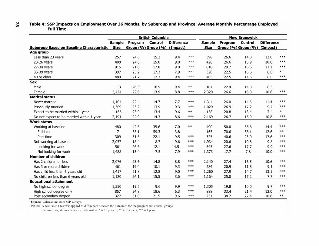
28


Subgroup Based on Baseline Characteristic Size Group (%) Group (%) (Impact) Size Group (%) Group (%) (Impact)Age group

Less than 23 years 257 24.6 15.2 9.4 *** 398 26.6 14.0 12.6 ***23-26 years 408 24.0 15.0 9.0 *** 428 26.6 15.9 10.8 ***27-34 years 916 21.8 12.8 9.0 *** 818 29.7 16.6 13.1 ***35-39 years 397 25.2 17.3 7.9 ** 320 22.5 16.6 6.0 *40 or older 480 21.7 12.3 9.4 *** 405 22.5 14.6 8.0 ***

SexMale 113 26.3 16.9 9.4 ** 104 22.4 14.0 8.5Female 2,424 22.6 13.9 8.8 *** 2,320 26.6 16.0 10.6 ***

Marital statusNever married 1,104 22.4 14.7 7.7 *** 1,311 26.0 14.6 11.4 ***Previously married 1,309 23.2 13.9 9.3 *** 1,029 26.9 17.2 9.7 ***Expect to be married within 1 year 166 23.0 13.4 9.6 ** 158 20.8 13.4 7.4 *Do not expect to be married within 1 year 2,191 22.9 14.3 8.6 *** 2,169 26.7 15.9 10.8 ***

Work statusWorking at baseline 480 42.6 35.6 7.0 ** 490 50.0 35.6 14.4 ***

Full time 171 63.1 59.3 3.8 165 70.6 58.1 12.6 **Part time 309 31.6 22.1 9.5 *** 325 40.6 23.0 17.6 ***

Not working at baseline 2,057 18.4 8.7 9.6 *** 1,934 20.6 10.8 9.8 ***Looking for work 561 26.6 12.1 14.5 *** 545 27.6 17.7 9.9 ***Not looking for work 1,488 15.4 7.5 7.9 *** 1,373 17.7 7.8 10.0 ***

Number of childrenHas 2 children or less 2,076 23.6 14.8 8.8 *** 2,140 27.4 16.5 10.6 ***Has 3 or more children 461 19.4 10.1 9.3 *** 284 20.9 11.8 9.1 ***Has child less than 6 years old 1,417 21.8 12.8 9.0 *** 1,260 27.9 14.7 13.1 ***No children less than 6 years old 1,120 24.1 15.5 8.6 *** 1,164 25.0 17.2 7.7 ***

Educational attainmentNo high school degree 1,350 19.5 9.6 9.9 *** 1,305 19.8 10.0 9.7 ***High school degree only 857 24.8 18.6 6.3 *** 888 33.4 21.4 12.0 ***Post-secondary degree 327 31.0 21.5 9.6 *** 231 38.2 27.4 10.8 **


Table 4: SSP Impacts on Employment Over 36 Months, by Subgroup and Province: Average Monthly Percentage Employed Full Time

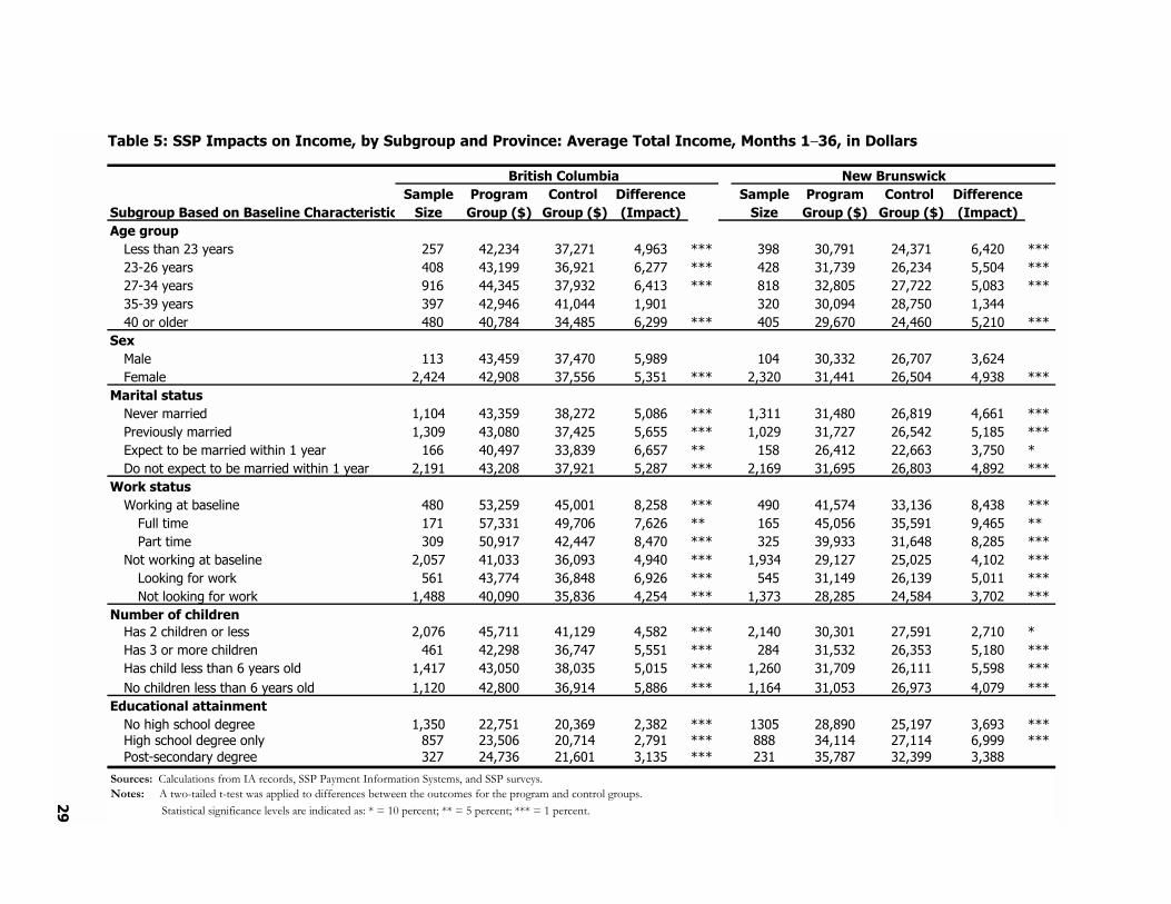
29


Subgroup Based on Baseline Characteristic Size Group ($) Group ($) (Impact) Size Group ($) Group ($) (Impact)Age group

Less than 23 years 257 42,234 37,271 4,963 *** 398 30,791 24,371 6,420 ***23-26 years 408 43,199 36,921 6,277 *** 428 31,739 26,234 5,504 ***27-34 years 916 44,345 37,932 6,413 *** 818 32,805 27,722 5,083 ***35-39 years 397 42,946 41,044 1,901 320 30,094 28,750 1,34440 or older 480 40,784 34,485 6,299 *** 405 29,670 24,460 5,210 ***

SexMale 113 43,459 37,470 5,989 104 30,332 26,707 3,624Female 2,424 42,908 37,556 5,351 *** 2,320 31,441 26,504 4,938 ***

Marital statusNever married 1,104 43,359 38,272 5,086 *** 1,311 31,480 26,819 4,661 ***Previously married 1,309 43,080 37,425 5,655 *** 1,029 31,727 26,542 5,185 ***Expect to be married within 1 year 166 40,497 33,839 6,657 ** 158 26,412 22,663 3,750 *Do not expect to be married within 1 year 2,191 43,208 37,921 5,287 *** 2,169 31,695 26,803 4,892 ***

Work statusWorking at baseline 480 53,259 45,001 8,258 *** 490 41,574 33,136 8,438 ***

Full time 171 57,331 49,706 7,626 ** 165 45,056 35,591 9,465 **Part time 309 50,917 42,447 8,470 *** 325 39,933 31,648 8,285 ***

Not working at baseline 2,057 41,033 36,093 4,940 *** 1,934 29,127 25,025 4,102 ***Looking for work 561 43,774 36,848 6,926 *** 545 31,149 26,139 5,011 ***Not looking for work 1,488 40,090 35,836 4,254 *** 1,373 28,285 24,584 3,702 ***

Number of childrenHas 2 children or less 2,076 45,711 41,129 4,582 *** 2,140 30,301 27,591 2,710 *Has 3 or more children 461 42,298 36,747 5,551 *** 284 31,532 26,353 5,180 ***Has child less than 6 years old 1,417 43,050 38,035 5,015 *** 1,260 31,709 26,111 5,598 ***No children less than 6 years old 1,120 42,800 36,914 5,886 *** 1,164 31,053 26,973 4,079 ***

Educational attainmentNo high school degree 1,350 22,751 20,369 2,382 *** 1305 28,890 25,197 3,693 ***High school degree only 857 23,506 20,714 2,791 *** 888 34,114 27,114 6,999 ***Post-secondary degree 327 24,736 21,601 3,135 *** 231 35,787 32,399 3,388

Sources: Calculations from IA records, SSP Payment Information Systems, and SSP surveys.Notes: A two-tailed t-test was applied to differences between the outcomes for the program and control groups. Statistical significance levels are indicated as: * = 10 percent; ** = 5 percent; *** = 1 percent.

Table 5: SSP Impacts on Income, by Subgroup and Province: Average Total Income, Months 1−36, in Dollars

The evidence suggests that sample characteristics do not help to explain the differences in maritalimpacts between the two provinces. First, the subgroup results in Table 3 show that impacts onmarriage are negative for almost every subgroup in British Columbia and positive for almost everysubgroup in New Brunswick. Estimates of conditional impacts provide further evidence againstthe hypothesis that sample characteristics explain the opposite marital impacts in the two provinces.The conditional impact estimates allow the program effect on marriage to vary by province and bya number of background characteristics. After taking into account the variation in program impactsassociated with baseline characteristics, program effects in the two provinces remain significantlydifferent. Conditional impact estimates were derived from the following equation:

K M

(8) Mi* = α+β1Pi+β2Ni+β3NiPi+ΣβkXi+ΣβmXiPi+εi

k=4 m=K

where M is ever married during the 36 month follow-up period, P represents assignment to theSSP program group, N indicates being in the New Brunswick sample, NP is the NewBrunswick/SSP program group interaction term, X is a vector of individual characteristics, and XPis a vector of individual characteristics interacted with SSP program group membership.

The vector of covariates (X) includes all of the baseline characteristics presented in Table 1. Thevariable of interest in this equation is the New Brunswick/program group interaction term (NP).The coefficient on this variable (β3) indicates the net difference in the marital impacts in NewBrunswick versus British Columbia after accounting for the variation in program impactsassociated with baseline characteristics. The coefficient on the New Brunswick/program groupinteraction term was 0.081, indicating that the net difference between the New Brunswick andBritish Columbia program impacts on marriage was 8.1 percentage points. This difference issignificant at the one per cent level. This evidence suggests that observed baseline differencesbetween the New Brunswick and British Columbia samples do not account for differences in NewBrunswick and British Columbia program impacts on marital status.

Marriage markets may vary by province. Differences in the supply of and quality of eligiblespouses in a given geographic area, the �marriage market,� may explain the differences in impactsbetween the provinces. Table 6 presents some characteristics of the provinces that proxy themarriage market. The ratio of unmarried men to women in each province gives a sense of thenumber of potential spouses. As is shown in Table 6, this ratio is similar in New Brunswick andBritish Columbia. Prior research has suggested that the employment status of potential malespouses is also important (Wilson & Neckerman, 1987). The unemployment rate for men in NewBrunswick (16.7 per cent) was considerably higher than for men in British Columbia (9.8 per cent).On the basis of this difference, we would expect higher marriage rates in British Columbiacompared with New Brunswick. However, marriage rates are actually higher in New Brunswickthan in British Columbia in both the program and control group. The proxies for marriage marketcharacteristics � sex ratios and male unemployment rates � do not help to explain the differencesin marriage impacts in the two provinces.

30

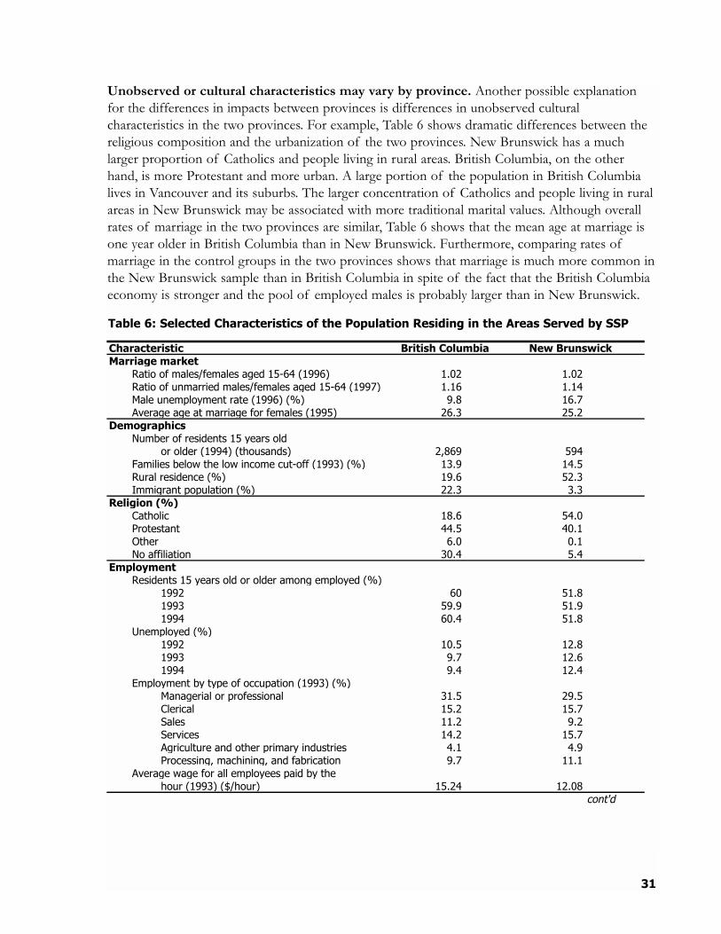
31

Unobserved or cultural characteristics may vary by province. Another possible explanationfor the differences in impacts between provinces is differences in unobserved culturalcharacteristics in the two provinces. For example, Table 6 shows dramatic differences between thereligious composition and the urbanization of the two provinces. New Brunswick has a muchlarger proportion of Catholics and people living in rural areas. British Columbia, on the otherhand, is more Protestant and more urban. A large portion of the population in British Columbialives in Vancouver and its suburbs. The larger concentration of Catholics and people living in ruralareas in New Brunswick may be associated with more traditional marital values. Although overallrates of marriage in the two provinces are similar, Table 6 shows that the mean age at marriage isone year older in British Columbia than in New Brunswick. Furthermore, comparing rates ofmarriage in the control groups in the two provinces shows that marriage is much more common inthe New Brunswick sample than in British Columbia in spite of the fact that the British Columbiaeconomy is stronger and the pool of employed males is probably larger than in New Brunswick.

Characteristic British Columbia New BrunswickMarriage market

Ratio of males/females aged 15-64 (1996) 1.02 1.02Ratio of unmarried males/females aged 15-64 (1997) 1.16 1.14Male unemployment rate (1996) (%) 9.8 16.7Average age at marriage for females (1995) 26.3 25.2

DemographicsNumber of residents 15 years old

or older (1994) (thousands) 2,869 594Families below the low income cut-off (1993) (%) 13.9 14.5Rural residence (%) 19.6 52.3Immigrant population (%) 22.3 3.3

Religion (%)Catholic 18.6 54.0Protestant 44.5 40.1Other 6.0 0.1No affiliation 30.4 5.4

EmploymentResidents 15 years old or older among employed (%)

1992 60 51.81993 59.9 51.91994 60.4 51.8

Unemployed (%)1992 10.5 12.81993 9.7 12.61994 9.4 12.4

Employment by type of occupation (1993) (%)Managerial or professional 31.5 29.5Clerical 15.2 15.7Sales 11.2 9.2Services 14.2 15.7Agriculture and other primary industries 4.1 4.9Processing, machining, and fabrication 9.7 11.1

Average wage for all employees paid by thehour (1993) ($/hour) 15.24 12.08

cont'd

Table 6: Selected Characteristics of the Population Residing in the Areas Served by SSP

32

Focus group transcripts provide further support for the role of unobserved cultural differencesbetween the provinces in explaining the pattern of marital impacts. While many focus groupparticipants in general discussed a desire to get married, only focus group participants in BritishColumbia placed a higher premium on being financially independent, at least in the short term andparticularly from abusive relationships.

Table 6: Selected Characteristics of the Population Residing in the Areas Served by SSP(cont�d)

Characteristic British Columbia New BrunswickWelfare

IA cases (1993) 193,825 42,123Percentage of IA cases that are

single-parent families (1993) 24.8 30.8Basic monthly IA grant to single parent

with 2children (1995) ($) 1,152 747SSP earnings supplement program

SSP income: Monthly earnings and SSP supplementassuming minimum wage and 30 hours/week ($) 1,932 1,575

Ratio of SSP income to basic monthly IA grantto single mother and 2 children 1.8 2.2

Sources: Statistics Canada, Mijanovich & Long (1995), Card & Robins (1996).

33

Discussion and Conclusion

Past research has shown that changes in welfare policies can affect family formation. However, themagnitude and direction of these effects are uncertain, partly because of methodological weaknessesin prior studies, but also because the sets of policies and the contexts they have operated in havebeen diverse. SSP provides a unique opportunity to study the effect on marriage of a simple andeasily replicated earnings supplement program tested in two geographically diverse regions. Thepotential ease of replication of the SSP program design and the availability of experimental resultsin two different provinces represent advantages over prior research in this area.

The set of theoretical positive and negative effects outlined in this paper suggests that it is notclear whether to expect the net effect of the SSP program on marriage to be positive or negative.By removing the marriage disincentive, SSP may increase marriage. However, increasedemployment and increased income due to SSP may affect the propensity to marry either positivelyor negatively.

Our empirical findings show that although on average SSP had no effect on marriage, it had aconsistent effect on marriage over 36 months of follow-up and across subgroups by province:consistently positive in New Brunswick and consistently negative in British Columbia. Findings inthe two provinces are generally robust, although findings in New Brunswick are more robust thanfindings in British Columbia. In New Brunswick, the positive effect is a likely outcome of theincreased income from SSP. There is evidence against the competing hypothesis that marriageincreased by virtue of increased exposure to social networks or self-esteem through working. InBritish Columbia, the negative effect may be related to an independence effect, or to increased timedemands and stress from working. The opposite direction of impact by province does not appearto be related to differences between the provinces in SSP impacts on employment and income, orin observed sample or marriage market characteristics. Other unobserved characteristics, such asthe local marriage markets and culture may play a role in explaining this difference in maritalimpact. This is consistent with prior research in Canada and the US that emphasizes theimportance of local context in mediating the relation between welfare benefit levels and femaleheadship (Lefebvre & Merrigan, 1998; Moffitt, 1994).

What are the policy implications of these results? Since the SSP program did not penalize marriage,the earnings supplement can be viewed as allowing women to exercise their preferences. Theearnings supplement is similar to receiving a large raise in salary in that both types of earningsincreases are completely portable � they can be enjoyed regardless of changes in householdcomposition. Our findings suggest that effects on marriage are not clearly predictable. In NewBrunswick, where the demand or �taste� for marriage may be greater, the program enabled morewomen to marry. In British Columbia, where perhaps the taste for autonomy, at least in the shortterm, is greater, the program enabled more women to remain single. The most dramatic example isfound in the SSP focus group report, which shows that SSP allowed women in British Columbia toleave abusive relationships.

It is still possible that longer-term rates of marriage will not show significant differences betweenrespondents in the program and control groups, especially after the three-year SSP supplement

34

period has ended. British Columbia program group members may be choosing to postpone ratherthan forgo marriage in order to wait for a better opportunity. Conversely, in New Brunswick SSPmay have caused people to marry sooner than they otherwise would have. Additional follow-updata that will be available in the near future will be used to further examine these hypotheses.

35

Appendix A

Key Features of the SSP Earnings Supplementand the SSP Plus Intervention

Key Features of the SSP Earnings Supplement

Full-time work requirement. Supplement payments were made only to eligible single parentswho worked full time (an average of at least 30 hours per week over a four-week or monthlyaccounting period, whether in one or more jobs) and who left income assistance (IA).

Substantial financial incentive. The supplement was calculated as half the difference between aparticipant�s earnings from employment and an �earnings benchmark� set by SSP for eachprovince. The benchmark for each province was set at a level that would make full-time work paybetter than income assistance for most recipients. During the first year of operations, thebenchmark was $30,000 in New Brunswick and $37,000 in British Columbia. The benchmark wasadjusted over time to reflect changes in the cost of living and generosity of income assistance. Thesupplement was reduced by 50 cents for every dollar of increased earnings. Unearned income(such as child support), earnings of other family members, and number of children did not affectthe amount of the supplement. The supplement roughly doubled the earnings of many low-wageworkers (before taxes and work-related expenses).

Targeted at long-term recipients. Eligibility for the supplement was limited to long-term welfarerecipients (with at least one year of IA receipt). Since individuals were chosen for the recipientstudy only if they met this criterion, all were eligible for the supplement when they entered thestudy.

One year to take advantage of the offer. A person could sign up for the supplement if shefound full-time work within the year after random assignment. If she did not sign up during thatyear, she could never receive the supplement.

Three-year time limit on supplement receipt. A person could have collected the supplementfor up to three calendar years from the time she began receiving it, as long as she was working fulltime and not receiving income assistance.

Voluntary alternative to welfare. People could not receive IA payments while receiving thesupplement. However, no one was required to participate in the supplement program. Afterbeginning supplement receipt, people could decide at any time to return to income assistance, aslong as they gave up supplement receipt and met the eligibility requirements for income assistance.They could also renew their supplement receipt by going back to work full time at any point duringthe three-year period in which they were eligible to receive the supplement.

36

Key Features of the SSP Plus Intervention

Employment plan. A blueprint for self-sufficiency was drawn up for each group member. Itincluded information on employment barriers, goals, and anticipated use of SSP Plus services.

Resumé service. SSP Plus program staff was available to draft, type, format, proofread, and printresumés.

Job club. Enrolment in job clubs, led by SSP Plus job coaches, was encouraged. Emphasis was onearly contact with employers, consistent follow-up, and the importance of maintaining a positiveattitude.

Job coaching. Program group members formed one-on-one relationships with SSP Plus programstaff, who offered practical advice and emotional support.

Job leads. SSP Plus program staff collected and distributed news of job openings.

Self-esteem workshop. Program group members participated in exercises designed to build self-esteem.

Other workshops. Workshops targeted program group members confronting job loss or lookingfor higher-paying positions.

37

British Columbia New BrunswickProgram Control Program Control

Characteristic at Baseline Group Group Group GroupPersonal characteristics (%)

Female 94.8 96.3 * 96.0 95.4Urban residence 92.1 92.2 71.8 71.9

Age (%)19-24 17.0 20.2 ** 26.6 24.925-29 22.2 19.6 * 19.8 22.030-39 41.5 41.6 37.4 35.740-49 16.8 16.2 13.7 14.850 or older 2.6 2.4 2.4 2.6

Education (%)Less than high school 51.6 55.0 * 54.1 53.6High school, no post-secondary 35.9 31.7 ** 37.0 36.3Some post-secondary 12.5 13.3 9.0 10.1

Marital status (%)Married or living common-law 0.9 1.1 1.2 0.9Never married 43.1 43.9 54.7 53.5Divorced, separated, or widowed 54.7 53.4 43.6 44.6Expect to be married within 1 year 7.1 7.0 6.2 7.4

Children (%)1 44.8 46.3 52.9 54.32 35.4 34.5 34.9 31.93 or more 18.7 17.7 10.9 12.5Has child less than 6 years old 54.7 57.1 51.8 52.2

Work history and labour force statusEver had a paid job (%) 95.8 94.8 94.6 93.5Average years worked 8.2 8.1 6.4 6.8Labor force status at random assignment (%)

Employed full time 6.4 7.1 6.3 7.4Employed part time 12.0 12.4 13.7 13.3Looking for work, not employed 22.2 22.2 21.4 23.8Neither employed nor looking for work 59.4 58.2 58.6 55.4

Birthplace and ancestry (%)Not born in Canada 23.6 23.1 2.3 3.2Ancestry

Canadian 41.7 41.4 60.1 59.5European 60.3 62.2 65.4 67.8Asian 8.9 8.5 0.3 0.3Latin 3.3 2.9 0.4 0.4First Nations 11.9 11.1 6.1 6.8Middle Eastern 1.3 1.3 0.3 0.6Indian 2.4 1.3 * 0.1 0.2

cont'd

Appendix B

Selected Baseline Characteristics of SSP 36-Month SurveyRespondents, by Research Group and Province

Table B: Selected Baseline Characteristics of SSP 36-Month Survey Respondents, by Research Group and Province

38

British Columbia New BrunswickProgram Control Program Control

Characteristic at Baseline Group Group Group GroupLanguage (%)

English 94.9 95.0 98.9 98.8French 4.0 5.4 * 23.0 23.3Spanish 3.2 2.7 0.1 0.0Vietnamese 8.0 6.7 n/a n/aPunjabi 1.3 0.3 * n/a n/aChinese 1.7 1.0 n/a n/a

Sample size 1,296 1,241 1,207 1,217

Source: SSP baseline survey.Notes: A two-tailed t-test was applied to differences between the program and control group in each province. Statistically significance levels are indicated as: ***=1 percent; **=5 percent; *=10 percent.

Table B: Selected Baseline Characteristics of SSP 36-Month Survey Respondents, by Research Group and Province (cont�d)

39

Appendix C

SSP Effects on the Risk of Marriage

Table C: SSP Effects on the Risk of Marriage

Risk Ratio p-valueBritish Columbia

No covariates 0.83 * 0.059Controlling for income lagged 1 month 0.79 ** 0.018Controlling for on IA lagged 1 month 0.73 *** 0.001Controlling for full-time employment lagged 1 month 0.79 ** 0.019Controlling for all 3 lagged 1 month 0.75 *** 0.004

New BrunswickNo covariates 1.22 ** 0.020Controlling for income lagged 1 month 1.14 0.134Controlling for on IA lagged 1 month 1.07 0.407Controlling for full-time employment lagged 1 month 1.16 * 0.085Controlling for all 3 lagged 1 month 1.10 0.256

Sources: Calculations from IA records, SSP Payment Information Systems, and SSP surveys.Notes: Risk ratios were derived from Cox proportional hazard models. Statistical significance levels are indicated as: * = 10 percent; ** = 5 percent; *** = 1 percent.

41

References

Allison, P. (1995). Survival analysis using the SAS system: A practical guide. Cary, NC: SAS Institute.

Bancroft, W., & Currie Vernon, S. (1995). The struggle for self-sufficiency: Participants in the Self-SufficiencyProject talk about work, welfare, and their futures. Vancouver, BC: Social Research and DemonstrationCorporation.

Bane, M. J., & Ellwood, D. T. (Eds.). (1994). Welfare realities: From rhetoric to reform. Cambridge, MA:Harvard University Press.

Becker, G. (1973). A theory of marriage: Part I. Journal of Political Economy, 81, 813−46.

Becker, G. (1974). A theory of marriage: Part II. Journal of Political Economy, 82, 511−26.

Bloom, D., Farrell, M., Kemple, J. J., & Verma N. (1998). The Family Transition Program: Implementationand early impacts of Florida's time-limited welfare program. New York: Manpower DemonstrationResearch Corporation.

Bloom, D., Melton, L., Michalopoulos, C., Scrivener, S., & Walter, J. (2000). Jobs First: Implementationand early impacts of Connecticut�s welfare reform initiative. New York: Manpower DemonstrationResearch Corporation.

Burtless, G. (1986). The work response to a guaranteed income: A survey of the experimentalevidence. And Discussion by O. Ashenfelter & R. Hall. In A. Munnell (Ed.), Lessons from incomemaintenance experiments (pp. 22−59). Boston: Federal Reserve Bank of Boston & The BrookingsInstitute.

Cain, G. (1986). The issues of marital stability and family composition and the incomemaintenance experiments. In A. Munnell (Ed.), Lessons from income maintenance experiments (pp. 60−93). Boston: Federal Reserve Bank of Boston & The Brookings Institute.

Cain, G., & Wissoker, D. (1990). A reanalysis of marital stability in the Seattle-Denver Income-Maintenance Experiment. American Journal of Sociology, 95(5): 1235−1269.

Card, D., & Robins, P. K. (1996) Do financial incentives encourage welfare recipients to work? Ottawa: SocialResearch and Demonstration Corporation.

Edin, K. (1999). What do low-income single mothers say about marriage? [Mimeo]. Philadelphia:Department of Sociology, University of Pennsylvania.

Eissa, N., & Hoynes, H. W. (1999). Good news for low-income families? Tax-transfer schemes, and marriage.[Mimeo]. CA: Department of Economics, University of California.

Ellwood, D. (1986). Discussion. (Response to G. Cain�s �The Income Maintenance Experimentsand the issues of marital stability and family composition.�) In A. Munnell (Ed.), Lessons fromincome maintenance experiments (pp. 94−105). Boston: Federal Reserve Bank of Boston & TheBrookings Institute.

Fein, D. (1999). Will welfare reform influence marriage and fertility? Early evidence from the ABCdemonstration. Bethesda, MD: Abt Associates, Inc.

42

Groeneveld, L. P., Tuma, N. B., & Hannan, M. T. (1980). The effects of negative income taxprograms on marital dissolution. The Journal of Human Resources, 15(4), fall 1980: 654−674.

Hannan, M. T., Tuma, N. B., & Groeneveld, L. P. (1977). Income and marital events: Evidencefrom an income maintenance experiment. American Journal of Sociology, 82(6): 1186−1211.

Holden, K., & Smock, P. (1991). The economic costs of marital dissolution. Annual Review ofSociology, 17: 51−78.

Hu, W. (1998). Marriage and economic incentives: Evidence from a welfare experiment. [Mimeo]. Los Angeles:Department of Economics, University of California at Los Angeles.

Lam, D. (1988). Marriage markets and assortative mating with household public goods: Theoreticalresults and empirical implications. The Journal of Human Resources, 23(4): 462−87.

Lefebvre, P., & Merrigan, P. (1998). The impact of welfare benefits on the conjugal status of singlemothers in Canada: Evidence from a hazard model. The Journal of Human Resources, 33(3):742−757.

Lichter, D., Le Clere, R., & McLaughlin, D. (1991). Local marriage markets and the maritalbehaviour of black and white women. American Journal of Sociology, 96: 843−67.

Lin, W., Robins, P. K., Card, D., Harknett, K., & Lui-Gurr, S. (1998). When financial incentives encouragework: Complete 18-month findings from the Self-Sufficiency Project. Ottawa: Social Research andDemonstration Corporation.

Michalopoulos, C., Card, D., Gennetian, L. A., Harknett, K., & Robins, P. K. (2000). The Self-Sufficiency Project at 36 months: Effects of a financial work incentive on employment and income. Ottawa:Social Research and Demonstration Corporation.

McLanahan, S., & Sandefur, G. (1994). Growing up with a single parent: What hurts, what helps.Cambridge, MA: Harvard University Press.

McLanahan, S., & Casper, L. (1995). Growing diversity and inequality in the American family. In R.Farley (Ed.), State of the union: American in the 1990s, Volume 2 (pp. 1−45). New York: Russell SageFoundation.

Mijanovich, T., & Long, D. (1995). Creating an alternative to welfare: First-year findings on theimplementation, welfare impacts, and costs of the Self-Sufficiency Project. Vancouver, BC: Social Researchand Demonstration Corporation.

Moffitt, R. (1992). Incentive effects of the U.S. welfare system: A review. Journal of EconomicLiterature, 30(1): 1−61.

Moffitt, R. (1994). Welfare effects on female headship with area effects. The Journal of HumanResources, 29(2): 621−636.

Moffitt, R. (1998). The effect of welfare on marriage and fertility. In Welfare, the family, andreproductive behaviour (pp. 50−97). Washington, DC: The National Academy Press.

Morris, P,. & Michalopoulos, C. (2000). The Self-Sufficiency Project at 36 months: Effects on children of aprogram that increased parental employment and income. Ottawa: Social Research and DemonstrationCorporation.

43

Oppenheimer, V. (1988). A theory of marriage timing: Assortative mating under varying degrees ofuncertainty. American Journal of Sociology, 94: 563−91.

Oppenheimer, V., & Lew V. (1995). American marriage formation in the 1980s: How importantwas women�s economic independence? In K. Mason and A. Jensen (Eds.), Gender and family changein industrialized countries (pp. 105-138). Oxford: Claredon Press.

Quets, G., Robins, P. K., Pan, E. C., Michalopoulos, C., & Card, D. (1999). Does SSP Plus increaseemployment?: The effect of adding services to the Self-Sufficiency Project�s financial incentives. Ottawa: SocialResearch and Demonstration Corporation.

Reinhold, R. (1979, February 5). Test in Seattle Challenges Minimum Income Plan The New YorkTimes, p. 1.

SRI International. (1983). Final report of the Seattle-Denver income maintenance experiment. Washington,DC: U.S. Department of Health and Human Services.

Weiss, Y. (1997). The formation and dissolution of families: Why marry? Who marries whom? Andwhat happens upon divorce. In M.R. Rosenzweig and O. Stark (Eds.), Handbook of population andfamily economics (pp. 967−1014). New York: Elsevier.

Wilson, W. J., & Neckerman, K. (1987). Poverty and family structure: The widening gap betweenevidence and public policy issues. In W.J. Wilson (Ed.), The truly disadvantaged (pp. 232−259).Chicago: University of Chicago Press.

Winkler, A. E. (1995). Does AFDC−UP encourage two-parent families? Journal of Policy Analysis andManagement, 14(1): 4−24.

how an earnings supplement can affect the marital behaviour of

Documents