NBER WORKING PAPER SERIES

HOUSEHOLD RISK MANAGEMENT ANDOPTIMAL MORTGAGE CHOICE

John Y. CampbellJoao F. Cocco

Working Paper 9759http://www.nber.org/papers/w9759

NATIONAL BUREAU OF ECONOMIC RESEARCH1050 Massachusetts Avenue

Cambridge, MA 02138June 2003

We would like to thank Deborah Lucas, François Ortalo-Magné, Todd Sinai, Joseph Tracy, three anonymousreferees, and the editor, Edward Glaeser, for helpful comments. The views expressed herein are those of theauthors and not necessarily those of the National Bureau of Economic Research.

©2003 by John Y. Campbell and Joao F. Cocco. All rights reserved. Short sections of text not to exceed twoparagraphs, may be quoted without explicit permission provided that full credit including © notice, is givento the source.

Household Risk Management and Optimal Mortgage ChoiceJohn Y. Campbell and Joao F. CoccoNBER Working Paper No. 9759June 2003JEL No. G1, E4

ABSTRACT

A typical household has a home mortgage as its most significant financial contract. The form of thiscontract is correspondingly important. This paper studies the choice between a fixed-rate (FRM) andan adjustable-rate (ARM) mortgage. In an environment with uncertain inflation, a nominal FRM hasrisky real capital value whereas an ARM has a stable real capital value. However an ARM can

increase the short-term variability of required real interest payments. This is a disadvantage of the

ARM for a household that faces borrowing constraints and has only a small buffer stock of financial

assets. The paper uses numerical methods to solve a life-cycle model with risky labor income and

borrowing constraints, under alternative assumptions about available mortgage contracts. While an

ARM is generally an attractive form of mortgage, a household with a large mortgage, risky labor

income, high risk aversion, a high cost of default, and a low probability of moving is less likely to

prefer an ARM. The paper also considers an inflation-indexed FRM, which removes the wealth risk

of the nominal FRM without incurring the income risk of the ARM, and is therefore a superior

vehicle for household risk management. The welfare gain from mortgage indexation can be very

large.

John Y. CampbellDepartment of Economics Harvard University Littauer Center 213 Cambridge, MA 02138 and NBERjohn_campbell@harvard.edu

Joao F. CoccoLondon Business SchoolRegent's Park London NW1 4SA United Kingdom jcocco@london.edu

1 Introduction

The portfolio of the typical American household is quite unlike the diversified port-folio of liquid assets discussed in finance textbooks. The major asset in the portfoliois a house, a relatively illiquid asset with an uncertain capital value. The value ofthe house generally exceeds the net worth of the household, which finances its home-ownership through a mortgage contract to create a leveraged position in residentialreal estate. Other financial assets and liabilities are typically far less important thanthe house and its associated mortgage contract.

The importance of housing in household wealth is illustrated in Figure 1. Thisfigure plots the fraction of household assets in housing and in equities against thewealth percentile of the household. Poor households appear at the left of the figureand wealthy households at the right. Data come from the 1989 and 1998 Surveyof Consumer Finances. The figure shows that middle-class American families (fromroughly the 40th to the 80th percentile of the wealth distribution) have more thanhalf their assets in the form of housing. Even after the expansion of equity ownershipduring the 1990’s, equities are of negligible importance for these households.3

Academic economists have explored the effects of illiquid risky housing on sav-ing and portfolio choice (see for example Cocco 2001, Davidoff 2002, Flavin andYamashita 2002, Fratantoni 2001, Goetzmann 1993, Hu 2001, Skinner 1994, andYao and Zhang 2001). Some have proposed innovative risk-sharing arrangements inwhich households share ownership of their home with financial institutions (Caplin etal. 1997) or buy insurance against declines in local house price indexes (Shiller 1998,Shiller and Weiss 1999) in order to reduce their exposure to fluctuations in houseprices. Such arrangements have not yet been implemented on any significant scale,perhaps because the occupant of a single-family home has inadequate incentives tomaintain the home when he is not the sole owner, or because homeownership protectshouseholds from fluctuations in local rents (Sinai and Souleles 2003), or because of

3We are grateful to Joe Tracy for providing us with this figure. The methodology used toconstruct it is explained in Tracy, Schneider, and Chan (1999) and Tracy and Schneider (2001).Wealth is defined as total assets, without subtracting liabilities and including all assets excepthuman capital and defined-benefit pension plans. Households in the Survey of Consumer Financesare sorted by this measure of wealth, then the median share in real estate and equity is calculatedseparately for families in each percentile of the wealth distribution. The medians are smoothedacross neighboring percentiles in the figure. Equity holdings include direct holdings as well asmutual funds, defined-contribution retirement accounts, trusts, and managed accounts.

1

barriers to innovation in retail financial markets.

In this paper we consider a household that solely owns a house with an uncertaincapital value, financing it with a mortgage. We turn attention to the form of themortgage contract, which can also have large effects on the risks faced by the home-owner. We view the choice of a mortgage contract as a problem in household riskmanagement, and we conduct a normative analysis of this problem. Our goal is todiscover the characteristics of a household that should lead it to prefer one form ofmortgage over another. We abstract from all other aspects of household portfoliochoice by assuming that household savings are invested entirely in riskless assets.

Mortgage contracts are often complex and differ along many dimensions. But con-ventional mortgages can be broadly classified into two main categories: adjustable-rate (ARM) and nominal fixed-rate (FRM) mortgages. In this paper we study thechoice between these two types of mortgages, characterizing the advantages and dis-advantages of each type for different households. We compare these conventionalmortgages with inflation-indexed fixed-rate mortgages of the sort proposed by Fabozziand Modigliani (1992), Kearl (1979), Statman (1992) and others.

When deciding on the type of mortgage, an extremely important considerationis labor income and the risk associated with it. Labor income or human capital isundoubtedly a crucial asset for the majority of households. If markets are completesuch that labor income can be capitalized and its risk insured, then labor incomecharacteristics play no role in the mortgage decision. In practice, however, marketsare seriously incomplete because moral hazard issues prevent investors from borrowingagainst future labor income, and insurance markets for labor income risk are not welldeveloped.

In this paper we solve a dynamic model of the optimal consumption and mortgagechoices of a finitely lived investor who is endowed with non-tradable human capitalthat produces a risky stream of labor income. The framework is the buffer-stocksavings model of Zeldes (1989), Deaton (1991), and Carroll (1997), calibrated tomicroeconomic data following Cocco, Gomes, and Maenhout (1999) and Gourinchasand Parker (2002). The investor initially buys a house with a required minimumdownpayment, financing the rest of the purchase with either an ARM or an FRM.Subsequently the investor can refinance the FRM, if the value of the house exceedsthe principal balance of the mortgage, by paying a fixed cost.4 We can also allow the

4The fixed cost represents some combination of explicit “points”, often charged at the initiation

2

investor to take out a second loan, up to the point where total debt equals the valueof the house less the required downpayment, and we can allow for a fixed probabilityeach period that the investor will move house. We ask how these options and otherparameters of the model affect mortgage choice.

Our results illustrate a basic tradeoff between several types of risk. A nominalFRM, without a prepayment option, is an extremely risky contract because its realcapital value is highly sensitive to inflation. The presence of a prepayment optionprotects the homeowner against one side of this risk, because the homeowner can callthe mortgage at face value if nominal interest rates fall, taking out a new mortgagecontract with a lower nominal rate. However this option does not come for free; itraises the interest rate on an FRM and leaves the homeowner with a contract thatis expensive when inflation is stable, but extremely cheap when inflation increases asoccurred during the 1960’s and 1970’s. This wealth risk is an important disadvantageof a nominal FRM.

An ARM, on the other hand, is a safe contract in the sense that its real capitalvalue is almost unaffected by inflation. The risk of an ARM is the income riskof short-term variability in the real payments that are required each month. Ifexpected inflation and nominal interest rates increase, nominal mortgage paymentsincrease proportionally even though the price level has not yet changed much; thusreal monthly payments are highly variable. This variability would not matter if thehomeowner could borrow against future income, but it does matter if the homeownerfaces binding borrowing constraints. Constraints bind in states of the world with lowincome and low house prices; in these states buffer-stock savings are exhausted andhome equity falls below the minimum required to take out a second loan. The dangerof an ARM is that it will require higher interest payments in this situation, forcing atemporary but unpleasant reduction of consumption. We find that households withlarge houses relative to their income, volatile labor income, or high risk aversion areparticularly adversely affected by the income risk of an ARM.

Our model also allows for real interest rate risk, the risk that the cost of borrowingwill increase during the life of a long-term loan. Merton (1973) pointed out that long-term investors should be just as concerned about shocks to interest rates as about

of a mortgage contract, and implicit transactions costs (Stanton 1995). We do not allow householdsto choose among mortgages offering a tradeoff of points against interest rates (Stanton and Wallace1998). Caplin, Freeman, and Tracy (1997) and Chan (2001) emphasize that refinancing can becomeimpossible if house prices fall below mortgage balances so that homeowners have negative homeequity.

3

shocks to their wealth; as Campbell and Viceira (2001, 2002) have emphasized, thismeans that short-term debt is not a safe investment for long-term investors. Thesame point applies to long-term borrowers. Long-term FRMs protect homeownersagainst the risk that real interest rates will increase, whereas ARMs do not.

The mobility of a household and its current level of savings also affect the form ofthe optimal mortgage contract. If a household knows it is highly likely to move in thenear future, or if it is currently borrowing-constrained, the most appropriate mortgageis more likely to be the one with the lowest current interest rate. Unconditionally, thisis the ARM, since the FRM rate incorporates a positive term premium and the costof the FRM prepayment option; but if the short-term interest rate is currently highand likely to fall, the FRM might have a lower rate. Thus our model implies thathomeowners should respond to the yield spread between FRM and ARM mortgagerates, which is driven by the yield spread between long-term and short-term bondyields. When this yield spread is unusually high, more homeowners should take outARMs; when it is unusually low, more homeowners should take out FRMs.

One solution to the risk management problems identified in this paper is aninflation-indexed FRM. This contract removes the wealth risk of the nominal FRMwithout incurring the income and real interest rate risks of the standard ARM con-tract. The inflation-indexed FRM should also have a lower mortgage rate than anominal FRM, since the real term structure is flatter than the nominal term structureand the option to prepay an inflation-indexed mortgage is less valuable. We cali-brate our model to US interest data over the period 1962—1999 and find large welfaregains from indexation of FRMs. These results parallel the findings of Campbell andShiller (1996) and Campbell and Viceira (2001) that inflation-indexed bonds shouldbe attractive to conservative long-term investors.

It is interesting to compare our normative results with historical patterns in mort-gage financing, and with the advice that homeowners receive from books on personalfinance. The United States is unusual among industrialized countries in that thepredominant mortgage contract is a long-term nominal FRM, usually with a 30-yearmaturity. The monthly interest rate survey of the Federal Housing Finance Boardshows that long-term nominal FRMs accounted for 70% of newly issued mortgageson average during the period 1985-2001, while ARMs accounted for 30%. Nomi-nal FRMs have a very large secondary market, whose liquidity has been supportedby US government policy over many decades, particularly through the governmentagency GNMA (Government National Mortgage Association or “Ginnie Mae”), and

4

the private but government-sponsored entities FNMA (Federal National MortgageAssociation or “Fannie Mae”) and FHLMC (Federal Home Loan Mortgage Corpo-ration or “Freddie Mac”). The liquidity of this market likely reduces the rates onnominal FRMs and helps to account for their popularity in the United States.5

Figure 2 plots the evolution of the FRM share over time. The FRM share isstrongly negatively correlated with the level of long-term interest rates (the correlationwith the 10-year Treasury yield is -0.77 in levels and -0.57 in quarterly changes).Accordingly the FRM share trended upward during the period 1985-2001 as interestrates trended downward; it averaged around 60% in the late 1980’s and around 80%in the late 1990’s. Surprisingly the FRM share is almost uncorrelated with the yieldspread between 10-year and 1-year interest rates (the correlation is 0.10 in levels and0.02 in quarterly changes).6

One explanation for the tendency of households to use FRMs when long-terminterest rates have recently fallen is that households believe long-term interest ratesto be mean-reverting. If declines in long-term interest rates tend to be followed byincreases, then it is rational to “lock in” a long-term interest rate that is low relativeto past history by taking out a FRM. Some personal finance books offer adviceof this sort. Irwin (1996), for example, offers the following tip: “When interestrates are low, get a fixed-rate mortgage and lock in the low rate” (p.143), whileSteinmetz (2002) advises “If you think rates are going up, get a fixed-rate mortgage”(p.84). The difficulty with this advice, of course, is that movements in long rates areextremely difficult to forecast. The expectations theory of the term structure impliesthat changes in long-term bond yields should be almost unforecastable; while thereis some empirical evidence against this theory (see for example Campbell and Shiller(1991) or Campbell, Lo, and MacKinlay (1997, Chapter 10)), it seems overambitiousfor the average homeowner to try to predict movements in long-term interest rates.

5Woodward (2001) describes in detail how federal policy has supported the FRMmarket. Severalstudies have found important liquidity effects in mortgage markets. Cotterman and Pearce (1996)find a 25-40 basis point spread between private label mortgages and the conforming mortgages thatare securitized by FNMA and FHLMC, while Black, Garbade, and Silber (1981) and Rothberg,Nothaft, and Gabriel (1989) find that the initial securitization of mortgages by GNMA loweredmortgage interest rates by 60-80 basis points.

6During 2002, the FRM share fell even while interest rates declined. This attracted the attentionof the business press as a departure from the historical pattern. See for example Ruth Simon, “DoYou Have the Wrong Mortgage? In Puzzling Move, Homeowners Flock to Riskier Variable LoansInstead of Locking In Low Rates”, Wall Street Journal, June 18, 2002.

5

Other recommendations of personal finance books are more consistent with thenormative results presented in this paper. Homeowners who expect to move withina few years are often advised to take out ARMs to exploit the low initial interestrate. Tyson and Brown (2000), for example, write: “Many homebuyers don’t expectto stay in their current homes for a long time. If that’s your expectation, consider anARM. Why? Because an ARM starts at a lower interest rate than does a fixed-rateloan, you should save interest dollars in the first two years of holding your ARM.”(p.64). ARMs are also recommended for homeowners who are currently borrowingconstrained but expect their incomes to grow rapidly: “ARMs are best utilized...when your cash flow is currently tight but you expect it to increase as time goes on”(Orman 1999, p.254); “Sometimes ARMs have lower initial loan costs. If cash is abig consideration for you, look into them” (Irwin 1996, p.144).

Personal finance books do not explicitly distinguish different types of risk as wedo in this paper. However some personal finance authors clearly think that incomerisk and real interest rate risk are important for homeowners, because they describeARMs as risky assets and FRMs as safe: “An ARM can pay off, but it’s a gamble.Sometimes there’s a lot to be said for something that’s safe and dependable, like afixed-rate mortgage.” (Fisher and Shelly 2002, p. 319).

There is a large academic literature on mortgage choice. Follain (1990) surveysthe literature from the 1980’s and earlier. Much recent work focuses on FRM pre-payment behavior, and its implications for the pricing of mortgage-backed securities(for example Schwartz and Torous 1989 and Stanton 1995). One strand of the liter-ature emphasizes that households know more about their moving probabilities thanlenders do; this creates an adverse selection problem in prepayment that can be mit-igated through the use of fixed charges or “points” at mortgage initiation (Dunn andSpatt 1985, Chari and Jagannathan 1989, Brueckner 1994, LeRoy 1996, Stanton andWallace 1998).

A few papers discuss the choice between adjustable-rate and fixed-rate mortgages.On the theoretical side, Alm and Follain (1984) emphasize the importance of laborincome and borrowing constraints for mortgage choice, but their model is determin-istic and thus they cannot address the risk management issues that are the subject ofthis paper. Stanton and Wallace (1999) discuss the interest-rate risk of ARMs, butwithout considering the role of risky labor income and borrowing constraints. We arenot aware of any previous theoretical work that treats income risk and interest-raterisk within an integrated framework as we do here. On the empirical side, Shilling,

6

Dhillon, and Sirmans (1987) look at micro data on mortgage borrowing and estimatea reduced-form econometric model of mortgage choice. They find that householdswith a more stable income and households with a higher moving probability are morelikely to use ARMs. These findings are consistent both with our theoretical modeland with the typical advice given by books on personal finance.

The organization of the paper is as follows. Section 2.1 lays out the model ofhousehold choice, and section 2.2 calibrates its parameters. Section 3 compares alter-native nominal mortgage contracts, while section 4 studies inflation-indexed FRMs.Section 5 asks whether our results are robust to alternative parameterizations. Sec-tion 6 concludes.

7

2 A Life-Cycle Model of Mortgage Choice

2.1 Model specification

Time parameters and preferences

We model the consumption and asset choices of a household, indexed by j, with atime horizon of T periods. We study the decision of how to finance the purchase of ahouse of a given size Hj. That is, we assume that buying a house is strictly preferredto renting–perhaps because of tax considerations–so that we do not model thedecision to buy versus rent. In addition, we do not study what determines the initialchoice of house size, and we assume that the household remains in a house of this size,regardless of the path of household income. Thus we ignore the possibility that thehousehold can adjust to an income shock by moving to a larger or smaller house.7

In each period t, t = 1, ..., T , the household chooses real consumption of all goodsother than housing, Cjt. We assume preference separability between housing andconsumption. Since the size of the house and the utility derived from it are fixed, wecan omit housing from the objective function of the household and write:

max E0

TXt=0

βtC1−γjt

1− γ + βT+1

W 1−γj,T+1

1− γ , (1)

where β is the time discount factor and γ is the coefficient of relative risk aversion. Thehousehold derives utility from terminal real wealth, Wj,T+1, which can be interpretedas the remaining lifetime utility from reaching age T + 1 with wealth Wj,T+1.

The term structure of nominal and real interest rates

FRM and ARM mortgages differ because nominal interest rates are variable overtime. This variability comes from movements in both the expected inflation rate and

7Cocco (2001) studies the choice of house size using a life-cycle model similar to the one in thispaper. Sinai and Souleles (2003) study the choice between renting and buying housing.

8

the ex ante real interest rate. We use the simplest model that captures variability inboth these components of the short-term nominal interest rate, and allows for somepredictability of interest rate movements. Thus in our model there will be periodswhen homeowners can rationally anticipate declining or increasing short-term nominalinterest rates, and thus declining or increasing ARM payments.

We write the nominal price level at time t as Pt. We adopt the convention thatlower-case letters denote log variables, thus pt = log(Pt) and the log inflation rateπt = pt+1 − pt. To simplify the model, we abstract from one-period uncertainty inrealized inflation; thus expected inflation at time t is the same as inflation realizedfrom t to t + 1. While clearly counterfactual, this assumption should have littleeffect on our comparison of nominal mortgage contracts, since short-term inflationuncertainty is quite modest and affects nominal ARMs and FRMs symmetrically.Later in the paper we consider inflation-indexed mortgages; the absence of one-periodinflation uncertainty in our model will lead us to understate the advantages of thesemortgages.

We assume that expected inflation follows an AR(1) process. That is,

πt = µ(1− φ) + φπt−1 + ²t, (2)

where ²t is a normally distributed white noise shock with mean zero and varianceσ2² . By contrast, we assume that the ex ante real interest rate is variable but seriallyuncorrelated. The expected log real return on a one-period bond, r1t = log(1+R1t),is given by:

r1t = r + ψt, (3)

where r is the mean log real interest rate and ψt is a normally distributed white noiseshock with mean zero and variance σ2ψ.

We make the assumption that real interest rate risk is transitory for tractability.Fama (1975) showed that the assumption of a constant real interest rate was a goodapproximation for US data in the 1950’s and 1960’s, but it is well known that morerecent US data display serially correlated movements in real interest rates (see forexample Garcia and Perron 1996, Gray 1996, or Campbell and Viceira 2001). How-ever movements in expected inflation are the most important influence on long-term

9

nominal interest rates (Fama 1990, Mishkin 1990, Campbell and Ammer 1993), andour AR(1) assumption for expected inflation allows persistent variation in nominalinterest rates.

The log nominal yield on a one-period nominal bond, y1t = log(1 + Y1t), is equalto the log real return on a one-period bond plus expected inflation:

y1t = r1t + πt. (4)

To model long-term nominal interest rates, we assume that the log expectations hy-pothesis holds. That is, we assume that the log yield on a long-term n-periodnominal bond, ynt = log(1+Ynt), is equal to the expected sum of successive log yieldson one-period nominal bonds which are rolled over for n periods plus a constant termpremium, ξ:

ynt = (1/n)n−1Xi=0

Et[y1,t+i] + ξ. (5)

This model implies that excess returns on long-term bonds over short-term bonds areunpredictable, even though changes in nominal short rates are partially predictable.Thus there are no predictably good or bad times to alter the maturity of a bondportfolio, and homeowners cannot reduce their average borrowing costs by trying totime the bond market.

Available mortgage contracts

At date one, household j finances the purchase of a house of sizeHj with a nominalloan of (1− λ)PHj1H, where λ is the required down-payment and PHj1 is the date onenominal price of the house. The mortgage loan is assumed to have maturity T , sothat it is paid off by period T + 1.

If the household chooses a nominal FRM, and the date one interest rate on a FRMwith maturity T is Y FT1, then in each subsequent period the household must make areal mortgage payment, MF

jt , of:

10

MFjt =

(1− λ)PHj1Hj

PtPT

j=1(1 + YFT1)

−j . (6)

Since nominal mortgage payments are fixed at mortgage initiation, real paymentsare inversely proportional to the price level Pt. This implies that a nominal FRM,without a prepayment option, is a risky contract because its real capital value ishighly sensitive to inflation.

We allow for a prepayment option. A household that chooses an FRM may inlater periods refinance at a monetary cost of ρ. Let Iρjt be an indicator variable whichtakes the value of one if the household refinances in period t, and zero otherwise. Weassume that a refinancing household at date t obtains a new FRM mortgage withthe same principal as the remaining principal of the old mortgage, and with maturityT − t + 1 such that by the terminal date T + 1 the mortgage will have been paiddown. We allow refinancing to occur regardless of the level of house prices at timet, as would be the case with an automatically refinancing mortgage; thus we do notimpose a constraint that the refinancing household’s home equity must exceed theminimum downpayment.

We assume that the date t nominal interest rate on a FRM is given by:

Y FT−t+1,t = YT−t+1,t + θF , (7)

where θF is a constant mortgage premium over the yield on a (T − t+1)-period bond.This premium compensates the mortgage lender for default risk and for the value ofthe refinancing option.

If the household chooses an ARM, the annual real mortgage payment, MAjt , is

given by the following. We write Djt for the nominal principal amount of the originalloan outstanding at date t. Then the date t real mortgage payment is given by:

MAt =

Y A1tDjt +∆Dj,t+1Pt

, (8)

where ∆Dj,t+1 is the component of the mortgage payment at date t that goes to paydown principal rather than pay interest. We assume that ∆Dj,t+1 is equal to theaverage nominal loan reduction that occurs at date t in a FRM for the same initial

11

loan. While this does not correspond exactly to a conventional ARM, it greatlysimplifies the problem since by having loan reductions that depend only on time andthe amount borrowed, the proportion of the original loan that has been repaid is nota state variable.

The date t nominal interest rate on an ARM is assumed to be equal to the shortrate plus a constant premium:

Y A1t = Y1t + θA. (9)

The ARM mortgage premium θA compensates the mortgage lender for default risk.

Labor income risk

The household is endowed with stochastic gross real labor income in each period,Ljt, which cannot be traded or used as collateral for a loan. As usual we use a lowercase letter to denote the natural log of the variable, so ljt ≡ log(Ljt). Household j’slog real labor income is exogenous and is given by:

ljt = f(t, Zjt) + vjt + ωjt, (10)

where f(t, Zjt) is a deterministic function of age t and other individual characteristicsZjt, and vjt and ωjt are stochastic components of income. Thus log income is thesum of a deterministic component that can be calibrated to capture the hump shapeof earnings over the life-cycle, and two random components, one transitory and onepersistent. The transitory component is captured by the shock ωjt, an i.i.d. normallydistributed random variable with mean zero and variance σ2ω. The persistent com-ponent is assumed to be entirely permanent; it is captured by the process vjt, whichis assumed to follow a random walk:

vjt = vj,t−1 + ηjt, (11)

where ηjt is an i.i.d. normally distributed random variable with mean zero and vari-ance σ2η. These assumptions closely follow Cocco, Gomes, and Maenhout (1999) andother papers on the buffer-stock model of savings.

12

We allow transitory labor income shocks, ωjt, to be correlated with innovationsto the stochastic process for expected inflation, ²t, and denote the correspondingcoefficient of correlation ϕ. To the extent that wages are set in real terms, thiscorrelation is likely to be zero. If wages are set in nominal terms, however, thecorrelation between real labor income and inflation may be negative, and this canaffect the form of the optimal mortgage contract.

Taxation

We model the tax code in the simplest possible way, by considering a linear taxa-tion rule. Gross labor income, Lt, is taxed at the constant tax rate τ . We also allowfor mortgage interest deductibility at this rate.

House prices and second loans

The price of housing fluctuates over time. Let pHjt denote the date t real log priceof house j. Real house price growth is given by

∆pHjt = g + δjt, (12)

a constant g plus an i.i.d. normally distributed shock δjt with mean zero and varianceσ2δ. To economize on state variables we assume that innovations to a household’s realhouse price are perfectly positively correlated with innovations to the permanentcomponent of the household’s real labor income so that

δjt = αηjt, (13)

where α > 0. This assumption implies that states with low house prices are also stateswith low permanent labor income; in these states an increase in required mortgagepayments under an ARM contract can require costly adjustments in consumption.In the next section we use PSID data to judge the plausibility of this assumption.8

8A large positive correlation between income shocks and house prices is also present in Ortalo-Magné and Rady (2001).

13

House prices matter in our model because we impose the realistic constraint,emphasized by Caplin, Freeman, and Tracy (1997) and Chan (2001), that refinancingof a FRM is only possible if the value of the house, less the minimum downpayment,exceeds the principal balance of the mortgage. In addition, we can extend the modelto allow households to obtain a second one-period loan to bring total debt up to thevalue of the house less the minimum downpayment. Recall that Djt is the nominaldollar amount of the original loan outstanding at date t. We allow households at timet to borrow Bjt nominal dollars for one period subject to the constraint

Bjt ≤ (1− λ)PHjtHj −Djt. (14)

That is, total borrowing cannot exceed the original proportion of house value thatcould be borrowed at date one. We assume that the nominal interest rate on thesecond loan is equal to Y1t plus a constant premium, θ

B.

Household default

In each period the household decides whether or not to default on the loan. Incase of default the bank seizes the house and the household is forced into the rentalmarket for the remainder of its life. We set the rental cost equal to the user cost ofhousing plus a constant rental premium, θR. The real rental cost Zt for a house ofsize H with price PHt is given by:

Zt =[Y1t −Et(∆pHt+1 + πt+1) + θR]PHt H

Pt, (15)

where Y1,t is the one-period nominal interest rate, Et(∆pHt+1 + π1,t+1) is the expectedproportional nominal change in the house price, and PHt H is the date t value ofthe house. The rental premium covers the moral hazard problem of renting, thattenants have no incentive to look after a property so that maintenance becomes moreexpensive. In addition, and contrary to interest payments on a mortgage loan, therental cost of housing is not tax-deductible, which increases the after-tax cost ofrenting.

14

Bank profits

The date t real profit of lenders of funds, or banks, depends on whether there isdefault. For an ARM loan to a household with no second loan it is given by:

Πjt =(PHt H −Djt)IZjt + θADjt(1− IZjt)

Pt, (16)

where IZt is an indicator variable which takes the value of one if the household defaultsin period t and zero otherwise (of course this variable is not defined in case there hasbeen default in a period prior to t). In case of default the bank seizes the house butloses the outstanding mortgage principal. If there is no default the bank receives theARM premium on the outstanding loan. For a FRM the household can also refinancethe loan, in which case interest payments cease but the bank receives the outstandingmortgage principal.

Moving

We introduce moving in the model in the following simple manner: with proba-bility p the household moves in each period. When this happens the household sellsthe house, pays off the remaining mortgage, and evaluates utility of wealth using theterminal utility function. This enables us to study the impact of the likelihood ofmoving, or of termination of the mortgage contract, on mortgage choice.

Summary of the household’s optimization problem

In summary, the household’s control variables are (Cjt, Bjt, Iρjt, I

Zjt) at each date

t. The problem is somewhat simpler in the case of an ARM, because in this casethe refinancing indicator variable Iρjt is not a control variable. The vector of statevariables can be written as Xjt = (t, y1t,Wjt, Pt, y1,t0j

, t0j, vjt, S

Zjt) at each date t, where

y1,t0j(t0j < t) is the level of nominal interest rates when the mortgage was initiated

or was last refinanced, t0j is the period when the mortgage was initiated or was last

refinanced, Wjt is real liquid wealth or cash-on-hand, Pt is the date t price level, vjt

15

is the household’s permanent labor income, and SZjt is a state variable that takes thevalue of one if there has been previous default and zero otherwise.

The equation describing the evolution of real cash-on-hand for an ARM whenthere has not been previous default, and with no second loan, can be written as

Wj,t+1 = (Wjt − Cjt −MAjt + τY

A1tDjt/Pt)(1 +R1,t+1) + (1− τ)Lj,t+1, (17)

or when there has been previous default

Wj,t+1 = (Wjt − Cjt − Zjt)(1 +R1,t+1) + (1− τ)Lj,t+1 , (18)

and similarly for a FRM.

Solution technique

This problem cannot be solved analytically. Given the finite nature of the problema solution exists and can be obtained by backward induction. We discretize the statespace and the choice variables using equally spaced grids in the log scale. The densityfunctions for the random variables were approximated using Gaussian quadraturemethods to perform numerical integration (Tauchen and Hussey 1991). The nominalinterest rate process was approximated by a two-state transition probability matrix.The grid points for these processes were chosen using Gaussian quadrature. In periodT + 1 the utility function coincides with the value function. In every period t priorto T + 1, and for each admissible combination of the state variables, we computethe value associated with each combination of the choice variables. This value isequal to current utility plus the expected discounted continuation value. To computethis continuation value for points which do not lie on the grid we use cubic splineinterpolation. The combinations of the choice variables ruled out by the constraints ofthe problem are given a very large (negative) utility such that they are never optimal.We optimize over the different choices using grid search.

16

2.2 Parameterization

We study the optimal consumption and mortgage choices of investors who buy ahouse early in life. Adult age in our model starts at age 26 and we let T be equal to30 years. For computational tractability, we let each period in our model correspondto two years but we report annualized parameters and data moments for ease ofinterpretation. In the baseline case we assume an annual discount factor β equal to0.98 and a coefficient of relative risk aversion γ equal to three. We will study howthe degree of risk aversion affects mortgage choice.

Inflation and interest rates

Parameter estimates for inflation and interest rates are reported in Table 1. Ourmeasure of inflation is the consumer price index. We use annual data from 1962to 1999, time aggregated to two-year periods, to estimate equation (2). We findaverage inflation of 4.6% per year, with a standard deviation of 3.9%, and an annualautoregressive coefficient of 0.754. To measure the log real interest rate we deflatethe two-year nominal interest rate using the consumer price index. We measurethe variability of the ex-ante real interest rate by regressing ex post two-year realreturns on lagged two-year real returns and two-year nominal interest rates, and thencalculating the variability of the fitted value. We obtain a standard deviation of 2.2%per year, as compared with a mean of 2.0%. This standard deviation is surprisinglyhigh, which may be a result of overfitting in our regression; but since our assumptionthat all real interest rate risk is transitory artificially diminishes the importance ofsuch risk, we use this high standard deviation to partially offset this effect. Ourresults are not particularly sensitive to changes in the volatility of the real interestrate.

In order to assess how well our model for the term structure matches the data wehave computed the annualized standard deviations of the two-year bond yield, theten-year bond yield, and the spread between them. The values we obtain are 5.3%,1.9%, and 3.5%, respectively. The corresponding values in the data are 3.1%, 2.9%,and 0.7%. It appears that our model overstates the volatility of the short rate andunderstates its persistence, which means that we understate the volatility of the longrate level and overstate the volatility of the long-short yield spread.

In section 5, on alternative parameterizations we assess the benefits of mortgage

17

indexation when we calibrate our interest-rate process to a process characteristic ofthe US in the 1983-1999 period. As expected, the estimated parameters (reportedin section 5) imply considerably lower inflation risk in this period.

Mortgage contracts, second loans and rental premium

Two important parameters of the mortgage contracts are the mortgage premiums,θF and θA. It is natural to assume that θF ≥ θA. One can think of θA as a puremeasure of default risk, while θF contains both default risk and the value of theprepayment option.

To estimate the mortgage premiums on the contracts we use data from the monthlyinterest rate survey of the Federal Housing Finance Board (FHFB) from January1986 to December 2001. To estimate the mortgage premium on FRM contracts,θF , we compute the difference between interest rates on commitments for fixed-ratemortgages and the yield to maturity on 10-year treasury bonds. The average annualdifference over this period is 1.8%.

To estimate the mortgage premium on ARM contracts, θA, we compute the dif-ference between the ARM contract rate and the yield on a 1-year bond over the samesample period. The average annual difference is equal to 1.7%. This number may bebiased downwards by the fact that ARMs sometimes have low initial “teaser” ratesto lure households into the ARM commitment.

The difference between the ARM and FRM premiums is surprisingly small. Thismay result in part from measurement error in the survey data or the short sampleperiod of the survey. It may also result from the liquidity of the FRM market whichhas been supported by US government policy over many decades, particularly throughthe activities of GNMA and the government’s sponsorship of FNMA and FHLMC.

We set the term premium equal to 1.0%, the average yield spread between 10-yearand 1-year Treasury bonds over the period 1986—2001. This term premium increasesthe average interest cost of FRMs relative to ARMs.

We assume a required downpayment of 20%, and we set the rental premium θZ

to 3.0%. In the baseline case we make θB infinite and therefore do not allow thehomeowner to take out a second loan. We relax this restriction in section 5.

18

House prices

We use house price data from the PSID for the years 1970 through 1992. As withincome the self assessed value of the house was deflated using the Consumer PriceIndex, with 1992 as the base year, to obtain real house prices. We drop observationsfor households who reported that they moved in the previous two years since thehouse price reported does not correspond to the same house. In order to deal withmeasurement error we drop the observations in the top and bottom five percent ofreal house price changes.

We estimate the average real growth rate of house prices and the standard devi-ation of innovations to this growth rate. Over the sample period real house pricesgrew an average of 1.6% per year. Part of this increase is due to improvements inthe quality of houses, which cannot be separated from other reasons for house priceappreciation using PSID data. The annualized standard deviation of house pricechanges is 11.5%, a value comparable to those reported by Case and Shiller (1989)and Poterba (1991).

We consider two alternative house sizes. In the benchmark case the householdpurchases a house costing $187,500 using a $150,000 mortgage and paying $37,500down. (The downpayment is assumed to come from prior savings or transfers fromfamily members, rather than from current income.) In an alternative case, thehousehold purchases a smaller house costing $125,000 using a $100,000 mortgage anda $25,000 downpayment.

Labor income

To estimate the income process, we follow Cocco, Gomes, and Maenhout (1999).We use the family questionnaire of the Panel Study on Income Dynamics (PSID)to estimate labor income as a function of age and other characteristics. In order toobtain a random sample, we drop families that are part of the Survey of Economic Op-portunities subsample. Only households with a male head are used, as the age profileof income may differ across male- and female-headed households, and relatively fewobservations are available for female-headed households. Retirees, nonrespondents,students, and homemakers are also eliminated from the sample.

Like Cocco, Gomes, and Maenhout (1999) and Storesletten, Telmer, and Yaron

19

(2003), we use a broad definition of labor income so as to implicitly allow for in-surance mechanisms–other than asset accumulation–that households use to protectthemselves against pure labor income risk. Labor income is defined as total reportedlabor income plus unemployment compensation, workers compensation, social secu-rity, supplemental social security, other welfare, child support and total transfers(mainly help from relatives), all this for both head of household and if present hisspouse. Observations which still reported zero for this broad income category weredropped.

Labor income defined this way is deflated using the Consumer Price Index, with1992 as the base year. The estimation controls for family-specific fixed effects. Thefunction f(t, Zjt) is assumed to be additively separable in t and Zjt. The vector Zjt ofpersonal characteristics, other than age and the fixed household effect, includes mar-ital status, household composition, and the education of the head of the household.9

Figure 3 shows the fit of a third order polynomial to the estimated age dummies forsingles and married couples with a high school education but no college degree. Weuse these age profiles for our calibration exercise. Average annual income for marriedcouples is about 40% higher than income for singles, starting at around $23,000 andpeaking at $32,000. This means that a house of given size is larger relative to incomeif it is owned by a single person.

The residuals obtained from the fixed-effects regressions of log labor income onf(t, Zjt) can be used to estimate σ2η and σ

2ω. Define l

∗jt as:

l∗jt ≡ ljt − f(t, Zjt). (19)

Equation (10) implies that

l∗jt = vjt + ωjt. (20)

Taking first differences:9Campbell, Cocco, Gomes, and Maenhout (2001) estimate separate age profiles for different

educational groups. They also estimate different income processes for households whose heads areemployed in different industries, or self-employed. In this version of the paper, we focus on a singlerepresentative income process for simplicity.

20

l∗jt − l∗j,t−1 = vjt − vj,t−1 + ωjt − ωj,t−1 = ηjt + ωjt − ωj,t−1. (21)

We consider several alternative methods for calibrating the standard deviations ofthe permanent and transitory shocks to income. One approach is to use the standarddeviation of income innovations from (21), and the correlation between innovations toincome and real house price growth, to obtain estimates for the standard deviationsof ηjt and ωjt. The estimated correlation is 0.027, with a p-value of 2%. Recallthat in the model, and for tractability, we have assumed that real house price growthis perfectly positively correlated with innovations to the persistent component ofincome, and has zero correlation with purely transitory shocks. This assumption,and the standard deviation of ηjt+ ωjt−ωj,t−1, imply that ση and σω are 0.35% and16.3% respectively. This estimate of ση, the standard deviation of permanent incomeshocks, seems too low. The reason is probably that measurement error biases ourestimate of the correlation between house price and income growth downwards.

An alternative approach is to use household level data on income growth overseveral periods to estimate ση and σω. Following Carroll (1992) and Carroll andSamwick (1997), Cocco, Gomes, and Maenhout (1999) estimate that ση and σω are10.3% and 27.2% respectively. Storesletten, Telmer, and Yaron (2003) have reportedsimilar numbers.10

These numbers may be somewhat inflated by measurement error in the PSID. Alarge standard deviation for permanent income growth is particularly problematic forour model of mortgage choice because we assume a house of a fixed size and ignorethe possibility that the household will choose to move to a larger or smaller house.This implies for example that our model will tend to overpredict default rates whenpermanent income is volatile.

To avoid this difficulty we use a third calibration approach. We assume thatall shocks to permanent labor income are aggregate shocks, so that idiosyncraticincome risk is purely transitory. This assumption is consistent with the fact thataggregate labor income appears close to a random walk (Fama and Schwert 1977,Jagannathan and Wang 1996). In this case ση can be estimated as in Cocco, Gomes,and Maenhout (1999) by averaging across all individuals in our sample and taking the10There is a large literature in empirical labor economics that estimates similar parameters, some-

times allowing them to vary over time. See for example Abowd and Card (1989), Gottschalk andMoffitt (1994), or MaCurdy (1982).

21

standard deviation of the growth rate of average income. Following this procedurewe estimate ση equal to 2.0%. For our baseline case we set σω equal to 14.1% (20%over two years), which implies a correlation of house price growth with total incomegrowth of about 0.1. Given the somewhat arbitrary nature of these decisions, we arecareful to do sensitivity analysis with respect to the income growth parameters. Weconsider a higher transitory standard deviation of 24.8% (35% over two years) in thetables reported below, and in addition we have recomputed some results for a higherpermanent standard deviation of 5% with similar results to those reported.

In the baseline case we set the correlation between transitory labor income shocksand innovations to expected inflation, ϕ, equal to zero.

Taxation

The PSID contains information on total estimated federal income taxes of thehousehold. We use this variable to obtain an estimate of τ . Dividing total federaltaxes by our broad measure of labor income and computing the average across house-holds, we obtain an average tax rate of 10.3%. This number underestimates theeffect of taxation because the PSID does not contain information on state taxes, andbecause our model abstracts from the progressivity of the income tax. To roughlycompensate for these biases we set τ equal to 20%. All the calibrated parametersare summarized in Table 1.

22

3 Alternative Nominal Mortgages

We now use our model to compare fixed and adjustable rate nominal mortgages. Wedo so by calculating optimal consumption and refinancing plans, and the associatedlifetime expected utilities, under alternative FRM and ARM contracts. We are par-ticularly interested in the effects of house size, income risk, and the level of income onbehavior and welfare. Accordingly we consider two alternative house sizes–$125,000and $187,500, corresponding to mortgages of $100,000 and $150,000, respectively–two levels of transitory income risk–annual standard deviations of 0.141 and 0.248–and two income levels–calibrated for a couple and a single person.

One way to get a sense for the size of these mortgages in relation to income is tocalculate the ratio of total mortgage payments to income, both in the first year ofthe mortgage and averaged over the life of the mortgage. We have done this for theARM, averaging across different levels of interest rates. For a couple, the payment ona $100,000 mortgage amounts to 36% of income in the first year and 16% of incomeon average over the life of the mortgage, while the payment on a $150,000 mortgage is53% of income initially and 24% of income on average. For a single, these mortgagesare more burdensome. A $100,000 mortgage costs 50% of income initially and 22%on average, while a $150,000 mortgage is an extreme case that costs 75% of incomeinitially and 33% on average.

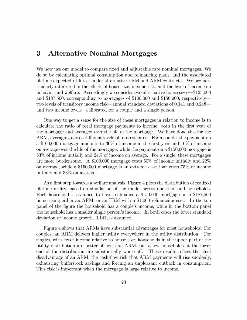
As a first step towards a welfare analysis, Figure 4 plots the distribution of realizedlifetime utility, based on simulation of the model across one thousand households.Each household is assumed to have to finance a $150,000 mortgage on a $187,500home using either an ARM, or an FRM with a $1,000 refinancing cost. In the toppanel of the figure the household has a couple’s income, while in the bottom panelthe household has a smaller single person’s income. In both cases the lower standarddeviation of income growth, 0.141, is assumed.

Figure 4 shows that ARMs have substantial advantages for most households. Forcouples, an ARM delivers higher utility everywhere in the utility distribution. Forsingles, with lower income relative to house size, households in the upper part of theutility distribution are better off with an ARM, but a few households at the lowerend of the distribution are substantially worse off. These results reflect the chiefdisadvantage of an ARM, the cash-flow risk that ARM payments will rise suddenly,exhausting bufferstock savings and forcing an unpleasant cutback in consumption.This risk is important when the mortgage is large relative to income.

23

Default

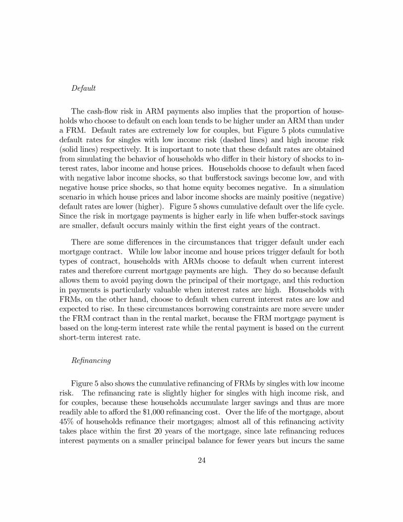
The cash-flow risk in ARM payments also implies that the proportion of house-holds who choose to default on each loan tends to be higher under an ARM than undera FRM. Default rates are extremely low for couples, but Figure 5 plots cumulativedefault rates for singles with low income risk (dashed lines) and high income risk(solid lines) respectively. It is important to note that these default rates are obtainedfrom simulating the behavior of households who differ in their history of shocks to in-terest rates, labor income and house prices. Households choose to default when facedwith negative labor income shocks, so that bufferstock savings become low, and withnegative house price shocks, so that home equity becomes negative. In a simulationscenario in which house prices and labor income shocks are mainly positive (negative)default rates are lower (higher). Figure 5 shows cumulative default over the life cycle.Since the risk in mortgage payments is higher early in life when buffer-stock savingsare smaller, default occurs mainly within the first eight years of the contract.

There are some differences in the circumstances that trigger default under eachmortgage contract. While low labor income and house prices trigger default for bothtypes of contract, households with ARMs choose to default when current interestrates and therefore current mortgage payments are high. They do so because defaultallows them to avoid paying down the principal of their mortgage, and this reductionin payments is particularly valuable when interest rates are high. Households withFRMs, on the other hand, choose to default when current interest rates are low andexpected to rise. In these circumstances borrowing constraints are more severe underthe FRM contract than in the rental market, because the FRM mortgage payment isbased on the long-term interest rate while the rental payment is based on the currentshort-term interest rate.

Refinancing

Figure 5 also shows the cumulative refinancing of FRMs by singles with low incomerisk. The refinancing rate is slightly higher for singles with high income risk, andfor couples, because these households accumulate larger savings and thus are morereadily able to afford the $1,000 refinancing cost. Over the life of the mortgage, about45% of households refinance their mortgages; almost all of this refinancing activitytakes place within the first 20 years of the mortgage, since late refinancing reducesinterest payments on a smaller principal balance for fewer years but incurs the same

24

fixed cost as early refinancing. The timing of refinancing is somewhat sensitive tothe constraint we have imposed, that homeowners must have positive home equity inorder to refinance. If we relax this constraint we get higher refinancing in the veryearly years of the mortgage, but the difference diminishes over time and is only about1% after 12 years. This reflects the fact that house prices increase on average, whileoutstanding mortgage principal diminishes, so that very few households are likely tohave persistently negative home equity.

Consumption behavior

Table 2 reports the average consumption growth rate and the standard deviationof consumption growth for households with ARMs, nominal FRMs that allow refi-nancing, and nominal FRMs without a refinancing option. The top panel of the tableis for a couple, while the bottom panel is for a single. Within each panel, we considera small or large house, and low or high income risk. Average consumption growthrates are very similar for all mortgages, since they depend largely on the hump-shapedprofile of labor income in the presence of borrowing constraints. In one case witha large house relative to income the average consumption growth rate is higher foran ARM, reflecting precautionary savings to guard against the cash-flow risk of theARM. The form of the mortgage has a larger effect on the volatility of consumptiongrowth. Volatility is lowest with an ARM, higher with a refinancing FRM, and high-est with a non-refinanceable FRM. These numbers reflect the dominance of wealthrisk over income risk in determining consumption volatility over the life cycle.

Welfare analysis

Table 3 summarizes the welfare implications of these numbers. The table reportsthe welfare provided by a FRM, with or without a refinancing option, relative to anARM. We calculate welfare using a standard consumption-equivalent methodology.For each mortgage contract we compute the constant consumption stream that makesthe household as well off in expected utility terms, and then measure the change inthis equivalent consumption stream across mortgage contracts. In all the cases weconsider, the ARM is the best available mortgage contract. The welfare consequencesof this can be very large, reflecting the importance of the mortgage decision in thefinancial life of a household. If we consider a couple with low income risk and a large$187,500 house as a benchmark case, the couple is 5.96% worse off with a nominal

25

FRM that allows cheap refinancing, and 6.79% worse off with a FRM that prohibitsrefinancing.

The welfare advantage of the ARM diminishes when the house is large relative toincome and when income is volatile. In the extreme case of a single with high incomerisk and a large house, the household is only 1.03% worse off with a refinanceableFRM than with an ARM. This reflects the fact that the cash-flow risk of an ARM isdisproportionately more important when labor income is risky and the house is largerelative to income.

By comparing welfare levels across FRMs with alternative refinancing costs, wecan obtain the value of the option to refinance. In the benchmark case this optionis worth 0.83% of consumption; it becomes more valuable when the house is largerelative to income, and when income is risky. Note that these numbers assume afixed FRM rate even while changing the cost of refinancing, and thus they do notimpose a zero-profit condition on mortgage lenders.

All the numbers in Table 3 are averages across states of the world with high andlow interest rates. We have also calculated expected utility conditional on an initialinterest rate. As one would expect, the ARM is even more advantageous if theinterest rate is initially low, since in this case the ARM has a lower cost in the earlyyears when borrowing constraints are most severe. The FRM is more attractive if theinterest rate is initially high; in the benchmark case a couple will slightly prefer anARM even with a high initial interest rate, but a single will strongly prefer a FRM.Thus our model implies that households’ financing decisions should be sensitive tothe slope of the term structure. As we discussed in the introduction, the time-seriesbehavior of US mortgage financing does not match this prediction. However ourability to explore this issue is limited by the fact that our discretized model allowsonly two possible levels of interest rates.

Bank profits

Using (16) we have calculated the average annual profit of lenders of funds undereach mortgage contract, assuming that the bank borrows funds at the one-periodriskless interest rate. In the benchmark case of a couple with low income risk and alarge house, the average annual profit is $745 for the ARM and $1218 for a refinance-able FRM. The higher average profit on the FRM comes from the term premiumthat banks earn by borrowing short and lending long; of course, this term premium

26

can be regarded as compensation for the risk that banks take when they mismatchthe maturity of their borrowing and lending.

27

4 Inflation-Indexed Mortgages

In this section we investigate the welfare properties of inflation-indexed mortgages. Inprinciple an inflation-indexed FRM can offer the wealth stability of an ARM, togetherwith the income stability of an FRM; it should therefore be a superior vehicle forhousehold risk management.

We consider inflation-indexed FRM contracts in which the interest rate is fixedin real terms. We study the welfare properties of a standard inflation-indexed FRMcontract, with constant real mortgage payments, and also those of an inflation-indexedmortgage whose real payments diminish at the average rate of inflation. We do sobecause our investor is borrowing constrained; one of the advantages of the standardinflation-indexed FRM contract, relative to the nominal FRM and ARM contracts, isthat real payments are lower early in life, when borrowing constraints are more severe.This advantage of the standard inflation-indexed contract is conceptually distinctfrom the risksharing advantage of indexation. Thus, to obtain a pure measure of therisksharing advantage of indexation we consider an inflation-indexed mortgage whosereal payments diminish at the average rate of inflation.

Inflation-indexed mortgage terms

If in period one household j chooses an inflation-indexed FRM with fixed realpayments, and the current real interest rate on an inflation-indexed FRM contractwith maturity T is RIT1, then in each subsequent period the household must make areal mortgage payment, M I

jt, of:

M Ijt =

(1− λ)PHj1HjPTj=1(1 +R

IT,1)

−j . (22)

Real mortgage payments are fixed at mortgage initiation, and nominal paymentsincrease in proportion to the price level Pt. Thus, unlike a nominal FRM, the realcapital value of an inflation-indexed mortgage is not sensitive to inflation.

For the inflation-indexed mortgage contract we ignore the possibility of refinanc-ing. Given our assumption that real interest rate variation is transitory, the gainsfrom refinancing in our model would be fairly small, and even a small monetary refi-nancing cost would prevent households from exercising their option. In reality, even

28

with persistent real interest rates, the possibility of refinancing an inflation-indexedcontract is likely to be only a minor feature of the contract, given the low volatilityof the real interest rate compared with that of nominal yields.

We assume that the date t real interest rate on an inflation-indexed FRM is givenby:

RIT−t+1,t = RT−t+1,t + θI , (23)

where θI is a constant mortgage premium over the yield on a (T − t+ 1)-period realbond, RT−t+1,t, which is determined by the expectations theory of the term structureapplied to log real interest rates. We assume that there is no log term premiumfor long-term real bonds, that is, that the real term structure is flat on average.This is consistent with the observed behavior of real yields on Treasury inflation-protected securities since their issue in 1997 (Roll 2003). Since we do not allow forthe possibility of refinancing the inflation-indexed FRM contract we set θI equal tothe ARM premium of 1.7%. This premium compensates the mortgage lender for theinitiation cost of the mortgage and for default risk.

In the inflation-indexed mortgage with real payments which diminish at the aver-age rate of inflation we have that:

MDjt =

MDj,t−1

1 + µ, (24)

whereMDt is the date t real mortgage payment and µ is average inflation. The interest

rate or internal rate of return for this mortgage contract is assumed to be equal tothat for the standard inflation-indexed FRM.

Consumption behavior, default, and bank profits

The standard inflation-indexed mortgage with constant real payments eases thehousehold’s borrowing constraints. The real payments under this contract are lowerthan the required real payments on nominal mortgages early in life, when borrowingconstraints are more severe. A measure of the degree to which investors are borrowingconstrained is consumption growth. Table 4 shows that in the benchmark case theaverage consumption growth rate under the inflation-indexed contract with constant

29

real payments is only 0.8% compared to 2.0% with an ARM or a nominal FRM.Because the inflation-indexed mortgage allows households to remain in debt later inlife, it increases the effect of income risk on consumption; thus the standard deviationof consumption growth is actually higher with this contract than with an ARM.

The inflation-indexed mortgage with declining real payments has a much smallereffect on average consumption growth. There is some reduction in the averageconsumption growth rate for households with high income risk and large houses,reflecting the fact that known real mortgage payments require smaller bufferstocks andgenerate less precautionary saving than the random real payments required by ARMs.The major effect of an inflation-indexed mortgage with declining real payments is toreduce the volatility of consumption growth, since this mortgage eliminates both thewealth risk of the nominal FRM and the income risk of the ARM.

The inflation-indexed FRM also reduces default risk. For the parameter values wehave considered, households with inflation-indexed mortgages never default. Averageannual profits of lenders are $1081 for the standard inflation-indexed mortgage, and$971 for the mortgage with declining real payments. These profits are higher thanthose for the ARM. In equilibrium these lower default rates and higher profits mightbe translated into lower inflation-indexed mortgage premiums, which would furtherbenefit households.

Welfare analysis

Figure 4 plots the distribution of realized lifetime utility for households withinflation-indexed FRMs with constant or declining real payments. The figure showsthat the welfare gains of inflation-indexed mortgages are substantial for both cou-ples and singles. The gains are particularly large for households at the bottom ofthe welfare distribution, but there are benefits to households across the distribution.The inflation-indexed mortgage with constant real payments is always superior to themortgage with declining real payments.

Table 5 shows the average welfare gains of the inflation-indexed mortgages relativeto the ARM in the form of standard consumption-equivalent variations. For ease ofreference the earlier comparison of the nominal FRM with the ARM is repeated here.In the benchmark case of a couple with a $187,500 house and low income risk, theinflation-indexed mortgage with constant real payments offers a welfare gain over anARM equivalent to 3.95% of consumption. The welfare gain increases with house

30

size and with income risk, since ARMs are particularly problematic with large housesand risky income. In the extreme case of a single with a large house and high incomerisk, the welfare gain of inflation indexation exceeds 36% of consumption.

Comparing the two inflation-indexed contracts, we see that the average welfaregains of the contract with declining real mortgage payments are considerably smallerthan those of the mortgage contract with fixed real payments, but they remain positivein every case we consider. In the benchmark case Table 5 shows that householdsare on average 0.91% better off with a declining inflation-indexed FRM than with anARM. Again the welfare gains increase dramatically with house size and income risk.

These results imply that with substantial inflation risk of the sort we have esti-mated for the 1962—1999 period, the risksharing advantages of indexation are verylarge. Households would be able to manage their lifetime risks much more effectivelyif they had access to inflation-indexed mortgage contracts. Of course, these resultsdepend on the parameters we have estimated. In the next section we assess the ben-efits of mortgage indexation for alternative parameterizations, including an incomeprocess in which nominal wages are temporarily sticky, and an interest-rate processcharacteristic of the US in the recent period of declining inflation.

31

5 Alternative Parameterizations

Sticky nominal wages

When nominal wages are inflation-indexed, or equivalently when wages are fixedin real terms, the correlation between real labor income shocks and inflation shocksis zero. We have assumed this in our benchmark parameterization. However, in aworld where implicit contracts tend to fix nominal, but not real wages, the correlationbetween inflation shocks and real labor income shocks is negative. In such a worldhouseholds may demand nominal mortgage contracts because their wage contractsare nominal. To explore this coordination feature of nominal contracts we computethe welfare benefits of inflation-indexed mortgages when nominal wages are sticky.

Table 6 repeats the welfare comparison of nominal and inflation-indexed FRMswith ARMs for several alternative specifications. We consider the benchmark caseof a couple with a large $187,500 house and low income risk. The first row ofthe table repeats the numbers from Table 5 for this case. The second row shows theaverage welfare gains of nominal and inflation-indexed FRMs for a negative correlationcoefficient of -1 between temporary real labor income shocks and inflation innovations.In the presence of negative correlation, a nominal ARM becomes much less attractivebecause positive inflation shocks drive up nominal interest rates and increase mortgagepayments at times when real labor income is temporarily low. A nominal FRMbecomes relatively more attractive, although for the benchmark case reported inTable 6 it does not dominate the ARM.

Negative correlation makes an inflation-indexed mortgage less attractive relativeto a nominal FRM. The welfare difference between the inflation-indexed FRM withdeclining real payments and the nominal FRM is 6.87% in the benchmark case witha zero correlation, but only 4.68% with a correlation of -1. However the inflation-indexed mortgage becomes more attractive relative to the ARM, which is particularlydisfavored by nominal wage stickiness.

While these results are qualitatively unsurprising, it is striking that temporarynominal wage stickiness does not reverse the welfare ordering we found in the previ-ous section, that inflation-indexed FRMs dominate ARMs, which in turn dominatenominal FRMs. To reverse that ordering we would need to assume nominal sticki-ness in the permanent component of labor income, which would imply that inflation

32

shocks permanently reduce real labor income. Such an assumption is much moreextreme than the temporary nominal stickiness we consider here.

The Volcker-Greenspan monetary policy period

Clarida, Gali, and Gertler (2000) and Campbell and Viceira (2001) report con-siderably lower inflation risk during the period since 1983 in which Federal ReserveChairmen Paul Volcker and Alan Greenspan have brought US inflation under control.We now assess the benefits of mortgage indexation when we calibrate our interest-rateprocess to a process characteristic of the US in the 1983-1999 period. For this periodwe find lower average inflation (3.4% as compared with 4.6%), less volatile inflation (astandard deviation of 1.2% as compared with 3.9%), less persistent inflation (an au-toregressive parameter of 0.41 as compared with 0.75), a higher average real interestrate (3.1% as compared with 2.0%), and a less volatile real interest rate (a standarddeviation of 1.6% as compared with 2.2%).

The third row of Table 6 changes the interest-rate parameters to those we calibratefor the 1983-1999 period. The first column shows that nominal FRMs are lessattractive relative to ARMs than was the case in our benchmark model. Evidentlythe stabilization of inflation and interest rates has reduced the income risk of ARMsrelatively more than the wealth risk of FRMs. The second and third columns showthat inflation-indexed FRMs remain superior mortgage contracts, but the welfaregain is extremely small for the inflation-indexed FRM with declining real payments.It appears that the Volcker-Greenspan monetary policy has reduced the pure riskmanagement advantages of inflation-indexed bonds to a low level.

Second loans

We now study how allowing homeowners to take out second loans, if they havepositive home equity, affects the benefits of mortgage indexation. The fourth row ofTable 6 shows the welfare gains for a second loan premium, θB, of 1% in annual terms.For tractability, in this case we eliminate the prepayment option on the nominal FRM.We see that the benefits of constant real payments are smaller when second loans areallowed, since these loans are an alternative way to relax the household’s borrowingconstraints. However second loans do not entirely eliminate the income risk of ARMs,because low house prices may coincide with low income and high inflation, in which

33

case second loans are unavailable precisely when they would be most valuable. Thusour basic results survive the addition of second loans to our model.

Moving probability

We have also solved our model assuming a moving probability equal to 0.10,meaning that the household moves on average once every ten years. Recall that inall the cases reported in earlier tables, the probability of moving is equal to zero.We find that the welfare gain of an ARM over a nominal FRM is higher when themoving probability is higher. If a homeowner knows he is highly likely to move in thenear future, he is more likely to use the kind of mortgage that has the lower currentinterest rate. On average, this is the ARM or the inflation-indexed FRM since thenominal FRM has a higher yield spread that reflects the slope of the nominal termstructure.

Consumption in default

Our results are sensitive to the assumption that we make about consumption inthe event of a mortgage default. In the model we assume that in case of defaultthe bank seizes the house and the household is forced into the rental market for theremainder of its life. We set the rental premium equal to the user cost of housing plusa constant rental premium, θR, which in the benchmark parameterization is equalto 3%. The sixth and seventh rows of Table 6 consider lower and a higher valuesfor the rental premium of 2% and 4% respectively. We interpret these as roughlycapturing the effects of different default costs or exemption levels in the event ofpersonal bankruptcy. From Table 6 we see that cheaper default makes a nominalFRM less attractive relative to an ARM, because it mitigates the income risk of theARM. The benefits of FRM indexation are also reduced but remain substantial.Naturally, the cheaper is default the higher is the default rate.

These results suggest that in states or countries where bankruptcy is relativelycheaper one should observe, ceteris paribus, a higher proportion of households choos-ing ARMs. However we do not adjust the ARM premium θA to compensate lendersfor variations in the default rate caused by variations in the rental premium, and thusour results do not capture the full general equilibrium effect of the bankruptcy code.

34

Impatient and risk-averse households

In the eighth row of Table 6 we consider impatient investors with a higher timediscount rate and a correspondingly smaller time discount factor of 0.90. Suchinvestors accumulate a smaller buffer-stock of liquid financial assets, so they defaultmore often and are more affected by the wealth risk of nominal FRMs and the incomerisk of ARMs. They gain more from inflation-indexation, even if real paymentsdecline over time. They particularly benefit from the postponed payments of aninflation-indexed FRM with constant real payments.

In the ninth row of the table, we increase the risk aversion coefficient from 3 to 5.This causes households to become more concerned about the income risk of ARMs.The welfare advantage of ARMs over nominal FRMs diminishes, and the benefits ofinflation-indexation increase. Much of the gain from inflation—indexation comes fromimproved risk management, but these households also have a strong preference forsmooth consumption so they benefit from declining real mortgage payments.

Higher standard deviation of persistent income shocks

The tenth row of Table 6 shows the results for a higher standard deviation ofpermanent income shocks equal to 5%. The results are qualitatively similar to thosefor the benchmark case. The main quantitative difference is a reduced benefit of aninflation-indexed mortgage with constant real payments. This change is explainedby the fact that with risky permanent income, the option to default becomes morevaluable for the ARM and nominal FRM contracts relative to the inflation-indexedmortgage with constant real payments. Once again we do not adjust the ARM orFRM premium for variations in default caused by the change in the volatility of in-come, and thus our results reflect only a partial equilibrium, not a general equilibriumanalysis.

ARM cap and floor

In the eleventh row of Table 6 we consider a hybrid ARM in which there is a capof 2% on the annual increase in the interest rate, and a lifetime cap of 6% on thecumulative interest rate increase after mortgage initiation. These terms are fairly

35

standard ones for a hybrid ARM. The hybrid ARM is more attractive than eithera straight ARM or a nominal FRM, as it mitigates income risk while still limitingwealth risk. The benefits of mortgage indexation are smaller in comparison to ahybrid ARM, and shrink to 7 basis points for an inflation-indexed mortgage withdeclining real payments.

In practice, ARMs often have more complicated terms including a low initial teaserrate. A teaser rate enables an ARM to capture some of the benefits of an inflation-indexed mortgage with constant real payments, but we do not attempt to capture thefull richness of available ARM contracts here.

Correlation of income and interest rates

Our benchmark model assumes that shocks to income growth are uncorrelatedwith shocks to real interest rates. If we assume instead that income growth isnegatively correlated with real interest rates, this exacerbates the income risk ofARMs, since income will tend to be low precisely when interest rates are high andrequired ARM mortgage payments are high. The twelfth row of Table 6 showsthat with a correlation of -0.2 between income and real interest rates, nominal andinflation-indexed FRMs become slightly more attractive relative to ARMs.

Term premium in the real term structure

The last row of Table 6 assumes that the term premium ξ of 1% applies to the realterm structure as well as the nominal term structure. In this case the spread betweenlong-term nominal and real interest rates is caused only by expected inflation and doesnot include an inflation risk premium. This increases the cost of an inflation-indexedmortgage relative to a nominal mortgage, and reduces the benefit of indexation.Under this assumption an ARM looks attractive as a way for a homeowner to avoidpaying the term premium.

Refinancing from an ARM to a FRM

Finally, we consider an alternative specification in which we allow householdswho choose a nominal ARM to subsequently refinance into a nominal FRM. Recall

36

that our baseline specification compares a nominal ARM to a nominal FRM, withoutallowing households to switch between the two. In practice, and even though thereare transaction costs associated with switching between different types of mortgages,it is possible to do so. The complexity of our model prevents us from considering aperiod-by-period decision to switch mortgages. However, we can study the welfareeffects of allowing a one time switch from a nominal ARM to a nominal FRM. It maybe the case that ARM borrowers find it optimal to choose the ARM when interestrates are low, but plan to switch to a FRM if and when interest rates increase.

The solution to this alternative specification requires that at each date t andfor each combination of the state variables, we compare the utility of remaining anARM borrower to the utility of switching to the FRM contract. More precisely, letVt(Xt;FRM) denote the lifetime utility of becoming an FRMborrower at date t, whenthe vector of state variables is given byXt. Assuming a zero switching cost, the house-hold will at date t switch to the FRM if and only if Vt(Xt;FRM) > Vt(Xt;ARM),where Vt(Xt;ARM) is the lifetime utility of remaining an ARM borrower with theoption to switch to the FRM in a subsequent period.

To solve for the optimal mortgage choices under this alternative specification,we set the parameters equal to their benchmark values and the switching cost tozero. For these parameters most borrowers prefer an ARM and never switch to aFRM. There are 1.3% of households who start off with an ARM and later on switchto a FRM when current interest rates are high. However, not all households findit optimal to switch to the FRM when current rates are high; only those with lowcurrent income and financial wealth do so. The intuition for this result is simple: whencurrent interest rates are high the ARM implies a larger current mortgage paymentthan the FRM. Those consumers who are more borrowing constrained find it optimalto pay the higher average premium on the FRM in exchange for the lower currentmortgage payments. This result illustrates once more the importance of borrowingconstraints for mortgage choice. As consumers grow older the labor income profilebecomes flatter and households become less borrowing constrained. For this reasonthe benefits of switching to the FRM contract are lower. This explains our findingthat for the baseline parameters all the switching from the ARM to the FRM takesplace before age 38.

We also study the welfare effects of allowing consumers to switch from the ARMto the FRM. We compute the mean welfare gain delivered by the ARM with theoption to switch to the FRM, relative to the baseline nominal ARM contract. We

37

find a modest welfare gain of 0.27%, reflecting the small number of households thatchoose to make this switch.

38

6 Conclusion

The problem of mortgage choice is both basic and complex. It is basic because almostevery middle-class American faces this choice at least once in his or her life. It iscomplex because it involves many considerations that are at the frontier of financetheory: uncertainty in inflation and interest rates, borrowing constraints, illiquidassets, uninsurable risk in labor income, and the need to plan over a long horizon.

Despite the complexity of the problem, it is important for financial economists totry to offer scientifically grounded advice. If financial economists avoid the topic,homeowners may be guided by unwise commercial or journalistic advice; for examplethey may be urged to time the bond market by predicting the direction of long-terminterest rates. Mortgage choice should not be left to specialists in real estate, butshould be treated as an aspect of household risk management, a topic that lies at theheart of finance.

In this paper we have shown that the form of the mortgage contract can have largeeffects on household welfare. We begin by comparing pure forms of the standardnominal ARM and FRM contracts. FRM contracts expose households to wealthrisk, while ARM contracts expose them to income risk: the risk that borrowingconstraints will bind more severely when high interest rates coincide with low incomeand house prices. While the exact levels of welfare depend on the particular premiawe have assumed for ARM and FRM mortgages, we can draw general conclusionsabout the types of households that should be more likely to use ARMs. Householdswith smaller houses relative to income, more stable income, lower risk aversion, morelenient treatment in bankruptcy, and a higher probability of moving should be thehouseholds that find ARMs most attractive.

Interestingly, these results match quite well with empirical evidence reported byShilling, Dhillon, and Sirmans (1987). These authors look at micro data on mortgageborrowing and estimate a reduced-form econometric model of mortgage choice. Theyfind that households with co-borrowers and married couples (whose household incomeis presumably more stable) and households with a higher moving probability are morelikely to use ARMs.

We have also investigated the welfare properties of innovative inflation-indexedmortgage contracts. An inflation-indexed FRM can offer the wealth stability of anARM together with the income stability of an FRM, so it is a superior vehicle for

39

household risk management. Using US data from the period 1962—1999 we find verylarge welfare gains from the availability of an inflation-indexed mortgage contract.Some of these gains arise from the reduced mortgage payments early in the life ofthe mortgage that are implied by a constant real payment as opposed to a constantnominal payment. Even if we remove this advantage by requiring real payments thatdecline at the expected rate of inflation, we still find substantial welfare gains fromindexation.

This finding raises the question of why inflation-indexed mortgages are not morecommonly used. There are several possible answers to this question. First, the yieldspreads between inflation-indexed Treasury securities and nominal Treasury securi-ties have been extremely low, generally below 2%, since inflation-indexed Treasurysecurities were introduced in 1997 (Roll 2003). This suggests that investors have ahigh degree of confidence that inflation will remain low in the future, and that theinflation risk premium is low. When we calibrate our interest-rate model to theperiod since 1983 in which inflation has been relatively well controlled, or when weassume a zero inflation risk premium, we find smaller risk management benefits ofindexation. Second, we find that hybrid ARMs with nominal interest rate caps canimprove significantly over pure ARMs. These ARMs reduce the benefits of inflation-indexation.

Third, inflation-indexed mortgages can cause the outstanding principal of themortgage to increase over time in nominal terms (although not in real terms). Finan-cial advisers frequently warn against such “negative amortization”, without makingany distinction between real and nominal debt. Irwin (1996), for example, writes“Another trap has to do with negative amortization. Some of the adjustable loanskeep the monthly payments down by adding the interest to the principal. In otherwords, you end up owing more than you borrowed!” Even more colorfully, Tysonand Brown (2000) write “Negative amortization has the potential to be a personalfinancial neutron bomb. It destroys the borrower without harming the property. Ifyou’re offered an ARM with negative amortization, emphatically say NO!”11 Suspi-cion of negative amortization may have inhibited acceptance of innovative mortgagecontracts that might reduce the income risk of standard ARMs.

Although our model captures many of the important factors that should influence11Steinmetz (2002) offers a more nuanced view, stating that “Negative amortization is not inher-

ently bad”. However he, like the other authors quoted here, does not try to distinguish the realvalue of a debt from its nominal value.

40

mortgage choice, it remains oversimplified in several important respects. First, wehave assumed that households remain in a house of fixed size unless they are ran-domly forced to move, in which case we evaluate their welfare using a terminal utilityfunction. Second, related to this we assume a relatively low volatility of permanentincome growth in order to avoid large mismatches between household income andhouse size. Third, our model is too stylized to capture teaser rates and other specialfeatures of many mortgages that are offered in the marketplace. Fourth, we workin partial equilibrium and do not attempt to use zero-profit conditions for mortgagelenders to solve for equilibriummortgage premia. We believe there is room for furtherresearch to model these issues in a more satisfactory manner.

We have calibrated our model to match basic features of the US mortgage mar-ket. Other countries have mortgage markets that differ in important respects. Forexample, long-term nominal fixed-rate mortgages are almost unknown in the UK andCanada. An interesting area for future research will be to relate these internationaldifferences in prevailing mortgage contracts to differences in the risk managementproblem that households face.

The concept of income risk that we emphasize in this paper has interesting im-plications for other areas of finance. Corporations, for example, must consider therisk that short-term or floating-rate debt will require high interest payments in cir-cumstances where internal cash flow and collateral are low and external financing isexpensive. Here as in the problem of mortgage choice, borrowing constraints bothcomplicate and enrich standard models of risk management.

41

References

Abowd, J. and Card, D., 1989, “On the Covariance Structure of Earnings and HoursChanges,” Econometrica 57, 411—445.

Alm, J. and Follain, J. R., 1984, “Alternative Mortgage Instruments, the Tilt Prob-lem and Consumer Welfare,” Journal of Financial and Quantitative Analysis19, 113—126.

Black, Deborah G., Kenneth D. Garbade, and William L. Silber, 1981, “The Impactof the GNMA Pass-Through Program on FHA Mortgage Costs”, Journal ofFinance 36, 457—469.

Brueckner, J. , 1993, “Why Do We Have ARMs,” American Real Estate and UrbanEconomic Associations Journal 21, 333—345.

Brueckner, J., 1994, “Borrower Mobility, Adverse Selection and Mortgage Points,”Journal of Financial Intermediation 3, 416—441.

Brueckner, J., and J.R. Follain, 1988, “The Rise and Fall of the ARM: An Econo-metric Analysis of Mortgage Choice,” Review of Economics and Statistics 70,93—102.

Campbell, John Y. and John Ammer, 1993, “What Moves the Stock and BondMarkets? A Variance Decomposition for Long-Term Asset Returns”, Journalof Finance 48, 3—37.

Campbell, John Y., Andrew W. Lo, and A. Craig MacKinlay, 1997, The Economet-rics of Financial Markets, Princeton University Press, Princeton, NJ.

Campbell, John Y. and Robert J. Shiller, 1991, “Yield Spreads and Interest RateMovements: A Bird’s Eye View”, Review of Economic Studies 58, 495—514.

Campbell, John Y. and Robert J. Shiller, 1996, “A Scorecard for Indexed Govern-ment Debt”, in Ben S. Bernanke and Julio J. Rotemberg eds. NBER Macro-economics Annual 1996, 155—197, MIT Press, Cambridge, MA.

Campbell, John Y. and Luis M. Viceira, 2001, “Who Should Buy Long-TermBonds?”,American Economic Review 91, 99—127.

42

Campbell, John Y. and Luis M. Viceira, 2002, Strategic Asset Allocation: PortfolioChoice for Long-Term Investors, Oxford University Press, Oxford.

Caplin, Andrew S., Sewin Chan, Charles Freeman, and Joseph Tracy, 1997, Hous-ing Partnerships: A New Approach to a Market at a Crossroads, MIT Press,Cambridge, MA.

Caplin, Andrew S., Charles Freeman, and Joseph Tracy, 1997, “Collateral Damage:Refinancing Constraints and Regional Recessions”, Journal of Money, Credit,and Banking 29, 496—516.

Carroll, Christopher D., 1992, “The Buffer-Stock Theory of Saving: Some Macro-economic Evidence”, Brookings Papers on Economic Activity, 61—156.

Carroll, Christopher D., 1997, “Buffer-Stock Saving and the Life-Cycle/PermanentIncome Hypothesis”, Quarterly Journal of Economics 114, 433—495.

Carroll, Christopher D. and Andrew A. Samwick, 1997, “The Nature of Precaution-ary Wealth”, Journal of Monetary Economics 40, 41—71.

Case, Karl E. and Robert J. Shiller, 1989, “The Efficiency of the Market for Single-Family Homes,” American Economic Review, 79, 125—137.

Chan, Sewin, 2001, “Spatial Lock-in: Do Falling House Prices Constrain ResidentialMobility?”, Journal of Urban Economics 49, 567—586.

Chari, V.V. and Ravi Jagannathan, 1989, “Adverse Selection in a Model of RealEstate Lending,” Journal of Finance 44, 499—508.

Clarida, Richard, Jordi Gali, and Mark Gertler, 2000, “Monetary Policy Rules andMacroeconomic Stability: Evidence and Some Theory”, Quarterly Journal ofEconomics 115, 147—180.

Cocco, João F., 2001, “Portfolio Choice in the Presence of Housing”, unpublishedpaper, London Business School.

Cocco, João F., Francisco J. Gomes, and Pascal J. Maenhout, 1999, “Consumptionand Portfolio Choice over the Life-Cycle”, unpublished paper, London BusinessSchool and Harvard University.

43

Cotterman, Robert F. and James E. Pearce, 1996, “The Effects of the Federal Na-tional Mortgage Association and the Federal Home Loan Mortgage Corporationon Conventional Fixed-Rate Mortgage Yields”, in Studies on Privatizing FannieMae and Freddie Mac, U.S. Department of Housing and Urban Development,Office of Policy Development and Research.

Davidoff, Thomas, 2002, “Labor Income, Housing Prices, and Homeownership”,unpublished paper, Haas School of Business, UC Berkeley.

Deaton, Angus S., 1991, “Savings and Liquidity Constraints,” Econometrica 59,1221—1248.

Dunn, Kenneth B. and Chester S. Spatt, 1985, “An Analysis of Mortgage Contract-ing: Prepayment Penalties and the Due-on-Sale Clause,” Journal of Finance40, 293—308.

Fabozzi, Frank J. and Franco Modigliani, 1992, Mortgage and Mortgage-BackedSecurities Markets, Harvard Business School Press, Boston, MA.

Fama, Eugene F., 1975, “Short-Term Interest Rates as Predictors of Inflation”,American Economic Review 65, 269—282.

Fama, Eugene F., 1990, “Term Structure Forecasts of Interest Rates, Inflation, andReal Returns”, Journal of Monetary Economics 25, 59—76.

Fisher, Sarah and Susan Shelly, 2002, The Complete Idiot’s Guide to Personal Fi-nance in Your 20’s and 30’s, 2nd ed., Alpha Books, Indianapolis, IN.

Flavin, Marjorie and Takashi Yamashita, 2002, “Owner-Occupied Housing and theComposition of the Household Portfolio”, American Economic Review 92, 345—362..

Follain, J. R., 1990, “Mortgage Choice,” American Real Estate and Urban EconomicAssociations Journal 18, 125—144.

Fratantoni, Michael C., 2001, “Homeownership, Committed Expenditure Risk, andthe Stockholding Puzzle”, Oxford Economic Papers 53, 241—259.

Garcia, René and Pierre Perron, 1996, “An Analysis of the Real Interest Rate underRegime Shifts”, Review of Economics and Statistics 78, 111—125.

44

Goetzmann, William N., 1993, “The Single Family Home in the Investment Portfo-lio”, Journal of Real Estate Finance and Economics 6, 201—222.

Gottschalk, Peter, and Robert Moffitt, 1994, “The Growth of Earnings Instabilityin the U.S. Labor Market”, Brookings Papers on Economic Activity 2, 217—272.

Gourinchas, Pierre-Olivier and Jonathan Parker, 2002, “Consumption Over the LifeCycle”, Econometrica 70, 47—89.

Gray, Stephen F., 1996, “Modelling the Conditional Distribution of Interest Ratesas a Regime-Switching Process”, Journal of Financial Economics 42, 27—62.

Hu, Xiaoqing, 2001, “Portfolio Choices for Home Owners”, unpublished paper,Northwestern University.

Irwin, Robert, 1996, Tips and Traps When Buying a Home, 2nd ed., McGraw-Hill,New York, NY.

Irwin, Robert, 1999, Tips and Traps When Mortgage Hunting, 2nd ed., McGraw-Hill,New York, NY.

Kearl, J.R., 1979, “Inflation, Mortgages, and Housing”, Journal of Political Economy87, 1115—1138.

LeRoy, Stephen F., 1996, “Mortgage Valuation Under Optimal Prepayment,” Reviewof Financial Studies 9, 817—844.

MaCurdy, Thomas, 1982, “The Use of Time Series Processes to Model The ErrorStructure of Earnings in a Longitudinal Data Analysis”, Journal of Economet-rics 18, 83—114.

Merton, Robert C., 1973, “An Intertemporal Capital Asset Pricing Model”, Econo-metrica 41, 867—887.

Mishkin, Frederic S., 1990, “What Does the Term Structure Tell Us About FutureInflation?”, Journal of Monetary Economics 25, 77—95.

Orman, Suze, 1999, The Courage to Be Rich, Riverhead Books, New York, NY.

Ortalo-Magné, François and Sven Rady, 2001, “Housing Market Dynamics: On theContribution of Income Shocks and Credit Constraints,” unpublished paper,LSE.

45

Poterba, James M., 1991, “House Price Dynamics: The Role of Tax Policy andDemography,” Brookings Papers on Economic Activity 2, 143—183.

Roll, Richard, 2003, “Empirical TIPs”, unpublished paper, Anderson GraduateSchool of Management, UCLA.

Rothberg, James P., Frank E. Nothaft, and Stuart A. Gabriel, 1989, “On the De-terminants of Yield Spreads Between Mortgage Pass-Through and TreasurySecurities”, Journal of Real Estate Finance and Economics 2, 301—315.

Schwartz, Eduardo S. and Walter N. Torous, 1989, “Prepayment and the Valuationof Mortgage-Backed Securities”, Journal of Finance 44, 375—392.

Shiller, Robert J., 1998,Macro Markets: Creating Institutions for Managing Society’sLargest Economic Risks, Oxford University Press, New York, NY.

Shiller, Robert J. and Allan Weiss, 1999, “Home Equity Insurance”, Journal of RealEstate Finance and Economics 19, 21—47.

Shilling, J.D., U. S. Dhillon, and C.F. Sirmans, 1987, “Choosing Between Fixedand Adjustable Rate Mortgages,” Journal of Money, Credit, and Banking 19,260—267.

Sinai, Todd and Nicholas Souleles, 2003, “Owner-Occupied Housing as a HedgeAgainst Rent Risk”, unpublished paper, Wharton School, University of Penn-sylvania.

Skinner, Jonathan, 1994, “Housing and Saving in the United States”, in YukioNoguchi and James M. Poterba eds. Housing Markets in the United Statesand Japan, University of Chicago Press, Chicago, IL, 191—213.

Stanton, Richard, 1995, “Rational Prepayment and the Valuation of Mortgage-Backed Securities”, Review of Financial Studies 8, 677—708.

Stanton, Richard and Nancy Wallace, 1998, “Mortgage Choice: What’s the Point?”,Real Estate Economics 26, 173—205.

Stanton, Richard and Nancy Wallace, 1999, “Anatomy of an ARM: The Interest-Rate Risk of Adjustable-Rate Mortgages”, Journal of Real Estate Finance andEconomics 19, 49—67.

46

Statman, Meir, 1982, “Fixed Rate or Index-Linked Mortgages from the Borrower’sPoint of View: A Note”, Journal of Financial and Quantitative Analysis 17,451—457.

Steinmetz, Thomas C., 2002, The Mortgage Kit, 5th ed., Dearborn Trade Publishing,Chicago, IL.

Storesletten, Kjetil, Chris I. Telmer, and Amir Yaron, 2003, “Consumption and RiskSharing over the Life Cycle”, forthcoming Journal of Monetary Economics.

Tauchen, George and R. Hussey, 1991, “Quadrature-Based Methods for ObtainingApproximate Solutions to Nonlinear Asset Pricing Models”, Econometrica 59,371—396.

Tracy, Joseph and Henry Schneider, 2001, “Stocks in the Household Portfolio: ALook Back at the 1990s”, Current Issues in Economics and Finance 7(4), 1—6,Federal Reserve Bank of New York.

Tracy, Joseph, Henry Schneider, and Sewin Chan, 1999, “Are Stocks Overtaking RealEstate in Household Portfolios?”, Current Issues in Economics and Finance5(5), 1—6, Federal Reserve Bank of New York.

Tyson, Eric and Ray Brown, 2000, Mortgages for Dummies, Hungry Minds Inc.,New York, NY.

Woodward, Susan, 2001, “Rechartering Freddie and Fannie: The Policy Issues”,unpublished paper, Sand Hill Econometrics.

Yao, Rui and Harold H. Zhang, 2001, “Optimal Consumption and Portfolio Choiceswith Risky Housing and Stochastic Labor Income”, unpublished paper, Univer-sity of North Carolina at Chapel Hill.

Zeldes, Stephen, 1989, “Optimal Consumption with Stochastic Income: Deviationsfrom Certainty Equivalence”, Quarterly Journal of Economics 104, 275—298.

47

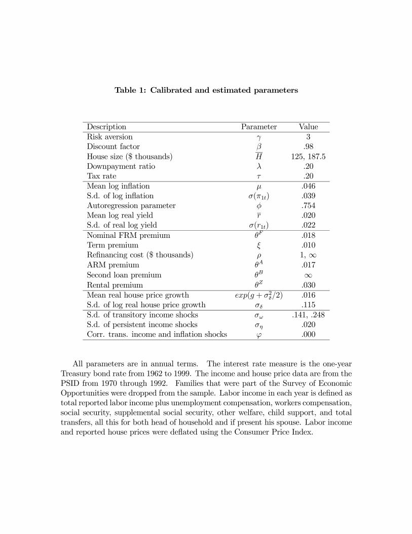
Table 1: Calibrated and estimated parameters

Description Parameter ValueRisk aversion γ 3Discount factor β .98House size ($ thousands) H 125, 187.5Downpayment ratio λ .20Tax rate τ .20Mean log inflation µ .046S.d. of log inflation σ(π1t) .039Autoregression parameter φ .754Mean log real yield r .020S.d. of real log yield σ(r1t) .022Nominal FRM premium θF .018Term premium ξ .010Refinancing cost ($ thousands) ρ 1, ∞ARM premium θA .017Second loan premium θB ∞Rental premium θZ .030Mean real house price growth exp(g + σ2δ/2) .016S.d. of log real house price growth σδ .115S.d. of transitory income shocks σω .141, .248S.d. of persistent income shocks ση .020Corr. trans. income and inflation shocks ϕ .000

All parameters are in annual terms. The interest rate measure is the one-yearTreasury bond rate from 1962 to 1999. The income and house price data are from thePSID from 1970 through 1992. Families that were part of the Survey of EconomicOpportunities were dropped from the sample. Labor income in each year is defined astotal reported labor income plus unemployment compensation, workers compensation,social security, supplemental social security, other welfare, child support, and totaltransfers, all this for both head of household and if present his spouse. Labor incomeand reported house prices were deflated using the Consumer Price Index.

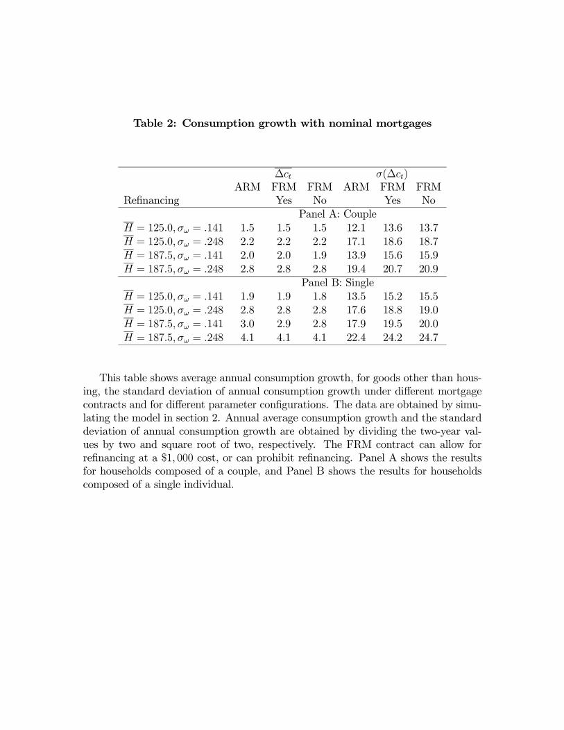
Table 2: Consumption growth with nominal mortgages

∆ct σ(∆ct)ARM FRM FRM ARM FRM FRM

Refinancing Yes No Yes NoPanel A: Couple

H = 125.0,σω = .141 1.5 1.5 1.5 12.1 13.6 13.7H = 125.0,σω = .248 2.2 2.2 2.2 17.1 18.6 18.7H = 187.5,σω = .141 2.0 2.0 1.9 13.9 15.6 15.9H = 187.5,σω = .248 2.8 2.8 2.8 19.4 20.7 20.9

Panel B: SingleH = 125.0,σω = .141 1.9 1.9 1.8 13.5 15.2 15.5H = 125.0,σω = .248 2.8 2.8 2.8 17.6 18.8 19.0H = 187.5,σω = .141 3.0 2.9 2.8 17.9 19.5 20.0H = 187.5,σω = .248 4.1 4.1 4.1 22.4 24.2 24.7

This table shows average annual consumption growth, for goods other than hous-ing, the standard deviation of annual consumption growth under different mortgagecontracts and for different parameter configurations. The data are obtained by simu-lating the model in section 2. Annual average consumption growth and the standarddeviation of annual consumption growth are obtained by dividing the two-year val-ues by two and square root of two, respectively. The FRM contract can allow forrefinancing at a $1, 000 cost, or can prohibit refinancing. Panel A shows the resultsfor households composed of a couple, and Panel B shows the results for householdscomposed of a single individual.

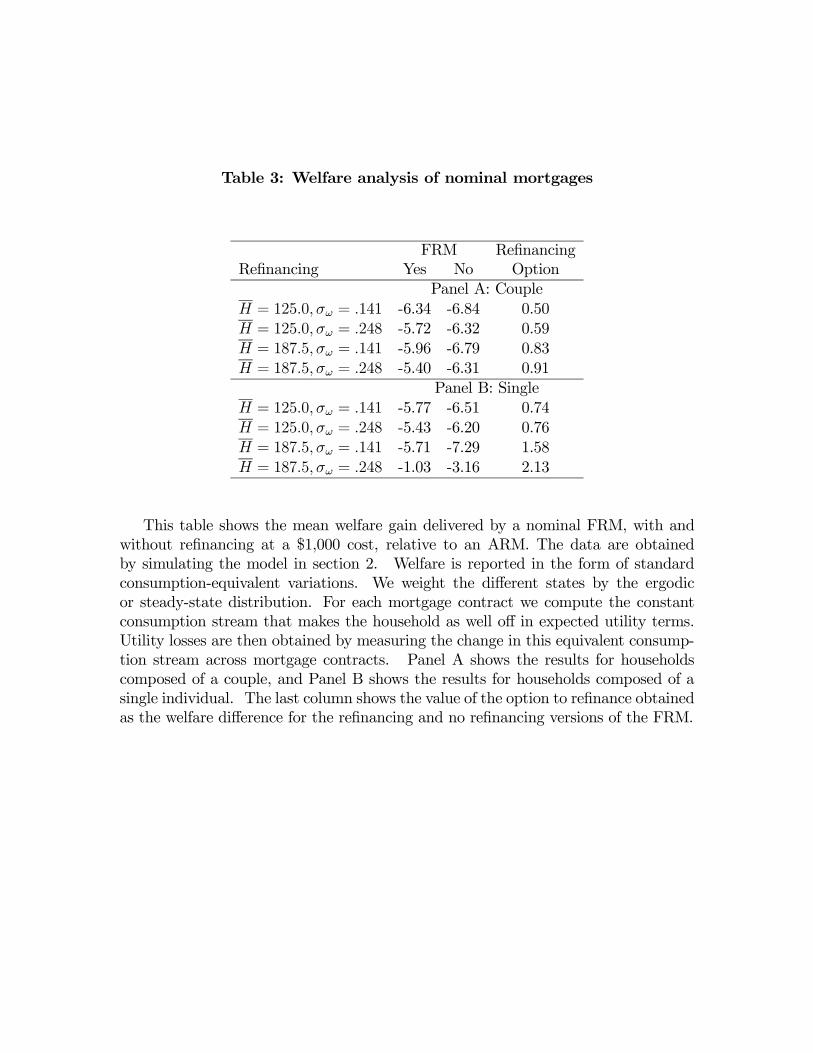
Table 3: Welfare analysis of nominal mortgages

FRM RefinancingRefinancing Yes No Option

Panel A: CoupleH = 125.0,σω = .141 -6.34 -6.84 0.50H = 125.0,σω = .248 -5.72 -6.32 0.59H = 187.5,σω = .141 -5.96 -6.79 0.83H = 187.5,σω = .248 -5.40 -6.31 0.91

Panel B: SingleH = 125.0,σω = .141 -5.77 -6.51 0.74H = 125.0,σω = .248 -5.43 -6.20 0.76H = 187.5,σω = .141 -5.71 -7.29 1.58H = 187.5,σω = .248 -1.03 -3.16 2.13

This table shows the mean welfare gain delivered by a nominal FRM, with andwithout refinancing at a $1,000 cost, relative to an ARM. The data are obtainedby simulating the model in section 2. Welfare is reported in the form of standardconsumption-equivalent variations. We weight the different states by the ergodicor steady-state distribution. For each mortgage contract we compute the constantconsumption stream that makes the household as well off in expected utility terms.Utility losses are then obtained by measuring the change in this equivalent consump-tion stream across mortgage contracts. Panel A shows the results for householdscomposed of a couple, and Panel B shows the results for households composed of asingle individual. The last column shows the value of the option to refinance obtainedas the welfare difference for the refinancing and no refinancing versions of the FRM.

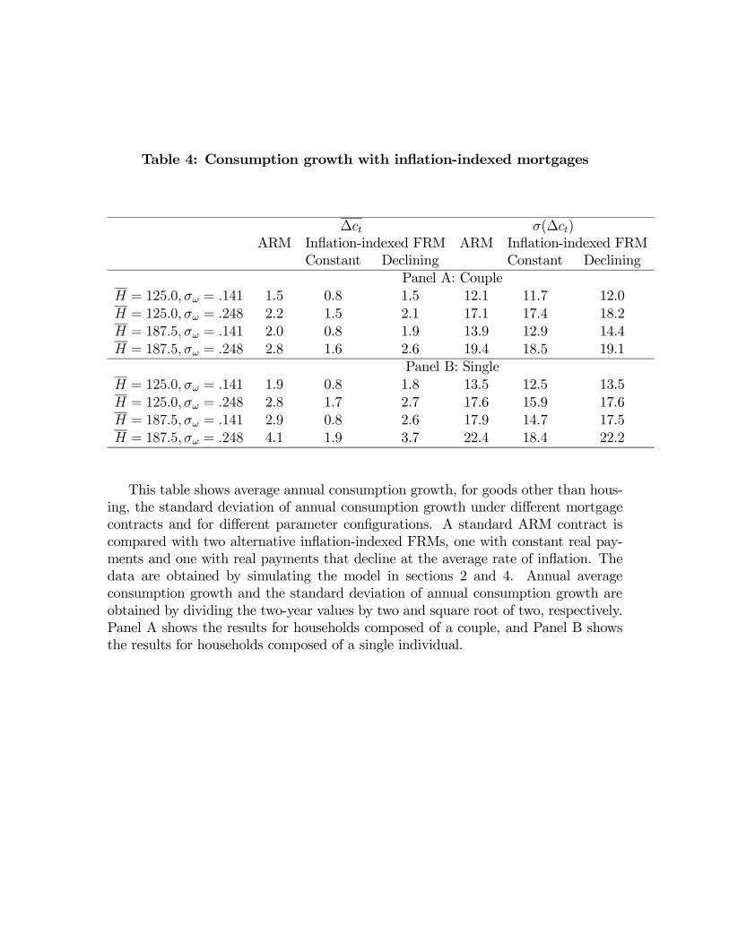
Table 4: Consumption growth with inflation-indexed mortgages

∆ct σ(∆ct)ARM Inflation-indexed FRM ARM Inflation-indexed FRM

Constant Declining Constant DecliningPanel A: Couple

H = 125.0,σω = .141 1.5 0.8 1.5 12.1 11.7 12.0H = 125.0,σω = .248 2.2 1.5 2.1 17.1 17.4 18.2H = 187.5,σω = .141 2.0 0.8 1.9 13.9 12.9 14.4H = 187.5,σω = .248 2.8 1.6 2.6 19.4 18.5 19.1

Panel B: SingleH = 125.0,σω = .141 1.9 0.8 1.8 13.5 12.5 13.5H = 125.0,σω = .248 2.8 1.7 2.7 17.6 15.9 17.6H = 187.5,σω = .141 2.9 0.8 2.6 17.9 14.7 17.5H = 187.5,σω = .248 4.1 1.9 3.7 22.4 18.4 22.2

This table shows average annual consumption growth, for goods other than hous-ing, the standard deviation of annual consumption growth under different mortgagecontracts and for different parameter configurations. A standard ARM contract iscompared with two alternative inflation-indexed FRMs, one with constant real pay-ments and one with real payments that decline at the average rate of inflation. Thedata are obtained by simulating the model in sections 2 and 4. Annual averageconsumption growth and the standard deviation of annual consumption growth areobtained by dividing the two-year values by two and square root of two, respectively.Panel A shows the results for households composed of a couple, and Panel B showsthe results for households composed of a single individual.

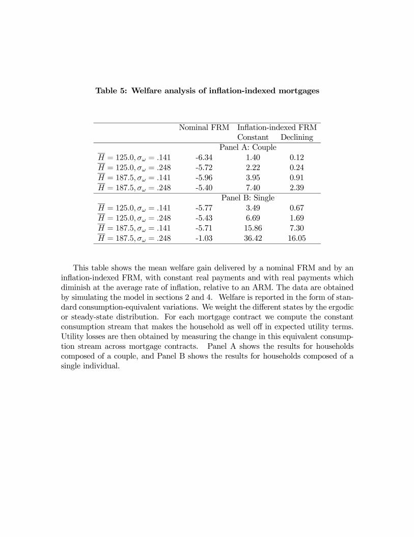
Table 5: Welfare analysis of inflation-indexed mortgages

Nominal FRM Inflation-indexed FRMConstant Declining

Panel A: CoupleH = 125.0,σω = .141 -6.34 1.40 0.12H = 125.0,σω = .248 -5.72 2.22 0.24H = 187.5,σω = .141 -5.96 3.95 0.91H = 187.5,σω = .248 -5.40 7.40 2.39

Panel B: SingleH = 125.0,σω = .141 -5.77 3.49 0.67H = 125.0,σω = .248 -5.43 6.69 1.69H = 187.5,σω = .141 -5.71 15.86 7.30H = 187.5,σω = .248 -1.03 36.42 16.05

This table shows the mean welfare gain delivered by a nominal FRM and by aninflation-indexed FRM, with constant real payments and with real payments whichdiminish at the average rate of inflation, relative to an ARM. The data are obtainedby simulating the model in sections 2 and 4. Welfare is reported in the form of stan-dard consumption-equivalent variations. We weight the different states by the ergodicor steady-state distribution. For each mortgage contract we compute the constantconsumption stream that makes the household as well off in expected utility terms.Utility losses are then obtained by measuring the change in this equivalent consump-tion stream across mortgage contracts. Panel A shows the results for householdscomposed of a couple, and Panel B shows the results for households composed of asingle individual.

Table 6: Welfare analysis under alternative parameterizations

Nominal FRM Inflation-indexed FRMConstant Declining

1. Benchmark -5.96 3.95 0.912. Correlated income and inflation (ϕ = −1.00) -2.87 5.16 1.813. 1983-1999 parameters -6.94 1.01 0.024. Lower second loan premium (θB = 1%) -6.40 1.57 0.975. Higher moving probability (p = 10%) -6.60 8.94 0.866. Lower rental premium (θZ = 2%) -6.08 3.83 0.857. Higher rental premium (θZ = 4%) -5.79 4.14 1.098. Higher time discount rate (β = 0.90) -6.49 12.46 1.469. Higher risk aversion (γ = 5) -1.33 8.12 4.5810. More volatile permanent income (ση = 5%) -5.11 2.17 0.9011. Hybrid ARM contract -6.75 3.09 0.0712. Correlated income and real rates -5.90 4.02 0.9713. Term premium in the real term structure -5.96 -1.34 -3.72

This table shows the mean welfare gain delivered by a nominal FRM and by aninflation-indexed FRM, with constant real payments and with real payments whichdiminish at the average rate of inflation, relative to an ARM for different parameteri-zations. The data are obtained by simulating the model in sections 2 and 4. The firstrow shows the results for our benchmark case, which is a couple needing to financea house of $187, 500 and facing labor income risk σω = .141. The second shows theresults for a correlation between transitory labor income and inflation shocks equal tominus one. The third row shows the results when the parameters of the inflation andreal interest rate processes are calibrated using data for the 1983-1999 period. The an-nual parameters are: µ = .034, σ(π1t) = .012, φ = .412, r = .031, and σ(r1t) = .016.In the fourth row we allow homeowners to take out second loans if they have positivehome equity, with a second loan premium of 1%. The fifth row shows the results fora probability of moving equal to 10%. The sixth and seventh rows show the resultsfor a lower and a higher rental premium in case of default. The eighth row showsthe results for a higher time discount rate, corresponding to a lower time discountfactor of 0.90. The ninth row shows the results for a higher coefficient of relativerisk aversion. The tenth row shows the results for a higher standard deviation for

permanent income shocks. The eleventh row shows the results for a hybrid ARMcharacterized by a 2% cap per year and a 6% lifetime cap. The twelfth row showsthe results for a correlation of income growth and real interest rate shocks equal to−0.2. The last row shows the results assuming that the term premium of 1% is inthe real term structure rather than the nominal term structure.

Figure 1: Portion of Household Assets in Corporate Equity and Real Estate by Wealth

Percentile, 1989 and 1998. The data are from the 1989 and 1998 Survey of Consumer

Finances. We would like to thank Joe Tracy for kindly providing us the data for this

figure.

Figure 1: Portion of Household Assets in Corporate Equity and Real Estate by Wealth Percentile, 1989 - 1998

0%

10%

20%

30%

40%

50%

60%

70%

0 10 20 30 40 50 60 70 80 90 100

Wealth Percentile

Per

cent

age

stocks89house89stocks98house98

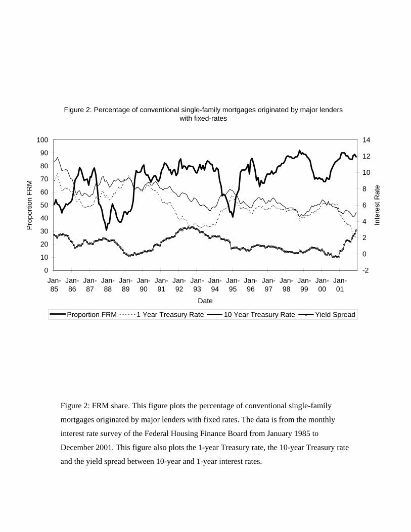
Figure 2: FRM share. This figure plots the percentage of conventional single-family

mortgages originated by major lenders with fixed rates. The data is from the monthly

interest rate survey of the Federal Housing Finance Board from January 1985 to

December 2001. This figure also plots the 1-year Treasury rate, the 10-year Treasury rate

and the yield spread between 10-year and 1-year interest rates.

Figure 2: Percentage of conventional single-family mortgages originated by major lenders with fixed-rates

0

10

20

30

40

50

60

70

80

90

100

Jan-85

Jan-86

Jan-87

Jan-88

Jan-89

Jan-90

Jan-91

Jan-92

Jan-93

Jan-94

Jan-95

Jan-96

Jan-97

Jan-98

Jan-99

Jan-00

Jan-01

Date

Pro

port

ion

FR

M

-2

0

2

4

6

8

10

12

14

Inte

rest

Rat

e

Proportion FRM 1 Year Treasury Rate 10 Year Treasury Rate Yield Spread

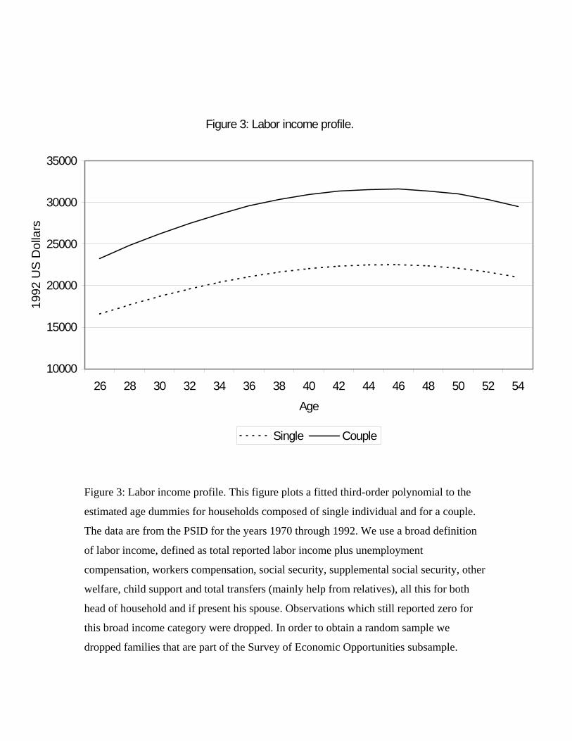
Figure 3: Labor income profile. This figure plots a fitted third-order polynomial to the

estimated age dummies for households composed of single individual and for a couple.

The data are from the PSID for the years 1970 through 1992. We use a broad definition

of labor income, defined as total reported labor income plus unemployment

compensation, workers compensation, social security, supplemental social security, other

welfare, child support and total transfers (mainly help from relatives), all this for both

head of household and if present his spouse. Observations which still reported zero for

this broad income category were dropped. In order to obtain a random sample we

dropped families that are part of the Survey of Economic Opportunities subsample.

Figure 3: Labor income profile.

10000

15000

20000

25000

30000

35000

26 28 30 32 34 36 38 40 42 44 46 48 50 52 54

Age

1992

US

Dol

lars

Single Couple

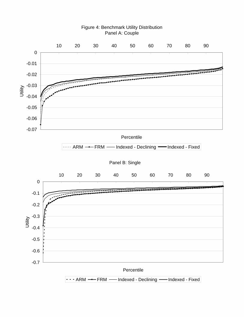
Figure 4: Benchmark Utility DistributionPanel A: Couple

-0.07

-0.06

-0.05

-0.04

-0.03

-0.02

-0.01

0

10 20 30 40 50 60 70 80 90

Percentile

Util

ity

ARM FRM Indexed - Declining Indexed - Fixed

Panel B: Single

-0.7

-0.6

-0.5

-0.4

-0.3

-0.2

-0.1

0

10 20 30 40 50 60 70 80 90

Percentile

Util

ity

ARM FRM Indexed - Declining Indexed - Fixed

Figure 4: Benchmark utility distribution. This figure shows various percentiles of the

distribution of realized utility when we simulate the model for 1,000 households. Panel

shows the results for households composed of a couple and panel B for households

composed of a single individual. The parameters of the model are given in Table 1, with

the size of the house that needs to be financed equal to $187,500. The figure illustrates

utility for an ARM and a nominal FRM with refinancing cost of $1,000, an inflation-

indexed FRM whose real payments which diminish at the average rate of inflation, and

an inflation-indexed FRM with fixed real mortgage payments.

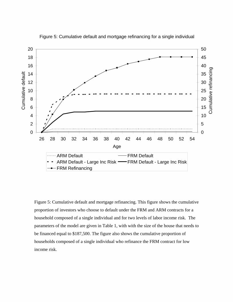
Figure 5: Cumulative default and mortgage refinancing. This figure shows the cumulative

proportion of investors who choose to default under the FRM and ARM contracts for a

household composed of a single individual and for two levels of labor income risk. The

parameters of the model are given in Table 1, with with the size of the house that needs to

be financed equal to $187,500. The figure also shows the cumulative proportion of

households composed of a single individual who refinance the FRM contract for low

income risk.

Figure 5: Cumulative default and mortgage refinancing for a single individual

0

2

4

6

8

10

12

14

16

18

20

26 28 30 32 34 36 38 40 42 44 46 48 50 52 54

Age

Cum

ulat

ive

defa

ult

0

5

10

15

20

25

30

35

40

45

50

Cum

ulat

ive

refin

anci

ng

ARM Default FRM DefaultARM Default - Large Inc Risk FRM Default - Large Inc RiskFRM Refinancing