Home is Where the Equity Is:

Mortgage Refinancing and Household Consumption

Erik Hurst

Graduate School of Business University of Chicago

Chicago, Illinois 60637

and

Frank Stafford Department of Economics

Institute for Social Research University of Michigan

Ann Arbor, Michigan 48109 - 1220

January 2003

We thank members of the Public Finance and Macroeconomics seminars at the University of Michigan and seminar participants at the Federal Reserve Bank of New York, the Inter-American Development Bank, and Indiana University for helpful comments on earlier drafts of this paper. We thank seminar participants at the Federal Reserve Bank of Chicago, the University of Chicago and NBER’s 2001 Summer Institute for Real Estate and Public Policy for comments on this draft. Special thanks go to Axel Anderson, Mark Aguiar, Bob Barsky, Susanto Basu, Paul Bennett, Olivier Blanchard, Dennis Capozza, Kerwin Charles, Paul Courant, Scott Fay, Eric French, Ned Gramlich, Ricardo Hausmann, Michael Hanson, John Laitner, Cara Lown, Jonathan Parker, Matthew Shapiro, Nick Souleles and two anonymous referees. The authors would also like to thank Rob Martin for his excellent research assistance. Support for this research from Citicorp Credit Services and the University of Chicago's Graduate School of Business is gratefully acknowledged. Hurst would also like to thank the financial support given by the William Ladany Faculty Research Fund at the Graduate School of Business, University of Chicago for work on this project. Opinions expressed are those of the authors. Comments may be mailed to erik.hurst@gsb.uchicago.edu.

Journal of Money, Credit and Banking, December 2004

Home is Where the Equity Is:

Mortgage Refinancing and Household Consumption *

Erik Hurst Frank Stafford Assistant Professor of Economics Professor of Economics University of Chicago, GSB University of Michigan

Abstract: Applying a permanent income model with exogenous liquidity constraints and mortgage behavior, household refinancing when mortgage interest rates are historically high and rising, a persistent empirical puzzle, is explained. Using data from the Panel Study of Income Dynamics, households experiencing an unemployment shock and having limited initial liquid assets to draw upon are shown to have been 25% more likely to refinance, 1991-1994. On average, such liquidity constrained households converted over two-thirds of every dollar of equity they removed into current consumption as mortgage rates plummeted, 1991-1994, producing an estimated expenditure stimulus of at least $28 billion. * We thank members of the Public Finance and Macroeconomics seminars at the University of Michigan and seminar participants at the Federal Reserve Bank of New York, the Inter-American Development Bank, and Indiana University for helpful comments on earlier drafts of this paper. We thank seminar participants at the Federal Reserve Bank of Chicago, the University of Chicago and NBER’s 2001 Summer Institute for Real Estate and Public Policy for comments on this draft. Special thanks go to Axel Anderson, Mark Aguiar, Bob Barsky, Susanto Basu, Paul Bennett, Olivier Blanchard, Dennis Capozza, Kerwin Charles, Paul Courant, Scott Fay, Eric French, Ned Gramlich, Ricardo Hausmann, Michael Hanson, John Laitner, Cara Lown, Jonathan Parker, Matthew Shapiro, Nick Souleles and two anonymous referees. The authors would also like to thank Rob Martin for his excellent research assistance. Support for this research from Citicorp Credit Services and the University of Chicago's Graduate School of Business is gratefully acknowledged. Hurst would also like to thank the financial support given by the William Ladany Faculty Research Fund at the Graduate School of Business, University of Chicago for work on this project. Opinions expressed are those of the authors. Comments may be mailed to erik.hurst@gsb.uchicago.edu. .

1

I. INTRODUCTION

The extent to which refinancing activity by homeowners provides a net economic stimulus during

times of falling mortgage interest rates has been a topic of discussion by policy makers during the recent

economic slowdown of 2001-2002. 1 Housing is by far the largest single non-pension asset in a

household’s portfolio, comprising over 35% of the median household's wealth (Hurst, Luoh and Stafford

1998), about two-thirds of families are homeowners. However, unlike drawing down other non-pension

assets, accessing home equity often entails large pecuniary costs. The fixed closing costs alone associated

with refinancing a mortgage or applying for a second mortgage are estimated at 1.5 to 2.5 percent of the

household's initial mortgage balance (Bennett, Peach and Peristiani 1998). Adding in the costs of

searching for a lender, filling out mortgage applications, preparing documentation, paying prepayment

penalties and potentially paying a high marginal borrowing costs on the equity removed can significantly

increase the actual amount that a household has to pay in order to access home equity.

In this paper, we explore the use of home equity as a mechanism by which households smooth their

consumption over time. When confronted with a negative income shock, a household can sustain their

consumption by either drawing down their “more-liquid” assets or, alternatively, tapping into their home

equity. If the household has sufficient amounts of more-liquid assets (checking account balances, stocks,

etc.) it is relatively easy for them to costlessly smooth their consumption. However, it becomes

increasingly difficult for a household to buffer income shocks when these liquid asset balances are low,

especially if non-collateralized borrowing rates are high. Households who have accumulated equity in

their home may choose to pay the fixed cost to refinance and draw down their home equity. But, for a

subset of homeowners, their housing equity is essentially trapped in the home; the gain in lifetime utility

from refinancing and increasing current consumption would not be sufficient to offset the costs incurred

to access the home equity. These households may be appropriately characterized as being liquidity

constrained even though they had equity in their home.2 While there has been much academic work

looking at whether households behave as permanent income consumers (for a survey see Browning and

2

Lusardi 1996), the extent to which households use home equity as a financial buffer has been relatively

overlooked. This omission is surprising given, as noted above, that for most households, the home is

where the equity is.

In the first part of this paper, a model of optimal refinancing incorporating the household's desire to

access home equity is developed. This model highlights two distinct reasons why a household may

choose to refinance: 1) In periods of relatively low interest rates, the household would refinance to

receive a lower stream of mortgage payments and consequently receive an increase in lifetime wealth -

referred to as the “financial motivation”, and 2) households may refinance so as to access accumulated

home equity - referred to as the “consumption smoothing motivation”. Households who received a

negative income shock and who have little liquid assets to buffer the shock are shown to be more likely to

refinance and access home equity, all else equal. This consumption smoothing motivation can explain the

fact that some households will refinance even in a world of stable or rising interest rates, which has been

characterized as an empirical anomaly in the housing literature (Stanton 1995 and Agarwal, Driscoll, and

Laibson 2002).

Using micro data from the Panel Study of Income Dynamics (PSID), strong evidence for our

theoretical predictions is found; the house is used as a mechanism to smooth income shocks and

reductions in the cost of refinancing alleviates otherwise binding liquidity constraints. We regressed

whether a household refinanced anytime between 1991 and 1996 on the household’s permanent income,

demographics, the present value financial gain to refinancing, and controls for the consumption

smoothing motivation to refinance. Households who experienced a spell of unemployment between 1991

and 1996, and who had zero liquid assets going into 1991, were 8 percentage points, or 25%, more likely

to refinance than otherwise similar households. These same households were also more likely to remove

equity during the refinancing process. Furthermore, the propensity to refinance and remove equity for

households who experienced a negative income shock declined as the amount of liquid assets that they

held increased.

3

Using a broader definition of liquidity constraints, we distinguished empirically those who

refinanced primarily to improve their balance sheets from those who refinanced in part to access their

home equity. The latter group exhibits what can be termed as a high average propensity to convert home

equity into current consumption. Households who removed so much equity while refinancing so as to

pay private mortgage insurance converted over 60 cents out of every dollar they removed into current

consumption. Non-liquidity constrained refinancers also removed equity during the refinancing process.

However, these households, on average, did not convert any of the equity they removed into current

consumption - they simply shifted that equity to other portfolio components.

Finally, we discuss how declining mortgage rates can lead to an aggregate net spending stimulus as

otherwise liquidity constrained households are now able to access their home equity at a lower net cost.

We estimate that between 1991-1994, when mortgage rates fell substantially, previously liquidity

constrained households increased aggregate consumption, via refinancing, by a minimum of $28 billion.

II. SUMMARY OF PREVIOUS RESEARCH

There is growing evidence that the home is used as a buffer against adverse shocks. Carroll,

Dynan and Krane (1999) study whether households with a greater risk of unemployment are more likely

to hold assets to buffer the potential shocks. They found a significant precautionary motive in a broad

measure of wealth that included home equity, but found no such precautionary motive in more liquid

forms of wealth. The suggestion that homeowners use their home as a potential buffer is also supported

in Skinner (1996). Households who were early in their lifecycle increased their consumption in response

to an unexpected housing windfall. In contrast households did not alter their consumption in response to

an unexpected housing windfall later in their lifecycle. Such households only responded to a rapid

appreciation in house prices if they experienced adverse economic events. These disparate findings are

reconciled by suggesting that "the home is used as a key component in insuring against retirement

contingencies". Engelhardt (1996) finds similar results.

4

Refinancing activity was on the rise during the early 1990s. Not only was it a period of relatively

low mortgage rates, but it has been argued that mortgage markets were under going structural changes.

Bennett, Peach and Peristiani (1998) have concluded that accessing home equity has become much easier

in the 1990s relative to the 1980s. They find that competition in primary mortgage markets,

improvements in information processing technology, the streamlining of the mortgage application and

approval process and an increase in financially savvy homeowners have led to a dramatic reduction in the

costs associated with accessing home equity. The reduction in these costs appear to have led to more

refinancing during the early 1990s than was predicted by traditional models of prepayment. Brady,

Canner and Maki (2000) report that, in 1994, 45% of mortgage debt holders had refinanced their

mortgage at some time in the past. A majority of these homeowners had refinanced in the 1993-1994

period.

Despite the potential for housing equity to be used as a financial buffer, there is little formal

empirical or theoretical work that explores whether households access home equity so as to smooth

consumption. Much of the work on mortgage refinancing has focused on purely “financial' motivations”

(Curley and Guttentag (1974); Green and Shoven (1986); and Quigley (1987)). When current mortgage

rates are below the existing mortgage contract rate, households have an incentive to replace their existing

fixed rate mortgage with one at a lower rate, thereby reducing their monthly mortgage payments. The

benefit to the household is a present value wealth gain. This benefit only need exceed the time and

money costs of acquiring the new mortgage - which, as discussed above, can be quite large. Chen and

Ling (1989) and Kau and Keehan (1995) extended this approach by developing contingent claims

frameworks embodying a dynamic model of the decision to refinance.

While current and expected future interest rate movements can forecast a great deal of refinancing

behavior, both Stanton (1995) and Agarwal, Driscoll and Laibson (2002) note that these financially

motivated models of refinancing fail to explain some important empirical patterns. Some fixed rate

mortgages are prepaid even when current market mortgage rates are above the household's contracted

5

coupon rate. Such refinancing behavior is often classified as “suboptimal” (Stanton 1995) or

“anomalous” (Agarwal et al 2002). Gilberto and Thibodeau (1989), Dickson and Heuson (1993) and

VanderHoff (1996) suggest that a household may choose to refinance so as to remove equity to invest in

the stock market or to expand their housing stock as family size grows. While these papers illustrate

circumstances in which households would refinance in periods of high interest rates, none of them

formalize a model of the consumption smoothing benefits from accessing home equity, nor do they relate

the refinancing behavior to income shocks or explain differences in behavior between liquidity

constrained and non-liquidity constrained borrowers.

In this paper, we abstract from the lender side of the market. 3 We develop a utility based model

where households optimally choose to refinance even in periods when interest rates are constant or rising.

Such households refinance to access their accumulated home equity so as to smooth their consumption as

their income fluctuates. We refer to the access of home equity as refinancing even though refinancing is

only one means of liquidating the equity.4 The general outline of the theoretical model applies to any

method of accessing home equity, such as home equity lines of credit or to second mortgages, as long as

accessing the home equity imposes some non-trivial fixed cost on the borrower. For the empirical work,

we focus on refinancing because it was the prevalent method of adjusting home equity during the period

we are studying – the early to mid 1990s.

III. THE REFINANCING DECISION IN A PERMANENT INCOME MODEL

This section sets out a model in which households are allowed to use their home equity as a financial

buffer. Each household is endowed with a fixed housing stock. In each period, households optimally

choose consumption, savings, and mortgage borrowing. A key feature to this model is that the agents

face different borrowing and lending rates. Additionally, the agents may not borrow more than their

endowed value of housing stock. Finally, the agents must pay a fixed cost in order to change the total

quantity borrowed. We choose to interpret the borrowing in this model as a secured loan on the housing

stock. We will refer to changes in the borrowing levels as refinancing. For simplicity, households are not

6

allowed to alter their housing stock and the utility generated by consuming the flow of housing services is

ignored.5 The house is treated as an asset in which the household can choose to add or remove savings

after paying a fixed cost. The difference between mortgage interest rates and the interest rate earned on

liquid assets implies the house would be the dominant asset in the absence of transaction costs. Only in

the presence of costs to access home equity will we observe households simultaneously holding both

liquid assets and mortgage debt.

A. The Model

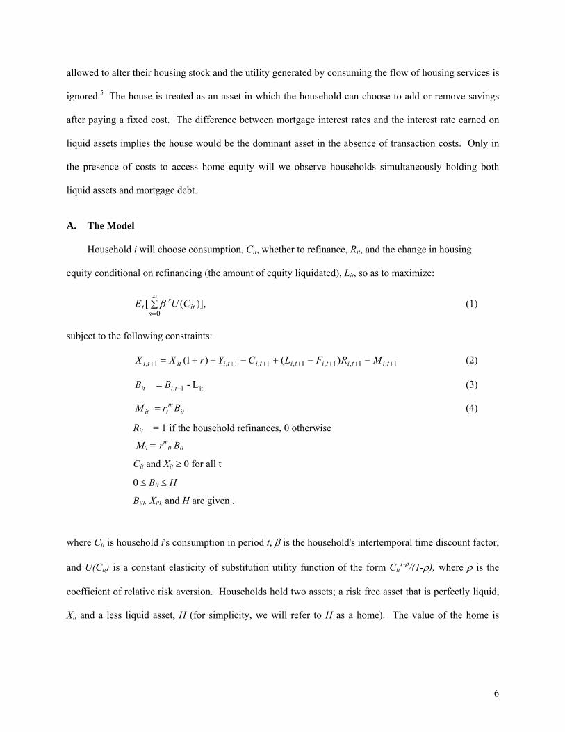
Household i will choose consumption, Cit, whether to refinance, Rit, and the change in housing

equity conditional on refinancing (the amount of equity liquidated), Lit, so as to maximize:

)],([0

sit

st CUE (1)

subject to the following constraints:

1,1,1,1,1,1,1, )()1( titititititiitti MRFLCYrXX (2)

L- it1, tiit BB (3)

itm

tit BrM (4)

Rit = 1 if the household refinances, 0 otherwise

M0 = rm0 B0

Cit and Xit 0 for all t

0 Bit H

Bi0, Xi0, and H are given ,

where Cit is household i's consumption in period t, is the household's intertemporal time discount factor,

and U(Cit) is a constant elasticity of substitution utility function of the form Cit1-/(1-), where is the

coefficient of relative risk aversion. Households hold two assets; a risk free asset that is perfectly liquid,

Xit and a less liquid asset, H (for simplicity, we will refer to H as a home). The value of the home is

7

constant in all periods.6 We explicitly build binding liquidity constraints into our model; households

cannot be a net debtor in either X or H.

Households are endowed with an interest only “mortgage” tied to H in period 0, B0. As a result,

households start with equity in their home equal to (H - B0). If the household has outstanding mortgage

debt (Bit > 0 ), they must make a mortgage payment equal to the interest on the mortgage balance at an

after tax mortgage interest rate of rm0 , the mortgage interest rate. The liquid asset, X, earns an after tax

rate of return equal to r in all periods. We also assume that H, r and rm are exogenous and believed to be

constant over the infinite horizon by all households.

In each period, households choose consumption, whether to refinance, Rit, and the amount of equity

to add or remove from the home, conditional on refinancing. If a household chooses to refinance, the

new mortgage payments are computed the new outstanding mortgage balance multiplied by the

outstanding mortgage interest rates that prevailed in the period in which the household refinanced. The

optimal amount of equity removed from or added to the illiquid asset when the household refinances is

denoted as Lit. If the household refinances in period t, it must pay fixed cost F.

Households face income uncertainty. Household income in period t, Yit, follows a Markov process

with three independent states of the world - low income, medium income and high income:7

Income t

Low Income Medium Income High Income

Low Income .2 .4 .4

Income t-1 Medium Income .2 .4 .4

High Income .2 .4 .4

The low income state corresponds to ‘unemployment’. We set the probability of being unemployed equal

to 0.2, which is about the probability of being unemployed anytime between 1991 and 1996 for

households in our data (see Table 2, discussed below). The probability of being in either the medium or

8

the high income states is 0.4. We set the low income value to 0.3 and the median income value equal to

0.6. The 0.3 corresponds to the median ratio of labor income plus transfers relative to house value for

unemployed households in our sample. This 0.6 corresponds to the median ratio of labor income plus

transfers relative to house value for all employed households in our sample. We set the high income

value equal to the value of the housing stock, 1. Finally, we set the return on the risk free liquid asset to

0.03, the mortgage rate to 0.065, the time discount factor to 0.85, and the fixed cost to refinancing to be

2% of the house value.8

The timing of the household’s decision in period t is as follows: 1) The household enters the period

with outstanding mortgage balance (Bt-1) and an existing stock of liquid assets (Xt-1). 2) The household

receives an income realization in the current period (Yt). 3) The household decides whether to refinance

(Rt) and the amount of equity to remove (Lt). This decision determines the mortgage balance to be carried

into the following period (Bt). 4) Lastly, the household chooses consumption today (Ct) and the savings

to be carried over to next period (Xt). It should be noted that the purpose of the theoretical exploration is

to identify important dimensions of the consumer optimization problem and the refinancing decision

when the household has the choice to access housing equity, but at a cost. These qualitative results

provide guidelines for the empirical work that follows.

Using numerical solution techniques, there are several interesting results that come from our

theoretical example. Figure 1 shows household refinancing behavior in a world with no interest rate

movements as a function of the liquid assets held by the household at the beginning of the period (Xt-1),

the outstanding mortgage balance of the household at the beginning of the period (Bt-1) and the current

income realization of the household (Yt). Figure 1 has three panels labeled a, b and c, corresponding to

the three income realizations (low, medium and high). The shaded area in each of the panels indicates

which households will refinance in the current period as a function of Bt-1 and Xt-1, for each Yt realization.

Comparing across panels, it is seen that households with low income realizations are much more likely to

refinance than households who receive medium or high income draws. In fact, a household who receives

9

a high income realization does not refinance at all under this parameterization. Panel a) further illustrates

that not all households who receive low income realizations will refinance; only those households with

equity in their home and with little initial liquid assets to buffer the shock. Our model generates what has

previously been described as an empirical anomaly; utility maximizing households will optimally choose

to refinance in a world with stable interest rates.

These results are quite intuitively appealing. If a household received a high income realization and

that household had low liquid wealth, there is no need for them to tap into their home equity to sustain

their consumption. To the contrary, such a household would likely save a portion of their income

realization (in liquid assets) so as to fund consumption in future periods. Additionally, households with

high beginning of period liquid assets who receive a low income shock do not refinance. Such a

household could buffer the low income realization using their liquid assets, which they can access without

cost. It is the combination of low initial liquid assets and a low income realization that predicts

refinancing. Figure 1 generates the first prediction which we will test empirically: households who

receive a low income realization (relative to their expected permanent income), who have low liquid

assets, and who have equity in their home will be willing to pay the associated costs to refinance.

Although the results are not shown, the households refinancing in figure 1 removed substantial

amounts of equity when refinancing. This is not surprising given that the household is refinancing to

access the home equity. Lastly, it can be easily shown that the equity removed was used to fund current

consumption. In other words, if the household did not to refinance (i.e., the cost of refinancing was

prohibitively large), their consumption would be much less than their post-refinancing consumption.

Two further comments about our model are noteworthy. First, it is worth discussing the implication

of different income ‘shocks’. The income process we specified in our numerical example has both

permanent and transitory components. However, if the income process was either a pure random walk or

pure i.i.d. with a constant mean, the results would be intuitively the same. The decision rule of the

household is to compare the benefits of refinancing (in terms of the increase in lifetime utility from

10

smoothing consumption) to the costs of refinancing (the loss in utility associated with paying the

refinancing fees). In our empirical work below, we will focus on unemployment shocks. While

unemployment shocks have both a permanent and a transitory component, they are thought to be much

more temporary than permanent (Huff-Stevens 1997). Given that permanent shocks would be likely to

induce many households to alter their housing stock, empirically focusing on large transitory shocks is

more in the spirit of our model. For completeness, we do account for the possibility of moving in our

some of our empirical specifications.

Second, our model adds to the existing literature by isolating two separate motives to refinance. The

models of financially motivated refinancing studied by other authors conclude that households only

refinance when current mortgage rates are lower than the mortgage rate on the existing mortgage contract.

As interest rates fall, households will refinance if the present value gain in wealth from reducing

mortgage payments exceeds the cost of refinancing. However, as shown above, households will also

refinance to tap into their home equity. These two motives to refinance are not independent. For

households who have low initial liquid assets and who received a low income realization, the refinancing

rule when interest rates fall differs from the rule followed by other households. These households who

received a negative income shock and who have low liquid wealth will refinance when the lifetime utility

gain from lower mortgage payments plus the lifetime utility gain from accessing home equity exceed the

utility loss from paying the refinancing costs. All else equal, these households will be induced to

refinance at smaller interest rate differentials.

Given this, our model shows that there is a role for monetary policy in alleviating liquidity

constraints faced by homeowners with equity remaining in their home. By lowering interest rates, the

Fed reduces the effective cost of accessing home equity. Prior to the declining interest rates, homeowners

would only receive a consumption smoothing benefit if they choose to refinance. If this benefit is smaller

than the utility loss from paying the refinancing costs, such households would not refinance. In essence,

their housing equity would be trapped. But, if mortgage rates fall, the household would have two benefits

11

to refinance; the financial benefit and the consumption smoothing benefit. Such households would be

more likely to refinance and access their pent-up home equity (because the benefits increased).

Reducing mortgage rates could stimulate refinancing, allowing otherwise liquidity constrained

households with equity trapped in their home to access that equity and fund current consumption.

Before we get to our empirical work, we show that our simple theory is consistent with the aggregate

time series of refinancing behavior. Table 1 summarizes data compiled by Freddie Mac Corporation.

Column 1 of Table 1 lists the average annual 30-year fixed mortgage rate between 1986 and 1998,

Column 2 presents the share of all mortgage originations that were refinancing, while Columns 3 and 4,

respectively, show the percentage of refinancers who removed equity from their home and the percentage

of refinancers who added equity to their home. During the late 1980s, when mortgage rates were high,

the overall refinancing share was low, but those who did refinance were very likely to ‘refinance up’,

increasing overall mortgage debt as part of the refinance process. In terms of the theory, those who

refinanced in periods of relatively high interest rates were more likely to remove housing equity; this is

consistent with these refinancing households being motivated by consumption smoothing.

As mortgage rates fell in 1993 and 1994, the overall refinancing rate rose strongly, but the share of

those removing equity fell, meaning that most refinancers were motivated solely by wealth gains. Note

that in 1993, 20 percent of refinancers added equity (‘refinanced down’) during the refinancing process.

This is not unexpected, and consistent with the theory above, given that many households are likely to

reallocate their portfolio between housing equity and other assets as they refinance.

Recent work by Brady, Canner and Maki (2000) is also consistent with the model of refinancing

discussed above. These authors summarized the March through May 1999 University of Michigan's

Surveys of Consumers' questions asking households if they refinanced, whether they removed equity

when they refinanced and what they did with the equity that they removed. They found that about 35%

of households removed equity while refinancing during the low mortgage rate period of 1998. Of those

who removed equity, 43% took out less than $10,000 and 26% took out more than $25,000. The mean

12

amount liquefied was more than $18,000 and the median amount was over $10,000. Of the total amount

of equity removed during the refinancing process, 20% of that amount was used for current consumption

while the remaining 80% was shifted to other portfolio components including a portion which was

reinvested back into the home via home improvements.9 This is predicted by our theory. In periods of

low mortgage rates, households will refinance to lock in lower interest rates. Many of these households

will remove equity. Some will simply use these funds to reallocate their portfolio. But others will use the

opportunity of low interest rates to access home equity, which was otherwise trapped in their home when

interest rates were high, so as to fund current consumption.

IV. Data

Observations from the Panel Study of Income Dynamics (PSID), a large-scale longitudinal study of

U.S. households starting in 1968, were used for the research. Since 1980, the PSID has tracked housing

decisions by asking detailed mortgage questions. In each year of the survey, households are asked to

report their own estimated value of their house and, if applicable, to report the terms of their mortgage

(mortgage balance, monthly payment net of taxes and insurance, and the years remaining on the loan). In

1996, a special supplement to the PSID core survey focused on mortgage shopping. In this supplement,

households were asked whether they refinanced their mortgage during the 1990s and if so, in what years.

Additionally, households were asked to provide the rate they are paying on their current mortgage and the

effort they put forth in searching for their current mortgage lender. The core PSID survey asks detailed

questions on the respondent’s earnings, family structure and demographics. The PSID Wealth

Supplements, in 1984, 1989 and 1994, asked respondents questions about their current financial

position.10

Our sample included all households in the PSID owning their main home continuously between

1989 and 1996, who had a mortgage, who did not move any time during the period and who had positive

average labor income between 1991 and 1996. In total, the sample included 1,606 households. Some

observations with obvious data entry errors or missing values were dropped, reducing the sample size to

13

1,448 households. Of the 1,448 households, 434 refinanced between 1991 and 1996. Corresponding to

aggregate data, approximately 31% of mortgage holders in our sample (weighted average, using PSID

weights) refinanced during the early 1990s with the majority of refinancing taking place between 1993

and 1994 - again, matching the aggregate time series data.

V. Consumption Smoothing and Household Refinancing Probabilities

In this section, using our sample of PSID homeowners discussed above, we empirically test one of

the key results from our theoretical model. If households use their home equity to smooth consumption,

we would predict that those who received both a negative income shock and who had low levels of pre-

existing liquid assets would be more likely to refinance, all else equal. This would be especially true in

periods of lower mortgage rates, such as the early 1990s, where the net-cost of accessing home equity was

reduced.

Three caveats are of note when trying to test our theory empirically. First, as discussed above, not

all households who receive a negative income shock will refinance to access home equity, only those

households who do not have other lower cost options to smooth the shock. A series of successive bad

shocks could cause historically high saving households to be left with little liquid assets, forcing them to

tap into their home equity to smooth additional shocks. Second, also discussed above, both permanent

and transitory income shocks could cause households with little liquid assets to refinance. The

household will refinance any time the gain in lifetime utility from increasing consumption is greater than

the cost of refinancing. The benefits of refinancing increase if a given size shock in the current period is

permanent, but in such cases, it is likely that the household would also want to change the size of their

housing stock. Given that we restrict our sample to non-moving households, our empirical work will

focus on the impact of unemployment shocks which are more temporary in nature.

Third, households will respond to both expected and unexpected shocks, particularly in periods of

low interest rates. Suppose in 1990 a household with very little liquid assets, but a large amount of

housing equity, knew for certain that she would become unemployed in 1993. Given the relatively high

14

interest rates in 1990, 1991 and 1992, a perfect foresight household would wait until 1993 before

refinancing. The refinancing would take place in the year of the income shock, even though the shock

was perfectly anticipated. Conversely, if the household head in 1993 found out that she would lose her

job in 1994, a perfect foresight household would respond to the predictable shock in the low interest

period of 1993. In this case, the refinancing would occur prior to the arrival of the income shock. Such

timing issues need to be accounted for empirically. Unemployment spells in 1994, if predicted, could

have resulted in refinancing in 1993. Below, we discuss how we address each of these caveats

empirically.

To test the proposition that households use their home to buffer income shocks, we run a cross

section regression predicting whether the household refinanced any time between 1991 and 1996 as a

function of the financial gain from locking in lower interest rates during this period, demographics and

controls for the consumption smoothing benefits to refinance. The reduced form refinancing decision for

households over this period can be formalized as:

Yi = 0 + 1 PVWealth,i + 2 ConSmoothi + 3 Demi + β4 Incomei + i; (5)

where Yi becomes the unobservable gain from refinancing, PVWealth,i , defined below, is the present value

wealth gain of locking in lower mortgage rates, ConSmoothi represents a vector of variables reflecting the

household’s desire to access interim home equity, Demi and Incomei are vectors of demographic and

income controls, respectively, that could affect the refinancing decision, and i is a normally distributed

white noise error term. The observed variable is Refii, which equals one if household i refinanced

between 1991 and 1996, and zero otherwise. We estimated the probability that Refii = 1 using standard

probit techniques.

Because the household only reported refinancing behavior retrospectively in 1996 and is only asked

about their most recent refinancing experience (back through 1991), we cannot take advantage of the

panel aspect of our data. As a result, all our regressions are cross sectional regressions predicting

refinancing behavior anytime between 1991 and 1996. Averaging over the years will also likely mitigate

15

measurement error in all the variables we used in our regression. More importantly, treating our data as a

cross section allows us to better address the timing of predictable and unpredictable shocks, discussed

above. If households have perfect foresight, they may wait until the period of low interest rates to

respond to past or expected future shocks. To address these timing concerns, we test whether income

shocks received anytime between 1991 and 1996 affect refinancing anytime between 1991 and 1996.

For robustness, we estimated a stacked regression predicting refinancing in year t, as a function of only

year t-1 characteristics, where t equals all years between 1991 and 1996. The results (not reported) were

quantitatively similar in point estimates to the results we report below, although, as expected given the

potential measurement error and the neglect in dealing with timing issues, the standard errors were

slightly larger.

Consistent with the existing literature, we constructed a measure of the present value wealth gain

(the value of the financial option) that households would receive if they refinanced during the 1993-1994

period and locked in the low interest rates that prevailed during those years. The present value of pure

wealth gains from an interest rate change can be expressed as the difference between households’

mortgage payments under the new rate and the mortgage payments under their original mortgage rate,

discounted over the remaining length under the old mortgage.11 Assuming that the mortgage balance or

the term of the mortgage is not altered during the refinancing process, we can represent the present value

wealth gain from refinancing in continuous time as:

PVWealth,it = Max [Bit 00( ) /(1 )

iT si it itr ds , 0]; where (6)

i0 = )e(1

r

iTmi0r

mi0

and it = )e(1

r

iTmitr

mit

,

and where PVWealth,it is the present value of wealth gains for household i refinancing in year t truncated at

zero, Ti represents the number of periods remaining on household i’s original mortgage, rit is the rate at

which the household discounts future income (assumed to be 3 percent), rmi0 is the original mortgage rate

16

(after tax) on household i’s mortgage, rmit is the after tax mortgage rate had the household refinanced in

October of 1993, and Bit is the outstanding balance on household i’s mortgage in year t.12 The higher

PVWealth,it for the household, the greater the likelihood that the household will refinance in a given period.

Almost all studies of refinancing use this measure (potentially adjusted for future interest rate

movements) as the sole measure of demand for refinancing.

We use unemployment spells as our measure of income shocks. In relation to our theory,

unemployment spells tend to be more temporary than permanent. Formally, the variable Unempi is a

dummy variable taking the value of 1 if either the household head or the spouse experienced an

unemployment spell between 1991 and 1996. Just as almost all of the households in our sample who

refinanced did so between 1993 and 1994, almost all of the unemployment spells in our sample occurred

prior to the end of 1993. This is not surprising given the macroeconomic conditions that prevailed in the

United States prior to and after 1993.

As seen in Section III, unemployment, per se, does not predict refinancing for consumption

smoothing reasons. If a household has sufficient liquid assets, it can buffer the income shock by drawing

down these assets. However, households who have little liquid assets prior to the receipt of the shock will

have to pay the fixed costs of refinancing so as to access their accumulated home equity. To test the

theory, the unemployment shock was interacted with the liquid assets that the household had in 1989 (the

last time liquid assets were measured in the PSID prior to our sample period).13 Additionally, we include

a triple interaction between the unemployment shock, the liquid assets, and the amount of equity the

household had in their home in 1990 (the period directly prior to the start of our sample period). We

measure home equity by the household’s loan to value ratio (LTV), defined as the households remaining

mortgage balance in year t relative to their self reported house value in year t. The regressions also

separately include controls for the household’s LTV in 1990 and the value of liquid assets in 1989. Given

that lenders require households with a LTV above 0.8 to purchase costly private mortgage insurance and

may exclude borrowers completely with a LTV above 0.9, we also include a dummy variable for whether

17

the household had a LTV in 1990 between 0.8 and 0.9 and a dummy variable for whether they had a LTV

in 1990 above 0.9.

We predict the sign on Unempi to be positive, the sign on the unemployment/liquid-asset interaction

to be negative, and the sign on the unemployment/liquid-asset/loan-to-value-ratio triple interaction to be

negative. Households will be more likely to want to tap into their home equity when they receive a

negative income shock, but their desire will diminish as the amount of liquid assets they have increases or

the amount of equity they have in their home falls. Why would a household pay the cost to refinance to

access home equity to smooth their income shock when they have sufficient assets in their checking

account to do so?

To control for additional factors that affect the decision to refinance, we include the following series

of demographics: the change in house value between 1990 and 1995, marital status in 1990, the change

in marital status between 1990 and 1995, the number of children in 1990, the change in the number of

children between 1990 and 1995, a permanent income measure (average household labor income between

1990 and 1995), the age of the household head, a series of education dummies measuring the educational

attainment of the household head, the race of the household head, a series of region dummies for where

the household lived in 1990, and whether the household experienced any financial distress between 1991

and 1996. The means of relevant variables used in our empirical work for those households who

refinanced and those households who did not refinance are shown in Table 2. All dollar amounts reported

in this paper are in 1996 dollars. Refinancers tended to be younger, more educated, more likely to be

married, have higher incomes, and have a higher financial gain from refinancing than other non-

refinancing homeowners.

Columns I-IV of Table 3 presents the results of our estimation of equation (10), where each of the

columns includes different controls for the consumption smoothing motivation to refinance. For space,

we suppressed the coefficients on all the income and demographic controls. Column I reports the results

of a probit regression predicting refinancing as a function of the present value gain to refinancing, all the

18

income and demographic controls and none of the consumption smoothing controls. As anticipated,

households with a higher present value wealth gain from refinancing and locking in the lower mortgage

interest rate were more likely to refinance (p-value < 0.01). This is consistent with much of the existing

literature on the financial motivations to refinance. The marginal effect (reported in column I) is large.

For every $1,000 increase in the present value wealth gain the probability that a household refinances is

predicted to increase by 4.6 percentage points, or 14.4% (0.046/0.32, where 0.32 is the base probability of

refinancing for our sample).

Column II reports the results of a probit regression predicting refinancing that includes all the

controls from regression I, plus some controls for the household’s desire to refinance so as to smooth

consumption. The first thing to note is that the coefficient on the present value wealth gain fell. This is

not surprising. The regression in column II includes controls for the household’s LTV. Households with

a higher LTV, have lower outstanding mortgage debt and as a result, have less of a benefit from locking

in the lower mortgage interest rate. By controlling for the household’s LTV, we are partially controlling

for their present value wealth gain. As is shown in Table 3, refinancing is an increasing function in LTV.

However, households with an LTV above 0.8 are much less likely to refinance than other households.

Lenders will require such households to secure private mortgage insurance, reducing their financial

option to refinance. Additionally, there is little equity to remove from their home, thereby reducing their

consumption smoothing option to refinance.

The results in column (II) provide little direct support for the consumption smoothing hypothesis.

Neither the unemployment measure, nor the liquid asset measure, is statistically significant, although each

entered with the expected sign. But, given this specification, these results are not surprising. Our model

did not predict that all unemployed households will be more likely to refinance, only the unemployed

households with low levels of more-liquid assets. In column (III) of Table 3, we also include an

unemployed/liquid-asset interaction. Here, the results become much stronger. Households who

experienced an unemployment spell in the early 1990s with no liquid assets in 1989 were 8.0 percentage

19

points, or 25% (0.08 divided by the base probability of refinancing for the sample, 0.32), more likely to

refinance their home during the 1991-1996 period (p-value = 0.05). For each additional $10,000 in liquid

assets that the household had in 1989, the probability of refinancing decreased by 1 percentage point or

3.2% (p-value = 0.10). Including the interaction term matches the empirical results with the theoretical

predictions. It is not all households who received a negative income shock that were more likely to

refinance, just those who had little assets to buffer the shock. It should be noted that even in this

specification liquid assets are not statistically significant, only the liquid assets interacted with the

unemployment shock.

The theoretical results above also predict that not all households who had low liquid assets and who

experienced a consumption shock would refinance, only those households who had sufficient home

equity to do so. In regression (IV) of Table 3, we also included a triple interaction of whether the

household experienced an unemployment shock, their initial LTV in 1990 and their liquid assets in 1989.

This interaction came in with the expected sign, although it was not statistically significant. The

unemployment variable by itself increased from 0.08 to 0.16 and it still remained statistically different

from zero (p-value = 0.08).14

As predicted by our theory of the consumption motivation to refinance, these households who

experienced unemployment spells and who had low levels of liquid assets were also more likely to

remove equity during the refinancing process. Table 4 shows the results of a regression predicting the

fraction of equity removed relative to the initial mortgage balance as a function of demographics, income,

unemployment spells and unemployment spells interacted with liquid assets. The demographic and

income controls used in this regression were the same as used in the regressions reported in Table 3.

Because the amount of equity, relative to the initial mortgage balance, that a household would have

removed is not observed for those households who did not refinance, OLS estimation would produce

biased coefficient if there is a correlation between the choice to refinance and the dependent variable in

the regression of Table 4. To address this problem, we ran the Heckman selection procedure with the

20

decision to refinance modeled as in Table 3. We were able to get identification from the fact that the

present value gain from refinancing effects the refinancing decision, but is independent of the fraction of

equity that the household would want to remove during refinancing scaled by the initial mortgage

balance. The identification is driven by the fact that the present value wealth gain is a function of the year

when the initial mortgage was originated. It is not unreasonable to assume that the year in which the

initial mortgage was originated is independent of the desire to remove equity from the home conditional

on refinancing during the mid-1990s. 15 The estimated correlation between the error terms of the

refinancing and equity removed equations was large, but not statistically different from zero ( = 0.67, p-

value 0.46). Although we cannot reject that the error terms between the equity removal equation and the

selection equation were correlated, we still report the results from the Heckman selection model. We

suppressed the first stage results for the probability of refinancing when reporting the results of the

Heckman selection model in Table 4. It should be noted that the results reported in Table 4 were nearly

identical to the results from the OLS estimation.

The average amount of equity removed for the sample was 9% of their initial mortgage balance. As

predicted, households who experienced an unemployment spell and had zero liquid assets in 1989

removed 12 percentage points more equity, relative to their initial mortgage balance, than other

comparable households when refinancing (p-value = 0.09). As the amount of liquid assets held by the

refinancing households who received an unemployment shock increased, the amount of equity they

removed diminished rapidly.

The predictions of the consumption smoothing theory of refinancing are borne out in the data:

controlling for the present value wealth gain to refinancing and demographics, households who

experienced an unemployment shock, who had low levels of liquid assets and who had equity in their

home both were more likely to refinance and were more likely to remove equity from their home during

the process of refinancing. Was the equity removed used to fund current consumption? We address this

question in the next section.

21

VI. Mortgage Refinancing, Liquidity Constraints and Consumption

It is quite conceivable that forward looking households would have equity trapped in their home. A

series of negative income shocks could easily have depleted a household’s liquid saving. Given the large

fixed costs associated with accessing their home equity, some households may prefer to alter their

consumption away from their optimal path instead of refinancing. We saw such behavior predicted from

the model in Section III. In these instances, households will be essentially liquidity constrained; they

wish to increase their consumption, but are confronted by an unfavorable cost structure. However, the

liquidity constraint can be partially alleviated in periods of declining interest rates as the net benefits to

accessing the accumulated home equity are now larger.

In order to compare the consumption behavior of liquidity constrained refinancing households, we

first have to isolate households who we plausibly believe would be liquidity constrained. In this section,

we are going to analyze a broader group of potentially liquidity constrained refinancers than we did in the

previous section when we focused on households who became unemployed and who had low levels of

liquid assets to buffer the shock. A household could be liquidity constrained for reasons other than

having received a negative income shock. For example, a household could have received positive news

about their income growth prospects, they could have experienced a negative consumption or health

shock, or, simply, they could have a high intertemporal time discount rate.

Existing mortgage regulations allow households who are potentially liquidity constrained, for

whatever reason, to reveal themselves. In order for conventional mortgages to be sold on the secondary

market, all mortgages with an originating loan to value ratio greater than 0.8 must secure private

mortgage insurance. Thus, conventional mortgages have a kink in the mortgage borrowing schedule at a

0.8 loan to value ratio. The effective borrowing rate on the equity removed for households who

refinanced with an initial LTV just below 0.80 to an ex-post refinancing LTV of just above 0.80 can

easily exceed twenty percent (see Caplin et al 1997). The reason for this is that the higher borrowing rate

22

resulting from the private mortgage insurance is applied to the whole outstanding mortgage balance, not

just the incremental equity removed. We posit that households who had a pre-refinancing LTV below

0.8 and who subsequently had a post refinancing LTV above 0.80 were otherwise liquidity constrained.16

For the following empirical work, these households need not be liquidity constrained - we will

empirically test for differences in behavior. But by sub-setting the sample in this way, we are just arguing

that this group, ex ante, by not buying down their mortgage to a 0.8 loan to value ratio, is a likely

candidate for being liquidity constrained.

This section sets out to verify empirically two points: 1) households who crossed the 0.8 LTV

threshold while in the process of refinancing have behavior consistent with being liquidity constrained -

they paid a premium to access home equity, they held low levels of liquid wealth, and they removed large

amounts of equity while refinancing and 2) that these liquidity constrained refinancing households used

the equity they removed while to fund current consumption (while those who had ex-post refinancing

LTVs below 0.8 and who removed equity did not convert the equity into current consumption).

Did the households we designated as being potentially liquidity constrained pay higher rates in order

to refinance? We estimated the loan supply curve offered by lending institutions. Table 5 reports the

results of a regression of the mortgage rates paid by households who refinanced between 1991 and 1996

as a function of household income and demographics, characteristics of the loan and controls for the

default risk of the refinancing household, estimated using a Heckman selection model.17 Demographic

controls used to estimate the loan supply curve include the household head’s 1990 age, marital status in

1990, level of educational attainment, race, average five year labor income between 1991 and 1995 and

household family composition in 1990. The characteristics of the loan include whether the 1996 interest

rate is fixed or variable, whether the loan in 1996 was guaranteed by the Veterans Administration,

whether the loan was insured by the Federal Housing Administration, the term of the mortgage in 1996

and the year the mortgage was originated. The coefficients on all the other additional variables, except

the year the mortgage was originated, were suppressed. The time dummies portray a pattern consistent

23

with Table 1. Interest rates in 1993, 1994 and 1996 were lower than in 1992 and 1995. All the rates were

lower than they were in 1991.

Of note in Table 5 are the controls for the default risk of the household. Not surprising, riskier

borrowers paid higher interest rates. If the household was unemployed in the year that they refinanced,

they paid, on average, 40 basis points higher. Households who reported experiencing some financial

distress during the period (had trouble paying bills, had creditors call to demand payments, were late on

payments) were also more likely to pay a higher interest rate. In this section of the paper, we designated

households who are likely liquidity constrained as those households who had a pre-refinancing loan to

value ratio below 0.8 and then had a post-refinancing loan to value ratio above 0.8. As evidenced in

Table 5, such households, in fact, paid a higher mortgage rate in order to refinance. Those households

with post refinancing loan-to-value ratios between 0.8 and 0.9 had to pay an additional 22 basis points on

average (p-value 0.09) while those above 0.9 had to pay an additional 48 basis points on average (p-value

0.02). These numbers are similar to industry standards where households with loan to value ratios

between 0.8 and 0.9 are required to secure private mortgage insurance which usually costs an additional

quarter of a basis point.

Households that are liquidity constrained likely would have lower levels of liquid assets than other

comparable households. Table 6 shows the means of demographic, income and wealth variables for

homeowners with mortgages who refinanced and removed equity so as to have an ex-post loan to value

ratio greater than 0.8 and homeowners with mortgages who refinanced and had an ex-post loan to value

ratio less than 0.8. One of the major differences between the two refinancing groups was that those who

ended up with a loan to value ratio of 0.8 were, on average, 4 years younger. Given the way the sample is

subsetted, this should not be surprising. Only the households who removed substantial equity so as to

trigger the rate premium when they refinanced were included in this refinancing group. It is possible that

some refinancers removed substantial equity for current consumption without triggering the penalty

24

associated with crossing the 0.8 ex-post loan-to-value ratio threshold. These omitted households would

tend to be older, having had the opportunity to pay down their mortgage over time.

Liquidity constrained refinancers tended to be different from other refinancers (and homeowners in

general) along many other dimensions. The identified liquidity constrained group of refinancers had less

mean and median net worth in 1989 ($101,600 and $41,900, respectively, for the liquidity constrained

group and $171,300 and $106,300, respectively, for the other refinancers). Not only did the identified

liquidity constrained refinancers have lower current total wealth, they also had lower liquid wealth in

1989. The median liquid wealth was $6,200 for the liquidity constrained group and $12,000 for the other

refinancers (p-value of the difference 0.08). The difference persisted at both the mean and the 75th

percentile. The liquidity constrained refinancers were also much more likely to remove equity during

refinancing. 92% of liquidity constrained household removed equity while refinance versus only 57% for

the other refinancers. The average equity removed, conditional on refinancing, was over two and a half

times greater for liquidity constrained households ($43,400 vs $17,200).

We are relatively confident that we isolated a group of households which were liquidity constrained

before they refinanced. This group was willing to pay a large premium to access home equity, they

persistently held lower levels of total and liquid wealth and were more likely to remove large amounts of

equity during refinancing. All of these characteristics are consistent with this group being potentially

liquidity constrained.

The question to which we now turn is whether this liquidity constrained group did, in fact, use the

equity they removed to increase their current consumption. As interest rates fell in the early 1990s, it

reduced the cost of accessing home equity for liquidity constrained households. In the PSID, aside from

food consumption, there are no direct measures of consumption. However, one can back out consumption

changes for PSID homeowners using the detailed wealth and income measures. Conditional on income, if

household saving falls, household consumption must have increased. To test if there are differential

consumption responses between liquidity constrained refinancers who removed equity and non-liquidity

25

constrained refinancers who removed equity, we estimated the following cross sectional equation on a

sample of PSID homeowners:18

ΔWealth89,94 = α0 + α1 Dem89 + α2 ΔDem89,94 + α3 Income89-94 + α4 ΔIncome89,94 + α5 Wealth89

+ α6 Refi91-94 + α7 Refi91-94 * LiqCon + γ1 Refi91-94 * LiqCon * ΔEquity

+ γ2 Refi91-94 * NonLiqCon * ΔEquity + η (7)

where each variable is index by household i, although the i subscripts are suppressed. ΔWealth89,94 is the

change in household i’s total measured wealth, including housing, between 1989 and 1994, Dem89 is a

vector of demographics of household i in year 1989, and ΔDem89,94 is the change in demographic variables

between 1989 and 1994. The demographic variables included are the household head’s age, education,

race, marital status, number of children, census region and sex. The change in demographic variables

included whether the head became married, whether the head became divorced and the change in the

number of children living in the home. Income89-94 is a vector of income controls including household i’s

average family labor income between 1989 and 1994 and the square of this measure. ΔIncome89,94 is the

change in household i’s family labor income between 1989 and 1994. Wealth89 is a vector of initial

wealth controls for household i including the household’s initial 1989 wealth if it was positive, a separate

variable for the household’s 1989 wealth if it was negative, whether the household had any non-

collateralized debt in 1989 and whether the household owned any stocks in 1989. The inclusion of these

variables is designed to capture differences in returns faced by different homeowners. Refi91-94 is a

dummy variable taking the value of 1 if the household refinanced between 1991 and 1994. All

refinancers can be classified as being either liquidity constrained (LiqCon = 1) or non-liquidity

constrained (NonLiqCon = 1). Our identification of who is liquidity constrained is the same as above; a

refinancing household is designated as being liquidity constrained if they refinanced from a LTV less than

0.8 to a LTV above 0.8.

26

As we saw in Table 6, both liquidity constrained and non-liquidity constrained refinancers removed

equity while refinancing. From our theory, we expect the liquidity constrained refinancers to use the

equity they removed to fund current consumption. We would not necessarily expect to observe this

behavior for households who refinanced solely to exercise the financial option. 19 To test these

predictions, we separately included controls for the amount of equity removed (ΔEquity) for both liquidity

constrained refinancers and non-liquidity constrained refinancers. The coefficients on these variables, γ1

and γ2, provide an estimate of the average propensity to convert housing equity into consumption

expenditures (APCE) for both liquidity constrained and non-liquidity constrained households,

respectively. Households who removed equity from their home while refinancing between 1991 and

1994 could either spend it or reallocate that equity to another portfolio component. If the household

spends it, it would no longer show up in any measure of their wealth. However, reallocating the wealth to

another portfolio component would leave total wealth unchanged. We predict that the APCE for

liquidity constrained refinancers (γ1) will be close to negative 1 and the APCE for non-liquidity

constrained refinancers will be zero (γ2). The interpretation is that liquidity constrained refinancers will

spend the equity they remove on current consumption and hence, that equity will disappear from their

portfolio causing their total wealth to fall. The non-liquidity constrained refinancers will remove equity

and use this equity to rebalance their portfolio. Their total wealth, as a result, will not fall when equity is

removed during refinancing.

Table 7 presents the results of estimating (11) via OLS (Row 1) and via a quantile regression at the

median regression (Row 2). We only present the estimates of γ1 (Column I), γ2 (Column II) and the p-

value from a Wald test that γ1 ≤ γ2 (Column III) in this table. The OLS and median regressions estimate

γ1 to be -0.66 and -0.67, respectively (p-values = 0.02 and < 0.01). In other words, for every $1 of equity

removed by the liquidity-constrained household, consumption increased (wealth declined) during that

time period by two-thirds of a dollar. The results are dramatically different for the non-liquidity

constrained households where the APCE is estimated to be 0.20 (OLS) and -0.03 (median), with p-values,

27

respectively, equaling 0.65 and 0.84). We can reject that γ1 ≤ γ2 for both the OLS and median

regressions (p-value = 0.05 and < 0.01, one tailed test, respectively). The data conclude that liquidity

constrained refinancers spend much more of the equity they remove on current consumption. It should

be noted that the OLS estimate of γ1 for liquidity constrained households is not statistically different from

-1, although we can reject that the estimate from the median regression is equal to 1. The fact that the

household did not spend all of the removed equity could be an issue of time. The households primarily

refinanced during 1993 and 1994 and the latest wealth measure was observed in early 1994. It is

possible that households who refinanced and removed equity simply did not have a chance to spend it by

the time their wealth was measured. Given this, our estimates of the APCE for liquidity constrained

households are likely biased towards zero.

The fact that a fall in interest rates can alleviate liquidity constraints by allowing households to

access their home equity at a lower cost has implications for aggregate spending. When the mortgage

rates fell during the early 1990s, liquidity constrained households suddenly were able to access their

trapped home equity at a lower cost. Using the results from Table 7, we can predict the total net

spending stimulus that resulted to the economy when mortgage rates fell during the early 1990s.

Although only a small percentage of the sample is termed liquidity constrained by our definition, these

households removed large amounts of equity when refinancing. 14% of refinancing households increased

their loan to value ratio above 0.8 when refinancing, borrowing an additional $16,000, at the median,

during the process. Using aggregate statistics on the number of households and the number of

homeowners in 1993, and using our results on the percentage of homeowners who refinanced during the

early 1990s, we predict that the amount of spending stimulus that resulted when liquidity constrained

households refinanced with low mortgage rates during 1993 was approximately $28 billion (in 1996

dollars), or 0.4% of 1993 GDP.20 Given that we only pick up liquidity constrained households who

crossed the 0.8 threshold and the fact that our sample period stops before the households would have had

28

a chance to spend all the equity removed, the $28 billion is likely an underestimate of the total stimulus

associated with the large amount of refinancing during the early 1990s.21

VI. CONCLUSION AND POLICY IMPLICATIONS

There are two reasons why a household may choose to refinance. 1) In periods of relatively low

interest rates, the household would refinance to receive a lower stream of mortgage payments and

consequently receive an increase in lifetime wealth, referred to as the “financial motivation” to refinance,

and 2) households may refinance so as to access accumulated home equity - referred to as the

“consumption smoothing motivation” to refinance. While the first motivation has been studied in detail in

the literature, we are the first to model and test for the consumption smoothing motivation to refinance. If

households receive a negative income shock they are more likely to choose to refinance if their reserves

of more-liquid assets are limited, all else equal.

Empirically, households are found to use their home as a financial buffer. Homeowners who had

low levels of beginning period liquid assets and who subsequently experienced an unemployment shock

were 25 percent more likely to refinance than other households – although they had to pay a higher rate to

do so. The probability of refinancing diminished for households who experienced an unemployment

shock and who had greater amounts of liquid assets to buffer the shock. Additionally, households who

experienced a spell of unemployment and who had low levels of liquid assets were far more likely to

remove equity during their refinancing process. These findings reconcile what have been termed as an

empirical anomaly in the housing literature. If the consumption smoothing motive is large, some

households will optimally choose to refinance in periods where mortgage rates are stable or rising.

Using a kink in the mortgage borrowing schedule, we identify a broader group of refinancing

households who were liquidity constrained. If a household was willing to pay for private mortgage

insurance when refinancing, we inferred that such a household was likely liquidity constrained. These

liquidity constrained households converted, on average, at least two-thirds of the equity they removed

while refinancing into current consumption. Non-liquidity constrained households, however, were not

29

likely to convert any of the equity they removed into current consumption. These households simply

reallocated the equity they removed into other portfolio components.

Monetary policy can partially alleviate household liquidity constraints and lead to a net spending

stimulus. By reducing mortgage rates, the Federal Reserve can increase the net benefits to accessing

home equity making it easier for liquidity constrained households to borrow against their home. The

period of low interest rates gives liquidity constrained homeowners another reason to refinance - they can

receive a present value wealth gain by servicing their existing mortgage balance at the lower interest rate.

This additional gain can help to offset the high costs of accessing home equity for consumption

smoothing reasons. Given that we find liquidity constrained households, at the median, removed close to

$16,000 when refinancing during the low interest rate period of the early 1990s and that they comprised

11 percent of all refinancers, the resulting spending stimulus associated with lower mortgage rates is

estimated to have been over $28 billion in 1993-1994.

This spending stimulus may not be without limits. Unlike public debt where repayment obligations

have only diffuse and uncertain limits on private decision makers, the accumulation of private debt comes

home to roost quickly in the form of higher repayment risk and the exhaustion of collateralized,

marketable assets as security. Borrowers are then forced to resort to higher-cost, non-collateralized

sources, such as 100 percent plus equity mortgages to fund any other future consumption shocks. These

borrowers then have the added cash flow burden of ‘debt service costs’. The exhaustion of home equity

may limit the monetary stimulus of successive reductions in home mortgage rates over a limited time

horizon.

Additionally, throughout the 1990s, the cost of accessing home equity has been dramatically

decreased. The automation of many of the steps in the lending process and competition in mortgage

markets have cut the cost of originating a mortgage from 2.5% to 1.5% of the mortgage balance (Bennett

et. al, 1998). Reductions in the cost of refinancing will make it easier for households who want to access

home equity to do so. If the home did not serve a special purpose in the household's portfolio, a reduction

30

in liquidity constraints would be socially optimal. But, if the relative illiquidity of the home serves as a

commitment device for some households, a reduction in costs to accessing home equity could actually be

welfare reducing. If households have dynamically time inconsistent preferences and wish to save for the

future, but are unable to commit themselves to do so, large costs associated with accessing home equity

may be socially optimal. In future research, to compute accurately the welfare gains from making home

equity more liquid, it would be valuable to explore the extent to which the home serves as a savings

commitment.

31

Endnotes

1 Alan Greenspan, in his testimony before the Committee on Financial Services, U.S. House of Representatives on February 27, 2002, stated that “Low (mortgage) rates have also encouraged households to take on larger mortgages when refinancing their homes. Drawing on home equity in this manner is a significant source of funding for consumption and home modernization.” 2 This notion of liquidity constraints is discussed by many authors, including Attanasio (1994) who wrote that “Fixed costs on some asset transactions might also be considered as liquidity constraints. Access to some forms of wealth can be extremely costly (housing wealth) or even impossible before a certain age (pension wealth).” 3 Caplin, Freeman and Tracey (1997), Archer, Ling, and McGill (1996) and Peristiani et al. (1996) focus on lender concerns over collateral and borrower credit-worthiness to explain why households are observed not to refinance even in periods of low interest rates. 4 A similar story can be told for second mortgages or home equity lines of credit. Brady, Canner and Maki (2000) argue: "Most homeowners who can qualify for a refinancing will also be able to obtain funds through a home equity loan, a personal loan, or a credit card account. A first mortgage usually carries the lowest available interest rate, so refinancing is often the best choice for raising a large amount of new funds" (pg. 442). 5 This assumption is qualitatively similar to assuming that the consumption flow from housing and the consumption of other goods is separable. Recent papers that more formally model the decision to rent versus buy or model the decision to alter the housing stock include Carroll and Dunn (1997), Dunn (1998), Flavin and Ymashita (1998), and Martin (2002). Allowing the agent to alter their housing stock would add an additional dimension to the problem. However, controlling for the decision to move or “add on” to the house would not alter the solution to the refinancing model as long as the costs to altering the housing stock are large or the shocks to income are temporary. For a recent analysis of a model where households are allowed to alter their housing stock in the face of different realizations of income shocks, see Martin (2002). 6 Our framework can be easily extended to include variability in house prices. In such instances, households who receive an unexpected capital gain on their housing stock may wish to refinance to access their home equity, even in periods of constant or rising interest rates. 7 The purpose of this section is to establish qualitative results that will help guide our empirical work. Our intention is to simply use the model in order to identify the important dimensions of the agents’ problem. In particular, we wish to identify the combination of states which lead to refinancing. To match the aggregate data on refinancing and consumption, we would have to add in more heterogeneity into this model. Our numerical solutions are qualitatively robust to all income specifications and preference parameters that we have chosen. 8 Lawrence (1991) and Samwick (1997) find large time discount rates using micro data implying a time discount factor of 0.85. All results are qualitatively similar using = 0.95. 9 They found 28% of the equity removed was to repay debts, 33% was used for home improvements, 2% was invested in the stock market and 19% was invested in other real estate properties or in a business.

32

10 Household wealth is defined to include real estate – main home, second home, real estate investments, land contract holdings – cars, trucks, motor homes, boats, farm or business, stocks, bonds, mutual funds, saving and checking accounts, money market funds, certificates of deposit, government savings bonds, Treasury bills, IRAs, bond funds, cash value of life insurance policies, valuable collections for investment purposes, and rights in a trust or estate, less mortgage, credit card, and other outstanding collateralized and non-collateralized debt. The PSID does not ask questions concerning the wealth in private pensions or about expected social security retirement benefits. For a full discussion of PSID wealth data see Hurst, Luoh and Stafford (1998).

11 For the household's new rate, we used the lowest average monthly mortgage over this time period - October 1993. For the household's old mortgage rate, we used the average prevailing mortgage rate in the year in which the household acquired their mortgage. 12 One aspect of the mortgage decision that we have to this point ignored was the tax benefits of borrowing on one’s home. Given the current U.S. tax code, mortgage interest payments on primary residences can be deducted from adjusted gross income when calculating personal tax liabilities. To address this empirically, all interest rates used to compute PVWealth,it are after tax. We adjust the nominal mortgage rates by multiplying them by one minus the household’s 1991 marginal tax rate, reported in the PSID. This method only approximates the U.S. tax code because it does not account for the fact that households receive a standard deduction if they choose not to itemize. We believe these effects will likely be second order. 13 Liquid assets are defined as the sum of two questions in the PSID. The first asks households to report “the value of checking and saving accounts, money market funds, certificate of deposits, saving bonds, Treasury bills and IRAs”, while the second asks household “the value of shares of stock in publicly held corporations, mutual funds, or investment trusts, including stocks in IRAs.” Although IRAs are considered by many to be illiquid, there is no way to remove IRAs from our measure of liquid assets given the way the PSID collected wealth data in 1994. This should not affect our results in any substantive ways as long as the ratio of IRAs to liquid wealth is relatively constant as liquid wealth increases. 14 Given that we focus on homeowners who did not move between 1989 and 1996, our sample has the potential to be non-representative. As discussed above, households who experience a negative income shock may be able to free up equity by moving to a smaller home. Although, moving is much more costly than refinancing, households may choose this option if they are simultaneously looking to alter their desired housing stock. To control for this potential bias, we ran a Heckman selection model of whether the household refinanced between 1991 and 1996 with the first stage being whether the household moved during 1989 to 1996. The second stage was exactly the same as specified in Column III of Table 3. We were able to identify the moving equation using the self reported likelihood of moving ‘in the next few years’ as asked of PSID respondents in 1990. There was little evidence that such selection is biasing our results. The correlation in errors between the first and second stage was small (ρ = 0.27) and not statistically different from zero (p-value = 0.48). The coefficient on the unemployment variable in the second stage (comparable to Column III of Table III) was 0.066 with a standard error of 0.037. We conclude that restricting our sample to non-moving households is not biasing our results in any appreciable way. 15 Even if the present value wealth gain is not independent of the amount of equity that a household would like to remove, we are still able to identify the Heckman Selection model off of non-linearities in the specification.

33

16 Just because a household removed equity need not necessarily imply that they were liquidity constrained. Many households remove equity when refinancing to adjust their housing stock (build additions, etc) or to re-adjust their portfolio by placing some of their housing equity into other diverse saving instruments. See Dickson and Hueson (1993) for examples. But, the incremental cost of doing so is often very large for households with a pre-refinancing LTV of just under 0.8. 17 Because the mortgage rate that a household would have received is not observed for those households who did not refinance, OLS estimation would produce biased coefficient if there is a correlation between the choice to refinance and the interest rate that the household would have received conditional on refinancing. To address this problem, we ran the Heckman selection procedure with the decision to refinance modeled as in table 3. The estimated correlation between the error terms of the refinance and rate equations was large and statistically different from zero ( = 0.96, p-value < 0.01). As before, identification results from the fact that present value wealth gain (driven by the year the mortgage was initially originated) is independent of the mortgage rate menu that the household faced in the mid 1990s. 18 Sample includes all homeowners in the PSID who where in the sample continuously from 1989 to 1994, who were less than 60 years of age in 1989, who had a mortgage in 1989 and who did not move between 1989 and 1994. Additionally, the top/bottom 1% of the change in wealth distribution was truncated (1,626 observations). 19 It is possible that those who refinance solely to lock in lower interest rates may experience a consumption increase as their mortgage payments decreased. This wealth effect, however, will likely be small. Assuming that the present value wealth gain from refinancing was as large as $6,000 and assuming a marginal propensity to consume out of wealth shocks of about 4% per year, we predict the effect on spending should be about $240 per year. 20 (100 million households)*(2/3 homeowners)*(31% refinancing during 1993)*(14% liquidity constrained)*(92% of the liquidity constrained households removed equity while refinancing)*($16,000 - median amount of equity removed by liquidity constrained households who removed equity)*(0.66 - APCE for liquidity constrained households) = $28.1 billion. All numbers were in 1996 dollars. 21 This $28 billion is a sizeable component of an expansionary stimulus package by the Federal Reserve. Under ideal conditions, a stimulus package by the Fed could total 3% of real GDP. Given that real GDP in 1993 was about $7 trillion (1996 dollars), $28 billion represents about 13% of the expected stimulus projected from a monetary expansion. As noted above, this number is likely a lower bound. Additionally, this number does not capture any of the spending generated by households using home equity to fund durable purchases such as home improvements.

REFERENCES

Agarwal, Sumit, John Driscoll and David Laibson (2002). “When Should Borrowers Refinance Their

Mortgages?”. Mimeo. Archer Wayne, David Ling, and Gary McGill (1995). “The Effect of Income and Collateral Constraints

on Residential Mortgage Terminations.” Regional Science and Urban Economics; 26(3), pg 235-61.

Attanasio, Orazio (1994). "The Intertemporal Allocation of Consumption: Theory and Evidence."

NBER Working Paper #4811, July. Bennett, Paul, Richard Peach and Stavros Peristiani (1998). "Structural Change in the Mortgage Market

and the Propensity to Refinance." Federal Reserve Bank of New York Staff Reports; 45, September.

Brady, Peter J., Glenn B. Canner and Dean M. Maki (2000). "The Effects of Recent Mortgage

Refinancing." Federal Reserve Bulletin. 86(7), July, pgs 441-50. Browning, Martin and Anna Lusardi (1996). "Household Saving: Micro Theories and Micro Facts."

Journal of Economic Literature, v34, December, pgs 1797 - 1855. Caplin, Andrew, Charles Freeman, and Joseph Tracey (1997). “Collateral Damage: How Refinancing

Constraints Exacerbate Regional Recessions.” Journal of Money, Credit and Banking; 29(4), 499-519.

Carroll, Chris and Wendy Dunn (1997). “Unemployment Expectations, Jumping (S,s) Triggers, and

Household Balance Sheets.” NBER Macroeconomics Annual; 165-217. Carroll, Chris, Karen Dynan and Spence Krane (2003, forthcoming). ”Unemployment Risk and

Precautionary Wealth: Evidence from Households' Balance Sheets.'' Review of Economics and Statistics.

Chen, Andrew, and David Ling (1989). “Optimal Mortgage Refinancing with Stochastic Interest Rates.”

American Real Estate and Urban Economics Association Journal; 17(3), pgs 278-99. Curley, Anthony and Jack Guttentag (1974). “The Yield on Insured Residential Mortgages.” Explorations

in Economic Research; pgs. 114-61. Deaton, Angus (1991). “Saving and Liquidity Constraints.” Econometrica; 59(2), pgs 1221-48. Dickinson, Amy and Andrea Heuson (1994). “Mortgage Prepayments: Past and Present.” Journal of

Real Estate Literature; 2(1), pgs 11-33. Dunn, Wendy (1998). "Unemployment Risk, Precautionary Saving, and Durable Goods Purchase

Decisions". Board of Governors of the Federal Reserve System, Finance and Economics Discussion Papers Series, 98/49, November.

1

Engelhardt, Gary (1996). "House Prices and Home Owner Saving Behavior." Regional Science and Urban Economics; 26(3-4), June, pgs 313-36.

Flavin, Marjorie and Takashi Yamashita (1998). "Owner Occupied Housing and the Composition of

Household Portfolio over the Life Cycle". University of California at San Diego Department of Economic's Working Paper 98/02.

Gilberto, S. Michael, and Thomas G. Thibodeau (1989). “Modeling Conventional Residential Mortgage

Refinancings.” Journal of Real Estate Finance and Economics; 2(1), pgs 285-299. Green, Jerry and John Shoven (1986). “The Effects of Interest Rates on Mortgage Prepayment.” Journal

of Money, Credit and Banking; 18(1). pgs 41-59. Hayashi, Fumio (1987). “Test for Liquidity Constraints: A Critical Survey and Some New

Observations,” in Advances in Econometrics, Truman Bewley, ed, Cambridge: Cambridge University Press.

Huff-Stevens, Ann (1997). “Persistent Effects of Job Displacement: The Importance of Multiple Job

Losses.” Journal of Labor; 15(1), pgs 165-185. Hurst, Erik, Ming Ching Luoh and Frank P. Stafford (1998), “Wealth Dynamics of American Families,

1984-1994.” Brooking Papers on Economic Activity; 98(1), pgs 267-338. Kau, James B. and Donald C. Keehan (1995). “An Overview of the Option-Theoretic Pricing of

Mortgages.” Journal of Housing Research; 6(2), pgs 217 - 44. Lawrance, Emily (1991). “Poverty and the Rate of Time Preference: Evidence from Panel Data.”

Journal of Political Economy; 99(1), pgs 54-77. Manchester, Joyce and Jame Poterba (1989). "Second Mortgages and Household Saving." Regional

Science and Urban Economics; 19(2), May, pgs 325-46. Martin, Robert (2000). "Consumption and Transaction Costs." University of Chicago Working Paper. Quigley, John (1987). “Interest Rate Variations, Mortgage Prepayments and Household Mobility.” Review of Economics and Statistics; 69(3), pgs 636-43. Salandro, Dan and William B. Harrison (1997). "Determinants of the Demand for Home Equity Credit

Lines." Journal of Consumer Affairs. 31(2), Winter, pgs. 326-45. Samwick, Andrew (1997). "Discount Rate Heterogeneity and Social Security Reform." NBER Working

Paper #6219. Skinner, Jonathan (1996). “Is Housing Wealth a Side Show?” Advances in the Economics of Aging,

Wise, D. ed. Chicago: University of Chicago Press; pgs 241-68. Skinner, Jonathan (1994). “Housing and Saving in the United States”, Housing Markets in the United

States and Japan, Noguchi, Y. and J. Poterba, eds, Chicago: University of Chicago Press.

2

Stanton, Richard (1995). “Rational Prepayment and the Valuation of Mortgage Backed Securities.” Review of Financial Studies; 8(3). pgs 676-708.

VanderHoff, James (1996). “Adjustable and Fixed Rate Mortgage Terminations, Option Values and

Local Market Conditions: An Empirical Analysis.” Real Estate Economics; 24(3), pgs 379-406.

Table 1: Aggregate Time Series Statistics Mortgage Rates, Refinance Activity and the Removal of Equity

Year Average 30 Year Fixed Mortgage Rate

Refinance Share a Refinance up b Refinance down c

1986 10.3 NA 0.50 0.13 1987 10.2 0.29 0.60 0.09 1988 10.3 0.21 0.82 0.06 1989 10.3 0.24 0.86 0.05 1990 10.1 0.26 0.86 0.05 1991 9.3 0.45 0.62 0.14 1992 8.4 0.52 0.47 0.16 1993 7.3 0.57 0.34 0.20 1994 8.4 0.27 0.47 0.12 1995 9.6 0.18 0.50 0.14 1996 7.8 0.27 0.54 0.12 1997 7.6 0.31 0.59 0.14 1998 6.9 0.52 0.51 0.14

Note: Source for the data is Freddie Mac’s Secondary Mortgage Markets, 2000. a Refinance Share refers to the fraction of total mortgage originations that were refinancings. b Refinance up refers to the fraction of households who removed more than 5% of the outstanding mortgage balance while refinancing. c Refinance down refers to the fraction of households who decreased their mortgage balance while refinancing.

1

Table 2: Means of Income, Demographic and Wealth Variables for Those Households Who Did and Did Not

Refinance During the Early to Mid 1990s

Variable Refinancers Non-

Refinanacers p-value

of difference

Financial Motivation Average Present Value Wealth Gain (in dollars) 1,800 890 < 0.01 Median Present Value Wealth Gain (in dollars) 1,300 350 < 0.01 Demographics and Income Age of Head in 1989 45 52 < 0.01 Education Dummy (Head): Less than High School 0.05 0.14 < 0.01 Education Dummy (Head): Some College 0.23 0.20 0.17 Education Dummy (Head): College or More 0.42 0.32 < 0.01 Dummy: African American Head 0.04 0.10 < 0.01 Dummy: Head Married in 1991 0.85 0.78 < 0.01 Dummy: Become Married 1991 – 1996 0.01 0.02 0.07 Dummy: Become Divorced 1991 – 1996 0.02 0.03 0.30 Average Family Labor Income 1991-1995 54,700 41,600 < 0.01 Median Family Labor Income 1991-1995 48,000 37,400 < 0.01 Percentage Increase in House Value 1991-1996 0.12 0.09 0.04 Initial Housing Equity and Liquid Assets Average Loan to Value Ratio in 1990 0.54 0.41 < 0.01 Median Loan to Value Ratio in 1990 0.55 0.39 < 0.01 Average Liquid Assets in 1989 37,000 42,600 0.29 Median Liquid Assets in 1989 10,000 10,000 1.00 Consumption Smoothing Motivation Dummy: Household Experience Unemployment 1991-1996 0.18 0.15 0.168 Number of Households 434 967 Notes: Sample consists of all homeowners in the PSID, who owned the same home continuously between 1989 and 1996, who were in the sample continuously between 1989 and 1996, who had an outstanding mortgage on their home in 1990 and who had liquid assets in 1989 less than $1 million dollars (1,401 observations). The weighted percentage of refinancing households for this sample was 32%. All results reported in the paper are weighted using PSID core weights. All dollar amounts reported in the paper are in 1996 dollars.

2

Table 3: Probit Estimating the Probability of Refinancing 1991-1996 I II III IV Variable Marginal

Effect Marginal

Effect Marginal

Effect Marginal

Effect Financial Motivation Present Value of Wealth Gain (in $10,000s) 0.46 0.29 0.29 0.29 (0.10) (0.11) (0.11) (0.11) Controls for Initial Housing Equity and Liquid Assets Loan to Value Ratio in 1990 (LTV90i) 0.38 0.38 0.41 (0.09) (0.09) (0.09) Loan to Value Ratio in 1990 between 0.8 and 0.9 -0.16 -0.16 -0.16 (0.04) (0.04) (0.04) Loan to Value Ratio in 1990 > 0.9 -0.22 -0.22 -0.22 (0.04) (0.04) (0.04) Liquid Assets in 1989 (in $100,000s) -0.02 -0.01 -0.01 (0.02) (0.02) (0.02) Controls for Consumption Smoothing Motivation Unemployed Between 1991 and 1996 (Unempi) 0.05 0.08 0.16 (0.04) (0.04) (0.09) Unempi * Liquid Assets in 1989 (in $100,000s) -0.10 -0.06 (0.06) (0.06) Unempi * LTV90i -0.13 (0.16) Unempi * Liquid Assets in 1989 * LTV90i (in $100,000s)

-0.11 (0.19)

Include Demographic and Income Controls? Yes Yes Yes Yes Notes: Sample used in this table is the same as in Table 1 (1,401 observations). The dependant variable in regressions I-IV takes the value of 1 if the household refinanced anytime between 1991 and 1996. Standard errors, in parenthesis, are robust to heteroskadasticity across households. Only marginal effects from the probits are reported. The weighted percentage of refinancing households for this sample was 32%. All coefficients on demographic and income controls were suppressed. See text for a discussion.

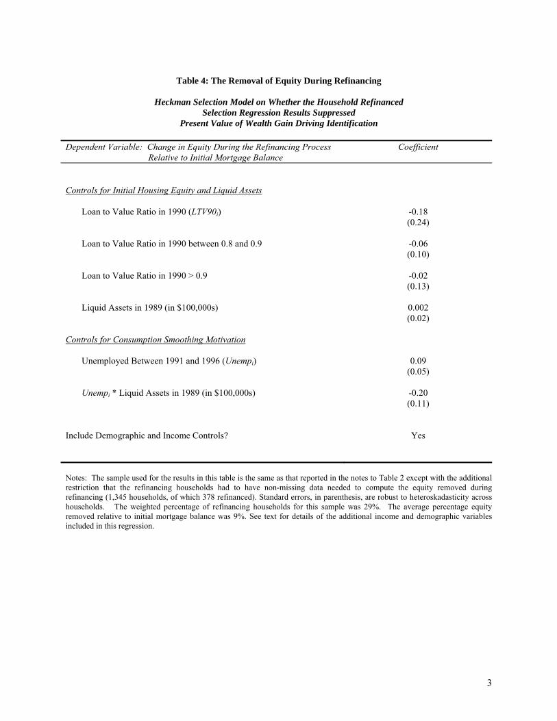
3

Table 4: The Removal of Equity During Refinancing

Heckman Selection Model on Whether the Household Refinanced

Selection Regression Results Suppressed Present Value of Wealth Gain Driving Identification

Dependent Variable: Change in Equity During the Refinancing Process Relative to Initial Mortgage Balance

Coefficient

Controls for Initial Housing Equity and Liquid Assets Loan to Value Ratio in 1990 (LTV90i) -0.18 (0.24) Loan to Value Ratio in 1990 between 0.8 and 0.9 -0.06 (0.10) Loan to Value Ratio in 1990 > 0.9 -0.02 (0.13) Liquid Assets in 1989 (in $100,000s) 0.002 (0.02) Controls for Consumption Smoothing Motivation Unemployed Between 1991 and 1996 (Unempi) 0.09 (0.05) Unempi * Liquid Assets in 1989 (in $100,000s) -0.20 (0.11) Include Demographic and Income Controls? Yes Notes: The sample used for the results in this table is the same as that reported in the notes to Table 2 except with the additional restriction that the refinancing households had to have non-missing data needed to compute the equity removed during refinancing (1,345 households, of which 378 refinanced). Standard errors, in parenthesis, are robust to heteroskadasticity across households. The weighted percentage of refinancing households for this sample was 29%. The average percentage equity removed relative to initial mortgage balance was 9%. See text for details of the additional income and demographic variables included in this regression.

4

Table 5: Interest Rates Paid By Refinancing Households

Heckman Selection Model on Whether the Household Refinanced Selection Regression Results Suppressed

Present Value of Wealth Gain Driving Identification Dependent Variable: Interest Paid By Refinancing Households, Reported by

Household in 1996 Coefficient

Dummy: Year Household Refinanced 1992 -0.42 (0.19) 1993 -0.55 (0.16) 1994 -0.79 (0.16) 1995 -0.47 (0.19) 1996 -0.54 (0.28) Controls for Default Risk of the Refinancing Household Unemployed Between 1991 and 1996 0.41 (0.17) Experience Financial Distress Between 1991 and 1996 0.37 (0.16) Have an Ex-Post Refinancing Loan to Value Ratio Between 0.8 and 0.9 0.22 (0.15) Have an Ex-Post Refinancing Loan to Value Ratio Above 0.9 0.50 (0.20) Include Household Income and Demographic Controls? Yes Include Additional Loan Characteristics? Yes Notes: The sample used in this table is the same as that reported in the footnote to Tables 2 except with the additional restriction that the refinancing households had to report a positive, non-missing value for their interest rate (1,364 households, of which 420 refinanced). Standard errors, in parenthesis, are robust to heteroskadasticity across households. The weighted percentage of refinancing households for this sample was 32%. The average interest rate paid by refinancing households was 7.8%. See the text for details of the additional income and demographic variables and the additional loan characteristics included in this regression.

5

Table 6: Means of Income, Demographic and Wealth Variables for Liquidity Constrained Refinancers and all other Refinancers

Variable Liquidity

Constrained Refinancers

All Other

Refinancers

p-value of

difference Demographics Age of Head in 1989 34 40 <0.01 Education Dummy (Head): Less than High School 0.08 0.03 0.15 Education Dummy (Head): Some College 0.24 0.23 0.86 Education Dummy (Head): College or More 0.35 0.45 0.20 Dummy: African American Head 0.07 0.02 0.05 Dummy: Head Married in 1991 0.95 0.86 0.09 Dummy: Become Married 1991 - 1996 0.01 0.01 0.57 Dummy: Become Divorced 1991 - 1996 0.06 0.01 0.02 Income Average Family Labor Income 1991-1995 58,800 57,700 0.85 Unemployment and Financial Distress Dummy: Unemployment Spell 1991-1996 0.17 0.12 0.33 Dummy: Household Experience Financial Distress 1991-1996 0.32 0.19 0.04 Liquid Wealth Median Liquid Wealth in 1989 6,200 12,000 0.08 Mean Liquid Wealth in 1989 21,900 37,300 0.13 75th Percentile of Liquid Wealth in 1989 18,900 37,700 0.09 Total Wealth Median Total Net Worth in 1989 41,900 106,300 <0.01 Mean Total Net Worth 101,600 171,300 0.03 Equity Removed Percent Removing Equity During Refinancing 0.92 0.57 <0.01 Median Equity Removed (Conditional on Removing Equity) 16,000 11,000 0.22 Mean Equity Removed (Conditional on Removing Equity) 43,400 17,200 <0.01 75th Percentile of Equity Removed (Conditional on Removing) 39,000 20,800 0.05 Notes: The sample for this regression includes all homeowners in the PSID who refinanced between 1991 and 1994, who where in the sample continuously from 1989 to 1994, who were less than 60 years of age in 1989, who had a mortgage in 1989 and who did not move between 1989 and 1994. Additionally, the top/bottom 1% of the change in wealth distribution was truncated (305 observations). We define liquidity constrained refinancers as households who started with an ex-ante loan to value ratio less than 0.8 and ended up with an ex-post loan to value ratio in excess of 0.8. The weighted percentage of liquidity constrained households was 14.4%. Liquid Wealth is defined as the sum of stocks, bonds and cash held by the household. See the text for the full definition.

6

Table 7: Average Propensity to Convert Home Equity (APCE) into Consumption I II III Dependent Variable: Change in Household Wealth (including home equity) between 1989 and 1994

APCE for Liquidity Constrained Households

Who Remove Equity While Refinancing Between

1991 and 1994

APCE for Non-Liquidity Constrained Households Who Removed Equity

While Refinancing Between 1991 and 1994

p-value of difference

1. OLS Regression -0.66 0.20 0.05 (0.29) (0.44) 2. Quantile Regression at Median -0.67 -0.03 < 0.01 (0.09) (0.13) Notes: The sample includes all homeowners in the PSID who where in the sample continuously from 1989 to 1994, who were less than 60 years of age in 1989, who had a mortgage in 1989 and who did not move between 1989 and 1994. Additionally, the top/bottom 1% of the change in wealth distribution was truncated (1,626 observations). The dependent variable for the mean and the median regression is the change in wealth (including housing equity) between 1989 and 1994. The coefficients in columns I and II provide estimates of γ1 and γ2, respectively, from equation (11) in the text and measure the change in wealth that occurs after a household removes $1 of equity from their home during refinancing. See the text for the additional income and demographic controls included as regressors. Heteroskadastic robust standard errors are reported in parenthesis for the OLS regressions. The mean and median change in wealth between 1989 and 1994 was, respectively, $96,018 and $39,629. Column III reports he p-value of a one tail test for whether the APCE for liquidity constrained households (column I) is strictly greater than the APCE for non-liquidity constrained households (column II).