household portfolios and implicit risk preference

HOUSEHOLD PORTFOLIOS AND IMPLICIT RISK PREFERENCE

Alessandro Bucciol and Raffaele Miniaci*

Abstract—We derive the distribution of a proxy for the risk tolerance in arepresentative sample of U.S. households. Our measure is deduced fromthe willingness to bear risk as indicated by the variance of returns of eachhousehold’s observed portfolio. The estimates, obtained assuming con-straints on portfolio composition, show substantial heterogeneity acrosshouseholds. We find that risk tolerance falls with age and increases withwealth. Other variables, such as education, gender, race, and householdsize, do not have a significant relation to risk attitude. Our findings arerobust to changes in portfolio definition, asset returns, and sample compo-sition.

I. Introduction

INDIVIDUALS often face problems under uncertainty,and understanding their attitude toward risk is essential

to predict economic behavior. In this paper, we providenew insights on the distribution of risk preferences acrossU.S. households and study the correlation between risk tol-erance and the main household sociodemographic charac-teristics. We estimate risk preferences from the willingnessto bear risk of each household in our sample (Survey ofConsumer Finances, wave 2004), as indicated by the var-iance of the returns of the observed portfolio made of finan-cial, real, and human assets and under various assumptionson portfolio constraints. In the absence of constraints, ourestimate is proportional to the standard deviation of theobserved portfolio returns.

A large body of literature already estimates the distribu-tion of risk preferences from data on wealth allocation. Pre-vious work is based on analysis of the portfolio share heldin risky assets, assuming that the observed share is theresult of a mean-variance optimizing behavior. We departfrom previous work in three directions. The first is metho-dological. We distinguish between observed and mean-variance efficient portfolios. For each household, we con-struct the efficient portfolio with the same variance as theobserved portfolio. The difference between the two portfo-lios may depend on investment mistakes, information costs,inadequate model assumptions (see Campbell, 2006), orbiased estimates of the returns. Our estimate of risk prefer-ence makes this difference as small as possible.

Our remaining departures concern the definition of port-folio. We consider a broad definition, with a distinctionamong deposits (risk-free), bonds, stocks, human capital,and real estate. Earlier studies take into account only finan-cial assets, frequently grouped into one broad risky cate-gory, or financial assets and human capital. We, however,believe that it may be more realistic to account for the dif-ferent asset characteristics and at least distinguish subcate-gories of financial assets. The size of real estate and itsrelated liabilities, furthermore, is not negligible in house-hold portfolios, and ignoring them may bias the analysis,since house price risk generates hedging needs (Flavin &Yamashita, 2002; Pelizzon & Weber, 2008) and crowds outstock holdings (Cocco, 2005).

Finally, we include constraints on efficient portfolioweights. In particular, we assume that the stock of humancapital is fixed and cannot be changed in our static frame-work. Constraints are relevant also for real estate. Indivi-duals indeed hold owner-occupied housing for investmentas well as consumption purposes. Since housing consump-tion demand typically will not equal investment demand, anowner-occupier distorts the housing investment to bring itinto equality with housing consumption. To correct for thepotential bias due to the housing consumption motive, wefollow Flavin and Yamashita (2002) and take the holding of(owner-occupied) residential housing as exogenous. Anoptimizing agent in our problem thus chooses the portfolioallocation conditional on the wealth held in residentialhousing. We complete our analysis including two othertypes of constraint that are likely to hold at the individuallevel. We require that mortgages cannot exceed the value ofreal estate; we also consider short-selling restrictions indeposits, bonds, and stocks. Short selling in financial mar-kets is not prohibited, but it is discouraged by the fact thatproceeds are not normally available to be invested else-where. This is enough to eliminate a private investor withjust mildly negative beliefs (Figlewski, 1981). The inclu-sion of constraints also reduces potential errors in measure-ment of the efficient portfolio (Green & Hollifield, 1992).

Our estimates of the preference parameter show substan-tial heterogeneity across individuals. In our preferred case,we find risk tolerance to correlate negatively with age andpositively with wealth. Our results suggest that education,gender, race, and household size do not play a significantrole once we control for other variables.

An analysis based on household survey portfolio data isdisturbed by unobserved transaction costs, minimum invest-ment requirements, and other market imperfections. Theseissues affect households in different ways; therefore, theheterogeneity we observe in portfolio composition reflectsdifferences in both risk preferences and market conditions.In fact, in our regression analysis, we find a significant

Received for publication July 26, 2008, Revision accepted for publica-tion June 15, 2010.

* Bucciol: University of Verona, University of Amsterdam, and Nets-par; Miniaci: University of Brescia.

An earlier version of this paper circulated as ‘‘Household Portfolios andImplicit Risk Aversion,’’ Netspar DP 07/2008-036, 2008. We are gratefulto the editors and two anonymous referees for their comments and sugges-tions. We further thank Pierluigi Balduzzi, Guglielmo Weber, and theseminar participants at the Universities of Padua, Pavia, and Verona, andthe NASM 2008 and ICEEE 2009 conferences. We gratefully acknowl-edge Financial support from MIUR (PRIN 2005133231_003 and2007AC54X5_002). The usual disclaimers apply.

The supplemental appendix referred to in this article is available onlineat http://www.mitpressjournals.org/doi/suppl/10.1162/REST_a_00138.

The Review of Economics and Statistics, November 2011, 93(4): 1235–1250

� 2011 by the President and Fellows of Harvard College and the Massachusetts Institute of Technology

effect of variables that may proxy financial sophisticationas well as transaction costs. Transaction and entry costs,however, should be less important among wealthier indivi-duals (Calvet, Campbell, & Sodini, 2009). In the subsampleof the 20% wealthiest households, we observe similar corre-lations for demographic and wealth variables and lower orinsignificant correlations for the proxies of financial sophis-tication and transaction costs; this evidence suggests thattransaction costs are not the main driver of our results.

The remainder of this paper is organized as follows. Sec-tion II surveys the literature on risk preferences. Section IIIpresents our framework. Section IV describes our surveydata (Survey of Consumer Finances, wave 2004) and timeseries data (covering quarterly the years 1980–2004). Sec-tion V reports our benchmark estimates for the portfolio ofa representative agent and the distribution of portfolios inthe sample. Section VI shows the main results of a sensitiv-ity analysis on the return time series. Finally, section VIIconcludes. In the appendix, we discuss the link between ourapproach and the certainty equivalent returns, the construc-tion of the portfolios from the survey data, and the estima-tion of the human capital.

II. Previous Findings on Risk Preferences

The analysis of risk preferences from observed choicedata has been running in a number of economic environ-ments, from labor supply decisions (Chetty, 2006) to prop-erty and liability insurances (Szpiro, 1986), from televisionshows (Beetsma & Schotman, 2001) to auto insurance con-tracts (Cohen & Einav, 2007), and in the laboratory (Schu-bert et al., 1999; Choi et al., 2007). The two main strands ofthis literature, however, focus on consumption and invest-ment choices.

One strand is based on nondurable consumption data.According to the consumption-CAPM (capital asset pricingmodel) framework, consumption choices are fully charac-terized by the Euler equation as a function of the choice inthe previous year, market returns, and a household’s speci-fic preference parameters. To obtain an estimate of the riskaversion parameter, one should use panel data sets with along history of household consumption data. Since suchdata sets are not available, two solutions have been adoptedover the years: running the analysis (a) using time series ofmacroeconomic statistics, assuming that there is a represen-tative agent (see Hansen & Singleton, 1983; Mehra & Pres-cott, 1985; Campbell, 2003), and (b) using pseudo-panelscreated from repeated cross-section survey data, groupingtogether individuals belonging to the same birth cohort (seeAttanasio & Weber, 1995; Blundell, Browning, & Meghir,1994). While the estimate of the risk aversion coefficientgenerally comprises between 2 and 7 using pseudo-panels,it can be well above 10 using time series of macroeconomicstatistics.

A second strand of the literature looks at portfoliochoices and is strictly related to our work. According to the

static mean-variance (MV) portfolio framework, the invest-ment in risky assets depends on the expected values and thecovariances of their returns, and the household’s specificrisk preference. Since household survey data on portfoliocomposition are easily available, it is natural to use thisapproach to study the distribution of risk preferences acrosshouseholds. Empirical work in this field usually takes theshare of portfolios allocated to risky assets (as a whole orjust stocks) as proportional to risk tolerance (Cohn et al.,1975; Friend & Blume, 1975; McInish, 1982; Siegel &Hoban, 1982; Morin & Suarez, 1983; Riley & Chow, 1992;& Shaw, 1996).

With the improvement in the accuracy of survey data,researchers have devised hypothetical questions askingrespondents to compare different lotteries. A number ofauthors used the responses to such questions to infer a mea-sure of risk preference for each household (Barsky et al.,1997; Donkers, Melenberg, & Van Soest, 2001; Guiso &Paiella, 2008; Kimball, Sahm, & Shapiro, 2008).

Those who have examined the distribution of risk prefer-ence typically find a rather large heterogeneity, with the para-meter correlating in particular with wealth, age, gender, andeducation. The correlation with wealth, however, dependscrucially on the definition used. Research focusing on finan-cial wealth seems to support a positive link with risk toler-ance (Friedman, 1974; Cohn et al., 1975; Riley & Chow,1992; Shaw, 1996), reflecting the empirical evidence of stockholdings increasing in wealth (see Guiso, Haliassos, & Jap-pelli, 2001). Shaw (1996) focuses on the effect of humancapital and finds from the Survey of Consumer Finances(SCF) data a positive correlation with risk tolerance. Friendand Blume (1975) also find evidence of a positive relationfrom a precursor of the current SCF, but only when owner-occupied housing is excluded from their definition of wealth.Siegel and Hoban (1982) find from the U.S. National Longi-tudinal Survey data patterns consistent with increasing orconstant risk tolerance using narrow definitions of wealth,and patterns consistent with decreasing risk tolerance usingbroader definitions of wealth, including housing and nonmar-ketable assets. Morin and Suarez (1983) draw similar conclu-sions using the Canadian SCF and including human capital inthe definition of wealth. Financial, human, and real holdingsare, however, very different assets with different degrees ofliquidity. One may expect different results from an analysisthat takes into account constraints on portfolio holdings.

In general, there seems to be consensus on the relation ofrisk tolerance, age, gender, and education. The majority ofthe empirical studies have found that risk tolerance reduceswith age (McInish, 1982; Morin & Suarez, 1983; Palsson,1996), is lower for women (see Palsson, 1996; Halek &Eisenhauer, 2001; and the literature review in Croson &Gneezy, 2009), and less highly educated individuals (see inparticular Riley & Chow, 1992; & Halek & Eisenhauer,2001).

It is not clear whether these correlations hold as such orare instead capturing correlations with other variables

1236 THE REVIEW OF ECONOMICS AND STATISTICS

omitted from the analysis. For instance, one might observea correlation between risk preference and education,whereas the true correlation is between risk preference andfinancial sophistication (Guiso & Jappelli, 2005). Theobserved correlation might arise just because more sophisti-cated individuals are also more highly educated on average.With this paper, we aim to shed further light on this issue,using portfolio choice data and considering a richer specifi-cation to include the main demographic, social, and eco-nomic variables of a household.

III. Framework

Our economy includes one risk-free asset and a set of nrisky assets with vector of expected excess returns g andcovariance matrix S; (e, S) consistently estimate the trueasset return moments (g, S).

For each household i(i ¼ 1,. . .,N) with its specific risktolerance (RT) coefficient ci, we compute the MV-efficientportfolio of weights wi cið Þ ¼ wi;1 cið Þwi;2 cið Þ ...½ wi;n cið Þ�0.We assume that the household’s observed portfolio ofweights, xi ¼ xi;1 xi;2 . . . xi;n½ �0, proxies the efficientone of weights wi(ci). In other words, we allow theobserved portfolio to deviate from the efficient one forinvestment mistakes, market imperfections, or incompleteinformation about the household’s risk type. More trivially,the two portfolios may differ because of incorrect estimatesof (e, S) or inadequate model assumptions.

Our RT estimate is the value of ci implicit in the follow-ing equation, which imposes an identity in the variance ofthe returns on the two portfolios:

wi cið Þ0Swi cið Þ ¼ x0iSxi: ð1Þ

Figure 1 shows our metric in a mean-standard deviationplan. With our approach, we compare portfolios A and B.One could argue, however, that there is no specific reasonto look at portfolio variances; we could also look at, for

instance, portfolio expected returns. In this case, we wouldcompare portfolios A and C of the figure. More generally,any portfolio along the efficient frontier is a potential candi-date for our comparison. It is important to notice that effi-cient portfolios with lower (higher) variance of returns thanthe observed portfolio have a larger (smaller) holding ofrisk-free assets than the efficient portfolio we consider.Using them in the comparison would therefore generate alower (higher) RT estimate. However, we believe that thevariance of an observed portfolio is a stronger indicator ofthe household’s willingness to bear risk. There are twofurther reasons that one may want to look at the portfoliovariance. First, the variance is more robust to estimationerrors than the expected return (Merton, 1980; Chopra &Ziemba, 1993); second, our approach is consistent with theanalysis in terms of certainty equivalent returns (CER) fromstandard expected utility theory (as in Calvet et al., 2009;see section A1 in the appendix).

We call ‘‘expected return gap’’ the difference in theexpected returns of the two portfolios,

qi ¼ e0 wi cið Þ � xið Þ: ð2Þ

This statistic has at least four possible interpretations. Itcan be seen as the lower bound of the optimization bias,incurred when choosing the observed portfolio xi ratherthan its efficient alternative wi due to investment mistakes,the lack of rationality, or the lack of financial sophistica-tion. The gap may also indicate the cost of market imper-fections, in which agents deviate from the optimal behaviorbecause of transaction or information costs. Third, the gapmay inform on the imprecision in the estimate of the effi-cient portfolio due to errors in the asset moments. A finalpossible interpretation is a measure of how close our frame-work is to the actual behavior.

It is well known that in the absence of constraints in port-folio composition, the efficient weights are given by theequation

wi ¼ ciS�1e; ð3Þ

in which case the expected return gap is

qi ¼ e0S�1e� �1=2

x0iSxi

� �1=2�x0ie: ð4Þ

Substituting equation (3) in equation (1), we solve the iden-tity for ci and obtain that risk tolerance is proportionalto the standard deviation of the returns on the observedportfolio:

ci ¼x0iSxi

e0S�1e

� �12

: ð5Þ

Investors, however, usually face constraints to their port-folio allocation. We consider equality and inequality con-straints on portfolio composition, described for a genericportfolio of weights x by the conditions

FIGURE 1.—METRIC USED FOR RT ESTIMATION

1237HOUSEHOLD PORTFOLIOS AND IMPLICIT RISK PREFERENCE

Ax ¼ b; ð6Þ

Cx � d: ð7Þ

In general, the problem has no closed-form solution, andthe solution is found numerically with quadratic program-ming.1 A closed-form solution to our problem is availableonly under equality constraints (6). In this case, it turns outthat the efficient portfolio has weights

wi ¼ ciQþ q ð8Þ

with

Q ¼ I � S�1A0 AS�1A0� ��1

A� �

S�1e

q ¼ S�1A0 AS�1A0� ��1

b;ð9Þ

and we estimate risk tolerance from

c2i ¼

q0Sq� x0iSxi

Q0SQ� 2Q0e: ð10Þ

This measure is strictly positive as long as b = 0. To get anintuition, consider the simple case of constraints requiringthat a subset xe of f weights is fixed, that is, x0 ¼ x0u x0c½ �,and equation (6) rewrites as

Ax ¼ 0f� n�fð Þ

Ifh i

xu

xc

� ¼ xc; ð11Þ

where If is an f � f identity matrix. In this case, the optimalweights are given by

wi ¼wi;u

wi;c

� ¼ ci Suuð Þ�1eu � Suuð Þ�1Sucxc

xc

� ; ð12Þ

with eu and Suu expected excess returns and the covariancematrix of the unconstrained assets, and Suc the covariancematrix between unconstrained and constrained assets. Effi-cient allocation of the unconstrained portfolio weightsaccounts for an additional hedge term S�1

uu Sucxc depending onthe variance of the unconstrained assets, the covariance be-tween unconstrained and constrained assets, and the holdingof constrained assets xc. Notice that equation (12) is indepen-dent of the expected excess returns and the variance of theconstrained assets. A household with holdings only in risk-freeand constrained assets has in this framework a positive RTcoefficient, because it does not make further investments tohedge against the risk associated with the constrained wealth.

IV. Data

A. Household Portfolios

In order to estimate the risk tolerance parameter withinthe framework we have described, we need detailed infor-

mation on wealth allocation for a representative sampleof households. Banks and fund managers may providedetailed data on their customers’ financial portfolios, butusually these data sets are not representative of the wholepopulation. Furthermore, they typically ignore human capi-tal and real estate, which are likely to influence house-holds’ decisions. An obvious candidate data set for our pur-pose is the U.S. Survey of Consumer Finances (SCF), arepeated cross-sectional survey of households conductedevery three years on behalf of the Federal Reserve Board.It collects detailed information on assets and liabilities,including home ownership and mortgages, together withthe demographic characteristics of a sample of U.S. house-holds. The survey deliberately oversamples relativelywealthy households to produce more accurate statistics;sampling weights are then provided to obtain unbiased sta-tistics for the U.S. population. The SCF also handles thehigh rate of item nonresponse typical of wealth-relatedmicrodata by imputing a set of five values that represent adistribution of possibilities. Multiple imputations of miss-ing data increase the efficiency of estimation, allowing theresearcher to use all available information, and have thedistinct advantage of providing information on uncertaintyin the imputed values. We exploit this information as sug-gested in Rubin (1987); we develop our analysis indepen-dently for each of the five completed data sets, and ourfinal statistics are the average of the estimates derived foreach data set.

Our data on household portfolio holdings are taken fromwave 2004 of the SCF (4,519 observations). We considertwo definitions of portfolio. The narrow definition includesthe main financial assets, which we aggregate in three cate-gories: deposits, bonds, and stocks. The broad definitionalso includes human capital, real estate, and their relatedliabilities, plus two more categories: human wealth and realestate. From the sample, we drop households with missinginformation on financial wealth (296 cases) or income (103cases) and the households whose portfolios do not meet theconstraints we define in section IVB (25 cases). Our finalsample consists of 4,095 households.

The distribution of household wealth changes markedlyusing either definition—narrow or broad (table 1). Whilewe find a median value of $11,000 using the narrow defini-tion, the median is $52,338 using the broad definition netof human capital (and $141,300 also including humancapital).

Each asset is classified as defined in table 1 (for detailson the calculation of portfolio see section A2). Table 1 alsoreports the composition of the aggregate portfolio, com-puted accounting for multiple imputations and samplingweights. We observe that most financial wealth is held instocks. Considering our broad definition, the largest shareof wealth (52%) is held in real estate, mostly in owner-occupied residential housing (39%). The inclusion of mort-gages in the bonds class determines an aggregate short posi-tion in it.1 We use the function quadprog in Matlab.


B. Portfolio Constraints

We analyze three situations: one using the narrow portfo-lio definition (only financial assets) without constraints (theunconstrained narrow definition) and two using the broaddefinition (financial assets plus human wealth plus realestate). In one case, we consider only equality constraintson human capital, that is, we assume that human capital isfixed for portfolio decisions (with a little imprecision of ter-minology, we call this the unconstrained broad definition).In the second case (the constrained broad definition), wealso consider short-selling constraints on the financial com-ponents and equality constraints on residential housing.Specifically, our constraints are fixed holding of humancapital; no short sale in deposits, bonds, and stocks; nomortgage financing for more than the value of real estate

(that is, bonds cannot take a position below the opposite ofreal estate); and investment in real estate not lower than thevalue of residential housing. We include constraints onhousing to deal with a potential consumption motive thatdrives the investment in residential housing. To limit thiseffect, Pelizzon and Weber (2009) adjust household portfo-lios, reducing real estate holdings by an imputed presentvalue of future rents. In our static framework, we insteadfollow Flavin and Yamashita (2002) and Pelizzon andWeber (2008) and assume that households choose the allo-cation of wealth conditional on their holding of residentialhousing.

C. Asset Time Series

We take annual financial returns (bonds and stocks) fromthe Merrill Lynch U.S. Corporate & Government MasterIndex and MSCI USA Stock Index time series of U.S. assettotal return indices (downloaded from Datastream). Weconsider as risk-free return the yield of three-month T-bills.To measure the uncertainty related to human capital, weconstruct from U.S. Bureau of Economic Analysis (BEA)data a time series of labor income consistent with the defini-tion we used in the SCF.2 Our time series cover quarterlythe years from 1980 to 2004 (100 observations). To com-pute the correlations with the asset excess returns, we sub-tract from this series the series of our risk-free returns.

It is more problematic to find a time series of real estatereturns valid for our purpose. From the perspective of ahousehold, we need a series that accounts for not only capi-tal gains but also earnings due to rents. This information isnot available in standard indices such as OFHEO and S&P/Case-Shiller home price indices. We therefore use the MIT-CRE Transaction-Based Index of U.S. Real Estate Invest-ment. This index, measured since 1985 on a quarterly fre-quency, is based on transaction prices to avoid sources ofindex smoothing and lagging bias that are present in otherindices (Fisher, Geltner, & Pollakowski, 2007). The totalreturn index we consider incorporates returns from propertyvalue and from property cash flow in the apartment, indus-trial, office, and retail sectors.

We compute excess returns as returns net of the yieldreturn of the risk-free asset. When we use the largest periodavailable for all the series (1985–2004 on a quarterly fre-quency), bonds dominate real estate returns in a mean-variance sense. As a consequence, no mean-variance optimi-zer would hold a long position in real estate, in contrast tomost of the portfolios we observe in the SCF sample. Toovercome this problem, one possibility is to consider ashorter period length; this case is discussed in section VIA.

TABLE 1.—AGGREGATE WEALTH AND PORTFOLIO COMPOSITION (% FROM SCF,2004)

Definition

Category Narrow Broad

Wealth25th percentile $1,538 $70,46350th percentile $11,000 $141,30075th percentile $59,000 $256,692Mean $169,484 $475,687

Portfolio compositionChecking accounts 5.388 1.918Savings and money market accounts 8.766 3.120Call accounts at brokerages 1.255 0.447IRA-Keogh accounts 2.270 0.808Retirement accounts 0.803 0.286Annuities 0.914 0.326Trust-managed accounts 1.360 0.484

Deposits 20.756 7.388Certificates of deposits 4.326 1.540Savings bonds 0.655 0.233Directly held corporate bonds 6.116 2.177Tax-free mutual funds 1.694 0.603Government bond mutual funds 0.520 0.185Other bond mutual funds 1.060 0.377½ balanced mutual funds 0.640 0.228½ other mutual funds 0.559 0.199IRA-Keogh accounts 5.805 2.066Retirement accounts 0.800 0.285Annuities 0.874 0.311Trust-managed accounts 1.734 0.617Life insurances (cash value) 3.450 1.228Mortgages on primary residence (-) — �11.100Lines of credit on primary residence (-) — �0.350Loans on other real estate (-) — �2.717

Bonds 28.231 �4.119Directly held stocks 20.670 7.357Stock mutual funds 11.531 4.104½ balanced mutual funds 0.640 0.228½ other mutual funds 0.559 0.199IRA-Keogh accounts 11.311 4.026Retirement accounts 1.899 0.676Annuities 1.294 0.460Trust-managed accounts 3.109 1.106

Stocks 51.013 18.156Owner-occupied primary residence — 38.574Other real estate — 13.725

Real estate — 52.299Human capital — 26.276

Number of observations: 4,095. For an explanation of the italicized terms, see section A2 in theappendix.

2 See section A2 in the appendix. We take the difference between perso-nal income and earnings from rents, dividends, and capital gains. Theresulting time series incorporates wage and salary disbursements, supple-ments to wages and salaries, proprietors’ income with inventory valuationand capital consumption adjustments, and personal current transferreceipts, less contributions for public social insurance.


In our benchmark case, we instead extend our time serieslength using the method suggested in Stambaugh (1997).We exploit the same-period correlation between financialand real asset returns to predict prior realizations of realasset returns from observations of financial asset returnsdating back to 1980. Our final series cover the period 1980to 2004 (100 observations) on a quarterly frequency and areshown in figure 2; the asset moments are computed accord-ing to Stambaugh (1997) and reported in table 2, panels Aand B. Stocks are by far the category with the highest riskand expected excess return; their Sharpe ratio is, however,below the one of bonds (30% instead of 43%). Since in ouranalysis we always take the holding of human capital asfixed, the historical return on income and its variance donot matter for the computation of the efficient portfolio orRT; what matters is only its correlation with the returns onthe other assets.3 Similarly, under our constrained broaddefinition, the historical return on real estate and its var-iance matters only for the portfolio choice between financialassets and real estate assets except for the primary resi-dence.

Panel C of table 2 shows two optimal portfolios arisingfrom these moments. Under the narrow definition, we takethe tangency portfolio, and under the broad definition, wecompute the efficient portfolio that fulfills equation (12)with the constraint that the weight on human capital is equalto the value observed in the aggregate portfolio; we use avalue of c such that the weights on all the risky assets sumto 1. This latter portfolio is more consistent in our analysisthan the tangency portfolio under the broad definition, aswe always keep human capital fixed. Under our narrowdefinition, an efficient allocation of wealth would prescribean investment in bonds 78.91/21.09 ¼ 3.74 times as large

as an investment in stocks—a number sizably differentfrom the 28.23/51.01 ¼ 0.55 ratio observed in the aggregateportfolio. A similar picture emerges from the optimal port-folio under the broad definition. With respect to the aggre-gate observed portfolio, the MV strategy would suggestincreasing the investment in stocks and real estate and (con-sequently) reducing indebtness.

V. Benchmark Results

A. Risk Tolerance for a Representative Agent

We first present a measure of risk tolerance for a repre-sentative agent in our sample. We derive the RT coefficientand the expected return gap using as observed portfolio theaggregate portfolio (whose average over the five imputa-tions is shown in table 1).

The first two columns of table 3 show our estimatestogether with confidence intervals based on 1,000 bootstrapsimulations over the household units. We obtain an RTcoefficient of 0.21 from the financial portfolio definitionand 0.12 and 0.37, respectively, from the unconstrained andconstrained broad portfolio definitions. The frameworkusing the unconstrained broad portfolio definition is the clo-sest to the one in the consumption-CAPM literature, as ittakes into account an exogenous measure of income anddoes not impose any constraint on the other asset cate-gories. Our estimate implies a risk aversion of 1/0.124 ¼8.065, which is in the lower bound of the range of estimatesreferring to the consumption-CAPM and based on time ser-ies. In all the other cases, we obtain sizably smaller esti-mates of risk aversion (4.73 under the narrow definition and2.71 under the constrained broad definition), which aremore in line with the microeconometric evidence.

The second column of table 3 reports the expected returngap of the representative agent and its confidence interval

FIGURE 2.—HISTORICAL EXCESS RETURNS, 1980–2004

Note: Real estate returns before 1985 are imputed according to Stambaugh (1997).

TABLE 2.—EXCESS RETURN TIME SERIES STATISTICS

Bond StockReal

EstateHumanCapital

A: Historical Excess Returns (%)a

Asset CategoryMean 3.730 5.319 2.286 0.401S.D. 8.71 17.624 7.878 2.492Sharpe ratio 42.775 30.182 29.018 16.074

B: Covariances and Correlations (%)b

AssetBond 0.760 26.743 25.859 15.316Stocks 0.411 3.106 30.605 16.668Real estate 0.178 0.425 0.621 46.083Human capital 0.033 0.073 0.091 0.062

C: Optimal Portfolios (%)c

Portfolio definitionNarrow 78.914 21.086 - -Broad 45.004 10.517 18.203 26.276

aRisk-free historical return: 5.932%.bCorrelations in italics.cNarrow definition: tangency portfolio. Broad definition: efficient portfolio with equality constraint on

the human capital weight, and weights on risky assets summing to one.

3 Importantly, this implies that idiosyncratic income risk is not relevantin our framework.


based on the same bootstrap simulations as for the risk tol-erance. The return gap is 0.90% per year under the narrowdefinition and 0.89 (0.50) under the unconstrained (con-strained) broad definition. The gap of the narrow definitionis not directly comparable with the gap of the broad defini-tion (either constrained or not) because of the different defi-nitions of wealth they refer to. We can instead interpret thedifference 0.89 � 0.50 ¼ 0.39 as the annual percentage costof facing constraints in real and financial wealth allocationunder the broad definition.

B. Risk Tolerance for Each Household

Focusing on the representative agent can be misleadingbecause households may have very different preferences.We therefore investigate the heterogeneity in our sample byestimating the risk tolerance implicit in the portfolio of eachhousehold in our data set.

When we compute the statistic for each observation inour sample, the median RT values are 0.08, 0.12, and 0.14,respectively, using for the portfolio financial definition theunconstrained and constrained broad definitions (third col-umn of table 3). Table 3 also reports below each point esti-

mate the 2.5% and 97.5% quantiles of the sample distribu-tion of the estimates. Only in the case of unconstrainedbroad portfolio definition do we obtain a median risk toler-ance close to the aggregate portfolio; in all the remainingcases, values are around 60% smaller. However, the size ofthe coefficient varies widely across the households. Figure 3,panel A, reports the empirical cdf of our RT estimates,under the constrained broad definition, together with a non-parametric 95% confidence interval (Wasserman, 2006).Under the narrow definition, we estimate an RT of 0 for1,162 households (36.65% of the sample once we accountfor sampling weights); when we ignore such households,the median RT in the sample becomes 0.17. In contrast, RTis always positive under the broad definition, because house-holds hold at least deposits and human capital. Consider ahousehold with only deposits and human capital. In thiscase, our approach estimates ci > 0 because the householddoes not hedge against the risk associated with income vola-tility (see equation [12]).

Our estimates of RT vary according to the underlyingassumptions on the assets space and the constraints and aregenerally little correlated; in particular, the correlationbetween estimates under the narrow and constrained broad

TABLE 3.—SUMMARY STATISTICS

Representative Agent Household-Specific (Median)

Portfolio Definition Risk ToleranceExpected

Return Gap (%) Risk ToleranceExpected

Return Gap (%)

Narrow, unconstrained 0.211 0.903 0.080 0.116(0.203, 0.219) (0.817, 0.991) (0, 0.345) (0, 2.669)

Broad, unconstrained 0.124 0.888 0.115 0.992(0.122, 0.127) (0.843, 0.935) (0.022, 0.286) (0.080, 7.389)

Broad, constrained 0.368 0.500 0.142 0.044(0.346, 0.390) (0.468, 0.535) (0.008, 0.933) (0, 1.357)

In parentheses: Representative agent: 95% confidence interval based on 1,000 bootstrap simulations over the household units. From each simulation, we compute the aggregate portfolio using the sampling weights,and separately for the five imputations. Household specific: 2.5% and 97.5% quantiles of the empirical distribution.

FIGURE 3.—EMPIRICAL CUMULATIVE DISTRIBUTIONS

A: Risk ToleranceB: Expected Return Gap


portfolio definitions is just 0.076. Risk tolerance increasesfor 1,850 households (55.76% of the sample once weaccount for sampling weights) when we consider the broadrather than the narrow definition of portfolio, and itincreases for 2,468 households (53.96% of the sample)when we take into account constraints in our broad portfoliodefinition. In this latter case, households with larger risk tol-erance are wealthier, hold larger portfolio weights on hous-ing, resort to mortgages more heavily, and use this addi-tional wealth to finance their investment in stocks.

We obtain similar findings for the expected return gap(the last column of table 3). While the median gap underthe unconstrained broad portfolio (0.99% per year) isroughly comparable to the aggregate one, the median gapsin the other two cases (0.12% and 0.04% under the narrowand constrained broad definitions) are considerably smaller(last column of table 3). The empirical cdf in figure 3, panelB, further suggests that the expected return gap is negligiblefor most households under the constrained broad definition.We interpret this evidence as indicative that our frameworkfits the observed behavior better when real and humanwealth are considered but subject to constraints.

The reasonableness of our estimates is confirmed by thecomparison with the response to a question asked of all thesubjects in the SCF sample:

Which of the following statements comes closest todescribing the amount of financial risk that you [andyour husband/wife/partner] are willing to take whenyou save or make investments?

1. Take substantial financial risks expecting to earn sub-stantial returns

2. Take above-average financial risks expecting to earnabove average returns

3. Take average financial risks expecting to earn averagereturns

4. Not willing to take any financial risks

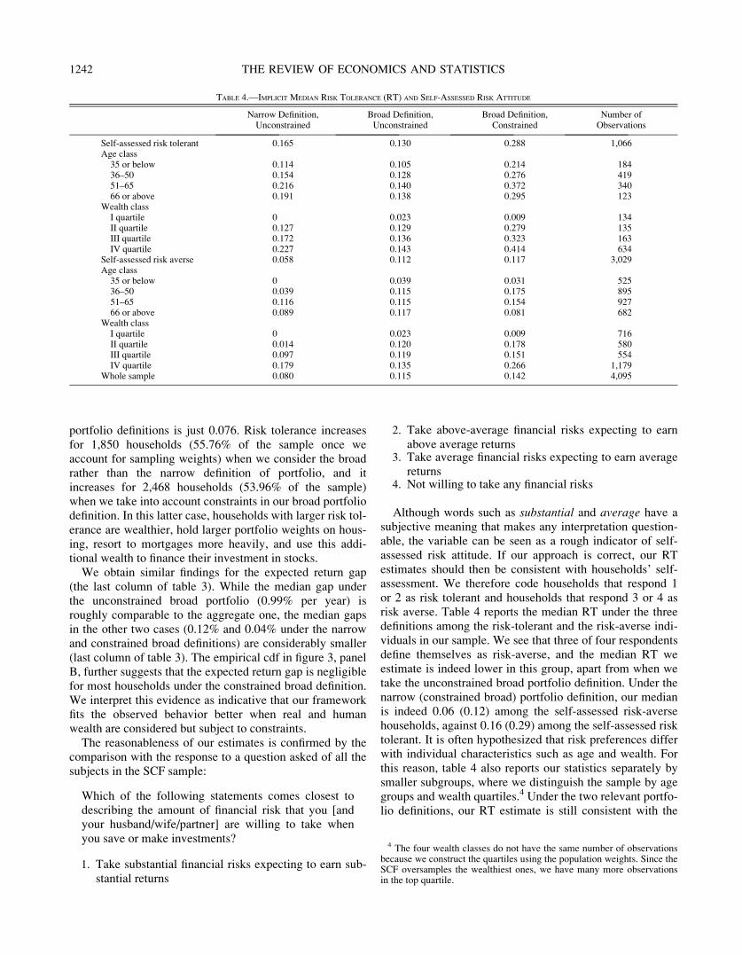
Although words such as substantial and average have asubjective meaning that makes any interpretation question-able, the variable can be seen as a rough indicator of self-assessed risk attitude. If our approach is correct, our RTestimates should then be consistent with households’ self-assessment. We therefore code households that respond 1or 2 as risk tolerant and households that respond 3 or 4 asrisk averse. Table 4 reports the median RT under the threedefinitions among the risk-tolerant and the risk-averse indi-viduals in our sample. We see that three of four respondentsdefine themselves as risk-averse, and the median RT weestimate is indeed lower in this group, apart from when wetake the unconstrained broad portfolio definition. Under thenarrow (constrained broad) portfolio definition, our medianis indeed 0.06 (0.12) among the self-assessed risk-aversehouseholds, against 0.16 (0.29) among the self-assessed risktolerant. It is often hypothesized that risk preferences differwith individual characteristics such as age and wealth. Forthis reason, table 4 also reports our statistics separately bysmaller subgroups, where we distinguish the sample by agegroups and wealth quartiles.4 Under the two relevant portfo-lio definitions, our RT estimate is still consistent with the

TABLE 4.—IMPLICIT MEDIAN RISK TOLERANCE (RT) AND SELF-ASSESSED RISK ATTITUDE

Narrow Definition,Unconstrained

Broad Definition,Unconstrained

Broad Definition,Constrained

Number ofObservations

Self-assessed risk tolerant 0.165 0.130 0.288 1,066Age class

35 or below 0.114 0.105 0.214 18436–50 0.154 0.128 0.276 41951–65 0.216 0.140 0.372 34066 or above 0.191 0.138 0.295 123

Wealth classI quartile 0 0.023 0.009 134II quartile 0.127 0.129 0.279 135III quartile 0.172 0.136 0.323 163IV quartile 0.227 0.143 0.414 634

Self-assessed risk averse 0.058 0.112 0.117 3,029Age class

35 or below 0 0.039 0.031 52536–50 0.039 0.115 0.175 89551–65 0.116 0.115 0.154 92766 or above 0.089 0.117 0.081 682

Wealth classI quartile 0 0.023 0.009 716II quartile 0.014 0.120 0.178 580III quartile 0.097 0.119 0.151 554IV quartile 0.179 0.135 0.266 1,179

Whole sample 0.080 0.115 0.142 4,095

4 The four wealth classes do not have the same number of observationsbecause we construct the quartiles using the population weights. Since theSCF oversamples the wealthiest ones, we have many more observationsin the top quartile.


self-assessed measure and is always lower among the risk-averse households. Only in the lowest wealth quartile do wenot observe a clear difference between self-assessed risk-tolerant and self-assessed risk-averse individuals, as our RTestimates are tiny for both.

C. Heterogeneity in Risk Preferences

To further investigate the heterogeneity of risk tolerancein the population, we perform an OLS regression analysisand examine the potential correlations between our RTmeasure and the economic and demographic characteristicsof the households (table 5). Our dependent variable isln 1þ cið Þ, where ci is the RT coefficient of household i,i ¼ 1,. . ., N estimated from the unconstrained narrow port-

folio definition, and the unconstrained or constrained broadportfolio definition. The regression equation includes age;the logarithm of income; the logarithm of wealth net ofhuman capital (either the narrow or broad definition, consis-tently with the dependent variable); a dummy variableequal to 1 if children are present in the household; anddummy variables for the gender, marital status (divorced,widowed, never married), race, education (high schoolgraduate, college graduate), and occupational status(employed, self-employed) of the household head.5 This

TABLE 5.—HETEROGENEITY OF RISK TOLERANCE

Narrow Definition,Unconstrained

Broad Definition,Unconstrained

Broad Definition, constrained

Whole sample Top 20% wealth

Age/100 �2.206 �5.604*** �17.454*** �40.187***(1.389) (1.072) (5.076) (11.607)

ln(income)/10 �5.477** �14.896*** �5.139 �36.467**(2.274) (1.722) (7.968) (15.541)

ln(wealth)/10 22.390*** 16.156*** 29.872*** 72.741***(0.744) (0.620) (2.843) (13.505)

With children �0.054 0.360 �1.258 �2.565(0.350) (0.250) (1.460) (2.150)

Female 0.085 �0.023 �4.428 �7.217*(0.521) (0.508) (3.689) (4.245)

Divorced 0.618 1.073** 8.792*** 0.886(0.556) (0.455) (2.923) (3.560)

Widowed �0.025 0.432 7.253 3.834(0.765) (0.674) (5.312) (5.462)

Never married 0.327 �0.951* 3.514 �.2.048(0.582) (0.529) (3.385) (5.544)

Nonwhite �0.689* 0.077 �0.328 �2.139(0.379) (0.307) (1.748) (3.014)

High school graduate 0.195 �0.309 0.756 �3.211(0.864) (0.749) (2.168) (12.650)

College graduate 0.948 �0.056 3.104 1.995(0.879) (0.797) (2.846) (12.601)

Employed �0.283 0.546 0.590 �3.208(0.478) (0.338) (1.398) (3.070)

Self-employed �0.822 0.012 2.849 �2.686(0.597) (0.386) (2.935) (3.229)

With financial adviser 0.268 �0.005 0.279 0.228(0.337) (0.218) (1.334) (1.804)

Works in finance sector 0.747 �0.482 3.238 2.362(0.575) (0.381) (3.014) (3.495)

Shops around for best rates on credit 0.790** 0.470** 3.546** 0.850(0.320) (0.235) (1.395) (1.982)

Uses a computer to manage money 0.592 0.258 4.867** 5.366**(0.410) (0.275) (1.972) (2.161)

Number of financial institutionswhere doing business

0.239*** 0.214*** 1.524*** 0.930**(0.066) (0.044) (0.357) (0.425)

Self-assessed good health �0.219 0.330 2.999* 0.937(0.357) (0.258) (1.608) (2.081)

Optimistic about future 0.512 0.120 0.599 0.687(0.310) (0.230) (1.427) (1.849)

Constant �6.311*** 10.298*** �9.652 �8.111(2.369) (1.881) (8.196) (24.968)

Number of observations 4,095 4,095 4,095 1,602Multiple imputation minimum dof 89.0 146.8 122.3 92.4RT (c) average household 0.101 0.113 0.239 0.373

The dependent variable is ln(1 þ c); all parameters and standard errors are multiplied by 100. Robust standard errors in parentheses. Method: OLS. ‘‘RT (c) average household’’ is computed as

exp ln 1þ cð Þn o

� 1 where ln 1þ cð Þ is the sample average. ***Significantly different from 0 at 1%, **5%, *10%.

5 Using a specification with a quadratic polynomial on age, we pre-dicted a linear age-risk tolerance profile in the relevant age range.Although in the following we discuss age effect, it should be noted thatwith these data, we cannot disentangle age and cohort effects.


specification is similar to the one in Sahm (2007), who esti-mates RT from hypothetical questions in the U.S. Healthand Retirement Study.6 In the same vein as Guiso andJappelli (2005), we further include in the specification someproxies for financial sophistication: the number of financialinstitutions the household is involved with and a set offour dummy variables. The dummies are worth 1 if there isregular consulting with professional financial adviser, thehead works in the finance sector, the household shopsaround for best rates on credit and borrowing, or the house-hold uses a computer to manage money. We also include adummy variable for the self-assessed good or excellenthealth status of the head. Following Ben Mansour et al.(2008), who find a negative correlation between risk toler-ance and optimism, we finally include in the specification avariable denoting the self-assessed degree of optimism ofthe household.7

The first three columns of table 5 report the output of thisregression using the three RT estimates and the full sampleof households available. Note that under the narrow portfoliodefinition, the dependent variable ln 1þ cið Þ coincides with

ln 1þ x0iSxi=e0S�1e� �1=2

� �, where x0iSxi is the variance of

the returns of the observed portfolio held by household i. Inthe absence of constraints, indeed, cross-sectional differ-ences depend on only the variance of the observed portfolioreturns, which is more robust to estimation errors than theexpected return (Merton, 1980; Chopra & Ziemba, 1993).

There is no consensus in the literature on how risk toler-ance should vary with wealth; Siegel and Hoban (1982) andMorin and Suarez (1983) found for risk aversion a negativecorrelation with narrow definitions of wealth (financial) anda positive correlation with broader definitions of wealth(also including real and nonliquid assets). In all our regres-sions, we find wealth to be positively correlated with risktolerance at a 1% significance level. Given our functionalform, the elasticity of risk tolerance to wealth is equal tothe coefficient of ln(Wealth) times the ratio (1 þ ci)/ci. Let

ln 1þ cið Þ be the dependent variable sample average. If wetake as a reference the average household, for which

~c ¼ exp ln 1þ cið Þn o

� 1, the estimated elasticity ranges

between 0.155 of the constrained broad definition and 0.245of the financial portfolio. As wealth moves from the 25th tothe 75th percentile (see table 1), the predicted variation

amounts to 17% of the corresponding interquar-

tile distance in the case of constrained broad definition (seetable 4); this percentage rises to 50% in the case of thefinancial portfolio. (Log) income is negatively partially cor-

related with (log) risk tolerance in the unconstrained casesbut not in the broad constrained one. When human capitaland real estate are considered, we estimate a significantpositive effect of being divorced and a negative effect ofage. However, a clear limitation of this analysis is that wecannot separate age from cohort effects.

The proxy variables for financial sophistication prove tobe correlated with risk tolerance. In particular, in all of thecases, our estimate shows that households using a largernumber of financial institutions and those shopping aroundfor better credit conditions are characterized by higher risktolerance; when we consider the constrained broad defini-tion, households that use a computer to manage their moneyare significantly more risk tolerant. Consulting or not afinancial adviser is not correlated with the degree of risktolerance, nor is being optimistic or pessimistic about futureeconomic conditions.

After having controlled for income, wealth, and financialsophistication, our estimates show a negative correlationbetween risk tolerance and age, but only when human capi-tal and real estate are included in the definition of portfolio.We find instead no direct effect of gender and education onrisk tolerance, and only in the case of financial portfolio isthere weak evidence in favor of the hypothesis that non-white households are less risk tolerant than average. Wealso tried a specification including two self-assessed mea-sures: risk attitude and time horizon. The first is the answerto the question discussed at the end of section VB; the sec-ond is the answer to a question on ‘‘the horizon consideredfor planning saving and spending.’’ The regression output(available in the online supplementary appendix), however,does not change in any noticeable way, and we omit thetwo measures from our preferred specification.

Our interpretation of the results relies on the assumptionthat the heterogeneity in cross-sectional holdings is mainlydue to preference heterogeneity rather than transactioncosts. In fact, small and heterogeneous transaction costsmay be sufficient to generate infrequent portfolio adjust-ment, resulting in a large dispersion of portfolio composi-tions even across households with identical risk prefer-ences. The existing evidence on household trading ismixed. Research on brokerage accounts finds evidence ofintense trading activity (Odean, 1999; Barber & Odean,2000), while research on retirement plans (Madrian & Shea,2001; Agnew, Balduzzi, & Sunden, 2003), portfolio man-agement (Alessie, Hochguertel, & Van Soest, 2004), andequity market participation (Vissing-Jorgensen, 2002) findssubstantial inertia. King and Leape (1998) suggest thatthere is a significant holding cost (due to transaction andinformation motives) in the management of a portfolio,which induces investors to hold incomplete and suboptimalportfolios. These costs may surpass the forgone gains thatcould be obtained with a better-structured portfolio.

Direct information on the transaction costs that eachhousehold faces is, of course, not available. To some extent,we might expect that our proxy variables for financial

6 Sahm (2007) focuses on cash on hand (wealth plus income) rather thanwealth. We prefer our specification because cash on hand is highly corre-lated with income. For the same reason, we do not consider a measure oflife cycle wealth as described by the sum of wealth and human capital.

7 The question asks whether ‘‘the US economy will perform better,worse, or about the same in the next 5 years.’’ We consider optimisticthose who report ‘‘better.’’


sophistication also capture part of the heterogeneity intransaction costs that households face. Previous research,however, suggests that transaction costs are less importantfor wealthier individuals, who make more frequent portfolioadjustments. This view is consistent with a fixed element oftransaction costs (Agnew et al., 2003; Calvet et al., 2009).Hence, as a robustness check, we perform our analysis onthe subsample of the households whose wealth is in the top20% of the weighted distribution in our sample. These aremore than 20% of the observations in our sample, becausethe SCF oversamples wealthier households. This subsampleis remarkably different from the full sample not onlybecause it is richer (and consequently more risk tolerant onaverage), but also because it includes fewer female heads(14% instead of 27% of the whole sample), fewer divorcedheads (7% instead of 16%), and in general more financiallysophisticated households. The fourth column of table 5shows the estimates for the richest subsample in the case ofthe broad constrained portfolio definition. Despite the differ-ent composition of the subsample, the signs of the estimatedparameters are always consistent with those obtained for thecomplete set of households, with the most important differ-ences given by the wealth and income elasticity (0.27 and�0.13, respectively), which are sensibly larger than thoseestimated for the full sample, a stronger age effect, and amarginally significant gender effect. As we may expect, inthis regression, we find lower correlation between ourdependent variable and the proxies for financial sophistica-tion and transaction costs: ‘‘shopping around for the bestrates on credit’’ is now insignificantly different from 0, andthe relative variations for the average household,.

ln 1þ cið Þ, due to the use of a computer and the

number of financial institutions, are lower than in the regres-sion based on the whole sample (respectively, 16.93% and2.93% rather than 22.75% and 7.10%).

All in all, when the composition effects at work are takeninto account, the qualitative conclusions drawn for thewhole sample still hold. This evidence seems to suggest thattransaction costs do not significantly affect our mainresults.

VI. Sensitivity Analysis

We are concerned that our findings may change if house-holds take different moments of the asset excess returns.For this reason, we check the robustness of our results alongthree dimensions: the time series for the numeraire, the per-iod coverage of the return time series, and the time seriesfor real estate returns. In all three cases, we estimate RTfrom the comparison between the (unchanged) householdportfolios and the optimal portfolios, which differ from thebenchmark case because the implied moment returns of theprimitive assets are different. Tables with all the outputs areavailable in the online supplementary appendix.

A. Time Series

Numeraire. In the benchmark analysis, we computeexcess returns as returns net of a risk-free asset, which weidentify as the return yields to three-month T-bills. It isplausible that investors use different numeraires whenchoosing their portfolio, and we consider two cases. First,investors may take a long-run perspective. For this reason,we compute excess returns as returns net of yields from ten-year nominal bonds.8 Second, less sophisticated investorsmay choose their portfolio comparing nominal rather thanreal excess returns. We therefore compute excess returns asthe difference between nominal risky returns and real risk-free returns, where the latter are derived as nominal three-month T-bill returns corrected for inflation growth (fromthe CPI index for all urban consumers, all items). In bothcases, the time series length is 100 observations (from 1980to 2004 on a quarterly basis), with the first twenty observa-tions for excess returns on real estate imputed as in thebenchmark case following Stambaugh (1997).

With these new asset moments we obtain for the optimalportfolio under the broad definition (constructed as in table2, panel C) a negative weight on real estate (�39.20%)using the ten-year bond numeraire.

Period Coverage. Households might estimate theexpected asset returns and covariances considering only thenearest past market realizations. Using the benchmark assettime series, we reduce the series length to cover quarterlythe period 1990 to 2004 (sixty observations). Since all thetime series are available over the entire period, we do notneed to correct the moments using the method introduced inStambaugh (1997).

Real Estate Returns. Although the features of the MIT-CRE index make this series attractive for our purpose, it isnot commonly used to estimate real estate returns. Wetherefore replicate our benchmark analysis computing realestate returns from an Office of Federal Housing EnterpriseOversight (OFHEO) series.9 The series is a repeat-sale,purchase-only index calculated for the whole of the UnitedStates from data provided by Fannie Mae and Freddie Mac(the two biggest mortgage lenders in the United States).The series we consider in the analysis covers the same per-iod as in the benchmark (100 quarterly observations from1980 to 2004). Compared to our benchmark MIT-CRE ser-ies, these data are available over the whole sample period(hence, no imputation is necessary), but they consider justsingle-family homes and ignore earnings from rents. Webelieve it is important to incorporate rents in our returns,

8 Two government bonds in the United States have a longer maturity–twenty and thirty years. However, such bonds were not issued between2002 and 2004 for the thirty-year maturity. Hence, the time series of ten-year bonds is the one with the longest maturity fully covering our sampleperiod.

9 Recently referred to as the Federal Housing Finance Agency index.


and for this reason we follow Flavin and Yamashita (2002)and Pelizzon and Weber (2008) by adding a constant 5% toour returns. The optimal portfolio under broad definitionholds a large position in real estate (weight: 71.75%) and anegative position in bonds (�12.43%).

B. Findings

The first two columns of table 6 report the results for arepresentative agent in the economy. The point estimatesare lower using the shorter time series or a different time

TABLE 6.—SUMMARY STATISTICS, ROBUSTNESS CHECK

Representative Agent Household-Specific (Median)

Portfolio Definition Risk toleranceExpected

Return Gap (%)Risk

toleranceExpected

Return Gap (%)

Numeraire: Long-run horizonNarrow, unconstrained 0.385 0.324 0.140 0.073

(0.370, 0.399) (0.289, 0.360) (0, 0.632) (0, 1.070)Broad, unconstrained 0.236 1.109 0.216 1.211

(0.231, 0.241) (1.065, 1.153) (0.045, 0.540) (0.215, 5.830)Broad, constrained 0.439 0.414 0.217 0.026

(0.418, 0.459) (0.382, 0.450) (0.003, 0.976) (0.000, 1.445)Numeraire: Nominal returns



Broad, constrained 0.384 0.546 0.158 0.068(0.363, 0.404) (0.513, 0.586) (0.001, 0.943) (0.000, 1.384)

Shorter time seriesNarrow, unconstrained 0.105 3.117 0.031 0.254

(0.100, 0.109) (2.879, 3.360) (0, 0.188) (0, 7.557)Broad, unconstrained 0.056 1.935 0.051 1.779

(0.055, 0.058) (1.853, 2.024) (0.006, 0.133) (0.053, 9.853)Broad, constrained 0.350 0.324 0.122 0.068

(0.336, 0.361) (0.299, 0.355) (0.003, 0.726) (0.000, 0.898)Real estate returns: OFHEO series



Broad, constrained 0.254 0.296 0.087 0.072(0.225, 0.281) (0.273, 0.321) (0.008, 0.922) (0, 0.934)

In parentheses: Representative agent, 95% confidence interval based on 1,000 bootstrap simulations over the household units. From each simulation, we compute the aggregate portfolio using the sampling weights,and separately for the five imputations; Household specific: 2.5% and 97.5% quantiles of the empirical distribution.

FIGURE 4.—EMPIRICAL CUMULATIVE DISTRIBUTIONS, ROBUSTNESS CHECK

A: Risk ToleranceB: Expected Return Gap


series for real estate returns. In both cases, real estatereturns are less volatile and can be seen as closer to returnsof a risk-free asset. In all four cases, the unconstrained (con-strained) broad portfolio definition generates the lower(higher) estimate, which ranges between 0.04 and 0.24(0.25 and 0.44). In all cases but one (long-run horizon), theexpected return gap is lower under the constrained broadportfolio definition and ranges between 0.30 and 0.55.

Similar findings emerge from the calculation of RT foreach household; the median values are reported in the finaltwo columns of table 6. Figure 4 compares the cdfs of RTestimates (panel A) and expected return gaps (panel B) inthe benchmark and four robustness cases under the con-strained broad portfolio definition; the figure shows a simi-lar distribution in all the cases. The curves may, however,

hide that households at the lower tail of the RT distributionunder the benchmark case are at the upper tail of the RTdistribution under a robustness case. We find that this is nottrue, as the correlation between benchmark estimates andestimates assuming long-run horizon (nominal returns) ishigh and equal to 0.98 (0.99). The correlation is smaller,but still high, using a shorter time series (0.65) or theOFHEO series for real estate returns (0.62).

Table 7 reports the output of a regression analysis identi-cal to the benchmark case, where the dependent variable isthe logarithm of 1 plus the RT estimate under the con-strained broad portfolio definition. To make each columncomparable to the third column of table 5, we normalize thedependent variable to be equal, on average, to the averagevalue under the benchmark case. Overall, the results we

TABLE 7.—HETEROGENEITY OF RISK TOLERANCE, ROBUSTNESS CHECK

NumeraireShorter Time

SeriesOFHEO Series for

Real EstateLong-Run Horizon Nominal Returns

Age/100 �15.757*** �18.969*** �18.304*** �11.087***(4.733) (4.820) (3.392) (3.680)

ln(income)/10 �3.982 �2.427 �10.670* �9.224*(7.213) (7.638) (5.899) (5.351)

ln(wealth)/10 27.741*** 30.618*** 39.016*** 22.597***(2.615) (2.684) (1.878) (2.061)

With children �1.408 �1.311 �2.346*** �2.571***(1.347) (1.361) (0.822) (0.813)

Female �4.515 �3.984 �2.376*** �2.430(3.391) (3.432) (1.800) (1.789)

Divorced 7.742*** 8.454*** 4.857 3.671**(2.686) (2.718) (1.529) (1.468)

Widowed 7.009 6.618 2.110 3.335(4.901) (4.966) (2.750) (2.475)

Never married 3.486 2.998 0.469 1.955(3.194) (3.147) (1.729) (1.908)

Nonwhite 0.561 �0.542 �0.601 �1.410(1.674) (1.619) (0.912) (0.931)

High school graduate 0.961 1.210 0.298 1.430(2.061) (2.113) (1.850) (1.420)

College graduate 3.185 3.634 4.031* 4.458***(2.671) (2.729) (2.074) (1.646)

Employed 0.411 0.667 �0.083 �1.136(1.259) (1.356) (1.158) (1.315)

Self-employed 1.590 2.849 1.785 �0.425(2.384) (2.746) (1.545) (1.559)

With financial adviser 0.236 0.464 1.561* 1.193(1.231) (1.254) (0.807) (0.791)

Works in finance sector 3.320 2.687 1.105 0.177(2.903) (2.751) (1.281) (1.062)

Shops around for best rates on credit 2.788** 3.415*** 1.864** 1.601**(1.259) (1.301) (0.778) (0.786)

Uses a computer to manage money 4.588** 4.556** 3.325*** 3.401***(1.900) (1.818) (0.999) (0.900)

Number of financial institutionswhere doing business

1.408*** 1.517*** 1.246*** 1.112***(0.339) (0.330) (0.194) (0.224)

Self-assessed good health 2.706* 2.696* 1.332 1.118(1.511) (1.492) (0.867) (0.877)

Optimistic about future 0.384 0.536 0.698 1.322*(1.334) (1.332) (0.785) (0.794)

Constant �8.246 �12.719 �9.262 �1.378(7.635) (7.792) (5.882) (5.776)

Observations 4,095 4,095 4,095 4,095Multiple imputations minimum dof 166.5 90.9 58.5 27.2RT (c) average household 0.292 0.238 0.172 0.171

Based on the broad definition, constrained (whole sample). The dependent variable is ln(1 þ c), and is normalized to produce the same RT for the average household as the benchmark case. All parameters and

standard errors are multiplied by 100. Robust standard errors in parentheses. Method: OLS. ‘‘RT (c) average household’’ is computed as exp ln 1þ cð Þn o

� 1 where ln 1þ cð Þ is the sample average. ***Significantly

different from 0 at 1%, **5%, *10%.


found in the benchmark case still hold true here—noticeablythe correlations of risk tolerance, age, wealth, and numberof financial institutions.

Finally, in a separate analysis, we estimated the RT usingthe same asset return moments but from a definition of port-folio excluding all the real estate (and related liabilities)that is not residential housing. This exercise is rather differ-ent from the previous ones, as it changes the distribution ofwealth in our sample. Furthermore, the different portfoliodefinition implies different constraints on the weights onhuman capital, bond, and real estate holdings. Even so, theestimated RT for the representative agent does not changewith respect to the benchmark case, and all the main find-ings of the regression analysis are confirmed, with the maindifferences being the relevance of income and the ethnicity.The output of the analysis is reported in the online supple-mentary appendix.

VII. Conclusion

In this paper, we use household portfolio data from the2004 U.S. Survey of Consumer Finances to study the distri-bution of risk preferences in a cross-section of U.S. house-holds. Our measures are deduced from the willingness tobear risk as indicated by the variance of returns of a house-hold’s observed portfolio.

Our estimates of the preference parameter show substan-tial heterogeneity across individuals. In our preferred case,we find risk tolerance to correlate negatively with age andpositively with wealth and financial sophistication. The cor-relation between risk tolerance and age is instead not signif-icant if we restrict our attention to financial portfolios andignore constraints. A sensitivity analysis confirms theseresults and suggests that education, gender, race, and house-hold size have no relation with the household’s risk atti-tude.

This research has at least two limitations that should bekept in mind when interpreting the results. First, we groupour assets in few categories, thereby neglecting the tax dif-ferentials of all instruments. This means in particular thatwe ignore that loan interests are tax deductible and thatcapital gains from real estate after three years and imputedrents are tax free. We also ignore the tax advantages relatedto bonds and stocks, which depend on the specific invest-ment channel (directly held assets or assets held through afund). We can conjecture that as the main effect of the dif-ferential tax treatment is to make real estate investment andindebtedness more valuable, we are currently overestimat-ing the risk tolerance of households with high debt andhigh investments in real estate. A second limitation has todo with the potential stickiness in portfolio choice broughtby unobserved transaction costs, minimum investmentrequirements, and other market imperfections. Although wecannot control for it, a robustness check run on a subsampleof the wealthiest households, for which such costs shouldbe less relevant, makes us confident that our analysis is still

able to provide useful insights on the risk tolerance hetero-geneity.

There are at least two main directions for future research.The analysis deserves further effort in order to better under-stand the role played by transaction costs and investigatethe causality relations among risk preference, wealth, andobservable characteristics. Using repeated cross-sections ofthe SCF may help to better disentangle wealth and ageeffects. From a theoretical point of view, it is then interest-ing to evaluate the possibility of applying our approach in amultiperiod framework, closer to a life cycle model ofasset allocation. This will allow us to disentangle risk aver-sion from the investor’s planning horizon length.

REFERENCES

Agnew, Julie, Pierluigi Balduzzi, and Annika Sunden, ‘‘Portfolio Choiceand Trading in a Large 401(k) Plan,’’ American Economic Review93 (2003), 193–205.

Alessie, Rob, Stefan Hochguertel, and Arthur Van Soest, ‘‘Ownership ofStocks and Mutual Funds: A Panel Data Analysis,’’ this REVIEW 86(2004), 783–796.

Attanasio, Orazio, and Guglielmo Weber, ‘‘Consumption over the Life-Cycle and over the Business Cycle,’’ American Economic Review85 (1995), 1118–1137.

Barber, Brad M., and Terrance Odean, ‘‘Trading Is Hazardous to YourWealth: The Common Stock Investment Performance of Indivi-dual Investors,’’ Journal of Finance 55 (2000), 773–806.

Barsky, Robert B., F. Thomas Juster, Miles S. Kimball, and Matthew S.Shapiro, ‘‘Preference Parameters and Behavioral Heterogeneity:An Experimental Approach in the Health and Retirement Study,’’Quarterly Journal of Economics 112 (1997), 537–579.

Beetsma, Roel, M.W.J., and Peter C. Schotman, ‘‘Measuring Risk Atti-tudes in a Natural Experiment: Data from the Television ShowLINGO,’’ Economic Journal 111 (2001), 821–848.

Ben Mansour, Selima, Elyes Jouini, Jean-Michel Marin, Clotilde Napp,and Christian Robert, ‘‘Are Risk Averse Agents More Optimistic?A Bayesian Estimation Approach,’’ Journal of Applied Econo-metrics 23 (2008), 843–860.

Blundell, Richard, Martin Browning, and Costas Meghir, ‘‘ConsumerDemand and the Life-Cycle Allocation of Household Expendi-tures,’’ Review of Economic Studies 61 (1994), 57–80.

Calvet, Laurent E., John Y. Campbell, and Paolo Sodini, ‘‘Fight or Flight?Portfolio Rebalancing by Individual Investors,’’ Quarterly Journalof Economics 124 (2009), 301–348.

Campbell, John Y., ‘‘Consumption-Based Asset Pricing,’’ in G. Constanti-nides, M. Harris, and R. Stulz (Eds.), Handbook of the Economicsof Finance, vol. IB (Amsterdam: North-Holland, 2003).

——— ‘‘Household Finance,’’ Journal of Finance 61 (2006), 1553–1604.Chetty, Raj, ‘‘A New Method of Estimating Risk Aversion,’’ American

Economic Review 96 (2006), 1821–1834.Choi, Syngjoo, Raymond Fisman, Douglas Gale, and Shachar Kariv,

‘‘Consistency and Heterogeneity of Individual Behavior underUncertainty,’’ American Economic Review 97 (2007), 1921–1938.

Chopra, Vijay K., and William T. Ziemba, ‘‘The Effect of Errors inMeans, Variances, and Covariances on Optimal Portfolio Choice,’’Journal of Portfolio Management 19 (1993), 6–11.

Cocco, Joao F., ‘‘Portfolio Choice in the Presence of Housing,’’ Review ofFinancial Studies 18 (2005), 535–567.

Cocco, Joao F., Francisco J. Gomes, and Pascal J. Maenhout, ‘‘Con-sumption and Portfolio Choice over the Life-Cycle,’’ Review ofFinancial Studies 18 (2005), 491–533.

Cohen, Alma, and Liran Einav, ‘‘Estimating Risk Preferences fromDeductible Choices,’’ American Economic Review 97 (2007), 745–788.

Cohn, Richard A., Wilbur G. Lewellen, Ronald C. Lease, and Gary G.Schlarbaum, ‘‘Individual Investor Risk Aversion and InvestmentPortfolio Composition,’’ Journal of Finance 30 (1975), 605–620.


Croson, Rachel, and Uri Gneezy, ‘‘Gender Differences in Preferences,’’Journal of Economic Literature 47 (2009), 1–27.

DeMiguel Victor, Lorenzo Garlappi, and Raman Uppal, ‘‘Optimal versusNaıve Diversification: How Inefficient Is the 1/N Portfolio Strat-egy?’’ Review of Financial Studies 22 (2009), 1915–1953.

Donkers, Bas, Bertrand Melenberg, and Arthur Van Soest, ‘‘EstimatingRisk Attitudes Using Lotteries: A Large Sample Approach,’’ Jour-nal of Risk and Uncertainty 22 (2001), 165–195.

Figlewski, Stephen, ‘‘The Informational Effects of Restrictions on ShortSales: Some Empirical Evidence,’’ Journal of Financial andQuantitative Analysis 16 (1981), 463–476.

Fisher, Jeff, David Geltner, and Henry Pollakowski, ‘‘A Quarterly Trans-action-Based Index (TBI) of Institutional Real Estate InvestmentPerformance and Movements in Supply and Demand,’’ Journal ofReal Estate Finance and Economics 34 (2007), 5–33.

Flavin, Marjorie, and Takashi Yamashita, ‘‘Owner-Occupied Housing andthe Composition of the Household Portfolio,’’ American EconomicReview 92 (2002), 345–362.

Friedman, Bernard, ‘‘Risk Aversion and the Consumer Choice of HealthInsurance Option,’’ this REVIEW 56 (1974), 209–214.

Friend, Irvin, and Marshall E. Blume, ‘‘The Demand for Risky Assets,’’American Economic Review 65 (1975), 900–922.

Green, Richard C., and Burton Hollifield, ‘‘When Will Mean-VarianceEfficient Portfolios Be Well Diversified?’’ Journal of Finance 47(1992), 1785–1809.

Guiso, Luigi, Michael Haliassos, and Tullio Jappelli, Household Portfo-lios (Cambridge, MA: MIT Press, 2001).

Guiso, Luigi, and Tullio Jappelli, ‘‘Household Portfolio Choice andDiversification Strategies,’’ Trends in Saving and Wealth workingpaper no. 7/05 (2005).

Guiso, Luigi, and Monica Paiella, ‘‘Risk Aversion, Wealth and Back-ground Risk,’’ Journal of the European Economic Association 6(2008), 1109–1150.

Halek, Martin, and Joseph G. Eisenhauer, ‘‘Demography of Risk Aver-sion,’’ Journal of Risk and Insurance 68 (2001), 1–24.

Hansen, Lars P., and Kenneth J. Singleton, ‘‘Stochastic Consumption,Risk Aversion and the Temporal Behavior of Stock Returns,’’Journal of Political Economy 91 (1983), 249–265.

Kimball, Miles S., Claudia R. Sahm, and Matthew D. Shapiro, ‘‘ImputingRisk Tolerance from Survey Responses,’’ Journal of the AmericanStatistical Association 103 (2008), 1028–1038.

King, Mervyn A., and Jonathan I. Leape, ‘‘Wealth and Portfolio Composi-tion: Theory and Evidence,’’ Journal of Public Economics 69(1998), 155–193.

Madrian, Brigitte C., and Dennis F. Shea, ‘‘The Power of Suggestion:Inertia in 401(k) Participation and Savings Behavior,’’ QuarterlyJournal of Economics 116 (2001), 1149–1188.

Markowitz, Harry M., ‘‘Portfolio Selection,’’ Journal of Finance 7(1952), 77–91.

McInish, Thomas H., ‘‘Individual Investors and Risk-Taking,’’ Journal ofEconomic Psychology 2 (1982), 125–136.

Mehra, Rajnish, and Edward C. Prescott, ‘‘The Equity Premium: A Puz-zle,’’ Journal of Monetary Economics 15 (1985), 145–161.

Merton, Robert C., ‘‘On Estimating the Expected Return on the Market:An Exploratory Investigation,’’ Journal of Financial Economics 8(1980), 323–361.

Morin, Roger A., and Antonio F. Suarez, ‘‘Risk Aversion Revisited,’’Journal of Finance 38 (1983), 1201–1216.

Odean, Terrance, ‘‘Do Investors Trade Too Much?’’ American EconomicReview 89 (1999), 1279–1298.

Palsson, Anne-Marie, ‘‘Does the Degree of Relative Risk Aversion Varywith Household Characteristics?’’ Journal of Economic Psychol-ogy 17 (1996), 771–787.

Pelizzon, Loriana, and Guglielmo Weber, ‘‘Are Household PortfoliosEfficient? An Analysis Conditional on Housing,’’ Journal ofFinancial and Quantitative Analysis 43 (2008), 401–432.

——— ‘‘Efficient Portfolios When Housing Needs Change over theLife-Cycle,’’ Journal of Banking and Finance 33 (2009), 2110–2121.

Riley, William B., and K. Victor Chow, ‘‘Asset Allocation and In-dividual Risk Aversion,’’ Financial Analysts Journal 48 (1992),32–37.

Rubin, Donald B., Multiple Imputations for Nonresponse in Surveys(Hoboken, NJ: Wiley, 1987).

Sahm, Claudia R., ‘‘How Much Does Risk Tolerance Change?’’ FederalReserve Board, Finance and Economics discussion series no.2007–66 (2007).

Scholz, John K., Ananth Seshadri, and Surachai Khitatrakun, ‘‘Are Amer-icans Saving ‘Optimally’ for Retirement?’’ Journal of PoliticalEconomy 114 (2006), 607–643.

Schubert, Renate, Martin Brown, Matthias Gysler, and Hans W. Brachin-ger, ‘‘Financial Decision-Making: Are Women Really More Risk-Averse?’’ American Economic Review 89 (1999), 381–385.

Shaw, Kathryn L., ‘‘An Empirical Analysis of Risk Aversion and IncomeGrowth,’’ Journal of Labor Economics 14 (1996), 626–653.

Siegel, Frederick W., and James P. Hoban, ‘‘Relative Risk AversionRevisited,’’ this REVIEW 64 (1982), 481–487.

Stambaugh, Robert F., ‘‘Analyzing Investments Whose Histories Differ inLength,’’ Journal of Financial Economics 45 (1997), 285–331.

Szpiro, George G., ‘‘Measuring Risk Aversion: An Alternative Approach,’’this REVIEW 68 (1986), 156–159.

Vissing-Jorgensen, Annette, ‘‘Towards an Explanation of Household Port-folio Choice Heterogeneity: Non-Financial Income and Participa-tion Cost Structures,’’ NBER working paper no. 8884 (2002).

Wasserman, Larry, All of Nonparametric Statistics (New York: Springer,2006).

APPENDIX

A1. Risk Tolerance and Certain Equivalent Return

In the mean-variance model of Markowitz (1952), an investor i withgiven risk tolerance ci � 0 optimizes the trade-off between the mean andthe variance of portfolio returns. The agent chooses the portfoliowi cið Þ ¼ wi;1 cið Þ wi;2 cið Þ . . . wi;n cið Þ½ �0 such that

wi cið Þ ¼ arg maxx

x0eþ r0 �1

2ci

x0Sx

�; ðA1Þ

possibly subject to constraints (6) and (7) on portfolio composition, withr0 rate of return on the risk-free asset, and (e, S) estimates of the assets’expected returns and covariances. The objective function, equation A1, isknown as the certainty equivalent return (CER) for the expected utility ofa mean-variance estimator and also approximates the CER of a myopicinvestor with quadratic utility functions.

For each household, we observe a portfolio of weights xi ¼ xi;1½xi;2. . .xi;n�0. It is common practice in this literature to evaluate the effi-ciency of the observed portfolio from the comparison between the CERsof observed and optimal portfolios (DeMiguel, Garlappi, & Uppal, 2009).Define the distance between the two CERs

D cið Þ ¼ w0i cið Þe�1

2ci

w0i cið ÞSwi cið Þ� �

� x0ie�1

2ci

x0iSxi

� �� 0:

ðA2Þ

Our measure of implicit risk tolerance is the value of ci that minimizesD(ci),

ci ¼ arg minci

D cið Þf g; ðA3Þ

and the expected return gap qi ¼ D cið Þ is the minimized objective func-tion.

The first-order condition of the problem in equation (A3) is

wi cið Þ0Swi cið Þ ¼ x0iSxi ðA4Þ

and requires that the risk associated with efficient and observed portfoliosis the same. This requirement coincides with equation (1).

A2. Portfolio Construction

The SCF is exceptionally good in providing detailed information onprimitive and composite assets. For instance with regard to mutual funds,we know whether they are tax-free, bond, balanced, stock, or other fundsand can then group them accordingly. For four assets (IRA-Keogh


accounts, retirement accounts, annuities, and trust-managed accounts), weknow how they are invested and classify them as deposits (if invested ininterest-earning assets), bonds (if in annuities or other assets), stocks (ifin stocks, hedge funds, or mineral rights). If such assets are invested instocks and other assets, the SCF asks the fraction invested in stocks.In this case, we assign this fraction to stocks and what is left to bonds. Itis worth noting, however, that these four assets are commonly taxreduced, tax deferred, or tax free by statute. This bonus gives rise to anactual return that is higher than the one we assume; a similar concernarises with liabilities. Of the households having a mortgage, 87.14%report that they took it out to renegotiate an earlier loan, and 17.59% ofthe remaining ones report that they have an adjustable mortgage rate.Therefore, we interpret the mortgage rate of our observed portfolios asvariable. In our analysis, we include liabilities in the bond category afternoticing that mortgage rates and interest rates on bonds are linked to simi-lar fundamental economic variables.

In constructing portfolios, we make two arbitrary assumptions. Weassume that balanced and other mutual funds are equally weighted inbonds and stocks. This assumption is, however, not crucial because thesize of these assets in household’s portfolio is negligible in most cases(see table 1). More substantively, our broad definition of portfolio needsan imputation of human capital.

Human capital (HC) is calculated as the sum of the present value ofcurrent and future household earnings, including pension payments. Inprinciple, for each household in the sample, we would like to know cur-rent and future earnings, as well as retirement age and survival probabil-ities. This would produce the best possible estimate. Unfortunately, theSCF provides us only information on current earnings.

The approach we follow is to exogenously set retirement age at 65 andsurvival probabilities to the 2004 period life tables available from HumanMortality Database, and use the (education-specific) earnings profileestimated in Cocco, Gomes, and Maenhout (2005) to project up to the re-tirement age the current values reported by SCF respondents.10 Afterretirement, the replacement rate estimated in Cocco et al. (2005) from thesame data determines the first pension payment. Further payments areassumed to be constant in real terms. The earnings projections are thenmultiplied by the relevant (age- and gender-specific) survival probabilitiesand discounted at the real risk-free rate to get a household-specific esti-mate of HC. We estimate the real risk-free rate as 1.954%, as the ratiobetween the nominal risk free rate in our sample and seasonally adjustedinflation (CPI, all urban consumers, all items) over the same period.

Let us consider a household i of age t. From the SCF, we compute itstotal income yi,t, which we define as the sum of (before taxes) family

income from wages and salaries, from business, unemployment compen-sation, workers’ compensation, Social Security, Supplemental SocialSecurity, child support, other welfare and assistance programs, and totaltransfers (mainly help from relatives).11 From the survey, we also knowthe head’s gender Gi and education Xi (which we group in three cate-gories: less than high school, high school, or college), and whether thehead is retired. Using this information, we compute human capital as fol-lows:

� For households with retired head or head above the retirement ageR:

HCi;t ¼XD

s¼t

yi;tpt;s Gið Þ1þ r0ð Þs�t ðA5Þ

� For households with working head below the retirement age R:

HCi;t ¼XR

s¼t

yi;t 1þ gs Xið Þð Þpt;s Gið Þ1þ rð Þs�t

þXD

s¼Rþ1

a Xið Þyt 1þ gR Xið Þð Þpt;s Gið Þ1þ rð Þs�t

ðA6Þ

where pt,s(Gi) is the probability of a household head with gender Gi andaged t to be alive at age s, r0 is the real risk-free rate, gs(Xi) is the incomegrowth at age s conditional on education Xi, and a(Xi) is the replacementrate at retirement, conditional on education Xi. Table A1 summarizes ourcalibration of the exogenous parameters.

This crude construction of human capital is admittedly arbitrary. Ide-ally we would calculate human capital separately for the head and thespouse and then combine the two to form the household human capital.This would require us to take into account survival pensions and predictthe age evolution of income at the individual level. However, such a mea-sure is heavily affected by (unpredictable) family dynamics. For this rea-son, the literature usually estimates the age profile of household income,which happens to be more stable over the life cycle (Cocco et al., 2005;Scholz, Seshadri, & Khitatrakun, 2006). We therefore take the householdas the analysis unit and compute human capital using the age evolution ofhousehold income.

TABLE A1—PARAMETERS USED IN THE HUMAN CAPITAL IMPUTATION

Symbol Definition Calibration

D Maximum death age 100R Retirement age 65pt,s(Gi) Probability of being alive at age s conditional on

being alive at age t, for given gender Gi

Human Mortality Database period life tables for year 2004,males and females

r Discount rate Nominal risk free rate (three-month T-bills) net of inflation(CPI, all items), period: 1980–2004 ¼ 1.954%

gs(Xi) Income growth rate, for given education Xi Cocco et al. (2005)a(Xi) Replacement rate, for given education Xi Cocco et al. (2005)

10 The authors estimate the earnings profile from the U.S. Panel Studyof Income Dynamics as a third-order polynomial on age of the head, con-trolling for family size, marital status, and education. In their sample, theyconsider only households whose head is working, male, and aged between20 and 65.

11 Consistent with Cocco et al. (2005). This definition of labor incomeis broad to implicitly allow for (potentially endogenous) ways of self-ensuring against pure labor income risk. A narrower definition wouldoverstate the risk that agents actually face.


household portfolios and implicit risk preference

Documents