hochberg’s step-up method: cutting corners ofi holm’s step ... · hochberg’s step-up method:...
TRANSCRIPT

Hochberg’s step-up method: cutting
corners off Holm’s step-down method
By YIFAN HUANG
H. Lee Moffitt Cancer Center and Research Institute
University of South Florida, Tampa, Florida 33612, U.S.A.
and JASON C. HSU
Department of Statistics
Ohio State University, Columbus, Ohio 43210, U.S.A.
SUMMARY
Holm’s method and Hochberg’s method for multiple testing can be viewed as
step-down and step-up versions of the Bonferroni test. We show that both are
special cases of partition testing. The difference is that, while Holm’s method
tests each partition hypothesis using the largest order statistic, setting a critical
value based on the Bonferroni inequality, Hochberg’s method tests each partition
hypothesis using all the order statistics, setting a series of critical values based on
Simes’ inequality. Geometrically, Hochberg’s step-up method ‘cuts corners’ off
1
the acceptance regions of Holm’s step-down method by making assumption on
the joint distribution of the test statistics. As can be expected, partition testing
making use of the joint distribution of the test statistics is more powerful than
partition testing using probabilistic inequalities. Thus, if the joint distribution
of the test statistics is available, through modelling for example, we recommend
partition step-down testing, setting exact critical values based on the joint dis-
tribution.
Some key words : Hochberg’s method; Holm’s method; Multiple testing; Parti-
tion testing; Step-down test; Step-up test.
1. INTRODUCTION
Holm’s (1979) step-down method and Hochberg’s (1988) step-up method for
multiple testing were both developed to control the Familywise Error Rate. Con-
trol of this is required in clinical trials where control of the False Discovery Rate
is inappropriate. We will discuss the problem with controlling the False Discovery
Rate in §7.
Whereas Holm’s method is thought of as a step-down version of the Bonferroni
test, and Hochberg’s method is thought of as a step-up version of the Bonferroni
test, we show in §3 and §4 that both are short cuts of what is now called partition
testing, as developed by Stefansson et al. (1988), Hayter & Hsu (1994), and
Finner & Strassburger (2002). Here short-cutting means skipping some of the
tests.
After illustrating geometrically that Hochberg’s step-up method ‘cuts corners’
off the acceptance regions of Holm’s step-down method by making some assump-
tion on the joint distribution of the test statistics, §5 shows even more powerful
2

tests can be achieved by partition testing that computes exact critical values
from the joint distributions of the test statistics, if such joint distributions are
available, as is often the case when the data are modelled.
2. DESCRIPTION OF THE METHODS
Consider testing the family of hypotheses H0i, i = 1, . . . , k.
Let pi, i = 1, . . . , k, denote the sample p-values of tests for H0i, i = 1, . . . , k,
computed without multiplicity adjustment. Let [1], . . . , [k] denote the random
indices such that
p[1] ≤ · · · ≤ p[k].
That is, [i] is the anti-rank of pi among p1, . . . , pk.
Holm’s step-down method proceeds as follows.
Step 1. If p[1] < α/k, reject H0[1] and go to Step 2; otherwise stop.
Step 2. If p[2] < α/(k − 1), reject H0[2] and go to Step 3; otherwise stop.
· · ·Step k. If p[k] < α, reject H0[k] and stop.
Hochberg’s step-up method proceeds as follows.
Step 1. If p[k] < α, reject H0[i], i = 1, . . . , k, and stop; otherwise go to Step 2.
Step 2. If p[k−1] < α/2, reject H0[i], i = 1, . . . , k − 1, and stop; otherwise go
to Step 3.
· · ·Step k. If p[1] < α/k, reject H0[i], i = 1, and stop.
Both control the Familywise Error Rate at level α in the sense that if ΘI =
3

θ :⋂
i∈I H0i is true then
supθ∈ΘI
PθReject at least one H0i, i ∈ I ≤ α, for all possible I.
Holm’s method is based on the Bonferroni inequality and is valid regardless of
the joint distribution of the test statistics.
Hochberg’s method is more powerful than Holm’s method, but the test statistics
need to be independent or have a distribution with multivariate total positivity
of order two or a scale mixture thereof for its validity (Sarkar, 1998).
3. PARTITION TESTING AND HOLM’S METHOD
Partition testing (Stefansson et al., 1988; Finner & Strassburger, 2002) is a
general principle for multiple testing. To illustrate this principle, consider testing
H0i : θi ≤ 0, i = 1, . . . , k. (1)
For testing (1), partition testing proceeds as follows.
Step P1. For each I ⊆ 1, . . . , k, I 6= ∅, form H∗0I : θi ≤ 0 for all i ∈ I and
θj > 0 for j /∈ I. There are 2k parameter subspaces and 2k − 1 hypotheses to be
tested.
Step P2. Test each H∗0I at level α.
Step P3. For each i, infer that θi > 0 if and only if all H∗0I with i ∈ I are
rejected, because H0i is the union of H∗0I with i ∈ I.
Since the null hypotheses H∗0I ’s are disjoint, at most one H∗
0I can be true. There-
fore, there is no need for multiplicity adjustment among the H∗0I ’s for partition
testing controls the Familywise Error Rate strongly.
Take k = 3 for example. Step P1 partitions the parameter space Θ = θ1, θ2, θ3into eight disjoint subspaces:
4

Θ1 = θ1 ≤ 0 and θ2 ≤ 0 and θ3 ≤ 0Θ2 = θ1 ≤ 0 and θ2 ≤ 0 and θ3 > 0Θ3 = θ1 ≤ 0 and θ2 > 0 and θ3 ≤ 0
· · ·Θ7 = θ1 > 0 and θ2 > 0 and θ3 ≤ 0Θ8 = θ1 > 0 and θ2 > 0 and θ3 > 0
Step P2 tests each of
H∗0123 : θ1 ≤ 0 and θ2 ≤ 0 and θ3 ≤ 0
H∗012 : θ1 ≤ 0 and θ2 ≤ 0 and θ3 > 0
H∗013 : θ1 ≤ 0 and θ2 > 0 and θ3 ≤ 0
· · ·H∗
02 : θ1 > 0 and θ2 ≤ 0 and θ3 > 0
H∗03 : θ1 > 0 and θ2 > 0 and θ3 ≤ 0
at level α.
Step P3 infers that θi > 0 if and only if all H∗0I involving θi ≤ 0 are rejected.
For simplicity, partition testing typically tests the following less restrictive hy-
potheses:
H0123 : θ1 ≤ 0 and θ2 ≤ 0 and θ3 ≤ 0
H012 : θ1 ≤ 0 and θ2 ≤ 0
H013 : θ1 ≤ 0 and θ3 ≤ 0
· · ·H02 : θ2 ≤ 0
H03 : θ3 ≤ 0.
This still guarantees strong control of Familywise Error Rate because a level α
test for H0I is also a level α test for H∗0I .
5

Level α tests for H∗0I are not unique. We now present conditions for these
tests that are sufficient for a short cut to be feasible to the partition testing. For
comparability with how Holm’s and Hochberg’s methods are usually presented,
we present the conditions in terms of the p-values pi, i = 1, . . . , k, each of which
is computed based on the marginal distribution of the ith test statistic. Suppose
the tests are chosen so that the following conditions hold.
Condition 1. The p-values pi, i = 1, . . . , k, remain the same for all H∗0I .
Condition 2. The test for H∗0I has the form of rejecting H∗
0I if mini∈Ipi < d|I|.
Condition 3. The critical values are such that d1 ≥ · · · ≥ dk.
Condition 1 ensures that the p-values pi, i = 1, . . . , k, are not recomputed
as I changes. An example of the p-values being recomputed and thus violating
Condition 1 is when scaling of the test statistics, by mean squared error for
example, is done based on data for treatments with indices in I only.
Let piI , i ∈ I ⊆ 1, 2, . . . , k, be the subset of the p-values with indices in I.
Let [1]I , . . . , [|I|]I , where |I| is the number of elements in I, denote the random
indices such that
p[1]I ≤ · · · ≤ p[|I|I ]. (2)
With k = 3 for example, we are supposing partition testing has the form
Reject H∗0123 if p[1]1,2,3 < d3
Reject H∗012 if p[1]1,2 < d2
Reject H∗013 if p[1]1,3 < d2
· · ·Reject H∗
02 if p[1]2 < d1
Reject H∗03 if p[1]3 < d1.
6

Then short-cutting partition testing is possible because if p[1]I < d|I| then
p[1]J < d|J | for all J 3 [|1|I ], |J | ≤ |I|.For example, if p[1] > dk, then H01,...,k cannot be rejected so no individual H0i
will be rejected. One should thus accept H∗0[1] and stop.
If the smallest p-value p[1] is smaller than the smallest critical value dk, then
every H∗0J , J 3 [1], will be rejected and thus H0[1] can be rejected.
We therefore move on to compare the second-smallest p-value p[2] with the
second-smallest critical value dk−1. If p[2] < dk−1, then all H∗0J , J 3 [2], will be
rejected since p[1]J ≤ p[2], J 3 [2], so H0[2] can be rejected, and so on.
The short cut is thus in the form of a step-down test, as follows.
Step 1. If p[1] < dk, reject H0[1] and go to Step 2; otherwise stop.
Step 2. If p[2] < dk−1, reject H0[2] and go to Step 3; otherwise stop.
· · ·Step k. If p[k] < d1, reject H0[k] and stop.
If one uses the Bonferroni test to test each H∗0I , rejecting H∗
0I if mini∈Ipi < α/|I|,then Conditions 1 − 3 are satisfied and the resulting step-down test is exactly
Holm’s method.
4. HOCHBERG’S METHOD AS A PARTITIONING TEST
Suppose the tests for H∗0I are chosen so that Conditions 1′ − 3′ hold.
Condition 1′. The p-values pi, i = 1, . . . , k, remain the same for all H∗0I .
Condition 2′. The test for H∗0I has the form of rejecting H∗
0I if p[i]I < ci+(k−|I|)
for some i, i = 1, . . . , |I|.Condition 3′. The critical values are such that c1 ≤ · · · ≤ ck.
In other words, unlike the minimum p-value test in the previous section, we
7

now consider tests based on all ordered p-values, using a common set of critical
values. With k = 3, for example, we are supposing that the partition test has
the following form
Reject H∗0123 if p[1]1,2,3 < c1 or p[2]1,2,3 < c2 or p[3]1,2,3 < c3
Reject H∗012 if p[1]1,2 < c2 or p[2]1,2 < c3
Reject H∗013 if p[1]1,3 < c2 or p[2]1,3 < c3
· · ·Reject H∗
02 if p[1]2 < c3
Reject H∗03 if p[1]3 < c3
Then short-cutting partition testing is possible because if p[i]I < ci+(k−|I|) then
not only is H∗0I rejected but every H∗
0J with J 3 [i]I , |J | < |I|, J not contain-
ing at least one of [i + 1]I , . . . , [|I|]I is rejected as well because p[i]I is one of
p[i+1]J , . . . , p[|J |]J and ci+(k−|I|) ≤ ci+(k−|J |).
For example, if the largest p-value p[k] is smaller than the largest critical value
ck, every H∗0I will be rejected since all p[|I|I ] ≤ p[k] and thus all H0i will be rejected.
If p[k] > ck, then H∗0[k] will be accepted and thus the corresponding H0[k] cannot
be rejected. We therefore move on to compare the second-largest p-value p[k−1]
with the second-largest critical value ck−1. If p[k−1] < ck−1, then all H∗0J , for
J containing any of [1], . . . , [k − 1], will be rejected since for such J p[|J |−1]J ≤p[k−1] < ck−1. Thus, all H0i except H0[k] can be rejected.
If p[k] > ck and p[k−1] > ck−1, then H∗0[k−1],[k] will be accepted and thus neither
H0[k] nor H0[k−1] can be rejected. We therefore move on to compare the third-
largest p-value p[k−2] with the third-largest critical value ck−2. If p[k−2] < ck−2,
then all H∗0J , for J containing any of [1], . . . , [k−2], will be rejected since for such
8

J p[|J |−2]J ≤ p[k−2] < ck−2. Thus all H0i except H0[k] and H0[k−1] can be rejected.
And so on. The short cut is in the form of a step-up test, as follows.
Step 1. If p[k] < ck, reject all H0[i] and stop; otherwise go to Step 2.
Step 2. If p[k−1] < ck−1, reject H0[1], . . . , H0[k−1] and stop; otherwise go to Step
3.
· · ·Step k. If p[1] < c1, reject H0[1] and stop.
Consider testing each partition hypothesis H∗0I using Simes’ (1986) test:
reject H∗0I if p[i]I < iα/|I| for some i. (3)
Simes’ test is a level α test for H0I and therefore for H∗0I as well when the
test statistics are independent (Simes, 1986) or, more generally, when the test
statistics have a distribution with the multivariate total positivity of order two
property or a scale mixture thereof (Sarkar, 1998). Therefore, partition testing
using Simes’ test controls the Familywise Error Rate strongly at α. However,
partition testing using Simes’ test, which is in essence Hommel’s (1988) test, is
not in the form of Conditions 1′ − 3′, and does not allow a step-up short cut.
Instead of Simes’ test, therefore, consider testing each H∗0I using what we call
the Simes-Hochberg test:
reject H∗0I if p[i]I <
α
|I| − i + 1for some i. (4)
The Simes-Hochberg test (4) is more conservative than Simes’ test (3) because
α
|I| − i + 1≤ iα
|I| , i = 1, . . . , |I|. (5)
Therefore partition testing using the Simes-Hochberg test also controls the Fam-
ilywise Error Rate strongly at α. This partition test is in the form of Conditions
9

1′ − 3′ and thus allows a step-up short cut, which is exactly Hochberg’s step-up
method.
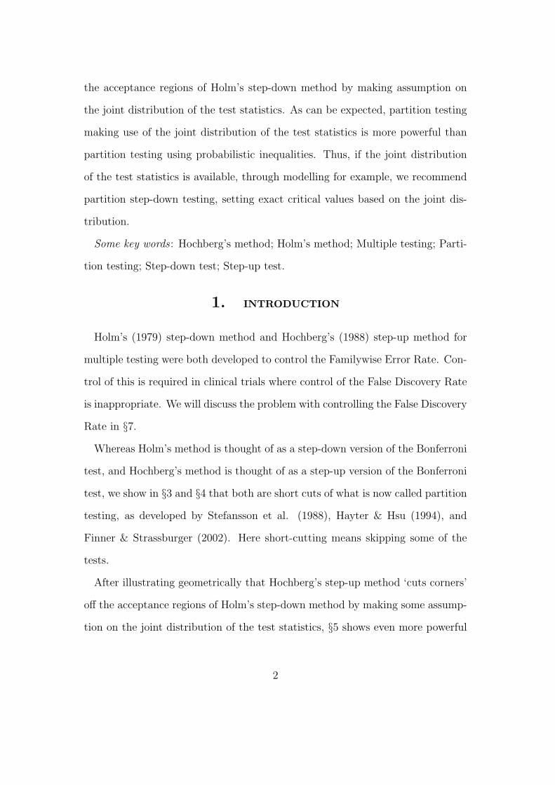
5. GEOMETRY OF HOCHBERG’S STEP-UP METHOD
Using k = 2 as an example, we will show geometrically Hochberg’s step-up
method ‘cuts corner’ off Holm’s step-down method.
Fig. 1 (c) and (d) show the common rejection regions of partition testing for
H∗01 and H∗
02, based on the Bonferroni test and the Simes-Hochberg test. Fig. 1
(a) shows the rejection regions of partition testing H∗012 based on the Bonferroni
test, while Fig. 1 (b) shows the rejection regions of partition testing H∗012 based
on the Simes-Hochberg test.
To see how a short cut is feasible for partition testing based on the Bonferroni
test, take p1 < p2 for example; that is, look at the rejection regions above the
45-degree line in Fig. 1 (a), (c) and (d). If the sample p-values fall inside the
rejection region in Fig. 1 (a), then we know for certain that they will fall inside
the rejection region in Fig. 1 (c) because the rejection region for H∗01 contains
those for H∗012. The test for H∗
01 can therefore be skipped if H∗012 is rejected,
and only H∗02 needs to be tested next. Therefore, the number of tests reduces
from 2k − 1 = 3 to k = 2. The resulted stepwise short cut is Holm’s step-down
method, with rejection regions shown in Fig. 2 (a).
Similarly, to see how a short cut is feasible for partition testing based on the
Simes-Hochberg test, suppose p1 < p2 and look at Fig. 1 (b), (c) and (d). Not
only is the rejection region in Fig. 1 (b) contained by that in Fig. 1 (c) but also
part of it, the triangle defined by (0, 0), (0, α) and (α, α), is the intersection of
the rejection regions in Fig. 1 (c) and (d). This is because the Simes-Hochberg
10

tests in partition testing satisfy the Conditions 1′ − 3′ in which a common set
of the critical values are used. Consequently, the rejection region in Fig. 1 (b)
can be partitioned into two parts, the triangle defined by (0, 0), (0, α) and (α, α)
and the rectangle defined by (0, α), (0, 1), (α/2, 1) and (α/2, α). If the sample
p-values fall inside the triangle, then we know for certain that they will fall inside
the rejection regions in both Fig. 1 (c) and (d). The tests for both H∗01 and
H∗02 can therefore be skipped, and both H01 and H02 can be rejected. If the
sample p-values fall inside the rectangle, then we know for certain that they will
fall inside the rejection regions in Fig. 1 (c) but outside the rejection region in
Fig. 1 (d), so the tests for both H∗01 and H∗
02 can be skipped, and only H01
can be rejected. Therefore, the number of tests reduces from 2k−1 = 3 to k = 2.
The resulting stepwise short cut is Hochberg’s step-up method, with rejection
regions shown in Fig. 2 (b).
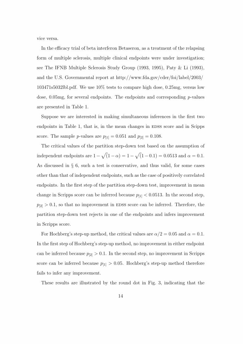
Comparing Fig. 2 (a) and (b), we see that the difference between Holm’s and
Hochberg’s methods lies in the corner of the square defined by (0, 0), (0, α),
(α, 0) and (α, α). That is, Hochberg’s step-up method ‘cuts a corner’ off Holm’s
step-down method.
6. COMPARING STEP-UP TESTS WITH STEP-DOWN TESTS
Since the Simes-Hochberg test cuts corners off the acceptance region of the Bon-
ferroni test, Hochberg’s step-up method is uniformly more powerful than Holm’s
step-down method. This phenomenon seems to have given rise to a misconception
that step-up methods are more powerful than step-down methods. We will show,
instead, that it is easy to construct a step-down method which is not dominated
by Hochberg’s step-up method, and which can also be easily shown to be con-
11

servative for a wider class of test statistics distributions than Hochberg’s step-up
method.
Consider partition testing rejecting H∗0I when p[1]I < 1− (1−α)
1|I| . In essence,
this is a minimum p-value, or maximum statistic, test which computes its critical
values assuming the test statistics are independent. These tests satisfy Conditions
1− 3, so a step-down short cut, which we call the independence step-down test,
proceeds as follows.
Step 1. If p[1] < 1− (1− α)1k , reject H0[1] and go to Step 2; otherwise stop.
Step 2. If p[2] < 1− (1− α)1
k−1 , reject H0[2] and go to Step 3; otherwise stop.
· · ·Step k. If p[k] < α, reject H0[k] and stop.
Since 1− (1−α)1|I| > α/|I|, the independence step-down test is more powerful
than Holm’s step-down method. Figure 3 compares the rejection regions of H∗01,2
for the independence step-down test and Hochberg’s method. The horizontal line
shaded areas are the rejection regions of the independence step-down test, and the
vertical-line shaded areas are the rejection regions of Hochberg’s step-up method.
Clearly, neither dominates the other.
We can compare the strength of condition required for conservatism of the in-
dependence step-down test with that of Hochberg’s step-up test. For brevity, we
indicate this in the setting of one-sided tests with a multivariate normal distribu-
tion. By Slepian’s inequality, see Corollary A.3.1 of Hsu (1996), the independence
step-down test is conservative if the test statistics are nonnegatively correlated.
However, the requirement that their joint distribution has the multivariate to-
tal positivity of order two property is considerably stronger. A necessary and
sufficient condition for multivariate total positivity of order two is that the off-
diagonal elements of the inverse of the variance-covariance matrix all be nonpos-
12

itive. Consider the factor decomposition of the variance-covariance matrix Σ as
Ω+λ1λ′1 + · · ·+λmλ′m, where Ω is a diagonal matrix and the λi’s are column vec-
tors. It is easy to give examples of Σ with covariances all positive whose inverses
have positive off-diagonal elements, even for m = 2. If, however, m = 1 and all
the elements of λ1 are nonnegative, then the joint distribution of the test statis-
tics indeed has the multivariate total positivity of order two property; see Fact
1.3 of Karlin & Rinott (1981) and Theorem 8.3.3 of Graybill (1983). However, for
such a joint distribution, exact critical values of maximum test statistics for H∗0I
can be readily computed numerically, resulting in even more powerful step-down
tests.
Suppose that the test statistics are equally correlated and normally distributed
with correlations equal to 0.5 and variances equal to 1. An example of such a
scenario is multiple comparisons with a control in a clinical trial with a balanced
one-way design. Suppose that k = 3 and α = 0.05. The partitioning step-down
test taking the correlations among the test statistics into account is the step-
down version of Dunnett’s method in this case (Hsu, 1996, Ch. 3) and it has
critical values of 2.062, 1.916 and 1.645. In contrast, the critical values are 2.128,
1.960 and 1.645 for Hochberg’s step-up method and Holm’s step-down method.
There are also stepwise methods that use resampling techniques to take the joint
distribution of the test statistics into account; see for example van der Laan et
al. (2004).
7. A REAL DATA EXAMPLE
The following real data example shows that there are situations in which the
partition step-down test rejects while Hochberg’s step-up method does not, and
13
vice versa.
In the efficacy trial of beta interferon Betaseron, as a treatment of the relapsing
form of multiple sclerosis, multiple clinical endpoints were under investigation;
see The IFNB Multiple Sclerosis Study Group (1993, 1995), Paty & Li (1993),
and the U.S. Governmental report at http://www.fda.gov/cder/foi/label/2003/
103471s5032lbl.pdf. We use 10% tests to compare high dose, 0.25mg, versus low
dose, 0.05mg, for several endpoints. The endpoints and corresponding p-values
are presented in Table 1.
Suppose we are interested in making simultaneous inferences in the first two
endpoints in Table 1, that is, in the mean changes in edss score and in Scipps
score. The sample p-values are p[1] = 0.051 and p[2] = 0.108.
The critical values of the partition step-down test based on the assumption of
independent endpoints are 1−√
(1−α) = 1−√
(1− 0.1) = 0.0513 and α = 0.1.
As discussed in § 6, such a test is conservative, and thus valid, for some cases
other than that of independent endpoints, such as the case of positively correlated
endpoints. In the first step of the partition step-down test, improvement in mean
change in Scripps score can be inferred because p[1] < 0.0513. In the second step,
p[2] > 0.1, so that no improvement in edss score can be inferred. Therefore, the
partition step-down test rejects in one of the endpoints and infers improvement
in Scripps score.
For Hochberg’s step-up method, the critical values are α/2 = 0.05 and α = 0.1.
In the first step of Hochberg’s step-up method, no improvement in either endpoint
can be inferred because p[2] > 0.1. In the second step, no improvement in Scripps
score can be inferred because p[1] > 0.05. Hochberg’s step-up method therefore
fails to infer any improvement.
These results are illustrated by the round dot in Fig. 3, indicating that the
14
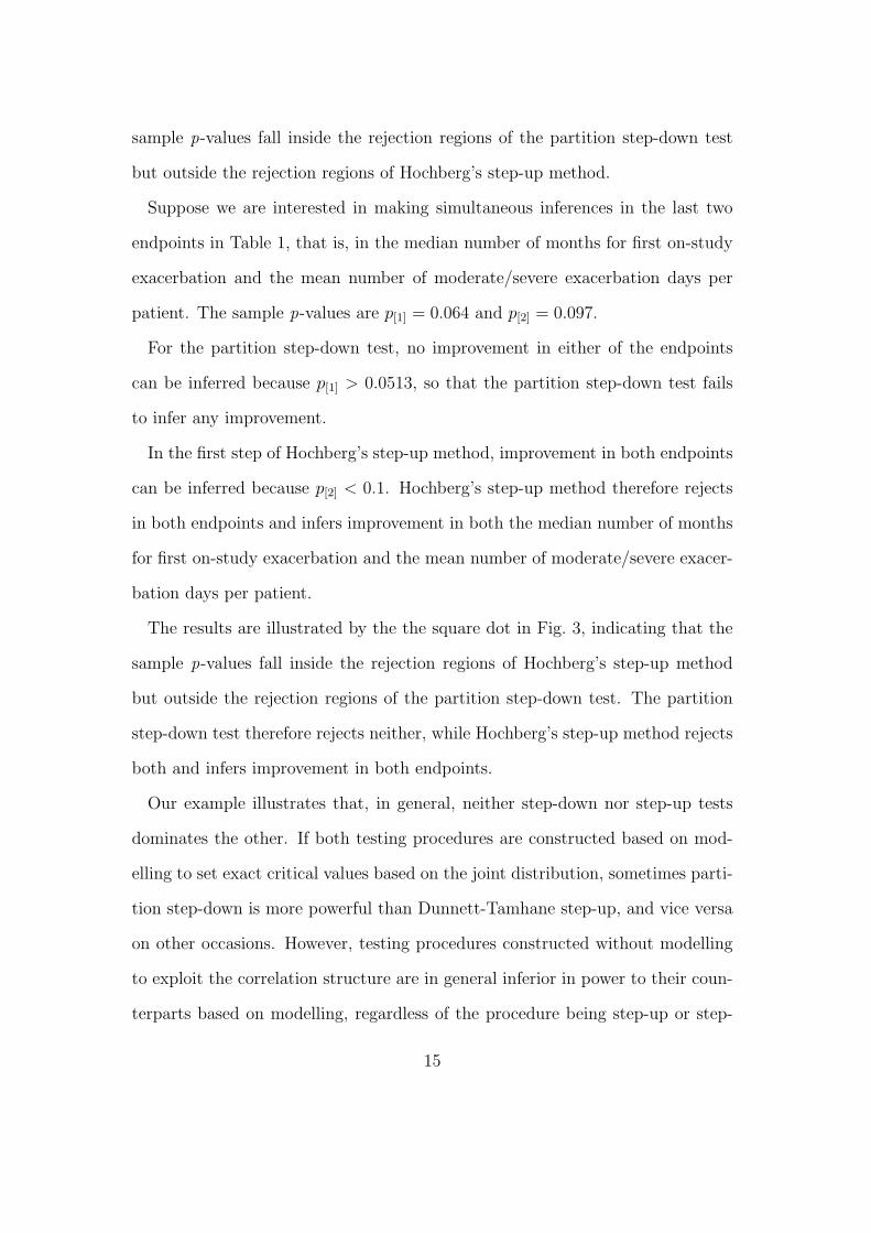
sample p-values fall inside the rejection regions of the partition step-down test
but outside the rejection regions of Hochberg’s step-up method.
Suppose we are interested in making simultaneous inferences in the last two
endpoints in Table 1, that is, in the median number of months for first on-study
exacerbation and the mean number of moderate/severe exacerbation days per
patient. The sample p-values are p[1] = 0.064 and p[2] = 0.097.
For the partition step-down test, no improvement in either of the endpoints
can be inferred because p[1] > 0.0513, so that the partition step-down test fails
to infer any improvement.
In the first step of Hochberg’s step-up method, improvement in both endpoints
can be inferred because p[2] < 0.1. Hochberg’s step-up method therefore rejects
in both endpoints and infers improvement in both the median number of months
for first on-study exacerbation and the mean number of moderate/severe exacer-
bation days per patient.
The results are illustrated by the the square dot in Fig. 3, indicating that the
sample p-values fall inside the rejection regions of Hochberg’s step-up method
but outside the rejection regions of the partition step-down test. The partition
step-down test therefore rejects neither, while Hochberg’s step-up method rejects
both and infers improvement in both endpoints.
Our example illustrates that, in general, neither step-down nor step-up tests
dominates the other. If both testing procedures are constructed based on mod-
elling to set exact critical values based on the joint distribution, sometimes parti-
tion step-down is more powerful than Dunnett-Tamhane step-up, and vice versa
on other occasions. However, testing procedures constructed without modelling
to exploit the correlation structure are in general inferior in power to their coun-
terparts based on modelling, regardless of the procedure being step-up or step-
15

down.
Finally, we discuss why controlling False Discovery Rate is inappropriate in
clinical trials. Suppose there are m + 1 endpoints in a trial and the efficacy
in all of them is required to be demonstrated. If a set of m of the endpoints is
highly efficacious, such as H01, . . . , H0m among H01,. . . , H0m+1 each having the
probability of rejection close to 1, then H0m+1 can be tested with a Type I error
rate higher than α while False Discovery Rate is still controlled at α. This can be
seen in the parameter configuration H0m+1 is true; H01, . . . , H0m are false, and
so false that they will almost surely be rejected. A testing procedure controlling
False Discovery Rate at α has
α = 0 +1
m + 1prm+1 rejections ' 1
m + 1prrejecting H0m+1.
Here H0m+1 is tested at (m + 1)α. Finner & Roters (2001) provides detailed
examples.
ACKNOWLEDGEMENT
Jason Hsu’s research is supported by Grant No. DMS-0505519 from the U.S.
National Science Foundation.
References
Finner, H. & Roters, M. (2001). On the False Discovery Rate and expected Type
I errors. Biomet. J. 43, 985-1005.
Finner, H. & Strassburger, K. (2002). The partitioning principle: a powerful tool
in multiple decision theory. Ann. Statist. 30, 1194-213.
16

Graybill, F. A. (1983). Matrices with Applications in Statistics, 2nd ed. Belmont,
CA: Wadsworth.
Hayter, A. J. & Hsu, J. C. (1994). On the relationship between stepwise decision
procedures and confidence sets. J. Am. Statist. Assoc. 89, 128-36.
Hochberg, Y. (1988). A sharper Bonferroni procedure for multiple tests of signif-
icance. Biometrika 75, 800-2.
Holm, S. (1979). A simple sequentially rejective multiple test procedure. Scand.
J. Statist. 6, 65-70.
Hommel, G. (1988). A stagewise rejective multiple test procedure based on a
modified Bonferroni test. Biometrika 75, 383-6.
Hsu, J. C. (1996). Multiple Comparisons: Theory and Methods. London: Chap-
man and Hall.
Karlin, S. & Rinott, Y. (1981). Total positivity properties of absolute value
multinormal variables with applications to confidence interval estimation
and related probabilistic inequalities. Ann. Statist. 9, 1035-49.
Paty, D. & Li, D. (1993). Interferon beta-1b is effective in relapsing-remitting
multiple sclerosis. II. MRI analysis results of a multicenter, randomized,
double-blind, placebo-controlled trial. Neurology 43, 662-6.
Sarkar, S. (1998). Some probability inequalities for ordered MTP2 random vari-
ables: A proof of the Simes conjecture. Ann. Statist. 26, 494-504.
Simes, R. J. (1986). An improved Bonferroni procedure for multiple tests of
significance. Biometrika 73, 751-4.
Stefansson, G., Kim, W. & Hsu, J. C. (1988). On confidence sets in multiple
comparisons. In Statistical Decision Theory and Related Topics IV, volume
17

2, Ed. S. S. Gupta and J. O. Berger, pp. 89-104. New York: Springer
Verlag.
The IFNB Multiple Sclerosis Study Group, University of British Columbia MS/MRI
Analysis Group (1993). Interferon beta-1b is effective in relapsing-remitting
multiple sclerosis. I. Clinical results of a multicenter, randomized, double-
blind, placebo-controlled trial. Neurology 43, 655-61.
The IFNB Multiple Sclerosis Study Group, University of British Columbia MS/MRI
Analysis Group (1995). Interferon beta-1b in the treatment of multiple scle-
rosis: Final outcome of the randomized, controlled trial. Neurology 45,
1277-85.
van der Laan, M. J., Dudoit, S. & Pollard, K. S. (2004). Multiple testing. part ii.
step-down procedures for control of the family-wise error rate. Statist. Ap-
plic. Genet. Molec. Biol. 3, http://www.bepress.com/sagmb/vol3/iss1/art14.
18

Table 1. Selected results of efficacy trial of Betaseron
Endpoint p-value
Mean change in edss score 0.108
Mean change in Scripps score 0.051
Median number of months for first on-study exacerbation 0.097
Mean number of moderate/severe exacerbation days per patient 0.064
edss, Expanded Disability Status Scale;
Scripps, Scripps Neurologic Rating Score.
19

(a)
p1
p2
α 2
α 2
α
α
0
(b)
p1
p2
α 2
α 2
α
α
0
(c)
p1
p2
α 2
α 2
α
α
0
(d)
p1
p2
α 2
α 2
α
α
0
Figure 1: Rejection regions of partition testing with k = 2. (a) Rejection regionof the Bonferroni test for H∗
012. (b) Rejection region of the Simes-Hochberg test
for H∗012. (c) Rejection region of the Bonferroni test and the Simes-Hochberg
test for H∗01. (d) Rejection region of the Bonferroni test and the Simes-Hochberg
test for H∗02.
20

(a)
p1
p2
α 2
α 2
α
α
0
A
B
c
(b)
p1
p2
α 2
α 2
α
α
0
D
E
F
Figure 2: Rejection regions of Holm’s and Hochberg’s methods. (a) Rejectionregions of Holm’s step-down method. In region A both H01 and H02 are rejected.Rectangle B is the region where only H01 is rejected. Rectangle C is the regionwhere only H02 is rejected. (b) Rejection regions of Hochberg’s step-up method.Square D is the region where both H01 and H02 are rejected. Rectangle E is theregion where only H01 is rejected. Rectangle F is the region where only H02 isrejected.
21

p1
p2
1 − (1−α)=0.0513
1 − (1−α)=0.0513
α 2=0.05
α 2=0.05
α=0.1
α=0.1
0
Figure 3: Comparison of Hochberg’s step-up method and the independence step-down test. The horizontal lines indicate the rejection regions of the independencestep-down test. The vertical lines indicate the rejection regions of Hochberg’sstep-up method. The round dot represents the sample p-values of (0.108, 0.051).The square dot represents the sample p-values of (0.097, 0.064). The distancebetween α/2 = 0.05 and 1−
√(1−α) = 0.0513 in this figure has been artificially
expanded in scale for the sake of graphical clarity.
22