HISTORY AND VALUE OF UNCERTAINTY AND SENSITIVITY ANALYSES AT THE NUCLEAR

REGULATORY COMMISSION AND CENTER FOR NUCLEAR WASTE REGULATORY ANALYSES

Prepared for

U.S. Nuclear Regulatory Commission Contract NRC–02–07–006

Prepared by

Sitakanta Mohanty1 Richard Codell2

Y.-T. (Justin) Wu2 Osvaldo Pensado1 Olufemi Osidele1

David Esh3 Tina Ghosh3

1Center for Nuclear Waste Regulatory Analyses 2Consultant

3U.S. Nuclear Regulatory Commission

September 2011

ii

ABSTRACT

This report documents the uncertainty and sensitivity analysis knowledge acquired over the past 20 years by the U.S. Nuclear Regulatory Commission (NRC) and the Center for Nuclear Waste Regulatory Analyses (CNWRA®) staffs during preparations to develop site-specific regulations for disposal of high-level radioactive waste (HLW) at the proposed Yucca Mountain repository, and to review a license application for that repository. This report is intended to serve the needs of future performance assessors or risk analysts at NRC and CNWRA who may be engaged in future HLW-related regulatory activities. It is intended to serve as a starting point for understanding various uncertainty and sensitivity analysis methods used by the two staffs, several of which were developed in house. Through references, this report points to various other documents for details of the uncertainty and sensitivity analyses staffs produced. For completeness, a chapter in this report also summarizes early uncertainty and sensitivity analyses work for waste package performance assessment (PA) that was carried out during the late 1980s. Uncertainty and sensitivity analysis methods the two staffs developed evolved and matured over time. In some cases, more advanced techniques were developed, and in others, existing advanced methods were used to glean risk insights from PAs. The generality of methods presented in this report also make them applicable to other NRC nuclear fuel cycle programs.

iii

CONTENTS Section Page

ABSTRACT ................................................................................................................................... ii FIGURES ..................................................................................................................................... vi TABLES ...................................................................................................................................... viii EXECUTIVE SUMMARY ............................................................................................................. ix ACKNOWLEDGMENTS ............................................................................................................. xiii

1 INTRODUCTION ............................................................................................................ 1-1

1.1 Objectives of the Report .................................................................................. 1-3 1.2 A Brief Description of the Performance Assessment Models .......................... 1-3

1.2.1 System Conceptualization and Model Description ........................... 1-4 1.2.2 System Performance Estimation ...................................................... 1-4 1.2.3 Performance Metrics ......................................................................... 1-7

1.3 Report Structure .............................................................................................. 1-7 2 UNCERTAINTY ANALYSIS ........................................................................................... 2-1

2.1 Introduction ...................................................................................................... 2-1 2.2 Risk, and Risk Assessment ............................................................................. 2-1

2.2.1 Repository Risk Assessment ............................................................ 2-2 2.2.2 Uncertainty in the Context of Performance Assessment .................. 2-3 2.2.3 Parameter Sampling ......................................................................... 2-4 2.2.3.1 Distribution Functions for Parameters ............................. 2-4 2.2.3.2 Developing Empirical Probability Density Functions ....... 2-4 2.2.3.3 The Maximum Entropy Formalism .................................. 2-6 2.2.3.4 Sampling From a Distribution Function ........................... 2-7 2.2.4 Parameter Correlations ..................................................................... 2-7 2.2.5 Convergence of Model Results ......................................................... 2-9 2.2.6 Calculation of the Peak-of-the-Mean Dose ....................................... 2-9 2.2.7 Calculation of Mean Dose for Disruptive Events ............................ 2-10 2.2.8 Risk Dilution .................................................................................... 2-13

2.3 Granularity and Upscaling of Performance Assessment Models .................. 2-13 2.3.1 Example .......................................................................................... 2-14 2.3.2 Conclusions on Uncertainty Analysis .............................................. 2-16

3 SENSITIVITY ANALYSIS ............................................................................................... 3-1

3.1 General Considerations in Sensitivity Analysis ............................................... 3-1 3.1.1 Sensitivity to Alternative Models ....................................................... 3-1 3.1.2 Use of Intermediate Results To Determine Model Importance ......... 3-1 3.1.3 Use of Barrier or Component Failure Analysis ................................. 3-1 3.1.4 Parameter Sensitivity Analysis ......................................................... 3-2

3.2 Traditional Techniques for Parameter Sensitivity ............................................ 3-2 3.2.1 Statistical Sensitivity Analysis Based on Monte Carlo Sampling ...... 3-2 3.2.1.1 Developing and Manipulating Model Results for Sensitivity Analysis .......................................................... 3-3 3.2.1.2 Variable Transformations and Their Attributes ................ 3-3 3.2.2 Regression Methods ......................................................................... 3-6 3.2.2.1 Single Linear Regression on One Variable ..................... 3-6 3.2.2.2 Stepwise Multiple Linear Regression .............................. 3-7 3.2.2.3 Sensitivity for Non-Monotonic Relationships ................... 3-8

iv

CONTENTS (continued) Section Page

3.2.3 Nonparametric Methods ................................................................... 3-9 3.2.3.1 The Kolmogorov-Smirnov Test ....................................... 3-9 3.2.3.2 The Sign Test ................................................................ 3-10 3.2.3.3 The Wilcoxon Rank Sum Test ....................................... 3-11

3.3 Conclusions ................................................................................................... 3-12 4 ADVANCED AND SPECIAL-CASE SENSITIVITY TECHNIQUES ................................ 4-1

4.1 Introduction ...................................................................................................... 4-1 4.2 Cumulative Distribution Function Sensitivity Analysis Method ........................ 4-1

4.2.1 Sampling-Based Cumulative Distribution Function Sensitivities ....... 4-2 4.2.2 Confidence Limits for Accepting Insignificant Parameters ................ 4-4 4.2.3 TPA Examples .................................................................................. 4-4 4.2.4 Correlation Issues ............................................................................. 4-6 4.2.5 Sample Size Requirements .............................................................. 4-7 4.2.6 Summary .......................................................................................... 4-7

4.3 Genetic Algorithms With Cascaded Variable Selection ................................... 4-8 4.3.1 Example—Shallow Land Disposal of Saltstone ................................ 4-8 4.3.2 Conclusions ...................................................................................... 4-9

4.4 Regionalized Sensitivity Analysis .................................................................. 4-10 4.4.1 The Regionalized Sensitivity Analysis Procedure ........................... 4-10 4.4.2 Example .......................................................................................... 4-12 4.4.3 Discussion ...................................................................................... 4-13 4.4.4 Summary ........................................................................................ 4-14

4.5 Fractional Factorial Method ........................................................................... 4-16 4.6 Iterated Fractional Factorial Design ............................................................... 4-18 4.7 Parameter Tree and Distribution Partitioning Intercept Methods ................... 4-18

4.7.1 Parameter Tree Method .................................................................. 4-18 4.7.1.1 Parameter Tree Example .............................................. 4-21 4.7.2 Distribution Partitioning Intercept Method ....................................... 4-22 4.7.2.1 Distribution Partitioning Intercept Example ................... 4-23 4.7.3 Discussion ...................................................................................... 4-23

4.8 Barrier Performance Evaluation by Signal Processing Techniques .............. 4-26 4.8.1 Convolution and Deconvolution Using the Fourier Transform ........ 4-27 4.8.1.1 Example—Deconvolution of Pu-242 Results ................ 4-27 4.8.2 Conclusions .................................................................................... 4-30

4.9 Component Sensitivity Analysis .................................................................... 4-30 4.10 Strategic Partitioning of Assumption Ranges and Consequences Methodology ......................................................................... 4-31

4.10.1 Steps in Strategic Partitioning of Assumption Ranges and Consequences Methodology ...................................... 4-34 4.10.2 Conclusions .................................................................................... 4-36

4.11 Distributional Sensitivity Analysis .................................................................. 4-37 5 INTERPRETING SENSITIVITY RESULTS .................................................................... 5-1

5.1 Introduction ...................................................................................................... 5-1 5.2 Collating Parameter Sensitivity Results From Multiple Methods ..................... 5-1 5.3 Verification of Sensitivity Analysis Results ...................................................... 5-3 5.4 Top-Down Correlations .................................................................................... 5-4

v

CONTENTS (continued) Section Page

5.5 Effect of Using Peak Doses To Calculate Sensitivities .................................... 5-6 5.6 Effect of Model Conservatism on Sensitivity Studies ...................................... 5-6

5.6.1 Approach .......................................................................................... 5-8 5.7 Conclusions ..................................................................................................... 5-9

6 EARLIER ACTIVITIES ON WASTE-PACKAGE PROBABILISTIC

PERFORMANCE ANALYSES ....................................................................................... 6-1 6.1 Introduction ...................................................................................................... 6-1

6.1.1. Background ....................................................................................... 6-1 6.2 Waste Package Performance Assessment ..................................................... 6-2

6.2.1 Introduction ....................................................................................... 6-2 6.2.2 Waste Package Failure Modes and Uncertainties ............................ 6-3 6.2.3 Probabilistic Performance Assessment and Probabilistic Modeling ...................................................................................... 6-4

6.3 Uncertainty Evaluation Methods ...................................................................... 6-4 6.3.1 Introduction ....................................................................................... 6-4 6.3.2 Probability Distribution Approach ...................................................... 6-6 6.3.2.1 Simplifying Performance Functions ................................. 6-6 6.3.2.2 Fast Probabilistic Analysis Methods ................................ 6-6 6.3.3 Bounding Approach .......................................................................... 6-8 6.3.4 Expert Judgment ............................................................................... 6-9 6.3.5 Sensitivity Analysis ........................................................................... 6-9

6.4 Fast Probabilistic Performance Assessment Example .................................. 6-10 6.5 Summary ....................................................................................................... 6-11

7 SUMMARY ..................................................................................................................... 7-1

7.1 Uncertainty Analysis ........................................................................................ 7-2 7.2 Sensitivity Analyses ......................................................................................... 7-3 7.3 Model Conservatism Study .............................................................................. 7-5 7.4 Earlier Activities Related to Waste Package ................................................... 7-5 7.5 Conclusions ..................................................................................................... 7-6

8 REFERENCES ............................................................................................................... 8-1 APPENDIX A — A COLLECTION OF SOME ALGORITHMS USED FOR

SENSITIVITY/UNCERTAINTY ANALYSES IN NRC WASTE MANAGEMENT PROGRAMS

vi

FIGURES Figure Page 1-1 Processes in NRC’s TPA Version 5.1 Performance Assessment Code ..................... 1-5 2-1 Monte Carlo Modeling of Repository Performance ..................................................... 2-2 2-2 Random Sampling from a Single Distribution Function ............................................... 2-7 2-3 Latin Hypercube Sampling for Two Variables ............................................................. 2-8 2-4 Parameter Correlation Example .................................................................................. 2-8 2-5 Calculation of Peak-of-the-Mean Dose for Three Realizations ................................. 2-10 2-6 Mean Conditional Dose Curves for ASHPLUME With Different Event Times ........... 2-11 2-7 Convergence of Mean Dose Curve Using Convolution and Regular Averaging of Realizations, ASHPLUME, and TEPHRA Extrusive Volcanism Models ................... 2-12 2-8 Two Distributions for Drip Shield Failure Time .......................................................... 2-13 2-9 Dissolve Radionuclide Release Model for Iterative Performance Assessment ......... 2-14 3-1 Mapping a Distribution Into a Standard Normal Distribution ....................................... 3-5 3-2 Effect of Stepwise Regression of Peak Dose on Residual Sum of Squares ............... 3-8 3-3 Kolmogorov-Smirnov Test ......................................................................................... 3-10 4-1 Sampling-Based Cumulative Distribution Function Sensitivity Analysis Method .......................................................................................................... 4-2 4-2 Examples of Acceptance Limits .................................................................................. 4-5 4-3 Cumulative Distribution Function Sensitivities Sμ for Top 10 Parameters Having

Highest Average .......................................................................................................... 4-5 4-4 Cumulative Distribution Function Sensitivities Sσ for Top 10 Parameters Having Highest Average .......................................................................................................... 4-6 4-5 Performance Standard Deviation Before and After Fixing 1, 2, 3, 4, and 10 Most Influential Variables at Mean Values ........................................................................... 4-7 4-6 Illustration of Binary Classification of Model Results (у) Showing an Acceptable Realization (Below Threshold) and an Unacceptable Realization (Above Threshold) ..................................................................................................... 4-11 4-7 Illustration of the Parameter Space for a Hypothetical Two-Dimensional Model Showing the Classification of the Parameters ................................................ 4-11 4-8 Illustration of the Two-Sample Kolmogorov-Smirnov Test for a Two-Parameter Model. dm,n Is the Maximum Vertical Distance ......................................................... 4-12 4-9 Dose Curves From 500 Random Realizations of the TPA Code .............................. 4-13 4-10 Tree diagram From Factorial Design Results for 100,000-Year Simulation Period, TPA Version 4.1 ........................................................................................................ 4-17 4-11 Scatter Plot, Output y Versus Input x, and Subset Split for the Computation of the Parameter Tree Statistic............................................................................................ 4-19 4-12 Comparison of Analytical Cumulative Distribution Function in Eq. (4-20) to a Numerical Distribution Computed by Using Eq. (4-17), Random Sampling .............. 4-20 4-13 Example of an Application of the Parameter Tree Sensitivity Index, Ipt, To Analyze the Output of a Stochastic Performance Assessment Model .................................... 4-21 4-14 (a) Scatter Plot, Output y Versus Input x, and Identification of the Outstanding Set; (b) Computation of the p-Intercept Statistic as the Probability Intercept ................... 4-23 4-15 Example of an Application of the Distribution Partitioning Intercept Sensitivity Index, Idpi, to Analyze the Output of a Stochastic Performance Assessment Model ............ 4-24

vii

FIGURES (continued) Figure Page 4-16 Identification of Influential Parameters to the Output Using a Technique Based on Correlation Coefficients ............................................................................................. 4-25 4-17 Transfer Function for Pu-242 in Unsaturated Zone ................................................... 4-29 4-18 Applying Transfer Function (i.e., Factor of 0.6615) to Engineered Barrier System Releases To Reproduce Unsaturated Zone Release ................................................ 4-29 4-19 Transfer Function for Release of Pu-242 in Saturated Zone Results for Tc-99 ........ 4-30 4-20 Exhaustive Combinations of Component Sensitivity Analysis Cases for Six Components in the Example Problem ....................................................................... 4-32 4-21 A Scenario Defined as a Collection of Intervals of Performance Assessment Parameter Distributions ............................................................................................. 4-34 4-22 Cumulative Distribution Functions for Substantially Increased Doses and Nonsubstantially Increased Dose Realizations for Parameter WPFlowMF ............... 4-35 4-23 Substantially Increased Doses (●) Versus Nonsubstantially Increased Doses (▲) in Space of Sampled Values of Parameters AAMAI@s and SAW% ......................... 4-36 4-24 Strategic Partitioning of Assumption Ranges and Consequences Tree for Class of Scenarios With Influential Parameters in the Worst 5 Percent Intervals ................... 4-37 4-25 Example of (a) Changing the Probability Density Function for an Input Parameter by Shifting the Mean Value of a Normal Distribution Function .................................. 4-38 5-1 Effect on Complementary Cumulative Distribution Function of Peak Doses of Identified Influential Parameters .................................................................................. 5-4 5-2 Sensitivity Using Doses for Each Realization at Time of Peak-of-the-Mean Dose ..... 5-7 5-3 Sensitivity Using Peak Doses From Each Realization ................................................ 5-7 6-1 Fast Probability Integration Concept ........................................................................... 6-7 6-2 Advanced Mean Value for Fast Cumulative Distribution Function Analysis ................ 6-8 6-3 A Fast Probabilistic Performance Assessment Computational Framework for Engineered Barrier System .................................................................................. 6-10 6-4 Container Lifetime Cumulative Distribution Function Using Monte Carlo and Fast Probabilistic Performance Assessment Method ................................................ 6-11 6-5 Complementary Cumulative Distribution Function of Radionuclide Release Using Monte Carlo and Advanced Mean Value Method ...................................................... 6-12

viii

TABLES Table Page 2-1 Some Useful Distributions From Maximum Entropy Formalism .................................. 2-6 4-1 Rankings of Influential Parameters Conditioned on 10th-, 50th-, 75th-, and 90th-Percentile Dose Thresholds ............................................................................... 4-14 4-2 Schematics of Scatter Plot Kinds, and Qualitative Discussion on Whether the Correlation, Parameter Tree, and Distribution Partitioning Intercept Techniques Can Identify Relationships Between x and y ............................................................. 4-15 5-1 Ranks of 10 Most Significant Variables for 10,000 Years From First 6 Statistical Tests ........................................................................................................ 5-2 5-2 Influential Parameters for the 10,000-Year Simulation Period From Sensitivity Analysis Studies .......................................................................................................... 5-3 5-3 Changes in Variance for Holding Identified Influential Parameters at Their Mean Values Individually ...................................................................................................... 5-5 6-1 Uncertainty Evaluation Methods .................................................................................. 6-5

ix

EXECUTIVE SUMMARY

The U.S. Nuclear Regulatory Commission (NRC), with assistance from the Center for Nuclear Waste Regulatory Analyses (CNWRA®), has conducted technical evaluations of U.S. Department of Energy (DOE) analyses to determine whether a proposed repository at Yucca Mountain would be technically defensible and meet all applicable safety requirements. Preceding this review, NRC had numerous prelicensing interactions with DOE over a 20-year period to ensure a complete, high-quality license application (Eisenberg, et al., 1999). The Commission’s probabilistic risk assessment (PRA) policy statement (Federal Register, 1995) has encouraged the use of the PRAs in regulatory requirements and reviews. Performance assessment (PA) is the manifestation of PRA in the context of waste management and is the process for quantitatively evaluating the ability of a disposal facility to contain and isolate radioactive waste (Campbell and Cranwell, 1988). Consistent with this policy, the NRC staff, with assistance from CNWRA, developed and used PAs to facilitate interactions with DOE and conduct various reviews along the way. Evaluation of uncertainties and prioritization of features, events, and processes important to safety through sensitivity analysis (also referred to as uncertainty importance analysis) are important aspects of any PA. Uncertainty analysis attempts to quantify the uncertainty in performance estimates. Sensitivity analysis attempts to evaluate the fractional change in the performance estimates in response to alternative models or changes to the parameters of those models. This report summarizes the uncertainty and sensitivity analysis activities at NRC and CNWRA in the NRC program area of high-level radioactive waste (HLW) repository safety. The report also provides a brief background on the performance assessment activities to provide the context for the uncertainty and sensitivity analysis activities. NRC has carried out uncertainty and sensitivity analysis activities since the 1980s for performance assessments in NRC’s HLW program. NRC has pursued performance assessment methodology development for a variety of geologic media including bedded salt, basalt, and tuff (Bonano, et al., 1989; Gallegos, 1991; Eisenberg, 1999). Starting in the late 1980s, NRC staff developed independent performance assessment capabilities through a series of Iterative Performance Assessment (IPA) phases: Phase I (Codell, et al., 1992), completed in 1991; Phase II (Wescott, et al., 1995), completed in 1993; and Phase III (planning), completed in 1995. The process continued with increasing involvement of CNWRA to develop several versions of NRC’s performance assessment code (i.e., TPA Code, Versions 3.1, 3.1.3, 3.1.4, 3.2, 4.1, 5.0, and 5.1). These developments roughly paralleled DOE’s performance assessments such as the Total System Performance Assessment–Viability Assessment (DOE, 1998) and the Total System Performance Assessment–Site Recommendation (CRWMS M&O, 2000). Each phase of uncertainty and sensitivity analyses enabled NRC staff to gradually move from preliminary models to more sophisticated and matured methodologies, and from preliminary to more in-depth risk insights through better understanding of features, events, and processes. Topics discussed in this report include propagating uncertainty in models by the use of random sampling of input parameters, generating the risk basis, the peak-of-the-mean criterion for risk, risk dilution, convergence of the risk curve, and granularity. Systematic examination of uncertainty representation through input parameters is needed for a probabilistic model to be defensible. The probability density functions (PDFs) of input parameters need to be defensible especially because (i) too broad uncertainty ranges may cause risk dilution and (ii) too narrow uncertainty ranges may indicate unwarranted confidence

x

in the parameter range, and therefore bias the results. Bias could affect results from sensitivity analyses. Because input parameters are best understood by the analysts, a questionnaire was developed for all those involved in the performance assessment to aid in the understanding of each other’s needs to develop the PDFs with an appropriate level of technical basis. Methods are available (e.g., maximum entropy formalism) to help develop the best possible PDFs from the available information. Model outputs after uncertainty propagation were used to develop the risk basis by computing expected dose as a function of time from the Monte Carlo results. A special technique was developed to synthesize the risk curve for disruptive events that were of low probability but often had relatively large doses that decayed rapidly. “Upscaling” and “granularity” were studied to determine how the necessary coarse representation of aspects of the repository (e.g., waste packages) could best determine overall behavior. Various traditional and nontraditional sensitivity analysis methods were used to identify influential parameters, models, and components driving performance. Traditional methods included statistical, regression, and nonparametric tests. Statistically based traditional methods took advantage of the large set of model runs generated for uncertainty analyses. The analyses were performed on either the original input set and output value pairs or transformed-value pairs to enhance the sensitivity calculations. Regression methods included linear regression on one variable, stepwise multiple regression, and nonparametric tests. Special techniques were developed and used when the relationships between the parameters and the output were non-monotonic. Nonstatistical sensitivity analysis techniques required sets of model runs with inputs specified by the method. Distributional sensitivity analysis was used to reveal improper choices of PDFs. In general, the various sensitivity methods presented would rank the importance of the parameters in a different order from each other. The staff did not make strong recommendations for one sensitivity technique over another because it was impractical to forecast under what range of conditions any method would be most accurate. Instead, a consensus approach was used to evaluate the results of multiple sensitivity methods to determine the most sensitive parameters according to their rank by each method. The identified sensitive parameters were numerically validated either by (i) removing the most sensitive parameters from sampling to see whether they reduced the uncertainty in the results or (ii) sampling only the most-sensitive parameters while keeping the other parameters fixed to see whether the results are similar to the basecase results. Sensitivity analyses were conducted using both the peak doses from each realization or the doses at the time that the peak-of-the-mean dose curve occurred. In some cases, the two approaches led to a different ranking of the sensitivities, especially for parameters that determined the time that the peak doses occurred. Parameter distributions chosen by the analysts often erred on the side of safety by picking conservative end points for the PDFs. Analyses were conducted to illustrate how conservatism in model parameters can influence the sensitivity based ranking of influential parameters. Results showed that the sensitivity of model output changes nonlinearly with the conservatism built into the model through the assumptions for parameter values.

xi

A number of uncertainty and sensitivity analysis methods were developed and used during the early stage of the repository program (late 1980s). The focus at the time was on waste package performance, and the applicable regulations was 10 CFR Part 60, which has a substantially complete containment requirement. Four uncertainty evaluation methods (probability distribution approach, bounding approach, expert judgment, and sensitivity analysis) were identified as elements of a probability based framework that, without either diminishing or enhancing the input uncertainties, can provide quantitative measures for assessing waste package design performance. Through uncertainty and sensitivity analysis in performance assessment, NRC staff prioritized reviews and determined key areas for interactions with DOE. At a programmatic level, this analysis capability enabled NRC staff to interact more effectively with DOE on the total system performance assessments that DOE developed during the prelicensing activities; to formulate a risk-informed, site-specific standard; and to develop appropriate guidance. It helped NRC and CNWRA staffs to develop experience and insights necessary for effective prelicensing interactions with DOE and to confirm staff understanding about important features, events, and processes that needed further careful assessment. At a technical level, these analyses have helped NRC staff to decide which portions of the DOE assessment required focus through further detailed quantitative analyses to successfully demonstrate compliance with the safety standard. Some of the areas prompted by uncertainty and sensitivity analyses for discussion included modeling assumptions, conceptual models, data needs, revisions to the site characterization program, and decisions on the use of expert judgment versus additional data collection. The methods developed and used and the experience gained are general enough to find broad applications across other NRC activities, such as low-level waste disposal and nuclear fuel cycle-related activities such as storage, transportation, and nuclear power plant safety. References Bonano, E.J., P.A. Davis, L.R. Shipoers, K.F. Brinster, W.E. Beyeler, C.D. Updegraff, E.R. Shepherd, L.M. Tilton, and K.K. Wahi. NUREG/CR–4759, SAND86–2325, “Demonstration of a Performance Assessment Methodology for High-Level Radioactive Waste Disposal in Basalt Formations.” Washington, DC: NRC. June 1989. Campbell, J.E. and R.M. Cranwell. “Performance Assessment of Radioactive Waste Repositories.” Science. Vol. 239, No. 4846. pp. 1,389–1,392. 1988. Codell, R.B, N. Eisenberg, D. Fehringer, W. Ford, T. Margulies, T. McCartin, J. Park, and J. Randall. NUREG–1327, “Initial Demonstration of the NRC’s Capability To Conduct a Performance Assessment for a High-Level Waste Repository.” Washington, DC: NRC. May 1992. CRWMS M&O. “Total System Performance Assessment for Site Recommendation.” TDR–WIS–PA–000001. Rev 00, ICN 01. MOL.20001220.0045. Las Vegas, Nevada: CRWMS M&O. 2000. DOE. DOE/RW–0508, “Total System Performance Assessment. Volume 3 of Viability Assessment of a Repository at Yucca Mountain.” MOL: 19981007.0030. Washington, DC: U.S. Department of Energy, Office of Civilian Radioactive Waste Management. 1998.

xii

Eisenberg, N.A., M.P. Lee, T.J. McCartin, K.I. McConnell, M. Thaggard, and A.C. Campbell. “Development of a Performance Assessment Capability in the Waste Management Programs of the U.S. Nuclear Regulatory Commission.” Risk Analysis. Vol. 19, No. 5. pp. 847–876. 1999. Federal Register. “Use of Probabilistic Risk Assessment Methods in Nuclear Regulatory Activities—Final Policy Statement. Federal Register. Vol. 7, No. 158. pp. 42622–42629. August 1995. Gallegos, D.P. NUREG/CR–5701, “Performance Assessment Methodology for High-Level Radioactive Waste Disposal in Unsaturated, Fractured Tuff.” Washington, DC: NRC. July 1991. Wescott, R.G., M.P. Lee, N.A. Eisenberg, T.J. McCartin, and R.G. Baca, eds. “NUREG–1464, “NRC Iterative Performance Assessment Phase 2.” Washington, DC: NRC. October 1995.

xiii

ACKNOWLEDGMENTS This report describes work performed by the Center for Nuclear Waste Regulatory Analyses (CNWRA) and its contractors for the U.S. Nuclear Regulatory Commission (USNRC) under Contract No. NRC–02–07–006. The activities reported here were performed on behalf of the USNRC Office of Nuclear Material Safety and Safeguards, Division of High Level Waste Repository Safety. This report is an independent product of the CNWRA and does not necessarily reflect the view or regulatory position of the USNRC. The USNRC staff views expressed herein are preliminary and do not constitute a final judgment or determination of the matters addressed or of the acceptability of any licensing action that may be under consideration at USNRC. Dr. Bruce Goodwin (consultant) assisted several years ago in formulating questions to elicit information from performance assessors and process-level subject matter experts. His contribution to this work is gratefully acknowledged. The authors express their appreciation to Mr. Timothy McCartin (NRC) for his valuable comments on this report. The authors also express their appreciation to J. Winterle for his technical review, J. McMurry for her informal review, G. Wittmeyer for his programmatic review, L. Mulverhill for her editorial review, and L. Selvey for her administrative support.

QUALITY OF DATA, ANALYSES, AND CODE DEVELOPMENT DATA: All CNWRA-generated original data contained in this report meet the quality assurance requirements described in the Geosciences and Engineering Division Quality Assurance Manual. Calculations have been recorded in CNWRA Scientific Notebook Number 1083E and 1084E (Codell, 2011a,b). Sources for other data should be consulted for determining the level of quality for those data. ANALYSES AND CODES: R statistical platform (Hornick, 2007) was used for calculations documented in the scientific notebooks. NeuralWorks Predict® (NeuralWare, 2001) was used to regenerate a small fraction of calculations carried out by one of the authors several years ago. REFERENCES Codell, R. Scientific Notebook 1083E. San Antonio, Texas: CNWRA. 2011a. Codell, R. Scientific Notebook 1084E. San Antonio, Texas: CNWRA. 2011b. Hornick, K. “The R FAQ—Frequently Asked Questions on R.” <http://CRAN.R-Project.org/doc/FAQ/> ISBN3–900051–08–9. 2007. NeuralWare. “NeuralWorks Predict® Product Version 2.40.” Carnegie, Pennsylvania: NeuralWare. 2001.

1-1

1 INTRODUCTION

For more than two decades, the U.S. Department of Energy (DOE) characterized site geology, designed engineered barriers, and conducted performance assessment (PA) studies for a potential geologic repository for high-level radioactive waste (HLW) and spent nuclear fuel at Yucca Mountain, Nevada. By statute, the U.S. Nuclear Regulatory Commission (NRC) had the sole responsibility for reviewing any license application DOE submitted to construct a repository. DOE conducted analyses to demonstrate the safety of the repository, included these analyses in a safety analysis report (SAR), and submitted the analyses to NRC in support of its license application. NRC conducted a technical assessment of information presented in the SAR and documented in a technical evaluation report (TER) the technical insights on the application of PA in the context of geologic disposal. DOE’s submittal of the SAR was preceded by nearly 20 years of interactions with NRC, referred to as prelicensing interactions. Because this was a first-of-a-kind facility, NRC–DOE prelicensing interactions were designed to ensure a complete, high-quality license application that NRC would be able to review within the limited statutory period. In the mid-1990s, several years into the prelicensing period, NRC issued a policy statement that advocated using risk-informed, performance-based approaches in developing and implementing regulations, and directed staff to increase its use of probabilistic risk assessment (PRA) in all regulatory activities to the extent supported by the state-of-the-art in methods and data. The Commission envisioned a risk-graded approach where the staff would use risk information to focus on those licensee activities that pose the greatest risk to the public health and safety (NRC, 1997). PRA was emphasized in the context that as a systematic method, it would provide a system-level understanding of the performance of a nuclear system, particularly in terms of providing an understanding of the likely outcomes given uncertainties, sensitivities, areas of importance, interactions among the components and processes, and the capability of individual system components and processes (NRC, 2003; Callan, 1998). PA is the manifestation of PRA in the context of waste management and is the process for quantitatively evaluating the ability of a disposal facility to contain and isolate radioactive waste (Campbell and Cranwell, 1988). NRC’s HLW Repository Safety program undertook a Risk Insights Initiative to risk inform prelicensing regulatory activities and license application review activities The intent was that by having risk insights information, staff could develop a perspective that would enable them to review more readily the information DOE provided for NRC to make determinations based on information available at the time. There was an additional desire to train staff to conduct risk-informed, performance-based issue resolutions and reviews so they would specifically look for, among other things,1 explicit identification and quantification of sources of uncertainty in the analysis and test the sensitivity of the results to key assumptions and uncertainties. Staff not only planned to draw risk insights from the review of DOE’s analyses and extensive technical interactions with DOE and other groups, but also from experience gained through independent PAs. Consequently, independent PAs became a major component of risk insights development activities. Independent PAs included quantitative analyses of system-level performance (e.g., analyses using NRC’s system-level code or simplified models that result in a calculation of probability weighted dose) as well as supporting analyses (e.g., calculation of waste package failure rates, release rates of radionuclides from the waste package, and 1Explicit consideration of potential challenges to safety; logical means for prioritizing these challenges, based on risk significance, engineering judgment, and/or other considerations.

1-2

transport times of radionuclides to the compliance location) that helped understand the system-level results. PA was not new to NRC nor was the Commission’s policy statement of the 1990s the start of PAs. In fact, NRC’s HLW program had carried out PAs since the early 1970s, including uncertainty and sensitivity analysis activities. Sandia National Laboratories developed a PA methodology for NRC to evaluate HLW disposal in a hypothetical repository, initially in bedded salt formations and later in basalt and tuff (Bonano, et al., 1989a; Gallegos, 1991; Eisenberg, 1999). Starting in the late 1980s, NRC staff developed independent PA capabilities through a series of Iterative Performance Assessment (IPA) phases. Phase I (Codell, et al., 1992) was completed in 1991 and Phase II (Wescott, et al., 1995) was completed in 1993. Performance measures at this time were consistent with regulations in 40 CFR Part 191 (U.S. Environmental Protection Agency, 1993) and 10 CFR Part 60 (Code of Federal Regulations, 1991), which had subsystem requirements. The Center for Nuclear Waste Regulatory Analyses (CNWRA®) participation in PA activities began with Phase II activities. NRC planned for Phase III in 1995 to refocus the prelicensing repository program on Key Technical Issues (KTIs)—topics most critical to repository performance based on the review of DOE’s site characterization program and DOE’s TSPA code. NRC and CNWRA staffs used PA methods coupled with the KTI-based program to develop guidance on methods to evaluate the significance of technical uncertainties and reduce uncertainties to the extent practical, before submitting the license application. Over the next several years, uncertainty and sensitivity analyses were carried out using various versions of the TPA code (Versions 3.1, 3.1.3, 3.1.4, and 3.2) (Mohanty and McCartin, 2000, 1998) to estimate the relative importance of integrated subissues (ISIs)—topics at the most detailed level of decomposition of a system’s conceptualization (i.e., model abstraction). That facilitated prelicensing interactions on the DOE model abstractions related to the Total System Performance Assessment–Viability Assessment, which NRC received in late 1998 (Mohanty, et al., 1999a; NRC, 1999). Analysis using these versions of the TPA code were based on 40 CFR Part 197 (Code of Federal Regulations, 2001) and 10 CFR Part 63 (Code of Federal Regulations, 2002), which were based on a risk-informed, performance based approach. Uncertainty and sensitivity analyses carried out in conjunction with the TPA Version 4.1 code (Mohanty, et al., 2002) prepared NRC and CNWRA staffs to review DOE’s Total System Performance Assessment–Site Recommendation (CRWMS M&O, 2000) that had an enhanced design for the engineered barrier system (EBS). The TPA code has been revised several times (up to Version 5.1) since then, but the associated uncertainty and sensitivity analyses have not been rigorously documented though the results were used throughout that period to inform development of risk insights (NRC, 2004). Later, there was some documentation of the uncertainty and sensitivity analyses with TPA Version 5.1 Code in the Risk Insights Update Report (CNWRA and NRC, 2008). Each phase of uncertainty and sensitivity analyses enabled NRC staff to gradually move from preliminary models to more sophisticated and mature models and from preliminary to more in-depth insights through better understanding of features, events, and processes (FEPs). In NRC’s HLW program, the uncertainty and sensitivity analyses approaches were developed and used as a part of HLW disposal PA activities to facilitate staff understanding and determine where knowledge gaps were to be bridged for the defensibility of compliance determination. Approaches were developed and actual analyses were carried out in conjunction with the development of the NRC TPA code. However, the NRC policy statement and subsequent risk-informed regulatory requirements led to greater emphasis on the role and prominence of uncertainty and sensitivity analyses in prioritizing technical and regulatory focus. PAs have proven to be valuable to staff, especially the process level specialists, gaining critical

1-3

system-level experiences. Uncertainty and sensitivity analyses as a part of PAs have helped staff understand the significance of their activities in the context of overall performance of the system being analyzed. 1.1 Objective of the Report The objective of this report is to summarize various uncertainty and sensitivity analysis methods (previously existing as well as those NRC and CNWRA staffs developed) used for more than 20 years. The experience gained through the use and development of these methods, the history of methodology development, and the value and effectiveness of the analyses during the prelicensing and license application review periods are generally pointed out in the document, wherever appropriate. This report builds on the various uncertainty and sensitivity analyses methods discussed at a knowledge capture seminar held at Rockville, Maryland, in September 2007. Staff members from other NRC divisions gave presentations as well as participated in the seminar. Computer algorithms were discussed and distributed at that seminar to the NRC and CNWRA attendees, and selected portions of these algorithms are included in the appendix to this report. This report also makes available in one document references to all major NUREGs (Wu, et al., 1991; Wescott, et al., 1995; NRC, 1999; Nicholson, et al., 2004), reports (Mohanty, et al., 1999a, 2002, 2004a); and papers (mentioned throughout the text) dealing with uncertainty and sensitivity analyses that were carried out as a part of the HLW program over the past 20 or so years. The methods that were developed and analyses carried out under the HLW program but hitherto undocumented are also included in this report for completeness. 1.2 A Brief Description of the Performance Assessment Models The following is a brief description of PA models used in the NRC HLW program for the proposed Yucca Mountain repository. The models, input parameters, and output parameters will be a common theme to all subsequent chapters of this report. Repository performance must conform to certain standards that may range from 10,000 to 1 million years. Mathematical models play a large role in evaluating repository safety in the much longer postclosure period. During this period, repository performance is evaluated considering gradual degradation of engineered barriers, together with possible slow changes in the natural system (e.g., climate) and under conditions of potential discrete and sudden disruptive events (e.g., volcanic eruption, seismic ground motion, and direct fault movement). The general aim of postclosure PA models is to simulate the future behavior of the repository system in a manner that is sufficiently simplified to be tractable, yet sufficiently realistic to give reasonable estimates of risk. The simplifications are based on information gained by using process-level models, natural analog studies, and laboratory and field studies. Because of uncertainties inherent in characterizing a large and complex system for such long periods, probabilistic simulations are generally preferred.

1-4

1.2.1 System Conceptualization and Model Description The following model represented in calculations using the TPA code was conceptualized as having the following features, properties, and/or specifications (CRWMS M&O, 2000): • Arid climate

• Sparsely populated location

• Repository horizon 200 to 500 m [660 to 1,600 ft] above the water table, with a water

table that is approximately 500 to 800 m [1,600 to 2,600 ft] below the ground surface, so the partially saturated rock zone surrounding the repository and surrounding the partially saturated rock zone below the repository, and the saturated rock below the water table, act as natural barriers to water flow and potential radionuclide migration

• Engineered barriers environment (near field) influenced by the unsaturated zone

• Emplacement tunnels without backfill, 5.5 m [18 ft] in diameter with a steel ground support system

• Waste package designed of two concentric nested cylinders: a 50-mm [2-in]-thick stainless steel (316NG), structurally strong, inner cylinder and a 20 to 25-mm [0.8 to 1-in]-thick C-22 alloy, corrosion-resistant outer cylinder

• Corrosion-resistant titanium drip shield designed to protect the waste packages from dripping water and from mechanical degradation by rockfall

• 70,000 metric tons of heavy metal equivalent waste forms in waste packages, including spent fuel from civilian power reactors (accounts for 80 percent of the waste form in terms of activity); vitrified HLW originating from defense activities; and, in lesser amounts, hundreds of other special waste forms from research and other activities

• Dose receptor [the reasonably maximally exposed individual (RMEI)] located approximately 18 km [12 mi] downstream from the repository location

The system model is an aggregation of appropriately connected models and submodels representing FEPs. The models, submodels, and model parameters are supported by data from laboratory and fieldwork, historical information, and past experience. The model conceptualization recognizes large space {hundreds of cubic meters of rock) and time (thousands of years) scales. The conceptualized system has nonlinear coupled processes, but most of these are simplified in the system model based on information from detailed process-level analyses. Large space scales and long time scales cannot be fully characterized; hence, there are significant uncertainties, the effect of which is to be evaluated by the PA. 1.2.2 System Performance Estimation As mentioned before, several codes were developed to serve as the system performance model. The system model developed under NRC’s IPA Phase I (Codell, et al., 1992), which

1-5

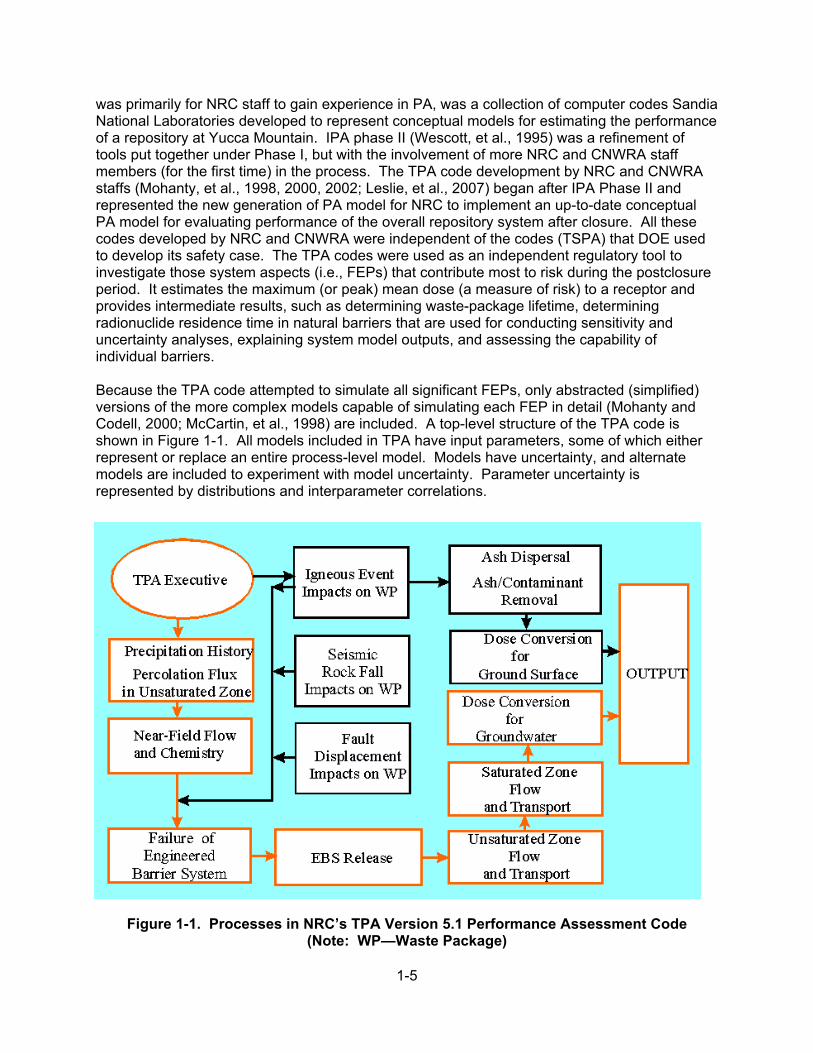
was primarily for NRC staff to gain experience in PA, was a collection of computer codes Sandia National Laboratories developed to represent conceptual models for estimating the performance of a repository at Yucca Mountain. IPA phase II (Wescott, et al., 1995) was a refinement of tools put together under Phase I, but with the involvement of more NRC and CNWRA staff members (for the first time) in the process. The TPA code development by NRC and CNWRA staffs (Mohanty, et al., 1998, 2000, 2002; Leslie, et al., 2007) began after IPA Phase II and represented the new generation of PA model for NRC to implement an up-to-date conceptual PA model for evaluating performance of the overall repository system after closure. All these codes developed by NRC and CNWRA were independent of the codes (TSPA) that DOE used to develop its safety case. The TPA codes were used as an independent regulatory tool to investigate those system aspects (i.e., FEPs) that contribute most to risk during the postclosure period. It estimates the maximum (or peak) mean dose (a measure of risk) to a receptor and provides intermediate results, such as determining waste-package lifetime, determining radionuclide residence time in natural barriers that are used for conducting sensitivity and uncertainty analyses, explaining system model outputs, and assessing the capability of individual barriers. Because the TPA code attempted to simulate all significant FEPs, only abstracted (simplified) versions of the more complex models capable of simulating each FEP in detail (Mohanty and Codell, 2000; McCartin, et al., 1998) are included. A top-level structure of the TPA code is shown in Figure 1-1. All models included in TPA have input parameters, some of which either represent or replace an entire process-level model. Models have uncertainty, and alternate models are included to experiment with model uncertainty. Parameter uncertainty is represented by distributions and interparameter correlations.

Figure 1-1. Processes in NRC’s TPA Version 5.1 Performance Assessment Code (Note: WP—Waste Package)

1-6

TPA is a Monte Carlo simulation code, although it was not always used in that way, as will be seen when other sampling methods are described. It can run hundreds to several thousand output realizations. For each realization, input parameter values are obtained by sampling from their probability distributions (along with correlation). Either random or stratified (e.g., Latin Hypercube) sampling methods are used (Rice and Mohanty, 2000). The latest version of the TPA code⎯TPA 5.1⎯has on the order of 1,000 parameters, of which 200–400 are typically sampled and 40–50 are cross-correlated to other sampled parameters. To include spatial heterogeneity in the near field, the rock volume including the repository is divided into vertical, columnar flow units called subareas. The subarea approach is used to improve computation time of the Monte Carlo simulations by expediently representing spatial variability in material properties and repository environmental conditions. The complicated volcanic stratigraphy is represented through a sequence of uniform layers that vary in thickness from subarea to subarea. These variations permit representation of spatial variations in topography, soil cover thickness, and fractures. Stratigraphic variations in each subarea permit incorporation of different material properties and the length of transport path both in matrix and fractures. In the far field, a streamtube approach is used to model movement of aqueous phase radionuclides from the repository horizon through the unsaturated and saturated zones, and ultimately to the receptor location. The transport model simulates a spectrum of transport processes, such as advection, dispersion, matrix diffusion, sorption, and decay of radionuclides. Heat generation, temperature evolution, and the resulting thermohydrological processes are computed for two thermal modes⎯high temperature and low temperature. In the high temperature mode, the temperature exceeds the boiling point of water and the processes of evaporation and condensation dominate the water flow rates through the fractures and the rock. Chemistry evolves with temperature and impacts the drip shield and the waste package environment for corrosion. Mechanical stresses and thereby the stability of the emplacement drifts also depend on the thermal load (in addition to in-situ and seismic stresses). Various submodels either compute or use abstracted results from detailed models for heat transfer, water–rock geochemical interactions, and refluxing of condensate water. Some of the key parameters defining the near-field thermo-hydro-chemical processes include (i) time-dependent temperatures (e.g., at the drift wall and waste package), (ii) relative humidity in the vicinity of the waste package, (iii) pH and chloride, (iv) and fluoride concentration of the water contacting the waste package and drip shield. Time dependency is considered when conducting uncertainty and sensitivity analyses. Two types of radionuclide source terms are considered: (i) radionuclides that either are dissolved in water or are carried as suspended colloidal particles and (ii) radionuclides that become airborne because of an extrusive volcanic event. In either case, the drip shield and the waste packages fail before such source terms are activated. The waterborne source term may result from undetected manufacturing defects in containers, failure due to corrosion, failure due to rockfall because of drift degradation, slip on an existing fault, or formation of a new fault. The TPA code estimates radionuclide release rates from the EBS based on spent fuel dissolution rates, radionuclide solubility limits, transport mechanisms out of the waste package, the water contact model, volume fractions of the spent fuel contacted by water, spent fuel particle sizes, and cladding failure. Radiological risk from extrusive igneous activity is estimated by modeling airborne release of radionuclides in the form of the ash–waste mixture into the atmosphere and eventual uptake of these radionuclides by the receptor. There are two versions of the igneous model: (i) the original ASHPLUME model assumes exposure by the receptor from airborne releases directly

1-7

and (ii) the newer TEPHRA model assumes both direct airborne exposure and also exposure from the remobilization and erosion of contaminated ash deposited in the watershed upstream of the RMEI. The time-dependent release of radionuclides to the water table from the extrusive event is computed as a function of the power and duration of the eruption, wind speed and direction, radionuclide areal densities on the ground surface, thickness of the ash blanket, leaching and erosion rates, and decay rates. Risk to the RMEI is then calculated by assuming the withdrawal of contaminated water from the saturated zone for drinking and irrigation purposes. Because of the low probability, it is computationally expensive to obtain the consequence of the extrusive igneous activity simultaneously with the undisturbed scenario. Therefore, a special method is used to combine the dose to an RMEI from the volcanic events with the results from the undisturbed scenario. Seismicity and climate change are included in the basecase model, which represents the undisturbed scenarios. A low-probability, high-consequence extrusive igneous event is the only event included in the disruptive scenario. The probability of occurrence of the scenario classes is used in calculating the combined risk curve from the undisturbed and disruptive scenarios. The TPA code has been used in calculating the effects of human intrusion (Smith, et al., 1999) and near-field criticality (Weldy, et al., 2001) through stylized calculations requiring different sets of parameters. 1.2.3 Performance Metrics Radiological protection of public health and the environment is a primary objective of a repository. The primary performance metric is the expected dose to an individual during the postclosure period. Expected dose reflects the traditional definition of risk (i.e., probability times consequences). For the HLW postclosure repository system, the risk is usually expressed in terms of a probability weighted dose, for comparison to the dose-based individual protection standard. Other performance metrics are more local to the system. These could be performance of individual barriers and intermediate outputs (also referred to as pinch points). Sensitivity and uncertainty analyses have been carried out with respect to these performance metrics. Overall, the natural system is expected to function as a barrier to the transport of radioactivity. The engineered system is expected to enhance the capabilities of the site to protect the public and the workers during the preclosure period, but would also function as a barrier to radionuclide release to the accessible environment in the post-closure period. 1.3 Report Structure Chapter 2 presents uncertainty analyses and their context for the definition of risk. Chapters 3 and 4 show a suite of sensitivity analysis techniques, both statistical and nonstatistical, that has been used in NRC’s PAs to identify the influential uncertain parameters driving performance uncertainty. Chapter 3 concentrates mostly on textbook statistical methods for sensitivity, whereas Chapter 4 concentrates on innovative methods NRC and CNWRA staffs developed. Chapter 5 describes how sensitivity and uncertainty analyses have been interpreted and used. Chapter 6 presents the NRC and CNWRA early sensitivity and uncertainty analysis activities. Chapter 7 presents a summary and conclusions, and Chapter 8 contains references. The appendix has some available computer routines for sensitivity analysis that are either in the public domain or are straightforward translations of some of the methods presented in Chapters 3 and 4 into the public domain “R” language (CRAN, 2011). Presenting these routines

1-8

allows the reader who is unfamiliar with sensitivity techniques to try some of the simpler methods without the need for specific proprietary software or computer platforms. Several terms are used throughout the report synonymously to maintain consistency with the papers, reports, and original work cited. However, there are subtle differences in a stricter sense. The term “parameters” is synonymous with “variables,” and “samples” is synonymous with “realizations.”

2-1

2 UNCERTAINTY ANALYSIS

2.1 Introduction

A quantitative risk assessment is a formalized calculation of risk from a process or event, generally used to support a regulation. Risk assessments require models, which are usually simplified representations of real systems (Kirchner, 2008). Models reflect uncertainty due to simplifying assumptions and uncertainty in the models’ parameters. Uncertainty is one of the most important parts of the quantification of risk. This report will describe a history of the U.S. Nuclear Regulatory Commission’s (NRC) experiences with risk assessment calculations, primarily for high-level radioactive waste (HLW) repositories, and the Yucca Mountain project in particular. It invokes some of the discussions and logic that NRC has used and developed over the last few decades, and will cover the following topics:

• Definitions of uncertainty and risk • Propagating uncertainty in models • Generating risk bases • Random sampling • Peak-of-the-mean criterion for risk • Risk dilution • Convergence of risk curve • Granularity

2.2 Risk and Risk Assessment

Risk will be defined for the case of repository licensing as either the “risk triplet” (Kaplan and Garrick, 1981; Callan, 1998) or as “probability times consequences.” In the current discussion, risk refers to “dose risk” (i.e., pertaining to the radiological exposure to an individual or population). The risk triplet definition poses the three questions: (i) What can go wrong? (ii) How likely is it? and (iii) What are the consequences?

Information derived from running performance assessment (PA) codes will automatically address the risk triplet. The probability times consequence calculation is used to generate a single curve of dose versus time by compiling the PA code results (i.e., combining the dose consequence at each instant of time over all realizations.) Because realizations are generally equally probable within a scenario, this is simply the average dose over all realizations.

The rationale for defining a mean dose curve has its basis in the distinction between high-dose and low-dose radiological response (Clark, 2008). High doses generally are a result of accidental exposure (e.g., nuclear reactor accidents, wartime exposure to nuclear weapons, or deliberate exposure due to medical treatment). If doses are high enough, then it is possible to see direct (“deterministic”) effects to the exposed individual.

Doses from a well-engineered repository would almost certainly be in a range far below those doses that would cause deterministic effects. The effects of low levels of radiation are usually treated as increasing the probability of a health consequence to the exposed individual. The increased health consequence could only be detected in a large population and could not be distinguished as causing direct harm to a particular individual. This increased risk is known as a

2-2

“stochastic” or random effect. Furthermore, the most used paradigm for low-dose response assumes that hazard to an individual or population is linearly proportional to absorbed dose (the “linear no-threshold” model).

If each realization of the PA calculations produces only a low dose (i.e., below the deterministic dose threshold), then the effect of each realization only adds to the overall stochastic risk to the subject individual or population. The overall risk, therefore, is proportional to the dose to that individual at each instant of time averaged over all possible outcomes (realizations), weighted by the probability of the outcome. The peak of the mean dose curve is usually chosen to compare the PA results to the dose criterion, e.g., 15 mrem/yr [0.15 mSv/yr] to the reasonably maximally exposed individual (RMEI). 2.2.1 Repository Risk Assessment The evaluation of repository performance involves the development and use of a PA computer model (e.g., TPA and TSPA) to simulate the most important factors of the prototype repository. The development of the model for the repository PA is usually pursued in the following order: (i) specify FEPs that should be evaluated as scenarios in the PA; (ii) develop adequate mathematical models of repository performance that can process the important phenomena under the assumed scenarios; (iii) develop input parameter distributions for the models; and (iv) develop the framework of the system model to handle input, output, Monte Carlo sampling, running of mathematical models, and analysis of results. Figure 2-1 illustrates the steps involved in the PA once the PA model has been developed. The first step is to sample the input parameters distributions for the PA models to generate a list or

Figure 2-1. Monte Carlo Modeling of Repository Performance

2-3

“vector” of parameters for each realization (typically, several hundred realizations). The sampled parameters are then run through the PA models to generate the performance measure such as dose to the RMEI. Finally, all evaluated realizations are combined to get a measure of risk to compare to the regulatory standards. 2.2.2 Uncertainty in the Context of Performance Assessment Uncertainty in dose calculations arises from many causes, including incomplete capture of physical processes in the consequence models used in the PA, incomplete knowledge of model parameters, and random events or stochastic processes. Each Monte Carlo realization of the PA model is used to calculate the effects of uncertainty in the parameters that determine the model outcome. Aleatory is the uncertainty in a parameter that comes about because the exact value cannot reasonably be known. Aleatory includes parameters associated with disruptive scenarios that are random or stochastic in nature, such as the time of occurrence of a volcano or earthquake, the intensity of a volcanic eruption, and the wind direction or speed at the time of a volcanic eruption. Although these parameters are physical attributes of the natural environment, long-term predictions of their values are unknowable in advance, at least by current scientific understanding. The best we can do is to characterize them in terms of probability distributions, e.g., wind roses for meteorological parameters or frequency statistics, such as the characteristic frequency of a Poisson distribution λ (yr-1) for earthquake recurrence. Epistemic uncertainty is the uncertainty in the value of a fixed, but uncertain parameter of the model. Examples of epistemic uncertainty are the values of physical properties, such as thermal conductivity of a rock at a particular location, and the frequency of volcanic eruption and earthquakes. Note that the time of occurrence of a volcanic eruption or earthquake is an aleatory parameter, but the frequency can still be an epistemic parameter. There are analogies between the evaluation of aleatory and other treatments in the physical sciences of stochastic behavior. Just two examples of aleatory are shown here for illustration, but there are many others. First consider the “representative elementary volume” or REV in groundwater hydrology. Flow of water through saturated porous sand on a microscopic level depends on the viscous flow around individual grains. Each flow path could theoretically be calculated if every last detail was known about the size of the grains and their orientation with respect to each other. The variability in the size and orientation of the grains is real, but practically unknowable, and is therefore aleatory. This problem is generally handled by averaging the properties of the porous medium “…over a small region of space⎯small with respect to macroscopic dimensions in the flow system but large with respect to the pore size” (Bird, et al., 1960). This approach essentially averages the aleatory uncertainty in the porous medium into a macroscopic property of the system, making the problem tractable. Another useful analogy, also from Bird, et al. (1960) is that of turbulent flow, which allows that observations must take into account temporal averages. Bird observes “(the equations of continuity and motion), if they could be solved, would give the instantaneous values of the velocity and pressure, which in turbulent flow are fluctuating wildly about their mean values … The equations of change can be averaged over short time intervals to get the ‘time-smoothed’ equations of change.” Bird is expounding on a similar recognition that there is real aleatory

2-4

variability in a turbulent flow system. Although the individual variations are interesting, only the average properties of the system are truly useful. NRC’s TPA code considers the following types of uncertainty: • Some aspects of uncertainty in seismicity and volcanism, namely the times of

occurrence, are treated as aleatory.

• Parameter distributions for most other factors are treated as epistemic uncertainty.

• Model uncertainty is captured by alternative conceptual models.

Spatial and temporal variability are treated in the TPA code, but generally are not sampled. For example, the repository is represented as a number of subareas, each with different physical properties and pathways to human exposure. Infiltration varies with time in an attempt to address climate changes.

2.2.3 Parameter Sampling In the case of NRC’s TPA code, there are several scenarios evaluated. In the nominal case, the computer models of the various phenomena that need to be simulated have both fixed parameters and uncertain parameters represented by probability distributions. The basis for assigning a constant value or a probability distribution to the parameter depends on various factors. For example, constant values are assigned to parameters that are either well characterized or have uncertainty ranges that do not significantly affect model results. Probability distributions are assigned to parameters not well known or where variability is sufficient to affect model results has been observed in data. Selection of the particular distribution type, such as normal, uniform, or beta, depends on the information available for the parameter and may involve either the best fit of data to a distribution or a reasonable assumption of the distribution type. 2.2.3.1 Distribution Functions for Parameters The probability density function (PDF) is the standard form in which uncertainties are represented in a probabilistic model. The PDFs need to be defensible especially because (i) too broad an uncertainty range may lead to risk dilution and (ii) too narrow an uncertainty range may indicate unwarranted confidence in the parameter range, thereby biasing the results. For a probabilistic model to be defensible and consistent, it requires a thorough and systematic examination of input parameters. It is also important to minimize the number of sampled parameters for the PA model. If the response is not expected to be sensitive to a certain parameter in the model, then the parameter can be assigned a constant value. Note that obtaining data to support estimation of PDFs is often one of the most expensive parts of risk analysis. 2.2.3.2 Developing Empirical Probability Density Functions Because PA is an inherently multidisciplinary activity, the Center for Nuclear Waste Regulatory Analysis (CNWRA®) and NRC staffs developed a questionnaire for all PA experts and process-level experts to understand the needs for PA model parameters.

2-5

This questionnaire was useful in obtaining information required to develop PDFs with appropriate levels of technical bases. It facilitated obtaining the required level of support with reasoned arguments. It also promoted a series of organized interactions between the process and system modelers to (i) ensure that a consistent set of standards were used in developing the PDFs and (ii) challenge process modelers to think more broadly and comprehensively. The questionnaire promoted information gathering for both sampled and nonsampled parameters. The process modelers were requested to provide • Qualitative/quantitative arguments • Level of original data used in developing the PDF • Documentation substantiating the choice of the PDFs

The following are some of the questions from the questionnaire on types and potential effects of uncertainty: • Is there no uncertainty (i.e., is the parameter value well known)?

• Are there random errors in measurement?

• Are there systematic or biased errors in measurement?

• Are there only scarce applicable data or measurements?

• Are extrapolations in time or space needed in conditioning the data for use in the

system model?

• Are underlying models, data, and understanding empirical? Is the theoretical support weak?

• Is there natural variability at different times?

• Is there natural variability from place to place?

• Is there imprecise understanding of the parameter or model?

• Are there potential correlations and dependencies that are not quantified?

Information gathering from process modelers and performance assessors through a questionnaire provided a systematic approach, which is key to obtaining a uniform description of uncertainty. It was important for the experts to understand the purpose of the PA model and its role in regulatory reviews before responding to the questions. It was observed that bringing process modelers on board early in the process is important for the information to be useful to performance assessors.

2-6

Parameter distributions generally apply to epistemic uncertainties and reflect the belief in the value of a constant but unknown quantity. The PDF expressing this degree of belief can be developed by several means, depending on the availability of actual parameter values:

• If there are sufficient data, the values of the parameter can be used to generate an empirical PDF directly.

• If data are available, but limited, the data can be combined with subjective knowledge or expert opinion to generate parameter distributions.

• If a parameter is a combination of several other parameters whose distributions are known, they can be combined probabilistically to generate a new distribution function. This can be done formally by analytical integration or probabilistically by Monte Carlo sampling of the base distributions.

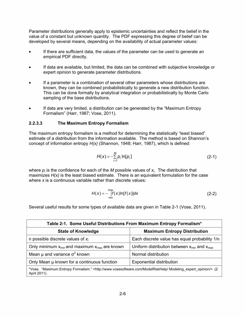
• If data are very limited, a distribution can be generated by the “Maximum Entropy Formalism” (Harr, 1987; Vose, 2011).

2.2.3.3 The Maximum Entropy Formalism The maximum entropy formalism is a method for determining the statistically “least biased” estimate of a distribution from the information available. The method is based on Shannon’s concept of information entropy H(x) (Shannon, 1948; Harr, 1987), which is defined:

]ln[)(1

i

M

ii ppxH −=

=(2-1)

where pi is the confidence for each of the M possible values of xi. The distribution that maximizes H(x) is the least biased estimate. There is an equivalent formulation for the case where x is a continuous variable rather than discrete values:

−=max

min)](ln[)()( dxxfxfxH (2-2)

Several useful results for some types of available data are given in Table 2-1 (Vose, 2011).

Table 2-1. Some Useful Distributions From Maximum Entropy Formalism*

State of Knowledge Maximum Entropy Distribution

n possible discrete values of xi Each discrete value has equal probability 1/n

Only minimum xmin and maximum xmax are known Uniform distribution between xmin and xmax

Mean μ and variance σ2 known Normal distribution

Only Mean μ known for a continuous function Exponential distribution

*Vose. “Maximum Entropy Formalism.” <http://www.vosesoftware.com/ModelRiskHelp/ Modeling_expert_opinion/> (2 April 2011).

2-7

Use of the maximum entropy formalism will always produce the most inclusive distribution justified by the available information. However, this is not always a desired property of the distribution used, because a wide distribution can lead to a problem known as “risk dilution” (i.e., the peak dose using the peak-of-the-mean approach can be smaller for a wide parameter distribution than if a narrower distribution was used).

2.2.3.4 Sampling From a Distribution Function For each realization in the PA model run, values of the variable model parameters are sampled from the chosen distribution functions. Sampling of a single parameter is illustrated in Figure 2-2. This figure illustrates the parameter distribution function as a Cumulative Distribution Function (CDF), with the value of the parameter on the abscissa and the CDF on the ordinate. Sampling of the value of the Parameter A is performed by generating a (pseudo) random number between 0 and 1 of the CDF, and then finding the value of A corresponding to the CDF value. When sampling multiple parameters, a modified sampling procedure, known as Latin Hypercube Sampling (LHS), is generally substituted for purely random sampling of the CDF. The LHS procedure forces a more even distribution of samples over the range of the parameters as illustrated in Figure 2-3 for two variables, but the method is valid for any number of sampled variables. 2.2.4 Parameter Correlations Frequently, the distribution of a parameter depends on the distribution of another parameter (i.e., the two variables are “correlated”). Figure 2-4 shows the correlation between two parameters with a coefficient of determination r2 = 0.68. The LHS sampling routine used in the TPA codes includes an algorithm to force correlations among two or more sampled variables. The correlation procedure is limited and can only force

Figure 2-2. Random Sampling From a Single Distribution Function

u1

u2

u3

A1 A2A3

Predefined CDFAny CDF

2-8

Figure 2-3. Latin Hypercube Sampling for Two Variables

-3 -2 -1 0 1 2 3

0.4

0.6

0.8

1.0

UZHPUDev

Sb

ArW

t%

Correlation between x[,2] and x[,38], R^2=0.68

Figure 2-4. Parameter Correlation Example

correlations in the rank of each set of sampled variables with the rank of another set. Also, the number of realizations must be at least as great as the number of sampled variables (Iman and Shortencarier, 1984). Parameters can also vary in time and space, and may not neatly fit into the categories of aleatory and epistemic uncertainty. As an example, the infiltration to the engineered barrier is likely to vary spatially because of the variability of the ground-surface elevation, and rock and soil properties. This problem is handled in the TPA code by classifying the waste packages according to how much infiltration they are expected to receive. Each class or “bin” of waste packages is characterized by the infiltration rate for the bin and the number of waste packages in the bin. The infiltration rate for each bin can also vary with time according to climate cycles.

Random value in bin

Evenly spaced bins along y-direction

2-9

2.2.5 Convergence of Model Results Monte Carlo techniques are used in the TPA for the probabilistic assessment of risk. Each Monte Carlo realization represents a possible outcome of the future effect of the repository. There are at least two ways to interpret the risk from the model output: (i) the “mean-of-the-peaks” approach takes the peak doses from the Monte Carlo realizations and draw conclusions from their ensemble (e.g., their mean) and (ii) the “peak-of-the-mean” approach takes the ensemble of all realizations and synthesizes a representative dose-versus-time curve (Codell and Esh, 2004; Mohanty and Codell, 2004). The mean-of-the-peaks approach is easy to understand and explain. However, the calculation of the mean-of-the-peaks dose allows an additional degree of freedom that may inadvertently overestimate risk. The peaks occur at different times, and therefore the mean may include contributions from peaks outside of a single person’s lifespan. This dilemma has been discussed previously in connection with the definition of the critical group (e.g., Corbett, 1988). NRC has adapted Method 2, taking the maximum value of the mean curve to represent the dose to the RMEI during the regulatory time period for the purpose of defining risk. NRC believes it to be the clearest and fairest definition of risk. However, the peak dose from each realization is also useful information. See for example the Strategic Partitioning of Assumption Ranges and Consequences (SPARC) methodology described in Section 4.10. Peak doses from each realization are also used most frequently in sensitivity analyses described in Chapters 3, 4, and 5. The choice of the Peak-of-the-Mean or the Mean-of-the-Peaks can affect sensitivity results. Generally, sensitivity analyses are conducted using peak doses, but the timing of the peak dose from each realization does not usually align with the time at which the peak-of-the-mean dose occurs. Examples that illustrate the effect of the use of peak doses to calculate sensitivities will be shown in Section 5.5. 2.2.6 Calculation of the Peak-of-the-Mean Dose Sampling and determination of risk sometimes differs for the nominal scenario and disruptive scenarios. For the nominal case, Monte Carlo sampling of the uncertain parameters yields the mean dose directly

r

N

r

r ptDtD )()(1

=

= (2-3)

where Dr(t) = dose rate as a function of time for the rth realization and pr = the probability of the realization. The PA models are run for multiple realizations to calculate the mean dose curve. For the nominal release scenario, in which processes like corrosion, radionuclide release, and radionuclide transport evolve slowly and predictably, this calculation usually requires several hundred realizations to produce a smooth mean dose versus time curve.1

1Note that the minimum number of realizations is usually set above the number of independent variables (parameters) of the model. The Latin Hypercube Sampling procedure requires that minimum number of samples for parameter correlations to work.

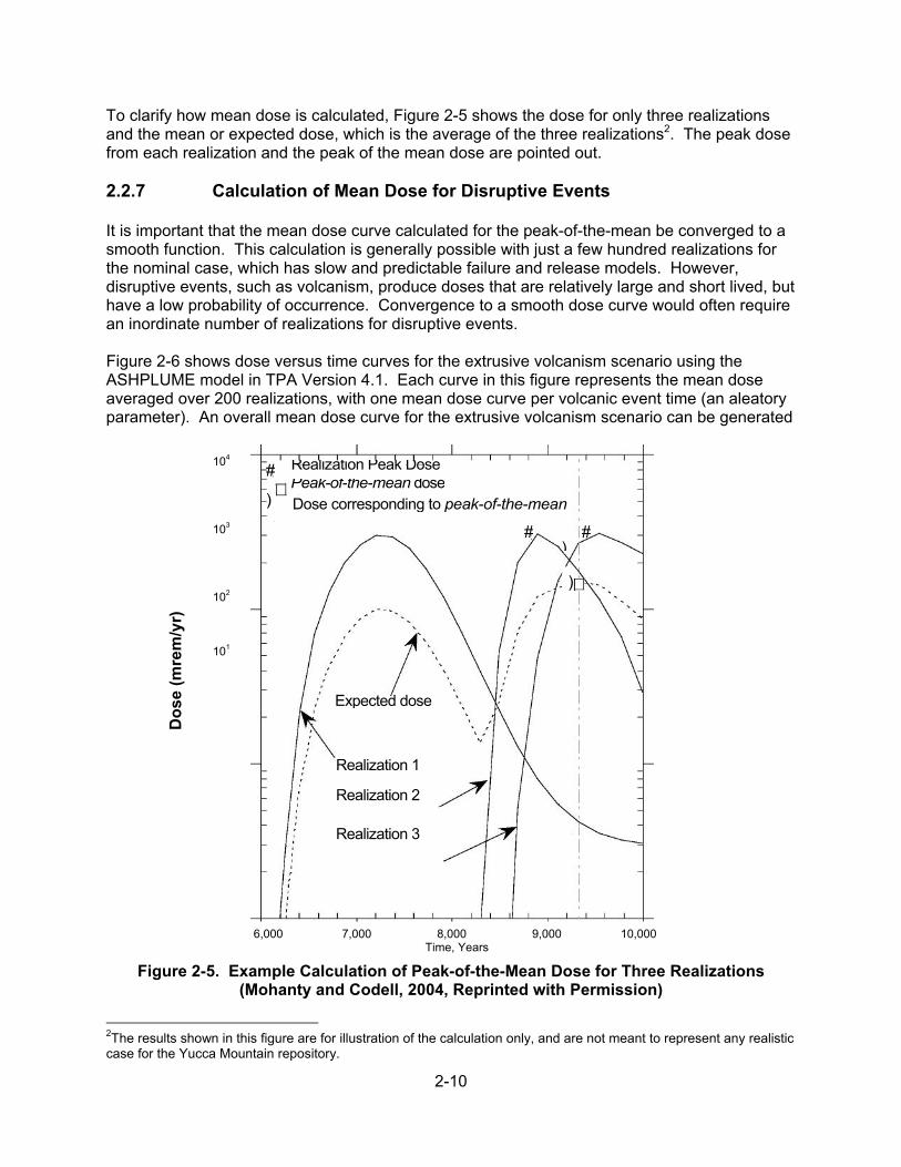
2-10

To clarify how mean dose is calculated, Figure 2-5 shows the dose for only three realizations and the mean or expected dose, which is the average of the three realizations2. The peak dose from each realization and the peak of the mean dose are pointed out. 2.2.7 Calculation of Mean Dose for Disruptive Events It is important that the mean dose curve calculated for the peak-of-the-mean be converged to a smooth function. This calculation is generally possible with just a few hundred realizations for the nominal case, which has slow and predictable failure and release models. However, disruptive events, such as volcanism, produce doses that are relatively large and short lived, but have a low probability of occurrence. Convergence to a smooth dose curve would often require an inordinate number of realizations for disruptive events. Figure 2-6 shows dose versus time curves for the extrusive volcanism scenario using the ASHPLUME model in TPA Version 4.1. Each curve in this figure represents the mean dose averaged over 200 realizations, with one mean dose curve per volcanic event time (an aleatory parameter). An overall mean dose curve for the extrusive volcanism scenario can be generated

Figure 2-5. Example Calculation of Peak-of-the-Mean Dose for Three Realizations (Mohanty and Codell, 2004, Reprinted with Permission)

2The results shown in this figure are for illustration of the calculation only, and are not meant to represent any realistic case for the Yucca Mountain repository.

6,000 7,000 8,000 9,000 10,000 Time, Years

)

#

) Dose corresponding to peak-of-the-meanPeak-of-the-mean doseRealization Peak Dose

Realization 1

Realization 2

Realization 3

Expected dose

# #)

Do

se (

mre

m/y

r)

104

103

102 101

2-11

Figure 2-6. Mean Conditional Dose Curves for ASHPLUME With Different Event Times by recognizing that a person living at time t’ will only be at risk from events taking place prior to t’. For the volcanism scenario, the average annual conditional dose at time t’ for an event at time te, )|'( ettD would be

)',()|'( eee tttfttD −= (2-4)

where f = dose at time t’-te (i.e., the time after the volcanic event happening at time te,) averaged over all random realizations. The individual curves in Figure 2-6 are examples of the function f. In that figure, the mean dose curves are shown to be a function of time after the event, as well as the time of the event. Assuming that extrusive volcanism has a constant annual probability pr of occurring in any year, the instantaneous dose to a person living at time t’ is the integration of all possible prior volcanic events multiplied by pr

−='

min

)',()'(t

tr dtfptD τττ (2-5)

where tmin = minimum time that the calculation of dose to the RMEI can occur, typically 100 years (i.e., the “administrative period” before which there would be intervention to control or eliminate dose, should an event occur, such as evacuation of the affected population). Because there are relatively few sampled parameters that describe the extrusive volcanism case, each new calculation of f for a fixed te requires only a modest number of realizations, typically 100 to 200. Equation (2-5) is evaluated by numerical integration using bilinear interpolation to get doses between the evaluated event times (Press, et al., 1992). Although this approach accounts for uncertainty of one aleatory parameter only—time of the occurrence of the volcanic eruption—it could treat other aleatory parameters such as wind speed and volcanic power.

2-12

Figure 2-7 shows the convergence of the mean dose curve using raw Monte Carlo sampling and the convolution3 procedure for the ASHPLUME model. This figure illustrates that the convolution procedure leads to much better convergence than raw sampling for this model. The convolution results seem to drift below the raw sampling results. This is a computational artifact of the increasing timestep length in the TPA code. Keeping the TPA timestep length constant eliminates this problem with the raw sampling result. Also shown in Figure 2-7 are the raw sampling results for the TEPHRA volcanism model used in TPA Version 5.1. In this case, raw sampling led to faster convergence than for the case of the ASHPLUME model. The reason for the faster convergence in the TEPHRA model case is that the processes in TEPHRA have a longer time constant than the ASHPLUME model, because the TEPHRA model also involves transport of contaminated soil and water.

Figure 2-7. Convergence of Mean Dose Curve Using Convolution and Regular Averaging of Realizations, ASHPLUME and TEPHRA Extrusive Volcanism Models

3The procedure is referred to as “convolution” because the function f in Eq. (2-5) was originally two functions, one

)(τf and the other )'( τ−tf . Later these were combined into a single function, but the name stuck.

2-13

2.2.8 Risk Dilution One potential disadvantage of the peak-of-the-mean approach is that it is subject to “risk dilution.” In general, the less that is known about a model parameter (epistemic uncertainty), the wider its probability distribution would be. Parameter-distribution estimation methods such as the “Maximum Entropy Formalism” (Harr, 1987), tend to specify wide, all-inclusive distributions when amounts of data are small. Although the use of these wide distributions tends to lead to the calculation of some realizations with large doses (because the models are evaluated sometimes in extreme regions of their parameter space), wide distributions can lower the peak-of-the-mean dose. The mean-of-the-peaks dose tends to give a more-pessimistic result for wide parameter distributions and therefore may not be subject to risk dilution (Rice, 2004). However, the mean-of-the-peaks dose may portray risk incorrectly. It is worthwhile for the risk analyst to be aware of large discrepencies in the risk measures; e.g., if there is a large difference between the peak-of-the-mean and the mean-of-the-peak dose estimates, then the analyst should endeavor to understand what is causing the difference. A graphic example of risk dilution using TPA 4.1 is shown in Figure 2-8 (Mohanty and Codell, 2004). In this example, the PDF is shown for two cases of the drip shield failure time, which is a simple sampled parameter in this model represented by a normal distribution. The two distributions have the same mean, but different variances. The narrower distribution gives a peak of the mean dose of 0.051 mrem/yr [5.1 × 10−4 mSv/yr] at 6,410 years, while the wider distribution gives a lower peak of 0.039 mrem/yr [3.9 × 10−4 mSv/yr] at 10,000 years. 2.3 Granularity and Upscaling of Performance Assessment Models The term “granularity” refers to a potential problem with PA codes, and simulations in general, where the degree of discretization affects the results of the study. For example, the repository

Drip Shield FailureTime, Years

Figure 2-8. Two Distributions for Drip Shield Failure Time (Mohanty and Codell, 2004, Reprinted with Permission)

2-14

will consist of many thousands of waste packages, but will be simulated by only a handful of “representative” waste packages. Random differences from package to package, and differences in the package environment from place to place in the repository, may not be captured adequately if the discretization is too coarse or “grainy.” This problem in general can also be called “upscaling,” because overall repository performance is of concern, rather than the behavior of individual waste packages. The importance of granularity depends on how the physical realities account for real spatial and temporal variability and uncertainty. For any given system, there will likely be real variability in the physical processes (e.g., for the fraction of waste contacted by infiltrating meteoric water, there will be variability in the infiltration from place to place, the protection afforded by the waste packages, and the changes to these terms over time). The potential problem of granularity can be handled by increasing the fineness of the discretization (e.g., increase the number of representative waste packages). Other examples would be (i) develop a theoretical relationship that can help stipulate the value of the sampled parameter that allows a single feature (e.g., a waste package) to represent the ensemble behavior or many waste packages or (ii) have a single travel path from the engineered barrier system to the RMEI represent the ensemble behavior of multiple pathways. 2.3.1 Example This example was derived for the Iterative Performance Assessment (IPA) Version 2 analysis (Wescott, et al., 1995), using models that were simpler than those used in subsequent versions of TPA. Furthermore, these models were geared toward compliance with 10 CFR Part 60 requirements for an HLW repository that were based on a cumulative release of radionuclides to the accessible environment over 10,000 years, whereas current regulations are based on maximum dose to a target individual. Nevertheless, this example illustrates how a reasonable choice for parameters for a source term model consisting of many waste packages could be approached using a single choice for an input parameter. Figure 2-9 shows the IPA Phase II model for the waste package. The effective volume of the waste package is determined by its original empty volume, or by the height of a corrosion hole.

Figure 2-9. Dissolve Radionuclide Release Model for Iterative Performance Assessment 2 (Wescott, et al., 1995)

2-15

It was assumed that (i) the jth waste package is a stirred tank with effective volume Vj and flow rate qj (Vj and qj can be different for each waste package within the realization); (ii) the waste packages fails at time tfail,j ,which can be different for each waste package within a realization; (iii) the waste package fills to the volume Vj, at which time there will be flow out at time tf,j ; (iv) the radionuclide has long half-life and no daughter products of importance (e.g., Np-237); (v) there is no cladding protection; (vi) the radionuclide release rate from the waste form is limited by solubility Cs; (vii) release from the waste package is by both advection at a rate qjC or by diffusion at a rate kC, where k is a constant for all waste packages within a realization; and (viii) diffusion starts when the waste package fails, but advection starts only after the fill time. The concentration within the waste package will be constant, Cs. The cumulative release carried out by the water for 10,000 years per waste package, ma, will be proportional to the flow rate through the waste package

ma,j = Cs q [10,000-tf,j ] (2-6) where tf,j = time to fill the waste package = Vj/qj. The cumulative diffusive release, md, is also proportional to the concentration

md,j = k Cs [10,000 – tfail,j ] (2-7) Where k is the proportionality constant for diffusion and the value of k is the same for all waste packages in the realization. The waste package failure time, tfail,j varies from waste package to waste package within the realization. The cumulative release of the radionuclide from all N waste packages over 10,000 years, M, is equal to the sum of the releases from each waste package following their filling, that is

=

−+−=N

ijfails

j

jjs tkC

qV

qCM1

, )]000,10()000,10([ (2-8)

The average cumulative release per waste package, <m>, is therefore the result of the previous equation divided by the number of waste packages, N:

<m> = Cs [10,000 <q> - <V> +10,000k – k<tfail>] (2-9) In other words, for the conditions stated, it would be possible to calculate the average release over 10,000 years within the realization for all waste packages using one simulated waste package and the mean values of q, V, and tfail, all calculated from their original sampled distributions. This convenient conclusion allows the calculation of the mean without having to sample a large number of waste packages. A similar calculation was performed for congruently released radionuclides (Wescott, et al., 1995). Systems that are more complicated than this simple example may not yield to techniques shown in this example, and may require the analysts to experiment with the fineness of the calculations (e.g., number of waste packages or transport pathways) to assure themselves that granularity is not a significant problem.

2-16

2.3.2 Conclusions on Uncertainty Analysis Uncertainty is a key part of repository risk assessment. The total system PA models take into account uncertainty in models and parameters. Most approaches have used Monte Carlo sampling to generate input for models and have analyzed the results to generate an approximation of risk of the repository. Empirical parameter distributions for the Monte Carlo sampling have been developed using elicitation from subject matter experts. Special procedures were developed to deal with convergence of the risk curve for short-lived but high-consequence disruptive events like volcanism. Throughout the history of NRC’s experience with repository risk assessments, the NRC staff have refined its models and understanding of how risk information should be generated, and how this information should be presented to best inform the regulators. The results of the PA models go beyond the nominal definition of risk as the peak-of-the-mean dose curve to also look at such things as the effect of failures in the multiple barrier system. Problems that can be associated with the propagation of uncertainty though the PA models include risk dilution caused by overly inclusive parameter distributions and granularity caused by too-coarse discretization of the model. The analyst’s awareness of potential pitfalls in developing the risk basis is an important aspect of any risk assessment. It is therefore useful to analyze the uncertainty analysis results from many angles; e.g., compare the peak-of-the-mean to the mean-of-the-peaks, assess intermediate outputs from the models rather than being concerned only with the final result, and determine whether or not the fineness of the calculations is sufficient.

3-1

3 SENSITIVITY ANALYSIS

3.1 General Considerations in Sensitivity Analysis

Performance assessment (PA) models for waste repositories, like any conceptual models, are abstractions of physical reality that attempt to simulate processes that lead to release of radionuclides and exposure to the environment, especially humans. Sensitivity analysis, as applied here, is a methodology to determine the importance of the various parts of the PA to the modelers’ results. This allows the modeler to focus their efforts to improve the PA. 3.1.1 Sensitivity to Alternative Models Model results can be sensitive to the choice of the model and submodels themselves, or their parameters. If there are multiple, plausible submodels to emulate a phenomenon (e.g., the release rate of a radionuclide from the waste form), then the PA results may be sensitive to the choice of the model. There are several options for dealing with model uncertainty, including 1. The most plausible model could be selected as the only one evaluated

2. Each submodel could be used in an alternative PA evaluation

3. All models could be carried forward in the PA analysis, giving weights to each alternative

according to its plausibility

Option 1 fails to give credit to alternative conceptual models. However, including all alternative submodels for multiple parts of the PA can prove to be impractical because of the many permutations that would have to be evaluated. Usually, the most important alternative models are evaluated to keep the workload within reasonable limits. 3.1.2 Use of Intermediate Results To Determine Model Importance The PA models, such as TPA, are a combination of submodels that are generally run serially (i.e., the output of one submodel, such as the source term, becomes input to the next submodel, such as groundwater flow and transport). Once a combination of plausible submodels is assembled into the PA, intermediate results from the submodels can be useful to determine their importance to the overall performance. Intermediate results, such as the failure rate of waste packages, radionuclide inventory still present within the various barriers, release rates to and from the barriers, and the key causes of barrier failures, can help an experienced analyst to understand the final overall performance. 3.1.3 Use of Barrier or Component Failure Analysis Repositories are always based on the robust principle of multiple barriers (i.e., the failure of a single barrier, such as the waste package should not lead to unacceptable hazard to the target exposed individual). A useful analysis using the PA models is to model the artificial total failure of barriers and observe the effect on the target individual of the hypothetical failure. This can be repeated for failure of multiple, or even all, barriers. The analysis can lead to the modeler concentrating on improving the reliability of models for those barriers that greatly affect the outcome. Artificial total failure may not be a reality and, if it happens, the probability of occurrence can be expected to be very low. Therefore, it is incumbent on the analyst to clearly

3-2

communicate that the purpose of turning component functionality off is only to facilitate the analysis, and in most instances this may not be a reality for any repository system. 3.1.4 Parameter Sensitivity Analysis In general, a sensitive parameter is defined as one that produces a relatively large change in the output variable (e.g., peak dose) for a change in the input parameter within the range of uncertainty. A major goal of the sensitivity analyses presented in this report is to determine the parameters to which peak dose for the simulation period shows the most sensitivity. Typical PAs have hundreds of parameters sampled from their probability distributions. Parameter sensitivity analysis finds those parameters that make the largest contribution to the dose outcome, or the variability in the dose. 3.2 Traditional Techniques for Parameter Sensitivity Sensitivity methods can be classified broadly as either statistically based or nonstatistically based, both of which have been used in the U.S. Nuclear Regulatory Commission (NRC) PAs. NRC staff traditionally use statistically based methods that rely on the Monte Carlo results generated from the uncertainty analyses. Statistically based methods rely on some form of random sampling of input parameters to generate a set of responses from the PA models. They then use statistical hypothesis testing to analyze the relationships between the input parameters and the responses to make inferences about the most sensitive input parameters. Most of this section will be devoted to statistical techniques. Nonstatistical sensitivity methods exercise the models specifically to address the sensitivity. Examples of nonstatistical sensitivity techniques are the Morris method, Fourier Amplitude Sensitivity Technique (FAST), and Factorial Design of Experiments (Mohanty, et al., 1999a; Lu and Mohanty, 2001). Most sensitivity analysis methods in this report used peak dose from each realization as the output variable because it was convenient to do so, and this result is most likely to demonstrate sensitivity relationships. Alternatively, the sensitivity methods could have used the dose from each realization taken at the time that the peak-of-the-mean occurs. Using the later definition rather than the peak dose from each realization was shown to sometimes rank the importance of the parameters in a different order, as illustrated in Section 5.5. 3.2.1 Statistical Sensitivity Analysis Based on Monte Carlo Sampling This section describes statistical techniques used to determine which input parameters in the TPA codes NRC and the Center for Nuclear Waste Regulatory Analyses (CNWRA®) developed from Iterative Performance Assessment (IPA) Phase 1 (Codell, et al., 1992) to TPA Version 5.1 (Leslie, et al., 2007). The output from the TPA code is given by yj, which is a function of the random parameters, xi, deterministic parameters, dk, and model assumptions, am

yj = f(x1,j,x2,j,…,xI,j, dk, am) (3-1) where j represents the jth of N realization and I is the total number of sampled parameters in the model. It is assumed that the behavior of the system is simulated by appropriately sampling the random parameters and then computing the system output, yj, for each realization of the

3-3

parameters. To outline a method for analyzing simulation output, identify important random parameters, and develop understanding of their relationship to the output, it is assumed that the decisions about appropriate model assumptions and fixed parameters have been made a priori. As a result, the dependence of y on fixed parameters and model assumptions is not considered further and focus is on the dependence of the output on the sampled parameters. 3.2.1.1 Developing and Manipulating Model Results for Sensitivity Analysis Model results are compiled from running the PA code and are presented in their original form in terms of a vector of the dependent variable y, (e.g., peak dose and a matrix of the sampled variables x.) Sensitivity analyses are performed on either the original values of x and y, or this information may be first altered by transformations to enhance the sensitivity calculations. 3.2.1.2 Variable Transformations and Their Attributes

The correlation between input and output variables in statistical methods can often be enhanced by transforming the variables. Transformations are used to (i) eliminate dimensionality of the variables, (ii) reduce the role of points at the tails of the distributions, and (iii) properly scale the resulting sensitivities to the variability of the input variables. However, transformation of the dependent variable (usually peak dose), can skew the results in an undesirable way because the risk, being based on the average dose, is weighted heavily by the largest doses. Therefore, the sensitivities should reflect what matters most to the risk, and give weights proportional to the doses. Although transformations of the dependent variable often will improve the goodness of fit in the sensitivity analysis, in general they should only be applied to the independent variables. NRC and CNWRA staffs have used the following transformations for sensitivity analyses: Normalization In normalization, the input variable, xi, is transformed by dividing it by its mean value (or another baseline value such as the median)

i

ii

X

XX =*

(3-2)

Normalized variables are dimensionless and are scalar multiples of their baseline values. Dimensionless variables allow the comparison of sensitivities to other independent variables with different dimensions.

Sensitivity measures based on normalized variables describe only the relative change in the dependent variable (peak dose) to changes in the model parameters. Although normalization allows a useful measure of sensitivity, it does not consider the ranges of the variability of the independent and dependent variables (see details under Standardization).

Rank Transformation

Rank transformation, a dimensionless transform, replaces the value of a variable by its rank (i.e., the position in a list that has been sorted from largest to smallest values). Analyses with ranks tend to show a greater sensitivity than results with untransformed variables. If

3-4

the distribution of doses is skewed toward the low end, which is usually the case, rank transformation of the dependent variable can give unfair weights to lower doses.

Logarithmic Transformation

For situations in which input and output variables range over many orders of magnitude, it may be advantageous to perform analyses on the logarithm of the variables instead of on the variable values themselves. The log transformation is also valuable for creating regression equations, where the subprocesses of the model multiply each other to form the output variable. For the present situation in which the dose calculation results from radionuclide releases from the waste form, transport through the geosphere, and uptake by humans, the processes are indeed largely multiplicative rather than additive. Log transforms, therefore, tend to give better fits to the Monte Carlo results than untransformed variables, but again at the expense of unfairly weighting the smaller doses if the dependent variable is also transformed. The log transformation may be used in conjunction with normalization.

Scaled-Power Transformation The scaled-power transformation is similar to the logarithmic transformation, but often allows a closer approach to normality. For a variable, ν, and power, p (p not equal to 0), the scaled-power transformation is (Cook and Weisberg, 1994)

p

pp )1()( −= νν (3-3)

For p = 0, Eq. (3-3) is indeterminate (i.e., 0/0). However, it can be shown by expanding p in an exponential power series that the scaled-power transformation reduces to the logarithmic transformation. A typical procedure for selecting p is to step through a range of values of the p in small increments and compare the shape of the resultant scaled distribution to the shape of a normal distribution. After each calculation of the new shape of the distribution, the Lilliefors test for normality (Bowen and Bennett, 1988) would be applied. The exponent yielding the best fit to the normal distribution is then chosen to scale the variable under consideration. Standardization The independent and dependent variables can be standardized by subtracting the mean and dividing by the standard deviation

x

ii

xxx

σ−

=* (3-4)

Sensitivity measures based on standardized variables (standardized sensitivities) have the advantage of considering the range of the independent variable. Direct linear regression with standardized variables properly weights all doses. Standardized variables can be greater or less than zero; hence, they cannot be used directly in the regression analyses using the log-transformed variables. Instead, the standardized sensitivities can be derived from sensitivities based on logs of the normalized variables

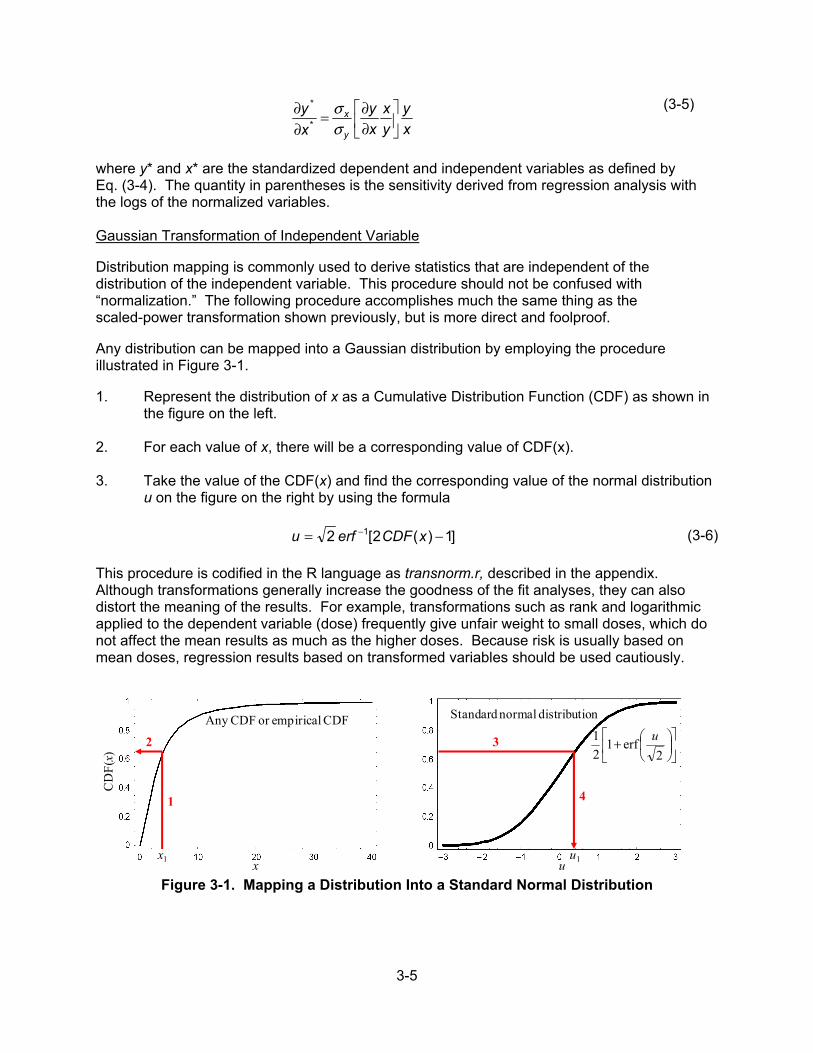
3-5

x

y

y

x

x

y

x

y

y

x

∂∂=

∂∂

σσ

*

* (3-5)

where y* and x* are the standardized dependent and independent variables as defined by Eq. (3-4). The quantity in parentheses is the sensitivity derived from regression analysis with the logs of the normalized variables. Gaussian Transformation of Independent Variable

Distribution mapping is commonly used to derive statistics that are independent of the distribution of the independent variable. This procedure should not be confused with “normalization.” The following procedure accomplishes much the same thing as the scaled-power transformation shown previously, but is more direct and foolproof.

Any distribution can be mapped into a Gaussian distribution by employing the procedure illustrated in Figure 3-1.

1. Represent the distribution of x as a Cumulative Distribution Function (CDF) as shown in the figure on the left.

2. For each value of x, there will be a corresponding value of CDF(x).

3. Take the value of the CDF(x) and find the corresponding value of the normal distribution

u on the figure on the right by using the formula

]1)(2[2 1 −= − xCDFerfu (3-6)

This procedure is codified in the R language as transnorm.r, described in the appendix. Although transformations generally increase the goodness of the fit analyses, they can also distort the meaning of the results. For example, transformations such as rank and logarithmic applied to the dependent variable (dose) frequently give unfair weight to small doses, which do not affect the mean results as much as the higher doses. Because risk is usually based on mean doses, regression results based on transformed variables should be used cautiously.

Figure 3-1. Mapping a Distribution Into a Standard Normal Distribution

x1

Any CDF or empirical CDF

x

CD

F(x)

1

2

u1

Standard normal distribution

u

+

2erf1

21 u3

4

3-6

3.2.2 Regression Methods

3.2.2.1 Single Linear Regression on One Variable

The most common test for parameter sensitivity is based on the correlation between two variables, under the assumption that they would plot as a straight line. For a single independent variable x and

dependent variable y, one could find the linear relationship by regression methods (Draper and Smith, 1998) with intercept a and slope b

bxay += (3-7) Linear regression of the output variable with respect to each of the input parameters can give a quantitative measure of the correlation through the coefficient of determination, R2, which is defined

−

−−=

ii

iii

yy

fyR 2

2

2

)(

)(1 (3-8)

where yi is the dependent variable data, fi is the straight line fitted value corresponding to the independent variable xi, and y is the mean value of the yi values.

This measure can be misleading, however, in cases where the dependencies are not linear or monotonic. Even when the output variable is linearly dependent on the input variable, linear regression of Monte Carlo results using only one of the sampled parameters may fail to show unambiguous correlation because other sampled parameters that affect the output are varying at the same time and the fitted model is clearly underspecified (i.e., the results depend on more than one variable).

The coefficient of determination is small for most variables in the analysis of TPA results and is not necessarily a good indicator of the importance of the variables. A better indication of influence is to determine the probability that the slope of the linear regression line is significantly different from zero. The t-test is generally used to determine, with a specified confidence level, that an estimated parameter value differs from another value. A parameter, xi, is deemed influential if there is a specified (e.g., 95 percent) confidence that the slope of its regression curve, mi, is different from zero (Benjamin and Cornell, 1970). This test is often referred to as the Pearson test.

The statistic of the slope of a single-variable regression line is defined as

2

2,

S

Snmt xi

ii = (3-9)

where

ti — t-statistic for regression coefficient mi mi — estimated value of regression coefficient i (i.e., slope of the best-fit line for dose

versus the independent variable, xi) S — estimated standard deviation of dose

3-7

Si,x — estimated standard deviation of the independent variable, xi n — number of samples

The critical value of ti to ensure 95 percent confidence that mi differs from zero for these conditions is 1.96 (Mason, et al., 1989). Equation (3-9) is used, therefore, to determine whether the absolute value of the t-statistic for each independent variable is greater than 1.96 (i.e., the probability of rejecting the null hypothesis) (H0⎯the correlation between x and y is zero is p<0.05). If not, the null hypothesis is rejected.

The t-statistic was used for the single-variable regressions and multiple linear regressions. This test is presented in slightly different formats in two “R” routines in the Appendix: the routines ttest.r and cortestkps.r.

Two similar regression tests are the Kendall’s “tau” test and Spearman’s “rank correlation” test, both of which use the ranks of x and y rather than the values themselves (MathSoft, Inc., 1993). These methods are presented in the R routine cortestkps.r in the appendix.

3.2.2.2 Stepwise Multiple Linear Regression

Stepwise multiple linear regression (stepwise regression) determines the most influential input parameters according to how much each input parameter reduces the residual sum of squares (Helton, et al., 1991). The form of the regression equation is

y = m 1 x 1 + m 2 x 2 +…+ m i x i +…+ m n x n + b (3-10)

where

y — dependent variable xi — independent variables m — regression coefficients b — intercept

The regression coefficients, mi, are the partial derivatives of the dependent variable with respect to each of the independent variables.

The regression coefficients, mi, are measures of the linear sensitivity of y to input xi (Draper and Smith, 1998). The stepwise algorithm calculates improvement in regression for each sampled parameter in the order that gives the greatest reduction first. To implement the procedure, a multiple linear regression model is fitted to the data in an iterative fashion. In the regression model, R2, the coefficient of determination indicates the fraction of variability in the data explained by all the variability in the model (Zimmerman, 1991). The sequence in which the inputs are selected is a useful measure of their uncertainty importance, as is the increment in R2 they produce. Figure 3-2 represents the output of a stepwise regression procedure, showing the reduction in residual sum of squares as parameters were added (Codell, et al., 2001).

There are several methods for determining which parameters are most important in the stepwise regression technique. The “forward” method adds parameters one at a time to maximize the improvement in fit of the model according to the R2 value. The “backward” method subtracts parameters one at a time to determine the effect on R2. A third method, Akaike Information Criterion (AIC), does not use hypothesis testing as other regression

3-8

Figure 3-2. Effect of Stepwise Regression of Peak Dose on Residual Sum of Squares (Codell, et al., 2001)

methods, but offers a balance between accuracy and complexity of a model (Akaike, 2011). However, AIC is very slow compared to forward or backward stepwise methods.

The NRC staff have used several versions of stepwise regression, including Iman, et al. (1980), forward and backward stepwise routines in R language (Conesa, et al., 2005), and one AIC stepwise routine in the normal statistical routines incorporated in R. These routines are discussed further in the appendix.

3.2.2.3 Sensitivity for Non-Monotonic Relationships

Regression-based methods are most useful for monotonic relationships (i.e., the dependent variable y only increases or decreases with increasing value of the independent variable x). When this is not the case, regression based methods are at a severe disadvantage. A non-monotonic relationship can be highly correlated, but have a low correlation coefficient.

Kleijnen and Helton (1999) expound on several statistical tests that are useful for determining the sensitivity of parameters that do not show a monotonic dependence.

Location of y Dependent on x

This set of sensitivity methods is based on measures of central tendency of the dependent variable y with the central tendency of the independent variable x. Either the mean or median of the values of x and y can be used as the measure of central tendency. The data are subdivided into classes of the independent variable x, usually with each region having an equal number of data points. Then the measure of central tendency for x and y is calculated within each region

3-9

and compared to the other regions to determine whether they have the same or different values of central tendency. If the mean is used for the measure of central tendency, then the Analysis of Variance (ANOVA) F test is commonly used to test for equivalence. If x and y are replaced by their ranks, then the Kruskal-Wallis test is substituted for the ANOVA F test. If the measure of central tendency of x and y is the median, then the partitioning is both in terms of classes of the independent variable x and the two classes of the dependent variable y (i.e., y either greater than or less than the median value of y). The chi-square statistic would be used to determine the sensitivity if the median of x and y are used as the measure of central tendency. Dispersion of y Dependent on x These tests are similar to those using the measure of central tendency, but instead measure the spread of y with changing values of x. They use either the variance of y or the interquartile range of y, y0.75 – y0.25 (i.e., the value of y at the 75th percentile minus the value of y at the 25th percentile.) The test that uses the variance is based on the same classification of x. However, the interquartile test divides the y values into three classes: above, within, or below the interquartile range. Distribution of y Dependent on x This test is used to determine whether the distribution of y is dependent on the distribution of x (i.e., to determine whether y is statistically independent of x). The independent variable x is divided into nx classes as before, but in this case, y is also divided into ny classes. Each class of x or y has approximately the same number of data points. The partitioning of x and y into nx and ny classes partitions the x/y data into nx times ny cells. The chi-square test for contingency tables is then used to determine whether there is any dependence of the distribution of y on the distribution of x.

All of these tests are included in the computer code PATTRN (Shortencarier and Helton, 1999) and described in the appendix.

3.2.3 Nonparametric Methods

Several nonparametric tests are included in NRC’s sensitivity repertoire. These include the Kolmogorov-Smirnov (K-S) test, the Sign test, and the Wilcoxon Rank Sum test. Nonparametric tests differ from regression tests because they do not require the assumption that the data have prespecified functional forms (e.g., normal).

3.2.3.1 The Kolmogorov-Smirnov Test

The K-S test determines whether a set of samples was drawn from a given distribution (Bowen and Bennett, 1988). This test is used to determine whether a sampled parameter is influential by comparing the distribution Sn(x) of a subset of the parameter, corresponding to the values from the highest 10 percent (or other range) of the peak dose realizations, to the completely specified theoretical distribution of that parameter, P(x), usually represented by 100 percent of the samples. This is done by comparing the CDFs of both distributions and determining the largest absolute difference, D, as illustrated in Figure 3-3. The significance of the K-S test was determined at the 95 percent confidence level. The difference D is compared to the statistic for 95 percent confidence. For the

=

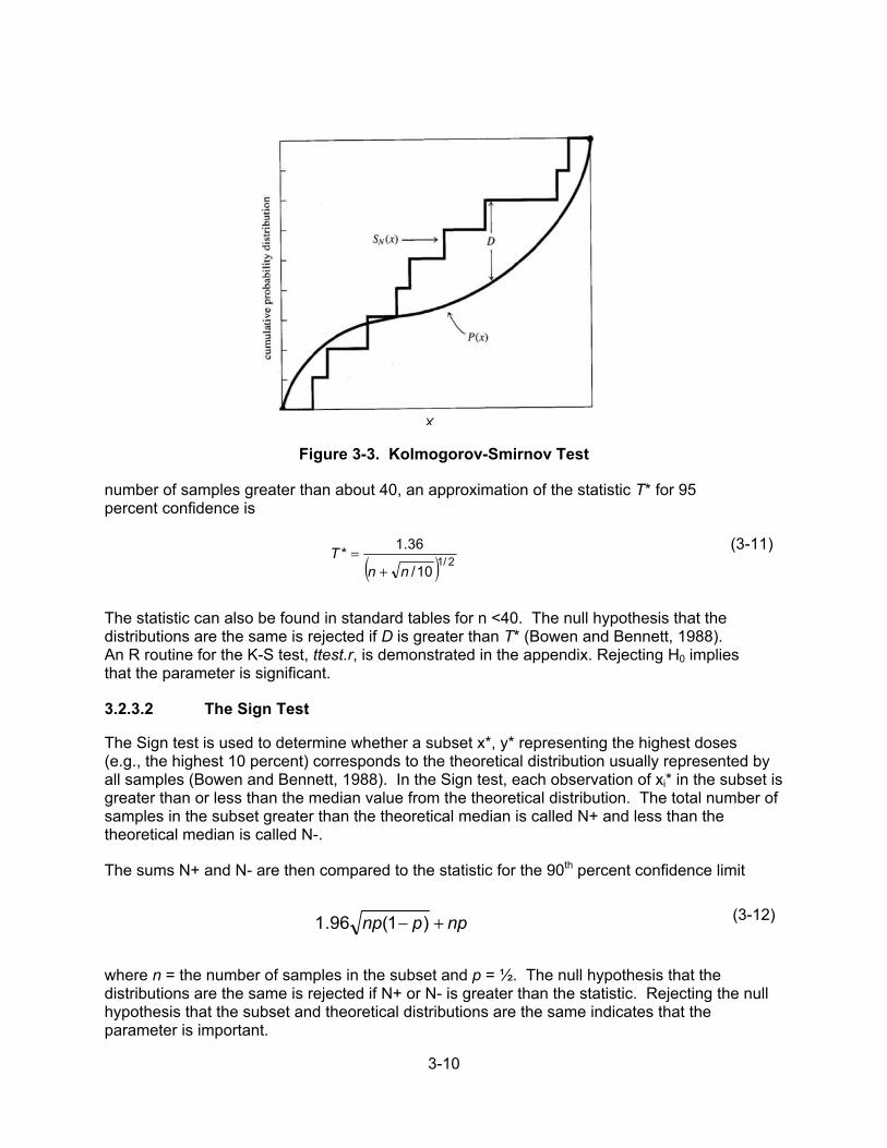
3-10

Figure 3-3. Kolmogorov-Smirnov Test

number of samples greater than about 40, an approximation of the statistic T* for 95 percent confidence is

( ) 2/110/

36.1*

nnT

+=

(3-11)

The statistic can also be found in standard tables for n <40. The null hypothesis that the distributions are the same is rejected if D is greater than T* (Bowen and Bennett, 1988). An R routine for the K-S test, ttest.r, is demonstrated in the appendix. Rejecting H0 implies that the parameter is significant.

3.2.3.2 The Sign Test

The Sign test is used to determine whether a subset x*, y* representing the highest doses (e.g., the highest 10 percent) corresponds to the theoretical distribution usually represented by all samples (Bowen and Bennett, 1988). In the Sign test, each observation of xi* in the subset is greater than or less than the median value from the theoretical distribution. The total number of samples in the subset greater than the theoretical median is called N+ and less than the theoretical median is called N-.

The sums N+ and N- are then compared to the statistic for the 90th percent confidence limit

nppnp +− )1(96.1

(3-12)

where n = the number of samples in the subset and p = ½. The null hypothesis that the distributions are the same is rejected if N+ or N- is greater than the statistic. Rejecting the null hypothesis that the subset and theoretical distributions are the same indicates that the parameter is important.

X

3-11

The significance of the Sign test was determined at the 90 percent confidence level to be consistent with previous total system PA analyses. Also, NRC staff practice was to combine the results of the Sign test and the K-S test so that both tests must pass to demonstrate the significance of the parameter. 3.2.3.3 The Wilcoxon Rank Sum Test As with the K-S and Sign tests, the Wilcoxon Rank Sum test is used to determine whether the distribution of the parameter values corresponding to high doses is different from the distribution of the parameter for the remaining doses. The procedure tests the null hypothesis that the means of the two distributions are the same. If m is the number of samples in the high-dose category, and n the sample size for the remaining dose, then the test is conducted by combining the samples from the two populations and ranking the combined sample. The test statistic for the Wilcoxon test is the sum of the ranks, R(xi), assigned only to the high dose category:

=

=m

i

ixRW1

)(' (3-13)

This statistic is compared to tabulations for the Wilcoxon Rank Sum test. Special attention must be paid to ties in the ranking. An R procedure for the Wilcoxon test, wilcox.r, is described in the appendix (Bowen and Bennett, 1988).

Nonstatistical Sensitivity Methods⎯Differential Analysis Technique

Regression analysis of the Monte Carlo results can only determine the most influential parameters when those parameters also have large enough regression coefficients that they are distinguishable from the confounding effects of the simultaneous sampling of all other independent variables. Differential analysis does not use Monte Carlo sampling results. It determines sensitivity unambiguously because it deals with changes in only one independent variable at a time. Differential analysis determines sensitivity of parameters only at local points in parameter space and does not consider the wide range of parameter variations like the Monte Carlo method does.

Differential analysis tests were conducted through multiple deterministic runs in which a single input parameter was changed by a known amount compared to its initial baseline value, while all other input parameters were held at a baseline value. The baseline value for this report is a sampled value for the input parameter. The sensitivity of a performance measure (in this case, peak dose for the simulation period) to a parameter is estimated as the first derivative of the performance measure with respect to that parameter, as approximated by finite differences

i

ii

i xxyxxy

xy

Δ−Δ+= )()(

δδ

(3-14)

Usually δxi is small (e.g., 10 percent of the parameter value). These estimates of sensitivity are local (i.e., the value of the derivative may change at different points in the sample space). To partially alleviate this concern, the derivate may be evaluated at several points in the sample space. In the analyses presented herein, the derivative is transformed in one of two

ways to allow comparison of sensitivity coefficients between parameters with different units. The first transformation is normalization, as described in Section 3.2.1.2.

3-12

y

x

x

yS i

ii δ

δ= (3-15)

Because Si does not account for the range of the input parameter, a second transformation of the derivative is also performed. In the second transformation, the derivative is multiplied by the standard deviation of the input parameter distribution. Baseline cases were run with input parameter values set at seven random points within each parameter distribution range selected using the Latin Hypercube Sampling (LHS) technique. Seven points may not cover the whole space, but this limitation was imposed to keep computational resources within a reasonable budget.

Other methods that do not rely on Monte Carlo sampling results are covered in Chapter 4.

3.3 Conclusions

Parametric sensitivities mostly can be determined by statistical hypothesis testing, using the results from the Monte Carlo uncertainty analyses. A variety of regression and nonparametric statistical tests can be applied for sensitivity. Special techniques are sometimes required when the response of the performance measure is not monotonic with respect to the input parameter. Differential analysis calculates the sensitivities directly by numerical differentiation at local points in parameter space and does not use the Monte Carlo results from the uncertainty analysis. Other, more advanced methods that require specially directed runs of the PA model, as well as barrier and component analyses, are covered in the next chapter.

4-1

4 ADVANCED AND SPECIAL-CASE SENSITIVITY TECHNIQUES 4.1 Introduction This chapter discusses some of the more advanced sensitivity methods that the U.S. Nuclear Regulatory Commission (NRC) and the Center for Nuclear Waste Regulatory Analyses (CNWRA®) staffs either developed or applied to waste management applications. This chapter covers both parametric sensitivity as well as barrier and component sensitivity. 4.2 Cumulative Distribution Function Sensitivity Analysis Method The Cumulative Distribution Function (CDF) sensitivity analysis was developed at Southwest Research Institute® through an internal research and development project to conduct sensitivity analysis with complex and computationally intensive problems represented by large numbers of parameters (i.e., referred to here as a large-N problem) (Mohanty and Wu, 2000, 2001; Wu and Mohanty, 2006). The method was later used to identify influential parameters in the TPA code involving hundreds of sampled parameters. This method is a sampling-based sensitivity analysis method used as a screening method to identify and rank parameters that are key uncertainty drivers. The sensitivity measure is defined as the derivative of a response CDF, at a given response threshold, with respect to a statistical parameter (such as mean or standard deviation) of an input random parameter. The method uses hypothesis-testing for acceptance limits, introduced for the first time (to the best of knowledge of the developers of this method) in the sensitivity analysis literature. In general, CDF sensitivities can be computed based on finite-difference approximations, which would require two or more probabilistic analyses per input distributional parameter. Clearly, the computational requirements depend on the number of random parameters. Because every probabilistic TPA analysis typically requires thousands of deterministic runs, a CDF sensitivity analysis would require hundreds of thousands of deterministic TPA runs, which can be computationally overwhelming. While there are a few existing statistical methods that are more efficient, including screening experiments and stepwise regression (Montgomery, 2000), and reliability approaches such as using most-probable-point-based importance factors (Madsen, et al., 1986), these existing methods do not provide error bounds or confidence levels to the computed sensitivity estimates. In general, they are more suitable for well-behaved functions—functions that are singly connected, continuous, and not highly nonlinear, such as having sharp peaks/valleys or not differentiable. For large-N systems, it may be difficult to know or test whether the performance functions are well or ill behaved. With lack of error or confidence measures, the existing methods may produce inaccurate sensitivity results without giving warnings.

The elements of the CDF-based sensitivity analysis method include (i) CDF sensitivities are computed using a subset of random samples (input and response) generated from TPA runs; (ii) random errors of the calculated sensitivity measures can be managed by controlling the number of random samples; (iii) errors of the computed sensitivities are, for the most part, independent of the number of random parameters; and (iv) random parameters are classified (as significant or insignificant) and ranked using statistical tests of hypothesis. The first element is important because it implies that additional TPA runs are not needed, though more samples may be desirable to reduce sampling errors. The second and third elements are the reasons the CDF sensitivity method is particularly suitable for large-N problems. The last element provides useful visual plots for classification and ranking using confidence limits.

4-2

A key feature of the CDF-based sampling method is that it is not limited to well-behaved functions. The calculated sensitivities can focus on any response/performance level, and the results asymptotically approach the exact values with increasing numbers of samples. The following section summarizes two CDF sensitivity measures with confidence limits.

4.2.1 Sampling-Based Cumulative Distribution Function Sensitivities

The two CDF-based sensitivity measures are defined as the derivatives of a response CDF, at a given response threshold, with respect to the mean and standard deviation of an input random parameter.

Denote the CDF of a random parameter X at X = x as ( )XF x and the probability density

function (PDF) of X as ( )fX x . The CDF of a response Y can be represented as

0 0( ) ( ( ) ) ( )Yp F y P Y y f dΩ

= = < = XX ... x x (4-1)

where ( , , ... )1 2 n= X X XX and Ω is the domain in X that satisfies the performance-function

constraint 0( )Y y<X . The integral in Eq. (4-1) provides a useful formulation to compute the

sensitivity of CDF at any desirable percentile by varying 0y together with Ω . Before the CDF

sensitivity can be calculated, the CDF needs to be computed by a suitable method. If Monte Carlo (MC) is used, 0Number of samples with [y < y ]/Number of MC samples.p ≈

The

samples associated with 0[y < y ] are the samples to be used for sensitivity analysis, as

illustrated in Figure 4-1 for a well-behaved ( )Y X function with a single input parameter. For ill behaved functions, the domain Ω may be more complex, such as having multiple, disconnected regions. However, it would not pose any problems in identifying 0[y < y ] samples

using Monte Carlo.

Figure 4-1. Sampling-Based Cumulative Distribution Function Sensitivity Analysis Method

4-3

From Eq. (4-1), the sensitivity of p at ( )y op F y= with respect to a distribution parameterθ (mean

or standard deviation) can be formulated as (Karamchandani, 1990)

p f d∂ ∂∂θ ∂θΩ

= X... x (4-2)

The partial derivative /p θ∂ ∂ represents the sensitivity to be computed. Eq. 4-2 can lead to an expectation function suitable for averaging using random samples

Xpfp p

Ef p

f ff

dxθ θ θ ΩΩ

= = ⋅∂∂

∂ ∂ ∂ ∂

X

X

X

X

... (4-3)

in which ( / )f pX is a properly scaled density function such that

1 fp

dxΩ

= X... (4-4)

Thus the expectation function [ ].E Ω in Eq. (4-3) is supported in the Ω domain and zero

elsewhere. By varying 0y , and therefore Ω , the sensitivities covering a wide range of CDF of Y

can be computed as a by-product of a single Monte Carlo simulation results.

The mean sensitivity, denoted as Sμ , and the standard-deviation sensitivity, denoted as Sσ , are

defined as

//i

i i

p pSμ∂∂μ σ= (4-5)

//i

i i

p pSσ∂∂σ σ= (4-6)

where iμ and iσ are, respectively, the mean and the standard deviation of the random parameter iX . The standard deviation is used as a normalization factor to make the sensitivity measures dimensionless and more appropriate for variable ranking.

For the benefit of creating confidence limits that are applicable for different distributions, each Xi

can be transformed to a standard normal variate, ui, by using

1( ( ))ii X iu F x−= Φ (4-7)

Where ui has zero mean and unit standard deviation and 1 (.)−Φ is the inverse normal CDF. It

can be shown that

[ ]i iS E uμ Ω= (4-8)

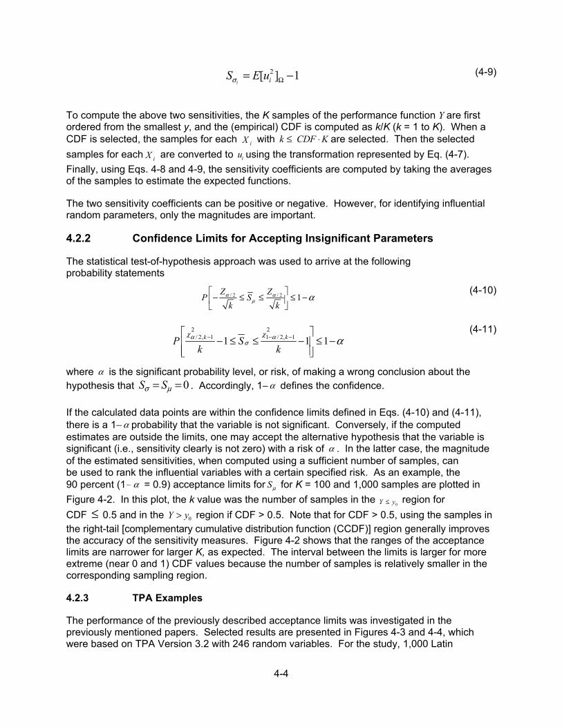
4-4

2[ ] 1i iS E uσ Ω= − (4-9)

To compute the above two sensitivities, the K samples of the performance function Y are first ordered from the smallest y, and the (empirical) CDF is computed as k/K (k = 1 to K). When a CDF is selected, the samples for each iX with k CDF K≤ ⋅ are selected. Then the selected

samples for each iX are converted to iu using the transformation represented by Eq. (4-7).

Finally, using Eqs. 4-8 and 4-9, the sensitivity coefficients are computed by taking the averages of the samples to estimate the expected functions.

The two sensitivity coefficients can be positive or negative. However, for identifying influential random parameters, only the magnitudes are important.

4.2.2 Confidence Limits for Accepting Insignificant Parameters

The statistical test-of-hypothesis approach was used to arrive at the following probability statements

/ 2 / 2 1Z ZP S

k kα α

μ α − ≤ ≤ ≤ −

(4-10)

2 2/ 2, 1 1 / 2, 11 1 1k kP Sk k

α ασ

χ χα− − −

− ≤ ≤ − ≤ −

(4-11)

where α is the significant probability level, or risk, of making a wrong conclusion about the hypothesis that 0S Sσ μ= = . Accordingly, 1− α defines the confidence.

If the calculated data points are within the confidence limits defined in Eqs. (4-10) and (4-11), there is a 1− α probability that the variable is not significant. Conversely, if the computed estimates are outside the limits, one may accept the alternative hypothesis that the variable is significant (i.e., sensitivity clearly is not zero) with a risk of α . In the latter case, the magnitude of the estimated sensitivities, when computed using a sufficient number of samples, can be used to rank the influential variables with a certain specified risk. As an example, the 90 percent (1!α = 0.9) acceptance limits for Sμ for K = 100 and 1,000 samples are plotted in

Figure 4-2. In this plot, the k value was the number of samples in the 0Y y≤ region for

CDF ≤ 0.5 and in the 0Y y> region if CDF > 0.5. Note that for CDF > 0.5, using the samples in the right-tail [complementary cumulative distribution function (CCDF)] region generally improves the accuracy of the sensitivity measures. Figure 4-2 shows that the ranges of the acceptance limits are narrower for larger K, as expected. The interval between the limits is larger for more extreme (near 0 and 1) CDF values because the number of samples is relatively smaller in the corresponding sampling region.

4.2.3 TPA Examples

The performance of the previously described acceptance limits was investigated in the previously mentioned papers. Selected results are presented in Figures 4-3 and 4-4, which were based on TPA Version 3.2 with 246 random variables. For the study, 1,000 Latin

4-5

Figure 4-2. Examples of Acceptance Limits (The Sampling Sensitivity Is Inside the Limits if a Parameter Is Insignificant)

Figure 4-3. Cumulative Distribution Function Sensitivities Sμ for Top 10 Parameters

Having Highest Average

4-6

Figure 4-4. Cumulative Distribution Function Sensitivities Sσ for Top 10 Parameters

Having Highest Average Hypercube samples were used. The estimates of Sμ and Sσ for the top 10 influential variables

are plotted in Figures 4-3 and 4-4, respectively. The Sμ results were better (i.e., more accurate and discriminatory in separating unimportant

from important parameters) and were validated by rerunning the analysis and examining the reduced variances after replacing the identified top 10 parameters by their mean values. The standard deviations of the performance were computed after holding at fixed values (mean values) 0, 1, 2, 3, 4, and 10 topmost influential parameters (based on Sμ , see Figure 4-3); the

remaining 246 input parameters were allowed to be sampled within their ranges of variation. The correlation coefficients were unchanged. The standard deviation of the performance is plotted in Figure 4-5. Each point on the curve represents the output from an additional 250 runs using a Latin Hypercube Sampling (LHS) simulation. When the top parameter was fixed at its mean value, there was a significant drop (approximately 94 percent reduction) in the standard deviation. The curve remained flat after fixing variables 2 and 3 because the top three parameters were correlated. The performance standard deviation dropped to about 2 percent after fixing the top 10 variables. The results verified that both Sμ and Sσ correctly identified the most influential random variables.

4.2.4 Correlation Issue

The sensitivity analysis methodology preserves the statistical correlations between input random parameters. For correlated '

iX s , the transformation using Eq. 4-7 will produce

correlated iu variables and their sensitivities will be correlated as well. The correlations,

however, will not result in mistakenly removing a significant random parameter. It may, however, fail to identify a spurious random parameter that has no real impact on the

4-7

Figure 4-5. Performance Standard Deviation Before and After Fixing 1, 2, 3, 4, and

10 Most Influential Variables at Mean Values

performance, but has a strong correlation with one or more truly significant random parameters. Noting that by definition a spurious parameter should have a small sensitivity, it can be identified by computing / iy x∂ ∂ (at some selected points such as the mean value) while holding other parameters.

4.2.5 Sample Size Requirement

Usually the sample size cannot be predetermined but may be adaptively determined using the following convergence criteria:

• To identify the influential random variables, stop adding samples when the sensitivities of the top n (n is a number determined by the analyst) significant variables violate the test of hypothesis.

• To rank the variables, stop when the ranking of the top n most influential variables stabilizes.

• To obtain accurate sensitivities, stop when the sensitivities of the top n influential variables fluctuate within an error bound.

4.2.6 Summary

The CDF sensitivity method features (i) using random samples to calculate sensitivity at any designated level of the CDF of the response and is not limited to the mean value; (ii) using acceptance limits, derived from test-of-hypothesis, to classify significant and insignificant random parameters; and (iii) using two sensitivity measures to rank the influential random parameters. Because no approximation is needed in this method either in the form of the performance functions or the type of continuous distribution functions representing input parameters, the sampling-based CDF sensitivity approach provides a reliable alternative that can handle ill-behaved or highly nonlinear functions with nonnormal parameters. Also, because

4-8

the sample size needed does not depend on the number of random parameters, it is particularly suitable for complex models, such as the TPA models, that have large numbers of random parameters, relatively few of which are significant. For TPA problems where random samples have already been obtained, the CDF sensitivity method can provide useful sensitivity information without additional TPA runs. 4.3 Genetic Algorithms With Cascaded Variable Selection Genetic algorithms can be used to search for synergistic sets of input parameters that are good predictors of model output (Davis, 1991). Genetic algorithms are based on processes found in biological evolution. The input vector of sampled parameters is altered by adding, subtracting, and mutating parameter values to find optimal sets of parameters that fit the data most closely. How well the variable set can explain the output can be evaluated with a logistical regression or a neural network. Genetic algorithm analysis was performed using neural network software (NeuralWare, 2001). Neuralworks Predict® is an add-in to Microsoft® Excel® that can be used to build neural networks. Sampled parameters along with the pertinent output variable (e.g., peak total dose, dose at a particular time, dose for a particular radionuclide at a particular time) were exported from the Performance assessment (PA) model to Excel, and then a neural network was built using Neuralworks Predict. The neural network itself was not used directly in the analysis. Instead, the variable selection algorithms were used to select the most important parameters needed to develop a neural network to predict the output. Parameters can be preselected using a cascaded genetic algorithm (CGA) approach. CGA uses a series of runs based on different initial conditions to prune out parameters that are consistently rejected by different invocations of the genetic algorithm. This results in variable sets that are consistent. Neuralworks Predict® evaluates sampled values of input parameters and selected output result (e.g., peak total dose, peak dose of a selected radionuclide). It selects a set of inputs to predict output and has a utility in predicting output quantified as the “importance factor,” which is the frequency at which a parameter is selected by the genetic algorithm, and can be taken as a measure of parameter sensitivity. 4.3.1 Example—Shallow Land Disposal of Saltstone The example problem is a PA model for shallow land disposal of a saltstone waste form that NRC staff developed using GoldSim software (GoldSim Technology Group, LLC., 2004). The problem and models are simpler but similar to those for high-level radioactive waste (HLW) repositories. The PA model contains abstracted submodels that represent degradation of the engineered cap; oxidation and physical degradation of the saltstone; transport of radionuclides in the unsaturated zone (UZ), saturated zone (SZ), and surface water; and a dose assessment. An iterative approach was used to develop risk insights. The initial stage of the simulation was mainly to identify which of the more than 250 sampled parameters were most likely to influence risk to a member of the public. The initial simulation was facilitated by representing parameter uncertainties by wide probability distributions. Individual realizations of the basecase were examined in detail to ensure the results were reasonable and consistent with physics and the conceptual model. The top three parameters identified by the genetic algorithm all pertain to the

4-9

degradation of the waste form. It is less clear whether parameters other than the top three significantly affect the model output. Next, the initial list of sampled parameters was reduced to a list of approximately 100 by eliminating those parameters that were sampled, but not actually used, in the model calculations or that were associated with radionuclides that did not contribute more than 0.001 mrem/yr [1 × 10−5 mSv/yr] to the peak mean dose. The neural network was then rebuilt with the shortened list of sampled parameters, because the ability of the algorithms to identify the parameters driving the output is enhanced when the input list is shorter. The selection algorithm with the reduced set identified six parameters, all with a high frequency. The parameters pertain to the degradation of the waste form, the quantity of radionuclides directly consumed in drinking water, or the dilution of contaminants in the SZ during transport and transport time. From a physical standpoint, the parameters selected are in strong agreement with the analysts’ conceptual understanding of the performance of the disposal system. As a further test of the power of this method, the genetic algorithm was tried with the same TPA Version 4.1 results used in Section 3.4 with results presented later in Tables 5-1 and 5-2. Using modified raw data,1 the Predict code successfully identified 6 of the 10 parameters identified in Table 5-2. Screening out realizations that had zero doses (about 200 of the 512) identified 7 of the 10 parameters. Using both sets of results identified 8 of the 10 parameters. 4.3.2 Conclusions The techniques employed here appear to better identify important parameters than traditional techniques, especially when the data are noisy. However, the analyst’s understanding of the initial results of the parameter screening was useful to the final analysis. Screening out of spurious parameters that the analyst determined could not have been important was a key to developing a good understanding of the importance of the model parameters. Results with the Predict® code were impressive when applied to the same data set used for determining important parameters in the TPA Version 4.1 10,000-year case, although the data set was somewhat less noisy because it was prescreened due to size limitations of the Excel program. NRC experience with applying genetic algorithm–CGA combination technique for sensitivity analysis suggests the technique is quite powerful for identifying key input parameters while eliminating spurious correlations, a common problem with large data sets of many sampled parameters. The method works well with the inherent “noise” in PA model output. The algorithm also uses variable transformations on the sampled parameter distributions as well as the output of the model to address the nonlinearity in the PA models.

1Data were screened for this case because Microsoft Office® Excel® Version 2003 used in the Predict code was limited to 256 columns. Therefore, parameters 13–59 (rockfall), 79–120 (seismic failure), and 308–330 (faulting and volcanism) were eliminated from the data set. Screening of the results confirmed that these parameters would not materially affect the outcome.

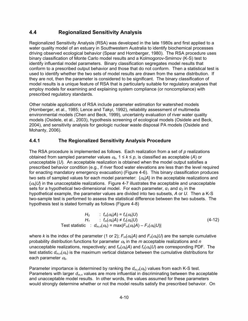
4-10

4.4 Regionalized Sensitivity Analysis Regionalized Sensitivity Analysis (RSA) was developed in the late 1980s and first applied to a water quality model of an estuary in Southwestern Australia to identify biochemical processes driving observed ecological behavior (Spear and Hornberger, 1980). The RSA procedure uses binary classification of Monte Carlo model results and a Kolmogorov-Smirnov (K-S) test to identify influential model parameters. Binary classification segregates model results that conform to a prescribed output behavior and those that do not conform. Then a statistical test is used to identify whether the two sets of model results are drawn from the same distribution. If they are not, then the parameter is considered to be significant. The binary classification of model results is a unique feature of RSA that is particularly suitable for regulatory analyses that employ models for examining and explaining system compliance (or noncompliance) with prescribed regulatory standards. Other notable applications of RSA include parameter estimation for watershed models (Hornberger, et al., 1985; Lence and Takyi, 1992), reliability assessment of multimedia environmental models (Chen and Beck, 1999), uncertainty evaluation of river water quality models (Osidele, et al., 2003), hypothesis screening of ecological models (Osidele and Beck, 2004), and sensitivity analysis for geologic nuclear waste disposal PA models (Osidele and Mohanty, 2006). 4.4.1 The Regionalized Sensitivity Analysis Procedure The RSA procedure is implemented as follows. Each realization from a set of p realizations obtained from sampled parameter values αk, 1 ≤ k ≤ p, is classified as acceptable (A) or unacceptable (U). An acceptable realization is obtained when the model output satisfies a prescribed behavior condition (e.g., if river flood water elevations are less than the level required for enacting mandatory emergency evacuation) (Figure 4-6). This binary classification produces two sets of sampled values for each model parameter: {αk|A} in the acceptable realizations and {αk|U} in the unacceptable realizations. Figure 4-7 illustrates the acceptable and unacceptable sets for a hypothetical two-dimensional model. For each parameter, α1 and α2 in the hypothetical example, the parameter values are divided into two subsets, A or U. Then a K-S two-sample test is performed to assess the statistical difference between the two subsets. The hypothesis test is stated formally as follows (Figure 4-8)

H0 : fm(αk|A) = fn(αk|U) H1 : fm(αk|A) ≠ fn(αk|U)

Test statistic : dm,n(αk) = max|Fm(αk|A) – Fn(αk|U)| (4-12)

where k is the index of the parameter (1 or 2); Fm(αk|A) and Fn(αk|U) are the sample cumulative probability distribution functions for parameter αk in the m acceptable realizations and n unacceptable realizations, respectively; and fm(αk|A) and fn(αk|U) are corresponding PDF. The test statistic dm,n(αk) is the maximum vertical distance between the cumulative distributions for each parameter αk. Parameter importance is determined by ranking the dm,n(αk) values from each K-S test. Parameters with larger dm,n values are more influential in discriminating between the acceptable and unacceptable model results. In other words, the values assumed for these parameters would strongly determine whether or not the model results satisfy the prescribed behavior. On

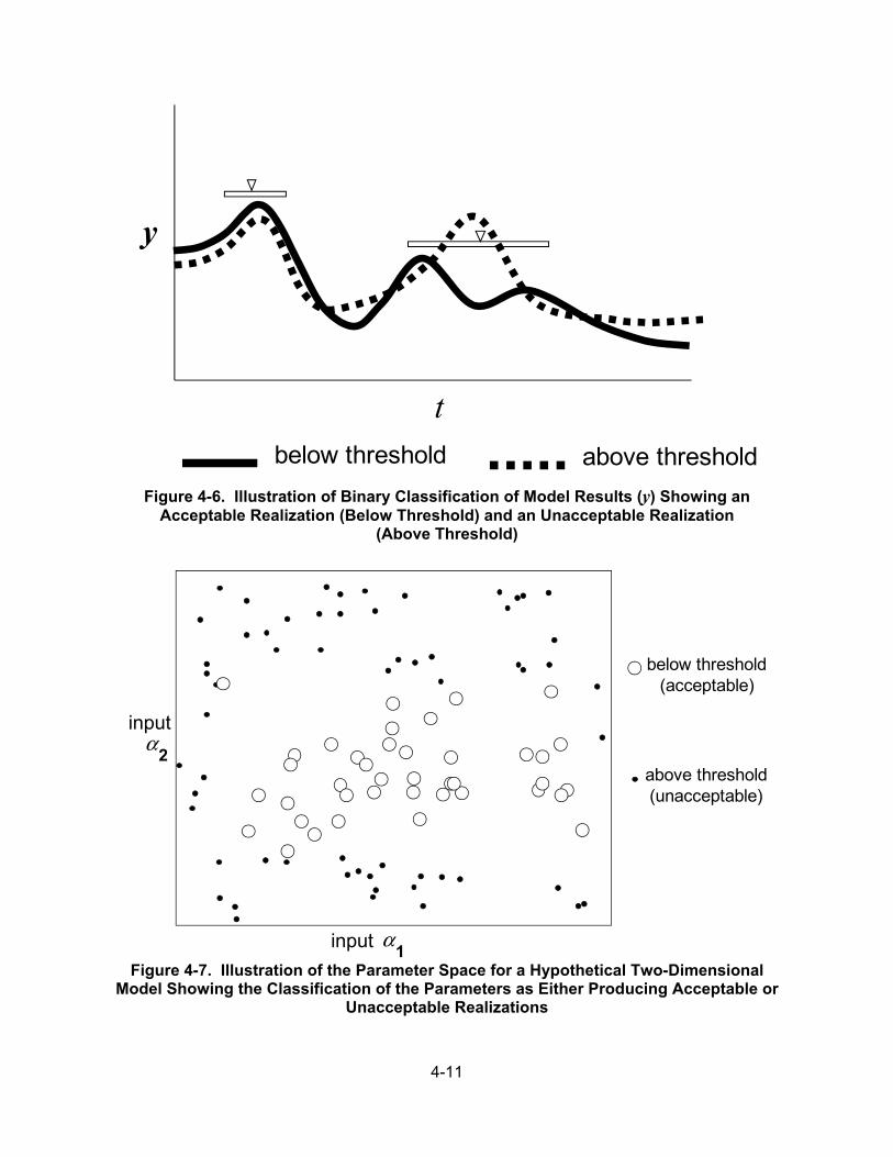
4-11

Figure 4-6. Illustration of Binary Classification of Model Results (y) Showing an Acceptable Realization (Below Threshold) and an Unacceptable Realization

(Above Threshold)

Figure 4-7. Illustration of the Parameter Space for a Hypothetical Two-Dimensional Model Showing the Classification of the Parameters as Either Producing Acceptable or

Unacceptable Realizations

y

tbelow threshold above threshold

α1

α2

below threshold(acceptable)

above threshold(unacceptable)

input

input

4-12

Figure 4-8. Illustration of the Two-Sample Kolmogorov-Smirnov Test for a Two-Parameter Model. dm,n Is the Maximum Vertical Distance Between the Cumulative

Distributions for Each Parameter

the other hand, parameters with smaller dm,n values are deemed less influential because any sampled value is almost equally likely to produce acceptable or unacceptable model results. However, the K-S two-sample test, as described in Eq. (4-12), does not always provide a reliable basis for comparing multiple parameter rankings for the same model. This is because dm,n depends on the sizes of {αk|A} and {αk|U}, (i.e., m and n, respectively) which may differ if the parameter samples are changed or a different behavior condition is prescribed. To obtain an unbiased comparison of the parameter rankings, the dm,n value for each parameter is converted to the standard K-S variate (zKS) as follows (Conover, 1999)

zKS(αk) = dm,n(αk) × [m × n/(m + n)]0.5 (4-13)

The significance level chosen for the analysis is adopted as the criterion for determining the influential parameters of the model. For the K-S distribution, the 5 percent significance level corresponds to zKS = 1.36. Thus, parameters with zKS(αk) greater than 1.36 are identified as important to discriminating between acceptable and unacceptable model results. 4.4.2 Example RSA is demonstrated with a version of the Total-system Performance Assessment (TPA) code (Mohanty, et al., 2002). The RSA procedure is used to determine parameter importance conditioned on specified dose thresholds. Specifically, the analysis seeks to identify influential parameters that discriminate between model results below (acceptable) and above (unacceptable) thresholds defined by the 10th-, 25th-, 50th- (median), 75th-, and 90th-percentile doses. For this example, the TPA code generates 500 random realizations based on distributions assigned to 400 model parameters, including 52 correlated pairs of parameters. Figure 4-9 shows the five dose curves derived from these realizations, which define the thresholds for the binary classification of model results. For each threshold, the model

α1

α2

below threshold [ A ] above threshold [ U ]

input input

dm,n

dm,n

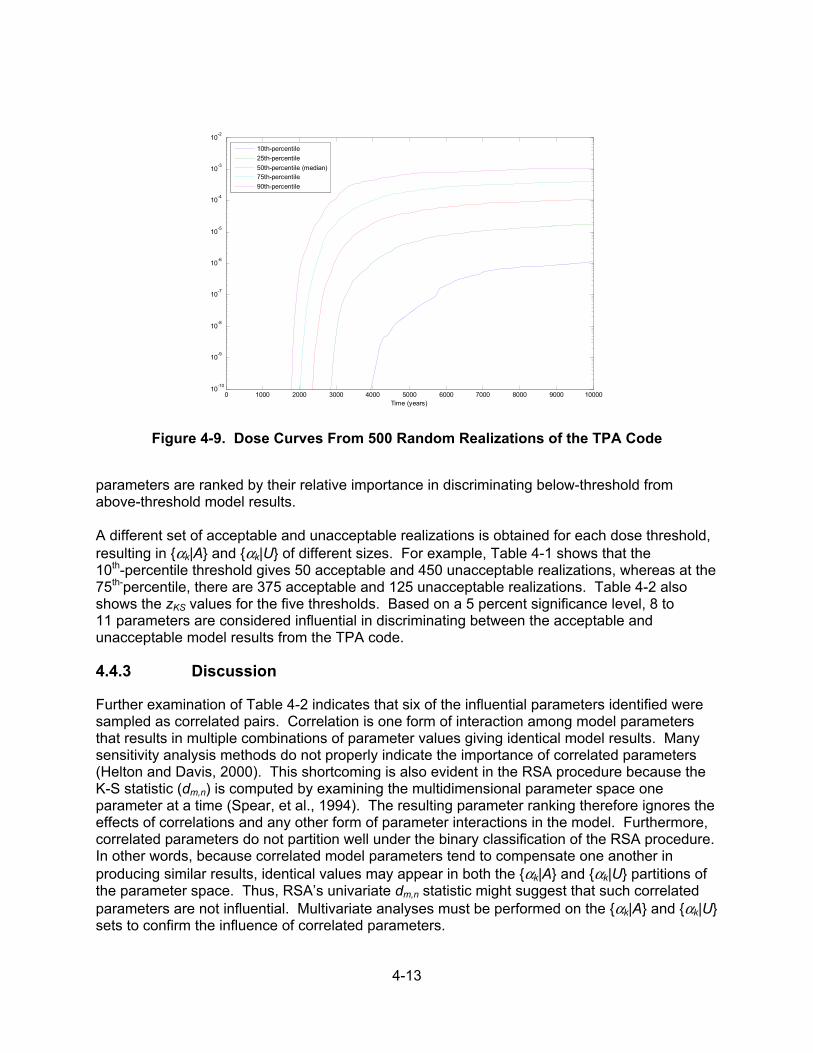
4-13

Figure 4-9. Dose Curves From 500 Random Realizations of the TPA Code

parameters are ranked by their relative importance in discriminating below-threshold from above-threshold model results. A different set of acceptable and unacceptable realizations is obtained for each dose threshold, resulting in {αk|A} and {αk|U} of different sizes. For example, Table 4-1 shows that the 10th-percentile threshold gives 50 acceptable and 450 unacceptable realizations, whereas at the 75th-percentile, there are 375 acceptable and 125 unacceptable realizations. Table 4-2 also shows the zKS values for the five thresholds. Based on a 5 percent significance level, 8 to 11 parameters are considered influential in discriminating between the acceptable and unacceptable model results from the TPA code.

4.4.3 Discussion

Further examination of Table 4-2 indicates that six of the influential parameters identified were sampled as correlated pairs. Correlation is one form of interaction among model parameters that results in multiple combinations of parameter values giving identical model results. Many sensitivity analysis methods do not properly indicate the importance of correlated parameters (Helton and Davis, 2000). This shortcoming is also evident in the RSA procedure because the K-S statistic (dm,n) is computed by examining the multidimensional parameter space one parameter at a time (Spear, et al., 1994). The resulting parameter ranking therefore ignores the effects of correlations and any other form of parameter interactions in the model. Furthermore, correlated parameters do not partition well under the binary classification of the RSA procedure. In other words, because correlated model parameters tend to compensate one another in producing similar results, identical values may appear in both the {αk|A} and {αk|U} partitions of the parameter space. Thus, RSA’s univariate dm,n statistic might suggest that such correlated parameters are not influential. Multivariate analyses must be performed on the {αk|A} and {αk|U} sets to confirm the influence of correlated parameters.

0 1000 2000 3000 4000 5000 6000 7000 8000 9000 1000010

-10

10-9

10-8

10-7

10-6

10-5

10-4

10-3

10-2

Time (years)

10th-percentile

25th-percentile

50th-percentile (median)75th-percentile

90th-percentile

4-14

Table 4-1. Rankings of Influential Parameters Conditioned on 10th-, 25th-, 50th-, 75th-, and 90th-Percentile Dose Thresholds

10th-Percentile 25th-Percentile 50th-Percentile 75th-Percentile 90th-Percentilem‡ 50 125 250 375 450

n§ 450 375 250 125 50

Rank Parameter zKS Parameter zKS Parameter zKS Parameter zKS Parameter zKS

1 AA_1_1 2.296 PConLCor 3.047 SbArWt% 3.220 PConLCor 3.305 PConLCor 2.534

2 UZHPUDev 2.042 PSFDM1 2.324 PConLCor 3.175 SeepIRDS 2.634 UZLTAMAI 2.385

3 UZLTAMAI 1.789 UZLTAMAI 2.118 WPFlowMF 3.130 PSFDM1 2.634 PSFDM1 2.296

4 FmultX0 1.715 UZHPUDev 1.963 PSFDM1 3.041 SbArWt% 2.479 SbArWt% 2.296

5 WPFlowMF 1.699 AA_1_1 1.859 UZLTAMAI 3.041 WPFlowMF 2.375 WPFlowMF 2.206

6 SbArWt% 1.639 FmultX0 1.782 UZHPUDev 2.996 UZHPUDev 2.298 UZHPUDev 2.206

7 DSCorrR 1.505 SbArWt% 1.755 FmultX0 2.370 UZLTAMAI 2.220 FmultX0 1.864

8 ConLen_4 1.431 WPFlowMF 1.653 SeepIRDS 2.147 FmultX0 2.040 SeepIRDS 1.610

9 RD_IV_Cs 1.342 SeepIRDS 1.601 UZAMAIAS 1.744 EIICOS3 1.472 EIIpHS6 1.401

10 VC-Dia 1.342 DSCorrR 1.575 EIINOS3 1.521 ISRFrWLC 1.368 DSHVL1_6 1.356

11 DTRTOS10 1.312 RD_IV_Np 1.394 genlvirC 1.342 EIINOS3 1.317 genKDsPb 1.356

12 EIINOS4 1.312 EIINOS4 1.291 PAllIDef 1.252 EIIClS5 1.291 GAIRTOS5 1.312

13 Solbl-Pb 1.297 RD_IV_Cs 1.239 EIICOS3 1.252 gen_lirP 1.265 EIIpHS4 1.282

14 EIICOS2 1.297 GAMRTTS2 1.239 RD_IV_Cs 1.252 genKDsC 1.239 AA_1_1 1.267

15 EIIpHS2 1.252 EIICOS1 1.239 ISRFrWLC 1.207 EIISOS1 1.239 UZAMAIAS 1.267

‡m—number of realizations below percentile dose threshold § n—number of realizations above percentile dose threshold

Binary classification is a unique feature of the RSA procedure. Another technique that uses classification of Monte Carlo model results is the Generalized Likelihood Uncertainty Estimation method [GLUE (Beven and Binley, 1992)]. While RSA adopts a binary (two-set) classification only, as shown in Figure 4-6, GLUE may classify Monte Carlo results into more than two sets based on a likelihood function calculated from the goodness-of-fit between model results and observational data. GLUE then uses the parameter likelihood functions as weights to propagate model parameter uncertainty into model output uncertainty. A key difference between RSA and GLUE is that GLUE estimates prediction uncertainty conditioned on actual system observations, while RSA identifies influential parameters conditioned on prescribed system behavior, which is usually defined in terms of observable or measurable states of the modeled system. Although both methods may complement each other for uncertainty and sensitivity analyses, their relative benefits often depend on the nature and quantity of available system information. Whereas GLUE is well suited to applications that involve large amounts of numerical data, RSA performs better in cases with limited numerical data possibly supported by anecdotal observations and experiential knowledge about system behavior.

4.4.4 Summary

RSA involves (i) a binary classification of Monte Carlo model results to segregate those that conform to a prescribed output behavior from those that do not conform and (ii) a K-S test to contrast parameter values between these two sets of results. The RSA method identifies as influential the parameters that produce significant statistical difference between the conforming and nonconforming model results. Thus, RSA parameter sensitivity is conditioned on the prescribed output behavior. This conditional form of sensitivity analysis is beneficial for

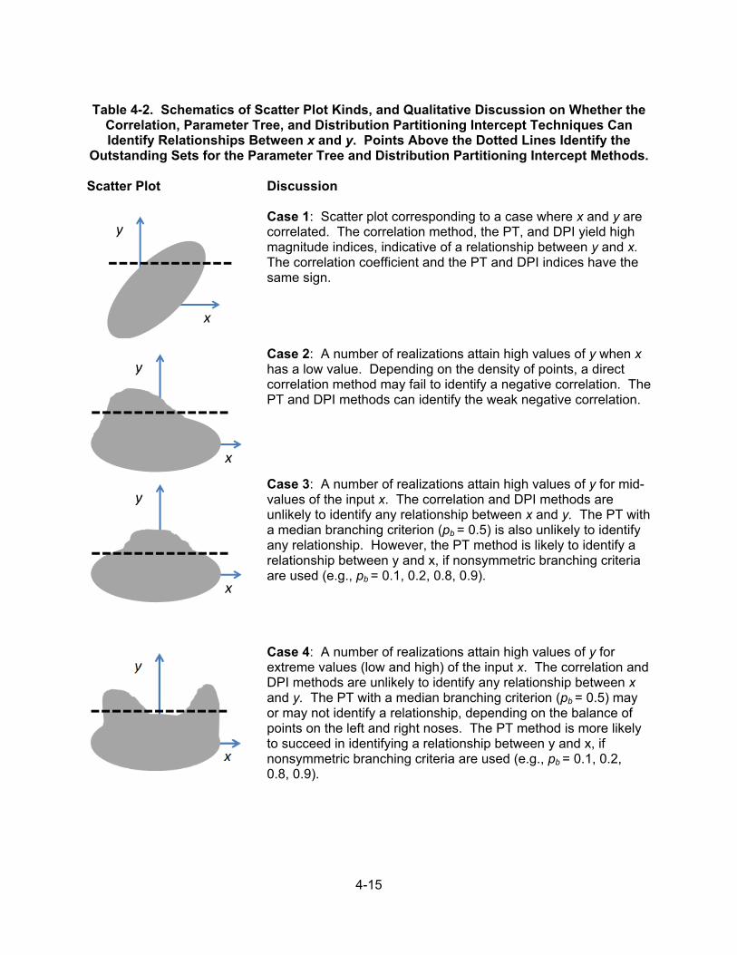
4-15

Table 4-2. Schematics of Scatter Plot Kinds, and Qualitative Discussion on Whether the

Correlation, Parameter Tree, and Distribution Partitioning Intercept Techniques Can Identify Relationships Between x and y. Points Above the Dotted Lines Identify the

Outstanding Sets for the Parameter Tree and Distribution Partitioning Intercept Methods.

Scatter Plot Discussion

Case 1: Scatter plot corresponding to a case where x and y are correlated. The correlation method, the PT, and DPI yield high magnitude indices, indicative of a relationship between y and x. The correlation coefficient and the PT and DPI indices have the same sign.

Case 2: A number of realizations attain high values of y when x has a low value. Depending on the density of points, a direct correlation method may fail to identify a negative correlation. The PT and DPI methods can identify the weak negative correlation.

Case 3: A number of realizations attain high values of y for mid-values of the input x. The correlation and DPI methods are unlikely to identify any relationship between x and y. The PT with a median branching criterion (pb = 0.5) is also unlikely to identify any relationship. However, the PT method is likely to identify a relationship between y and x, if nonsymmetric branching criteria are used (e.g., pb = 0.1, 0.2, 0.8, 0.9).

Case 4: A number of realizations attain high values of y for extreme values (low and high) of the input x. The correlation and DPI methods are unlikely to identify any relationship between x and y. The PT with a median branching criterion (pb = 0.5) may or may not identify a relationship, depending on the balance of points on the left and right noses. The PT method is more likely to succeed in identifying a relationship between y and x, if nonsymmetric branching criteria are used (e.g., pb = 0.1, 0.2, 0.8, 0.9).

x

y

x

y

x

y

4-16

regulatory analyses where models are employed to examine and explain system compliance (or noncompliance) with prescribed regulatory standards. 4.5 Fractional Factorial Method

Factorial design has been used for physical experimentation (Box, 1961) and for testing computer codes and models (Andres, 2001). Factorial designs usually sample over a range of each parameter at fixed intervals (e.g., the 5th and 95th percentile for a 2-interval design or adding the 50th percentile for a 3-interval design). By sampling all parameters in a system in this manner, it is often possible to determine unambiguously the effects of the variations in a parameter and all combinations of parameters. A full-factorial design with M intervals requires MN samples, where N is the number of parameters being examined. However, when the number of parameters and intervals exceeds just a few, the number of experiments necessary quickly grows to an unreasonable value.

Fractional factorial methods require far fewer than MN experiments, but may produce ambiguous sensitivity results. For example, a so-called level-4 design for 330 sampled parameters and two intervals (5th and 95th percentiles of each parameter distribution) required 2,048 samples. Such a level-4 design can yield results for which the main effects of all parameters are distinct from each other and two-way interactions of other parameters, but can be confounded by some three-way and higher interactions of other parameters. Because many of the parameters in a PA involved models for which such interactions are likely, it is important to be able to distinguish true effects of parameters from confounding combinations of higher-order interactions. In many cases, it is possible to use other information generated in the runs to make this determination.

In general, the fractional factorial analysis was conducted in the following steps: (i) develop an initial fractional factorial design for all sampled parameters considering the largest number of runs that reasonably can be handled, (ii) from the results of the preliminary screening, perform an analysis of variance (ANOVA) to determine those parameters that appear significant at a specified confidence level, (iii) screen further the list of statistically significant parameters on the basis of information other than the ANOVA results, and (iv) repeat the analyses using a refined set of parameters and higher resolution designs until results are acceptably unambiguous.

For the example of the TPA Version 4.1 analysis, the initial screening employed a level-4 design for 330 parameters at 2 sampling intervals (5th and 95th percentiles), requiring 2,048 runs. The ANOVA on these results found that there were potentially 100 significant parameters of the 330 at the 95th percent confidence level for the 10,000-year time period of interest. These results were further screened to a list of 37 parameters by observations from other information generated in the simulations; for example, it was possible to eliminate all parameters related to seismic failure of the waste packages by observing independently that none of the waste packages failed by this mechanism and, therefore, that this was a spurious indication caused by higher order combinations of other parameters.

Using the reduced set of 37 parameters from the initial screening, another level-4 factorial design was set up requiring an additional 2,048 runs. With only 37 parameters, it was possible to observe 2- and 3-way interactions that were combinations of the main effects and to make inferences about the fourth- and higher order interactions of those parameters that might be explored by additional factorial designs. This reduced the list to only 8 potentially significant parameters, for which a full-factorial design could be constructed with only an additional

4-17

256 runs. From the final full-factorial design, it was possible to determine that there were 7 significant parameters for the 10,000-year case, and up to at least 6-way interactions among these parameters.

Results from the fractional factorial designs for the 10,000- and 100,000-year time periods of interest were similar to many of the other sensitivity results, although the ranking of the parameters often differed among the various techniques. The full-factorial results are also used to draw detailed tree diagrams that show explicitly the direct effect of the high and low parameters in combination on peak dose for the five most important parameters. Figure 4-10 illustrates a tree diagram from the 10,000-year time period of interest in the TPA Version 4.1 analysis. The path to the highest peak dose, 0.66 mrem/yr [0.0066 mSv], can be traced to the bottom right of the figure. Monte Carlo results using only the parameters identified by the fractional factorial designs indicate that most of the variance is indeed captured by the identified parameters. NRC staff concluded that the fractional factorial method is good at identifying sensitive parameters unambiguously if executed properly. It is also very useful for identifying clearly through ANOVA the interactions among the important parameters. Such interactions were not easily identified by the other sensitivity techniques used.

However, the fractional factorial results are not markedly better than those from other techniques NRC used to identify the most sensitive parameters individually. Among the disadvantages of the fractional factorial technique are (i) it still requires a large number of runs,

Figure 4-10. Tree Diagram From Factorial Design Results for 10,000-Year Simulation Period, TPA Version 4.1

4-18

especially if the number of chosen intervals is greater than 2; (ii) it requires a large investment in the analyst’s time to screen out possible confounding combinations of other parameters masquerading for the apparently sensitive parameter; and (iii) the runs required for the sensitivity analyses cannot be used directly to generate the desired uncertainty analysis results, such as the cumulative distribution of the peak doses or the mean dose.

4.6 Iterated Fractional Factorial Design

The Iterated Fractional Factorial Design (IFFD) technique is a statistical method based on fractional factorial methods, but is supposedly more efficient (Andres, 2001). It has been used in the Canadian repository efforts to identify a small number of influential parameters from among thousands used in their models with relatively few realizations.

The authors claim that the number of influential parameters cannot grow as fast as the total number of parameters, and that only a small number of parameters or parameter interactions contribute significantly to the variance in the results. The IFFD approach suggests grouping all parameters into a smaller number of groups instead of sampling the parameters individually. Then the group as a whole is sampled (i.e., each parameter in the group gets the same “p” value). Iterating the random groupings will identify the influential parameters as those that consistently appear in the most influential groups.

The authors provide a software package, SAM2WIN (described in the Appendix), that generates the parameter samples.

4.7 Parameter Tree and Distribution Partitioning Intercept Methods

4.7.1 Parameter Tree Method

Jarzemba and Sagar (2000) developed the parameter tree (PT) method as a technique to identify parameters that caused a performance metric (e.g., maximum dose for a realization) to attain high values. Pensado (2008) defined a sensitivity index based on a statistic to identify correlations between input parameters and outputs for a PA code. The general approach to compute the statistic and the sensitivity index is explained as follows.

Figure 4-11 displays a scatter plot of an output y versus an input x. The multiple points in the scatter plot represent multiple realizations of a stochastic model. A branching criterion, pb, to split the set of points with respect to the input x is selected. In this figure, the branching criterion selected is the median (pb = 0.5), represented by the solid vertical line passing through x = 0 (the median value in this example). The branching criterion pb can be any quantile. The next step is to identify the outstanding realizations with respect to the output y. For example, the outstanding set could be defined as the top 10 percent of realizations with respect to the magnitude of the output y. In Figure 4-11, the outstanding set, set O, is the set of points above the horizontal dotted line. The following symbols are adopted:

Set O – outstanding set, set of points above the dotted line Set L – set of points below the x-branching criterion (points to the left of the vertical line) Set U – set of points above the x-branching criterion (points to the right of the vertical line) N – Size(O), number of points in the outstanding set

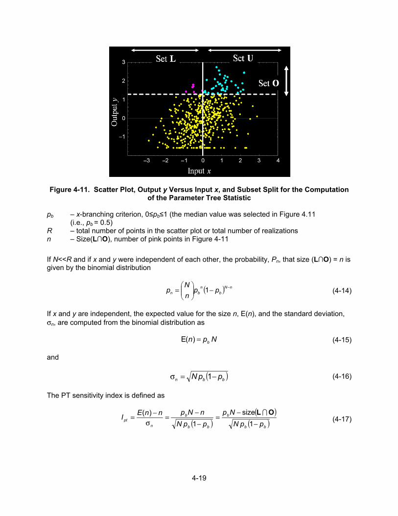
4-19

Figure 4-11. Scatter Plot, Output y Versus Input x, and Subset Split for the Computation of the Parameter Tree Statistic

pb – x-branching criterion, 0≤pb≤1 (the median value was selected in Figure 4.11

(i.e., pb = 0.5) R – total number of points in the scatter plot or total number of realizations n – Size(L∩O), number of pink points in Figure 4-11

If N<<R and if x and y were independent of each other, the probability, Pn, that size (L∩O) = n is given by the binomial distribution

( ) nN

b

n

bn ppn

Np −−

= 1

(4-14)

If x and y are independent, the expected value for the size n, E(n), and the standard deviation, σn, are computed from the binomial distribution as

Npn b=)(E (4-15)

and

( )bbn ppN −=σ 1

(4-16)

The PT sensitivity index is defined as

( )( )

( )bb

b

bb

b

n

ptppN

Np

ppN

nNpnnEI

−−

=−

−=

σ−=

1

size

1

)( OL

(4-17)

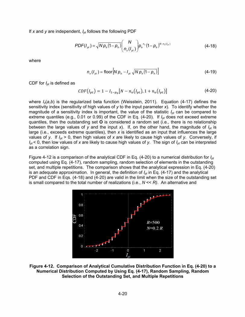
4-20

If x and y are independent, Ipt follows the following PDF

( ) ( ) )(1)(

1)( ptoo InN

b

n

bpto

bbpt ppIn

NppNIPDF −−

−=

(4-18)

where

( )[ ]bbptbpto ppNIpNIn −−= 1floor)( (4-19)

CDF for Ipt is defined as

1 , 1

(4-20)

where Iz(a,b) is the regularized beta function (Weisstein, 2011). Equation (4-17) defines the sensitivity index (sensitivity of high values of y to the input parameter x). To identify whether the magnitude of a sensitivity index is important, the value of the statistic Ipt can be compared to extreme quantiles (e.g., 0.01 or 0.99) of the CDF in Eq. (4-20). If Ipt does not exceed extreme quantiles, then the outstanding set O is considered a random set (i.e., there is no relationship between the large values of y and the input x). If, on the other hand, the magnitude of Ipt is large (i.e., exceeds extreme quantiles), then x is identified as an input that influences the large values of y. If Ipt > 0, then high values of x are likely to cause high values of y. Conversely, if Ipt < 0, then low values of x are likely to cause high values of y. The sign of Ipt can be interpreted as a correlation sign.

Figure 4-12 is a comparison of the analytical CDF in Eq. (4-20) to a numerical distribution for Ipt computed using Eq. (4-17), random sampling, random selection of elements in the outstanding set, and multiple repetitions. The comparison shows that the analytical expression in Eq. (4-20) is an adequate approximation. In general, the definition of Ipt in Eq. (4-17) and the analytical PDF and CDF in Eqs. (4-18) and (4-20) are valid in the limit when the size of the outstanding set is small compared to the total number of realizations (i.e., N << R). An alternative and

Figure 4-12. Comparison of Analytical Cumulative Distribution Function in Eq. (4-20) to a Numerical Distribution Computed by Using Eq. (4-17), Random Sampling, Random

Selection of the Outstanding Set, and Multiple Repetitions

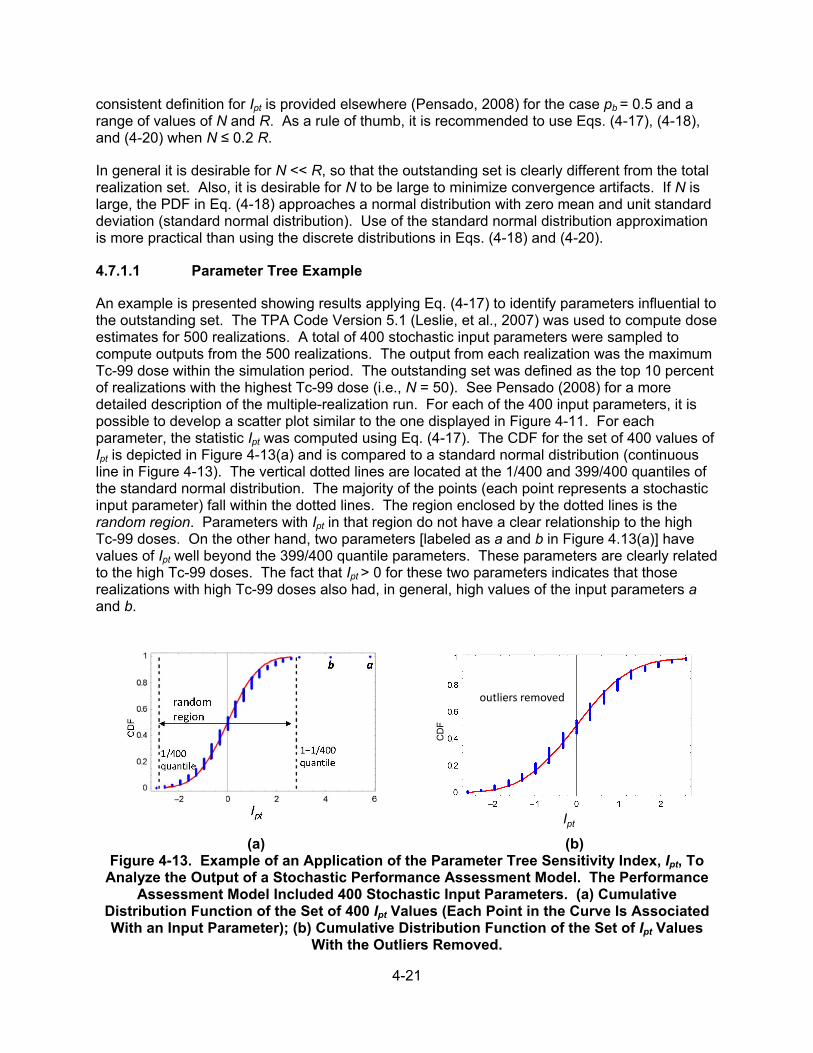
4-21

consistent definition for Ipt is provided elsewhere (Pensado, 2008) for the case pb = 0.5 and a range of values of N and R. As a rule of thumb, it is recommended to use Eqs. (4-17), (4-18), and (4-20) when N ≤ 0.2 R.

In general it is desirable for N << R, so that the outstanding set is clearly different from the total realization set. Also, it is desirable for N to be large to minimize convergence artifacts. If N is large, the PDF in Eq. (4-18) approaches a normal distribution with zero mean and unit standard deviation (standard normal distribution). Use of the standard normal distribution approximation is more practical than using the discrete distributions in Eqs. (4-18) and (4-20).

4.7.1.1 Parameter Tree Example

An example is presented showing results applying Eq. (4-17) to identify parameters influential to the outstanding set. The TPA Code Version 5.1 (Leslie, et al., 2007) was used to compute dose estimates for 500 realizations. A total of 400 stochastic input parameters were sampled to compute outputs from the 500 realizations. The output from each realization was the maximum Tc-99 dose within the simulation period. The outstanding set was defined as the top 10 percent of realizations with the highest Tc-99 dose (i.e., N = 50). See Pensado (2008) for a more detailed description of the multiple-realization run. For each of the 400 input parameters, it is possible to develop a scatter plot similar to the one displayed in Figure 4-11. For each parameter, the statistic Ipt was computed using Eq. (4-17). The CDF for the set of 400 values of Ipt is depicted in Figure 4-13(a) and is compared to a standard normal distribution (continuous line in Figure 4-13). The vertical dotted lines are located at the 1/400 and 399/400 quantiles of the standard normal distribution. The majority of the points (each point represents a stochastic input parameter) fall within the dotted lines. The region enclosed by the dotted lines is the random region. Parameters with Ipt in that region do not have a clear relationship to the high Tc-99 doses. On the other hand, two parameters [labeled as a and b in Figure 4.13(a)] have values of Ipt well beyond the 399/400 quantile parameters. These parameters are clearly related to the high Tc-99 doses. The fact that Ipt > 0 for these two parameters indicates that those realizations with high Tc-99 doses also had, in general, high values of the input parameters a and b.

(a) (b) Figure 4-13. Example of an Application of the Parameter Tree Sensitivity Index, Ipt, To

Analyze the Output of a Stochastic Performance Assessment Model. The Performance Assessment Model Included 400 Stochastic Input Parameters. (a) Cumulative

Distribution Function of the Set of 400 Ipt Values (Each Point in the Curve Is Associated With an Input Parameter); (b) Cumulative Distribution Function of the Set of Ipt Values

With the Outliers Removed.

outliers removed

Ipt

CD

F

4-22

Figure 4-13(b) includes the same points as Figure 4-13(a), but with the outliers (i.e., the points beyond, to the left and the right, the dotted lines) removed. This figure shows that the CDF for the set of Ipt for the stochastic input parameters can be reasonably compared to a standard normal distribution, as a practical approach to define hypothesis tests, and to discriminate parameters affecting high values of the model output from those that have a marginal or no effect.

4.7.2 Distribution Partitioning Intercept Method

The distribution partitioning intercept (DPI) method was designed as an extension of the PT method to define a sensitivity index as a statistic that would follow a continuous distribution (as opposed to the discrete distribution of the PT approach) (Pensado, 2008; Pensado and Sagar, 2004; Pensado, et al., 2002). The DPI method also relies on the outstanding set concept. The price to pay for the continuous distribution is a more complex method to compute the sensitivity statistic. On the other hand, the DPI method has the advantage that it does not need an arbitrary pb branching criterion. The approach to compute the sensitivity index is discussed as follows. Figure 4-4 is a scatter plot of output y versus the input x (same data as in Figure 4-11). As in Figure 4-11, the outstanding set, O, is the set of realizations with the top 10 percent values in the output y; depicted in Figure 4-14(a) as the set of points above the horizontal dotted line. Figure 4-14(b) shows the CDF of the input x, and the CCDF of the x values in the set O. The probability intercept of these curves is denoted as p. This probability intercept, p, is the statistic used to define the sensitivity index of the DPI method.

If the set O is random, N = size (O), N << R (R = number or realizations), and N is large enough, then the statistic p would follow a distribution described by (Pensado, 2008)

( )( )

33

12

21

)1(22)(

2

pp

eNpPDF

pp

pN

−π=

−−

−

(4-21)

The mean of Eq. (4-21) is 0.5. The standard deviation of p, σp, can be computed by numerical integration using the PDF in Eq. (4-21). Alternatively, the standard deviation can be approximated as (Pensado, 2008)

−≈σ

NNp

0923.025.0

1

(4-22)

The sensitivity index is defined as

−

−≈σ

−=

NN

ppEpI

p

dpi0923.0

25.01

5.0)(

(4-23)

4-23

(a) (b) Figure 4-14. (a) Scatter Plot, Output y Versus Input x, and Identification of the

Outstanding Set; (b) Computation of the p-Intercept Statistic as the Probability Intercept of the Input Parameter x Cumulative Distribution Function and the Set O Complementary

Cumulative Distribution Function

As a practical hypothesis test, a standard normal distribution can be used to discriminate significant magnitudes of Idpi. The sign of Idpi has a similar interpretation as the sign of Ipt: Idpi>0 implies that high values of the output are associated with high values of the input x. Conversely, Idpi < 0 implies that high values of the output are associated with low values of the input x.

4.7.2.1 Distribution Partitioning Intercept Example

This example uses the same data that were used to exercise the PT technique. See Pensado (2008) for details in the multiple-realization run of the PA model. The results are summarized in Figure 4-15. Figure 4-15(a) is a numerical CDF of the set of Idpi values associated with the 400 stochastic input parameters. Each point in Figure 4-15(a) is associated with one input parameter. The numerical CDF is compared to the CDF of a standard normal distribution (continuous line). The dotted vertical lines are located at the 1/400 and 399/400 quantiles of the standard normal distribution. The region between the dotted lines defines the random region. Parameters with an Idpi falling in this region are not significantly related to realizations with high magnitude output. There is only one parameter, labeled as a in Figure 4-15(a), that clearly has an outlier value of Idpi. Realizations with high value in the output tend to have a high value of the parameter a. The parameter a was also identified as significant using the PT index [see Figure 4-13(a)]. In Figure 4-13(b), the outliers were removed to enhance the comparison of the numerical CDF to the standard normal distribution CDF. Figure 4-13(b) shows that it is appropriate to use the standard normal distribution to define hypothesis tests.

4.7.3 Discussion

Both the PT and the DPI methods rely on the identification of a subset of realizations as the outstanding set (symbolized as O). The techniques determine whether there is something unique in set O about the input parameter x. If values of the parameter x are biased in the set O, both techniques can detect the bias, and identify x as an influential parameter if the bias is significant. Comparison of the magnitude of the index to a high quantile of the standard normal distribution is used to identify when an index is of high magnitude. Parameters with high magnitude indices are identified as likely influential to the output.

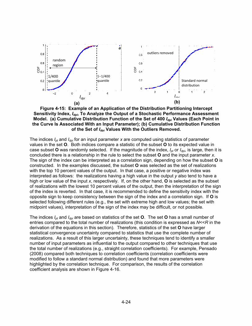
4-24

(a)

Figure 4-15: Example of an Application of the Distribution Partitioning Intercept Sensitivity Index, Idpi, To Analyze the Output of a Stochastic Performance Assessment Model. (a) Cumulative Distribution Function of the Set of 400 Idpi Values (Each Point in the Curve Is Associated With an Input Parameter); (b) Cumulative Distribution Function

of the Set of Idpi Values With the Outliers Removed.

The indices Ipt and Idpi for an input parameter x are computed using statistics of parameter values in the set O. Both indices compare a statistic of the subset O to its expected value in case subset O was randomly selected. If the magnitude of the index, Ipt or Idpi, is large, then it is concluded there is a relationship in the rule to select the subset O and the input parameter x. The sign of the index can be interpreted as a correlation sign, depending on how the subset O is constructed. In the examples discussed, the subset O was selected as the set of realizations with the top 10 percent values of the output. In that case, a positive or negative index was interpreted as follows: the realizations having a high value in the output y also tend to have a high or low value of the input x, respectively. If, on the other hand, O is selected as the subset of realizations with the lowest 10 percent values of the output, then the interpretation of the sign of the index is reverted. In that case, it is recommended to define the sensitivity index with the opposite sign to keep consistency between the sign of the index and a correlation sign. If O is selected following different rules (e.g., the set with extreme high and low values; the set with midpoint values), interpretation of the sign of the index may be difficult, or not possible.

The indices Ipt and Idpi are based on statistics of the set O. The set O has a small number of entries compared to the total number of realizations (this condition is expressed as N<<R in the derivation of the equations in this section). Therefore, statistics of the set O have larger statistical convergence uncertainty compared to statistics that use the complete number of realizations. As a result of this larger uncertainty, these techniques tend to identify a smaller number of input parameters as influential to the output compared to other techniques that use the total number of realizations (e.g., straight correlation coefficients). For example, Pensado (2008) compared both techniques to correlation coefficients (correlation coefficients were modified to follow a standard normal distribution) and found that more parameters were highlighted by the correlation technique. For comparison, the results of the correlation coefficient analysis are shown in Figure 4-16.

a

random region

1/400 quantile

1−1/400 quantile

Idpi

CD

F

Standard normal distribution

outliers removed

Idpi

CD

F

(b)

4-25

Figure 4-16. Identification of Influential Parameters to the Output Using a Technique

Based on Correlation Coefficients. There Are More Outliers Than Displayed in Figures 4-13 and 4-15.

The correlation sensitivity index, Ir, is defined as (Pensado, 2008)

21

2

r

RrIr

−

−=

(4-24)

where R is the total number of realizations and r is the traditional correlation coefficient between the input x and output y. Both the input and output data were rank transformed before the computation of the correlation coefficients (Pensado, 2008). If x and y are independent, the index Ir follows a standard normal distribution in the limit when R is large. This section concludes with a discussion of hypothetical situations under which the PT and DPI methods perform better than traditional methods such as correlation analysis. Table 4-2 includes scatter plot schematics for different hypothetical situations, without being exhaustive of the possibilities. The scatter plots are depicted as shadows, for the sake of simplicity. Table 4-2 shows a number of cases, such as a simple monotonic relationship between x and y (Case 1), non-monotonic relationships optimizing the output y in the midrange of the input (Cases 2, 3), or a non-monotonic relationship optimizing y in the extreme ranges (low or high values) of the input x (Case 4). Case 1 (or the negative correlation variant) is commonly detected by traditional sensitivity techniques. The other cases are difficult, in general, to be detected. If present, these relationships (Cases 2 to 4) tend to be less influential on the output than monotonic relationships; thus, the associated sensitivity indices tend to be masked by the higher magnitude indices associated with monotonic relationships between input and output. A number of physical situations could yield dependencies such as depicted in Table 4-2, Cases 2 to 4. In the PA there could be threshold parameters of conditions to be attained before other physical processes could be manifested. For example, a relationship between radionuclide leach rates from contaminated soil and infiltration rates may be established only after the soil is saturated with water. A system temperature may need to drop below a certain value, before water could contact an engineered barrier system (EBS) and carry radionuclides away. The water content in air (i.e., relative humidity) may need to attain certain high values before microbial action may affect corrosion and radionuclide transport. The balance between water infiltration rate and evaporation rates may lead to competing processes affecting

ab

random region

1/400 quantile

1−1/400 quantile

Rank transformed data

Ir

CD

F

4-26

corrosion of EBS materials. For example, if the water infiltration rate is too high, diluted waters may contact the EBS, which may not be corrosive. If the water infiltration rate is too low, the system may dry and EBS materials may not corrode. A balance between water infiltration and evaporation rates needs to be attained to lead to sustainable solutions causing corrosion of EBS materials. Scatter plots such as in Table 4-2, Cases 2 and 3 may indicate threshold or competing processes. An example of a physical process leading to a relationship as in Table 4-2, Case 4, is waste form dissolution. Waste forms may dissolve at high rates in solutions of low or high pH. A scatter plot of the release rate versus solution pH may have a similar shadow as in Case 4 in Table 4-2. Again, in the experience of the authors, input parameters leading to relationships to the output as depicted in Table 4-2, Cases 2 to 4 tend to be shadowed by parameters having a monotonic influence on the output (Case 1). In summary, the PT and DPI methods yield similar solutions when the branching criterion for the PT method is selected as pb = 0.5 (median value in the variate x). The DPI method yields a continuum range of Idpi values. On the other hand, the PT method yields discrete values of the index Ipt and the analysis requires selection of a branching criterion. The DPI method does not need a branching criterion, but the DPI index is computationally more expensive (more effort is needed to program the method in a computer algorithm, and it takes longer for the computer algorithm to run). The need to select a branching criterion in the PT method can be considered both a disadvantage and an advantage. It is a disadvantage because different results can be produced by the PT method depending on the branching criterion adopted, making the interpretation of the results more difficult. It is an advantage because flexibility in the branching criterion allows the identification of special relationships (see Table 4-2, Cases 3 and 4) that are overlooked by the DPI method. Given the preponderance of Case 1 (Table 4-2) relationships in PA models, correlation methods may identify the majority of influential parameters to an output. The disadvantage of correlation methods, on the other hand, is that results are dependent on changes of scale and transformations to the inputs and outputs [see Pensado (2008) for a more detailed discussion]. Thus, correlation methods and variants (e.g., multilinear regression, stepwise regression) have certain degree of subjectivity. On the other hand, the PT and DPI methods, being based on statistics in the probability range, yield results that are independent of changes of scale or transformations to inputs and outputs (Pensado, 2008).

4.8 Barrier Performance Evaluation by Signal Processing Techniques

Releases of radionuclides from the waste form would pass through several barriers such as the unsaturated zone (UZ) and saturated zone (SZ) before reaching the accessible environment. NRC staff developed an interesting technique to postprocess PA results from the Yucca Mountain Project in order to determine the effectiveness of intermediate barriers, comparing the rates of release from the EBS, UZ, and SZ for the long-lived radionuclides Np-237, Pu-242, and Tc-99. From insights derived in this study, it should be possible to determine the importance (and thus the sensitivity) of these barriers to overall performance. A direct approach for comparing the effectiveness of the UZ and SZ barriers uses methods for processing of digital signals, which require no accounting for the actual transport models involved.

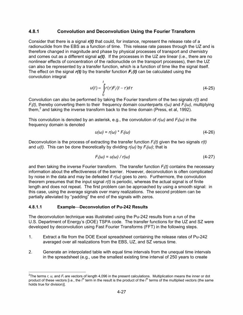
4-27

4.8.1 Convolution and Deconvolution Using the Fourier Transform

Consider that there is a signal r(t) that could, for instance, represent the release rate of a radionuclide from the EBS as a function of time. This release rate passes through the UZ and is therefore changed in magnitude and phase by physical processes of transport and chemistry and comes out as a different signal u(t). If the processes in the UZ are linear (i.e., there are no nonlinear effects of concentration of the radionuclide on the transport processes), then the UZ can also be represented by a transfer function, which is a function of time like the signal itself. The effect on the signal r(t) by the transfer function Fi (t) can be calculated using the convolution integral

−=t

i dtFrtu

0

)()()( τττ (4-25)

Convolution can also be performed by taking the Fourier transform of the two signals r(t) and Fi(t), thereby converting them to their frequency domain counterparts r(ω) and Fi(ω), multiplying them,2 and taking the inverse transform back to the time domain (Press, et al, 1992). This convolution is denoted by an asterisk, e.g., the convolution of r(ω) and Fi(ω) in the frequency domain is denoted

u(ω) = r(ω) * Fi(ω) (4-26)

Deconvolution is the process of extracting the transfer function Fi(t) given the two signals r(t) and u(t). This can be done theoretically by dividing r(ω) by Fi(ω); that is

Fi(ω) = u(ω) / r(ω) (4-27)

and then taking the inverse Fourier transform. The transfer function Fi(t) contains the necessary information about the effectiveness of the barrier. However, deconvolution is often complicated by noise in the data and may be defeated if r(ω) goes to zero. Furthermore, the convolution theorem presumes that the input signal r(t) is periodic, whereas the actual signal is of finite length and does not repeat. The first problem can be approached by using a smooth signal: in this case, using the average signals over many realizations. The second problem can be partially alleviated by “padding” the end of the signals with zeros.

4.8.1.1 Example⎯Deconvolution of Pu-242 Results

The deconvolution technique was illustrated using the Pu-242 results from a run of the U.S. Department of Energy’s (DOE) TSPA code. The transfer functions for the UZ and SZ were developed by deconvolution using Fast Fourier Transforms (FFT) in the following steps. 1. Extract a file from the DOE Excel spreadsheet containing the release rates of Pu-242

averaged over all realizations from the EBS, UZ, and SZ versus time.

2. Generate an interpolated table with equal time intervals from the unequal time intervals in the spreadsheet (e.g., use the smallest existing time interval of 250 years to create

2The terms r, u, and Fi are vectors of length 4,096 in the present calculations. Multiplication means the inner or dot product of these vectors [i.e., the ith term in the result is the product of the ith terms of the multiplied vectors (the same holds true for division)].

4-28

a table with 4,000 timesteps in it). This equal timestepping was necessary for the FFT procedure.

3. Because the FFT procedure requires that the number of discrete intervals be an

exponential factor of 2, “pad” the signals with 96 zeros added to the end of each column for the EBS, UZ, and SZ. This creates a data table of 4,096 (i.e., 212) rows. Padding also minimizes the effects of the nonperiodic nature of the signals.

4. Generate the frequency domain functions for the release rate for each radionuclide from

the EBS, the UZ, and the SZ using the FFT.

5. Calculate the frequency domain transfer functions of the UZ and SZ for each radionuclide using Eq. (4-27) (e.g., the transfer function in the frequency domain for the UZ would be simply the FFT of the UZ output divided by the FFT of the EBS output).

6. Generate the time domain transfer function for the UZ and SZ for each radionuclide using the inverse FFT.

Figure 4-17 shows the Pu-242 transfer function for the UZ as a function of timestep, each of which is 250 years. The FFT algorithm uses steps rather than actual time. The shape of the transfer function is essentially an impulse or δ function, which indicates that on the million-year timeframe of interest, there is virtually no effect of a time delay between the EBS and UZ releases, and that the releases would be diminished by a constant factor of 0.6615 by the UZ.3 That is, nearly all of the information about the transfer function is contained in the first timestep, and it has a value of 0.6615. This was a surprising conclusion, but it nevertheless appears to be correct, as shown in Figure 4-18. The release rate from the UZ can be closely predicted by simply multiplying the release from the EBS by a factor of 0.6615. Therefore, time delay through the UZ plays no significant role in the results, at least for the data analyzed, which is an average of 300 realizations. Figure 4-19 shows the Pu-242 transfer function for the SZ as a function of timestep. The shape is similar to that of the UZ in that there is no apparent effect of a time delay in the SZ, but the releases from the UZ would be diminished by a factor of about 0.354. Therefore, for the case of Pu-242, the SZ appears to reduce the releases to the accessible environment more effectively than the UZ. In contrast to Pu-242, the radionuclide Tc-99 is only slightly retarded, if at all. The same procedures were followed for releases of Tc-99 from the EBS, UZ, and SZ to generate transfer functions for the UZ and SZ. The results are quite different from the highly retarded plutonium. As with the Pu-242 results, there is no apparent effect of a time delay in the million-year timeframe for Tc-99, and all necessary information is contained in the first timestep of the transfer function. The release of Tc-99 would be diminished by the UZ by

3The convolution of a function of time f(t) with the δ function is just the value of the function at the time the δ function

occurs [ i.e., ∞

∞−

=− )()()( 00 tfdttttf δ (Wylie, 1982)]. The transfer functions in Figures 4-17 and 4-19 are not

strictly δ functions, because they are finite, but the area under the functions are constants (0.6615 and 0.345, respectively). For the purposes here, they can be considered to be δ functions at t = 0.

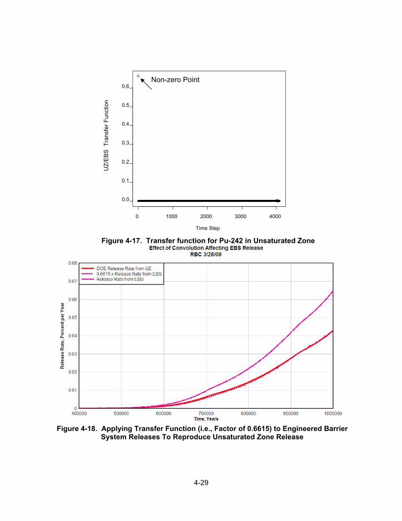
4-29

Figure 4-17. Transfer function for Pu-242 in Unsaturated Zone

Figure 4-18. Applying Transfer Function (i.e., Factor of 0.6615) to Engineered Barrier System Releases To Reproduce Unsaturated Zone Release

0 1000 2000 3000 4000

0.0

0.1

0.2

0.3

0.4

0.5

0.6

Time Step

Non-zero Point

UZ

/EB

S

Tra

nsfe

r F

unct

ion

4-30

Figure 4-19. Transfer Function for Release of Pu-242 in Saturated Zone a factor of about 0.963. However, there is no apparent diminishment of Tc-99 by the SZ (transfer function = 1.003). Therefore, the UZ appears to be more effective than the SZ for Tc-99 and probably for other nonretarded dissolved radionuclides like Cl-36 and perhaps Np-237.

4.8.2 Conclusions

Digital signal processing indicates that transport for both the UZ and SZ also can be successfully represented by a simple scaling factor. Results based on the DOE average of 300 realizations indicate that transport through the SZ was more effective than the UZ for highly retarded and/or filtered Pu-242. In the case of Tc-99, which is not expected to be highly retarded or filtered, the UZ appears to be more effective. However, the amount of removal of Tc-99 in either the UZ or SZ would be small. All of these analyses were conducted on results of the TSPA models that were averaged over 300 realizations. However, the deconvolution method did not work well on individual realizations because of the noisiness of the signals.

4.9 Component Sensitivity Analysis

Risk assessment models for large, complex systems are simplified representations that embody physical features and simulate many coupled processes with uncertainties. Model sensitivity analyses can be used to identify system attributes contributing most to risk. A measure of sensitivity is the change in model behavior caused by potential changes in model attributes. All model attributes cannot be simplified to the same degree in a model. Therefore, several different types of sensitivity analyses may be needed to adequately and consistently identify factors driving system risk/performance. One such method, referred to as the component sensitivity analysis method, was an analytical approach for estimating the sensitivity of a model of a complex system to changes in a subsystem or a component of that system. In this method, the component or subsystem is an element of the system with some performance value. Component sensitivity is the system response sensitivity to change in component functionality. This sensitivity is computed by using two cases the basecase and the

0 1000 2000 3000 4000

0.00

0.05

0.10

0.15

0.20

0.25

0.30

0.35

Time Step

Non-zero Point

SZ

/UZ

Tra

nsfe

r F

unct

ion

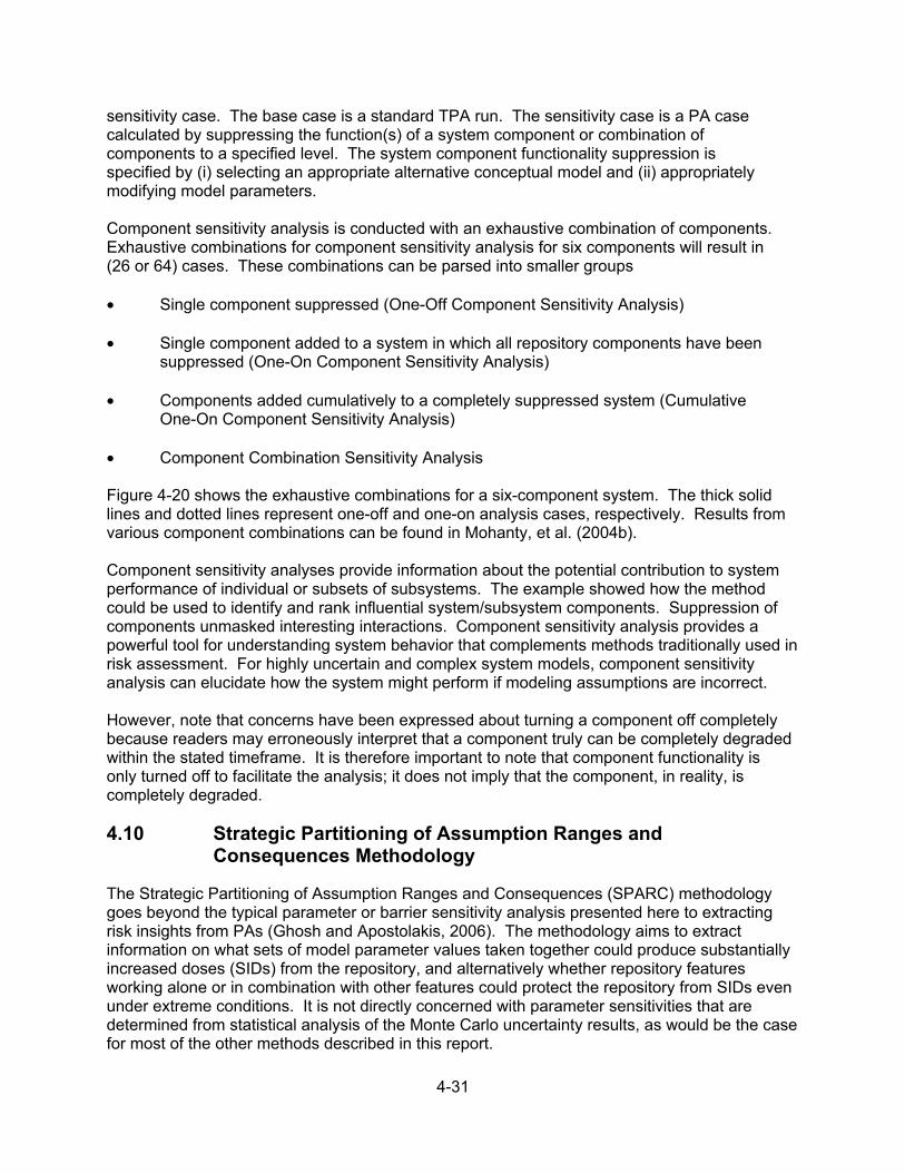
4-31

sensitivity case. The base case is a standard TPA run. The sensitivity case is a PA case calculated by suppressing the function(s) of a system component or combination of components to a specified level. The system component functionality suppression is specified by (i) selecting an appropriate alternative conceptual model and (ii) appropriately modifying model parameters. Component sensitivity analysis is conducted with an exhaustive combination of components. Exhaustive combinations for component sensitivity analysis for six components will result in (26 or 64) cases. These combinations can be parsed into smaller groups • Single component suppressed (One-Off Component Sensitivity Analysis)

• Single component added to a system in which all repository components have been

suppressed (One-On Component Sensitivity Analysis)

• Components added cumulatively to a completely suppressed system (Cumulative One-On Component Sensitivity Analysis)

• Component Combination Sensitivity Analysis

Figure 4-20 shows the exhaustive combinations for a six-component system. The thick solid lines and dotted lines represent one-off and one-on analysis cases, respectively. Results from various component combinations can be found in Mohanty, et al. (2004b). Component sensitivity analyses provide information about the potential contribution to system performance of individual or subsets of subsystems. The example showed how the method could be used to identify and rank influential system/subsystem components. Suppression of components unmasked interesting interactions. Component sensitivity analysis provides a powerful tool for understanding system behavior that complements methods traditionally used in risk assessment. For highly uncertain and complex system models, component sensitivity analysis can elucidate how the system might perform if modeling assumptions are incorrect. However, note that concerns have been expressed about turning a component off completely because readers may erroneously interpret that a component truly can be completely degraded within the stated timeframe. It is therefore important to note that component functionality is only turned off to facilitate the analysis; it does not imply that the component, in reality, is completely degraded.

4.10 Strategic Partitioning of Assumption Ranges and Consequences Methodology

The Strategic Partitioning of Assumption Ranges and Consequences (SPARC) methodology goes beyond the typical parameter or barrier sensitivity analysis presented here to extracting risk insights from PAs (Ghosh and Apostolakis, 2006). The methodology aims to extract information on what sets of model parameter values taken together could produce substantially increased doses (SIDs) from the repository, and alternatively whether repository features working alone or in combination with other features could protect the repository from SIDs even under extreme conditions. It is not directly concerned with parameter sensitivities that are determined from statistical analysis of the Monte Carlo uncertainty results, as would be the case for most of the other methods described in this report.

4-32

Figure 4-20. Exhaustive Combinations of Component Sensitivity Analysis Cases for Six Components in the Example Problem. Columns A and B Represent Sensitivities With

Respect to the Basecase and the Fully Suppressed Case, Respectively. The Thick Solid Lines and Dotted Lines Represent One-Off and One-On Analysis Cases, Respectively. (Acronyms: Dash—Not Analyzed, DS—Drip Shield, WP—Waste Package, SF—Waste

Form, IV—Invert, UZ—Unsaturated Zone, SZ—Saturated Zone, 0–0 Percent Functional; 100–100 Percent Functional) (Mohanty, et al, 2004b, reprinted with kind permission from

Springer Science+Business Media, B.V.)

4-33

SPARC is based on principals and ideas of reactor probabilistic risk assessment (PRA). However, PRA-style fault trees, event trees, and scenarios cannot be applied directly for the HLW repositories because their system natures are very different. Some of the salient differences include the following: • Reactors are designed not to fail, whereas the repository system is expected to “fail”

(degraded performance) eventually, sometime in the distant future. • Most basic events in level-1 reactor PRAs are modeled as binary, random failures,

whereas repository components degrade in complex, continuous processes in which their performance declines slowly.

• For HLW repositories, there is no analogous end state to core damage for reactors,

which simply signifies that the reactor has failed to prevent an accident; core damage is a binary end state—the core is either damaged or not. “Failure” and “success” have to be redefined for repositories where the end state, projected doses to people living near the repository, has continuous possible values and no sharp binary distinction.

Because of the limitations of reactor PRA as applied to repositories, the behavior of interest is based on delivery of a specified peak dose or greater to any individual affected by releases from the repository (i.e., SIDs.) An SID scenario is defined as a collection of features, events, and processes (FEPs) that leads to repository performance greater than a regulatory goal {e.g., 15 mrem/yr [0.15 mSv/yr] to the Reasonably Maximally Exposed Individual}. The SPARC methodology relies on the peak doses from individual realizations rather than the peak-of-the mean dose, which would be the basis on which regulatory compliance normally would be assessed. In this respect, a SID is not, by itself, a violation of the regulatory standard, which in most cases is based on the mean dose curve rather than a peak dose from an extreme realization of the PA model. In practice, the SID scenarios are defined in terms of combinations of sampled parameter intervals leading to SIDs. Figure 4-21 shows a conceptual representation of a scenario constructed as a combination of the parameter values in the shaded intervals of the PDFs. The goal of the SPARC method is to construct a specific explanation of the PA results of interest, which is needed for risk-informed decision making and risk-informing stakeholder deliberation. This includes information about how the repository may produce SIDs, even if the probability is very low, because a demonstration of low probability can add to the safety case. With the typical sampling algorithms such as LHS, these low-probability scenarios may not emerge from the Monte Carlo simulations because they are far out on the tail of the system level performance distribution. Better estimates of the distribution tail are needed to determine high-consequence/low-probability outcomes. Therefore, the goal is to find and/or construct SID scenarios that show specifically how the repository may result in SIDs, help identify dominant risk contributors, and serve as the basis for further model uncertainty studies.

4-34

Figure 4-21. A Scenario Defined as a Collection of Intervals of Performance Assessment Parameter Distributions (Ghosh and Apostolakis, 2006, Copyright 2006, by the American

Nuclear Society, La Grange Park, Illinois) 4.10.1 Steps in Strategic Partitioning of Assumption Ranges and Consequences Methodology 1. Screen Monte Carlo realizations to find important repository attributes⎯Before

there is a formal analysis, the analyst must first prescreen the safety case to estimate the likely reasons that the repository might produce SIDs. This involves identifying radionuclides that have adverse combinations of features (quantity, half-life, retardation, dose factors) and pathways that are most vulnerable. Following this screening, the SPARC methodology relies on initially determining peak dose results from Monte Carlo simulations of the PA model, as is the normal course of many other sensitivity and uncertainty analyses. Results are screened to identify the largest peak doses from the realizations and whether they exceed the regulatory limit (i.e., SIDs. The results are separated into those realizations that produce SIDs and those that produce doses below the regulatory limit.

2. Find SIDS scenarios⎯The next step is to compare the CDF of the distribution of each

sampled parameter corresponding to SID and non-SID categories to determine (i) whether they are drawn from the same or different distributions and (ii) whether there is any threshold for the sampled parameter, below which there are no SIDs. This part of the procedure uses “Generalized Sensitivity Analysis” (Hornberger and Spear, 1981). Figure 4-22 shows the presentation of the SID and non-SID CDFs for one parameter, WPFlowMF. This figure demonstrates: (i) the two CDFs are distinctly different, and

4-35

Figure 4-22. Cumulative Distribution Functions for Substantially Increased Doses and

Nonsubstantially Increased Dose Realizations for Parameter WPFlowMF (Ghosh and Apostolakis, 2006, Copyright 2006, by the American Nuclear Society,

La Grange Park, Illinois) therefore the parameter is likely to be significant (this can be determined from the K-S statistics if necessary) and (ii) there are no SIDs for WPFlowMF less than about 10. The second step of the analysis starts with the initial identification of SID scenarios from the Monte Carlo simulation. Parameters corresponding to the highest peak-dose realizations help to identify the likely intervals that would lead to SIDs. Then further Monte Carlo realizations can be computed, using ranges of the sampled parameters confined to those likely intervals rather than the entire range of the parameters.

3. Identify “Savior” Attributes⎯Savior attributes are parameters that would eliminate

SIDs, even under adverse scenarios. An intuitive example of a savior parameter identified this way is the failure time for the drip shield, because there could be no release prior to this failure. Another, less obvious example can be deduced from Figure 4-22, which suggests that there would be no SIDs for the parameter WPFlowMF below about 10. The SPARC method attempts to find savior parameters by sampling the identified sensitive parameters in narrow ranges confined to the likely intervals for SIDs, but sampling the remaining parameters over their normal ranges. Screening realizations are used to first find which parameter could explain best the successful realizations out of the whole set and then removing the realizations saved by this parameter. Successive screening then finds which parameter could best explain the successes in the remaining set of realizations and removing those realizations explained by it, and so on, until single parameters could no longer explain the success/SIDs divide in the remaining realizations. When it is no longer possible to identify single parameters with savior attributes, then it is possible to search for combinations of two or more parameters that serve that function. Figure 4-23 shows a plot of SIDs versus non-SIDs for values of two parameters, AAMAI@s and SAW%. This plot indicates that there are no SIDs in the lower left

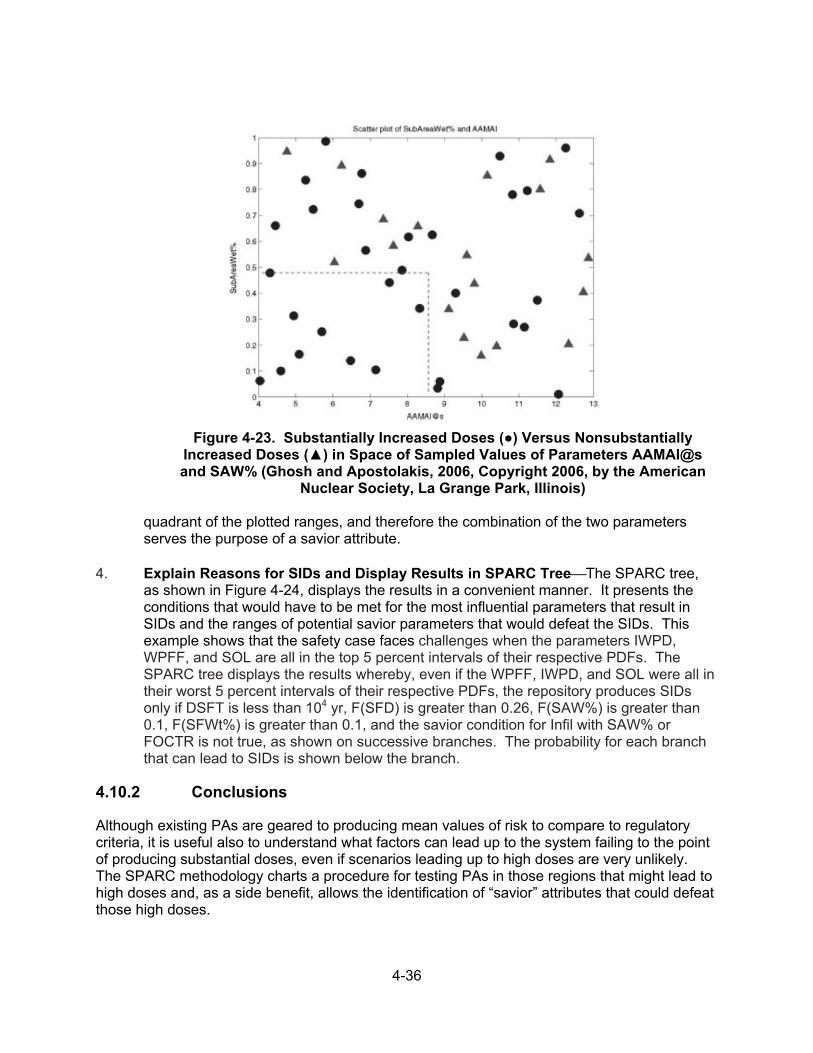
4-36

Figure 4-23. Substantially Increased Doses (●) Versus Nonsubstantially

Increased Doses (▲) in Space of Sampled Values of Parameters AAMAI@s and SAW% (Ghosh and Apostolakis, 2006, Copyright 2006, by the American

Nuclear Society, La Grange Park, Illinois) quadrant of the plotted ranges, and therefore the combination of the two parameters serves the purpose of a savior attribute.

4. Explain Reasons for SIDs and Display Results in SPARC Tree⎯The SPARC tree,

as shown in Figure 4-24, displays the results in a convenient manner. It presents the conditions that would have to be met for the most influential parameters that result in SIDs and the ranges of potential savior parameters that would defeat the SIDs. This example shows that the safety case faces challenges when the parameters IWPD, WPFF, and SOL are all in the top 5 percent intervals of their respective PDFs. The SPARC tree displays the results whereby, even if the WPFF, IWPD, and SOL were all in their worst 5 percent intervals of their respective PDFs, the repository produces SIDs only if DSFT is less than 104 yr, F(SFD) is greater than 0.26, F(SAW%) is greater than 0.1, F(SFWt%) is greater than 0.1, and the savior condition for Infil with SAW% or FOCTR is not true, as shown on successive branches. The probability for each branch that can lead to SIDs is shown below the branch.

4.10.2 Conclusions

Although existing PAs are geared to producing mean values of risk to compare to regulatory criteria, it is useful also to understand what factors can lead up to the system failing to the point of producing substantial doses, even if scenarios leading up to high doses are very unlikely. The SPARC methodology charts a procedure for testing PAs in those regions that might lead to high doses and, as a side benefit, allows the identification of “savior” attributes that could defeat those high doses.

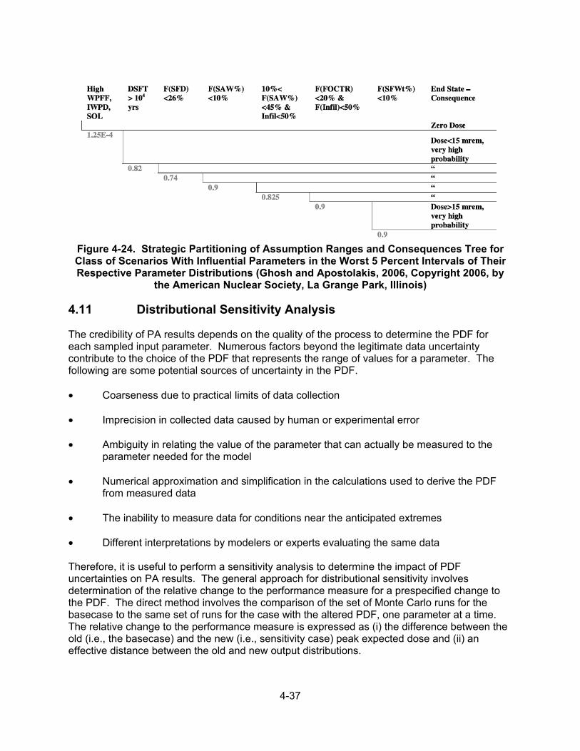
4-37

Figure 4-24. Strategic Partitioning of Assumption Ranges and Consequences Tree for Class of Scenarios With Influential Parameters in the Worst 5 Percent Intervals of Their Respective Parameter Distributions (Ghosh and Apostolakis, 2006, Copyright 2006, by

the American Nuclear Society, La Grange Park, Illinois)

4.11 Distributional Sensitivity Analysis The credibility of PA results depends on the quality of the process to determine the PDF for each sampled input parameter. Numerous factors beyond the legitimate data uncertainty contribute to the choice of the PDF that represents the range of values for a parameter. The following are some potential sources of uncertainty in the PDF.

• Coarseness due to practical limits of data collection

• Imprecision in collected data caused by human or experimental error • Ambiguity in relating the value of the parameter that can actually be measured to the

parameter needed for the model • Numerical approximation and simplification in the calculations used to derive the PDF

from measured data • The inability to measure data for conditions near the anticipated extremes

• Different interpretations by modelers or experts evaluating the same data

Therefore, it is useful to perform a sensitivity analysis to determine the impact of PDF uncertainties on PA results. The general approach for distributional sensitivity involves determination of the relative change to the performance measure for a prespecified change to the PDF. The direct method involves the comparison of the set of Monte Carlo runs for the basecase to the same set of runs for the case with the altered PDF, one parameter at a time. The relative change to the performance measure is expressed as (i) the difference between the old (i.e., the basecase) and the new (i.e., sensitivity case) peak expected dose and (ii) an effective distance between the old and new output distributions.

4-38

Studies of distributional sensitivity were carried out by the NRC and CNWRA staffs. The sensitivity cases were created by altering the PDF in one of three ways: (i) holding the mean constant, but changing the variance; (ii) shifting the mean, but holding the variance constant; or (iii) changing the mean while keeping the end points fixed. In the first two options, the basic shape of the PDF does not change. For the third option, however, the shape of the distribution will change. Figure 4-25 illustrates the third option for which the mean was shifted to the right by 10 percent while keeping the minimum and maximum values fixed. The shifted PDF is asymmetrical, unlike the symmetrical normal PDF from which it was derived. Details of the method, the results, and their interpretations can be found in Mohanty, et al. (2004a).

Figure 4-25. Example of (a) Changing the Probability Density Function for an Input

Parameter by Shifting the Mean Value of a Normal Distribution Function Without Changing the End Points and (b) the Corresponding Changes to the Cumulative

Distribution Functions (Mohanty, et al., 2004a)

5-1

5 INTERPRETING SENSITIVITY RESULTS 5.1 Introduction

Sensitivity results derived from the various techniques must be interpreted carefully because different methods often yield different results in terms of parameter sensitivity. The reasons for the differences in results must be understood and a consensus formed from the varying results to benefit the overall modeling objectives.

The remaining sections of this chapter will discuss the following aspects of sensitivity results:

• Collating parameter sensitivity results from different methods • Verification that sensitive parameters have been identified • Effect of using peak doses from each realization to calculate sensitivities • Effect of model conservatism on sensitivities

5.2 Collating Parameter Sensitivity Results From Multiple Methods

An important observation about parameter sensitivity methods is that they often give different evaluations of the sensitivities on the same data. Often, it is not clear at the beginning why these sensitivity evaluations give different results and which sensitivity methods are superior in performance. It is beneficial to include questionable parameters rather than taking the chance of missing an influential parameter at early stages of the sensitivity analysis. Moreover, at the early stages of performance assessments (PA), the impact of various parameters is less understood. At that stage, it is valuable to include a variety of sensitivity analysis methods to identify as many influential parameters as possible, even if some of the sensitivities are spurious.

The final list of sensitive parameters can be selected on the basis of how frequently they appear in all methods and on their importance rank by each method. The U.S. Nuclear Regulatory Commission (NRC) and the Center for Nuclear Waste Regulatory Analyses (CNWRA®) staff developed a heuristic method of assigning scores to the sensitive parameters. For TPA Version 4.1, the determination was done in two stages. The first stage combined the results for six statistical tests:

• Kolmogorov-Smirnov (K-S) + Sign Test—the rank of parameters that passed both the K-S and Sign tests.

• T-Norm—The rank of the t-value of a single-parameter regression of the normalized

parameters greater than 1.96 (95 percent confidence level).

• T-Rank—The rank of the t-value of a single-variable regression of the rank-transformed variables greater than 1.96 (95 percent confidence level).

• Step Raw—The rank of the variables from stepwise regression of the

normalized variables. • Step Rank—The rank of the variables from stepwise regression of the ranks of

the variables.Step Lnorm—The rank of the variables from stepwise regression of the log of the normalized variables.

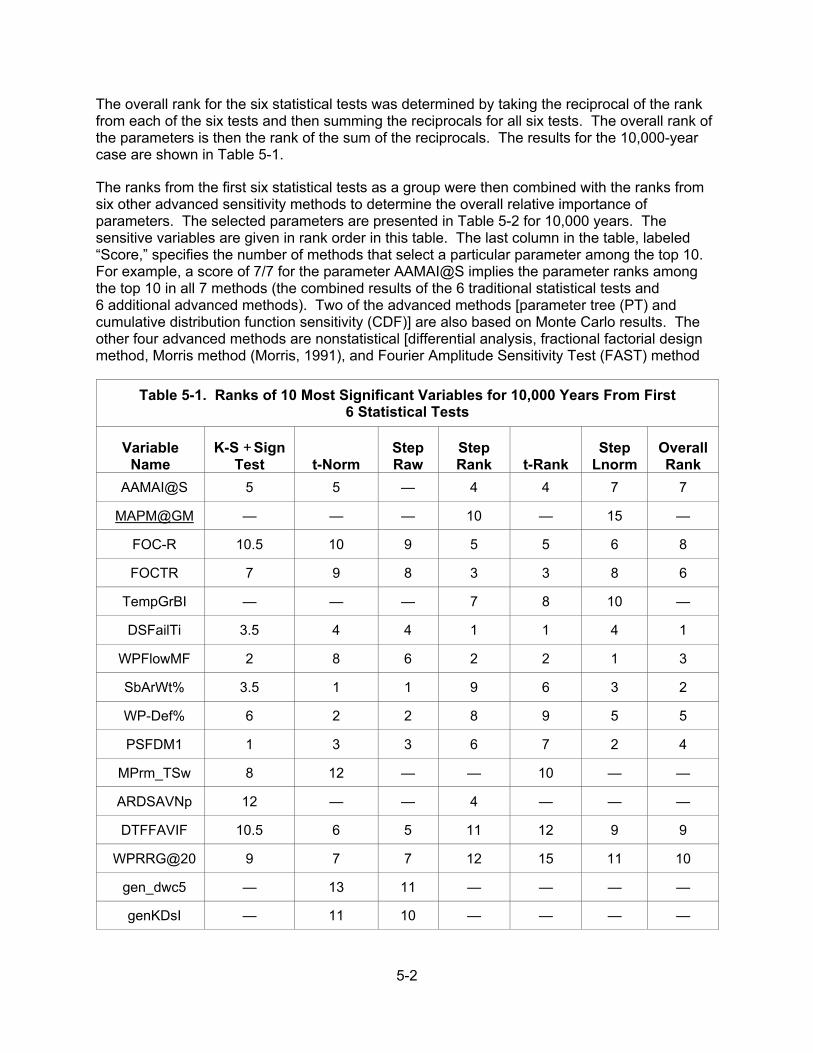
5-2

The overall rank for the six statistical tests was determined by taking the reciprocal of the rank from each of the six tests and then summing the reciprocals for all six tests. The overall rank of the parameters is then the rank of the sum of the reciprocals. The results for the 10,000-year case are shown in Table 5-1.

The ranks from the first six statistical tests as a group were then combined with the ranks from six other advanced sensitivity methods to determine the overall relative importance of parameters. The selected parameters are presented in Table 5-2 for 10,000 years. The sensitive variables are given in rank order in this table. The last column in the table, labeled “Score,” specifies the number of methods that select a particular parameter among the top 10. For example, a score of 7/7 for the parameter AAMAI@S implies the parameter ranks among the top 10 in all 7 methods (the combined results of the 6 traditional statistical tests and 6 additional advanced methods). Two of the advanced methods [parameter tree (PT) and cumulative distribution function sensitivity (CDF)] are also based on Monte Carlo results. The other four advanced methods are nonstatistical [differential analysis, fractional factorial design method, Morris method (Morris, 1991), and Fourier Amplitude Sensitivity Test (FAST) method

Table 5-1. Ranks of 10 Most Significant Variables for 10,000 Years From First 6 Statistical Tests

Variable Name

K-S + Sign Test t-Norm

Step Raw

Step Rank t-Rank

Step Lnorm

OverallRank

AAMAI@S 5 5 — 4 4 7 7

MAPM@GM — — — 10 — 15 —

FOC-R 10.5 10 9 5 5 6 8

FOCTR 7 9 8 3 3 8 6

TempGrBI — — — 7 8 10 —

DSFailTi 3.5 4 4 1 1 4 1

WPFlowMF 2 8 6 2 2 1 3

SbArWt% 3.5 1 1 9 6 3 2

WP-Def% 6 2 2 8 9 5 5

PSFDM1 1 3 3 6 7 2 4

MPrm_TSw 8 12 — — 10 — —

ARDSAVNp 12 — — 4 — — —

DTFFAVIF 10.5 6 5 11 12 9 9

WPRRG@20 9 7 7 12 15 11 10

gen_dwc5 — 13 11 — — — —

genKDsI — 11 10 — — — —

5-3

Table 5-2. Influential Parameters for the 10,000-Year Simulation Period From Sensitivity Analysis Studies

No.

Parameter Abbreviation Parameter Name Score

1 AAMAI@S Areal average mean annual infiltration at start 7/7

2 DSFailTi Drip shield failure time 7/7 3 PSFDM1 Preexponential term for spent nuclear fuel dissolution

Model 2 6/7

4 SbArWt% Subarea wet fraction 6/7

5 WPFlowMF Waste package flow multiplication factor 6/7

6 WPRRG@20 Well pumping rate at 20-km [12.4-mi] receptor group 6/7

7 FOCTR Fraction of condensate toward repository 4/7

8 ARDSAVNp Alluvium Rd for Np-237 3/7

9 DTFFAVIF Distance to tuff–alluvium interface 3/7 10 WP-Def% Waste package initially defective fraction 3/7

(Cukier, et al., 1973)], for which the sampled parameters were determined specifically for the method rather than being sampled by Monte Carlo. Note that the FAST method selects only the most influential parameters of the top 20 listed in the peak dose column for the 10,000-year case. The parameters that do not make the final list include those selected as influential by only one or two of the seven methods. Although not described here, the Morris method and FAST method are described in Mohanty, et al. (2004a). In addition, a publicly available R-language routine “Sensitivity” (CRAN, 2011) implement the Morris and FAST methods.

5.3 Verification of Sensitivity Analysis Results

Because most of the sensitivity analysis methods neither guarantee that the parameters are influential nor establish a degree of influence, it is important to verify that the group of parameters identified by various methods is truly influential. Because the system response is most affected by the most influential parameters identified with the sensitivity analyses, it is intuitive that the variance of the system response will be significantly reduced if the input variances of the influential parameters are reduced.

There are three ways to demonstrate that the most influential parameters have been identified.

1. Repeat the PA runs holding all parameters at their mean value, except the identified influential parameters, which are sampled as usual.

2. Repeat the PA runs, holding the identified influential parameters at their mean values

while sampling the remaining parameters as usual. 3. Repeat the PA runs allowing all parameters to be sampled as usual, except the

identified sensitive parameters, which are held at their mean values one at a time.

For the first two demonstrations, the variance reduction for the group of influential parameters is shown as a change in the shape of a complementary cumulative distribution function (CCDF) constructed from the performance values (e.g., the peak dose from each realization). These results are then compared to the CCDF from the original “basecase”

5-4

PA calculation. If the identification of influential parameters was successful, then the CCDF for the first demonstration should be quite similar to the original CCDF. Furthermore, the CCDF for the second demonstration should show a decrease in the spread of peak dose values. Results for the TPA Version 4.1 demonstration for 10,000-year time period of interest are shown in Figure 5-1. Based on this figure, it appears the scoring method ranked the top parameters correctly.

For the calculations of the reduction in variance for individual influential parameters, each influential parameter was held fixed at its mean value while the remaining input parameters were sampled. The results of this analysis in terms of the change in the standard deviation of peak dose and the coefficient of variation (CV) (standard deviation divided by mean) are presented in Table 5-3. Results from this calculation are not as clear cut as the influence of the whole set of identified influential parameters on the CCDF. Freezing an influential parameter at its mean value usually, but not always, leads to a corresponding reduction in CV, but the response is weak and sometimes ambiguous. For example, freezing drip-shield failure time (DSFailTi) at its mean increases peak dose variability, although the CV decreases.

5.4 Top-Down Correlations

Iman and Conover (1987) published an interesting and useful method for situations where objects are ranked by multiple independent sources or methods (e.g., ranking of sensitivities by several different statistical tests). The method places most weight on agreements and disagreements for the most important parameters and less weight on agreements and disagreements for unimportant parameters.

Figure 5-1. Effect on Complementary Cumulative Distribution Function of Peak Doses of Identified Influential Parameters

5-5

Table 5-3. Changes in Variance for Holding Identified Influential Parameters at Their Mean Values Individually

Abbreviation Mean-of-Peak Doses

(mrem/yr)

Standard Deviation of Peak Doses (mrem/yr)

Coefficient of Variation (Unitless)

Basecase 4.24 × 10−5 1.32 × 10−4

3.12 AAMAI@S 4.23 × 10−5

1.38 × 10−4 3.26

MAPM@GM 4.28 × 10−5 1.37 × 10−4

3.19 DSFailTi 7.20 × 10−5

2.00 × 10−4 2.78

WPFlowMF 3.61 × 10−5 1.03 × 10−4

2.85 gen_PUSF 4.20 × 10−5

1.31 × 10−4 3.12

WPRRG@20 4.07 × 10−5 1.26 × 10−4

3.09 ARDSAVNp 4.00 × 10−5

1.28 × 10−4 3.10

IPPFSTFF 4.36 × 10−5 1.38 × 10−4

3.16 PSFDM1 2.57 × 10−5

6.90 × 10−5 2.68

SbArWt% 3.85 × 10−5 1.15 × 10−4

2.99

genlvirC 4.21 × 10−5 1.31 × 10−4

3.12 WP-Def% 4.02 × 10−5

1.19 × 10−4 2.97

MPrm_PPw 4.24 × 10−5 1.32 × 10−4

3.12 DTFFAVIF 4.02 × 10−5

1.30 × 10−4 3.28

FPrs_STF 4.25 × 10−5 1.30 × 10−4

3.06 SFWt%I2 4.30 × 10−5

1.33 × 10−4 3.09

InvMPerm 4.24 × 10−5 1.33 × 10−4

3.12 SFWt%I9 4.33 × 10−5

1.37 × 10−4 3.16

SFWt%I1 4.33 x 10−5 1.27 × 10−4

3.08

gen_ifi 3.95 × 10−5 1.27 × 10−4

3.23

The top-down correlation requires the “Savage” score S(h) for the variable ranked h by the sensitivity method

==

n

hjjhS /1)(

(5-1)

where n is the number of ranked variables. For example, the highest ranked variable would have a score of 1/1 + 1/2 + 1/3 ….+ 1/n. The second ranked variable would have a score of 1/2 + 1/3 + ……+ 1/n (Kleijnen and Helton, 1999).

The “concordance” between two methods, 1 and 2, is the correlation coefficient R12 associated with the pairs of the Savage scores for each variable

)]1(/[)()(1

2112 SnnhShSRn

iii −

−=

= (5-2)

5-6

where S(1) is the Savage score for h = 1. A large positive value for R12 indicates agreement between the two ranking methods for the most important parameters. The probability p that the rankings between the two sensitivity methods would be caused by random variations can be calculated by the following formula

)2/2(5.0)( 1212 −=>= nRerfcRRprobp (5-3)

Values of R12 and p are calculated for all pairs of sensitivity methods. A high correlation coefficient and low p for a pair of ranking methods indicate that the methods agree for the most importantly ranked parameters.

Top-down correlations are calculated by the program PATTRN (Shortencarier and Helton, 1999), described in the Appendix.

5.5 Effect of Using Peak Doses To Calculate Sensitivities

The choice of the peak-of-the-mean or the mean-of-the-peaks can affect sensitivity results. Generally, sensitivity analyses are conducted using peak doses, but the timing of the peak dose from each realization does not always align with the time at which the peak-of-the-mean dose occurs. Consider for example the results from a TPA 4.1 sensitivity analysis (Mohanty, et al., 2004a). A ranking of the most sensitive parameters shows a marked difference for at least one parameter, DSFailTi, which is the failure time of the drip shield, represented in this model as a random time, with no objective or mechanistic basis (i.e., an aleatory parameter1). As shown in Figure 5-2, this parameter is of relatively low importance using the sensitivity based on the dose corresponding to the peak-of-the-mean. As shown in Figure 5-3, however, the parameter is of high importance based on the peak doses for each individual realization. Parameters that change the timing of the peak dose, like DSFailTi or the time of a volcanic eruption, behave differently from other parameters that only change the magnitude of the dose.

5.6 Effect of Model Conservatism on Sensitivity Studies

In conducting sensitivity analysis, an important implicit assumption is that the model and the associated parameters representing the system are realistic (i.e., neither overly pessimistic nor optimistic). However, analysts often err on the side of safety by picking conservative PDFs. Such choices are unavoidable when modeling large and complex systems, such as a high-level radioactive waste (HLW) disposal system, when the systems have significant levels of uncertainty and the available data is limited . Conservative assumptions imply underestimating the performance of the system.

1Note however that there may be a mechanistic basis for drip shield failure time, and that therefore DSFailTi is probably best classified as a parameter with reducible or “epistemic” uncertainty. However, in TPA Version 4.1, no such mechanistic model was used. The time of volcanic eruption, however, is probably best classified as aleatory.

5-7

Figure 5-2. Sensitivity Using Doses for Each Realization at Time of Peak-of-the-Mean Dose

Figure 5-3. Sensitivity Using Peak Doses From Each Realization

5-8

A model can be conservative for a variety of reasons: • Analysts simplify assumptions because of

— Paucity of data — Complexity of the processes modeled — Early stage of modeling — Limited resources and time

• Analysts simplify the model without any specific attention to conservatism or realism.

• Simplifying assumptions may be deliberately biased toward conservatism. • A multidisciplinary system model may have different degrees of conservatism in its

components. It integrates multiple abstracted conceptual and mathematical models from analysts with different levels of expertise or subject-specific biases.

CNWRA staff conducted a systematic study with the objectives of (i) investigating the effect of conservatism on the ranking of influential parameters and (ii) illustrating the effects at various levels of conservatism using simple, nonlinear, stochastic examples.

This study was illustrated through three simple, nonlinear stochastic example problems on how the ranking of influential parameters changes with the level of assumed conservatism. Such changes could lead to erroneous conclusions that other parameters in the system model are more influential than those assumed to be conservative.

5.6.1 Approach

The following is a summary of the approach used:

• Specify uncertainty range for each parameter in the response function

• Compute sensitivity coefficients corresponding to each input parameter

• Change the range of the specific input parameter whose effect on conservatism is investigated by (i) keeping the conservative end of the distribution fixed and (ii) shifting the nonconservative end of the distribution toward conservative values (i.e., the mean shifts conservatively)

• Repeat the computation of sensitivity

The generation of the conservative case is detailed in Mohanty and Nes (2006). Effects of conservatism were explained using three examples: (i) a generic four-parameter function; (ii) radiation dose from drinking water, where model output is inversely proportional to the parameter of interest (e.g., distribution coefficient); and (iii) external radiation dose from a contaminated layer of soil. Model output is directly proportional to the parameter of interest (e.g., layer thickness). Mathematically, all three problems were represented via nonlinear and analytic functions, thus allowing analytical computation of sensitivity coefficients.

In one example, sensitivity changed nonlinearly with conservatism, implying that parameters previously not most influential can become most influential depending on the level of

5-9

conservatism. In the example problem for which there is an inverse relationship between the parameters of interest and model response, greatest sensitivity was observed at the nonconservative end of the parameter ranges.

Three examples were used to illustrate how conservatism in model parameters can influence the sensitivity based ranking of influential parameters. Results showed that the sensitivity of model output changes nonlinearly with the conservatism built into the model through the conservative assumptions for parameter values. This nonlinearity is a function of the structure of the performance function. Over the uncertainty range of a parameter, the model output sensitivity to the parameter could vary from being insensitive to highly sensitive depending on the level of conservatism assumed. The sensitivity based ranking of influential parameters can change non-monotonically with the assumed level of conservatism, depending on the model structure. Such dependence of the ranking of influential parameters on conservative assumptions could lead an analyst to conclude that other parameters are more influential. Because conservatism in safety analysis models with large uncertainties is unavoidable, analysts should evaluate the effects of the assumed degree of conservatism or the use alternative methods (e.g., component sensitivity analysis) to ensure that influential parameters are correctly identified.

5.7 Conclusions

Methods to determine parametric sensitivity often give conflicting results. NRC and CNWRA staffs developed a procedure to combine the sensitivity results from multiple methods to form a consensus of most sensitive parameters. This procedure was then used to generate a CDF of peak doses varying only the identified sensitive parameters while holding all others at their mean values. Alternatively, holding the identified sensitive parameters at their mean values while sampling all other parameters led to a large decrease in variance of the peak dose. These tests demonstrated that the consensus method reproduced the original CDF to a high degree of accuracy.

Sensitivity analysis has usually been performed using the peak doses from each realization. However, this does not usually align with the peak-of-the-mean dose. Comparing sensitivities using doses at the time that the peak-of-the-mean occurs can lead to different conclusions about the sensitivity of certain parameters, particularly those that influence the timing of the peak doses for each realization.

Conservatism can affect conclusions about the sensitivity of parameters. Results showed that the sensitivity of model output changes nonlinearly with the conservatism built into the model through the conservative assumptions for parameter values.

6-1

6 EARLIER ACTIVITIES ON WASTE-PACKAGE PROBABILISTIC PERFORMANCE ANALYSES

6.1 Introduction This chapter summarizes some of the early activities related to the uncertainty assessments for the high-level radioactive waste (HLW)-package performance conducted in the late 1980s through 1990s. To address the performances of waste package designs under uncertainty, four uncertainty evaluation methods (probability distribution approach, bounding approach, expert judgment, and sensitivity analysis) were identified as elements of a probability based framework that, without either diminishing or enhancing the input uncertainties, could provide quantitative measures for assessing waste package design performance. The methods also helped to identify critical inputs as a guide to reducing uncertainty. It should be noted however that this work was pursued prior to the issuance of the Yucca Mountain-specific regulations put forward in 10 CFR Part 63, and several key concepts in the rule current at the time (10 CFR Part 60) no longer apply. Among the various differences are subsystem performance requirements such as groundwater travel time and substantially complete containment (SCC) that are contrary to current policy. Although 10 CFR Part 60 is still part of the Federal code, it is unlikely that it would apply in its present form to any future U.S. repository for high-level radioactive waste. The analyses as summarized here include the examinations of the earlier waste containment in the context of the previous regulation. These analyses are included in this report for completeness and to provide pointers to references related to these analyses. Bearing in mind that the regulations in effect when the majority of this work was performed are no longer applicable, much of the technical analysis is still valuable. In general, the uncertainty and sensitivity assessment methods summarized in this chapter are comprehensive and are applicable to engineered barrier systems (EBS). 6.1.1 Background The specific portions of the rules in effect at the time regarding the waste package include 10 CFR 60.112, Overall System Performance Objective for the Geologic Repository After Permanent Closure and 10 CFR 60.113, Performance of Particular Barriers after Permanent Closure, which states the performance requirements for the EBS and the geologic setting. The rules at 10 CFR 60.113 specified that the EBS should provide SCC during the period when radiation and thermal conditions in the EBS are dominated by fission product decay, and any release of radionuclides from the EBS should be a gradual process that results in small fractional releases to the geologic setting over long times. Therefore, the EBS-related analyses revolved around SCC. Although the requirement for limited release from the EBS in the postcontainment period was stated in numerical terms, the coupled requirement for SCC during the containment period was thought to be ambiguous and subject to interpretation. Accordingly, clarification of the meaning of the containment requirement either by rulemaking or some other uncertainty reduction method was thought to be needed. From the performance assessment (PA) perspective, three factors were thought to contribute to the uncertainty in waste package performance: (i) the required service time (more than

6-2

300 years) specified in the regulation exceeded the times commonly required in engineering design; (ii) the number of waste packages was very large (about 20,000 to 80,000 were expected), which implied that a full-scale laboratory test was practically impossible; and (iii) the waste packages would be inaccessible for close performance monitoring during the majority of the service life. Therefore, reasonable assurance of the required long-term performance would require good scientific understanding of the physics, including potential failure modes, and should apply conservative but reasonable assumptions of the effects of time and the environment on a repository. To clarify and investigate the feasibility of quantifying the containment regulation, the feasibility of a potential rulemaking activity related to containment was examined and three background technical reports were developed to provide a common technical basis from which a rule could be developed, if appropriate. The first report presented the technical topics that should be considered in assessments of the long-term performance of the waste package (Manaktala and Interrante, 1990; Manaktala, et al., 1990). The second report identified methodologies for assessing how well the various technical considerations could be evaluated in the presence of known and, at times, unknown uncertainties (Wu, et al., 1991). On the basis of the information provided in the first two reports, the third report provided recommendations related to SCC of the HLW within the waste package (Nair and Tschoepe, 1990). This chapter, with a focus on the uncertainty issues and methods applicable to waste package PA, is based on the second report and related reports and papers published in the early 1990s. A significant portion of the chapter related to the improvements of the standard Monte Carlo approach for uncertainty and reliability assessment developed over the years. These improvements were particularly suitable for providing faster “what if” answers to different assumptions for general probabilistic PA. 6.2 Waste Package Performance Assessment 6.2.1 Introduction For convenience, a waste package was defined as the waste form (radioactive waste materials and any encapsulating or stabilizing matrix) and any containers, shielding, packing, and other absorbent materials immediately surrounding an individual waste container; the EBS was defined as the waste packages plus the underground facility. The regulation in force at the time (10 CRF Part 60) addressed the ability of all the waste packages within the EBS to contain the waste during the period when radiation and thermal conditions in the EBS are dominated by fission product decay. Accordingly, a failure was defined as loss of containment function caused by the interaction between environments and waste package degradation processes. Waste package failure could be more explicitly defined only when a proposed design had well-defined materials and geometries. The consequence of waste package failure was the availability of nuclear waste for transport to the geologic setting. However, the amount or rate of release was regulated in a separate requirement discussed in Manaktala and Interrante (1990), which presented the various technical considerations required to make a logical argument for satisfying containment requirements. The higher order classification of the technical considerations included environment, materials fabrication, degradation processes, and inspections and monitoring. These considerations, when

6-3

incorporated into a life prediction methodology for waste packages, could become the basis for exercising technical judgment on the long-term performance of the containment barriers. Sridhar, et al. (1991); Cragnolino, et al. (1994); and Wu et al. (1988) reported examples of technical considerations and analyses.

6.2.2 Waste Package Failure Modes and Uncertainties

To assess waste package performance, it was considered necessary to investigate all the possible failure modes and the scenarios associated with each failure mode. Standard risk analysis techniques, such as fault-trees and failure-modes-and-effects analysis, were used to define failure paths and consequences. Potential failure modes included corrosion, radiation damage, and force and/or temperature-induced deformation or fracture (e.g., by seismic force). Uncertainties in failure modes were recognized to arise from design parameters such as the selected material, geometry, strength, and location.

Waste package environments were defined as time-dependent physical or chemical conditions imposed either externally or internally on a waste package and having the potential for affecting the performance to the extent of causing a waste package failure. Major waste package environments known to impact the waste package performance included geochemical condition, thermal field, radiation field, fluid flow field, stress and seismic fields, and surrounding medium (rocks and other barriers).

The geochemistry defined environmental conditions that initiated and/or propagated material degradation processes such as corrosion. It was known that uncertainties in geochemical characteristics could depend strongly on long-term predictive models.

The thermal field around waste packages depended on the type and amount of nuclear waste. Uncertainties in predicting the thermal field were thought to be caused by the difficulty in characterizing the thermal properties of the surrounding medium.

The radiation field could influence the characteristics of the surrounding materials and cause changes in the degradation rates. It was anticipated that the characteristics of the radiation field might have relatively smaller uncertainty; but that the radiation effect on the materials might have greater uncertainty which could be reduced only by physical understanding of the processes.

Fluid flow coupled with geochemical conditions could provide a mechanism for potentially corrosive chemicals to contact and degrade the waste packages. The locations and amount of water and vapor depended on many factors, such as climate, water table, and water flow characteristics of the rock matrix. It was expected that uncertainties might arise from long-term predictive models, such as those for recharge rates and groundwater flow.

The sources of stresses in a waste package were recognized to include those due to welding, sealing, and other fabrication processes and other mechanical forces imposed by, for example, the collapse of emplacement boreholes due to seismic shaking or fault motions caused by an earthquake. The stresses induced by seismic shaking and fault motions were subject to uncertainty.

The surrounding medium of a waste package included rocks, soils, and other barriers that affected the geochemical, thermal, and/or fluid flow fields. Nonhomogeneous medium such as rock led to uncertainties in material characteristics.

6-4

On the material side, it was recognized that defects exist in most engineering materials. Although initial defects could be controlled to some extent, some small and nondetectable defects would be unavoidable because of imperfect manufacturing processes and/or of detection limitations of nondestructive examination methods. In general, the uncertainties in materials that could impact PA included such random characteristics as material grain size and orientation, location of defects or voids, distribution of residual stresses, and variations in waste form characteristics (amount and type) among waste packages. In addition, scientific uncertainty existed in the long-term predictive models of material properties.

It was recognized tht detailed definition, modeling, and treatment of uncertainties in waste package environments and materials would be possible only after a design was proposed.

6.2.3 Probabilistic Performance Assessment and Probabilistic Modeling

Probabilistic PA required proper modeling of a variety of uncertainties. For example, the initial defect size could be modeled by a probability distribution developed based on empirical probability detection curves (Woo and Simonen, 1984). Some material degradation processes had been represented as random and modeled probabilistically. For example, the generation of pits on stainless steel were assumed to occur randomly in time and space, and could be modeled as a stochastic Markov process (Sato, 1976; Provan and Rodriguez, 1989; Shibata and Takeyama, 1977; Rodriguez and Provan, 1989). In such cases, probabilistic models were established to predict random pit growth. Similarly, because the deepest pit (rather than the overall corrosion rate or the number of pits) could cause containment failure, an extreme-value statistical model was considered useful for modeling the time to failure (Provan and Rodriguez, 1989). In general, the time-to-failure prediction models should be based on physics and experimental results.

Probabilistic/statistical models were considered to be useful for establishing life predictions based on accelerated testing and/or natural analogs. For example, Sato, et al. (1989) proposed an accelerated test method for stress corrosion cracking to simulate changes in environments and evaluate material service life. They examined the time-to-failure distributions due to different test conditions, using a Weibull distribution in which the shape parameter, m, had been used to identify the failure type, [i.e., “start up” (m < 1), "incidental" (m = 1) or “wear-out” (m > 1)]. If m could be estimated based on natural analogs or other experimental evidence/models, then m becomes a useful index for suggesting an accelerated test method for developing a long-term life prediction model. 6.3 Uncertainty Evaluation Methods 6.3.1 Introduction This section summarizes four uncertainty evaluation methods discussed in the NUREG/CR–5639 (Wu, et al., 1991), which supported the notion that an uncertainty evaluation methodology could be designed in such a way that the confidence limits on the output would reflect the degree of uncertainty in data and models. The probability distribution approach was considered to be an idealized approach for probabilistic PA. This approach modeled all the input and performance function uncertainties as probability distributions and calculated the output uncertainties as probability distributions. However, it was recognized that there could be serious implementation problems associated

6-5

with insufficient data or knowledge for establishing distributions and the difficulties in quantifying the uncertainties in performance functions. To deal with these problems, three other approaches (Methods II to IV) were regarded to be needed to supplement the probability distribution approach, as listed in Table 6-1. As such, the four methods are useful tools to address many general uncertainty issues and are summarized in the remainder of this chapter.

The probability distribution approach provides a framework for reliability analysis. When there are not enough data to establish a distribution for an uncertainty parameter, the bounding approach can be used to quantify input uncertainty, using bounds and corresponding assurance levels. In addition, in combination with the probability distribution approach, the bounding approach can provide assurance levels to the outputs. Expert judgment can be used to assist in developing distribution models and process models. In some cases, expert judgment may be the only practical mechanism to justify (or provide reasonable assurance for) the selection of scenarios, process models, and the values of parameters. When there are insufficient data or knowledge to discriminate between several competitive models or assumptions, sensitivity analyses can be performed to identify critical uncertain parameters, so that efforts can be directed toward reducing the uncertainties.

The four approaches are not mutually exclusive. For example, the bounding approach can be used in conjunction with the probability distribution approach and expert judgment can be used to provide the necessary input so that the probability distribution approach can be applied.

The approaches can be selectively applied according to the types of uncertainties. For any input variable or process, the treatment of aleatory (or random) uncertainty involves the specification of a probabilistic model for the inherent physical uncertainty in the parameter or process. This probabilistic model can be based on theoretical considerations, experiments, or natural analogs. These can be complemented with expert judgment. If the model can be completely specified, then the treatment of random uncertainty for the input parameter or process is complete. However, if there is any significant uncertainty about the choice of model or the values of model parameters, then there is knowledge uncertainty as well as random uncertainty.

Modeling and completeness uncertainty can best be handled by the formal use of expert judgment. However, if there is significant uncertainty about a critical model (a model whose choice can significantly affect the results), then a sensitivity analysis in conjunction with expert judgment can be used to evaluate different models. Another approach is to bound the uncertainties by using conservative models.

The treatment of parameter uncertainty admits the largest variety of approaches. These approaches can be characterized by the amount of data available for the input variables and

Table 6-1. Uncertainty Evaluation Methods Method Main Role

I. Probability Distribution • Establish waste package performance distributions (reliability analysis)

II. Bounding • Quantify input uncertainty (bonds, assurance levels) • Provide assurance levels for results of I

III. Expert Judgment • Quantify input uncertainty (distributional input, assurance levels) • Provide assurance levels for results of I

IV. Sensitivity Analysis • Identify critical assumptions, parameters

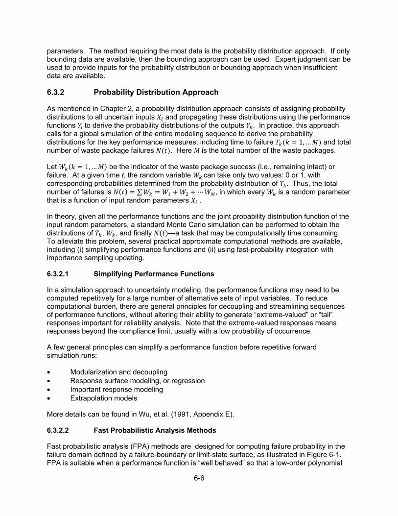
6-6

parameters. The method requiring the most data is the probability distribution approach. If only bounding data are available, then the bounding approach can be used. Expert judgment can be used to provide inputs for the probability distribution or bounding approach when insufficient data are available.

6.3.2 Probability Distribution Approach

As mentioned in Chapter 2, a probability distribution approach consists of assigning probability distributions to all uncertain inputs and propagating these distributions using the performance functions to derive the probability distributions of the outputs . In practice, this approach calls for a global simulation of the entire modeling sequence to derive the probability distributions for the key performance measures, including time to failure 1, … and total number of waste package failures . Here is the total number of the waste packages.

Let 1, … be the indicator of the waste package success (i.e., remaining intact) or failure. At a given time t, the random variable can take only two values: 0 or 1, with corresponding probabilities determined from the probability distribution of . Thus, the total number of failures is ∑ , in which every is a random parameter that is a function of input random parameters .

In theory, given all the performance functions and the joint probability distribution function of the input random parameters, a standard Monte Carlo simulation can be performed to obtain the distributions of , , and finally —a task that may be computationally time consuming. To alleviate this problem, several practical approximate computational methods are available, including (i) simplifying performance functions and (ii) using fast-probability integration with importance sampling updating.

6.3.2.1 Simplifying Performance Functions

In a simulation approach to uncertainty modeling, the performance functions may need to be computed repetitively for a large number of alternative sets of input variables. To reduce computational burden, there are general principles for decoupling and streamlining sequences of performance functions, without altering their ability to generate “extreme-valued” or “tail” responses important for reliability analysis. Note that the extreme-valued responses means responses beyond the compliance limit, usually with a low probability of occurrence.

A few general principles can simplify a performance function before repetitive forward simulation runs:

• Modularization and decoupling • Response surface modeling, or regression • Important response modeling • Extrapolation models

More details can be found in Wu, et al. (1991, Appendix E).

6.3.2.2 Fast Probabilistic Analysis Methods

Fast probabilistic analysis (FPA) methods are designed for computing failure probability in the failure domain defined by a failure-boundary or limit-state surface, as illustrated in Figure 6-1. FPA is suitable when a performance function is “well behaved” so that a low-order polynomial

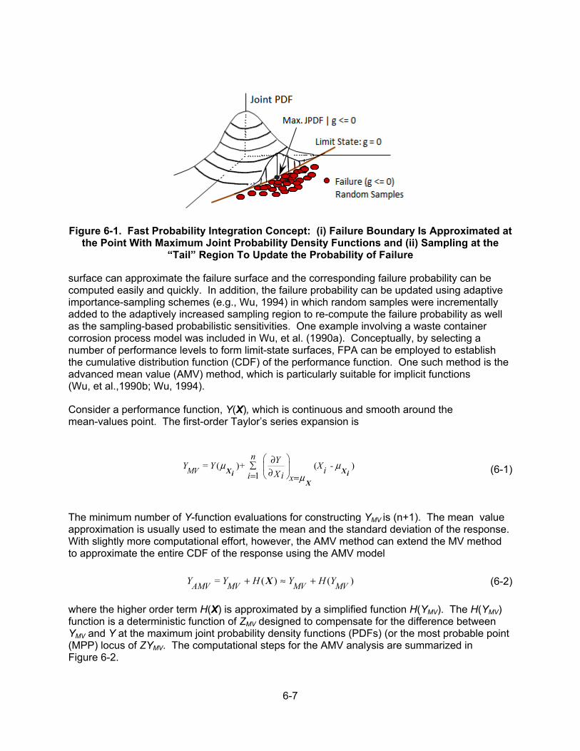
6-7

Figure 6-1. Fast Probability Integration Concept: (i) Failure Boundary Is Approximated at the Point With Maximum Joint Probability Density Functions and (ii) Sampling at the

“Tail” Region To Update the Probability of Failure

surface can approximate the failure surface and the corresponding failure probability can be computed easily and quickly. In addition, the failure probability can be updated using adaptive importance-sampling schemes (e.g., Wu, 1994) in which random samples were incrementally added to the adaptively increased sampling region to re-compute the failure probability as well as the sampling-based probabilistic sensitivities. One example involving a waste container corrosion process model was included in Wu, et al. (1990a). Conceptually, by selecting a number of performance levels to form limit-state surfaces, FPA can be employed to establish the cumulative distribution function (CDF) of the performance function. One such method is the advanced mean value (AMV) method, which is particularly suitable for implicit functions (Wu, et al.,1990b; Wu, 1994).

Consider a performance function, Y(X), which is continuous and smooth around the mean-values point. The first-order Taylor’s series expansion is

( )+ ( - )1MV

n YY = Y XiX ii xμ μ

μ

∂ ∂ = =X Xi i

X

(6-1)

The minimum number of Y-function evaluations for constructing YMV is (n+1). The mean value approximation is usually used to estimate the mean and the standard deviation of the response. With slightly more computational effort, however, the AMV method can extend the MV method to approximate the entire CDF of the response using the AMV model

( ) ( )AMV MV MV MVY = Y H Y H Y+ ≈ +X (6-2)

where the higher order term H(X) is approximated by a simplified function H(YMV). The H(YMV) function is a deterministic function of ZMV designed to compensate for the difference between YMV and Y at the maximum joint probability density functions (PDFs) (or the most probable point (MPP) locus of ZYMV. The computational steps for the AMV analysis are summarized in Figure 6-2.

6-8

Figure 6-2. Advanced Mean Value Method for Fast Cumulative Distribution Function Analysis

These FPA methods have been applied to several HLW-related example problems, as discussed in Section 6.4. 6.3.3 Bounding Approach

To implement the probability distribution approach, it is necessary to specify the joint distribution of all input parameters. If this can be done, then, in principle, the joint distribution of the responses can be calculated. Although there may be sufficient theoretical foundations or experimental data to specify the distribution of many input variables, it is likely that, for some input variables, no such information exists. Although some information about the distribution of such a parameter may exist based on theory, data, or expert judgment, this information may be too vague to justify assigning a distribution to X. However, in such a case, it may be possible to characterize X as lying in some specified uncertainty interval with high assurance. It is expected that the uncertainty interval and the level of assurance will be specified by expert judgment.

Assume that the set of input variables can be divided into two subsets - X' and X", where X' = {X1,...Xm} is a set of input variables with joint distribution F{x1,...xm} = Prob{X1 ≤ x1,...Xm ≤ xm}, and X" = {Xm+1,... , XL} is a set of input variables with uncertainty intervals [am+1,bm+1],...[aL,bL]. The bounding approach combines the input distribution F for X' with the uncertainty intervals for X" to calculate upper and lower bounds for the joint distribution of the output variables Y = Y1,...Ym}, without diminishing or enhancing the input uncertainties. A probabilistic inequality is used to relate the assurance level of the output bounds to the assurance levels of the input uncertainty intervals.

6-9

A note of caution is warranted.1 When an input variable X is characterized by an uncertainty interval , , it is assumed that not enough is known about X to justify specifying a distribution for it. Consequently, it would not be appropriate to replace the uncertainty interval with some fitted distribution. For example, some analysts might be tempted to replace an uncertainty interval , by a distribution for X (e.g., a lognormal, where is set equal to the assurance associated with the uncertainty interval). This would be inappropriate for several reasons. First, it would be substituting the analyst’s judgment for the experts’ judgment. Second, the use of any distribution implies an averaging process, which could lead to less uncertainty in the output distribution of Y than is implied by the uncertainty interval for X. Third, the tail behavior of the fitted distribution might possibly dominate the effect of X on the output distribution of Y, and this would violate the implicit judgment of the experts that nothing can be said about the values of X outside of the uncertainty interval.

6.3.4 Expert Judgment

The use of expert judgment (or expert opinion) can be an essential aspect of uncertainty modeling. Three areas of particular concern are scenario development, model development, and parameter estimation. In the area of scenario development, expert judgment can be important for identifying, classifying, and screening events and processes; formulating and screening scenarios; and estimating their relative ranking and probabilities of occurrence. In model development, expert judgment can be important for selecting and interpreting data, developing the conceptual models, and building confidence in the models and codes. In parameter estimation, expert judgment is also needed for identifying important parameters and quantifying their uncertainty. Specific techniques for the formal elicitation and use of expert judgment in these areas are discussed in Bonano, et al. (1990), and more recently in NRC (1995).

6.3.5 Sensitivity Analysis

Further to the discussions in Chapters 3 and 4, in engineering performance analysis, many sensitivity measures can be defined. A commonly used sensitivity measure in deterministic

analysis is performance sensitivity, , where is a performance function (e.g., time to failure)

and is a design variable. For probabilistic PA, a more relevant sensitivity measure is probability sensitivity, which measures the change in probability relative to the change in distribution parameters, such as mean and standard deviation. As discussed in Chapter 4, probabilistic sensitivity measures can be used to identify and rank important uncertainty parameters. The samples created by the importance sampling method mentioned in Section 6.3.2 can be used to compute probabilistic sensitivities using the CDF sensitivity method discussed in Chapter 4.

The concept of sensitivity analysis can be extended further to include all the assumptions that are uncertain. The uncertainty assumptions can include probability distribution types (e.g., lognormal and Weibull), process models (matrix flow, fracture flow), and parameters in an empirical life predictive model. The generalized sensitivity analysis can be used to identify those parameters and processes that must be examined with particular care, to ascertain that their contributions to performance uncertainty have been properly assessed.

1This caution agrees with the guidance from the Maximum Entropy Formalism (Section 2.2.3.3 of this report). The least biased estimate for the PDF with only the uncertainty interval now would be a uniform distribution between the two end points, as shown in Table 2-1.

6-10

6.4 Fast Probabilistic Performance Assessment Example

The FPA methods summarized in Section 6.3.2 were applied to EBS applications as reported in Wu and Nair (1988), which outlined an FPA computational framework for EBS performance analysis illustrated in Figure 6-3.

The FPA methodology was demonstrated using an EBS code called CONVO (Wu, et al., 1988) and waste container corrosion examples (Wu and Nair, 1989; Wu, et al., 1990b). As an example, Figure 6-4 compares the container life CDF computed using both the AMV and the Monte Carlo methods. There were 10 random parameters in the CONVO input. The CDF result using 10,000 random samples was similar to the AMV result using 19 CONVO runs.

Figure 6-3. A Fast Probabilistic Performance Assessment Computational Framework for Engineered Barrier System

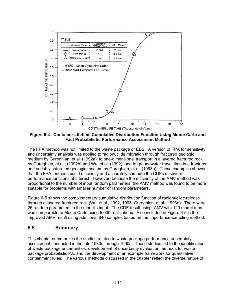
6-11

Figure 6-4. Container Lifetime Cumulative Distribution Function Using Monte Carlo and Fast Probabilistic Performance Assessment Method

The FPA method was not limited to the waste package or EBS. A version of FPA for sensitivity and uncertainty analysis was applied to radionuclide migration through fractured geologic medium by Gureghian, et al. (1992a); to one-dimensional transport in a layered fractured rock by Gureghian, et al., (1992b) and Wu, et al. (1992); and to groundwater travel time in a fractured and variably saturated geologic medium by Gureghian, et al. (1993b). These examples showed that the FPA methods could efficiently and accurately compute the CDFs of several performance functions of interest. However, because the efficiency of the AMV method was proportional to the number of input random parameters, the AMV method was found to be more suitable for problems with smaller number of random parameters. Figure 6-5 shows the complementary cumulative distribution function of radionuclide release through a layered fractured rock (Wu, et al., 1992, 1993; Gureghian, et al., 1993a). There were 25 random parameters in the model’s input. The CDF result using AMV with 129 model runs was comparable to Monte Carlo using 5,000 realizations. Also included in Figure 6-5 is the improved AMV result using additional 646 samples based on the importance-sampling method. 6.5 Summary This chapter summarizes the studies related to waste package performance uncertainty assessment conducted in the late 1980s through 1990s. These studies led to the identification of waste package uncertainties, development of uncertainty evaluation methods for waste package probabilistic PA, and the development of an example framework for quantitative containment rules. The various methods discussed in the chapter reflect the diverse nature of

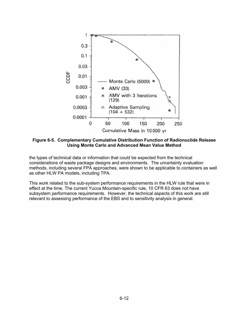
6-12

Figure 6-5. Complementary Cumulative Distribution Function of Radionuclide Release Using Monte Carlo and Advanced Mean Value Method

the types of technical data or information that could be expected from the technical considerations of waste package designs and environments. The uncertainty evaluation methods, including several FPA approaches, were shown to be applicable to containers as well as other HLW PA models, including TPA.

This work related to the sub-system performance requirements in the HLW rule that were in effect at the time. The current Yucca Mountain-specific rule, 10 CFR 63 does not have subsystem performance requirements. However, the technical aspects of this work are still relevant to assessing performance of the EBS and to sensitivity analysis in general.

7-1

7 SUMMARY AND CONCLUSIONS

The U.S. Nuclear Regulatory Commission (NRC), with assistance from the Center for Nuclear Waste Regulatory Analyses (CNWRA®), has conducted technical assessment, as documented in a technical evaluation report (TER), of the U.S. Department of Energy (DOE) analyses in a safety analysis report (SAR) to develop technical insights on the application of performance assessment in the context of geologic disposal. Preceding this assessment, NRC had numerous prelicensing interactions with DOE over a 20-year period to ensure a complete, high-quality license application from DOE for a defensible final decision of facility compliance (Eisenberg, et al., 1999). Total-system-level performance assessment (PA) has been the framework for understanding the repository system and for formulating questions for interactions with DOE. PA is the manifestation, in the field of nuclear waste management, of the Commission’s Probabilistic Risk Assessment policy statement and risk-graded approach, as envisioned in the mid-1990s, whereby the staff would use risk information to focus a licensee’s activities on those problems that pose the greatest risk to the public health and safety (NRC, 1997). The regulations in 10 CFR Part 63 (Code of Federal Regulations, 2001) for the High-Level Waste (HLW) program also have risk-based requirements, with particular emphasis on probabilistic PA that would give system-level understanding of the performance, particularly in terms of providing an understanding of the likely outcomes given uncertainties, sensitivities, interactions among the components and processes, and the capability of individual system components and processes (NRC, 2003; Callan, 1998). NRC’s HLW program took the initiative to (i) gather information on risk insights for effective prelicensing interactions with DOE and efficient review of the license application and (ii) train staff so they would specifically look for, among other things, identification and quantification of sources of uncertainty in the analysis and would relate the sensitivity of the results to key assumptions and uncertainties. This report summarizes various uncertainty and sensitivity analysis methods (previously existing as well as others NRC and CNWRA staffs developed) used for more than 20 years and documents the experience gained through the use and development of these methods. This report builds on the various uncertainty and sensitivity analyses methods discussed at a knowledge capture seminar held in Rockville, Maryland, in September 2007. NRC has carried out uncertainty and sensitivity analysis activities as long as PAs have been performed by NRC’s HLW program (since the early 1970s). Sandia National Laboratories developed a PA methodology for NRC to evaluate HLW disposal in a hypothetical repository, initially in bedded salt formations and later in other geologic media, namely basalt and tuff (Bonano, et al., 1989a; Gallegos, 1991; Eisenberg, 1999). Starting in the late 1980s, NRC staff developed independent PA capabilities through a series of Iterative Performance Assessment (IPA) phases: Phase I (Codell, et al., 1992), Phase II (Wescott, et al., 1995), and Phase III (planning) in 1995. Uncertainty and sensitivity became a part of NRC’s independent analyses starting with IPA Phase II and continued through the development and use of various versions of the TPA code (Versions 3.1, 3.1.3, 3.1.4, 3.2, 4.1, 5.0, and 5.1) to estimate the relative importance of key technical issues and integrated subissues. These efforts paralleled DOE’s PAs such as Total System Performance Assessment (TSPA)–Viability Assessment (DOE, 1998) and Total System Performance Assessment–Site Recommendation (CRWMS M&O, 2000). NRC’s uncertainty and sensitivity analyses were formally documented in several reports and NUREGs including NRC (1999) and Mohanty et al. (1999a, 2002). Each phase of uncertainty and sensitivity analyses enabled NRC staff to gradually move from preliminary models to more sophisticated and mature models, techniques, and corresponding insights. The following pages summarize the various uncertainty and sensitivity analysis methods NRC and CNWRA staffs have developed and used for the past 20 years.

7-2

7.1 Uncertainty Analysis The results from PA models are uncertain because of simplifying assumptions, randomness in processes, and uncertainty about the parameters. The main focus of uncertainty analysis is the characterization, representation and propagation of uncertainty through a model, and analysis its effects on the results. These areas are generally discussed in this report, but specific areas covered include representation and propagation of uncertainty in models, generation of a risk basis, random sampling, peak-of-the-mean criterion for risk, risk dilution, convergence of the risk curve, and granularity. The most typical representation of uncertainty is through model input parameters. Represented uncertainties are categorized as aleatory and epistemic. Aleatory is the uncertainty in the value of a parameter that comes about because of real randomness in the processes that cannot reasonably be specified in advance. Epistemic uncertainty is the uncertainty in the value of a parameter of a model that is fixed but unknown. Each Monte Carlo realization of the PA model was used to calculate the effects of both aleatory and epistemic uncertainty in the parameters that determine the model outcome. The parameter probability density functions (PDFs) need to be defensible especially because (i) uncertainty ranges that are too broad may cause risk dilution and (ii) uncertainty ranges that are too narrow may be unwarranted and cause bias in the results. A questionnaire was developed for all PA experts and process-level modelers to understand the PA model parameter needs. The questionnaire was used to obtain information required for a PDF at an appropriate level of technical basis and support with reasoned arguments. It promoted organized interactions between the process and system modelers and challenged process modelers to think more broadly and comprehensively. Methods such as the maximum entropy formalism can be used to estimate a distribution from the available information. However, the maximum entropy formalism will give the least biased PDF for the available data. In many cases, this implies the broadest PDF that is justified by the available information, and is not always the optimum choice for the PA because of the danger of “risk dilution.” Monte Carlo analysis is used to sample possible values of parameters from probability distributions. A modified sampling procedure, known as Latin Hypercube Sampling (LHS), is more advantageous because it forces a more even coverage of the sampled space. Convergence of model results to a smooth mean dose curve is important because it is the mean value of the dose that would be compared to the regulations. Depending on the models, a large number of realizations may be needed to reach a smooth, converged result. For the nominal scenario, where processes such as corrosion and groundwater transport are slow and predictable, convergence to a smooth mean dose curve is straightforward and requires only several hundred realizations. However, calculating the mean dose curve for disruptive event scenarios (e.g., volcanism, seismicity) can be challenging because the events are highly unlikely and can produce relatively large but short-lived doses. Special convolution-based calculations (see Section 2.2.7) were needed in some cases to compute a smooth function of time. Representation of spatial variability in the physical processes is often at a coarse level because of computational and time constraints. For example, the fraction of waste contacting infiltrating water can vary from location to location in the repository, but for computational expediency, this phenomenon must be captured by only a few representative waste packages. When the differences from package to package are not be captured adequately, the spatial discretization

7-3

level is considered too coarse or “grainy.” In some cases, the proper choice of input parameters can partially alleviate the granularity issue. 7.2 Sensitivity Analyses In the context of this report, sensitivity analysis (or uncertainty importance analysis) determines the influence of the various parts of the PA on the model results. These parts include the choice of the model, submodels, parameters, and system components. Parameter sensitivity analysis methods were used to identify model parameters for which a small input change can have a relatively large effect on estimated repository performance. This analysis allows the modeler to focus efforts to improve the PA by refining the model or its input parameters without devoting undue effort to unimportant areas. Parameter sensitivity analysis techniques used in the PA analyses are categorized as statistical and nonstatistical. Statistically based methods rely on some form of random sampling of input parameters to generate a set of responses from the PA models. They use statistical hypothesis testing to analyze the relationships between the input parameters and the model responses to make inferences about the most sensitive input parameters. Statistically based methods require a large set of model runs, but those are usually available from uncertainty analyses with the PA code. Analyses were performed on either the original input set or output value pairs, or this information was first altered by transformations to enhance the sensitivity calculations. Transformations used included normalization, rank transformation, logarithmic transformation, scaled-power transformation, standardization, and Gaussian transformation. Although transformations generally increase the goodness of fit analyses, they can also distort the meaning of the results if applied to the dependent variable (dose). Because risk is usually based on mean doses, regression results based on transformed variables should be used only on the independent variables. Regression methods are based on the correlation between the model result (e.g., peak dose) and the independent parameters under the assumption that they are related linearly. Stepwise multiple linear regression determines the most influential input parameters according to how much each input parameter reduces the residual sum of squares. Regression methods are most useful for monotonic relationships between model input and output. However, if the relationship is not monotonic, regression-based methods are at a severe disadvantage. A non-monotonic relationship can be highly correlated, but have a low correlation coefficient. Several tests that were found to be useful in determining the sensitivity of parameters not having monotonic dependence included (i) testing the location of output values dependent on input values, (ii) testing dispersion of output values dependent on input values, and (iii) testing the distribution of the output variable on the distribution of the input variable. These methods most suited to non-monotonic relations are covered in sections 3.2.2.3 and 4.7 of this report. Nonparametric sensitivity analyses included the Kolmogorov-Smirnov (K-S) test, the Sign test, and the Wilcoxon Rank Sum test. Nonparametric tests are statistical, but differ from regression tests because they do not require the assumption that the data have prespecified distributions (e.g., normal). Nonparametric methods were also used in the Regional Sensitivity Analysis (RSA) and the Strategic Partitioning of Assumption Ranges and Consequences (SPARC) method described next. Several advanced sensitivity analysis methods that were developed and/or used included Cumulative Distribution Function (CDF) Sensitivity Analysis, Genetic Algorithms, Regionalized Sensitivity Analysis, SPARC, Parameter Tree (PT) and Distribution Partitioning Intercept (DPI),

7-4

Morris, Fourier Amplitude Sensitivity Technique (FAST), and digital signal processing methods. Some of these are nonstatistical sensitivity analysis methods that exercised the PA models as a part of the methodology. The CDF sensitivity method (Mohanty and Wu, 2000, 2001; Wu and Mohanty, 2006) developed at the Southwest Research Institute® uses random samples at any designated quantile of the output CDF (i.e., not just the mean or median). The method also uses hypothesis testing for acceptance limits, introduced for the first time in the sensitivity analysis literature, and two different sensitivity measures to identify and rank influential random parameters. This approach provides a reliable alternative that can handle ill-behaved or highly nonlinear functions with nonnormally distributed parameters. Because the sample size needed does not depend on the number of sampled parameters, it is particularly suitable for complex models such as the TPA codes, with a large number of sampled parameters, only a few of which are significant. The genetic algorithm technique appears to have good power to identify important parameters, especially when the data are noisy. However, the analyst’s understanding of the initial results of the parameter screening is needed for a good final analysis to screen out the obviously spurious sensitivities. The RSA method (Osidele and Mohanty, 2006) uses binary classification of Monte Carlo model results and a K-S test to identify influential parameters. Binary classification segregates model results that conform to a prescribed output behavior (e.g., dose values above or below a regulatory limit). The PT method (Jarzemba and Sagar, 2000) was developed at CNWRA as a technique for identifying parameters that caused a performance metric (e.g., peak dose for a realization) to attain high values. A sensitivity index (Pensado, 2008) was developed to identify correlations between model input parameters and outputs. The DPI method was designed as an extension to the PT method, to define a sensitivity index as a statistic that would follow a continuous distribution, as opposed to the discrete distribution of the PT method. The DPI method avoids having to specify an arbitrary branching criterion needed by the PT method. In contrast with regression methods, both the PT and DPI methods yield results that are independent of changes of scale or transformations to inputs and outputs. Two other sensitivity methods NRC and CNWRA used were the Morris and FAST techniques, which are not detailed here because they are adequately documented in the open literature. Rankings for parameter sensitivity employed multiple techniques. Because rankings differed among techniques, an ad hoc method was developed to collate the results in order to select the top 10 to 20 parameters, especially during the early iterations of PAs when the impact of various parameters and their associated conservatism were not well known. It was equally important to verify that the sensitive parameters were correctly identified. This was done by calculating and comparing Monte Carlo results from the originally designated list of sampled parameters against new Monte Carlo results for which only the reduced set of sensitive parameters were either included (i.e., sampled) or eliminated (i.e., fixed at a constant value). Keeping only the most sensitive parameters as sampled parameters gave results similar to the basecase results. Removing the most sensitive parameters from sampling reduced most of the uncertainty in the results.

7-5

Aside from parameter sensitivity, a variety of methods were used to understand system sensitivity. These included distributional sensitivity, digital signal processing, SPARC, and component sensitivity analysis methods. Distributional sensitivity analysis was not used directly to rank sensitive variables but to determine the effect of estimation of parameter distributions on the performance results. In this technique, the input distributions were changed either by shifting the mean of a distribution by a predetermined percentage or changing the shape of the distribution while keeping the minimum and maximum fixed. The distributional analyses can reveal improper choices of distribution functions that can affect the dose response significantly. The digital signal processing technique NRC staff developed analyzed PA results to determine barrier effectiveness. Using averaged radionuclide release rates from the engineered barrier system, the unsaturated zone, and the saturated zone, the method identified the particular barriers important to overall performance. The method did not appear to work well on individual Monte Carlo realizations, because of the noisiness of the signals. The SPARC method is based on ideas of reactor probabilistic risk assessment (PRA) that aim to extract information on what sets of model parameter values taken together could produce substantially increased doses (SIDs). The method also determines whether repository features working alone or in combination with other features could protect the repository from SIDs even under extreme conditions that are highly unlikely. The component sensitivity analysis method looks at the whole component of a system at once, either performing or not performing. Component sensitivity analysis allows the exploration of the resiliency of components that would not be evident unless the other components have failed. Component failure is simulated by changing input parameters to degrade the performance severely (e.g., setting the alluvium distance to zero), either one at a time or in combination with other components. The method can show some interesting interactions as well as redundancy in the system when selected components are forced to fail. 7.3 Model Conservatism Study PA models often have conservative assumptions about the values of the parameters due to the tendency to err on the side of safety when data on a process or phenomenon are inadequate. Analyses were conducted to illustrate how conservatism can influence the sensitivity based ranking of influential parameters. The study illustrated that depending on the performance model, sensitivity could change nonlinearly with the level of conservatism dictated by the choice of parameter values. As a result, the sensitivity based ranking of influential parameters can change non-monotonically with the assumed level of conservatism. Dependence of the ranking of influential parameters on conservative assumptions could lead an analyst to conclude that other parameters are more influential. Therefore, analysts should evaluate the effects of the assumed degree of conservatism to ensure that influential parameters are correctly identified. 7.4 Earlier Activities Related to Waste Package A number of uncertainty and sensitivity analysis methods were used during the early stage of the repository program (late 1980s). The focus was on waste package performance, and the applicable regulation at the time was 10 CFR Part 60, which had a “substantially complete containment” (SCC) requirement. Four uncertainty evaluation methods—probability distribution

7-6

approach, bounding approach, expert judgment, and sensitivity analysis—were identified as elements of a probability based framework that, without either diminishing or enhancing the input uncertainties, can provide quantitative measures for assessing waste package design performance. The study reflected on the diverse types of technical information that could be expected for conducting waste package PA. It identified uncertainties and characterized them by uncertainty types and sources as a precursor to quantification. The methodologies covered at the time were of general nature and not exhaustive. It was recognized that long-term containment analysis for the waste packages would require a probabilistic framework based on a good understanding of the physical, chemical, geological, and other aspects. 7.5 Conclusions Overall, uncertainty and sensitivity analyses, conducted primarily as a part of PA, helped NRC staff prioritize reviews and determine key areas for interactions with DOE. At a programmatic level, the analysis capability enabled NRC staff to interact more effectively with DOE on its Total System Performance Assessments developed during the prelicensing activities; to formulate a risk-informed, site-specific standard; and to develop appropriate guidance documents. It helped NRC and CNWRA staffs to develop experience and insights necessary for effective prelicensing interactions and review of DOE’s Safety Analysis Report. At a technical level, these analyses have helped NRC staff to develop insights about important features, events, and processes (FEPs) that needed further careful assessment and decide which portions of the DOE assessment required focus through further detailed quantitative analyses to successfully demonstrate compliance with the safety standard. Some of the areas prompted by uncertainty and sensitivity analyses for discussion included modeling assumptions, conceptual models, data needs, revisions to the site characterization program, and decisions on the use of expert judgment versus additional data collection. The present document is an attempt to capture knowledge from over 20 years of effort by the NRC and CNWRA staffs on sensitivity and uncertainty analyses, primarily with regard to the proposed disposal of high-level radioactive waste at Yucca Mountain. In most cases, the individual sensitivity analysis methods presented in this document come without strong recommendations concerning their usefulness or accuracy. In fact, Chapter 5 expounds on the desirability of judging the sensitivity of parameters based on a consensus formed from the results of multiple techniques. The main reason for this approach was to identify as many influential parameters as practical within a certain specified sensitivity criterion and then eliminate those parameter results that turn out to be spurious. This approach was intended to avoid missing an influential parameter in the analysis, rather than to avoid misidentifying a non-influential parameter as influential. At the early iterations of performance assessments, this approach was useful because further understanding of the modeled system behavior was needed. However, with further interations of performance assessment, as the analysts developed better understanding of the system, some of the methods were no longer as useful because simpler methods provided equally good results. For example, after many iterations of performance assessments, it became clearer that certain methods presented in Chapters 3 (section 3.2.2.3) and 4 (section 4.7) were more advantageous than other methods for non-monotonic relationships between the independent and dependent variables. The methods presented in this report and the experience gained over more than two decades of work by NRC and CNWRA staffs are general enough to find broad applications across other NRC activities such as low-level waste disposal.

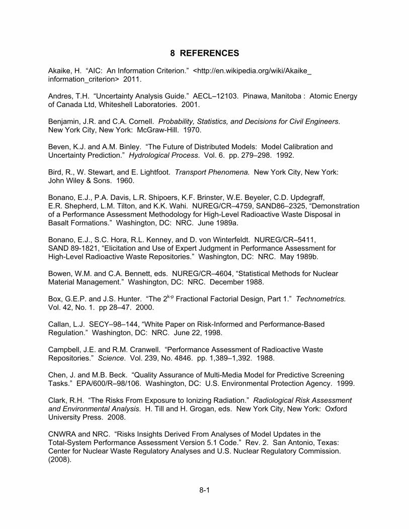
8-1

8 REFERENCES

Akaike, H. “AIC: An Information Criterion.” <http://en.wikipedia.org/wiki/Akaike_ information_criterion> 2011. Andres, T.H. “Uncertainty Analysis Guide.” AECL–12103. Pinawa, Manitoba : Atomic Energy of Canada Ltd, Whiteshell Laboratories. 2001. Benjamin, J.R. and C.A. Cornell. Probability, Statistics, and Decisions for Civil Engineers. New York City, New York: McGraw-Hill. 1970. Beven, K.J. and A.M. Binley. “The Future of Distributed Models: Model Calibration and Uncertainty Prediction.” Hydrological Process. Vol. 6. pp. 279–298. 1992. Bird, R., W. Stewart, and E. Lightfoot. Transport Phenomena. New York City, New York: John Wiley & Sons. 1960. Bonano, E.J., P.A. Davis, L.R. Shipoers, K.F. Brinster, W.E. Beyeler, C.D. Updegraff, E.R. Shepherd, L.M. Tilton, and K.K. Wahi. NUREG/CR–4759, SAND86–2325, “Demonstration of a Performance Assessment Methodology for High-Level Radioactive Waste Disposal in Basalt Formations.” Washington, DC: NRC. June 1989a. Bonano, E.J., S.C. Hora, R.L. Kenney, and D. von Winterfeldt. NUREG/CR–5411, SAND 89-1821, “Elicitation and Use of Expert Judgment in Performance Assessment for High-Level Radioactive Waste Repositories.” Washington, DC: NRC. May 1989b. Bowen, W.M. and C.A. Bennett, eds. NUREG/CR–4604, “Statistical Methods for Nuclear Material Management.” Washington, DC: NRC. December 1988. Box, G.E.P. and J.S. Hunter. “The 2k-p Fractional Factorial Design, Part 1.” Technometrics. Vol. 42, No. 1. pp 28–47. 2000. Callan, L.J. SECY–98–144, “White Paper on Risk-Informed and Performance-Based Regulation.” Washington, DC: NRC. June 22, 1998. Campbell, J.E. and R.M. Cranwell. “Performance Assessment of Radioactive Waste Repositories.” Science. Vol. 239, No. 4846. pp. 1,389–1,392. 1988. Chen, J. and M.B. Beck. “Quality Assurance of Multi-Media Model for Predictive Screening Tasks.” EPA/600/R–98/106. Washington, DC: U.S. Environmental Protection Agency. 1999. Clark, R.H. “The Risks From Exposure to Ionizing Radiation.” Radiological Risk Assessment and Environmental Analysis. H. Till and H. Grogan, eds. New York City, New York: Oxford University Press. 2008. CNWRA and NRC. “Risks Insights Derived From Analyses of Model Updates in the Total-System Performance Assessment Version 5.1 Code.” Rev. 2. San Antonio, Texas: Center for Nuclear Waste Regulatory Analyses and U.S. Nuclear Regulatory Commission. (2008).

8-2

Code of Federal Regulations. “Disposal of High-Level Radioactive Wastes in a Proposed Geological Repository at Yucca Mountain, Nevada.” Title 10—Energy, Chapter 1–NRC, Part 63. Washington, DC: U.S. Government Printing Office. 2002. Code of Federal Regulations. “Public Health and Environmental Radiation Protection Standards for Yucca Mountain, Nevada.” Title 40—Protection of Environment, Chapter 1–EPA, Part 197. Washington, DC: U.S. Government Printing Office. 2001. Code of Federal Regulations. “Disposal of High-Level Radioactive Wastes in Geological Repositories.” Title 10—Energy, Chapter 1—NRC, Part 60. Washington, DC: U.S. Government Printing Office. 1991. Codell, R.B, N. Eisenberg, D. Fehringer, W. Ford, T. Margulies, T. McCartin, J. Park, and J. Randall. NUREG–1327, “Initial Demonstration of the NRC’s Capability to Conduct a Performance Assessment for a High-Level Waste Repository.” Washington, DC: NRC. May 1992. Codell, R.B., M.R. Byrne, T.J. McCartin, S. Mohanty, J. Weldy, M. Jarzemba, G.W. Wittmeyer, Y. Lu, and R.W. Rice, NUREG–1746, “System-Level Repository Sensitivity Analyses, Using TPA Version 3.2 Code.” Washington, DC: U.S. Nuclear Regulatory Commission. 2001. Codell, R. and D. Esh. “The Interpretation of Risk and Sensitivity Under the Peak-of-the-Mean Concept.” PSAM-7 Conference, Berlin Germany, June 14–18, 2004. International Association for Probabilistic Safety Assessment and Management Conference Proceedings. London, England: Springer-Verlag London Ltd. 2004. Conesa, A., M.J. Nueda, A. Alberto, A. Ferrer, and T. Talon. “maSigPro: A Method to Identify Significant Differential Expression Profiles in Time-Course Microarray Experiments.” 2005. <HTTP://www.ivia.es/centrogenomica/bioinformatics.htm, maSigPro_1.6.zip> (31 May 2011). Conover, W.J. Practical Nonparametric Statistics. New York City, New York: John Wiley & Sons. 1999. Cook, R. and S. Weisberg. An Introduction to Regression Graphics. New York City, New York: John Wiley & Sons. 1994. Corbett, J.O. “Risk Assessment Criteria for Radioactive Waste Disposal.” Risk Analysis. Vol. 8, No. 4. 1988. Cragnolino, G., N. Sridhar, J. Walton, R. Janetzke, T. Torng, Y.-T. Wu, and P. Nair. “Substantially Complete Containment—Example Analysis of a Reference Container.” CNWRA 94 003. San Antonio, Texas: CNWRA. January 1994. CRAN, Comprehensive R Archive Network, http://cran.r-project.org. 2011 CRWMS M&O. “Total System Performance Assessment for Site Recommendation.” TDR–WIS–PA–000001. Rev 00, ICN 01. MOL.20001220.0045. Las Vegas, Nevada: CRWMS M&O. 2000.

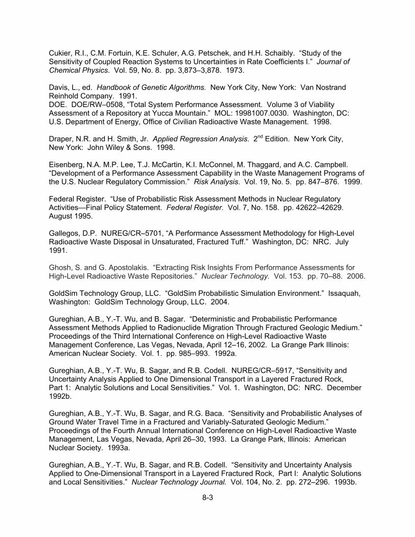
8-3

Cukier, R.I., C.M. Fortuin, K.E. Schuler, A.G. Petschek, and H.H. Schaibly. “Study of the Sensitivity of Coupled Reaction Systems to Uncertainties in Rate Coefficients I.” Journal of Chemical Physics. Vol. 59, No. 8. pp. 3,873–3,878. 1973. Davis, L., ed. Handbook of Genetic Algorithms. New York City, New York: Van Nostrand Reinhold Company. 1991. DOE. DOE/RW–0508, “Total System Performance Assessment. Volume 3 of Viability Assessment of a Repository at Yucca Mountain.” MOL: 19981007.0030. Washington, DC: U.S. Department of Energy, Office of Civilian Radioactive Waste Management. 1998. Draper, N.R. and H. Smith, Jr. Applied Regression Analysis. 2nd Edition. New York City, New York: John Wiley & Sons. 1998. Eisenberg, N.A. M.P. Lee, T.J. McCartin, K.I. McConnel, M. Thaggard, and A.C. Campbell. “Development of a Performance Assessment Capability in the Waste Management Programs of the U.S. Nuclear Regulatory Commission.” Risk Analysis. Vol. 19, No. 5. pp. 847–876. 1999. Federal Register. “Use of Probabilistic Risk Assessment Methods in Nuclear Regulatory Activities—Final Policy Statement. Federal Register. Vol. 7, No. 158. pp. 42622–42629. August 1995. Gallegos, D.P. NUREG/CR–5701, “A Performance Assessment Methodology for High-Level Radioactive Waste Disposal in Unsaturated, Fractured Tuff.” Washington, DC: NRC. July 1991. Ghosh, S. and G. Apostolakis. “Extracting Risk Insights From Performance Assessments for High-Level Radioactive Waste Repositories.” Nuclear Technology. Vol. 153. pp. 70–88. 2006. GoldSim Technology Group, LLC. “GoldSim Probabilistic Simulation Environment.” Issaquah, Washington: GoldSim Technology Group, LLC. 2004. Gureghian, A.B., Y.-T. Wu, and B. Sagar. “Deterministic and Probabilistic Performance Assessment Methods Applied to Radionuclide Migration Through Fractured Geologic Medium.” Proceedings of the Third International Conference on High-Level Radioactive Waste Management Conference, Las Vegas, Nevada, April 12–16, 2002. La Grange Park Illinois: American Nuclear Society. Vol. 1. pp. 985–993. 1992a. Gureghian, A.B., Y.-T. Wu, B. Sagar, and R.B. Codell. NUREG/CR–5917, “Sensitivity and Uncertainty Analysis Applied to One Dimensional Transport in a Layered Fractured Rock, Part 1: Analytic Solutions and Local Sensitivities.” Vol. 1. Washington, DC: NRC. December 1992b. Gureghian, A.B., Y.-T. Wu, B. Sagar, and R.G. Baca. “Sensitivity and Probabilistic Analyses of Ground Water Travel Time in a Fractured and Variably-Saturated Geologic Medium.” Proceedings of the Fourth Annual International Conference on High-Level Radioactive Waste Management, Las Vegas, Nevada, April 26–30, 1993. La Grange Park, Illinois: American Nuclear Society. 1993a. Gureghian, A.B., Y.-T. Wu, B. Sagar, and R.B. Codell. “Sensitivity and Uncertainty Analysis Applied to One-Dimensional Transport in a Layered Fractured Rock, Part I: Analytic Solutions and Local Sensitivities.” Nuclear Technology Journal. Vol. 104, No. 2. pp. 272–296. 1993b.

8-4

Harr, M. Reliability-Based Design in Civil Engineering. New York City, New York: McGraw-Hill. 1987. Helton, J.C. and F.J. Davis. “Sampling-Based Methods.” Sensitivity Analysis. A. Saltelli, K. Chan, and M. Scott, eds. Chichester, England: John Wiley & Sons Ltd. pp. 101–153. 2000. Helton, J.C., J.W. Garner, R.D. McCurley, and D.K. Rudeen. “Sensitivity Analysis Techniques and Results for Performance Assessment at the Waste Isolation Pilot Plant.” SAND90–7103. Albuquerque, New Mexico: Sandia National Laboratories. 1991. Hornberger, G.M. and R.C. Spear. “An Approach to the Preliminary Analysis of Environmental Systems.” Journal of Environmental Management. Vol. 12, No. 7. 1981. Hornberger, G.M., K.J. Beven, B.J. Cosby, and D.E. Sappington. “Shenandoah Watershed Study: Calibration of a Topography-Based, Variable Contributing Area Hydrological Model to a Small Forested Catchment.” Water Resources Research. Vol. 21, No. 12. pp. 1,841–1,850. 1985. Hornick, K. “The R FAQ—Frequently Asked Questions on R.” <http://CRAN.R-Project.org/doc/FAQ/> ISBN3-900051-08-9. 2007 Iman, J. “Stepwise Regression With PRESS and Rank Regression Program User’s Guide.” SAND79–1472. Albuquerque, New Mexico: Sandia National Laboratories. 1980. Iman, R. and J. Conover. “A Measure of Top-Down Correlation.” Technometrics. Vol. 29, No 3. pp. 351–357. August 1987. Iman, R.L. and M.J. Shortencarier. NUREG/CR–3624, SAND83–2365, “A FORTRAN 77 Program and User’s Guide for the Generation of Latin Hypercube and Random Samples for Use With Computer Models.” Washington, DC: NRC. March 1984. Iman, R., J. Davenport, E. Frost, and M. Shortencarier. “Stepwise Regression With PRESS and Rank Regression (Program User’s Guide).” SAND79–1472. Albuquerque, New Mexico: Sandia National Laboratories. 1980. Jarzemba, M.S. and B. Sagar. “A Parameter Tree Approach to Estimating System Sensitivities to Parameter Sets.” Reliability Engineering and System Safety. Vols. 67, 89. p. 102. 2000. Karamchandani, A. “New Methods in Systems Reliability.” Ph.D. dissertation. Stanford University. Palo Alto, California. 1990. Kaplan, S. and B.J. Garrick. “On the Quantitative Definition of Risk.” Risk Analysis. Vol. 1, No. 11. 1981. Kirchner, T.B. “Estimating and Applying Uncertainty in Assessment Models.” Radiological Risk Assessment and Environmental Analysis. J.E. Till and H.A. Grogan, eds. New York City, New York: Oxford University Press. 2008. Kleijnen, P.C. and J.C. Helton. “Statistical Analyses of Scatterplots To Identify Important Factors in Large-Scale Simulations.” SAND–98–2202. Albuquerque, New Mexico: Sandia National Laboratories. April 1999.

8-5

Lence, B.J. and A.K. Takyi. “Data Requirements for Seasonal Discharge Programs: An Application of a Regionalized Sensitivity Analysis.” Water Resources Research. Vol. 28, No. 7. pp. 781–1,789. 1992. Leslie, B.W., C. Grossman, and J. Durham, coords. “Total-System Performance Assessment (TPA) Version 5.1 Code Module Descriptions and User Guide.” ML080510329. San Antonio, Texas: CNWRA. 2007. Lu, Y. and S. Mohanty. “Sensitivity Analysis of a Complex, Proposed Geologic Waste Disposal System Using the Fourier Amplitude Sensitivity Test Method.” Reliability Engineering and System Safety. Vol. 72, No. 3. pp. 275–291. 2001. Madsen, H.O., S. Krenk, and N.C. Lind. Methods of Structural Safety. Englewood Cliffs, New Jersey: Prentice Hall, Inc. 1986. Manaktala, H.K. and C.G. Interrante. “Technical Considerations for Evaluating Substantially Complete Containment of HLW Within the Waste Package.” CNWRA 90-001. San Antonio, Texas: CNWRA. 1990. Manaktala, H., Y.-T. Wu, and P.K. Nair. “Technical Considerations and Approach for Evaluating Substantially Complete Containment of High-Level Nuclear Waste.” Proceedings of the International Topical Meeting on High-Level Radioactive Waste Management, Las Vegas, Nevada. La Grange Park, Illinois: American Nuclear Society. 1990. Mason, R.L., R.F. Gunst, and J.L. Hess. Statistical Design & Analysis of Experiments With Applications to Engineering and Science. New York City, New York: John Wiley & Sons. 1989. MathSoft, Inc. “STATSCI—S-Plus Reference Manual.” Seattle, Washington: MathSoft, Inc., StatSci Division. 1993 McCartin, T., R. Codell, S. Mohanty, R.G. Baca, V. Colten Bradley, J. Firth, M.R. Byrne, R. Janetzke, and M. Jarzemba. “U.S. NRC’s Performance Assessment Capability.” Proceedings of the Eighth International Conference on High-Level Radioactive Waste Management, Las Vegas, Nevada, May 11–14, 1998. La Grange Park, Illinois: American Nuclear Society. p. 13. 1998. Mohanty, S. and R. Codell. “Ramifications of Risk Measures in Implementing Quantitative Performance Assessment for the Proposed Radioactive Waste Repository at Yucca Mountain, Nevada, USA.” Risk Analysis. Vol. 24, No. 3. 2004. Mohanty, S. and R. Codell. “A Performance Assessment Review Tool for the Proposed Radioactive Waste Repository at Yucca Mountain, Nevada, USA.” Proceedings of the Probabilistic Safety Assessment and Management Conference (PSAM 5), Osaka, Japan, November 27–December 1, 2000. S. Kondo and K. Furuta, eds. Frontiers Science Series No. 34. Tokyo, Japan: Universal Academy Press, Inc. Vol. 3. pp. 1,485–1,593. 2000. Mohanty, S. and T.J. McCartin, coords. NUREG–1668, “NRC Sensitivity and Uncertainty Analyses for a Proposed HLW Repository at Yucca Mountain, Nevada, Using TPA 3.1. Volume I: Conceptual Models and Data.” Washington, DC: U.S. Nuclear Regulatory Commission. 2000.

8-6

Mohanty, S. and T.J. McCartin. “Total-system Performance Assessment (TPA) Version 3.2 Code: Module Description and User’s Guide.” San Antonio, Texas: CNWRA. 1998. Mohanty, S. and R. Nes. “The Effect of Model Conservatism on Identifying Influential Parameters.” Presentation at the PSAM 8 Conference, New Orleans, Louisiana, May 14–19, 2006. International Association for Probabilistic Safety and Management. 2006. Mohanty, S. and Y.-T. Wu. “CDF Sensitivity Analysis Technique for Ranking Influential Parameters in the Performance Assessment of the Proposed High-Level Waste Repository at Yucca Mountain, Nevada, USA.” Reliability Engineering and System Safety. Vol. 73/2. pp. 167–176. 2001. Mohanty, S. and Y.-T. Wu. “Sensitivity Analysis Technique for Ranking Influential Parameters in the Performance Assessment of the Proposed High-Level Waste Repository at Yucca Mountain, Nevada, USA.” Proceedings of ESREL 2000 Conference, Edinburgh, United Kingdom, May 14–17, 2000. D.W. Cottam, R.P. Pape, and J. Tait, eds. London, England: A.A. Balkema Publishers. 2000. Mohanty, S., R. Codell, J. Menchaca, R. Janetzke, M. Smith, P. LaPlante, M. Rahimi, and A. Lozano. “System Level Performance Assessment of the Proposed Repository at Yucca Mountain Using the TPA Version 4.1 Code.” CNWRA 2002-05. San Antonio, Texas: Center for Nuclear Waste Regulatory Analyses. March 2004a. Mohanty, S., B. Sagar, R. Janetzke, G. Wittmeyer, and W. Patrick. “Role of Component Sensitivity Analysis in the Risk Assessment of a Large and Complex System.” Presented at the PSAM 7/ESREL’04 Conference, Berlin, Germany, June 14–18, 2004. International Association for Probabilistic Safety and Management. 2004b. Mohanty, S., T.J. McCartin, and D.W. Esh. “Total-system Performance Assessment (TPA) Version 4.0 Code: Module Descriptions and User’s Guide.” San Antonio, Texas: CNWRA. 2002. Mohanty, S., R. Codell, R.W. Rice, J. Weldy, Y. Lu, R.M. Byrne, T.J. McCartin, M.S. Jarzemba, and G.W. Wittmeyer. “System-Level Repository Sensitivity Analyses Using TPA Version 3.2 Code.” CNWRA 99-002. San Antonio, Texas: CNWRA. 1999a. Mohanty, S., Y. Lu, and J.M. Menchaca. “Preliminary Analysis of the Morris Method for Identifying Influential Parameters.” American Nuclear Society Transactions. Vol. 81. p. 55. 1999b. Montgomery, D.C. Design and Analysis of Experiments. 5th Edition. New York City, New York: John Wiley & Sons. 2000. Morris, M.D. “Factorial Sampling Plans for Preliminary Computational Experiments.” Technometrics. Vol. 33, No. 2. pp. 161–174. 1991. Nair, P.K. and E. Tschoepe. “Substantially Complete Containment Feasibility Study Recommendations Report.” San Antonio, Texas: CNWRA. 1990. NeuralWare. “NeuralWorks Predict® Product Version 2.40.” Carnegie, Pennsylvania: NeuralWare. 2001.

8-7

Nicholson, T.J., J.E. Babendreir, P.S. Meyer, S. Mohanty, B.B. Hicks, and G.H. Leavesley, eds. NUREG/CP–0187, “Sensitivity Analysis Approaches, Applications, and Lessons. Washington, DC: NRC. 2004. NRC. NUREG–1762, “Integrated Issue Resolution Status Report.” Rev. 1. Washington, DC: U.S. Nuclear Regulatory Commission. 2004. NRC. NUREG–1804, “Yucca Mountain Review Plan.” Rev. 2. Washington, DC: U.S. Nuclear Regulatory Commission. 2003. NRC. NUREG–1668, “NRC Sensitivity and Uncertainty Analyses for a Proposed HLW Repository at Yucca Mountain, Nevada Using TPA 3.1. Volume II: Results and Conclusions.” Washington, DC: NRC. March 1999. NRC. COMSECY–96–061, “Staff Requirements––Risk-Informed, Performance-Based Regulation (DSI–12).” Washington, DC: U.S. Nuclear Regulatory Commission. 1997. NRC. NUREG–1563, “Branch Technical Position on the Use of Expert Elicitaiton in the High-Level Radioactive Waste PRogram.” Washington, DC: NRC. November 1996. Osidele, O.O. and M.B. Beck. “Food Web Modeling for Investigating Ecosystem Behaviour in Large Reservoirs of the South-Eastern United States: Lessons From Lake Lanier, Georgia.” Ecological Modelling. Vol. 173. pp. 129–158. 2004. Osidele, O.O. and S. Mohanty. “Application of Regionalized Sensitivity Analysis to a Performance Assessment Model of a High-Level Waste Repository.” Proceedings of the International High-Level Radioactive Waste Management Conference, Las Vegas, Nevada. La Grange Park, Illinois: American Nuclear Society. CD ROM. 2006. Osidele, O.O., W. Zeng, and M.B. Beck. “Coping With Uncertainty: A Case Study in Sediment Transport and Nutrient Load Analysis.” Journal of Water Resources Planning and Management. Vol. 129, No. 4. pp. 345–355. 2003. Pensado, O. “Use of Robust Sensitivity Indices To Analyze the Structure of Stochastic Performance Assessment Models.” Proceedings of the 12th International High-Level Radioactive Waste Management Conference, Las Vegas, Nevada, September 7–11, 2008. La Grange Park, Illinois: American Nuclear Society. CD ROM. pp. 582–587. 2008. Pensado, O. and B. Sagar. “Sensitivity Analysis of an Engineered Barrier System Model for the Potential Repository System in the United States.” Proceedings of the 7th International Conference on Probabilistic Safety Assessment and Management, Berlin, Germany, June 14–18, 2004. C. Spitzer, U. Schmocker, and V.N. Dang, eds. Vol. 6. London, United Kingdom: Springer-Verlag. pp. 3,123–3,129. 2004. Pensado, O., V. Troshanov, B. Sagar, and G. Wittmeyer. “A Partitioning Method for Identifying Model Parameters.” Proceedings of the Probabilistic Safety Assessment and Management (PSAM6) Conference. E.J. Bonano, A.L. Camp, M.J. Majors, and R.A. Thompson, eds. Kidlington, Oxford, United Kingdom: Elsevier Science Ltd. pp. 827–833. 2002. Press, W.H., S.A. Teukolsky, W. T. Vettering, and B.R. Flannery. Numerical Recipes. New York City, New York: Cambridge University Press. 1992

8-8

Provan, J.W. and E.S. Rodriguez, III. “Part I: Development of a Markov Description of Pitting Corrosion.” Corrosion Science. Vol. 45, No. 3. pp. 178–192. March 1989. Rice, R. “Risk Prediction and Design of Disposal Systems.” Ph.D. Thesis. University of Texas. El Paso, Texas. 2004 Rice, R. and S. Mohanty. “Total-system Performance Assessment Code for the Proposed High-Level Waste Repository at Yucca Mountain—Code Development and Lessons Learned.” Proceedings of the 2000 Waste Management Conference, Tucson, Arizona, October 2–4, 2000. Tucson, Arizona: Waste Management Symposia, Inc. CD Publication. 2000. Rodriguez, III, E.S. and J.W. Provan. “Part II: Development of a General Failure Control System for Estimating the Reliability of Deteriorating Structures.” Corrosion Science. Vol. 45, No. 3. pp. 193–206. March 1989. Sato, N. “Stochastic Process of Chloride Pit Generation in Passive Stainless Steel.” Electrochemical Science and Technology. Vol. 123, No. 8. 1976. Sato, E., H. Abo, and T. Murata. “Life Time Estimation and Accelerated Stress Corrosion Cracking Test of Stainless Steel in a Neutral Chloride Environment.” Corrosion 89 Conference, April 17–21, 1989. Paper No. 97. Houston, Texas: NACE. 1989. Shannon, C.E. “A Mathematical Theory of Communication.” Bell System Technical Journal. Vol. 27. pp. 379–423. October 1948. Shibata, T. and T. Takeyama. “Stochastic Theory of Pitting Corrosion.” Corrosion. Vol. 33, No. 7. pp. 243–251. 1977. Shortencarier, M. and J. Helton. “A FORTRAN 77 Program and User’s Guide for the Statistical Analyses of Scatterplots To Identify Important Factors in Large-Scale Simulations.” SAND99–1058. Albuquerque, New Mexico: Sandia National Laboratories. 1999. Smith, M., T.J. McCartin, and S. Mohanty. “TPA 3.2 Code’s Capability To Evaluate the Effects of Human Intrusion.” American Nuclear Society Transactions. Vol. 81. p. 53. 1999. Spear, R.C. and G.M. Hornberger. “Eutrophication in Peel Inlet—II: Identification of Critical Uncertainties via Generalized Sensitivity Analysis.” Water Research. Vol. 14. pp. 43–49. 1980. Spear, R.C., T.M. Grieb, and N. Shang. “Parameter Uncertainty and Interaction in Complex Environmental Models.” Water Resources Research. Vol. 30, No. 11. pp 3,159–3,169. 1994. Sridhar, N., G. Cragnolino, P.K. Nair, Y.-T. Wu, and C. Chang. “High-Level Waste Container Performance Models—Status and Current Developments.” Proceedings of the FOCUS '91 Conference, Las Vegas, Nevada, September 29–October 2, 1991. La Grange Park Illinois: American Nuclear Society. pp. 162–267. 1991. U.S. Environmental Protection Agency. “40 CFR Part 191 Environmental Radiation Protection Standards for the Management and Disposal of Spent Nuclear Fuel, High-Level and Transuranic Radioactive Wastes—Final Rule.” Federal Register. Vol. 58, No. 242. Washington, DC: Office of Radiation and Indoor Air. pp. 66398–66416. 1993.

8-9

Vose. “Maximum Entropy Formalism.” <http://www.vosesoftware.com/ModelRiskHelp/ Modeling_expert_opinion/> (2 April 2011). Weisstein, E.W. “Regularized Beta Function.” MathWorld—A Wolfram Web Resource. <http://mathworld.wolfram.com/RegularizedBetaFunction.html. 2011>. 2011. Weldy, J.R., M. Rahimi, and S. Mohanty. “Assessing the Consequences of an In-Package Criticality Event at a High-Level Nuclear Waste Repository.” Poster presented at the Annual Health Physics Society Meeting, Cleveland, Ohio, June 10–14, 2001. McLean, Virginia: Health Physics Society. 2001. Wescott, R.G., M.P. Lee, N.A. Eisenberg, T.J. McCartin, and R.G. Baca, eds. “NUREG–1464, “NRC Iterative Performance Assessment Phase 2.” Washington, DC: NRC. October 1995. Woo, H.H. and F.A. Simonen. “The Impact of In-Service Inspection on the Reliability of Nuclear Piping.” Advances in Probabilistic Fracture Mechanics. C. Sundararajan, ed. ASME PVP. Vol. 92. New York City, New York: ASME. 1984. Wu, Y.-T. “Computational Methods for Efficient Structural Reliability and Reliability Sensitivity Analysis.” AIAA Journal. Vol. 32, No. 8. pp. 1,717–1,723. August 1994. Wu, Y.-T. and S. Mohanty. “Variable Screening and Ranking Using Sampling Based Sensitivity Measures.” Journal of Reliability Engineering and System Safety. Vol. 91, Issue 6. pp. 634–647. doi:10.1016/j.ress.2005.05.004. June 2006. Wu, Y.-T. and P.K. Nair. “Probabilistic Performance Assessment Using a New Importance Sampling Scheme Based on an Advanced Mean Value Method.” Proceedings of the FOCUS '89 Conference, Las Vegas, Nevada, September 17–21, 1989. La Grange Park, Illinois: American Nuclear Society. 1989. Wu, Y.-T. and P.K. Nair. “Fast Probabilistic Performance Assessment Methodology Evaluation.” CNWRA 88 004. San Antonio, Texas: Center for Nuclear Waste Regulatory Analyses. 1988. Wu, Y.-T., A.B. Gureghian, B. Sagar, and R.B. Codell. “Sensitivity and Uncertainty Analysis Applied to One-Dimensional Transport in a Layered Fractured Rock; Part II: Probabilistic Methods Based on the Limit-State Approach.” Nuclear Technology Journal. Vol. 104, No. 2. pp. 297–308. November 1993. Wu, Y.-T., A.B. Gureghian, R.B. Codell, and B. Sagar. NUREG/CR–5917, “Sensitivity and Uncertainty Analysis Applied to One Dimensional Transport in a Layered Fractured Rock; Part 2: Evaluation of the Limit State Approach.” Vol. 2. Washington, DC: NRC. December 1992. Wu, Y.-T., A.G. Journel, L. Abramson, and P. Nair. NUREG/CR–5639, “Uncertainty Evaluation Methods for Waste Package Performance Assessment.” Washington, DC: NRC. January 1991.

8-10

Wu, Y.-T., P.K. Nair, and K.C. Chang. “Development of a Performance Assessment Methodology for Evaluating the Engineered Barrier System.” Proceedings of the International Topical Meeting on High-Level Radioactive Waste Management, Las Vegas, Nevada, April 1990. La Grange Park, Illinois: American Nuclear Society. 1990a. Wu, Y.-T., H.R. Millwater, and T.A. Cruse. “An Advanced Probabilistic Structural Analysis Method for Implicit Performance Functions.” AIAA Journal. Vol. 28, No. 9. pp. 1,663–1,669. September 1990b. Wu, Y.-T., P. Nair, G.H. Fuller, and R.B. Moler. “CONVO Evaluation and Enhancement Plan.” CNWRA 88 002. San Antonio, Texas: CNWRA. 1988. Wylie, C.R. and L.C. Barrett. Advanced Engineering Mathematics. New York City, New York: McGraw-Hill. 1982. Zimmerman, D.A. NUREG/CR–5395, “A Review of Techniques for Propagating Data and Parameter Uncertainties in High-Level Waste Performance Assessment Models.” Washington, DC: NRC. 1991.

APPENDIX A

A COLLECTION OF SOME ALGORITHMS USED FOR SENSITIVITY/UNCERTAINTY ANALYSES IN NRC WASTE

MANAGEMENT PROGRAMS

A–i

CONTENTS Section Page FIGURES .................................................................................................................................. A–ii A1 INTRODUCTION ........................................................................................................... A–1 A2 EXECUTABLE PROGRAMS FOR SENSITIVITY ANALYSIS ...................................... A–1 A2.1 Iterated Fractional Factorial Design Method, Program sample2win.exe ........... A–1 A2.2 PATTRN Program From DOE Waste Isolation Pilot Plant Project .................... A–1 A2.3 Program STEPWISE ......................................................................................... A–2 A3 PROCEDURES IN “R” LANGUAGE ............................................................................. A–2 A3.1 R Preliminaries .................................................................................................. A–2 A3.2 Correlations by Kendall, Pearson, Spearman Methods—cortestkps.r .............. A–3 A3.3 Means Test Using Analysis of Variance ............................................................ A–5 A3.4 Wilcoxson Rank Sum Test ................................................................................ A–6 A3.5 T Test With Regression ..................................................................................... A–8 A3.6 Stepwise Regression—Forward, Backward, and Akaike Information Criterion Methods .............................................................................................. A–9 A3.7 Mapping x Into Gaussian Distribution—transnorm.r ........................................ A–12 A3.8 Transforming x to Its Ranks—rankmatrix.r ...................................................... A–13 A4 REFERENCES ............................................................................................................ A–13

A–ii

FIGURES Figure Page A–1 R Procedure cortestkps.r ...................................................................................... A–3/4 A–2 Partial Output for Run of R Procedure cortestkps.r ................................................. A–4 A–3 Partial Results of cortestkps.r Using Gaussian Mapped x ...................................... A–4 A–4 R Procedure meanstest1.r ...................................................................................... A–5 A–5 R Procedure for wilcox.r .......................................................................................... A–7 A–6 R Procedure ttest.r .................................................................................................. A–8 A–7 Partial Results From stepback .............................................................................. A–10 A–8 Partial Output of the step Procedure ..................................................................... A–11 A–9 R Procedure transnorm.r ....................................................................................... A–12 A–10 R Procedure rankmatrix.r ...................................................................................... A–13

A–1

A1 INTRODUCTION

This appendix contains a partial collection of algorithms for performing sensitivity analyses, with illustrations using the results from the TPA Versions 4.1 and 5.1 codes. These algorithms are included in this document to help describe the experiences of the U.S. Nuclear Regulatory Commission (NRC) staff in a way that can be readily related to a new project requiring sensitivity analyses.

The field of sensitivity analysis is vast and takes many forms. Only a few of the methods are represented here—generally a subset of those methods with which the NRC and the Center for Nuclear Waste Regulatory Analyses (CNWRA®) staffs have had experience. The procedures are therefore restricted to executable programs that can be run on a personal computer and procedures written in the open-source statistical platform “R.” Listings are included for R language algorithms because these routines for the most part are based on documented R language routines and libraries. Other programs that may be available from outside sources include the Iterated Fractional Factorial Design method from Atomic Energy of Canada, Ltd. (Andres, 1997, 2001a,b), FORTRAN programs such as PATTRN (Shortencarier and Helton, 1999), and STEPWISE (Iman, 1980) from Sandia National Laboratories.

A2 EXECUTABLE PROGRAMS FOR SENSITIVITY ANALYSIS

A2.1 Iterated Fractional Factorial Design Method, Program sam2win.exe

The Iterative Fractional Factorial Design method (Andres, 2001a,b) creates an experimental sampling design that the author claims is more efficient and successful at finding sensitive parameters. The program is run in a Microsoft® Windows® environment and is easily set up with on-screen commands. This method has been used widely in the Canadian repository program.

The sampling method is programmed into the module “sam2win.exe.” Clicking on the icon for this program brings it up in a window. The module requests several pieces of information that are keyed in manually. It produces a file of probability or “p” values for each of the sampled parameters. The actual values of the parameters inputted to the user’s model must be converted from the p values using the distribution functions assumed for the parameter.

Once the performance assessment (PA) model has been run with the input realizations generated by sam2win.exe, the sensitivity analyses proceed normally as if the Latin Hypercube Sampling (LHS) method had been used to sample the parameters.

A2.2 PATTRN Program From DOE Waste Isolation Pilot Plant Project

The PATTRN program is a collection of routines for identifying patterns in scatter plot data from existing LHS runs to determine parameter sensitivity. It requires three inputs: (i) the x data (e.g., the independent variables stored in the TPA file “samplpar.res”), (ii) the y data, (e.g., the peak doses extracted from the TPA file “gwpkdos.res”), and (iii) an input file specifying the tests to run and other options. The procedures are detailed in Kleijnen and Helton (1999). A FORTRAN program and user’s guide are given in Shortencarier and Helton (1999).

NRC staff slightly modified the PATTRN program to correct small errors in the coding and to strip out the graphics routines because they were not suitable for the IBM-PC environment.

A–2

NRC staff also developed FORTRAN programs that translated the output of TPA codes into a format necessary for PATTRN, but these will not be discussed here.

A2.3 Program STEPWISE

This program was developed by Sandia National Laboratories to perform the Stepwise linear regression on the Monte Carlo results from PA codes (Iman, 1980). STEPWISE was used in several of the early Iterative Performance Assessment (IPA) and TPA efforts. The code is versatile and can be used to fit simple or multiple regression models to the data and find the best subset of parameters that explains the variance of the data by either a forward or backward elimination procedure. The user may either use the raw data or its ranks. One additional feature of STEPWISE is a procedure called Predicted Error Sum of Squares (PRESS), to protects against overfitting of the data to the regression equation. The STEPWISE program will display printer plots of residual sums of squares versus the number of variables included in the regression equation.

A3 PROCEDURES IN “R” LANGUAGE

A3.1 R Preliminaries

The “R” language is a public domain statistical platform used in academia and industry worldwide (Hornick, 2007). It is based on the “S-plus” language developed by AT&T and currently owned by MathSoft, Inc. (1993). The R installation package is available from the Comprehensive R Archive Network (CRAN, 2011). Many documented user packages in statistics have been developed for R and are available at no charge from the same site.

Reading Data Into R Workspace

The following is an annotated R language session that shows how to read the files samplpar.res and gwpkdos.res into the R workspace, assuming that they are in the Windows folder from which R was initiated, and produce the R objects x and y. For the purpose of this demonstration, the data files were produced from TPA Version 5.1, and had 400 sampled parameters and 512 realizations. Comments are preceded with the crosshatch (#):

> # Read in the independent variables from samplpar.res

> samplpar=matrix(scan('samplpar.res',skip=24),byrow=T,ncol=402)

Read 205,824 items

> # this procedure reads the samplpar.res file from the directory we

> # just changed to. It skips 24 lines, then reads 402 columns [180 columns for the 178-variable > # data set] . The first 2 columns are the realization number and number of variables.

> # The information is stored in a data frame called 'samplpar' that is

> # 402 columns and 512 rows. For our purposes, the useful information is stored in

> # columns 3 to 402 [3 to 180 for the 178-variable data set].

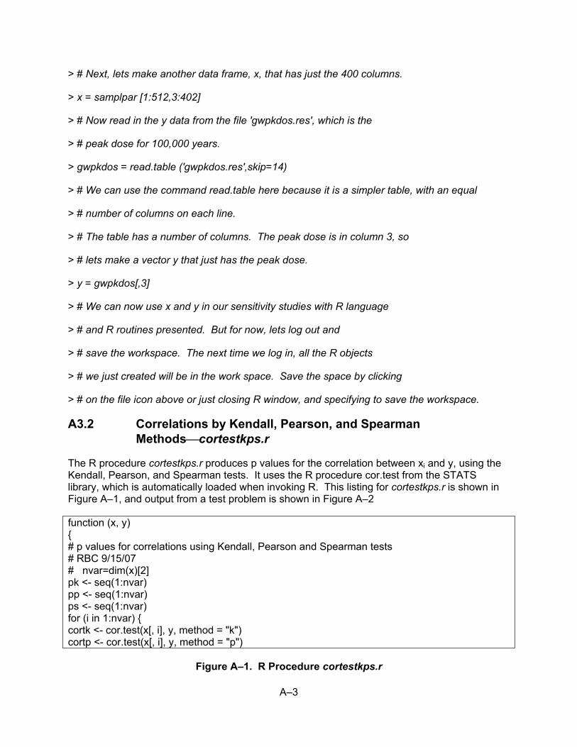
A–3

> # Next, lets make another data frame, x, that has just the 400 columns.

> x = samplpar [1:512,3:402]

> # Now read in the y data from the file 'gwpkdos.res', which is the

> # peak dose for 100,000 years.

> gwpkdos = read.table ('gwpkdos.res',skip=14)

> # We can use the command read.table here because it is a simpler table, with an equal

> # number of columns on each line.

> # The table has a number of columns. The peak dose is in column 3, so

> # lets make a vector y that just has the peak dose.

> y = gwpkdos[,3]

> # We can now use x and y in our sensitivity studies with R language

> # and R routines presented. But for now, lets log out and

> # save the workspace. The next time we log in, all the R objects

> # we just created will be in the work space. Save the space by clicking

> # on the file icon above or just closing R window, and specifying to save the workspace.

A3.2 Correlations by Kendall, Pearson, and Spearman Methods⎯cortestkps.r

The R procedure cortestkps.r produces p values for the correlation between xi and y, using the Kendall, Pearson, and Spearman tests. It uses the R procedure cor.test from the STATS library, which is automatically loaded when invoking R. This listing for cortestkps.r is shown in Figure A–1, and output from a test problem is shown in Figure A–2

function (x, y) { # p values for correlations using Kendall, Pearson and Spearman tests # RBC 9/15/07 # nvar=dim(x)[2] pk <- seq(1:nvar) pp <- seq(1:nvar) ps <- seq(1:nvar) for (i in 1:nvar) { cortk <- cor.test(x[, i], y, method = "k") cortp <- cor.test(x[, i], y, method = "p")

Figure A–1. R Procedure cortestkps.r

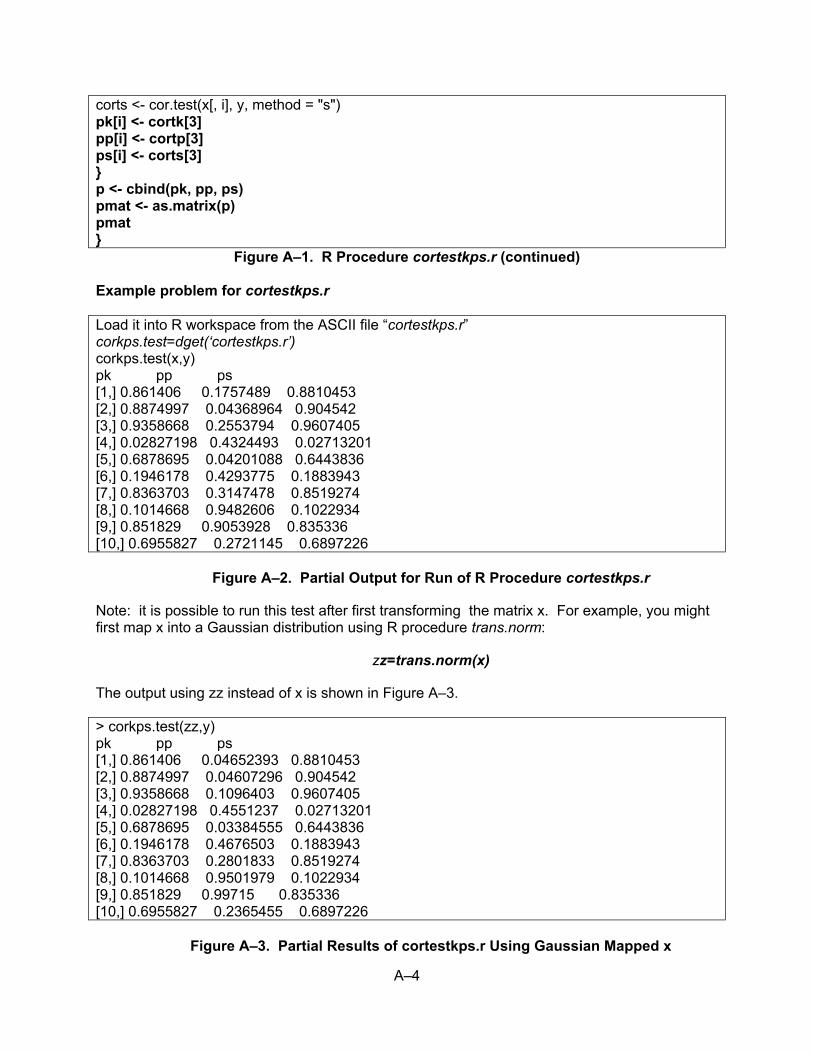
A–4

corts <- cor.test(x[, i], y, method = "s") pk[i] <- cortk[3] pp[i] <- cortp[3] ps[i] <- corts[3] } p <- cbind(pk, pp, ps) pmat <- as.matrix(p) pmat }

Figure A–1. R Procedure cortestkps.r (continued) Example problem for cortestkps.r Load it into R workspace from the ASCII file “cortestkps.r” corkps.test=dget(‘cortestkps.r’) corkps.test(x,y) pk pp ps [1,] 0.861406 0.1757489 0.8810453 [2,] 0.8874997 0.04368964 0.904542 [3,] 0.9358668 0.2553794 0.9607405 [4,] 0.02827198 0.4324493 0.02713201 [5,] 0.6878695 0.04201088 0.6443836 [6,] 0.1946178 0.4293775 0.1883943 [7,] 0.8363703 0.3147478 0.8519274 [8,] 0.1014668 0.9482606 0.1022934 [9,] 0.851829 0.9053928 0.835336 [10,] 0.6955827 0.2721145 0.6897226

Figure A–2. Partial Output for Run of R Procedure cortestkps.r

Note: it is possible to run this test after first transforming the matrix x. For example, you might first map x into a Gaussian distribution using R procedure trans.norm:

zz=trans.norm(x)

The output using zz instead of x is shown in Figure A–3.

> corkps.test(zz,y) pk pp ps [1,] 0.861406 0.04652393 0.8810453 [2,] 0.8874997 0.04607296 0.904542 [3,] 0.9358668 0.1096403 0.9607405 [4,] 0.02827198 0.4551237 0.02713201 [5,] 0.6878695 0.03384555 0.6443836 [6,] 0.1946178 0.4676503 0.1883943 [7,] 0.8363703 0.2801833 0.8519274 [8,] 0.1014668 0.9501979 0.1022934 [9,] 0.851829 0.99715 0.835336 [10,] 0.6955827 0.2365455 0.6897226

Figure A–3. Partial Results of cortestkps.r Using Gaussian Mapped x

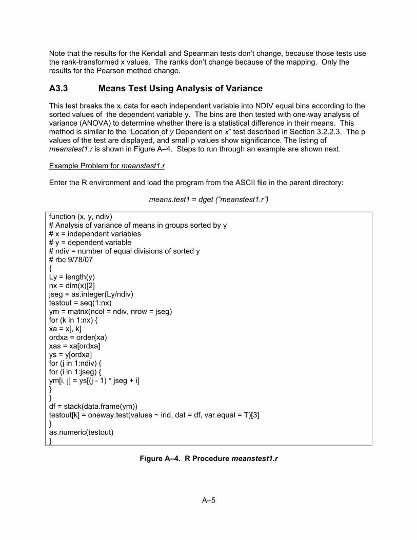
A–5

Note that the results for the Kendall and Spearman tests don’t change, because those tests use the rank-transformed x values. The ranks don’t change because of the mapping. Only the results for the Pearson method change.

A3.3 Means Test Using Analysis of Variance

This test breaks the xi data for each independent variable into NDIV equal bins according to the sorted values of the dependent variable y. The bins are then tested with one-way analysis of variance (ANOVA) to determine whether there is a statistical difference in their means. This method is similar to the “Location of y Dependent on x” test described in Section 3.2.2.3. The p values of the test are displayed, and small p values show significance. The listing of meanstest1.r is shown in Figure A–4. Steps to run through an example are shown next.

Example Problem for meanstest1.r

Enter the R environment and load the program from the ASCII file in the parent directory:

means.test1 = dget (“meanstest1.r”)

function (x, y, ndiv) # Analysis of variance of means in groups sorted by y # x = independent variables # y = dependent variable # ndiv = number of equal divisions of sorted y # rbc 9/78/07 { Ly = length(y) nx = dim(x)[2] jseg = as.integer(Ly/ndiv) testout = seq(1:nx) ym = matrix(ncol = ndiv, nrow = jseg) for (k in 1:nx) { xa = x[, k] ordxa = order(xa) xas = xa[ordxa] ys = y[ordxa] for (j in 1:ndiv) { for (i in 1:jseg) { ym[i, j] = ys[(j - 1) * jseg + i] } } df = stack(data.frame(ym)) testout[k] = oneway.test(values ~ ind, dat = df, var.equal = T)[3] } as.numeric(testout) }

Figure A–4. R Procedure meanstest1.r

A–6

Assuming that x and y are R objects that have been downloaded from samplpar.res and gwpkdos.res and exist in the R environment already, run the means test using three divisions:

means13 = means.test1 (x,y,3)

The object means13 contains the p values for each of the independent variables, which are show here. To quickly find how many values have small p values (e.g., less than 0.05), sort the object means13 (only the first few lines are shown to save space):

> sort(means13)

[1] 0.00095577 0.02707735 0.04085554 0.04541823 0.05855616 0.06737490

[7] 0.08019350 0.09506602 0.09564624 0.10575174 0.11238332 0.11507492

[13] 0.11587876 0.11633140 0.12201281 0.12666697 0.12817294 0.13058053

[19] 0.13058053 0.13082372 0.13524158 0.13914711 0.14680806 0.14823833

In this case, only the first four values of the sorted object have p <0.05. To find out what the variables are, use the order command (just the first few lines are shown):

> order(means13)

[1] 21 23 89 20 50 22 84 3 137 98 38 160 85 131 163 40 178 1

[19] 2 81 93 139 87 130 167 92 162 76 174 122 9 150 140 5 119 110

[37] 42 59 165 53 15 83 41 31 66 12 65 166 172 157 70 120 51 52

[55] 64 80 118 77 113 103 168 169 105 136 30 147 62 155 37 86 63 153

Therefore, the sequence numbers of the variables with p <0.05 in increasing order of p are 21, 23, 89, and 20. A3.4 Wilcoxon Rank Sum Test This is a nonparametric test that is used in this application to determine whether the distribution of the parameter values corresponding to high doses (e.g., X is the top 10 percent of dose values) is different from Y, the total original distribution. The procedure tests the null hypothesis that the means of the two distributions are the same (i.e., μx = μy). If m is the number of samples in the high-dose category X and n the sample size for Y, then the test is conducted by combining the samples from the two populations and ranking the combined sample. The listing for wilcox.r is shown in Figure A–5. Steps to run through an example are shown next.

Example Problem for wilcox.r

In the R environment, download the ASCII file “wilcox.r,” assuming it is in the Windows folder from which R was initiated:

wil.test=dget(‘wilcox.r’)

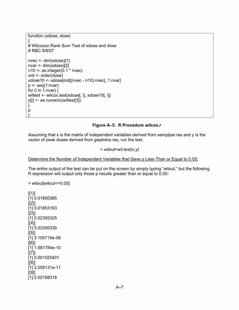
A–7

function (xdose, dose) { # Wilcoxon Rank Sum Test of xdose and dose # RBC 9/8/07 nvec <- dim(xdose)[1] nvar <- dim(xdose)[2] n10 <- as.integer(0.1 * nvec) ord <- order(dose) xdose10 <- xdose[ord[(nvec - n10):nvec], 1:nvar] p <- seq(1:nvar) for (i in 1:nvar) { wiltest <- wilcox.test(xdose[, i], xdose10[, i]) p[i] <- as.numeric(wiltest[3]) } p }

Figure A–5. R Procedure wilcox.r

Assuming that x is the matrix of independent variables derived from samplpar.res and y is the vector of peak doses derived from gwpkdos.res, run the test:

> wilout=wil.test(x,y)

Determine the Number of Independent Variables that Gave p Less Than or Equal to 0.05:

The entire output of the test can be put on the screen by simply typing “wilout,” but the following R expression will output only those p results greater than or equal to 0.05:

> wilout[wilout<=0.05] [[1]] [1] 0.01800385 [[2]] [1] 0.01853163 [[3]] [1] 0.02392325 [[4]] [1] 0.03356339 [[5]] [1] 3.105719e-08 [[6]] [1] 1.581784e-10 [[7]] [1] 0.001925401 [[8]] [1] 2.058131e-11 [[9]] [1] 0.02168318

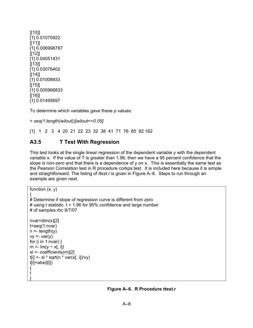
A–8

[[10]] [1] 0.01075922 [[11]] [1] 0.006998787 [[12]] [1] 0.04051431 [[13]] [1] 0.03076402 [[14]] [1] 0.01008933 [[15]] [1] 0.005966833 [[16]] [1] 0.01495697

To determine which variables gave these p values:

> seq(1:length(wilout))[wilout<=0.05]

[1] 1 2 3 4 20 21 22 23 32 38 41 71 76 85 92 162

A3.5 T Test With Regression

This test looks at the single linear regression of the dependent variable y with the dependent variable x. If the value of T is greater than 1.96, then we have a 95 percent confidence that the slope is non-zero and that there is a dependence of y on x. This is essentially the same test as the Pearson Correlation test in R procedure corkps.test. It is included here because it is simple and straightforward. The listing of ttest.r is given in Figure A–6. Steps to run through an example are given next.

function (x, y) { # Determine if slope of regression curve is different from zero # using t statistic. t > 1.96 for 95% confidence and large number # of samples rbc 9/7/07 nvar=dim(x)[2] t=seq(1:nvar) n <- length(y) vy <- var(y) for (i in 1:nvar) { m <- lm(y ~ x[, i]) sl <- coefficients(m)[2] t[i] <- sl * sqrt(n * var(x[, i])/vy) t[i]=abs(t[i]) } t }

Figure A–6. R Procedure ttest.r

A–9

Example Problem for the ttest.r

In the R environment, and assuming that the ASCII file ttest.r is in the working directory or folder, download the function for the t test:

ttest.rbc=dget(“ttest.r”)

Run the t test for y (the peak dose from gwpkdos.res) and x (the independent variables from samplpar.res):

> ttestout=ttest.rbc(x,y)

To determine how many of the tests had t greater or equal to 1.96:

> ttestout[ttestout>=1.96]

[1] 2.017968 2.034265 2.030828 2.627816 4.381198 1.995107 3.816960 2.180037

[9] 1.976501 3.067760 3.144419 2.390151 3.481445 3.382761 3.456404 2.276573

The variable number for t greater than or equal to 1.96 can be found:

> seq(1:length(ttestout))[ttestout>=1.96]

[1] 2 5 15 20 21 22 23 24 38 64 89 92 104 162 166 175 >

A3.6 Stepwise Regression—Forward, Backward, and Akaike Information Criterion Methods

There are three stepwise procedures shown here: stepfor (forward stepwise regression), stepback (backward stepwise regression), and step (forward, backward, or both, using the AIC to iterate on the best fit).

Forward Stepwise Regression⎯stepfor

The R procedures stepfor and stepback are part of the maSigPro library, which must be loaded when R is in its home director with the command:

library(maSigPro)

The stepback command is then invoked and stored in stepbout:

stepbout=stepback(y=y, d=data.frame(x), alfa=0.05)

Arguments of stepfor and stepback

y = The response (e.g., dose from gwpkdos.res)

d = the x matrix as a data frame (e.g., from samplpar.res),

alfa = the alpha value for the hypothesis test.

A–10

The forward stepwise procedure is run exactly the same. R Procedure “step” Using the Akaike Information Criterion (AIC, 2011) The R procedure “step” is part of the STATS library, which is automatically loaded, so you don’t need to invoke the library. Procedure step uses the AIC to assess the value of adding or subtracting a variable, and is more sophisticated than the criteria used in stepfor or stepback. The single parameter of step in its default mode is an lm (linear model) object that describes the fitting equation and the data source:

g=lm(y~. , data=data.frame(x))

This expression says simply that y should be fitted to all variables in the data and that the data are made up of a data frame of x. There are other parameters that can be specified in step. Complete details can be found by using “help(step)” in the R environment. Example Problem for step

stepaic=step(g)

Partial results for an example problem using stepback are given in Figure A–7.

> stepbout=stepback(y=y, d=data.frame(x), alfa=0.05) > summary(stepbout) Call: lm(formula = y ~ ., data = d) Residuals: Min 1Q Median 3Q Max -1.742e-03 -4.185e-04 -5.403e-05 2.758e-04 2.092e-02 Coefficients: Estimate Std. Error t value Pr(>|t|) (Intercept) 3.783e-03 1.763e-03 2.146 0.032357 * X2 1.210e-04 5.172e-05 2.340 0.019655 * X5 -3.216e-03 1.404e-03 -2.290 0.022430 * X15 2.109e-04 1.020e-04 2.067 0.039212 * X21 -1.537e-04 3.144e-05 -4.890 1.37e-06 *** X22 -8.824e-05 4.178e-05 -2.112 0.035183 * X52 3.204e-05 1.552e-05 2.064 0.039553 * X104 1.619e-07 4.886e-08 3.313 0.000991 *** X162 1.702e-04 4.735e-05 3.595 0.000357 *** X166 1.449e-07 3.802e-08 3.812 0.000155 *** X171 3.839e-09 1.695e-09 2.266 0.023898 * X175 9.350e-08 3.585e-08 2.608 0.009388 ** Signif. codes: 0 '***' 0.001 '**' 0.01 '*' 0.05 '.' 0.1 ' ' 1 Residual standard error: 0.001163 on 497 degrees of freedom Multiple R-Squared: 0.2047, Adjusted R-squared: 0.1823 F-statistic: 9.137 on 14 and 497 DF, p-value: < 2.2e-16

Figure A–7. Partial Results From stepback

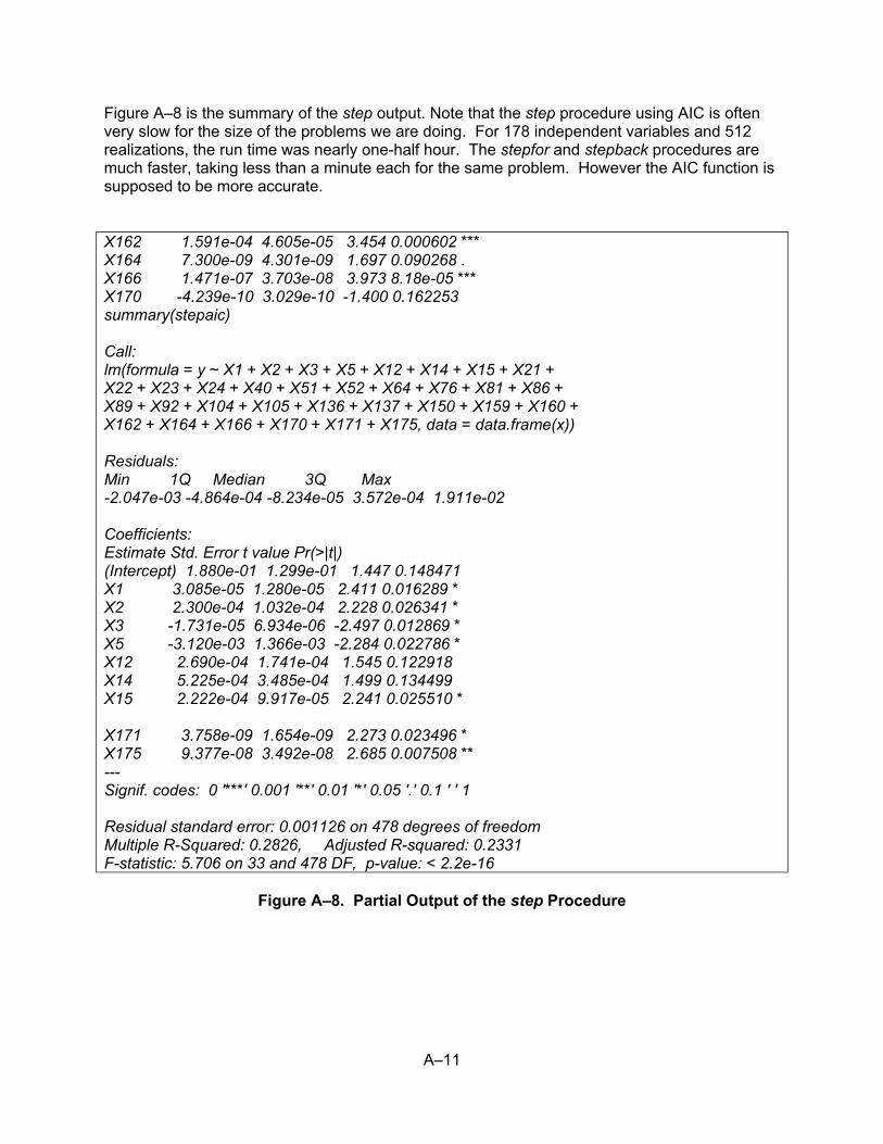
A–11

Figure A–8 is the summary of the step output. Note that the step procedure using AIC is often very slow for the size of the problems we are doing. For 178 independent variables and 512 realizations, the run time was nearly one-half hour. The stepfor and stepback procedures are much faster, taking less than a minute each for the same problem. However the AIC function is supposed to be more accurate. X162 1.591e-04 4.605e-05 3.454 0.000602 *** X164 7.300e-09 4.301e-09 1.697 0.090268 . X166 1.471e-07 3.703e-08 3.973 8.18e-05 *** X170 -4.239e-10 3.029e-10 -1.400 0.162253 summary(stepaic) Call: lm(formula = y ~ X1 + X2 + X3 + X5 + X12 + X14 + X15 + X21 + X22 + X23 + X24 + X40 + X51 + X52 + X64 + X76 + X81 + X86 + X89 + X92 + X104 + X105 + X136 + X137 + X150 + X159 + X160 + X162 + X164 + X166 + X170 + X171 + X175, data = data.frame(x)) Residuals: Min 1Q Median 3Q Max -2.047e-03 -4.864e-04 -8.234e-05 3.572e-04 1.911e-02 Coefficients: Estimate Std. Error t value Pr(>|t|) (Intercept) 1.880e-01 1.299e-01 1.447 0.148471 X1 3.085e-05 1.280e-05 2.411 0.016289 * X2 2.300e-04 1.032e-04 2.228 0.026341 * X3 -1.731e-05 6.934e-06 -2.497 0.012869 * X5 -3.120e-03 1.366e-03 -2.284 0.022786 * X12 2.690e-04 1.741e-04 1.545 0.122918 X14 5.225e-04 3.485e-04 1.499 0.134499 X15 2.222e-04 9.917e-05 2.241 0.025510 * X171 3.758e-09 1.654e-09 2.273 0.023496 * X175 9.377e-08 3.492e-08 2.685 0.007508 ** --- Signif. codes: 0 '***' 0.001 '**' 0.01 '*' 0.05 '.' 0.1 ' ' 1 Residual standard error: 0.001126 on 478 degrees of freedom Multiple R-Squared: 0.2826, Adjusted R-squared: 0.2331 F-statistic: 5.706 on 33 and 478 DF, p-value: < 2.2e-16

Figure A–8. Partial Output of the step Procedure

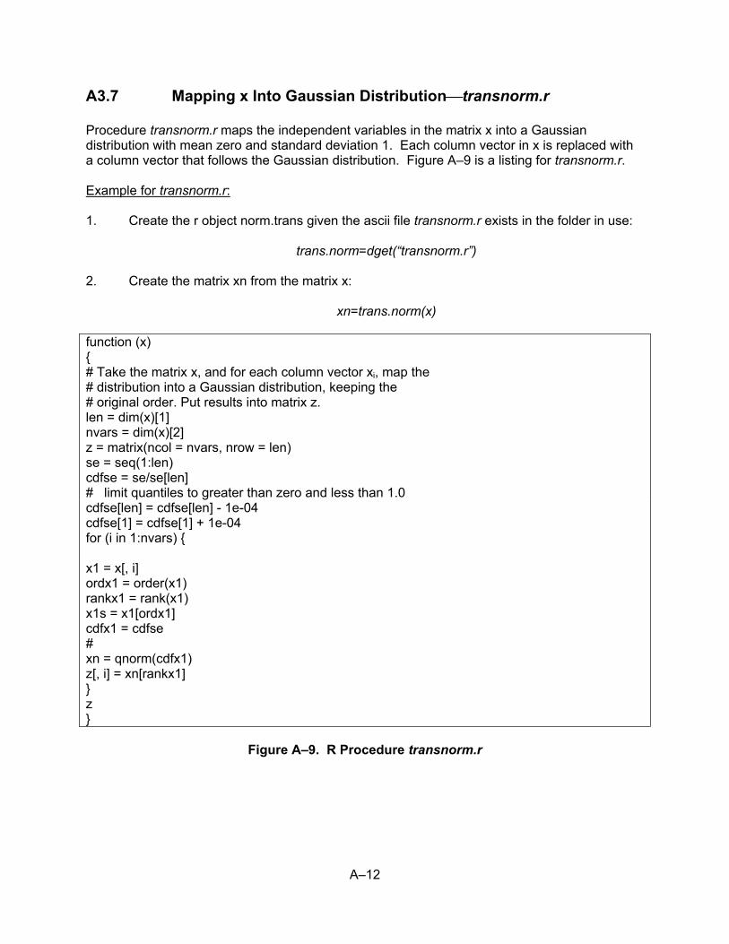
A–12

A3.7 Mapping x Into Gaussian Distribution⎯transnorm.r Procedure transnorm.r maps the independent variables in the matrix x into a Gaussian distribution with mean zero and standard deviation 1. Each column vector in x is replaced with a column vector that follows the Gaussian distribution. Figure A–9 is a listing for transnorm.r. Example for transnorm.r: 1. Create the r object norm.trans given the ascii file transnorm.r exists in the folder in use:

trans.norm=dget(“transnorm.r”)

2. Create the matrix xn from the matrix x:

xn=trans.norm(x)

function (x) { # Take the matrix x, and for each column vector xi, map the # distribution into a Gaussian distribution, keeping the # original order. Put results into matrix z. len = dim(x)[1] nvars = dim(x)[2] z = matrix(ncol = nvars, nrow = len) se = seq(1:len) cdfse = se/se[len] # limit quantiles to greater than zero and less than 1.0 cdfse[len] = cdfse[len] - 1e-04 cdfse[1] = cdfse[1] + 1e-04 for (i in 1:nvars) { x1 = x[, i] ordx1 = order(x1) rankx1 = rank(x1) x1s = x1[ordx1] cdfx1 = cdfse # xn = qnorm(cdfx1) z[, i] = xn[rankx1] } z }

Figure A–9. R Procedure transnorm.r

A–13

A3.8 Transforming x to Its Ranks⎯rankmatrix.r The R procedure rankmatrix.r takes the x matrix and replaces each value with its rank in the columns. Each column is a vector of values for the variable xi. The listing of rankmatrix.r is given in Figure A–10. Example for rankmatrix.r 1. Create the R object rank.matrix given the ascii file rankmatrix.r exists in the folder

in use:

rank.matrix=dget(“rankmatrix.r”)

2. Create the matrix rx from the matrix x:

rx=rank.matrix(x)

function (x) # Input = matrix of x values, nvar column vectors of xi # output = rank replaces values in each column vector xi { nvar <- dim(x)[2] for (i in 1:nvar) { rx[, i] <- rank(x[, i]) } rx }

Figure A–10. R Procedure rankmatrix.r

A4 REFERENCES

Andres, T.H. “Sampling Methods and Sensitivity Analysis for Large Parameter Sets.” Pinawa, Canada: Atomic Energy of Canada Ltd., Whiteshell Laboratories. 2001a. Andres, T.H. “Uncertainty Analysis Guide”. AECL–12103. Pinawa Manitoba : Atomic Energy of Canada Ltd, Whiteshell Laboratories. 2001b. Andres, T.H. “Sampling and Sensitivity Analysis for Large Parameter Sets.” Journal of Statistical Computation and Simulation. Vol. 57. pp 77–110. 1997. CRAN. “Comprehensive R Archive Network.” <http://cran.r-project.org> 2011. Hornick, K. “The R FAQ—Frequently Asked Questions on R.” <http://CRAN.R-Project.org/doc/FAQ/> ISBN3–900051–08–9. 2007. Iman, J. “Stepwise Regression With PRESS and Rank Regression Program User’s Guide.” SAND79–1472. Albuquerque, New Mexico: Sandia National Laboratories. 1980.

A–14

Kleijnen, P.C. and J.C. Helton. “Statistical Analyses of Scatterplots To Identify Important Factors in Large-Scale Simulations.” SAND–98–2202. Albuquerque, New Mexico: Sandia National Laboratories. April 1999. MathSoft, Inc. “STATSCI—S-Plus Reference Manual.” Seattle, Washington: MathSoft, Inc., StatSci Division. 1993. Shortencarier, M. and J. Helton. “A FORTRAN 77 Program and User’s Guide for the Statistical Analyses of Scatterplots To Identify Important Factors in Large-Scale Simulations.” SAND99–1058. Albuquerque, New Mexico: Sandia National Laboratories. 1999.