history is a mirror to the future: best-effort approximate ... · history is a mirror to the...
TRANSCRIPT

History is a mirror to the future: Best-effort approximatecomplex event matching with insufficient resources
Zheng LiOracle Corporation
Tingjian GeUniversity of Massachusetts, Lowell
ABSTRACTComplex event processing (CEP) has proven to be a highlyrelevant topic in practice. As it is sensitive to both errorsin the stream and uncertainty in the pattern, approximatecomplex event processing (ACEP) is an important direc-tion but has not been adequately studied before. ACEP iscostly, and is often performed under insufficient computingresources. We propose an algorithm that learns from thepast behavior of ACEP runs, and makes decisions on whatto process first in an online manner, so as to maximize thenumber of full matches found. In addition, we devise effec-tive optimization techniques. Finally, we propose a mecha-nism that uses reinforcement learning to dynamically updatethe history structure without incurring much overhead. Puttogether, these techniques drastically improve the fractionof full matches found in resource constrained environments.
1. INTRODUCTIONComplex event processing has proven to be useful in prac-
tice. Complex event matching is sensitive to both errorsin data streams and errors or uncertainty in patterns. Acomplex event pattern p is usually represented as a regularexpression extended with a window constraint, allowing in-terleaving of irrelevant events [5, 9]. Thus, when there is onecritical basic event in the stream sequence that is supposedto match a basic event in p but differs due to noise or missingevents, then the match will fail altogether. Furthermore, auser who issues the complex event query may not always beexactly sure about the pattern p. She roughly knows whatshe is looking for, and tries to specify a pattern p. However,if a piece of the stream matches p approximately, it mightbe an interesting match. Let us look at an example.
Example 1. Twitter is one of the most popular socialnetworks. We can define basic events (i.e., letters), as wellas complex event patterns to find complex events of interestin a timely fashion from the Twitter stream. For instance,suppose we want to detect “buy” or “sell” points for the com-pany Apple’s stock. The idea is that if there are discussionsof bullish stock chart patterns, followed by some good news
This work is licensed under the Creative Commons Attribution-NonCommercial-NoDerivatives 4.0 International License. To view a copyof this license, visit http://creativecommons.org/licenses/by-nc-nd/4.0/. Forany use beyond those covered by this license, obtain permission by [email protected] of the VLDB Endowment, Vol. 10, No. 4Copyright 2016 VLDB Endowment 2150-8097/16/12.
of the company, we identify it as a buy point (as the stockwill likely go up). We can use the following pattern:
p = [Sa(b|d|w|r)E]2+[Sa(g|e|u)E]2+ (1)
where S is the start of a tweet (identified by @name in thetext), E is the end of a tweet (identified by a timestamp),a is the appearance of stock symbol $AAPL (Apple, Inc.), bis “bullish”, d is “double bottom”, w is “falling wedge”, r is“rounding bottom”, g is “decent/solid guidance”, e is “goodearnings”, and u is “upgrade”. Note that d, w, and r aretypical bullish stock chart patterns (more can be included)signifying a potential upward movement of the company’sstock price in the future, while g, e, and u are typical goodnews of a company that ensures the upward movement (theseterms are usually posted by experienced traders or tradingprofessionals). The notation “2+” means the pattern in thebrackets occurs two or more times. Thus, p finds two ormore tweets that indicate a potential upward trend followedby two or more tweets that corroborate it with good news evi-dence. The whole pattern indicates a “buy” point for Apple.
In Example 1, similarly we can define a complex event fora “sell” point and do this for many companies. Here, the ba-sic events/letters are derived from matching keywords, andthe timestamp of a letter is the timestamp of the correspond-ing tweet. There is clearly uncertainty in the letter sequencesince a trader may not use a term that we expect. We arenot completely sure about the pattern p; a little deviationfrom it is probably a good discovery too. We study approxi-mate complex event processing (ACEP). Our semantics is arelaxation of the commonly-used exact version by allowingat most k event errors in the match instance. For instance,in Example 1, we may have k = 1 which allows at most onemismatch of the required letters.
Complex event processing can be very resource consum-ing, as every intermediate matching state has to be kept inthe system until either it results in a full match or the matchwindow expires. This process is also nondeterministic, forwe want to get all match instances—the actions of movingto the next state (due to a letter match) and staying in thecurrent state are both valid. ACEP makes it even morenondeterministic, since we now also have the choice to skipa letter and go to the next state, adding one to the error.The performance issue is a showstopper when the processingspeed cannot keep up with the stream rate.
The aforementioned problem is even more serious if weconsider a novel application where more computing is pusheddown to endpoint small devices such as smartphones, inorder to reduce the amount of communicated data to theserver. In particular, an application may want to perform
397
such ACEP matching in situ—on smartphones or other de-vices with limited computing power. Only matched instancesare communicated to the remote server. Hence, it is imper-ative to study resource-constrained ACEP (RC-ACEP).
RC-ACEP is a best-effort attempt to discover as many oc-currences of the searched patterns as possible, given that thestream rate is higher than can be handled by available com-puting resources. For RC-ACEP, we propose a novel learn-ing method using a data structure H we build for the recentmatch history. We look up H to determine which interme-diate partial matching states are more likely to eventuallyend up with a full match. We devise an online algorithm andprove its competitive ratio. Furthermore, we propose an op-timization technique called proxy match, and devise a novelsketch technique to further reduce the memory consump-tion. Finally, we use a reinforcement learning technique todynamically update H with little overhead. Our contribu-tions are summarized below:
• We propose the ACEP problem and devise an algo-rithm for it (Sections 2 and 3.1).
• We study the RC-ACEP problem, and propose a novelalgorithm that learns from history. (Section 3.2).
• We devise an optimization called proxy match, and ahistory sketch with its analysis (Sections 3.3 and 4).
• We propose dynamic update of the history structurebased on reinforcement learning (Section 5).
• We perform a systematic experimental evaluation us-ing two real world datasets (Section 6).
2. PROBLEM FORMULATIONWe are given a sequence s = s[1], s[2], ... where each char-
acter s[i] is in Σ, the alphabet. We use the terms sequenceand stream interchangeably, and use character, letter, andevent interchangeably. Each s[i] has a tag t[i]. If t[i] is thetimestamp when s[i] is generated, we get time-window se-mantics. If t[i] is a counter (i.e., t[i] = i), we get count-window semantics. The sequence s has increasing tags.Without loss of generality, we assume time windows. Asubsequence is a sequence that can be derived from anothersequence by deleting some letters without changing the orderof the remaining letters. For example, the sequence “bde”is a subsequence of “abcdef”.
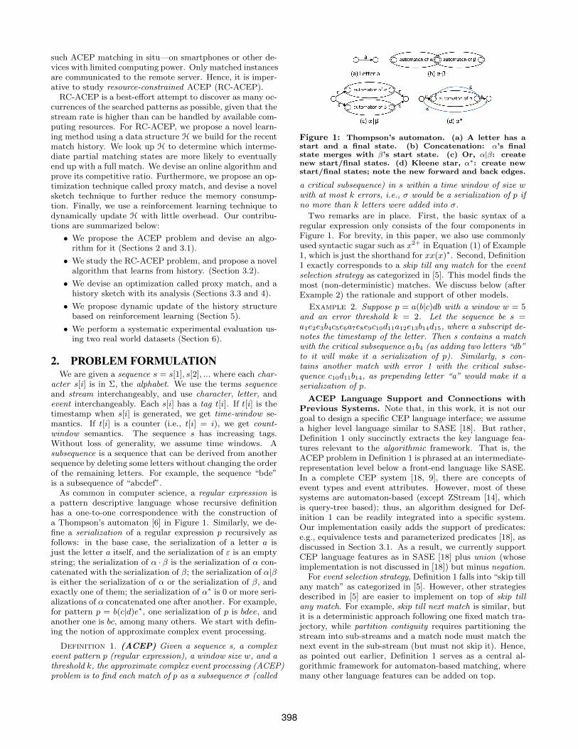
As common in computer science, a regular expression isa pattern descriptive language whose recursive definitionhas a one-to-one correspondence with the construction ofa Thompson’s automaton [6] in Figure 1. Similarly, we de-fine a serialization of a regular expression p recursively asfollows: in the base case, the serialization of a letter a isjust the letter a itself, and the serialization of ε is an emptystring; the serialization of α · β is the serialization of α con-catenated with the serialization of β; the serialization of α|βis either the serialization of α or the serialization of β, andexactly one of them; the serialization of α∗ is 0 or more seri-alizations of α concatenated one after another. For example,for pattern p = b(c|d)e∗, one serialization of p is bdee, andanother one is bc, among many others. We start with defin-ing the notion of approximate complex event processing.
Definition 1. (ACEP) Given a sequence s, a complexevent pattern p (regular expression), a window size w, and athreshold k, the approximate complex event processing (ACEP)problem is to find each match of p as a subsequence σ (called
Figure 1: Thompson’s automaton. (a) A letter has astart and a final state. (b) Concatenation: α’s finalstate merges with β’s start state. (c) Or, α|β: createnew start/final states. (d) Kleene star, α∗: create newstart/final states; note the new forward and back edges.
a critical subsequence) in s within a time window of size wwith at most k errors, i.e., σ would be a serialization of p ifno more than k letters were added into σ.
Two remarks are in place. First, the basic syntax of aregular expression only consists of the four components inFigure 1. For brevity, in this paper, we also use commonlyused syntactic sugar such as x2+ in Equation (1) of Example1, which is just the shorthand for xx(x)∗. Second, Definition1 exactly corresponds to a skip till any match for the eventselection strategy as categorized in [5]. This model finds themost (non-deterministic) matches. We discuss below (afterExample 2) the rationale and support of other models.
Example 2. Suppose p = a(b|c)db with a window w = 5and an error threshold k = 2. Let the sequence be s =a1e2e3b4c5e6a7e8e9c10d11a12e13b14d15, where a subscript de-notes the timestamp of the letter. Then s contains a matchwith the critical subsequence a1b4 (as adding two letters “db”to it will make it a serialization of p). Similarly, s con-tains another match with error 1 with the critical subse-quence c10d11b14, as prepending letter “a” would make it aserialization of p.
ACEP Language Support and Connections withPrevious Systems. Note that, in this work, it is not ourgoal to design a specific CEP language interface; we assumea higher level language similar to SASE [18]. But rather,Definition 1 only succinctly extracts the key language fea-tures relevant to the algorithmic framework. That is, theACEP problem in Definition 1 is phrased at an intermediate-representation level below a front-end language like SASE.In a complete CEP system [18, 9], there are concepts ofevent types and event attributes. However, most of thesesystems are automaton-based (except ZStream [14], whichis query-tree based); thus, an algorithm designed for Def-inition 1 can be readily integrated into a specific system.Our implementation easily adds the support of predicates:e.g., equivalence tests and parameterized predicates [18], asdiscussed in Section 3.1. As a result, we currently supportCEP language features as in SASE [18] plus union (whoseimplementation is not discussed in [18]) but minus negation.
For event selection strategy, Definition 1 falls into “skip tillany match” as categorized in [5]. However, other strategiesdescribed in [5] are easier to implement on top of skip tillany match. For example, skip till next match is similar, butit is a deterministic approach following one fixed match tra-jectory, while partition contiguity requires partitioning thestream into sub-streams and a match node must match thenext event in the sub-stream (but must not skip it). Hence,as pointed out earlier, Definition 1 serves as a central al-gorithmic framework for automaton-based matching, wheremany other language features can be added on top.
398

We note that there are richer CEP language features suchas negation (which can be added on top of ours), those inSASE+ [5] regarding more complex predicates and HAVINGclauses, and the hierarchical structures in XSeq [15]. How-ever, as pointed out earlier, the algorithmic frameworks inthe previous work are almost all automaton-based (exceptZStream [14] which is query-tree based). Even XSeq is basedon the Visibly Pushdown Automata, a generalization of fi-nite state automata [15]. Thus, the main contributions ofour paper, including using a history structure over the matchnodes at automaton states to perform resource-constrainedmatching, can be easily adopted for a particular instance ofCEP system and language. ZSream supports conjunction[14], which can be added on top of an automaton-based al-gorithmic framework too, as done in [13]. An interestingpoint raised in ZStream [14] is that it is beneficial to havea flexible (rather than fixed) evaluation order. This indeedcan be accomplished in an automaton-based framework too,as done in the automaton sketch optimization in [13]. Poten-tially, our history-based resource-constrained matching canbe adopted for a tree-based framework like ZStream as well,where the history would contain tree nodes; we leave this asfuture work. An extensive survey of CEP language featuresis beyond the scope of this paper, and we refer the readerto an excellent survey paper [9].
Finally, regarding error metric, edit distance [16] is oftenused as the distance metric between two sequences, in whicha unit cost is inflicted for each insertion, deletion, or updateof a letter. However, in our case (a match between a patternand a stream window), for the skip till any/next match, theabove three operations can be merged to one: an insertionto the stream. This is because update of a letter to thestream is the same as insertion, and deletion is free (due tothe skips). For other models that require contiguity (i.e.,substring rather than subsequence match), edit distance canbe used. A potential generalization of our error model is togive weights to each inserted letter that would form a serial-ization of the pattern, as missing events may have differentlevels of importance. This is particularly the case if we addnegations to the patterns, because the presence of a negativeevent in the stream may get far more penalty than missinga positive event. We now define RC-ACEP.
Definition 2. (RC-ACEP) The resource constrained ap-proximate complex event processing (RC-ACEP) problem isthe ACEP problem under actual computing resources, withthe requirement of giving answers online. Specifically, thereis a time constraint determined by the dynamic data streamrate. The online processing must keep up with the streamrate, and return as many matches as possible.
We focus on the time constraints (i.e., insufficient com-puting time), although in one variation of our solution wealso significantly reduce memory consumption by building asketch of our data structure. We first present an algorithmfor ACEP ignoring resource limits (i.e., the online require-ment). Then we concentrate on the RC-ACEP problem.
3. ACEP AND RC-ACEP ALGORITHMS3.1 ACEP Algorithm
We first devise ACEPMatch that does the matching with-out considering the online requirement. We use a Thomp-son’s automaton [6], whose recursive construction is illus-trated in Figure 1. A state can either be an L-state (with
only one incoming letter edge) or an ε-state (with one ormore incoming ε edges). There is a correspondence betweenany regular expression p and such an automaton; thus ACEPuses such an automaton as the input pattern. A central con-cept of ACEP is match trajectory, which consists of a numberof match nodes, and indicates a specific critical subsequencein s that causes the match of p. A match node is a tuple:
(state, loc, err, start win, prev state, prev loc, prev err)
where state is the current automaton state, loc is the loca-tion (index) of the letter in the stream s that matches thisL-state (if any), err is the error (number of mismatches),start win is the start time of this window, prev state is theprevious L-state that is matched to the letter at prev locin the stream with an error prev err. The prev ∗ fields areused to chain the match nodes into a match trajectory. Thematching algorithm basically keeps tracks of linked matchnodes located at each state of the automaton. When oneof them is at a final state, the whole match trajectory canbe retrieved by following the links backwards. Match nodesexpire when they are out of the current window.
Algorithm 1: ACEPMatch(s,A, k)
Input: s: incoming stream, A: automaton for pattern p, k:error threshold
Output: match trajectories1 seed← (start{A}, null, 0, null, null, null, 0)2 propagate(seed,A, k) //Pre-compute this only once3 for each incoming letter s[i] in s do4 for each L-state σ of A that matches s[i] do5 for each match node µ at a state in pre(σ) do6 if µ.start win = null then7 start win← t[i]8 else9 start win← µ.start win
10 if µ.loc = null then11 prev ∗ ← µ.prev ∗12 else13 prev ∗ ← µ.∗14 err ← µ.err15 create λ← (σ, i, err, start win, prev ∗) at σ16 propagate(λ,A, k)17 if any match node at final state then18 report it
1 Procedure propagate(µ,A, k)2 for each state σ ∈ post(µ.state) in A do3 if σ is L-state then4 err ← µ.err + 15 else6 err ← µ.err
7 if err > k then8 continue;
9 if µ.loc = null then10 prev ∗ ← µ.prev ∗11 else12 prev ∗ ← µ.∗13 create λ← (σ, null, err, µ.start win, prev ∗) at σ14 propagate(λ,A, k)
In line 1 of ACEPMatch, we create a single “seed” matchnode at the start state of the automaton, start{A}, with er-ror 0 and other fields null (the format of a match node isshown earlier). All other match nodes later created duringthe algorithm are descendants of this single seed. Note that
399

the start state is an ε-state, which is why it does not con-sume any input letter for the seed to be on. For an L-statewith incoming letter l, a match node can be on it only afterconsuming a letter l from the stream, or after skipping theletter l (with an additional error 1 incurred).
Line 2 calls the propagate procedure to propagate andderive new match nodes from the seed. This is to skip up tok L-states (each incurring error 1) and generate new matchnodes. Line 2 of the propagate iterates through each poststate (i.e., a state that immediately follows the current state)and tries to generate a new match node based on the originalone. An error 1 is incurred if the new state is an L-state. Inlines 9-12 of propagate, it first checks if µ’s stream locationis null. If so, it is not an L-state match there, and hencethe prev ∗ fields (i.e., prev state, prev loc, and prev err)of the new match node (created in line 13) should be takenfrom µ’s prev ∗ fields (line 10). Otherwise there is an L-state match at µ, and we set the new prev ∗ fields to µ’scorresponding fields (state, loc, err) (line 12). Finally, inline 14 of propagate, the procedure is recursively called overthe new match node until it cannot be propagated further(either when error is over k or at a final state).
Lines 3-4 of ACEPMatch iterate through each letter s[i]and each L-state σ that matches the letter. This matchwill trigger the creation of a new match node at σ (line 15).Such a new match node is based on an existing match nodeµ at a previous state in line 5, where pre(σ) denotes the setof states that immediately precede state σ. Note that if amatch node µ in line 5 has expired, it is simply removed.Lines 10-13 are to set the prev ∗ fields of this new matchnode (same as lines 9-12 of propagate).
Example 3. As in Example 2, let p = a(b|c)db, w = 5,k = 2, and the automaton is shown in the top plot of Fig-ure 2, where S1 is the start state and S6 is the final state.The bottom plot illustrates ACEPMatch, where a matchnode is simplified as a two-value tuple only (state and er-ror). Stream events with timestamps as subscript are shownvertically (c1d2a3e4b5). (S1, 0) is the seed node before anyevents arrive, with error 0. Line 2 of ACEPMatch propa-gates the seed to the three match nodes to the right of it in thesame row. When c arrives at time 1, the matching L-stateS4 is examined (line 4) whose pre set only has S2. Thus, anew match node (S4, 1) is created based on (S2, 1). A solidarrow indicates such a “match and advance” action, corre-sponding to (the reverse of) the prev ∗ chain pointers, whilea dashed arrow indicates skipping a letter during propagate.The red arrows together form a match trajectory with error1 at time 5. The blue arrows form another match trajectorywith error 2. This example shows that there can be manyvery similar match trajectories. Our subsequent techniques(Sections 3.2 and 3.3) will address this issue.
Note that we easily support predicates for the higher levellanguage SASE [18], which is not shown in ACEPMatchfor clarity. For a predicate that involves a number of eventvariables X1, ..., Xc, whenever an event variable is matched,we record the attribute value in the match node. Whenthe last event among the c events is matched, we check thepredicate and do not form a new match node if the pred-icate is false. For instance, suppose we have a predicateD.att1 > A.att2 in the pattern of Figure 2, where D and Aare the event types/variables of d and a, respectively. Thenwe record A.att2 in a match node and evaluate the predicate
Figure 2: An automaton and the ACEP matching al-gorithm. We show two of the match trajectories, one inred and the other in blue. A solid edge indicates a lettermatch, and a dashed edge is a propagation with error.
when a match is triggered in state S5. This is analogous tothe “predicate pushdown” optimization in [18].
Connection with SASE [18]. Both ACEPMatch andSASE matching use an NFA. We next show that there isan interesting connection between the two: When the errorthreshold k is 0, ACEPMatch is the same algorithm as theSASE along with all the optimizations presented in [18], plusthe union support, and minus the negation support. We ob-serve that there is a one-to-one correspondence between thesupported features/algorithm components of SASE (withthe optimizations in [18]) and ACEPMatch when k = 0.The Sequence Scan and Construction (SSC) using ActiveInstance Stack (AIS) (presented in Section 4.1 and Figure 3of [18]) is algorithmically equivalent to our match nodes andmatch trajectories. Specifically, an element in the AIS asso-ciated with an automaton stack corresponds to our matchnode, while an arrow/pointer in Figure 3 of [18] correspondsto our prev ∗ pointers used to trace back the match trajecto-ries. When k = 0, the propagate procedure in ACEPMatchwill never propagate a match node to a following L-state asthere is no error budget and propagate does not consumeany event—thus SASE and ACEPMatch progress amongthe states in the same manner and complexity.
Earlier we have discussed how our algorithm handles pred-icates. Our framework does the same “pushing an equiva-lence test down” optimization (Partitioned Active InstanceStacks in Section 4.2.1 of [18]) by running an instance ofACEPMatch for each partitioned sub-stream. The cross-attribute transition filtering in Section 4.2.2 [18] correspondsto our discussion above where a predicate is evaluated whenthe last event type in the pattern is matched. Moreover,ACEPMatch does the “pushing windows down” optimiza-tion in Section 4.3 of [18], as it keeps track of the start ofa window in each match node, which is removed when thewindow expires. In all, we have the algorithmic equivalenceas stated earlier. Of course, the design of ACEPMatch isfor the main goal of approximate match when k 6= 0.
3.2 History and RC-ACEPAs discussed earlier, ACEP can easily exceed resource lim-
its. We now present the RC-ACEP algorithm that does thebest-effort most-profitable online processing. The basic ideais that we can somehow compactly represent a history ofpast run into a data structure H. At runtime, based on H,
400

we discard some match nodes that are unlikely to result ina final full match. However, this is not a straightforwardproblem where we can apply an off-the-shelf machine learn-ing technique. We illustrate this point below.
At any moment, there are many active match nodes thatare ready to be expanded. A match node may wait at anautomaton state, or it can skip to a subsequent state butincur an error, or it can simply be discarded. When thereis a letter match, there may also be a choice whether to ad-vance into a union branch or not. Hence, there are manychoices/decisions to make. Letting each match node inde-pendently decide what choice to make would not work wellas a whole. This is because they are heavily correlated—asequence of future events in the stream may make multiplematch nodes to complete a full match together (in the sametime window) or mutually exclusively.
One example is the match nodes at the same or nearby au-tomaton states. There are slight variations of essentially thesame matches. For instance, two matches may differ onlyby one letter or by one error. The correlation between twomatch trajectories is caused by the same set of close eventsthat occur in the stream. The key insight is that, if twomatch trajectories are within the same window (or close by),we only need to keep one match node and discover one of thetrajectories. It is more important to detect which time win-dow has the match; this is often sufficient already, especiallygiven the minor differences among the trajectories. Oncewe locate the window, if we really needed to enumerate alltrajectories, we could simply do so for that stream windowonly—which incurs significantly less cost than maintainingall match trajectories throughout their lifetimes. Thus, fromH, we learn if two match nodes tend to produce match tra-jectories that are in the same window or close together, sothat we only keep one of them.
Definition 3. (Match Point, Match Bundle) The time(tag) of the last event in the stream s that matches an L-state in p and completes a match trajectory τ (i.e., reportedin line 18 of ACEPMatch) is called a match point of τ ,denoted as m(τ). A match bundle is a set T of match tra-jectories such that: (1) (Proximity) if |T | > 1, then ∀τ ∈T,∃τ ′ ∈ T, τ ′ 6= τ, |m(τ)−m(τ ′)| ≤ w; (2) (Maximality) T ismaximal in that ∀τ ∈ T,∀τ ′, |m(τ)−m(τ ′)| ≤ w ⇒ τ ′ ∈ T .
The above definition indicates that a match bundle con-tains a contiguous region of match points that spans anarbitrary time interval. The proximity property says thateach match point has at least another one that is close (un-less the whole bundle has only one match point), while themaximality property says that the bundle cannot be furtherexpanded on either side in time. Thus, any two match bun-dles in a stream are non-overlapping; otherwise they wouldbe merged into one.
Example 4. In Figure 2 (Example 3), the upper matchtrajectory (red) has a match point of 5, which is the times-tamp of the last event b5 that triggers its last L-state match.Similarly, the lower match trajectory (blue) also has a matchpoint of 5. These two match trajectories are in the samematch bundle, as the distance between their match pointsare clearly within w.
All match trajectories in a stream are partitioned into dis-tinct match bundles. Intuitively, a match bundle indicatesan area in the stream that contains matches. Once we locatea match point t anywhere in a match bundle, if all match
Figure 3: Illustrating the history data structure H.Each green box is a match vector type of vertex, andeach red ball is a match bundle type of vertex, occurringduring some time interval in the stream.
trajectories were to be retrieved, we could extend t on bothsides of the stream (forward and backward) by w at a time,and do a match in the local area of t until an extension re-sulted in no more matches. By the definition of a matchbundle, it is easy to see that two closely correlated matchnodes (that tend to either both succeed or both fail to leadto a full match—due to the chance in event sequence) willalso tend to lead to the same match bundles in the historyH. Hence, match bundles are a crucial part of a history.
Definition 4. (History) A history H for a time inter-val [t1, t2] is a directed graph with vertex labels. H has twotypes of vertices: (1) a match vector (state, remaining w, err,time since last), where state is the current state in the au-tomaton, remaining w is the remaining window size, err isthe currently incurred match error, and time since last isthe time since the last event match within a match trajectory,and (2) a match bundle. In addition, a match vector vertexis also labeled with an integer count of visits, while a matchbundle vertex is labeled with its ID (unique in the stream).An edge between two match vectors indicates a visit sequencefrom one to the other, while an edge from a match vector toa match bundle indicates that the match vector directly leadsto the match bundle.
Example 5. Figure 3 illustrates the history data struc-ture H learned from a period of run of the pattern in Ex-ample 2. The green rectangles are type (1) vertices in Def-inition 4—match vectors, while the red balls at the bottomlevel are type (2) vertices—match bundles in time order ofthe stream. A match vector is essentially a state of a par-ticular match node (remaining w and time since last arediscretized into integers for various interval sizes in a win-dow), and the count is the number of times reaching thatvector state during the period of run. Many vertices areomitted from the figure. Note that some match vectors maynot have outgoing edges, corresponding to the expiration ofthe match node without full matches. Moreover, one matchbundle may have incoming edges from multiple match vec-tors, indicating that those match vectors are correlated andhad match instances in the same match bundle in the stream.
A common operation we will perform on H is to lookup the list of match bundles reachable from a given matchvector. Thus, for fast lookup, we associate with each matchvector vertex a bitmap called a match map. A match mapis a bitmap with one bit for each match bundle in H. A bitis set to 1 if the corresponding match bundle is reachablefrom that match vector. For example, in Figure 3, everymatch vector node has a bitmap (match map) of 6 bits. Thematch map at the match vector (S5, 3, 2, 1) has a match map
401

011010, as it has b2, b3, and b5 as descendants. The H hereis small for clarity. In a real structure, typically each matchmap has hundreds or thousands of bits.
H can be easily built while we run the ACEP matchingalgorithm on the data stream. As each match vector state isencountered, we increment its count in H . Whenever thereis a full match, we trace back the match trajectory and setbit 1 for the corresponding match bundle in each match mapof the match vector node on the trajectory.
Given a history H, we solve the RC-ACEP problem. Thebasic idea is as follows. We must pick more “promising”match nodes and process them first. This is done in anonline manner such that, when the next stream event arrives(before we finish processing all match nodes), we stop andprocess this new stream event. Thus, the question becomes:given a set of currently active match vectors, which onesshould we pick in an online manner so that the number offull matches can be maximized? H shows the set of matchbundles each active match vector led to in the past, throughthe match map at that match vector.
Intuitively, this problem can be reduced to a variant of themaximum coverage problem [11]. Recall that the maximumcoverage problem is: One is given several sets and a numberθ; the sets may have some elements in common. One mustselect at most θ of these sets such that the maximum numberof elements are covered. In RC-ACEP, upon each streamevent, each active match vector maps to a set, where eachelement in a set is a match bundle in H. Since we cannothandle all the active match vectors, we want to pick a limitednumber of them so that they cover as many match bundlesin H as possible.
However, there are two major differences: (1) In the max-imum coverage problem, we get to pick a fixed number (θ)of sets to maximize the number of elements covered. In RC-ACEP, due to the highly dynamic nature of stream rates andsystem resource environment, we do not know in advancehow many match vectors we can finish. We must processthem in an online manner. (2) The match map statistics ateach match vector in H is biased by its visit count. Thatis, if vector v1 is visited less often in history than vector v2,it tends to have fewer “1” bits (i.e., match bundles) in itsmatch map. But given the fact that they are both activeat the current moment, we should remove this bias and usethe statistics conditioning on the fact that are both active.
For instance, in Figure 3, suppose at present two matchvectors v1(Cnt = 29) and v2(Cnt = 42) are active. Thenwe normalize v1’s match bundle counts by multiplying themwith 42/29 = 1.45. That is, choosing v1 covers b1 and b31.45 times, while choosing v2 covers b2, b3, and b5 1 time.Choosing both still covers b3 1.45 times (multiset union).Thus, our solution generalizes sets to multisets in the max-imum coverage problem.
The algorithm is shown in Algorithm 2. We say that aletter is a matching letter if it matches at least one L-statein the automaton. Lines 1-2 are the same as ACEPMatch,setting up the seed match nodes. In line 3, we use the key-word “immediately”, meaning that whenever a new match-ing letter arrives, we must stop the block of code below line3 (even if it is not finished), and process this new letter.Line 4 initializes an array max[.] to all 0’s. The size of thisarray is the same as the number of bits in a match vector.It is used to keep track of the maximum number of times amatch bundle has been covered so far.
Lines 5-11 iterate through each match node at the “pre”state of each L-state that matches the incoming letter. Thesematch nodes are candidates. We will later pick and processthem one by one until time is out and the next letter arrives.In line 7, we look up H and get the match node’s match vec-tor’s information: number of visits and match map. Line 8is to get the multiplicity of each bundle covered by µ as dis-cussed above. z is a scale constant that can be set to anyvalue (e.g., maximum count, for numerical accuracy). Inline 9, 1(b) denotes the number of 1’s in bitmap b; with mul-tiplicity, score is the initial total count of bundle coverage.
Algorithm 2: RC-ACEP(s,A, k,H)
Input: s: incoming stream, A: automaton for pattern p, k:error threshold, H: history
Output: match trajectories1 seed← (start{A}, null, 0, null, null, null, 0)2 propagate(seed,A, k)//Pre-compute this only once3 for each arriving matching letter s[i] immediately do4 reset max[.]5 for each L-state σ of A that matches s[i] do6 for each match node µ at state pre(σ) do7 get µ’s count c and match map b from H8 m← z
c//z is a constant; m is multiplicity
9 score← 1(b)×m10 global version← 111 put (µ,m, b, global version, score) into priority
queue Q with priority score
12 while Q is not empty do13 (µ,m, b, version, score)← pop maximum from Q14 updates← look up version table using version15 if updates & b 6= 0 then16 score←
∑i∈bmax(m−max[i], 0)
17 put (µ,m, b, global version, score) back to Q
18 else19 process µ as in ACEPMatch lines 6-1820 update max[.], global version, version table
The algorithm uses a simple version table, which is justan array associating a version number (starting from 1) witha bitmap of updates in max[] since that version. This is toefficiently keep track of whether scores are up to date duringthe greedy selection of match nodes. Lines 10-11 put theinitial version of match nodes into a heap (priority queue).Lines 13-15 get the maximum score match node µ from theheap, and look up the positions of updates in max[.] sinceits version. If they overlap µ’s match map b, in line 16, weupdate µ’s score to a smaller one, removing the counts ofmatch bundles already covered since the previous version.Otherwise, in line 20, we update max[.] for newly coveredbundle counts, increment the global version, and updatethe update-maps of the version table.
Overall, lines 4-20 are a novel integration of the onlinegreedy maximum coverage algorithm and an A*-style search[12]. The goal is to pick which match vectors to process in anonline manner to maximize the total (normalized) count ofmatch bundles covered by the selected match vectors. TheA* search in particular is to efficiently search for a matchvector that gives the maximum coverage increment of matchbundles. Thus, the negative value of the score of each activematch node is regarded as the f cost function in the stan-dard A* model [12], where score is the coverage incrementsince any version (as recorded in Q). It is the sum of two
402

cost functions (g and h in the A* model), where g corre-sponds to the coverage increment since global version, andh corresponds to the coverage between the version recordedin Q and global version. Thus, score is always an upperbound of the true increment, and the algorithm is correct.
Example 6. Suppose we have 3 candidate match nodesµ1, µ2, and µ3 (lines 5-6), and the result of looking up H inline 7 is c1 = c2 = c3 = 168 and b1 = (1000), b2 = (0110),b3 = (0111) (µi have visit count ci and match map bi). Forclarity of illustration, let z = 168 (z can be any constant);so m = 1 for all three candidate match nodes. In line 9,initially their scores are 1, 2, and 3 resp., and they enterthe priority queue in line 11. Initially in line 4, max[.]’s allfour entries are 0. In line 13, the first match node poppedout must be µ3 as it has the highest initial score. Indeed itis the most “promising” one as it led to the most matches inH. Note that the current version table is empty, and hencethe updates bitmap of line 14 is empty. Thus line 19 willprocess µ3. In line 20, max[.] array is now (0, 1, 1, 1), theglobal version becomes 2, and version table associates “ver-sion 1” with an update-bitmap (0111) for what is changedin max[.] since version 1. Then the next round line 13 willpop out µ2 as it has a higher score (2) than µ1. µ2’s versionis 1; looking up the version table finds updates to be (0111)since version 1 (line 14). As this intersects b2 (line 15), were-calculate its score to be 0 (no new bits) in line 16, and itis put back into Q. Similarly, the next round line 13 will popout µ1 which has score 1. Line 14 “updates” is (0111) whichdoes not intersect b1, implying that its score is exact. So µ1
is processed in line 19. Line 20 updates max[.] to be (1, 1,1, 1), increments global version, and the version table nowhas: version 1 with (1111) and version 2 with (1000). Thelast match node to be processed is µ2.
The RC-ACEP algorithm is an online algorithm; we per-form a competitive analysis with regard to the total countof match bundles covered. The proofs of all the theorems inthis paper appear in our technical report [3].
Theorem 1. The online algorithm RC-ACEP has a com-petitive ratio of 1 − 1
e. Furthermore, it is optimal in the
domain of polynomial time algorithms, even the offline ones(unless P = NP ).
3.3 An OptimizationWe now present an optimization technique that stems
from the idea that we do not need to keep track of all match-ing trajectories that are very close. Instead, we only recordthe most “promising” partial matches at each automatonstate. This is done in such a way that if they do not pro-duce a final full match, then no other partial matches can.Moreover, once we find a full match resulted from one ofthe promising partial matches, if we choose to recover allfull matching trajectories close to the one we find, we canefficiently do so. In other words, this optimization does notlose any matches. Then the key point is what constitutesthe promising match nodes at each automaton state.
Definition 5. (Proxy Match) A proxy match optimiza-tion is one in which we maintain fewer match nodes, knownas proxies, than the original algorithms. If there is a windowin the stream that contains at least one match found by theoriginal algorithm, then proxy match can find that window,and a match with the shortest duration in that window.
We next show a specific strategy for proxy match, togetherwith its properties. We say that an L-state s1 precedes an-other L-state s2, denoted as s1 ≺ s2, if in any possible matchtrajectory, s1 is reached before s2.
Theorem 2. The following strategy is a proxy match: ateach L-state of the match automaton, we only keep one matchnode per error level i = 0, ..., k, which has the greatest (i.e.,latest) start win among all match nodes there with errorat most i. We write wi
s as the start win of the matchnode of error level i at state s. Then (1) for any state s,w0
s ≤ w1s ≤ ... ≤ wk
s; (2) for any error level i, and forany two states s1 ≺ s2, we have wi
s1 ≥ wis2 .
The proxy match strategy described in Theorem 2 can beseamlessly integrated into ACEP or RC-ACEP, and storesat most k+1 match nodes at each automaton state. In addi-tion, if all match trajectories are needed by an application,the most recent window of events in the stream is alwaysstored in memory—so that it can be used to find all matchtrajectories once the proxy is found to match.
4. SKETCHING HISTORYThe history data structure H can be very large; thus we
devise an effective sketch for H. Our sketch stems from acount-min sketch [8], but we modify it to incorporate matchmap information. Recall that a count-min sketch is rep-resented by a two-dimensional array counts with length land depth d: count[1, 1] ...count[d, l]. Additionally, it usesd hash functions h1...hd : {1...n} → {1...l} chosen uniformlyat random from a pairwise independent family. We modifyit such that each cell of the two-dimensional array is not justa count count[i, j], but it also includes a bitmap b[i, j] of mbits. The hash functions h1...hd are applied over the matchvectors (state, remaining w, err, time since last).
Algorithm 3: BuildSketch(s,A, k)
Input: s: incoming stream; A: automaton for pattern p; k:error threshold
Output: history sketch1 for each new match vector v during ACEPMatch(s,A, k)
do2 for each i← 1...d do3 j ← hi(v)4 count[i, j]← count[i, j] + 1
5 if v is at a final state then6 for each match vector u traced back from v do7 for each i← 1...d do8 j ← hi(µ)9 set a bit in b[i, j] to be 1 for this match
bundle
10 return count[· , · ] and b[· , · ]
In lines 2-4 of BuildSketch, we apply the d hash func-tions on the match vector v. For a hash value j from thei’th hash function hi (line 3), we increment the counter atrow i column j. Initially all counters are 0. When we havea full match (line 5), we trace back all the match vectorsin the trajectory, applying the d hash functions, find thed cells in the sketch, and set the bit corresponding to thismatch bundle to be 1 in all bitmaps of the d cells (lines 8-9).The usage of the sketch is in LookUpSketch. It basicallyputs the minimum count into c, and the intersection (bitwiseAND) of all d bitmaps into bm, which are returned. Figure
403

Figure 4: Illustrating the history sketch.
4 illustrates a sketch, where multiple match vectors (e.g., µ1
and µ2) may collide in the same cell. The algorithm willreturn µ1’s visit count as 168 and match map as 1000.
Algorithm 4: LookUpSketch(v, count[· , · ], b[· , · ])Input: v: match vector; count[· , · ], b[· , · ]: history sketchOutput: visit count and match map of v
1 c← count[1, h1(v)]2 bm← b[1, h1(v)]3 for each i← 2...d do4 j ← hi(v)5 c← min(c, count[i, j])6 bm← bm & b[i, j]
7 return c and bm
Let us analyze the history sketch. It is clear that boththe counts and the match map may only have positive, butnot negative, errors (i.e., increased counts and more bitsset). This bias is alleviated by the fact that RC-ACEP onlyrelatively compares the counts and match maps of two matchvectors to determine which one is processed first.
Theorem 3. Consider a match vector v. If LookUpS-ketch gives a false positive on its i’th bit of the match map,then the returned count value also has a positive error. Theconverse may not be true.
Theorem 3 indicates that an error of any bit in the matchmap implies an error in the count. Since we typically havemany bits in the match map, it is more significant to opti-mize the parameter choice of the sketch by minimizing theerror probability on each bit. Since each cell takes the sameamount of space, we study the problem that given a spacebudget d× l = c, how to choose d and l in the history sketchso as to minimize this error probability.
Theorem 4. Given a space constraint d× l = c, the pa-rameters that minimize the probability of a bit i being a falsepositive in the match map of a match vector is l = α
ln2and
d = caln2, where α is the number of match vectors on the
path to match bundle i in H.
Different match bundles may have different α values. Wecan use their average for choosing d and l.
5. ADAPTATION TO DATA STREAMSWhile we use H to make decisions for RC-ACEP, for each
match-vector vertex in H (likewise for each array-cell of ahistory sketch), we accumulate a second copy of match mapand visit count. Each bit in the secondary match mapscorresponds to a new match bundle found. When the newmatch bundles fill up the secondary match map (which hasa fixed size) completely, we switch to this new/secondary setof match maps and visit counts for RC-ACEP, and this it-erative process continues. However, when we use H to pickmatch nodes/vectors, we always tend to follow the most
promising paths according to the existing H, which may be-come sub-optimal as time goes and stream trend changes—some match nodes may never get chosen due to time con-straints. There is no mechanism to systematically explorethe vector space outside, which may become better. We pro-pose a novel method to update H. We say that each matchvector is an agent. In RC-ACEP, many agents collectivelymake decisions on who proceeds. The basic idea is that whilerunning the collective decision making, in the background,we run a few lightweight agents who do not branch out tomultiple match trajectories, but each of them decides a sin-gle trajectory towards the final state. They are powered byreinforcement learning (RL) [17]; we call them RL agents.
We need to run RL for individual agents rather than allagents together to avoid too large a state space and actionspace. The RL agents are rewarded (i.e., reinforced) fordiscovering new promising match trajectories due to streamtrend shift. The trajectory of an RL agent is also writtenin H. Hence, once new matching trajectories leading to fullmatches are discovered by RL agents, they are further pickedup, adopted, and corroborated by collective decision makingagents (Section 3). In this way, H is updated. Q-learning isa type of RL; we refer the reader to [17, 3] for details.
A key challenge is how to map the behavior of an agentto the states and actions in Q-learning. For an L-state σ,denote post(σ) as the set of L-states that immediately followσ in the automaton without considering back edges. For σ,its Q-learning states are of the form (σ, remaining w, err,time since last, next letter), where remaining w, err, andtime since last have the same meaning as before, and next lettercan be any letter in post(σ) or “others”. Let |post(σ)| = p.At L-state σ, there are 2p+1 actions, corresponding to “ad-vance to post-state 1”, ..., “advance to post-state p”, “skipto post-state 1”, ..., “skip to post-state p”, and “stay put”,respectively. Algorithm 5 sets up the initial Q function.
Algorithm 5: UpdateHistorySetup(A, k)
Input: A: automaton for pattern p; k: error thresholdOutput: Q[· , · ]
1 for each state σ of A in reverse topological sort order do2 post(σ)← ∅3 dist(σ)←∞4 for each succeeding state ϕ of σ do5 if ϕ is an L-state then6 post(σ)← post(σ) ∪ ϕ7 if dist(σ) > dist(ϕ) + 1 then8 dist(σ)← dist(ϕ) + 1
9 else10 post(σ)← post(σ) ∪ post(ϕ)11 if dist(σ) > dist(ϕ) then12 dist(σ)← dist(ϕ)
13 if σ is an ε-state then14 continue
15 for each state ϕ ∈ post(σ) do16 for each err ← 0 to k do17 for r win← 1 to iw do18 qs← (σ, err, r win, letter(ϕ))19 for each ϕ′ ∈ post(σ) \ {ϕ} do20 Q[qs, “advance to letter(ϕ′)”]← −∞21 Q[qs, “skip to letter(ϕ)”]← −∞
Lines 1-12 compute the set of following L-states (post) foreach automaton state, and its shortest distance (in number
404

of edges) to a final state (the dist(· ) function). Withoutconsidering back edges of the automaton, its graph is a DAG.We later use the dist(· ) function to assign rewards. Lines13-21 initialize the Q-function table to all 0’s except someillegal actions. For example, advancing to a post-state thatis different from the next letter specified in the Q-learningstate is illegal, for which we give Q value −∞.
We now look at UpdateHistory (Algorithm 6). When anew match node is created from a seed, we mark it as a Q-learning agent (line 3). In line 5, qs is the Q-learning statebased on information of µ. The f(Q[qs, a], n[qs, a]) functionin line 6 is called the exploration function [17], which deter-mines how greed (preference for high values of Q) is tradedoff against curiosity (preference for low values of n—actionsthat have not been tried often). f should be increasing inQ and decreasing in n. Similar to [17], we use a simple one:
f(Q[qs, a], n[qs, a]) =
{∞ if n[qs, a] < 5
Q[qs, a] otherwise. This has
the effect of trying each action-state pair at least five times.
Algorithm 6: UpdateHistory(s,A, k)
Input: s: incoming stream; A: automaton for pattern p; k:error threshold
Output: history sketch1 for each matching letter s[i] do2 if s[i] moves a seed match node to a new state then3 mark new match node as Q-learning agent
4 for each match node µ marked as Q-learning agent do5 qs← (σ, err, r win, s[i]) based on µ6 action← argmaxaf(Q[qs, a], n[qs, a])7 σ ← next(σ, action)8 if σ changed then
9 r ← R/2dist(σ)
10 move µ to state σ of A
11 if qs′ 6= null then12 n[qs′, a′]← n[qs′, a′] + 113 Q[qs′, a′]← Q[qs′, a′] + α(n[qs′, a′])(r′ +
γmaxaQ[qs, a]−Q[qs′, a′])
14 (qs′, a′, r′)← (qs, action, r)15 update history H or its sketch based on σ16 report a match if σ is a final state
Line 7 determines the next state based on the chosen ac-tion, while line 9 assigns the reward r if moving to a newstate. For a constant R, r decrease exponentially with thedistance to final states. Lines 11-13 give the adjustment ofQ[qs′, a′] based on the current estimate of the next state’soptimal action’s Q value. The α(n[qs′, a′]) is the learningrate function, which decreases as the number of times astate has been visited (n[qs′, a′]) increases. Like [17], weuse α(n[σ, a]) = 60/(59 + n[σ, a]). It iteratively updates theQ table, which gives the optimal action policy for the RLagent, adaptive to dynamic changes of streams.
6. EXPERIMENTS6.1 Datasets and Setup
We use two real world datasets: (1) Twitter Data. Weuse the Twitter Stream API [1] and twenty most commonwords [2] as keywords (which results in a high data rate) todownload two weeks of tweets, resulting in a data size of 24GB. Each tweet message tuple has a fixed format: user ID,tweet text and timestamp, from which events are extracted.The data rate is on average about 110 tuples per second.
(2) PHEV Data. This is a public test dataset for plug-inhybrid electric vehicle (PHEV) applications in smart grid de-veloped by Akhavan-Hejazi et al. [7, 4]. It contains drivingtraces for 536 GPS-equipped hybrid electric taxi vehicles for3 weeks in San Francisco, CA. The dataset is about 800 MB,and the data rate is about 54 events per second. It consistsof information such as state-of-charges, charging loads atdifferent identified charging stations, timestamp, etc. Thereis a revenue opportunity for PHEV fleet owners (such as taxior rental companies) if unused vehicles give electricity backto the grid which can provide ancillary services, such as loadleveling, regulation and reserve [10]. We implement all ouralgorithms presented in this paper in Java. All experimentsare performed on a machine with an Intel Core i7 2.50 GHzprocessor and an 8GB memory.
6.2 Experimental ResultsWe issue the following queries to the Twitter data. Query
Q1 is: [Sa(b|d|w|r|h|t|c)E]2+[Sa(g|e|u)E]2+ (similar to Ex-ample 1), where most of the letters are described in Example1, with a few additions: h is “head and shoulder bottom”,t is “ascending triangle”, and c is “cup with handle”, whichare all bullish stock chart patterns. As noted in Example1, these basic events (i.e., letters) are derived from match-ing keywords with tweets (there are 43 letters in total thatwe extract from the tweets), and the timestamp of a letteris the timestamp of the corresponding tweet. Query Q2is to find when Apple has a bearish stock chart pattern:Sa(t1|t2)ESa(R|H)ESa(B|D)E, where t1, t2, R, H, B, Ddenote “double top”, “triple top”, “rising wedge”, “headand shoulder top”, “bump and run reversal”, and “descend-ing triangle”, respectively. Similarly, we have query Q3:SGgESGeESGuE where G is the stock symbol $GOOGL(Google), and other letters are as before. Q3 detects theevents of good news of Google. Finally, query Q4 detectsthe bullish patterns of one company with the bearish pat-terns of the other: [Sa(b|d|w|r|h|t|c)E SG(t1|t2|R|H|B|D)E]| [SG(b|d|w|r|h|t|c)E Sa(t1|t2|R|H|B|D)E], which may in-dicate a chance of trading stocks between the two companies.
Query Q5 is for the PHEV Data and is to locate a candi-date vehicle to charge the grid: (lp5+(d|c|a))|(p5+n(d|c|a)),where l is drawing a large amount of power from the stationin the past minute (> 2.5), p is in parking status, n is nopower drawn from the station in the past minute, and d, c,a are location at downtown, cab depot, and airport, respec-tively. Intuitively, if a vehicle has drawn a large amount ofpower, has stayed in parking position for a while, and it is inone of our interested locations, or if it has parked at a charg-ing station for a while and then no power is drawn (as it is infull power), then such a vehicle may be a candidate to chargethe grid back. In addition, there is an equivalence test [18]requiring that all matching events have the same vehicle ID.Query Q6 is (zL)5+, also with an equivalence test on vehi-cle ID, where z is for speed 0 and L is for a low speed in [2,10] mph, which indicates a situation of traffic jam. QueryQ7 is zLM1M2H with an equivalence test on vehicle ID,where M1, M2, and H are medium speed in [11, 20] mph,medium speed in [21, 30] mph, and high speed above 30mph,respectively. Q7 may signify that a taxi is starting a trip.Finally, Query Q8 is lllll (recall that l is drawing a largeamount of power from a station), with an equivalent teston location and each l event has a predicate that its vehicleID is different from previous l matches. Thus, Q8 indicates
405

Queries (w=3,000,000 events)Q1 Q2 Q3 Q4
Th
rou
gh
pu
t (e
ve
nts
/se
c)
0
2000
4000
6000
8000
10000
12000
14000
16000
18000
SASEU
ACEP k=1ACEP k=2
Queries (w=100,000 events)Q1 Q2 Q3 Q4
Th
rou
gh
pu
t (e
ve
nts
/se
c)
×104
0
1
2
3
4
5
6
7
SASEU
ACEP k=1ACEP k=2
QueriesQ5 Q6 Q7 Q8
Th
rou
gh
pu
t (e
ve
nts
/se
c)
×104
0
0.5
1
1.5
2
2.5
3
3.5
SASEU
ACEP k=1ACEP k=2
Pattern size0 5 10 15 20
Th
rou
gh
pu
t (e
ve
nts
/se
c)
×104
0.5
1
1.5
2
2.5
3
3.5
4
4.5
SASEU
ACEP k=1ACEP k=2
Fig 5 Throughputs (Twitter) Fig 6 Throughputs (Twitter) Fig 7 Throughputs (PHEV) Fig 8 Varying pattern size
that a particular station has been busy—at least 5 vehicleshave drawn large amounts of power there.
In the first set of experiments, we examine the perfor-mance of ACEP. We first use the Twitter Data and measurethe system throughput in number of events the algorithmcan process per second. We have discussed in Section 3.1that, when the error threshold k is 0, ACEPMatch is algo-rithmically equivalent to SASE with optimizations in [18],plus union but minus negation. As many queries in ourexperiments do require union, we denote as SASEU theSASE algorithm augmented with union support, which isequivalent to ACEPMatch when k = 0 (for queries with-out negation). Figure 5 shows the throughputs of Q1 to Q4of SASEU and ACEPMatch when k = 1, 2, with a win-dow size of 3 million events (about 8 hours). As also foundin [18], the throughput decreases significantly for long/largequery patterns, which is the case for Q1 and Q4 (e.g., Q1has 32 letters/L-states). This is because the number of in-termediate match nodes (or size of Active Instance Stacks[18]) increases drastically when the number of automatonstates is large. In addition, a large window size also makessuch intermediate data stay long without expiration (albeitthe window pushdown [18]). We also see that, when k in-creases, the throughput decreases. This is because morenon-determinism is added to each match node when k in-creases, as it needs to be processed and multiplied intomore copies at each step through the propagate procedurein ACEPMatch.
We then repeat the experiment for a much smaller windowsize, 100K events, the result of which is shown in Figure 6.While the relative performance among queries is the same,the throughputs in general are much higher. The reason ofthis is as explained previously for Figure 5—ACEPMatcheagerly checks window expiration and expunges the expiredmatch nodes, corresponding to the pushing windows downoptimization in [18]. This is very effective in improving effi-ciency, since otherwise the intermediate match results wouldmultiply quickly with new events.
We then perform this experiment over queries Q5 to Q8on the PHEV data with a window size of 50,000 events,and show the result in Figure 7. Q5’s pattern has a sizeof 18, and is the largest among these four queries. In Fig-ure 8, for the same window size as Figure 7, we furtherexamine the throughput as pattern size changes using thePHEV data. To get various sizes, each query is based onthe templates Q5 to Q8, possibly adding/removing a min-imum number of letters from a template. Figure 8 clearlyshows the trend that as pattern size increases, throughput
decreases, because the number of automaton states increasesand the chances of event matching and intermediate resultpropagation grow significantly. We also see that a greater kentails a smaller throughput capability, the reason of whichis explained above. In what follows, unless otherwise speci-fied, we use a default value of k = 2.
In the next set of experiments, we examine the effective-ness and benefit of RC-ACEP. We build the history H us-ing ACEPMatch until there are 512 match bundles (i.e., amatch map has a size of 512 bits). First, using the TwitterData, and varying the inter-arrival time between two basicevents, we measure the fraction of full matches found by RC-ACEP while fixing k = 2 for Q1. This is shown in Figure9. The actual total number of all matches is obtained byrunning ACEPMatch without the inter-arrival time con-straints. We compare RC-ACEP’s fraction of true matchesfound with the version of ACEPMatch that has timeouts(i.e., the processing of an incoming letter stops when thenext incoming letter arrives). When the inter-arrival timeis small, i.e., when the processing engine is overloaded andcannot keep up with the stream rate, RC-ACEP finds a sig-nificantly greater fraction of matches than ACEPMatchwith timeout. The reason is that RC-ACEP judiciously andefficiently selects the most probable match nodes that mayresult in full matches in a best-first approach. As the inter-arrival time gets larger, the processing engine starts to catchup, and we see that for a small range, ACEP picks up slightlymore matches than RC-ACEP, before they both reach frac-tion 1. This is because RC-ACEP still has a little overheadin selecting the most promising match nodes in an A*-stylesearch, even though it is small compared to query process-ing. Both algorithms reach fraction 1 when the processingengine can fully keep up with the data stream.
We do the same experiment with the PHEV Data using awindow size of 50,000 events as the default for this dataset.The result on Q5 is shown in Figure 10. Again, RC-ACEPfinds a much greater fraction of matches than ACEPMatchwith timeout when the inter-arrival time is at the low range,although this low range is different from Q1, since their over-load thresholds are different due to query parameters in-cluding pattern size and window size. Figure 10 also showsthat within a small range ACEPMatch finds slightly morematches than RC-ACEP before they both reach fraction 1(when they are able to keep up with the stream). The rea-sons for these are explained earlier. With other queries onthe two datasets, we find a similar trend, but at differentoverload thresholds which depend on factors such as patternsize and window size. In a system involving many patterns
406

Inter-arrival time (µs)200 400 600 800 1000 1200 1400
Fra
ction o
f m
atc
hes found
0.2
0.3
0.4
0.5
0.6
0.7
0.8
0.9
1
ACEP w/ timeoutRC-ACEP
Inter-arrival time (µs)0 50 100 150 200
Fra
ction o
f m
atc
hes found
0
0.1
0.2
0.3
0.4
0.5
0.6
0.7
0.8
0.9
1
ACEP w/ timeoutRC-ACEP
Total pattern size40 60 80 100 120 140
Mem
ory
usage (
MB
)
100
200
300
400
500
600
700
No sketchSketch
Inter-arrival time (µs)200 400 600 800 1000 1200
Fra
ction o
f m
atc
hes found
0.65
0.7
0.75
0.8
0.85
0.9
0.95
1
No sketchSketch
Fig 9 Matches (Twitter) Fig 10 Matches (PHEV) Fig 11 Memory usage (Twitter) Fig 12 Matches (Twitter)
Total pattern size0 20 40 60 80
Mem
ory
usage (
MB
)
0
10
20
30
40
50
60
70
80
90
100
No sketchSketch
Inter-arrival time (µs)0 50 100 150 200
Fra
ction o
f m
atc
hes found
0.3
0.4
0.5
0.6
0.7
0.8
0.9
1
No sketchSketch
Inter-arrival time (µs)200 400 600 800 1000 1200
Fra
ction o
f m
atc
hes found
0.7
0.75
0.8
0.85
0.9
0.95
1
No proxyProxy
Total pattern size40 60 80 100 120 140
Mem
ory
usage (
MB
)
100
101
102
103
No proxyProxy
Fig 13 Memory usage (PHEV) Fig 14 Matches (PHEV) Fig 15 Matches w/ proxy Fig 16 Memory use w/ proxy
and dynamically changing data streams, the processing en-gine may be constantly overloaded for any/all queries, andRC-ACEP has clear advantages over ACEPMatch.
We next examine history sketch. We calculate the pa-rameters based on Theorem 4 (while fixing c = 800). First,using the Twitter Data, we compare the memory usage ofRC-ACEP with and without the sketch, varying the totalpattern length (by union of multiple patterns for differentcompanies); the result is in Figure 11. We do the sameon the PHEV data; the result is in Figure 13. With thehistory sketch, it takes significantly less memory. The mem-ory usage of RC-ACEP with sketch grows very slowly, be-cause we always hash the match vectors into the same two-dimensional array. We next measure the fraction of matchesfound with and without the sketch. As indicated in pre-vious experiments, each query pattern size corresponds toa different stream inter-arrival time threshold. Thus, weshow the fraction of found-matches vs. inter-arrival timefor query Q1 over the Twitter data in Figure 12, and forQ5 over the PHEV data in Figure 14 (the results for otherqueries have a similar trend). We can see that the numberof found-matches for the version of using history sketchesclosely traces that without sketches, and is a little less. Thedifference is 0 when the processing engine can keep up withthe stream rate, because regardless of whether the historysketch causes any error, all match nodes will be processed intime. Using history sketch has some accuracy loss when thesystem is overloaded mainly because of hash collisions in thedata structure. Due to the use of multiple hash functions,this loss is minimized given a compact structure. Moreover,the error is only on one side (i.e., only possibly increasing acount), which is the same for all match nodes; this fact mit-igates the accuracy loss as the match-node choice decision isbased on the relative comparison among the match nodes.
Next we evaluate the proxy match optimization. Using
History age (days)
1 2 3 4
Fra
ctio
n o
f m
atc
he
s f
ou
nd
0.6
0.65
0.7
0.75
0.8
0.85
0.9
No adaptationAdaptationNo adap., no changeAdap., no change
Total pattern size
40 60 80 100 120 140M
em
ory
usa
ge
(M
B)
2
3
4
5
6
7
No adaptationAdaptation
Fig 17 Adaptation vs matches Fig 18 Memory usage
Twitter Data, we first compare the fractions of full matchesfound for various event inter-arrival times with and withoutproxy match for RC-ACEP. The result on Q1 is shown inFigure 15. With proxy match, the fraction of full matchesfound is even higher. This is because there are fewer matchnodes in the automaton, which results in greater efficiency.We also measure the memory usage with and without proxymatch under various pattern lengths, and show the result inFigure 16. With proxy match, the memory consumed is con-siderably less. This is because the automaton system keepssignificantly fewer match nodes, as discussed in Section 3.3.The results with the PHEV Data show similar trends, andwe therefore omit them here.
Finally, we examine the adaptive history update, usingTwitter data with the same same settings as in the previousexperiment and an inter-arrival time of 300 µs. We use thesame length of history as before, and vary the age when thehistory was built between 1 day and 4 days. In the versionof no adaptation, we do not run the Q-learning updates, butonly run RC-ACEP itself (with its own updates to H). Inthe version with adaptation, we run the Q-learning updatespresented in Section 5 as well. The result is shown in Fig-ure 17. To examine the performance of Q-learning history
407

adaptation in the event that there is actually no significantchange in data streams, we also run the two versions of thealgorithm over a semi-synthetic data stream where we sim-ply duplicate the first day’s stream to each of the followingdays (labeled as “no change” in Figure 17).
First, when data stream has virtually no change, the ver-sion using Q-learning history adaptation finds almost asmany matches (slightly fewer) as the version without adap-tation. The slight difference is due to the small overhead inrunning Q-learning agents. The overhead is small becauseeach Q-learning agent only follows a single path withoutbranching and forking into multiple paths. However, forthe actual data when there are some stream changes overtime, the version with adaptation performs much better.The fraction of matches found under the adaptation versionremains consistently high, while it drops sharply when thehistory age is between two and three days. This is becausethe Q-learning adaptation explores match nodes that areevaluated poorly before but have improved due to streamchanges. This exploration result is reinforced through therewards from match progression. Moreover, this is built intothe history structure and corroborated further by the collec-tive decision making in RC-ACEP. In addition, we comparethe memory usage between the two versions under differentpattern lengths, the result of which is shown in Figure 18.The Q-learning adaptation has little memory usage overheadbecause a Q-learning agent does not branch out to fork intomultiple match trajectories, but only chooses one route.
Summary. Our experiments show that the throughput ofACEP decreases for large patterns or when the error thresh-old or window size increases. The system can be easily over-loaded when monitoring many queries. To keep up with thestream rates, it is necessary to use RC-ACEP, which is effec-tive in judiciously selecting the most promising match nodesto process. Using history sketch has a small and nearly con-stant memory footprint with little loss on the fraction of fullmatches. The proxy match optimization is very effective infurther reducing the memory foot-print as well as in im-proving the fraction of matches found. Finally, the adaptivehistory building is helpful in keeping the history structureup-to-date and incurs little memory overhead.
7. OTHER RELATED WORKMost closely related work is discussed in its context above.
In Section 2, we have discussed at length the connections be-tween ACEP and specific CEP languages and systems. Inaddition, Zhao and Wu [19] study approximate event pro-cessing in a content-based publish/subscribe system, andpropose a hierarchical indexing table to store subscriptionsand to give approximate answers. However, their eventqueries are only limited to range queries on an attribute;i.e., they do not deal with complex event queries.
To our knowledge, previous work does not consider theresource-constrained processing of complex event queries.Sketch is a probabilistic technique that has been appliedto data streams as well as approximate query processing [8].However, we modify a count-min sketch significantly to in-clude both counts and bitmaps for our purpose of sketchingthe history. Further more, our changes require a novel anal-ysis on the probabilistic properties and the choice of param-eters. Finally, Q-learning [17] is a model-free reinforcementlearning technique. Mapping our ACEP matching problem
to Q-learning states and actions is our contribution with thegoal of dynamically updating the history structure.
8. CONCLUSIONSIn this paper, we propose the ACEP algorithm and a novel
RC-ACEP algorithm based on collective learning from a his-tory data structure. We prove the competitive ratio of ouronline algorithm, which is optimal in the domain of poly-nomial algorithms. Moreover, we devise the proxy matchoptimization and a history sketch with its analysis. Finally,we devise a scheme to dynamically update the history struc-ture with little overhead.
Acknowledgment. This work was supported in part bythe NSF, under the grants IIS-1149417, IIS-1319600, andIIS-1633271.
9. REFERENCES[1] https://dev.twitter.com/streaming/public.
[2] https://en.wikipedia.org/wiki/Most_common_
words_in_English.
[3] http://www.cs.uml.edu/~ge/paper/rc_acep_tech_
report.pdf.
[4] http://www.ee.ucr.edu/~hamed/PEVData.zip.
[5] J. Agrawal, Y. Diao, D. Gyllstrom, and N. Immerman.Efficient pattern matching over event streams. InSIGMOD, 2008.
[6] A. V. Aho, R. Sethi, and J. D. Ullman. Compilers,Principles, Techniques. Addison wesley, 1986.
[7] H. Akhavan-Hejazi, H. Mohsenian-Rad, and A. Nejat.Developing a test data set for electric vehicleapplications in smart grid research. In VTC, 2014.
[8] G. Cormode. Sketch techniques for approximate queryprocessing. Foundations and Trends in DB, 2011.
[9] G. Cugola and A. Margara. Processing flows ofinformation: From data stream to complex eventprocessing. ACM Computing Surveys, 2012.
[10] A. Damiano et al. Vehicle to grid technology: state ofthe art and future scenarios. J. of Energy & PowerEngineering, 2014.
[11] U. Feige. A threshold of ln n for approximating setcover. JACM, 1998.
[12] P. E. Hart, N. J. Nilsson, and B. Raphael. A formalbasis for the heuristic determination of minimum costpaths. IEEE TSSC, 1968.
[13] Z. Li and T. Ge. PIE: Approximate interleaving eventmatching over sequences. In ICDE, 2015.
[14] Y. Mei and S. Madden. ZStream: A cost-based queryprocessor for adaptively detecting composite events.In SIGMOD, 2009.
[15] B. Mozafari, K. Zeng, and C. Zaniolo.High-performance complex event processing over xmlstreams. In SIGMOD, 2012.
[16] E. Myers and W. Miller. Approximate matching ofregular expressions. Bulletin of math. biology, 1989.
[17] S. Russell and P. Norvig. Artificial intelligence: amodern approach. 2010.
[18] E. Wu, Y. Diao, and S. Rizvi. High-performancecomplex event processing over streams. In SIGMOD,2006.
[19] Y. Zhao and J. Wu. Towards approximate eventprocessing in a large-scale content-based network. InICDCS, 2011.
408